D of e G in A e multireGionAl PersPective

Revista de economía mundial 48, 2018, 43-66

ISSN: 1576-0162

Drivers of economic Growth in ADvAnceD economies: results from A multisectoriAl- multireGionAl PersPective

Motores del creciMiento econóMico en econoMías avanzadas: resultados desde una perspectiva Multisectorial-Multirregional

Rosa DuarteUniversidad de Zaragoza

[email protected]

Sofía JimenezUniversidad de Zaragoza

[email protected]

Julio Sanchéz ChólizUniversidad de Zaragoza

[email protected]

Recibido: abril de 2016; aceptado: junio de 2017

AbstrAct:

Since the beginning of the crisis, determinants of economic growth have returned to the forefront of economic debates. In this context, the main objec-tive of this paper is to analyse how the global economy has evolved in the years between 1996 and 2009, focusing our analysis on developed countries, in or-der to determine the factors that can explain economic growth. To do that, our work analyses the main magnitudes provided by the WIOD and the associated Multiregional input-output model. First, we study the evolution of key variables such as output, value added, trade, and capital, and the structural changes ob-served for these variables. On the basis of this first analysis, we go deeper into the identification of drivers of income generation by way of an MRIO-SDA. The results show a significant influence of demand, whereas components associ-ated with technological elements appear to have a less relevant development.

Keywords: Economic Growth; WIOD; SDA.

resumen:

Desde el comienzo de la crisis los temas relacionados con los factores del crecimiento económico han vuelto a ponerse de “moda” en los entornos económicos. En este contexto, el principal objetivo es analizar la evolución de la economía global entre 1996-2009, centrándonos en las economías desar-rolladas. Para ello, en nuestro trabajo analizamos las principales magnitudes proporcionadas por WIOD y el modelo multirregional asociado. Primero estu-diamos la evolución de algunas variables claves como son el output, el valor añadido, el comercio o la inversión en capital. Una vez visto esto, queremos profundizar en los motores del crecimiento económico a través del MRIO-SDA. Los resultados muestran una gran influencia de la demanda mientras que los componentes más tecnológicos parecen tener una menor relevancia.

Palabras clave: Crecimiento económico; WIOD; SDA. JEL Classification: F63.


1. introDuction1

If there is a recurrent topic between economists this are economic growth and their influential factors. From Solow (1956), through Kuznets (1965) o Barro (1989), to Schumpeterian theories, which have led to the new evolution-ary theories, there are diverse points of view about what are the key elements that make an economy growth. There is a certain consensus in the economic literature on the factors that have produced differential growth rates between developed and developing countries. This can be seen in papers such as Szir-mai (2013), who highlights the role of industrialization as an engine of growth in developing countries, and Hanushek (2013), with a focus on human capital and that demonstrate its capacity to promote economy growth.

However, the crisis that would have begun in 2007, and whose conse-quences are still possible to notice, has shown the differences between de-veloped countries. Paying attention on a particular area, we can observe, for instance, how inside European Union it has been talking about the different behavior between south Europe (Spain, Portugal, Italy and Greece) and north Europe countries. In the last one Germany would highlight, which seems to be the less affected by the current economic crisis. From that moment several ‘voices’ has expressed their opinion about the politics that should have taken place in order to stimulate economic growth. Besides, there is a discussion about whether all countries should be considered equal and, so on, whether they should be treated in the same way. In neither of both issues it was pos-sible to achieve an agreement.

Nevertheless, a previous step to the politics valuation is the study of the factors that have influenced economic growth in last decades and in what ex-tent particular structural and technological factors has determined different responses and problems derived from economic crisis. Because of that, a first question to be driven is what factors makes one countries different from oth-ers. In that way, in this general context, our objective is to obtain a multire-gional picture of the essential drivers of growth in developed countries.

From the end of the last century globalization has an important role in order to explain economic growth as it has influenced in the way that these es-

1 We express our gratitude for the financial support received from ECO20013-41353-P from the Spanish Ministry of Economy and Competition, from consolidated group S10, financed by the Government of Aragon, and from the Spanish Education Ministry through the grant FPU13/00236.

46 Rosa DuaRte, sofía Jimenez, Julio sanchéz chóliz

sential drivers of growth behave. Because of that input-output framework seem to be an appropriate tool to get our purpose. Input-output tables, as well as their associated models (multisectiorial and multiregional models), are a useful tool to capture interrelationships between sectors. As we would like to obtain a multiregional image of economic growth it is obviously that we are going to work inside a multiregional framework. These models let us to analyse each country/region separately or in an integrated way. Multiregional model can be applied to the regions of one country (for instance, different states of USA), but also to supranational units such as UE or the global economy. A detailed ex-planation of multiregional models, as well as the most usual applications until now, can be found in Murray (2013).

From an empirical point of view, international databases such as GTAP, GLIO, GRAM and WIOT offer relatively detailed economic data, showing the main interrelationships between countries. Given our main focus on advanced economies, most of them in the Euro-zone, and the need for homogeneous series of data for studying long-term trends, we work with the data provided by the World Input-Output Database (WIOD). More specifically, we utilise the information on multiregional input-output tables at previous year prices. More information on the characteristics and specificities of this database can be seen in Timmer (2012).

As Timmer (2012) indicates, WIOD tables are formed by forty countries, plus ‘Rest of World’ (which is residual). Thirty-five sectors are considered for each country. The list of countries that are included can be found in Table 1 in the Appendix.

The rest of the paper is organized as follows. Section 2 presents a briefly literature review whereas section 3 presents the main features of the economic structure of the selected countries and their evolution over time. Section 4 de-velops a Structural Decomposition Analysis (SDA) on the basis of the underly-ing MRIO model, with the aim of quantifying the contributions of different fac-tors to income growth. We particularly focus on the role of demand, structural change, and technological change. Section 5 closes the paper with a review of our main conclusions.

2. literAture review

As we have mentioned previously, economists have always pay attention on economic growth and there is a huge of variety of theories around this topic (Solow (1956), Kuznets (1965), Schumpeter (1934), Nelson (1973) among others). Previously we have also shown that there is a consensus around what are the determinants for developing countries to become a developed. In that way, literature review agrees that human capital is one of the most important factors that encourage economic growth in developing countries. In that way Argüelles et al.. (2008) argues that, along the time, knowledge, technology, ‘learning by doing’ and high skill are getting more relevance in the global world

47


dRiveRs of economic GRowth in advanced economies: Results fRom a multisectoRial- multiReGional PeRsPective

and developing countries should adapt their selves in order to be involved in the ‘convergence running’. Benhabib et al. (1994) shows evidence of that through an econometrical regression as well as Giménez et al. (2015) that even propose a new indicator capturing also what we can call spillover effects.

However, as Bulman et al. 2017 explain, the factors that influence devel-opment in low income countries are not the same that those that affect high income ones. Even he claim that there is a step in the development of low income countries on which they become middle income and the increase of human capital, for instance, it is not relevant anymore and they have to change their politics. We can find few studies related to determinants of growth in de-veloped economies. One of them, Lobejón et al. (2007) talks about the Italian experience until 21st century beginning and demonstrate the importance of de-mand to explain Italian economic growth. In the other hand, Luque et al. (2015) analyses Germany growth from 1995-2007 demonstrated the relevance that sectoral specialization has had in Germany, which focused their economy on high-technology industries. Fernández et al. (2010) also talk about how secto-ral differences among countries can affect economic growth showing the rel-evance of being industry oriented or not. Others works studies convergence as Crespo et al. 2014, which analyse what determines convergence between European countries being capital a relevant factor.

To sum up we can see that there is not any agreement about the factors that established the differences between developed countries. As we commented before, this is even more evident from current economic crisis beginning, as Rodríguez (2010) also argues, claiming that new paradigms have been opened. This is our purpose; understand these new paradigms through the analysis of the global world behaviour from 1996 to 2009.

3. unDerstAnDinG the evolution of outPut AnD vAlue ADDeD in ADvAnceD economies from A multisectoriAl-multireGionAl PersPective

Multiregional and multisectorial databases, such as WIOD, allow us to in-vestigate production structures, accounting for all the steps and countries in-volved in any production chain of any product, worldwide. In this regard, the multiregional input-output models (MRIO models) and the associated indica-tors are particularly suited to an examination of the structural and technologi-cal changes driving growth, as well as the changes in the role of countries in the supply chain, which also implies a change in the generation of value added. An example of one use of WIOD tables for the study of economic structure is Timmer et al. (2015), who centered their analysis on the automotive industry and the geographical and factorial distribution of its value added.

The main purpose of this section is to obtain a preliminary image of coun-tries behavior before and during the first years of the crisis. In that way, we can observe what the main differences between them have been in order to be able to understand why some countries seem to be stronger than others, mainly when difficulties arisen as was the case from 2007.


In that way, in 3.1 we briefly comment on how production and value added have progressed from 1996 to 2009, in order to obtain a general idea of what has happened during this period. In 3.2, we discuss trade between countries. More specifically, following Saviotti & Frenken (2008), we address the ques-tion of whether or not these global interrelations are significant in explaining growth. We then analyze capital investment, showing its evolution while also paying attention to its location, (the importance of this was expressed by Diaz & Franjo (2014)). As we are working within a world MRIO model, we also focus on sectoral specialization and the behavior of key sectors.

3.1. vAlue ADDeD: sectoriAl sPeciAlizAtion

On the basis of the information provided by the WIOD tables, when we compare the world productive structure at the beginning and at the end of the period under study, we observe that, although the US is the first country in the ranking of income, both in absolute and per capita terms (see Table 2 in the Appendix), China, followed by the US, is the country with the highest level of value added (in absolute terms). However, China’s situation changes when we analyze value added per capita, either in 1996 or 2009. Moreover, paying at-tention to the proportion of value added relative to output, we see that China does not achieve high values. The all-country ratio moves around the average percentage of 51.5% and 47.8% in 1996 and 2009, respectively, whereas the figures for China are around 37.9% and 32.2% in 1996 and 2009, re-spectively. This different behavior of the largest economies in the world can be partially explained by their different patterns of specialization.

In general terms, we can highlight the usual share of the services block in developed economies in 1996, even in cases such as China, Indonesia, India, Korea, Romania, Turkey and Taiwan. However, the evolution of services has not been as significant as we might expect, with the US being a good example, whose contribution to output increased around 4 percentage points between 1996 and 2009. Also, industry had even more moderate growth and, in some cases there is a decrease. This is the case of the US; in 1995 industry repre-sented 15.5% of total output, while by 2011 it had declined to 12.25%.

The case of China is interesting. Despite being industry the block that con-tributes the most to value added in 1996; it is services sector that makes the highest contribution in 2009. In 2009, services contributed 43.1% to value add-ed, whereas industry was reduced to second place at 32.8%. All this will have a certain effect on the Chinese economy in the long term, as the data appears to reflect a productive structure formed by an industry of relatively low technology.

3.2. commerciAl relAtionshiPs

Trade is another key variable of economic growth. We show in graphs 1 and 2 the volume of trade of each country and the fifty main relationships that

49



are established in 1996 and in 2009, with each color indicating a different ‘cluster’. In 1996, we observe five clusters. Europe is divided in three clusters; one formed by UK and Ireland, another formed by Spain, Luxemburg, Portugal, France, and Belgium, plus Brazil, and the last composed by Germany, Italy, and all north-west European countries. The other two clusters are related to Asiatic countries, plus Australia, and a group that includes the NAFTA countries. In 2009, the UK-Ireland cluster is eliminated as it combined with Spain, Portugal, France, Luxemburg, Belgium and the Netherlands. Consequently, Brazil now centered its commerce in the cluster formed by the US, Mexico, and Canada.

When we focus on the volume of commerce, we see that, in 1996, the three main countries were the US, Germany, and Japan, but by 2009, China had attained volumes of trade that were comparable with the US. It is interesting to compare the under-appreciated commerce of Asiatic countries in 1996, in comparison with the levels achieved in 2009, reflecting the commercial open-ing-up of these countries. We can also see that the US remains the center of global commercial relationships.

In that sense we have to comment results in net terms that are shown in Table 3 of the Appendix. It is possible to see that in 1996 the main net export-ers were the US, Germany, and Japan. However, it is interesting to look at the evolution followed by each country. The US and Japan had growth rates of imports higher than those of exports but the main difference between both is that imports rose faster in the US than in Japan . The average rate of growth of exports and imports for the whole period is 3.36% and 3.78%, respectively, in Japan, and 4.37% and 5.69%, respectively, in the US.

GrAPh 1: GrAPh of the fifty mAin relAtionshiPs, 1996.2

Source: Own elaboration with VOSviewer.

2 In these kinds of graphs, we represent the sum of imports and exports.

7

GRAPH 1: GRAPH OF THE FIFTY MAIN RELATIONSHIPS, 1996.2

Source: Own elaboration.

GRAPH 2: GRAPH OF THE FIFTY MAIN RELATIONSHIPS, 2009.


In the other hand, the main net importers in 1996 were China, Spain, and Turkey. Over the years, the exports of Turkey increased significantly, with a growth rate for the whole period of 12.17% and 19.84% between 2002 and 2009, while its rates of growth of imports grew smaller. In Spain and China, the rates of growth of exports and imports are high and similar to each other; in the case of China, we find average rates of growth for the whole period of 18.14% in the case of exports and 17.61% in the case of imports. This is surely a result of the opening-up of the Chinese economy, especially during the early years of the 21stcentury. For the whole 2In these kinds of graphs, we represent the sum of imports and exports.


GrAPh 2: GrAPh of the fifty mAin relAtionshiPs, 2009.


In the other hand, the main net importers in 1996 were China, Spain, and Turkey. Over the years, the exports of Turkey increased significantly, with a growth rate for the whole period of 12.17% and 19.84% between 2002 and 2009, while its rates of growth of imports grew smaller. In Spain and China, the rates of growth of exports and imports are high and similar to each other; in the case of China, we find average rates of growth for the whole period of 18.14% in the case of exports and 17.61% in the case of imports. This is surely a result of the opening-up of the Chinese economy, especially during the early years of the 21stcentury. For the whole economy, we see rates of growth of exports and imports, between 1996 and 2009, of 6.64% and 7.00%, respectively.3

To complete our image, we need to look at the sectors that are mainly involved in this process of globalization. First, we can say that global exports are largely centered on electrical and optical equipment, i.e. medium-high and high technology for most of the years under study, but we must remember that countries differ in their economic structures.

For instance, in Australia and Canada, the most important sector is Mining and Quarrying, due to the wealth of their natural resources. In fact, together with Indonesia, Mexico, and Russia (an important supplier to European coun-tries), their exports are centralized in the energy sector (especially crude-oil resources). The weight of exports in this sector, with respect to total exports, in 2011 is 60% in Australia and 38% in Russia, approximately the same levels as they were in 1995. This appears to indicate that these resource-rich countries make full use of their ‘comparative advantage’.

The case of China is surprising, with electrical and optical equipment being

3 This percentage appears to be due to the growth of trade in the period 2002-2009, which is around 10%.

7

GRAPH 1: GRAPH OF THE FIFTY MAIN RELATIONSHIPS, 1996.2


GRAPH 2: GRAPH OF THE FIFTY MAIN RELATIONSHIPS, 2009.


In the other hand, the main net importers in 1996 were China, Spain, and Turkey. Over the years, the exports of Turkey increased significantly, with a growth rate for the whole period of 12.17% and 19.84% between 2002 and 2009, while its rates of growth of imports grew smaller. In Spain and China, the rates of growth of exports and imports are high and similar to each other; in the case of China, we find average rates of growth for the whole period of 18.14% in the case of exports and 17.61% in the case of imports. This is surely a result of the opening-up of the Chinese economy, especially during the early years of the 21stcentury. For the whole 2In these kinds of graphs, we represent the sum of imports and exports.

51



the most important sector of its exports; the rate of growth of exports in this sector is greater than in textiles, 22.12% and 12.96%, respectively. This could indicate a structural change, where technology-intensive industries are gaining in importance in the Chinese economy. Detailed data is available on request.

In terms of imports, the increasing importance of the energy sector shows the increasing demand for oil. A good example is the case of Spain, where im-ports in the energy sector grew significantly, with a rate of growth of 12.86% between 1996 and 2009.

3.3. cAPitAl investment

Capital investment is an important element in improving the means of pro-duction and increasing productivity, which is a key factor in explaining growth. However, this positive effect is related to specific investments in equipment and productive structures and not for general investments as, for example, Diaz and Franjo (2014) shows for the Spanish economy. The conclusion we can get is that not only matters the amount invested but also where is invested. In this section we are going to analyze the issues through the study of gross fixed capital formation. The results obtained are presented in Graph 3 and in Table 4 in the appendix.

GrAPh 3: rAtes of Growth of fixeD formAtion cAPitAl.


China and the US are the countries with the largest capital investment, in absolute terms, as could be expected a priori. However, when we look at rates of growth of investment, we see relevant differences. As we can see in Graph 3, China achieves an average rate of 18%, and is over 25% in 2009. By contrast, the US has an average rate of 4%, declining from 2005, and becoming nega-

GRAPH 3: RATES OF GROWTH OF FIXED FORMATION CAPITAL.


-30

-20

-10

0

10

20

30

40

19961997199819992000200120022003200420052006200720082009

CAN DEU DNK ESP GBR USA CHN


tive in 2009. A very similar evolution can be observed in Canada from 2003, with a negative rate in 2009. So, the question now is, could these declines have been an early indicator of the current crisis?

Analyzing the internal sectoral structure of gross fixed capital (see Table 4 in the Appendix) we find that, in all countries, investment in Construction is the most important. Although the construction sector probably includes more components, we use it as a way to approximate the investment in infra-structures, buildings, roads… So, exercising caution, we notice that, in most countries, investment in this sector represents more than 60% and in some countries such as Spain, Ireland, Greece, and Cyprus, investment in construc-tion represents 70% or more of total domestic investment.

However, the main differences between countries are observed in invest-ment destined for equipment. In Germany, the US and the BRIC countries (Bra-zil, Russia, India, China): investment in equipment in 2009 represents between 15% and 24% of total domestic investment. By contrast, in other countries, as in the case of Spain, this percentage is only 2.78% (in net terms). Perhaps these differences may explain different behavior during the recent crisis. De-spite that, we observe a common evolution of investment in equipment, with total investment declines since 1996, in almost all economies, revealing the beginning of the crisis, as we have suggested previously. In the economies as a whole, domestic investment in equipment fell from 17% in 1996 to 15% in 2009.

In absolute terms, the countries with the largest external investments were the US and Germany in 1996, and the US, China, and Germany in 2009. But more relevant is that external equipment investment, in many countries, is above 90%, with the average values being 88.57% in 1996 and 84.82% in 2009. More detailed data related to external investment is available on re-quest.

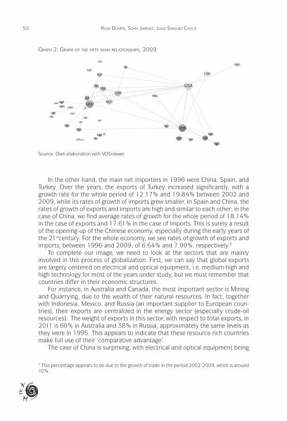
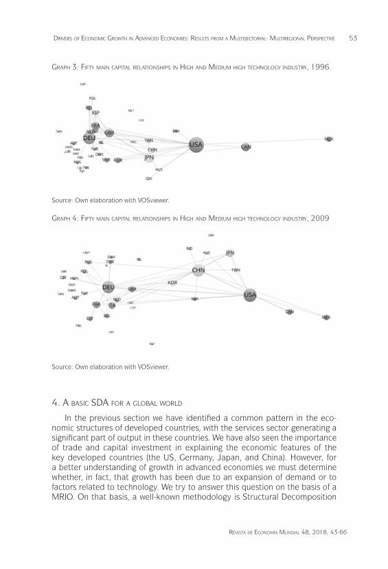
As we showed, high technology sector seems to be the favorite destination of external capital investment, so we choose it as a representative sector to study in depth the relationships established between countries (see graphs 3 and 4). First, we observe that, in 2009 there are more and newer links be-tween countries than in 1996; in other words, there is an opening of capital investment in high and medium-high technology industry. In 1996, we see six clusters, while in 2009 we observe only four. However, in 2009, there are more capital movements between European countries, as well as between Asiatic countries. In 1996, there were six key countries; the US, Japan, Canada, Ger-many, the UK, and France, the three last from the same cluster. In 2009, we only have four key countries: the US, Germany, China, and Japan (followed by South Korea, France, the UK, and Italy). In the case of China, perhaps this reflects a strong process of structural change.

53



GrAPh 3: fifty mAin cAPitAl relAtionshiPs in hiGh AnD meDium hiGh technoloGy inDustry, 1996.


GrAPh 4: fifty mAin cAPitAl relAtionshiPs in hiGh AnD meDium hiGh technoloGy inDustry, 2009


4. A bAsic sDA for A GlobAl worlD

In the previous section we have identified a common pattern in the eco-nomic structures of developed countries, with the services sector generating a significant part of output in these countries. We have also seen the importance of trade and capital investment in explaining the economic features of the key developed countries (the US, Germany, Japan, and China). However, for a better understanding of growth in advanced economies we must determine whether, in fact, that growth has been due to an expansion of demand or to factors related to technology. We try to answer this question on the basis of a MRIO. On that basis, a well-known methodology is Structural Decomposition



-30

-20

-10

0

10

20

30

40

19961997199819992000200120022003200420052006200720082009




-30

-20

-10

0

10

20

30

40

19961997199819992000200120022003200420052006200720082009



Analysis (SDA forward) that let us clearly identify different sources of growth year by year and both for the aggregate economy and for each region, some-thing that we cannot obtain through the use of other techniques.

4.1. methoDoloGy

SDA aims to separate a time trend of an aggregated variable into a group of driving forces that can act as accelerators or retardants (Dietzen-bacher and Los, 1998; Hoekstra and van den Bergh, 2002; Lenzen et al.., 2001). A basic idea that underlies the analysis is the independence of the explanatory factors involved. As we are working within an input-output frame, the starting point is the basic equation of the input-output model:

x= Ax+y; x=(I-A)-1y (1)

where x reflects the output’s vector, A is the matrix of technical coefficients, and y is the vector of final demand. From (1), if c is the vector of value-added coefficients respect to output, we can obtain the vector v of value added,

v=c’(I-A)-1y=c’Ly (2)

As we can observe in (2), if we try to do an SDA analysis of value added, we find dependency problems between c and (I-A)-1, which we are going to call L, and this can imply biased results. In order to avoid this full dependence problem, we base our analysis on the SDA proposal by Dietzenbacher & Los (2000), who construct an ‘intermediate’ Leontief’s inverse based on a matrix of technological coefficients, Ã, that has in each column the same distribution of coefficients as the matrix of coefficients A. Ã can be obtained by multiplying the elements in A by scalars representing row sums, as we show

with sr’ =e’Ar (i, j =0,1) (3)

In that way, we can decompose value added increments in three effects

(4)

Note that, following ‘the principle of nested or hierarchical decomposi-tions’, since we use three explanatory factors, we can obtain three more de-compositions but equivalent to expression (4). They are

(5)

12

v=c’(I-A)-1y=c’Ly (2)

As we can observe in (2), if we try to do an SDA analysis of value added, we find dependency problems between c and (I-A)-1, which we are going to call L, and this can imply biased results. In order to avoid this full dependence problem, we base our analysis on the SDA proposal by Dietzenbacher & Los (2000), who construct an ‘intermediate’ Leontief’s inverse based on a matrix of technological coefficients,𝐀𝐀, that has in each column the same distribution of coefficients as the matrix of coefficients A. 𝑨𝑨 can be obtained by multiplying the elements in A by scalars representing row sums, as we show

𝐀𝐀𝐢𝐢 = 𝐀𝐀𝐢𝐢𝐬𝐬𝐢𝐢&𝟏𝟏𝐬𝐬𝐣𝐣 with sr’ =e’Ar (i, j =0,1) (3)


Δv = c,L,-c0L, y, + c0 L,-L0 y, + c0L0(Δy) (4)

Note that, following ‘the principle of nested or hierarchical decompositions’, since we use three explanatory factors, we can obtain three more decompositions but equivalent to expression (4). They are

Δv = c,L,-c0L, y0 + c0 L,-L0 y0 + c,L, Δy = c,L0-c0L0 y0 + c, L,-L0 y0 +c,L, Δy = c,L0-c0L0 y, + c, L,-L0 y, + c0L0(Δy) (5)

As a commitment solution, the average of all the decompositions is used in the analysis

Δv = FE + SE + DE

With this decomposition, value added changes can be explained on the basis of three main drivers. The first element can be called the fabrication effect (FE) and indicates the substitution between total intermediate inputs and ‘value added terms’. It represents a sort of index of technological change in so far as it captures the more or less intensive use of labour, rather than technology, which is reflected in technical coefficients. The second element is called the substitution effect (SE) and reflects the effect of changes in the mix of intermediate inputs. In this regard, it is a proxy of structural change, since it captures how intermediate consumption is distributed between sectors and countries. Finally, the demand effect (DE) captures the contribution of final demand changes (all other things being constant) to income growth.

As we are working with multiregional input-output tables, we use a square matrix of final demand, created through the formation of diagonal matrices by parts. This is a block matrix (Bij) where each block Bij is a diagonal matrix of final demand of country i produced in j. In that way, we can take into account imports of final products of each country as part of the final demand of these countries. The analysis is carried out on a year by year basis.

12

v=c’(I-A)-1y=c’Ly (2)

As we can observe in (2), if we try to do an SDA analysis of value added, we find dependency problems between c and (I-A)-1, which we are going to call L, and this can imply biased results. In order to avoid this full dependence problem, we base our analysis on the SDA proposal by Dietzenbacher & Los (2000), who construct an ‘intermediate’ Leontief’s inverse based on a matrix of technological coefficients,𝐀𝐀, that has in each column the same distribution of coefficients as the matrix of coefficients A. 𝑨𝑨 can be obtained by multiplying the elements in A by scalars representing row sums, as we show

𝐀𝐀𝐢𝐢 = 𝐀𝐀𝐢𝐢𝐬𝐬𝐢𝐢&𝟏𝟏𝐬𝐬𝐣𝐣 with sr’ =e’Ar (i, j =0,1) (3)


Δv = c,L,-c0L, y, + c0 L,-L0 y, + c0L0(Δy) (4)

Note that, following ‘the principle of nested or hierarchical decompositions’, since we use three explanatory factors, we can obtain three more decompositions but equivalent to expression (4). They are

Δv = c,L,-c0L, y0 + c0 L,-L0 y0 + c,L, Δy = c,L0-c0L0 y0 + c, L,-L0 y0 +c,L, Δy = c,L0-c0L0 y, + c, L,-L0 y, + c0L0(Δy) (5)


Δv = FE + SE + DE

With this decomposition, value added changes can be explained on the basis of three main drivers. The first element can be called the fabrication effect (FE) and indicates the substitution between total intermediate inputs and ‘value added terms’. It represents a sort of index of technological change in so far as it captures the more or less intensive use of labour, rather than technology, which is reflected in technical coefficients. The second element is called the substitution effect (SE) and reflects the effect of changes in the mix of intermediate inputs. In this regard, it is a proxy of structural change, since it captures how intermediate consumption is distributed between sectors and countries. Finally, the demand effect (DE) captures the contribution of final demand changes (all other things being constant) to income growth.

As we are working with multiregional input-output tables, we use a square matrix of final demand, created through the formation of diagonal matrices by parts. This is a block matrix (Bij) where each block Bij is a diagonal matrix of final demand of country i produced in j. In that way, we can take into account imports of final products of each country as part of the final demand of these countries. The analysis is carried out on a year by year basis.

55




Δv=FE+SE+DE

With this decomposition, value added changes can be explained on the basis of three main drivers. The first element can be called the fabrication effect (FE) and indicates the substitution between total intermediate inputs and ‘value added terms’. It represents a sort of index of technological change in so far as it captures the more or less intensive use of labour, rather than technology, which is reflected in technical coefficients. The second element is called the substitution effect (SE) and reflects the effect of changes in the mix of intermediate inputs. In this regard, it is a proxy of structural change, since it captures how intermediate consumption is distributed between sec-tors and countries. Finally, the demand effect (DE) captures the contribution of final demand changes (all other things being constant) to income growth.

As we are working with multiregional input-output tables, we use a square matrix of final demand, created through the formation of diagonal matrices by parts. This is a block matrix (Bij) where each block Bij is a diago-nal matrix of final demand of country i produced in j. In that way, we can take into account imports of final products of each country as part of the final demand of these countries. The analysis is carried out on a year by year basis.

4.2. mAin results

Table 5 and graph 5 show the main results of our analysis. In graph 5, we can observe the evolution of the three effects from 1996 to 2009, whereas in Table 5 we show the average value of each effect as a percentage of value added of 2009. The main conclusion is obvious; the more important factor in explaining increments of value added, in almost all periods, is the change of final demand. This effect is especially significant for the period 2002-2009 (see the average values in Graph 5), achieving a maximum of 12% (with respect to the value added of the previous year) in 2004. So, the evolution followed by the demand effect is also interesting. The demand effect experienced a moderate increase between 1998 and 2000, when we observe a decrease, which may be due to the TIC crisis that occurred in those years. However, since then there has been a constant decline, al-though achieving values (around 4%) in 2004 that are higher than those observed at the beginning of the period analysed. This strong decline could be a signal of the crisis that would begin in 2007.


GrAPh 5: fAbricAtion, substitution, AnD DemAnD effects inGlobAl terms, 1996-2009.


We also notice that both fabrication and substitution effects are near zero throughout the period. Nevertheless, we must take into account that, in relative terms, these values are not so weak. In Table 1, we see that the fabrication effect is over 0.5% in a majority of the countries. However, a positive value of the fabrica-tion effect appears to be followed, immediately, by negative values of the substitu-tion effect. This is more evident from 2001 until 2006. However, as we have said, in almost all countries studied in the early years of the 21st century, we can observe a positive fabrication effect, which is an indicator of technological improvement.

In this way, focusing our attention on Table 5, we can get a more detailed analysis. For instance, the area with the highest values of the demand effect is Europe, probably due to their internal politics, obtaining an average value of 11.15% of 2009 value added. Asiatic countries come second, with values around 8% (a difference of 3 percentage points).

Here, we also must take into account the effect of external demand. For ex-ample, countries such as the US and Germany had an external demand effect of 0.89% and 2.61% respectively, but the domestic effect is higher. This situ-ation is repeated through most countries, with average values of the external and domestic demand effects of 3.82% and 6.41%, respectively, suggesting a direct relationship between demand and economic growth.

With respect to the substitution and fabrication effects, we do not observe such high values as might be expected after our global analysis. The case of Denmark is interesting, since its substitution effect was -46.47% and its fabri-cation effect was 28.39%, reflecting the importance of its positive fabrication effect (improvements in productivity) and the negative effect of a change in the mix of intermediate inputs (increments in the input cost per unit). Note that a positive fabrication effect means that there is an increase of value-added for fixed values of input costs and final demand.

13

4.2. MAIN RESULTS.

Table 5 and graph 5 show the main results of our analysis. In graph 5, we can observe the evolution of the three effects from 1996 to 2009, whereas in Table 5 we show the average value of each effect as a percentage of value added of 2009. The main conclusion is obvious; the more important factor in explaining increments of value added, in almost all periods, is the change of final demand. This effect is especially significant for the period 2002-2009 (see the average values in Graph 5), achieving a maximum of 12% (with respect to the value added of the previous year) in 2004. So, the evolution followed by the demand effect is also interesting. The demand effect experienced a moderate increase between 1998 and 2000, when we observe a decrease, which may be due to the TIC crisis that occurred in those years. However, since then there has been a constant decline, although achieving values (around 4%) in 2004 that are higher than those observed at the beginning of the period analysed. This strong decline could be a signal of the crisis that would begin in 2007.

GRAPH 5: FABRICATION, SUBSTITUTION, AND DEMAND EFFECTS INGLOBAL TERMS, 1996-2009.


We also notice that both fabrication and substitution effects are near zero throughout the period. Nevertheless, we must take into account that, in relative terms, these values are not so weak. In Table 1, we see that the fabrication effect is over 0.5% in a majority of the countries. However, a positive value of the fabrication effect appears to be followed, immediately, by negative values of the substitution effect. This is more evident from 2001 until 2006. However, as we have said, in almost all countries studied in the early years of the 21st century, we can observe a positive fabrication effect, which is an indicator of technological improvement.

In this way, focusing our attention on Table 5, we can get a more detailed analysis. For instance, the area with the highest values of the demand effect is Europe, probably due to their internal politics, obtaining an average value of 11.15%

-2

0

2

4

6

8

10

12

14

1997 1998 1999 2000 2001 2002 2003 2004 2005 2006 2007 2008 2009

FABRICATION SUSBTITUTION DEMAND

57



tAble 1: AverAGe DemAnD, fAbricAtion AnD substitution effect As PercentAGe of 2009 vAlue ADDeD.

DemandExternal demand

Domestic demand

Substitution Fabrication

Australia 11.05 1.55 9.50 0.36 0.34Austria 7.18 3.52 3.66 0.14 -0.34Belgium 7.21 3.64 3.57 -0.47 -0.10Bulgaria 15.80 8.29 7.51 9.76 -1.63

Brazil 9.36 0.92 8.45 -0.14 0.09Canada 9.74 2.54 7.21 0.86 0.19China 9.70 4.91 4.79 0.72 -0.24

Cyprus 10.19 1.87 8.32 0.64 -0.35Czech Republic 11.86 7.22 4.64 0.99 0.29

Germany 5.90 2.61 3.29 -0.71 0.19Denmark 9.26 2.66 6.60 -46.47 28.39

Spain 9.93 2.08 7.85 0.87 -0.14Estonia 17.36 8.65 8.71 1.76 0.68Finland 10.69 2.92 7.77 0.64 -0.73France 7.61 1.96 5.65 0.02 0.07

UK 7.61 2.68 4.93 -0.65 -0.07Greece 10.36 1.74 8.62 0.25 0.20

Hungary 11.70 6.82 4.88 -0.02 0.31Indonesia 12.46 0.99 11.48 -1.40 0.15

India 6.96 2.69 4.27 -0.15 -0.03Ireland 12.89 8.06 4.83 3.24 -0.35

Italy 10.79 2.10 8.69 0.39 -0.21Japan -2.15 0.71 -2.86 -0.94 -0.27Korea 7.66 2.51 5.15 0.07 -0.25

Lithuania 13.96 7.43 6.52 0.66 1.33Luxemburg 8.72 8.43 0.29 4.61 -2.62

Latvia 14.76 6.38 8.39 -1.84 -0.25Mexico 7.80 1.65 6.15 -1.16 0.21Malta 27.35 4.24 23.12 -2.99 -0.73

Netherlands 7.76 3.58 4.17 -0.73 0.07Poland 9.63 4.39 5.24 -0.18 0.55

Portugal 9.40 1.88 7.52 -0.10 0.04Romania 10.32 4.70 5.62 -0.30 -1.64Russia 11.81 3.82 7.99 3.97 0.71

Slovakia 11.62 8.00 3.62 0.85 0.67Slovenia 10.34 4.93 5.41 -0.77 0.92Sweden 10.93 3.51 7.42 -0.14 0.72Turkey 12.25 2.86 9.39 1.27 -0.28Taiwan 5.89 2.24 3.65 -2.46 0.47USA 5.29 0.89 4.41 -0.59 0.04

Average value 10.22 3.82 6.41 -0.75 0.66European Union 11.15 4.60 6.55 -1.13 0.94North America 7.52 1.72 5.81 0.13 0.12Asia and Pacific 8.40 2.47 5.93 0.16 0.07



Following this argument, we can analyze which sectors make greater con-tributions to each effect, and to each country. From the results obtained (avail-able on request), we can highlight the high-technology industries, and Services. We can say about demand effect that, in average terms, the services-related sectors are where we find the higher percentages. Moreover, the evolution of services is quite clear throughout the period, whereas percentages for industri-al sectors are more moderate. The main exception is China, where some indus-trial sectors, such as Basic Metals or Other non-metallic minerals, represents around 6% of the total demand effect. However, we must note that they are sectors of low or medium-low technology. The agriculture sector, although it achieves some importance in certain countries, such as Bulgaria, Rumania, and even China, is not, in general, a significant factor. If we focus on the fabrication effect, we can say that the construction sector, at the beginning of the period, is where the effect of substitution of intermediate consumption for value add-ed is highest, whereas at the end we find that the strongest fabrication effect is found in sectors such as Chemicals, and Rubber and Plastic products. Finally, with respect to the substitution effect, in 1997 we can find the energy sector as a key in the change of the mix of intermediate consumption, together with some parts of the services sector. However, whereas the energy sector weak-ens throughout the period, the services sector increases its contribution to the substitution effect (for example, Real Estate Activities). Some high-technology sectors, such as equipment, have increased their importance in the contribu-tion to the substitution sector, achieving high values at the end of the period.

5. conclusions

The objective of this paper has been to provide an overview of the factors that influence growth in developed countries.

We have seen that the US and China have been the major producers be-tween 1996 and 2009. However, in per capita terms, Luxemburg appears in first position, which could be explained by its fiscal characteristics; for exam-ple, financial intermediation is the main sector in Luxemburg’s economy. In spite of such anomalies, we do find a common pattern in most countries, where services are central to developed economies and industry is stable.

External specialization is also important and developed countries tend to export products related to high and medium-high technology sectors, although – not surprisingly – we see that countries rich in resources center their exports on mining and quarrying or the energy sector, using their comparative advantage.

One important variable to explain growth is capital investment, although the direction of such investment is as important as the amount. We find certain variations. The US directs almost 40% of its total to equipment, while other countries devote less than half of that proportion. We also note that capital in-vestment, particularly by the US and Canada, has been in a decline since 2005.

So, we can observe that in fact sectoral structure, or focus, matters as some literature claimed; Luque et al. (2015) and/or Fernández et al. (2008) among

59



others. This is especially evident from capital investment perspective, marking one of the main differences between countries.

After the descriptive analysis, we have run a basic SDA that let us to obtain three effects; demand, fabrication, and substitution effects. Our results reflect that global economic growth has been primarily due to changes in demand, especially in the early years of the 21stcentury. These results are in line with those obtained by Lobejón et al. (2007) for the Italian economy or Chóliz-Sánchez (2006) for the Spanish one. We find also, between 2001 and 2006 positive values of fabrication effect, which we take to be a proxy for technologi-cal change. Although values are not as high as those observed for the demand effect, we see values between 0.5% and 1% in most countries. These values can be relatively important, as they indicate a period of six years with continu-ous increments of productivity and of technological change.

In general, thinking about the results obtained, we can conclude that there were some signs of deceleration in developed economies before 2007, when the current crisis began. These signals are especially clear from 2004 to 2009. For example, the role of industry in the majority of the economies is decreasing each year; capital investment is located in the construction sector, rather than in equip-ment, where technology is more important; and in capital investment we see a de-celeration in important economies such as the US or some European economies (Germany or Finland, for instance). Moreover, the demand effect has decelerated since 2004, continuing to decrease until 2009, and there has been a continuous decline in the fabrication effect since 2006, reaching negative values in 2009.

This is a preliminary study, and we must carry out a more detailed analysis in the future, so that our subsequent objective is to examine how the factors studied in this paper determine different paths of growth and make an econo-my stronger, or weaker, especially when faced with difficult situations, such as the current, ongoing, economic crisis.

6. biblioGrAPhy

Arguelles. M & Benavides. C (2008): “Knowledge and Economic Growth. An Strat-egy for Developing Countries”, Revista de Economía Mundial, 18, 65-77.

Barro, J. (1989): “Economic Growth in a Cross Section of Countries”, The Quarterly Journal of Economics, Vol. 106, No. 2., pp. 407-443.

Benhabib. J & Spiegel. M. M. (1994): “The Role of Human Capital in Eco-nomic Development. Evidence from Aggregate Cross-country Data”, Jour-nal of Monetary Economics, 34, 143-173.

Bulman. D, Eden. M & Nguyen. H (2017): “Transitioning from Low Income Growth to High-income Growth: Is There a Middle-income Trap?”, Journal of the Asia Pacific Economy, 22(1), 5-28

Crespo Cuaresma. J, Doppelhofer. G & Feldkircher. M (2014): “The Determinants of Economic Growth in European Regions”, Regional Studies, 48(1), 44-67

Diaz, A & Franjo, L (2014): “Capital Goods, Measured TFP and Growth: The


Case of Spain”, Working Papers 201401, Center for Fiscal Policy, Swiss Federal Institute of Technology Lausanne, revised Oct 2014.

Dietzenbacher, E & Los, B (2000): “Structural Decomposition Analyses with Dependent Determinants”, Economic Systems Research, 12:4, 497-514.

Fernández Sánchez, R & Palazuelos Manso (2010): “Labour Productivity and Sectoral Structures in European Economies”, Revista de Economía Mundi-al, 24, 213-243.

Hanushek, E. A. (2013): “Economic Growth in Developing Countries: The Role of Human Capital”, Economics of Education Review Volume 37, December 2013, Pages 204–212.

Hoekstra, R. and J.C.J.M van den Bergh, (2002): “Structural Decomposition Analysis of Physical Flows in the Economy”, Environmental and Resource Economics, 23, pp. 357-378.

Giménez. G, López-Pueyo. C & Sanaú. J (2015): “Human Capital Measurement in OECD Countries and its Relation to GDP Growth and Innovation”, Revista de Economía Mundial, 39, 77-108.

Lenzen, M. (2001): “A Generalized Input-Output Multiplier Calculus for Austra-lia”, Economic Systems Research, Vol 13, No 1, 65-91.

Lobejón Herrero. L. F. (2007): “Demand, Economic Growth and Monetary In-tegration: The Italian Case”, Revista de Economía Mundial, 17, 175-194.

Luque. V & Palazuelos. E (2015): “An Interpretation of Weak Growth of the Ger-man Economy in the Period 1995-2007”, Revista de Economía Mundial, 41, 159-180.

Murray, J and Lenzen, M (ed) (2013): The Sustainability Practitioner’s Guide to Multi-Regional Input-output Analysis. Common Ground.

Nelson, R. R. (1973): “Recent Exercises in Growth Accounting: New Under-standing or Dead End?”, The American Economic Review, 63(3), 462-468.

OECD (2016): Structural Analysis (STAN) Databases, www.oecd.orgRodríguez Ortiz. F (2010): “Global Economic Crisis and New Economic Para-

digms”, Revista de Economía Mundial, 177-201. Saviotti, P & Frenken, K (2008): “Export Variety and the Economic Performance

of Countries”, Journal of Evolutionary Economics, vol. 18(2), 201-218. Schumpeter, J.A. (1939): Business cycles, A Theoretical, Historical and Statis-

tical Analysis of the Capitalist Process. McGraw-Hill Book Company. Solow, R.M. (1956): “A Contribution to the Theory of Economic Growth”, The

Quarterly Journal of Economics 70 (1): 65-94.Szirmai, A (2013): “Industrialization as an Engine of Growth in Developing

Countries, 1950–2005”, Structural Change and Economic Dynamics, 23 (4), 406–420.

Timmer, M.P. (ed) (2012): “The World Input-Output Database (WIOD): Con-tents, Sources and Methods”, WIOD Working Paper Number 10.

Timmer, M. P., Dietzenbacher, E., Los, B., Stehrer, R. and de Vries, G. J. (2015): “An Illustrated User Guide to the World Input–Output Database: the Case of Global Automotive Production”, Review of International Economics., 23: 575–605.

61



AP

Pen

Dix

.

tAb

le 1

: co

un

trie

s in

wio

D D

AtA

bA

se.

Sour

ce: T

imm

er (e

d) (2

012

).

tAb

le 2

: vA

lue

AD

DeD

by

co

un

try

An

D s

ecto

riA

l sP

eciA

lizA

tio

n 1

99

6-2

00

9.

Valu

e ad

ded

% v

a/ou

tput

19

96

20

09

19

96

Per

capi

ta2

00

9Pe

r ca

pita

%%

Indu

stry

Serv

ices

Ave

rage

an

nual

rat

e1

99

62

00

91

99

62

00

91

99

62

00

9

Aus

tral

ia1

36

62

719

89

511

21,4

03

43

,18

81

4.5

88

.51

67

.82

67

.40

7.9

44

7.1

34

8.4

0

Aus

tria

218

57

43

58

95

52

6,3

35

40

,907

19

.64

18

.54

66

.61

69

.81

3.8

95

3.8

24

7.0

9

Bel

gium

25

88

45

44

08

26

24

,31

93

8,7

48

20

.28

14

.54

70.0

87

7.0

64

.18

45

.10

41.4

2

Bul

gari

a11

29

53

88

26

1,5

27

5,3

06

21.9

61

7.5

75

2.2

961

.83

9.9

641

.70

36

.92

Bra

zil

68

57

30

13

99

62

94

,49

87

,15

91

8.6

21

5.2

06

6.7

06

7.8

15

.64

53

.03

49

.03

Can

ada

55

55

83

14

35

75

01

9,1

77

36

,69

31

8.3

61

6.7

46

6.8

26

7.0

97

.58

52

.69

52

.15

Chi

na7

98

53

04

93

59

0770

33

,72

63

4.8

03

2.8

43

2.8

64

3.1

31

5.0

43

7.8

63

2.2

2


Cyp

rus

86

49

22

09

69

,84

21

9,2

57

11.8

06

.84

72

.46

80

.35

7.4

861

.15

56

.60

Cze

ch R

epub

lic51

714

18

54

78

5,4

25

16

,34

82

4.2

62

5.8

45

6.6

95

9.6

810

.32

37

.24

35

.73

Ger

man

y2

315

011

30

98

84

82

6,9

513

6,5

112

2.6

42

2.4

16

6.5

86

9.4

92

.27

53

.15

49

.53

Den

mar

k1

613

88

28

071

53

0,1

04

48

,29

61

7.1

211

.45

71.4

57

6.3

04

.35

52

.58

47

.71

Spai

n5

63

62

21

413

44

81

4,5

102

9,3

38

19

,19

13

.23

64

.86

72

.12

7.3

34

8.5

24

6.6

9

Esto

nia

351

51

79

46

2,9

47

12

,52

62

0.9

81

4.3

261

.24

70.9

61

3.3

64

2.2

54

4.8

9

Finl

and

118

39

621

75

76

21,7

75

38

,70

92

5.4

01

8.6

16

2.1

96

8.9

74

.79

47

.48

43

.41

Fran

ce1

42

23

63

25

207

99

23

,46

43

6,9

33

14

.24

10.1

27

2.1

07

9.9

04

.50

51.1

14

9.8

0

UK

107

871

52

32

318

51

8,9

17

31,9

98

20

.94

11.6

96

7.4

77

7.0

56

.08

48

.99

50

.17

Gre

ece

121

25

23

04

08

011

,68

62

6,3

37

11.9

910

.31

69

.64

79

.07

7.3

35

5.9

95

8.6

5

Hun

gary

39

513

12

370

93

,861

10,9

02

21.2

72

5.3

26

2,6

36

2.0

79

.18

41.7

341

.79

Indo

nesi

a2

59

33

05

37

43

21

,410

2,2

59

29

.48

22

.65

40

.28

38

.16

5.7

751

.24

50

.83

Indi

a3

78

49

51

30

86

52

38

21

,04

31

8.5

31

4.5

64

5.7

75

6.7

210

.01

48

.90

47

.50

Irel

and

65

072

22

74

43

18

,221

44

,341

30

.16

26

.77

54

.97

65

.58

10.1

04

4.0

541

.86

Italy

102

58

40

19

59

78

82

0,0

20

32

,18

32

2.2

31

6.5

86

6.4

27

3.1

75

.11

48

.13

46

.23

Japa

n5

39

55

50

44

38

621

36

,63

43

8,5

66

22

.59

18

.60

64

.57

71.7

3-1

.49

53

.40

49

.66

Kor

ea51

49

34

85

48

02

11,2

93

15

,27

92

7.2

131

.09

54

.04

58

.14

3.9

84

3.1

13

5.7

2

Lith

uani

a6

331

36

30

92

,10

510

,741

19

.13

16

.37

57

.54

69

.69

14

.38

47

.19

51.0

0

Luxe

mbu

rg1

901

05

09

20

45

,10

49

4,7

47

13

.69

6.4

67

7.2

48

6.6

07

.87

47

.10

34

.15

Latv

ia4

48

82

56

702

,04

711

,14

52

0.6

89

.94

60

.57

76

.06

14

.36

48

.28

45

.65

Mex

ico

32

77

35

100

807

63

,641

7,1

29

19

.88

17

.62

61.3

661

.13

9.0

35

4.3

35

7.4

3

Mal

ta3

34

27

32

28

,87

81

7,1

34

21.6

71

3.2

96

8.7

87

8.3

36

.22

48

.96

44

.38

Net

herl

ands

39

018

27

58

09

22

4,1

714

2,7

811

7.4

41

4.0

56

9.1

67

3.5

25

.24

47

.60

46

.65

Pola

nd1

29

58

54

79

072

3,5

74

10,0

97

21.1

11

8.0

75

6.8

36

4.4

910

.58

45

.47

44

.51

Port

ugal

102

44

421

32

83

10,2

19

19

,45

01

8.4

41

3.4

06

5.9

57

4.7

95

.80

46

.06

47

.45

63



Rom

ania

36

90

91

717

20

1,5

56

7,2

73

25

.57

23

.61

42

.38

54

.69

12

.55

43

.79

46

.34

Rus

sia

29

02

98

13

23

57

72

,53

37

,59

51

7.4

21

6.2

75

6.4

45

9.6

21

2.3

84

9.9

75

0.0

3

Slov

akia

18

87

78

22

03

3,5

44

14

,83

32

6.7

81

9.5

65

6.3

26

0.9

111

.98

37

.72

40

.87

Slov

enia

18

42

54

42

34

9,0

64

21,0

17

25

.69

19

.59

60

.47

66

.46

6.9

74

4.0

74

4.0

9

Swed

en2

24

93

24

06

73

02

7,3

30

37

,71

62

2.3

91

6.7

36

6.4

971

.02

4.6

64

7.9

04

6.5

5

Turk

ey2

27

43

56

22

45

83

,89

37

,55

42

9.2

91

8.4

45

0.0

06

3.1

78

.05

55

.58

48

.72

Taiw

an2

84

04

03

87

57

71

2,9

24

15

,44

92

6.5

12

2.9

96

2.2

071

.37

2.4

24

7.2

64

6.2

0

USA

77

30

078

14

04

29

23

29

,12

34

5,6

38

15

.50

12

.25

75

.77

79

.38

4.7

05

5.0

75

5.2

5

RoW

30

521

98

82

35

59

79

21

78

29

.43

45

.79

23

.76

42

.18

7.9

351

.06

49

.05

Sour

ce: O

wn

elab

orat

ion.

tAb

le 3

: exP

ort

s A

nD im

Po

rts

for e

Ac

h c

ou

ntr

y fo

r y

eAr

s 1

99

6, 2

00

2, A

nD 2

00

9.

1

99

62

00

9A

vera

ge r

ate

of

grow

th e

xpor

tsA

vera

ge r

ate

of

grow

th im

port

s

Diff

eren

ce

grow

th r

ates

ex

port

s-im

port

s

Ex

port

sIm

port

sN

et

expo

rts

Expo

rts

Impo

rts

Net

ex

port

s1

99

6-2

00

91

99

6-2

00

91

99

6-2

00

9

Aus

tral

ia4

64

03

64

73

86

16

65

01

671

26

107

58

65

95

40

7.6

66

.51

1.1

5

Aus

tria

48

46

94

59

49

25

20

110

42

29

50

92

15

331

6.5

45

.75

0.7

8B

elgi

um10

55

67

101

25

44

313

19

54

86

18

66

39

88

47

4.8

54

.82

0.0

4B

ulga

ria

43

414

67

3-3

32

13

75

51

619

2-2

43

79

.28

10.0

3-0

.75

Bra

zil

42

23

94

20

59

18

01

28

716

112

62

21

60

93

8.9

57

.87

1.0

8C

anad

a1

45

59

411

17

58

33

83

62

62

38

321

63

24

46

05

84

.63

5.2

1-0

.58

Chi

na7

80

26

101

706

-23

68

06

810

53

83

80

06

-15

69

53

18

.14

17

.61

0.5

2C

ypru

s9

65

218

5-1

22

02

818

46

42

-18

25

8.5

95

.97

2.6

2

Cze

ch R

epub

lic1

79

55

19

42

7-1

47

27

301

17

921

4-6

20

311

.39

11.4

2-0

.02

Ger

man

y3

39

516

27

95

75

59

941

74

06

09

59

03

29

15

02

80

6.1

85

.92

0.2

7D

enm

ark

321

1031

45

26

58

79

60

87

84

59

114

97

.23

7.2

8-0

.05

Spai

n6

42

77

814

22

-171

45

16

561

821

910

2-5

34

84

7.5

57

.91

-0.3

64 W

e fo

llow

the

sam

e or

der

as W

IOD

tab

les.


Esto

nia

14

89

18

81-3

92

671

45

807

907

12

.28

9.0

63

.22

Finl

and

313

912

38

29

75

62

618

23

54

705

711

85

.35

6.6

-1.2

5Fr

ance

19

241

31

83

38

09

03

33

23

35

83

52

40

6-2

90

49

4.0

75

.15

-1.0

8U

K2

05

614

18

38

33

217

82

38

42

53

33

031

15

39

42

4.9

34

.61

0.3

2G

reec

e5

613

16

700

-110

87

314

79

50

941

-19

46

21

4.1

88

.96

5.2

3H

unga

ry10

95

41

419

8-3

24

35

22

02

581

52

-59

50

12

.76

11.4

61

.31

Indo

nesi

a4

28

28

42

63

41

94

102

708

80

55

82

215

06

.96

5.0

21

.94

Indi

a2

54

45

33

361

-791

710

97

53

19

04

37

-80

68

511

.91

4.3

4-2

.44

Irel

and

25

703

30

44

4-4

741

12

58

24

121

73

44

09

01

311

.25

1.7

4Ita

ly1

46

69

41

48

64

7-1

95

32

45

32

53

08

58

2-6

32

57

4.0

35

.78

-1.7

4Ja

pan

28

24

06

23

015

85

22

48

43

38

84

37

25

95

612

89

3.3

63

.78

-0.4

2K

orea

97

74

811

09

89

-13

241

27

54

55

28

08

03

-53

48

8.3

7.4

0.8

9Li

thua

nia

211

92

72

8-6

09

117

22

110

54

66

81

4.0

611

.36

2.7

Luxe

mbu

rg1

641

611

88

54

531

641

90

551

24

90

66

11.0

61

2.5

3-1

.47

Latv

ia1

59

91

58

910

64

87

58

48

64

011

.37

10.5

40

.83

Mex

ico

57

93

26

63

95

-84

62

13

03

84

14

37

21-1

33

38

6.4

46

.12

0.3

2

Mal

ta1

35

41

76

7-4

13

34

613

32

31

37

7.4

94

.98

2.5

1

Net

herl

ands

12

95

90

121

03

38

55

72

718

04

25

39

56

17

84

85

.86

5.8

70

Pola

nd2

081

021

77

9-9

68

961

88

103

82

0-7

63

21

2.5

12

.76

-0.2

7Po

rtug

al1

39

52

231

04

-91

52

34

312

43

912

-96

00

7.1

75

.06

2.1

Rom

ania

58

23

88

08

-29

86

30

331

371

06

-67

75

13

.54

11.7

1.8

4

Rus

sia

76

35

42

901

44

73

412

57

36

07

20

66

18

52

94

9.8

7.2

52

.55

Slov

akia

74

47

819

2-7

45

33

94

23

69

92

-30

511

2.3

81

2.3

0.0

8Sl

oven

ia4

87

55

913

-10

39

14

007

15

29

8-1

29

28

.46

7.5

90

.87

Swed

en61

40

95

22

72

913

71

20

65

410

12

42

19

412

5.3

35

.22

0.1

2

Turk

ey1

49

72

28

681

-13

709

66

65

36

69

37

-28

41

2.1

76

.74

5.4

4

Taiw

an7

93

43

811

99

-18

56

18

072

31

42

90

53

781

96

.54

4.4

42

.09

USA

55

6101

49

25

45

63

55

69

69

24

410

114

97

-42

25

34

.37

5.6

9-1

.33

Tota

l3

061

491

28

45

80

421

56

87

706

48

416

85

60

36

20

88

05

6.6

47

-0.3

5

Sour

ce: O

wn

elab

orat

ion

65



tAb

le 4

: in

vest

men

t (in

us

mil

lio

ns

Do

llA

rs)

An

D P

erc

entA

Ge

of

inve

stm

ent

by s

ecto

rs,

wit

h r

esP

ect

to t

otA

l in

vest

men

t.

C

onst

ruct

ion

Equi

pmen

tSe

rvic

esTo

tal

econ

omy

Tota

l ec

onom

ySu

m o

f pe

rcen

tage

sSu

m o

f pe

rcen

tage

s

1

99

62

00

91

99

62

00

91

99

62

00

91

99

62

00

91

99

62

00

9

%

%%

%%

%

A

ustr

alia

76

.68

24

.69

4.0

81

.77

15

.68

24

.75

218

,02

04

98

72

49

6.4

451

.21

Aus

tria

54

.63

54

.49

7.5

12

.91

9.1

321

.53

521

96

76

28

881

.27

78

.92

Bel

gium

59

.92

59

.46

3.2

50

.67

21.6

72

5.2

84

80

24

913

45

84

.84

85

.41

Bul

gari

a5

9.4

66

7.6

91

2.2

87

.81

6.9

911

.86

17

20

12

68

77

8.7

38

7.3

6

Bra

zil

51.9

95

5.3

52

5.7

72

2.2

111

.23

13

131

36

82

48

40

58

8.9

99

0.5

6C

anad

a7

5.7

671

.78

55

.37

11.6

11

3.7

710

35

24

270

87

29

2.3

79

0.9

2C

hina

66

.83

65

.12

0.8

32

3.6

74

.76

8.4

12

86

82

62

281

48

09

2.4

29

7.1

8C

ypru

s8

4.4

57

6.5

90

.23

1.1

79

.13

13

.46

17

84

47

219

3.8

191

.22

Cze

ch R

epub

lic5

7.8

85

9.7

58

.78

14

.51

2.6

51

7.3

31

912

941

12

47

9.3

191

.58

Ger

man

y5

8.0

35

2.3

51

2.8

31

5.4

41

7.6

61

8.4

84

821

08

54

55

05

88

.52

86

.27

Den

mar

k5

9.9

95

6.8

32

.42

2.4

32

5.7

42

7.4

30

00

95

05

85

88

.15

86

.66

Spai

n6

8.8

86

73

.99

2.7

81

8.3

71

9.4

61

26

781

33

86

4191

.24

89

.24

Esto

nia

56

.19

67

.88

.28

0.7

61

6.0

32

2.8

511

68

37

95

80

.591

.41

Finl

and

617

6.3

411

.85

.46

17

.47

13

.121

45

34

34

66

90

.27

94

.9

Fran

ce5

6.4

65

5.4

77

.82

4.9

42

7.6

42

9.5

42

49

46

94

78

95

591

.92

89

.95

UK

55

.12

60

.66

.38

4.3

12

2.2

42

71

901

27

29

99

618

3.7

491

.91

Gre

ece

75

.73

64

.36

.07

4.3

31

2.8

22

0.1

92

36

74

52

82

99

4.6

28

8.8

2H

unga

ry5

3.0

45

4.8

10.9

68

.88

18

.21

19

.691

22

24

92

88

2.2

18

3.2

8In

done

sia

79

.89

0.3

71

4.5

83

.66

4.9

34

.68

72

83

61

67

891

99

.31

98

.71

Indi

a4

9.2

56

5.2

23

0.6

81

7.5

77

.54

8.6

48

69

0141

38

99

87

.47

91.4

3Ir

elan

d7

8.5

58

36

.52

5.8

9.9

19

.64

12

361

30

80

69

4.9

89

8.4

4Ita

ly5

3.1

25

2.7

11

6.6

21

3.2

41

9.4

721

.77

22

591

53

801

42

89

.21

87

.72


Japa

n6

0.0

15

5.5

52

0.4

81

7.2

61

5.3

21

9.1

51

310

59

210

44

20

09

5.8

191

.96

Kor

ea6

3.4

36

5.4

22

.13

17

.64

9.9

511

.78

19

48

69

22

76

05

95

.51

94

.82

Lith

uani

a7

4.7

36

8.9

83

.28

1.8

91

2.0

92

0.2

21

66

76

217

90

.191

.09

Luxe

mbu

rg7

6.2

47

7.5

81

.23

0.0

11

5.9

61

5.2

38

42

86

06

93

.43

92

.79

Latv

ia7

3.6

76

7.4

44

.24

0.5

111

.65

23

.17

88

05

38

88

9.5

691

.12

Mex

ico

69

.39

72

.57

10.5

35

.18

9.1

48

.96

33

42

18

33

69

89

.06

86

.65

Mal

ta41

.56

51.1

68

.77

0.2

11

9.1

62

7.7

47

87

113

26

9.4

97

9.1

1

Net

herl

ands

56

.64

47

.94

2.9

41

.18

26

.63

4.1

881

97

51

37

851

86

.18

83

.3

Pola

nd61

.58

56

.44

14

.76

6.3

71

2.9

32

2.7

22

87

50

861

48

89

.27

85

.53

Port

ugal

63

.87

63

.37

8.8

25

.84

19

.07

20

.88

26

791

44

20

891

.76

90

.09

Rom

ania

59

72

.02

32

.25

12

.86

.84

8.9

79

66

415

39

98

.09

93

.72

Rus

sia

74

,52

68

.72

10.6

31

4.9

7.6

61

5.4

571

02

02

212

37

92

.81

99

.07

Slov

akia

61.5

86

9.9

79

.06

6.0

71

4.3

41

4.4

63

54

17

49

38

4.9

89

0.4

4Sl

oven

ia6

2.5

76

9.5

51

2.0

71

.29

13

.54

18

.68

43

43

109

00

88

.18

89

.52

Swed

en5

0.6

26

0.3

27

.46

9.1

42

5.0

62

2.7

741

00

26

58

30

83

.14

92

.23

Turk

ey6

5.0

15

4.2

17

.611

.611

.65

20

.13

561

40

99

87

69

4.2

68

5.9

3

Taiw

an6

3.9

25

7.1

31

6.6

66

.22

16

.48

27

.39

621

77

64

04

99

7.0

69

0.7

4

USA

49

.01

40

.08

22

.66

18

18

.67

22

.63

14

80

66

72

29

06

63

90

.34

80

.71

TOTA

L5

55

61

71

521

23

5,8

37

,68

010

,91

3,3

56

93

94

Ave

rage

62

.76

2.5

11.3

7.6

14

.91

8.7

14

59

42

27

28

33

.98

9.2

38

8.8

Sour

ce: O

wn

elab

orat

ion.

Documents

D of e G in A e multireGionAl PersPective