Crop Disease and Agricultural Productivity

We

NBER WORKING PAPER SERIES

CROP DISEASE AND AGRICULTURAL PRODUCTIVITY

Christine L. CarrollColin A. Carter

Rachael E. GoodhueC.-Y. Cynthia Lin Lawell

Working Paper 23513http://www.nber.org/papers/w23513

NATIONAL BUREAU OF ECONOMIC RESEARCH1050 Massachusetts AveCambridge MA 02138

June 2017

We thank Krishna V. Subbarao, Julian Alston, Andre Boik, Colin Cameron, Erich Muehlegger, Kevin Novan, Peter Orazem, John Rust, Wolfram Schlenker, Paul Scott, Dan Sumner, Sofia Villas-Boas, Marca Weinberg, Jim Wilen, and Jinhua Zhao for invaluable discussions and comments. We also received helpful comments from seminar participants at the University of California at Davis and California State University at Chico, and from conference participants at the NBER Understanding Productivity Growth in Agriculture Research Conference, the Heartland Environmental and Resource Economics Workshop, the Association of Environmental and Resource Economists (AERE) Summer Conference, the American Agricultural Economics Association (AAEA) Annual Meeting, the Giannini Agricultural and Resource Economics Student Conference, and the Interdisciplinary Graduate and Professional Student (IGPS) Symposium. We received funding from USDA NIFA (grant # 2010-51181-21069). We also benefited from valuable discussions with Tom Bengard, Bengard Ranch; Kent Bradford, Seed Biotechnology Center UC-Davis; Leslie Crowl, Monterey County Agricultural Commissioner's Office; Rich DeMoura, UC-Davis Cooperative Extension; Gerard Denny, INCOTEC; Lindsey du Toit, Washington State University; Thomas Flewell, Flewell Consulting; Hank Hill, Seed Dynamics, Inc.; Steve Koike, Cooperative Extension Monterey County; Dale Krolikowski, Germains Seed Technology; Chester Kurowski, Monsanto; Donald W. McMoran, WSU Extension; Marc Meyer, Monsanto; Chris Miller, Rijk Zwaan; Augustin Ramos, APHIS; Scott Redlin, APHIS; Richard Smith, Cooperative Extension Monterey County; Laura Tourte, UC Cooperative Extension Santa Cruz County; Bill Waycott, Monsanto; and Mary Zischke, California Leafy Greens Research Program. Carter, Goodhue, and Lin Lawell are members of the Giannini Foundation of Agricultural Economics. All errors are our own. The views expressed herein are those of the authors and do not necessarily reflect the views of the National Bureau of Economic Research.

NBER working papers are circulated for discussion and comment purposes. They have not been peer-reviewed or been subject to the review by the NBER Board of Directors that accompanies official NBER publications.

© 2017 by Christine L. Carroll, Colin A. Carter, Rachael E. Goodhue, and C.-Y. Cynthia Lin Lawell. All rights reserved. Short sections of text, not to exceed two paragraphs, may be quoted without explicit permission provided that full credit, including © notice, is given to the source.

Crop Disease and Agricultural ProductivityChristine L. Carroll, Colin A. Carter, Rachael E. Goodhue, and C.-Y. Cynthia Lin LawellNBER Working Paper No. 23513June 2017JEL No. Q00,Q10,Q12

ABSTRACT

Crop diseases and how they are managed can have a large impact on agricultural productivity. This paper discusses the effects on agricultural productivity of Verticillium dahliae, a soil borne fungus that is introduced to the soil via infested spinach seeds and that causes subsequent lettuce crops to be afflicted with Verticillium wilt. We use a dynamic structural econometric model of Verticillium wilt management for lettuce crops in Monterey County, California to examine the effects of Verticillium wilt on crop-fumigation decisions and on grower welfare. We also discuss our research on the externalities that arise with renters, and between seed companies and growers due to Verticillium wilt, as these disease-related externalities have important implications for agricultural productivity.

Christine L. CarrollCollege of AgricultureCSU Chico940 West First StreetChico, CA [email protected]

Colin A. CarterUniversity of California at Davis Agricultural and Resource Economics One Shields AvenueDavis, CA [email protected]

Rachael E. GoodhueUniversity of California at Davis Agricultural and Resource Economics One Shields AvenueDavis, CA 95616 [email protected]

C.-Y. Cynthia Lin Lawell University of California at Davis Agricultural and Resource Economics One Shields AvenueDavis, CA [email protected]

1 Introduction

Crop diseases can have a large impact on agricultural productivity. Invasive plant pathogens,

including fungi, cause an estimated $21 billion in crop losses each year in the United States

(Rossman, 2009). Verticillium dahliae is a soil borne fungus that is introduced to the soil

via infested spinach seeds and that causes subsequent lettuce crops to be a�icted with

Verticillium wilt (V. wilt). Lettuce is an important crop in California, and the majority of

the lettuce production in the United States occurs in California. The value of California's

lettuce crop was $1.7 billion in 2013 (National Agricultural Statistics Service, 2015).

How crop diseases are managed can have a large impact on agricultural productivity

as well. V. wilt can be prevented or controlled by the grower by fumigating with methyl

bromide, planting broccoli (a low-return crop), or not planting spinach. These control options

entail incurring costs or foregoing pro�t in the current period for future bene�t. V. wilt can

also be prevented or controlled by the spinach seed company by testing and cleaning the

spinach seeds. However, seed companies are unwilling to test or clean spinach seeds, as they

are not a�ected by this disease.

This paper analyzes the e�ects of V. wilt on agricultural productivity. In particular,

we use a dynamic structural econometric model of V. wilt management for lettuce crops in

Monterey County, California to examine the e�ects of V. wilt on crop-fumigation decisions

and on grower welfare. We also discuss our research on the externalities that arise with

renters, and between seed companies and growers due to V. wilt, as these disease-related

externalities have important implications for agricultural productivity.

We use a dynamic model for several reasons. First, the control options (fumigation,

planting broccoli, and not planting spinach) require incurring costs or foregoing pro�t in the

current period for possible future bene�t, and are thus are best modeled with a dynamic

model.2 Second, because cropping and fumigation decisions are irreversible (as is the damage

2Some of these actions may also generate bene�ts in the current period for the current crop. For example,in addition to being an investment in protecting potential future lettuce crops from V. wilt, methyl bromide

1

from V. wilt), because the rewards from cropping and fumigation decisions are uncertain,

and because growers have leeway over the timing of cropping and fumigation decisions, there

is an option value to waiting which requires a dynamic model (Dixit and Pindyck, 1994).

Third, Verticillium dahliae takes time to build up in the soil, and once present, persists for

many years.

There are several advantages to using a dynamic structural model to model grower crop

and fumigation decisions. First, unlike reduced-form models, a structural approach explicitly

models the dynamics of crop and fumigation decisions by incorporating continuation values

that explicitly model how expectations about the future a�ect current decisions.

A second advantage of the structural model is that we are able to estimate the e�ect of

each state variable on the expected payo�s from di�erent crop and fumigation choices, and

are therefore able to estimate parameters that have direct economic interpretations. The

dynamic model accounts for the continuation value, which is the expected value of the value

function next period. With the structural model we are able to estimate parameters in the

payo�s from di�erent crop and fumigation choices, since we are able to structurally model

how the continuation values relate to the payo�s from the crop and fumigation choices.

A third advantage of our structural model is that we can use the parameter estimates

from our structural model to simulate the e�ects of crop disease on agricultural productivity.

In particular, we run counterfactual simulations to analyze the e�ects of V. wilt on crop-

fumigation decisions and on grower welfare.

The balance of this paper proceeds as follows. Section 2 provides background on the

California lettuce industry, V. wilt, and options to control the disease. Section 3 is a brief

review of the relevant literature. Section 4 describes our dynamic structural econometric

model. Section 5 describes our data. We present our results in Section 6 and our counter-

factual simulations in Section 7. Section 8 concludes.

can also be bene�cial to the current crop of strawberries. However, on net, these control options generallyrequire incurring net costs or foregoing pro�t in the current period.

2

2 Background

California, a major agricultural producer and global trader, sustains signi�cant economic

damage from invasive plant pathogens. Fungi damage a wide variety of California crops,

resulting in yield- and quality-related losses, reduced exportability, and increased fungicide

expenditures (Palm, 2001).

Measured by value, lettuce ranks in the top ten agricultural commodities produced

in California (National Agricultural Statistics Service, 2015). Much of California's lettuce

crop is grown in Monterey County, where lettuce production value is 27% of the county's

agricultural production value (Monterey County Agricultural Commissioner, 2015). Approx-

imately ten to �fteen thousand acres are planted to lettuce in Monterey County each season

(spring, summer, and fall). Spinach, broccoli, and strawberries are also important crops in

the region.

Verticillium dahliae is a soil borne fungus that causes lettuce to be a�icted with V.

wilt. No e�ective treatment exists once plants are infected by the fungus (Xiao and Subbarao,

1998; Fradin and Thomma, 2006). The fungus can survive in the soil for fourteen years as

microsclerotia, which are resting structures that are produced as the pathogen colonizes

a plant. This system allows the fungus to remain in the soil even without a host plant.

When a susceptible host is planted, microsclerotia attack through the roots, enter the water

conducting tissue, and interfere with the water uptake and transport through the plant. If

the density of microsclerotia in the soil passes a threshold, a disease known as V. wilt occurs.

V. wilt �rst killed a lettuce (Lactuca sativa L.) crop in California's Parajo Valley in

1995. Prior to 1995, lettuce was believed to be immune. Since then, the disease has spread

rapidly through the Salinas Valley, the prime lettuce production region of California. By

2010, more than 150 �elds were infected with V. wilt (Atallah, Hayes, and Subbarao, 2011),3

3As not all the �elds that were infected by 2010 were known at the time Atallah, Hayes, and Subbarao(2011) was published, the number of �elds a�ected by 2010 �elds was actually even higher, numbering over175 �elds (Krishna Subbarao, personal communication, 2013).

3

amounting to more than 4,000 acres (Krishna Subbarao, personal communication, 2013).4

Although growers have resisted reporting the extent of the disease since 2010, it is likely

that the number of a�ected acres has increased since then (Krishna Subbarao, personal

communication, 2013).

Verticillium dahliae is introduced to the soil in three possible ways. First, V. wilt can

be spread locally from �eld to �eld by workers or equipment. Local spread is a relatively

minor contributor, however, and growers have taken steps to mitigate this issue themselves,

for example by cleaning equipment before moving between �elds.

Second, V. wilt is introduced to the soil via infested lettuce seeds. However, studies of

commercial lettuce seed lots from around the world show that fewer than 18% tested positive

for Verticillium dahliae and, of those, the maximum incidence of infection was less than 5%

(Atallah, Hayes, and Subbarao, 2011). These relatively low levels do not cause V. wilt in

lettuce at an epidemic level. Models of the disease suggest that it would be necessary for

lettuce seed to have an incidence of infection of at least 5% and be planted back to back for

three to �ve seasons in order for the disease to appear, with at least �ve subsequent seasons

required for the high disease levels currently seen (Atallah, Hayes, and Subbarao, 2011).

Third, V. wilt is introduced to the soil via infested spinach seeds. Spinach seeds have

been shown to be the main source of the disease (du Toit, Derie, and Hernandez-Perez, 2005;

Short, D.P.G. et al., 2015); 89% of spinach seed samples are infected, with an incidence of

infected seeds per sample of mean 18.51% and range 0.3% to 84.8% (du Toit, Derie, and

Hernandez-Perez, 2005). The precise impact of planting infected spinach seeds on V. wilt

of lettuce was recently assessed and proven to be the cause of the disease on lettuce (Short,

D.P.G. et al., 2015). The pathogen isolated from infected lettuce plants is genetically identical

to the pathogen carried on spinach seeds (Atallah et al., 2010).

Infected spinach seeds carry an average of 200 to 300 microsclerotia per seed (Maruthacha-

4Krishna Subbarao is a Professor of Plant Pathology and Cooperative Extension Specialist at the Uni-versity of California at Davis. He has studied V. wilt for many years.

4

lam et al., 2013). As spinach crops are seeded at up to nine million seeds per hectare for

baby leaf spinach, even a small proportion of infected seeds can introduce many microscle-

rotia (du Toit and Hernandez-Perez, 2005).

One method for controlling V. wilt is to fumigate with methyl bromide. As methyl

bromide is an ozone depleting substance, the Montreal Protocol has eliminated methyl bro-

mide use for fumigation of vegetable crops such as lettuce; however, certain crops such as

strawberries have received critical-use exemptions through 20165 (California Department of

Pesticide Regulation, 2010; United States Environmental Protection Agency, 2012b), and

the residual e�ects from strawberry fumigation provide protection for one or two seasons

of lettuce before microsclerotia densities rise (Atallah, Hayes, and Subbarao, 2011). The

long-term availability of this solution is limited and uncertain.

A second method for controlling V. wilt is to plant broccoli. Broccoli is not susceptible

to V. wilt and it also reduces the levels of microsclerotia in the soil (Subbarao and Hubbard,

1996; Subbarao, Hubbard, and Koike, 1999; Shetty et al., 2000). Some growers have experi-

mented with this solution, but relatively low returns from broccoli in the region prevent this

option from becoming a widespread solution. Planting all infected acreage to broccoli may

also �ood the market, driving down broccoli prices.

A third method for controlling V. wilt is to not plant spinach, since spinach seeds are

the vector of pathogen introduction (du Toit, Derie, and Hernandez-Perez, 2005). Growers

who use this third control method of not planting spinach must forgo any relative pro�ts

they may have received if they planted spinach instead of another crop.

In addition to the control measures that the grower can take, V. wilt can also be pre-

vented or controlled by a spinach seed company through testing and cleaning the spinach

5Critical-use exemption requests through 2014 specify that up to one third of the California strawberrycrop will be fumigated with methyl bromide, but actual use was much lower. The remainder of the crop istreated with alternatives such as chloropicrin or 1,3-Dichloropropene (1,3-D) (United States EnvironmentalProtection Agency, 2012a). However, these alternatives (unless combined with methyl bromide) tend to beless e�ective for V. wilt (Atallah, Hayes, and Subbarao, 2011). Field trials of other chemical fumigants eitherhave not been widely used due to township caps or are not yet registered and approved.

5

seeds. Testing or cleaning seeds is an important option for preventing Verticillium dahliae

from being introduced into a �eld, but can be uncertain and potentially costly. Although

Verticillium dahliae cannot be completely eliminated by seed cleaning, incidence levels in

spinach seed can be signi�cantly reduced (du Toit and Hernandez-Perez, 2005). Very recent

developments in testing procedures suggest that testing spinach seed for Verticillium dahliae

might soon be feasible on a commercial basis. Moreover, a very recent innovation speeds

up testing spinach seeds. Previously, testing for Verticillium dahliae in spinach seeds took

approximately two weeks and could not accurately distinguish between pathogenic and non-

pathogenic species (Duressa et al., 2012). This new method takes only one day to complete,

is highly sensitive (as it is able to detect one infected seed out of 100), and can distinguish

among species (Duressa et al., 2012).

V. wilt can also be controlled by restricting the imports of spinach seeds infested with

Verticillium dahliae, but doing so would have trade implications. Currently, the United

States has no phytosanitary restrictions on spinach seed imports, but Mexico prohibits the

importation of seeds if more than 10% are infected (IPC, 2003).

V. wilt can therefore be prevented or controlled by the grower by fumigating with

methyl bromide, planting broccoli, or not planting spinach. These control options require

long-term investment for future gain. V. wilt can also be prevented or controlled by the

spinach seed company by testing and cleaning the spinach seeds. However, seed companies

are unwilling to test or clean spinach seeds, as they are not a�ected by this disease.

3 Literature Review

The �rst strand of literature to which our paper relates is on the economics of pest man-

agement (Hueth and Regev, 1974; Carlson and Main, 1976; Wu, 2001; Noailly, 2008; McKee

et al., 2009), which focuses on pests for which treatment is available after crops are a�ected.

In contrast, V. wilt cannot be treated once crops are a�ected. Existing work on crop disease,

6

such as Johansson et al. (2006) and Gomez, Nunez, and Onal (2009) on soybean rust, and

Atallah et al. (2015) on grapevine leafroll disease, focuses on spatial issues regarding the

spread of the disease. In contrast, V. wilt has only a limited geographic impact, and thus

dynamic considerations are more important than spatial ones for V. wilt.

A second strand of literature to which our paper relates is on dynamic models in

agricultural management. As Verticillium dahliae persists in the soil for many years, a

static model such as that proposed by Mo�tt, Hall, and Osteen (1984) will not properly

account for the future bene�ts of reducing microsclerotia in the soil. The dynamics of V.

wilt more closely �t the seed bank management model by Wu (2001).

Dynamic models have been used in agricultural management to analyze many prob-

lems. Weisensel and van Kooten (1990) use a dynamic model of growers' choices to plant

wheat, or to use tillage fallow versus chemicals to store moisture. In a related paper, van

Kooten, Weisensel, and Chinthammit (1990) use a dynamic model that explicitly includes

soil quality in the grower's utility function and the trade-o� between soil quality (which may

decline due to erosion) and net returns.

Our paper builds on the literature on dynamic structural econometric modeling. Rust's

(1987; 1988) seminal papers develop a dynamic structural econometric model using nested

�xed point maximum likelihood estimation. This model has been adapted for many ap-

plications, including bus engine replacement (Rust, 1987), nuclear power plant shutdown

(Rothwell and Rust, 1997), water management (Timmins, 2002), agriculture (De Pinto and

Nelson, 2009; Scott, 2013), air conditioner purchases (Rapson, 2014), wind turbine shut-

downs and upgrades (Lin Lawell, 2017), and copper mining decisions (Aguirregabiria and

Luengo, 2016). Carroll et al. (2017a) develop and estimate a dynamic structural model to

analyze short- versus long-term decision-making for disease control. Carroll et al. (2017b)

develop and estimate a dynamic structural model to analyze the supply chain externality

between growers and spinach seed companies in controlling V. wilt.

7

4 Dynamic Structural Econometric Model

To analyze the e�ects of V. wilt on, we develop and estimate a single-agent dynamic structural

econometric model using the econometric methods developed by Rust (1987). Each month

t, each grower i chooses an action dit ∈ D. The possible actions for each grower for each

month include one of �ve crops (resistant, susceptible (other than lettuce), lettuce, spinach,

and broccoli), combined with the choice to fumigate with methyl bromide. To focus on the

crops most relevant to this problem, we group the crops resistant to V. wilt together and the

crops (other than lettuce) susceptible to V. wilt together. Lettuce, spinach, and broccoli are

included separately as these crops are most relevant to V. wilt. Susceptible crops include

strawberries, artichoke, and cabbage. Resistant crops include cauli�ower and celery.

Although the raw data are observations on the day and time any fumigant is applied

on a �eld, we aggregate to monthly observations. Growers are generally only making one

crop-fumigation decision each season. The length of the season varies among crops, and can

be as short as one month for spinach and more than a year for strawberries. For this reason,

we choose a month as the time period for each crop-fumigation decision. To cover the case

of multi-month seasons, we include a dummy variable for whether the grower continues with

the same crop chosen in the previous month. Moreover, because not all crops are harvested

in all months, we also include dummy variables for each crop-month indicating whether a

particular month is a harvest month for a particular crop. For example, although Monterey

County grows crops during a large portion of the year, few crops are harvested in the winter

months.

To estimate growers' losses from V. wilt, it would be ideal to observe actual prices,

quantities, costs, and level of microsclerotia for both growers facing losses from V. wilt and

those who are not. In theory, pro�t maximizing growers make optimal planting and fumi-

gating decisions factoring in planting and input costs, as well as the costs of microsclerotia

building up in the soil over time and potentially impacting future crops. Unfortunately, data

8

on growers' actual price, quantity, costs, and level of microsclerotia are not available.6

We account for the important factors in a grower's pro�t maximizing decision by

including in the payo� function state variables that a�ect revenue; state variables that a�ect

costs; state variables that a�ect both revenue and costs; and state variables that a�ect either

revenue or cost by a�ecting the microsclerotia and the spread of V. wilt. The di�erent state

variables we include may have e�ects on price, yield, input costs, or microsclerotia levels.

Costs are accounted for by the crop-fumigation dummies and the constant in our model,

and we allow these costs to di�er between the early and later periods of our data set. The

largest cost di�erence among crops is due to fumigation, so we include a dummy for methyl

bromide fumigation to account for the net costs of fumigation and to absorb cost di�erences

among crops.

The per-period payo� to a grower from choosing action dit at time t depends on the

values of the state variables sit at time t as well as the choice-speci�c shock εit(dit) at time

t. The state variables sit at time t include crop prices for each crop (priceit(dit)), dummy

variables for each crop indicating whether this month is a harvest month for that crop

(harvest month dummyit(dit)), dummy variables for each crop indicating whether that crop

is the same as the crop chosen in the previous month (last crop dummyit(dit)), a variable

measuring whether and how much the methyl bromide control option was used in the past

(methyl bromide historyit), and a variable measuring whether and how much the broccoli

control option was used in the past (broccoli historyit).

There is a choice-speci�c shock εit(dit) associated with each possible action dit ∈ D. Let

εit denote the vector of choice-speci�c shocks faced by grower i at time t: εit ≡ {εit(dit)|dit ∈

D}. The vector of choice-speci�c shocks εit is observed by grower i at time t, before grower

i makes his time-t action choice, but is never observed by the econometrician.

The per-period payo� to a grower from choosing action dit at time t is given by:7

6The University of California at Davis "Cost and Return Studies" have a limited number of estimatesfor the revenue and costs, but estimates are not available for all the crops and years in our model.

7Because the model requires discrete data, we bin the action and state variables. This means that there

9

U(dit, sit, εit, θ) = π(dit, sit, θ) + εit(dit),

where the deterministic component π(·) of the per-period payo� is given by:

π(dit,sit, θ) = θ1 · spinach dummyit

+ θ2 ·methyl bromide dummyit

+ θ3 · broccoli dummyit

+ θ4 · (lettuce dummyit* methyl bromide historyit)

+ θ5 · (lettuce dummyit * broccoli historyit)

+ θ6 · (spinach dummyit*methyl bromide historyit) (1)

+ θ7 · (spinach dummyit*broccoli historyit)

+ θ8 · lettuce dummyit

+ θ9 · (priceit(dit)* harvest month dummyit(dit))

+ θ10 · last crop dummyit(dit)

+ θ11,

where spinach dummyit, methyl bromide dummyit, broccoli dummyit, and lettuce dummyit are

among the possible actions dit ∈ D.

Spinach will tend to increase microsclerotia, thus decreasing the quantity harvested,

increasing microsclerotia costs, and potentially increasing input costs as growers need to

fumigate more. The coe�cient θ1 on the spinach dummy captures the e�ects of spinach on

payo�s that are not internalized in the spinach price.

Especially in more recent years, methyl bromide fumigation is very expensive and

are no meaningful units associated with the variables, payo�s, or value functions; and the payo� and valuefunctions described in the model do not explicitly measure revenue or pro�t. However, the payo� functiondoes include action and state variables that a�ect revenue (such as price); costs (such as the methyl bromidedummy); both revenue and costs; and either revenue and/or costs through their e�ect on microsclerotia andthe spread of V. wilt.

10

raises input costs dramatically. Fumigation is the largest cost di�erence among crops. Thus,

methyl bromide fumigation is a control option that requires incurring costs or forgoing pro�t

in the current period for future bene�t. The coe�cient θ2 on the dummy for methyl bromide

fumigation accounts for the costs of fumigation and absorbs the cost di�erences among

crops.8

Broccoli is not highly pro�table, but may yield future bene�ts for lettuce growers.

Thus, planting broccoli is a control option that requires incurring costs or forgoing pro�t in

the current period for future bene�t. The coe�cient θ3 on the broccoli dummy captures the

e�ects of broccoli on payo�s that are not internalized in the broccoli price.

Since the control options require incurring costs or forgoing pro�t in the current period

for future bene�t, previous use of control options may a�ect current payo�s. We therefore

include variables indicating the fumigation history with methyl bromide within the last twelve

months and the broccoli history within the last twelve months. We expect methyl bromide

fumigation history and broccoli history to be closely linked to the presence of microsclerotia

in a �eld. Methyl bromide fumigation history and broccoli history will tend to decrease

microsclerotia levels in the soil, leading to increased harvest for susceptible crops, lower

microsclerotia costs, and lower input costs.

We interact the variables measuring previous use of control options with a dummy

variable for lettuce being planted in the current period because lettuce is the primary sus-

ceptible crop. Methyl bromide fumigation history interacted with planting lettuce today

would have a positive coe�cient θ4 if having fumigated with methyl bromide is an e�ective

control option. Similarly, broccoli history interacted with planting lettuce today would have

a positive coe�cient θ5 if having planted broccoli is an e�ective control option. These two

parameters therefore enable us to assess the e�ectiveness of these two respective control

8In addition to being an investment in protecting potential future lettuce crops from V. wilt, methylbromide can also be bene�cial to the current crop of strawberries. However, on net, methyl bromide fumi-gation generally requires incurring net costs or foregoing pro�t in the current period. A negative sign onthe coe�cient on the dummy for methyl bromide fumigation would indicate a net cost to methyl bromidefumigation.

11

options.

We also interact the methyl bromide history and broccoli history variables with the

dummy variable for spinach being planted in the current period, to capture whether the

undesirability of spinach is mitigated by having methyl bromide history and/or broccoli

history.

Growers continue to plant lettuce even though it is susceptible, and the coe�cient θ8

on the lettuce dummy captures any additional bene�t of lettuce beyond its price.

Growers base decisions in part on the price or gross return they expect to receive for

their harvested crops (Scott, 2013). We interact price with a dummy variable that is equal to

one during the harvest season for each crop to capture the fact that although a grower may

plant the same crop for multiple months, he only receives revenue during the months of the

harvest season for that crop.9 In particular, the expected gross revenue to harvesting a crop

during non-harvest season months (e.g., during the winter) is 0.10 Thus, by incorporating

the expected gross return in the payo� of function and by modeling the dynamic decision-

making of growers of when and what to plant, and whether and when to fumigate, our model

accounts for the biological reality of how long a crop needs to be in the ground, because a

pro�t maximizing grower is unlikely to pull out the crop before it is ready to harvest (and

therefore before he would receive the expected return), barring problems such as V. wilt or

9On average, the length of the harvest season is less than 2 months in our data set, and equal to about1.5 months on average for most crops. The exception are susceptible crops, which include strawberries,and which have an average harvest season length of 2.59 months. In the case of strawberries, however,strawberries are an ongoing harvest crop and therefore the more months in the harvest season it is grown,the more product can be harvested, so it is reasonable to assume that a grower may receive revenue eachharvest month during which strawberries are grown. We choose not to model the grower as only receiving therevenue for his crop the �rst month of the harvest season, as this would not explain why growers may plantthe same crop for multiple months in the harvest season. Staying in the harvest season longer sometimesyields higher revenue because it enables the grower to harvest more product or replant the crop for moreharvest, both of which are better captured by having the grower receive more revenue if he stays in theharvest season longer. For similar reasons, we choose not to model the grower as only receiving the revenuefor his crop the last month of the harvest season. As seen in Carroll et al. (2017a), we �nd that the resultsare robust to whether we divide the marketing year average price for each crop by its average harvest seasonlength, and therefore to whether we assume growers who plant the same crop for multiple months receivemore revenue than those who plant that crop for only one month.

10The costs of inputs are included in the constant, which we expect to be negative.

12

other issues that meant that crop was unhealthy.

The last crop dummy variable is equal to one if the crop chosen this month is the

same as the crop planted in the previous month. The last crop dummy captures both the

requirement to grow a particular crop over multiple months, as well as any tendency for a

grower to choose to replant the same crop over and over again, perhaps harvest after harvest.

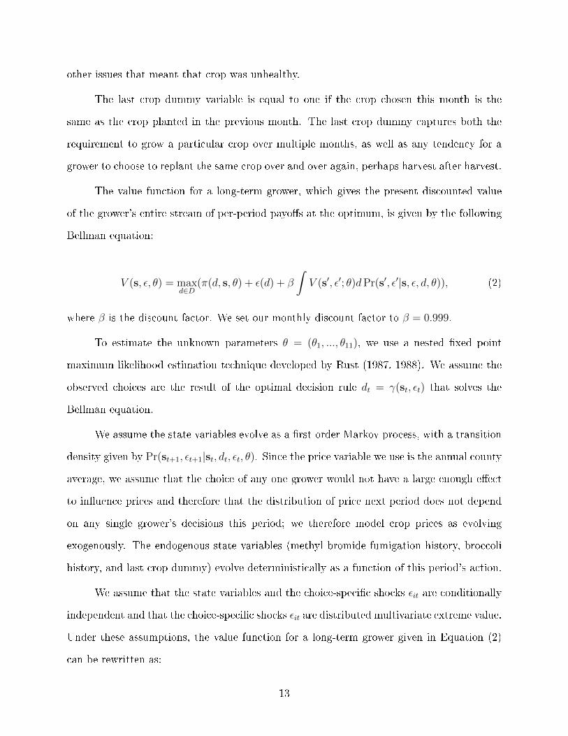
The value function for a long-term grower, which gives the present discounted value

of the grower's entire stream of per-period payo�s at the optimum, is given by the following

Bellman equation:

V (s, ε, θ) = maxd∈D

(π(d, s, θ) + ε(d) + β

∫V (s′, ε′; θ)dPr(s′, ε′|s, ε, d, θ)), (2)

where β is the discount factor. We set our monthly discount factor to β = 0.999.

To estimate the unknown parameters θ = (θ1, ..., θ11), we use a nested �xed point

maximum likelihood estimation technique developed by Rust (1987, 1988). We assume the

observed choices are the result of the optimal decision rule dt = γ(st, εt) that solves the

Bellman equation.

We assume the state variables evolve as a �rst-order Markov process, with a transition

density given by Pr(st+1, εt+1|st, dt, εt, θ). Since the price variable we use is the annual county

average, we assume that the choice of any one grower would not have a large enough e�ect

to in�uence prices and therefore that the distribution of price next period does not depend

on any single grower's decisions this period; we therefore model crop prices as evolving

exogenously. The endogenous state variables (methyl bromide fumigation history, broccoli

history, and last crop dummy) evolve deterministically as a function of this period's action.

We assume that the state variables and the choice-speci�c shocks εit are conditionally

independent and that the choice-speci�c shocks εit are distributed multivariate extreme value.

Under these assumptions, the value function for a long-term grower given in Equation (2)

can be rewritten as:

13

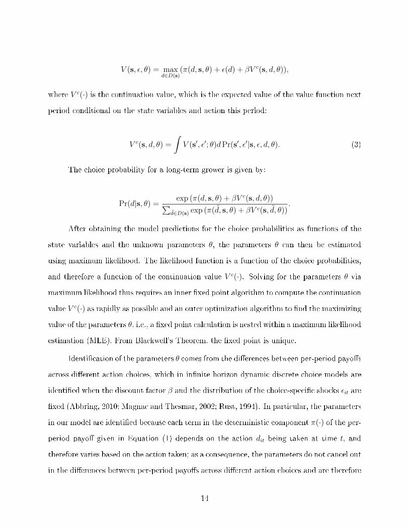
V (s, ε, θ) = maxd∈D(s)

(π(d, s, θ) + ε(d) + βV c(s, d, θ)),

where V c(·) is the continuation value, which is the expected value of the value function next

period conditional on the state variables and action this period:

V c(s, d, θ) =

∫V (s′, ε′; θ)dPr(s′, ε′|s, ε, d, θ). (3)

The choice probability for a long-term grower is given by:

Pr(d|s, θ) = exp (π(d, s, θ) + βV c(s, d, θ))∑d̃∈D(s) exp (π(d̃, s, θ) + βV c(s, d̃, θ))

.

After obtaining the model predictions for the choice probabilities as functions of the

state variables and the unknown parameters θ, the parameters θ can then be estimated

using maximum likelihood. The likelihood function is a function of the choice probabilities,

and therefore a function of the continuation value V c(·). Solving for the parameters θ via

maximum likelihood thus requires an inner �xed point algorithm to compute the continuation

value V c(·) as rapidly as possible and an outer optimization algorithm to �nd the maximizing

value of the parameters θ, i.e., a �xed point calculation is nested within a maximum likelihood

estimation (MLE). From Blackwell's Theorem, the �xed point is unique.

Identi�cation of the parameters θ comes from the di�erences between per-period payo�s

across di�erent action choices, which in in�nite horizon dynamic discrete choice models are

identi�ed when the discount factor β and the distribution of the choice-speci�c shocks εit are

�xed (Abbring, 2010; Magnac and Thesmar, 2002; Rust, 1994). In particular, the parameters

in our model are identi�ed because each term in the deterministic component π(·) of the per-

period payo� given in Equation (1) depends on the action dit being taken at time t, and

therefore varies based on the action taken; as a consequence, the parameters do not cancel out

in the di�erences between per-period payo�s across di�erent action choices and are therefore

14

identi�ed. For example, the coe�cient θ1 on the spinach dummy is identi�ed in the di�erence

between the per-period payo� from choosing to plant spinach and the per-period payo� from

any action choice dit that does not involve planting spinach.11

Standard errors are formed by a nonparametric bootstrap. Fields are randomly drawn

from the data set with replacement to generate 100 independent panels each with the same

number of �elds as in the original data set. The structural model is run on each of the

new panels. The standard errors are then formed by taking the standard deviation of the

parameter estimates from each of the panels.

5 Data

We use Pesticide Use Reporting (PUR) data from the California Department of Pesticide

Regulation.12 Our data set is composed of all �elds in Monterey County on which any

regulated pesticide was applied in the years 1993 to 2011, inclusive.13 Additional data on

prices, yields, and acreage come from the Monterey Agricultural Commissioner's O�ce. We

collapse the data set into monthly observations.

We group the crops into six categories: susceptible (which includes artichoke, strawber-

ries, and cabbage, but excludes lettuce which we represent separately), resistant (cauli�ower

and celery), lettuce, spinach, broccoli, and other.14 From these, we form nine action choices:

susceptible, susceptible with recent fumigation, resistant, broccoli, broccoli with recent fu-

migation, lettuce, lettuce with recent fumigation, spinach, and other.15

11To identify the constant θ11, we normalize the deterministic component π(·) of the per-period payo�from choosing "other" to 0.

12For more information see: http://www.cdpr.ca.gov/docs/pur/purmain.htm.13We use the �eld identi�er as as well as the section, township, and range data from the PUR data set

to match �elds across time. We delete a small number of observations that are non-agricultural uses (golfcourses, freeway sidings, etc.).

14To make the model manageable, we include only the most common crops in Monterey County and thosethat are most often grown in rotation with lettuce. The crops explicitly included in our model account fornearly 90% of the observations. We account for the many rarely planted crops by including an "other" option,which includes various herbs, berries, nursery products, nuts, wine grapes, livestock, and many others.

15The data contain the crop planted in each �eld for each recorded pesticide application. Although the

15

For control options, we use recent histories for broccoli and methyl bromide because

their e�ects on microsclerotia are relatively short-lived. Microsclerotia levels rebound within

one to two seasons, or approximately one year. Thus, broccoli history is the number of

months broccoli was planted in the last 12 months, and methyl bromide history is the

number of months methyl bromide was used in the last 12 months.

The vast majority of �elds (94% of observations) in our data set have only one grower

over the entire time period. Of these, we analyze those long-term growers who appear in

the data on from 1994 to 2010, and we model their decision-making as an in�nite horizon

problem. This data set on long-term growers consists of 615 �elds, each over seventeen years.

We use a marketing year average price for each crop16 to represent growers' expectations

about prices for each year. The marketing year average price is in units of dollars per acre,

and therefore measures revenue per acre and incorporates yield.17 Using the current year's

marketing year average price assumes that growers have rational expectations about what

focus of our research is on methyl bromide, the other pesticides provide observations regarding which cropsare in the ground at which times. Due to the nature of the data, sometimes we do not observe the entireproduction cycle of a crop. For example, strawberries are often in the ground for a year or more; however, ifthere is no registered pesticide applied in one of those months, a gap in the production cycle may appear inour data. We account for this issue in several ways. As long as the missing data are missing for exogenousreasons, missing data will not bias the results. Since there are no pesticide treatments for V. wilt once cropsare in the ground, we have reason to believe that missing months mid-production cycle due to no pesticideapplication in that month are exogenous to the impact of V. wilt on crop and methyl bromide fumigationchoice. We compared the distribution of these months between short-term and long-term growers and �ndthat they are similar distributions. Finally, in the simulations, we simulate all months in the time period, butonly count grower-months that are present in the actual data when calculating welfare and other statisticsfor comparison purposes.

16For lettuce, we use a weighted average of the prices for head and leaf lettuce. In the early years of thedata set, romaine and other types of lettuce were not broken out separately, so gross revenue numbers varybased on this reporting, but do not a�ect the discretized value of the price.

17We look at gross revenue rather than net revenue due to data limitations. Costs are captured by ourcrop-fumigation dummies and our constant. Estimating net revenue did not improve the overall model, andcost di�erences among crops are mainly driven by methyl bromide fumigation, which is explicitly includedin the model, and/or the di�erence between strawberry costs compared to other crops. Strawberry costs aregenerally an order of magnitude higher than for the vegetable crops, in part due to fumigation cost accordingto Richard Smith, Farm Advisor for Vegetable Crop Production & Weed Science with the University ofCalifornia Cooperative Extension in Monterey County. We also attempted to incorporate this e�ect byincluding dummy variables for the di�erent crop choices and fumigation, with resistant crops as the baseline.Unsurprisingly, the susceptible dummy variables (which includes strawberries) was collinear with the methylbromide fumigation variable; we therefore do not include the susceptible crop dummy variable in our model.We expect the crop-fumigation dummies to at least partially capture the cost di�erences among the di�erentcrops.

16

the average marketing year price will be that year.18 The Monterey County Agricultural

Commissioner's O�ce publishes annual crop reports including prices, yields harvest, and

acreages for major crops in the county. Monterey County is a major producer of many of

the crops included in our model. For most crops, these prices are highly correlated with

California-wide price data published by the National Agricultural Statistics Service. We

discretize the marketing year average price into 6 bins; the marketing year average price bins

are shown in Figure 1.

We combine the marketing year average price data with data on the timing of harvests

for various crops in Monterey. For each crop, the harvest month dummy variable for that

crop is equal to one in months during which that crop may be harvested, and zero in months

during which that crop is not harvested (i.e., winter months for most crops).19 For all crops,

we have observations during the winter months, including crops that have just been planted

and are not yet ready for harvest, and crops such as strawberries that overwinter for harvest

in the coming year.

Summary statistics for the state variables for long-term growers are in Table 1. The

mean discretized price for broccoli is relatively low, a�rming that broccoli is a low-return

crop. Spinach is a relatively small portion of the acreage grown in Monterey County, ap-

proximately a tenth of the size of the acreage planted to lettuce according to the most recent

Monterey County Crop Report.

Figure 2 plots the actual fraction of grower-months in each action type for the long-

term growers. As seen in Figure 2, lettuce accounts for over 60% of the grower-months for

these long-term growers. Figure 3 plots the actual fraction of grower-months in each action

by month of year. The actual fraction of grower-months in each action varies by the month

18Instead of rational expectations about price, another possible assumption is that growers' best guessfor this year's price is last year's price. The results are robust to whether we use lagged prices rather thancurrent prices (Carroll et al., 2017a).

19There is a separate harvest month dummy variable for each crop-month. These data come from RichardSmith, Farm Advisor for Vegetable Crop Production & Weed Science with the University of CaliforniaCooperative Extension in Monterey County.

17

of the year, with lettuce predominant in the spring and summer months, and other and

susceptible crops having the highest proportion in the winter months. Figure 4 plots the

actual fraction of grower-months in each action type over the years. The proportions are

relatively constant across years.

6 Results

The results for long-term growers are presented in Table 2. We run our model on 3 di�erent

time periods: the entire time period of our data set (àll'), the early half of the data prior

to 2001 (èarly'), and the later half of the data from 2001 to 2011 (`late'). We report our

estimates for the parameters in the per-period payo� function in Equation (1). The payo�s

do not have units because price is discretized and therefore no longer in dollars. Since we do

not have units for payo�s, we can compare only relative payo�s and welfare.

According to the results, the coe�cient on the spinach dummy is signi�cant and neg-

ative, suggesting that planting spinach is undesirable for reasons that are not fully captured

by its price.20 This coe�cient provides evidence that V. wilt is a problem, since it is likely

due to the fact that spinach is associated with V. wilt that spinach is undesirable.21

The coe�cient on methyl bromide in the current period is signi�cant and negative,

which means there is a cost to methyl bromide that may yield future bene�t to either the

current crop or a future crop. The coe�cient is more negative in the later half of the

data, likely because the Montreal Protocol started to limit the legal availability of methyl

bromide during this period (California Department of Pesticide Regulation, 2010; United

20Because price is the discretized marketing average price of spinach per acre, the price measures revenueper acre, and therefore incorporates yield as well. Thus, the signi�cant negative coe�cient on the spinachdummy suggests that spinach is not desirable to plant for reasons that are not fully captured by its price,yield, or revenue per acre.

21One may worry that the negative coe�cient on the spinach dummy is possibly also consistent with aproblem in modeling where the other crops with longer crop cycles would potentially be more appealingthan spinach. However, even when returns are divided by the length of season, the returns to spinach versusother crops still follow the same order. This result suggests that the season length is not the driving factorbehind this coe�cient. We con�rm in Carroll et al. (2017a) that the signi�cant negative coe�cient on thespinach dummy is robust to whether we divide returns by season length.

18

States Environmental Protection Agency, 2012b), and also because there is more demand

for methyl bromide in the later half of the data set when V. wilt became more of a problem,

resulting in a higher price for using methyl bromide.

The broccoli dummy coe�cient is negative, but not signi�cant, suggesting that planting

broccoli is not as desirable as planting lettuce (since the lettuce dummy has a signi�cant

positive coe�cient) and requires foregoing current bene�ts (or incurring current costs) for

future gain.

The coe�cient on the interaction term between lettuce and methyl bromide history is

signi�cant and positive in the later half of the time period, suggesting that methyl bromide

is an e�ective control option in the later period. Similarly, the coe�cient on the interaction

term between lettuce and broccoli history is signi�cant and positive, which suggests that

planting broccoli is also an e�ective control option.

Although the coe�cient on the spinach dummy and methyl bromide history interaction

term is not signi�cant, the point estimate is positive and smaller in magnitude than the

spinach dummy coe�cient, suggesting that the undesirability of spinach is mitigated by

having methyl bromide history. In addition to the signi�cant positive coe�cient on the

lettuce and methyl bromide interaction in the later period, this further suggests that methyl

bromide is an e�ective control option in the later period.

Similarly, although the coe�cient on the spinach dummy and broccoli history interac-

tion term is not signi�cant, the point estimate is positive and smaller in magnitude than the

spinach dummy, also suggesting that the undesirability of spinach is mitigated by broccoli

history. In addition to the signi�cant positive coe�cient on the lettuce and broccoli history

interaction, this further suggests that planting broccoli is an e�ective control option.

The lettuce dummy has a signi�cant positive coe�cient, which means that owners

derive bene�ts from planting lettuce beyond its price, such as meeting shipper contract

requirements.22 Thus, it is desirable for growers to control V. wilt, since they bene�t from

22In the model, returns are estimated at the county level, so although contracts can and do specify prices,

19

planting lettuce.

The coe�cient on price at the time of harvest is negative. At �rst blush this may

appear counterintuitive, as economic theory predicts that price will have a positive e�ect

on return. After looking further into the data, however, the reason for this result becomes

more clear. Strawberries have a much higher revenue per acre than any of the vegetable

crops included in this data set, on the order of $70,000 for strawberries versus $20,000 or less

for some vegetable crops. Most growers concentrate on either strawberry crops or vegetable

crops, so there are very few cases in the data of growers switching to strawberries from

vegetable crops, even though that behavior is what one would expect based on price alone.

When strawberries are removed as an action choice in the analysis, the coe�cient for price is

then positive. In addition, some strawberry growers are switching to contracts in which the

price plays very little role in determining their pro�t. They are paid a baseline amount for

growing the crop and may make more money in a particularly good year, but do not bear

the downside risk in a poor year.

The negative coe�cient on price at the time of harvest therefore suggests that there

may be something partially driving growers' decision-making that is not observable. For

example, growers may have connections and contracts that tie them to certain crops that

we cannot observe. They may have expertise or risk pro�les that better suit certain crops.

Perhaps some growers consider themselves vegetable growers and the cost of switching to

strawberries is too high. Uncertainty related to the future of methyl bromide and its lack of

suitable replacements for treating V. wilt could also play a role. Unobservable factors that

may make growers less likely to switch crops are at least partially captured in our model by

the last crop dummy. We hope to explore these issues further in future work.

The coe�cient on the last crop dummy is signi�cant and positive, which suggests that

growers are committed to previous crops, which is also consistent with the hypothesis that

growers do not switch crops often and therefore are less responsive to price.

we expect the return used in the model to be exogenous to contracting decisions.

20

The total average e�ects of the variables that appear in more than one term of the

per-period payo� function are reported at the bottom of Table 2. The spinach dummy has a

total average e�ect that is signi�cant and negative on net, which provides evidence that V.

wilt is a problem, even if the undesirability of spinach is mitigated by having methyl bromide

history and/or broccoli history.

The lettuce dummy has a signi�cant and positive total average e�ect, which means

that owners derive bene�ts from planting lettuce beyond its price, and that the bene�ts

of lettuce are enhanced in the presence of control options such as methyl bromide history

and/or broccoli history.

Methyl bromide history has a positive total average e�ect that is signi�cant in the

later half of the time period, suggesting that methyl bromide is an e�ective control option

in the later period. Similarly, broccoli history has a signi�cant and positive total average

e�ect, suggesting that planting broccoli is an e�ective control option.

In using a marketing year average price for each crop to represent growers' expectations

about prices for each year, we assume that growers have rational expectations about the price.

Instead of rational expectations about price, another possible assumption is that growers'

best guess for this year's price is last year's price. The results are robust to whether we use

lagged prices rather than current prices (Carroll et al., 2017a).

We choose not to model the grower as only receiving the revenue for his crop the �rst

month of the harvest season, as this would not explain why growers may plant the same crop

for multiple months in the harvest season. Staying in the harvest season longer sometimes

yields higher revenue because it enables the grower to harvest more product or replant the

crop for more harvest, both of which are better captured by having the grower receive more

revenue if he stays in the harvest season longer. For similar reasons, we choose not to model

the grower as only receiving the revenue for his crop the last month of the harvest season.

As seen in Carroll et al. (2017a), we �nd that the results are robust to whether we divide

the marketing year average price for each crop by its average harvest season length, and

21

therefore to whether we assume growers who plant the same crop for multiple months in a

harvest season receive more revenue than those who plant that crop for only one month in

the harvest season.

We calculate the normalized average grower welfare per grower per month for the entire

time period (àll'), the early time period (èarly'), and the later time period (`late'). The

welfare is calculated as the present discounted value of the entire stream of payo�s to growers

evaluated at the parameter values, summed over all growers in the relevant data set, then

divided by the number of grower-months in the relevant data set. The average grower welfare

per grower per month is then normalized so that the average welfare per grower per month

over the entire time period (àll') is 100.

The standard errors for the welfare values are calculated using the parameter estimates

from each of 100 bootstrap samples. For each of the 100 bootstrap samples, we calculate the

average welfare per grower per month using the parameter estimates from that bootstrap

sample, and normalize it. The standard error of the normalized welfare is the standard

deviation of the normalized welfare over all 100 bootstrap samples.

The welfare results are presented in Table 3. According to the welfare results, average

grower welfare per grower-month is higher in the earlier time period than in the later time

period, perhaps because V. wilt became more of a problem in the later time period.

7 Simulations

We use the estimated parameters from our dynamic structural model to simulate the e�ects

of crop disease on agricultural productivity. In particular, we use counterfactual simulations

to analyze the e�ects of V. wilt on crop-fumigation decisions and on grower welfare.

The severity of the crop disease is measured by the coe�cient θ1 on the spinach dummy

in the grower's per-period payo� function. The spinach dummy coe�cient captures the

e�ects of spinach on payo�s that are not internalized in spinach price. The more negative

22

the spinach dummy coe�cient θ1, the more severe the disease.

To analyze the e�ects of crop disease on agricultural productivity, we use the estimated

parameters from our dynamic structural model in Section 6 to simulate how di�erent values

of the spinach dummy coe�cient would a�ect the choices and payo�s of growers. According

to the results of the dynamic structural model for growers in Table 2, the coe�cient θ1 on

the spinach dummy when we use data over the entire time period (àll') is -1.1311.

We consider a set of twenty-one evenly spaced values of the spinach dummy coe�cient

θ1 between -2.00 and 0.00. A spinach dummy coe�cient θ1 of -2.00 represents a scenario in

which V. wilt is even more severe than it currently is, and therefore one in which spinach

seeds have an even greater negative e�ect on grower payo�s than they currently do. A

spinach dummy coe�cient θ1 equal to zero represents a scenario in which V. wilt is no longer

an economically damaging disease, and therefore one in which the e�ect of spinach on grower

payo�s (aside from price e�ects) is neutral and not economically signi�cant.

For each possible value of the spinach dummy coe�cient θ1, we run 100 simulations

of the choices and payo�s that would arise if the spinach dummy coe�cient were equal that

values. For each of the 100 simulations, we calculate the average grower welfare per month,

which is the total welfare divided by the number of grower-months. Then, for each possible

value of the spinach dummy coe�cient, we average the grower welfare per month over the

100 simulations using that value of the spinach dummy coe�cient. We then calculate the

average bene�ts to the grower from mitigating the disease taking the average grower welfare

per month at each value of the spinach dummy coe�cient, and then subtracting the average

grower welfare per month when the spinach dummy coe�cient θ1 is an extremely severe

-2.00. In other words, we normalize the average grower welfare per month when the spinach

dummy coe�cient θ1 is an extremely severe -2.00 to 0.

Standard errors are calculated using a nonparametric bootstrap. In particular, we

calculate the standard errors of the grower bene�ts from disease mitigation using the pa-

rameter estimates from each of twenty-�ve bootstrap samples. For each of the twenty-�ve

23

bootstrap samples, we run twenty-�ve simulations using the parameter estimates from that

bootstrap sample.23 The standard error of the grower bene�ts is the standard deviation of

the respective statistic over all twenty-�ve bootstrap samples.

Figure 5 plots the bene�ts to a grower per month from mitigating the disease, averaged

over 100 simulations, as a function of the coe�cient θ1 on the spinach dummy achieved.

According to our results, the bene�ts to the growers are the highest when the coe�cient

on spinach is driven up to zero, which represents the scenario in which V. wilt is no longer

an economically damaging disease. As the coe�cient on spinach becomes more negative

(representing scenarios in which V. wilt is more severe a disease), the bene�ts to growers

decline.

To analyze the e�ects of mitigating V. wilt on crop-fumigation decisions, we simulate

the crop choices of long-term growers when the spinach dummy coe�cient θ1 is equal to

-1.00, which represents the scenario in which V. wilt is less severe than it currently is; and

when the spinach dummy coe�cient θ1 is equal to zero, which represents the scenario in

which V. wilt is no longer an economically damaging disease.

Standard errors and 95% con�dence intervals are calculated using a nonparametric

bootstrap. In particular, we calculate the standard errors of the simulation statistics (e.g.,

mean fraction of grower-months in each action) using the parameter estimates from each of

twenty-�ve bootstrap samples. For each of the twenty-�ve bootstrap samples, we run twenty-

�ve simulations using the parameter estimates from that bootstrap sample.24 The standard

error of the simulation statistics (e.g., mean fraction of grower-months in each action) is the

standard deviation of the respective statistic over all twenty-�ve bootstrap samples.

23Constraints on computational time preclude us from running the twenty-�ve simulations per bootstrapsample for more than twenty-�ve bootstrap samples per scenario. When we calculated the standard errorfor welfare for scenario 1 using 100 bootstrap samples instead of twenty-�ve bootstrap samples, the value ofthe standard errors were similar using both twenty-�ve bootstrap samples and 100 bootstrap samples.

24Constraints on computational time preclude us from running the twenty-�ve simulations per bootstrapsample for more than twenty-�ve bootstrap samples per scenario. When we calculated the standard errorfor welfare for scenario 1 using 100 bootstrap samples instead of twenty-�ve bootstrap samples, the value ofthe standard errors were similar using both twenty-�ve bootstrap samples and 100 bootstrap samples.

24

Figures 6-7 simulate growers crop choices when V. wilt is no longer an economically

damaging disease (θ1 = 0) and when V. wilt is less severe than it currently is (θ1 = −1.00),

respectively. The fraction of grower-months planted to lettuce is higher under both scenarios

than they are in the actual data in Figure 2. Thus, when V. wilt is less severe, growers plant

more lettuce, likely because V. wilt then becomes less of a problem.

Figures 8-9 show the fraction of grower-months in each action type by month of year

when V. wilt is no longer an economically damaging disease (θ1 = 0) and when V. wilt is less

severe than it currently is (θ1 = −1.00), respectively. Compared to Figure 3, which shows

the actual data, the results of the simulations of less severe disease show more grower-months

planted to lettuce, especially in the last months of the year when the actual data consists

more of susceptible and other crops.

Figures 10-11 show the fraction of grower months in each action type by year when V.

wilt is no longer an economically damaging disease (θ1 = 0) and when V. wilt is less severe

than it currently is (θ1 = −1.00), respectively. Compared to Figure 4, which shows the actual

data, the results of the simulations of less severe disease show more grower-months planted

to lettuce and fewer grower-months planted to other crops. Thus, when the disease is less

severe, growers plant more lettuce, likely because V. wilt then becomes less of a problem.

8 Conclusion

This paper discusses the e�ects on agricultural productivity of Verticillium dahliae, a soil

borne fungus that is introduced to the soil via infested spinach seeds and that causes lettuce

to be a�icted with V. wilt. We use a dynamic structural econometric model of V. wilt

management for lettuce crops in Monterey County, California to examine the e�ects of V.

wilt on crop-fumigation decisions and on grower welfare.

According to our results, planting spinach is undesirable for reasons that are not fully

captured by its price, which is consistent with the conclusion that V. wilt is a problem.

25

Fumigating with methyl bromide and planting broccoli are both e�ective control options,

but involve incurring costs or foregoing pro�t in the current period for future bene�t. We

�nd that average grower welfare per grower-month is higher in the earlier time period than

in the later time period, perhaps because V. wilt became more of a problem in the later time

period.

According to the results of our counterfactual simulations of the e�ects of V. wilt on

agricultural productivity, the bene�ts to the growers are the highest when the coe�cient

on spinach is equal to zero, which represents the scenario in which V. wilt is no longer

an economically damaging disease. As the coe�cient on spinach becomes more negative

(representing scenarios in which V. wilt is more severe a disease), the bene�ts to growers

decline. When the disease is less severe, growers plant more lettuce, likely because V. wilt

then becomes less of a problem. Thus, V. wilt has important e�ects on crop-fumigation

decisions, grower welfare, and agricultural productivity.

There are two main externalities that arise due to V. wilt, and that have important

implications for agricultural productivity. The �rst externality is an intertemporal exter-

nality. When faced with managing a disease that requires future investment, short- and

long-term decision-makers may have di�erent incentives and choose to manage the disease

di�erently. In the case of V. wilt, because the options for controlling V. wilt require long-

term investments for future gain, an intertemporal externality arises with short-term growers,

who are likely to rent the land for only a short period of time. Renters, therefore, might not

make the long-term investments needed to control V. wilt. As a consequence, future renters

and the landowner may su�er from decisions of previous renters not to invest in control

options. Thus, decisions made by current renters impose an intertemporal externality on

future renters and the landowner.

In Carroll et al. (2017a), we analyze the factors that a�ect crop choice and fumigation

decisions made by growers and consider how the decisions of long-term growers (whom we

call �owners�) di�er from those of short-term growers (whom we call �renters�). We examine

26

whether existing renter contracts internalize the intertemporal externality that a renter's

decisions today impose on future renters and the landowner, and analyze the implications of

renting versus owning land on welfare.

Although contracts can be a potential method for internalizing an externality between

di�erent parties, our empirical results in Carroll et al. (2017a) show that existing rental

contracts do not fully internalize the intertemporal externality imposed by renters on future

renters and the landowner. This outcome may be because of the relatively recent development

of the disease and knowledge of its causes, more restrictive contracts not being the norm, the

possibility of land unknowingly being contaminated before rental, or di�culty in enforcing or

monitoring aspects of the contract such as whether boots and equipment are washed between

�elds.

In addition to the intertemporal externality, a second externality that arises due to V.

wilt is a supply chain externality between companies selling spinach seed and growers who

may lettuce. Growers wish to protect their �elds from V. wilt, but they cannot easily prevent

introduction of the disease by spinach seeds when spinach is planted without incurring testing

costs and cleaning fees. Currently, seed companies are unwilling to test or clean spinach seeds,

especially as spinach producers are not a�ected by this disease. Thus, decisions made by

seed companies regarding whether and how much to test or clean spinach seeds impose a

supply chain externality on growers.

In Carroll et al. (2017b), we analyze the supply chain externality between growers and

seed companies. We calculate the bene�ts to growers from testing and cleaning spinach seed

by simulating growers' optimal decisions and welfare under di�erent levels of seed testing

and cleaning. We then estimate the spinach seed company's cost to testing and cleaning

spinach seeds in order to reduce the level of microsclerotia, and compare the spinach seed

company's cost to the grower's bene�ts. Because seed cleaning cost data are not available,

we use several functional forms and parameters to estimate potential cost functions. We

then use the bene�ts and costs to determine the welfare maximizing level of seed testing and

27

cleaning.

According to our results in Carroll et al. (2017b), using data over the entire time

period, we �nd that a cooperative solution would increase welfare, and in most cases, a

cooperative solution would require that the spinach seed company engage in more spinach

seed testing and cleaning than in the status quo. Our work regarding the supply chain

externality between seed companies and growers sheds light on how treatment of spinach

seeds could potentially reduce externalities between seed companies and growers.

Crop diseases and how they are managed can have a large impact on agricultural

productivity. Externalities due to V. wilt that arise with renters, and between seed companies

and growers have important implications for the management of V. wilt in particular, and

also for the management of diseases in agriculture in general.

28

References

Abbring, J. 2010. �Identi�cation of Dynamic Discrete Choice Models.� Annual Review of

Economics 2:367�394.

Aguirregabiria, V., and A. Luengo. 2016. �A Microeconometric Dynamic Structural Model

of Copper Mining Decisions.� Working Paper, Available <http://aguirregabiria.net/

wpapers/copper_mining.pdf>.

Atallah, S., M. Gomez, J. Conrad, and N. JP. 2015. �A Plant-Level, Spatial, Bioeconomic

Model of Plant Disease, Di�usion, and Control: Grapevine Leafroll Disease.� American

Journal of Agricultural Economics 97:199�218.

Atallah, Z., R. Hayes, and K. Subbarao. 2011. �Fifteen Years of Verticillium Wilt of Lettuce

in America's Salad Bowl: A Tale of Immigration, Subjugation, and Abatement.� Plant

Disease 95:784�792.

Atallah, Z., K. Maruthachalam, L. Toit, S. Koike, R. Michael Davis, S. Klosterman, R. Hayes,

and K. Subbarao. 2010. �Population Analyses of the Vascular Plant Pathogen Verticillium

dahliae Detect Recombination and Transcontinental Gene Flow.� Fungal Genetics and

Biology 47:416�422.

California Department of Pesticide Regulation. 2010. �Department of Pesticide Regulation

Announces Work Group to Identify Ways to Grow Strawberries without Fumigants.� Avail-

able <http://www.cdpr.ca.gov/docs/pressrls/2012/120424.htm>.

Carlson, G.A., and C.E. Main. 1976. �Economics of Disease-Loss Management.� Annual

Review of Phytopathology 14:381�403.

Carroll, C.L., C.A. Carter, R.E. Goodhue, and C.-Y. C. Lin Lawell. 2017a. �The Economics

of Decision-Making for Crop Disease Control.� Working Paper, University of California at

Davis.

29

�. 2017b. �Supply Chain Externalities and Agricultural Disease.� Working Paper, University

of California at Davis.

De Pinto, A., and G.C. Nelson. 2009. �Land Use Change with Spatially Explicit Data: A

Dynamic Approach.� Environmental and Resource Economics 43:209�229.

du Toit, L., M. Derie, and P. Hernandez-Perez. 2005. �Verticillium Wilt in Spinach Seed

Production.� Plant Disease 89:4�11.

du Toit, L., and P. Hernandez-Perez. 2005. �E�cacy of Hot Water and Chlorine for Eradi-

cation of Cladosporium variabile, Stemphylium botryosum, and Verticillium dahliae from

Spinach Seed.� Plant Disease 89:1305�1312.

Duressa, D., G. Rauscher, S.T. Koike, B. Mou, R.J. Hayes, K. Maruthachalam, K.V. Sub-

barao, and S.J. Klosterman. 2012. �A Real-Time PCR Assay for Detection and Quanti�-

cation of Verticillium dahliae in Spinach Seed.� Phytopathology 102:443�451.

Fradin, E.F., and B.P.H.J. Thomma. 2006. �Physiology and Molecular Aspects of Verticillium

Wilt Diseases Caused by V. dahliae and V. albo-atrum.� Molecular Plant Pathology 7:71�

86.

Gomez, M.I., H.M. Nunez, and H. Onal. 2009. �Economic Impacts of Soybean Rust on the

US Soybean Sector.� 2009 Annual Meeting, July 26-28, 2009, Milwaukee, Wisconsin No.

49595, Agricultural and Applied Economics Association.

Hueth, D., and U. Regev. 1974. �Optimal Agricultural Pest Management with Increasing

Pest Resistance.� American Journal of Agricultural Economics 56:543�552.

IPC. 2003. �International Phytosanitary Certi�cate No. 4051.�

Johansson, R.C., M. Livingston, J. Westra, and K.M. Guidry. 2006. �Simulating the U.S. Im-

pacts of Alternative Asian Soybean Rust Treatment Regimes.� Agricultural and Resource

Economics Review 35:116�127.

30

Lin Lawell, C.-Y. C. 2017. �Wind Turbine Shutdowns and Upgrades in Denmark: Timing

Decisions and the Impact of Government Policy.� Working Paper, University of California

at Davis.

Magnac, T., and D. Thesmar. 2002. �Identifying Dynamic Discrete Choice Processes.� Econo-

metrica 70:801�816.

Maruthachalam, K., S.J. Klosterman, A. Anchieta, B. Mou, and K.V. Subbarao. 2013. �Col-

onization of Spinach by Verticillium dahliae and E�ects of Pathogen Localization on the

E�cacy of Seed Treatments.� Phytopathology 103:268�280.

McKee, G.J., R.E. Goodhue, F.G. Zalom, C.A. Carter, and J.A. Chalfant. 2009. �Population

Dynamics and the Economics of Invasive Species Management: The Greenhouse White�y

in California-Grown Strawberries.� Journal of Environmental Management 90:561�570.

Mo�tt, L., D. Hall, and C. Osteen. 1984. �Economic Thresholds Under Uncertainty with

Application to Corn Nematode Management.� Southern Journal of Agricultural Economics

16:151�157.

Monterey County Agricultural Commissioner. 2015. �Crop Reports and Eco-

nomic Contributions.� Available <http://www.co.monterey.ca.us/government/

departments-a-h/agricultural-commissioner/forms-publications/

crop-reports-economic-contributions>.

National Agricultural Statistics Service. 2015. �California Agricultural Statistics:

2013 Crop Year.� Available <http://www.nass.usda.gov/Statistics_by_State/

California/Publications/California_Ag_Statistics/index.asp>.

Noailly, J. 2008. �Coevolution of Economic and Ecological Systems.� Journal of Evolutionary


31

Palm, M.E. 2001. �Systematics and the Impact of Invasive Fungi on Agriculture in the United

States.� BioScience 51:141�147.

Rapson, D. 2014. �Durable Goods and Long-run Electricity Demand: Evidence from Air

Conditioner Purchase Behavior.� Journal of Environmental Economics and Management

68:141�160.

Rossman, A. 2009. �The Impact of Invasive Fungi on Agricultural Ecosystems in the United

States.� Biological Invasions 11:97�107.

Rothwell, G., and J. Rust. 1997. �On the Optimal Lifetime of Nuclear Power Plants.� Journal

of Business & Economic Statistics 15:195�208.

Rust, J. 1988. �Maximum Likelihood Estimation of Discrete Control Processes.� SIAM Jour-

nal on Control and Optimization 26:1006�1024.

�. 1987. �Optimal Replacement of GMC Bus Engines: An Empirical Model of Harold

Zurcher.� Econometrica: Journal of the Econometric Society 55:999�1033.

�. 1994. �Structural Estimation of Markov Decision Processes.� In R. Engle and D. McFad-

den, eds. Handbook of Econometrics . Amsterdam: North-Holland, vol. 4, pp. 3081�3143.

Scott, P.T. 2013. �Dynamic Discrete Choice Estimation of Agricultural Land Use.� Working

Paper, Available <http://www.ptscott.com>.

Shetty, K., K. Subbarao, O. Huisman, and J. Hubbard. 2000. �Mechanism of Broccoli-

Mediated Verticillium Wilt Reduction in Cauli�ower.� Phytopathology 90:305�310.

Short, D.P.G., S. Gurung, S.T. Koike, S.J. Klosterman, and K.V. Subbarao. 2015. �Frequency

of Verticillium Species in Commercial Spinach Fields and Transmission of V. dahliae from

Spinach to Subsequent Lettuce Crops.� Phytopathology 105:80�90.

32

Subbarao, K.V., and J.C. Hubbard. 1996. �Interactive E�ects of Broccoli Residue and Tem-

perature on Verticillium dahliae Microsclerotia in Soil and on Wilt in Cauli�ower.� Phy-

topathology 86:1303�1310.

Subbarao, K.V., J.C. Hubbard, and S.T. Koike. 1999. �Evaluation of Broccoli Residue In-

corporation into Field Soil for Verticillium Wilt Control in Cauli�ower.� Plant Disease

83:124�129.

Timmins, C. 2002. �Measuring the Dynamic E�ciency Costs of Regulators' Preferences:

Municipal Water Utilities in the Arid West.� Econometrica 70:603�629.

United States Environmental Protection Agency. 2012a. �Critical Use Exemption Informa-

tion.� Available <http://www.epa.gov/ozone/mbr/cueinfo.html>.

�. 2012b. �The Phaseout of Methyl Bromide.� Available <http://www.epa.gov/ozone/

mbr/index.html>.

van Kooten, G.C., W.P. Weisensel, and D. Chinthammit. 1990. �Valuing Tradeo�s between

Net Returns and Stewardship Practices: The Case of Soil Conservation in Saskatchewan.�

American Journal of Agricultural Economics 72:104�113.

Weisensel, W.P., and G.C. van Kooten. 1990. �Estimation of Soil Erosion Time Paths: The

Value of Soil Moisture and Topsoil Depth Information.� Western Journal of Agricultural


Wu, J. 2001. �Optimal Weed Control Under Static and Dynamic Decision Rules.� Agricultural


Xiao, C., and K. Subbarao. 1998. �Relationships Between Verticillium dahliae Inoculum

Density andWilt Incidence, Severity, and Growth of Cauli�ower.� Phytopathology 88:1108�

1115.

33

Figure 1Marketing year average prices per acre

Note: Black dashed lines delineate the bins used to discretize the marketing year averageprice.

34

Table 1Summary statistics for state variables

Mean Std. Dev. Minimum Maximum

Spinach dummy 0.0285 0.1665 0 1Methyl bromide today dummy 0.0033 0.0577 0 1Broccoli dummy 0.0606 0.2385 0 1Lettuce *Methyl bromide history 0.0229 0.1602 0 3Lettuce *Broccoli history 1.1709 1.8277 0 12Spinach *Methyl bromide history 0.0015 0.0431 0 2Spinach *Broccoli history 0.0397 0.3701 0 10Lettuce today dummy 0.6379 0.4806 0 1Susceptible price*Susceptible harvest 5.0660 1.4914 0 6Resistant price*Resistant harvest 1.8748 1.6125 0 4Broccoli price*Broccoli harvest 1.1742 0.5082 0 2Lettuce price*Lettuce harvest 1.9552 1.1004 0 4Spinach price*Spinach harvest 2.5268 1.4709 0 4Notes: Number of observations: 25,789. For each crop, the harvest month dummy variablefor that crop is equal to one in months during which that crop may be harvested, and zeroin months during which that crop is not harvested (i.e., winter months for most crops).

35

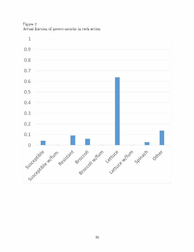
Figure 2Actual fraction of grower-months in each action

36

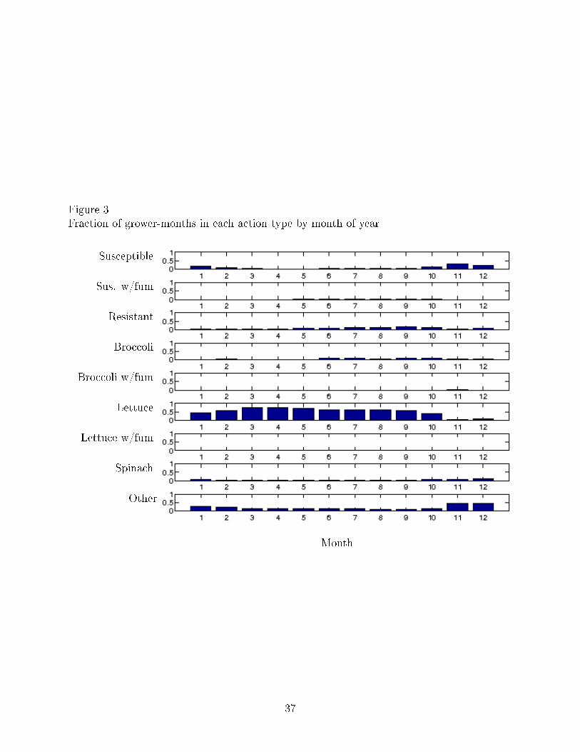
Figure 3Fraction of grower-months in each action type by month of year

Susceptible

Sus. w/fum

Resistant

Broccoli

Broccoli w/fum

Lettuce

Lettuce w/fum

Spinach

Other

Month

37

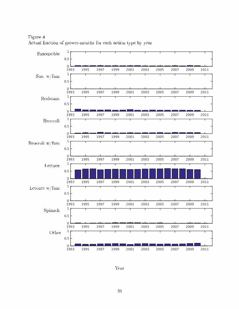
Figure 4Actual fraction of grower-months for each action type by year

Susceptible

Sus. w/fum

Resistant

Broccoli

Broccoli w/fum

Lettuce

Lettuce w/fum

Spinach

Other

Year

38

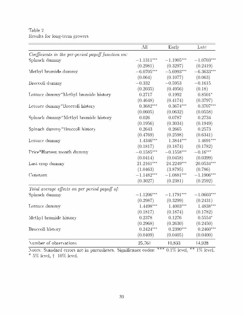
Table 2Results for long-term growers

All Early Late

Coe�cients in the per-period payo� function on:

Spinach dummy −1.1311∗∗∗ −1.1905∗∗∗ −1.0703∗∗∗(0.2981) (0.3297) (0.2419)

Methyl bromide dummy −6.0705∗∗∗ −5.6993∗∗∗ −6.3633∗∗∗(0.064) (0.1077) (0.063)

Broccoli dummy −0.332 −0.5953 −0.1615(0.2035) (0.4956) (0.18)

Lettuce dummy*Methyl bromide history 0.2717 0.1992 0.8501∗

(0.4648) (0.4174) (0.3797)Lettuce dummy*Broccoli history 0.3682∗∗∗ 0.3674∗∗∗ 0.3707∗∗∗

(0.0605) (0.0632) (0.0558)Spinach dummy*Methyl bromide history 0.026 0.0787 0.2734

(0.1956) (0.3034) (0.1949)Spinach dummy*Broccoli history 0.2643 0.2665 0.2573

(0.4769) (0.2598) (0.6341)Lettuce dummy 1.4346∗∗∗ 1.3844∗∗∗ 1.4691∗∗∗

(0.1817) (0.1874) (0.1782)Price*Harvest month dummy −0.1585∗∗∗ −0.1558∗∗∗ −0.16∗∗∗

(0.0414) (0.0458) (0.0399)Last crop dummy 21.2161∗∗∗ 24.2249∗∗∗ 20.0534∗∗∗

(1.0463) (3.8795) (0.786)Constant −1.1482∗∗∗ −1.0881∗∗∗ −1.1906∗∗∗

(0.3027) (0.2381) (0.2592)

Total average e�ects on per-period payo� of:

Spinach dummy −1.1206∗∗∗ −1.1791∗∗∗ −1.0603∗∗∗(0.2987) (0.3299) (0.2431)

Lettuce dummy 1.4498∗∗∗ 1.4003∗∗∗ 1.4838∗∗∗

(0.1817) (0.1874) (0.1782)Methyl bromide history 0.2378 0.1276 0.5554∗

(0.2968) (0.2630) (0.2450)Broccoli history 0.2424∗∗∗ 0.2390∗∗∗ 0.2460∗∗∗

(0.0409) (0.0405) (0.0400)

Number of observations 25,761 10,833 14,928

Notes: Standard errors are in parentheses. Signi�cance codes: ∗∗∗ 0.1% level, ∗∗ 1% level,∗ 5% level, † 10% level.

39

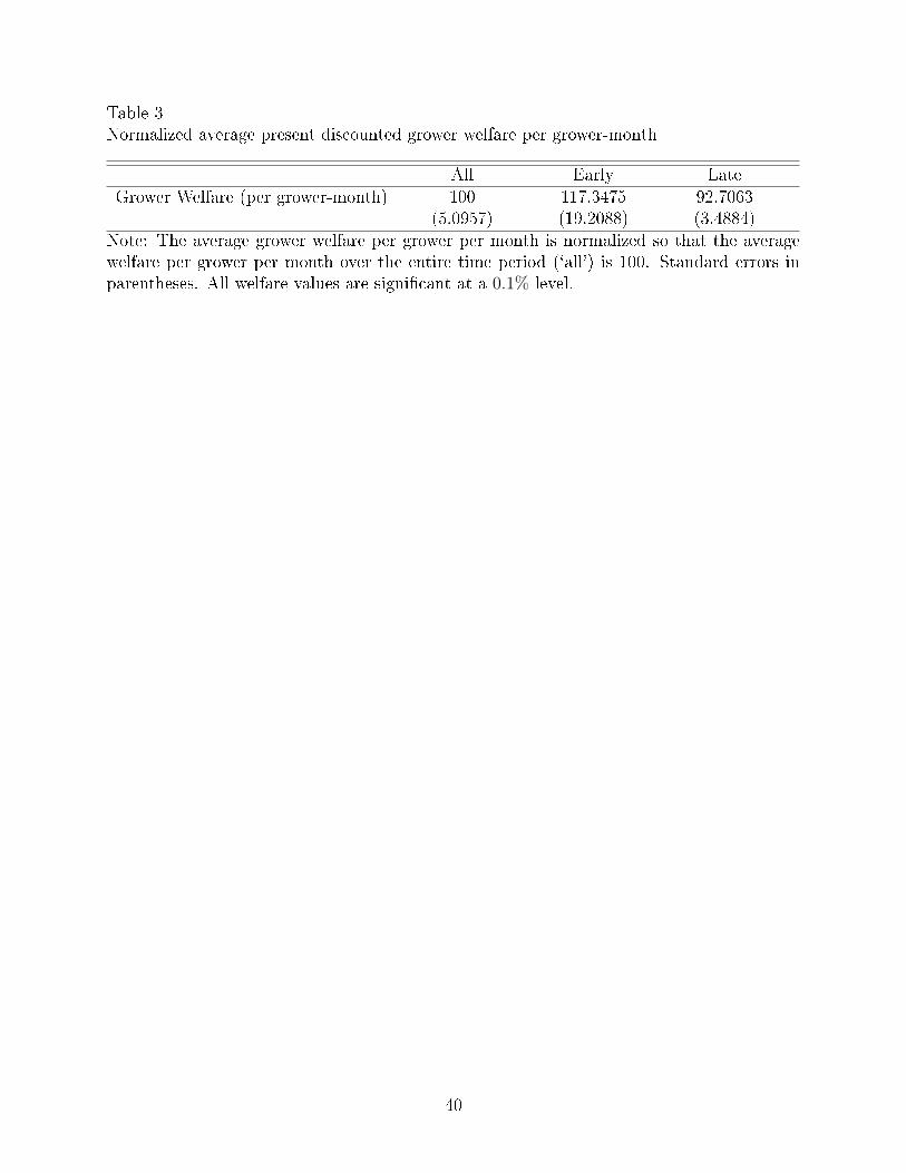
Table 3Normalized average present discounted grower welfare per grower-month

All Early Late

Grower Welfare (per grower-month) 100 117.3475 92.7063(5.0957) (19.2088) (3.4884)

Note: The average grower welfare per grower per month is normalized so that the averagewelfare per grower per month over the entire time period (àll') is 100. Standard errors inparentheses. All welfare values are signi�cant at a 0.1% level.

40

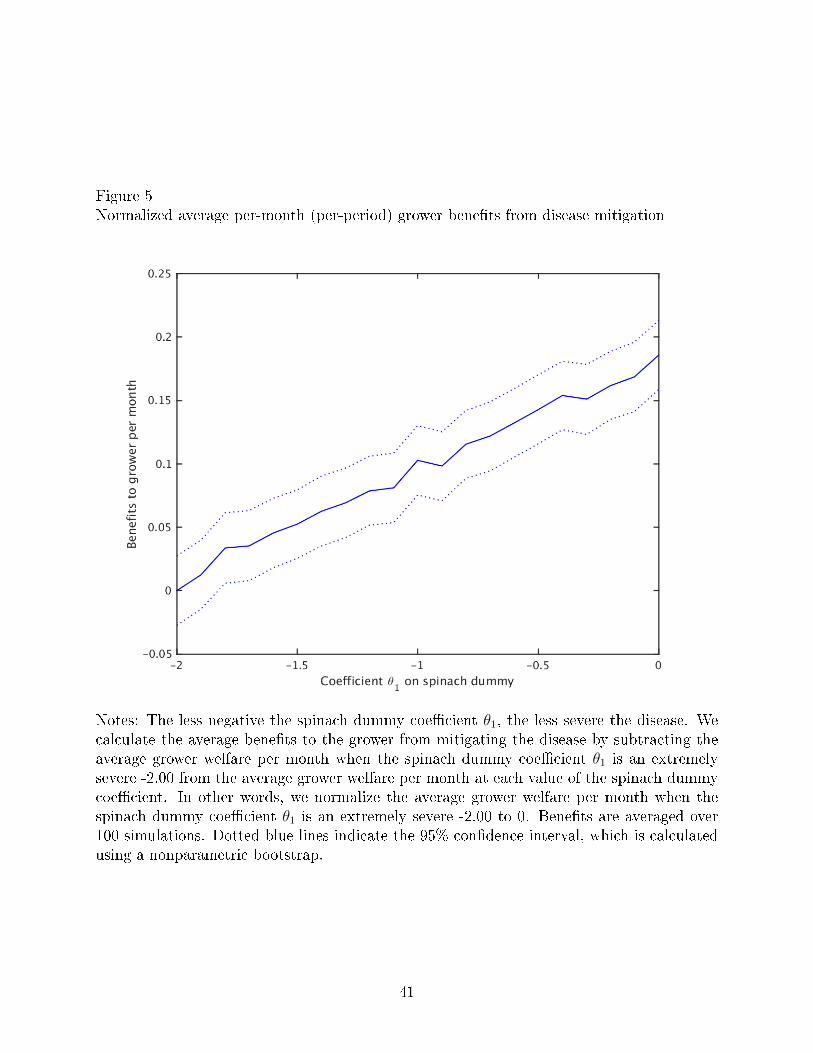
Figure 5Normalized average per-month (per-period) grower bene�ts from disease mitigation

Notes: The less negative the spinach dummy coe�cient θ1, the less severe the disease. Wecalculate the average bene�ts to the grower from mitigating the disease by subtracting theaverage grower welfare per month when the spinach dummy coe�cient θ1 is an extremelysevere -2.00 from the average grower welfare per month at each value of the spinach dummycoe�cient. In other words, we normalize the average grower welfare per month when thespinach dummy coe�cient θ1 is an extremely severe -2.00 to 0. Bene�ts are averaged over100 simulations. Dotted blue lines indicate the 95% con�dence interval, which is calculatedusing a nonparametric bootstrap.

41

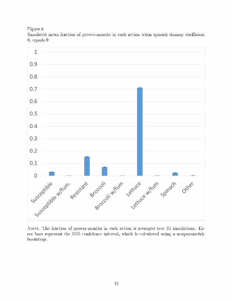
Figure 6Simulated mean fraction of grower-months in each action when spinach dummy coe�cientθ1 equals 0

Notes: The fraction of grower-months in each action is averaged over 25 simulations. Er-ror bars represent the 95% con�dence interval, which is calculated using a nonparametricbootstrap.

42

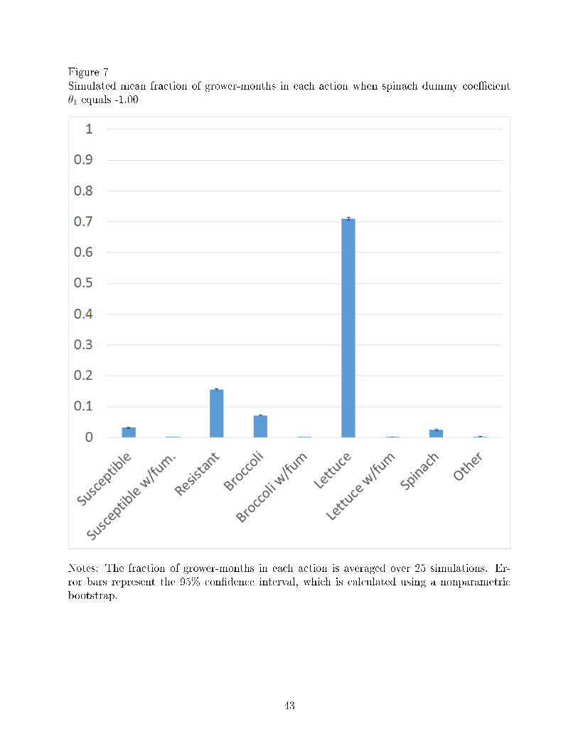
Figure 7Simulated mean fraction of grower-months in each action when spinach dummy coe�cientθ1 equals -1.00

Notes: The fraction of grower-months in each action is averaged over 25 simulations. Er-ror bars represent the 95% con�dence interval, which is calculated using a nonparametricbootstrap.

43

Figure 8Simulated fraction of grower-months in each action type by month of year when spinachdummy coe�cient θ1 equals 0

Susceptible

Sus. w/fum

Resistant

Broccoli

Broccoli w/fum

Lettuce

Lettuce w/fum

Spinach

Other

Month

Notes: The fraction of grower-months in each action by month of year is averaged over 25simulations. Error bars represent the 95% con�dence interval, which is calculated using anonparametric bootstrap.

44

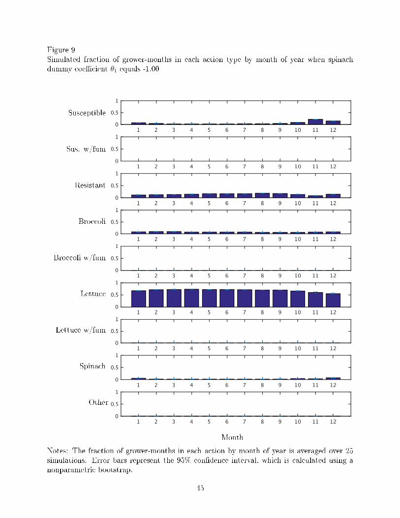
Figure 9Simulated fraction of grower-months in each action type by month of year when spinachdummy coe�cient θ1 equals -1.00

Susceptible

Sus. w/fum

Resistant

Broccoli

Broccoli w/fum

Lettuce

Lettuce w/fum

Spinach

Other

Month

Notes: The fraction of grower-months in each action by month of year is averaged over 25simulations. Error bars represent the 95% con�dence interval, which is calculated using anonparametric bootstrap.

45

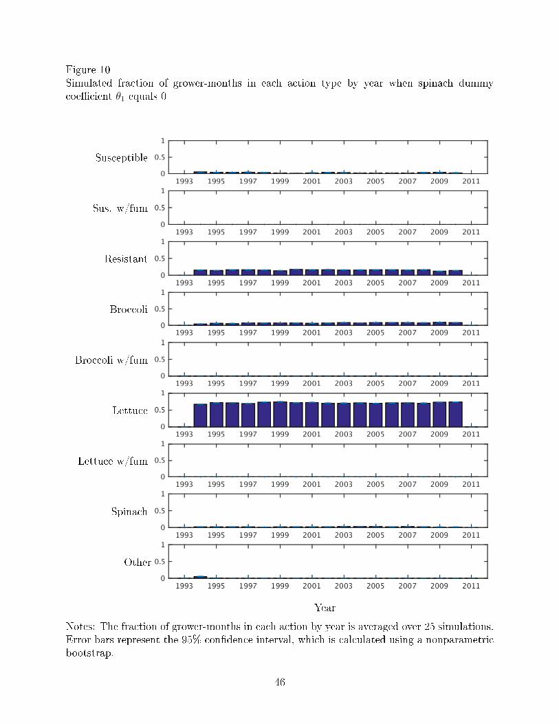
Figure 10Simulated fraction of grower-months in each action type by year when spinach dummycoe�cient θ1 equals 0

Susceptible

Sus. w/fum

Resistant

Broccoli

Broccoli w/fum

Lettuce

Lettuce w/fum

Spinach

Other

Year

Notes: The fraction of grower-months in each action by year is averaged over 25 simulations.Error bars represent the 95% con�dence interval, which is calculated using a nonparametricbootstrap.

46

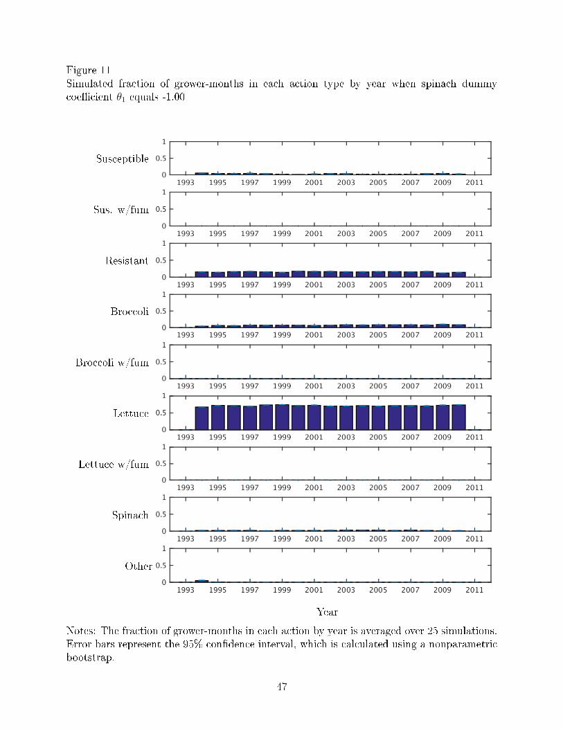
Figure 11Simulated fraction of grower-months in each action type by year when spinach dummycoe�cient θ1 equals -1.00

Susceptible

Sus. w/fum

Resistant

Broccoli

Broccoli w/fum

Lettuce

Lettuce w/fum

Spinach

Other

Year

Notes: The fraction of grower-months in each action by year is averaged over 25 simulations.Error bars represent the 95% con�dence interval, which is calculated using a nonparametricbootstrap.

47

Documents

Crop Disease and Agricultural Productivity