Embed Size (px)
Citation preview
Creating a basic planetary
system in Excel
by
George Lungu
<excelunusual.com>
* For the model presented here it is recommended
that you use Excel 2003 or older. The 2007 will be
either excessively slow.

<excelunusual.com>
We want to create the following model:

<excelunusual.com>
Some basic theory from high school
r
F = u *k*m1*m2 / r^2 – Newton’s universal
attraction formula
F = m*a – Newton’s 2nd law
u=r/|r|
1
2
F
-F

<excelunusual.com>
That was not a very rigorous. Pay attention to few
details:
1.- The forces acting on each body have the same
direction and absolute value but opposite sense
2.- We are talking attraction not repulsion!
3.- The acceleration has the same direction and
sense with the force or gravity.
4. Of course because this problem is in 2-dimens-
sional we need to solve it separately along x and y
axes
<excelunusual.com>
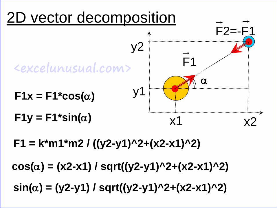
2D vector decomposition
F1x = F1*cos(a)
F1
x2
y1a
F1y = F1*sin(a)
F1 = k*m1*m2 / ((y2-y1)^2+(x2-x1)^2)
x1
y2
F2=-F1
cos(a) = (x2-x1) / sqrt((y2-y1)^2+(x2-x1)^2)
sin(a) = (y2-y1) / sqrt((y2-y1)^2+(x2-x1)^2)

<excelunusual.com>
From Newton’s second law (F = m*a) and the
decomposition formulas we can therefore write the
x and y components of the accelerations of both
bodies as:
a1
x2
y1a
a1x = k*m2* (x2-x1) / ((y2-y1)^2+(x2-x1)^2)^(3/2)
x1
y2a2=-a1
a1y = k*m2* (y2-y1) / (( y2-y1)^2+(x2-x1)^2)^(3/2)
a2x = k*m1* (x1-x2) / ((y2-y1)^2+(x2-x1)^2 )^(3/2)
a2y = k*m1* (y1-y2) / ((y2-y1)^2+(x2-x1)^2 )^(3/2)
a1a1y
a1x

<excelunusual.com>
We also know the definition of acceleration as the
derivative of speed with respect to time:
ax = dvx/dt or ay = dvy/dt
for a very small time increment we can assume that
the acceleration is constant and re-write :
ax_current =(vx_current - vx_previous)/dt
ay_current =(vy_current - vy_previous)/dt
From here we can derive the following:
vx_current = vx_previous + ax_current *dt
vy_current = vy_previous + ay_current *dt <- Very important

<excelunusual.com>Similarily
vx = dx/dt or vy = dy/dt
for a very small time increment we can assume
that the speed is constant and re-write :
vx-current =(xcurrent - xprevious)/dt
vy-current =(ycurrent - yprevious)/dt
From here we can derive the following:
xcurrent = xprevious + vx-current *dt
ycurrent = yprevious + vy-current *dt <- Very important

<excelunusual.com>Outline:
a1x = k*m2* (x2-x1) / ((y2-y1)^2+(x2-x1)^2)^(3/2)
a1y = k*m2* (y2-y1) / ((y2-y1)^2+(x2-x1)^2 )^(3/2)
a1x = k*m1* (x1-x2) / ((y2-y1)^2+(x2-x1)^2 )^(3/2)
a1y = k*m1* (y1-y2) / ((y2-y1)^2+(x2-x1)^2 )^(3/2)
vx_current = vx_previous + ax_current *dt
vy_current = vy_previous + ay_current *dt
The above formulas are all we need to build a
planetary system
xcurrent = xprevious + vx-current *dt
ycurrent = yprevious + vy-current *dt

<excelunusual.com>
So how is the differential equation system
solved?
In the previous page you can see 3
different categories of formulas:
- Acceleration/Force calculations -> yellow
formulas (any time: a=F/m or F=ma)
- Speed calculation -> green formulas
- Coordinate calculations -> blue formulas

<excelunusual.com>
A pure spread sheet type solution
The time in this case time will increase down the
column. Each row will represent a discrete
moment of time.
Advantages of the pure spreadsheet solution:
1. Requires practically no VBA (Visual
Basic for Applications).
2. It is very fast
There are 2 disadvantage of the tabular solution:
1. The number of time steps is limited
2. The files are large

<excelunusual.com>
As we mentioned before, time advances vertically
along the column.
The arrows and their colors relate to each type of
equation:
Forces Speeds Coordinates
Forces Speeds Coordinates
Speeds Coordinatest[0]Initial Conditions
(Constants) ------>
t[1]
t[2]
t[3] etc etc etc
time step - dt

<excelunusual.com>
Some important points:
The forces at time t[n] are calculated from the
coordinates at time t[n-1] -> this is a compromise
which gives decent solutions as long as dt is
small enough (see the yellow formulas)
The speeds are calculated from the previous
speeds (at t[n-1]) and the current accelerations
(see the green formulas)
The coordinates are calculated from the previous
coordinates and the current speeds (see the blue
formulas)
<excelunusual.com>
A sequential type solutionThere is just one row of calculations. A basic VBA
macro will create an infinite loop.
Advantages of the pure spreadsheet solution:
1. It can run forever. It can be stopped and
restarted.
2. The Excel files are small.
The only disadvantage of the sequential solution is
that it is slower than the previous (instantaneous)
version. In our case this does not matter since the
simulation will be display limited ( around 20- 40
frames per second depending on the computer
used and the chart size).

<excelunusual.com>
The macro will copy the speed and coordinate
values from the active row (t[n]) to the following
row.
The arrows and their colors relate to each type of
equation:
Forces Speeds Coordinates
Speeds Coordinatest[n-1] (Constants) ------>
t[n]
time step - dt
The speeds and coordinates at t[n-1] are copied
from the speeds and coordinates at t[n]. Therefore
the formulas are using their old results to calculate
the results in an infinite loop.

So, how is this whole
thing implemented in
Excel?
The following slides
are cookbook-style.
There is no need to
understand the
previous sections .Just
follow the recipe!

<excelunusual.com>
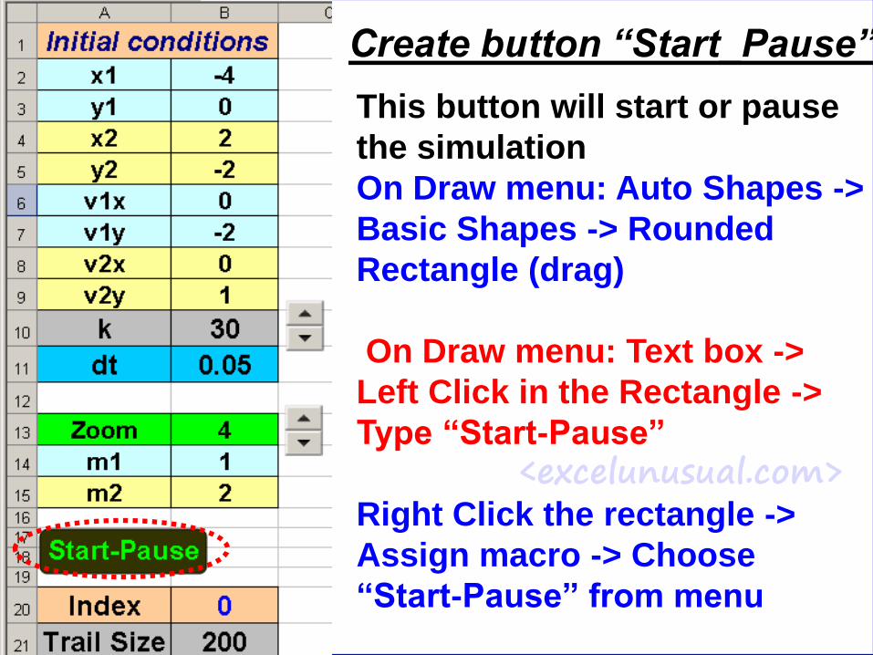
Create the input data area
Cell “A1”: Initial Conditions
Cell “A2”: x1 Cell “A3”: y1
Cell “A4”: x2 Cell “A5”: y2
Cell “A6”: v1x Cell “A7”: v1y
Cell “A8”: v2x Cell “A9”: v2y
Cell “A10”: k
Cell “A11”: dt
Cell “A13”: Zoom
Cell “A14”: m1
Cell “A15”: m2
Cell “A20”: Index
Cell “A21”: Trail Size

<excelunusual.com>
Input data area - figures
I use font size 16 / bold
The only formula is in the
cell “B20”: = L27/B11-1
For the rest of the cells just plug
in those numbers as a starter.

<excelunusual.com>
Create spin button “k”This button will change the
gravitational constant on-the-
fly
View -> Toolbars -> Control
Toolbox -> Spin Button (drag
create)In the control toolbox hit
“Design Mode” then right
click the button and select
“Properties”
Change the following:
(Name): k
Min: 0
Max: 200

<excelunusual.com>
Macro associated to
button “k”
Sub k_Change()
Range("B10") = k.Value
End Sub

<excelunusual.com>
Create spin button “Zoom”
This button will change the
Zoom on-the-fly
View -> Toolbars -> Control
Toolbox -> Spin Button (drag
create)
Right click the button and
select “Properties”
Change the following:
(Name): Zoom
Min: 1
Max: 50
<excelunusual.com>
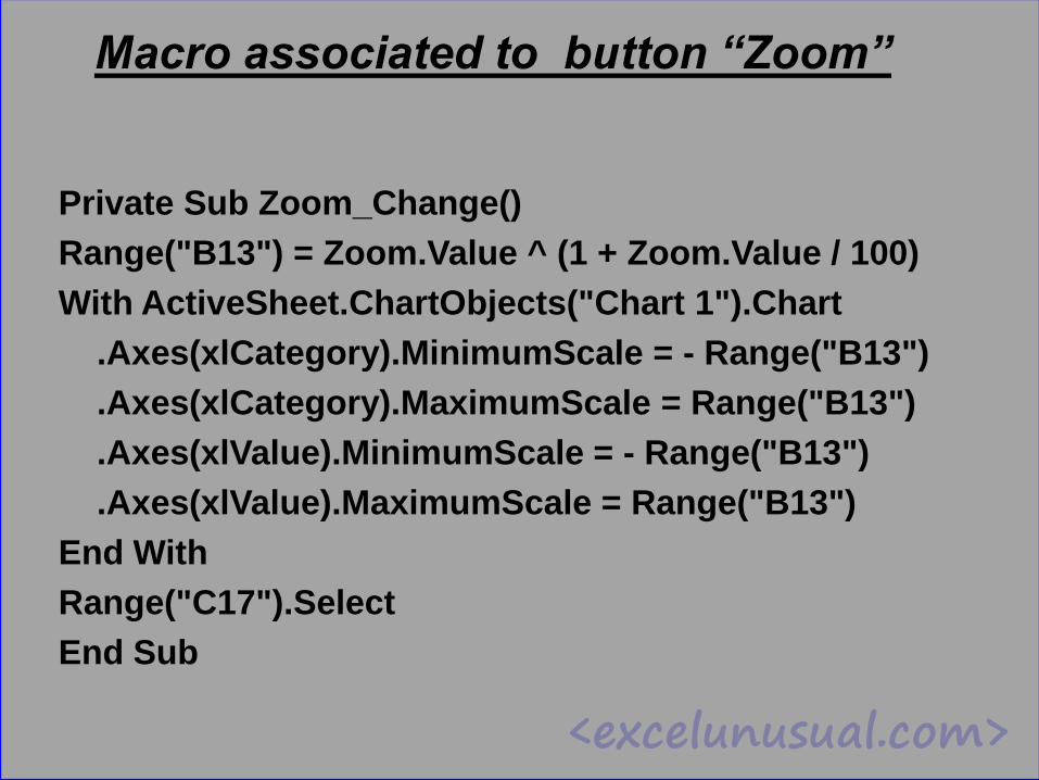
Macro associated to button “Zoom”
Private Sub Zoom_Change()
Range("B13") = Zoom.Value ^ (1 + Zoom.Value / 100)
With ActiveSheet.ChartObjects("Chart 1").Chart
.Axes(xlCategory).MinimumScale = - Range("B13")
.Axes(xlCategory).MaximumScale = Range("B13")
.Axes(xlValue).MinimumScale = - Range("B13")
.Axes(xlValue).MaximumScale = Range("B13")
End With
Range("C17").Select
End Sub

<excelunusual.com>
Create spin button
“Trail_Size”
This button will change the
trail size on-the-fly
View -> Toolbars -> Control
Toolbox -> Spin Button (drag
create)
Right click the button and
select “Properties”
Change the following:
(Name): Trail_Size
Min: 0
Max: 500

<excelunusual.com>
Macro associated to button “Trail_Size”
Private Sub Trail_Size_Change()
Range("B21") = 10 * Trail_Size.Value
Range(Range("D29").Offset(Range("B21"), 0), _
"L5000").ClearContents
End Sub
Just a line break in VBA (the
line was split in 2 by using “ _”
<excelunusual.com>
Create button “Start_Pause”
This button will start or pause
the simulation
On Draw menu: Auto Shapes ->
Basic Shapes -> Rounded
Rectangle (drag)
On Draw menu: Text box ->
Left Click in the Rectangle ->
Type “Start-Pause”
Right Click the rectangle ->
Assign macro -> Choose
“Start-Pause” from menu

<excelunusual.com>
Macro associated to button “Start_Pause”
Public s As Boolean
- - - - - - - - - - - - - - - - - - - - - - - - - - - - - - - - - - - - - - - - - - - - - - - - - -
Sub Start_Pause()
If s = False Then
s = True
Do
DoEvents
If s = False Then Exit Do
Range("D28", Range("L28").Offset(Range("B21"), 0)) = _
Range("D27", Range("L27").Offset(Range("B21"), 0)).Value
Loop
Else
s = False
Exit Sub
End If
End Sub
Just a line break in VBA (the
line was split in 2 by using “ _”

<excelunusual.com>
Observation
Range("D28", Range("L28").Offset(Range("B21"), 0)) = _
Range("D27", Range("L27").Offset(Range("B21"), 0)).Value
Was replaced with:
Range("D28:L28")= Range("D27:L27").Value
The original line of code didn’t give a trail:
Which creates a trail with programmable
length behind each planet

<excelunusual.com>
Create button “Reset”
This button will reset the
simulation
On Draw menu: Auto Shapes ->
Basic Shapes -> Rounded
Rectangle (drag)
On Draw menu: Text box ->
Left Click in the Rectangle ->
Type “Reset”
Right Click the rectangle ->
Assign macro -> Choose
“Reset_” from menu

<excelunusual.com>
Macro associated to button “Reset”
Sub Reset_()
Range("D28:L5000").ClearContents
Range("D28") = Range("B6").Value
Range("E28") = Range("B7").Value
Range("F28") = Range("B8").Value
Range("G28") = Range("B9").Value
Range("H28") = Range("B2").Value
Range("I28") = Range("B3").Value
Range("J28") = Range("B4").Value
Range("K28") = Range("B5").Value
s = False
End Sub
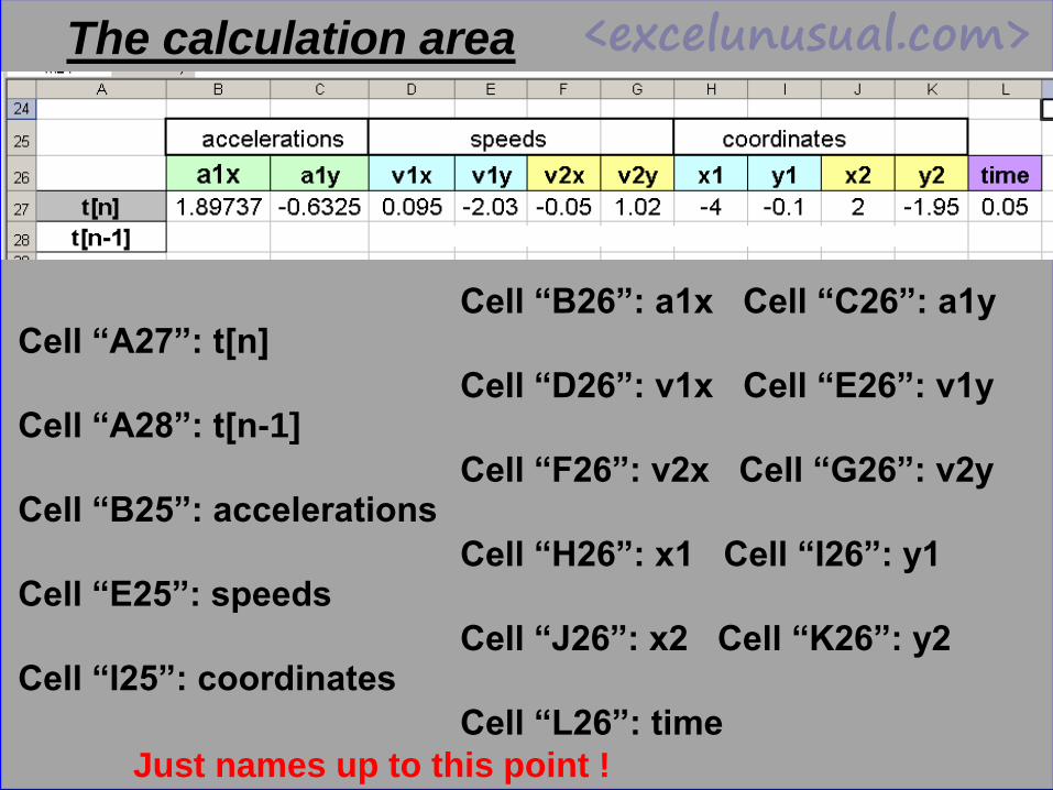
<excelunusual.com>The calculation area
Cell “A27”: t[n]
Cell “A28”: t[n-1]
Cell “B25”: accelerations
Cell “E25”: speeds
Cell “I25”: coordinates
Cell “B26”: a1x Cell “C26”: a1y
Cell “D26”: v1x Cell “E26”: v1y
Cell “F26”: v2x Cell “G26”: v2y
Cell “H26”: x1 Cell “I26”: y1
Cell “J26”: x2 Cell “K26”: y2
Cell “L26”: time
Just names up to this point !

<excelunusual.com>
The calculation area – Active Formulas
Cell “B27”: =B10*B15*B14*(J28-H28)/((J28-H28)^2+(K28-I28)^2)^(3/2)
Cell “C27”: =B10*B15*B14*(K28-I28)/((J28-H28)^2+(K28-I28)^2)^(3/2)
Cell “D27”: =D28+B27*B11/B14
Cell “E27”: =E28+C27*B11/B14
Cell “F27”: =F28-B27*B11/B15
Cell “G27”: =G28-C27*B11/B15

<excelunusual.com>
The calculation area – Active Formulas
Cell “H27”: =H28+D27*B11
Cell “I27”: =I28+E27*B11
Cell “J27”: =J28+F27*B11
Cell “K27”: =K28+G27*B11
Cell “L27”: =L28+B11

<excelunusual.com>
Create the chart
Click on an empty cell -> Insert -> Chart ->
-> XY Scatter -> Finish

<excelunusual.com>
Create the chart - continuation
Delete Legend and Title
Initial conditions
-10
-5
0
5
10
15
20
25
30
35
40
45
0 2 4 6 8 10 12
Initial conditions

<excelunusual.com>
Create the chart - continuation
- Click the white area -> Source
Data Series
- Remove whatever series is
there and Add the following
four series (type them in) ->-10
-5
0
5
10
15
20
25
30
35
40
45
0 2 4 6 8 10 12
- Click on any grid lines and delete them then
change the charting area color to your taste
- Change the font on both axes to 1 (using Format
Axis)

<excelunusual.com>Generate chart data series

Generate chart data series

<excelunusual.com>
Create the chart - continuation
In order to have the Zoom macro work right you
have to name the chart “Chart 1”
You do this by selecting the chart and running
the following macro:
Sub rename()
With ActiveChart
.Parent.Name = "Chart 1"
End With
End Sub
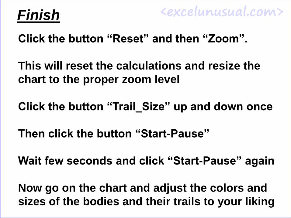
<excelunusual.com>Finish
Click the button “Reset” and then “Zoom”.
This will reset the calculations and resize the
chart to the proper zoom level
Click the button “Trail_Size” up and down once
Then click the button “Start-Pause”
Wait few seconds and click “Start-Pause” again
Now go on the chart and adjust the colors and
sizes of the bodies and their trails to your liking
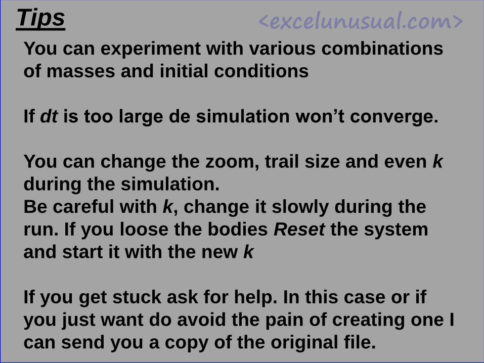
<excelunusual.com>Tips
You can experiment with various combinations
of masses and initial conditions
If dt is too large de simulation won’t converge.
You can change the zoom, trail size and even k
during the simulation.
Be careful with k, change it slowly during the
run. If you loose the bodies Reset the system
and start it with the new k
If you get stuck ask for help. In this case or if
you just want do avoid the pain of creating one I
can send you a copy of the original file.