CPR Data Analysis - pices.int · - 1 - CPR Data analysis The following sections each describe specific investigations with the data that have been undertaken during the project

- 1 -

CPR Data analysis

The following sections each describe specific investigations with the data that have been undertaken during the project. a. Mesozooplankton abundance and biomass An overall description of the abundance of zooplankton available was achieved by summing the abundances of the separately enumerated taxa. The CPR most quantitatively samples the mesozooplankton size range so for this summary the microzooplankton taxa (tintinnids, foraminifera etc.) have been excluded. Mean abundances for 1° latitude bands were calculated for each of the north-south transects (including 1997) and are shown in Figure 1. Abundances are per sample, or approximately per 3m3. The most striking thing is that at no time in 2000 or 2001 were abundances as high as on the 1997 trial transect. There are regional exceptions, most notably the Alaskan shelf where abundances were often higher than in 1997 and also the region around 40-42°N where peaks in abundance were almost always found. This region marks the point at which the ship’s track crosses a high chlorophyll front (evident from SeaWiFs images) and abundances often increased by an order of magnitude from one sample to the next. Comparing the July/August transects of 2000 with the 1997 transect we find that for most of the open ocean region 1997 abundances were 5-10 times higher than in 2000 (mean ratio between 43° and 56°N is 6.2). The Alaskan shelf region, by contrast, was much lower with abundances about one third in 1997 of their 2000 values. The Oregon/Californian coastal region was also higher in 1997, though not so dramatically – the mean ratio being just under 3 times higher in 1997. Comparisons between 1997 and 2001 are restricted by the missing samples from the northern portion of the August transect and the fact that the previous transect was in late June and therefore not at such a comparable time. However, August 2001 abundances were lower again than in 2000.

- 2 -

Although abundance can be considered as a proxy for biomass, changes in species composition can result in changes in biomass irrespective of abundance. A switch from small to large taxa can result in an increase in biomass even if abundances also decline. To examine whether or not the mesozooplankton biomass reflected the same interannual and regional variability we estimated the mesozooplankton biomass of each sample. This was achieved by multiplying the abundance of each taxon by a taxon-specific individual dry weight value and summing the values for each

July/August-97

0 1000 2000

33

36

39

42

45

48

51

54

57

60

Latit

ude

# Organisms

Mar-00

0 500 1000

33

36

39

42

45

48

51

54

57

60

Latit

ude

# Organisms

April/May-00

0 500 1000

33

36

39

42

45

48

51

54

57

60

# Organisms

Jun-00

0 500 1000

33

36

39

42

45

48

51

54

57

60

# Organisms

Jul-00

0 500 1000

33

36

39

42

45

48

51

54

57

60

# Organisms

Aug-00

0 500 1000

33

36

39

42

45

48

51

54

57

60

# Organisms

Apr-01

0 500 1000

33

36

39

42

45

48

51

54

57

60

Latit

ude

# Organisms

May-01

0 500 1000

33

36

39

42

45

48

51

54

57

60

# Organisms

33

36

39

42

45

48

51

54

57

60

-155 -145 -135 -125

June/July-01

0 500 1000

33

36

39

42

45

48

51

54

57

60

# Organisms

Aug-01

0 500 1000

33

36

39

42

45

48

51

54

57

60

# Organisms

Sept-01

0 500 1000

33

36

39

42

45

48

51

54

57

60

# Organisms

Fig. 1. The abundance of mesozooplankton (mean number of organisms per sample) for 1° latitude bands. All transects are plotted on the same scale. There was no sampling in the central section in June 00, the northern section of August 01 and the southern section of September 01.

- 3 -

sample. The dry weight values were derived from actual measurements that have been made of individual organism’s length and dry weight. If measurements were not available for a particular taxon, dry weights were calculated from the published length of the organism and the taxonomically closest organism’s measured length to weight ratio. Mean biomass per region was then calculated but instead of 1° latitude bands the data were divided into hydrographically distinct areas along the transect (Figure 2).

Several features are evident: • Whereas the oceanic abundances were much higher in 1997 than in summer 2000 biomass is

actually not as dramatically different. Biomass was twice as high in the Alaska Gyre region in 1997 than in 2000 and about the same in the more southern oceanic area (numerical abundances were >5 times higher).

• The summer biomass in the Alaska Gyre is actually higher in 2001 than in 1997 or 2000 (although abundances were much lower). The other three areas do have much lower biomass in 2001 than the previous two years, however,

• It appears that the seasonal cycle was advanced in 2001 over 2000, peaks seem to be occurring in May rather than June in the 3 most northern areas. The apparent low biomass and abundances in August 2001 may therefore be because sampling effectively occurred later in the seasonal cycle.

These results show that there is marked interannual variability in either, or both, the absolute amount of plankton present, or the timing at which biomass is at its peak in all regions of the transect. They also suggest that fewer, larger organisms were present in summer 2001, and to some extent 2000, than in 1997.

0

20

40

60

80

100

120

140

160

180

200

July

/Aug

ust

97

Mar

ch 0

0

Apr

il/M

ay00

June

00

July

00

Aug

ust 0

0

Apr

il 01

May

01

June

/Jul

y0

1

Aug

ust 0

1

Sep

tem

ber

01

Mea

n bi

omas

s (m

g dr

y w

t) p

er s

ampl

e (~

3m3) Alaskan Shelf

Alaska GyreOceanic 42-50NOregon/California slope

Fig. 2. Estimated mesozooplankton biomass for each of four regions on each north-south transect. Error bars indicate standard error.

- 4 -

b. Community composition Identification of the plankton on the CPR samples is carried out to the highest practical taxonomic level and is a compromise between taxonomic expertise, achieving detail, and speed of processing. Organisms that are not preserved well by the sampling mechanism, or the formaldehyde preservative, are identified to a high taxonomic level (e.g. Chaetognaths and Larvaceans which are not identified beyond this level). Similarly, organisms that are difficult to identify to species from external morphology alone are identified to the genus level. In practice this means that most calanoid copepods are identified to species (and always to genus) but many groups may not be identified beyond phyla, or class. Responses to environmental change may occur first at the species level, by species replacement for example, and so a lack of specific data may restrict our ability to detect such responses. Two investigations were carried out with the CPR data to determine its feasibility for detecting community composition changes. The first used data from the transects across the Pacific, from Vancouver, Canada to Kamchatka (2000) and Japan (2001) to examine geographical changes in community composition. The second used calanoid copepod data only from the Alaska to California transects to examine interannual variability in copepod community composition.

i. Zooplankton communities across the north Pacific

The east to west CPR transect can be subdivided into geographic regions that might be expected to have different combinations of planktonic species, owing to proximity to the coast or physical environment for example. Multidimensional scaling (MDS) is an analysis tool that compares the number and type of individuals in a sample and constructs a two dimensional representation of the similarity of the samples. Samples that plot closest together are therefore most similar in their species composition. In the following MDS analyses only samples collected during the day were used since diel vertical migration results in some species being present at night only. At these high latitudes in June only a few night-time samples are collected so that most of the samples were included in the analysis. Ambiguous taxa (such as ‘copepod nauplii’ or ‘unidentified Neocalanus’) which could belong to more than one of the more specific taxon categories were removed from the analysis. Abundances were transformed (log(x+1)) prior to analysis to increase the contribution of rare species. All unambiguous zooplankton taxa were included, even those that are small and probably undersampled by the CPR because we assume that the CPR catches a consistent portion of these groups. Each year was treated separately initially, and then a combined analysis was carried out. The plots in Figure 4 have been coloured according to the geographic region the samples were collected from to clarify the spatial patterns. Stress values for the analyses were close to the maximum for which a 2 dimensional plot is appropriate (~0.2 in each case). Stress is a measure of the distortion between the actual numerical similarity values and the corresponding distances in the resulting plot. Nonetheless, geographical clustering of samples is clear and particularly in 2000 there is an east to west gradient evident in the plot (from right to left). The extreme west samples (collected off the Kuriles Islands in 2001 only) form a cluster within the western Pacific samples. The Bering Sea samples are indistinguishable from the western Pacific samples in 2000 but there is some separation in 2001. In fact, there are two distinct groupings of Bering Sea samples in 2001 but there is no geographic correspondence. Samples from the Gulf of Alaska show the greatest variability. Much, but not all,

- 5 -

of this can be described by subdividing the Gulf into east, west and central (as shown). However, the western GoA samples in 2001 were extremely variable.

The analysis was repeated with 2000 and 2001 samples combined. The resulting plot is not shown but the samples remained clustered according to geographic region, rather than year. This implies that the regional differences in community composition were stronger than interannual differences in any one region. Examination of the taxa recorded also verifies that the same groups were found in both years. The most frequently occurring taxa in each region are often the same as in other regions (Appendix) and it is changes in the relative rankings of these common groups that cause much of the differentiation between areas. However, there are also less common taxa which are restricted to some areas only (lower panel, Appendix). Transformation of the data gives some weight to these rarer groups in the analysis.

ii. Northern versus southern copepod species There is a growing consensus that the El Niño of 1997/98 marked the transition to a new ‘regime’ in the north Pacific, beginning in 1999 (Schwing and Moore, 2000). Studies of zooplankton collected along the Newport Line (Newport, Oregon) have identified that certain copepod species can be designated as boreal or subtropical, and that their abundance off Newport in a given year is likely related to climatic conditions. An increase in biomass occurred after 1998 together with a switch to colder regime species (Peterson et al., 2001). Mackas et al. (2001) report that between

Fig 3. MDS analyses of the zooplank ton on the east to west transect. Samples have been coloured according to location (bottom panel). The two transects are also shown, 2000 being shorter and more northerly than 2001,

2000

Coastal British ColumbiaEastern GoACentral GoAWestern GoAAleutian ShelfBering SeaW. Open PacificKuriles Islands

2001

- 6 -

1990 and 1998 the zooplankton community of the British Columbia continental shelf edge consisted of southerly copepod and chaetognath species endemic to the California Current system with a corresponding decline in species endemic to the Northeast Pacific continental margin. This observed pattern changed abruptly in 1999. The CPR data contains species level information for most calanoid copopods. To detect a regime shift normally requires multiple years of data before and after the shift. However, a comparison of the 1997 copepod data (warm regime) with the 2000/2001 copepod data (cool regime) could provide an indication of the strengths of CPR data in detecting climate related community composition changes. Abundance of each copepod species (or genus if the highest level) was correlated with latitude for all samples collected on the Alaska to California transect, except those samples collected over the continental shelf (north of 59°N and south of 40°N). This eliminated the more neritic species that occurred at both extremes of the transect and which may have confused the analysis. Species that correlated positively with latitude were termed ‘northern species’ and those that correlated negatively were termed ‘southern species’ (Table 1). Table 1. Northern species are those whose abundance correlated positively with latitude, southern species correlated negatively between 40° and 59°N.

Northern Species Southern Species Acartia longiremis Acartia danae Acartia spp. Calanus pacificus Calanus marshallae Candacia armata Candacia colombiae Candacia bipinnata Centropages bradyi Candacia ethiopica Eucalanus attenuatus Clausocalanus spp Eucalanus bungii Corycaeus spp. (note, cyclopoid not calanoid) Eucalanus elongatus Euchirella pseudopulchra Heterorhabdus tanneri Euchirella rostrata Neocalanus cristatus Mecynocera clausi Neocalanus plumchrus/flemingeri Mesocalanus tenuicornis Oncaea spp. Metridia pacifica Paraeuchaeta elongata Nannocalanus minor Pseudocalanus spp. Pleuromamma abdominalis Sapphirina spp. Scolecithrix spp. Undeuchaeta bispinosa Undeuchaeta major Undeuchaeta plumosa

Southern and northern indices were calculated for each sample by summing the abundances of the respective species (Figure 4). Keeping in mind that there is just a single transect from the ‘warm regime’ and any conclusions drawn from this analysis must be somewhat speculative,

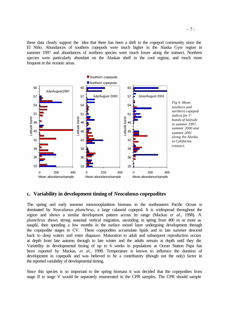
- 7 -

these data clearly support the idea that there has been a shift in the copepod community since the El Niño. Abundances of southern copepods were much higher in the Alaska Gyre region in summer 1997 and abundances of northern species were much lower along the transect. Northern species were particularly abundant on the Alaskan shelf in the cool regime, and much more frequent in the oceanic areas.

c. Variability in development timing of Neocalanus copepodites The spring and early summer mesozooplankton biomass in the northeastern Pacific Ocean is dominated by Neocalanus plumchrus, a large calanoid copepod. It is widespread throughout the region and shows a similar development pattern across its range (Mackas et al., 1998). N. plumchrus shows strong seasonal vertical migration, ascending in spring from 400 m or more as nauplii, then spending a few months in the surface mixed layer undergoing development through the copepodite stages to CV. These copepodites accumulate lipids and in late summer descend back to deep waters and enter diapause. Maturation to adult and subsequent reproduction occurs at depth from late autumn through to late winter and the adults remain at depth until they die. Variability in developmental timing of up to 6 weeks in populations at Ocean Station Papa has been reported by Mackas, et al., 1998. Temperature is known to influence the duration of development in copepods and was believed to be a contributory (though not the only) factor in the reported variability of developmental timing. Since this species is so important to the spring biomass it was decided that the copepodites from stage II to stage V would be separately enumerated in the CPR samples. The CPR should sample

Fig 4. Mean southern and northern copepod indices for 1° bands of latitude in summer 1997, summer 2000 and summer 2001 along the Alaska to California transect.

0 200 400

33

36

39

42

45

48

51

54

57

60

Latit

ude

band

Mean abundance/sample

July/August1997

0 200 400

33

36

39

42

45

48

51

54

57

60

Latit

ude

band


Southern copepods

Northern copepods

July/August 2000

0 200 400

33

36

39

42

45

48

51

54

57

60

Latit

ude

band


June/August 2001

- 8 -

the surface populations of the copepodites of N. plumchrus quite well, owing to their size and the fact that their diel vetical migration is negligible. However, it was found difficult to separate N. plumchrus from its congener N. flemingeri in routine processing and so although N. plumchrus probably dominates, the two have not been separated. It became apparent during the processing of the 2000 samples that the younger copepodite stages were present later in the season in the more northern areas and were rare, or absent, in the most southern samples after the first transect in March 2000. Faster development and maturation is expected in warmer temperatures, and so the data were examined to determine this variability along the transect and whether or not temperature changes were sufficient to explain it. Full details of this study are given in Batten et al (in press) and will be summarised here. The transect was divided into four approximately equal regions according to latitude, and the mean stage composition of the copepodites in each region calculated. Previous studies (Mackas et al, 1998) had suggested that the maximum surface biomass of N. plumchrus occurred when 50% of the copepodites had reached stage V. It was possible to estimate the date at which this occurred by interpolation (Fig 5). Using this criterion we have estimated that the difference between maximum biomass in the southern and northern areas was about 39 days. Using published relationships between body size, temperature and development duration (Hirst and Kiørboe, 2002) we predicted that at the measured surface water temperatures duration of development would be about 3 weeks shorter in the most southern area compared to the most northern area. Other factors may play a role, including the speed of lipid accumulation. Additionally, the transects were sampled every 4-5 weeks and so a linear interpolation between sampling dates may be too simplistic and not necessarily accurate enough. This exercise was repeated with the 2001 data. Unfortunately the first sampling occurred in late April, rather than March as in the previous year, and it was discovered that in all but the most northern area the majority of the copepodites were already at stage V. It was only possible to estimate the time of peak biomass for the area >55°N, where less than 50% were at stage V at the

0%

25%

50%

75%

100%

Stage VStage IVStage IIIStage II

> 55°N

0%

25%

50%

75%

100%

50°-55°N

0%

25%

50%

75%

100%

45°-50°N

0%

25%

50%

75%

100%

22/0

3

05/0

4

19/0

4

03/0

5

17/0

5

31/0

5

14/0

6

28/0

6

12/0

7

Date

41°-45°N

Fig. 5. The proportion of the N. plumchrus/flemingeri population made up of each copepodite stage in 2000, for 4 divisions of the transect. The lines mark the point at which 50% of the population is at stage V in each division.

- 9 -

first sampling, and this date was predicted as the 2nd May. In 2000, for the same, area, this date was predicted as 27th May. Even allowing for inaccuracies of the interpolation method the stage composition data alone show that the development was much advanced in 2001, and this too was considered a ‘cold’ year. d. Large and meso-scale patchiness

i. Decorrelation length scales Large scale patchiness (on the order of 10s to 100s of kms) needs to be considered as a factor that may contribute to the observed variability in the plankton data. The maximum resolution possible from CPR data is 18.5 km, however, to maximise coverage with the resources available we planned for a resolution of 74 km for this project (every fourth sample being processed). Since one objective was to examine the sampling strategy and recommend modifications for the future, if necessary, we carried out an analysis of the CPR data to examine the size of observed patches of particular organisms. Sequentially lagging an abundance series and calculating its autocorrelation enables the decorrelation length scale to be determined, i.e. the point (distance) at which the series no longer significantly correlates with itself. At this point samples are statistically independent. One transect was selected for ‘over-sampling’. The April 2000 transect was sampled as normal but every sample collected was processed instead of every fourth. Samples were therefore continuous with the midpoint of consecutive samples being 18.5 km apart. The entire transect from Alaska to California takes about 5 or 6 days to cover. For this analysis we have ignored samples collected on the shelf at the extremes of the transect as the shelf break causes an abrupt change in the number and/or type of organisms present. Similarly, surface species composition often changes at twilight and dawn because of diel vertical migration by some species. More day-time samples were collected than night-time and so the analysis only used samples collected after dawn but before twilight. The oceanic section of the transect was sampled over 4 days and we have considered each day of sampling as a replicate. 15 to 18 consecutive samples were collected and processed for each of the four replicate days. For the most commonly occurring taxonomic entities on each day (ranked according to frequency of occurrence) autocorrelations of abundance were carried out by lagging the series of sequential abundances by 1 sample, 2 samples, 3 samples etc until only the first and last samples were paired. With each additional lag the number of paired samples to correlate decreases and so the threshold correlation coefficient for a significant correlation increases. Figure 6 shows the resulting correlations and the 95% confidence interval for each analysis. Only those correlation coefficients outside the confidence limits are considered statistically significant. The pattern shown for the Para-pseudocalanus group, particularly on day 1 and 2 suggests that some patches do occur for this group. Significant positive correlations are found with low sample distances, up to about 20-30 km and then significant negative correlations occur at large distances. However, for most of the groups there are sporadic significant correlations but no clear pattern. This suggests that patches are occurring either at scales smaller than about 1 CPR sample (i.e. less than 20 km) or larger than 15-18 samples (larger than about 300 km). This supports the belief that the CPR sampling resolution is adequate for a synoptic survey of the entire north

- 10 -

Pacific. An individual sample will pass through small patches of plankton and so provide an ‘average’ of the small-scale patchiness. Samples that are spaced well apart, such as every 74 km, are likely to be representative and not likely to be within or outside of a patch.

Fig. 6. Autocorrelations of abundances of common taxa for each of four days in April 2000 along the Alaska to California transect. Only day time samples were used. Red dashed lines show 95% confidence limits. Blanks occur where insufficient numbers were present for analysis.

- 11 -

ii. Coastal plankton associated with eddies

Attention was focussed in 2000 on the large anticyclonic eddies formed at the eastern continental margin of the north Pacific, in the region south of the Queen Charlotte Islands (also known as the Haida eddy) and off Sitka, southeast Alaska. These eddies, which have a diameter of up to 200 km or more, form during the winter months and in late winter spin off the shelf and move out into the open ocean. Dedicated research cruises sampling the eddies had revealed elevated levels of entrained near-shore and slope zooplankton species that persisted within the Haida 2000 eddy for over a year (Mackas and Galbraith, submitted). The Alaska to California CPR transects passed through, or very close to, these eddies and raised the possibility of establishing whether or not the sampling resolution was capable of detecting such mesoscale features, and also establishing the possible persistence of shelf species in the open ocean. Sea surface altimetry plots (TOPEX & ERS2, see www-ccar.colorado.edu/~realtime/global-real-time_ssh/) were used to determine the location and midpoint of each eddy at the time of each sampled transect. Distance from the midpoint of each sample to the midpoint of the closest eddy centre was calculated and the abundance of each taxon against distance examined. The relationship between abundance and distance from the eddy revealed three classes of plankton that appeared to be associated with eddies; 1. Diatoms: Thalassiosira spp., Chaetoceros spp. (Hyalochaete forms), Coscinodiscus spp. and Cylindrotheca closterium. 2. Zooplankton species of shelf origin: Acartia longiremis and Calanus marshallae 3. Zooplankton taxa that are also common in the open ocean: Limacina helicina, Chaetognaths, copepod nauplii, Clione limacina, Neocalanus plumchrus. 1. Diatoms Of the four groups that show an association, Thalassiosira and Chaetoceros are very common across the northeast Pacific. The species of the genus Thalassiosira and the Hyalochaete subgenus of Chaetoceros are principally neritic (Cupp, 1943) and both groups have highest abundances in coastal CPR samples (Fig 7). The higher oceanic abundances associated with the eddies reflects the coastal origin of the water. The genus Coscinodiscus has not been recorded on many coastal CPR samples, and its highest abundances are associated with the Sitka eddy only. Most species of this genus are oceanic although some are neritic. Without further identification it is not possible to determine whether the increased abundances near the Sitka eddy are the result of entrained neritic species or an enhancement of oceanic abundances. Cylindrotheca closterium was found relatively rarely with highest abundances near the coast. This diatom is a littoral species, although frequently found in the plankton (Cupp, 1943), and so its oceanic occurrences in the region of the eddies again reflect the coastal origins of the water. 2. Shelf zooplankton species Two species of calanoid copepod, Calanus marshallae and Acartia longiremis, are frequently found on CPR samples wherever the trackline approaches or crosses the continental slope (the Alaskan shelf south of Prince William Sound, near the Oregon/Californian shelf, near Vancouver Island, British Columbia around the Aleutian Islands and in the southern Bering Sea), but only rarely in the open ocean (Fig 8).Neither species has occurred on samples from the western Gulf

- 12 -

of Alaska. C. marshallae and A. longiremis were also identified by Mackas and Galbraith (submitted) as continental shelf species occurring in the Haida eddy, although C. marshallae relatively rarely. It occurred on the oceanic CPR samples in 2000 only 5 times. However all of these samples were within 200 kms of the centre of the Haida 2000 eddy, hence its inclusion here as a species indicative of coastal water. Further shelf species may also have a signal in CPR samples but many taxa, except most calanoid copepods, are not identified to species level in routine CPR processing. Mackas and Galbraith (submitted) identify Pseudocalanus mimus as a shelf species associated with the Haida 2000 eddy, however, in CPR processing the highest taxonomic resolution is to the genus Pseudocalanus. Oceanic species of this genus exist so that an association with the eddy in CPR samples is not evident.

Calanus marshallaeAcartia longiremis

Thalassiosira spp. Chaetoceros spp. Hyalochaete form

Coscinodiscus spp. Cylindrotheca closterium

Fig. 7. The occurrence of ‘shelf taxa’ on CPR samples in the northeast Pacific in 2000 and early 2001. The 1000m isobath is also shown. For the zooplankton (top) the symbols represent abundance as follows: A. longiremis - the largest symbol indicates abundances of ~600 m-3 and the smallest symbol ~15 m-3 . For C. marshallae the largest symbol indicates abundances of ~12 individuals m-3 and the smallest symbol ~1 m-3. For the phytoplankton taxa (below) the symbols are scaled to the number of microscope fields of view per sample that the diatoms were seen in, from 1 to 20 (max).

- 13 -

3. Oceanic species Several species which commonly occur throughout the northeast Pacific showed an association with the eddy. Neocalanus plumchrus copepodites III and IV are only present in surface waters for a few weeks in spring. During March especially higher abundances were clearly associated with the eddies. By July 2000 only a small number of individuals (copepodites IV and V) were still in surface waters (Batten, et al., in press) and by August all had descended to diapause. This restricts the samples where associations might be seen to the spring and early summer transects. Most samples close to the eddies had chaetognaths and the pteropod Limacina helicina present. Although equally high numbers of these groups occurred well away from the eddy, counts of zero were also more frequent away from the eddy. The pteropod Clione limacina, which feeds almost exclusively on L. helicina, was infrequently caught but predominantly on samples close to the eddy. The copepod nauplii category may have been more revealing if the parent species (and thus their origins) were known, however it is likely that both shelf and oceanic species contributed to the high abundances near the eddies. L. helicina and N. plumchrus were also reported as having high abundances in samples from the Haida eddy by Mackas and Galbraith (submitted). All of the coastal/shelf species associated with the eddy have generation times shorter than half of the sampling season in 2000, therefore, any individuals recorded on the eddy samples in July or August were most probably offspring of the original advected organisms. Diatoms have generation times of ~1 day so that any occurrences after the eddy left the shelf in March indicate a reproducing population. Thalassiosira and Chaetoceros were both most abundant in the oceanic samples in March and April but were still being recorded in August. Coscinodiscus was found only sporadically after June and C. closterium was found in March and April but then not again until August. The August abundances are intriguing, given that this benthic species should not be reproducing in the plankton, however, there were several records of it in August so that it is unlikely to be an error. A. longiremis has a generation time of about 1 month over the northern Oregon shelf (Peterson et al., 1979) which is likely to be similar to the rate off the coast of British Columbia. Highest oceanic abundances were recorded in June but there were no more occurrences around the Haida eddy in subsequent months. It was also recorded around the Sitka eddy in August. C. marshallae has a development time of ~36 days at 15°C and ~64 days at 10°C (Peterson, 1979). Temperatures at 52°N, 135°W (the vicinity of the Haida eddy) were 7°C on the March transect, 10.5°C on the June transect and 13°C on the July transect (Batten et al., in press) suggesting a generation time of close to 60 days. Although only a few eddy samples contained C. marshallae it was present in all months except July. August occurrences must have been from at least the second generation in the eddy. Maintenance of the population in the eddy would enhance the spread of shelf species through the open ocean by increasing both the time available for distribution and the number of source organisms. The Haida 2001 eddy was much weaker than the Haida 2000 and it might be predicted that oceanic occurrences of coastal taxa would be less frequent in 2001. With the exception of C. marshallae, which had low occurrences in any case, all of the associated shelf taxa showed a marked decline in oceanic occurrence in 2001. The decline in oceanic occurrence of shelf taxa between 2000 and 2001 was significant (p<0.05, paired 2 sample t-test). The 6 oceanic taxa associated with the eddy in 2000 showed no significant change in frequency of occurrence (p>0.05, paired 2 sample t-test).

- 14 -

This study demonstrates that the CPR sampling resolution is sufficient to identify the influence of mesoscale features on plankton species distributions. Furthermore, both the temporal and spatial scale of sampling has enabled us to comment on the extent and the variability of this influence. Summary The principal objective of the project has been achieved, namely that a plankton monitoring program has been initiated and is returning valuable baseline data. We have given examples of how the data have been used to describe seasonal cycles of mesozooplankton abundance and biomass, spatial variability in community composition and also distributions of key species. Assessments of interannual variability, and likely influences of climate fluctuations, can only be preliminary with data from just three years currently available, however, its clear from the results described here that the program has the potential to address this aspect as more data are acquired. We have described changes in the quantity of zooplankton and also the type of species present that are consistent with the change from warm to cool conditions at the end of the 1990s. The analyses suggest that spring 2001 occurred earlier in the year than in 2000; the oceanic biomass cycle peaked about one month earlier and maturation of Neocalanus copepodites also occurred earlier. It is highly unlikely that these two years represent the maximum variability in seasonality. In addition, the interannual variability in overall abundance and biomass seems to be large, factors of at least 2 and perhaps as much as 5 times, and so one conclusion already suggested is that the plankton of the northeast Pacific is highly variable on large scales. This variation may provide part of the mechanistic linkage between climate change and productivity of fish populations. One limitation of the CPR data is that the plankton are collected from a fixed depth of about 7m, which is shallower than where the majority of the zooplankton biomass is found, and too shallow for some species to be sampled at all. As with all plankton sampling devices, only a fraction of the plankton community is sampled, mostly because the aperture of the device and the filtering mesh size restrict the upper and lower size classes that can be sampled. We have to assume that this fraction is consistent, but it means that we can only comment on changes in the plankton that are likely to be sampled by the CPR. Additionally, the identification of some organisms into quite coarse taxonomic categories limits the species level changes that can be described. Since all samples are archived, however, it would be possible to re-examine the samples to identify key organisms further if such an exercise were required, and provided that the necessary features are distinguishable given the CPR sampling characteristics. Our analyses of the sampling resolution suggest that it is adequate to describe mesoscale and larger features and is unlikely to be significantly biased. The approximately five weekly temporal spacing also appears to be adequate to determine seasonal cycles and seasonal succession although the detection of fluctuations at less than a monthly resolution will not be realistic. There is no evidence so far to suggest that the sampling strategy should be modified. References Batten, S.D., Welch, D.W., and Jonas, T. (In press). Latitudinal differences in the duration of development of Neocalanus plumchrus copepodites. Fisheries Oceanography

- 15 -

Cupp, E. (1943). Marine plankton diatoms of the west coast of North America. Bull. Scripps Instn. Oceanogr., 5. Hirst AG, Kiørboe T (2002). Mortality of marine planktonic copepods: global rates and patterns Marine Ecology Progress Series 230:195-209 Mackas, D.L. & Galbraith, M.D. (submitted). Zooplankton distribution and dynamics in a north Pacific eddy of coastal origin: I. Transport and loss of continental margin species. Mackas, D.L., Goldblatt, R., and Lewis, A.G. (1998) Interdecadal variation in development timing of Neocalanus plumchrus populations at Ocean Station P in the subarctic North Pacific. Can. J. Fish. Aquat. Sci. 55: 1878-1893. Mackas, D.L., Thomson, R.E. and Galbraith, R.E. (2001). Changes in the zooplankton community of the British Columbia continental margin, 1985-1999, and their covariation with oceanographic conditions. Canadian Journal of Fisheries and Aquatic Sciences, 58, 685-702. Peterson, W.T. (1979). Life history and ecology of Calanus marshallae (Frost) in the Oregon upwelling zone. PhD thesis, Oregon State University, pp. 200. Peterson, W., Keister, J.E. and Pinnix, W.D. (2001). The 1998/99 Regime Shift in the northern California Current: What are the copepods telling us? Presentation at PICES 10th Annual Meeting, Victoria, British Columbia, Canada, October 2001. Schwing, F. and Moore, C. (2000). A year without summer for California, or a harbinger of a climate shift. EOS, Transactions, American Geophysical Union 81: 301,304-305

- 16 - 2000 2001 2000 2001 2000 2001 2000 2001 2000 2001 2000 2001 2000 2001 2001

British Columbia shelf

Eastern Gulf of Alaska

Central Gulf of Alaska

Western Gulf of Alaska

Aleutian Shelf Bering Sea Western Open Pacific

Kuriles Islands

Common Taxa Acartia longiremis

Acartia spp. Para-pseudocalanus spp.

N.plumchrus/flemingeri V

Foraminifera

Foraminifera

Oithona spp.

Foraminifera

Para-pseudocalanus spp.


Oithona spp.

Foraminifera

Oithona spp.

Oithona spp.

Oithona spp.


Acartia longiremis

Limacina sp.


Limacina sp.

Foraminifera

Limacina sp.

Acartia longiremis

Acartia longiremis






Parafavella gigantea

Oithona spp.


Oithona spp.

Limacina sp.



Oithona spp.

Limacina sp.

Limacina sp.


Oithona spp.

Calanus spp I-IV

Foraminifera

Calanus spp I-IV


Acartia longiremis


Oithona spp.

Oithona spp.

Pseudocalanus Adult

Larvacea Acartia spp. Acartia spp. Foraminifera

Limacina sp.

Foraminifera

Calanus spp I-IV

Foraminifera

Larvacea Euphausiacea calyptopis

Foraminifera

Acartia longiremis

Pseudocalanus Adult


Ptychocylis spp.

N.cristatus V_VI

Oithona spp.

Oithona spp.

Chaetognatha juv.

Calanus spp I-IV


Limacina sp.

N.plumchrus/flemingeri II

Euphausiacea calyptopis

Pseudocalanus Adult

Oithona spp.

Acartia spp. Ptychocylis spp.

Chaetognatha juv.

Calanus spp I-IV


Foraminifera

Foraminifera

Calanus spp I-IV


N.cristatus V_VI

Eucalanus bungii

Ptychocylis spp.

Calanus marshallae V_VI

Limacina sp.

Euphausiacea

Acartia danae


Larvacea Acartia longiremis

Chaetognatha juv.

Pseudocalanus Adult

Pseudocalanus Adult

Pseudocalanus Adult

Ptychocylis spp.

Limacina sp.


Limacina sp.

Decapoda larvae

Centropages abdominalis

Pseudocalanus Adult

N.cristatus V_VI

Chaetognatha adult

Pseudocalanus Adult

Parafavella gigantea

Hyperiidea Euphausiacea Hyperiidea Eucalanus bungii

Hyperiidea Acartia spp. Chaetognatha juv.

Epilabidocera amphrites


Limacina sp.

Hyperiidea Euphausiacea

N.cristatus V_VI

Hyperiidea Fish larvae N.plumchrus/flemingeri V


N.cristatus V_VI


Chaetognatha juv.


Cirripede larva

Tomopteris N.plumchrus/flemingeri IV

Echinoderm larvae

Euphausiacea

Calanus pacificus V_VI

Chaetognatha adult

N.plumchrus IV

Clione limacina

N.cristatus V_VI

N.cristatus V_VI

Acartia spp. Acartia spp. Pseudocalanus Adult

Chaetognatha juv.

Larvacea

Rarer taxa

Centropages abdominalis

* * *

Calanus marshallae * * * * * * Echinoderm larvae * * * * Cyphonautes larvae * * * Ostracoda * * * * Scolecithricella spp. * Eucalanus bungii * * * * * *

Appendix. East-west transect. East-west transect. Ten most numerically abundant taxa in each geographic region, each year, ranked in descending order. Lower panel lists selected less common taxa and the regions in which they were found (see Section b.i.).

Documents

CPR Data Analysis - pices.int · - 1 - CPR Data analysis The following sections each describe specific investigations with the data that have been undertaken during the project