Embed Size (px)
Citation preview

• Cost: $200,000 + $10,000 shipping + $30,000 installation.
• Depreciable cost $240,000.
• Economic life = 4 years.
• Salvage value = $25,000.
• MACRS 3-year class.
Proposed Project
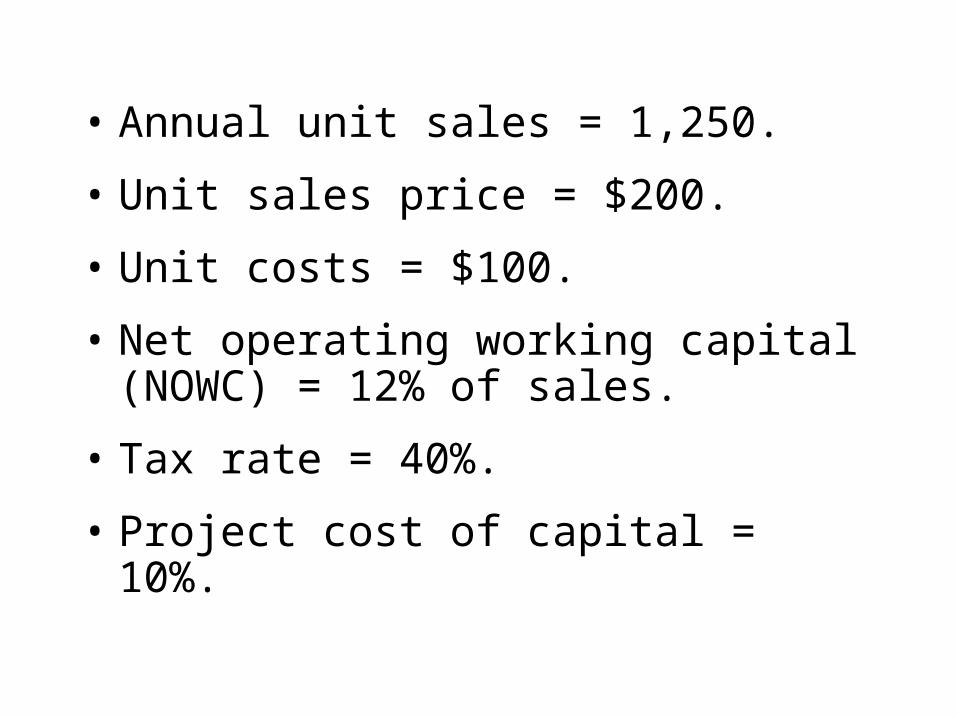
• Annual unit sales = 1,250.
• Unit sales price = $200.
• Unit costs = $100.
• Net operating working capital (NOWC) = 12% of sales.
• Tax rate = 40%.
• Project cost of capital = 10%.

Incremental Cash Flow for a Project
• Project’s incremental cash flow is:
– Corporate cash flow with the project
Minus – Corporate cash flow without the project.

• NO. We discount project cash flows with a cost of capital that is the rate of return required by all investors (not just debtholders or stockholders), and so we should discount the total amount of cash flow available to all investors.
• They are part of the costs of capital. If we subtracted them from cash flows, we would be double counting capital costs.
Should you subtract interest expense or dividends when calculating CF?

• NO. This is a sunk cost. Focus on incremental investment and operating cash flows.
Suppose $100,000 had been spent last year to improve the production line
site. Should this cost be included in the analysis?

• Yes. Accepting the project means we will not receive the $25,000. This is an opportunity cost and it should be charged to the project.
• A.T. opportunity cost = $25,000 (1 - T) = $15,000 annual cost.
Suppose the plant space could be leased out for $25,000 a year. Would
this affect the analysis?

• Yes. The effects on the other projects’ CFs are “externalities”.
• Net CF loss per year on other lines would be a cost to this project.
• Externalities will be positive if new projects are complements to existing assets, negative if substitutes.
If the new product line would decrease sales of the firm’s other products by
$50,000 per year, would this affect the analysis?
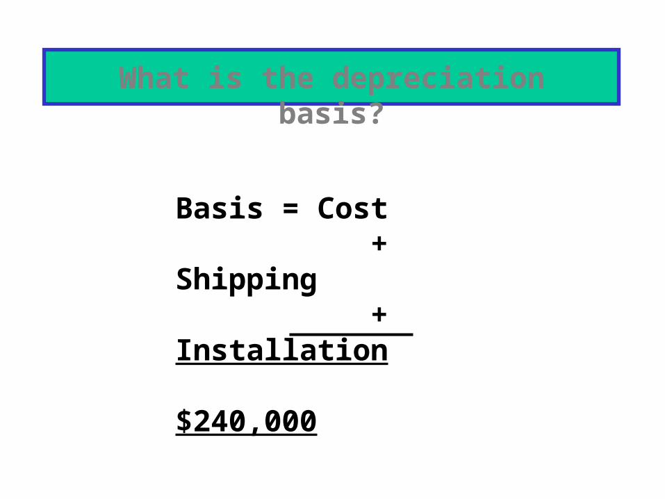
Basis = Cost + Shipping + Installation $240,000
What is the depreciation basis?
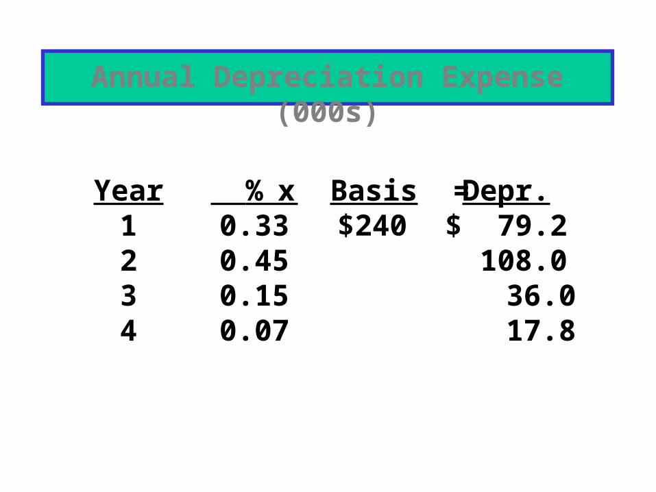
Year1234
% 0.330.450.150.07
Depr.$ 79.2 108.0 36.0 17.8
x Basis =
Annual Depreciation Expense (000s)
$240
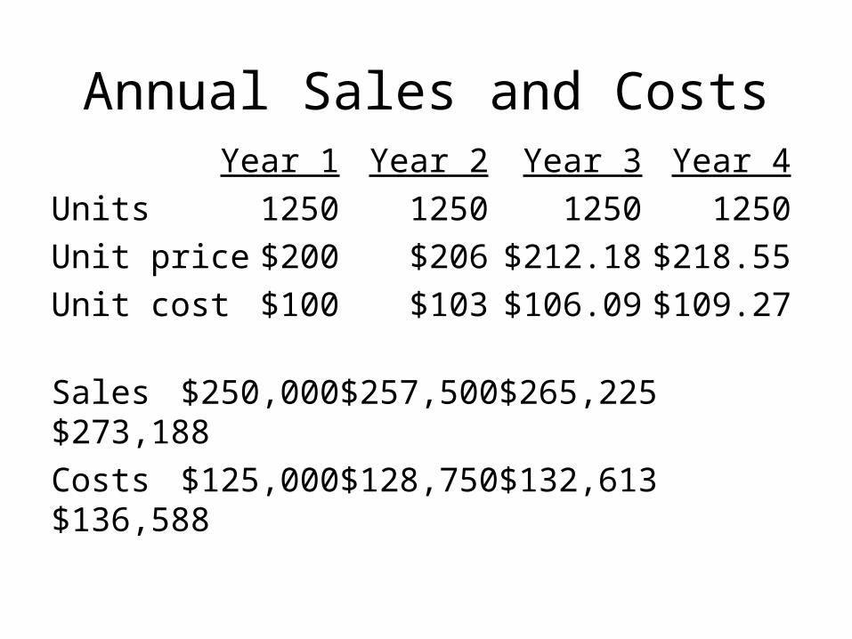
Annual Sales and CostsYear 1 Year 2 Year 3 Year 4
Units 1250 1250 1250 1250
Unit price $200 $206 $212.18 $218.55
Unit cost $100 $103 $106.09 $109.27
Sales $250,000 $257,500 $265,225 $273,188
Costs $125,000 $128,750 $132,613 $136,588
Why is it important to include inflation when estimating cash
flows?• Nominal r > real r. The cost of capital, r,
includes a premium for inflation.• Nominal CF > real CF. This is because
nominal cash flows incorporate inflation.• If you discount real CF with the higher
nominal r, then your NPV estimate is too low.
Continued…
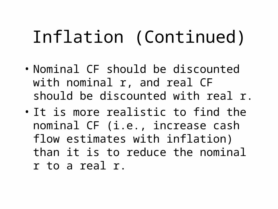
Inflation (Continued)
• Nominal CF should be discounted with nominal r, and real CF should be discounted with real r.
• It is more realistic to find the nominal CF (i.e., increase cash flow estimates with inflation) than it is to reduce the nominal r to a real r.
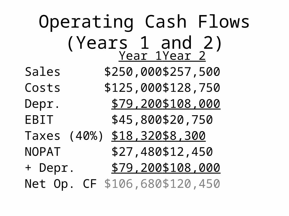
Operating Cash Flows (Years 1 and 2)
Year 1 Year 2Sales $250,000 $257,500Costs $125,000 $128,750Depr. $79,200 $108,000EBIT $45,800 $20,750Taxes (40%) $18,320 $8,300NOPAT $27,480 $12,450+ Depr. $79,200 $108,000Net Op. CF $106,680 $120,450
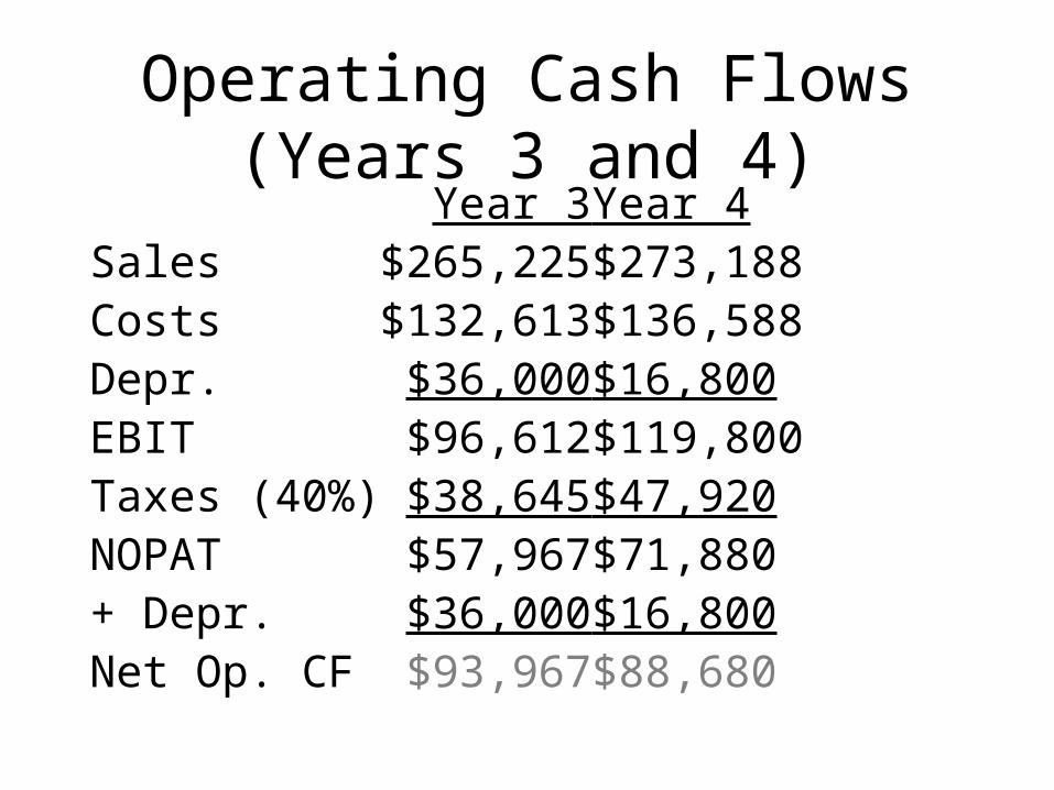
Operating Cash Flows (Years 3 and 4)
Year 3 Year 4Sales $265,225 $273,188Costs $132,613 $136,588Depr. $36,000 $16,800EBIT $96,612 $119,800Taxes (40%) $38,645 $47,920NOPAT $57,967 $71,880+ Depr. $36,000 $16,800Net Op. CF $93,967 $88,680
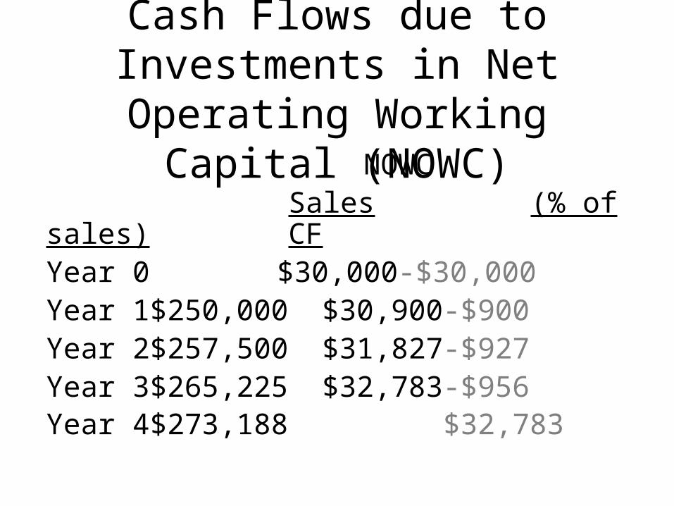
Cash Flows due to Investments in Net Operating Working Capital
(NOWC) NOWC
Sales (% of sales) CFYear 0 $30,000 -$30,000Year 1 $250,000 $30,900 -$900Year 2 $257,500 $31,827 -$927Year 3 $265,225 $32,783 -$956Year 4 $273,188 $32,783
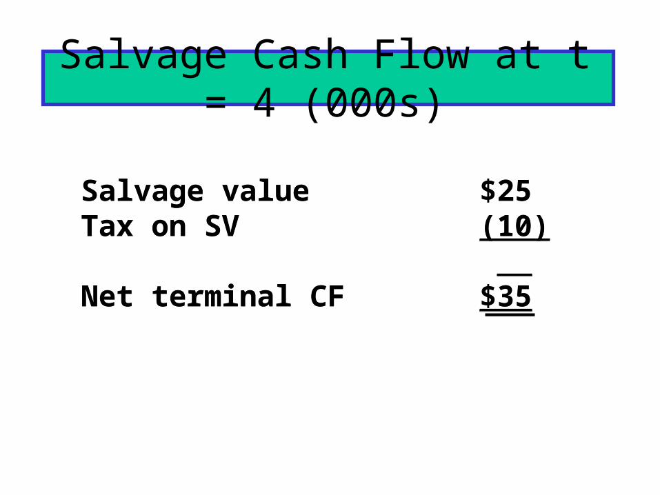
Salvage Cash Flow at t = 4 (000s)
Salvage valueTax on SV
Net terminal CF
Salvage valueTax on SV
Net terminal CF
$25 (10)
$35
$25 (10)
$35
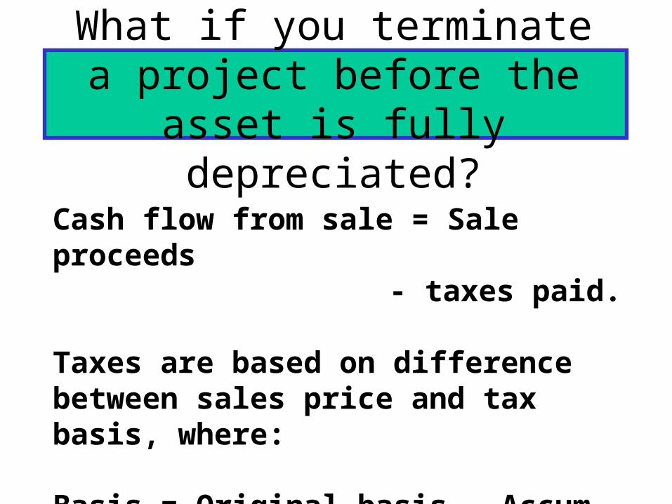
What if you terminate a project before the asset is fully
depreciated?
Cash flow from sale = Sale proceeds- taxes paid.
Taxes are based on difference between sales price and tax basis, where:
Basis = Original basis - Accum. deprec.

• Original basis = $240.• After 3 years = $16.8 remaining.• Sales price = $25.• Tax on sale = 0.4($25-$16.8)
= $3.28.• Cash flow = $25-$3.28=$21.72.
Example: If Sold After 3 Years (000s)
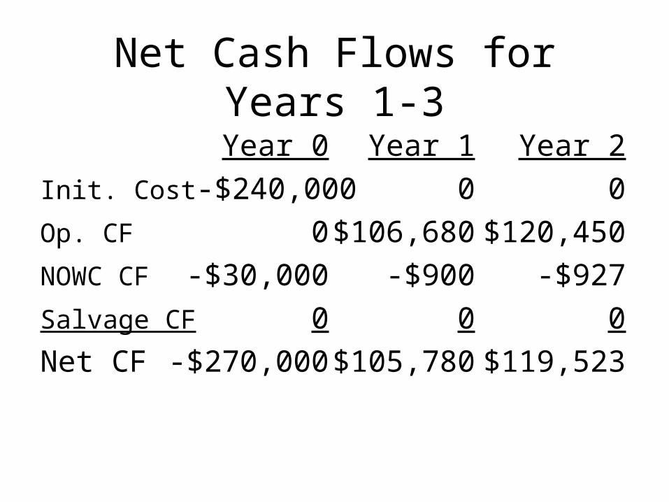
Net Cash Flows for Years 1-3
Year 0 Year 1 Year 2
Init. Cost -$240,000 0 0
Op. CF 0 $106,680 $120,450
NOWC CF -$30,000 -$900 -$927
Salvage CF 0 0 0
Net CF -$270,000 $105,780 $119,523
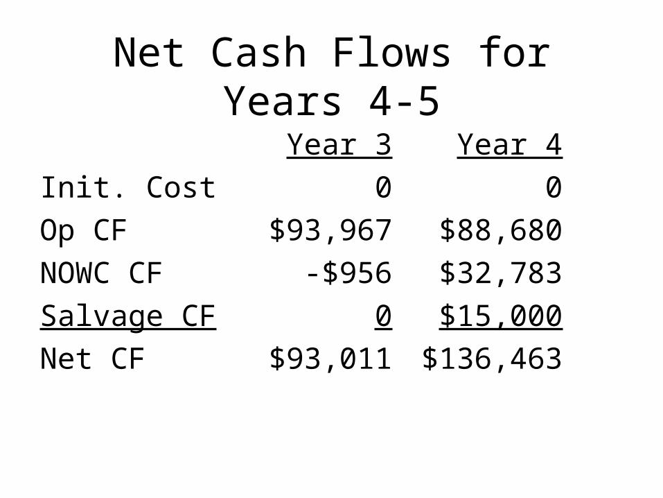
Net Cash Flows for Years 4-5
Year 3 Year 4
Init. Cost 0 0
Op CF $93,967 $88,680
NOWC CF -$956 $32,783
Salvage CF 0 $15,000
Net CF $93,011 $136,463
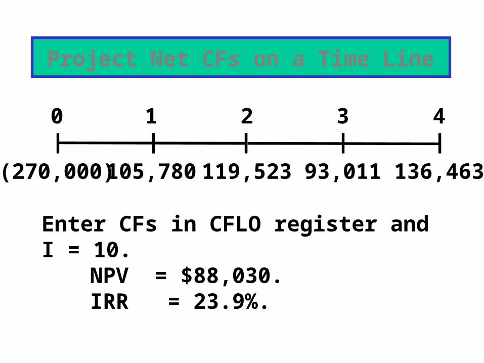
Project Net CFs on a Time Line
Enter CFs in CFLO register and I = 10.NPV = $88,030.IRR = 23.9%.
0 1 2 3 4
(270,000) 105,780 119,523 93,011 136,463

What is the project’s MIRR? (000s)
(270,000)MIRR = ?
0 1 2 3 4
(270,000) 105,780 119,523 93,011 136,463
102,312
144,623
140,793
524,191
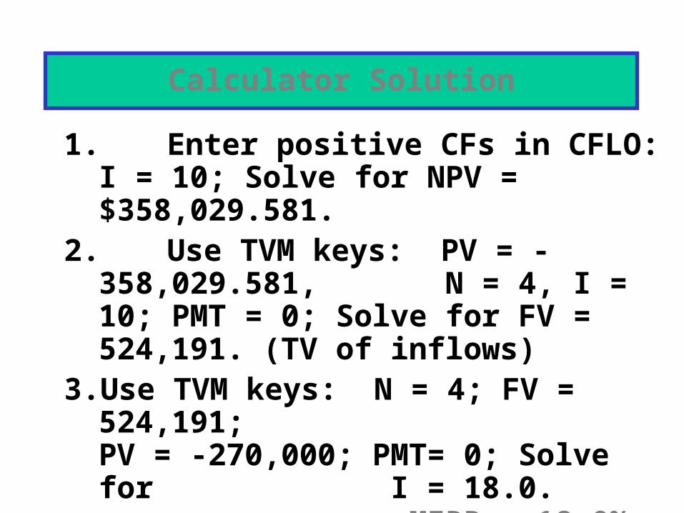
1. Enter positive CFs in CFLO:I = 10; Solve for NPV = $358,029.581.
2. Use TVM keys: PV = -358,029.581, N = 4, I = 10; PMT = 0; Solve for FV = 524,191. (TV of inflows)
3. Use TVM keys: N = 4; FV = 524,191;PV = -270,000; PMT= 0; Solve for I = 18.0. MIRR = 18.0%.
Calculator Solution

What is the project’s payback? (000s)
Cumulative:
Payback = 2 + 44/93 = 2.5 years.
0 1 2 3 4
(270)*
(270)
106
(164)
120
(44)
93
49
136
185
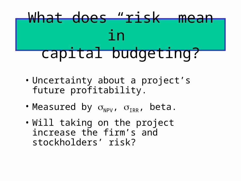
What does “risk” mean in capital budgeting?
• Uncertainty about a project’s future profitability.
• Measured by NPV, IRR, beta.
• Will taking on the project increase the firm’s and stockholders’ risk?

Is risk analysis based on historical data or subjective judgment?
• Can sometimes use historical data, but generally cannot.
• So risk analysis in capital budgeting is usually based on subjective judgments.
What three types of risk are relevant in capital budgeting?
• Stand-alone risk
• Corporate risk
• Market (or beta) risk
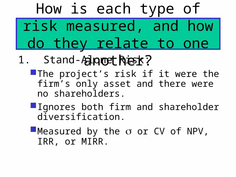
How is each type of risk measured, and how do they relate
to one another?1. Stand-Alone Risk:
The project’s risk if it were the firm’s only asset and there were no shareholders.
Ignores both firm and shareholder diversification. Measured by the or CV of NPV, IRR, or
MIRR.

0 E(NPV)
Probability Density
Flatter distribution,larger , largerstand-alone risk.
Such graphics are increasingly usedby corporations.
NPV
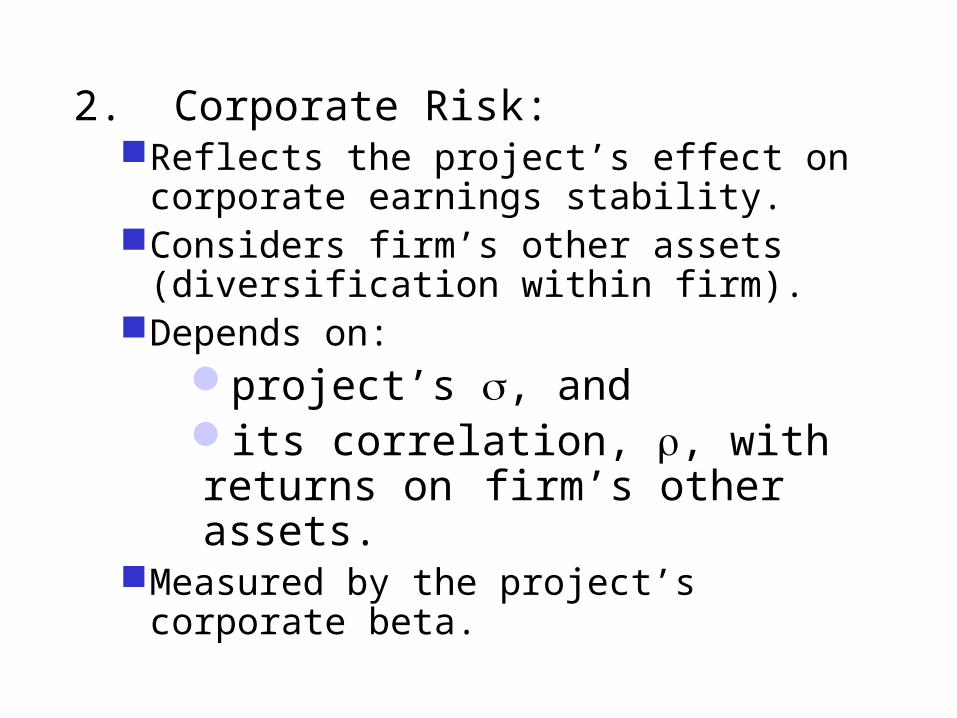
2. Corporate Risk:Reflects the project’s effect on corporate
earnings stability.Considers firm’s other assets (diversification
within firm).Depends on:
project’s , andits correlation, , with returns on
firm’s other assets.Measured by the project’s corporate beta.

Profitability
0 Years
Project X
Total Firm
Rest of Firm
1. Project X is negatively correlated to firm’s other assets.
2. If < 1.0, some diversification benefits.
3. If = 1.0, no diversification effects.
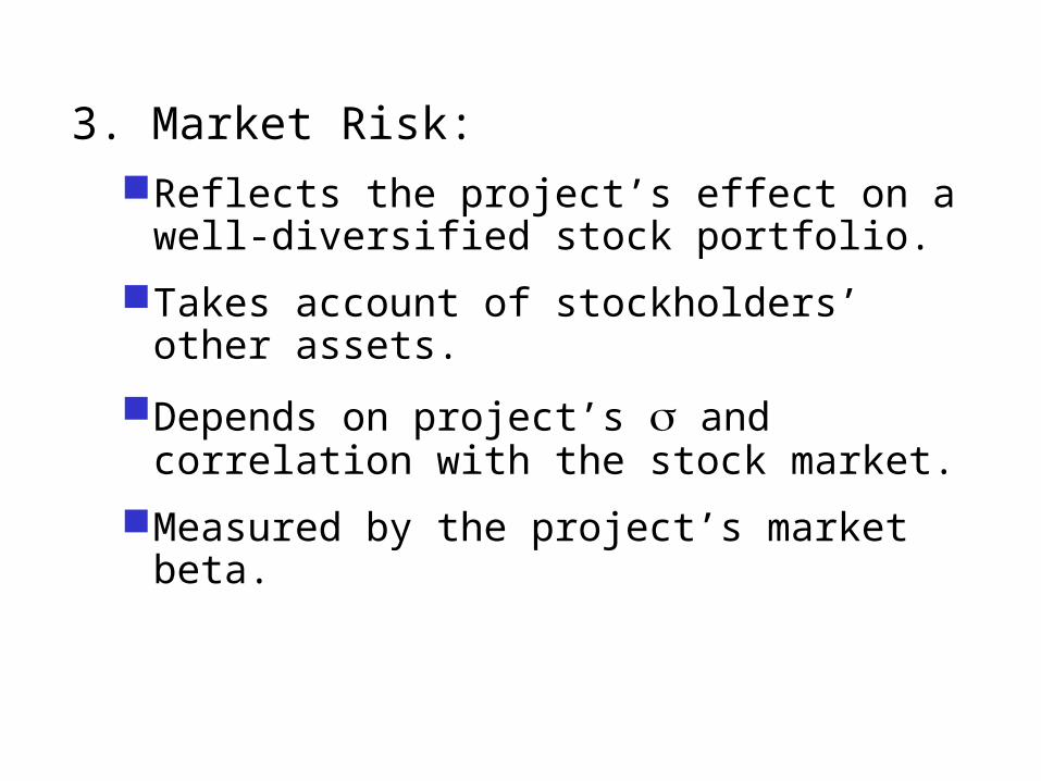
3. Market Risk:
Reflects the project’s effect on a well-diversified stock portfolio.
Takes account of stockholders’ other assets.
Depends on project’s and correlation with the stock market.
Measured by the project’s market beta.

How is each type of risk used?
• Market risk is theoretically best in most situations.
• However, creditors, customers, suppliers, and employees are more affected by corporate risk.
• Therefore, corporate risk is also relevant.
Continued…
• Stand-alone risk is easiest to measure, more intuitive.
• Core projects are highly correlated with other assets, so stand-alone risk generally reflects corporate risk.
• If the project is highly correlated with the economy, stand-alone risk also reflects market risk.
What is sensitivity analysis?
• Shows how changes in a variable such as unit sales affect NPV or IRR.
• Each variable is fixed except one. Change this one variable to see the effect on NPV or IRR.
• Answers “what if” questions, e.g. “What if sales decline by 30%?”

Sensitivity Analysis
-30% $113 $17 $85 -15% $100 $52 $86
0% $88 $88 $88 15% $76 $124 $90 30% $65 $159 $91
Change from Resulting NPV (000s) Base Level r Unit Sales Salvage

-30 -20 -10 Base 10 20 30 Value (%)
88
NPV(000s)
Unit Sales
Salvage
r
• Steeper sensitivity lines show greater risk. Small changes result in large declines in NPV.
• Unit sales line is steeper than salvage value or r, so for this project, should worry most about accuracy of sales forecast.
Results of Sensitivity Analysis

What are the weaknesses ofsensitivity analysis?
• Does not reflect diversification.
• Says nothing about the likelihood of change in a variable, i.e. a steep sales line is not a problem if sales won’t fall.
• Ignores relationships among variables.
Why is sensitivity analysis useful?
• Gives some idea of stand-alone risk.
• Identifies dangerous variables.
• Gives some breakeven information.
What is scenario analysis?
• Examines several possible situations, usually worst case, most likely case, and best case.
• Provides a range of possible outcomes.
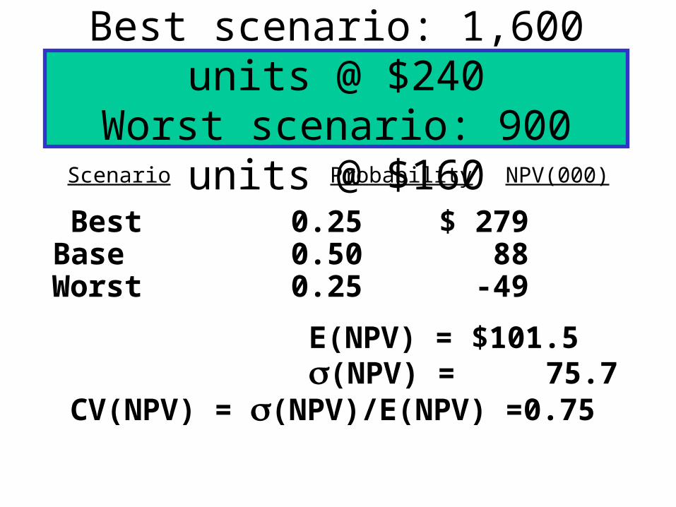
Scenario ProbabilityNPV(000)
Best scenario: 1,600 units @ $240
Worst scenario: 900 units @ $160
Best 0.25 $ 279Base 0.50 88
Worst 0.25 -49
E(NPV) = $101.5(NPV) = 75.7
CV(NPV) = (NPV)/E(NPV) = 0.75
Are there any problems with scenario analysis?
Only considers a few possible out-comes.
Assumes that inputs are perfectly correlated--all “bad” values occur together and all “good” values occur together.
Focuses on stand-alone risk, although subjective adjustments can be made.

What is a simulation analysis?
• A computerized version of scenario analysis which uses continuous probability distributions.
• Computer selects values for each variable based on given probability distributions.
(More...)
• NPV and IRR are calculated.
• Process is repeated many times (1,000 or more).
• End result: Probability distribution of NPV and IRR based on sample of simulated values.
• Generally shown graphically.

Simulation Example• Assume a:
– Normal distribution for unit sales:• Mean = 1,250• Standard deviation = 200
– Triangular distribution for unit price:• Lower bound = $160• Most likely = $200• Upper bound = $250

Simulation Process
• Pick a random variable for unit sales and sale price.
• Substitute these values in the spreadsheet and calculate NPV.
• Repeat the process many times, saving the input variables (units and price) and the output (NPV).
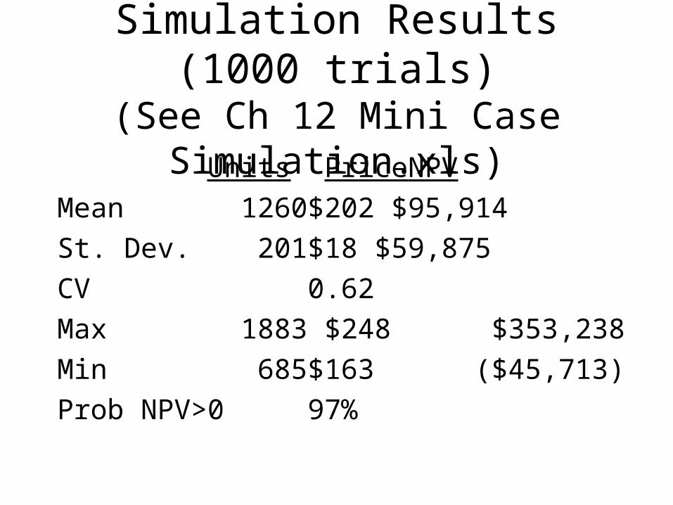
Simulation Results (1000 trials)(See Ch 12 Mini Case
Simulation.xls)Units Price NPV
Mean 1260 $202 $95,914
St. Dev. 201 $18 $59,875
CV 0.62
Max 1883 $248 $353,238
Min 685 $163 ($45,713)
Prob NPV>0 97%

Interpreting the Results
• Inputs are consistent with specificied distributions.– Units: Mean = 1260, St. Dev. = 201.– Price: Min = $163, Mean = $202, Max = $248.
• Mean NPV = $95,914. Low probability of negative NPV (100% - 97% = 3%).
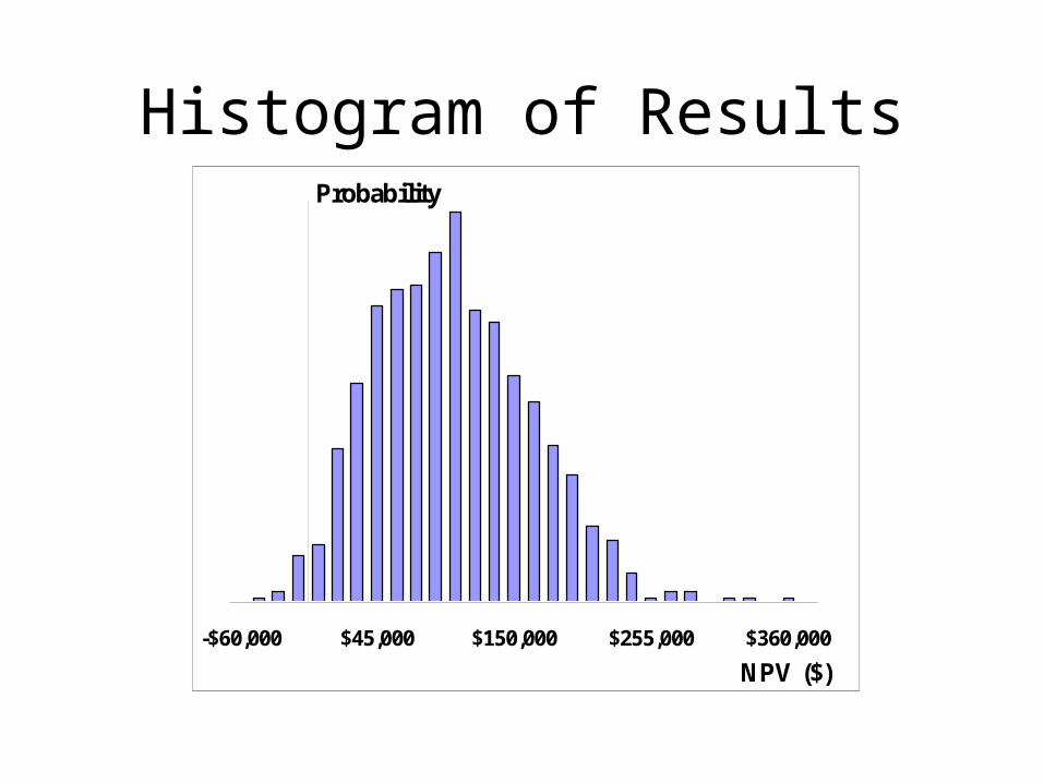
Histogram of Results
-$60,000 $45,000 $150,000 $255,000 $360,000
NPV ($)
Probability
What are the advantages of simulation analysis?
• Reflects the probability distributions of each input.
• Shows range of NPVs, the expected NPV, NPV, and CVNPV.
• Gives an intuitive graph of the risk situation.

What are the disadvantages of simulation?
• Difficult to specify probability distributions and correlations.
• If inputs are bad, output will be bad:“Garbage in, garbage out.”
(More...)
• Sensitivity, scenario, and simulation analyses do not provide a decision rule. They do not indicate whether a project’s expected return is sufficient to compensate for its risk.
• Sensitivity, scenario, and simulation analyses all ignore diversification. Thus they measure only stand-alone risk, which may not be the most relevant risk in capital budgeting.

If the firm’s average project has a CV of 0.2 to 0.4, is this a high-
risk project? What type of risk is being measured?
• CV from scenarios = 0.74, CV from simulation = 0.62. Both are > 0.4, this project has high risk.
• CV measures a project’s stand-alone risk.
• High stand-alone risk usually indicates high corporate and market risks.
With a 3% risk adjustment, should
our project be accepted?
• Project r = 10% + 3% = 13%.
• That’s 30% above base r.
• NPV = $65,371.
• Project remains acceptable after accounting for differential (higher) risk.
Should subjective risk factors be considered?
• Yes. A numerical analysis may not capture all of the risk factors inherent in the project.
• For example, if the project has the potential for bringing on harmful lawsuits, then it might be riskier than a standard analysis would indicate.
What is capital budgeting?
• Analysis of potential projects.
• Long-term decisions; involve large expenditures.
• Very important to firm’s future.
Steps in Capital Budgeting
• Estimate cash flows (inflows & outflows).
• Assess risk of cash flows.
• Determine r = WACC for project.
• Evaluate cash flows.
What is the difference between independent and mutually
exclusive projects?Projects are:
independent, if the cash flows of one are unaffected by the acceptance of the other.
mutually exclusive, if the cash flows of one can be adversely impacted by the acceptance of the other.
What is the payback period?
The number of years required to recover a project’s cost,
or how long does it take to get the business’s money back?
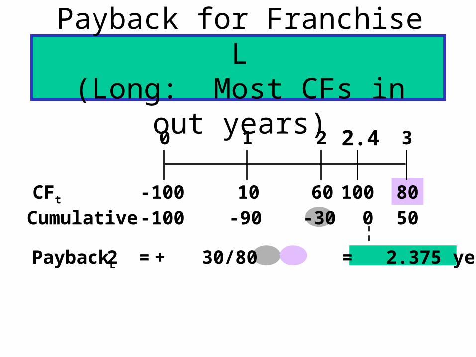
Payback for Franchise L(Long: Most CFs in out years)
10 8060
0 1 2 3
-100
=
CFt
Cumulative -100 -90 -30 50
PaybackL 2 + 30/80 = 2.375 years
0100
2.4
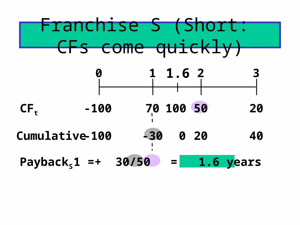
Franchise S (Short: CFs come quickly)
70 2050
0 1 2 3
-100CFt
Cumulative -100 -30 20 40
PaybackS 1 + 30/50 = 1.6 years
100
0
1.6
=

Strengths of Payback:
1. Provides an indication of a project’s risk and liquidity.
2. Easy to calculate and understand.
Weaknesses of Payback:
1. Ignores the TVM.
2. Ignores CFs occurring after the payback period.

10 8060
0 1 2 3
CFt
Cumulative -100 -90.91 -41.32 18.79
Discountedpayback 2 + 41.32/60.11 = 2.7 yrs
Discounted Payback: Uses discountedrather than raw CFs.
PVCFt -100
-100
10%
9.09 49.59 60.11
=
Recover invest. + cap. costs in 2.7 yrs.

.
10t
tn
t r
CFNPV
NPV: Sum of the PVs of inflows and outflows.
Cost often is CF0 and is negative.
.
10
1
CFr
CFNPV t
tn
t

What’s Franchise L’s NPV?
10 8060
0 1 2 310%
Project L:
-100.00
9.09
49.59
60.1118.79 = NPVL NPVS = $19.98.
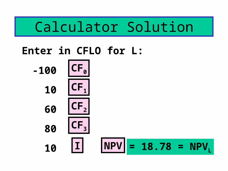
Calculator Solution
Enter in CFLO for L:
-100
10
60
80
10
CF0
CF1
NPV
CF2
CF3
I = 18.78 = NPVL

Rationale for the NPV Method
NPV = PV inflows - Cost= Net gain in wealth.
Accept project if NPV > 0.
Choose between mutually exclusive projects on basis ofhigher NPV. Adds most value.
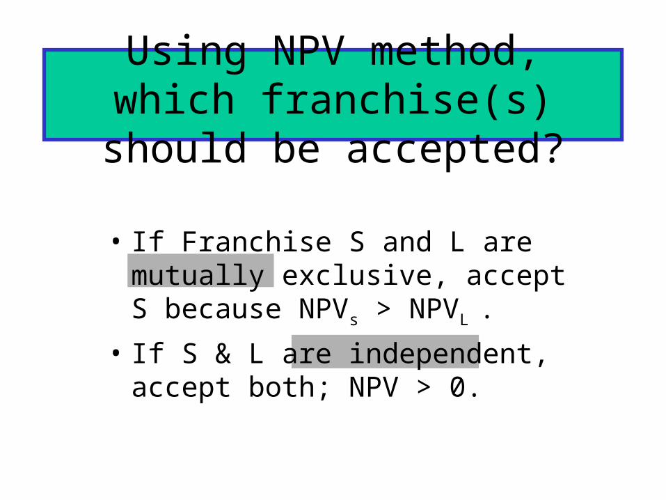
Using NPV method, which franchise(s) should be accepted?
• If Franchise S and L are mutually exclusive, accept S because NPVs > NPVL .
• If S & L are independent, accept both; NPV > 0.
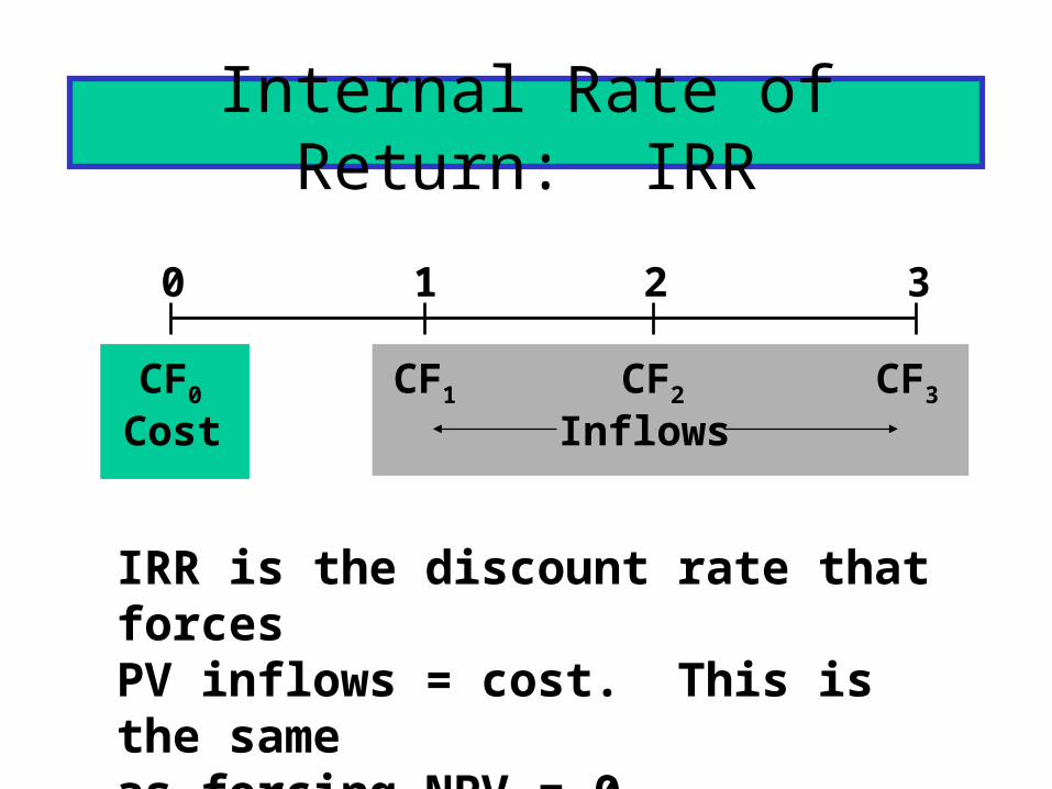
Internal Rate of Return: IRR
0 1 2 3
CF0 CF1 CF2 CF3
Cost Inflows
IRR is the discount rate that forcesPV inflows = cost. This is the sameas forcing NPV = 0.
.
10
NPVr
CFt
tn
t
t
nt
t
CF
IRR
0 10.
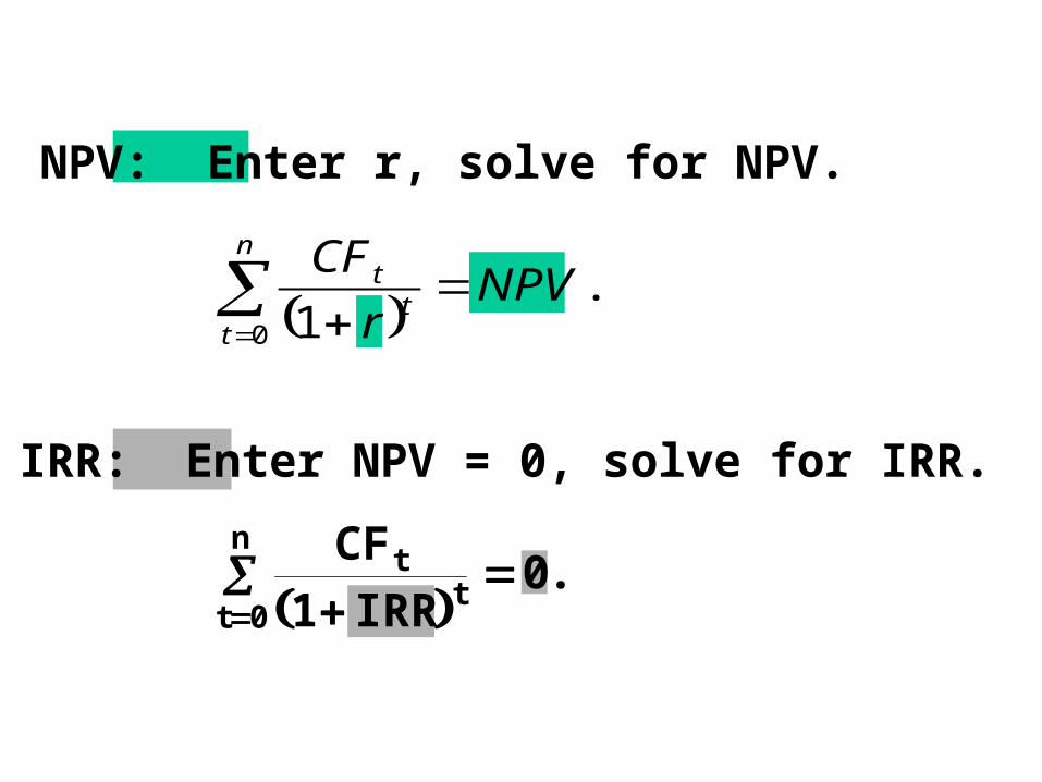
NPV: Enter r, solve for NPV.
IRR: Enter NPV = 0, solve for IRR.

What’s Franchise L’s IRR?
10 8060
0 1 2 3IRR = ?
-100.00
PV3
PV2
PV1
0 = NPV
Enter CFs in CFLO, then press IRR:IRRL = 18.13%. IRRS = 23.56%.

40 40 40
0 1 2 3IRR = ?
Find IRR if CFs are constant:
-100
Or, with CFLO, enter CFs and press IRR = 9.70%.
3 -100 40 0
9.70%N I/YR PV PMT FV
INPUTS
OUTPUT
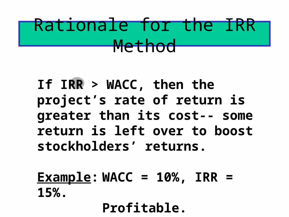
Rationale for the IRR Method
If IRR > WACC, then the project’s rate of return is greater than its cost-- some return is left over to boost stockholders’ returns.
Example: WACC = 10%, IRR = 15%.Profitable.
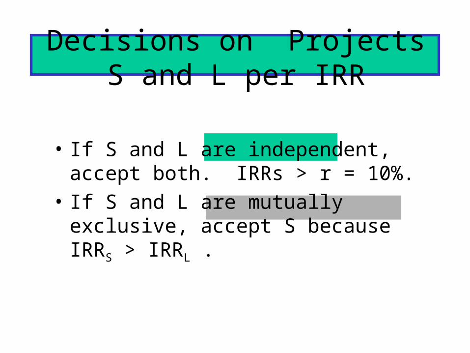
Decisions on Projects S and L per IRR
• If S and L are independent, accept both. IRRs > r = 10%.
• If S and L are mutually exclusive, accept S because IRRS > IRRL .

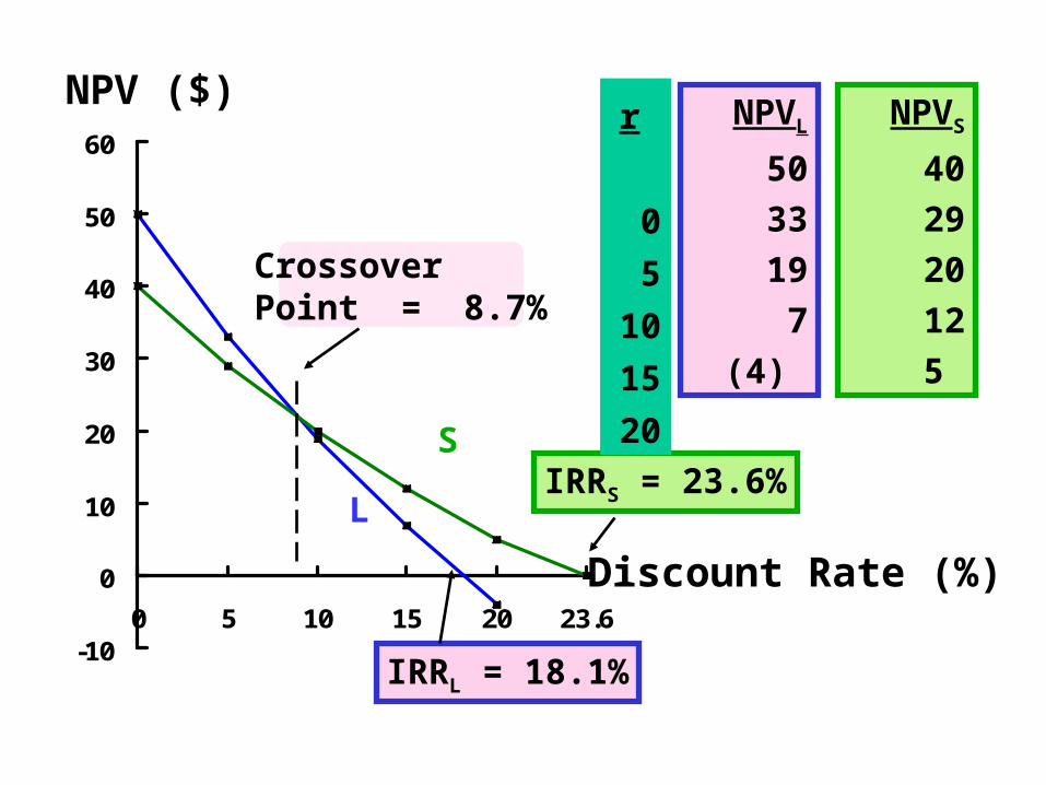
Construct NPV Profiles
Enter CFs in CFLO and find NPVL andNPVS at different discount rates:
r
0
5
10
15
20
NPVL
50
33
19
7
NPVS
40
29
20
12
5 (4)
-10
0
10
20
30
40
50
60
0 5 10 15 20 23.6
NPV ($)
Discount Rate (%)
IRRL = 18.1%
IRRS = 23.6%
Crossover Point = 8.7%
r
0
5
10
15
20
NPVL
50
33
19
7
(4)
NPVS
40
29
20
12
5
S
L

NPV and IRR always lead to the same accept/reject decision for independent projects:
r > IRRand NPV < 0.
Reject.
NPV ($)
r (%)IRR
IRR > rand NPV > 0
Accept.
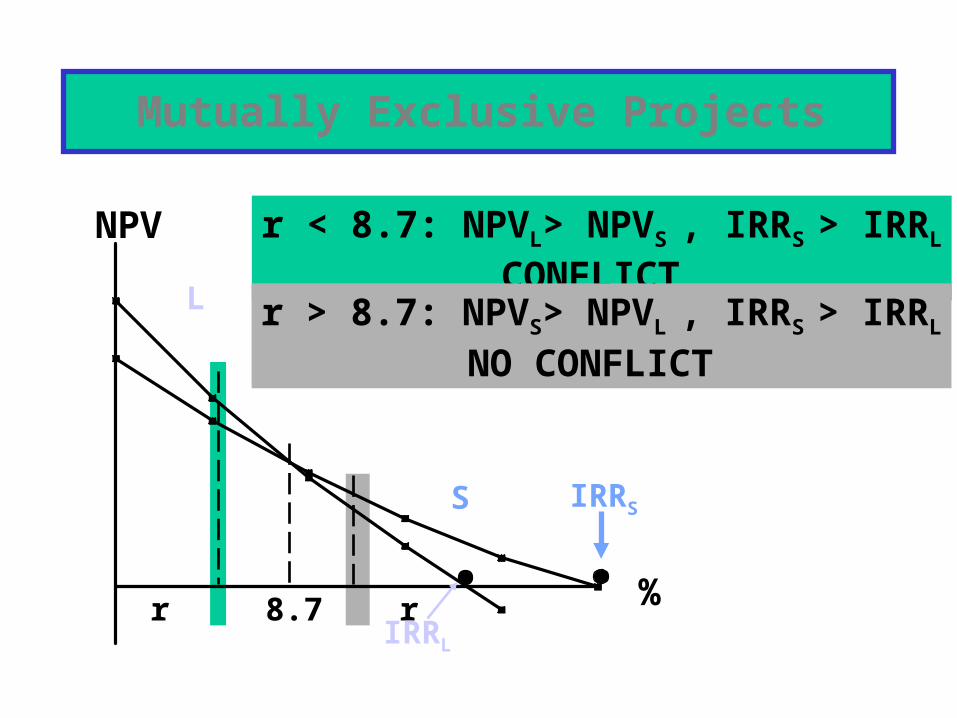
Mutually Exclusive Projects
r 8.7 r
NPV
%
IRRS
IRRL
L
S
r < 8.7: NPVL> NPVS , IRRS > IRRL
CONFLICT r > 8.7: NPVS> NPVL , IRRS > IRRL
NO CONFLICT

To Find the Crossover Rate
1. Find cash flow differences between the projects. See data at beginning of the case.
2. Enter these differences in CFLO register, then press IRR. Crossover rate = 8.68%, rounded to 8.7%.
3. Can subtract S from L or vice versa, but better to have first CF negative.
4. If profiles don’t cross, one project dominates the other.
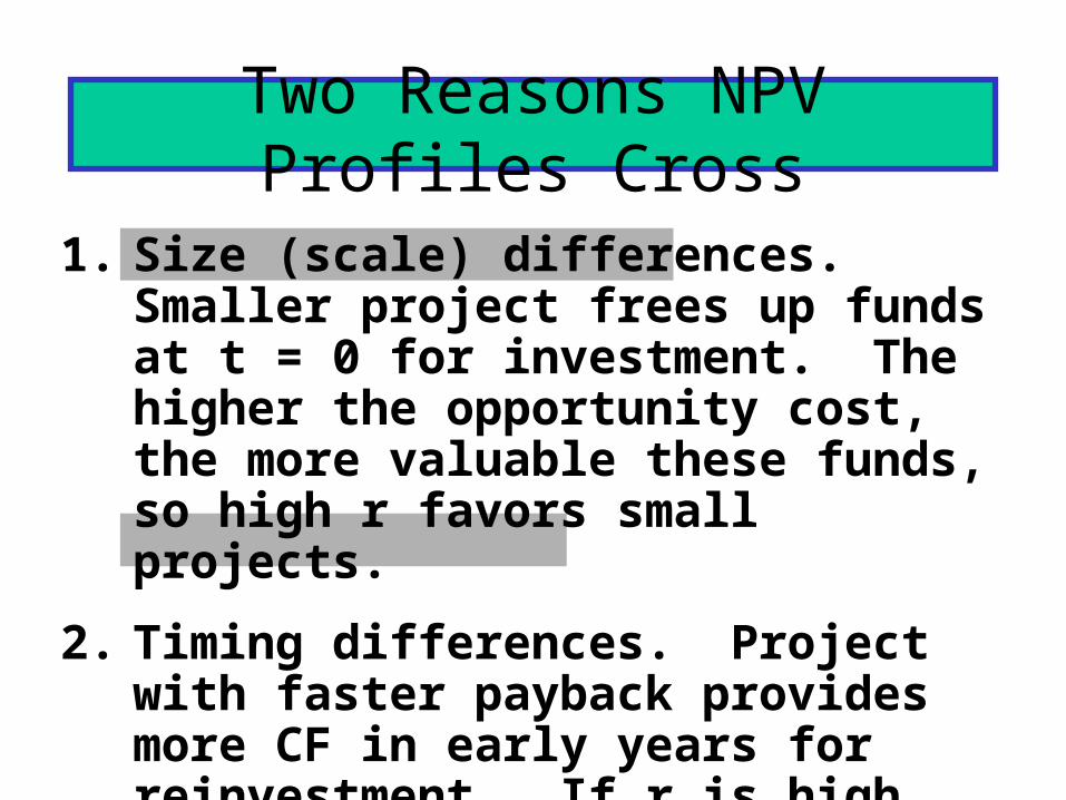
Two Reasons NPV Profiles Cross
1. Size (scale) differences. Smaller project frees up funds at t = 0 for investment. The higher the opportunity cost, the more valuable these funds, so high r favors small projects.
2. Timing differences. Project with faster payback provides more CF in early years for reinvestment. If r is high, early CF especially good, NPVS > NPVL.
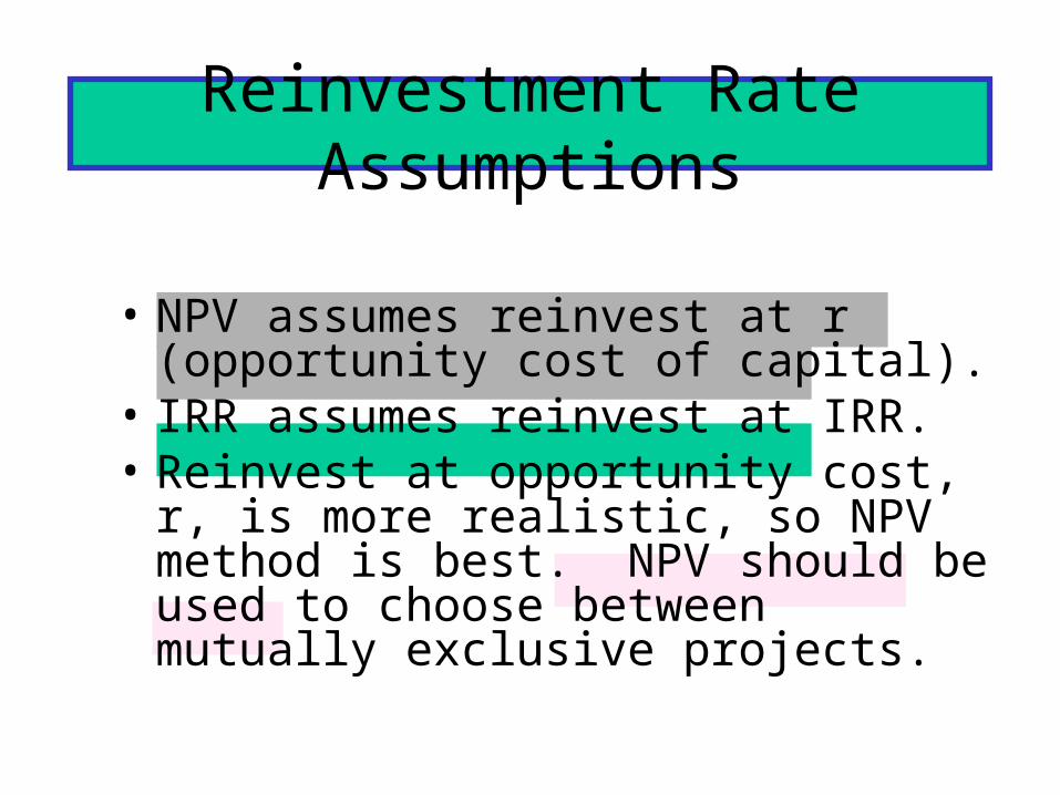
Reinvestment Rate Assumptions
• NPV assumes reinvest at r (opportunity cost of capital).
• IRR assumes reinvest at IRR.• Reinvest at opportunity cost, r, is more
realistic, so NPV method is best. NPV should be used to choose between mutually exclusive projects.
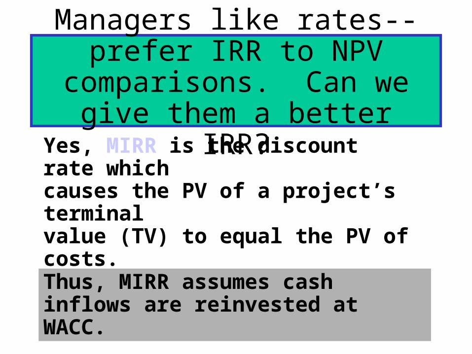
Managers like rates--prefer IRR to NPV comparisons. Can we
give them a better IRR?Yes, MIRR is the discount rate whichcauses the PV of a project’s terminalvalue (TV) to equal the PV of costs.TV is found by compounding inflowsat WACC.
Thus, MIRR assumes cash inflows are reinvested at WACC.
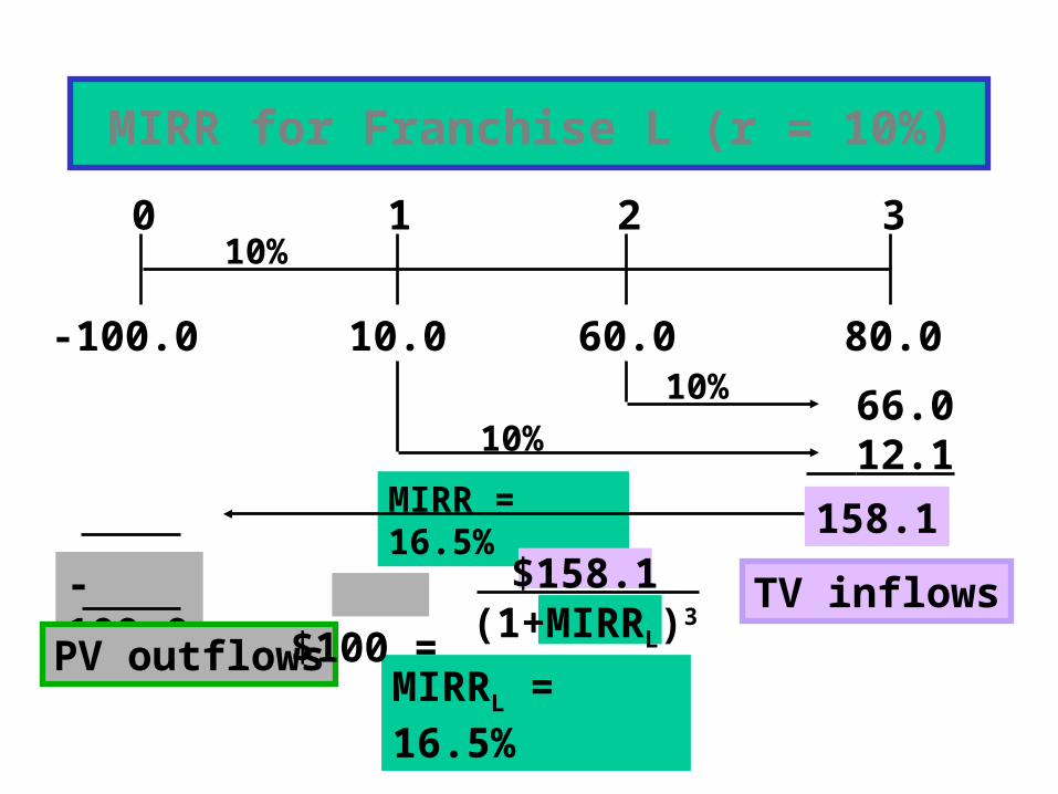
MIRR = 16.5%
10.0 80.060.0
0 1 2 310%
66.0 12.1
158.1
MIRR for Franchise L (r = 10%)
-100.010%
10%
TV inflows-100.0
PV outflowsMIRRL = 16.5%
$100 = $158.1
(1+MIRRL)3

To find TV with 10B, enter in CFLO:
I = 10
NPV = 118.78 = PV of inflows.
Enter PV = -118.78, N = 3, I = 10, PMT = 0.Press FV = 158.10 = FV of inflows.
Enter FV = 158.10, PV = -100, PMT = 0, N = 3.Press I = 16.50% = MIRR.
CF0 = 0, CF1 = 10, CF2 = 60, CF3 = 80

Why use MIRR versus IRR?
MIRR correctly assumes reinvestment at opportunity cost = WACC. MIRR also avoids the problem of multiple IRRs.
Managers like rate of return comparisons, and MIRR is better for this than IRR.
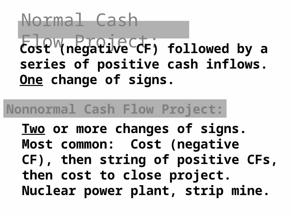
Normal Cash Flow Project:Cost (negative CF) followed by a
series of positive cash inflows. One change of signs.
Nonnormal Cash Flow Project:
Two or more changes of signs.Most common: Cost (negativeCF), then string of positive CFs,then cost to close project.Nuclear power plant, strip mine.
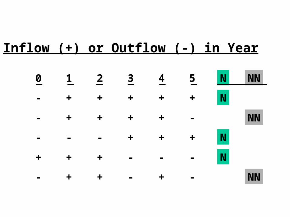
Inflow (+) or Outflow (-) in Year
0 1 2 3 4 5 N NN
- + + + + + N
- + + + + - NN
- - - + + + N
+ + + - - - N
- + + - + - NN
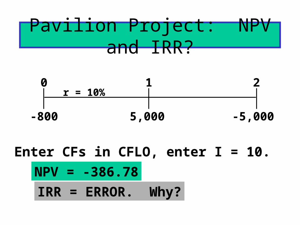
Pavilion Project: NPV and IRR?
5,000 -5,000
0 1 2r = 10%
-800
Enter CFs in CFLO, enter I = 10.
NPV = -386.78
IRR = ERROR. Why?

We got IRR = ERROR because there are 2 IRRs. Nonnormal CFs--two signchanges. Here’s a picture:
NPV Profile
450
-800
0400100
IRR2 = 400%
IRR1 = 25%
r
NPV

Logic of Multiple IRRs
1. At very low discount rates, the PV of CF2 is large & negative, so NPV < 0.
2. At very high discount rates, the PV of both CF1 and CF2 are low, so CF0 dominates and again NPV < 0.
3. In between, the discount rate hits CF2 harder than CF1, so NPV > 0.
4. Result: 2 IRRs.
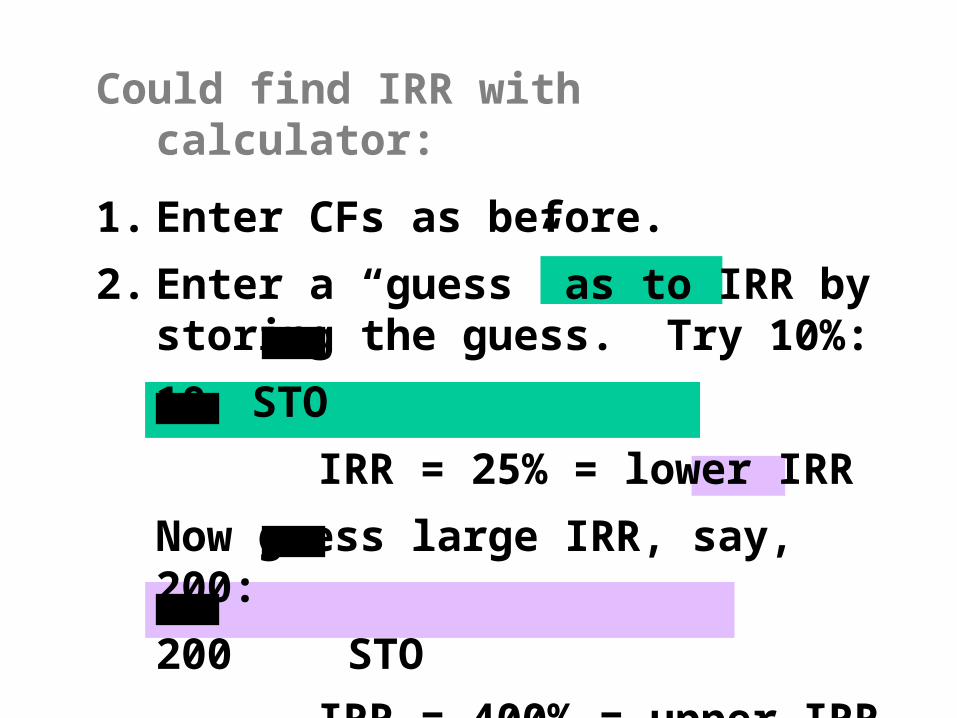
Could find IRR with calculator:
1. Enter CFs as before.
2. Enter a “guess” as to IRR by storing the guess. Try 10%:
10 STO
IRR = 25% = lower IRR
Now guess large IRR, say, 200:
200 STO
IRR = 400% = upper IRR
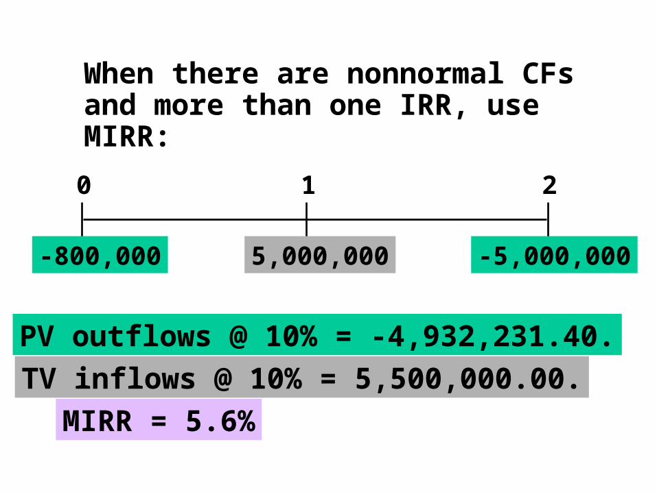
When there are nonnormal CFs and more than one IRR, use MIRR:
0 1 2
-800,000 5,000,000 -5,000,000
PV outflows @ 10% = -4,932,231.40.
TV inflows @ 10% = 5,500,000.00.
MIRR = 5.6%
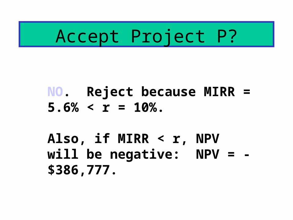
Accept Project P?
NO. Reject because MIRR = 5.6% < r = 10%.
Also, if MIRR < r, NPV will be negative: NPV = -$386,777.
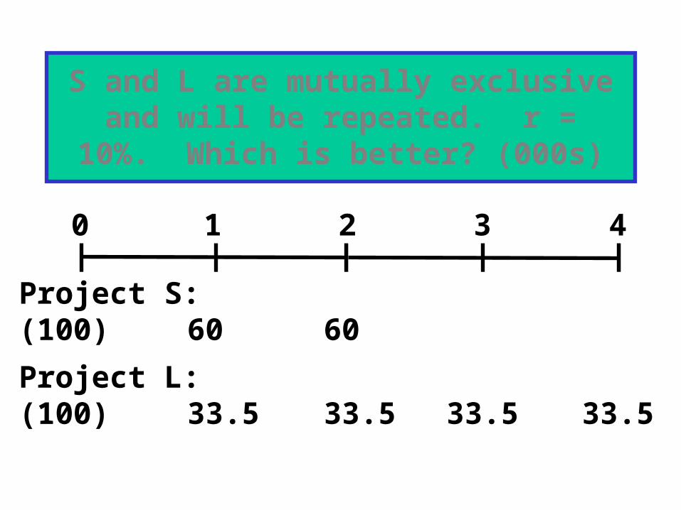
S and L are mutually exclusive and will be repeated. r = 10%. Which is
better? (000s)
0 1 2 3 4
Project S:(100)
Project L:(100)
60
33.5
60
33.5 33.5 33.5

S LCF0 -100,000 -100,000CF1 60,000 33,500Nj 2 4I 10 10
NPV 4,132 6,190
NPVL > NPVS. But is L better?Can’t say yet. Need to perform common life analysis.
• Note that Project S could be repeated after 2 years to generate additional profits.
• Can use either replacement chain or equivalent annual annuity analysis to make decision.
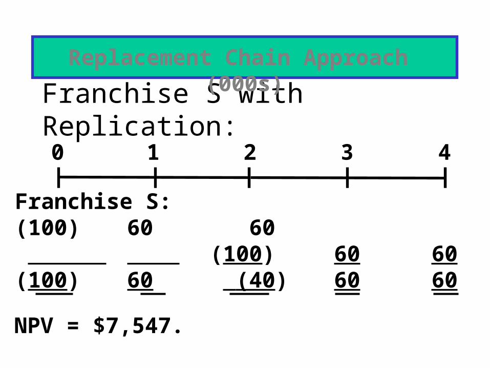
Franchise S with Replication:
NPV = $7,547.
Replacement Chain Approach (000s)
0 1 2 3 4
Franchise S:(100) (100)
60 60
60(100) (40)
6060
6060

Compare to Franchise L NPV = $6,190.Compare to Franchise L NPV = $6,190.
Or, use NPVs:
0 1 2 3 4
4,1323,4157,547
4,13210%

If the cost to repeat S in two years rises to $105,000, which is best? (000s)
NPVS = $3,415 < NPVL = $6,190.Now choose L.NPVS = $3,415 < NPVL = $6,190.Now choose L.
0 1 2 3 4
Franchise S:(100)
60 60(105) (45)
60 60

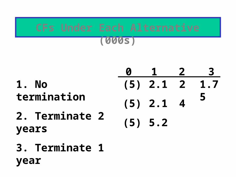
Year0123
CF ($5,000) 2,100 2,000 1,750
Salvage Value $5,000 3,100 2,000 0
Consider another project with a 3-year life. If terminated prior to Year 3, the machinery will have positive salvage
value.
1.751. No termination
2. Terminate 2 years
3. Terminate 1 year
(5)
(5)
(5)
2.1
2.1
5.2
2
4
0 1 2 3
CFs Under Each Alternative (000s)

NPV(no) = -$123.
NPV(2) = $215.
NPV(1) = -$273.
Assuming a 10% cost of capital, what is the project’s optimal, or economic life?
• The project is acceptable only if operated for 2 years.
• A project’s engineering life does not always equal its economic life.
Conclusions
Choosing the Optimal Capital Budget
• Finance theory says to accept all positive NPV projects.
• Two problems can occur when there is not enough internally generated cash to fund all positive NPV projects:
– An increasing marginal cost of capital.
– Capital rationing

Increasing Marginal Cost of Capital
• Externally raised capital can have large flotation costs, which increase the cost of capital.
• Investors often perceive large capital budgets as being risky, which drives up the cost of capital.
(More...)
• If external funds will be raised, then the NPV of all projects should be estimated using this higher marginal cost of capital.
Capital Rationing
• Capital rationing occurs when a company chooses not to fund all positive NPV projects.
• The company typically sets an upper limit on the total amount of capital expenditures that it will make in the upcoming year.
(More...)
Reason: Companies want to avoid the direct costs (i.e., flotation costs) and the indirect costs of issuing new capital.
Solution: Increase the cost of capital by enough to reflect all of these costs, and then accept all projects that still have a positive NPV with the higher cost of capital.
(More...)
Reason: Companies don’t have enough managerial, marketing, or engineering staff to implement all positive NPV projects.
Solution: Use linear programming to maximize NPV subject to not exceeding the constraints on staffing.
(More...)

Reason: Companies believe that the project’s managers forecast unreasonably high cash flow estimates, so companies “filter” out the worst projects by limiting the total amount of projects that can be accepted.
Solution: Implement a post-audit process and tie the managers’ compensation to the subsequent performance of the project.
Corporate Valuation: List the two types of assets that a
company owns.• Assets-in-place (page 358)
• Financial, or nonoperating, assets

Assets-in-Place
• Assets-in-place are tangible, such as buildings, machines, inventory.
• Usually they are expected to grow.
• They generate free cash flows.
• The PV of their expected future free cash flows, discounted at the WACC, is the value of operations.
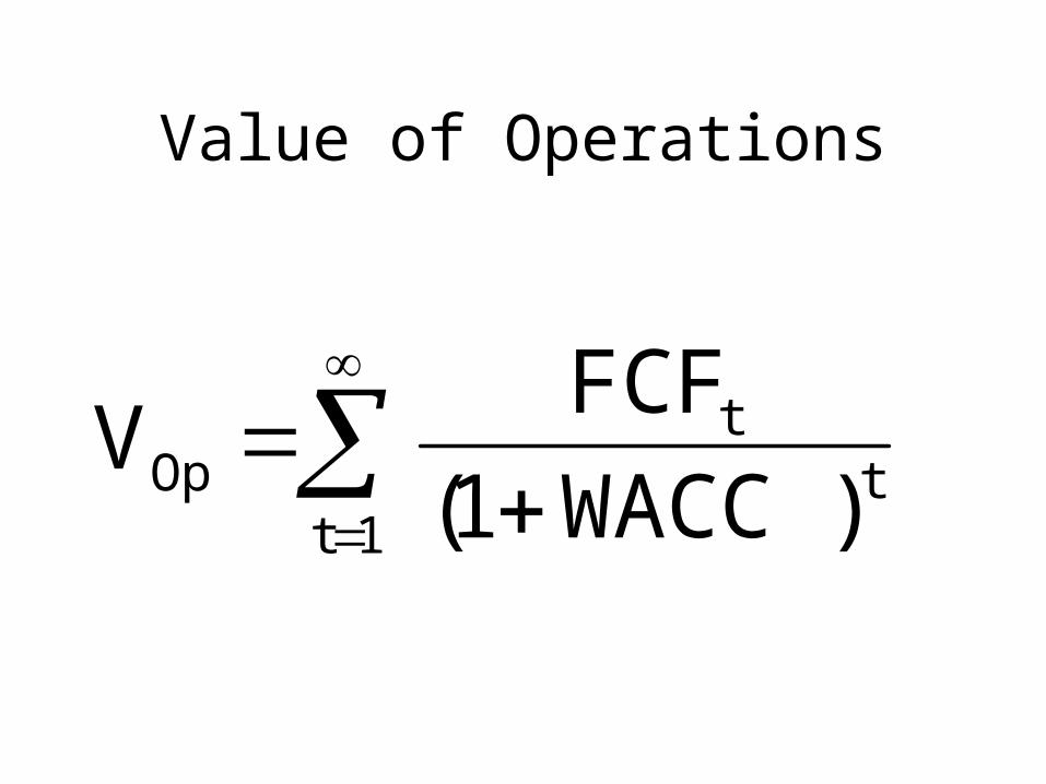
Value of Operations
1tt
tOp )WACC1(
FCFV

Nonoperating Assets
• Marketable securities
• Ownership of non-controlling interest in another company
• Value of nonoperating assets usually is very close to figure that is reported on balance sheets.
Total Corporate Value
• Total corporate value is sum of:– Value of operations– Value of nonoperating assets
Claims on Corporate Value
• Debtholders have first claim.
• Preferred stockholders have the next claim.
• Any remaining value belongs to stockholders.
Applying the Corporate Valuation Model
• Forecast the financial statements, as shown in Chapter 8.
• Calculate the projected free cash flows.
• Model can be applied to a company that does not pay dividends, a privately held company, or a division of a company, since FCF can be calculated for each of these situations.

Data for Valuation• FCF0 = $20 million
• WACC = 10%
• g = 5%
• Marketable securities = $100 million
• Debt = $200 million
• Preferred stock = $50 million
• Book value of equity = $210 million

Value of Operations: Constant Growth
Suppose FCF grows at constant rate g.
1tt
t0
1tt
tOp
WACC1
)g1(FCF
WACC1
FCFV
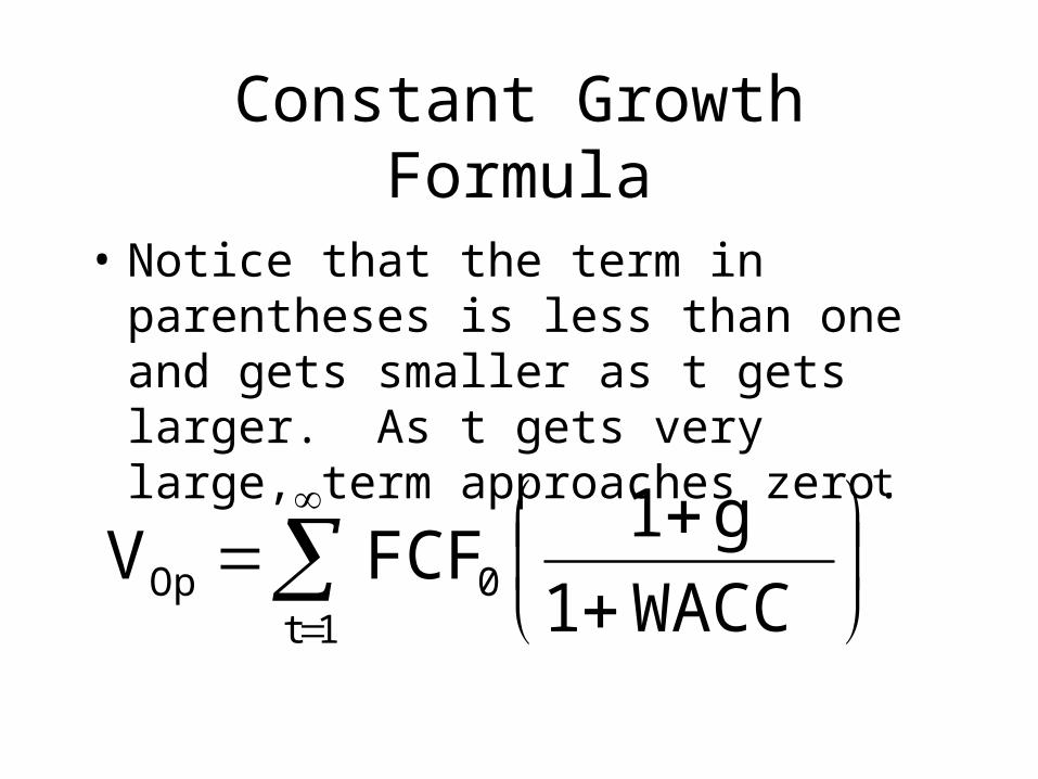
Constant Growth Formula
• Notice that the term in parentheses is less than one and gets smaller as t gets larger. As t gets very large, term approaches zero.
1t
t
0Op WACC1
g1FCFV

Constant Growth Formula (Cont.)
• The summation can be replaced by a single formula:
gWACC
)g1(FCF
gWACC
FCFV
0
1Op

Find Value of Operations
42005.010.0
)05.01(20V
gWACC
)g1(FCFV
Op
0Op

Value of Equity• Sources of Corporate Value
– Value of operations = $420– Value of non-operating assets = $100
• Claims on Corporate Value– Value of Debt = $200– Value of Preferred Stock = $50– Value of Equity = ?
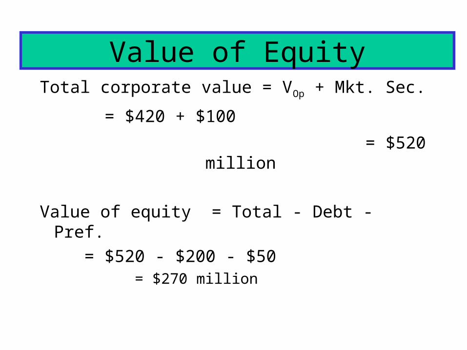
Value of EquityTotal corporate value = VOp + Mkt. Sec.
= $420 + $100
= $520 million
Value of equity = Total - Debt - Pref.
= $520 - $200 - $50 = $270 million
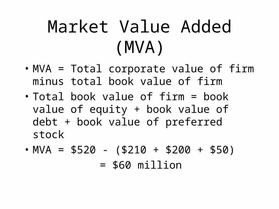
Market Value Added (MVA)
• MVA = Total corporate value of firm minus total book value of firm
• Total book value of firm = book value of equity + book value of debt + book value of preferred stock
• MVA = $520 - ($210 + $200 + $50)
= $60 million

Breakdown of Corporate Value
0
100
200
300
400
500
600
Sourcesof Value
Claimson Value
Marketvs. Book
MVA
Book equity
Equity (Market)
Preferred stock
Debt
Marketablesecurities
Value of operations
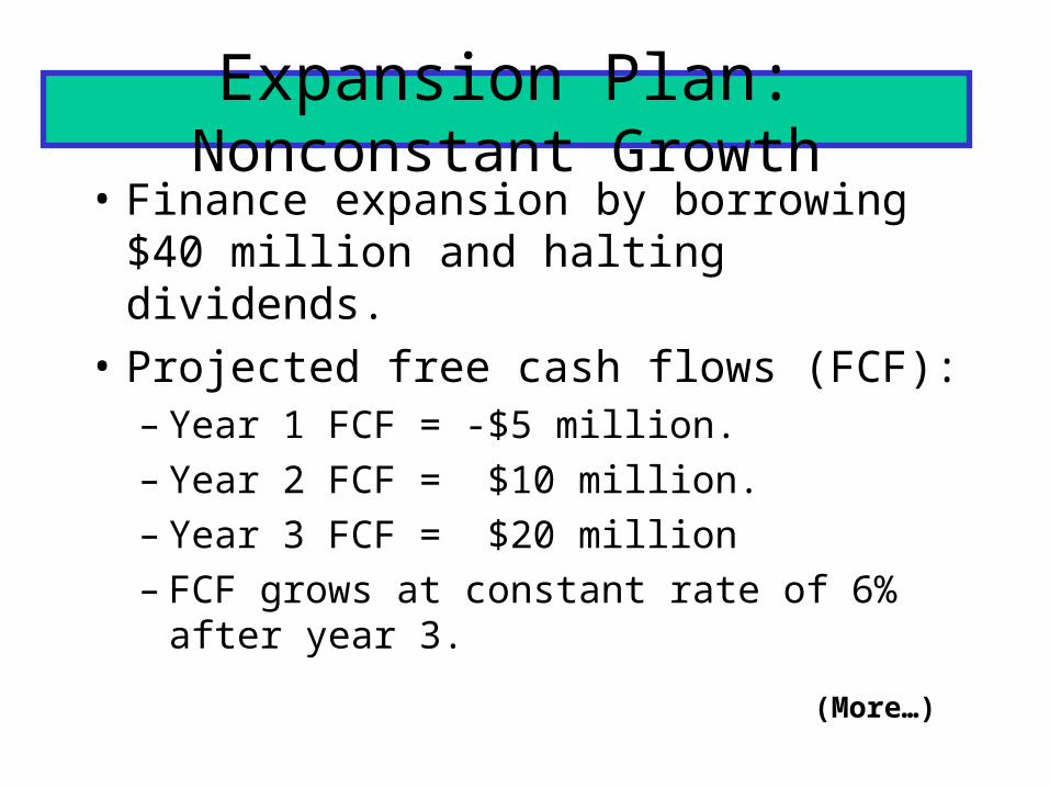
Expansion Plan: Nonconstant Growth
• Finance expansion by borrowing $40 million and halting dividends.
• Projected free cash flows (FCF):– Year 1 FCF = -$5 million.– Year 2 FCF = $10 million.– Year 3 FCF = $20 million– FCF grows at constant rate of 6% after year 3.
(More…)
• The weighted average cost of capital, rc, is 10%.
• The company has 10 million shares of stock.
Horizon Value
• Free cash flows are forecast for three years in this example, so the forecast horizon is three years.
• Growth in free cash flows is not constant during the forecast,so we can’t use the constant growth formula to find the value of operations at time 0.
Horizon Value (Cont.)
• Growth is constant after the horizon (3 years), so we can modify the constant growth formula to find the value of all free cash flows beyond the horizon, discounted back to the horizon.

Horizon Value Formula
• Horizon value is also called terminal value, or continuing value.
gWACC
)g1(FCFVHV t
ttimeatOp
Vop at 3
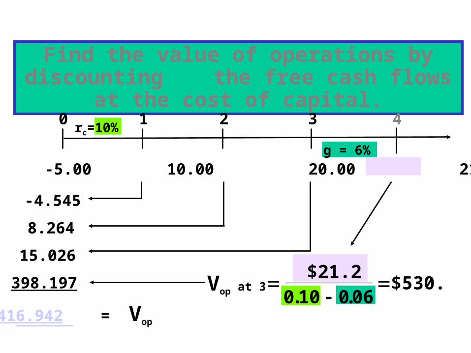
Find the value of operations by discounting the free cash flows at the cost of capital.
0
-4.545
8.264
15.026
398.197
1 2 3 4rc=10%
416.942 = Vop
g = 6%
FCF= -5.00 10.00 20.00 21.2
$21.2. .
$530.10 0 06
0

Find the price per share of common stock.
Value of equity = Value of operations
- Value of debt
= $416.94 - $40
= $376.94 million.
Price per share = $376.94 /10 = $37.69.

Value-Based Management (VBM)
• VBM is the systematic application of the corporate valuation model to all corporate decisions and strategic initiatives.
• The objective of VBM is to increase Market Value Added (MVA)
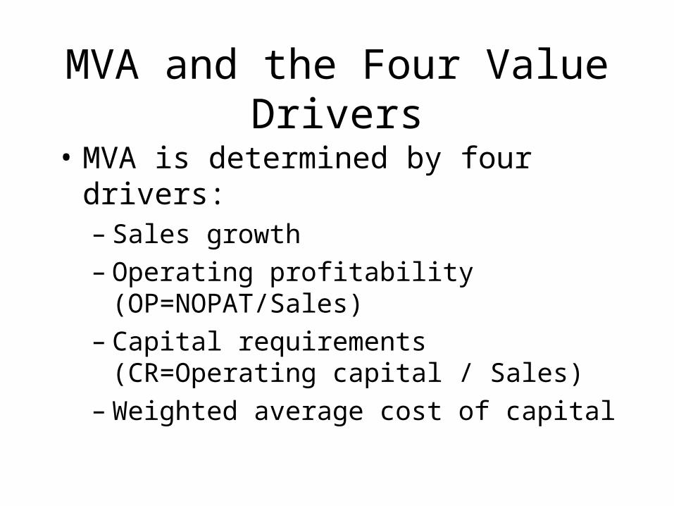
MVA and the Four Value Drivers
• MVA is determined by four drivers:– Sales growth– Operating profitability (OP=NOPAT/Sales)– Capital requirements (CR=Operating capital /
Sales)– Weighted average cost of capital

MVA for a Constant Growth Firm
)g1(
CRWACCOP
gWACC
)g1(Sales
MVA
t
t
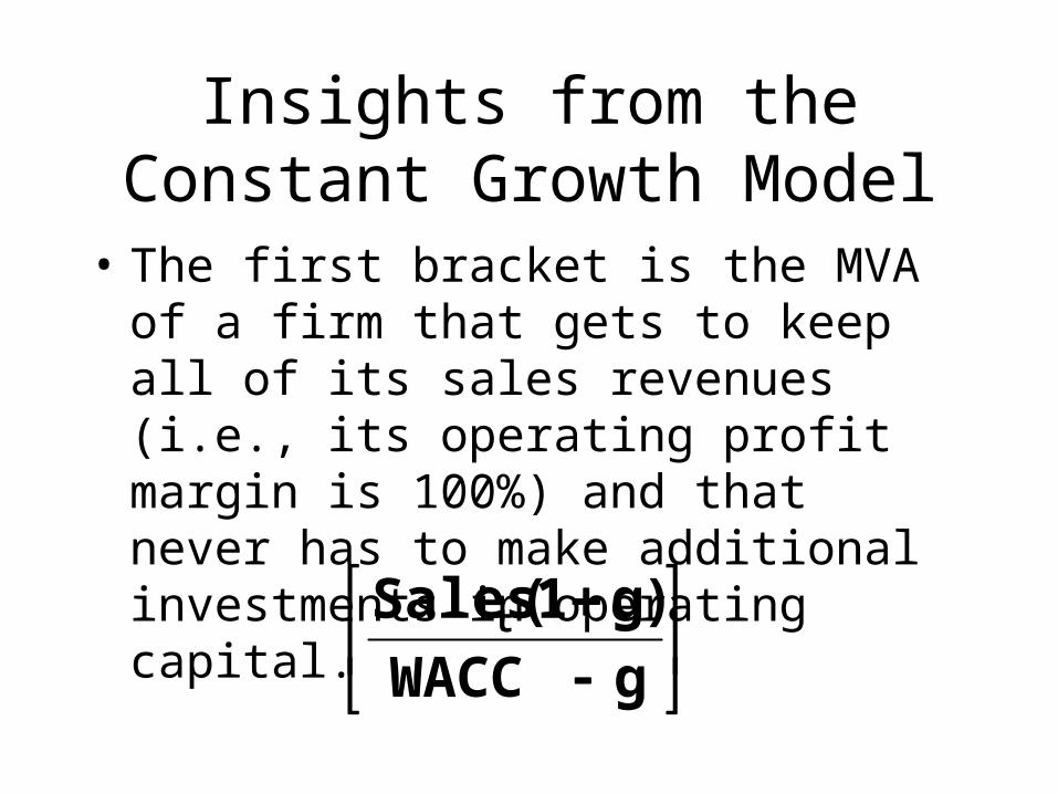
Insights from the Constant Growth Model
• The first bracket is the MVA of a firm that gets to keep all of its sales revenues (i.e., its operating profit margin is 100%) and that never has to make additional investments in operating capital.
gWACC
)g1(Salest

Insights (Cont.)
• The second bracket is the operating profit (as a %) the firm gets to keep, less the return that investors require for having tied up their capital in the firm.
)g1(
CRWACCOP
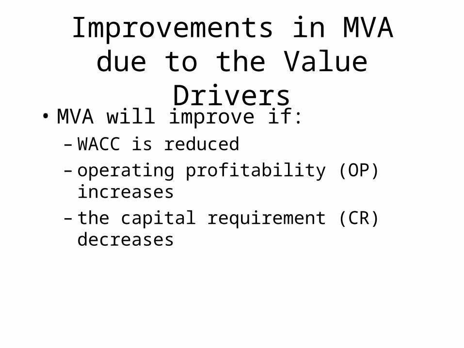
Improvements in MVA due to the Value Drivers
• MVA will improve if:– WACC is reduced– operating profitability (OP) increases– the capital requirement (CR) decreases

The Impact of Growth
• The second term in brackets can be either positive or negative, depending on the relative size of profitability, capital requirements, and required return by investors.
)g1(
CRWACCOP
The Impact of Growth (Cont.)
• If the second term in brackets is negative, then growth decreases MVA. In other words, profits are not enough to offset the return on capital required by investors.
• If the second term in brackets is positive, then growth increases MVA.

Expected Return on Invested Capital (EROIC)
• The expected return on invested capital is the NOPAT expected next period divided by the amount of capital that is currently invested:
t
1tt Capital
NOPATEROIC

MVA in Terms of Expected ROIC
gWACC
WACCEROICCapitalMVA tt
t
If the spread between the expected return, EROICt, and the required return, WACC, is positive, then MVA is positive and growth makes MVA larger. The opposite is true if the spread is negative.
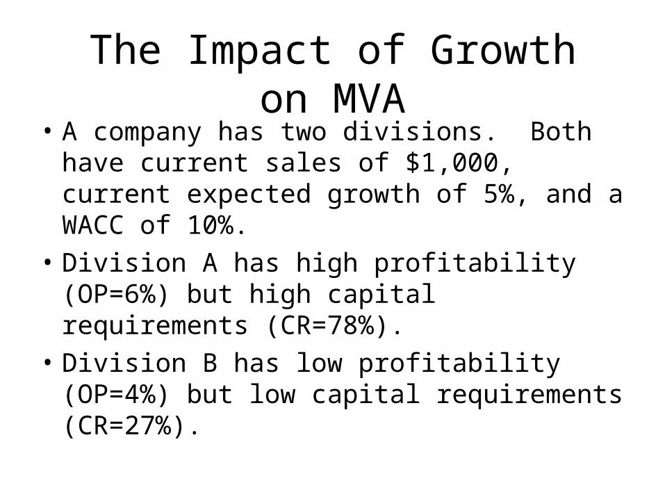
The Impact of Growth on MVA• A company has two divisions. Both have
current sales of $1,000, current expected growth of 5%, and a WACC of 10%.
• Division A has high profitability (OP=6%) but high capital requirements (CR=78%).
• Division B has low profitability (OP=4%) but low capital requirements (CR=27%).
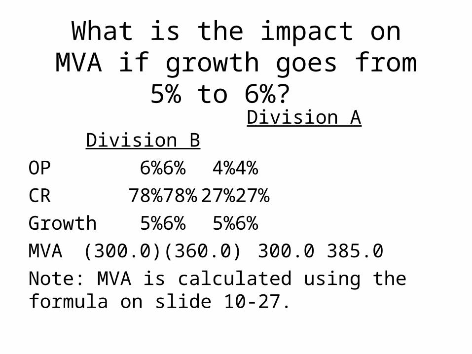
What is the impact on MVA if growth goes from 5% to 6%?
Division A Division B
OP 6% 6% 4% 4%
CR 78% 78% 27% 27%
Growth 5% 6% 5% 6%
MVA (300.0) (360.0) 300.0 385.0
Note: MVA is calculated using the formula on slide 10-27.
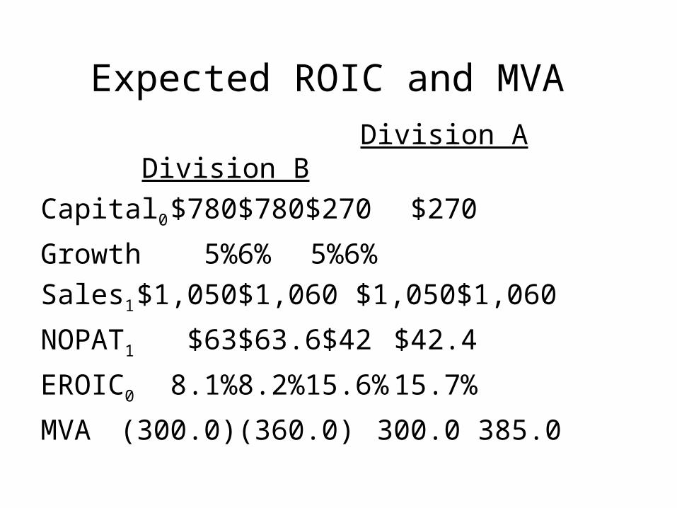
Expected ROIC and MVA
Division A Division B
Capital0 $780 $780 $270 $270
Growth 5% 6% 5% 6%
Sales1 $1,050 $1,060 $1,050 $1,060
NOPAT1 $63 $63.6 $42 $42.4
EROIC0 8.1% 8.2% 15.6% 15.7%
MVA (300.0) (360.0) 300.0 385.0
Analysis of Growth Strategies• The expected ROIC of Division A is less than
the WACC, so the division should postpone growth efforts until it improves EROIC by reducing capital requirements (e.g., reducing inventory) and/or improving profitability.
• The expected ROIC of Division B is greater than the WACC, so the division should continue with its growth plans.
Two Primary Mechanisms of Corporate Governance
• “Stick”– Provisions in the charter that affect takeovers.– Composition of the board of directors.
• “Carrot: Compensation plans.

Entrenched Management
• Occurs when there is little chance that poorly performing managers will be replaced.
• Two causes:– Anti-takeover provisions in the charter– Weak board of directors
How are entrenched managers harmful to shareholders?
• Management consumes perks:– Lavish offices and corporate jets– Excessively large staffs– Memberships at country clubs
• Management accepts projects (or acquisitions) to make firm larger, even if MVA goes down.
Anti-Takeover Provisions
• Targeted share repurchases (i.e., greenmail)
• Shareholder rights provisions (i.e., poison pills)
• Restricted voting rights plans
Board of Directors
• Weak boards have many insiders (i.e., those who also have another position in the company) compared with outsiders.
• Interlocking boards are weaker (CEO of company A sits on board of company B, CEO of B sits on board of A).
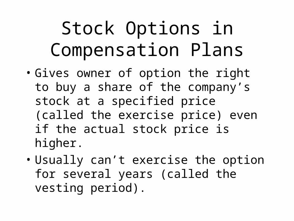
Stock Options in Compensation Plans
• Gives owner of option the right to buy a share of the company’s stock at a specified price (called the exercise price) even if the actual stock price is higher.
• Usually can’t exercise the option for several years (called the vesting period).

Stock Options (Cont.)
• Can’t exercise the option after a certain number of years (called the expiration, or maturity, date).
What types of long-term capital do firms use?
Long-term debt
Preferred stock
Common equity
Capital components are sources of funding that come from investors.
Accounts payable, accruals, and deferred taxes are not sources of funding that come from investors, so they are not included in the calculation of the cost of capital.
We do adjust for these items when calculating the cash flows of a project, but not when calculating the cost of capital.

Should we focus on before-tax or
after-tax capital costs?Tax effects associated with financing can be
incorporated either in capital budgeting cash flows or in cost of capital.
Most firms incorporate tax effects in the cost of capital. Therefore, focus on after-tax costs.
Only cost of debt is affected.

Should we focus on historical (embedded) costs or new
(marginal) costs?
The cost of capital is used primarily to make decisions which involve raising and investing new capital. So, we should focus on marginal costs.

Cost of Debt
• Method 1: Ask an investment banker what the coupon rate would be on new debt.
• Method 2: Find the bond rating for the company and use the yield on other bonds with a similar rating.
• Method 3: Find the yield on the company’s debt, if it has any.
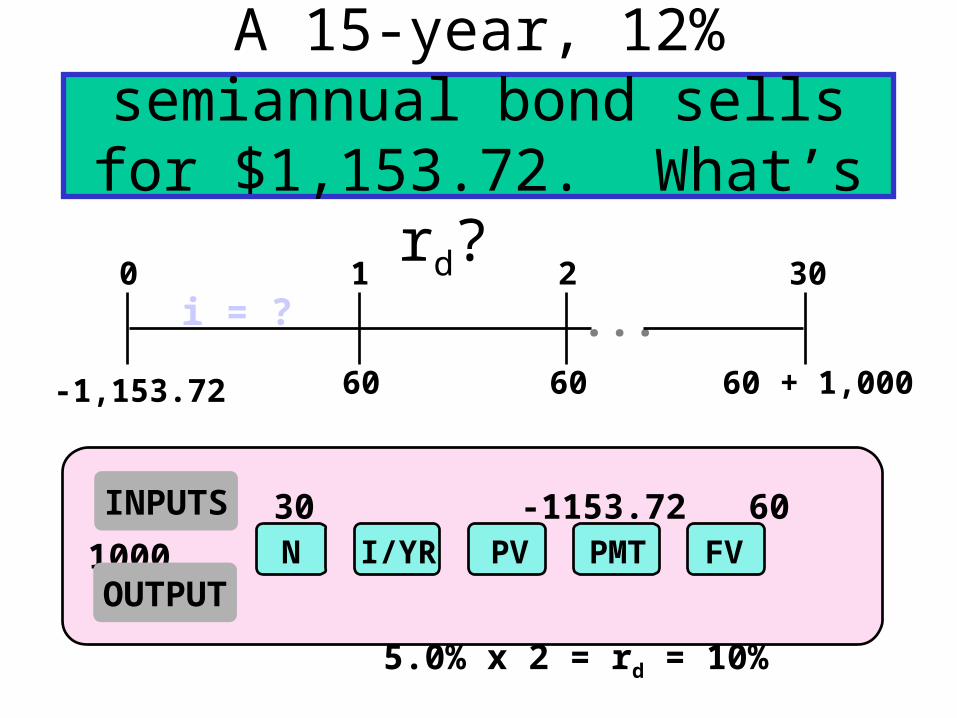
A 15-year, 12% semiannual bond sells for $1,153.72. What’s rd?
60 60 + 1,00060
0 1 2 30i = ?
30 -1153.72 60 1000
5.0% x 2 = rd = 10%
N I/YR PV FVPMT
-1,153.72
...
INPUTS
OUTPUT

Component Cost of Debt
• Interest is tax deductible, so the after tax (AT) cost of debt is:
rd AT = rd BT(1 - T)
= 10%(1 - 0.40) = 6%.
• Use nominal rate.
• Flotation costs small, so ignore.

What’s the cost of preferred stock?
PP = $113.10; 10%Q; Par = $100; F = $2.
%.0.9090.010.111$
10$
00.2$10.113$
100$ 1.0
n
psps P
Dr
Use this formula:
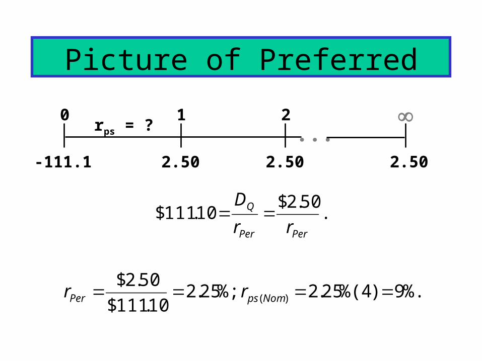
Picture of Preferred
2.50 2.50
0 1 2rps = ?
-111.1
...
2.50
.50.2$
10.111$PerPer
Q
rr
D
%.9)4%(25.2 %;25.210.111$
50.2$)( NompsPer rr

Note:
• Flotation costs for preferred are significant, so are reflected. Use net price.
• Preferred dividends are not deductible, so no tax adjustment. Just rps.
• Nominal rps is used.
Is preferred stock more or less risky to investors than debt?
• More risky; company not required to pay preferred dividend.
• However, firms want to pay preferred dividend. Otherwise, (1) cannot pay common dividend, (2) difficult to raise additional funds, and (3) preferred stockholders may gain control of firm.
Why is yield on preferred lower than rd?
• Corporations own most preferred stock, because 70% of preferred dividends are nontaxable to corporations.
• Therefore, preferred often has a lower B-T yield than the B-T yield on debt.
• The A-T yield to investors and A-T cost to the issuer are higher on preferred than on debt, which is consistent with the higher risk of preferred.

Example:
rps = 9% rd = 10% T = 40%
rps, AT = rps - rps (1 - 0.7)(T)
= 9% - 9%(0.3)(0.4) = 7.92%
rd, AT = 10% - 10%(0.4) = 6.00%
A-T Risk Premium on Preferred = 1.92%

• Directly, by issuing new shares of common stock.
• Indirectly, by reinvesting earnings that are not paid out as dividends (i.e., retaining earnings).
What are the two ways that companies can raise common
equity?
• Earnings can be reinvested or paid out as dividends.
• Investors could buy other securities, earn a return.
• Thus, there is an opportunity cost if earnings are reinvested.
Why is there a cost for reinvested earnings?
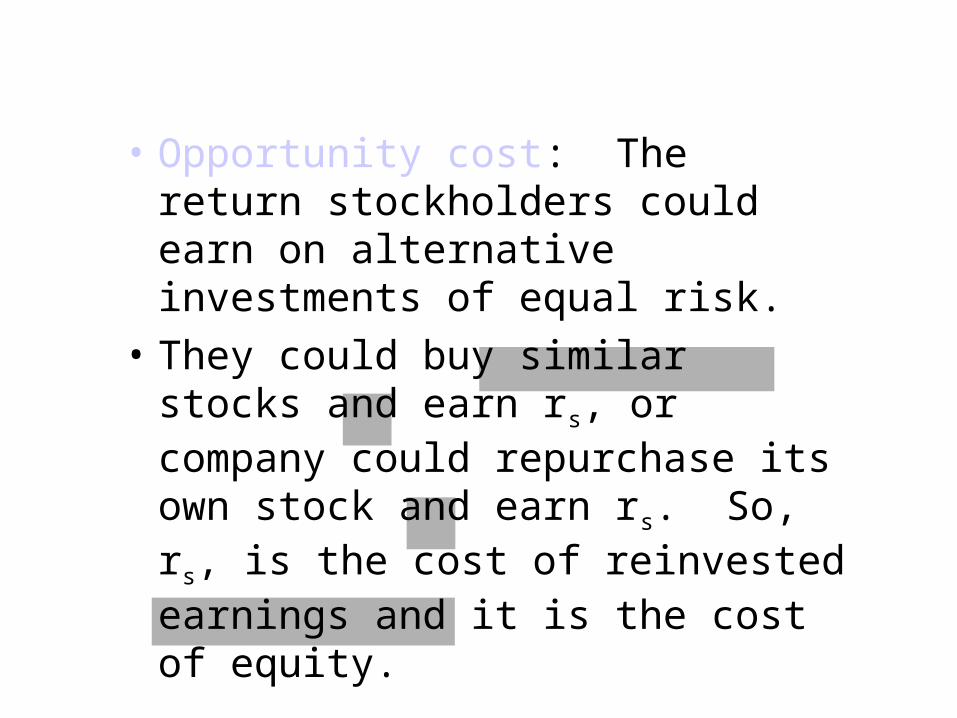
• Opportunity cost: The return stockholders could earn on alternative investments of equal risk.
• They could buy similar stocks and earn rs, or company could repurchase its own stock and earn rs. So, rs, is the cost of reinvested earnings and it is the cost of equity.

Three ways to determine the cost of equity, rs:
1. CAPM: rs = rRF + (rM - rRF)b
= rRF + (RPM)b.
2. DCF: rs = D1/P0 + g.
3. Own-Bond-Yield-Plus-Risk Premium:
rs = rd + RP.
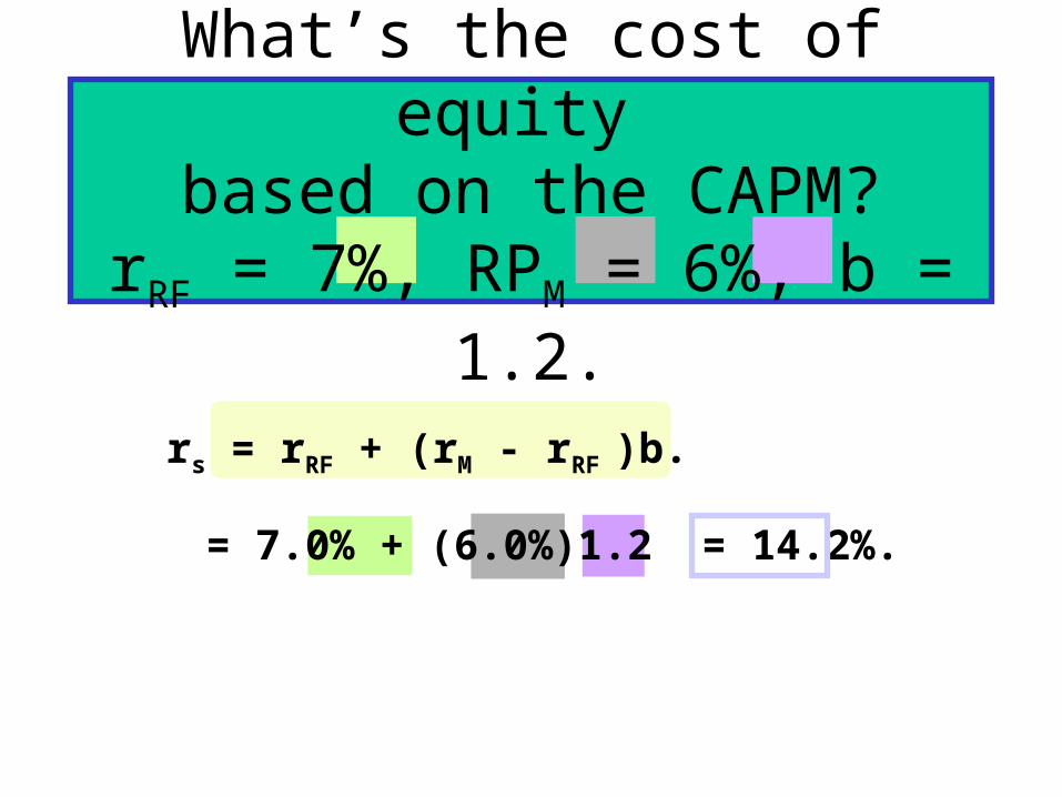
What’s the cost of equity based on the CAPM?
rRF = 7%, RPM = 6%, b = 1.2.
rs = rRF + (rM - rRF )b.
= 7.0% + (6.0%)1.2 = 14.2%.
Issues in Using CAPM
• Most analysts use the rate on a long-term (10 to 20 years) government bond as an estimate of rRF. For a current estimate, go to www.bloomberg.com, select “U.S. Treasuries” from the section on the left under the heading “Market.”
More…
Issues in Using CAPM (Continued)
• Most analysts use a rate of 5% to 6.5% for the market risk premium (RPM)
• Estimates of beta vary, and estimates are “noisy” (they have a wide confidence interval). For an estimate of beta, go to www.bloomberg.com and enter the ticker symbol for STOCK QUOTES.

What’s the DCF cost of equity, rs?Given: D0 = $4.19;P0 = $50; g =
5%.
gP
gDg
P
Drs
0
0
0
1 1
$4. .
$50.
. .
.
19 1050 05
0 088 0 05
13 8%.

Estimating the Growth Rate
• Use the historical growth rate if you believe the future will be like the past.
• Obtain analysts’ estimates: Value Line, Zack’s, Yahoo!.Finance.
• Use the earnings retention model, illustrated on next slide.
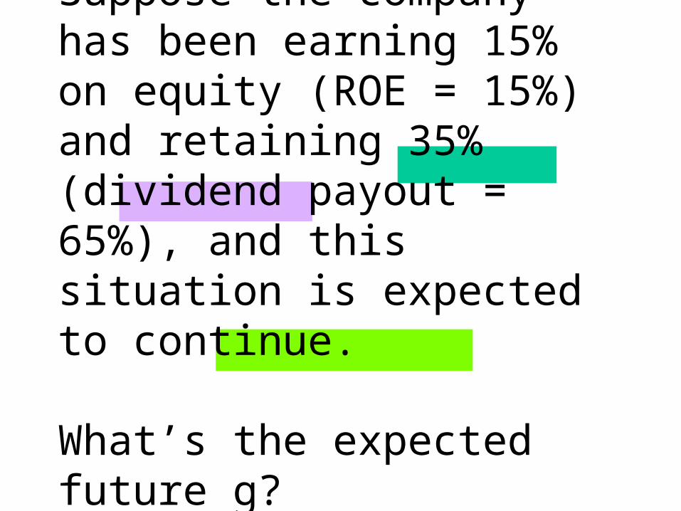
Suppose the company has been earning 15% on equity (ROE = 15%) and retaining 35% (dividend payout = 65%), and this situation is expected to continue.
What’s the expected future g?

Retention growth rate:
g = ROE(Retention rate)
g = 0.35(15%) = 5.25%.
This is close to g = 5% given earlier. Think of bank account paying 15% with retention ratio = 0. What is g of account balance? If retention ratio is 100%, what is g?
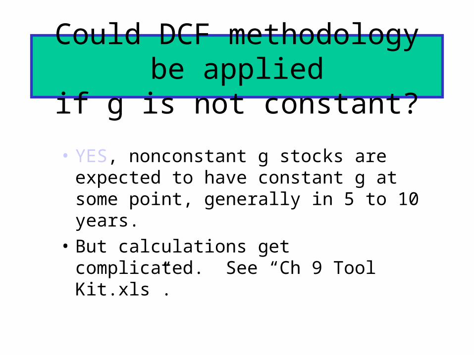
Could DCF methodology be applied
if g is not constant?
• YES, nonconstant g stocks are expected to have constant g at some point, generally in 5 to 10 years.
• But calculations get complicated. See “Ch 9 Tool Kit.xls”.
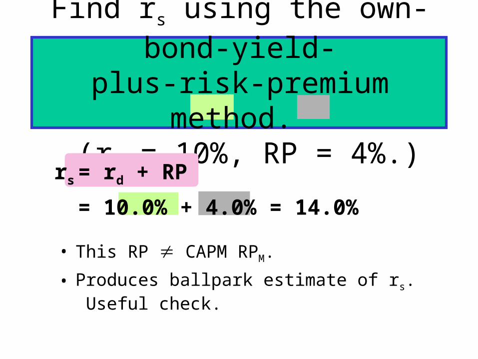
Find rs using the own-bond-yield-plus-risk-premium method.
(rd = 10%, RP = 4%.)
• This RP CAPM RPM.
• Produces ballpark estimate of rs. Useful check.
rs = rd + RP
= 10.0% + 4.0% = 14.0%

What’s a reasonable final estimate
of rs?Method Estimate
CAPM 14.2%
DCF 13.8%
rd + RP 14.0%
Average 14.0%
Determining the Weights for the WACC
• The weights are the percentages of the firm that will be financed by each component.
• If possible, always use the target weights for the percentages of the firm that will be financed with the various types of capital.

Estimating Weights for the Capital Structure
• If you don’t know the targets, it is better to estimate the weights using current market values than current book values.
• If you don’t know the market value of debt, then it is usually reasonable to use the book values of debt, especially if the debt is short-term.
(More...)
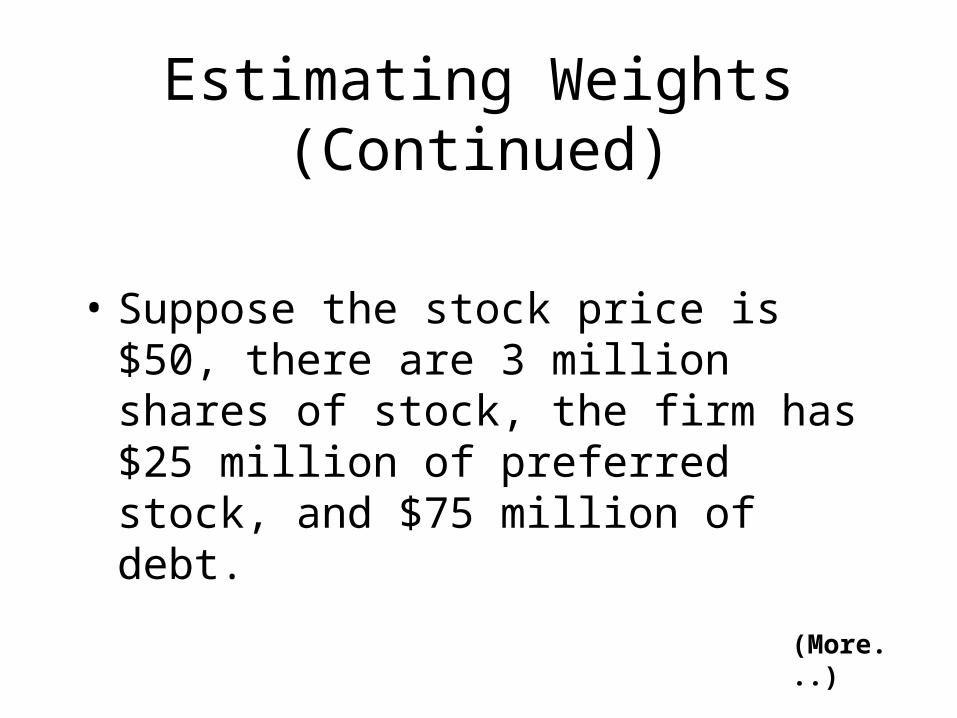
Estimating Weights (Continued)
• Suppose the stock price is $50, there are 3 million shares of stock, the firm has $25 million of preferred stock, and $75 million of debt.
(More...)

• Vce = $50 (3 million) = $150 million.
• Vps = $25 million.
• Vd = $75 million.
• Total value = $150 + $25 + $75 = $250 million.
• wce = $150/$250 = 0.6
• wps = $25/$250 = 0.1
• wd = $75/$250 = 0.3

What’s the WACC?
WACC = wdrd(1 - T) + wpsrps + wcers
= 0.3(10%)(0.6) + 0.1(9%) + 0.6(14%)
= 1.8% + 0.9% + 8.4% = 11.1%.
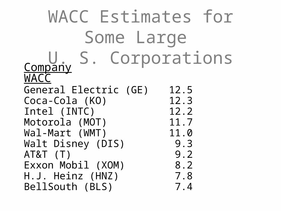
WACC Estimates for Some Large
U. S. CorporationsCompany WACCGeneral Electric (GE) 12.5Coca-Cola (KO) 12.3Intel (INTC) 12.2Motorola (MOT) 11.7Wal-Mart (WMT) 11.0Walt Disney (DIS) 9.3AT&T (T) 9.2Exxon Mobil (XOM) 8.2H.J. Heinz (HNZ) 7.8BellSouth (BLS) 7.4

What factors influence a company’s WACC?
• Market conditions, especially interest rates and tax rates.
• The firm’s capital structure and dividend policy.
• The firm’s investment policy. Firms with riskier projects generally have a higher WACC.
Should the company use the composite WACC as the hurdle
rate for each of its divisions?
• NO! The composite WACC reflects the risk of an average project undertaken by the firm.
• Different divisions may have different risks. The division’s WACC should be adjusted to reflect the division’s risk and capital structure.
• Estimate the cost of capital that the division would have if it were a stand-alone firm.
• This requires estimating the division’s beta, cost of debt, and capital structure.
What procedures are used to determine the risk-adjusted cost
of capital for a particular division?
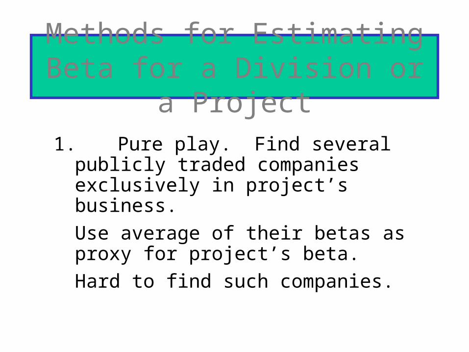
Methods for Estimating Beta for a Division or a Project
1. Pure play. Find several publicly traded companies exclusively in project’s business.
Use average of their betas as proxy for project’s beta.
Hard to find such companies.
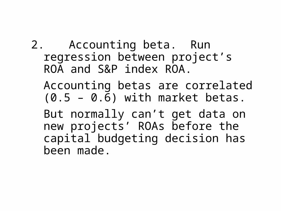
2. Accounting beta. Run regression between project’s ROA and S&P index ROA.
Accounting betas are correlated (0.5 – 0.6) with market betas.
But normally can’t get data on new projects’ ROAs before the capital budgeting decision has been made.
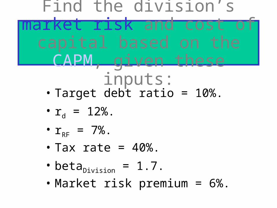
Find the division’s market risk and cost of capital based on the
CAPM, given these inputs:
• Target debt ratio = 10%.
• rd = 12%.
• rRF = 7%.
• Tax rate = 40%.
• betaDivision = 1.7.
• Market risk premium = 6%.
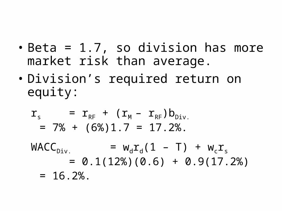
• Beta = 1.7, so division has more market risk than average.
• Division’s required return on equity:
rs = rRF + (rM – rRF)bDiv.
= 7% + (6%)1.7 = 17.2%.
WACCDiv. = wdrd(1 – T) + wcrs
= 0.1(12%)(0.6) + 0.9(17.2%)= 16.2%.
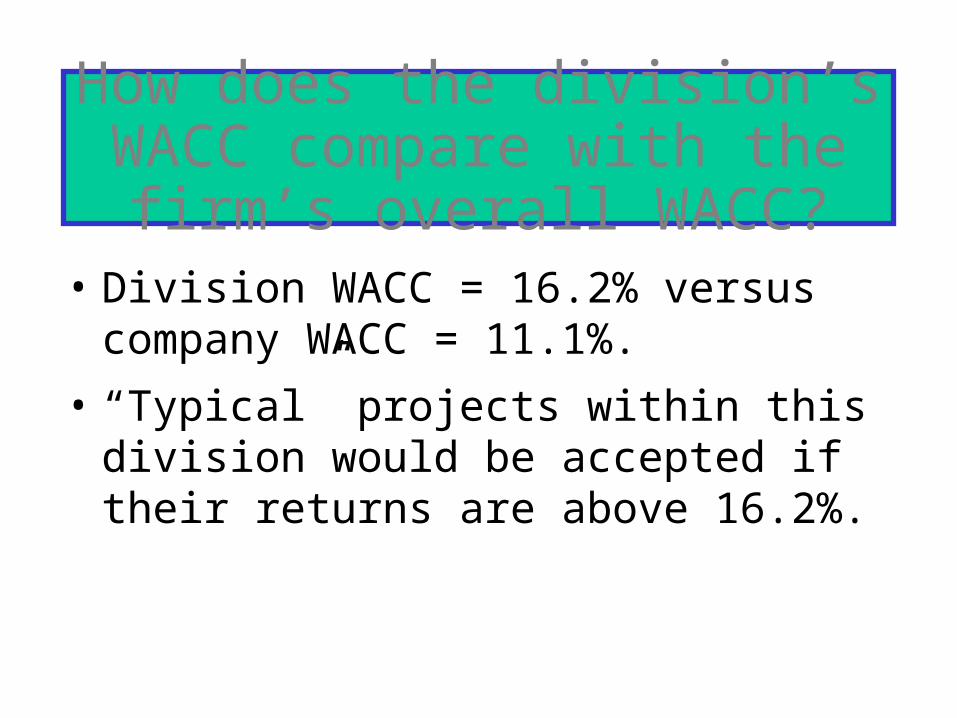
How does the division’s WACC compare with the firm’s overall
WACC?• Division WACC = 16.2% versus company
WACC = 11.1%.
• “Typical” projects within this division would be accepted if their returns are above 16.2%.

Divisional Risk and the Cost of Capital
Rate of Return (%)
WACC
Rejection Region
Acceptance Region
Risk
L
B
A
H WACCH
WACCL
WACCA
0 RiskL RiskA RiskH

What are the three types of project risk?
• Stand-alone risk
• Corporate risk
• Market risk
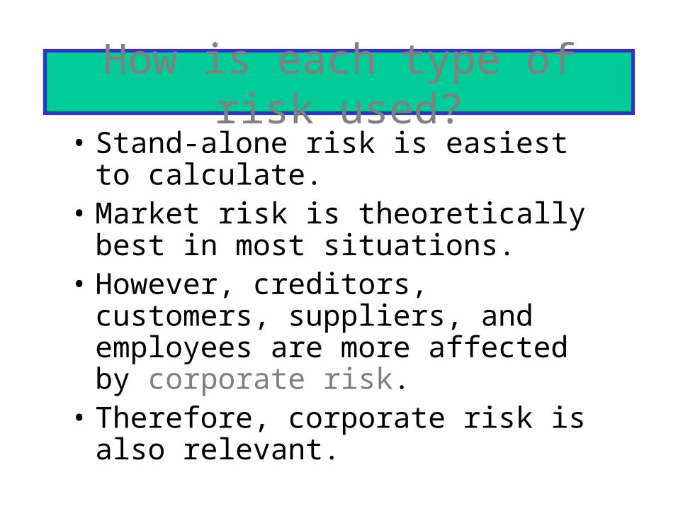
How is each type of risk used?• Stand-alone risk is easiest to calculate.• Market risk is theoretically best in most
situations.• However, creditors, customers, suppliers,
and employees are more affected by corporate risk.
• Therefore, corporate risk is also relevant.

A Project-Specific, Risk-Adjusted
Cost of Capital• Start by calculating a divisional cost of
capital.• Estimate the risk of the project using the
techniques in Chapter 12.• Use judgment to scale up or down the cost
of capital for an individual project relative to the divisional cost of capital.

1. When a company issues new common stock they also have to pay flotation costs to the underwriter.
2. Issuing new common stock may send a negative signal to the capital markets, which may depress stock price.
Why is the cost of internal equity from reinvested earnings cheaper
than the cost of issuing new common stock?
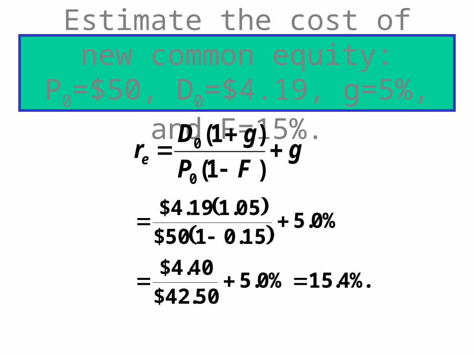
Estimate the cost of new common equity: P0=$50,
D0=$4.19, g=5%, and F=15%.g
FP
gDre
)1(
)1(
0
0
%.4.15%0.550.42$
40.4$
%0.515.0150$05.119.4$
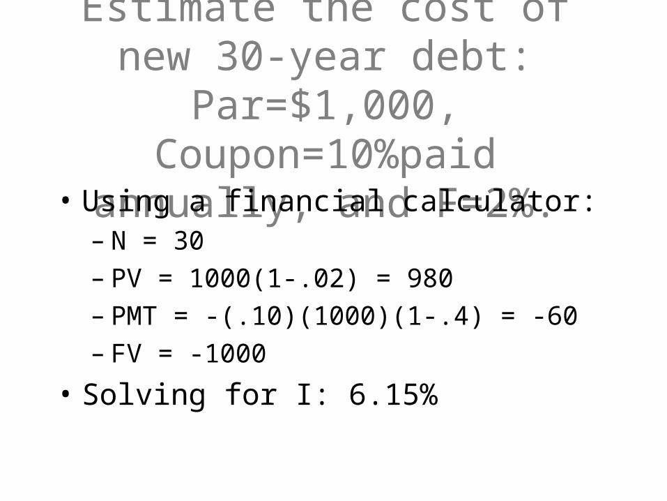
Estimate the cost of new 30-year debt: Par=$1,000,
Coupon=10%paid annually, and F=2%.
• Using a financial calculator:– N = 30– PV = 1000(1-.02) = 980– PMT = -(.10)(1000)(1-.4) = -60– FV = -1000
• Solving for I: 6.15%

Comments about flotation costs:
• Flotation costs depend on the risk of the firm and the type of capital being raised.
• The flotation costs are highest for common equity. However, since most firms issue equity infrequently, the per-project cost is fairly small.
• We will frequently ignore flotation costs when calculating the WACC.
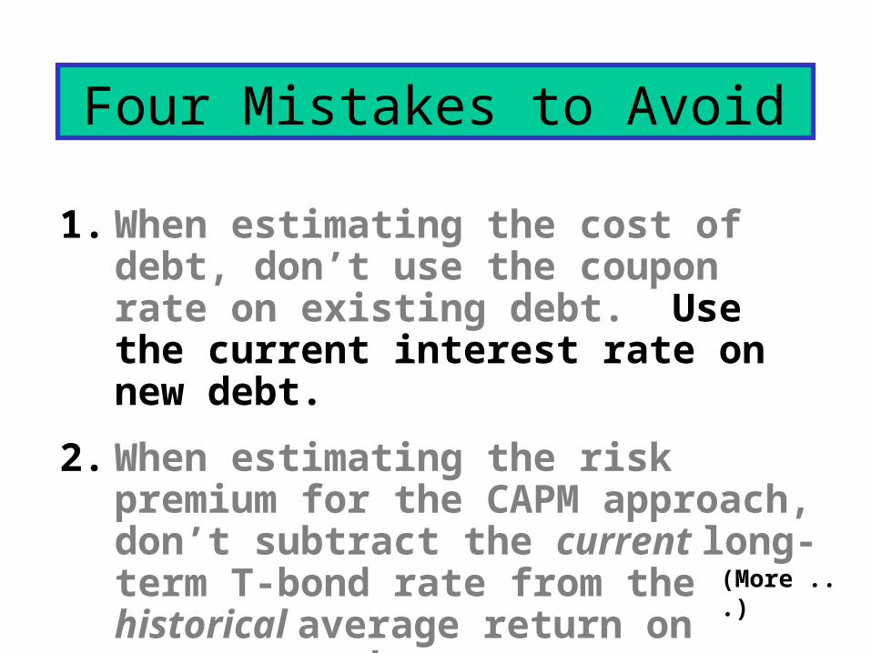
Four Mistakes to Avoid
1. When estimating the cost of debt, don’t use the coupon rate on existing debt. Use the current interest rate on new debt.
2. When estimating the risk premium for the CAPM approach, don’t subtract the current long-term T-bond rate from the historical average return on common stocks. (More ...)

For example, if the historical rM has been about 12.7% and inflation drives the current rRF up to 10%, the current market risk premium is not 12.7% - 10% = 2.7%!
(More ...)

3. Don’t use book weights to estimate the weights for the capital structure.
Use the target capital structure to determine the weights.
If you don’t know the target weights, then use the current market value of equity, and never the book value of equity.
If you don’t know the market value of debt, then the book value of debt often is a reasonable approximation, especially for short-term debt.
(More...)

4. Always remember that capital components are sources of funding that come from investors.
Accounts payable, accruals, and deferred taxes are not sources of funding that come from investors, so they are not included in the calculation of the WACC.
We do adjust for these items when calculating the cash flows of the project, but not when calculating the WACC.
Financial Planning and Pro Forma Statements
• Three important uses:– Forecast the amount of external financing that
will be required– Evaluate the impact that changes in the
operating plan have on the value of the firm– Set appropriate targets for compensation plans
Steps in Financial Forecasting
• Forecast sales
• Project the assets needed to support sales
• Project internally generated funds
• Project outside funds needed
• Decide how to raise funds
• See effects of plan on ratios and stock price
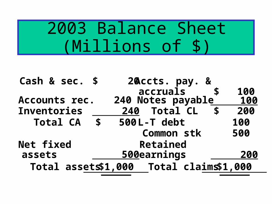
2003 Balance Sheet(Millions of $)
Cash & sec. $ 20 Accts. pay. &accruals $ 100
Accounts rec. 240 Notes payable 100Inventories 240 Total CL $ 200 Total CA $ 500 L-T debt 100
Common stk 500Net fixedassets
Retainedearnings 200
Total assets $1,000 Total claims $1,000 500
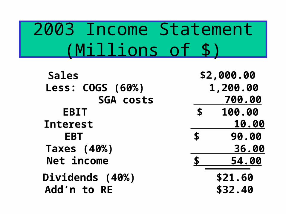
2003 Income Statement(Millions of $)
Sales $2,000.00Less: COGS (60%) 1,200.00 SGA costs 700.00 EBIT $ 100.00Interest 10.00 EBT $ 90.00Taxes (40%) 36.00Net income $ 54.00
Dividends (40%) $21.60Add’n to RE $32.40
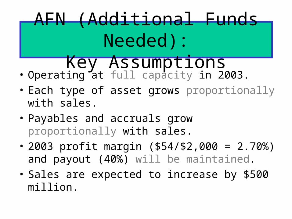
AFN (Additional Funds Needed):Key Assumptions
• Operating at full capacity in 2003.
• Each type of asset grows proportionally with sales.
• Payables and accruals grow proportionally with sales.
• 2003 profit margin ($54/$2,000 = 2.70%) and payout (40%) will be maintained.
• Sales are expected to increase by $500 million.
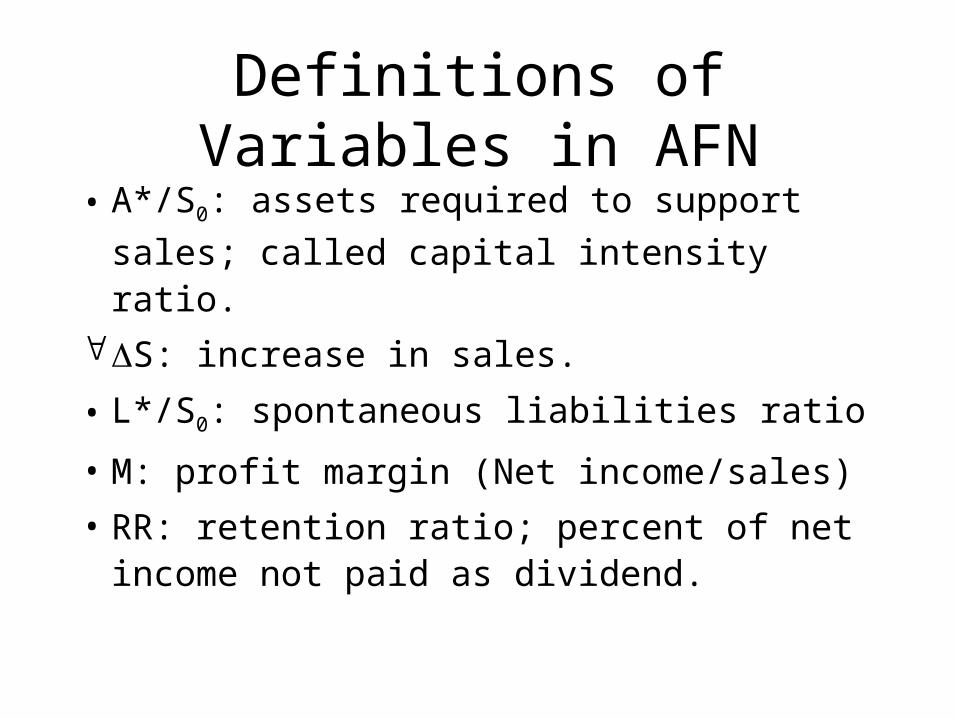
Definitions of Variables in AFN
• A*/S0: assets required to support sales;
called capital intensity ratio.
S: increase in sales.
• L*/S0: spontaneous liabilities ratio
• M: profit margin (Net income/sales)
• RR: retention ratio; percent of net income not paid as dividend.

Assets
Sales0
1,000
2,000
1,250
2,500
A*/S0 = $1,000/$2,000 = 0.5 = $1,250/$2,500.
Assets =(A*/S0)Sales= 0.5($500)= $250.
Assets = 0.5 sales
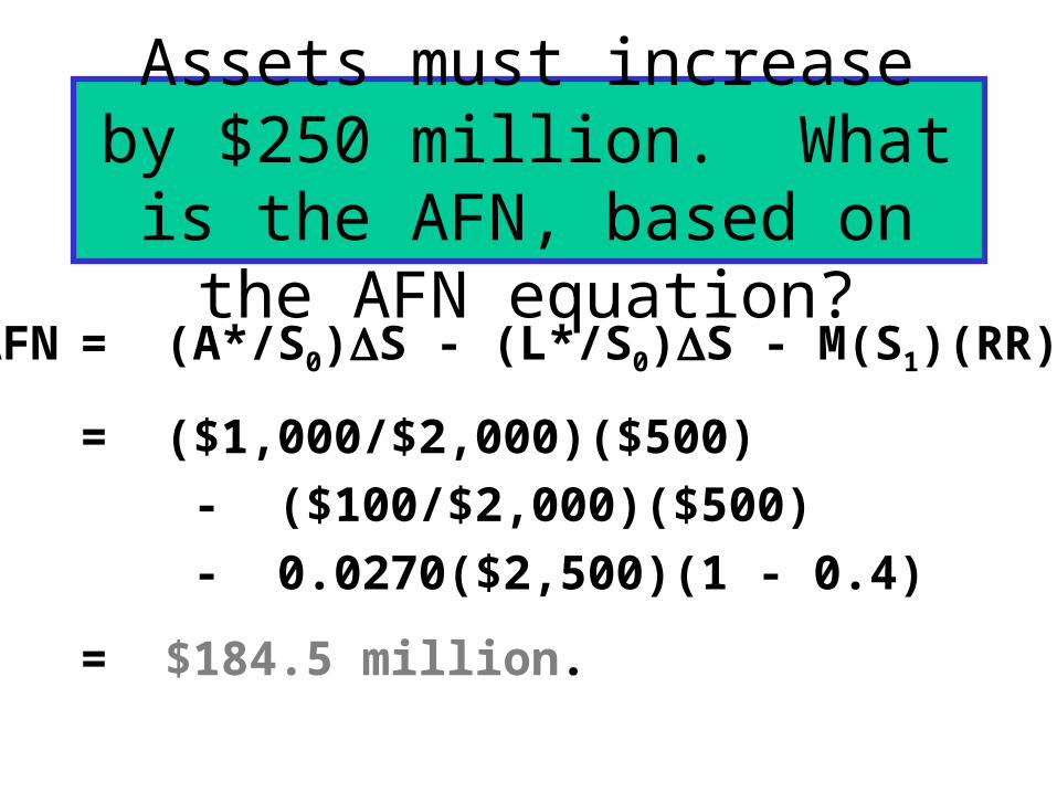
Assets must increase by $250 million. What is the AFN, based
on the AFN equation?AFN = (A*/S0)S - (L*/S0)S - M(S1)(RR)
= ($1,000/$2,000)($500)
- ($100/$2,000)($500)
- 0.0270($2,500)(1 - 0.4)
= $184.5 million.

How would increases in these items affect the AFN?
• Higher sales:– Increases asset requirements, increases AFN.
• Higher dividend payout ratio:– Reduces funds available internally, increases
AFN.
(More…)

• Higher profit margin:– Increases funds available internally, decreases
AFN.
• Higher capital intensity ratio, A*/S0:
– Increases asset requirements, increases AFN.
• Pay suppliers sooner:– Decreases spontaneous liabilities, increases
AFN.

Projecting Pro Forma Statements with the Percent of Sales Method• Project sales based on forecasted growth
rate in sales
• Forecast some items as a percent of the forecasted sales– Costs– Cash– Accounts receivable
(More...)

• Items as percent of sales (Continued...)
– Inventories
– Net fixed assets
– Accounts payable and accruals
• Choose other items– Debt
– Dividend policy (which determines retained earnings)
– Common stock

Sources of Financing Needed to Support Asset Requirements
• Given the previous assumptions and choices, we can estimate:– Required assets to support sales– Specified sources of financing
• Additional funds needed (AFN) is:– Required assets minus specified sources of
financing
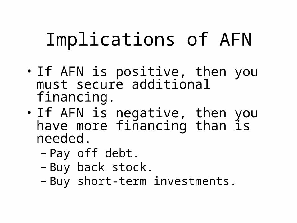
Implications of AFN
• If AFN is positive, then you must secure additional financing.
• If AFN is negative, then you have more financing than is needed.– Pay off debt.– Buy back stock.– Buy short-term investments.

How to Forecast Interest Expense• Interest expense is actually based on the
daily balance of debt during the year.• There are three ways to approximate
interest expense. Base it on: – Debt at end of year– Debt at beginning of year– Average of beginning and ending debt
More…

Basing Interest Expense on Debt at End of Year
• Will over-estimate interest expense if debt is added throughout the year instead of all on January 1.
• Causes circularity called financial feedback: more debt causes more interest, which reduces net income, which reduces retained earnings, which causes more debt, etc.
More…

Basing Interest Expense on Debt at Beginning of Year
• Will under-estimate interest expense if debt is added throughout the year instead of all on December 31.
• But doesn’t cause problem of circularity.
More…
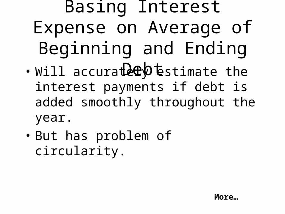
Basing Interest Expense on Average of Beginning and
Ending Debt• Will accurately estimate the interest
payments if debt is added smoothly throughout the year.
• But has problem of circularity.
More…

A Solution that Balances Accuracy and Complexity
• Base interest expense on beginning debt, but use a slightly higher interest rate.– Easy to implement– Reasonably accurate
• See Ch 8 Mini Case Feedback.xls for an example basing interest expense on average debt.

Percent of Sales: Inputs
COGS/Sales 60% 60%
SGA/Sales 35% 35%
Cash/Sales 1% 1%
Acct. rec./Sales 12% 12%
Inv./Sales 12% 12%
Net FA/Sales 25% 25%
AP & accr./Sales 5% 5%
2003 2004Actual Proj.

Other Inputs
Percent growth in sales 25%
Growth factor in sales (g) 1.25
Interest rate on debt 10%
Tax rate 40%
Dividend payout rate 40%

2004 Forecasted Income Statement
2003 Factor2004
1st PassSales $2,000 g=1.25 $2,500.0
Less: COGS Pct=60% 1,500.0 SGA Pct=35% 875.0 EBIT $125.0Interest 0.1(Debt03) 20.0 EBT $105.0Taxes (40%) 42.0Net. income $63.0
Div. (40%) $25.2Add. to RE $37.8

2004 Balance Sheet (Assets)Forecasted assets are a percent of forecasted sales.
Factor 2004
Cash
Pct= 1% $25.0Accts. rec. Pct=12% 300.0
Pct=12% 300.0
Total CA
$625.0Net FA Pct=25% 625.0Total assets $1,250.0
2004 Sales = $2,500
Inventories
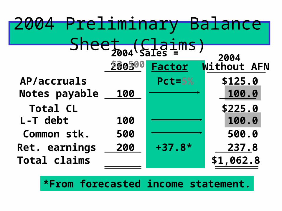
2004 Preliminary Balance Sheet (Claims)
*From forecasted income statement.
2003 Factor Without AFN
AP/accruals Pct=5% $125.0Notes payable 100 100.0
Total CL $225.0L-T debt 100 100.0Common stk. 500 500.0Ret. earnings 200 +37.8* 237.8Total claims $1,062.8
20042004 Sales = $2,500

• Required assets = $1,250.0
• Specified sources of fin. = $1,062.8
• Forecast AFN = $ 187.2
What are the additional funds needed (AFN)?
NWC must have the assets to make forecasted sales, and so it needs an equal amount of financing. So, we must secure another $187.2 of financing.

Assumptions about How AFN Will
Be Raised
• No new common stock will be issued.
• Any external funds needed will be raised as debt, 50% notes payable, and 50% L-T debt.
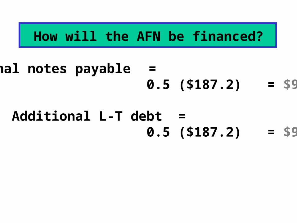
How will the AFN be financed?
Additional notes payable = 0.5 ($187.2) = $93.6.
Additional L-T debt = 0.5 ($187.2) = $93.6.
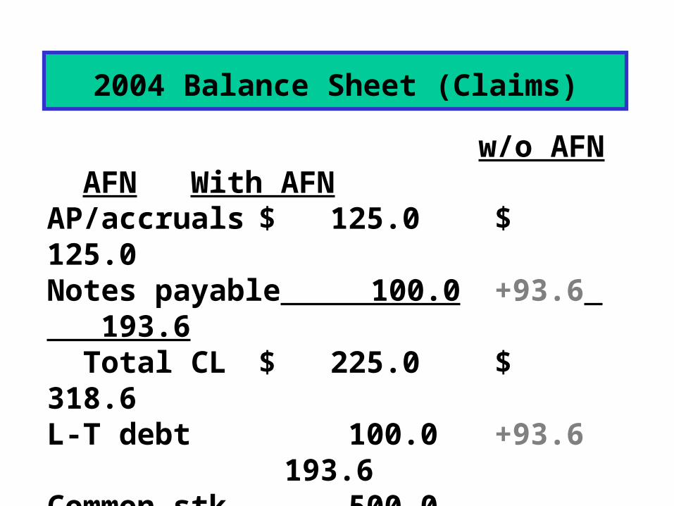
2004 Balance Sheet (Claims)
w/o AFN AFN With AFNAP/accruals $ 125.0 $ 125.0 Notes payable 100.0 +93.6 193.6 Total CL $ 225.0 $ 318.6 L-T debt 100.0 +93.6 193.6 Common stk. 500.0 500.0Ret. earnings 237.8 237.8 Total claims $1,071.0 $1,250.0

Equation method assumes a constant profit margin.
Pro forma method is more flexible. More important, it allows different items to grow at different rates.
Equation AFN = $184.5 vs.
Pro Forma AFN = $187.2.Why are they different?
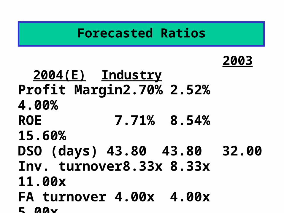
Forecasted Ratios
2003 2004(E) IndustryProfit Margin 2.70% 2.52% 4.00%ROE 7.71% 8.54% 15.60%DSO (days) 43.80 43.80 32.00Inv. turnover 8.33x 8.33x 11.00xFA turnover 4.00x 4.00x 5.00xDebt ratio 30.00% 40.98% 36.00%TIE 10.00x 6.25x 9.40xCurrent ratio 2.50x 1.96x 3.00x
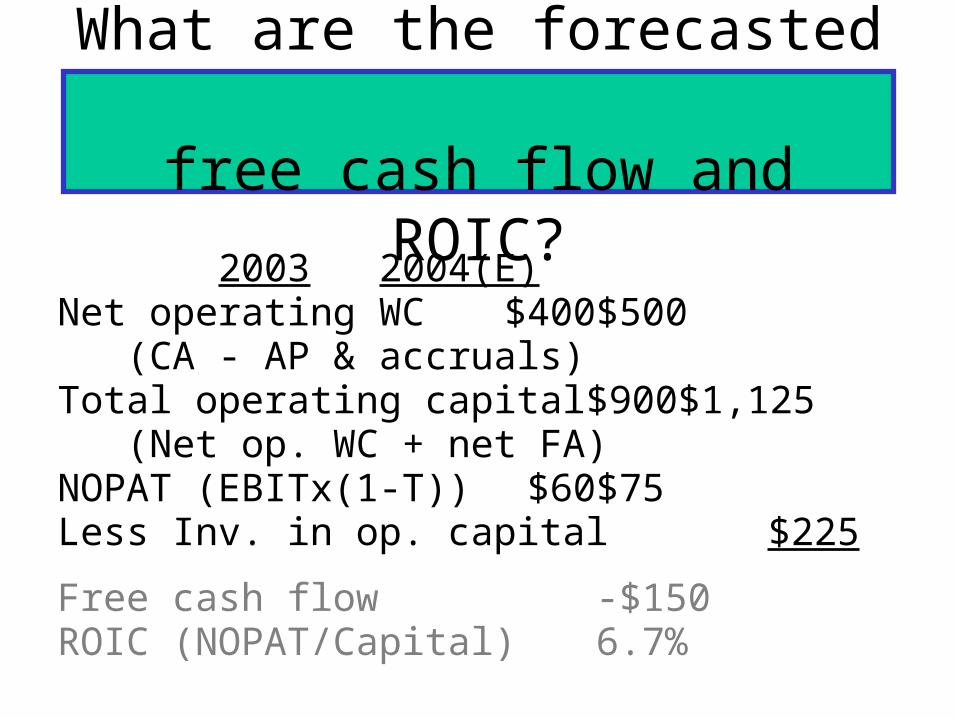
What are the forecasted free cash flow and ROIC?
2003 2004(E)Net operating WC $400 $500 (CA - AP & accruals)Total operating capital $900 $1,125 (Net op. WC + net FA)NOPAT (EBITx(1-T)) $60 $75 Less Inv. in op. capital $225
Free cash flow -$150ROIC (NOPAT/Capital) 6.7%
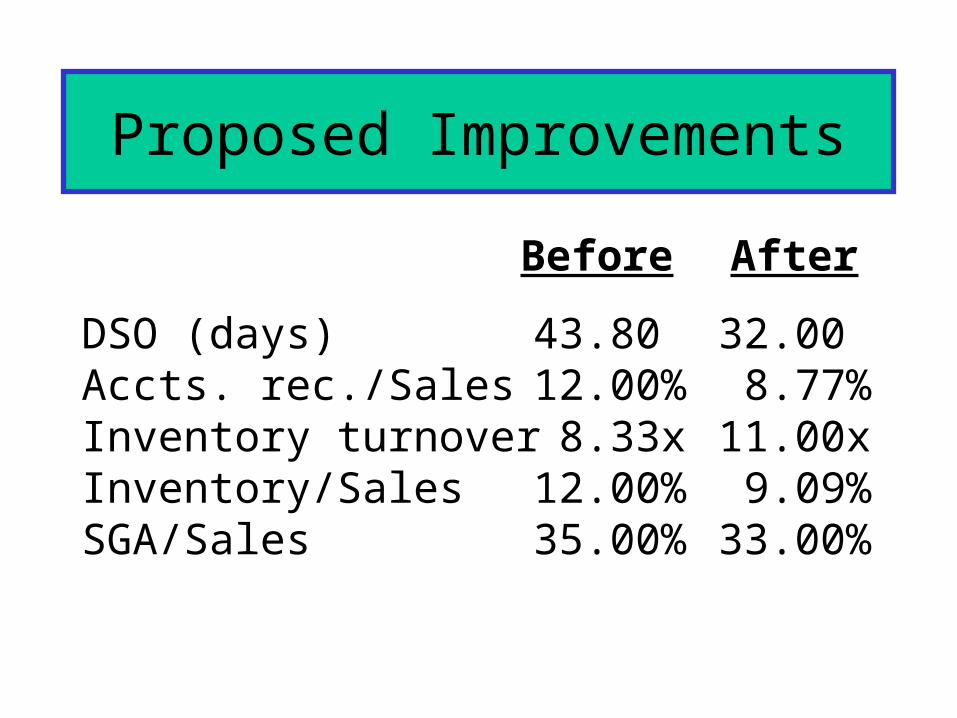
Proposed Improvements
DSO (days) 43.80 32.00Accts. rec./Sales 12.00% 8.77%Inventory turnover 8.33x 11.00xInventory/Sales 12.00% 9.09%SGA/Sales 35.00% 33.00%
Before After
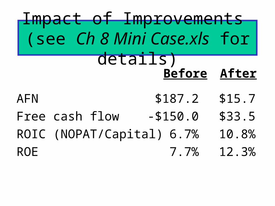
Impact of Improvements (see Ch 8 Mini Case.xls for
details)
AFN $187.2 $15.7
Free cash flow -$150.0 $33.5
ROIC (NOPAT/Capital) 6.7% 10.8%
ROE 7.7% 12.3%
Before After

Suppose in 2003 fixed assets had been operated at only 75% of
capacity.
With the existing fixed assets, sales could be $2,667. Since sales are forecasted at only $2,500, no new fixed assets are needed.
Capacity sales =Actual sales
% of capacity
= = $2,667.$2,000
0.75
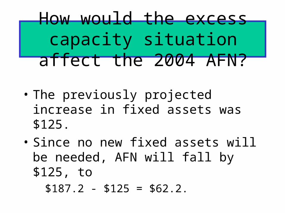
How would the excess capacity situation affect the 2004 AFN?
• The previously projected increase in fixed assets was $125.
• Since no new fixed assets will be needed, AFN will fall by $125, to
$187.2 - $125 = $62.2.

Assets
Sales0
1,1001,000
2,000 2,500
Declining A/S Ratio
$1,000/$2,000 = 0.5; $1,100/$2,500 = 0.44. Declining ratio shows economies of scale. Going from S = $0 to S = $2,000 requires $1,000 of assets. Next $500 of sales requires only $100 of assets.
BaseStock
Economies of Scale
Assets
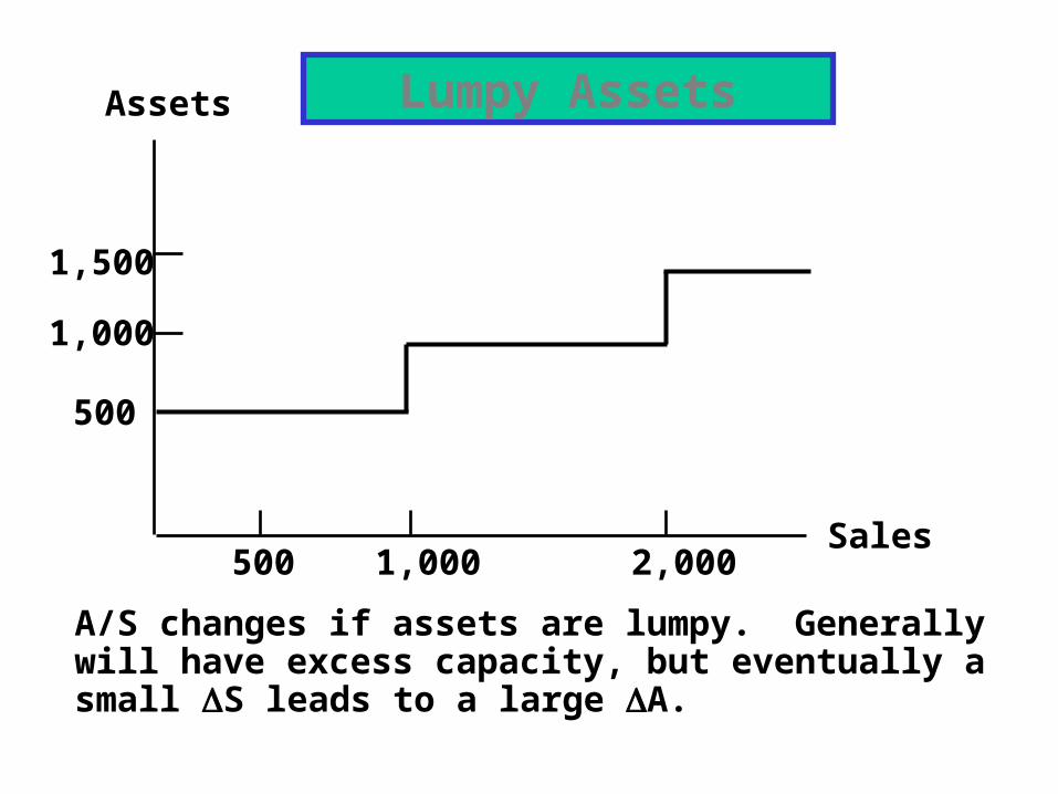
Sales1,000 2,000500
A/S changes if assets are lumpy. Generally will have excess capacity, but eventually a small S leads to a large A.
500
1,000
1,500
Lumpy Assets

Summary: How different factors affect
the AFN forecast.• Excess capacity: lowers AFN.
• Economies of scale: leads to less-than-proportional asset increases.
• Lumpy assets: leads to large periodic AFN requirements, recurring excess capacity.
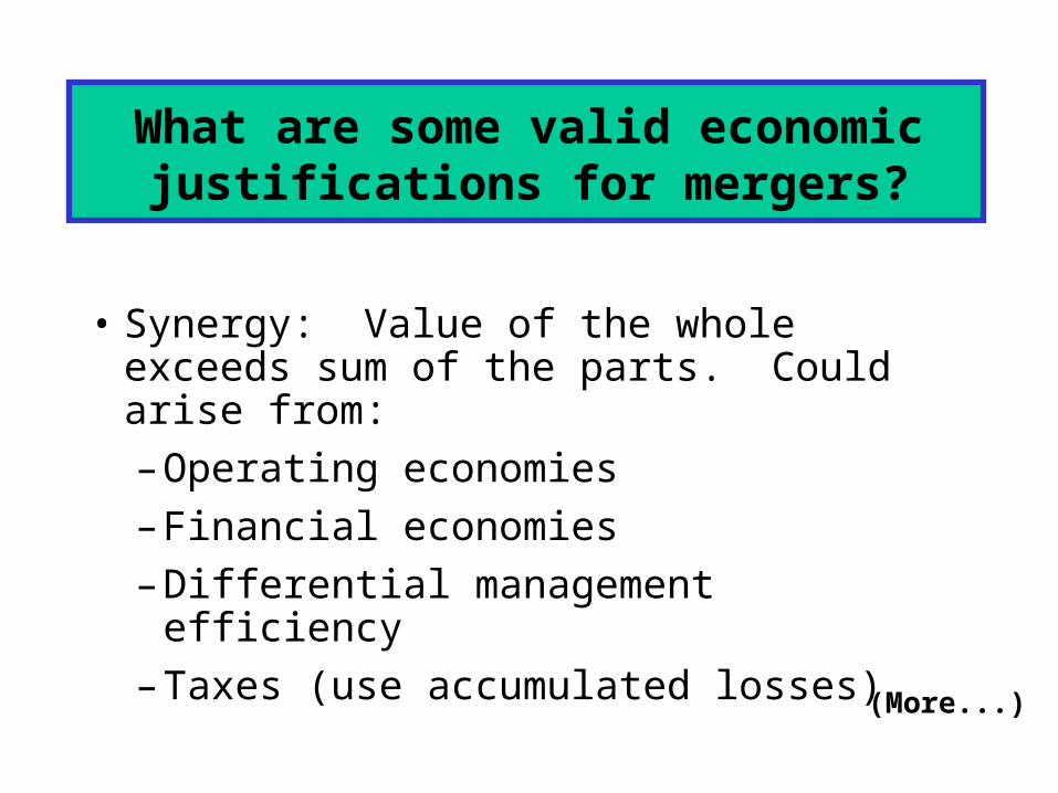
• Synergy: Value of the whole exceeds sum of the parts. Could arise from:
– Operating economies
– Financial economies
– Differential management efficiency
– Taxes (use accumulated losses)
What are some valid economicjustifications for mergers?
(More...)
• Break-up value: Assets would be more valuable if broken up and sold to other companies.
• Diversification
• Purchase of assets at below replacement cost
• Acquire other firms to increase size, thus making it more difficult to be acquired
What are some questionablereasons for mergers?

• Friendly merger:
– The merger is supported by the managements of both firms.
Differentiate between hostile and friendly mergers
(More...)
• Hostile merger:
– Target firm’s management resists the merger.
– Acquirer must go directly to the target firm’s stockholders, try to get 51% to tender their shares.
– Often, mergers that start out hostile end up as friendly, when offer price is raised.

• Access to new markets and technologies• Multiple parties share risks and expenses• Rivals can often work together
harmoniously• Antitrust laws can shelter cooperative
R&D activities
Reasons why alliances can make more sense than acquisitions

Reason for APV
• Often in a merger the capital structure changes rapidly over the first several years.
• This causes the WACC to change from year to year.
• It is hard to incorporate year-to-year changes in WACC in the corporate valuation model.
The APV Model
Value of firm if it had no debt+ Value of tax savings due to debt= Value of operations
First term is called the unlevered value of the firm. The second term is called the value of the interest tax shield.
(More...)

APV Model
Unlevered value of firm = PV of FCFs discounted at unlevered cost of equity, rsU.
Value of interest tax shield = PV of interest tax savings at unlevered cost of equity. Interest tax savings =
Interest(tax rate) = TSt .
Note to APV
• APV is the best model to use when the capital structure is changing.
• The Corporate Valuation model is easier than APV to use when the capital structure is constant—such as at the horizon.

Steps in APV Valuation
1. Project FCFt ,TSt , horizon growth rate, and horizon capital structure.
2. Calculate the unlevered cost of equity, rsU.3. Calculate WACC at horizon.4. Calculate horizon value using constant growth
corporate valuation model.
5. Calculate Vops as PV of FCFt, TSt and horizon value, all discounted at rsU.

Net sales $60.0 $90.0 $112.5 $127.5Cost of goods sold (60%) 36.0 54.0 67.5 76.5Selling/admin. expenses 4.5 6.0 7.5 9.0EBIT 19.5 30.0 37.5 42.0Taxes on EBIT (40%) 7.8 12.0 15.0 16.8NOPAT 11.7 18.0 22.5 25.2Net Retentions 0.0 7.5 6.0 4.5Free Cash Flow 11.7 10.5 16.5 20.7
APV Valuation Analysis (In Millions)
2004 2005 2006 2007 Free Cash Flows after Merger Occurs
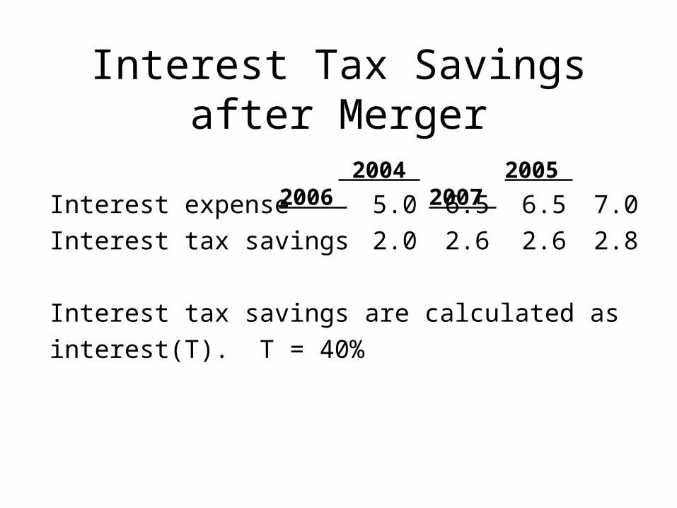
Interest Tax Savings after Merger
Interest expense 5.0 6.5 6.5 7.0
Interest tax savings 2.0 2.6 2.6 2.8
Interest tax savings are calculated as
interest(T). T = 40%
2004 2005 2006 2007
What are the net retentions?
• Recall that firms must reinvest in order to replace worn out assets and grow.
• Net retentions = gross retentions – depreciation.

• After acquisition, the free cash flows belong to the remaining debtholders in the target and the various investors in the acquiring firm: their debtholders, stockholders, and others such as preferred stockholders.
• These cash flows can be redeployed within the acquiring firm.
Conceptually, what is the appropriate discount rate to apply to the
target’s cash flows?
(More...)

• Free cash flow is the cash flow that would occur if the firm had no debt, so it should be discounted at the unlevered cost of equity.
• The interest tax shields are also discounted at the unlevered cost of equity.
Note: Comparison of APV with Corporate Valuation Model
• APV discounts FCF at rsU and adds in present value of the tax shields—the value of the tax savings are incorporated explicitly.
• Corp. Val. Model discounts FCF at WACC, which has a (1-T) factor to account for the value of the tax shield.
• Both models give same answer IF carefully done. BUT it is difficult to apply the Corp. Val. Model when WACC is changing from year-to-year.
Discount rate for Horizon Value
• At the horizon the capital structure is constant, so the corporate valuation model can be used, so discount FCFs at WACC.
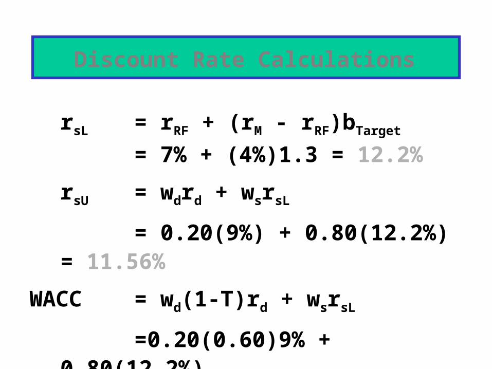
Discount Rate Calculations
rsL = rRF + (rM - rRF)bTarget
= 7% + (4%)1.3 = 12.2%
rsU = wdrd + wsrsL
= 0.20(9%) + 0.80(12.2%) = 11.56%
WACC = wd(1-T)rd + wsrsL
=0.20(0.60)9% + 0.80(12.2%)
= 10.84%

Horizon value =
=
= $453.3 million.
Horizon, or Continuing, Value
g WACC
g))(1(FCF2007
06.01084.0
)06.1(7.20$
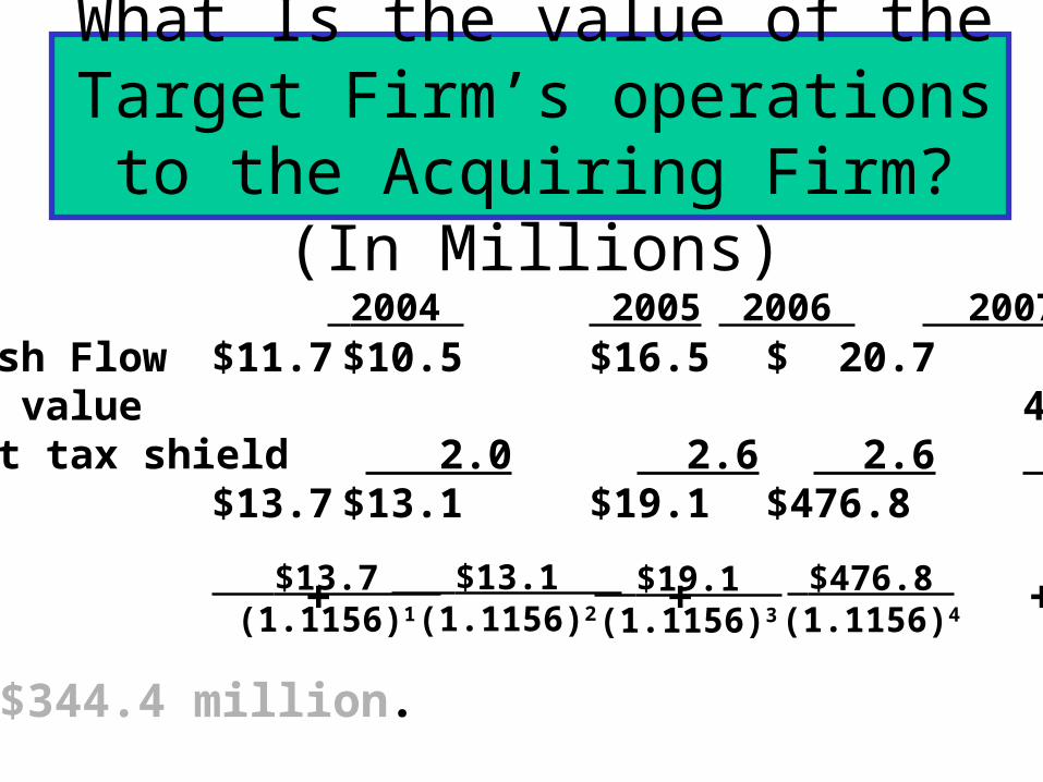
What Is the value of the Target Firm’s operations to the Acquiring
Firm? (In Millions)
2004 2005 2006 2007 Free Cash Flow $11.7 $10.5 $16.5 $ 20.7Horizon value 453.3Interest tax shield 2.0 2.6 2.6 2.8Total $13.7 $13.1 $19.1 $476.8
VOps = + + +
= $344.4 million.
$13.7 (1.1156)1
$13.1 (1.1156)2
$19.1 (1.1156)3
$476.8 (1.1156)4

What is the value of the Target’s equity?
• The Target has $55 million in debt.
• Vops – debt = equity
• 344.4 million – 55 million = $289.4 million = equity value of target to the acquirer.
• No. The cash flow estimates would be different, both due to forecasting inaccuracies and to differential synergies.
• Further, a different beta estimate, financing mix, or tax rate would change the discount rate.
Would another potential acquirer obtain the same value?
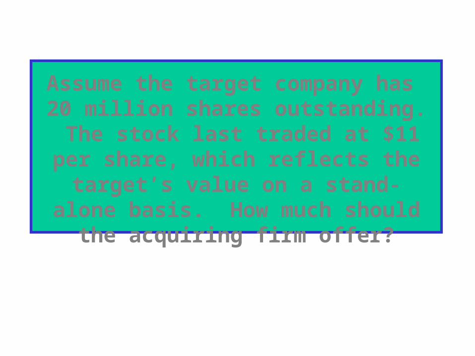
Assume the target company has 20 million shares outstanding. The stock last traded at $11 per share,
which reflects the target’s value on a stand-alone basis. How much should
the acquiring firm offer?

Estimate of target’s value = $289.4 million
Target’s current value = $220.0million
Merger premium = $ 69.4 million
Presumably, the target’s value is increased by $69.4 million due to merger synergies, although realizing such synergies has been problematic in many mergers.
(More...)

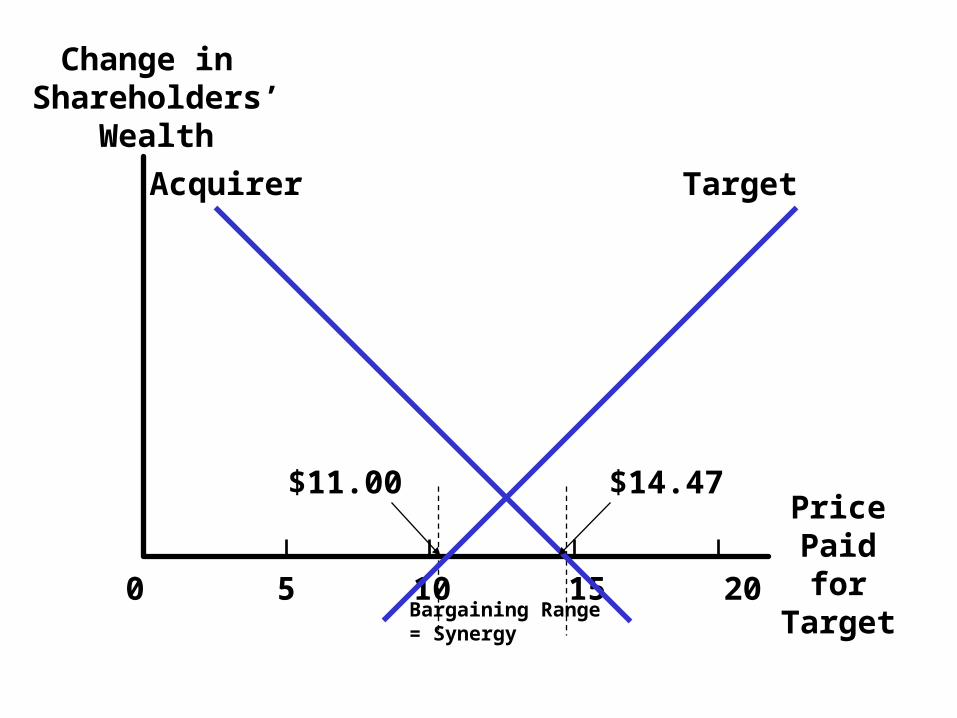
• The offer could range from $11 to $289.4/20 = $14.47 per share.
• At $11, all merger benefits would go to the acquiring firm’s shareholders.
• At $14.47, all value added would go to the target firm’s shareholders.
• The graph on the next slide summarizes the situation.
0 5 10 15 20
Change in Shareholders’
Wealth
Acquirer Target
Bargaining Range = Synergy
Price Paid for Target
$11.00 $14.47

Points About Graph
• Nothing magic about crossover price.
• Actual price would be determined by bargaining. Higher if target is in better bargaining position, lower if acquirer is.
• If target is good fit for many acquirers, other firms will come in, price will be bid up. If not, could be close to $11.
(More...)
• Acquirer might want to make high “preemptive” bid to ward off other bidders, or low bid and then plan to go up. Strategy is important.
• Do target’s managers have 51% of stock and want to remain in control?
• What kind of personal deal will target’s managers get?
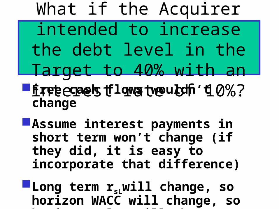
What if the Acquirer intended to increase the debt level in the
Target to 40% with an interest rate of 10%?Free cash flows wouldn’t change
Assume interest payments in short term won’t change (if they did, it is easy to incorporate that difference)
Long term rsLwill change, so horizon WACC will change, so horizon value will change.

New WACC Calculation
New rsL = rsU + (rsU – rd)(D/S)= 11.56% + (11.56% - 10%)(0.4/0.6) = 12.60%
New WACC = wdrd(1-T) + wsrsL
= 0.4(10%)(1-0.4) + 0.6(12.6%)= 9.96%
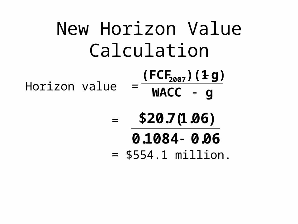
New Horizon Value Calculation
Horizon value =
=
= $554.1 million.
g WACC
g))(1(FCF2007
06.01084.0
)06.1(7.20$

New Vops and Vequity
2004 2005 2006 2007 Free Cash Flow $11.7 $10.5 $16.5 $ 20.7Horizon value 554.1Interest tax shield 2.0 2.6 2.6 2.8Total $13.7 $13.1 $19.1 $577.6
VOps = + + +
= $409.5 million.
$13.7 (1.1156)1
$13.1 (1.1156)2
$19.1 (1.1156)3
$577.6 (1.1156)4
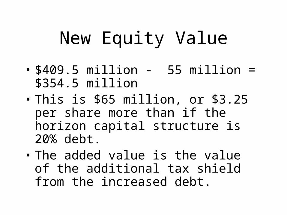
New Equity Value
• $409.5 million - 55 million = $354.5 million
• This is $65 million, or $3.25 per share more than if the horizon capital structure is 20% debt.
• The added value is the value of the additional tax shield from the increased debt.
• According to empirical evidence, acquisitions do create value as a result of economies of scale, other synergies, and/or better management.
• Shareholders of target firms reap most of the benefits, that is, the final price is close to full value.– Target management can always say no.
– Competing bidders often push up prices.
Do mergers really create value?
• Pooling of interests is GONE. Only purchase accounting may be used now.
What method is used to account for for mergers?
(More...)

• Purchase:
– The assets of the acquired firm are “written up” to reflect purchase price if it is greater than the net asset value.
– Goodwill is often created, which appears as an asset on the balance sheet.
– Common equity account is increased to balance assets and claims.

Goodwill Amortization
• Goodwill is NO LONGER amortized over time for shareholder reporting.
• Goodwill is subject to an annual “impairment test.” If its fair market value has declined, then goodwill is reduced. Otherwise it is not.
• Goodwill is still amortized for Federal Tax purposes.

• Identifying targets
• Arranging mergers
• Developing defensive tactics
• Establishing a fair value
• Financing mergers
• Arbitrage operations
What are some merger-related activities of investment bankers?
• In an LBO, a small group of investors, normally including management, buys all of the publicly held stock, and hence takes the firm private.
• Purchase often financed with debt.
• After operating privately for a number of years, investors take the firm public to “cash out.”
What is a leveraged buyout (LB0)?

• Advantages:– Administrative cost savings– Increased managerial incentives– Increased managerial flexibility– Increased shareholder participation
• Disadvantages:– Limited access to equity capital– No way to capture return on investment
What are are the advantages and disadvantages of going private?

• Sale of an entire subsidiary to another firm.
• Spinning off a corporate subsidiary by giving the stock to existing shareholders.
• Carving out a corporate subsidiary by selling a minority interest.
• Outright liquidation of assets.
What are the major types of divestitures?
• Subsidiary worth more to buyer than when operated by current owner.
• To settle antitrust issues.
• Subsidiary’s value increased if it operates independently.
• To change strategic direction.
• To shed money losers.
• To get needed cash when distressed.
What motivates firms to divest assets?
• A holding company is a corporation formed for the sole purpose of owning the stocks of other companies.
• In a typical holding company, the subsidiary companies issue their own debt, but their equity is held by the holding company, which, in turn, sells stock to individual investors.
What are holding companies?
• Advantages:
– Control with fractional ownership.
– Isolation of risks.
• Disadvantages:
– Partial multiple taxation.
– Ease of enforced dissolution.
What are the advantages and disadvantages of holding companies?
What is a real option?
• Real options exist when managers can influence the size and risk of a project’s cash flows by taking different actions during the project’s life in response to changing market conditions.
• Alert managers always look for real options in projects.
• Smarter managers try to create real options.

An option is a contract which gives its holder the right, but not the obligation, to buy (or sell) an asset at some predetermined price within a specified period of time.
What is a financial option?
• It does not obligate its owner to take any action. It merely gives the owner the right to buy or sell an asset.
What is the single most importantcharacteristic of an option?
• Call option: An option to buy a specified number of shares of a security within some future period.
• Put option: An option to sell a specified number of shares of a security within some future period.
• Exercise (or strike) price: The price stated in the option contract at which the security can be bought or sold.
Option Terminology
• Option price: The market price of the option contract.
• Expiration date: The date the option matures.
• Exercise value: The value of a call option if it were exercised today = Current stock price - Strike price.Note: The exercise value is zero if the stock price is less than the strike price.
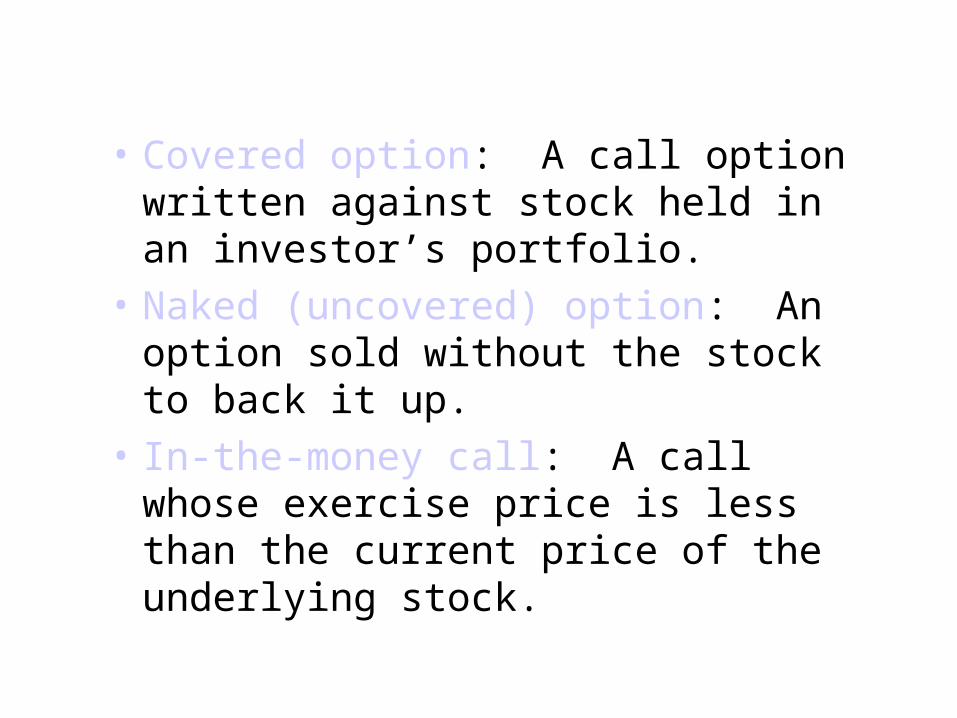
• Covered option: A call option written against stock held in an investor’s portfolio.
• Naked (uncovered) option: An option sold without the stock to back it up.
• In-the-money call: A call whose exercise price is less than the current price of the underlying stock.
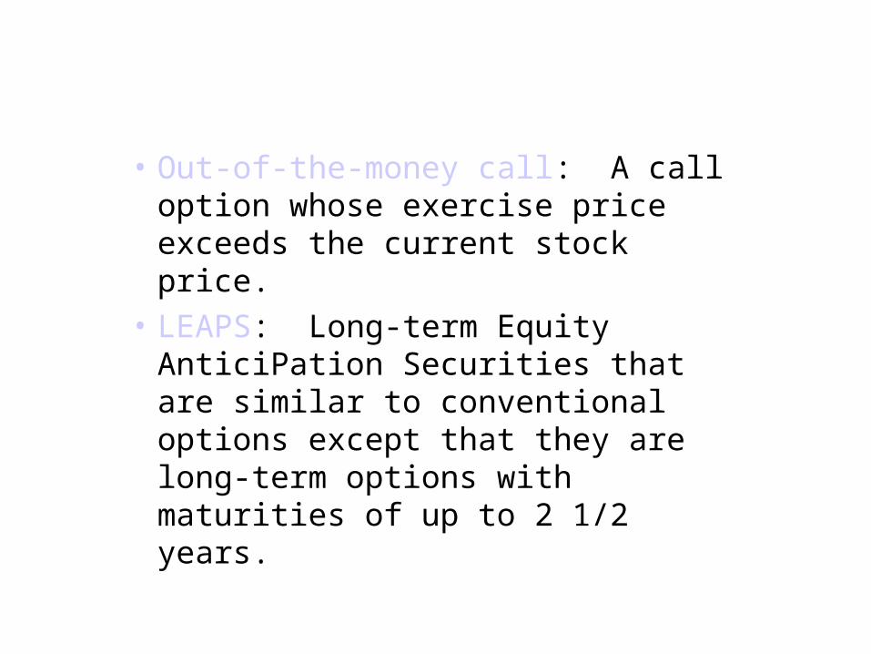
• Out-of-the-money call: A call option whose exercise price exceeds the current stock price.
• LEAPS: Long-term Equity AnticiPation Securities that are similar to conventional options except that they are long-term options with maturities of up to 2 1/2 years.

Exercise price = $25.Stock Price Call Option Price
$25 $ 3.00 30 7.50 35 12.00 40 16.50 45 21.00 50 25.50
Consider the following data:

Create a table which shows (a) stockprice, (b) strike price, (c) exercise
value, (d) option price, and (e) premiumof option price over the exercise value.
Price of Strike Exercise ValueStock (a) Price (b) of Option (a) - (b)$25.00 $25.00 $0.00 30.00 25.00 5.00 35.00 25.00 10.00 40.00 25.00 15.00 45.00 25.00 20.00 50.00 25.00 25.00
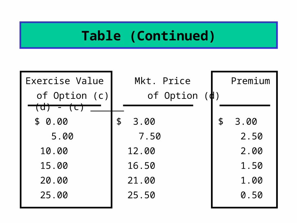
Exercise Value Mkt. Price Premium
of Option (c) of Option (d) (d) - (c)
$ 0.00 $ 3.00 $ 3.00
5.00 7.50 2.50
10.00 12.00 2.00
15.00 16.50 1.50
20.00 21.00 1.00
25.00 25.50 0.50
Table (Continued)
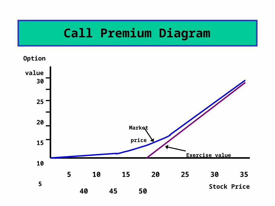
Call Premium Diagram
5 10 15 20 25 30 35 40 45 50
Stock Price
Option value
30
25
20
15
10
5
Market price
Exercise value

What happens to the premium of the option price over the exercisevalue as the stock price rises?
• The premium of the option price over the exercise value declines as the stock price increases.
• This is due to the declining degree of leverage provided by options as the underlying stock price increases, and the greater loss potential of options at higher option prices.

• The stock underlying the call option provides no dividends during the call option’s life.
• There are no transactions costs for the sale/purchase of either the stock or the option.
• RRF is known and constant during the option’s life.
What are the assumptions of theBlack-Scholes Option Pricing Model?
(More...)
• Security buyers may borrow any fraction of the purchase price at the short-term risk-free rate.
• No penalty for short selling and sellers receive immediately full cash proceeds at today’s price.
• Call option can be exercised only on its expiration date.
• Security trading takes place in continuous time, and stock prices move randomly in continuous time.
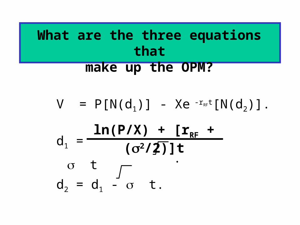
V = P[N(d1)] - Xe -rRFt[N(d2)].
d1 = . t
d2 = d1 - t.
What are the three equations thatmake up the OPM?
ln(P/X) + [rRF + (2/2)]t

What is the value of the following call option according to the OPM?Assume: P = $27; X = $25; rRF = 6%;
t = 0.5 years: 2 = 0.11
V = $27[N(d1)] - $25e-(0.06)(0.5)[N(d2)].
ln($27/$25) + [(0.06 + 0.11/2)](0.5)
(0.3317)(0.7071)
= 0.5736.
d2 = d1 - (0.3317)(0.7071) = d1 - 0.2345
= 0.5736 - 0.2345 = 0.3391.
d1 =

N(d1) = N(0.5736) = 0.5000 + 0.2168 = 0.7168.
N(d2) = N(0.3391) = 0.5000 + 0.1327 = 0.6327.
Note: Values obtained from Excel using NORMSDIST function.
V = $27(0.7168) - $25e-0.03(0.6327) = $19.3536 - $25(0.97045)(0.6327) = $4.0036.
• Current stock price: Call option value increases as the current stock price increases.
• Exercise price: As the exercise price increases, a call option’s value decreases.
What impact do the following para-meters have on a call option’s value?
• Option period: As the expiration date is lengthened, a call option’s value increases (more chance of becoming in the money.)
• Risk-free rate: Call option’s value tends to increase as rRF increases (reduces the PV of the exercise price).
• Stock return variance: Option value increases with variance of the underlying stock (more chance of becoming in the money).
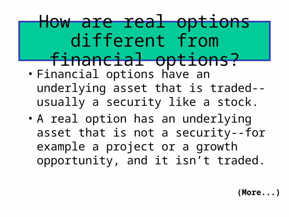
How are real options different from financial options?
• Financial options have an underlying asset that is traded--usually a security like a stock.
• A real option has an underlying asset that is not a security--for example a project or a growth opportunity, and it isn’t traded.
(More...)

How are real options different from financial options?
• The payoffs for financial options are specified in the contract.
• Real options are “found” or created inside of projects. Their payoffs can be varied.
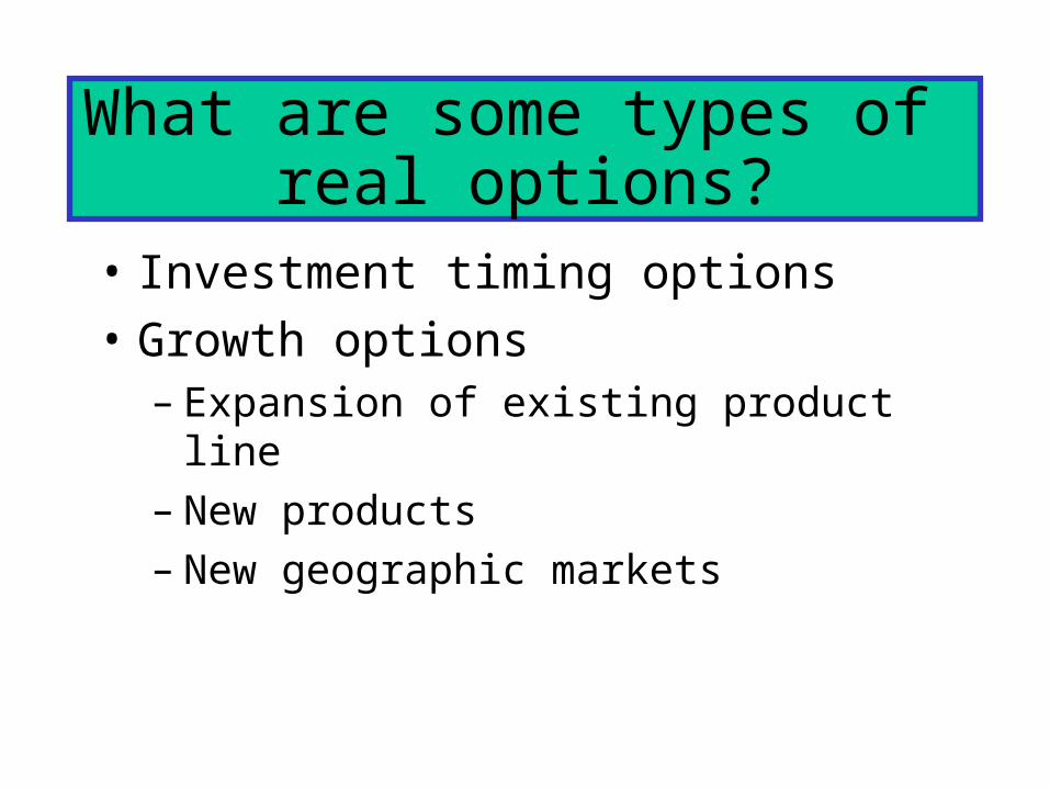
What are some types of real options?
• Investment timing options
• Growth options – Expansion of existing product line– New products– New geographic markets
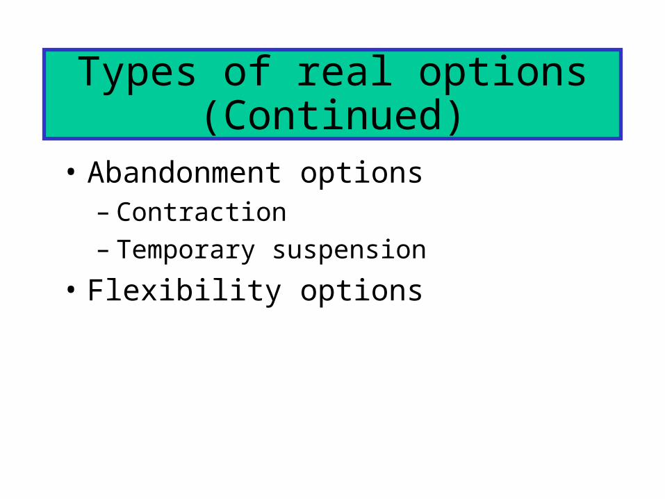
Types of real options (Continued)
• Abandonment options– Contraction– Temporary suspension
• Flexibility options

Five Procedures for ValuingReal Options
1. DCF analysis of expected cash flows, ignoring the option.
2. Qualitative assessment of the real option’s value.
3. Decision tree analysis.
4. Standard model for a corresponding financial option.
5. Financial engineering techniques.
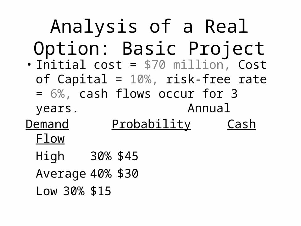
Analysis of a Real Option: Basic Project
• Initial cost = $70 million, Cost of Capital = 10%, risk-free rate = 6%, cash flows occur for 3 years.
AnnualDemand Probability Cash Flow
High 30% $45
Average 40% $30
Low 30% $15

Approach 1: DCF Analysis
• E(CF) =.3($45)+.4($30)+.3($15)
= $30.
• PV of expected CFs = ($30/1.1) + ($30/1.12) + ($30/1/13) = $74.61 million.
• Expected NPV = $74.61 - $70
= $4.61 million
318
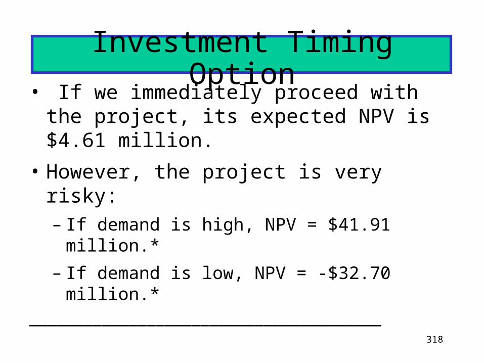
Investment Timing Option• If we immediately proceed with the project,
its expected NPV is $4.61 million.
• However, the project is very risky:– If demand is high, NPV = $41.91 million.*
– If demand is low, NPV = -$32.70 million.*_______________________________________
319
Investment Timing (Continued)
• If we wait one year, we will gain additional information regarding demand.
• If demand is low, we won’t implement project.
• If we wait, the up-front cost and cash flows will stay the same, except they will be shifted ahead by a year.
Procedure 2: Qualitative Assessment
• The value of any real option increases if:– the underlying project is very risky– there is a long time before you must exercise the
option
• This project is risky and has one year before we must decide, so the option to wait is probably valuable.
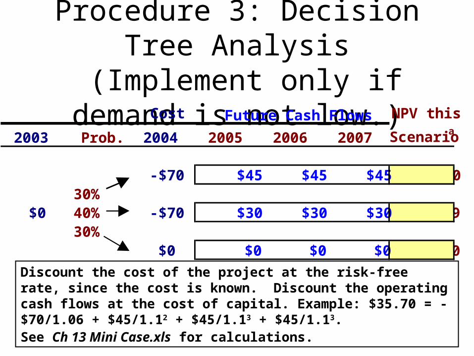
Procedure 3: Decision Tree Analysis
(Implement only if demand is not low.) NPV this
$35.70
$1.79
$0.00
Cost
2003 Prob. 2004 2005 2006 2007 Scenarioa
-$70 $45 $45 $4530%
$0 40% -$70 $30 $30 $3030%
$0 $0 $0 $0
Future Cash Flows
Discount the cost of the project at the risk-free rate, since the cost is known. Discount the operating cash flows at the cost of capital. Example: $35.70 = -$70/1.06 + $45/1.12 + $45/1.13 + $45/1.13. See Ch 13 Mini Case.xls for calculations.
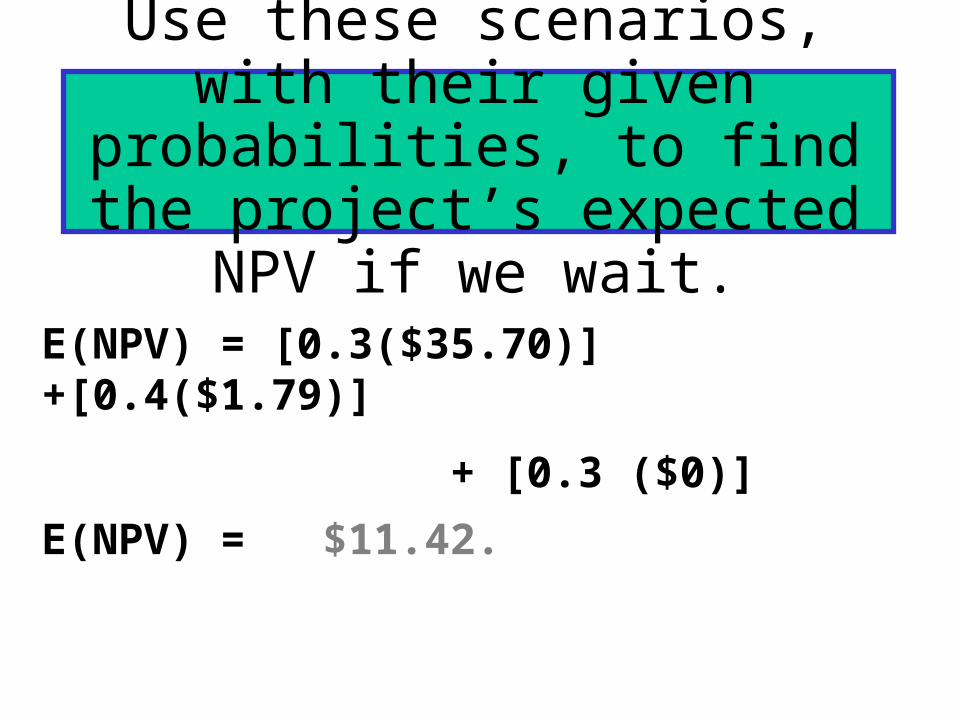
E(NPV) = [0.3($35.70)]+[0.4($1.79)]
+ [0.3 ($0)]
E(NPV) = $11.42.
Use these scenarios, with their given probabilities, to find the project’s expected NPV if we
wait.
Decision Tree with Option to Wait vs. Original DCF Analysis
• Decision tree NPV is higher ($11.42 million vs. $4.61).
• In other words, the option to wait is worth $11.42 million. If we implement project today, we gain $4.61 million but lose the option worth $11.42 million.
• Therefore, we should wait and decide next year whether to implement project, based on demand.

The Option to Wait Changes Risk• The cash flows are less risky under the option
to wait, since we can avoid the low cash flows. Also, the cost to implement may not be risk-free.
• Given the change in risk, perhaps we should use different rates to discount the cash flows.
• But finance theory doesn’t tell us how to estimate the right discount rates, so we normally do sensitivity analysis using a range of different rates.

Procedure 4: Use the existing model
of a financial option.• The option to wait resembles a financial call
option-- we get to “buy” the project for $70 million in one year if value of project in one year is greater than $70 million.
• This is like a call option with an exercise price of $70 million and an expiration date of one year.
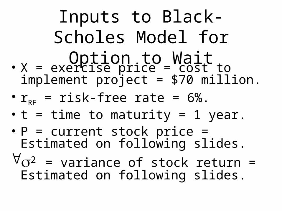
Inputs to Black-Scholes Model for Option to Wait
• X = exercise price = cost to implement project = $70 million.
• rRF = risk-free rate = 6%.• t = time to maturity = 1 year.• P = current stock price = Estimated on following
slides. 2 = variance of stock return = Estimated on
following slides.

Estimate of P• For a financial option:
– P = current price of stock = PV of all of stock’s expected future cash flows.
– Current price is unaffected by the exercise cost of the option.
• For a real option:– P = PV of all of project’s future expected cash
flows.
– P does not include the project’s cost.

Step 1: Find the PV of future CFs at option’s exercise year.
PV at2003 Prob. 2004 2005 2006 2007 2004
$45 $45 $45 $111.9130%40% $30 $30 $30 $74.6130%
$15 $15 $15 $37.30
Future Cash Flows
Example: $111.91 = $45/1.1 + $45/1.12 + $45/1.13.
See Ch 13 Mini Case.xls for calculations.

Step 2: Find the expected PV at the current date, 2003.
PV2003=PV of Exp. PV2004 = [(0.3* $111.91) +(0.4*$74.61) +(0.3*$37.3)]/1.1 = $67.82.
See Ch 13 Mini Case.xls for calculations.
PV2003 PV2004
$111.91High
$67.82 Average $74.61Low
$37.30
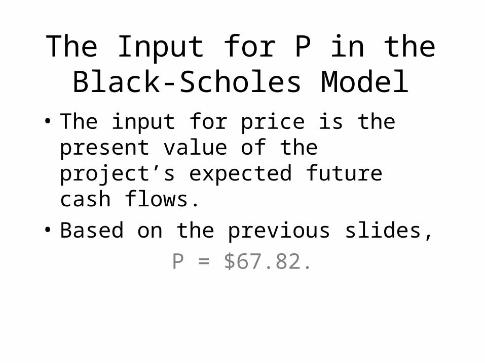
The Input for P in the Black-Scholes Model
• The input for price is the present value of the project’s expected future cash flows.
• Based on the previous slides,
P = $67.82.

Estimating 2 for the Black-Scholes Model
• For a financial option, 2 is the variance of the stock’s rate of return.
• For a real option, 2 is the variance of the project’s rate of return.
Three Ways to Estimate 2
• Judgment.
• The direct approach, using the results from the scenarios.
• The indirect approach, using the expected distribution of the project’s value.

Estimating 2 with Judgment
• The typical stock has 2 of about 12%.
• A project should be riskier than the firm as a whole, since the firm is a portfolio of projects.
• The company in this example has 2 = 10%, so we might expect the project to have 2 between 12% and 19%.
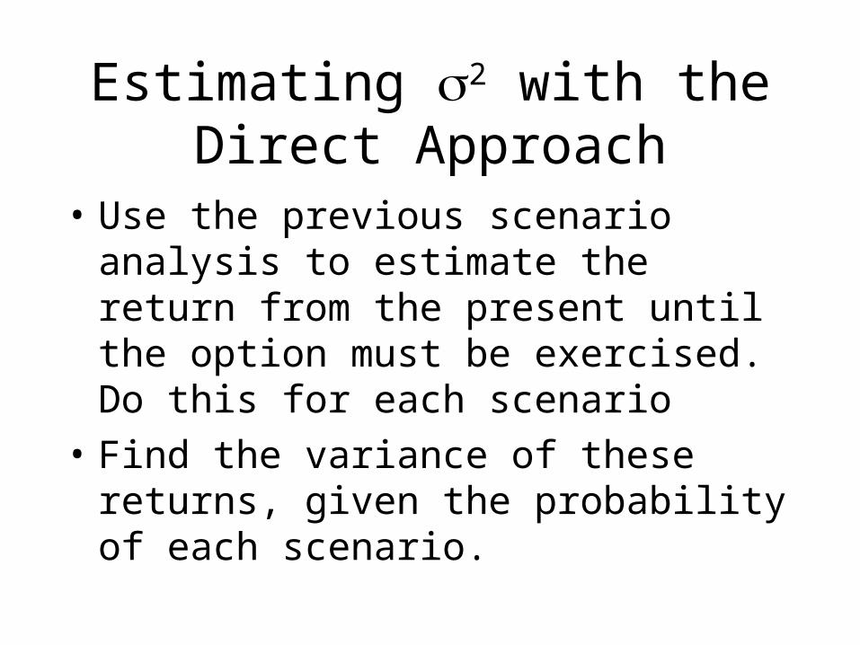
Estimating 2 with the Direct Approach
• Use the previous scenario analysis to estimate the return from the present until the option must be exercised. Do this for each scenario
• Find the variance of these returns, given the probability of each scenario.

Find Returns from the Present until the Option Expires
Example: 65.0% = ($111.91- $67.82) / $67.82.
See Ch 13 Mini Case.xls for calculations.
PV2003 PV2004 Return
$111.91 65.0%High
$67.82 Average $74.61 10.0%Low
$37.30 -45.0%
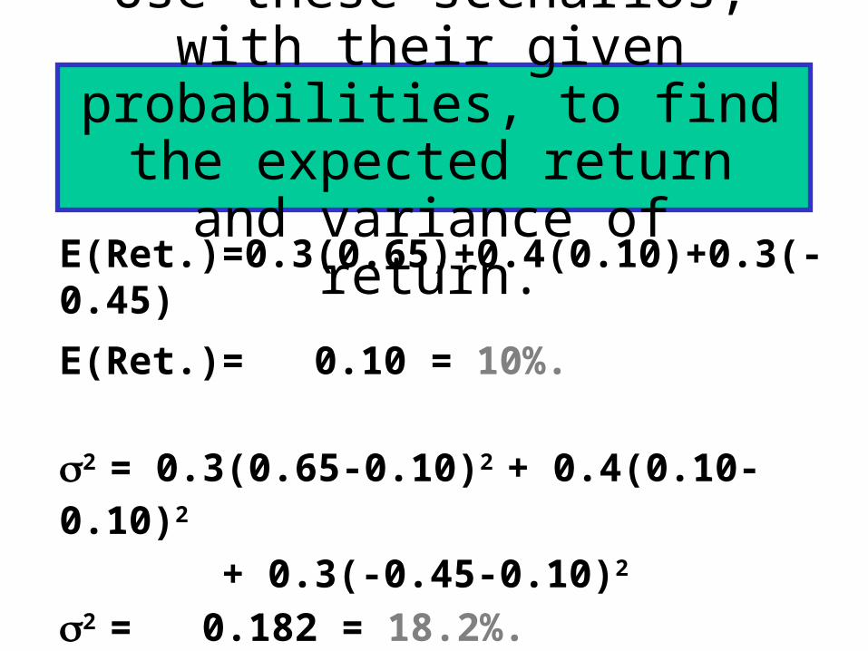
E(Ret.)=0.3(0.65)+0.4(0.10)+0.3(-0.45)
E(Ret.)= 0.10 = 10%.
2 = 0.3(0.65-0.10)2 + 0.4(0.10-0.10)2
+ 0.3(-0.45-0.10)2
2 = 0.182 = 18.2%.
Use these scenarios, with their given probabilities, to find the
expected return and variance of return.

Estimating 2 with the Indirect Approach
• From the scenario analysis, we know the project’s expected value and the variance of the project’s expected value at the time the option expires.
• The questions is: “Given the current value of the project, how risky must its expected return be to generate the observed variance of the project’s value at the time the option expires?”
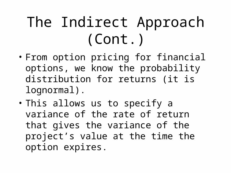
The Indirect Approach (Cont.)
• From option pricing for financial options, we know the probability distribution for returns (it is lognormal).
• This allows us to specify a variance of the rate of return that gives the variance of the project’s value at the time the option expires.

Indirect Estimate of 2 • Here is a formula for the variance of a
stock’s return, if you know the coefficient of variation of the expected stock price at some time, t, in the future:
t
]1CVln[ 22
We can apply this formula to the real option.
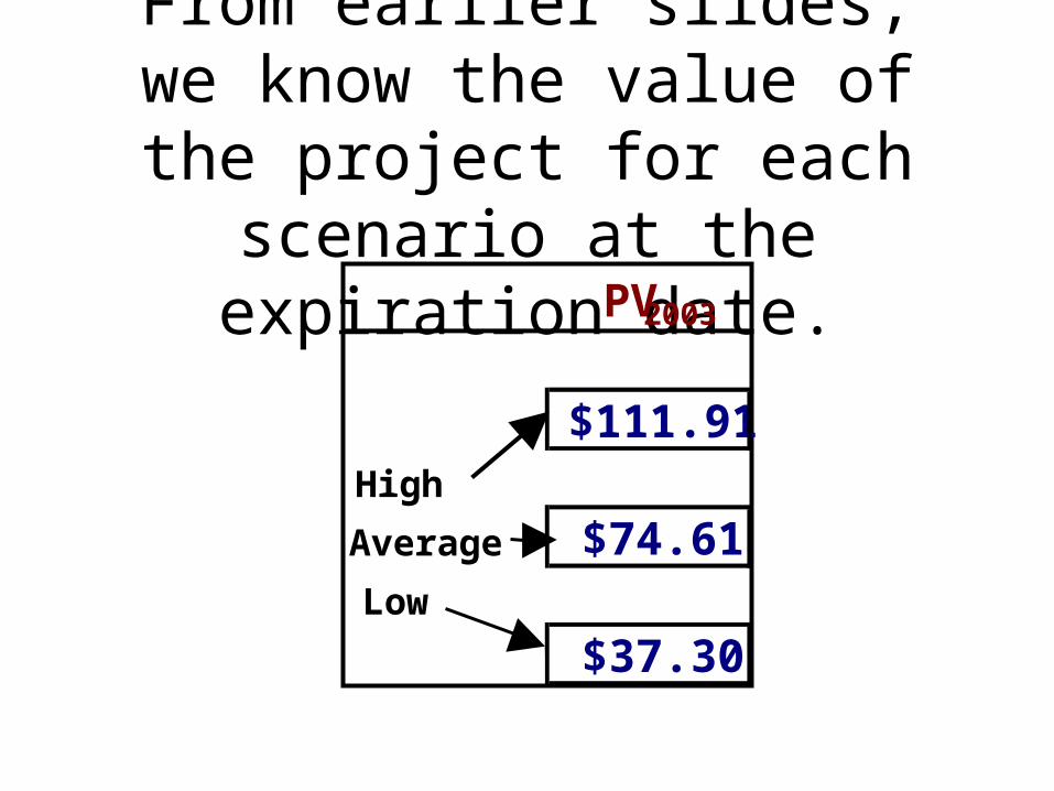
From earlier slides, we know the value of the project for each
scenario at the expiration date.PV2003
$111.91High
Average $74.61Low
$37.30
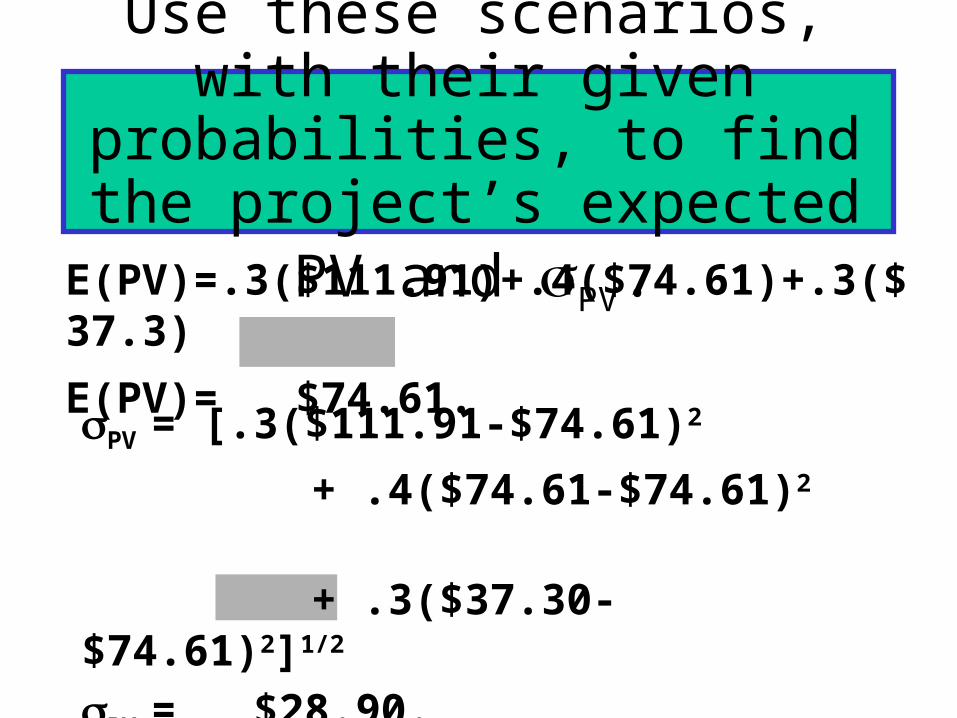
E(PV)=.3($111.91)+.4($74.61)+.3($37.3)
E(PV)= $74.61.
Use these scenarios, with their given probabilities, to find the project’s expected PV and PV.
PV = [.3($111.91-$74.61)2
+ .4($74.61-$74.61)2 + .3($37.30-$74.61)2]1/2
PV = $28.90.
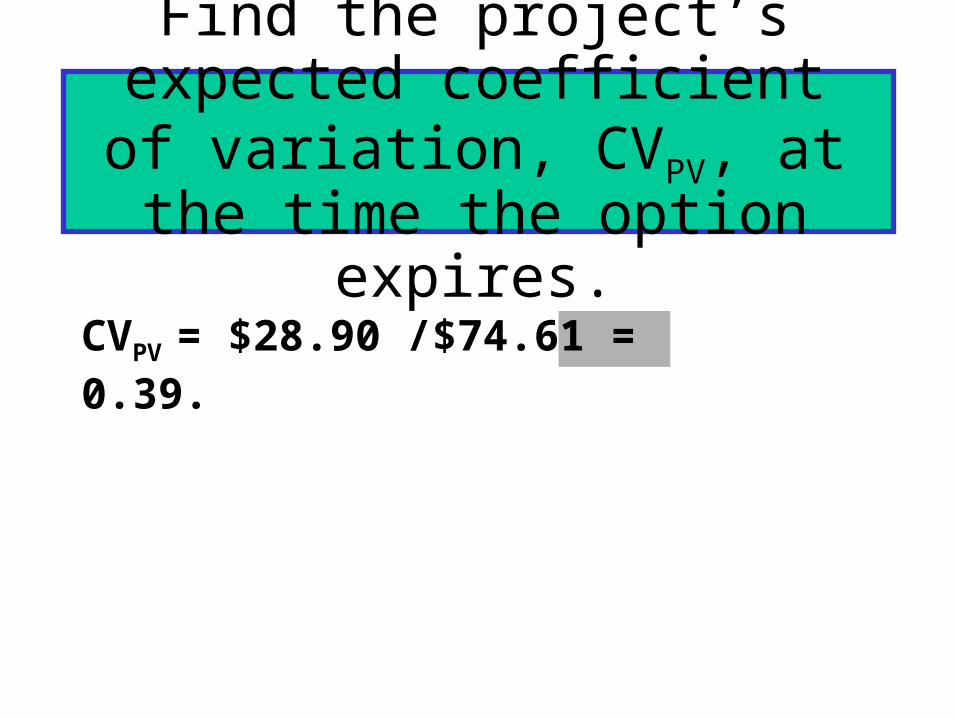
Find the project’s expected coefficient of variation, CVPV, at
the time the option expires.
CVPV = $28.90 /$74.61 = 0.39.
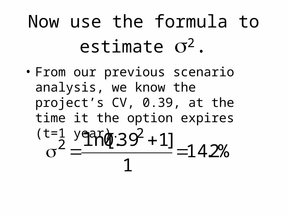
Now use the formula to estimate
2.• From our previous scenario analysis, we
know the project’s CV, 0.39, at the time it the option expires (t=1 year).
%2.141
]139.0ln[ 22

The Estimate of 2
• Subjective estimate:– 12% to 19%.
• Direct estimate:– 18.2%.
• Indirect estimate:– 14.2%
• For this example, we chose 14.2%, but we recommend doing sensitivity analysis over a range of 2.

Use the Black-Scholes Model: P = $67.83; X = $70; rRF = 6%;
t = 1 year: 2 = 0.142
V = $67.83[N(d1)] - $70e-(0.06)(1)[N(d2)].
ln($67.83/$70)+[(0.06 + 0.142/2)](1)
(0.142)0.5 (1).05
= 0.2641.
d2 = d1 - (0.142)0.5 (1).05= d1 - 0.3768
= 0.2641 - 0.3768 =- 0.1127.
d1 =
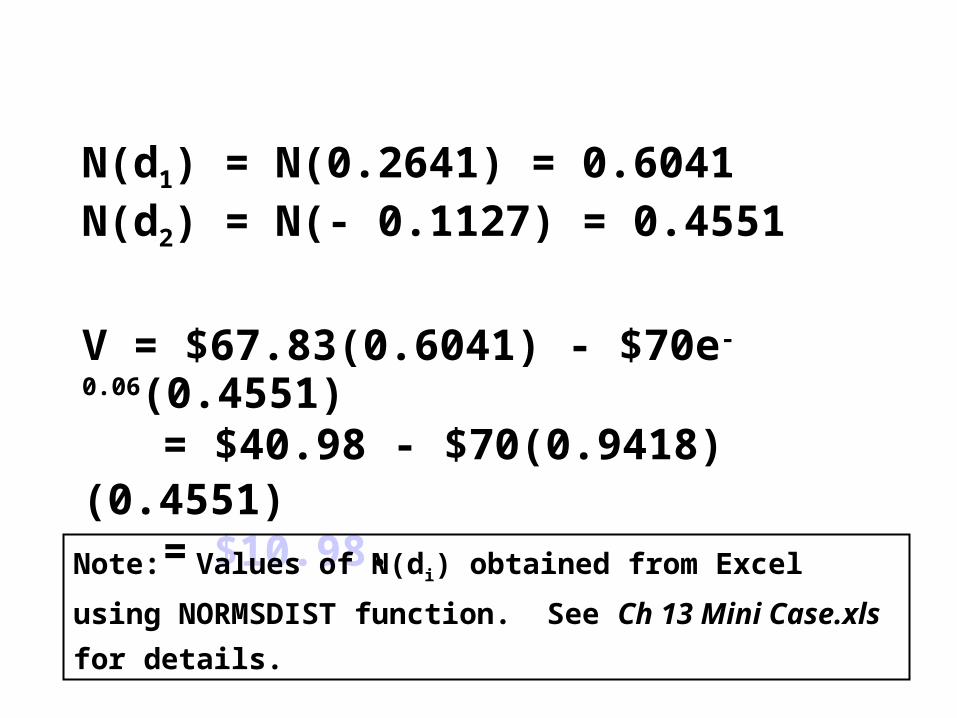
N(d1) = N(0.2641) = 0.6041N(d2) = N(- 0.1127) = 0.4551
V = $67.83(0.6041) - $70e-0.06(0.4551) = $40.98 - $70(0.9418)(0.4551) = $10.98.
Note: Values of N(di) obtained from Excel using
NORMSDIST function. See Ch 13 Mini Case.xls for details.
Step 5: Use financial engineering techniques.
• Although there are many existing models for financial options, sometimes none correspond to the project’s real option.
• In that case, you must use financial engineering techniques, which are covered in later finance courses.
• Alternatively, you could simply use decision tree analysis.
Other Factors to Consider When Deciding When to Invest
• Delaying the project means that cash flows come later rather than sooner.
• It might make sense to proceed today if there are important advantages to being the first competitor to enter a market.
• Waiting may allow you to take advantage of changing conditions.
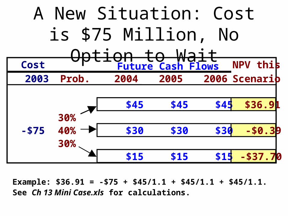
A New Situation: Cost is $75 Million, No Option to Wait
Cost NPV this
2003 Prob. 2004 2005 2006 Scenario
$45 $45 $45 $36.9130%
-$75 40% $30 $30 $30 -$0.3930%
$15 $15 $15 -$37.70
Future Cash Flows
Example: $36.91 = -$75 + $45/1.1 + $45/1.1 + $45/1.1. See Ch 13 Mini Case.xls for calculations.
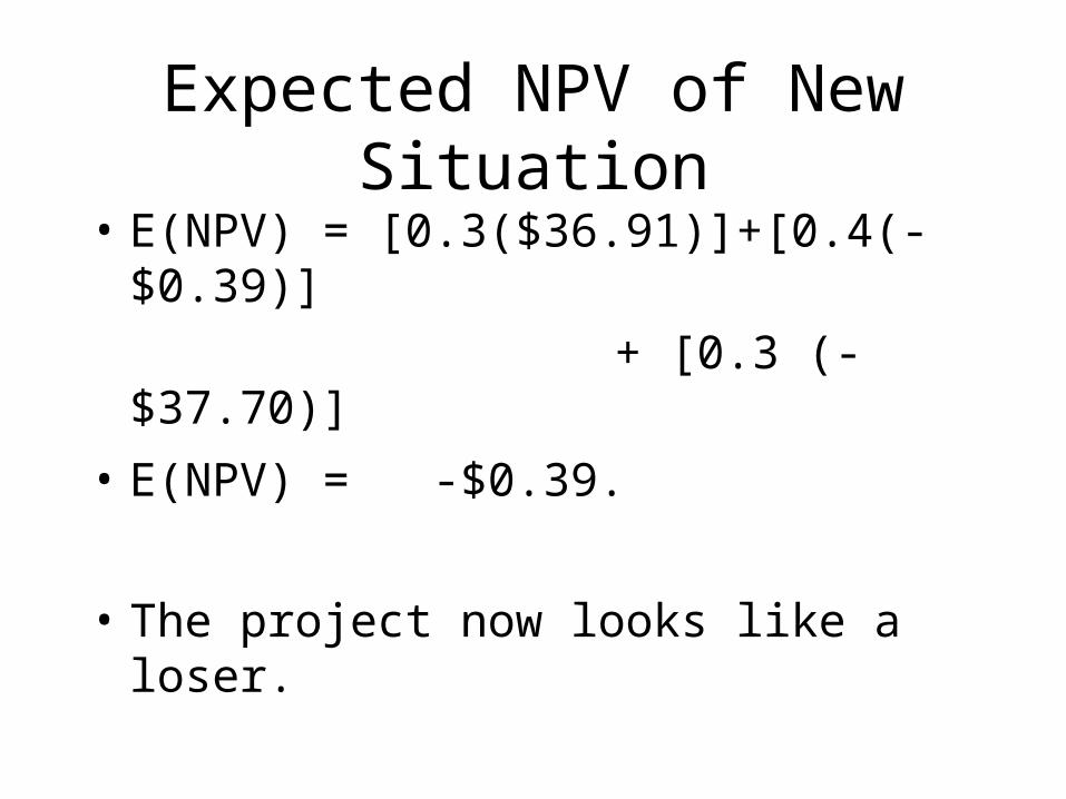
Expected NPV of New Situation
• E(NPV) = [0.3($36.91)]+[0.4(-$0.39)]
+ [0.3 (-$37.70)]
• E(NPV) = -$0.39.
• The project now looks like a loser.

Growth Option: You can replicate the original project after it ends in 3
years.• NPV = NPV Original + NPV Replication
= -$0.39 + -$0.39/(1+0.10)3
= -$0.39 + -$0.30 = -$0.69.
• Still a loser, but you would implement Replication only if demand is high.
Note: the NPV would be even lower if we separately discounted the $75 million cost of Replication at the risk-free rate.
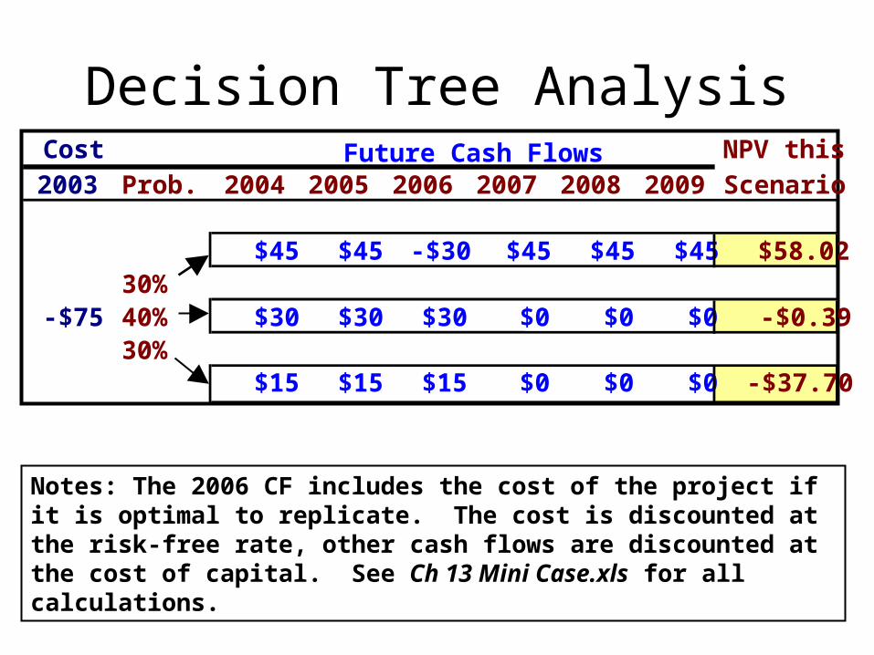
Decision Tree Analysis
Notes: The 2006 CF includes the cost of the project if it is optimal to replicate. The cost is discounted at the risk-free rate, other cash flows are discounted at the cost of capital. See Ch 13 Mini Case.xls for all calculations.
Cost NPV this
2003 Prob. 2004 2005 2006 2007 2008 2009 Scenario
$45 $45 -$30 $45 $45 $45 $58.0230%
-$75 40% $30 $30 $30 $0 $0 $0 -$0.3930%
$15 $15 $15 $0 $0 $0 -$37.70
Future Cash Flows
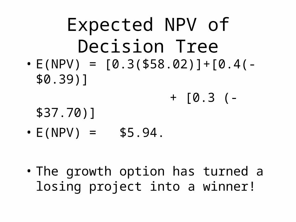
Expected NPV of Decision Tree
• E(NPV) = [0.3($58.02)]+[0.4(-$0.39)]
+ [0.3 (-$37.70)]
• E(NPV) = $5.94.
• The growth option has turned a losing project into a winner!
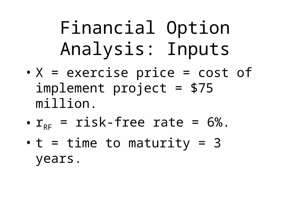
Financial Option Analysis: Inputs
• X = exercise price = cost of implement project = $75 million.
• rRF = risk-free rate = 6%.
• t = time to maturity = 3 years.

Estimating P: First, find the value of future CFs at exercise year.
Example: $111.91 = $45/1.1 + $45/1.12 + $45/1.13.
See Ch 13 Mini Case.xls for calculations.
Cost PV at Prob.
2003 Prob. 2004 2005 2006 2007 2008 2009 2006 x NPV
$45 $45 $45 $111.91 $33.5730%40% $30 $30 $30 $74.61 $29.8430%
$15 $15 $15 $37.30 $11.19
Future Cash Flows
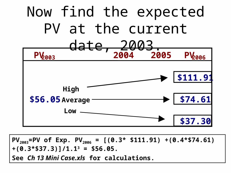
Now find the expected PV at the current date, 2003.
PV2003=PV of Exp. PV2006 = [(0.3* $111.91) +(0.4*$74.61) +(0.3*$37.3)]/1.13 = $56.05.
See Ch 13 Mini Case.xls for calculations.
PV2003 2004 2005 PV2006
$111.91High
$56.05 Average $74.61Low
$37.30

The Input for P in the Black-Scholes Model
• The input for price is the present value of the project’s expected future cash flows.
• Based on the previous slides,
P = $56.05.
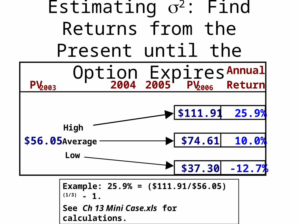
Estimating 2: Find Returns from the Present until the Option
Expires
Example: 25.9% = ($111.91/$56.05)(1/3) - 1.
See Ch 13 Mini Case.xls for calculations.
AnnualPV2003 2004 2005 PV2006 Return
$111.91 25.9%High
$56.05 Average $74.61 10.0%Low
$37.30 -12.7%
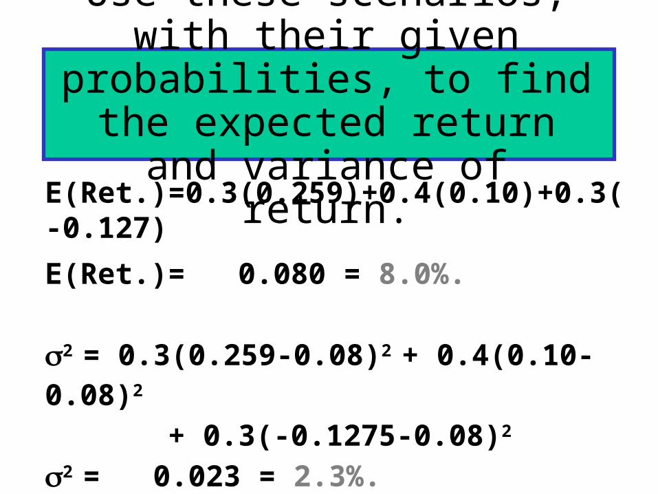
E(Ret.)=0.3(0.259)+0.4(0.10)+0.3(-0.127)
E(Ret.)= 0.080 = 8.0%.
2 = 0.3(0.259-0.08)2 + 0.4(0.10-0.08)2
+ 0.3(-0.1275-0.08)2
2 = 0.023 = 2.3%.
Use these scenarios, with their given probabilities, to find the
expected return and variance of return.
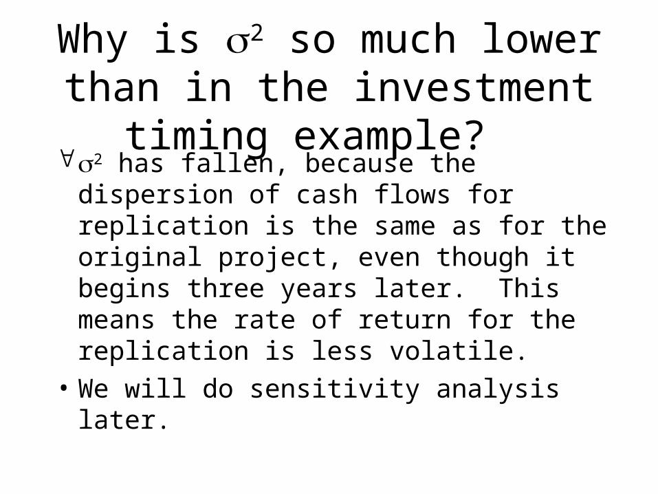
Why is 2 so much lower than in the investment timing example? 2 has fallen, because the dispersion of cash
flows for replication is the same as for the original project, even though it begins three years later. This means the rate of return for the replication is less volatile.
• We will do sensitivity analysis later.

Estimating 2 with the Indirect Method
PV2006
$111.91High
Average $74.61Low
$37.30
• From earlier slides, we know the value of the project for each scenario at the expiration date.

E(PV)=.3($111.91)+.4($74.61)+.3($37.3)
E(PV)= $74.61.
Use these scenarios, with their given probabilities, to find the project’s expected PV and PV.
PV = [.3($111.91-$74.61)2
+ .4($74.61-$74.61)2 + .3($37.30-$74.61)2]1/2
PV = $28.90.
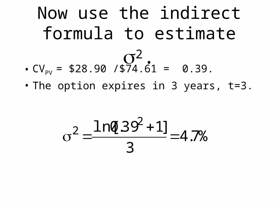
Now use the indirect formula to
estimate 2.• CVPV = $28.90 /$74.61 = 0.39.
• The option expires in 3 years, t=3.
%7.43
]139.0ln[ 22
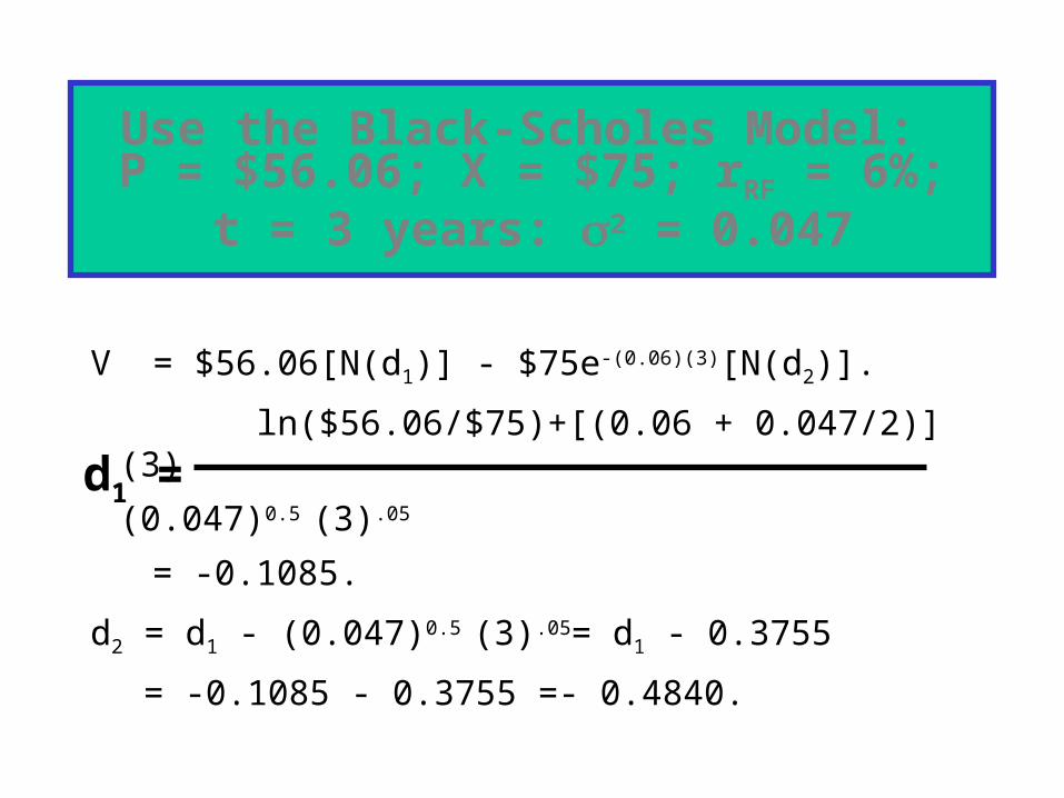
Use the Black-Scholes Model: P = $56.06; X = $75; rRF = 6%;
t = 3 years: 2 = 0.047
V = $56.06[N(d1)] - $75e-(0.06)(3)[N(d2)].
ln($56.06/$75)+[(0.06 + 0.047/2)](3)
(0.047)0.5 (3).05
= -0.1085.
d2 = d1 - (0.047)0.5 (3).05= d1 - 0.3755
= -0.1085 - 0.3755 =- 0.4840.
d1 =
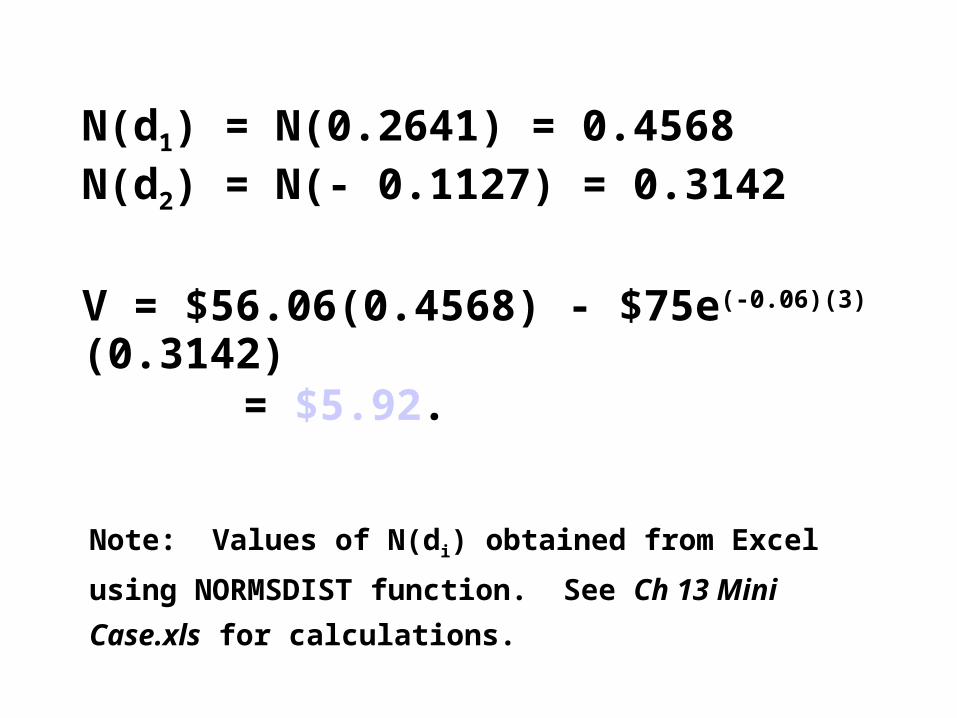
N(d1) = N(0.2641) = 0.4568N(d2) = N(- 0.1127) = 0.3142
V = $56.06(0.4568) - $75e(-0.06)(3)(0.3142) = $5.92.
Note: Values of N(di) obtained from Excel using
NORMSDIST function. See Ch 13 Mini Case.xls for
calculations.

Total Value of Project with Growth Opportunity
Total value = NPV of Original Project + Value of growth option
=-$0.39 + $5.92 = $5.5 million.