Cosmological models,

nonideal fluids

and viscous forces

in general relativity

Daniele Gregoris

Daniele Gregoris is an Erasmus Mundus Joint Doctorate IRAP PhD

student and is supported by the Erasmus Mundus Joint Doctorate

Program by Grant Number 2011-1640 from the EACEA of the

European Commission.

Doctoral Thesis in Theoretical Physics at Stockholm University,

Sweden 2014

Abstract

This thesis addresses the open questions of providing a cosmological modeldescribing an accelerated expanding Universe without violating the energyconditions or a model that contributes to the physical interpretation of thedark energy. The former case is analyzed considering a closed model basedon a regular lattice of black holes using the Einstein equation in vacuum. Inthe latter case I will connect the dark energy to the Shan-Chen equation ofstate. A comparison between these two proposals is then discussed.

As a complementary topic I will discuss the motion of test particles in ageneral relativistic spacetime undergoing friction effects. This is modeledfollowing the formalism of Poynting-Robertson whose link with the Stokes’formula is presented. The cases of geodesic and non-geodesic motion arecompared and contrasted for Schwarzschild, Tolman, Pant-Sah andFriedmann metrics respectively.

c©Daniele Gregoris, Stockholm 2014

Public defense day: 7th November 2014, room FP41 AlbaNova University Center

ISBN 978-91-7447-982-9

Typeset in LATEX

Printed in Sweden by Universitetsservice US AB, Stockholm 2014

Distributor: Department of Physics, Stockholm University

List of Papers

The following papers, referred to in the text by their Roman numerals, areincluded in this thesis.

PAPER I: Radiation pressure vs. friction effects in the description of

the Poynting-Robertson scattering process

D. Bini, D. Gregoris, S. Succi, EPL (Europhysics Letters) 97,40007 (2012)DOI:10.1209/0295-5075/97/40007

PAPER II: Particle motion in a photon gas: friction matters

D. Bini, D. Gregoris, K. Rosquist, S. Succi, General Relativityand Gravitation: Volume 44, Issue 10 (2012),Page 2669-2680doi:10.1007/s10714-012-1425-5

PAPER III: Effects of friction forces on the motion of objects in smoothly

matched interior/exterior spacetimes

D. Bini, D. Gregoris, K. Rosquist and S. Succi, Class. QuantumGrav. 30 (2013) 025009 (17pp)doi:10.1088/0264-9381/30/2/025009

PAPER IV: Friction forces in cosmological models

D. Bini, A. Geralico, D. Gregoris, S. Succi, Eur.Phys.J. C73(2013) 2334doi:10.1140/epjc/s10052-013-2334-9

PAPER V: Dark energy from cosmological fluids obeying a Shan-Chen

nonideal equation of state

D. Bini, A. Geralico, D. Gregoris, S. Succi, Physical Review D88, 063007 (2013)doi:10.1103/PhysRevD.88.063007

PAPER VI: Exact Evolution of Discrete Relativistic Cosmological

Models

T. Clifton, D. Gregoris, K. Rosquist, R. Tavakol, JCAP vol. 11,Article 010, ArXiv 1309.2876doi:10.1088/1475-7516/2013/11/010

PAPER VII: Scalar field inflation and Shan-Chen fluid models

D. Bini, A. Geralico, D. Gregoris, S. Succi, Physical Review D90, 044021 (2014)doi:10.1103/PhysRevD.90.044021

PAPER VIII: Piecewise silence in discrete cosmological models

T. Clifton, D. Gregoris, K. Rosquist, Class. Quantum Grav. 31

(2014) 105012 (17pp), arXiv:1402.3201doi:10.1088/0264-9381/31/10/105012

Proceedings (not included in this thesis):

Kinetic theory in curved space-times: applications to black

holes

D. Bini, D. Gregoris, proceeding for the 12th Italian-KoreanSymposium on relativistic astrophysics,Il nuovo Cimento Vol. 36 C, N. 1 Suppl. 1doi:10.1393/ncc/i2013-11484-7

Friction forces in general relativity

D. Bini, D. Gregoris, K. Rosquist, submitted as proceeding ofthe 13th Marcel Grossmann meeting, 2011

Reprints were made with permission from the publishers.

Contents

Abstract iv

List of Papers v

1 Introduction 9

1.0.1 Notation . . . . . . . . . . . . . . . . . . . . . . . . 10

1.1 The current state of modern cosmology . . . . . . . . . . . 11

1.1.1 Original contribution of this thesis . . . . . . . . . . 13

1.1.2 The author’s contribution to the accompanying

published papers . . . . . . . . . . . . . . . . . . . 15

1.2 The geometric approach: a symmetry group point of view . 16

1.3 The role of the equation of state in cosmology . . . . . . . . 18

1.4 Geometry versus matter content of the Universe . . . . . . 21

1.5 Friction forces in general relativity: formulation of the

problem . . . . . . . . . . . . . . . . . . . . . . . . . . . . . 23

2 Inhomogeneous discrete relativistic cosmology 27

2.1 Motivation of this study . . . . . . . . . . . . . . . . . . . . 27

2.2 The Cauchy formulation of General Relativity . . . . . . . 29

2.2.1 Orthonormal frame approach . . . . . . . . . . . . 31

2.3 Curvature of a discrete mass distribution . . . . . . . . . . 34

2.4 Equations of the dynamics for the discrete models . . . . . 37

2.5 From generic points to particular surfaces, lines and points 39

2.5.1 Reflection symmetry hypersurfaces . . . . . . . . . 40

2.5.2 Lines connecting two masses . . . . . . . . . . . . . 41

2.5.3 Lines connecting two vertices . . . . . . . . . . . . 42

2.5.4 Application of the 1+3 orthonormal frame formalism 42

2.5.5 Commutators and symmetries in the orthonormal

frame approach . . . . . . . . . . . . . . . . . . . . 43

2.6 Summary . . . . . . . . . . . . . . . . . . . . . . . . . . . . 49

3 On the role of the Shan-Chen equation of state in the cosmological

modeling 51

3.1 The Shan-Chen equation of state: a review . . . . . . . . . 523.2 Observational tests . . . . . . . . . . . . . . . . . . . . . . . 57

3.2.1 Late time cosmology . . . . . . . . . . . . . . . . . 573.2.2 Inflationary era . . . . . . . . . . . . . . . . . . . . 603.2.3 A word of warning: the BICEP2 experiment . . . . 63

3.3 Summary . . . . . . . . . . . . . . . . . . . . . . . . . . . . 63

4 Applications of the Poynting-Robertson effect in general relativity 67

4.1 Characterizing a spacetime through the motion of particles 674.2 Motion inside a photon gas in the Schwarzschild metric . . 704.3 Metric curvature versus friction effects . . . . . . . . . . . 734.4 Extending the Poynting-Robertson formalism to the case

of a massive fluid . . . . . . . . . . . . . . . . . . . . . . . 764.5 Peculiar velocities in astrophysics . . . . . . . . . . . . . . 82

Sammanfattning lxxxvii

Acknowledgements lxxxix

References xci

1. Introduction

The modern theory of gravitation formulated as General Relativity is abackbone of the current approach to theoretical physics. In fact it exhibitsmany physical applications for example related to astrophysical phenomenalike the study of black holes, of massive stars, cosmology, cosmogony,gravitational waves and many others. In this thesis I will deal in particularwith cosmological applications of Einstein’s theory discussing two originalcosmological models; at the end I will also speak about the motion ofparticles in general relativistic spacetimes undergoing friction effectscomparing the modified orbits with the geodesic motion. The plan of thepresent thesis is the following:

• In this introductory chapter I will briefly review the most famouscosmological models discussed so far in literature to explain how ouroriginal ones fit inside the current research and the context in whichthey have been formulated. Particular attention will be devoted to therole played by the symmetries of the geometry and the role of theequation of state in the cosmological modeling. Then I will compareand contrast the methods employed in the construction of the two abovementioned models enlightening their merits and suggesting possiblefuture directions of research for refining them. The last part of thechapter introduces the problem of friction forces in general relativitydiscussing its connection with the analogous topic in newtonianmechanics.

• In chapter (2) I will introduce a relativistic inhomogeneous discretecosmological model in vacuum explaining on which assumptions it isbased and summarizing how we improved its understanding. I willfocus my attention on the construction of the initial data for the Cauchyformulation of General Relativity discussing their symmetries whichare inherited by the the complete solution of the Einstein equations. Iwill show how the local rotational symmetry and the reflectionsymmetry constrain the physical variables of the configuration. Anapplication to the propagation of the gravitational waves in theconfiguration can then be derived.

9

• In chapter (3) I will formulate an original cosmological model in whichthe matter content is modeled by a nonideal fluid whose equation of stateexhibits asymptotic freedom. I will mention how this equation of statehas been derived in statistical mechanics by Shan and Chen, its mostimportant features and the observational relations we used to test thetheory with the astronomical observations provided by the current spacemissions.

• Chapter (4) includes instead a digression about the general-relativisticversion of the Poynting-Robertson effect with reference to the Tolman,Schwarzschild, Pant-Sah and Friedmann metrics respectively. Thisforce affects the motion of a massive test particle acting as a dissipativeterm. The results will be discussed with applications to astrophysicsand cosmology. For example the Pant-Sah metric can describe a gascloud which behaves like a gravitational lensing distorting the motionof a body crossing it: our formalism enables us to evaluate thedeflection angle for a particle moving inside it. Moreover we can useour results to estimate the peculiar velocity of an astrophysical objectwhen a cosmological metric is assumed. I would like to mention alsothat friction effects are always present in motion of particles, andusually the computations are only approximations neglecting this kindof effects. Thus the formalism presented in this chapter admits widerapplications also unrelated to cosmology or astrophysics. Our mostimportant original result in this context is the proof that thePoynting-Robertson formula is the correct general relativistic extensionof the famous Stokes’ law.

• At the end of the thesis the reader can find attached the papers Ico-authored. Hence in the next pages I will focus mainly in themethodology adopted, in the initial hypotheses of my work and thefinal conclusions leaving all the details of the full derivation of theoriginal results to the referred articles.

The computations and the plots presented in this thesis and in the attachedpapers have been created with the help of the software for algebraic andsymbolic manipulations MapleTM and MathematicaTM.

1.0.1 Notation

In this paragraph I will introduce the notation used throughout this thesis:

• I will adopt geometric units: G = c = h = 1

10

• Einstein convention of sum over repeated indices is understood

• the metric has signature [-,+,+,+]

• ; and ∇ denote covariant derivative

• round parentheses denote symmetrization: T(ab) = 12(Tab +Tba)

• square parentheses denote antisymmetrization: T[ab] =12(Tab −Tba)

• Volume element for the rest space:

ηαβγ = ηαβγδ uδ = η[αβγ] , (1.1)

where ηαβγδ is the 4-dimensional Levi-Civita symbol.

• Fully orthogonally projected covariant derivative:

∇αT βγ = hβ

δ hργhε

α∇εT δρ (1.2)

• Covariant time derivative along the fundamental worldlines:

T αβ = uγ∇γT α

β (1.3)

• Angle brackets:

v〈α〉 = hαβ vβ , T 〈αβ 〉 =

(

h(αγhβ )

δ −1

3hαβ hγδ

)

T γδ . (1.4)

1.1 The current state of modern cosmology

The search for the correct model describing our Universe is a subject ofconstant debate since the first days of general relativity. The currentconcordance model of cosmology we are familiar with from many textbooksis named Λ-Cold Dark Matter (ΛCDM). It assumes spatial homogeneity andisotropy on large enough scales as working hypotheses and consequently isbased on the Friedmann metric written in comoving Robertson-Walkercoordinates. The matter source is a mixture of perfect fluids like a photon gas,a baryonic matter density, a dark matter and dark energy components. Thesefluids are assumed to be non-interacting and hence they are separatelyconserved. The experimental observations, like the ones coming from thestudy of the type Ia supernovae, the analysis of the cosmic microwavebackground and of the baryonic acoustic oscillations, are then fitted to derivethe amount of the different matter contents of the Universe. The orthogonal

11

plots which can be created by superimposing the above mentionedobservations, after fixing a Friedmann metric as a background, are currentlyinterpreted in terms of an almost spatially flat Universe dominated by a darkenergy fluid, compatible with the cosmological constant term entering theEinstein equations, which in particular gives raise to an accelerated expansionof the Universe [1; 2].

The symmetries of the theory of general relativity does not forbid thepresence of this latter term, but its physical nature and consequently the oneof the dark energy has not been established up to now. The current literaturecontains many theoretical proposals which address the question of thephysical interpretation of the dark energy. For example the dark energy hasbeen modeled as a quintessence fluid [3; 4], or the existence of modified andexotic equations of state, the most popular of them being nowadays theChaplygin gas [5–7], have been considered. This latter case has also beencompared to the k-essence model whose lagrangian can be formulated interms only of its kinetic part like in the Born-Infeld theory [8–10].Braneworld models, scalartensor theories of gravity and modified/massivegravity models play some role in the current research [11; 12]. Other authorsdescribe the large scale accelerated expansion of the Universe invoking thebulk viscosity of scalar theories [13], while others analyzed the effects ofsmall local inhomogeneities and of the formation of structures on the globaldynamics of the Universe. In this latter case both perturbative [14–16] andnon perturbative approaches [17–19] have been adopted to evaluate theso-called backreaction. This term follows from the non-commutativity of theaveraging operation over small scale structures and of the Einstein fieldequations. The two complementary methods for the analysis of spatialinhomogeneities are referred to as top-down and bottom-up approaches[20–22]. In the former we begin with a completely homogeneous backgroundto which we then add some perturbations which should mimic the observedastronomical structures. In the latter the point of view is the opposite: webuild up a cosmological model starting from the truly observed structures inthe physical Universe, i.e. galaxies and clusters of galaxies, and deriving thenthe consequent large scale dynamics which in this case can be considered asan emergent property of the system resulting from the interaction between thedifferent constituents. The most important aim of this specific proposal is tosolve the structure formation problem and the accelerated expansion of theUniverse together without violating the energy conditions. For the state of theart in the analysis of inhomogeneities in the cosmological modeling see[23–29] and references therein. I would like to warn the reader that I justnamed few of the most important lines of research to give an idea of howmuch the work about the dark energy problem is important, and not to review

12

all the possible analysis published so far. The reader can find the references tothese approaches in the bibliographies of the attached papers.

To summarize, the current research in theoretical cosmology falls mainlyinto two different lines: one can act on the l.h.s or on the r.h.s of the Einsteinequations

Gµν +Λgµν = 8πTµν , (1.5)

where

Gµν = Rµν −1

2Rgµν (1.6)

is the Einstein tensor, Rµν and R being the Ricci tensor and scalar respectivelyfunction of the metric gµν and its derivatives, Λ is the above mentionedcosmological constant and Tµν the stress-energy tensor.

In the former case we act on the geometry of the Universe usuallyrelaxing the initial assumptions of perfect homogeneity and isotropy (i.e.reducing the symmetry group of the geometry), while in the latter we usuallymaintain the assumptions that we can base geometrically our model on theFriedmann metric and we modify the matter content involved in thestress-energy tensor for example considering not only simple polytropicequations of state for the fluids entering the stress-energy tensor. Again in theformer case the aim is to account for the observational data without the needof any dark side of the Universe or any cosmological constant or any exoticfluids looking for new and original exact or approximate solutions of theEinstein field equations. In the latter, overturning the point of view, wepostulate the existence of some exotic fluid permeating the Universe whichbehaves like dark energy to explain its physical nature: the starting point is alagrangian formulation motivated from microscopic arguments (usually fromthe theory of elementary particles), which is connected to an effectiveequation of state through the canonical equations whose free parameters arethen constrained by the experimental observations.

1.1.1 Original contribution of this thesis

During my Ph.D., performed inside the project “Erasmus Mundus joint IRAPPh.D. program”for relativistic astrophysics, I have analyzed both theseapproaches.

In one case, under the supervision of prof. Kjell Rosquist and incollaboration with Dr. Timothy Clifton and Prof. Reza Tavakol, we haveconsidered a spatially closed Universe in vacuum made by a regular lattice ofan increasing number of non-rotating and uncharged Schwarzschild blackholes. They are supposed to be a rough schematization of the observed

13

astronomical structures like galaxies and clusters of galaxies: their positionshave been fixed by tiling a 3-sphere with regular polychora (four-dimensionalanalogue of the platonic solids). This model is part of the research in thebottom-up approach to inhomogeneous cosmology: this is a genuinelyinhomogeneous model on small scale and instead approaches a homogeneousone on large scale after coarse-graining. Moreover this is a fully generalrelativistic exact non-perturbative model which does not possess any globalcontinuous symmetry. Its dynamics can thus be completely solvedanalytically during all the evolution of the system only along special linesadmitting local rotational symmetry, examples of them being the edges of thecells and the lines connecting two masses. The face of the cell, whose centeris occupied by the black hole, admits instead invariance under reflection thatcan be exploited to derive some conclusions about the propagation ofgravitational waves in these models. The kinematical quantities like theexpansion rate, the shear tensor, the spatial gravito-electric andgravito-magnetic Weyl tensors have been discussed on these lines andsurfaces. In particular we can follow the time evolution of the length of somespecial lines and we can introduce a Hubble function and a decelerationparameter based on this length, formally in the same way as in the Friedmannmodel where they are instead defined in terms of the scale factor. It turns outthat different regions of the space-time admit completely different behaviors.The results have also been compared with the ones of the simpler Friedmannmodel. We can also show that the discrete symmetries of the face inducethese models to be piecewise silent, and consequently they are more realisticthan previously considered silent models.

On the other hand, under the supervision of Drs. Donato Bini, SauroSucci and Andrea Geralico, I have considered a Friedmann model withoutcosmological constant whose matter content is given by the Shan-Chennon-ideal equation of state with asymptotic freedom with the purpose ofgiving a physical interpretation of nature of dark energy. This is a modifiedequation of state introduced in the framework of kinetic lattice theorydescribing a fluid which behaves like an ideal gas (pressure and densitychange in linear proportion to each other) at both low and high densityregimes (for this reason we speak of asymptotic freedom), with a liquid-gascoexistence loop in between. This equation of state has also been compared tothe bag model of hadronic matter and thus a cosmological application is wellmotivated because the Shan-Chen equation of state is not just a numericaltrick. We showed that when we plug this equation of state in the Einsteinequation we can evolve from an initially radiation dominated universe, asrequired by the hot big bang model, to a dark energy dominated one. Thismeans that we have a phase transition in which the pressure switches its sign

14

at a certain instant in the past and stays negative for a long time intervalincluding the present day. After adding a pressure-less matter content to ourpicture of the Universe, we proved that our model can fit the supernova datawhere the distance modulus is plotted with respect to the redshift for anappropriate choice of the free parameters entering the equation of statewithout any need of vacuum energy. We also showed that for this specificchoice of the parameters inside the equation of state, our model is stableunder small initial perturbations and so is self-consistent. In this way we canprovide a microscopic interpretation of the dark energy when we take intoaccount the form of the potential modeling the interaction on which thisequation of state is based. We also applied the model to the description of theinflationary era of the Universe evaluating the experimental quantities like theratio of tensor to scalar perturbations, the scalar spectral index and itsrunning. A graceful exit mechanism from the inflationary era is also providedby this model.

1.1.2 The author’s contribution to the accompanying published

papers

I will explain in this section my personal contribution to the attached papersthat I co-authored.

In papers I-IV my work consisted mainly in deriving the equations ofmotion and in solving them generating the plots for the particle orbit. Beforethe beginning of this analysis I was trained on the use of the softwareMapleTM in similar but simplified situations than the ones consider in thisseries of papers. I also proposed the extension of the Poynting-Robertsonformalism to the case of motion inside a massive fluid subsequentlyre-interpreted in terms of the analogy with the Stokes’ law and theintroduction of direct and indirect interaction between test particle and fluid.

I re-derived independently all the results discussed in paper V and VII,where in the latter I played a major role in clarifying the role of themeasurable quantities in the physical situation under exam and theirconnection with respect to our specific cosmological model and in proposingan application of the Shan-Chen equation of state to the inflationary epoch.

In paper VI I focused my attention mainly in the 5 and 8 massconfigurations, in their lattice construction, in the initial data construction andin the derivation of the dynamical equations in these specific cases; in paperVIII I calculated the explicit simplifications of the gravito-electric,gravito-magnetic and shear tensors on the reflection symmetry surfaces wewere dealing with.

I took active part in all the discussions underlying all the papers I am

15

submitting for my final dissertation not only providing handwrittencomputations and the MapleTM and MathematicaTM codes for the quantitativederivation of the results presented but also in suggesting their connection tothe broader scientific context inside which I have been working and in writingpreliminary versions of the manuscripts (note the alphabetic ordering of thenames of the authors in the attached papers).

1.2 The geometric approach: a symmetry group point

of view

In the next chapter I will demonstrate that the Einstein equations (1.5)constitute a system of non-linear partial differential equations. Thus theirsolution is not known in general. To find manageable solutions usually somesymmetries are imposed as assumptions at the very beginning: this has beendone also in cosmology. Then the derived solution must be compared with theastrophysical observations to see if the mathematical result represents also aphysical meaningful one. In this section I will review the role played by thespace-time symmetry group in the development of some remarkablecosmological models.

As already stated the Friedmann-Lemaître-Robertson-Walker (FLRW)models, derived from the hypotheses of spatial homogeneity and isotropy toaccount for the cosmological principle, agree very well with the astronomicaldata sets in the description of our Universe only by introducing a dark andundetected side of the Universe. The Friedmann metrics are solutions of theEinstein equations (1.5) where the matter content is described by thestress-energy tensor

Tαβ = (p+ρ)uαuβ + pgαβ (1.7)

for a perfect fluid assumed to be at rest with respect to the coordinates with p

denoting the pressure, ρ the energy density and uα = (1,0,0,0) thefour-velocity of the geodesic congruence. To take into account also theobservational constraint of an expanding Universe (formulated by the Hubblelaw) the metric has been chosen in the form

ds2 = −dt2 +a2[

dr2 +Σ2k(dθ 2 + sin2 θdφ 2)

]

, (1.8)

where a = a(t) is the scale factor, while the function Σk(r) = [sinr,r,sinhr]assumes different expressions reflecting the curvature of a spherical, flat andhyperbolic universe respectively, and k = −Σ′′/Σ, where a prime denotesderivative with respect to r. An equation of state p = p(ρ) relating thepressure and the energy density of the fluid must be chosen to have a closedsystem of equations.

16

The simplest and most symmetric model belonging to this family is theEinstein static model which is based on the line element (1.8) with k = +1and a = const. This model is homogeneous both in space and time andisotropic in space. To obtain a static solution it is necessary to impose arelation of the type Λ = 1

2(ρ + p) between the cosmological constant, theenergy density and the pressure of the fluid permeating the Universe [30].However the discovery of the expansion of the Universe mathematicallyexpressed by the Hubble law clearly showed that this mathematical solutionwas not the one chosen by nature [31].

Thus to improve our description of the physical Universe, the staticassumption has been removed moving to the class of the Friedmannexpanding models [32]. In this context the assumptions of spatialhomogeneity and isotropy are maintained, and thus the energy density, thepressure and the scale factor are function of the time only. The Einsteinequations (1.5) in this case are reduced to the Friedmann equation expressingthe evolution in time of the scale factor

a2 = −k +8

3πρa2 , (1.9)

where a dot corresponds to derivative with respect to the time, and the energyconservation equation

ρ = −3a

a(ρ + p) , (1.10)

where a fluid with p = −ρ can mimic the cosmological constant Λ. Withfurther assumptions on the spatial curvature and on the type of fluid, a setof geometrical cosmological solutions can be derived, the most famous onesbeing the de Sitter [33], anti de Sitter, Milne [34] and Eintein-de Sitter ones[35]. As I mentioned above the Friedmann class of solutions are the basis ofthe concordance model of cosmology.

However in this picture the existence of astronomical structures iscompletely neglected. Two approaches can now be followed: add someperturbations on a fixed Friedmann background and follow their evolutions orlook for other exact solutions. We will consider in this thesis the latter case.For example if one wants to eliminate the hypothesis of isotropy it is possibleto substitute the scale factor a(t) with a family of two or three scale factorsa1(t), a2(t), a3(t), which are again only function of the time because we arestill considering a homogeneous Universe. In this case we refer to the scalefactor of the Universe as the quantity a = (a1 a2 a3)

13 [36]. On the other hand

if we want to consider an inhomogeneous Universe the scale factor, theenergy density and the pressure must be function also of the spatialcoordinates and not only of the time. For example the first step is to consider

17

an inhomogeneous Universe admitting spherical symmetry, mathematicallymeaning that a(t) → a(t,r) (then we can of course consider different scalefactors along the different spatial directions to obtain an even more generalsolution) [37]. As a next step the scale factor must be allowed to be functionalso of the angular coordinates. In these cases analytical solutions are notavailable, but the dynamics of the Universe can be treated at leastqualitatively exploiting a dynamical system formalism. In the next chapter Iwill apply it for particular points of the configurations considered in ouroriginal model. For a complete classification of the most famouscosmological models in terms of their symmetries see [38].

The real Universe is of course less symmetric than the solutions availablein literature. Moreover we can hypothesize that the postulated existence ofan exotic and undetected fluid like the dark energy in the Λ-CDM model canbe a consequence of a naive choice of the metric. It is then worthy to relaxeven more the initial assumptions about the symmetries of the geometry ofthe Universe, as I will do in the second chapter of this thesis where I willdeal with an inhomogeneous discrete model. I would like to stress now thatthe above mentioned symmetries are continuous and are thus connected to thepresence of a Killing vector field of the metric. As a next step in relaxing theseassumptions I will consider a model admitting only discrete symmetries. Torealize this project I will consider a regular lattice of black holes playing therole of the astronomical structures. Appropriately arranging the Schwarzschildmass sources, there would be points and lines which admit local rotationalsymmetry and surfaces which exhibit instead symmetry under reflection. Wewill treat the symmetries as follow: after constructing the initial data we willsee what kind of symmetries they exhibit; then it is possible to prove that theirsymmetries are inherited by the complete solution of the Einstein equations.When we will consider a discrete symmetry, we must define it not in terms ofKilling vector fields, but in terms of a diffeomorphism between the spacetimemanifold and itself which preserves the first and second fundamental forms.See [39; 40] for the proofs of such theorems about the preservations of theinitial symmetries along all the time evolution of the system.

1.3 The role of the equation of state in cosmology

In this paragraph I will introduce a complementary approach to cosmologythan the one discussed in the previous section. In fact I will maintain that theassumptions of spatial homogeneity and isotropy of the Friedmann class ofcosmological models are well motivated at least on large scales. Theinterpretation of the space mission data in this framework implies the presentepoch of the Universe to be dark energy-matter dominated; the goal is now to

18

picture physically the characteristics of this exotic fluid. In this section I willoutline the procedure usually adopted to reach this target.

First of all it is well known that in nature three fundamental forces exist:the electroweak, strong and gravitational interactions. The first two can besuccessfully described by the theory of relativistic quantum field and are thedominant ones on microscopic scales. On the other hand we assume that inthe late time cosmology the only force playing a role is the gravitational one.However it has not been possible so far to provide a physical interpretationof the dark energy in the framework of these fundamental forces: up to nowtogether with the mass density it is only a parameter of the fit of the standardmodel of cosmology after assuming a Friedmann metric as background, asalready explained.

Once admitted that the dark energy can really be a physical component ofour Universe, even if not yet detected, and not only an unwanted consequenceof the chosen metric, the challenge is to set it in terms of a well posed fieldtheory. The method usually adopted in this context is the following:

• We start from a lagrangian formulation in terms of a complex scalarfield: the action of the cosmological model is usually provided by thetheory of elementary particles; I stress that the action itself is not ameasurable quantity and consequently can not be compared directly toexperimental data and consequently observational relations must bederived.

• From the lagrangian, the Friedmann metric and the definition of thestress-energy tensor in terms of the pressure and energy density of thefluid, we can derive the canonical equations which connect the scalarfield to the pressure and energy density of the fluid that it describes.

• We eliminate the scalar field from the canonical equations to obtain a“phenomenological”equation of state for the fluid stating the pressure interms of the energy density; usually this equation of state contains oneor two free parameters not fixed by the initial assumptions.

• We plug this equation of state inside the Einstein equations, which arenow constituted by the Friedmann and energy conservation equations,and solve them obtaining the evolution of the energy density and of thescale factor as functions of the time.

• We use these solutions to fit the observed data, for example plottingthe the distance modulus and/or the Hubble function with respect to theredshift, or reconstructing the cosmic microwave background and thebaryonic acoustic spectra. If we can fit all the observations with the

19

same interval for the free parameters of the equation of state, the theorycan be considered compatible with the observations.

• As a final check it is necessary to show that the model is self-consistent:it must be stable under small perturbations.

In real life, it can happen that we start fitting the observed data with aparametric equation of state ad hoc and then the lagrangian is inferredintegrating the canonical equations. A remarkable example in this direction isthe modified Chaplygin gas formulated by a two-parameter equation of stateof the form

p = − A

ρα. (1.11)

In fact in a recent paper [5] its relation to the Nambu-Goto string action plussoft-core corrections has been analytically derived, while in a series of otherpapers the free parameters have been constrained using the astronomical dataset [6; 7].

Following the same procedure, we have considered the modified equationof state with asymptotic freedom of Shan-Chen [41]; it is possible to showthat:

• This equation of state can be compared to the quark model for hadrons.

• Plugging this equation of state inside the Einstein equations (1.5) it ispossible to evolve naturally from a radiation dominated Universe to adark energy dominated one without the need of any vacuum energy: thepressure switches sign at a certain instant in the past remaining negativefor a long time interval which includes the present era.

• It replaces the repulsive action of the cosmological constant with apurely attractive interaction with asymptotic freedom.

• With an appropriate choice of the free parameters we can fit the typeIa supernova data, the scalar spectral index, its running and the ratio oftensor to scalar perturbations.

• This model is stable under small perturbations for the same choice ofparameters.

• This equation of state admits an interpretation in terms of a chameleonscalar field.

• It provides a natural exit mechanism from the inflationary era of theUniverse, which instead is not present in the previous modeling of thedark energy in terms of the cosmological constant.

20

I refer to chapter 3 of this thesis and to papers V and VII and referencestherein for more details about the derivation of the above mentioned equationof state by Shan and Chen in the framework of the lattice kinetic methodsemployed in statistical mechanics, and the observational tests we applied. Iwould like to stress here instead the relationship between a physicalinteraction and an equation of state [42]. In fact if a microscopic potentialU = U(r) describes the interaction between the particles constituting thefluid, the statistical mechanics methods allow us to derive a virial expansionof the equation of state where the pressure is expressed through a power seriesof the density N/V :

p

T=

N

V+B2(T )

(

N

V

)2

+B3(T )

(

N

V

)3

+ ... , (1.12)

as a function of the potential, where T denotes the temperature. The secondcoefficient of this expansion is for example given by

B2(T ) = −1

2

∫

dr(e−βU −1) , (1.13)

where β is the inverse temperature. This well-known example shows that alsoin cosmology we can reconstruct the properties of the fluid permeating theUniverse by fitting the data sets, and then connect this fluid to a fundamentalinteraction using the methods of statistical mechanics.

1.4 Geometry versus matter content of the Universe

In the second and third chapter of this thesis I will introduce two different andoriginal models for relativistic cosmology. As explained there and in theattached papers they belong to two completely different and opposite schoolsof thinking appearing nowadays in the scientific debate. The initialassumptions are consequently not the same and according to me they deserveto be discussed in some details once again even more than the conclusionsthey imply. Any theory or model with the ambitions of describing the natureand the physical world we are living in must clearly separate and distinguishbetween what we assume, what we derive, what we observe and what we

interpret; cosmologists must always remember and apply these steps.In the specific case of this thesis I have discussed two models both

exhibiting an accelerated expansion Universe; in the concordance model ofcosmology such dynamical behavior is explained in terms of the presence of adark energy in the matter content of the Universe. In this thesis in one casethe dark energy is considered as an interpretative consequence of the model,

21

in the other as an observational phenomenon. From the operative point ofview this means that, once general relativity is considered the correct arenafor the modeling of this effect, we can act on the right hand side or on the lefthand side of the Einstein equations (i.e. on the geometry or on the mattercontent of the Universe). The physical meaning must be always rememberedand is the following:

• Assuming the dark energy to be an interpretative effect means that weexpect that it is not a real fluid: it does not exist in the physical world.Its presence is regarded as a consequence of a not completely correctchoice of the underlying geometry for the spacetime: the available datasets point out its existence only because they are analyzed with thisbias. In the ΛCDM model the most important of these “prejudices”isthe copernican principle stating that we do not live in a particular pointof the Universe that combined with the Cosmic Microwave Backgrounddata allows us to say that the Universe is homogeneous and isotropic onlarge scales. However a test of this cosmological principle wouldrequire the acquisition of the same information about the CosmicMicrowave Background with a family of satellites and astronomicalobservatories covering the full space each of them set in a differentspatial point. Only if they all provide the same data are we permitted tosay that the copernican principle, on which the current concordancemodel is based on, holds [43]. Such a confirmation does not exist at thepresent time of this research. Another assumption in the currentconcordance model of cosmology is that there is no interaction energybetween the matter sources.

• Assuming the dark energy to be an (indirect) observational evidencemeans that we assume the validity of homogeneity and isotropy of theUniverse and we think that this fluid really exists. In this case we studyits physical properties and characteristics.

For the sake of completeness I must aware the reader that the research onthe inhomogeneous cosmological model is not only physically motivated, butalso mathematically motivated because of the lack of a well-defined definitionof the process of averaging for tensorial quantities. However constrainingourselves to the physical aspects, the two approaches are both valid until theyare incompatible with at least one observation (the scientific method ishypothetical-deductive-negative-asymmetric [44]). For example if one daythere will be a direct detection of a particle of the dark energy fluid we will beled to admit that the small-scale inhomogeneities have less importance on the

22

large-scale dynamics than the one derived in this thesis and that we mustreconsider the vacuum hypotheses for our model.

On the other hand the method helps us in outlining some general lines forfuture short-term researches trying to eliminate unrealistic models:

• After analyzing the dynamical backreaction we would like to study itsobservational counterpart through the Sachs optical equations: are thelattice models compatible with supernova data?

• The Shan-Chan equation of state coupled to the Friedmann metric iscompatible with the above mentioned supernova plot. What can we sayabout the agreement with cosmic microwave background data? Andwith the baryonic acoustic oscillations data?

1.5 Friction forces in general relativity: formulation of

the problem

In this section I will explain how the motion of a test particle (a particlewhose mass-energy m can not perturb the fixed background) is described ingeneral relativity; I will begin with the geodesic motion to add next a frictionforce term. Here I will only derive the formal equations governing thesephenomena in their general form, while their applications to physicalinteresting situations will be discussed in chapter (4) of this thesis. To reallyunderstand this formulation of the problem it is important to consider how ithas been treated in newtonian mechanics and then generalize to a curvedspace-time all the classical relations.

I start reminding the reader that in an Euclidean space the motion of amassive particle is governed by the second law of dynamics:

ma = mdV

dt= F , (1.14)

where a is the vectorial expression of the acceleration (which can then beexpressed as the time derivative of the velocity), while F is the resultant of allthe forces driving the motion. In the case that the force field is conservative itis possible to express it through the gradient of a scalar field, named potentialenergy U , implying that the set of three equations of motion (1.14) can bere-formulated as

mx = −∇U , (1.15)

where I have eliminated the velocity of the particle in terms of the timederivative of its position. Assuming then a set of initial conditions for the

23

motion, one can fully determine the orbit of the particle (at least numerically).In the particular case F = 0 the motion reduces from a dynamical to a puregeometrical effect. If we are interested in the description of a friction effect,in the r.h.s of the equation of motion we can consider a dissipative forceproportional to the velocity of the body moving inside the viscous fluid

mdV

dt= −βV , (1.16)

where I considered here only a scalar equation, while β denotes just anumerical factor. If we assume also that the object is moving inside agravitational field quantified by the acceleration of gravity g the equation tobe solved is reduced to

dV

dt= g− β

mV , (1.17)

whose solution is given by

V =mg

β

(

1− e−β tm

)

, (1.18)

where I assumed without loss of generality that the particle was initially atrest [45]. When we will move to a general relativistic context, the first partof equation (1.17) will be given by the geodesic term Uα∇αUβ , U being thefour velocity of the particle, and thus our first goal is to understand how togeneralize the friction force employed here deriving an expression valid alsoin a curved background.

For this purpose we must look more in detail how the proportional factorβ is written in classical mechanics. The Stokes’law is explicitly given by

f(Stokes) = −6πRνρV (1.19)

where R is the radius of the body (assumed spherical) whose motion we areinterested in, ν is the so-called kinematic viscosity of the medium while ρ

denotes its density: the Stokes’ force is given by the product of a geometricfactor, the viscosity and the group ρV . Starting from this expression we provedthat the same force in general relativity is given by the Poynting-Robertsoneffect [46; 47]:

f(fric)(U)α = −σP(U)αβ T β µUµ , (1.20)

where σ can be regarded as the cross section of the interaction, P(U) = g +U ⊗U projects orthogonally to the velocity (here g denoting the backgroundmetric) and T β µ is the stress-energy tensor inside which we must consideran appropriate equation of state describing the physical properties of the fluidinside which the body is moving. I want to stress that the Poynting-Robertson

24

formula is not our original result, but it is its connection with the Stokes’ law,as proved in paper III. In fact considering a stress-energy tensor for a perfectfluid

Tµν = (ρ + p)uµuν + pgµν , (1.21)

in terms of its four-velocity uµ , and parameterizing the four-velocity of thebody as

U = γ(U,u)[u+ v(U,u)] , (1.22)

γ(U,u) denoting here a Lorentz factor and v(U,u) the spatial part of thevelocity, the Poynting-Robrtson formula (1.20) is reduced to

f(fric) = −σcγ2(

ρ +p

c2

) v

c∼−σγ2 (ρ + p)v , (1.23)

after some algebraic manipulations. In the first step of the equation above Iexplicitly restored the speed of light to show that σ should be interpreted asan area because of its dimension. Equation (1.23) is exactly the Stokes’ law(1.19) with all the modifications that one could expect in a relativistic regime:

• The Lorentz factor γ which reduces to unity in the non-relativisticregime characterized by a small value for the velocity;

• The density ρ now must take into account also the pressure term, asexpected from the analogy with the equations of the relativistichydrostatic equilibrium;

• We can then identify 6πRν ↔ σc.

The constant σ is consequently given by the cross-section of the body whosemotion we are interested in:

σ =wRν

c∼ L(body)L(visc) , (1.24)

where wR can be regarded as the form factor of the body; from this expressionwe can give a numerical estimate for its value. We also have

L(visc) = λcs/c , (1.25)

where cs denotes the speed of sound, while λ is the mean free path, which isindirectly proportional to the density of the medium inside which the motiontakes place. Rewriting the cross section of the scattering process between testparticle and medium as

σ = L2(body)

λ

L(body)

cs

c, (1.26)

25

shows that the dissipative effects we are talking about are expected todrastically modify the motion of macroscopic bodies crossing relativisticfluids: this represents the astrophysical case we are interested in. This is truebecause in this context the factor σ can become comparable to thegeometrical cross section of the body; in fact when the density is sufficientlylow, the mean free path is of the same order of magnitude of the dimension oflarge bodies, λ ∼ L(body), and on the other hand the speed of sound of arelativistic medium can approach the speed of light. Moreover I would like toobserve that this derivation holds for both the cases of a particle movinginside a massive or massless fluid, just changing the equation of state enteringthe stress-energy tensor which is one of the term of the Poynting-Robertsonformula. Thus the analysis of the modified geodesic motion by a friction termis in order, as we will discuss in the chapter dedicated to the physicalapplications of the Poynting-Robertson effect in general relativity.

26

2. Inhomogeneous discrete

relativistic cosmology

In this chapter I will introduce an inhomogeneous discrete relativisticcosmological model based on a black hole lattice. After providing a physicalmotivation for the adoption of this class of models, I will review the basicunderlying equations and how they have been constructed in literature. Then Iwill explain how we characterized these models both from the static anddynamic point of views on some special spatial surfaces, lines and pointswhich exhibit particular symmetries, like the reflection and the locallyrotational symmetries. Moreover the static characterization can then be usedas initial data for the dynamical evolution of the system. This latter originalpart can be considered as a warming up exercise before moving to theattached papers VI1 and VIII.

2.1 Motivation of this study

As already stated in the previous chapter theFriedmann-Lemaître-Robertson-Walker (FLRW) models, relying on theassumptions of spatial homogeneity and isotropy, are in very good accordancewith the astronomical data sets in the description of our Universe only at theexpenses of introducing a dark and undetected side of the matter content withno physical explanations up to now. On the other hand the astronomersobserve that the Universe is filled with galaxies and galaxy clusters and inparticular that at the present moment the volume fraction of matter in ourUniverse is of the order ∼ 10−30 as explained in paper VIII. This suggests the

1In the printed version of paper VI at page 12 we consider also the 2-fold symmetry case. There is stated that rank-2 tensors have no fixed eigen-direction, implying that eigenvectors must be degenerate and a condition betweenthe components of such a tensor was presented from which we derived the locallyrotational symmetry property. This reasoning is not correct. This is because theeigenvector is only defined up to a multiplicative factor, meaning that its directionis undetermined even if we have fixed its length (for example multiplying it by −1).Thus we can not invoke the equation used in that paper. Anyway we never used thisargument throughout the paper and it does not affect its conclusions.

27

needs both to relax the assumption of homogeneity at some level of ourdescription and to consider a in-vacuum model. In particular we are interestedin investigating if and in which amount the observed local small scaleinhomogeneities affect the large scale evolution of the whole Universe.Moreover our Universe can be considered homogeneous only in the limit oflarge enough scales and not locally. Unfortunately the Einstein equations(1.5) are not linear and so they do not commute with the averaging operation(this means that a metric describing the Universe in average is not the solutionof the average of the Einstein equations). This forces us to find other ways toprove that a homogeneous Universe can arise at some level starting from adiscrete modeling of the matter content. Moreover we think that a discretedescription will at least enrich our knowledge because more motivated by theobservations, for example it contains a gravitational interaction energy termbetween the matter sources not present in the current dust homogeneousmodels.

In order to realize a universe which is genuinely inhomogeneous on smallscales approaching homogeneity on large ones we can follow the methodspointed out by by Lindquist and Wheeler [20]. They are considered thepioneers of the Wigner-Seitz cell approach to cosmology: considering aclosed topology we can tile the 3-sphere with regular polyhedra, put a centralmass in each cell and approximate the true space-time geometry with theSchwarzschild geometry of the closest mass. However this approach exhibitsdiscontinuities in the metric and in its derivatives at the boundaries of thecells. We must also remember that the Wigner-Seitz approximation used incondensed matter theories works very well in electrodynamics, but in thetheory of gravity it requires some more attention. This is because the initialdata are not completely arbitrary but follow from the solution of the constraintEinstein equations (see next section for their derivation). In this chapter I willfollow an exact analogue using the Misner static lattice [48]. The possibleregular lattices are [49]:

• Tetrahedra 5-cell

• Cubes 8-cell

• Tetrahedra 16-cell

• Octahedra 24-cell

• Dodecahedra 120-cell

• Tetrahedra 600-cell.

28

Then we will introduce the physical 3-metric related to an auxiliary 3-metric(S3 metric) by the relation γi j = ψ4γi j where ψ is the conformal factorsolution of the Helmholtz equation ψ = 1

8 Rψ , and R being respectivelythe laplacian operator and the scalar curvature for the 3-sphere metric. I wantto stress that this is an in-vacuum model because we have sources with anapproximately Schwarzschild structure and we are interested in the physicshappening outside the horizons of these sources. One possible tool tocharacterize in a static way these models is to study the curvature at themoment on maximum expansion in some highly symmetric points to movenext to the analysis of the same quantity along some lines and surfaces.Moreover these results are the initial data for the full evolution of thedynamics using the Cauchy formulation of general relativity introduced in thesection below.

2.2 The Cauchy formulation of General Relativity

This paragraph reviews some results about the formulation of GeneralRelativity as an initial value problem discussed in [38; 50; 51]. In this chapterI will follow the same index convention as in the paper that I co-authored VI:

• µ , ν , ρ ,..., run between 0 and 3 and denote spacetime coordinates;

• i, j, k,..., run between 1 and 3 and denote spatial coordinates;

• a, b, c,..., run between 0 and 3 and denote orthonormal frame spacetimecoordinates;

• α , β , γ ,..., run between 1 and 3 and denote spatial orthonormal framecoordinates.

Thanks to the standard 1+3 decomposition we can foliate the4-dimensional manifold in terms of a family of constant-time hypersurfacesdenoted by Σ with the properties of being spacelike and 3-dimensional.The future-pointing timelike unit normal to the slice is

nµ = −N∇µt, (2.1)

where N is called lapse function. Accounting the general definition of the timevector

tµ = Nnµ +Nµ (2.2)

we can introduce the shift vector Nµ with the property Nµnµ = 0. Then thefour-dimensional coordinate system adapted to the foliation introduced above

29

is given by xi (the spatial coordinates in the slice), t is parameterizing the slicesand finally γi j is the 3-dimensional metric of the hypersurfaces. In terms ofthese quantities the invariant interval can be decomposed as

ds2 = gµνdxµdxν = −N2dt2 + γi j(dxi +Nidt)(dx j +N jdt) . (2.3)

In the Cauchy formulation of General Relativity γi j is called “firstfundamental form”and its value must be chosen in agreement with theconstraint equations for a well-posed initial value problem. As secondfundamental form (the Einstein equations are second order) we introduce theextrinsic curvature

Ki j = −1

2£nγi j = u(i; j) , (2.4)

£n denoting the Lie derivative along the nµ direction. The first and the secondfundamental forms together constitute the set for the initial data. Moreover thevalues of the induced metric depend on the embedding of the hypersurface Σ

in the 4-dimensional space and so we must consider also the Gauss-Codazziconstraints:

R = −K2 +KijK j

i +2Gi juiu j (2.5)

Kij;i −K; j = Rikuiγk

j , (2.6)

where K = Kii is the trace of the extrinsic curvature, Rik the Ricci tensor of the

hypersurface Σ and R its trace. Introducing also the following decompositionof the stress-energy tensor

Tµν = ρuµuν +qµuν +uµqν + p(gµν +uµuν)+πµν (2.7)

qµuµ = 0, πµµ = 0, πµν = π(µν), πµνuµ = 0 , (2.8)

where qµ is the momentum density and πµν is the anisotropic pressure, thecomplete evolution equations can be cast in the following form:

∂tKi j = N[Ri j −2KikKkj +KKi j −8ππi j +4πγi j(π

ii −ρ)]

− ∇i∇ jN +Nk∇kKi j +Kik∇ jNk +K jk∇iN

k (2.9)

∂tγi j = −2NKi j + ∇iN j + ∇ jNi , (2.10)

where the quantities ith a bar are referred to the three-dimensionalhypersurface, while the Hamiltonian and the momentum constraints (just areformulation of the Gauss-Codazzi ones) are respectively:

R+K2 −Ki jKi j = 16πρ (2.11)

∇ j(Ki j − γ i jK) = 8πqi . (2.12)

30

I underline that only the initial data satisfying the constraints (2.11)-(2.12)can be accepted for the Cauchy formulation of General Relativity and theconservation law Gµ

ν ;µ = 0 then guarantees that the evolution equations willpreserve the constraints on the other slices.

Comment. Introducing an auxiliary 3-metric γi j related to the physical3-metric via the relation

γi j = ψ4γi j , (2.13)

where ψ is the so-called conformal factor, the Hamiltonian constraint (2.11)can be written as [50]

ψ − 1

8ψR− 1

8ψ5K2 +

1

8ψ5Ki jK

i j = −2πψ5ρ , (2.14)

where is the Laplacian associated with the auxiliary 3-metric and R is itsscalar curvature. If we are in vacuum and we consider a time-symmetricsituation (happening for example in closed cosmological models with amoment of maximum expansion like ours) which implies Ki j = 0, we obtainthe Helmholtz equation

ψ =1

8ψR (2.15)

which is the equation used for the construction of the initial data of the modelwe are working on in [17]. If we have also R = 0 Eq. (2.15) reduces to thewell-known Laplace equation ψ = 0.

2.2.1 Orthonormal frame approach

In this paragraph I will present the basic equations for the study of acosmological model like ours. I will follow an orthonormal frame approach[38; 52; 53], which completes the covariant one used in the previousparagraph. The first frame vector corresponds to the unitary time-like (freefalling) observer velocity vector uµ ; then we introduce the projection tensors

hµν = δ µ

ν +uµuν , hµνuν = 0 , U µ

ν = uµuν . (2.16)

In terms of the two projectors (2.16) it is possible to irreducibly decomposethe covariant derivative of the four-velocity as

∇µuν = −uµ uν +θµν = −uµ uν +σµν +1

3θhµν −ωµν , (2.17)

where the rate of expansion θ = ∇µuµ is the trace part, the shearσµν = ∇〈µuν〉 with σ2 = 1

2 σµνσ µν is the symmetric trace-free part, while the

31

vorticity ωµν = ∇[µuν ] is the antisymmetric one. These are also called thekinematical variables and in a cosmological context the rate of expansion isrelated to the Hubble function via θ = 3H.

Moreover we can introduce the gravito-electric-magnetic variables. Webegin decomposing the Riemann tensor into trace and trace-free parts as:

Rµν

ρσ = Cµν

ρσ +2δ [µ[ρRν ]

σ ]−1

3Rδ µ

[ρδ νσ ] , (2.18)

where the Ricci tensor and the Ricci scalar can be eliminated in terms of thematter content of the Universe via the Einstein equations (1.5), while the trace-free Weyl curvature tensor can be decomposed into its electric and magneticparts relative to uµ :

Eµν = Cµρνσ uρ uσ (2.19)

Hµν =1

2η

ψµτξ

Cψµχωuξ uω = ⋆Cµρνσ uρ uσ . (2.20)

To complete the orthonormal basis we introduce then three more space-likeunit vectors, with the property of being mutually orthogonal and each of whichis orthogonal to uµ . One can denotes such a set of vectors with e

µα. They

satisfy commutation relations of the form:

[ea , eb] = γcab ec , (2.21)

where the spatial commutation functions can be further decomposed as

γαβγ = 2a[β δ α

γ] + εβγδ nδα . (2.22)

The equations we need for our cosmological application are a simplifiedversion of the following:

• Ricci identities: 2∇[a∇b]uc = R c

ab dud

• Twice-contracted Bianchi identities T ab;a = 0

• Bianchi identities: ∇[aRbc]de = 0

• Jacobi identities: [[ea,eb],ec]+ [[eb,ec],ea]+ [[ec,ea],eb] = 0

As a next step we separate out the orthogonally projected part into trace,symmetric trace-free and skew-symmetric parts and the parallel part similarlyobtaining a set of propagation and constraint equations (Cauchy formulationof general relativity). Some of them are referred to in literature with historicalnames; from the Ricci identities the propagation equations are:

32

• Raychaudhuri equation (trace part)

• Vorticity propagation equation (anti-symmetric part)

• Shear propagation equation (trace-free symmetric part)

while the constraint equations are

• (0α)-equation

• Vorticity divergence identity

• Hab-equation.

From the Bianchi identities the propagation equations are:

• E-equation

• H-equation

while the constraint equations are

• divE-equation

• divH-equation.

I refer to the papers [38; 53] for their general and complete expressions.Finally to express the geometric quantities through the physical ones we writethe extrinsic curvature as

−Ki j = σi j +1

3γi jθ . (2.23)

The above mentioned set of equations constitutes a system of non-linearpartial differential equations, and its solution is not known in general. Oneway of dealing with them is to assume some kind of symmetry and/or othersimplifications imposing the vanishing of some terms for hypotheses andderive a simpler set of equations. A fundamental task in this procedure ofsimplification is to check that the simplified version of the constraintequations are really correctly evolved by the simplified version of propagationequations, otherwise the model is inconsistent. Maartens [54] showed thatunder the assumptions I am considering in this chapter, the complete

33

covariant set of equations to be studied in a generic point of the spacetimereduces to the following. The evolution equations are

θ = −1

3θ 2 −2σ2 (2.24)

σab = −2

3θσab −σc〈aσb〉

c −Eab (2.25)

Eab = −θEab +3σc〈aEb〉c + curlHab (2.26)

Hab = −θHab +3σc〈aHb〉c − curlEab , (2.27)

while the constraint equations are

divσa =2

3Daθ (2.28)

Hab = curlσab (2.29)

divEa = εabcσbdHcd (2.30)

divHa = −εabcσbdEcd , (2.31)

where divAa = DbAab and DaAbc = hd

ahbeh f

c∇dAef .

In this chapter I will further simplify these equations to derive the dynamicsof our model in special highly symmetric points, while in the attached papersVI and VIII a similar analysis is extended to particular curves exhibiting localrotational symmetry. I will also use the well-known algebraic decompositionof a spatial symmetric trace-free tensor [53]:

A+ := −3

2A11 =

3

2(A22 +A33) , A− :=

√3

2(A22 −A33)

A1 :=√

3A23 , A2 :=√

3A31 , A3 :=√

3A12 . (2.32)

2.3 Curvature of a discrete mass distribution

I am considering an inhomogeneous model of a closed Universe filled witha discrete distribution of masses. To begin with I want to compare them tothe FLRW models at the moment of maximum expansion to provide a staticcharacterization and to generate the initial data for the dynamical evolutionwhich will follow. The lattice of black holes on the 3-sphere is described bythe metric [17]

ds2 = ψ4 (dχ2 + sin2 χdθ 2 + sin2 χ sin2 θdφ 2) , ψ = ∑k

√mk

2 fk(χ,θ ,φ),

(2.33)

34

whereds2 = dχ2 + sin2 χdθ 2 + sin2 χ sin2 θdφ 2, (2.34)

is the metric of the 3-sphere. The index k runs over the masses involved in theconfiguration, mk is the numeric value of each mass (that in the following I willput mk = 1 without loss of generality since all the physical quantities should berescaled with respect to the values of the total mass of the model); the functionsfk are solutions of the Helmholtz equation (2.15) where now R = 6 is the scalarcurvature of the 3-sphere metric (2.34). Being the Helmholtz equation a linearequation, it allows the use of the superposition principle to construct latticetype solutions [55].

As I explained in the section above, the Riemann tensor, which quantifiesthe curvature of a manifold, is irreducibly decomposed into a trace part givenby the Ricci tensor and scalar and a tracefree part, the Weyl tensor. Moreoverthe latter can be decomposed into a spatial electric and a spatial magneticobserver-dependent fields. I will refer to these quantities, and in particular tothe electric field, as the curvature of the configuration.

To compare the results we will obtain for the different configurationsbetween themselves and with the analogue Friedmann solution it is necessaryto take into account the presence of the binding energy between the blackholes constituting the lattices which instead does not enter the standardcosmological model which is based on a (continuous) fluid description.

This evaluation can be done following [17; 56]. Observing that all ourconfigurations have a mass at the north pole χ = 0 (at least up to a rotation),and observing that a series expansion around this point gives

ψ(χ,θ ,φ) = A+B

χ+O(χ) , (2.35)

and comparing with the Schwarzschild metric which approximates thespacetime in that region, we can introduce the “proper”mass defined as:

m = 2AB . (2.36)

The appearance of an interaction term between the constituents is a basicproperty of the discrete models and will play a fundamental role in thecomputations which follow. For the values of the binding energy in themodels considered below see [17].

The Friedmann metric (1.8) can be showed to be conformally flat, meaningthat it can be expressed as the Minkowski metric multiplied by a conformalfactor. A straightforward computation thus shows that both the gravito-electric

35

and gravito-magnetic tensors are identically zero: Eµν = Hµν = 0 along all theevolution. The Ricci tensor and the Ricci scalar, the remaining parts of thecurvature, are instead functions of the particular fluid permeating the Universevia the Einstein equations (1.5) and they are functions only of the time and notof the spatial coordinates for the homogeneity assumption.The picture of our discrete models is instead completely different from theFriedmann one: the trace parts of the Riemann tensor are identically zeroalong all the evolution because we are dealing with a vacuum model (inparticular the Riemann tensor reduces to the Weyl one), while the electric andmagnetic fields are in general non-zero and depend both on the time and onthe spatial coordinates. On the time-symmetric hypersurface the electric fieldis reduced to the three-dimensional Ricci tensor of the hypersurface whichcan be evaluated directly from the line element (2.33) once the functions fk

solutions of the constraint equations are known. They depend on the positionsof the mass sources n0:

fk =√

2(1−n ·n0) , (2.37)

where n = (cos χ, sin χ cosθ , sin χ sinθ cosφ , sin χ sinθ sinφ). We focusedour attention on the lines admitting local rotational symmetry, the edges of thecells being one example. We showed that along the edges the magnetic fieldis zero at the beginning for symmetry under time reversal and its evolutionequation imposes it to remain zero along all the time evolution. The situationdisplayed by the electric field is instead richer: only one independentcomponent is non zero and its numerical value depends on the position alongthe edge. Particular points are the vertices: they are spherically symmetricand we expect that the electric field is identically zero at the beginning andremains zero also during the evolution: its initial numerical value directlyderived form the line element (2.33) confirmed this intuition, while itsevolution is discussed in the next section. These points are referred to aslocally minkowskian because the complete Riemann tensor is zero. Thespatial evolution along the edge of the non-zero electric field component atthe initial moment exhibits two different behaviors depending if theconfiguration admits contiguous or non-contiguous edges since this affectsthe value of its first derivative. Moreover the electric field has always thesame sign in all the points constituting the edge and admits a local extremumin the middle point between two vertices. Moreover the flat region around thevertices is dominant when the number of masses is increased. See figure 4and 5 of paper VI for a graphical representation.

To summarize, we started showing that the discrete configurations we aredealing with in our cosmological models admit a wider behavior than thepreviously considered Friedmann models. In particular it is already evidentfrom this static analysis that different spatial regions of the same

36

configuration behave completely differently from each other and from theirFriedmannian analogue. This suggests to improve the comparison betweenthese different models and with the Friedmann one also from a dynamicalpoint of view.

2.4 Equations of the dynamics for the discrete models

In this section I will move from the static characterization of the discretemodels discussed above to their dynamical one. The equations presented hereare, of course, simplified relations coming from the general ones presented atthe beginning of this chapter. Some attention will be devoted to theirqualitative analysis which allows us to determine the relationships betweenour lattice model with other exact cosmological solutions already studied inliterature. As in the previous section, the computations mentioned here mustbe intended as a simplified paradigm of the one presented in the publishedarticles on which this chapter is based.The initial values for the integration of the evolution equations are:

• θ = 0 from time symmetry

• σ i j = 0 from the Hamiltonian constraint taking into account that we arein vacuum (R = 0)

• E i j = Ri j from (2.9) with the substitution −Ki j = σi j +13 γi jθ and taking

into account the shear propagation equation and the preceding initialconditions.

In particular at the center of the cell faces and at the vertices we have∇iE

i j = 0 and ∇iσi j = 0 because for example the center of the face

corresponds to a middle point between two masses whose position ispreserved during the evolution. Thus in this peculiar point both E i j and σ i j

have only one independent component each. In fact:

• E i j has 9 components (it is a 3x3 tensor)

• From the symmetry E i j = E(i j) the independent components are 6

• From the constraint E ii = 0 the independent components reduce to 5

• From the 3 equations ∇iEi j = 0 the independent components reduce to

2

• The directions inside one face are equivalent and so in the center of thecell face E i j must have only one independent component.

37

Therefore in the center of the face in an orthonormal frame we canparametrize the electric field and the shear tensor as Ei j = diag[−2E, E, E]and σi j = diag[−2σ , σ , σ ].

The equations driving the evolution of the components of the electric field andthe shear tensor are thus given by:

E = −θE −3σE (2.38)

˙σ = −2

3θσ + σ2 −E (2.39)

θ = −1

3θ 2 −6σ2 , (2.40)

where a dot denotes derivative with respect to the time. Since the evolutionequations change the values of the components of the electric tensor and ofthe shear, but not their structure [39; 40](for example the tensor Eab willcontinue to be of the form presented above only with a different numericalvalue for the quantity E), we can understand from the H-equation that theinitial condition Hi j = 0 will hold also during the evolution. The general classof models characterized by zero pressure and vanishing magnetic componentof the Weyl tensor are named in literature with the name of silent universe

because there is no exchange of information between different fluid elements,either by sound waves (since p = 0) or by gravitational waves (since Hab = 0)[57–60]. I want to stress that also in the case of dust, where the density energyρ is non zero, one can impose the condition Hab = 0 and assume that the fluidis irrotational to have a silent universe [59; 61]. Moreover it is well-knownthat these simplifications allow us to decouple the evolution equations for E

and for σ with a suitable change of variables from the evolution equation forθ and write them as an autonomous system of ordinary differential equations[62]. This manipulation allows us to study them qualitatively as a dynamicalsystem looking for the possible equilibrium points.

Initial values for the first derivatives. Inserting the initial data θ = 0 andσ = 0 inside the evolution equations (2.38), (2.39) and (2.40) we can obtaininformation about the first derivatives of the physical quantities which describeour system. In fact we have:

Ein = 0 (2.41)˙σin = −Ein (2.42)

θin = 0 , (2.43)

which allow us to make some observations:

38

• At the beginning the variation of the eigenvalue of the electriccomponent of the Weyl tensor is small and this quantity exhibits anextremum in correspondence of the time-symmetric hypersurface;

• At the moment of maximum expansion it is reasonable to have σ = 0but there are not hypotheses about the time derivative of the eigenvalueσ ;

• The same discussion for the initial value of the derivative of E is validalso for θ .

A remarkable property of the evolution system we obtained is to admit theMilne solution and the Bianchi flat type III as invariant subsets as proved inthe chapter 13 of the book [62] exploiting the spatial variable method. Thesesolutions are characterized by

• Milne universe:

Ωm = 0 , ΩΛ = 0 , Σ+ = 0 , E+ = 0 , M1 = M2 = M3 =1

3

• Flat Bianchi III:

Ωm = 0 , ΩΛ = 0 , Σ+ =1

2, E+ = 0 , M1 =

3

4, M2 = M3 = 0

where

M1 =1

3(K −2S+) , M2,3 =

1

3(K +S+±

√3S−) (2.44)

K = − R

6H2, S± =

3S±H2

, Σ+ =σ+

H, (2.45)

with H the Hubble function and 3S± the spatial curvature. Of course, this is asubset of the analysis of a generic silent universe; although the results obtainedin [62] are valid in all the spacetime points while now only in some due to theirsymmetries. In paper VI instead we showed how to decouple this system ofequations.

2.5 From generic points to particular surfaces, lines

and points

This section is devoted to the analytic derivation of the equations for the linesconnecting two masses or two vertices in the 5 masses configuration. Theselines play an important role since they are locally rotationally symmetric. Istart therefore moving from a generic point of the configuration to some specialsurfaces.

39

2.5.1 Reflection symmetry hypersurfaces

The symmetries of the configuration help us not only in characterizing thelocally rotational lines, but also the hypersurfaces invariant under reflection.Assuming that on these hypersurfaces the reflection is implemented by thetransformation x1 →−x1, the metric exhibits the important property

gµν(x0, x1 ,x2, x3) = gµν(x0, −x1 ,x2, x3) ; (2.46)

reflection symmetry in particular means that all the odd functions of thecoordinate x1 must vanish on the surface we are dealing with. Consequently itis important to construct an orthonormal frame in terms of only even eitherodd functions of the coordinate under which we have the reflection symmetry:this is the starting point of paper VIII. After some algebraic manipulations anappropriate construction of the frame shows explicitly that all thecommutation functions (2.21) exhibiting an odd number of indices equal to 1must vanish. This result can then be restated in terms of the Ricci rotationcoefficients which are combination of the commutation functions

Γabc =1

2(γacb + γbac − γcba) . (2.47)

In terms of the Ricci rotation coefficients the Riemann tensor, which in ourcase corresponds to the Weyl tensor being in vacuum, can be written as [52]

Cabcd = Ra

bcd = ec(Γa

bd)− ed(Γa

bc)+ΓaecΓe

bd −ΓaedΓe

bc −Γabeγe

cd .(2.48)

A direct inspection of the electric and magnetic tensors under the reflectionsymmetry just introduced provides the following restrictions:

E12 ≡ 0 , E13 ≡ 0 , H11 ≡ 0 , (2.49)

H22 ≡ 0 , H23 ≡ 0 , H33 ≡ 0 . (2.50)

These relations state that the component with an odd number of indices equalto 1 of the electric tensor are zero, while for the magnetic tensor the samecondition holds for an even number. In particular these simplificationscombined together impose the relation

EabHab = 0 (2.51)

on the reflection symmetry surfaces: on the cell faces, for example, we thenhave a weaker condition than the one defining a silent universe. Moreover thiscondition, contrary to the electric and magnetic tensors themselves, isobserver-independent and consequently is a true property of the space-time

40

under exam. What discussed so far is valid for any reflection symmetryhypersurface. In the specific case of our discrete inhomogeneouscosmological model we start observing that the initial data exhibit this kind ofdiscrete symmetry and when we apply the theorems for the conservation of asymmetry in general relativity proved in [39; 40] to derive a result which isvalid all along the time evolution of the system.

2.5.2 Lines connecting two masses

I consider explicitly the masses 4 and 5 in table II of [17], whose positions inthe coordinates of the embedding space are:

w = −1

4, x = −1

4

√

5

3, y = −1

2

√

5

6, z = λ . (2.52)

Normalizing the previous expression we obtain:

w = − 1√6+16λ 2

, x = −√

5

3(6+16λ 2), (2.53)

y = −√

10

3(6+16λ 2), z =

4λ√6+16λ 2

,

which gives the parametric equation of the line connecting two masses if we

consider −12

√

52 ≤ λ ≤ 1

2

√

52 . Using the coordinate transformation

w = cos χ (2.54)

x = sin χ cosθ

y = sin χ sinθ cosφ

z = sin χ sinθ sinφ ,

the equation of the line connecting two masses can be derived in thecoordinates intrinsic to the 3-sphere. It reads as:

χ = arccos

(

− 1√6+16λ 2

)

(2.55)

θ = arccos

(

−√

5

3(5+16λ 2)

)

φ = arctan

(

−2

√

6

5λ

)

.

41

2.5.3 Lines connecting two vertices

I consider explicitly the vertices 4 and 5 in table (2.1), whose positions in thecoordinates of the embedding space are:

w =1

4, x =

1

4

√

5

3, y =

1

2

√

5

6, z = λ . (2.56)

Normalizing the previous expression we obtain:

w =1√

6+16λ 2, x =

√

5

3(6+16λ 2), (2.57)

y =

√

10

3(6+16λ 2), z =

4λ√6+16λ 2

,

which gives the parametric equation of the line connecting two vertices if we

consider −12

√

52 ≤ λ ≤ 1

2

√

52 . Using the coordinate transformation (2.54) the

equation of the line connecting two vertices can be derived in the coordinatesintrinsic to the 3-sphere. It reads as:

χ = arccos

(

1√6+16λ 2

)

(2.58)

θ = arccos

(√

5

3(5+16λ 2)

)

φ = arctan

(

2

√

6

5λ

)

.

The computation of this section gives an analytic picture of what insteadis presented only graphically in paper VI. Thus in the study of thecosmological model introduced in this chapter I started from the analysis ofparticularly symmetric surfaces to move next to the case of locallyrotationally symmetric lines to move then to the analysis of specific points; inthis latter case the reflection symmetry substitutes the local rotational one andallows us to restrict the non-zero components of the curvature tensor.

2.5.4 Application of the 1+3 orthonormal frame formalism

Our dynamical equations (2.38), (2.39) and (2.40) have been derivedfollowing a 1+3 covariant approach. However it is possible to determine thesame system of equations following a more complete 1+3 orthonormalformalism. Moreover this method let us check the conservation of the

42

Point w, x, y, z χ ,θ ,φ1 -1, 0, 0, 0 π , −, −2 1

4 , −√

154 , 0, 0 arccos 1

4 , π , 3π2

3 14 , 1

4

√

53 , −

√

56 , 0 arccos 1

4 , arccos 13 , π

4 14 , 1

4

√

53 , 1

2

√

56 , −1

2

√

52 arccos 1

4 , arccos 13 , 5π

3

5 14 , 1

4

√

53 , 1

2

√

56 , 1

2

√

52 arccos 1

4 , arccos 13 , π

3

Table 2.1: Positions of the vertices in the coordinates of the embedding spaceand in the hyperspherical polar coordinates intrinsic to the 3-sphere. We can notethat the vertices are at the antipode respect to the masses and we remind that thecoordinate transformation for going to the antipode is w →−w, x →−x, y →−y,z →−z or equivalently χ → π −χ , θ → π −θ , φ → φ +π .

constraints E22 = E33 and σ22 = σ33 along the evolution. Here I want todemonstrate this statement starting from the results obtained in [52; 53]. Inthe 1+3 orthonormal formalism the coupled system of ordinary differentialevolution equations is given by:

e0(θ) = −1

3θ 2 −2σ2 (2.59)

e0(σ+) = −1

3(2θ −σ+)σ+− 1

3(σ−)2 −E+ (2.60)

e0(σ−) = −2

3(θ +σ+)σ−−E− (2.61)

e0(E+) = −(θ +σ+)E+ +σ−E− (2.62)

e0(E−) = −(θ −σ+)E− +σ−E+ . (2.63)

Starting from our initial data we obtain:

E+ = 3E , E− = 0 , σ+ = 3σ , σ− = 0 . (2.64)

In this way the equations (2.59), (2.60) and (2.62) reduce respectively to ourevolution equations written in a covariant way (2.38), (2.39) and (2.40), whileequations (2.61) and (2.63) are identically satisfied proving our assertion.

2.5.5 Commutators and symmetries in the orthonormal frame

approach

Now I would like to discuss the dynamics following the 1 + 3 orthonormalframe approach focusing my attention on the center of the face and in the

43

vertex of our discrete configurations starting from the papers [52; 53] andinserting our assumptions regarding the matter content of the Universe. Thecommutators of the orthonormal frame vectors are

[e0 , eα ] = −[

1

3θδ β

α +σβα

]

eβ (2.65)

[

eα , eβ ] =[

2a[αδ γβ ] + εαβδ nδγ

]

eγ . (2.66)

Moreover we can invert relation (2.22) to obtain the quantities a and n:

aβ =1

2γα

βα (2.67)

nαβ =1

2γ(α

γδ εβ )γδ . (2.68)

We can further simplify the commutators focusing our attention on somespecific points of our configuration characterized by certain discretesymmetries, the most important ones being symmetry under reflection whichpreserves a given cell face and locally rotational symmetry. In particular the1+3 orthonormal frame approach helps us in showing explicitly theconservation of such symmetries during the evolution and the connectionbetween them and the gravito-magnetic tensor.

For example the center of a face is a locally rotational symmetric point (inthe plane) and in this particular case the commutators become

[e0 , e1] = −1

3(θ −2σ+)e1 (2.69)

[

e0 , e2] = −1

3(θ +σ+)e2

[

e0 , e3] = −1

3(θ +σ+)e3

[

e1 , e2] = ae2[

e2 , e3] = n11e1 +2n31e3[

e3 , e1] = −ae3

44

leading to the following evolution equations

e0(θ) = −1

3θ 2 − 2

3(σ+)2 (2.70)

e0(σ+) = −1

3(2θ −σ+)σ+−E+ (2.71)

e0(a) = −1

3(θ +σ+)a (2.72)

e0(n11) = −1

3(θ +4σ+)n11 (2.73)

e0(n31) = −1

3(θ +σ+)n31 (2.74)

e0(E+) = −θE+−σ+E+− 3

2n11H+ (2.75)

e0(H+) = −(θ +σ+)H+ +3

2n11E+ , (2.76)

to the following constraint equations

0 = −2

3e1(θ)− 2

3(e1 −3a)(σ+) (2.77)

0 = (e1 −a)(a)+1

9θ 2 − 1

9(θ +2σ+)σ+ +

1

4(n11)

2 +1

3E+ (2.78)

0 = (e1 −2a)(n11) (2.79)

0 = (e1 −a)(n31) (2.80)

0 = H+ +3

2n11σ+ (2.81)

0 = (e1 −3a)(E+) (2.82)

0 = (e1 −3a)(H+) , (2.83)

and to two consistency conditions:

0 = an11 (2.84)

0 = n11

[

E+ +1

3(θ −σ+)θ − 2

3(σ+)2 +

3

4(n11)

2

]

,

where no assumptions were made about the silent properties of the Universe.When we will move to the vertices of the cells these equations simplify furtherbecause they are spherically rotational symmetric points in three dimensionsand not only in the plane.

Now I will specialize to the center of the face in the eight mass case tospecify the preceding equations. To be specific I consider the face defined bythe four vertices whose Euclidean coordinates are

(

12 , 1

2 , 12 , 1

2

)

,

45

(

−12 , 1

2 , 12 , 1

2

)

,(

12 , −1

2 , 12 , 1

2

)

and(

−12 , −1

2 , 12 , 1

2

)

, where I used the factthat the positions of the vertices in the eight masses configuration correspondto the positions of the masses in the sixteen one. Thus the center of the face isthe point

c =

(

0 , 0 ,1

2,

1

2

)

(2.85)

and an arbitrary point in the face can be expressed as

f = c+λ1s1 +λ2s2 =

(

λ1 , λ2 ,1

2,

1

2

)

, (2.86)

where the two vectors s1 = (1,0,0,0) and s2 = (0,1,0,0), which areconstructed by the difference of the coordinates of the vertices, are the oneswhich span the space. To obtain the equation of the face in sphericalcoordinates I must introduce the normalization factor

N = || f || =

√

λ 21 +λ 2

2 +1

2(2.87)

so that

fN =

(

λ1

N,λ2

N,

1

2N,

1

2N

)

, (2.88)

which shows that the equation of the face is φ = π4 . Thus the face normal is

n =√

gφφ φ,i = ψ2 sin χ sinθδφi (2.89)

and thanks to the diagonal property of the metric the orthonormal basis vectorsat the initial moment can be chosen as:

e2 = eχ =1

ψ2∂χ (2.90)

e3 = eθ =1

ψ2 sin χ∂θ (2.91)

e1 = eφ =1

ψ2 sin χ sinθ∂φ . (2.92)

The commutators at the initial moment are given by:

[eχ , eθ ] =2∂θ ψ

ψ3 sin χeχ −

2sin χ∂χψ + cos χψ

ψ3 sin χeθ (2.93)

[

eθ , eφ ] =2∂φ ψ

ψ3 sin χ sinθeθ −

2sinθ∂θ ψ + cosθψ

ψ3 sin χ sinθeφ (2.94)

[

eφ , eχ ] = − 2∂φ ψ

ψ3 sin χ sinθeχ +

2sin χ∂χψ + cos χψ

ψ3 sin χeφ , (2.95)

46

or equivalently the non-zero structure functions are reduced to:

γχχθ =

2∂θ ψ

ψ3 sin χ(2.96)

γθχθ = − 1

ψ3

[

2∂χψ + cot χψ]

= γφχφ

γθθφ =

2∂φ ψ

ψ3 sin χ sinθ= γχ

χφ

γφθφ = − 1

ψ3 sin χ

[

2∂θ ψ + cotθψ]

.

I stress that up to now this result for the structure functions is valid in all thepoints of the face. When specializing to a locally rotational symmetric pointwe can identify:

a = − 2

ψ3 sin χ sinθ∂φ ψ (2.97)

n11 ≡ 0 (2.98)

n31 = − 1

2ψ3 sin χ

[

2sin χ∂χψ + cos χψ]

. (2.99)

One can note that in the eight mass configuration in all the face defined by theequation φ = π

4 we have ∂φ ψ ≡ 0 so that the structure functions reduce to:

γχχθ =

2∂θ ψ

ψ3 sin χ(2.100)

γθχθ = − 1

ψ3

[

2∂χψ + cot χψ]

= γφχφ

γφθφ = − 1

ψ3 sin χ

[

2∂θ ψ + cotθψ]

.

Center of the face

Substituting then ψ in terms of the functions fk and inserting the coordinate ofthe center of the face

(

π2 , π

2 , 0)

one obtains that the basis vectors commute atthe initial moment, i.e.:

[

eχ , eθ ] =[

eθ , eη ] =[

eη , eχ ] = 0 , (2.101)

47

where I have introduced η = φ + π4 giving a = 0 and ni j = 0 at the initial

instant. In this way we obtain the constraint equations at the initial moment:

e1(θ) = −e1(σ+) (2.102)

0 = 3e1(a)+1

3θ 2 − 1

3(θ +2σ+)σ+ +E+ (2.103)

0 = e1(n11) (2.104)

0 = e1(n31) (2.105)

0 = H+ (2.106)

0 = e1(E+) (2.107)

0 = e1(H+) (2.108)

while the consistency equations are automatically satisfied. In particular it isimportant to observe that when applying the evolution equations (2.72), (2.73)and (2.74) with the above derived initial conditions we obtain that during allthe time evolution:

a ≡ n11 ≡ n31 ≡ 0 . (2.109)

Returning back to the constraint equation (2.81) we see in particular that westay in a “piecewise”silent model along all the evolution:

H+ ≡ 0 . (2.110)

Vertex

In this paragraph I will discuss the analytic solutions of the evolution equationin the vertex of the configuration. As already noticed the vertex is a locallyspherically symmetric point, so that the result n11 ≡ 0 and H+ ≡ 0 of thepreceding paragraph are still valid and we now also have that E+ = 0 on thetime symmetric hyper-surface considered as initial condition (remember theconnection between the gravito-electric Weyl tensor and the curvature).Moreover thanks to the evolution equation (2.75) we obtain:

E+ ≡ 0 , (2.111)

showing that in this point the full Riemann tensor vanishes. Therefore theevolution equation for the shear becomes

e0(σ+) = −1

3(2θ −σ+)σ+ (2.112)

and accounting the initial condition σ+ = 0 we obtain:

σ+ ≡ 0 . (2.113)

48

Thus in this point the only dynamical quantity is the rate of expansion θ whoseevolution is given by the Raychaudhuri equation that now reads as

θ = −1

3θ 2 , (2.114)

which can be integrated giving:

θ(t) =3

t, (2.115)

orθ ≡ 0 , (2.116)

where only the latter is physically meaningful since it satisfies the initialcondition θ = 0. Introducing the relation between the rate of expansion andthe scale factor θ = 3 a

awe obtain the time dependence for the latter:

a(t) = const. (2.117)

meaning that we are in a locally minkowski space.

2.6 Summary

Applying the method outlined in this chapter we have obtained an interestingphysical picture of our cosmological configuration:

• Starting from the parametric solution of the dynamical equations in alocally rotational symmetric curve we have introduced the length of anedge l(t); and from this quantity we have considered a Hubble functionand a deceleration parameter defined in the same formal way as in thepreviously considered Friedmann metric just substituting the scale factorwith the length of the edge:

Hl =l

l, ql = − ll

l2. (2.118)

Following their time dependence we have shown that under theassumptions of this class of models an accelerated expansion of theUniverse in vacuum is possible (the deceleration parameter can benegative). This suggests that the violation of the energy condition is notnecessarily required by the astrophysical observations.

• We have proved that the reflection symmetries acting on the face of thecells impose the observer-independent condition EabHab = 0 on them.

49

• Exploiting the reduction of the Weyl tensor on a reflection symmetrysurface, we have also shown that there is no gravitational radiationcrossing the cell boundaries according to Bel’s first criterion [63]. Infact the perpendicular component of the super-Poynting vectorPa = εabcEb

dHcd vanishes implying that the system has standinggravitational waves with nodes placed on these surfaces.

The role of the symmetries and of their time conservation in deriving all thethese results should now be clear: they allow us to eliminate many degrees offreedom of the system. In fact this procedure of breaking the homogeneityand isotropy symmetries of the Friedmann model in a controlled way is astandard procedure in dealing with new cosmological solutions of theEinstein equations. In particular we have considered here discrete symmetriessince our space-time does not admit any Killing vector field, while instead thestandard literature is based on continuous ones and before our study it waspossible to treat these models only numerically. The real physical Universe isof course less symmetric than the ones used to model it; anyway it isfundamental to note that in our model the local inhomogeneities imply anaccelerated expansion of the whole configuration suggesting that the darkenergy matter content should be considered as an interpretative and notobservational aspect in the modeling of the Universe which follows from anaive choice of the underlying metric which completely neglects the presenceof the astronomical structures. In a step forward in this program analoguestronger results should be re-derived considering even weaker configurationswithout any symmetry at all (for example considering different values for themasses of the configurations).

50

3. On the role of the Shan-

Chen equation of state in the

cosmological modeling

I will now adopt a completely different approach to cosmology than the onepresented in the previous chapter: I will focus my attention on the mattercontent of the Universe (r.h.s. of the Einstein field equations) and not on thegeometric side (l.h.s. of the Einstein equations). Particularly in this originalclass of cosmological models I will introduce here there are two fundamentalhypotheses: the geometric description of the Universe is provided by theFriedmann metric (1.8) meaning that, contrary to the discrete inhomogeneouscosmological model, we assume that the small scale structures play anegligible role in the large scale expansion of the Universe; on the other handthe matter content is accounted by the Shan-Chen equation of state. Morebroadly speaking, in this direction of research the stress energy-tensor (2.7)can contain also anisotropic pressure terms or heat fluxes that instead areneglected in the simpler Friedmann models. Another possibility is to maintainthe hypothesis that the cosmic fluid can be fully characterized by its energyand pressure and to propose a non-polytropic modified equation of state. Ourattempt falls inside this line of research. One famous example discussed inliterature is the Chaplygin and anti-Chaplygin gas whose equations of stateare respectively

p = ± A

ρα, (3.1)

with A and α numerical constants constrained using the observational relations(cosmic microwave background peaks, type Ia distant supernovae, baryonicacoustic oscillations,...). This expression allows analytical results many times,while in our case we will be forced to employ numerical methods.

In other words I will postulate that the accelerated expansion of theUniverse is not a geometric effect or a consequence of the presence of acosmological constant term inside the Einstein equations, or of a vacuumenergy but that can instead be accounted for in terms of a nonideal fluid withasymptotic freedom. In this way I can provide a possible microscopicinterpretation of the dark energy. To realize this goal it is consequently

51

fundamental to understand under which assumptions the Shan-Chen equationof state has been derived and that when we plug this equation of state insidethe Einstein equations it is possible to satisfy the observational tests currentlyavailable in literature both in the contexts of late time cosmology andinflationary epoch, as explained in the two next sections. As for the previouschapter the reader can find all the technicalities of the full derivation in thetwo attached papers V and VII and references therein.

3.1 The Shan-Chen equation of state: a review

The lattice Boltzmann equation method can be systematically employed toevolve fluids which exhibit phase transition where analytical methods fail[64–66]. The basic starting point is that the gaussian function e−x2

is thefunctional generator of the Hermite polynomials. This mathematical trick canthen be applied to decompose the classical Maxwell-Boltzmann velocitydistribution in terms of a series of Hermite polynomials. In a step forward inthe research in statistical mechanics, the lattice Boltzmann algorithm has beenextended to the description of relativistic systems replacing the maxwellianfunction with the Maxwell-Jüttner distribution moving from the Euclidean tothe Minkowskian space. Recent literature contains attempts to extend thistreatment also to general relativity. Particular attention has been devoted tothe case of a fluid placed in a flat but expanding background, whosehydrodynamic evolution we want to follow.

An interesting physical application of the manifestly relativistic latticeBoltzmann algorithm has been discussed with respect to the quark-gluonplasma which can be produced for example in the collisions of heavy ions.For the modeling of this phenomenon the chosen background metric is theMilne Universe because it describes an expanding spacetime [67].

Another remarkable application in this context is the derivation of theShan-Chen equation of state [41], which exhibits a phase transition, that I willbriefly review in this section and that I will use for the construction of anoriginal family of cosmological models in the next.

It is in fact well known that in the Boltzmann equation the details ofmicroscopic interactions between the fluid constituents are set inside acollision integral [68]. The role of statistical mechanics, which is a branch oftheoretical physics, is in fact to provide methods for the full derivation of allthe macroscopic properties of a thermodynamic system (pressure,temperature, volume and relations between them) starting from the laws ofthe molecular dynamics (velocity of the molecules inside the fluids). Atypical example is the connection between the temperature of a gas and the

52

average speed of the particles constituting it. Therefore if we derive anequation of state, relating the energy of the fluid to its pressure, employing themethods of statistical mechanics we know that the equation of state is amacroscopic expression of the underlying microscopic physics: it mustnecessarily reflect the nature of the interactions between the particles of thefluid. Therefore we can expect that statistical mechanics can also enlightenthe peculiar form of the equation of state of the dark energy.

For the derivation of the Shan-Chen equation of state we start from thepair-potential

V (x,x′) = ψ(x)G(x−x′)ψ(x′) , (3.2)

where x and x′ denote the position of two points along the lattice, G(x− x′)is the Green function which quantifies the strength of the interaction and ψ(x)will become later on a functional of the density energy ρ . Consequently whenI will move to a cosmological application of the Shan-Chen equation of statewe can interpret the quantity ψ as a chameleon scalar field, i.e. a particlewhich exhibits a non-linear self-interaction and whose mass is consequently afunction of the environment inside which the particle lives and thus depends onthe presence or absence of other particles and fields. The existence of a fieldwith such peculiar characteristics has been postulated to provide a possiblecandidate for the dark energy and dark matter contents of our Universe whosedirect detection is still a subject of investigation [69].

If we are interested in the description of a system in which onlynearest-neighbor interactions appear, we can approximate the Green functionwith a number setting G(x−x′) = 0 if the particles are at distance bigger thanthe lattice scale length and G(x−x′) = G otherwise. In this latter case we canderive the force between two particles from the underlying potential (3.2)employing a Taylor expansion:

F(x) ≃ −Gψ(x)∇ψ(x) . (3.3)

From this expression of the inter-particle interaction it is possible to observethat the equation of state we are looking for is given by a linear part typical ofan ideal gas plus an excess pressure term:

p = w

(

ρ +G

2ψ2

)

, ψ = 1− e−αρ , (3.4)

w, G < 0 and α , the latter one having the dimension of the inverse of an energydensity in this formulation, being free parameters of the model. Imposing thefirst and second derivatives of the pressure with respect to the energy equal to

53

zero

∂ p

∂ρ= w(1+Gαψ(1−ψ)) = 0 (3.5)

∂ 2 p

∂ρ2= wGα2(ψ −1)(2ψ −1) = 0 ,

Shan-Chen observed that the system they were describing admits a phasetransition with critical energy

ρcrit =ln2

α, (3.6)

and Gα = −4. Considering this equation of state as an isotherm of a pressure-volume-temperature thermodynamic system and applying the Maxwell equal-area construction, they interpreted the phase transition as between liquid andvapor. It is important to note that the above specified expression for the fieldψ (3.4) is fundamental to have such phase transition. Our original intuitionconsists in coupling the equation of state derived by Shan and Chen to theFriedmann and the energy conservation equations (1.9)-(1.10) to show that inthe cosmological context we can naturally evolve from an initially radiationdominated Universe to a dark energy dominated one exploiting only one fluidduring the time evolution carefully selecting the free parameters of the model;this has been explicitly proved in paper V: this was not possible previouslywhen the dark energy has been modeled as a cosmological constant.

Our original cosmological interpretation of the Shan-Chen equation ofstate is not its only possible physical application. In fact rescaling the energyρ with respect to a reference energy ρ∗ the equation of state (3.4) reduces to

p = wρ∗P , P = ξ +G

2(1− e−αξ )2 (3.7)

ξ =ρ

ρ∗, (3.8)

where in particular the constant α has been rescaled with respect to thisreference energy to a dimensionless quantity. The sound speed squared isgiven by

c2s =

∂ p

∂ρ= w[1+Gαψ(1−ψ)] , (3.9)

which is shown in figure (3.1) as a function of ξ for the values w = 13 , G = −5

and a family of values for α . In particular at high densities the sound speedapproaches the constant value c2

s → w.

54

0.5 1.0 1.5 2.0 2.5 3.0

Ξ

-1.5

-1.0

-0.5

0.0

c2s

Α=5

Α=4

Α=3

Α=2

Figure 3.1: Sound speed of a Shan-Chen fluid. The figure shows the speedof sound squared for a Shan-Chen fluid for the values w = 1

3 , G = −5 and α =[2, 3, 4, 5] as a function of the dimensionless energy density. The sound speedapproaches asymptotically the constant value c2

s ∼ 0.33.

At low and high energy density regimes the Shan-Chen equation of state isapproximated by

P ≃ ξ for ξ << 1 (3.10)

P ≃ ξ +G

2for ξ >> 1 ,

which show that we are considering an asymptotic-free equation of statebecause it reduces to an ideal gas behavior both at low and high densities.Figure (3.2), which shows the rescaled pressure P as a function of ξ for afixed value of the free parameter G and a set of possible values for α ,confirms this behavior.

This is its most important physical feature: it replaces hard-core repulsiveinteraction with a purely attractive one which becomes negligible above agiven density threshold; this phenomenon is referred to as “asymptoticfreedom”. This property of the fluid considered was necessary in the latticeBoltzmann equation theory for numerical reasons, but it can help us also indealing with the repulsive nature of the cosmological constant, meaning thataccording to our study the Shan-Chen equation of state should not beinterpreted just as a numerical trick but can have also a physically meaningfulfoundation. Moreover the expansion (3.10) shows that this equation of statecan be applied also to the hadronic model of nuclear matter: in this case the

55

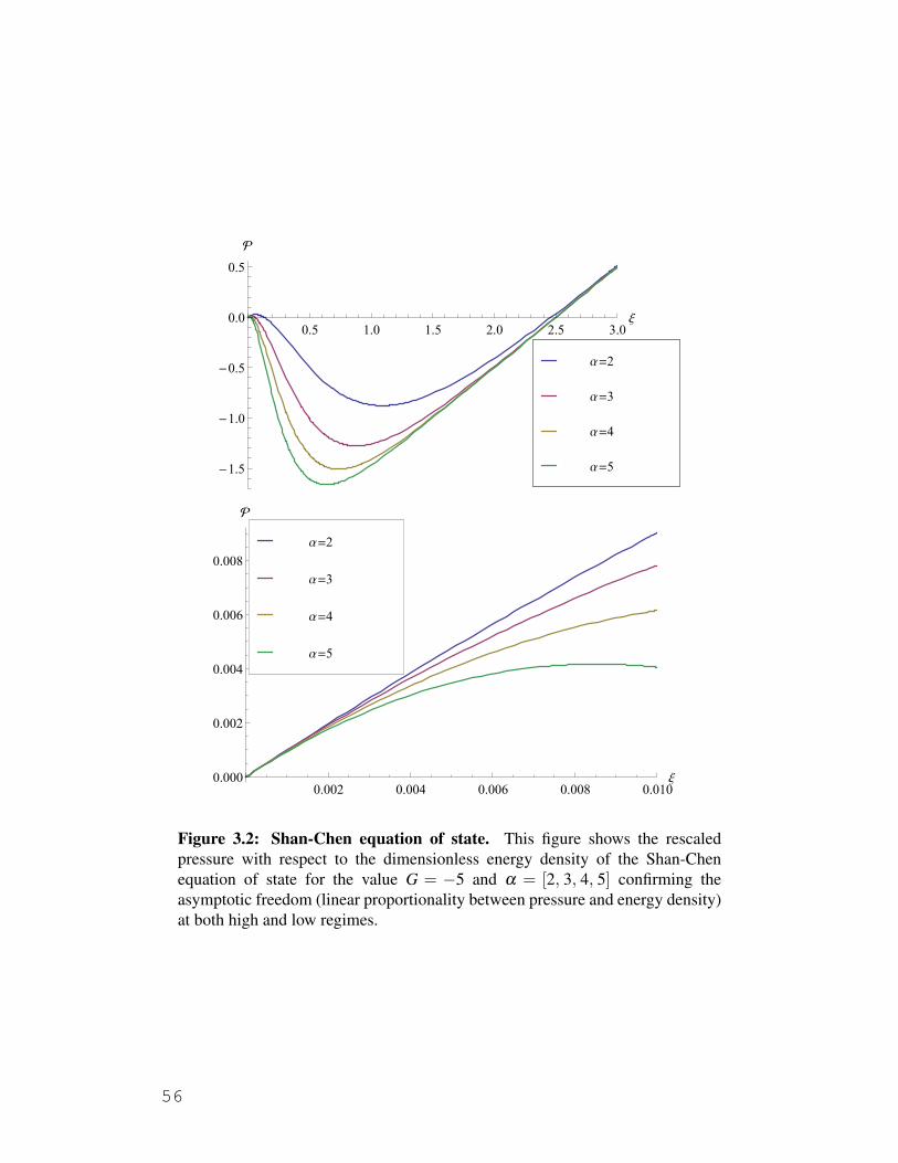
0.5 1.0 1.5 2.0 2.5 3.0

Ξ

-1.5

-1.0

-0.5

0.0

0.5

P

Α=5

Α=4

Α=3

Α=2

0.002 0.004 0.006 0.008 0.010

Ξ0.000

0.002

0.004

0.006

0.008

P

Α=5

Α=4

Α=3

Α=2

Figure 3.2: Shan-Chen equation of state. This figure shows the rescaledpressure with respect to the dimensionless energy density of the Shan-Chenequation of state for the value G = −5 and α = [2, 3, 4, 5] confirming theasymptotic freedom (linear proportionality between pressure and energy density)at both high and low regimes.

56

constant G should be regarded as the bag constant which accounts for thedifference between the energy density of the true vacuum state and theperturbative one. In particular in the parton model of hadrons the authorsreferred to “bag”as the region of space where the strongly interactingfields/particles are confined. Also in this case when the quarks are close toeach other the confining force becomes weaker reaching zero for closeconfinement and consequently the quarks are free to move (anothernon-cosmological application of the idea of asymptotic freedom underlyingthe derivation of the Shan-Chen equation of state) [70].

3.2 Observational tests

In the previous section of the present chapter I have reviewed the derivation ofthe nonideal equation of state of Shan-Chen with asymptotic freedom focusingin particular on the form of the underlying potential and on the fact that it hasbeen proved that it can be used to simulate a liquid-vapor phase transition,phase transition that we expect to appear also when we couple the equation ofstate (3.4) to the Einstein equations (1.5). In this section I will describe how toprove this statement rigorously showing how we can connect the observationaldata collected by the space missions to the quantities entering our theoreticalformulation. The demonstration can be split up into two parts having the aim ofdescribing two completely different stages of the evolution of our Universe: wecan apply the Shan-Chen equation of state to late time cosmology and/or to theinflationary era of the Universe. In both cases the entry and exit mechanismsare crucial for the improvement of the current models.

3.2.1 Late time cosmology

When we apply the Shan-Chen equation of state to the cosmological modelingwe start solving the Friedmann and the energy conservation equations once wehave plugged in this specific equation of state. For the sake of completenessthey are explicitly given by

dξ

dτ= −3

x

dx

dτ

[

(1+w)ξ +w

2G(

1− e−αξ)2]

, (3.11)

dx

dτ= ±

√

Ωk,0 + x2ξ , x =a(t)

a0(3.12)

where τ = H0t, H0 being the Hubble constant, is a dimensionless time and x

is given by the ratio of the scale factor at an arbitrary time a(t) and at todaya0. To find a numerical solution we must then implement the initial conditionsξ (τ0) = Ω0, where Ω0 is the amount of dark energy today, and x(τ0) = 1.

57

We can then plot both the pressure, the energy density and the“effective”parameter of the equation of state weff = P

ξversus the time. The

first important feature of the model is that the pressure as a function of theenergy changes its sign during the time evolution and stays negative for a longtime interval which includes the present day: the physical meaning is that thefluid permeating the Universe naturally and smoothly evolves from anordinary matter content to an energy component whose equation of state iscompatible with dark energy. To have a more realistic picture of the Universewe can consider two non-interacting fluids permeating the Universe which areseparately conserved, namely we add a dust component to the matter contentin terms of a pressure-less fluid. The first basic property of the model, i.e. theevolution from ordinary to dark energy of the Shan-Chen fluid, remains validalso in this extension for another numerical choice of the free parametersentering the equation of state.

From a stricter observational point of view we can compare our model tothe supernova type Ia data, after proving that the Shan-Chen fluid can mimicdark energy. This data set is the first test that a cosmological model mustpass and it is based on the fact that the supernovae are standard candles sincethey exhibit fixed and known luminosity [1; 2]. The test is usually done byplotting the distance modulus with respect to the redshift; the expression forthe distance modulus is [71]

µ = 5logdL

Mpc+25 , (3.13)

where I have inserted the luminosity distance introducing the redshift z

dL = (1+ z)dH

√

|Ωk,0|Σk

(

√

|Ωk,0|dc

dH

)

. (3.14)

dH = 1/H0 is called “Hubble distance“, while dc is the comoving distance andΩk,0 is the curvature parameter, where a subscript here and in what followstates that the quantity is considered at the present time; moreover Σk( f ) =[sin( f ), f , sinh( f )] for a closed, flat and hyperbolic universe respectively. Toobtain the optical properties of the Universe we must integrate the radial nullgeodesic equation in the Friedmann metric dr/dt =−1/a which gives the pathof a light signal moving from a galaxy to us. From this solution we evaluatethen the comoving distance dc = a0r.

In the case of the previously considered ΛCDM model that we want tocompare with, the expression for the comoving distance can be found in [71]:

dc = dH

∫ z

0

dz′

E(z′), (3.15)

E ≡ H

H0=√

ΩΛ,0 +Ωk,0(1+ z)2 +Ωm,0(1+ z)3 .

58

In the formulas above H denotes the Hubble function, ΩΛ,0 and Ωm,0 the massparameters today, where the first accounts for the presence of dark energywhile the latter quantifies the dust; the presence of photons is instead assumedto be negligible. In our original cosmological model, instead, we mustintegrate simultaneously the Friedmann and the energy conservationequations (3.11)-(3.12) and

d

dτ

(

dc

dH

)

= −1

x. (3.16)

The initial condition for the radial coordinate is r(τ0) = 0 which meansdc(τ0) = 0 for the comoving distance. Appropriately choosing the numericalvalues for w, α and G, we have obtained that our curve for the distancemodulus can be exactly superimposed to the ΛCDM one.

As a second test we can plot the Hubble function versus the redshift forthe same choice of parameters as in the previous case: also in this case ourmodel is in agreement with the ΛCDM curve and consequently with theobservational data. This data set has been experimentally obtained exploitingthe aging of passively evolving galaxies (in which there is a negligible starformation activity [72]) [73] and baryon acoustic oscillations [74]. Inparticular the latter ones are density fluctuations of the baryonic matter andare used as a standard ruler in cosmology; they also give information aboutthe large scale structure formation in the Universe.

Finally we have shown the dependence of the deceleration parameter onthe redshift. As I mentioned in the second chapter of this thesis when Idiscussed the inhomogeneous discrete cosmological model, the decelerationparameter is defined through the scale factor and its first and second timederivatives by

q = − aa

a2, (3.17)

where the time dependence of the scale factor is obtained via the Einsteinequations (1.5); its evolution consequently depends on the equation of statewe are dealing with. Our formalism allows us also to evaluate the present dayvalue of the deceleration parameter and the age of the Universe which arecompatible with the observed ones.

Role of instabilities in the hydrodynamic fluid evolution

Even if the theoretical model is compatible with the observational data, asI discussed so far in this section, we are required to do a further check. In factit is important to show explicitly that the model is stable under small initialperturbations, otherwise the mathematical formulation can not be accepted asa description of the physical world. This is a self-consistency exam for the

59

model itself rather than an experimental test. This is because thehydrodynamic approach we followed in the modeling of the matter content ofthe Universe would not hold anymore if it contains growing inhomogeneities,especially under the effect of gravity. Moreover accounting for what Iexplained in the first section of this chapter about the derivation and the basicfeatures of the Shan-Chen equation of state, we know that the hard-corerepulsive effects, which prevent this kind of instabilities in liquids, have nowbeen replaced with soft-core attractive ones with asymptotic freedom: theattractive interactions can consequently facilitate the growth of theinstabilities causing a density blowup and a destruction of the model. In theShan-Chen model the interparticle interaction reaches a saturation valueabove which the interaction strength vanishes; in this specific case theattractive force goes to zero at short distance, or in other words at highdensities. For these reasons a stability analysis of our cosmological modelwas necessary. The study shows that the density contrast defined as the ratiobetween the perturbation of the energy density and the energy density itself isbounded for a long time interval for the same choice of the free parameters inthe equation of state needed for the data fit of the modulus distance and theHubble function versus the redshift, while it explodes only approaching theinitial singularity. In this latter case it is possible to assume without loss ofgenerality that our model is too naive for a complete and correct descriptionof the big bang since we are here interested only in a physical application tolate time cosmology. We also noticed that the presence of a pressure-less fluidcomponent plays a stabilizing role, which was not guaranteed at priori (forexample the Einstein static Universe in which the dark energy is modeled as acosmological constant term rather than a Shan-Chen fluid is unstable [38]).

3.2.2 Inflationary era

So far I have discussed the experimental tests to compare the Shan-Chencosmological model to observations in late time cosmology, however we canexpect that the phase transition exhibited by the fluid during the timeevolution in that context can be employed also for the description of theinflationary era of the Universe, in particular providing a natural exitmechanism from this stage of the evolution of the Universe. This is becausein the standard model of cosmology the dust density dilutes as the volumea3(t), the photons density as a4(t), while the cosmological constant does notdilute at all: when this latter term will become dominant it is impossible toescape from that stage of the evolution. I recall that in the inflationary epochthe Universe undergoes a phase of exponential expansion which is needed tosolve the

60

• flatness paradox: at the present time we observe an almost flat Universe,which requires the Universe to be flat also at the initial moment, if theUniverse is matter or radiation dominated.

• horizon paradox: why do we observe an almost constant temperatureeven in spatial points of the Universe which could not have been incausal contact with each other?

and which has also been proposed in reference to the

• formation of the large scale structure

• origin of the anisotropies in the cosmic microwave background radiation

in the framework of the standard Big Bang model [71; 75].The simplest possible theoretical model for this phenomenon assumes

that the inflationary epoch is dominated by a quintessence fluid which can bedescribed in terms of a real scalar field φ = φ(t), which depends only on thetime for the assumptions of homogeneity and isotropy. The lagrangian isgiven by

L =φ 2

2−V , (3.18)

V =V (φ) being the potential of the field causing the expansion of the Universe.The canonical equations give us the relations between the energy and pressureof the fluid and the field:

ρ =φ 2

2+V , p =

φ 2

2−V , (3.19)

or equivalently

V =1

2(ρ − p) , φ 2 = ρ + p , (3.20)

where in our case we will postulate that the pressure is given by the energy bythe equation of state of Shan-Chen (3.4). We can use this formalism also toconnect the Hubble function to the field obtaining

H2 =1

3

(

φ 2

2+V

)

. (3.21)

This couple of equations shows that the potential driving the inflationary era isfixed when an equation of state is assumed and when the background metricis decided (an extension of the quintessence formalism to a background withsmall inhomogeneities has been considered in the context of the k-essence [8]).

During the inflationary era it is assumed that the kinetic part of thelagrangian (3.18) is negligible respect to its potential part in order to have an

61

exponential growth of the Universe. To define mathematically this conditionwe start introducing the so called slow-roll parameters [71; 75]

ε =1

16π

(

V ′

V

)2

(3.22)

η =1

8π

V ′′

V(3.23)

Ξ =1

64π2

V ′′′V ′

V 2(3.24)

where here a prime denotes derivative with respect to the scalar field φ . Theinflationary era takes place when the above defined slow-roll parameters aresmall:

ε ≪ 1 , |η | ≪ 1 , |Ξ| ≪ 1 , (3.25)

which in particular implies that during this stage the equation of statedescribing the fluid permeating the Universe can be approximated by p ∼−ρ .In the attached paper VII, after deriving the relations between the slow-rollparameters and the energy density of the model we plot the slow-rollparameters as a function of the scalar field φ showing that they respect theconditions required to describe an inflationary scenario for an appropriatechoice of the free parameters of the model. After this initial check we deepenthe connection between the Shan-Chen class of cosmological models and theinflationary paradigm comparing our formalism with the experimental datacharacterizing this era of the Universe. In particular one can consider the ratioof scalar to tensor perturbations, the scalar spectral index and its runningwhich can be expressed in terms of the above defined slow roll parametersfollowing standard literature [75]:

r = 16ε (3.26)

ns = 1−6ε +2η (3.27)

αs =dns

dlnk= 16εη −24ε2 −2Ξ , (3.28)

and consequently as functions of the energy density of the Shan-Chen fluid.The data provided by the Planck mission analyzing the structure of the

cosmic microwave background can be combined with the ones of the largeangle polarization of the Wilkinson Microwave Anisotropy Probe (WMAP) toconstrain observationally these parameters [76; 77]:

r < 0.11 , ns = 0.9603±0.0073 , αs = −0.0134±0.0090 , (3.29)

where in particular the last one suggests that there are no indications for arunning of the spectral index. The spectral index instead comes from the

62

assumption that the power spectrum can be written as a power function whoseexponent is ns −1; its numerical value is fundamental to discriminate betweendifferent proposals of the inflationary mechanism and it is important toobserve that its current experimental value is not compatible with 1 whichcharacterizes gaussian (or adiabatic) initial perturbations [75]. According toour model instead this is not a problem at all since we can reproduce it withinour model.

3.2.3 A word of warning: the BICEP2 experiment

In the previous section I have chosen to use the Planck data, in particular forthe ratio of scalar to tensorial perturbations, for a test of our originalcosmological model. However a recent result by the BICEP2 collaborationsuggests a different observational value for this quantity [78] claiming thedetection of the B-mode. Following the analogy between gravity andelectromagnetism discussed in the second chapter of this thesis, the twopolarizations which could be present in the cosmic microwave backgroundare called E-mode and B-mode, which are respectively the curl-free andgrad-free components. The latter can not be produced only by the physics ofthe plasma (Thomson scattering) and are interpreted as a signal coming fromthe cosmic inflation quantifying the presence of possible primordialgravitational waves. The perturbations in the CMB can then be classified inscalar, vectorial and tensorial with different consequences on the temperatureanisotropies. Looking at the temperature pattern BICEP2 obtains thefollowing quantitative result

r = 0.20+0.07−0.05 , (3.30)

clearly incompatible with Planck’s one

r < 0.11 . (3.31)

At the time of the first submission of paper VII in January 2014 only Planckresults were available justifying my choice of the experimental value tocompare to our Shan-Chen cosmological model.

3.3 Summary

To summarize, in this chapter I have proposed a possible physicalinterpretation of the nature of the dark energy in terms of the nonidealequation of state with asymptotic freedom of Shan-Chen, once I haveassumed that instead the geometric side of the Universe can be well enough

63

described by the Friedmann metric. In this original approach the presence ofthe cosmological constant and of the vacuum energy is not needed foraccounting for many observational data both in the late time cosmology andin the inflationary era. In particular the improvements respect to the previousapproaches are:

• We have understood both the numerical formulation of the equation ofstate describing the fluid permeating the Universe and its theoreticalmeaning; for example this same equation of state can also be applied innuclear physics to the extended model for hadrons. Considering theform of the potential underlying the derivation of this equation of statewe can provide its microscopic interpretation. Thus this is not an ad

hoc formula just derived from the fit of astronomical observations.

• Our model of the Universe exhibits a radiation dominated phase at thebeginning in accordance with the hot big bang model and naturallyevolves to a dark energy dominated one and after we can escape fromthis phase; when the dark energy is modeled as a cosmological constantinstead there are no mechanisms available for such phase transitioninvoking only one fluid.

• We can fit the distant type Ia supernova data with an appropriate choiceof the free parameters appearing in the model without the need of thevacuum energy.

• Our model is also stable under small initial perturbations for the samechoice of parameters that allows us to satisfy the point above; not allthe cosmological models are stable, the Einstein static Universeformulated on the same Friedmann line element like ours and involvinga cosmological constant, a energy density and a pressure is not; ourmodel is thus a step forward also in this direction.

• We have shown that the repulsive action of the cosmological constantcan be handled with an equation of state describing an attractive effectwith asymptotic freedom.

• We can apply our formalism also to describe the inflationary phase ofthe Universe using the quintessence model: we have an exit mechanism.

• In this latter case we can also show the slow-roll conditions to besatisfied and that we can correctly reproduce the numerical values forthe scalar to tensor perturbations, the spectral index and its running.

64

Connecting the first point above with other ones in the list we can say thatwe have suggested a possible microscopic interpretation of the dark energy,interpretation that can also be formulated in terms of a chameleon field. I referto the attached papers V and VII for the details of the derivation of all thestatements claimed here.

65

66

4. Applications of the Poynting-

Robertson effect in general

relativity

4.1 Characterizing a spacetime through the motion of

particles

In the previous chapters of this thesis I have tried to characterize a givenspacetime solving the Einstein equations for the metric after fixing anappropriate matter content of the Universe. A complementary point of view inthe search for the correct modeling of the spacetime consists in the analysis ofthe orbit of a test particle moving inside it. The first step in this direction isthe analysis of the geodesic motion, a purely geometric effect which dependson the metric and its first derivatives (the Christoffel symbols): setting theacceleration equal to zero the mass of the body drops out and we distinguishonly between the cases of massive or massless test particles. The gravitationaleffects on a particle motion are therefore encoded inside the line elementwhich is coupled to the matter distribution via the Einstein equations. Thusaccording to general relativity the test particle interacts with the matterthrough this process; reversing this point of view we can reconstruct someproperties of the metric and consequently of the matter distribution generatingit following the motion of a particle. We can refer to this phenomenon as akind of indirect interaction between test particle and matter.

To obtain a more accurate picture of the matter content in the regioncrossed by our test particle we should also consider its direct interaction withthe fluid. In fact we can suppose that during its motion the body collides withthe fluid elements exchanging energy with them. Assuming that the energy istransferred from the object to the matter content, the fluid acts as a viscousmedium leading to the presence of a dissipative force term inside theequations of motion. In classical mechanics the expression for such a frictioneffect is modeled by the Stokes’ law, which can be extended to generalrelativity using the Poynting-Robertson formula as I proved in section (1.5) ofthis thesis. Moreover the general relativistic formalism that I will follow in

67

this chapter can describe both the case of motion inside a massive or massless(photons) fluids that instead was not possible in the classical treatment.

We can also distinguish between two more approaches to this problem.In the first one a background is fixed and described by the metric gµν andwe superpose to it a test fluid whose stress-energy tensor is a function of thisbackground:

Tµν = (ρ + p)uµuν + pgµν , (4.1)

ρ and p being its pressure and density energy connected to each other by aspecific equation of state, while uµ denotes the fluid four-velocity. Thisexpression shows that the formalism is enough general to describe both thecases of massive or massless media. The quantity (4.1) is the stress-energytensor which enters the Poynting-Robertson formula that I recall here for thesake of completeness

f(fric)(U)α = −σP(U)αβ T β µUµ . (4.2)

In the formula above the sign minus accounts for the dissipative nature of theforce, the cross section of the process σ contains the details of theinteractions between test particle and fluid, Uµ is the body four-velocity andP(U)α

β projects orthogonally to this four-velocity. In a first attempt we canconsider the weak field approximation assuming that the fluid field does notperturb the spacetime. The derivation of the expression of the stress-energytensor for a fluid placed in a curved background can also be seen as aninteresting application of the kinetic theory and of the Boltzmann equation ingeneral relativity [79]. We have followed this procedure in particular in paperI studying the motion of a massive object around a Schwarzschild black holeto which we superpose a test photon field comparing and contrasting thegeodesic and scattered motions. Our original analysis was necessary for theclarification of the role of friction and of radiative pressure in thePoynting-Robertson formula [80; 81]. The literature is rich of examples ofthis kind of applications: from the motion of meteors to the modeling of anaccretion disk around a star due to this phenomenon [82–84].

The first question which arises at this point is: how good is theapproximation of a test field for the photon gas? Can the motion of the testparticle deviate also qualitatively and not only quantitatively when we leavethis regime? To answer this question we must solve the Einstein equation(1.5) to describe a system of a black hole surrounded by a photon gas. Thisanalytical solution is not known yet. Thus we have decided to “switch off”theblack hole and to consider a spacetime generated by a photon gas inequilibrium. The Tolman metric is the solution of the field equation in thiscase [85]. Inserting the same stress-energy tensor in both the Einstein

68

equations and the Poynting-Robertson formula (4.2) we can compare andcontrast the geodesic and the modified motions in the Tolman spacetime. Thegeodesic case is what we have called the “indirect”interaction between testparticle and fluid, while the scattered motion accounts also for the“direct”interactions. The analysis allows us to separate the role of thecurvature of the spacetime to the true friction effects inside this phenomenon.This is the subject of paper II. The analysis can also be compared to a similarone in the Vaydia metric which instead mimics a photon field not inequilibrium like a radiating star [86].

In paper III we have extended the Poynting-Robertson formula, which wasinitially proposed for the motion inside a massless fluid, to the motion inside amassive fluid. In fact there can be gas clouds in the Universe which distort theorbits of particles crossing them acting as a gravitational lensing. The goal ofthis specific analysis is the evaluation of the deflection angle which quantifiesthe difference between the case of a particle moving in vacuum and a particletraveling this region. Also in this case the geodesic and non-geodesic casescan be compared and we have proved that when we add a viscous term to theequations of motion the body can not escape the gas cloud once it has enteredit because it dissipates all its initial energy and it is consequently condemned tofall at the center of the configuration. The friction effects are thus much moreimportant than the space curvature ones. To be specific, for this derivation wehave considered the Pant-Sah metric as a background.

In the cosmological modeling our formalism can be applied to thequantification of the peculiar velocities, which is the motion of a particle withrespect to an observer in a rest frame. In paper IV we have considered aFriedmann expanding Universe whose matter source driving its evolutioninfluences also the friction force (4.2). In this case when we add thePoynting-Robertson formula to the geodesic equation of motion we cantherefore speak of direct interaction between the test particle and the fluid. Inthe case of a closed Universe the asymptotic behavior of a particle movinggeodesically and geodesically plus friction is completely different: in theformer the object accelerates to the speed of light, while in the latter itdissipates all its initial energy approaching zero velocity. As for the previousanalysis of the gravitational lensing, the friction term plays a fundamentalrole in driving the long-term result and should not be neglected in a realisticmodeling of the motion.

In this chapter I will review all these astrophysical applications of thePoynting-Robertson formula leaving the details of the complete derivation tothe attached papers at the end of the thesis and [46; 47; 80–84] and referencestherein. I would like to stress that in this analysis we have assumed that all thenoise effects are negligible even if they should be accounted by the

69

relaxation-dissipation theorem: this opens a line for future possibleinvestigations which will provide a more complete picture of thisphenomenon. Our formalism is also enough general to be applied to nonastrophysical systems in which friction effects anyway occur.

4.2 Motion inside a photon gas in the Schwarzschild

metric

In this section I am interested in describing the motion of a massive testparticle around a Schwarzschild black hole to which I have superimposed atest photon gas (the strength of the field is sufficiently weak not to perturb thefixed background metric). The first task is consequently to derive thestress-energy tensor describing such a gas in a curved spacetime and theninsert it inside the Poynting-Robertson formula (4.2). This can be seen as anapplication of the relativistic kinetic theory in a generic curved spacetime.

We can follow for example [87]. I start from a generic line element

ds2 = gαβ dxαdxβ . (4.3)

Assuming then that all the particles of the gas are indistinguishable with thesame mass m, which can be set equal to zero at the end of the computationswithout problems, we have the following constraint in the momentum space:

pµ pµ = −m2 , (4.4)

where pµ is the four-momentum of the particles. Introducing the phase space,the gas is characterized by the distribution function f (xµ , pµ), xµ denoting thecoordinates in the real space, whose evolution can be followed along a lineparameterized by τ :

d

dτf (xµ(τ), pµ(τ)) =

∂ f

∂xµ

dxµ

dτ+

∂ f

∂ pµ

d pµ

dτ. (4.5)

This relation reduces to the homogeneous relativistic Boltzmann equation

L( f ) =

(

pµ ∂

∂xµ−Γµ

αβ pα pβ ∂

∂ pµ

)

f = 0, (4.6)

where L is referred to in the literature as the Liouville operator, in the case thatthe gas particles interact only gravitationally moving along geodesics

d pµ

dτ= −Γµ

αβ pα pβ . (4.7)

70

Generalizing the previous result accounting for the collisions between the gasmolecules, assumed to be elastic (the total four-momentum is conserved) andbinary, we obtain

L( f )(xµ , pµ) =∫

Cd4 pd4qd4q, (4.8)

where I have introduced

C ≡ C( f ;xµ , pµ , qµ , pµ ,qµ) = ω[ f (xµ , pµ) f (xµ , qµ)− f (xµ , pµ) f (xµ ,qµ)],(4.9)

where ω = ω(xµ ; pµ , qµ , pµ ,qµ) represents the phenomenological crosssection of the process; here xµ denotes the point in the physical space wherethe collision takes place and pµ , qµ , pµ , qµ the four-momenta of the collidingparticles before and after the collision. Summarizing, the collision integraldescribes the variation rate of the number of particles in a given region of thephase space [68].

The physical properties of the gas considered are contained in the momentaof the distribution function: the current of particles density, the stress-energytensor and the current of entropy density:

Nµ =∫

f 2δ+(p2 +m2) pµ

√−gd4 p

(2π)3=∫

fpµ

|pt |

√−gd3 p

(2π)3(4.10)

T µν =∫

f 2δ+(p2 +m2) pµ pν

√−gd4 p

(2π)3=∫

fpµ pν

|pt |

√−gd3 p

(2π)3

Sµ = −kB

∫

( f ln f )pµ

|pt |

√−gd3 p

(2π)3,

where g is the determinant of the background metric and kB the Boltzmannconstant. It can be proved by direct inspection that in a generic spacetime thesolution of the collisional relativistic Boltzmann equation is given byf = αeβξµ pµ

, ξµ being a timelike Killing vector of the background metric, α

a normalization constant and β = 1/kBT the inverse temperature. In thespecific case of the Schwarzschild spacetime such Killing vector isξµ = (∂t)µ . For the explicit evaluation of the statistical momenta, thefunctional generator technique

Nµ =1

β

∂ I

∂ξµ(4.11)

T µν =1

β 2

∂ 2I

∂ξµ∂ξν=

1

β

∂Nµ

∂ξν(4.12)

Sµ = −kB

∫

( f ln f )pµ

|pt |d3 p

(2π)3= −kB

[

ln(α)Nµ +∂Nµ

∂ξνξν

]

,(4.13)

71

where I have introduced

I =∫

f (ξµ pµ)2δ+(p2 +m2)√−gd4 p , (4.14)

is of great help. After some algebraic manipulations [79], the stress-energytensor for a massless gas in a curved spacetime is reduced to

Tµν = (ρ + p)uµuν + pgµν =C

3(βξ )4[gµν +4uµuν ] , (4.15)

where uµ =ξµ

ξis a unit vector where ξ =

√

−ξµξ µ . In equation (4.15) wehave reobtained in a more formal way both the expected equation of state fora photon system p = 1

3 ρ , and the Tolman law β → βξ for the temperature.

Finally the constant C = π2

15 has been determined requiring to be in agreementwith the black body theory in a flat spacetime. Direct inspection of theexpression (4.15) shows that the conservation law T µν

;µ = 0 and the tracefreecondition of an radiation field T µ

µ = 0 hold.Considering a Schwarzschild spacetime

ds2 = −N2dt2 +1

N2dr2 + r2dθ 2 + r2 sin2 θdφ 2 , N = N(r) =

√

1− 2M

r,

(4.16)M denoting the mass of the central black hole, then the explicit expression forthe Poynting-Robertson formula (4.2) is reduced to

f (U)αrad = −mA

N4γ3[ν2uα +να ] , (4.17)

after inserting the stress-energy tensor (4.15). In this expression m is the massof the test particle moving inside the photon gas around the black hole, A aconstant of proportionality containing information about the temperature ofthe photons, the cross section of the process, and other numerical constants, γ

is the Lorentz factor and να the spatial part of the test particle four-velocity(1.22).

I recall that the equation of motion are given by the superposition of thegeodesic part and of the friction term:

mUβ ∇βUα = f (U)αrad . (4.18)

Numerically integrating this set of equations we observed that:

• The motion is still planar as in the pure geodesic case.

72

• Considering as initial condition the circular geodesic orbit for a puregeodesic case with r = 4M and νK = 1√

2, here νK being the keplerian

velocity, the test particle falls inside the black hole crossing its horizon.Thus the circular motion is modified to a spiral one. This behavior canbe understood in terms of the physical nature of thePoynting-Robertson formula: it is a friction effect and consequently thetest particle is condemned to dissipate its initial energy.

• Our analysis can be compared to a previous one in which the stress-energy tensor for a null dust around a Schwarzschild black hole waswritten as

T µν = Φ2kµkν , kµkµ = 0 , (4.19)

where kµ is a vector tangent to a null geodesic, while Φ is a functionto be determined imposing the conservation law T µν

;µ = 0 in a specificspacetime. In this previous analysis the null dust acts as a wind andthe test particle, whose motion is based on the same initial condition asin the point above, reaches an equilibrium point (outside the horizon)where the gravitational attraction of the black hole equates the radiativepressure of the field.

• Our original result based on a statistical modeling of the photon gas wasfundamental in separating the two parts, the radiation pressure and thefriction term inside the Poynting-Robertson effect.

• According to our analysis the Poynting-Robertson effect can play somerole in the formation of an accretion disk in the vicinity of a star or ablack hole because the test particle stops its motion closer to the horizonthan the innermost stable geodesic circular orbit (classical description ofthe photons moving along a preferred direction), or crosses it (originalapproach).

I would like to mention that I started studying the topic presented in this sectionwith my master thesis [88], but it has been completed only during my Ph.d. Inthe future this same analysis should be extended to a rotating Kerr black hole.

4.3 Metric curvature versus friction effects

In the previous section the photons were considered as a test field which doesnot perturb the Schwarzschild black hole. However also the strong limit caseis physically interesting. To study a configuration in which the presence of thephotons models the spacetime, we have eliminated the black hole and on theother hand we have solved the Einstein equation (1.5) for a photon system in

73

gravitational equilibrium as a matter source. Since the gas is assumed to be inequilibrium the metric must be spherically symmetric and we can start fromthe ansatz

ds2 = −eν(r)dt2 +

(

1− 2M(r)

dr

)

dr2 + r2dθ 2 + r2 sin2 θdφ 2 . (4.20)

Its explicit expression can be derived using the Tolman-Oppenheimer-Volkoffformalism once a specific matter content is assumed. The TOV set of equationsare given by [89; 90]:

d p(r)

dr= − 1

r2(ρ(r)+ p(r))(M(r)+4πr3 p(r))

(

1− 2M(r)

r

)−1

(4.21)

dM(r)

dr= 4πρ(r)r2

dν(r)

dr= − 2

ρ(r)+ p(r)

d p(r)

dr.

In this set of equations p(r) and ρ(r) are the pressure and the energy density ofthe fluid function only of the radial coordinate and related to each other by anequation of state which reflects the fluid we are considering, while M(r) canbe regarded as the mass of the configuration inside a sphere of radius r. In thecase under examination we choose p(r) = 1

3 ρ(r) and the Tolman metric givesthe solution we are looking for [85]:

ds2 = −ardt2 +1

adr2 + r2(dθ 2 + sin2 θdφ 2) , a =

4

7, (4.22)

and the energy density

ρ =3

56πr2, (4.23)

is in agreement with the Tolman law for static spacetime [91]. Three featuresof the line element (4.22) are evident:

• The energy density approaches zero as a function of the radial coordinateonly asymptotically: we can not have a bounded photons configurationin equilibrium from which photons can not escape otherwise we willhave a black hole.

• The metric exhibits a naked singularity in the point r = 0 as it comesfrom the evaluation of the Kretschmann scalar

K = Rαβγδ Rαβγδ ∼ 1

r4. (4.24)

74

• The metric describes a photon gas configuration in equilibrium and nota radiating star (it is static) and consequently its form is completelydifferent from the Vaidya metric [86]

ds2 = −(

1− 2M(v)

r

)

dv2 +2dvdr + r2(dθ 2 + sin2 θdφ 2) . (4.25)

To quantify the relative importance between spacetime curvature and frictionterm in the modeling of the Poynting-Robertson effect three different situationsfor the motion of a massive test particle must be compared:

• We consider a test photon field superimposed to a fixed Minkowskibackground: only friction effect, no curvature (being the Riemanntensor identically zero).

• We consider a geodesic motion inside the Tolman metric (4.22): onlycurvature, no friction; we can refer to this case as an indirect interactionbetween test particle and photon gas through the Einstein field equations.

• We consider a Poynting-Robertson effect in the Tolman metric: bothfriction and curvature of the space are accounted for; in this case there isa direct interaction between the test particle and the fluid generating thespace since there are collisions between them (which microscopicallycan be regarded as a Thomson scattering).

I would like to mention that the analysis of the motion of a particle in sucha metric should not be considered only as a theoretical exercise because theTolman metric can also describe a static Universe radiation dominated. Thecharacteristics of the motion are the following.

• Only friction, no curvature: the massive test particle moves along astraight line, as in the case of Minkowski metric without thePoynting-Robertson term, but decelerating and reaching a motionendpoint with zero speed. As in the classical mechanics counterpart inwhich the friction force is given by the Stokes’ law, the velocity isexponentially decaying. On the other hand we have observed that in arelativistic context, contrary to the newtonian one, the object crosses amaximum distance independently of its initial speed:

dmax =π

2A, A =

4ρ0σ

3m, (4.26)

where ρ0 is the constant energy density of the photon gas, σ the crosssection of the process appearing in the Poynting-Robertson formula

75

(4.2), while m is the mass of the test particle. The quantity A cantherefore be interpreted as an effective coupling constant between testparticle and field which quantifies the energy absorption andre-emission from the photons. The upper limit stated above opens thequestion if a similar condition holds also in a curved spacetime inwhich the energy of the photon gas is not anymore constant but goes tozero asymptotically with r (4.23).

• Only curvature, no friction: considering a geodesic motion in theTolman metric, the test particle orbit is bounded between two specificvalues of the radial coordinate whose numerical values depend on theinitial condition of the motion. The radial coordinate plotted as afunction of the proper time exhibits an oscillating behavior.

• Curvature plus friction: in this case the massive test particle reaches thecenter of the configuration following a spiral with vanishing speed forall the numerical tests analyzed. The speed of the test particle shown interms of the proper time exhibits a damped oscillating behavior.

To summarize we have showed that in this specific spacetime the frictiondominates over the curvature because asymptotically the massive object stopsits motion, as in the case in which the curvature non-linearities were sent tozero. The assumption of test field for the photons consequently does notinfluence the long-time modeling of the motion. A stronger analytical proofof this claim opens a direction for future possible research.

4.4 Extending the Poynting-Robertson formalism to

the case of a massive fluid

In this section I will report about the results of the second part of the attachedpaper III; the first part has already been discussed in section (1.5) where theextension of the Poynting-Robertson formula from the motion inside amassless gas to the motion inside a massive fluid has been derived. Thisproves that their formalism is the correct general relativistic counterpart of theStokes’ law. I will focus here instead on the physical application of thisinterpretation studying the motion of a body inside a massive gas cloudformally described by the exact Pant-Sah solution of the Einstein equations.Thus I start reviewing how the solutions of the field equations have beenconstructed in general relativity to describe a system of self-gravitatingparticles in equilibrium [89; 90; 92; 93; 95–97]; in particular I will followclosely [94] since this set of solutions received poor attention in literature so

76

far. In this latter paper the authors start from the general form of the lineelement in isotropic coordinates for a spherically symmetric system:

ds2 = −eν(r)dt2 + eω(r)(dr2 + r2dθ 2 + r2 sin2 θdφ 2) , (4.27)

and the well-known expression for the stress-energy tensor as function of theenergy density and pressure of the fluid:

T tt = −ρ , T r

r = T θθ = T φ

φ = p . (4.28)

Then Pant and Sah have proved that the Einstein equations for such a systemare reduced to:

8π p = e−ω

[

ω ′2

4+

ω ′

r+

ω ′ν ′

2+

ν ′

r

]

(4.29)

8π p = e−ω

[

ω ′′

2+

ν ′′

2+

ν ′2

4+

ω ′

2r+

ν ′

2r

]

(4.30)

8πρ = −e−ω

[

ω ′′ +ω ′2

4+2

ω ′

r

]

, (4.31)

where a prime denotes, as usual, derivative with respect to r. The first twoequations of the system above can be combined together to give:

ν ′′ +ω ′′ +ν ′2

2− ω ′2

2−ν ′ω ′− 1

r(ν ′ +ω ′) = 0 , (4.32)

which admits the solution

eν2 = A

1− kδ

1+ kδ, e

ω2 =

(1+ kδ )2

1+ r2

a2

, (4.33)

where

δ = δ (r) =

(

1+ r2

a2

)12

(

1+b r2

a2

)12

, (4.34)

with A, a, b and k numerical constants. This is exactly the procedure followedby Pant and Sah for deriving their namesake solution. The pressure and energydensity can then be expressed in terms of this set of quantities as

8π p =4(bk2δ 6 −1)

a2(1+ kδ )5(1− kδ )(4.35)

8πρ =12(1+bkδ 5)

a2(1+ kδ )5, (4.36)

77

which are consequently connected by the equation of state

p = p(r) =ρ

65

1+2qc(1−ρ15 )

, a =2qc

1+qc

, (4.37)

which should be regarded as a generalized polytropic equation of state of indexn = 5. The sound speed for such a system is:

cs =

√

∂ p

∂ρ=

p

ρ

√

2

5ρ15

(3+6qc −5qcρ15 ) . (4.38)

This last expression motivates why the Pant-Sah solutions have been lookedfor: they are more realistic than the interior Schwarzschild solution (whichcan be derived from the Tolman-Oppheneimer-Volkoff equations (4.21) for asphere of constant density everywhere):

ds2 = −N21 dt2 +

dr2

N22

+ r2(dθ 2 + sin2 θdφ 2) (4.39)

N1 ≡ N1(r) =3

2

√

1− 2M

R− 1

2

√

1− 2Mr2

R3, N2 ≡ N2(r) =

√

1− 2Mr2

R3,

M denoting the total mass of the configuration, to have a system in which thesound speed assumes physical values. I would like also to mention that theparticular case for which b = 0, implying that

δBuchdahl =

√

1+r2

a2, (4.40)

is referred to in the literature as the Buchdahl solution.Figures (4.1)-(4.2)-(4.3) picture what I have explained so far in this section.

The first two plots show the equation of state p as a function of ρ and the soundspeed versus the energy density for the set of values a = [0.1, 1.0, 1.4, 1.5].The third instead gives an estimate of the radius of the configuration for thespecific values k = 4, a = 1.5 and b = [0.010, 0.050, 0.000, −0.002], wherethe first two numerical values of b correspond to bounded Pant-Sah solution,the third to the unbounded Buchdahl solution and the fourth to the unboundedPant-Sah solution.

Moreover it is important to stress that the case b > 0 describes a finiteboundary fluid distribution, while b ≤ 0 (being the Buchdahl one part of thissecond class) models unbounded distributions. Thus if we would like tointerpret the Pant-Sah solution as a modeling of an astrophysical gravitationallensing we must restrict ourselves to the former case. Literature also explains

78

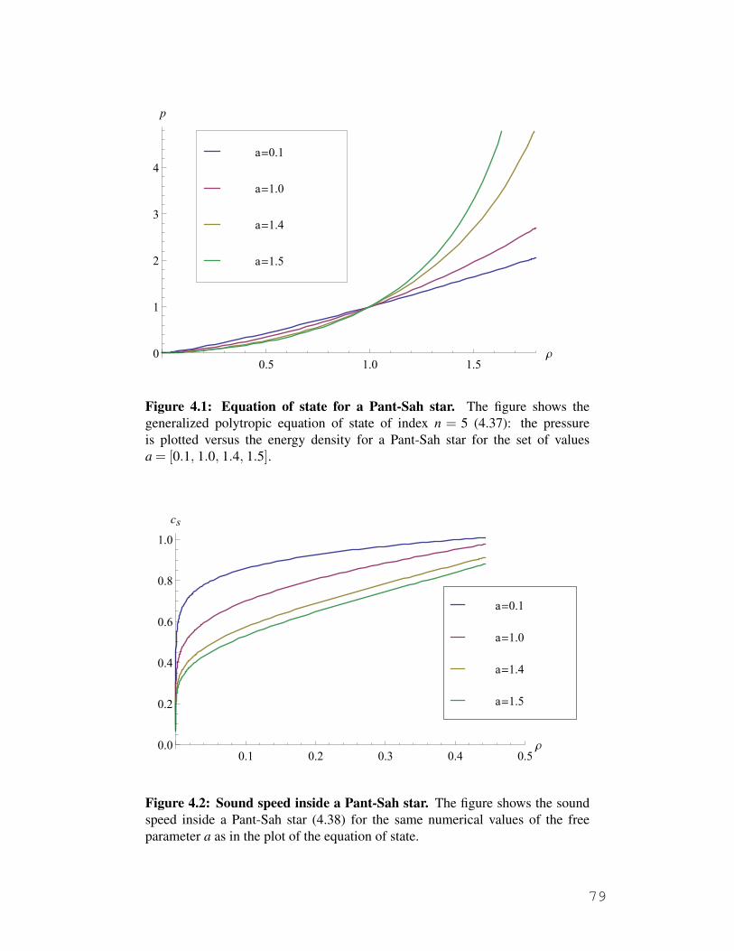
0.5 1.0 1.5

Ρ0

1

2

3

4

p

a=1.5

a=1.4

a=1.0

a=0.1

Figure 4.1: Equation of state for a Pant-Sah star. The figure shows thegeneralized polytropic equation of state of index n = 5 (4.37): the pressureis plotted versus the energy density for a Pant-Sah star for the set of valuesa = [0.1, 1.0, 1.4, 1.5].

0.1 0.2 0.3 0.4 0.5

Ρ0.0

0.2

0.4

0.6

0.8

1.0

cs

a=1.5

a=1.4

a=1.0

a=0.1

Figure 4.2: Sound speed inside a Pant-Sah star. The figure shows the soundspeed inside a Pant-Sah star (4.38) for the same numerical values of the freeparameter a as in the plot of the equation of state.

79

0.5 1.0 1.5 2.0 2.5 3.0

r

-0.00001

-5.´ 10-6

0

5.´ 10-6

0.00001

p

b=-0.002

b=0.000

b=0.050

b=0.010

Figure 4.3: Radius for a Pant-Sah star. The figure shows the pressure in termsof the radial coordinate (4.35) for a Pant-Sah star for the values k = 4, a = 1.5 anda set of values for b. The case b = 0.000 corresponds to the Buchdahl solution inwhich the pressure approaches zero only asymptotically. For b = 0.010 and b =0.050 the radius of the configuration is given by the value at which the pressureswitches its sign. Moreover it can be noted that p is a monotonically decreasingfunction of the distance from the center of the star, as expected.

80

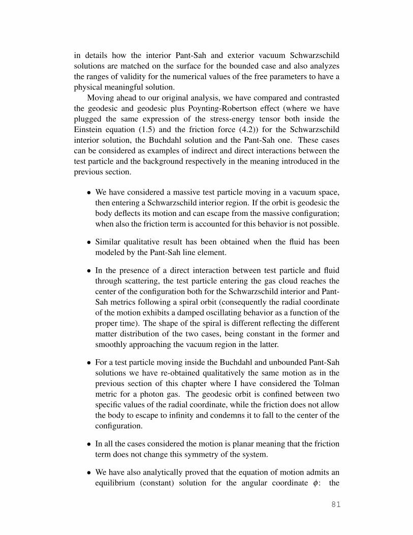
in details how the interior Pant-Sah and exterior vacuum Schwarzschildsolutions are matched on the surface for the bounded case and also analyzesthe ranges of validity for the numerical values of the free parameters to have aphysical meaningful solution.

Moving ahead to our original analysis, we have compared and contrastedthe geodesic and geodesic plus Poynting-Robertson effect (where we haveplugged the same expression of the stress-energy tensor both inside theEinstein equation (1.5) and the friction force (4.2)) for the Schwarzschildinterior solution, the Buchdahl solution and the Pant-Sah one. These casescan be considered as examples of indirect and direct interactions between thetest particle and the background respectively in the meaning introduced in theprevious section.

• We have considered a massive test particle moving in a vacuum space,then entering a Schwarzschild interior region. If the orbit is geodesic thebody deflects its motion and can escape from the massive configuration;when also the friction term is accounted for this behavior is not possible.

• Similar qualitative result has been obtained when the fluid has beenmodeled by the Pant-Sah line element.

• In the presence of a direct interaction between test particle and fluidthrough scattering, the test particle entering the gas cloud reaches thecenter of the configuration both for the Schwarzschild interior and Pant-Sah metrics following a spiral orbit (consequently the radial coordinateof the motion exhibits a damped oscillating behavior as a function of theproper time). The shape of the spiral is different reflecting the differentmatter distribution of the two cases, being constant in the former andsmoothly approaching the vacuum region in the latter.

• For a test particle moving inside the Buchdahl and unbounded Pant-Sahsolutions we have re-obtained qualitatively the same motion as in theprevious section of this chapter where I have considered the Tolmanmetric for a photon gas. The geodesic orbit is confined between twospecific values of the radial coordinate, while the friction does not allowthe body to escape to infinity and condemns it to fall to the center of theconfiguration.

• In all the cases considered the motion is planar meaning that the frictionterm does not change this symmetry of the system.

• We have also analytically proved that the equation of motion admits anequilibrium (constant) solution for the angular coordinate φ : the

81

presence of a gravitational lensing along the path of an object does notnecessarily distort its motion.

I would like to conclude this section recalling that evaluating the angulardistortion for the orbit of the test particle in terms of the radial distance fromthe center of a cluster of galaxies, we can reconstruct the mass of thisself-gravitating system [98; 99]. Moreover the evaluation of the observationaldistortion can also provide an indirect estimate for the coupling constantbetween the test particle and the background fluid.

4.5 Peculiar velocities in astrophysics

The formalism used in the previous sections of this chapter for the descriptionof the motion of an object inside a gas cloud can be extended to the case of anexpanding or contracting spacetime, like the Friedmann one (1.8) aboutwhich I have spoken in the third chapter of this thesis in the framework of theconstruction of an original class of cosmological models. Thus this section ismeant to deepen the understanding of the concordance model of cosmologyconsidering the motion of a galaxy inside a homogeneous and isotropicUniverse when its direct interaction with the intergalactic medium isaccounted for. The motivation for this study is that the search for the correctmodel for our Universe is a hot matter of debate in the context of generalrelativity and the motion of a galaxy strongly depends on the description ofthe relativistic spacetime. A complementary analysis about peculiar velocitiesand matter horizons has recently been discussed in [100]

The explicit form of the Poynting-Robertson formula (4.2) is in this casegiven by

f (U)rad = −σ(1+w)γ2ρνU , (4.41)

where σ is as usual the cross section of process, w = pρ describes a

one-parameter polytropic equation of state for the fluid driving the dynamicsof the Universe (we have assumed the presence of only one mattercomponent), p and ρ being its pressure and energy density respectively; γ

represents the dilation Lorentz factor, ν the magnitude of the spatialcomponent of the test particle four-velocity and finally U is a spacelike vectororthogonal to U in the plane of motion. It is interesting to note that in theexotic case of dark energy the motion reduces to a purely geodesic onebecause of the vanishing of the r.h.s of equation (4.41).

82

The system of equation to be integrated can be shown to reduce to

ν = −ν

γ

[

A(1+w)ρ +1

γ

a

a

]

,

α =νΣ′ cosα

aΣ, r =

ν sinα

a, φ =

ν cosα

aΣ,

a =

√

−k +8

3πρa2 , (4.42)

where α is the inclination of the motion, A = 8πσm

the effective couplingconstant between test particle and field, while k and Σ have been defined insection (1.2) of this thesis. The energy density depends on the scale factor ofthe Universe as in the concordance model of cosmology:

ρ = ρ0

(a0

a

)3(1+w), (4.43)

where ρ0 and a0 are the initial values for the energy density and the scalefactor respectively. I have presented explicitly this system of equation toexplain what I mean by direct interaction between test particle and field: thespacetime is evolving (equation for the scale factor) because of the presenceof a time-dependent energy density; this same energy density appearsexplicitly also in the equation for the evolution of the magnitude of the spatialvelocity of the particle (it enters only indirectly the equation for theinclination). The equations governing the time evolution of the scale factorand the velocity must consequently be integrated simultaneously.

The first equation of the system (4.42) enlightens also the two separatecontributions in the spatial acceleration, the friction and gravitational ones:

ν = a(fric) +a(grav) , (4.44)

with

a(fric) = −A(1+w)ρν

γ, a(grav) = − ν

γ2

a

a, (4.45)

whose ratio can be considered as a function of time to evaluate which one isdominant in the different epochs of the Universe. In particular the friction termwill always decelerate the test particle, while the gravitational one can alsoaccelerates it during the re-collapsing phase of a closed Friedmann Universe.

According to our analysis, the motion exhibits the followingcharacteristics:

• The motion is radial for all the cases of hyperbolic, closed and flatUniverse.

83

• Hyperbolic Universe: the test particle velocity is approaching zero bothin the pure geodesic (A = 0 in the system of equations (4.42)) andgeodesic plus Poynting-Robertson effect cases. The friction effects thusplay a more minor role than in the case of a closed Universe.

• Flat Universe: qualitatively the same behavior as for the hyperbolicUniverse.

• Closed Universe: the motion undergoing friction effects radicallydeviates from the geodesic one; in the latter case the test particlereturns to the ultrarelativistic equilibrium limit for the velocity ν → 1,as expected from the big crunch model, while in the former goes tozero. This is true because in the recollapsing phase of the Universe theenergy density increases causing a dominant effect of the frictiondeceleration versus the gravitational (positive) acceleration.

• Our formalism does not allow us to discriminate between differentequations of state for the fluid permeating the Universe because of thegreat ignorance inside the modeling of the effective coupling constantbetween test particle and field (namely inside the cross section of theprocess σ whose value must be sharply refined in a possible futureextension of this work).

The analysis of this section could be applied to deepen our knowledge of thestandard model of cosmology as follows. I begin introducing thetime-dependent proper distance between an observer and a galaxy D = ar

where r indicates the matter comoving radial coordinate and a = a(t) thescale factor at a specific instant. The so-called coordinate velocity betweengalaxy and observer is then derived from the Hubble law v = D = ar = HD,where I have introduced the Hubble function H = a

a[31]. In our case instead

also r depends on the time t with the matter non comoving, implying that theHubble law should be modified as v = HD+ν , where I have explained in thissection how to determine quantitatively the contribution of ν . The observedastronomical structures consequently deviate from the Hubble motion and areexpected to approach it only as a limiting case. It is expected that future spacemissions will quantify experimentally the deviation theoretically derived here[101; 102] increasing our knowledge of the line element of the Universe andits matter content.

To summarize, in this chapter I have dealt with the scattered motion of amassive body in a given spacetime undergoing geodesic plus friction effects.

84

This latter term has been modeled a la Poynting-Robertson. Both the cases ofmotion in static and non-static spacetimes have been treated, as well as themotion inside a viscous massless (for which the formalism we followed wasinitially proposed in the standard literature) or massive medium. Physicalapplications have been discussed to the modeling of the formation of anaccretion disk around a star, motion distorted by a gravitational lensing andastrophysical peculiar velocities. A possible future analysis requires theextension of such formalism to other contexts in which friction has beenneglected so far: we want to move from the indirect interaction between testparticle and fluid contained in the geodesic equation to the direct interaction(collisions between test particle and fluid generating the spacetime). Also itsmore realistic modeling accounting for the noise effects will be addressed infuture. The technicalities of the derivation of all the results briefly presentedin this chapter can be found in the attached papers I, II, III and IV at the endof this thesis.

85

86

Sammanfattning

Denna avhandling behandlar de öppna frågorna att ge en kosmologisk modellsom beskriver ett accelererat expanderande universum utan att bryta motenergivillkoren eller en modell som bidrar till den fysikaliska tolkningen avden mörka energin. Det första fallet analyseras med hjälpav en sluten modellbaserad på ett regelbundet gitter av svarta hål med användning av Einsteinsekvation i vakuum. I det senare fallet kommer jag att förbinda den mörkaenergin med Shan-Chens tillståndsekvation. En jämförelse mellan dessa tvåförslag diskuteras därefter. Som ett kompletterande ämne diskuterar jagrörelse av testpartiklar som i en allmänrelativistisk rumtid genomgårfriktionseffekter. Detta är modellerat efter Poynting-Robertsons formalism,vars koppling till Stokes formel presenteras. Fallen av geodetisk ochicke-geodetisk rörelse jämförs och kontrasteras för metrikerna Schwarzschild,Tolman, Pant-Sah och Friedmann respektive.

Acknowledgements

In this page I would like to thank the people without whose support I wouldhave never achieved this goal.

Innanzitutto la mia famiglia: un sentito grazie ai miei genitori Patrizia eDario e a mio fratello Paolo per la loro continua presenza in questi anni didottorato e ai miei nonni, in particolare Bepi, per avermi sempre incoraggiatonell’intraprendere tali studi.

It would have never been possible to me to write my thesis without thehelp and the advice of my supervisor Kjell: I thank you for accepting me asa student inside your working group, for correcting my numerous mistakeswith endless patience and for visiting me in Potsdam in November 2012 andin February 2014.

I would like to thank the founder and director of the International Centerfor Relativistic Astrophysics Network (ICRANet), professor Remo Ruffini, forgiving me the opportunity of being a member of the international relativisticastrophysics doctorate program and for his renewed trust after my graduationin Rome inside his research group.

A special thank you to my mentor Donato first of all for keepingconsidering me as one of his students even during this Ph.D., for all the timehe dedicated me, for visiting me in Stockholm in July 2012, for our manydiscussions on Skype and for teaching me how to think in a scientific rigorousway.

I would like to thank the director of the Institute “M. Picone”of the ItalianNational Council of Research, professor Sauro Succi, for many helpfuldiscussions about possible applications of my work and for visiting me inStockholm in May 2012.

Many thanks to Andrea for sharing with me his precious experience withMapleTM, to Timothy for sharing his knowledge about MathematicaTM withme and to Reza for our stimulating chats during his visit in Stockholm in June2012.

I also thank the students, the scientists and the staff of the CoPS group inStockholm, of the Albert Einstein Institute in Potsdam and of ICRANet forhelpful and wise advice.

I acknowledge the University of Nice for support during our ErasmusMundus schools, the University of Stockholm and the Max Planck Institute

for gravitational physics (Albert Einstein Institute) for hospitality during myresearch.

Daniele Gregoris is an Erasmus Mundus Joint Doctorate IRAP PhDstudent and is supported by the Erasmus Mundus Joint Doctorate Program byGrant Number 2011-1640 from the EACEA of the European Commission

References

[1] A. G. Riess et al., “Observational Evidence from Supernovae for an Accelerating Universe and aCosmological Constant”, Astronom. J. 116, 3, 1009-1038 (1998). 12, 58

[2] S. Perlmutter et al., “Measurements of Ω and Λ from 42 High-Redshift Supernovae”, Astrophys. J.

517, 2, 565-586 (1999). 12, 58

[3] C. Wetterich, “Cosmology and the fate of dilatation symmetry”, Nucl. Phys. B302, 668 (1988). 12

[4] B. Ratra and J. Peebles, “Cosmological consequences of a rolling homogeneous scalar field”, Phys.

Rev. D 37, 3406 (1988). 12

[5] M.C. Bento, O. Bertolami and A.A. Sen, “Generalized Chaplygin Gas, Accelerated Expansion andDark Energy-Matter Unification ”, Phys. Rev. D 66 043507 (2002). 12, 20

[6] M.C. Bento, O. Bertolami and N. Santos, “A two-field quintessence model”, Phys. Rev. D 65 067301(2002). 20

[7] M.C. Bento, O. Bertolami and A.A. Sen, “Generalized Chaplygin gas and cosmic microwavebackground radiation constraints”, Phys. Rev. D 67 063003 (2003). 12, 20

[8] C. Armendariz-Picon, T. Damour and V. Mukhanov “k-Inflation ”, Phys. Lett. B 458 2-3 209-218(1999). 12, 61

[9] C. Armendariz-Picon,V. Mukhanov, and P. J. Steinhardt, “Dynamical Solution to the Problem of aSmall Cosmological Constant and Late-Time Cosmic Acceleration”, Phys. Rev. Lett. 85, 4438 (2000).

[10] C. Armendariz-Picon,V. Mukhanov, and P. J. Steinhardt, “Essentials of k-essence”, Phys. Rev. D 63,103510 (2001). 12

[11] V. Sahni and A. A. Starobinsky, “Reconstructing dark energy ”, Int. J. Mod. Phys. D 15, 2105 (2006).12

[12] P. Ruiz-Lapuente, “Dark energy, gravitation and supernovae ”, Class. Quant. Grav., 24, R91 (2007).12

[13] J. S. Gagnon and J. Lesgourgues, “Dark goo: bulk viscosity as an alternative to dark energy ”, JCAP09 026 (2011). 12

[14] S. Rasanen, “Dark energy from back-reaction ”, JCAP 0402, 003 (2004). 12

[15] C. Clarkson, K. Ananda, and J. Larena, “Influence of structure formation on the cosmicexpansion”Phys. Rev. D80 083525 (2009).

[16] E. W. Kolb, V. Marra, and S. Matarrese, “Cosmological background solutions and cosmologicalbackreactions”, Gen.Rel.Grav. 42, 1399 (2010). 12

[17] T. Clifton, K. Rosquist, R. Tavakol, “An exact quantification of backreaction in relativisticcosmology”, Phys. Rev. D 86, 043506 (2012). 12, 31, 34, 35, 41

[18] R. Zalaletdinov, “The Averaging Problem in Cosmology and Macroscopic Gravity”, Int. J. Mod. Phys.

A, 23, 1173 (2008).

[19] D.L. Wiltshire, “What is dust? - Physical foundations of the averaging problem in cosmology”, Class.

Quant. Grav., 28, 164006 (2011). 12

[20] R.W. Lindquist and J.A. Wheeler, “Dynamics of a Lattice Universe by the Schwarzschild-CellMethod”, Rev. Mod. Phys. 29 432 (1957) [Erratum ibid. D 31 839 (1959)]. 12, 28

[21] T. Clifton and P.G. Ferreira, “Archipelagian Cosmology: Dynamics and Observables in a Universewith Discretized Matter Content”, Phys. Rev. D 80 103503 (2009) [Erratum ibid. D 84 109902(2011)].

[22] J.P. Bruneton and J. Larena, “Dynamics of a lattice Universe: The dust approximation in cosmology”,Class. Quant. Grav. 29 155001 (2012). 12

[23] C. Clarkson, G. Ellis, J. Larena and O. Umeh, “Does the growth of structure affect our dynamicalmodels of the universe? The averaging, backreaction, and fitting problems in cosmology ”, Arxiv1109.2314.v1 (2011). 12

[24] T. Buchert, “On Average Properties of Inhomogeneous Fluids in General Relativity: DustCosmologies”, Gen. Rel. and Grav., 32, 1, 105-126 (2000).

[25] T. Buchert, “On Average Properties of Inhomogeneous Fluids in General Relativity: Perfect FluidCosmologies”, Gen. Rel. and Grav., 33, 8, 1381-1405 (2001).

[26] T. Buchert, “Dark energy from structure: a status report”, Gen. Rel. and Grav., 40, 467 (2008).

[27] T. Clifton, “Back-Reaction in Relativistic Cosmology”, Int. J. Mod. Phys. D, 22, 1330004 (2013).

[28] T. Clifton and P.G. Ferreira, “Errors in Estimating ΩΛ due to the Fluid Approximation”, JCAP 10 026(2009).

[29] S. Green, R. Wald, “New framework for analyzing the effects of small scale inhomogeneities incosmology”, Phys. Rev. D 83 084020 (2011). 12

[30] A. Einstein, “Cosmological Considerations in the General Theory of Relativity”,Sitzungsber.Preuss.Akad.Wiss.Berlin (Math.Phys.) 142-152 (1917). 17

[31] E. Hubble, “A Relation between Distance and Radial Velocity among Extra-Galactic Nebulae”,Proc.Nat.Acad.Sci. 15 3 168-173 (1929). 17, 84

[32] A. Friedman, “Über die Krümmung des Raumes”, Zeitschrif für Physik 10 (1922) (German). (Englishtranslation in: A. Friedman “On the Curvature of Space”, gen. rel. and grav. 31 12 (1999). ). A.Friedmann, "Über die Möglichkeit einer Welt mit konstanter negativer Krümmung des Raumes".Zeitschrif für Physik 21 326U332 (1924) (German). (English translation in: A. Friedmann. “On thePossibility of a World with Constant Negative Curvature of Space”, gen. rel. and grav. 31 12 (1999).).17

[33] W. de Sitter, “On the relativity of inertia. Remarks concerning Einstein’s latest hypothesis”, Proc.Kon. Ned. Acad. Wet. 19 2 1217-1225 (1917). 17

[34] E.A. Milne “Relativity, gravitation and world-structure”, Oxford, The Clarendon press, (1935). 17

[35] A. Einstein and W. de Sitter, “On the Relation between the Expansion and the Mean Density of theUniverse”, Proc.Nat.Acad.Sci. 18 3 213-214 (1932). 17

[36] O. Heckmann and E. Schücking, in “Gravitation”, Ed. L. Witten (Wiley, New York, 1962). 17

[37] H. Bondi, “Spherically symmetrical models in general relativity”, Monthly Notices of the RoyalAstronomical Society 107 410 (1947). 18

[38] G. F. R. Ellis and H. van Elst, “Cosmological models”, (2008), E-print: gr-qc/9812046. 18, 29, 31,33, 60

[39] P.T. Chrusciel, “On Uniqueness in the Large of Solutions of Einstein’s Equations (Strong CosmicCensorship)”, vol. 27 of Proceedings of the Centre for Mathematics and its Applications, (AustralianNational University Press, Canberra, Australia, 1991). 18, 38, 41

[40] H. Friedrich, and A.D. Rendall, in B.G. Schmidt, ed., “Einstein’s Field Equations and Their PhysicalImplications: Selected Essays in Honour of Jürgen Ehlers”, vol. 540 of Lecture Notes in Physics,(Springer, Berlin, Germany; New York, U.S.A., 2000). 18, 38, 41

[41] X. Shan and H. Chen, “Lattice Boltzmann model for simulating flows with multiple phases andcomponents”, Phys. Rev. E 47 1815-1819 (1993). 20, 52

[42] M. Plischke and B. Bergersen, “Equilibrium statistical mechanics”, World Scientific Publishing,Singapore, (2006). 21

[43] C. Clarkson and R. Maartens, “Inhomogeneity and the foundations of concordance cosmology”,Class. Quantum Grav. 27 12 124008 (2010). 22

[44] K. Popper, “The Logic of Scientific Discovery ”, (Routledge Classics, London, 2002) (1934) (asLogik der Forschung, English translation 1959). 22

[45] H. Goldstein, C. Poole and J. Safko, “Classical mechanics”, (Addison Wesley 2001). 24

[46] J. H. Poynting, “Radiation in the Solar System: Its Effect on Temperature and Its Pressure on SmallBodies”, Philos. Trans. R. Soc. 202 525-552 (1904). 24, 69

[47] H. P. Robertson, “Dynamical effects of radiation in the solar system”, Mon. Not. R. Astron. Soc. 97

423 (1937). 24, 69

[48] C.W. Misner, “The Method of Images in Geometrostatics”, Ann. Phys. 24 102-117 (1963). 28

[49] H.M.S. Coxeter, “Regular Polytopes”, (Methuen and Company Ltd., London 1948). 28

[50] G. B. Cook, “Initial Data for Numerical Relativity”, Living Rev. Relativity, 3, (2000), 5. [OnlineArticle]: cited on 〈15 December 2001〉, http://www.livingreviews.org/Articles/Volume3/2000-5cook/.29, 31

[51] E. Poisson, “A Relativist’s Toolkit”, (Cambridge University Press, 2007). 29

[52] H. van Elst, C. Uggla, W. Lesame G.F.R. Ellis and R. Maartens, “Integrability of irrotational silentcosmological models”, Class. Quantum Grav. 14 5 1151-1162 (1997). 31, 40, 43, 44

[53] H. van Elst and C. Uggla “General relativistic 1+3 orthonormal frame approach”, Class. Quantum

Grav. 14 9 2673-2695 (1997) 31, 33, 34, 43, 44

[54] R. Maartens, “Linearization instability of gravity waves?”Phys.Rev. D 55 463-467 (1997). 33

[55] T.W. Baumgarte and S.L. Shapiro, “Numerical Relativity: Solving Einstein’s Equations on theComputer”, CUP, Cambridge (2010). 35

[56] D. R. Brill and R. W. Lindquist, “Interaction Energy in Geometrostatics”, Phys. Rev. 131, 471 (1963).35

[57] M. Bruni, S. Matarrese and O. Pantano “Dynamics of silent universes”, Astrophys. J. 445 2 958-977(1995). 38

[58] M. Bruni, S. Matarrese and O. Pantano “A local view of the observable universe”, Phys. Rev. Lett. 74

11 1916-1919 (1995).

[59] S.W. Goode and J. Wainwright “Singularities and evolution of the Szekeres cosmological models”,Phys. Rev. D 26 3315-3326 (1982). 38

[60] N. Meures and M. Bruni, “Exact nonlinear inhomogeneities in ΛCDM cosmology”, Phys.Rev. D 83

123519 (2011). 38

[61] P. Szekeres “A class of inhomogeneous cosmological models”, Commun. Math. Phys. 41 1 55-64(1975). 38

[62] Ed. by J. Wainwright and G. F. R. Ellis, “Dynamical systems in cosmology”, (Cambridge UniversityPress, Cambridge, 1997). 38, 39

[63] V. D. Zakharov, “Gravitational waves in Einstein’s theory”, (John Wiley and sons, New York 1973).50

[64] M. Mendoza, B.M. Boghosian, H.J. Herrmann and S. Succi, “Lattice Boltzmann scheme forrelativistic fluids”, Phys. Rev. Lett 105 1 014502 (2010). 52

[65] R. Benzi, S. Succi, and M. Vergassola, “The lattice Boltzmann equation: theory and applications”,Phys. Rep. 222 3 145-197 (1992).

[66] S. Succi, “The Lattice Boltzmann Equation”(Oxford University Press, Oxford, NY, 2001). 52

[67] P. Romatschke, M. Mendoza, and S. Succi, “Fully relativistic lattice Boltzmann algorithm”, Phys.

Rev. C 84 3 034903 (2011). 52

[68] L.D. Landau and E.M. Lifshitz, “Statistical physics, Part 1”, (Butterworth-Heimenann, Oxford, 1980).52, 71

[69] J. Khoury and A. Weltman, “Chameleon Fields: Awaiting Surprises for Tests of Gravity in Space”,Phys. Rev. Lett. 93 171104 (2004); “Chameleon cosmology”, Phys. Rev. D 69 044026 (2004). 53

[70] A. Chodos, R.L. Jaffe, K. Johnson, C.B. Thorn, and V.F. Weisskopf, “New extended model ofhadrons”, Phys. Rev. D 9 12 3471-3495 (1974). 57

[71] P. J. E. Peebles, “Principles of Physical Cosmology”(Princeton University Press, Princeton, NJ, 1993).58, 61, 62

[72] H. Mo, F. van den Bosch and S. White, “Galaxy Formation and Evolution”, (Cambridge UniversityPress 2010). 59

[73] J. Simon, L. Verde, and R. Jimenez, “Constraints on the redshift dependence of the dark energypotential”, Phys. Rev. D 71 12 123001 (2005); D. Stern, R. Jimenez, L. Verde, M. Kamionkowski,and S. A. Stanford, “Cosmic chronometers: constraining the equation of state of dark energy. I: H(z)measurements”, JCAP 02 008 (2010). 59

[74] W. J. Percival et al., “Baryon acoustic oscillations in the Sloan Digital Sky Survey Data Release 7galaxy sample”, Mon. Not. R. Astron. Soc. 401 4 2148-2168 (2010). 59

[75] A. R. Liddle and D. H. Lyth, “Cosmological Inflation and Large-Scale Structure”(CambridgeUniversity Press, Cambridge, UK, 2000). 61, 62, 63

[76] Planck collaboration: P. A. R. Ade et. al., “Planck 2013 results. XXII. Constraints on inflation”,[arXiv:1303.5082] (2013). 62

[77] D. Larson et al., “Seven-year Wilkinson Microwave Anisotropy Probe (WMAP) Observations: PowerSpectra and WMAP-derived Parameters”, ApJS 192 2 16 (2011). 62

[78] BICEP2 Collaboration: P.A.R. Ade et al., “BICEP2 I: Detection of B-mode Polarization at DegreeAngular Scales”, [arXiv:1403.3985] (2014). 63

[79] G. Chacon-Acosta, L. Dagdug and H. A. Morales-Técotl, “Manifestly covariant Jüttner distributionand equipartion theorem”, Phys. Rev. E 81 021126 (2010). 68, 72

[80] D. Bini, R. Jantzen and L. Stella, “The general relativistic Poynting-Robertson effect”, Class.

Quantum Grav. 26 5 055009 (2009). 68, 69

[81] D. Bini, A. Geralico, R. Jantzen, O. Semeràk and L. Stella, “The general relativistic Poynting-Robertson effect:II. A photon flux with nonzero angular momentum”, Class. Quantum Grav. 28 3035008 (2011). 68

[82] D. Bini, D. Geralico, R.T. Jantzen and O. Semerák, “Effect of radiation flux on test-particle motion inthe Vaidya spacetime”, Class. Quantum Grav. 28 24 245019 (2011) 68

[83] S. P. Wyatt and F. L. Whipple, “The Poynting-Robertson effect on meteor orbits”, Astrophys. J. 111

134-141 (1950).

[84] F.K. Lamb and M.C. Miller, “Critical radiation fluxes and luminosities of black holes and relativisticstars”, Astrophys. J. 439 2 828-845 (1995). 68, 69

[85] R.C. Tolman, “Static Solutions of Einstein’s Field Equations for Spheres of Fluid”, Phys. Rev. 55 4364-373 (1939). 68, 74

[86] P. Vaidya, “Nonstatic Solutions of Einstein’s Field Equations for Spheres of Fluids Radiating Energy”,Phys. Rev. 83 1 10-17 (1951). 69, 75

[87] J. Bernstein, “Kinetic theory in the expanding universe”, (Cambridge University Press, 1998). 70

[88] D. Gregoris, “Equazione di Boltzmann in spazio curvo: formulazione e applicazioni in relativitàgenerale”, Tesi di laurea magistrale presso l’Università La Sapienza, Rome (2011). 73

[89] J. R. Oppenheimer and G. M. Volkoff, “On Massive Neutron Cores”, Phys. Rev. 55 4 374-381 (1939).74, 76

[90] R. Ruffini and S. Bonazzola, “Systems of Self Gravitating Particles in General Relativity and theConcept of an Equation of State”, Phys. Rev. 187 5 1767-1783 (1969). 74, 76

[91] O. Klein, “On the Thermodynamical Equilibrium of Fluids in Gravitational Fields”, Rev. Mod. Phys.

21 3 531-533 (1949). 74

[92] H. A. Buchdahl, “General Relativistic Fluid Spheres”, Phys. Rev. 116 4 1027-1034 (1959). 76

[93] H. A. Buchdahl, “A Relativistic Fluid Sphere Resembling the Emden Polytrope of Index 5”,Astrophys. J. 140 1512 (1964). 76

[94] D. N. Pant and A. Sah, “Massive fluid spheres in general relativity”, Phys. Rev. D 82 6 1358-1363(1985). 76

[95] K. Rosquist, “Hamiltonian approach to relativistic star models”, Class. Quantum Grav. 12 5 1305-1326 (1995). 76

[96] K. Rosquist, “Exact relativistic stellar models with liquid surface: I. Generalizing Buchdahl’s n=1polytrope”, Class. Quantum Grav. 16 6 1755-1771 (1999).

[97] K. Rosquist, “Trapped gravitational wave modes in stars with R > 3M”, Phys. Rev. D 59 4 044022(1999). 76

[98] A. Tyson, “Lensing the Background Population of Galaxies (Gravitational lensing)“, ed Y. Mellier,B. Fort and G. Socucail (Berlin: Springer, 1990). 82

[99] J. A. Tyson, F. Valdes and R.A. Wenk, “Detection of systematic gravitational lens galaxy imagealignments - Mapping dark matter in galaxy clusters”, Astrophys. J. Lett. 349 L1-L4 (1990). 82

[100] Maryon Ahrens, “Cosmological peculiar velocities”, Master Thesis, Stockholm University, (2013).82

[101] A. Kashlinsky, F. Atrio-Barandela, H. Ebeling, A. Edge, D. Kocevski, “A New Measurement of theBulk Flow of X-Ray Luminous Clusters of Galaxies”, Astrophys. J. Lett. 712 1 L81-L85 (2010). 84

[102] D.-C. Dai, W.H. Kinney, D. Stojkovic, “Measuring the cosmological bulk flow using the peculiarvelocities of supernovae”, J. Cosmol. Astropart. Phys. 04 015 (2011). 84

[103] C.W. Misner, K.S. Thorne and J.A. Wheeler, “Gravitation”, (Freeman, New York, 1973).

[104] H. Ohanian and R. Ruffini, “Gravitation and space-time”, (W.W. Norton and Co., New York, 1994).

[105] R. M. Wald, “General Relativity”, (The University of Chicago Press, Chicago and London, 1984).