Embed Size (px)
Citation preview

Copyright
by
Sunje Lee
2012
The Thesis Committee for Sunje Lee
Certifies that this is the approved version of the following thesis:
Challenges and Strategies of Shale Gas Development
APPROVED BY
SUPERVISING COMMITTEE:
Charles G. Groat
Krishan A. Malik
Supervisor:

Challenges and Strategies of Shale Gas Development
by
Sunje Lee, B.S.
Thesis
Presented to the Faculty of the Graduate School of
The University of Texas at Austin
in Partial Fulfillment
of the Requirements
for the Degree of
Master of Arts
The University of Texas at Austin
May 2012

Dedication
I would like to dedicate this work to my loving wife, Kumwan Bae, my devoted mother,
Younghee Choi, and my lovely daughters, Jian and Jium.

v
Acknowledgements
For their sincere support, I would like to express my unbounded gratitude to my
supervisor Dr. Chip G. Groat and reader Dr. Krishan A. Malik. I would also like to thank
my sponsor company, Korea Gas Corporation. They gave me this opportunity to study
for this EER program and have supported me, both financially and emotionally, in my
pursuit of this master’s degree.

vi
Abstract
Challenges and Strategies of Shale Gas Development
Sunje Lee, M.A.
The University of Texas at Austin, 2012
Supervisor: Charles G. Groat
The objective of this paper is to help new investors and project developers
identify the challenges of shale gas E&P and to enlighten them of the currently available
strategies so that they can develop the best project plan and execute it without suffering
unexpected challenges. This paper categorizes the challenges into five groups and
concentrates on shale-gas-specific challenges. It excludes conventional oil and gas
development challenges because by and large these five major challenge groups seem to
decide the success and failure of most shale gas projects. The five groups are the
identification of shale gas potentials, the technical challenges in well design and
stimulation strategies, the economic challenges such as high cost of new technologies, the
environmental challenges concerning the hydraulic fracturing water, and the international
challenges of performing projects outside the US. The strategies are yet to be well
established and are still evolving rapidly. Hence, before starting a shale gas project, shale
gas developers need to perform extensive and intensive check-ups on the challenges and
on current available strategies as well as to stay up to date thereafter on new strategies.
vii
Table of Contents
List of Tables ...........................................................................................................x
List of Figures ........................................................................................................ xi
Chapter 1: Introduction ............................................................................................1
1.1 Background ...............................................................................................1
1.2 Objective and Method of the Thesis .........................................................1
1.3 Organization of the Thesis ........................................................................2
Chapter 2: Shale Gas Basics and Current Views .....................................................4
2.1 Definition of Shale Gas .............................................................................4
2.2 Reserves Estimates....................................................................................4
2.3 Production History and Outlook ...............................................................8
2.4 Current Views on Shale Gas Development ..............................................9
Chapter 3: Challenges in Finding Potential Shale Gas Resources .........................11
3. 1 Mechanism Different From Conventional Formations ..........................11
3.1.1 Complex Structure of the Formation ..........................................12
3.1.2 Adsorbed Gas ..............................................................................13
3.1.3 Induced or Natural Fractures ......................................................14
3.2 Strategies .................................................................................................14
3.2.1 Different Index ............................................................................14
3.2.1.1 Total Organic Carbon (TOC) ..........................................15
3.2.1.2 Thermal Maturity (Vitrinite Reflectance) .......................16
3.2.1.3 Reservoir Pressure ..........................................................18
3.2.1.4 Geo-mechanical Properties .............................................19
3.2.1.5 Other Criteria and Scoring System .................................21
3.2.2 Major Evaluation Tools and Methods .........................................24
3.2.3 Regular Resource Assessment ....................................................25
Chapter 4: Challenges in the Well Design and Completion ..................................26
4.1 Intractable Natures of Shale Plays ..........................................................26

viii
4.1.1 Ultralow Permeability .................................................................26
4.1.2 Wide Variation and Heterogeneity .............................................27
4.1.3 Appraisal Wells (Pilot Wells) .....................................................27
4.2 Well Construction ...................................................................................29
4.2.1 Horizontal vs. Vertical Wells ......................................................29
4.2.2 Well Placement ...........................................................................29
4.2.3 Lateral Length .............................................................................30
4.2.4 Drilling Challenges .....................................................................31
4.3 Hydraulic Fracturing ...............................................................................33
4.3.1 Optimal Fractures ........................................................................33
4.3.2 Staging and Perforations .............................................................35
4.3.3 Fracturing Agent Selection .........................................................37
4.3.4 Treating Volume, Pressure and Injection Rate ...........................41
4.3.5 Fracturing Evaluation Tools .......................................................42
Chapter 5: Economic Challenges ...........................................................................44
5.1 High Cost of New Technologies .............................................................44
5.2 Determination of Estimated Ultimate Recovery (EUR) .........................46
5.2.1 Decline Curve Analysis (DCA) ..................................................47
5.3 Strategies .................................................................................................49
5.3.1 Optimization of Well Design and Completion ...........................50
5.3.2 Probabilistic Approach in the Resource Economic Evaluation ..51
5.3.3 Cost Reduction along a Learning Curve .....................................52
5.3.4 Economic Analysis .....................................................................53
5.3.4.1 Methodology ...................................................................53
5.3.4.2 Major Assumptions .........................................................56
5.3.4.3 Results .............................................................................57
5.3.4.4 Findings and Implications ...............................................59
Chapter 6: Environmental Challenges ...................................................................61
6.1 Water Contamination ..............................................................................61
6.1.1 Fracturing Fluids and Flowback Water .......................................61

ix
6.1.2 High Total Dissolved Solids (TDS) ............................................63
6.1.3 Contamination of Groundwater and Surface Water ....................63
6.2 Water Availability ...................................................................................65
6.3 Public Concern and Environmental Regulations ....................................66
6.4 Strategies .................................................................................................67
6.4.1 Proper Choice of Waste Water Disposal Options .......................67
6.4.2 Recycling Technologies ..............................................................69
6.4.3 Improvement in Fracturing Techniques ......................................72
6.4.3.1Environmentally friendly fracturing additives .................72
6.4.4.2 Alternative fracturing fluids ............................................73
6.4.5 Establishment of Water Management Cooperative Organization74
Chapter 7: Challenges outside the US ...................................................................75
7.1 Lack of Infrastructure .............................................................................75
7.1.1 Service Companies, Equipment, and Information ......................75
7.1.2 Transportation of produced gas ..................................................77
7. 2 Unclear or Unfavorable Policies and Regulations .................................78
7.3 Strategies .................................................................................................80
7.3.1 Targeting Countries with Urgent Needs or Favorable Conditions80
7.3.2 Cooperation with Local Petroleum Companies and Government83
Chapter 8: Conclusion............................................................................................86
References ..............................................................................................................90

x
List of Tables
Table 1: Estimated Shale Gas Technically Recoverable Resource for Select Basins in
32 Countries (EIA, 2011c) ..................................................................5
Table 2: INTEK Estimates of Undeveloped Technically Recoverable Shale Gas in the
US (EIA, 2011a) .................................................................................7
Table 3: Reservoir Quality and Completion Quality (Cipolla, et al., 2011) ..........22
Table 4: Set of parameters for shale gas evaluation (Miller, 2010) .......................23
Table 5: Evaluation score of the Woodford Shale of New Mexico (Bammidi, et al.,
2011) .................................................................................................23
Table 6: Categorized tools and methods for shale gas formation evaluation (Chong, et
al., 2010) ...........................................................................................24
Table 7: General Guide for Fluid Selection (Kundert & Mullen, 2009) ...............38
Table 8: Fracturing Fluids Additives (GWPC, 2009) ............................................40
Table 9: Cost of vertical vs. horizontal wells (Schweitzer & Bilgesu, 2009) ........45
Table 10: Cost of Hydraulic Fracturing (Schweitzer, 2009) ..................................45
Table 11: Shale basin costs and decline curve parameters (Baihly, et al., 2010a) 54
Table 12: Major Percentile Values of NPV and IRR .............................................59
Table 13: Performance of flow back recycling technologies (Harold, 2009) ........70
Table 14: IOCs in Poland and China (Deloitte, 2011) ...........................................82
Table 15: Chinese government’s recent events for shale gas (Wang, et al., 2011)83
Table 16: Chinese Companies’ investment in the North America (Wang, et al., 2011)
...........................................................................................................85
Table 17: Exemplary Checklist for Shale Gas Development ................................87

xi
List of Figures
Figure 1: Map of 48 Major Shale Gas Basins in 32 Countries (EIA, 2011c) ..........6
Figure 2: Annual Shale Gas Production in the US (TCF) (EIA and Lippman
Consulting) ..........................................................................................8
Figure 3: US Natural Gas Production, 1990-2035 (Trillion Cubic Feet) (EIA, 2012a)
.............................................................................................................9
Figure 4: Comparison of conventional chance vs. unconventional (Haskett & Brown,
2005) .................................................................................................12
Figure 5: Image of Shale Heterogeneity as a Laminated System (Grieser & Bray,
2007a) ...............................................................................................13
Figure 6: Correlation between TOC and adsorbed gas content (Crain, 2012) .......16
Figure 7: Vitrinite Reflectance Table (Pickering Engery Partners, 2005) .............17
Figure 8: Rock-Eval Pyrolysis process (Mcfarland, 2010b). .................................17
Figure 9: Langmuir Isotherm Parameters (Fekete Association Inc. , 2010) ..........18
Figure 10: Example of distribution of free and adsorbed gas of a shale play (Gault &
Stotts, 2007) ......................................................................................19
Figure 11: The Cross plot of Poisson’s ratio and Young’s Modulus (Grieser & Bray,
2007a) ...............................................................................................20
Figure 12: 4 Principle Phases of Unconventional Projects (Haskett & Brown, 2005)
...........................................................................................................28
Figure 14: Lateral length and average IP in the Louisiana Haynesville Shale (Pope, et
al., 2010) ...........................................................................................31
Figure 15: Lateral Cutting across Shale Sub-layers (Baihly, et al., 2010b) ...........33

xii
Figure 16: Effect of Fracture Network Size on Gas Recovery (Cipolla, et al., 2009)
...........................................................................................................34
Figure 17: Effect of Fracturing Spacing (Left) and Fracture Network Conductivity
(Right) (Cipolla, et al., 2009) ............................................................35
Figure 18: Staging Algorithm (Cipolla, et al., 2011) .............................................36
Figure 19: Selectively Placed Perforated Clusters (Cipolla, et al., 2011) ..............37
Figure 20: Effect of Proppant Size and Type on Reference Conductivity (Shah, et al.,
2010) .................................................................................................39
Figure 21: Relationship between Fracture Network Length and Fluid Volume Pumped
(Fisher, et al., 2004) ..........................................................................42
Figure 22: Measurement of microseismic events (Left) (Cipolla, et al., 2010)
Example of the results (Right) (Kundert & Mullen, 2009) ...............43
Figure 23: Average 2011 Fayetteville Shale Well Cost Estimate (SWN (SouthWest
Energy), n.d.) ....................................................................................46
Figure 24: EUR difference with varying b values (Dean, 2008) ...........................48
Figure 25: Extrapolation of Barnett Shale Decline Curve with a same production
history (Two Stage Exponential vs. Hyperbolic Decline) (Berman, 2011)
...........................................................................................................49
Figure 26: Fracture Treatment Optimization Process (EPA, 2004) .......................50
Figure 27: Examples of Statistical Distributions of Inputs (up) and Outputs (down)
(Harding, 2008) .................................................................................52
Figure 28: Marcellus Shale Learning Curve (Wright & Company, Inc. , 2009) ...52
Figure 29: Cost reduction over well count (Gray, et al., 2007) .............................53
Figure 30: Production profile for five basins .........................................................55
Figure 31: NPV vs. Fracture Half Length ..............................................................57

xiii
Figure 32: Tornado Sensitivity Chart for NPV of Barnett shale gas well .............57
Figure 33: NPV and IRR probability distribution of Barnett shale basin ..............58
Figure 34: Volumetric Composition of a Fracture Fluid (GWPC, 2009) ..............62
Figure 35: Target Shale Depth and Base of Groundwater (GWPC, 2009) ............65
Figure 36: MVR Process (Fountain Quail) ............................................................71
Figure 37: US Natural Gas Pipeline Network, 2009 (EIA, 2009) .........................77
Figure 38: China Basins (Xiong & Holditch, 2006) ..............................................78
Figure 39: North African Gas Export Infrastructure. Major pipelines in red lines and
LNG export terminals as blue dots (Martin, 2011) ...........................81

1
Chapter 1: Introduction
1.1 BACKGROUND
Now in America’s media spotlight is the country’s staggering amount of
recoverable shale gas resource and the potential environmental impact of its recovery.
Research institutes and media are in high spirits with the expectation that the reserve
might be sufficient to meet US domestic demand for nearly 100 years. China and the EU
are also excited by the announcement by U. S. Energy Information Administration EIA
that their reserve might match that of the US. Yet a shale gas project could easily lead to
failure if investors decide to commit their funds without a thorough review of both the
challenges associated with shale gas exploration and production (E&P) and their
strategies. Oil and gas E&P projects require substantially long time frames and huge
capital investments. Moreover, shale gas resources are a relatively recent entry into the
economically recoverable resource category. The entry was facilitated by the innovation
of hydraulic fracturing and horizontal drilling technologies. Accordingly, if investors in
and operators of shale gas E&P projects wish to avoid a considerable loss of time and
finances, they should be aware of and understand all the associated challenges; these
range from reserve identification to relevant environmental issues.
1.2 OBJECTIVE AND METHOD OF THE THESIS
The objective of this paper is to help new investors and project developers
identify the challenges of shale gas E&P and to enlighten them of the currently available
strategies so that they can develop the best project plan and execute it without suffering
unexpected challenges. I assume the relevant investors and operators know the challenges
of existing conventional petroleum E&P, things like blowouts and the high-handedness of

2
host countries. Thus, excluding these well-known challenges, I concentrate here on shale-
gas-specific challenges.
First, seeking out as many challenges as possible, I categorize them into five
groups. I try, mainly through a survey of the literature, to identify researchers’ methods
of solving these challenges. In the economic challenge section, however, a simplified trial
economic analysis was performed using Excel. It demonstrated the difficulty of balancing
cost and production and maximizing profit. The challenges that confront conventional oil
and gas E&P are well known given the long period of project executions and relevant
research. In contrast, unconventional resources, particularly shale gas for our purposes,
are in want of well-categorized research concerning the challenges associated with shale
gas. This, of course, is due to its short history of practical development. Hence, this area
of research is warranted so as to identify those challenges that differ from ones associated
with conventional petroleum E&P. This research is further warranted by its helping shale
gas project developers adopt best practices among current available strategies.
1.3 ORGANIZATION OF THE THESIS
Chapter 2 gives an overview of the current state of shale gas development.
Chapters 3 through 7 present, by category, the actual challenges and strategies; the
categories are identification, technical, economical, environmental, and international
challenges. Aside from Chapter 4, each of these chapters first lays out the challenges and
then follows them with their strategies. Chapter 4, the technical challenges chapter, steers
clear of this format since technical challenges and strategies are rather mixed together; a
countermeasure for a technical challenge gives rise to a new challenge which in turn
needs a new countermeasure. Keeping them separate would itself be a challenge. Chapter

3
8 summarizes all the challenges and strategies with a checklist table and also presents my
conclusions.

4
Chapter 2: Shale Gas Basics and Current Views
2.1 DEFINITION OF SHALE GAS
In layman’s terms, shale gas might be defined as the natural gas that exists in the
sedimentary rock called shale. In academic terms, it is the gas coming from a reservoir
“organic rich and fine-grained” (Bustin, 2006). Bustin avoids the word “shale” because
shale gas’s host rocks are not limited to shale. They include a variety of rocks including
mudstone, siltstone, and even sandstone as long as their grain size is so fine that its
permeability is lower than that of conventional gas formations. Bustin’s term “organic
rich” differentiates shale gas from tight gas which contains no organic matter (Rokosh, et
al., 2009). One scientist considers the uniqueness of developments caused by various
types of shale gas formations as a characteristic of shale gas (Cramer, 2008)
2.2 RESERVES ESTIMATES
A recently released EIA report (EIA, 2011c) provides estimates of worldwide
shale gas resources, as shown in Table 1. The report also provides a global resource
distribution map (Figure 1). What is noteworthy in Table 1 is that the total shale gas
resources (6,622tcf) are slightly more than the world’s current proved natural gas
reserves (6,609tcf). Moreover, this figure excludes the shale gas portions of traditional
large natural gas producers like Russia and the Middle East. What’s more, if we take into
account the fact that offshore shale gas portions and other unconventional sources like
coalbed methane and tight gas are also excluded here, the world shale gas resource
estimates are astonishing.

5
Table 1: Estimated Shale Gas Technically Recoverable Resource for Select Basins in 32 Countries (EIA, 2011c)

6
Figure 1: Map of 48 Major Shale Gas Basins in 32 Countries (EIA, 2011c)
World shale gas reserve estimates are less credible for having been calculated
without actual exploratory shale gas wells. The shale gas reserve estimates for the US,
however, are presumed to be reliable. Numerous shale gas wells have already been
drilled and substantial subsurface data have been gathered. Considering this, 750 TCF of
US shale gas reserve estimates (Table 2) are startling. Taking into account 2009 US
natural gas consumption of 22.8 TCF in Table 1, 750TCF is an amount with which US
could meet its domestic natural gas needs for over 30 years. Furthermore, the US shale
gas reserve estimates in Table 2, as the EIA report (EIA, 2011a) admits, fail to reflect
technical advancements and the quite large variations across a single play. Hence, the
estimate number might increase significantly. The report also stresses its underestimation
by stating that the number 750 TCF excludes, unlike the estimates from US Geological
Survey (USGS), proven reserves, inferred reserves in actively developed areas, and un-
discovered resources.

7
Table 2: INTEK Estimates of Undeveloped Technically Recoverable Shale Gas in the US (EIA, 2011a)

8
2.3 PRODUCTION HISTORY AND OUTLOOK
At present, the commercial level of shale gas production is reported to be limited
to only USA and Canada. An accurate accounting of the Canadian portion, however, has
not yet, due to its small quantity, been published. Figure 2 shows US shale gas production
history by basins. The Barnett shale basin, from 2000 to 2006, proved the possibility of
commercial production of shale gas formations. Other basins are now catching up with it.
The most noteworthy of these is the pace of the Haynesville basins. Other countries,
through investing and drilling exploratory or appraisal wells, are now in the phase of
securing the know-how of shale gas development. For example, three Chinese national
companies, CNOOC, CNPC, and Sinopec, have invested billions of dollars in North
American shale gas projects, EU countries such as Poland and the UK have begun
exploratory drilling recently, and India, Australia, and Argentina are also expected to
expand their shale gas development activities (Scotland, 2011)
Figure 2: Annual Shale Gas Production in the US (TCF) (EIA and Lippman Consulting)

9
US Shale gas production outlook (Figure 2) in Annual Energy Outlook 2012
Early Release Overview (EIA, 2012a) also predicts a bright future for shale gas. Figure 2
shows that by 2035 shale gas will account for nearly half of US total natural gas
production. The report attributes such significant shale gas production growth to the
application of recent technological advances.
Figure 3: US Natural Gas Production, 1990-2035 (Trillion Cubic Feet) (EIA, 2012a)
2.4 CURRENT VIEWS ON SHALE GAS DEVELOPMENT
Despite these positive shale gas resource estimates, considerable opposition in the
US has emerged, based on the environmental aspects. Much of the major news media
have been reporting both sides’ stances; there is a general hint, however, at the
unavoidable need to develop shale gas in the US. A New York Times article (Brooks,
2011) advocates shale gas development in the US, citing its benefits. These include the
creation of new jobs, the growth of relevant industries like chemical companies, and the
replacement of dirtier coal plants for electricity generation. The Times’ article refutes

10
environmentalists’ criticism of fracturing by arguing that the environmental risks can be
controlled with adequate regulations. A Time article (Walsh, 2011) raises real instances
of negative shale gas developments, such as the spilling of drilling fluids, cows drinking
contaminated water from nearby drilling sites, increased traffic in rural areas, and so on.
Yet the Time article also fundamentally agrees about the positive effects of shale gas
development, accepting that the downside of shale gas development is “the price of
extreme energy.”
Outside the US, attitudes to shale gas potential seems to be transitioning from the
initial excitement about the enormous reserve estimates by EIA to cool-headed awareness
of reality. As seen in Table 1, the shale gas reserve estimates for Europe and China are
639 TCF and 1,275 TCF, equaling or surpassing that of the US. With their tremendous
shale gas reserves, China and Europe are excited at the prospect of freeing themselves
from their excessive dependence on foreign natural gas. An article in The Economist (The
Economist, 2011) sounds both skeptical and encouraging notes about shale gas
development in Europe. The article concludes that concern about energy security and
high gas prices will push Europe to develop shale gas as quickly as possible.
Nevertheless, the author suggests that its development will take quite a while due to the
region’s less favorable geology, lack of experience among its oil and gas service
companies, inadequate infrastructure, and stricter regulations.

11
Chapter 3: Challenges in Finding Potential Shale Gas Resources
3. 1 MECHANISM DIFFERENT FROM CONVENTIONAL FORMATIONS
Essentially, the challenges of understanding prospective shale gas areas arise from
the fact that shale formation functions as both a source rock and a reservoir rock.
Conventional hydrocarbon formation requires five essential geological conditions,
namely source rock, maturation, migration, reservoir rock, and trap. Shale gas
formations, however, need only the first two conditions. In this sense, the geological risk
associated with shale formation is substantially less than that of conventional formations.
As shown in Figure 4, the chance of not producing hydrocarbon in the shale formations
approaches nearly zero (Haskett & Brown, 2005) as long as current technologies allow us
to reach the producing zone.
Such factors as gas in place (volume), stimulation technology (production), cost,
and land strategy are what will make or break the shale gas development business. These
factors are critical in finding prospective shale gas formations because the shale
formation as a reservoir rock differs from such conventional formations as sandstone or
limestone. Different approaches are called for to identify potential shale gas areas. For
instance, in addition to considering characteristics like porosity and saturation, an
exploration team should take account of the mechanical properties of a potential shale
formation. Indeed, indispensable to shale gas development is the stimulation process, the
success of which depends on the mechanical properties of a rock. The brittleness of the
shale, for example, affects the ability to successfully fracture the formation.

12
Figure 4: Comparison of conventional chance vs. unconventional (Haskett & Brown, 2005)
3.1.1 Complex Structure of the Formation
Conventional natural-gas-bearing reservoirs have relatively simple structures. In
contrast, the structure of shale gas reservoirs are so complex that where gas is located and
how it flows out are still at the center of study. Figure 5 shows the currently accepted
interpretation of shale gas formations. It divides shale gas formations into three parts,
laminated layers, natural fractures, and black organic bulk (Grieser & Bray, 2007a). Note
that the first part, laminated layers—composed of siliceous or carbonaceous material—
can be analyzed with conventional storage and producing mechanisms, represented by
porosity and saturation. However, the other two parts, natural fractures and black organic
bulk, require an unconventional approach. In particular, the existence of “adsorbed gas”
on the black organic bulk makes it more difficult to evaluate the shale gas potential of a
region. Therefore, when identifying areas of productive shale, the challenge becomes
how to evaluate natural fractures and adsorbed gas.

13
Figure 5: Image of Shale Heterogeneity as a Laminated System (Grieser & Bray, 2007a)
3.1.2 Adsorbed Gas
The existence of natural gas adsorbed on the black organic bulk shale surface
makes invalid the traditional reserve calculation based on porosity and saturation, like the
well-known equation below.
GasInitiallyInPlace GIIP AHNG∅S
1B
In shale gas formations, natural gas exists in two forms, “free gas” and “adsorbed
gas.” The volume of free gas can be estimated, using conventional logging techniques, by
measuring the porosity and gas saturation of shale gas formations. The volume of
adsorbed gas should be predicted by other parameters, for it exists not in the micropores
of lamina or the macropores of natural fractures but on the surface of black organic
bulk—without occupying a definite volume (Grieser & Bray, 2007a)

14
3.1.3 Induced or Natural Fractures
Whether they are induced by a stimulation treatment or are pre-existing, fractures
are critical to economically viable shale gas development. Without the help of fractures,
natural gas trapped in shale with extremely low permeability cannot flow out to the
wellbore. The presence of natural fractures in shale formations is particularly valuable in
two ways—they contribute to increasing gas reserves and facilitate the efficient creation
of induced fractures. Accordingly, a couple of challenging tasks in the initial phase of
evaluating the productivity of a shale gas formation is detecting and characterizing
natural fractures and then investigating whether artificial fractures could be induced
efficiently. In other words, the assessment of whether fracturing would allow for enough
gas to flow to the wellbore is as important as the assessment of how much gas is in place.
All other efforts would be rendered meaningless if, however much gas should be buried
in a shale gas region, operators could extract none of it from the subsurface.
3.2 STRATEGIES
3.2.1 Different Index
Shale gas developers cannot use a conventional index, such as porosity and water
saturation, to predict the volume of adsorbed gas in black organic bulk shale. Neither can
they use one to predict the amount of natural fractures nor how many artificial fractures
can be induced. Shale gas developers must rely on a different index. This is not to say
that conventional porosity and water saturation values are useless; indeed, they are still
useful in estimating free gas in the laminated layers and natural fractures of shale gas
formations. Currently, shale gas developers commonly use four indexes to guess at the
shale gas potential of a region. They are the total organic carbon (TOC), vitrinite
reflectance (%Ro), a cross-plot of Poisson’s ratio, and Young’s modulus.

15
3.2.1.1 Total Organic Carbon (TOC)
The volume of adsorbed gas in shale plays is affected by kerogen content.
Kerogen content is measured by total organic carbon (TOC), pore pressure, and
temperature (Lewis, 2004). Thus, TOC is considered an elementary index to estimate the
amount of adsorbed gas in a shale formation. TOC can be calculated in several ways. The
traditional and most well-known method is the delta log R technique proposed by Passey
(Passey, et al., 1990). This technique utilizes the characteristics of two well logs, the
porosity curve, and the resistivity curve. Passey found that, when placed together, the
more these two curves diverge, the larger the TOC value. This is because the porosity
curve is correlated to kerogen and the resistivity curve to hydrocarbon. Passey thus
suggested that the degree of separation between them could be a TOC indicator. An SPE
article (LeCompte & Hursan, 2010) introduces three modern methods to calculate TOC.
LeCompte asserts that, of the three, the new TOC quantification method based on carbon
measurement by a pulsed neutron sonde (Pemper, et al., 2009) works best. The other
two methods use correlations to bulk density or uranium. Finally, the actual adsorbed gas
content can be calculated with these TOC values through a correlation between TOC and
the gas content calculated from a core analysis done in in the lab. The example is
illustrated in Figure 6.

16
Figure 6: Correlation between TOC and adsorbed gas content (Crain, 2012)
3.2.1.2 Thermal Maturity (Vitrinite Reflectance)
High TOC values are no guarantee of a sufficient presence of adsorbed gas.
Immature organic matter (kerogen) or even mature organic matter like oil or condensate
might not take the form of natural gas. Organic matter can be converted over time to
hydrocarbon through a thermal process called cracking of kerogen. Accordingly, an
additional index called thermal maturity is needed to identify the presence of dry natural
gas. Thermal maturity is expressed by vitrinite reflectance (%Ro), the most prevalent
method, where kerogen is examined microscopically and analyzed by the help of
photomultiplier (Chelini, et al., 2010). Typical vitrinite reflectance values for gas, as
shown in Figure 7, range from 1.0 to 2.0.

17
Figure 7: Vitrinite Reflectance Table (Pickering Engery Partners, 2005)
The vitrinte reflectance method has its disadvantages. The value varies by
kerogen type and with rocks having little vitrinite the method is futile. To make up for the
weakness of the vitrinite reflectance, researchers can also calculate parameters like Tmax
and production index (PI) derived from a rock evaluation method known as Rock-Eval
Pyrolysis. Such calculations are shown in Figure 8 (Chelini, et al., 2010). The PI value
refers to the ratio of the existing hydrocarbon to the entire potential hydrocarbon in a rock
[S1/(S1+S2)]. Thus a rock with a high PI is likely to produce more hydrocarbons. The
kerogen type is determined by a cross plot of the hydrogen index (HI) and the oxygen
index (OI) derived from S1 and S2 of the Rock-Eval pyrolysis.
Figure 8: Rock-Eval Pyrolysis process (Mcfarland, 2010b).

18
3.2.1.3 Reservoir Pressure
In a conventional reservoir system, the reservoir pressure and its gradients are
important factors in estimating the recovery factor of a play. Similarly, the reservoir
pressure distribution in a shale gas formation is an important factor in evaluating its
recovery factor. The adsorbed gas storage capacity may be determined by a Langmuir
isotherm graph, as shown in Figure 9. Thus an essential task in identifying a prospective
shale gas zone is to determine the current reservoir’s pressure and to track any future
change in that pressure. The volume of adsorbed gas can be calculated at a certain
pressure using the Langmuir Isotherm parameters, VL and PL, which vary from shale to
shale and should be obtained by core sample analysis. The formulation below (Fekete
Association Inc. , 2010) shows how:
V P
Where V(P): amount of gas at P (scf/ton)
VL: Langmuir Volume Parameter (scf/ton)
PL: Langmuir Pressure Parameter (psia)
Figure 9: Langmuir Isotherm Parameters (Fekete Association Inc. , 2010)

19
For example, suppose a shale play has a gas distribution according to the
pressures shown in Figure 10 and that the reservoir pressure is 3,000 psi. We can
presume that free gas will be produced in the initial stage and, as the pressure drops
below 1,000 psi, adsorbed gas will be produced to some degree.
Figure 10: Example of distribution of free and adsorbed gas of a shale play (Gault & Stotts, 2007)
3.2.1.4 Geo-mechanical Properties
Producing natural gas trapped in a shale formation in an economically viable
manner is impossible without stimulation jobs. Hence, it is just as important how well a
formation is stimulated as is how much gas is in place in the formation. Just as geo-
chemical properties like TOC and thermal maturity can indicate the quantity of gas
underground, the efficiency of stimulation can be predicted by geo-mechanical properties
like brittleness, stress regime, and fracture density.
Brittleness
A brittle region subjected to the same hydraulic pressure as that to another region
is likely to make more fractures. The most important parameters in deciding whether a

20
region is brittle or ductile as well as to discover stress barriers are Poisson’s ratio and
Young’s modulus calculated from full waver or dipole sonic well-logging data (Grieser &
Bray, 2007a). As shown in Figure 11, formations are divided into brittle and ductile
regions by the cross-plot of the Poisson’s ratio and Young’s modulus.
Figure 11: The Cross plot of Poisson’s ratio and Young’s Modulus (Grieser & Bray, 2007a)
Stress Profiles
Stress in a formation is also a critical factor influencing the success of stimulation
treatments. The most important information in locating the best place to stimulate is
typically the stress log of a formation (Cipolla, et al., 2011). The fracturing criteria in
Table 3 indicate that for shale gas stimulation low in-situ stress is generally better. High
in-situ stress conditions might cause an increase of a project’s overall cost. For example,
it may require the use of higher-cost resin-coated proppants (Hopkins, 1997). To identify
the best place to stimulate, just as important as the absolute magnitude of stress is the
stress orientation. Fractures develop in a direction perpendicular to the minimum stress

21
direction and, in shale gas development, horizontal wells are prevalent. Thus, the
preferred formations are those with horizontal stress (2) that approaches vertical stress
(3), as shown in Table 4.
Natural Fracture Density and Orientation
The two big roles of natural fractures in shale gas evaluation are their contribution
to gas reserves and facilitating the propagation of induced fractures. Thus, significant
indicators of a prospective shale gas region are its natural fracture density and its fracture
orientation. Many researchers have stressed the importance of natural fractures in shale
gas development.
Researchers most commonly determine the fracture density and orientation by
using surface seismic data. Chaveste (Chaveste, et al., 2011) explains why conventionally
processed seismic data is not appropriate for analyzing micro-fractures in shale
formations. Chaveste also describes how seismic velocity anisotropy can be used to
investigate the density and orientation of micro-fractures in shale formations. The basic
principle of his method is that seismic waves run faster along the fractures and slower
across them.
3.2.1.5 Other Criteria and Scoring System
While the indices presented above to identify shale gas potentials are critical and
unique to the evaluation of shale formations, they are only part of many parameters in
such evaluations. Other criteria for locating the best place to perform hydraulic fracturing
within a shale play include such log parameters as resistivity and neutron porosity; these
are included in the Table 3. Traditionally valued parameters such as shale thickness, gas-
filled porosity, and mineralogy (clay and quartz contents) are also included in the shale
gas evaluation score table (Table 4). Thus, indices for conventional hydrocarbon

22
evaluation should not be masked by shale-gas-specific indices, such as TOC and thermal
maturity.
Table 3: Reservoir Quality and Completion Quality (Cipolla, et al., 2011)
Not all potential shale plays satisfy all the shale evaluation criteria. It is thus
desirable to take a comprehensive and balanced evaluation approach like that shown in
Table 4. The assessment results based on Miller’s scoreboard by Bammidi (Bammidi, et
al., 2011) for the Woodford Shale in New Mexico demonstrates the utility of Miller’s
comprehensive evaluation method. As shown in Table 5, region I obtained the highest
points among the three evaluated regions. Low score indexes of Region I, like thermal
maturity and gas-filled porosity, are, when compared to Region II, compensated by TOC,
shale thickness, and natural fracture intensity. This suggests that successfully identifying
prospective shale gas formations calls for a multi-disciplinary professional group.
Members would range from geologists and geo-chemists to petro-physicists.

23
Table 4: Set of parameters for shale gas evaluation (Miller, 2010)
Table 5: Evaluation score of the Woodford Shale of New Mexico (Bammidi, et al., 2011)

24
3.2.2 Major Evaluation Tools and Methods
Table 6 summarizes major tools and methods to calculate the evaluation indexes
to judge the potential of shale formations.
Category Purposes Tools and Methods
Geological Mapping the geologic structure like tops,
bottoms, faults, and Kart
3D seismic data
Full log suites
Locating “sweet spots” Amplitude Variation Offset (AVO)
Analysis
Geo-chemical Mineralogy Analysis X-ray Diffraction (XRD)
Glycolation Testing
Fluid Compatibility with the formation Acid solubility and capillary suction
testing (CST)
Lithology and reaction to the treatment
fluids
Scanning Electron Microscopy
(SEM)
Geo-
mechanical
Minimizing formation fluid influx,
drilling fluid loss, and wellbore
instability
Optimizing fracture design
Evaluation on drilling records,
logs and downhole measurements
3D pore-pressure, in-situ stress,
rock-properties model
Analyzing off-set well data
Petrophysical Clay mineral and uranium-rich interval Spectral natural gamma ray
Permeable zones Array resistivity
Pore distribution and free porosity Magnetic resonance logs
Induced and natural fractures Extended range micro imager
Table 6: Categorized tools and methods for shale gas formation evaluation (Chong, et al., 2010)

25
3.2.3 Regular Resource Assessment
A perception formed recently that shale formations could serve as not only source
rock but also reservoirs and produce hydrocarbon at an economically viable rate. The
perception was precipitated by the successful development of Barnett shale gas.
Consequently, researchers are advancing technologies, some of which are becoming wide
spread, to identify and develop shale gas resources. To reflect the characteristics of shale,
the established logging techniques suitable for conventional formations still need
calibration (Grieser & Bray, 2007a). Still developing rapidly are 3D seismic and
completion technologies. Hence, as these identification and development technologies
continue to advance, the chances seem high that the current resource assessment based on
the aforementioned shale gas evaluation index might be underestimated or overestimated.
Xiong (Xiong & Holditch, 2006) recommends that shale gas developers should update
resource assessments every few years. His recommendation is even more pertinent for the
shale basins outside North America, like China, where geological and geochemical
information specific to shale formations are non-existent or exclusive to governmental
agencies. Here, an increase in field development activities means a great deal more
subsurface data.

26
Chapter 4: Challenges in the Well Design and Completion
4.1 INTRACTABLE NATURES OF SHALE PLAYS
If shale gas developers properly address the challenge of finding the most
prospective region for shale gas development by scoring key evaluation indexes, then a
new challenge emerges—how to extract the shale gas with an optimized well design and
completion strategies. Two fundamental factors make optimizing the extraction
technologies very important. They are ultralow permeability and the heterogeneity of
shale formations.
4.1.1 Ultralow Permeability
It is no exaggeration to say that all challenges associated with shale gas
development start from this ultralow permeability of shale plays. Trying to solve this
problem of ultralow permeability is what introduced the idea of hydraulic fracturing.
Subsequently, hydraulic fracturing gave rise to water issues. Also, trying to raise the
efficiency of hydraulic fracturing encouraged the adoption of horizontal well technology.
Thus, most articles addressing shale gas issues start with a reference to this ultralow
permeability to justify massive hydraulic fracturing and the use of horizontal wells. The
permeability of reservoirs that we are interested in has progressed from the milli-darcies
of conventional through the micro-darcies of tight gas to the nano-darcies of shale gas
(Kundert & Mullen, 2009). Typical permeability of shale formations is between 10 and
100 nano-darcies (Cipolla, et al., 2009). The low permeability requires a large number of
vertical wells to develop the resources. Horizontal wells could reduce the number of
required wells by contacting more surface area (Cipolla, et al., 2010).

27
4.1.2 Wide Variation and Heterogeneity
The extremely low permeability may necessitate, for commercial production, the
two core technologies of shale gas development. If so, the expansive variation in nature
and heterogeneity of shale plays makes the two core technologies best optimized for the
uniqueness of that specific formation. Not all shales are identical (Rickman, et al., 2008).
As dealt with in the previous chapter, every shale field has different ranges of TOC, clay
percentage, thickness, stress regime, and so on. Moreover, as a shale field has a range of
values or an average value, its heterogeneity complicates the optimization of
technologies. For example, whether a well should be vertical or horizontal depends on the
formation’s thickness; what type of fluid should be used depends on the ductility of the
formation; and where to perforate along the lateral well requires a comprehensive review
(see Table 3) on both reservoir quality and completion quality.
4.1.3 Appraisal Wells (Pilot Wells)
In the exploration phase, a basic, rough investigation is done, mainly through
logging and core analysis, over a large area, identifying prospective shale gas regions.
To optimize the well design and stimulation strategy, engineers need a more detailed
investigation by actual completions and stimulations over a smaller area. Appraisal wells
or pilot wells are considered the best solution to validate the exploratory results from
logging and core sampling. After all, research on fracture development and flow
mechanism in the shale formations still has a long way to go. Full-scale development
without these appraisal wells close off the chance to abandon the project with relatively
small financial losses.
Two articles demonstrate the important role of appraisal wells in unconventional
shale gas formations. In their stochastic evaluation of unconventional plays, Haskett and
Brown (Haskett & Brown, 2005) show how important pilot wells are in making an off-

28
ramp decision (Figure 12). Pilot programs are requirements, they assert, for
unconventional plays since the information they provide are essential to estimating future
profitability. They also introduced the concept of pilot effectiveness—the probability that
a pilot program is correct. They explain that an optimal number of pilot wells can be
found, after which point the pilot effectiveness levels off.
Figure 12: 4 Principle Phases of Unconventional Projects (Haskett & Brown, 2005)
Abou-Sayed (Abou-Sayed, et al., 2011) reported on the experience of his
company, EXCO, in the Haynesville shale region. They explained how appraisal wells
worked in refining the subsequent horizontal development wells. Over six months, the
company drilled six vertical appraisal wells across 150 square miles of the Haynesville
shale region. EXCO employed various evaluation methods including chemical
radioactive tracers, flow-back characterization, diagnostic pressure testing to find the best
landing zone, as well as optimal drilling and completion techniques.

29
4.2 WELL CONSTRUCTION
4.2.1 Horizontal vs. Vertical Wells
In recent years, researchers have come to consider it a matter of course to develop
shale gas resources using horizontal wells. Horizontal wells can get their wellbores to
make contact with a much larger reservoir area in relatively thin and widespread shale
formations. This reduces the number of wells necessary, improving the marginal
economics of the shale gas projects, enabling them to be commercially developed. As
shown in Figure 13, in 2007 the number of producing horizontal wells in the Barnett
exceeded that of verticals and, in 2010, made up 70% of wells (EIA, 2011b). Thus for
shale gas wells, it is no longer a matter of concern to operators whether vertical or
horizontal are called for. Operators do, however, still have to overcome such challenges
as well placement in the sweet spots, optimal lateral length, and drilling with higher
dogleg severity at the curve interval.
Figure 13: Annual Barnett Shale Natural Gas Production by Well Type (EIA, 2011b)
4.2.2 Well Placement
The productivity of a horizontal well can vary significantly depending on where
the well is placed, in terms of its depth, its azimuth, and its path through the lateral part.

30
Hence, one of the most important jobs before well completion is finding the best
production well trajectory. The depth of the lateral landing can be determined based on
logging and core sampling data obtained from previous exploratory and appraisal phases.
The pay interval in which the lateral is landed must meet both reservoir quality, such as
TOC and thermal maturity, and completion quality, such as brittleness and stress
orientation. However, the decision concerning the wellbore azimuth and wellbore
trajectory needs to meet more than these two conditions. The following factors help
decide wellbore trajectory and wellbore azimuth: the direction and magnitude of
formation dip and strike, and the preferable fracture orientation as predicted by image
logs (Abou-Sayed, et al., 2011). After all, a successful productive well placement results
from the accurate reservoir characterization in the previous exploratory and appraisal
stages.
4.2.3 Lateral Length
Another important determination before completion is a decision on the lateral
length of shale gas wells. Typically, the longer the lateral, the more hydrocarbons a well
can produce. The longer lateral can expose more reservoir area to the wellbore. As can be
seen in Figure 14, initial production (IP) increases with lateral length but tapers off
around 4,000 ft. The lateral length is restricted by the technical capability of the
intervention in the wellbore to perforate or insert coiled tubing (Saldungaray & Palisch,
2012). Operators hesitate to adopt a lateral length greater than 5,000ft because of the cost
increase due to mechanical failures and completion failure like fracturing into a fault or a
karst (Mcfarland, 2010a).

31
Figure 14: Lateral length and average IP in the Louisiana Haynesville Shale (Pope, et al., 2010)
Two good options to overcome the lateral length limit of 5,000ft are super
extended lateral (SXL) completions and multilateral well strategy. Newfield Exploration
Company reported a million dollars in savings by using 10,000ft of SXL instead of two
5,000ft laterals. The same effect can be achieved by multilateral wells. These extend two
branch laterals from one common vertical well. However, operators planning multilateral
wells must take special care with the technical challenges, just as they must with the SXL
completions, which have a higher risk of mechanical failures and harder intervention into
the wellbore. The technical challenges facing operators of multilateral wells include the
well stability at the junction area, re-entry to the wellbore, and hydraulic isolation
between two branches.
4.2.4 Drilling Challenges
Once the well path is decided on, based on reservoir characterization and
technical limitations, there remains the challenge of drilling exactly along the planned
well path with no deviation. The major difficulties in drilling horizontal wells usually
come up in curve intervals and the lateral sections. Drillers continuously strive to invent

32
more reliable ways to drill the curve section with higher build rate and to drill the lateral
section along the productive layers.
One system that has made considerable contributions to drilling efficiently in the
direction that drillers plan is the rotary steerable system (RSS). Yet its widespread use in
the industry has been delayed by its lower build rate or dogleg severity (DLS) than that of
conventional steerable motors. However, the operators want more and more to extend the
lateral length, and in penetrating the lateral part, the RSS has an edge. Consequently,
drilling engineers have suggested improving the RSS with higher DLS. A new steerable
optimized design motor (ODM) by (Azizov, et al., 2012) and a new 64 3-in RSS by
(Sugiura & Jones, 2010) were proven to have higher DLS curves. They are expected to
increase the lateral length and to enable extra gas recovery.
Baihly (Baihly, et al., 2010b) shows that a good solution to drilling the lateral
wellbore could be geo-steering with logging-while-drilling (LWD) technology.
Accurately estimating the geological properties of lateral sections from the vertical
appraisal wells is limited. Also, as shown in Figure 15, shale formations have several
sub-layers with varying dip angles. Therefore, to accurately drill along the best quality
sub-layers, it is necessary to take simultaneous measurements while drilling the lateral
section. Geo-steering employs a dynamic well path instead of a fixed geometric well
path; it can, relying on real-time logging results, change its well path to follow the
productive and easy-frac zones. Due to its low cost, gamma ray logging has commonly
been used, but it informs only about kerogen-rich zones. LWD, on the other hand,
presents additional information about natural fractures, mineralogy, and the stress regime
of the lateral section. LWD enables for operators to prepare for the completion stage,
which needs those extra properties to locate best perforation spots.

33
Figure 15: Lateral Cutting across Shale Sub-layers (Baihly, et al., 2010b)
4.3 HYDRAULIC FRACTURING
It is fair to say that most of the unique challenges associated with shale gas
development derive from hydraulic fracturing. Prominent among these challenges are
water contamination concerns, the identification of brittle rocks, lack of fracturing
technology outside the US, and its high cost. Operators cannot get around these
challenges; hydraulic fracturing is integral to shale gas development. It is this process that
can overcome the extremely low permeability of shale rocks and that can bring about
commercial production. Aside from such secondary challenges as environmental issues,
this section covers purely the technical challenges of hydraulic fracturing.
4.3.1 Optimal Fractures
The primary objective of hydraulic fracturing should be to make the optimal
fracture system. Such a system maximizes hydrocarbon production with minimum cost
(cost issues are addressed in the following economic section). What are the factors
operators focus on to create an optimal fracture system in the shale formations? They are:
where, how many times, at what spacing to perforate, what fracturing fluid to choose, and
what diagnostic tools to use. Despite all the academic research on the relationship

34
between hydrocarbon production and fracture systems, industries still resort to the
optimization of fracture system by trial and error.
Currently, it is accepted in the industry that the larger and more complex the
fracture system, the greater production that will be attained. Cipolla (Cipolla, et al., 2009)
asserts that ultimate gas production is affected by three aspects of a fracture system: the
stimulated reservoir volume (SRV), the fracture spacing, and fracture conductivity.
Figure 16 shows that gas recovery increases with SRV, representing the size of the
fracture network. From Figure 17, one can verify that gas production is affected by not
just absolute volume of fracture system but by its complexity (fracture spacing) and
quality (fracture conductivity). Therefore, completion strategies should be made based on
the idea of optimizing the hydraulic fracturing design to maximize all three indexes.
Figure 16: Effect of Fracture Network Size on Gas Recovery (Cipolla, et al., 2009)

35
Figure 17: Effect of Fracturing Spacing (Left) and Fracture Network Conductivity (Right) (Cipolla, et al., 2009)
4.3.2 Staging and Perforations
Suppose the lateral of a well is drilled in a way such that its path possesses the
best production potential. The next step would be to divide the lateral section into several
stages and decide the location and numbers of perforations within each stage. This step
should be done based on the geological and geophysical LWD data collected during the
lateral drilling. This is necessary due to the fact that the severe heterogeneity of shale
plays is also present along the lateral. Cipolla (Cipolla, et al., 2011) introduces new
algorithms to design stages and perforations in the lateral section.
First, the lateral should be classified, as illustrated in Figure 18, into four groups,
GG, GB, BG, and BB. G or B in the front stands for Good or Bad completion quality; G
or B in the rear stands for Good or Bad reservoir quality. A combination of the two
letters, like GG, is called composite quality. As shown in Table 3 of the previous chapter,
completion quality represents how well a formation is fractured and reservoir quality

36
represents how many hydrocarbons a formation might hold. Then, the lateral is
segmented by a stress profile. Finally, stages are determined under the principle that, if
possible, each stage should have similar stress, similar composite quality, and fall in the
range of targeted stage length.
Figure 18: Staging Algorithm (Cipolla, et al., 2011)
The decision on the location of perforations within each stage also takes into
consideration the stress profile and the composite quality of the lateral. As shown in
Figure 19, perforation clusters avoided places with high stress and composite qualities of
BB or BG. After the location of perforations is determined, numbers of perforations
within each stage should be determined. Given a fixed length of stages, fracture spacing
dictates the number of fractures. As mentioned in the previous section, a fracture system
is generally more optimal the narrower the fracture spacing. Morrill and Miskimins
(Morrill & Miskimins, 2012) argue, however, that the optimal fracture spacing should be
determined by various reservoir properties. They say that the most critical among these is
the ratio of minimum to maximum horizontal stress. If, they argue, the fracture spacing

37
becomes too narrow, then around the induced fractures a stress interference phenomenon
occurs. It is known as “stress shadowing.”
Figure 19: Selectively Placed Perforated Clusters (Cipolla, et al., 2011)
4.3.3 Fracturing Agent Selection
The next challenge after the staging and the locating of optimal perforation points
is the selecting of the fracturing agent best suited for the properties of the formation.
Operators must choose from three components: frac-fluid, proppants, and additives.
Basically, frac-fluids play two important roles: to induce fractures in the
formations with high pressure and high injection rates and to transport proppants to the
induced fractures. Therefore, an operator selects the proper frac-fluid so as to best serve
these two roles. When it comes to inducing fractures, as shown in Table 7, whether the
shale is brittle or ductile dictates the kind of frac-fluid used. The capability to transport
proppants is related to the viscosity of the fluid. The problem is that the two options,
slickwater or gel-type fluids, both have merits and demerits. Unlike gel-type fluids with
their high viscosity and slow flow rate, slickwater is a water-based fluid. Its low viscosity

38
and fast flow rate comes from the addition of chemicals such as friction reducers and
surfactants. Slickwater requires no high proppant concentration, for the brittle formations
for which it is normally used can maintain induced fractures with a small amount of
proppants. Nevertheless, slickwater should have a high fluid volume to achieve a
complex fracture system and a high injection rate so as to overcome its lack of proppant
transporting capability (due to its low viscosity). In contrast, gel-type needs a high
proppant concentration. Indeed, fractures in ductile formations can easily collapse
without sufficient proppants. Gel-type can transport proppants more reliably due to its
high viscosity. Given their advantages and disadvantages, slickwater is considered to be
more suitable for shale formations because its low viscosity fluids like slickwater can
create more complex fracture systems, leading to more gas production (Bell & Brannon,
2011). Moreover, it is not only inexpensive but also environmentally less risky.
Table 7: General Guide for Fluid Selection (Kundert & Mullen, 2009)
Selecting the appropriate proppant can be a tricky and challenging task because of
the trade-off characteristics of proppants. Nevertheless, the importance cannot be
overlooked considering that the role of proppants is significant in increasing fracture
conductivity. Figure 20 demonstrates that two critical factors for fracture conductivity are
the proppant size and its strength (type). While proppants of a small diameter can be
easily transported to the fractures, in low viscosity fluids, they show particularly low
fracture conductivity. The stronger (ceramic > resin coated > regular sand) the proppants

39
are, the higher their fracture conductivity. However, stronger proppants are more
expensive (Shah, et al., 2010). Therefore, the selection of proppants is made based on the
following four considerations: size, strength, ease of transport, and fracture conductivity.
Figure 20: Effect of Proppant Size and Type on Reference Conductivity (Shah, et al., 2010)

40
Table 8: Fracturing Fluids Additives (GWPC, 2009)

41
The next chapter addresses the challenges associated with selecting additives of
frac-agent, regarding particularly the environmental aspects. Major additives and their
roles are presented in Table 8. Most of them focus on enhancing the efficiency of
hydraulic fracturing such as friction reducers, surfactants, and crosslinkers. However,
acid components, which make the fluids reactive, are reported to directly increase gas
production. Grieser (Grieser, et al., 2007b) reported that reactive fracturing fluids
contributed to the increase of initial gas production. The increase was due to gas diffusion
in the shale matrix being facilitated by the surface texture disruption and the micro-
etching of the fractured surface.
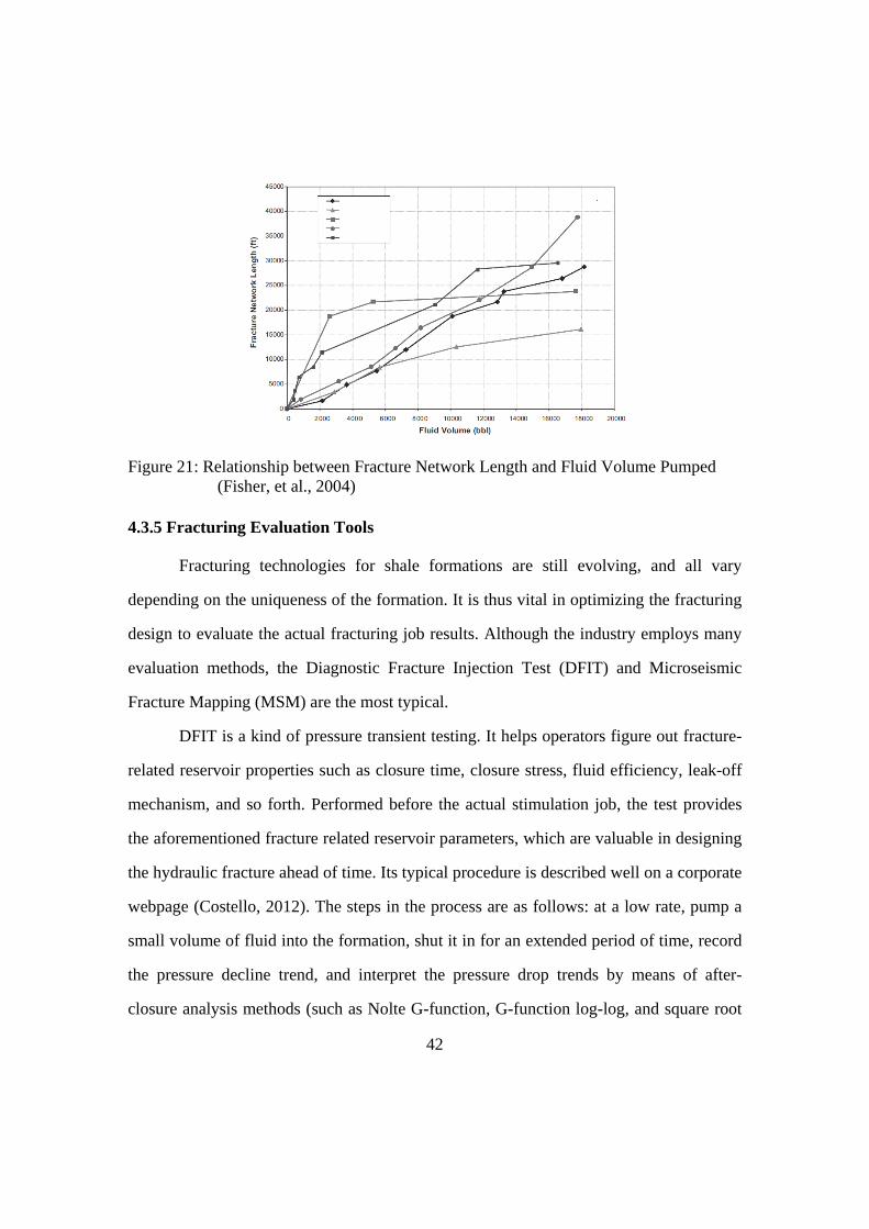
4.3.4 Treating Volume, Pressure and Injection Rate
There are many considerations concerning the stimulation job, for example, the
unique properties of the stimulated formations, frac fluid, well design, and so on. Another
formidable task, however, to ensure successful stimulations is deciding on treating fluid
volume, pressure, and injection rate. Treating fluid volume should be determined by
considering the positive relationship between the fluid volume and fracture network size
(shown in Figure 21). Surface treating pressure should be determined based on the frac
gradient specific to each formation, frictions at every point, casing rating, design safety
factor, etc. (Kundert & Mullen, 2009). Frac-fluid injection rates should have a fluid
velocity great enough to transport proppants without the proppants settling en route.
42
Figure 21: Relationship between Fracture Network Length and Fluid Volume Pumped (Fisher, et al., 2004)
4.3.5 Fracturing Evaluation Tools
Fracturing technologies for shale formations are still evolving, and all vary
depending on the uniqueness of the formation. It is thus vital in optimizing the fracturing
design to evaluate the actual fracturing job results. Although the industry employs many
evaluation methods, the Diagnostic Fracture Injection Test (DFIT) and Microseismic
Fracture Mapping (MSM) are the most typical.
DFIT is a kind of pressure transient testing. It helps operators figure out fracture-
related reservoir properties such as closure time, closure stress, fluid efficiency, leak-off
mechanism, and so forth. Performed before the actual stimulation job, the test provides
the aforementioned fracture related reservoir parameters, which are valuable in designing
the hydraulic fracture ahead of time. Its typical procedure is described well on a corporate
webpage (Costello, 2012). The steps in the process are as follows: at a low rate, pump a
small volume of fluid into the formation, shut it in for an extended period of time, record
the pressure decline trend, and interpret the pressure drop trends by means of after-
closure analysis methods (such as Nolte G-function, G-function log-log, and square root

43
of shut in time). A game changer, when it comes to hydraulic fracturing technologies, is
how one might refer to MSM. MSM has proved to be a useful tool providing a wide
range of parameters for understanding and optimizing hydraulic fracturing design. These
parameters include fracture geometry, complexity, stress azimuth, fault interactions, and
so on (Warpinski, 2009). Many researchers’ findings on the relationship between fracture
properties such as SRV and fracture complexity and gas production are attributable to
MSM technology. Despite its mighty utility, Cipolla (Cipolla, et al., 2010) considered it a
shortcoming that MSM requires separate monitoring wells. After all, Cipolla pointed out,
microseismic events cannot be sensed at the surface and a nearby offset wellbore should
be drilled (within 1000~3000ft of the treatment well; Figure 22, left). They argue this
disadvantage might be more serious outside the US where exploration infrastructures are
unestablished. At this point in time, the best solution seems to be a combination of
petrophysical log and MSM (Figure 22, Right) for evaluating and optimizing hydraulic
fracturing design.
Figure 22: Measurement of microseismic events (Left) (Cipolla, et al., 2010) Example of the results (Right) (Kundert & Mullen, 2009)

44
Chapter 5: Economic Challenges
A shale gas project is beset by many challenges affecting its economics. These
include predicting the future of natural gas prices and hedging against any unexpected,
drastic price drops, leasing an acreage with a minimum royalty, considering the
applicable tax regime including depreciation and depletion, and still others. This section,
however, sets aside those challenges, for they are general and have been covered
frequently in the past concerning conventional oil and gas projects. This section instead
concentrates solely on shale gas projects’ high initial well cost and their unique
production profile.
5.1 HIGH COST OF NEW TECHNOLOGIES
The two new technologies raised the ultimate production and made shale gas
plays economically viable. The down side is that they also spurred a drastic increase in
the initial development capital costs. Therefore, shale gas project developers must figure
out how to offset the high initial capital cost with the revenue growth from the
corresponding production increase.
As shown in Table 9, a horizontal well with a 4000ft lateral costs nearly triple a
vertical well. This high cost of horizontal drilling is understandable if we take into
account that horizontal wells go longer distances and consequently take longer to drill,
and require special, expensive equipment for directional drilling such as Rotary Steerable
Systems (RSS). In 2009, the rental fee for a horizontal drilling rig was as much as
US$ 22,100 per day (Proctor, 2010).

45
Table 9: Cost of vertical vs. horizontal wells (Schweitzer & Bilgesu, 2009)
Hydraulic fracturing technology is also high-priced due to its specialized
equipment and materials. Fluid storage tanks, proppant-transport equipment, blending
equipment, pumping equipment, and monitoring and control equipment could be
considered as a base fixed cost which is irrelevant to the number of fracturing stages or
frac half length (Distance that fractures propagate from the wellbore). On the other hand,
variable costs include such materials as fracturing water, additives, and proppants. From
Table 10, we can roughly predict the cost of a hydraulic fracturing job with 8 stages and
1000ft frac half length (as much as US$1,400,000). In addition, we should not overlook
water treatment and disposal costs; flowback water contains large amounts of total
dissolved solids (TDS). Figure 23 illustrates what other costs incur when it comes to a
horizontal well with hydraulic fracturing treatments.
Table 10: Cost of Hydraulic Fracturing (Schweitzer, 2009)
for average Marcellus shale wells

46
Figure 23: Average 2011 Fayetteville Shale Well Cost Estimate (SWN (SouthWest Energy), n.d.)
5.2 DETERMINATION OF ESTIMATED ULTIMATE RECOVERY (EUR)
The next challenge in the economic analysis of shale gas development projects is
how to determine total shale gas production over the entire project period. This notion is
typically expressed by the estimated ultimate recovery (EUR). Various methods can
determine EUR. These include material balance analysis, numerical simulation, decline
curve analysis (DCA), volumetric analysis, and analogy. DCA, however, is most
commonly used to forecast shale gas production because it is relatively easy and quick
(Baihly, et al., 2010a).

47
5.2.1 Decline Curve Analysis (DCA)
The basic concept of DCA, first introduced by Arps, is to extrapolate, by
equation, a production rate curve made from historical production data. From this the
entire production profile is constructed. The so-called Arps’ equation (Arps, 1945) is as
follows:
Q t1 /
where Q(t) is the gas production rate at time t, is the initial production rate, Di is the
decline rate in the first time period, and b is a parameter affecting the curvature of the
decline curve. In particular, the decline curve type is determined by the b value:
exponential (b = 0), harmonic (b = 1), and hyperbolic (b = other value). Shale gas
reservoirs have b values greater than 1, which, as shown in Figure 24, make curves
decline steeply in the first part and gently in the latter. These two distinct decline trends
in one production profile are attributed to the difference of their flow characteristics. The
initial steep decline is due to the boundary-dominated flow caused by hydraulic fractures
and the gentler decline in the latter part is due to the matrix-dominated flow caused by
matrix with very low permeability (Baihly, et al., 2010a).
Among the three parameters affecting EUR, b is the most controversial. The other
two parameters, Qi and Di, can be easily determined in the very beginning project stage;
it is not simple to calculate the b value from a very short period of historical production
data. Thus a sufficient production period is necessary to obtain a more accurate b value.
Furthermore, the regression results based on the limited historical production data can
vary with subjective interpreters. Figure 24 demonstrates, as an extreme case, how big a
difference in EUR a change of the b value makes. EUR 1.8 bcf with a b value of 0
increases more than 4 times to EUR 7.6 bcf with a b value of 2.

48
Figure 24: EUR difference with varying b values (Dean, 2008)
Berman (Berman, 2011) criticizes for several reasons EUR forecasting based on
this DCA method. Berman argues that a hyperbolic decline curve, which guarantees
longer well life, and larger EUR with a long tail could, as shown in Figure 25, be
interpreted with two-stage exponential decline. With the two-stage exponential decline
curve, EUR tumbled by more than half from 2.8 Bcf to 1.3 Bcf, and well life was
shortened by one fourth. Berman also argues that shale gas wells tend to show a
hyperbolic curve because of survivorship bias and re-stimulations. Only better
performing wells survive over time and influence the average production rate while poor

49
performing wells are abandoned and overlooked in the average production. Re-
stimulations could boost exponentially declining production and make the curve flatter.
Figure 25: Extrapolation of Barnett Shale Decline Curve with a same production history (Two Stage Exponential vs. Hyperbolic Decline) (Berman, 2011)
5.3 STRATEGIES
How to overcome the challenge of new technologies’ high cost is, in a sense,
simple. Eventually, the high cost cannot help but be offset by more production by means
of technological advancement. As this paper has already covered the technological

50
research efforts to produce more shale gas, the paper here addresses, using economic
analysis, how the relationship between cost and production can influence the profitability
of a shale gas project
5.3.1 Optimization of Well Design and Completion
A way to realize maximum production with minimum cost is to optimize the well
design and completion. Figure 26 illustrates what fracture length will produce the
maximum profit (Revenue minus cost). While the incremental revenue diminishes as the
fracture length increases, the cost rises faster. Hence, an optimal point can be found in the
fracture length (Holditch, et al., 1978). Shale gas developers should try to locate these
optimal points for not only fracture length but also for other elements of well design and
completion. These would include the number of fractures and lateral length of horizontal
wells. Schweitzer and Bilgesu (Schweitzer & Bilgesu, 2009) propose that a horizontal
well with nine fracs with 1000ft of half length and 4000ft of lateral leads to the highest
IRR.
Figure 26: Fracture Treatment Optimization Process (EPA, 2004)

51
5.3.2 Probabilistic Approach in the Resource Economic Evaluation
Such uncertainties as well cost and production parameters (b, Di, Qi) could of
course have a considerable impact on the economic feasibility of a project. Shale gas
developers, when evaluating the commercial viability of a shale gas well, should thus
take a probabilistic rather than a deterministic approach. Some researchers ( (Harding,
2008), (Gray, et al., 2007)) claim that the probabilistic or stochastic approach is more
suitable than the conventional, deterministic approach. Indeed, the latter merely reflects
the variability of inputs in the analysis by running sensitivity analysis. The economic
feasibility can consequently be estimated incorrectly due to the varying characteristics of
shale gas plays. Such characteristics include uncertainty of the area’s extent, geological
and petrophysical complexity, and high initial capital costs. These researchers argue that
trying to find proper statistical distributions for all uncertain inputs and obtaining a range
of outcomes can provide managers better insights when they must decide whether to
proceed or discontinue operations. Figure 27 shows how inputs and outputs are expressed
in the form of the statistical distribution.

52
Figure 27: Examples of Statistical Distributions of Inputs (up) and Outputs (down) (Harding, 2008)
5.3.3 Cost Reduction along a Learning Curve
As with any industry, costs associated with shale gas projects should drop as the
number of wells drilled rise. There is no reason to be frustrated by the high initial well
cost and the consequent negative NPV. As shown in Figure 28, the presentation material
by a consulting company (Wright & Company, Inc. , 2009) explains well the factors that,
regarding average EUR, contribute to forming an S-learning curve at each stage. The
initial stage curves gently upward as geological knowledge increases and the regulatory
process speeds up. The middle stage accelerates sharply as drilling and completion
techniques are optimized. In the last stage, the average EUR still increases though it
slows down as the economy of scale is realized and necessary infrastructures are in place.
Therefore, for a more accurate economic evaluation, developers and investors should take
into account the cost reduction along the learning curve, as shown in Figure 29.
Figure 28: Marcellus Shale Learning Curve (Wright & Company, Inc. , 2009)

53
Figure 29: Cost reduction over well count (Gray, et al., 2007)
5.3.4 Economic Analysis
Whether or not the high well cost and the decline curve with a shorter tail are
economically feasible can be verified through an elaborate economic analysis. A
simplified trial economic analysis was performed with a self-made Excel model for five
shale gas basins. This was done to show how the well cost and the decline curve
influence the economics of a shale gas well. In addition, the Excel add-on program, @
Risk, was utilized to run Monte Carlo simulation so that uncertainties with various
statistical distributions were reflected in the economic analysis.
5.3.4.1 Methodology
The cost and production profile, the most essential part of an economic analysis
for shale gas projects, was obtained from Baihly (Baihly, et al., 2010a). While well cost,
royalties, and operating cost were used as a base case without any adjustments, the
production profile was re-created with Excel by putting initial productions (IP), b values,
and Di values that the paper presents into the aforementioned decline curve formula.

54
However, Di values were adjusted to more closely match the EUR values that the paper
presents. Table 11 displays the figures from the paper. Figure 30 is the production profile
derived, using Excel, from Table 11. With this data, I performed two economic analyses
for only one well, as shown below. It is too complicated to perform an economic analysis
of hundreds of wells without making this a large scale of project. Moreover, there are
many other considerations (transportation cost, infrastructures, well spacing, well
development schedule, etc) that go beyond the research scope and purpose of this thesis.
Play Well cost
($MM)
Royalty
(%)
Operating Cost
($/Mscf)
b Di
(M.n)
EUR
(MMscf)
Haynesville 8 25 2.5 1.1852 0.0632 5,915
Eagle Ford 5.8 25 1.5 1.694 0.0826 3,793
Barnett 3 22 0.7 1.5933 0.0089 2,989
Fayetteville 2.8 17 1.1 0.6377 0.0325 1,390
Woodford 6.7 19 1.15 0.8436 0.0227 1,696
Table 11: Shale basin costs and decline curve parameters (Baihly, et al., 2010a)

55
Figure 30: Production profile for five basins
Economic Analysis for the optimization of fracture half length (Analysis I)
To demonstrate the optimization process, I examined how Net Present Value
(NPV) changes as the fracture half length increases. I also investigated at what fracture
length the NPV increase reversed. In addition, a tornado sensitivity chart was also drawn
for five uncertainties with 20% sensitivity. In particular, the b value is focused on to see
how incorrect matching (incorrect b value) can impact NPV. This analysis was performed
in a deterministic approach only for the Barnett shale basin
Statistical Analysis (Analysis II)
Using the data above, I calculated NPV and IRR of Free Cash Flow (FCF) over a
30-year period to investigate the economic viability of five shale gas basins. I divided
economic parameters into constants and uncertainties. I set as constants Weighted
Average Cost of Capital (WACC), inflation rate, tax, royalty, and the depreciation period.
I set as uncertainties, with their own statistical distributions, the initial production rate, b
value, natural gas wellhead price, Capex(Well cost), and Opex. Then, Monte Carlo
‐
200,000
400,000
600,000
800,000
1,000,000
1,200,000
1,400,000
1,600,000
1,800,000
2,000,000
0 5 10 15 20 25 30
Yearly production (mcf)
Year
Barnett Production (mcf)
Feyetteville Production (mcf)
Hanesville Production (mcf)
Woodford Production (mcf)
Eagle Ford Production (mcf)

56
simulation was performed with @Risk to obtain a range of outcomes (NPV and IRR with
chances)
5.3.4.2 Major Assumptions
The purpose of this economic analysis is not to evaluate a shale gas well in detail
but to demonstrate how to perform the economic analysis to cope with the
aforementioned economic challenges. Serious industrial economic analysis should be
performed by the help of professional reservoir simulation programs and economic
analysis tools and based on reliable distributions of uncertainties, which are made by
multi-disciplinary teams.
Analysis I
1. Hydraulic fracturing half length affects only the initial production rate (IP),
though in reality it influences b and Di values.
2. The initial production rate increases linearly with unit half length (250ft),
e.g., IP for 750ft of half length = IP for 250ft of half length x 3
3. Hydraulic fracturing cost increases exponentially with half length as shown in
Figure 4.
Analysis II
1. Means for the distributions of uncertainties are the values from Baihly’s paper
(Baihly, et al., 2010a).
2. Standard deviations for the distributions of uncertainties were picked arbitrarily,
which was inevitable because production and cost data are typically proprietary.
3. The distribution type of all uncertainties was set as lognormal according to
Harding (Harding, 2008)

57
4. Mean and standard deviation for only wellhead price were calculated based on
actual natural gas wellhead price history (EIA, n.d.)
5.3.4.3 Results
Analysis I
Figure 31: NPV vs. Fracture Half Length
As shown in Figure 31, 1000ft of fracture half-length led to the maximum NPV.
Figure 32: Tornado Sensitivity Chart for NPV of Barnett shale gas well
‐0.60
‐0.40
‐0.20
0.00
0.20
0.40
0.60
0.80
1.00
0 250 500 750 1000 1250 1500
NPV ($MM)
Fracture Half Length (ft)
Optimum point
0.41 0.61 0.81 1.01 1.21 1.41 1.61 1.81 2.01
Price
Initial production
b value
Well cost
Opex
NPV ($MM)
‐20 Pct +20 Pct
‐38% 38%

58
As expected, NPV was the most sensitive to the natural gas wellhead price; the
impact of operating cost was negligible. It is noticeable that, in terms of the influence on
NPV, the b value was compatible with the initial production and well cost.
Analysis II
A simulation for the Barnett shale basin resulted in the following two probability
distributions, shown in Figure 33. When NPV = 0, I could read the probability of failure
as 39.0%. And, I read P50 and P90 values of NPV and IRR from the distributions. I then
compiled the results into Table 12 by repeating the same simulation process.
Figure 33: NPV and IRR probability distribution of Barnett shale basin
-5 0 5 10 15 20 25 30
48.2% 10.3%
12.5% 45.0%
-50% 0% 50%
100%
150%
200%
250%
300%
350%
0.0
0.5
1.0
1.5
2.0
2.5
3.0
3.5
4.0
0.0%
12.5%
25.0%
37.5%
50.0%
62.5%
75.0%
87.5%
100.0%
IRR
IRR
Minimum -4.77%Maximum 317%Mean 20.2%Std Dev 22.8%Values 1000

59
Play NPV IRR
P of Failure (%)
P50 ($MM)
P90 ($MM)
P50 (%)
P90 (%)
Haynesville 77.5 -3.0 3.75 1.0 22.5.
Eagle Ford 74.2 -1.25 2 5.0 21.0
Barnett 39.0 0.5 5 12.5 45.0
Barnett Trial 65.0 0.5 10 12.5 80.0
Fayetteville 37.2 0.75 6.5 15.0 70.0
Woodford 79.1 -1.45 1.5 4.6 18.0
Table 12: Major Percentile Values of NPV and IRR
5.3.4.4 Findings and Implications
Analysis I
1. The optimization of fracture half length
Even though the resultant graph (Figure 31) shows the optimum point clearly, it is
presumed that the process to find an optimum well design and the resultant graph would
be even more complicated in a real project evaluation. There are many other well designs
and completion options such as horizontal lateral length, the amount of fracturing,
fracturing spacing, multilateral wells, a selection of fracture fluids, and so on.
2. Sensitivity Test
Just like other industrial sectors, the natural gas price was the most influential on the
economics of the Barnett shale gas project. The price, however, is a risk element beyond
operators’ control. Operators and investors can prepare for drastic price changes (and the
consequential loss) only with financial hedging strategies like swap or collar (cap or
floor) contracts. Other factors besides the Opex have a similar level of impact on NPV. It
is worth noting that a 20% change in the b value yields a 38% NPV difference. Unlike IP

60
and well cost, the b value can be determined after gathering quite a long production
history. This means a small mistake in calculating the b value might distort the economic
viability of a shale gas project. Therefore, examining closely whether the b value is
calculated based on a reliable production history is critical. Indeed, the b value may get
manipulated by operators set on attracting as many investors as possible.
Analysis II
The probability distributions in Figure 33 are unreliable. The distributions of
major uncertainties were made based on groundless assumptions where the standard
deviation and distribution type were set arbitrarily. What is important is that decision
makers are given more insightful analysis with the NPV or IRR distributions than only
the fixed numbers of NPV or IRR. For example, without the NPV distribution, the
decision makers could never know that there is a 39% chance of failure and a 10%
chance of profiting 6.5 million dollars in a Barnett shale gas project with only a fixed
NPV number (e.g., P50 NPV value of 0.5 million dollars). For decision makers of a risk-
seeking nature, a Barnett Trial boxed with a rectangular, which I made virtually as an
example, might be preferable to the original Barnett project (preferred perhaps by risk-
averse decision makers). After all, the statistical approach can reflect the decision
makers’ attitudes to risks and may lead to better decisions.
P50 NPV values can be considered reliable enough to judge the economic
feasibility of the project of a shale basin, as at least mean values of uncertainties were not
virtual but real. Based on P50 NPV values, only projects in Barnett and Fayetteville are
economically viable despite the lingering chance of failure if uncertainties move
negatively (e.g. unexpected drop in natural gas prices, increase in well costs, or
disappointing initial production). In contrast, the other projects, to be profitable, would
require uncertainties to move positively.

61
Chapter 6: Environmental Challenges
Environmental challenges surrounding hydraulic fracturing might be so serious as
to halt the project. It is not a matter of whether it is economic or not but a matter of
whether to go forward or not. While many environmental issues associated with shale gas
development are cited by environmentalists and media, the water-related issues are the
most controversial and have garnered the greatest attention. It’s no wonder that’s the case
considering that 98% of hydraulic fracturing fluid is water. Other environmental
problems such as air pollution, noise pollution, and induced earthquakes are not unique to
shale gas projects but apply to conventional oil and gas development projects. Therefore,
this section will concentrate on the environmental challenges concerning water.
6.1 WATER CONTAMINATION
6.1.1 Fracturing Fluids and Flowback Water
Two major reasons account for why water contamination is the most problematic
of shale gas development. One is that shale gas development requires a considerable
quantity of fracturing fluids that contain a variety of additives. The other is that part of
the fracturing fluid returns to the wellhead after its injection into the formation.

62
Figure 34: Volumetric Composition of a Fracture Fluid (GWPC, 2009)
Shale gas developers inevitably put various additives, as shown in Figure 34, in
the water to maximize the fracturing effects. The number and kind of the additives vary
according to the characteristics of the water and the target formation and the proprietary
know-how of service companies. Nevertheless, those considered compulsory are
proppant, friction reducer, acid, and surfactants. Primary additives, their roles, and their
compounds are presented in Table 5 of the previous chapter. While a report by GWPC
(GWPC, 2009), asserts that the chemical additives are safe as long as they are used in
small quantities and handled properly, service companies might still add hazardous
chemicals to maximize the effect of hydraulic fracturing. Hence, some US states
(Wyoming, Pennsylvania, Texas, and others) require service companies of hydraulic
fracturing to disclose the components of their additives.
The reason why the fracturing fluids with chemical additives cause environmental
concerns is that part of the injected fracturing fluids flows back to the surface. The flow
back rate (ratio of flow back water to originally injected fracturing fluids) could range
from 30% to as much as 70% (GWPC, 2009). The remaining fracturing fluids in the

63
formation might come out over an extended period with produced water. Further, the
flowback water may contain other dissolved natural constituents from the target
formation aside from the additives of fracturing fluid.
6.1.2 High Total Dissolved Solids (TDS)
Even if flow back occurs of fracturing fluids containing hazardous chemical
additives, there might still be no problem if the concentration of the additives is low
enough that they may be disposed of, untreated, in a nearby surface water body.
However, the TDS (Total Dissolved Solids) of the flow back water was reported to be
from 5000ppm to values greater than 400,000ppm (GWPC, 2009). Wastewater with TDS
greater than 200,000ppm cannot be processed and cleaned with normal water treatment
facilities like those used for general municipal purposes (Karbo, 2010). This means that
shale gas operators bear the additional cost of procuring a dedicated treatment facility,
transporting the wastewater to a suitable disposal site, or utilizing a UIC class II disposal
well.
6.1.3 Contamination of Groundwater and Surface Water
Fracturing fluids can come in contact with water used by humans through three
main avenues. The first is that fracturing fluids during the injection, or the flow back
water after the injection, might leak through the casing and invade groundwater near the
wellbore. The second is that the flow back water that returned to the surface or fracturing
fluids in storage or transit may, through accidental spills, contaminate nearby surface
water. The third way is that the injected fracturing fluids in the formation propagate
upward to groundwater level from the unit being fractured.
Various authors have rated as low, as long as proper safety measures are taken,
the chance that the first two cases might happen. Arthur (Arthur, et al., 2008) argues that

64
the chance of fracturing fluids’ leak-off through casing due to its corrosion is, based on a
study by API, less than that of general injection wells. The study, performed in the 1980s
when casing technologies and regulations were not as good as now, was performed for
water injection wells, which are operated at higher pressure and higher flow rates than
shale gas wells. Given this, the article presumes that the leak off probability of shale gas
wells must be lower than the range for the general water injection wells, 2 10 to
2 10 . Regarding the risk that fracturing fluids in storage and transport or flow back
water after a fracturing job may contaminate nearby surface water or soil, this can be
prevented by human effort. As for an overflow of an open pit containing flow back water
can be prevented by special equipment like enclosed steel tanks and by frequent
monitoring and testing (Zoback, et al., 2010)
Several studies ( (Arthur, et al., 2008), (Zoback, et al., 2010), (GWPC, 2009))
judge as slim the chance that injected fracturing fluids would propagate upward to the
level of groundwater. They offer two reasons. First, the target formation depth, as shown
in Figure 35, is far below the groundwater level. The target depth of fracturing jobs
typically ranges from 4,000ft to 12,000ft; groundwater level is usually less than 1,000ft.
Considering that the fracturing half length is 1,000ft at its longest, 3000ft separate the
two. Second, impermeable shale layers above the depth of fracturing preclude its
extensive upward movement. Nine layers of impermeable shale, for example, lay
between the target depth of Marcellus shale and the nearest groundwater (Arthur, et al.,
2008). A study of hydraulic fracturing environmental impacts in the Barnett, Haynesville,
and Marcellus plays found no evidence of groundwater contamination from the hydraulic
fracturing process (Groat & Grimshaw, 2012)

65
Figure 35: Target Shale Depth and Base of Groundwater (GWPC, 2009)
6.2 WATER AVAILABILITY
Another major challenge is securing sufficient water for drilling and for the
hydraulic fracturing of a shale gas well. The fracturing job of a horizontal shale gas well
consumes from 2 to 10 million gallons of water. The required amount varies with the
depth and permeability of the formation (ProChemTech Int. , 2009). As the consumption
might appear small compared to other demands, this challenge could be considered
trivial. The water use for electricity generation in Susquehanna River Basin is 150 million
gallons per day; the water use for hydraulic fracturing is merely 8.4 million gallons per
day (Gaudlip, 2008). However, this issue becomes serious in places like drought-prone
Texas or in Pennsylvania where surface water withdrawal is regulated. Moreover, shale
gas wells are not always close to water sources even in water-rich regions. Thus,

66
additional water transportation costs like trucking or pipelines might affect the economics
of the project.
6.3 PUBLIC CONCERN AND ENVIRONMENTAL REGULATIONS
A big challenge that lays ahead for many shale gas developers is The media and
environmental groups, with no proven evidence, try to attribute any accidental events in
the shale gas well sites to the risks associated with hydraulic fracturing. The media
covered the 2010 Clearfield blowout in the Marcellus shale basin as if hydraulic
fracturing were the direct cause of the accident. Of course, such a blowout could happen
in conventional oil and gas wells. On the other hand, major shale gas developers (e.g.,
Exxon’s TV commercials) take advantage of mass media to raise public awareness about
the safety of hydraulic fracturing.
Reflecting the aforementioned public concerns about hydraulic fracturing,
legislative activities and relevant research are now actively underway in the US. Sakmar
(Sakmar, 2010) explains the ongoing legislation activities surrounding the hydraulic
fracturing. Due to the insufficient content of a 2004 EPA report, public concern about
hydraulic fracturing escalated and was reflected in the 111th Congress. Two companion
bills, H.R. 2766 and S. 1215, the so called the Fracturing Responsibility and Awareness
of Chemical Act (the FRAC Act), was proposed. Congress also urged an in-depth study
by the EPA to decide whether hydraulic fracturing affects drinking water. The FRAC Act
prescribes that the injection of fluids for hydraulic fracturing should be regulated by the
underground injection provision of SDWA and that the chemical components of the
hydraulic fracturing fluids should be made public. The final report by the EPA
concerning the potential impact of hydraulic fracturing on drinking water is scheduled to
be released in 2014. Meanwhile, some states seem to have shelved any new drilling

67
permits as they await the federal law to be settled. New York State, one of several states
on the Marcellus Shale basin, passed in 2010 a moratorium banning additional drilling
that would accompany hydraulic fracturing jobs.
6.4 STRATEGIES
6.4.1 Proper Choice of Waste Water Disposal Options
There are largely three ways to dispose of the wastewater from a shale gas well:
underground injection, treatment and discharge, and recycling. GWPC (GWPC, 2009)
outlines the current status and problems of these three options.
Underground injection, which in the oil and gas industry has for decades been
considered the most common wastewater disposal method, could be the most suitable for
shale gas wastewater. This method injects shale gas wastewater thousands of feet
underground into saline aquifers through brine water disposal Class II injection wells
named by the EPA. The rock formation, however, should have sufficient pores to contain
the water and impermeable rock layers above to prevent the injected water from flowing
up to the groundwater. Moreover, Class II injection wells are strictly regulated by the
Underground Injection Control (UIC) program of the federal Safe Drinking Water Act
(SDWA). Accordingly, injection wells meeting the above conditions and still being close
to the field becomes problematic. If appropriate injection wells are not available nearby,
operators must consider transporting the wastewater to a remote injection well site or
other disposal options. Texas has tens of thousands of licensed Class II injection wells. In
contrast, the state of Pennsylvania with more political and geological restrictions has less
than a dozen (Zoback, et al., 2010)
The second option, treatment and discharge, is to treat the wastewater either at its
own treatment facility at the well site or at a distant, outside treatment facility and

68
discharge the treated water to nearby surface water bodies. In addition to the problem of
the wastewater transportation to a treatment facility, operators must consider the capacity
of the treatment facility. An existing commercial or municipal wastewater treatment
facility may lack the extra room to treat the shale gas wastewater. Moreover, TDS values
greater than 200,000ppm would exceed the processing power of the facility. If such is the
case, it would be necessary to consider constructing a dedicated local special treatment
facility.
The last option, recycling, is to re-use the treated water instead of discharging it.
The treatment facility for recycling should be located near the well site so that the treated
water can be re-used for the next fracturing jobs. In some cases, recycling, treatment for
re-use, seems more reasonable, especially considering that the water quality for discharge
to a surface body could be higher than the water quality for the hydraulic fracturing. The
recycling option should be adopted only after a careful review of a number of factors,
such as the concentration of the produced water, the processing power of the treatment
facility, minimum water quality for re-use, the construction cost of the treatment facility,
and so on.
The wise choice of a proper disposal option turns on a review of its necessary
costs and viability. If a shale gas well is close to a Class II injection well, transporting the
wastewater to the injection well would cost less than constructing a new treatment
facility, removing the consideration of the capacity and processing power of an existing
treatment facility. On the contrary, if a shale gas well is remote, far from either injection
wells or treatment facility, the best strategy may be to construct a dedicated treatment
facility and re-use the treated water for the subsequent fracturing.
Cost sharing with adjacent operators for capital-intensive strategies, such as the
construction of a pipeline to the injection wells or treatment facility and the construction

69
of a dedicated local injection well or treatment facility, could be an alternative. In the
case that project economics are affected unfavorably by constructing a treatment facility
or the laying of pipelines to transport the wastewater, then operators can reduce initial
construction cost by collaborating with other operators and realize an economy of scale.
6.4.2 Recycling Technologies
Recycling the flow back water and produced water is an effective solution for
both water contamination and water availability. This is especially true when other
options like underground injection or discharge of treated water are costly or illegal.
Recycled produced water can be re-used for future hydraulic fracturing and the decreased
volume of the remaining concentrated brine can contribute to reducing transportation
costs. In the case of the thermal distillation of the influent brine with 75,000mg/l TDS,
70% of the water is recovered and the final brine volume is reduced to nearly one-fifth
(Gaudlip, 2008).
Many wastewater treatment companies are still developing recycling
technologies based on those of conventional brine treatment. Companies have long
treated seawater, brackish groundwater, and produced water from conventional oil and
gas fields with such technologies as thermal distillation and reverse osmosis. Companies
are now developing recycling technologies for shale gas wastewater by applying the
conventional salt-water treatment technologies so as to fit the specific conditions of shale
gas wells. While the salinity of seawater is around 35,000ppm TDS, the TDS of flow
back water could be 50,000ppm and the TDS of produced water could reach as high as
250,000ppm (Barufet, et al., 2005). In the thermal distillation process, the heat exchanged
may be fouled by the components of flow back water (oils and greases, friction reducers,

70
and others), which are absent from conventionally produced water, seawater, and
groundwater (Gaudlip, 2008).
An operator must select a recycling technology best suited to the unique
characteristic of a shale gas well. Recycling technologies in the oil and gas industry vary
and each has its strengths and weaknesses. Ion Exchange is appropriate for low TDS
wastewater, reverse osmosis is preferred for waste water with TDS below 20,000 ppm,
and thermal distillation can treat water with TDS ranging from 40,000 to 100,000ppm
(Karbo, 2010). So, thermal distillation is the only option for high TDS wastewater
despite, as shown in Table 13, its high cost. Membrane-based systems like reverse
osmosis, which has good mobility (Gaudlip, 2008), can be a good alternative for well
fields where heavy truck traffic is a major problem.
Table 13: Performance of flow back recycling technologies (Harold, 2009)

71
Thermal Evaporation/Condensation
Some of the many recycling technologies cited as potential treatments of shale gas
waste water include reverse osmosis, ion exchange, and free thaw evaporation..
Currently, however, researchers have selected thermal evaporation/condensation
technology as the best way to handle the flowback and produced water of shale gas wells.
In particular, mechanical vapor recompression (MVR) is more prevalent over thermal
vapor recompression (TVR) in the shale gas industry (All consulting, 2011). Figure 36
shows, simply, how MVR works. MVR supplies heat to vapor through a compressor
rather than the boiler used by TVR. Based on information in Table 13, Harold (Harold,
2009) concludes, after comparing reverse osmosis and thermal evaporation/condensation
that the latter is currently best for recycling the flowback water of shale gas wells.
Despite its high unit cost, Harold justifies its selection on its efficiency (as high as 80%)
and its minimal and flexible energy inputs.
Figure 36: MVR Process (Fountain Quail)

72
6.4.3 Improvement in Fracturing Techniques
Water availability and water contamination pose serious enough threats to
jeopardize the existence of shale gas projects across the US. Hence, companies associated
with the fracturing process are endeavoring to improve the fracturing fluids and additives
themselves rather than struggling to procure water or worrying about wastewater
disposal. Service companies are trying to turn the performance oriented fracturing
additives into environmentally friendly components. Research firms, searching for an
innovative but hard-to-realize alternative, are venturing to change fracturing fluids from
water to other agents such as LPG or CO2.
6.4.3.1Environmentally friendly fracturing additives
Service companies, on their websites, are now boasting of their environmentally
friendly fracturing fluids. Halliburton proclaims that its CleanStim hydraulic fracturing
fluids are made with ingredients from the food industry. Halliburton assumes that
ingredients from the food industry, even if they spill by accident, are safe (Halliburton,
2011). BJ service eliminated from its water-based frac fluids benzene, ethylbenzene,
toluene, and xylene (BETX) components, all of which help increase the viscosity of the
fluids (BJ Services, 2011). Both companies argue that, based on their laboratory
experiments, they have sacrificed none of the fracturing performance with their
environmentally friendly fluids. A drilling chemistry company, Frac Tech, is reported to
be using orange citrus in place of some solvents and palm oil to replace a common
slicking agent (Lustgarten, 2009). Ultimately, however, the success of service companies’
efforts to replace or eliminate additives will come down to whether the fracturing
performance is maintained and the cost increase suppressed.

73
6.4.4.2 Alternative fracturing fluids
As water issues associated with hydraulic fracturing are being magnified as a
major controversy, service companies are trying to move away from water-based
fracturing fluids. As an alternative to water, LPG and CO2, despite some disadvantages,
show potential in actual shale gas wells.
Calgary-based GASFRAC Energy Services invented a technology that for a
fracturing fluid uses Liquefied Petroleum Gas (LPG). According to Smith (Smith, 2008),
LPG has various advantages over water. Due to its unique nature, the fracturing fluid’s
phase can alter, through a slight change in temperature and pressure, from liquid to gas.
In its liquid state, good for carrying proppants, it is pumped into the formation. It is
recovered in its gas state, good for escaping a formation, in particular, tight shale gas
formations. Consequently, the fluid recovery could be 100%, compare to 50% with
conventional fluids. The recovery time is reduced to as little as 48 hours while the
fracturing accomplishes two or three times a typical frac length. LPG fracturing has no
need to go through the so-called flaring process, a necessary procedure in conventional
fracturing. This saves half a million dollars worth of flared natural gas as well as reduces
the CO2 that would be naturally released by the process. Besides, as it is inert, LPG cause
no damage to the formation. LPG, however, has one critical disadvantage—it is highly
flammable. However, GASFRAC argues that such a shortcoming can be overcome by
equipment they developed that is fully enclosed and can be entirely operated remotely.
Also anticipated to replace water as fracturing fluids are CO2, N2, and methanol.
In particular, CO2-based fracturing systems, called Dry Frac, have shown their potential
in Canada and in U.S Department of Energy (DOE)-supported demonstration projects
(Gupta, 2009). CO2, like LPG, is pumped in as a liquid and recovered as a gas. It thus
avoids damaging the formation, which can frequently occur in conventional fracturing

74
and consequently impede gas production (Mazza, 2001). This is why the DOE tested
CO2-based fluids on the water sensitive Devonian Shale of eastern Kentucky.
Researchers have attempted to improve CO2 fluids’ shortcomings—its low viscosity and
high treatment costs of. One attempt mixed a foam of N2 into the CO2 liquid (Gupta,
2009). For CO2 to be used commercially, the process needs to overcome the challenges of
ice formation in the well stimulated by CO2 as well as the lack of infrastructure for
transporting CO2 and N2.
6.4.5 Establishment of Water Management Cooperative Organization
As meeting water challenges are usually beyond the practice of an individual
shale gas operator, it is desirable to form a cooperative organization for water
management issues including water sourcing and water contamination. Harold (Harold,
2009) offers a few solutions for handling these challenges. Operators could share a
wastewater recycling facility, they could push to amend regulations related to
groundwater withdrawals, and they could construct pipelines connecting well sites with
municipal or commercial wastewater treatment facilities. Such solutions can be realized
by the cooperation of operators in the same shale gas area. Barnett Shale Water
Conservation and Management Committee (BSWCMC), Appalachian Shale Water
Conservation and Management Committee (ASWCMC), and Marcellus Shale Coalition
(MSC) are current active shale gas developers. On its website, BSWCMC asserts its
mission as being “efficient and responsible water management, water conservation, and
environmental protection” and “estimating current and future water demands, conducting
proactive best management practices information transfer for industry, and identifying
technologies to provide effective solutions for water management” (BSWCMC, 2011).

75
Chapter 7: Challenges outside the US
Approximately 70% of the global shale gas reserves are located outside North
America (see Table 1 above). Nevertheless, the most substantive shale gas developments
are being made in North America. Martin (Martin, 2011) states that only nine wells were
drilled and fractured outside of North America. This suggests that North America has
some advantageous environments that facilitate developing shale gas resources.
Conversely, the absence of such advantageous conditions may present challenges for a
project developed outside of North America. For example, North America has well
established natural gas trunk lines and operators need not worry about the transportation
of produced gas to a consumption point. In contrast, shale gas developers in other regions
of the world like China should take into account a method of transporting the produced
gas to the end-users. Realizing such a method will lead to an increase in production costs.
7.1 LACK OF INFRASTRUCTURE
7.1.1 Service Companies, Equipment, and Information
One critical reason that shale gas development has been successful across the US
is the country’s well-developed oil and gas industry. Rigs that can support horizontal
drilling and hydraulic fracturing tasks can be rented at a relatively low price; oil and gas
service companies that can carry out those tasks efficiently are readily available in the
US. In other parts of the world, procuring shale gas development equipment and service
providers can be a formidable challenge.
Xiong (Xiong, 2006), a researcher working for Burlington Resources, which has
the rights to the CZ block in the Sichuan Basin, points out this challenge by citing the
case of shale gas development in China. Even though many international oil and gas

76
service companies have a presence in China, their scope of service is limited merely to
marketing or consulting without field operations. This appears to be due to the fact that
most Chinese national oil and gas companies have their own subsidiary service
companies and make them perform field operations with the assistance of the
international service companies. In regions beyond China, international service
companies with shale gas development know-how will also be under activity constraints
for the same reasons.
International oil and gas service companies do work in areas without such
constraints, yet they can still face such problems as importing the latest fracturing
equipment and obtaining relevant information. Xiong and Holditch (Xiong & Holditch,
2006) cite several key equipment items that are absent in China’s service market.
Equipment that is essential for efficient operation include precision continuous mixers
(PCM), snubbing unit, underbalanced drilling (UBD) pressure control, and multi-stage
compressors. Importing this equipment and adjusting them to the local situations requires
extra cost and leads to negative project economics.
A plethora of information related to shale gas development is considered a key
factor for America’s rapid shale gas growth. Government agencies like EIA or DOE
publish shale-gas-related research papers and statistical data regularly and information
sharing occurs through frequent technical meetings and workshops held across the US.
Most US states require operators to reveal a considerable amount of well information
(Martin, 2011). This easy information access contributes to project cost efficiency by
reducing technical or managerial errors in the initial stage or even in the middle of a
project. In contrast, project developers outside the US cannot expect this easy information
access. In some countries in Africa, even basic geological subsurface data might be
missing. Or, despite there being basic field data collected by local governmental

77
agencies, it might be nearly impossible to gain access to the data through a bureaucracy
like that of China’s. Xiong and Holditch (Xiong & Holditch, 2006) complain of this
bureaucracy and the lack of information sharing in China. After all, such a lack of
information flattens the project learning curve making it take longer for a project to reach
a breakeven point.
7.1.2 Transportation of produced gas
America’s well-established natural gas pipeline network, shown in Figure 37,
helps account for the country’s recent shale gas boom. By simply connecting a shale gas
well to the nearest pipeline, shale gas produced anywhere in the US can be transported
any place in the US. Shale gas developers in other regions are left to figure out ways to
transport the produced gas. In China, for example, shale gas produced in the Tarim basin,
as can be seen in Figure 38, needs a pipeline to connect with where natural gas demands
are high—the east of China. If domestic demand for natural gas is insufficient to
consume the produced shale gas, producers should take into account an LNG facility or
international pipeline system. As these options require a huge investment, they could,
without government support, doom the economics of shale gas projects.
Figure 37: US Natural Gas Pipeline Network, 2009 (EIA, 2009)

78
Figure 38: China Basins (Xiong & Holditch, 2006)
7. 2 UNCLEAR OR UNFAVORABLE POLICIES AND REGULATIONS
Today, America’s regulatory environment regarding shale gas development is
turning unfavorable. The public’s perception is that hydraulic fracturing negatively
impacts the environment. Yet they were the favorable governmental policies that
contributed to its rapid emergence in the US. Deloitte (Deloitte, 2011) asserts that a
major reason shale gas took off quickly in the US was the country’s easy land access. US
private landowners can hold not only surface rights but also mineral rights, so with
financial incentives like certain royalty rates they can be persuaded to lease these rights.
Martin (Martin, 2011) identifies another factor in America’s shale gas development as the
government’s tax credit in the 1980s through 1990s. The Alternative Fuel Production
Credit, under Article 29 of the Internal Revenue Code introduced in the 80s, provided an
income tax credit as much as $3 per BOE for hydrocarbon production from
unconventional natural resources like oil shale, tar sands, biomass, coal seams, and so on.

79
In contrast, most regions of the world have different regulatory settings for shale
gas development. In Europe, for example, surface rights are owned by individuals, while
the government retains possession of mineral rights. So, landowners who will be
compensated for only surface right are less attracted by offers from shale gas developers
and consequently cooperate less actively in the developers’ land acquisition. In China, on
the other hand, land acquisition might be easier than in America. There the government,
which has a strong will to develop its shale gas resources, hold exclusive rights to both
surface and mineral rights (Deloitte, 2011).
Shale gas developers could also be challenged by policy uncertainty associated
with shale gas development. Aside from the US, countries have only recently begun to
identify their shale gas potential. Thus, they have yet to establish policies or regulations
specific to shale gas or unconventional natural resources. The policies they establish
could be positive or negative. Governments could try to offset high costs due to the lack
of infrastructure by handing out tax benefits. On the other hand, they could establish
burdensome regulations to curb the destruction of the environment (like has been done in
New York). It all depends on the government’s viewpoint about its energy urgency and
the public’s perception of the environment. China, with its rapidly growing economy, is
struggling to secure sustainable energy sources. It then is more likely to adopt pro-shale
gas development policies. Europe might witness a collision between environmentalists
and supporters of shale gas development, which could alleviate Europe’s heavy
dependence on gas from Russia.

80
7.3 STRATEGIES
7.3.1 Targeting Countries with Urgent Needs or Favorable Conditions
To overcome the problem of the lack of infrastructures, developers should target
countries with existing infrastructures or with the high possibility of infrastructures being
quickly established. Shale gas, in composition, is the same as natural gas produced from
conventional sandstone or limestone formations. Hence, all existing natural gas facilities
whether for E&P or for exporting or importing, could be utilized for shale gas. In this
sense, good candidates for shale gas development might be some countries located in the
Middle East and North Africa, countries that are now producing conventional natural gas
and, at the same time, have considerable shale gas reserves. On the other hand, there are
some countries with substantial shale gas reserves such as China and Poland, which have
urgent political or economic needs to exploit the shale gas but lack sufficient
infrastructures to produce or transport it.
Martin (Martin, 2011), in evaluating the potential of shale gas developments in
the Middle East and North Africa, pays special attention to North African countries like
Algeria and Tunisia. Unlike the Middle Eastern gas producers who have to use LNG or to
construct additional long distance pipelines to export produced gas, North African
countries, as shown in Figure 39, have well-established export pipelines and LNG export
terminals. In addition, Europe’s natural gas network grid is connected to the North
African gas export pipeline system. And of course Europe, wanting to shed their
excessive dependence on Russian pipeline gas, has a motivation to import natural gas
from other sources. Moreover, as current natural gas exporters, countries like Algeria and
Egypt possess considerable natural gas production infrastructures.

81
Figure 39: North African Gas Export Infrastructure. Major pipelines in red lines and LNG export terminals as blue dots (Martin, 2011)
A good strategy to overcome the lack of infrastructures outside the US could be
this targeting of countries in urgent need of natural gas and of governments thought to be
accommodating in expanding shale gas infrastructures. Some International Oil
Companies (IOC) seem to have already identified (Table 14) a few of such countries—
China, Poland, Argentina, and others.
Poland depends on Russian natural gas for 43% of its natural gas consumption
(Gelb, 2007). Its energy security can be easily jeopardized by Russia cutting off its
supply or abruptly raising its prices. Russia might do this, as indeed it did in 2009 with
the Ukraine, as part of a dispute with an intermediate country. Being vulnerable to such
actions, Poland is largely cooperative towards exploration and development of shale gas
resources (Jones, et al., 2011).

82
Table 14: IOCs in Poland and China (Deloitte, 2011)
From both economic and environmental perspectives, China also feels an urgent
need to develop its shale gas resources. In 2009, China for the first time became a net gas
importer; its natural gas demand forecast for 2020 is three times its current level
(Deloitte, 2011). Thus the Chinese government should either build more importing
pipelines or LNG terminals or seek for domestic unconventional resources like shale gas
or tight gas. In addition, China cannot cope with the era of greenhouse gas reduction
represented by Kyoto protocol with its current energy mix in which coal accounts for
70% of the total. China’s recent series of events shown in Table 15 make shale gas
developers confident about the positive and active support from the Chinese government.
Such support is necessary to overcome the lack of infrastructures and regulatory issues
inevitable in the initial stage of shale gas development.
Country IOC Details
Poland ConocoPhillips In early 2010, a JV of ConocoPhillips and Lane Energy started drilling in the Baltic Basin in Northern Poland
Poland Chevron In February 2010, Chevron was granted five year exploration rights for four shale concessions: Zwierzyniec, Kransnik, Fampol and Grabowiec
China ExxonMobil In talks to jointly explore and develop Ordos basin in Northern China
China BP In talks to jointly explore and develop shale gas resource opportunitiesin the 42 shale gas blocks Sinopec already owns
China Chevron In talks to sign an agreement to jointly explore and develop shale gas in southwestern China, near the area BP is exploring
China Shell Evaluating shale gas assets in the Sichuan basin. Signed a 30 year contract to jointly appraise and potentially develop tight gas in the Jinqiu block of central Sichuan province

83
Table 15: Chinese government’s recent events for shale gas (Wang, et al., 2011)
7.3.2 Cooperation with Local Petroleum Companies and Government
As Martin research paper (Martin, 2011) points out, the lack of infrastructures for
shale gas development is a chicken-and-eggs problem. Service companies are reluctant to
invest considerable funds in countries where shale-gas-related activity is low. Yet the
activity level remains stagnant due to a lack of service companies in the country. Such a
country’s government can break this vicious circle by providing fiscal benefits like
America’s Alternative Fuel Production Credit. They can offer a tax exemption for
equipment imported for shale gas development or for the construction of exporting long
distance pipelines or LNG plants. Once the low development cost is realized, the
governmental beneficial policies can, as has been done in the case of the US, be removed.

84
What matters most for successful initial entry into the shale gas development
market of a country is to win as many benefits as possible by seeing to the host countries’
most urgent needs. In other words, international oil companies need to explain to the host
government the initial difficulties of shale gas development so as to procure appropriate
incentives to offset the high initial development cost. As in the case of the solutions
Martin offers to vitalize service companies in North Africa, oil companies should direct
their persuading of host governments at countries like Algeria, Egypt, and Libya. If goods
and services for shale gas development could move freely across the borders of adjacent
North African countries, the substantial investment from service companies could be
rewarded by the principle of economy of scale. The overall well cost would drop
accordingly (Martin, 2011).
Government aid is essential for successful shale gas development. IOCs should
thus consider strategic partnerships with local oil and gas companies or local service
companies. By and large, local oil companies not only have better connections with the
host government but also might have feasibility-study-levels of information on the
development area. Partnering with local companies could be mandatory in some
countries. Such is the case in China, where in the 2011 licensing round of its six shale gas
plays, the government permitted only joint bidding with domestic oil companies. Other
examples include Statoil’s JVs with Talisman and Chesapeake to develop Europe shale
basins, and PetroChina’s 2010 partnership with Encana and a joint venture of Weir Group
and Shengli Oilfield Highland Petroleum Equipment Company to develop Chinese shale
basins (Deloitte, 2011). As shown in Table 16, some IOCs seem to yield even their
homeland shale gas resources to strengthen mutual partnership for shale gas development
in China.

85
Table 16: Chinese Companies’ investment in the North America (Wang, et al., 2011)

86
Chapter 8: Conclusion
By investigating five categories of challenges for shale gas projects, I conclude
that shale gas project developers should examine and analyze all the challenges
thoroughly by making an overall checklist like that found in Table 17. Indeed, the
economics of most modern shale gas development projects are in a marginal state and if
even a small challenge is improperly addressed these projects’ profitability will be a net
minus. They should also check whether strategies are feasible or even available.
Strategies to the challenges have not been established systematically, are still under
research, or belong to only limited highly-experienced service companies.

87
Category Challenges Strategies
Identification
a. Different mechanism of shale formations
- Complex structure, adsorbed gas, natural
fractures
a. Different identification index
- TOC, stress, brittleness, TM, etc
b. Evaluation Tools (XRD, SEM, etc)
Technical
a. Ultralow permeability, Heterogeneity
b. Well design
- Well placement, lateral length
c. Drilling challenges
- Curve and lateral section
d. Hydraulic fracturing design
- Optimization of fractures
- Fracturing Fluids
- Treating volume, pressure, injection rate
a. Appraisal wells
b. Accurate reservoir characterization
c. Improved drilling techniques
- Rotary Steerable System (RSS)
- Logging While Drilling(LWD)
d. Fracturing Evaluation Tools
- Diagnostic Fracture Injection Test
(DFIT)
- Microseismic Mapping (MSM)
Economical
a. High cost of new technologies
- Horizontal drilling
- Hydraulic fracturing
b. Estimation of ultimate recovery
a. Optimization of well design and
completion in economical perspective
b. Cost reduction along learning curve
c. Probabilistic approach
Environmental
a. Water contamination
- Fracturing fluids and flowback water
b. Water Availability
c. Public concern and regulations
a. Proper water disposal
- Underground injection, treatment
and discharge, etc.
b. Recycling technologies
- Reverse Osmosis/Thermal
distillation
c. Improvement of fracking itself
d. Cooperative Organization
International a. Lack of Infrastructures
b. Unclear policies and regulations
a. Targeting prospective countries
b. Cooperation with local entities
Table 17: Exemplary Checklist for Shale Gas Development
Once balanced and comprehensive checkups on the challenges and strategies are
completed, the developers should select challenges they need to concentrate on more.
After all, every shale play has its own characteristics, and some challenges in a shale
project need special care and strategies. For the same reasons, it would be risky to take on

88
shale gas development thinking projects will follow the pattern of successful shale
projects like those in the Barnett Basin. For example, developers must deal seriously with
such challenges as water disposal in densely populated areas and the strictly regulated
Marcellus Basin, water availability in the Barnett Basin where frequent droughts occur,
as well as proppant embedment and fines generation in the Haynesville Basin which has
soft and friable shale.
In countries sensitive to environmental issues (the US and the EU), companies
must pay more heed to the environmental challenges than to others. Such challenges are
existential to a shale gas project; others, such as technical or economical challenges, are
just a matter of efficiency. Projected profits might suffer to a certain extent due to a
failure in the fracturing planning. On the other hand, a shale gas business itself might go
to nothing if the project developer fails to observe closely the trends of policies or studies
regarding environmental impacts of shale gas developments. These were the cases of
France and New York, both of whom recently banned the drilling for shale gas resources.
On top of the comprehensive checkup and intensive care about challenges specific
to a shale gas project, shale gas developers should keep themselves up to date with shale–
gas-related circumstances including rapid pace of shale gas technology advancement.
Conventional oil and gas projects operate on technologies and circumstances that are
stabilized to some extent. In contrast, shale gas developments are in a transitional period
and challenges, once difficult to cope with, might be addressed with adequate strategies.
For example, the challenges of understanding how hydraulic fractures propagated and
designing optimal fracture systems were lightened by the advent of microseismic
monitoring technology. Also, what once was a straightforward path may soon become a
regulatory thicket. For example, favorable stimulus policies for unconventional energy

89
sources like US tax credits turned into unfavorable regulatory policies, evidenced by the
moratorium of New York State on hydraulic fracturing.

90
References
Abou-Sayed, I. S. et al., 2011. HaynesVille shale Development Program - From Vertical to Horizontal. SPE 144425.
All consulting, 2011. Water Treatment Technology Fact Sheet. [Online] Available at: http://www.all-llc.com/publicdownloads/ThermalDisillationFactSheet.pdf [Accessed 24 January 2012].
Arps, J. J., 1945. Analysis of Decline Curves. Volume 160.
Arthur, J. D., Bohm, B. & Layne, M., 2008. Hydraulic Fracturing Considerations for Natural Gas Wells of the Marcellus Shale, s.l.: All consulting.
Azizov, A. et al., 2012. Optimized Steerable Motor Design Overcomes Drilling Challenges in the Fayetteville Shale Unconventional Play. SPE 151135.
Baihly, J., Altman, R., Malpani, R. & Luo, F., 2010a. Shale Gas Production Decline Trend Comparison Over Time and Basins. SPE 135555.
Baihly, J. D. et al., 2010b. Unlocking the Shale Mystery : How Lateral Measurements and Well Placement Impact Completions and Resultant Production. SPE 138427.
Bammidi, V., Balch, R. & Engler, T., 2011. Ranking the Resource Potential of the Woodford Shale in New Mexico. SPE 144576.
Barufet, M., Burnett, D. & Mareth, B., 2005. Modeling and Operation of Oil Removal and Desalting Oilfield Brines with Modular Units. SPE 95647.
Bell, C. & Brannon, H., 2011. Redesigning Fracturing Fluids for Improving Reliability and Well Performance in Horizontal Tight Gas Shale Applications. SPE 140107.
Berman, A. E., 2011. U.S. Shale Gas : Less Abundance, Higher Cost. [Online] Available at: http://www.theoildrum.com/node/8212 [Accessed 8 January 2012].
BJ Services, 2011. Environmentally Friendly Fracturing Fluids. [Online] Available at: http://www.bjservices.com/website/index.nsf/WebPages/Shale-Papers-Expandable-Section/$FILE/Environmentally%20Friendly%20 Fracturing%20Fluids%20Sales%20Bulletin%20rev%20082508.pdf [Accessed 24 January 2012].
Brooks, D., 2011. Shale Gas Revolution. New York Times, 3 November.
BSWCMC, 2011. Mission and Purposes of BSWCMC. [Online] Available at: http://www.barnettshalewater.org/mission-purpose.html [Accessed 27 January 2012].
Bustin, M., 2006. Geology report: where are the high-potential regions expected to be in Canada and the U.S.? Capturing opportunities in Canadian shale gas. Calgary, s.n.

91
Chaveste, A., Hall, M., Verm, R. & Geiser, J., 2011. Estimation of Fracture Density and Orientation through Azimuthal Processing and Interpretation of Seismic Data. SPE 148866.
Chelini, V. et al., 2010. Gas Shale Reservoir Characterization : North Africa Case. SPE 134292.
Chong, K. K. et al., 2010. A completion Guide Book to shale-Play Development: A Review of Successful Approach towards Shale-Play Stimulation in the last Two Decades. SPE 133874.
Cipolla, C., Lolon, E., Erdle, J. & Rubin, B., 2009. Reservoir Modeling in Shale Gas Reservoirs. SPE 125530.
Cipolla, C., Mack, M. & Maxwell, S., 2010. Reducing Exploration and Appraisal Risk in Low-Permeability Reservoirs Using Microseismic Fracturing Mapping. SPE 137437.
Cipolla, C. et al., 2011. New Algorithms and Integrated Workflow for Tight Gas and Shale Completions. SPE 146872.
Costello, C., 2012. Pre-frac Injection Fall-off Tests (DFIT) in Ultra Low Permeability Formations. [Online] Available at: http://www.spidr.com/oil-and-gas/Pre-frac-Injection-Fall-off-Tests-DFIT-in-Ultra-Low-Permeability-Formations/subpage128.html [Accessed 13 March 2012].
Crain, E. R., 2012. Special Cases – Gas Shales. [Online] Available at: http://www.spec2000.net/17-specshgas.htm#b4 [Accessed 10 March 2012].
Cramer, D., 2008. Stimulating unconventional reservoirs: lessons learned, successful practices, areas for improvement. SPE 114172.
Dean, L., 2008. Reservoir Engineering For Geologists” Part 4 – Production Decline Analysis. [Online] Available at: http://www.fekete.com/resources/papers/reservoir_engineering_geologists4_paper.pdf [Accessed 8 January 2012].
Deloitte, 2011. Revolution or Evolution. [Online] Available at: http://www.deloitte.com/assets/Dcom-UnitedStates/Local%20Assets/Documents/us_consulting_RevolutionorEvolution_Oilfield_Technology052511.pdf [Accessed 27 January 2012].
EIA, 2009. US natural gas pipeline network. [Online] Available at: http://www.eia.gov/pub/oil_gas/natural_gas/analysis_publications/ngpipeline/ngpipelines_map.html [Accessed 14 March 2012].
EIA, 2011a. Review of Emerging Resources : US Shale Gas ans Shale Oil Plays, s.l.: s.n.
EIA, 2011b. Technology drives natural gas production growth from shale gas formations.

92
EIA, 2011c. World Shale Gas Resources: An initial Assessment of 14 regions outside the United States, s.l.: s.n.
EIA, 2012a. Annual Energy Outlook 2012 Early Release Overview, s.l.: s.n.
EIA, n.d. U.S. Natural Gas Wellhead Price. [Online] Available at: http://www.eia.gov/dnav/ng/hist/n9190us3m.htm [Accessed 8 January 2012b].
EPA, 2004. Evaluation of Impacts to Underground Sources of Drinking Water by Hydraulic Fracturing of Coalbed Methane Reservoirs; Appendix A Hydraulic Fracturing White Paper.
Fekete Association Inc. , 2010. CBM Concepts. [Online] Available at: http://www.fekete.com/software/cbm/media/webhelp/c-te-concepts.htm [Accessed 26 Febrary 2012].
Fisher, M. et al., 2004. Optimizing Horizontal Completion Techniques in the Barnett Shale using Microseimic Fracture Mapping. SPE 90051.
Gaudlip, A. L., 2008. Marcellus Shale Water Management Challenges in Pennsylvania. s.l., s.n.
Gault, B. & Stotts, G., 2007. Improve Shale Gas Production Forcasts. [Online] Available at: http://www.epmag.com/EP-Magazine/archive/Improve-shale-gas-production-forecasts_306 [Accessed 26 Febrary 2012].
Gelb, B. A., 2007. Russian Natural Gas : Regional Dependence, s.l.: CRS Report for Congress.
Gray, W. M., Hoefer, T., Chiappe, A. & Koosh, V., 2007. A Probabilistic Approach to Shale Gas Economics. SPE 108053.
Grieser, B. & Bray, J., 2007a. Identification of Production Potential in Unconventional Reservoirs. SPE 106623.
Grieser, B. et al., 2007b. Surface Reactive Fluid's Effect on Shale. SPE 106815.
Groat, C. G. & Grimshaw, T. W., 2012. Fact-based Regulation for Environmental Protection in Shale Gas Development
Gupta, D., 2009. Unconventional Fracturing Fluids for Tight Gas Reservoirs. SPE 119424.
GWPC, (. W. P. C., 2009. Modern Shale Gas Development in the United States: a Primer, s.l.: s.n.
GWPC, 2009. Modern Shale Gas Development in the United States: a Primer, s.l.: GWPC (Ground Water Protection Council).
Halliburton, 2011. Clean Steam Hydraulic fracturing Fluid System.[Online] Available at: http://www.halliburton.com/ps/default.aspx?pageid=4184&navid=93&AdType=JPTCSTC [Accessed 24 January 2012].

93
Harding, N. R., 2008. Application of Stochastic Prospect Analysis for Shale Gas Reservoirs. SPE 114855.
Harold, J., 2009. Strategies to Reduce Terminal Water Consumption of Hydraulic Fracture Stimulation in the Barnett Shale, s.l.: UT at Austin.
Haskett, W. J. & Brown, P., 2005. Evaluation of Unconventional Resource Plays. SPE 96879.
Holditch, S., Jennings, J., Neuse, S. & Wyman, R., 1978. The Optimization of Well Spacing and Fracture Length in Low Permeability Gas Reservoirs. SPE 7496.
Hopkins, C., 1997. The Importance of In-situ Stress Profiles in Hydraulic Fracturing Applications. JPT.
Jones, F., Zimmerman, M. & Heinz, W., 2011. Managing Environmental Risks from Shale Gas Exploration – Applying Lessons Learned in the US to New Ventures in Poland. SPE 140864.
Karbo, D. M., 2010. Natural Gas Plays in the Marcellus Shale: Challenges and Potentials. Environmental Science & Technology, Volume 44.
Kundert, D. & Mullen, M., 2009. Proper Evaluation of Shale Gas Reservoirs Leads to a More Effective Hydraulic-Fracture Stimulation. SPE 123586.
LeCompte, B. & Hursan, G., 2010. Quantifying Source Rock Maturity From Logs : How to get more than TOC from delta log R. SPE 133128.
Lewis, R., 2004. New Evaluation Techniques for Gas Shale Reservoirs. s.l., s.n.
Lustgarten, A., 2009. Underused drilling practices could avoid pollution. [Online] Available at: http://www.propublica.org/feature/underused-drilling-practices-could-avoid-pollution-1214 [Accessed 24 January 2012].
Martin, A. N., 2011. The Potential Pitfalls of Using North American Tight and Shale Gas Development Techniques in the North African and Middle Eastern Enviornments, s.l.: s.n.
Mazza, R. L., 2001. Liquid-Free CO2/Sand Stimulations: An Overlooked Technology – Production Update. SPE 72383.
Mcfarland, G., 2010a. Going Long in the Oil Patch : Super Extended Lateral Completions. [Online] available at: http://www.oilandgasevaluationreport.com/2010/02/articles/horizontal-drilling-technology/going-long-in-the-oil-patch-super-extended-lateral-completions/ [Accessed 9 March 2012].
Mcfarland, G., 2010b. Petroleum Geochemistry and Shale Plays. [Online] Available at: http://www.oilandgasevaluationreport.com/tags/vitrinite-reflectance/ [Accessed 26 Febrary 2012].

94
Miller, R. S., 2010. Critical Elements of Gas Shale Evaluation; Core Laboratories. San Antonio, Texas, s.n.
Morrill, J. & Miskimins, J., 2012. Optimizing Hydraulic Fracture Spacing in Unconventional Shales. SPE 152595.
Passey, Q. R. et al., 1990. A Practical Model for Organic Richness from Porosity and Resistivity Logs. The American Association of Petroleum Geologists Bulletin.
Pemper, R. et al., 2009. The Direct Measurement of Carbon in Wells Containing Oil and Naturla Gas Using a Pulsed Neutron Minerology Tool. SPE 124234.
Pickering Engery Partners, 2005. The Barnett shale : Visitors Guide to the Hottest Gas Play in the US, s.l.: s.n.
Pope, C. et al., 2010. Improving Stimulation Effectiveness - Field Results in the Hayesville Shale. SPE 134165.
ProChemTech Int. , 2009. Innovations in water management. [Online] Available at: http://prochemtech.com/Literature/TAB/TAB_Marcellus_Hydrofracture_Disposal_0509.pdf [Accessed 15 January 2012].
Proctor, C., 2010. Rigs: Demand, cost up as supply falters. [Online] Available at: http://www.bizjournals.com/denver/print-edition/2010/12/10/rigs-demand-cost-up-as-supply-falters.html?page=3 [Accessed 7 January 2012].
Rickman, R. et al., 2008. A Practical Use of Shale Petrophysics for Stimulation Design Optimization: All Shale Plays Are Not Clones of the Barnett Shale. SPE 115258.
Rokosh, C. et al., 2009. What is Shale Gas? An Introduction to Shale-Gas Geology in Alberta, s.l.: s.n.
Sakmar, S. L., 2010. The Future of Unconventional Gas: Legal, Policy and Environmental Challenges to the Development of North American Shale Gas. Calgary, s.n.
Saldungaray, P. & Palisch, T. T., 2012. Hydraulic Fracture Optimization in Unconventional Reservoirs. SPE 151128.
Schweitzer, R. & Bilgesu, H., 2009. The Role of Economics on Well and Fracture Design Completions of Marcellus Shale wells. SPE 125975.
Scotland, M., 2011. Opportunity, Risks and Direction of the Shale Gas Market. [Online] Available at: http://naturalgasforamerica.com/opportunity-risks-direction-shale-gas-market.htm [Accessed 21 March 2012].
Shah, S. N., Vincent, M., Rodriquez, R. & Palisch, T., 2010. Fracture Orientation and Proppant Selection for Optimizing Production in Horizontal Wells. SPE 128612.
Smith, M., 2008. Frac Forward: Startup cracks propane fracture puzzle provides ‘Green’ solution. New Tech Mag..

95
Sorrell, M. e. a., 2011. Haynesville Shale Development Program – From Vertical to Horizontal. SPE 144425.
Sugiura, J. & Jones, S., 2010. Rotary Steerable System Enhances Dirlling Performance On Horizontal Shale Wells. SPE 131357.
SWN (SouthWest Energy), n.d. Investor Presentation. [Online] Available at: http://www.swn.com/Pages/default.aspx [Accessed 7 January 2012].
The Economist, 2011. Fracking here, fracking there. The Economist, 26 November.
Walsh, B., 2011. Could Shale Gas Power the World?. Time Magazine, 31 March.
Wang, X., Jiang, R. & Wang, S., 2011. The Shale Gas Potential of China. SPE 142304.
Warpinski, N. R., 2009. Intetrating Microseimic Monitoring with Well Completions, ReservoirBehavior, and Rock Mechnics. SPE 125239.
Wright & Company, Inc. , 2009. The Marcellus Shale Learning Curve : The results and Challenges. [Online] Available at: http://www.wrightandcompany.com/FINAL%20Wright%20&%20Company%20DUG%20East%20Presentation.pdf [Accessed 9 January 2012].
Xiong, H. e. a., 2006. Will the Blossom of Unconventional Natural Gas Development in North America Be Repeated in China. SPE 103775.
Xiong, H. & Holditch, S., 2006. Will the Blossom of Unconventional Natural Gas Development in North America Be Repeated in China. SPE 103775.
Zoback, M., Kitasei, S. & Copithorne, B., 2010. Addressing the Environmental Risks from Shale Gas Development, s.l.: Worldwatch Institute.