Copyright © 2001, 2003, Andrew W. Moore Entropy and Information Gain Andrew W. Moore Professor School of Computer Science Carnegie Mellon University awm

Copyright © 2001, 2003, Andrew W. Moore

Entropy and Information Gain

Andrew W. MooreProfessor

School of Computer ScienceCarnegie Mellon University

www.cs.cmu.edu/[email protected]

412-268-7599

Note to other teachers and users of these slides. Andrew would be delighted if you found this source material useful in giving your own lectures. Feel free to use these slides verbatim, or to modify them to fit your own needs. PowerPoint originals are available. If you make use of a significant portion of these slides in your own lecture, please include this message, or the following link to the source repository of Andrew’s tutorials: http://www.cs.cmu.edu/~awm/tutorials . Comments and corrections gratefully received.

http://www.cs.cmu.edu/~awm/tutorials

Copyright © 2001, 2003, Andrew W. Moore Information Gain: Slide 2

BitsYou are watching a set of independent random samples of X

You see that X has four possible values

So you might see: BAACBADCDADDDA…You transmit data over a binary serial link. You can encode each reading with two bits (e.g. A = 00, B = 01, C = 10, D = 11)

0100001001001110110011111100…

P(X=A) = 1/4 P(X=B) = 1/4 P(X=C) = 1/4 P(X=D) = 1/4


Fewer BitsSomeone tells you that the probabilities are not equal

It’s possible…

…to invent a coding for your transmission that only uses 1.75 bits on average per symbol. How?

P(X=A) = 1/2 P(X=B) = 1/4 P(X=C) = 1/8 P(X=D) = 1/8


Fewer Bits

Someone tells you that the probabilities are not equal

It’s possible……to invent a coding for your transmission that only uses 1.75 bits on average per symbol. How?

(This is just one of several ways)

P(X=A) = 1/2 P(X=B) = 1/4 P(X=C) = 1/8 P(X=D) = 1/8

A 0

B 10

C 110

D 111


Fewer Bits

Suppose there are three equally likely values…

Here’s a naïve coding, costing 2 bits per symbol

Can you think of a coding that would need only 1.6 bits per symbol on average?

In theory, it can in fact be done with 1.58496 bits per symbol.

P(X=A) = 1/3 P(X=B) = 1/3 P(X=C) = 1/3

A 00

B 01

C 10


Suppose X can have one of m values… V1, V2, … Vm

What’s the smallest possible number of bits, on average, per symbol, needed to transmit a stream of symbols drawn from X’s distribution? It’s

H(X) = The entropy of X (Shannon, 1948)• “High Entropy” means X is from a uniform (boring) distribution• “Low Entropy” means X is from varied (peaks and valleys) distribution

General Case

mm ppppppXH 2222121 logloglog)(

P(X=V1) = p1 P(X=V2) = p2 …. P(X=Vm) = pm

m

jjj pp

12log




H(X) = The entropy of X• “High Entropy” means X is from a uniform (boring) distribution• “Low Entropy” means X is from varied (peaks and valleys) distribution

General Case


P(X=V1) = p1 P(X=V2) = p2 …. P(X=Vm) = pm

m

jjj pp

12log

A histogram of the frequency distribution of values of X would be flat

A histogram of the frequency distribution of values of X would have many lows and one or two highs




H(X) = The entropy of X• “High Entropy” means X is from a uniform (boring) distribution• “Low Entropy” means X is from varied (peaks and valleys) distribution

General Case


P(X=V1) = p1 P(X=V2) = p2 …. P(X=Vm) = pm

m

jjj pp

12log

A histogram of the frequency distribution of values of X would be flat

A histogram of the frequency distribution of values of X would have many lows and one or two highs

..and so the values sampled from it would be all over the place

..and so the values sampled from it would be more predictable


Entropy in a nut-shell

Low Entropy High Entropy


Entropy in a nut-shell

Low Entropy High Entropy..the values (locations of soup) unpredictable... almost uniformly sampled throughout our dining room

..the values (locations of soup) sampled entirely from within the soup bowl


Significado de Entropia• Entropia es como una medida de

desorden. Si la entropia es alta hay mas desorden (imagen borrosa). Su ka entropia es baja hay mas orden (imagen mas clara).

• Si la entropia es alta se necesita mas informacion para describir los datos. Es decir perder entropia es lo mismo que ganar en informacion

• Muy usado en la construccion de arboles de decision.


Entropy of a PDF

x

dxxpxpXHX )(log)(][ ofEntropy

Natural log (ln or loge)

The larger the entropy of a distribution…

…the harder it is to predict

…the harder it is to compress it

…the less spiky the distribution


The “box” distribution

-w/2 0 w/2

1/w

2

w|x|if0

2

w|x|if

1

)( wxp

wdxww

dxww

dxxpxpXHw

wx

w

wxx

log1

log11

log1

)(log)(][2/

2/

2/

2/


Unit variance box

distribution

0

12]Var[

2wX

0][ XE

242.1][ and 1]Var[ then 32 if XHXw

3

32

1

3

2

w|x|if0

2

w|x|if

1

)( wxp


The Hat distribution

0

w|x|

w|x|w

xwxp

if0

if||

)( 2

6]Var[

2wX

0][ XE

w

1

w

w


Unit variance hat

distribution

0

w|x|

w|x|w

xwxp

if0

if||

)( 2

6]Var[

2wX

0][ XE

396.1][ and 1]Var[ then 6 if XHXw

6

6

1

6


The “2 spikes” distribution

-1 0 1

2

)1()1()(

xxxp

x

dxxpxpXH )(log)(][

1]Var[ X

0][ XE

2

)1(2

1x )1(

2

1x

Dirac Delta


Entropies of unit-variance distributions

Distribution Entropy

Box 1.242

Hat 1.396

2 spikes -infinity

??? 1.4189 Largest possible entropy of any unit-variance distribution


Unit variance Gaussian

2exp

2

1)(

2xxp

4189.1)(log)(][

x

dxxpxpXH

1]Var[ X

0][ XE


Specific Conditional Entropy H(Y|X=v)

Suppose I’m trying to predict output Y and I have input X Let’s assume this reflects the true

probabilities

E.G. From this data we estimate

• P(LikeG = Yes) = 0.5

• P(Major = Math & LikeG = No) = 0.25

• P(Major = Math) = 0.5

• P(LikeG = Yes | Major = History) = 0

Note:

• H(X) = 1.5

•H(Y) = 1

X = College Major

Y = Likes “Gladiator”X Y

Math Yes

History No

CS Yes

Math No

Math No

CS Yes

History No

Math Yes


Definition of Specific Conditional Entropy:

H(Y |X=v) = The entropy of Y among only those records in which X has value v

X = College Major

Y = Likes “Gladiator”

X Y

Math Yes

History No

CS Yes

Math No

Math No

CS Yes

History No

Math Yes



Definition of Specific Conditional Entropy:

H(Y |X=v) = The entropy of Y among only those records in which X has value v

Example:

• H(Y|X=Math) = 1

• H(Y|X=History) = 0

• H(Y|X=CS) = 0

X = College Major


X Y

Math Yes

History No

CS Yes

Math No

Math No

CS Yes

History No

Math Yes



Conditional Entropy H(Y|X)

Definition of Conditional Entropy:

H(Y |X) = The average specific conditional entropy of Y

= if you choose a record at random what will be the conditional entropy of Y, conditioned on that row’s value of X

= Expected number of bits to transmit Y if both sides will know the value of X

= Σj Prob(X=vj) H(Y | X = vj)

X = College Major


X Y

Math Yes

History No

CS Yes

Math No

Math No

CS Yes

History No

Math Yes


Conditional EntropyDefinition of Conditional Entropy:

H(Y|X) = The average conditional entropy of Y

= ΣjProb(X=vj) H(Y | X = vj)

X = College Major


Example:

vj Prob(X=vj) H(Y | X = vj)

Math 0.5 1

History 0.25 0

CS 0.25 0

H(Y|X) = 0.5 * 1 + 0.25 * 0 + 0.25 * 0 = 0.5

X Y

Math Yes

History No

CS Yes

Math No

Math No

CS Yes

History No

Math Yes


Information GainDefinition of Information Gain:

IG(Y|X) = I must transmit Y. How many bits on average would it save me if both ends of the line knew X?

IG(Y|X) = H(Y) - H(Y | X)

X = College Major


Example:

• H(Y) = 1

• H(Y|X) = 0.5

• Thus IG(Y|X) = 1 – 0.5 = 0.5

X Y

Math Yes

History No

CS Yes

Math No

Math No

CS Yes

History No

Math Yes


Relative Entropy:Distance Kullback-Leibler

x xq

xpxpqpD )

)(

)((log)(),( 2

Sea p(x) y q(x) dos distribuciones de probabilidad, entonces la distancia Kullback-Leibler entre ellas esta dada por


Mutual InformationEs lo mismo que Information gain pero desde

otro punto de vista. Suponga que tenemos dos variables aleatorias X y Y con distribucion conjunta r(x,y) y distribuciones marginales p(x) y q(y). Entonces la informacion mutua se define por

))()(

),((log),(),( 2 yqxp

yxryxrYXI

Mutual informacion es la entropia relativa entre la distribucion conjunta y el producto de las distribuciones marginales


Mutual InformationI(X,Y)=H(Y)-H(Y/X)En efecto,

x y yq

xypyxrYXI )

)(

)/((log),(),( 2

))/((log),())((log),(),( 22 x yx y

xypyxrypyxrYXI

x yy

xypxypxpyqyqYXI ))/((log)/()())((log)(),( 22


Mutual information• I(X,Y)=H(Y)-H(Y/X)• I(X,Y)=H(X)-H(X/Y)• I(X,Y)=H(X)+H(Y)-H(X,Y)• I(X,Y)=I(Y,X)• I(X,X)=H(X)


Information Gain Example


Another example


Relative Information GainDefinition of Relative Information Gain:

RIG(Y|X) = I must transmit Y, what fraction of the bits on average would it save me if both ends of the line knew X?

RIG(Y|X) = [H(Y) - H(Y | X) ]/ H(Y)

X = College Major


Example:

• H(Y|X) = 0.5

• H(Y) = 1

• Thus IG(Y|X) = (1 – 0.5)/1 = 0.5

X Y

Math Yes

History No

CS Yes

Math No

Math No

CS Yes

History No

Math Yes


What is Information Gain used for?

Suppose you are trying to predict whether someone is going live past 80 years. From historical data you might find…

•IG(LongLife | HairColor) = 0.01

•IG(LongLife | Smoker) = 0.2

•IG(LongLife | Gender) = 0.25

•IG(LongLife | LastDigitOfSSN) = 0.00001

IG tells you how interesting a 2-d contingency table is going to be.


Cross Entropy

),()()](log([)( qpKLxHxqExHC

Sea X una variable aleatoria con distribucion conocida p(x) y distribucion estimada q(x), la “cross entropy” mide la diferencia entre las dos distribuciones y se define por

donde H(X) es la entropia de X con respecto a la distribucion p y KL es la distancia Kullback-Leibler ente p y q.Si p y q son discretas se reduce a :

y para p y q continuas se tiene

x

C xqxpXH ))((log)()( 2


Bivariate Gaussians

)()(exp||||2

1)( 1

2

1

21 μxΣμx

Σx Tp

y

x

μ

Y

X X r.v. Write

yxy

xyx

2

2

Σ

Then define ),(~ ΣμNX to mean

Where the Gaussian’s parameters are…

Where we insist that is symmetric non-negative definite


Bivariate Gaussians

)()(exp||||2

1)( 1

2

1

21 μxΣμx

Σx Tp

y

x

μ

Y

X X r.v. Write

yxy

xyx

2

2

Σ


Where the Gaussian’s parameters are…


It turns out that E[X] = and Cov[X] = . (Note that this is a resulting property of Gaussians, not a definition)


Evaluating p(x): Step

1 )()(exp

||||2

1)( 1

2

1

21 μxΣμx

Σx Tp

1. Begin with vector x

x




2. Define = x - x

)()(exp||||2

1)( 1

2

1

21 μxΣμx

Σx Tp




2. Define = x -

3. Count the number of contours crossed of the ellipsoids formed -1

D = this count = sqrt(T-

1) = Mahalonobis Distance between x and

x

Contours defined by sqrt(T-1) =

constant

)()(exp||||2

1)( 1

2

1

21 μxΣμx

Σx Tp




2. Define = x -




4. Define w = exp(-D 2/2)

D 2

exp(-

D 2

/2)

x close to in squared Mahalonobis space gets a large weight. Far away

gets a tiny weight

)()(exp||||2

1)( 1

2

1

21 μxΣμx

Σx Tp




2. Define = x -




4. Define w = exp(-D 2/2)

5. D 2

exp(-

D 2

/2)

1ensure to||||2

1by Multiply w

21

xx

Σd)p(

)()(exp||||2

1)( 1

2

1

21 μxΣμx

Σx Tp


Normal Bivariada NB(0,0,1,1,0)

persp(x,y,a,theta=30,phi=10,zlab="f(x,y)",box=FALSE,col=4)


Normal Bivariada NB(0,0,1,1,0)

0.00

0.05

0.10

0.15

0.20

-3 -2 -1 0 1 2 3

-3

-2

-1

0

1

2

3

filled.contour(x,y,a,nlevels=4,col=2:5)


Multivariate Gaussians

)()(exp||||)2(

1)( 1

2

1

21

2μxΣμx

Σx T

mp

m

2

1

μ

mX

X

X

2

1

r.v. Write X

mmm

m

m

221

222

12

11212

Σ


Where the Gaussian’s parameters have…


Again, E[X] = and Cov[X] = . (Note that this is a resulting property of Gaussians, not a definition)


General Gaussians

m

2

1

μ

mmm

m

m

221

222

12

11212

Σ

x1

x2


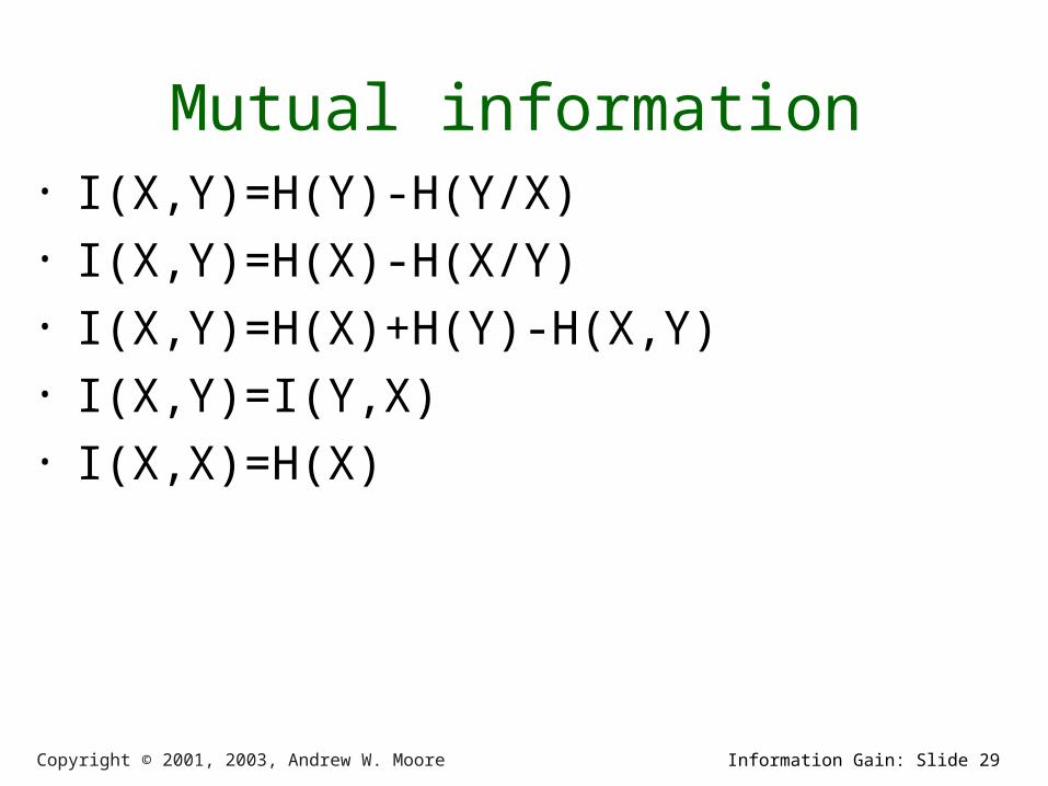
Axis-Aligned Gaussians

m

2

1

μ

m

m

2

12

32

22

12

0000

0000

0000

0000

0000

Σ

x1

x2

jiXX ii for


Spherical Gaussians

m

2

1

μ

2

2

2

2

2

0000

0000

0000

0000

0000

Σ

x1

x2

jiXX ii for


Subsets of variables

where as Write1)(

)(

1

2

1

m

um

um

m

X

X

X

X

X

X

X

V

U

V

UXX

This will be our standard notation for breaking an m-dimensional distribution into subsets of variables


Gaussian Marginals are

Gaussian

m

um

umm

X

X

X

X

X

X

X

1)(

)(

12

1

, where as Write VUV

UXX

THEN U is also distributed as a Gaussian

vvTuv

uvuu

v

u

ΣΣ

ΣΣ

μ

μ

V

U,N~ IF

uuu ΣμU ,N~

V

U Margin-alize

U



Gaussian

m

um

umm

X

X

X

X

X

X

X

1)(

)(

12

1


UXX


vvTuv

uvuu

v

u

ΣΣ

ΣΣ

μ

μ

V

U,N~ IF

uuu ΣμU ,N~

V

U Margin-alize

U

This fact is not immediately

obviousObvious, once we

know it’s a Gaussian (why?)



Gaussian

m

um

umm

X

X

X

X

X

X

X

1)(

)(

12

1


UXX


vvTuv

uvuu

v

u

ΣΣ

ΣΣ

μ

μ

V

U,N~ IF

uuu ΣμU ,N~

V

U Margin-alize

U

How would you prove this?

(snore...)

),(

)(

v

vvu

u

dp

p


Linear Transforms

remain Gaussian

ΣμX ,N~

Multiply AX X

Matrix A

Assume X is an m-dimensional Gaussian r.v.

Define Y to be a p-dimensional r. v. thusly (note ):

AXY

…where A is a p x m matrix. Then…

mp

TAAΣAμY ,N~


Adding samples of 2 independent Gaussians is

Gaussian

YXΣμYΣμX and ,N~ and ,N~ if yyxx

+ YX X Y

yxyx ΣΣμμYX ,N~ then

Why doesn’t this hold if X and Y are dependent?

Which of the below statements is true?

If X and Y are dependent, then X+Y is Gaussian but possibly with some other covariance

If X and Y are dependent, then X+Y might be non-Gaussian


Conditional of Gaussian is Gaussian

V

U Condition-alize

VU |

vvTuv

uvuu

v

u

ΣΣ

ΣΣ

μ

μ

V

U,N~ IF

where,N~ | THEN || vuvu ΣμVU

)( 1| vvv

Tuvuvu μVΣΣμμ

uvvvTuvuuvu ΣΣΣΣΣ 1

|


Caso Normal Bivariado

)(/ xyxy xy

x

)1( 222

/ yxy


vvTuv

uvuu

v

u

ΣΣ

ΣΣ

μ

μ

V

U,N~ IF


)( 1| vvv

Tuvuvu μVΣΣμμ


|

2

2

68.3967

967849,

76

2977N~ IF

y

w

where,N~ | THEN || ywywyw Σμ

2| 68.3

)76(9762977

yywμ

22

22

| 80868.3

967849 ywΣ


vvTuv

uvuu

v

u

ΣΣ

ΣΣ

μ

μ

V

U,N~ IF


)( 1| vvv

Tuvuvu μVΣΣμμ


|

2

2

68.3967

967849,

76

2977N~ IF

y

w


2| 68.3

)76(9762977

yywμ

22

22

| 80868.3

967849 ywΣ

P(w|m=82)

P(w|m=76)

P(w)


vvTuv

uvuu

v

u

ΣΣ

ΣΣ

μ

μ

V

U,N~ IF


)( 1| vvv

Tuvuvu μVΣΣμμ


|

2

2

68.3967

967849,

76

2977N~ IF

y

w


2| 68.3

)76(9762977

yywμ

22

22

| 80868.3

967849 ywΣ

P(w|m=82)

P(w|m=76)

P(w)

Note: conditional variance is

independent of the given value of v

Note: conditional variance can only be equal to or smaller

than marginal variance

Note: marginal mean is a linear function of

v

Note: when given value of v is v, the

conditional mean of u is u


Gaussians and the chain rule

vvT

vv

vvvuT

vv

ΣAΣ

AΣΣAAΣΣ

)( |

vvvvu ΣμVΣAVVU ,N~ and ,N~ | IF |

V

UChainRule

VU |V

Let A be a constant matrix

with,,N~ THEN ΣμV

U

v

v

μ

Aμμ


Available Gaussian tools

V

UChainRule

VU |V

V

U Condition-alize

VU |

+ YX X Y

Multiply AX X

Matrix A

V

U Margin-alize

U

vvTuv

uvuu

v

u

ΣΣ

ΣΣ

μ

μ

V

U,N~ IF uuu ΣμU ,N~ THEN

ΣμX ,N~ IF AXY AND TAAΣAμY ,N~ THEN

YXΣμYΣμX and ,N~ and ,N~ if yyxx

yxyx ΣΣμμYX ,N~ then


| where

vuvu || ,N~ | ΣμVUTHEN

vvTuv

uvuu

v

u

ΣΣ

ΣΣ

μ

μ

V

U,N~ IF

)( 1| vvv

Tuvuvu μVΣΣμμ

vvT

vv

vvvuT

vv

ΣAΣ

AΣΣAAΣΣ

)( |


with,,N~ THEN ΣμV

U


Assume…• You are an intellectual snob• You have a child


Intellectual snobs with children

• …are obsessed with IQ• In the world as a whole, IQs are drawn

from a Gaussian N(100,152)


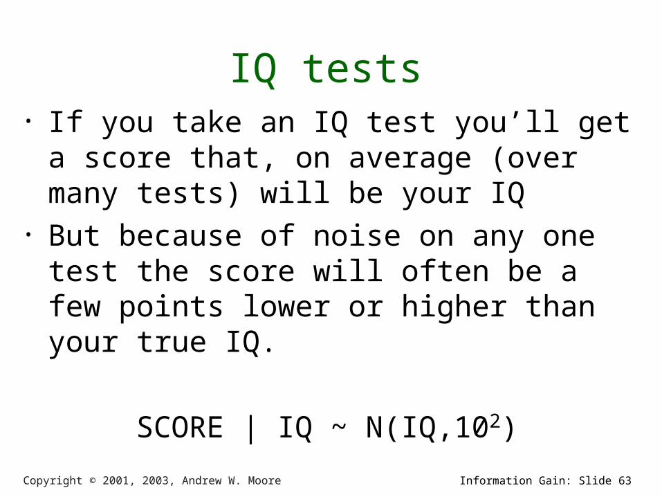
IQ tests• If you take an IQ test you’ll get a score

that, on average (over many tests) will be your IQ

• But because of noise on any one test the score will often be a few points lower or higher than your true IQ.

SCORE | IQ ~ N(IQ,102)


Assume…• You drag your kid off to get tested• She gets a score of 130• “Yippee” you screech and start deciding

how to casually refer to her membership of the top 2% of IQs in your Christmas newsletter.

P(X<130|=100,2=152) =

P(X<2| =0,2=1) =

erf(2) = 0.977


Assume…• You drag your kid off to get tested• She gets a score of 130• “Yippee” you screech and start deciding

how to casually refer to her membership of the top 2% of IQs in your Christmas newsletter.

P(X<130|=100,2=152) =

P(X<2| =0,2=1) =

erf(2) = 0.977

You are thinking:

Well sure the test isn’t accurate, so she might have

an IQ of 120 or she might have an 1Q of 140, but the most likely IQ given the evidence “score=130” is, of course,

130.

Can we trust this

reasoning?


What we really want:• IQ~N(100,152)• S|IQ ~ N(IQ,

102)• S=130

• Question: What is IQ | (S=130)?

Called the Posterior

Distribution of IQ


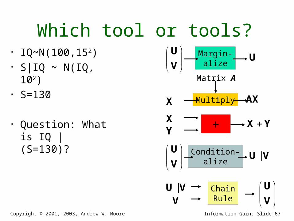
Which tool or tools?• IQ~N(100,152)• S|IQ ~ N(IQ,

102)• S=130


V

UChainRule

VU |V

V

U Condition-alize

VU |

+ YX X Y

Multiply AX X

Matrix A

V

U Margin-alize

U


Plan• IQ~N(100,152)• S|IQ ~ N(IQ,

102)• S=130


IQ

SChainRule

Q| ISIQ

S

IQ Condition-alize

SI |QSwap


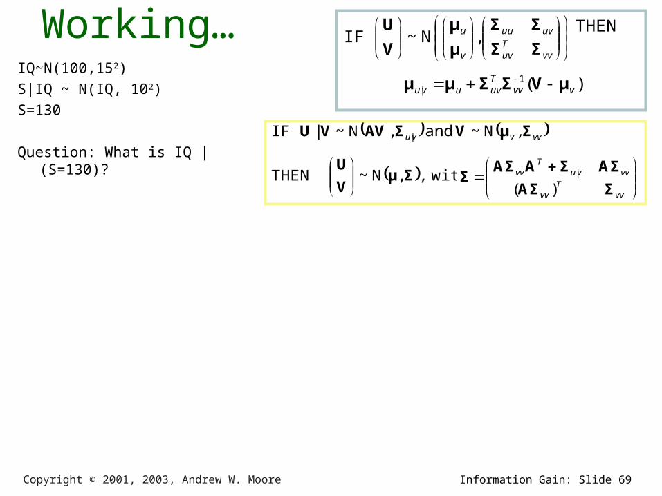
Working…IQ~N(100,152)S|IQ ~ N(IQ, 102)S=130

Question: What is IQ | (S=130)?

THEN

vvTuv

uvuu

v

u

ΣΣ

ΣΣ

μ

μ

V

U,N~ IF

)( 1| vvv

Tuvuvu μVΣΣμμ

vvT

vv

vvvuT

vv

ΣAΣ

AΣΣAAΣΣ

)( |


with,,N~ THEN ΣμV

U

Documents

Copyright © 2001, 2003, Andrew W. Moore Entropy and Information Gain Andrew W. Moore Professor School of Computer Science Carnegie Mellon University awm