Embed Size (px)
Citation preview
Copyright © Andrew W. Moore Slide 1
GaussiansAndrew W. Moore
ProfessorSchool of Computer ScienceCarnegie Mellon University
www.cs.cmu.edu/[email protected]
412-268-7599
Note to other teachers and users of these slides. Andrew would be delighted if you found this source material useful in giving your own lectures. Feel free to use these slides verbatim, or to modify them to fit your own needs. PowerPoint originals are available. If you make use of a significant portion of these slides in your own lecture, please include this message, or the following link to the source repository of Andrew’s tutorials: http://www.cs.cmu.edu/~awm/tutorials . Comments and corrections gratefully received.
Copyright © Andrew W. Moore Slide 2
Gaussians in Data Mining• Why we should care• The entropy of a PDF• Univariate Gaussians• Multivariate Gaussians• Bayes Rule and Gaussians• Maximum Likelihood and MAP using
Gaussians
Copyright © Andrew W. Moore Slide 3
Why we should care• Gaussians are as natural as Orange Juice
and Sunshine• We need them to understand Bayes
Optimal Classifiers• We need them to understand regression• We need them to understand neural nets• We need them to understand mixture
models• …
(You get the idea)

Copyright © Andrew W. Moore Slide 4
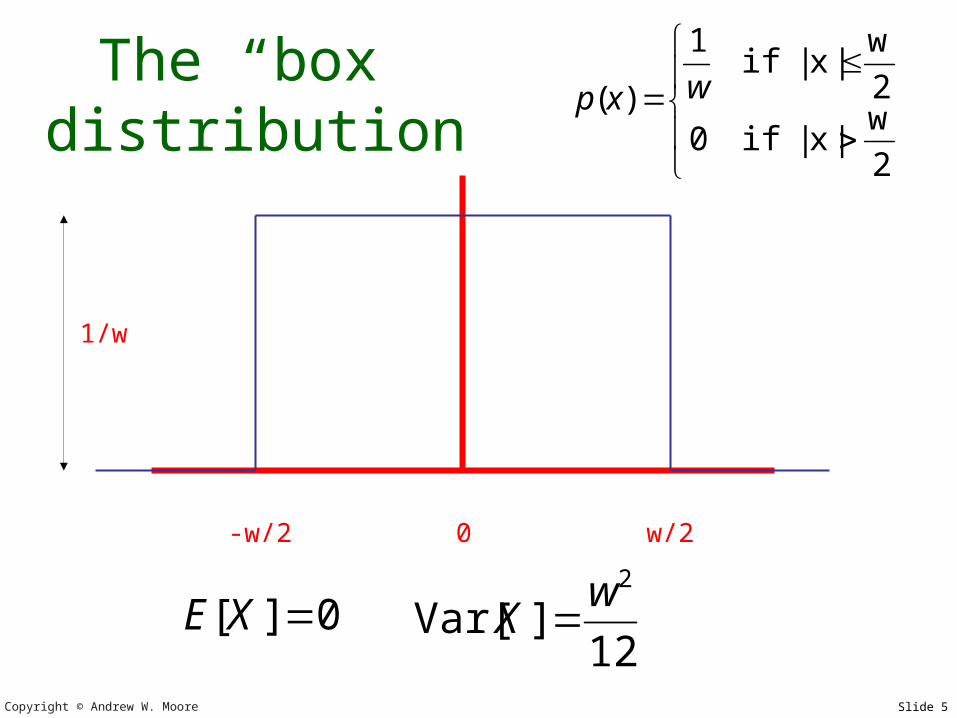
The “box” distribution
-w/2 0 w/2
1/w
2
w|x|if0
2
w|x|if
1
)( wxp
Copyright © Andrew W. Moore Slide 5
The “box” distribution
-w/2 0 w/2
1/w
0][ XE12
]Var[2w
X
2
w|x|if0
2
w|x|if
1
)( wxp

Copyright © Andrew W. Moore Slide 6
Entropy of a PDF
x
dxxpxpXHX )(log)(][ ofEntropy
Natural log (ln or loge)
The larger the entropy of a distribution…
…the harder it is to predict
…the harder it is to compress it
…the less spiky the distribution
Copyright © Andrew W. Moore Slide 7
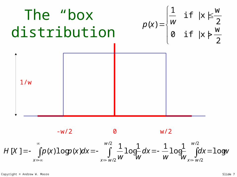
The “box” distribution
-w/2 0 w/2
1/w
2
w|x|if0
2
w|x|if
1
)( wxp
wdxww
dxww
dxxpxpXHw
wx
w
wxx
log1
log11
log1
)(log)(][2/
2/
2/
2/
Copyright © Andrew W. Moore Slide 8
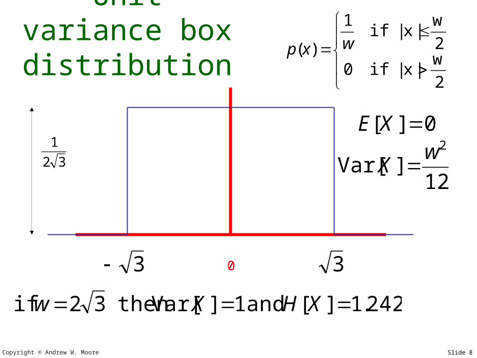
Unit variance box
distribution
0
12]Var[
2wX
0][ XE
242.1][ and 1]Var[ then 32 if XHXw
3
32
1
3
2
w|x|if0
2
w|x|if
1
)( wxp
Copyright © Andrew W. Moore Slide 9
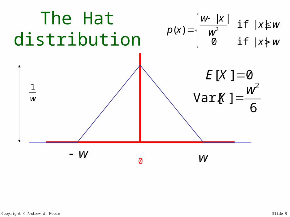
The Hat distribution
0
w|x|
w|x|w
xwxp
if0
if||
)( 2
6]Var[
2wX
0][ XE
w
1
w
w
Copyright © Andrew W. Moore Slide 10
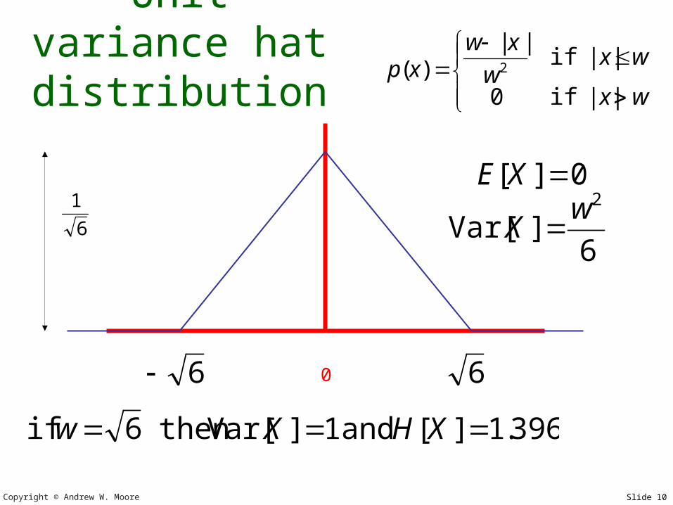
Unit variance hat
distribution
0
w|x|
w|x|w
xwxp
if0
if||
)( 2
6]Var[
2wX
0][ XE
396.1][ and 1]Var[ then 6 if XHXw
6
6
1
6
Copyright © Andrew W. Moore Slide 11
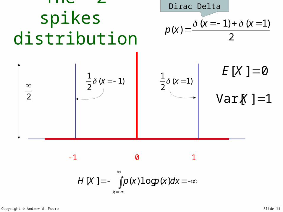
The “2 spikes” distribution
-1 0 1
2
)1()1()(
xxxp
x
dxxpxpXH )(log)(][
1]Var[ X
0][ XE
2
)1(2
1x )1(
2
1x
Dirac Delta
Copyright © Andrew W. Moore Slide 12
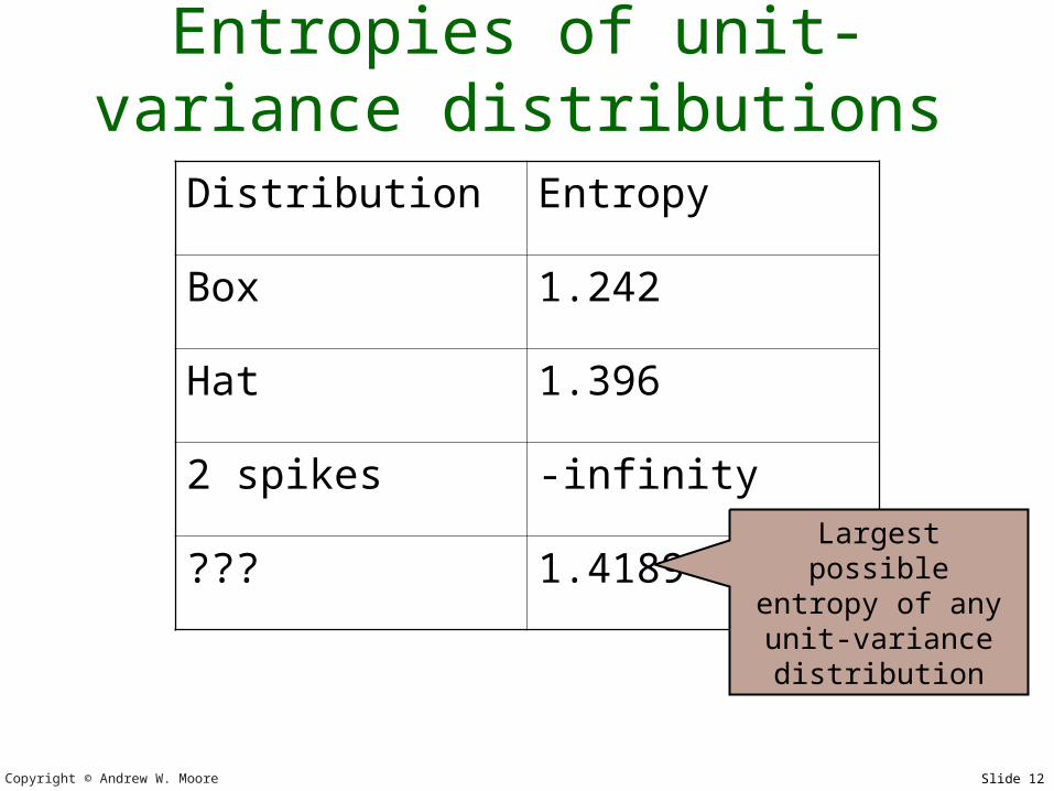
Entropies of unit-variance distributions
Distribution Entropy
Box 1.242
Hat 1.396
2 spikes -infinity
??? 1.4189 Largest possible entropy of any unit-variance distribution
Copyright © Andrew W. Moore Slide 13
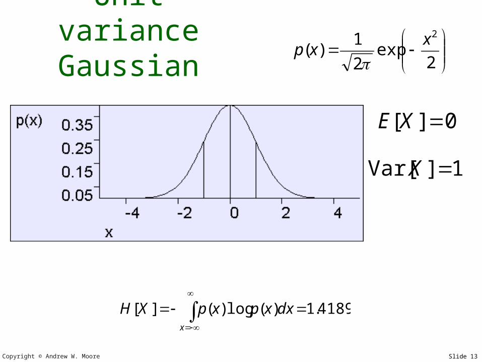
Unit variance Gaussian
2exp
2
1)(
2xxp
4189.1)(log)(][
x
dxxpxpXH
1]Var[ X
0][ XE
Copyright © Andrew W. Moore Slide 14
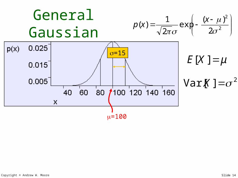
General Gaussian
2
2
2
)(exp
2
1)(
x
xp
2]Var[ X
μXE ][
=100
=15
Copyright © Andrew W. Moore Slide 15
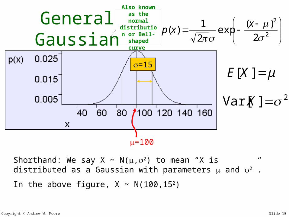
General Gaussian
2
2
2
)(exp
2
1)(
x
xp
2]Var[ X
μXE ][
=100
=15
Shorthand: We say X ~ N(,2) to mean “X is distributed as a Gaussian with parameters and 2”.
In the above figure, X ~ N(100,152)
Also known as the normal
distribution or Bell-shaped curve

Copyright © Andrew W. Moore Slide 16
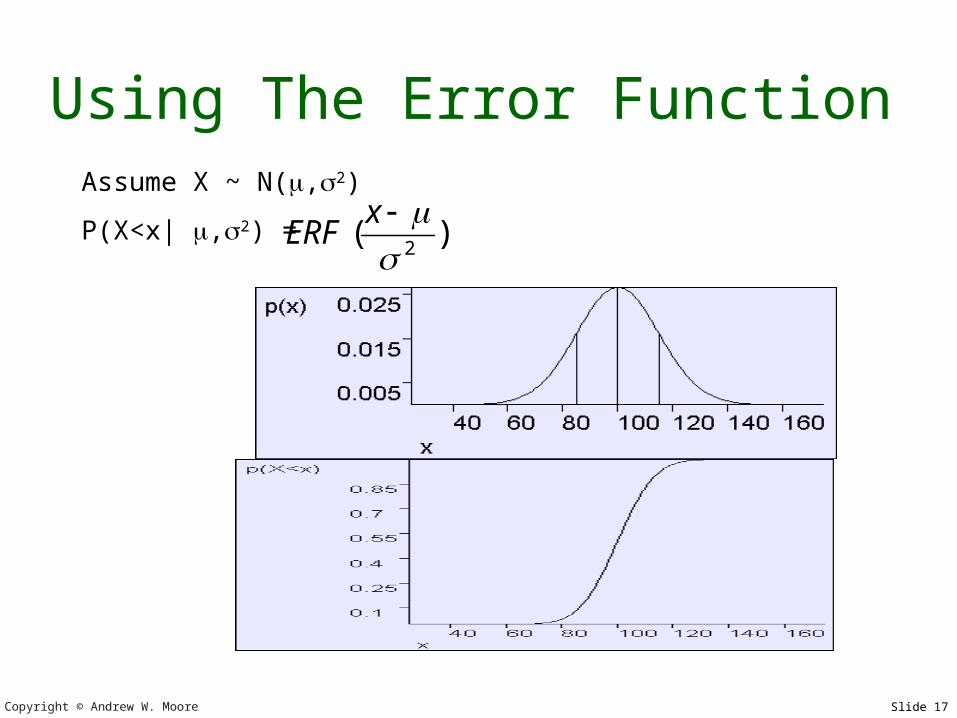
The Error FunctionAssume X ~ N(0,1)
Define ERF(x) = P(X<x) = Cumulative Distribution of X
x
z
dzzpxERF )()(
x
z
dzz
2exp
2
1 2
Copyright © Andrew W. Moore Slide 17
Using The Error FunctionAssume X ~ N(,2)
P(X<x| ,2) = )(2x
ERF
Copyright © Andrew W. Moore Slide 18
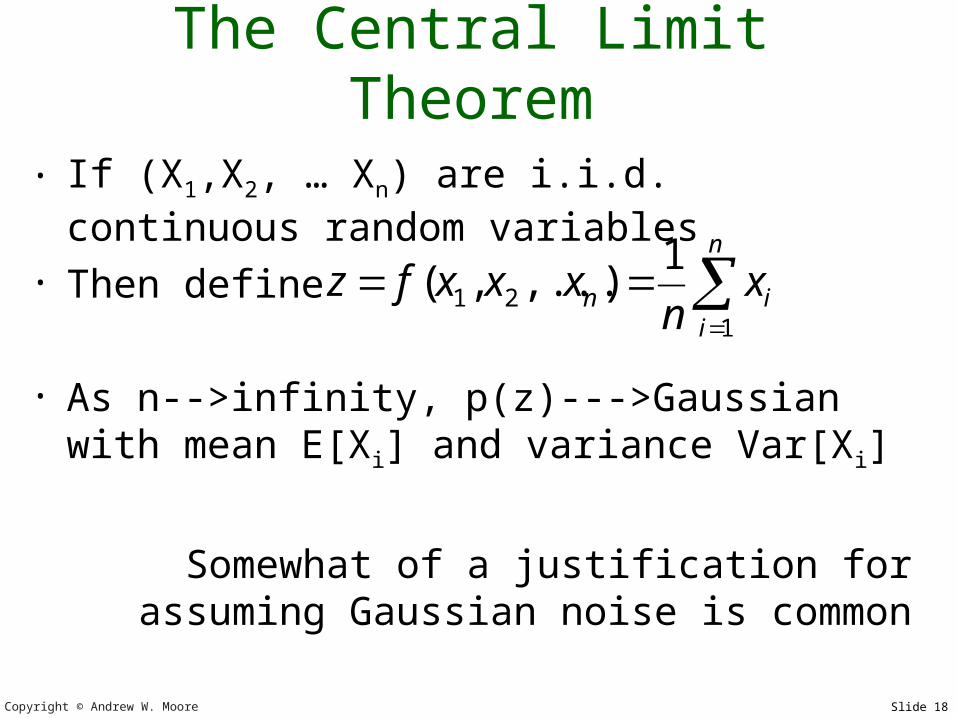
The Central Limit Theorem• If (X1,X2, … Xn) are i.i.d. continuous
random variables• Then define
• As n-->infinity, p(z)--->Gaussian with mean E[Xi] and variance Var[Xi]
Somewhat of a justification for assuming Gaussian noise is common
n
iin x
nxxxfz
121
1),...,(
Copyright © Andrew W. Moore Slide 19
Other amazing facts about Gaussians
• Wouldn’t you like to know?
• We will not examine them until we need to.
Copyright © Andrew W. Moore Slide 20
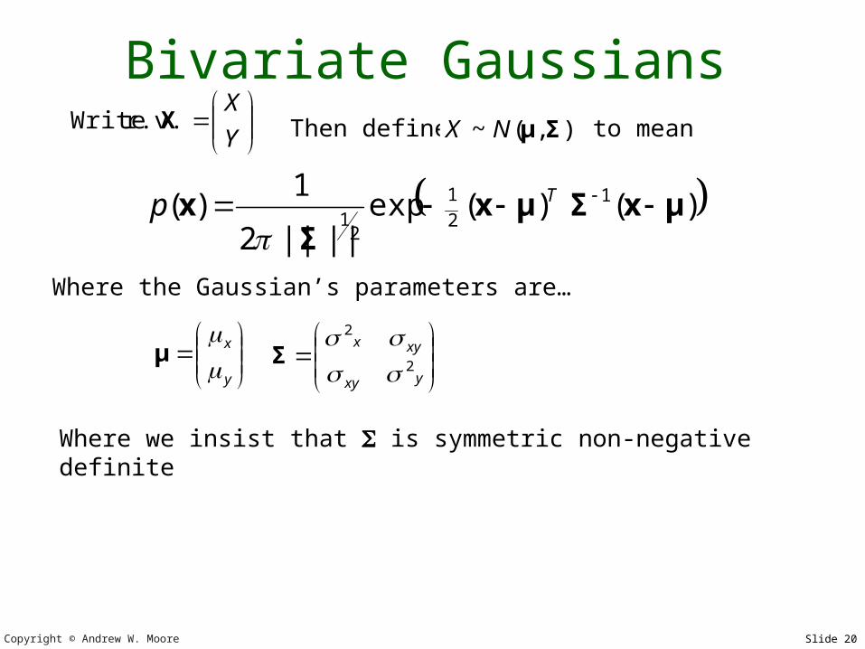
Bivariate Gaussians
)()(exp||||2
1)( 1
2
1
21 μxΣμx
Σx Tp
y
x
μ
Y
X X r.v. Write
yxy
xyx
2
2
Σ
Then define ),(~ ΣμNX to mean
Where the Gaussian’s parameters are…
Where we insist that is symmetric non-negative definite
Copyright © Andrew W. Moore Slide 21
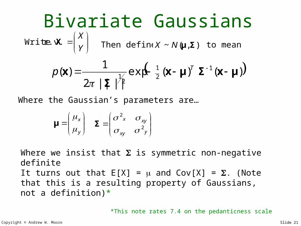
Bivariate Gaussians
)()(exp||||2
1)( 1
2
1
21 μxΣμx
Σx Tp
y
x
μ
Y
X X r.v. Write
yxy
xyx
2
2
Σ
Then define ),(~ ΣμNX to mean
Where the Gaussian’s parameters are…
Where we insist that is symmetric non-negative definite
It turns out that E[X] = and Cov[X] = . (Note that this is a resulting property of Gaussians, not a definition)*
*This note rates 7.4 on the pedanticness scale
Copyright © Andrew W. Moore Slide 22
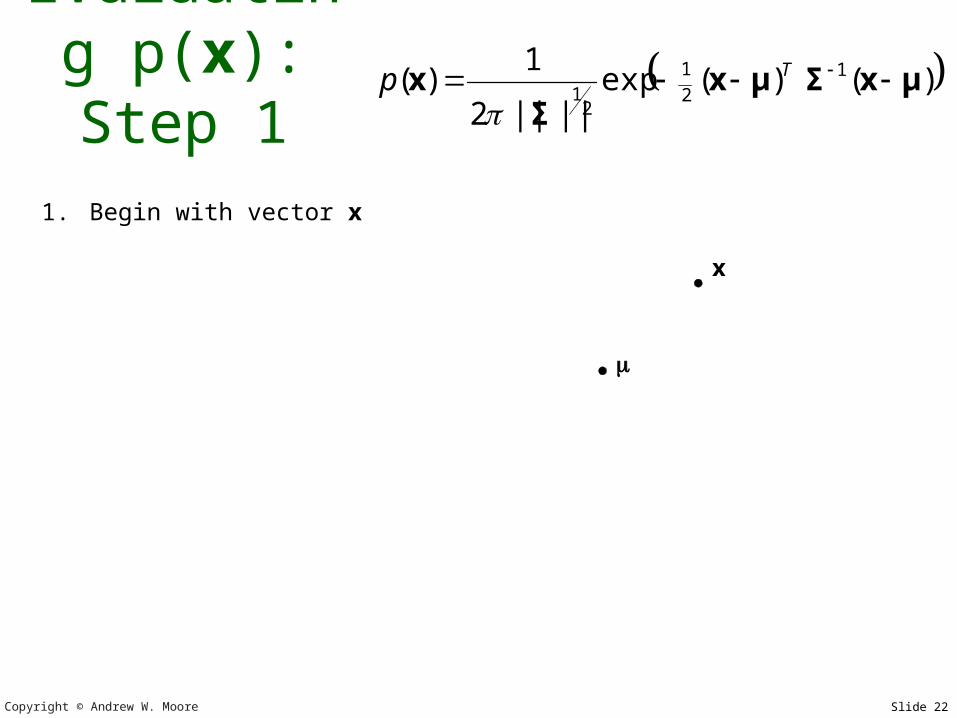
Evaluating p(x): Step
1 )()(exp
||||2
1)( 1
2
1
21 μxΣμx
Σx Tp
1. Begin with vector x
x
Copyright © Andrew W. Moore Slide 23
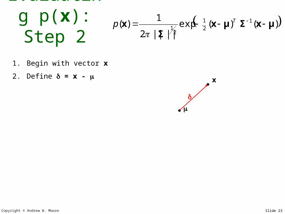
Evaluating p(x): Step
21. Begin with vector x
2. Define = x - x
)()(exp||||2
1)( 1
2
1
21 μxΣμx
Σx Tp
Copyright © Andrew W. Moore Slide 24
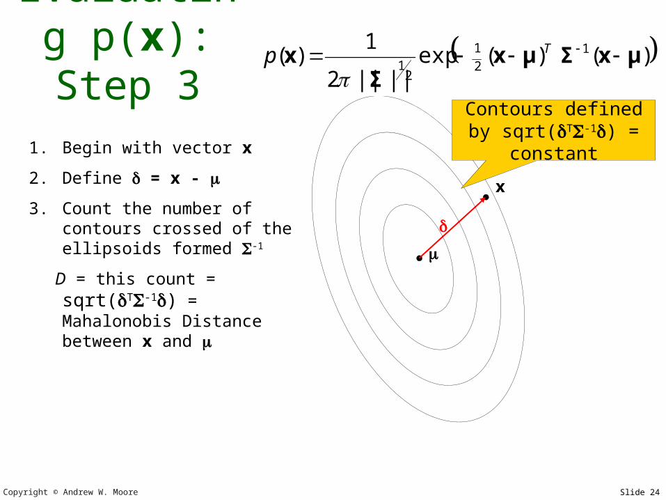
Evaluating p(x): Step
31. Begin with vector x
2. Define = x -
3. Count the number of contours crossed of the ellipsoids formed -1
D = this count = sqrt(T-
1) = Mahalonobis Distance between x and
x
Contours defined by sqrt(T-1) =
constant
)()(exp||||2
1)( 1
2
1
21 μxΣμx
Σx Tp
Copyright © Andrew W. Moore Slide 25
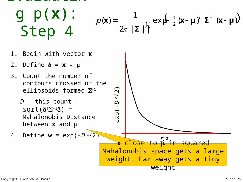
Evaluating p(x): Step
41. Begin with vector x
2. Define = x -
3. Count the number of contours crossed of the ellipsoids formed -1
D = this count = sqrt(T-
1) = Mahalonobis Distance between x and
4. Define w = exp(-D 2/2)
D 2
exp(-
D 2
/2)
x close to in squared Mahalonobis space gets a large weight. Far away
gets a tiny weight
)()(exp||||2
1)( 1
2
1
21 μxΣμx
Σx Tp
Copyright © Andrew W. Moore Slide 26
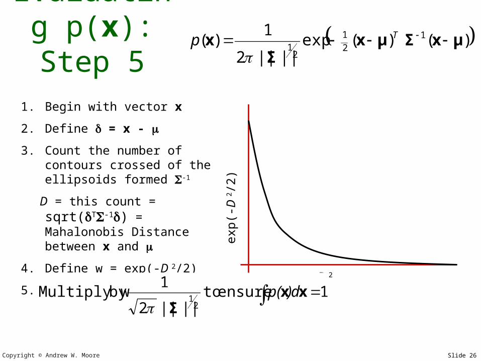
Evaluating p(x): Step
51. Begin with vector x
2. Define = x -
3. Count the number of contours crossed of the ellipsoids formed -1
D = this count = sqrt(T-
1) = Mahalonobis Distance between x and
4. Define w = exp(-D 2/2)
5. D 2
exp(-
D 2
/2)
1ensure to||||2
1by Multiply w
21 xx
Σd)p(
)()(exp||||2
1)( 1
2
1
21 μxΣμx
Σx Tp
Copyright © Andrew W. Moore Slide 27
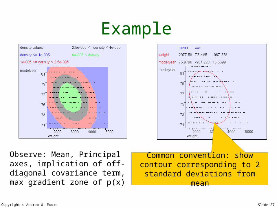
Example
Common convention: show contour corresponding to 2
standard deviations from mean
Observe: Mean, Principal axes, implication of off-diagonal covariance term, max gradient zone of p(x)
Copyright © Andrew W. Moore Slide 28
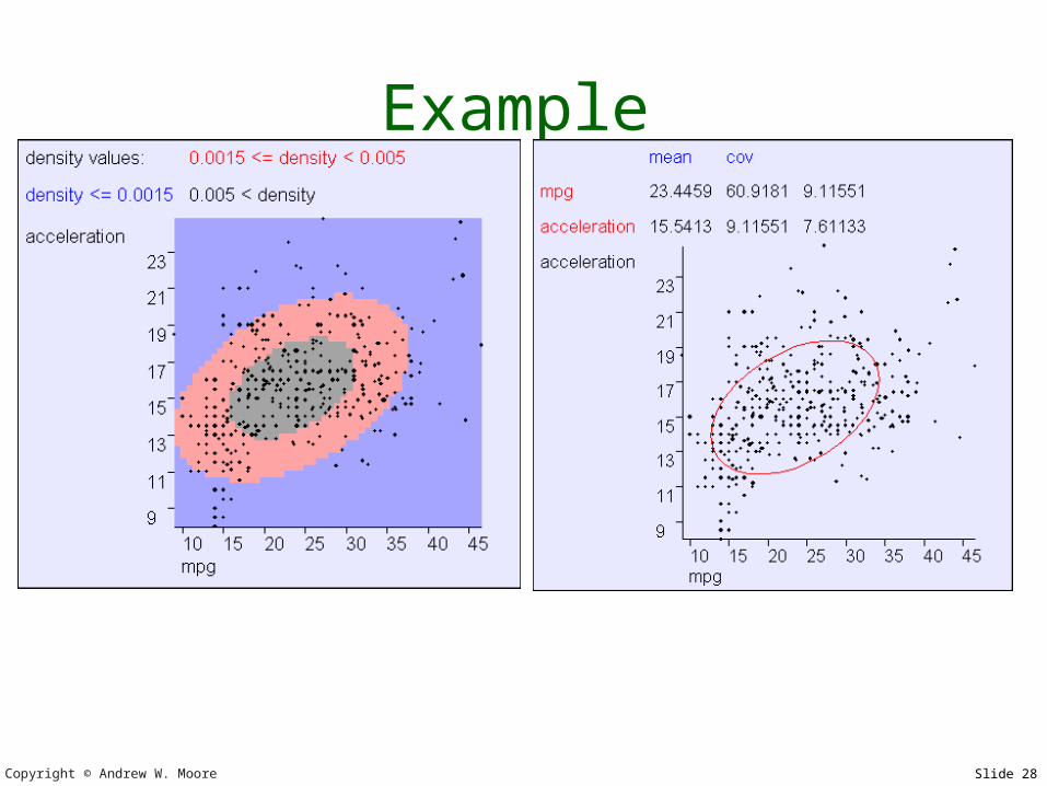
Example
Copyright © Andrew W. Moore Slide 29
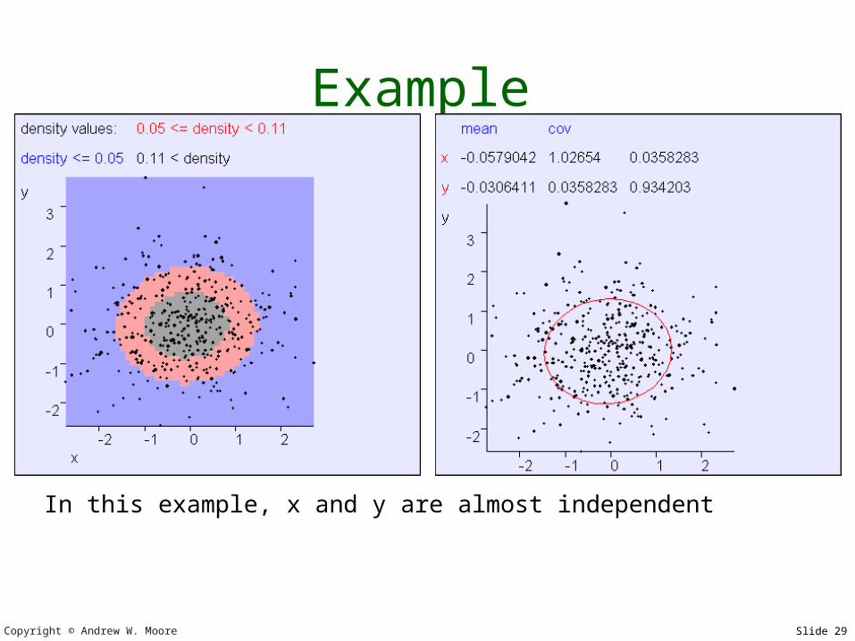
Example
In this example, x and y are almost independent
Copyright © Andrew W. Moore Slide 30
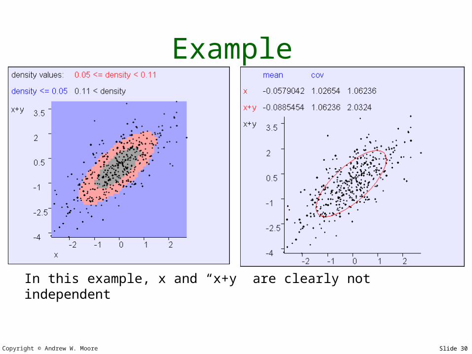
Example
In this example, x and “x+y” are clearly not independent
Copyright © Andrew W. Moore Slide 31
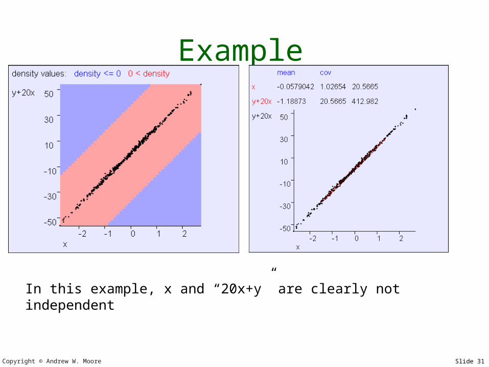
Example
In this example, x and “20x+y” are clearly not independent
Copyright © Andrew W. Moore Slide 32
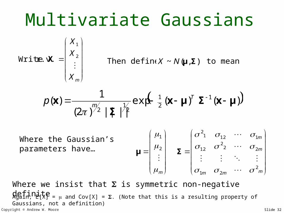
Multivariate Gaussians
)()(exp||||)2(
1)( 1
2
1
21
2μxΣμx
Σx T
mp
m
2
1
μ
mX
X
X
2
1
r.v. Write X
mmm
m
m
221
222
12
11212
Σ
Then define ),(~ ΣμNX to mean
Where the Gaussian’s parameters have…
Where we insist that is symmetric non-negative definite
Again, E[X] = and Cov[X] = . (Note that this is a resulting property of Gaussians, not a definition)

Copyright © Andrew W. Moore Slide 33
General Gaussians
m
2
1
μ
mmm
m
m
221
222
12
11212
Σ
x1
x2

Copyright © Andrew W. Moore Slide 34
Axis-Aligned Gaussians
m
2
1
μ
m
m
2
12
32
22
12
0000
0000
0000
0000
0000
Σ
x1
x2
jiXX ii for

Copyright © Andrew W. Moore Slide 35
Spherical Gaussians
m
2
1
μ
2
2
2
2
2
0000
0000
0000
0000
0000
Σ
x1
x2
jiXX ii for
Copyright © Andrew W. Moore Slide 36
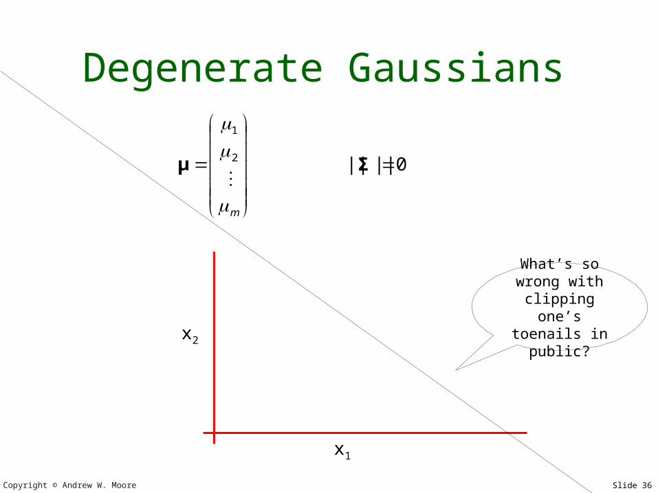
Degenerate Gaussians
m
2
1
μ 0|||| Σ
x1
x2
What’s so wrong with
clipping one’s toenails in
public?

Copyright © Andrew W. Moore Slide 37
Where are we now?• We’ve seen the formulae for Gaussians• We have an intuition of how they
behave• We have some experience of “reading”
a Gaussian’s covariance matrix
• Coming next:Some useful tricks with Gaussians
Copyright © Andrew W. Moore Slide 38
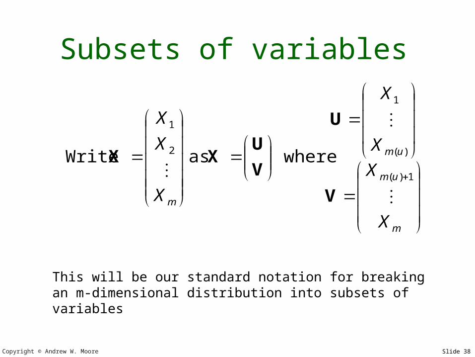
Subsets of variables
where as Write1)(
)(
1
2
1
m
um
um
m
X
X
X
X
X
X
X
V
U
V
UXX
This will be our standard notation for breaking an m-dimensional distribution into subsets of variables
Copyright © Andrew W. Moore Slide 39
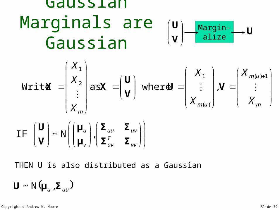
Gaussian Marginals are
Gaussian
m
um
umm
X
X
X
X
X
X
X
1)(
)(
12
1
, where as Write VUV
UXX
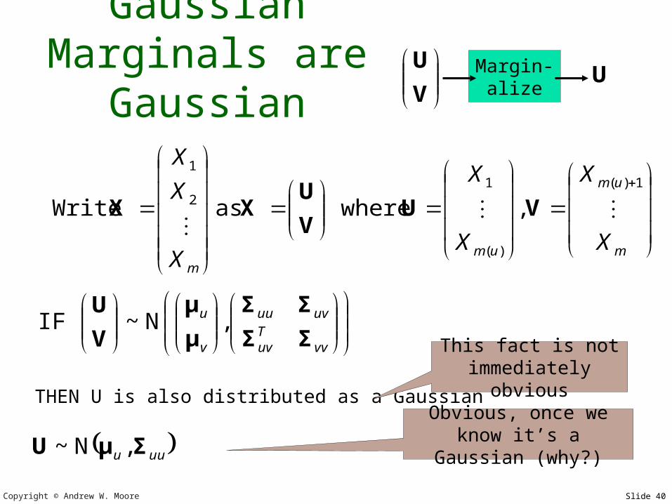
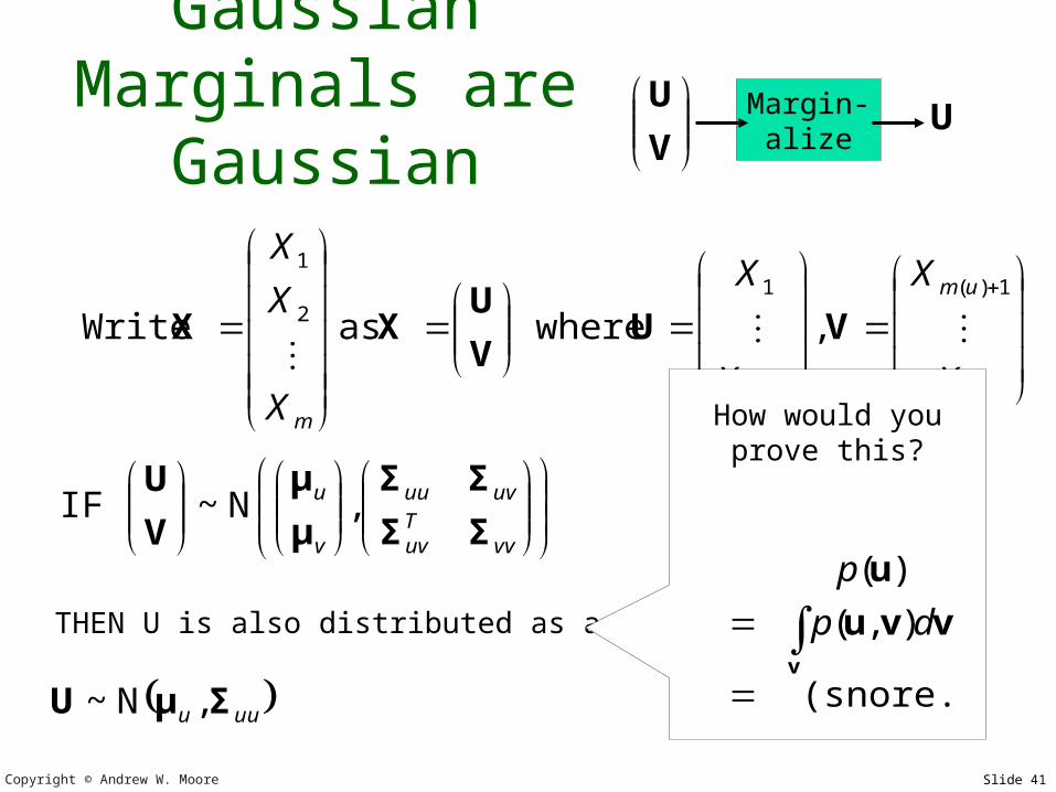
THEN U is also distributed as a Gaussian
vvTuv
uvuu
v
u
ΣΣ
ΣΣ
μ
μ
V
U,N~ IF
uuu ΣμU ,N~
V
U Margin-alize
U
Copyright © Andrew W. Moore Slide 40
Gaussian Marginals are
Gaussian
m
um
umm
X
X
X
X
X
X
X
1)(
)(
12
1
, where as Write VUV
UXX
THEN U is also distributed as a Gaussian
vvTuv
uvuu
v
u
ΣΣ
ΣΣ
μ
μ
V
U,N~ IF
uuu ΣμU ,N~
V
U Margin-alize
U
This fact is not immediately
obviousObvious, once we
know it’s a Gaussian (why?)
Copyright © Andrew W. Moore Slide 41
Gaussian Marginals are
Gaussian
m
um
umm
X
X
X
X
X
X
X
1)(
)(
12
1
, where as Write VUV
UXX
THEN U is also distributed as a Gaussian
vvTuv
uvuu
v
u
ΣΣ
ΣΣ
μ
μ
V
U,N~ IF
uuu ΣμU ,N~
V
U Margin-alize
U
How would you prove this?
(snore...)
),(
)(
v
vvu
u
dp
p
Copyright © Andrew W. Moore Slide 42
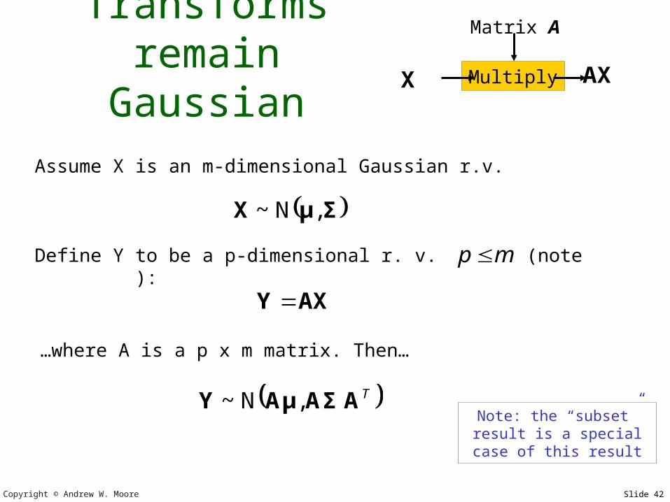
Linear Transforms
remain Gaussian
ΣμX ,N~
Multiply AX X
Matrix A
Assume X is an m-dimensional Gaussian r.v.
Define Y to be a p-dimensional r. v. thusly (note ):
AXY
…where A is a p x m matrix. Then…
mp
TAAΣAμY ,N~ Note: the “subset”
result is a special case of this result
Copyright © Andrew W. Moore Slide 43
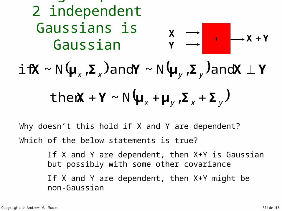
Adding samples of 2 independent Gaussians is
Gaussian
YXΣμYΣμX and ,N~ and ,N~ if yyxx
+ YX X Y
yxyx ΣΣμμYX ,N~ then
Why doesn’t this hold if X and Y are dependent?
Which of the below statements is true?
If X and Y are dependent, then X+Y is Gaussian but possibly with some other covariance
If X and Y are dependent, then X+Y might be non-Gaussian
Copyright © Andrew W. Moore Slide 44
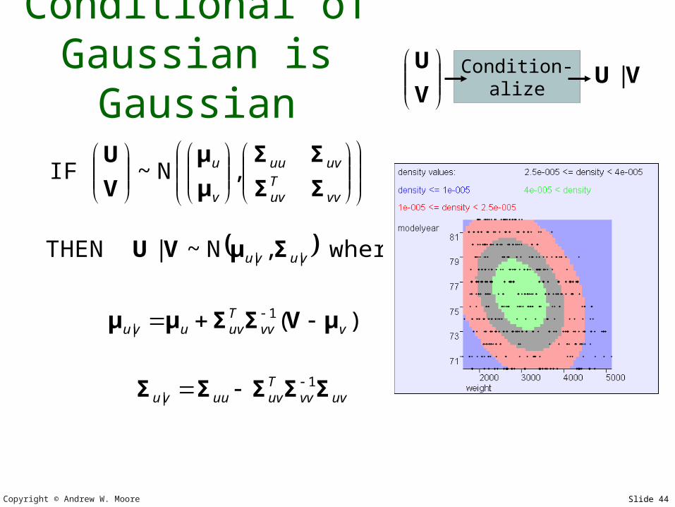
Conditional of Gaussian is Gaussian
V
U Condition-alize
VU |
vvTuv
uvuu
v
u
ΣΣ
ΣΣ
μ
μ
V
U,N~ IF
where,N~ | THEN || vuvu ΣμVU
)( 1| vvv
Tuvuvu μVΣΣμμ
uvvvTuvuuvu ΣΣΣΣΣ 1
|

Copyright © Andrew W. Moore Slide 45
vvTuv
uvuu
v
u
ΣΣ
ΣΣ
μ
μ
V
U,N~ IF
where,N~ | THEN || vuvu ΣμVU
)( 1| vvv
Tuvuvu μVΣΣμμ
uvvvTuvuuvu ΣΣΣΣΣ 1
|
2
2
68.3967
967849,
76
2977N~ IF
y
w
where,N~ | THEN || ywywyw Σμ
2| 68.3
)76(9762977
yywμ
22
22
| 80868.3
967849 ywΣ

Copyright © Andrew W. Moore Slide 46
vvTuv
uvuu
v
u
ΣΣ
ΣΣ
μ
μ
V
U,N~ IF
where,N~ | THEN || vuvu ΣμVU
)( 1| vvv
Tuvuvu μVΣΣμμ
uvvvTuvuuvu ΣΣΣΣΣ 1
|
2
2
68.3967
967849,
76
2977N~ IF
y
w
where,N~ | THEN || ywywyw Σμ
2| 68.3
)76(9762977
yywμ
22
22
| 80868.3
967849 ywΣ
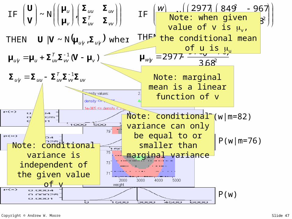
P(w|m=82)
P(w|m=76)
P(w)
Copyright © Andrew W. Moore Slide 47
vvTuv
uvuu
v
u
ΣΣ
ΣΣ
μ
μ
V
U,N~ IF
where,N~ | THEN || vuvu ΣμVU
)( 1| vvv
Tuvuvu μVΣΣμμ
uvvvTuvuuvu ΣΣΣΣΣ 1
|
2
2
68.3967
967849,
76
2977N~ IF
y
w
where,N~ | THEN || ywywyw Σμ
2| 68.3
)76(9762977
yywμ
22
22
| 80868.3
967849 ywΣ
P(w|m=82)
P(w|m=76)
P(w)
Note: conditional variance is
independent of the given value of v
Note: conditional variance can only be equal to or smaller
than marginal variance
Note: marginal mean is a linear function of
v
Note: when given value of v is v, the
conditional mean of u is u
Copyright © Andrew W. Moore Slide 48
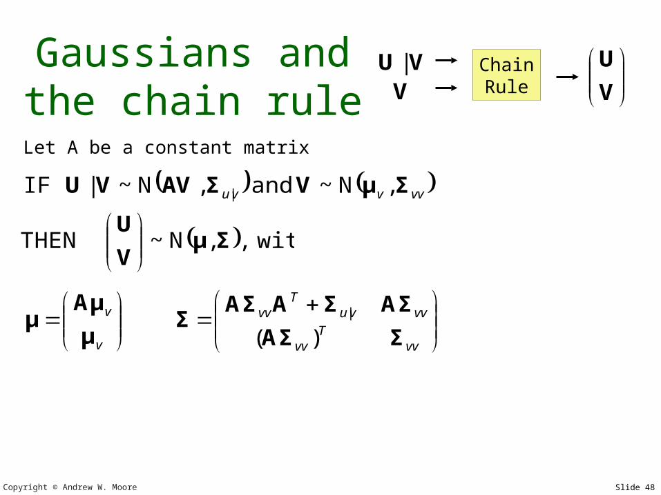
Gaussians and the chain rule
vvT
vv
vvvuT
vv
ΣAΣ
AΣΣAAΣΣ
)( |
vvvvu ΣμVΣAVVU ,N~ and ,N~ | IF |
V
UChainRule
VU |V
Let A be a constant matrix
with,,N~ THEN ΣμV
U
v
v
μ
Aμμ

Copyright © Andrew W. Moore Slide 49
Available Gaussian tools
V
UChainRule
VU |V
V
U Condition-alize
VU |
+ YX X Y
Multiply AX X
Matrix A
V
U Margin-alize
U
vvTuv
uvuu
v
u
ΣΣ
ΣΣ
μ
μ
V
U,N~ IF uuu ΣμU ,N~ THEN
ΣμX ,N~ IF AXY AND TAAΣAμY ,N~ THEN
YXΣμYΣμX and ,N~ and ,N~ if yyxx
yxyx ΣΣμμYX ,N~ then
uvvvTuvuuvu ΣΣΣΣΣ 1
| where
vuvu || ,N~ | ΣμVUTHEN
vvTuv
uvuu
v
u
ΣΣ
ΣΣ
μ
μ
V
U,N~ IF
)( 1| vvv
Tuvuvu μVΣΣμμ
vvT
vv
vvvuT
vv
ΣAΣ
AΣΣAAΣΣ
)( |
vvvvu ΣμVΣAVVU ,N~ and ,N~ | IF |
with,,N~ THEN ΣμV
U

Copyright © Andrew W. Moore Slide 50
Assume…• You are an intellectual snob• You have a child

Copyright © Andrew W. Moore Slide 51
Intellectual snobs with children
• …are obsessed with IQ• In the world as a whole, IQs are drawn
from a Gaussian N(100,152)
Copyright © Andrew W. Moore Slide 52
IQ tests• If you take an IQ test you’ll get a score
that, on average (over many tests) will be your IQ
• But because of noise on any one test the score will often be a few points lower or higher than your true IQ.
SCORE | IQ ~ N(IQ,102)
Copyright © Andrew W. Moore Slide 53
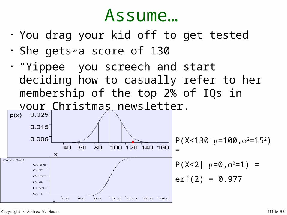
Assume…• You drag your kid off to get tested• She gets a score of 130• “Yippee” you screech and start deciding
how to casually refer to her membership of the top 2% of IQs in your Christmas newsletter.
P(X<130|=100,2=152) =
P(X<2| =0,2=1) =
erf(2) = 0.977
Copyright © Andrew W. Moore Slide 54
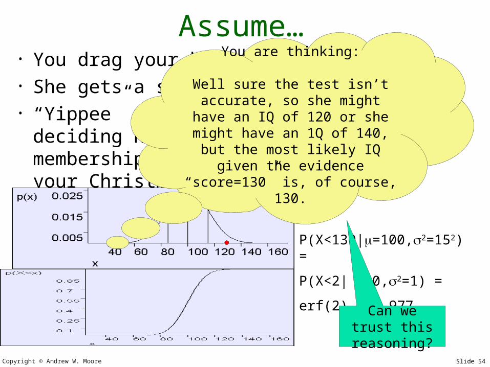
Assume…• You drag your kid off to get tested• She gets a score of 130• “Yippee” you screech and start deciding
how to casually refer to her membership of the top 2% of IQs in your Christmas newsletter.
P(X<130|=100,2=152) =
P(X<2| =0,2=1) =
erf(2) = 0.977
You are thinking:
Well sure the test isn’t accurate, so she might have
an IQ of 120 or she might have an 1Q of 140, but the most likely IQ given the evidence “score=130” is, of course,
130.
Can we trust this
reasoning?
Copyright © Andrew W. Moore Slide 55
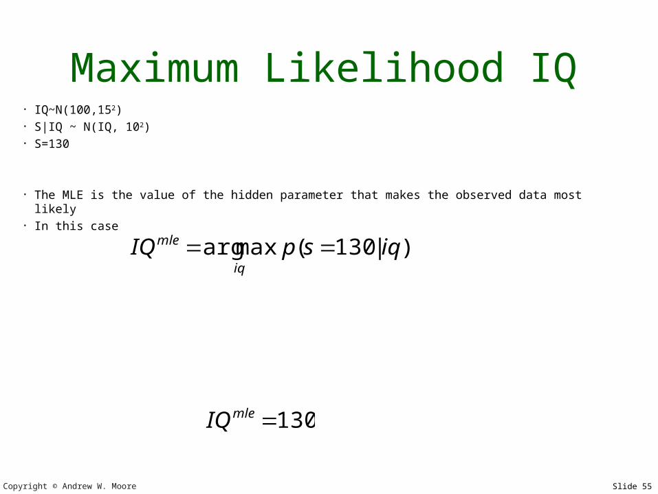
Maximum Likelihood IQ• IQ~N(100,152)• S|IQ ~ N(IQ, 102)• S=130
• The MLE is the value of the hidden parameter that makes the observed data most likely• In this case
)|130(maxarg iqspIQiq
mle
130 mleIQ
Copyright © Andrew W. Moore Slide 56
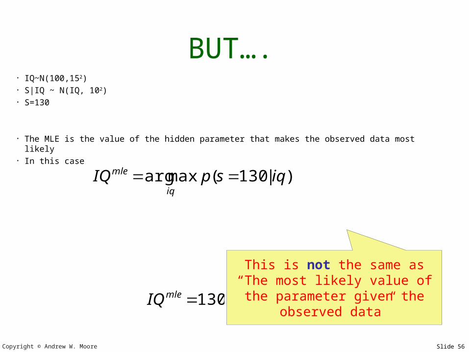
BUT….• IQ~N(100,152)• S|IQ ~ N(IQ, 102)• S=130
• The MLE is the value of the hidden parameter that makes the observed data most likely• In this case
)|130(maxarg iqspIQiq
mle
130 mleIQ
This is not the same as“The most likely value of the
parameter given the observed data”
Copyright © Andrew W. Moore Slide 57
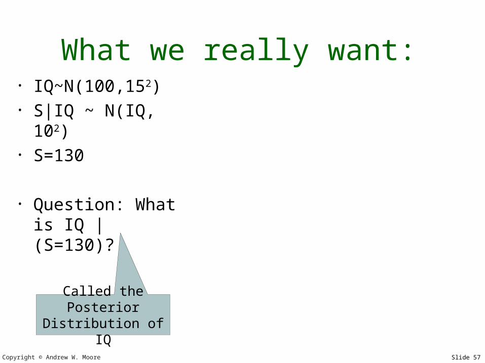
What we really want:• IQ~N(100,152)• S|IQ ~ N(IQ,
102)• S=130
• Question: What is IQ | (S=130)?
Called the Posterior
Distribution of IQ
Copyright © Andrew W. Moore Slide 58
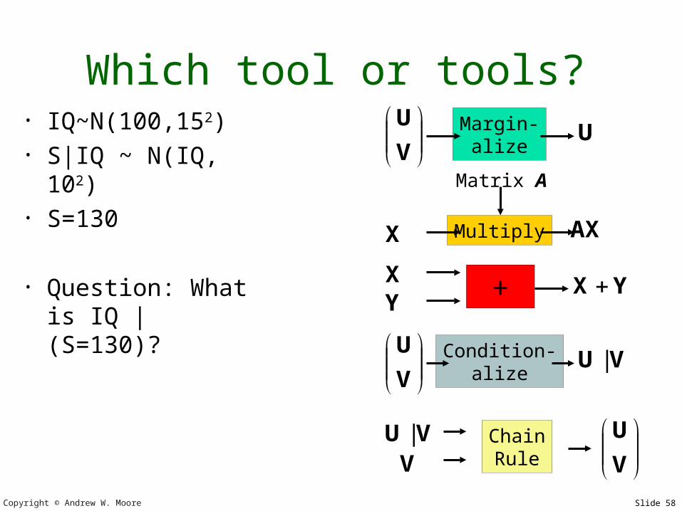
Which tool or tools?• IQ~N(100,152)• S|IQ ~ N(IQ,
102)• S=130
• Question: What is IQ | (S=130)?
V
UChainRule
VU |V
V
U Condition-alize
VU |
+ YX X Y
Multiply AX X
Matrix A
V
U Margin-alize
U
Copyright © Andrew W. Moore Slide 59
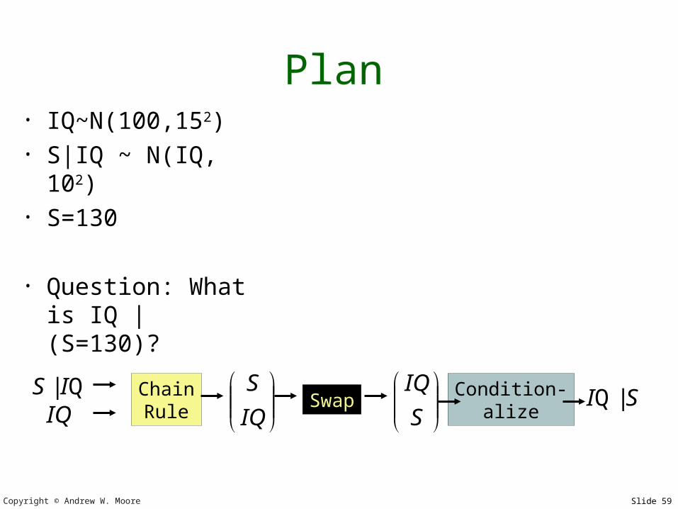
Plan• IQ~N(100,152)• S|IQ ~ N(IQ,
102)• S=130
• Question: What is IQ | (S=130)?
IQ
SChainRule
Q| ISIQ
S
IQ Condition-alize
SI |QSwap
Copyright © Andrew W. Moore Slide 60
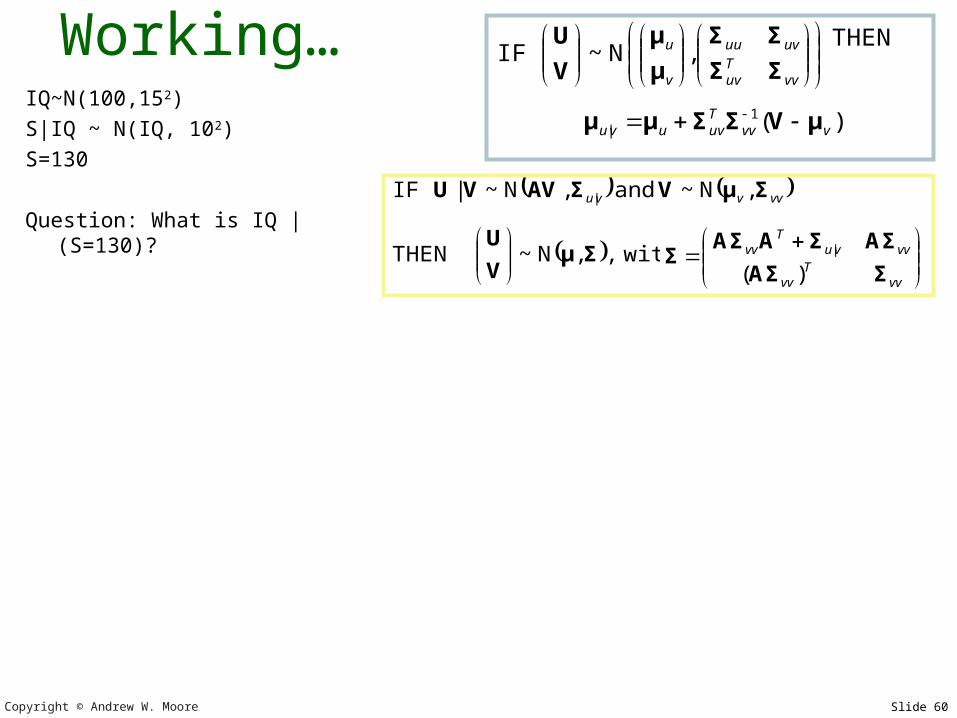
Working…IQ~N(100,152)S|IQ ~ N(IQ, 102)S=130
Question: What is IQ | (S=130)?
THEN
vvTuv
uvuu
v
u
ΣΣ
ΣΣ
μ
μ
V
U,N~ IF
)( 1| vvv
Tuvuvu μVΣΣμμ
vvT
vv
vvvuT
vv
ΣAΣ
AΣΣAAΣΣ
)( |
vvvvu ΣμVΣAVVU ,N~ and ,N~ | IF |
with,,N~ THEN ΣμV
U
Copyright © Andrew W. Moore Slide 61
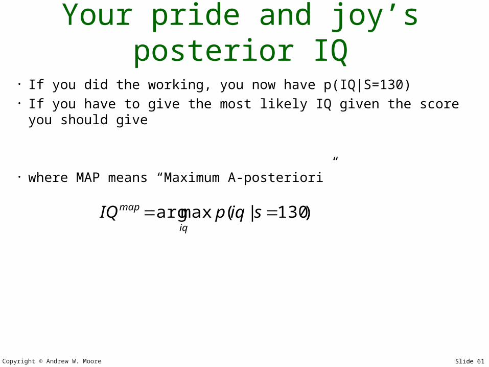
Your pride and joy’s posterior IQ
• If you did the working, you now have p(IQ|S=130)• If you have to give the most likely IQ given the score you
should give
• where MAP means “Maximum A-posteriori”
)130|(maxarg siqpIQiq
map
Copyright © Andrew W. Moore Slide 62
What you should know• The Gaussian PDF formula off by heart• Understand the workings of the
formula for a Gaussian• Be able to understand the Gaussian
tools described so far• Have a rough idea of how you could
prove them• Be happy with how you could use them