Embed Size (px)
Citation preview

Oct 15th, 2001Copyright © 2001, Andrew W. Moore
Bayes Nets for representing and reasoning about
uncertaintyAndrew W. Moore
Associate Professor
School of Computer Science
Carnegie Mellon Universitywww.cs.cmu.edu/~awm
412-268-7599
Note to other teachers and users of these slides. Andrew would be delighted if you found this source material useful in giving your own lectures. Feel free to use these slides verbatim, or to modify them to fit your own needs. PowerPoint originals are available. If you make use of a significant portion of these slides in your own lecture, please include this message, or the following link to the source repository of Andrew’s tutorials: http://www.cs.cmu.edu/~awm/tutorials . Comments and corrections gratefully received.
Copyright © 2001, Andrew W. Moore Bayes Nets: Slide 2
What we’ll discuss
• Recall the numerous and dramatic benefits of Joint Distributions for describing uncertain worlds
• Reel with terror at the problem with using Joint Distributions
• Discover how Bayes Net methodology allows us to built Joint Distributions in manageable chunks
• Discover there’s still a lurking problem…• …Start to solve that problem

Copyright © 2001, Andrew W. Moore Bayes Nets: Slide 3
Why this matters• In Andrew’s opinion, the most important
technology in the Machine Learning / AI field to have emerged in the last 10 years.
• A clean, clear, manageable language and methodology for expressing what you’re certain and uncertain about
• Already, many practical applications in medicine, factories, helpdesks:
P(this problem | these symptoms)
anomalousness of this observation
choosing next diagnostic test | these observations
Copyright © 2001, Andrew W. Moore Bayes Nets: Slide 4
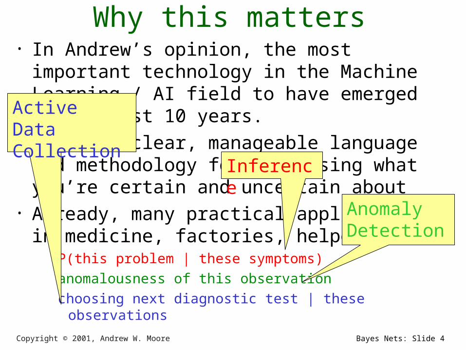
Why this matters• In Andrew’s opinion, the most important
technology in the Machine Learning / AI field to have emerged in the last 10 years.
• A clean, clear, manageable language and methodology for expressing what you’re certain and uncertain about
• Already, many practical applications in medicine, factories, helpdesks:
P(this problem | these symptoms)
anomalousness of this observation
choosing next diagnostic test | these observations
Anomaly Detection
Inference
Active Data Collection
Copyright © 2001, Andrew W. Moore Bayes Nets: Slide 5
Ways to deal with Uncertainty• Three-valued logic: True / False / Maybe• Fuzzy logic (truth values between 0 and 1)• Non-monotonic reasoning (especially
focused on Penguin informatics)• Dempster-Shafer theory (and an extension
known as quasi-Bayesian theory)• Possibabilistic Logic• Probability

Copyright © 2001, Andrew W. Moore Bayes Nets: Slide 6
Discrete Random Variables• A is a Boolean-valued random variable if A
denotes an event, and there is some degree of uncertainty as to whether A occurs.
• Examples• A = The US president in 2023 will be male• A = You wake up tomorrow with a headache• A = You have Ebola

Copyright © 2001, Andrew W. Moore Bayes Nets: Slide 7
Probabilities• We write P(A) as “the fraction of possible
worlds in which A is true”• We could at this point spend 2 hours on the
philosophy of this.• But we won’t.
Copyright © 2001, Andrew W. Moore Bayes Nets: Slide 8
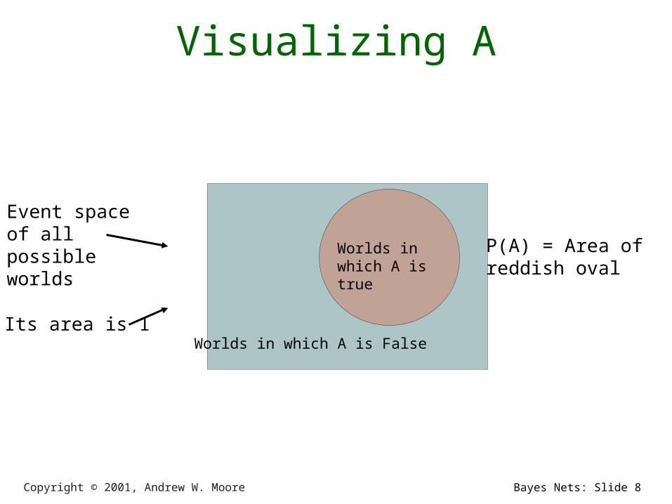
Visualizing A
Event space of all possible worlds
Its area is 1Worlds in which A is False
Worlds in which A is true
P(A) = Area ofreddish oval
Copyright © 2001, Andrew W. Moore Bayes Nets: Slide 9
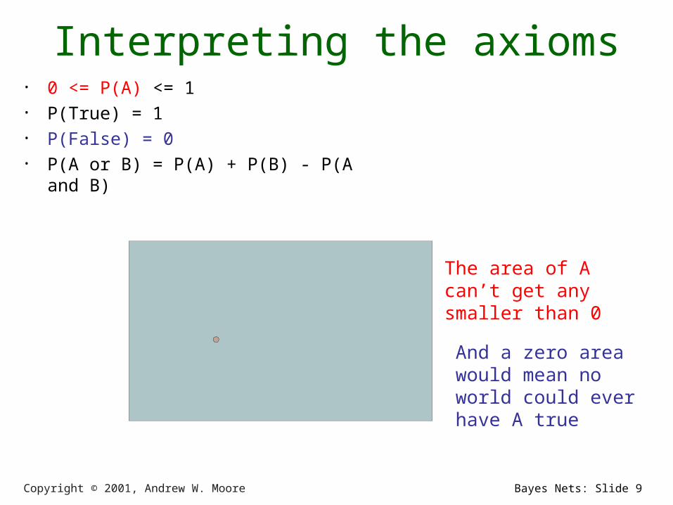
Interpreting the axioms• 0 <= P(A) <= 1• P(True) = 1• P(False) = 0• P(A or B) = P(A) + P(B) - P(A and B)
The area of A can’t get any smaller than 0
And a zero area would mean no world could ever have A true
Copyright © 2001, Andrew W. Moore Bayes Nets: Slide 10
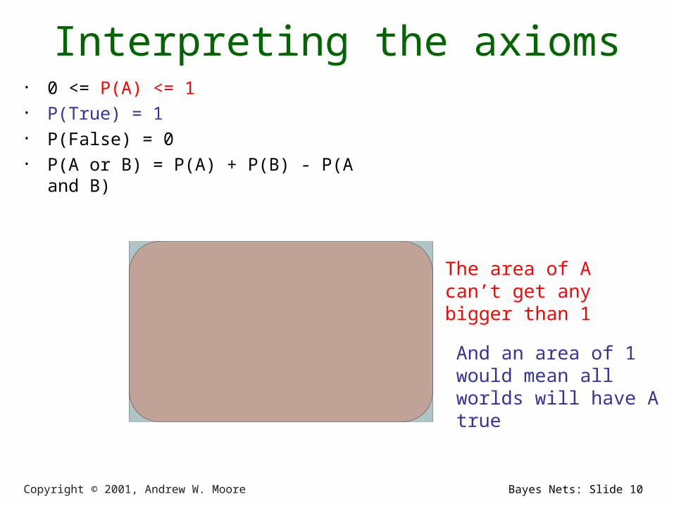
Interpreting the axioms• 0 <= P(A) <= 1• P(True) = 1• P(False) = 0• P(A or B) = P(A) + P(B) - P(A and B)
The area of A can’t get any bigger than 1
And an area of 1 would mean all worlds will have A true

Copyright © 2001, Andrew W. Moore Bayes Nets: Slide 11
Interpreting the axioms• 0 <= P(A) <= 1• P(True) = 1• P(False) = 0• P(A or B) = P(A) + P(B) - P(A and B)
A
B
Copyright © 2001, Andrew W. Moore Bayes Nets: Slide 12
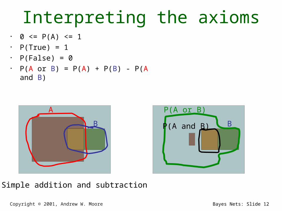
Interpreting the axioms• 0 <= P(A) <= 1• P(True) = 1• P(False) = 0• P(A or B) = P(A) + P(B) - P(A and B)
A
B
P(A or B)
BP(A and B)
Simple addition and subtraction

Copyright © 2001, Andrew W. Moore Bayes Nets: Slide 13
These Axioms are Not to be Trifled With
• There have been attempts to do different methodologies for uncertainty
• Fuzzy Logic• Three-valued logic• Dempster-Shafer• Non-monotonic reasoning
• But the axioms of probability are the only system with this property:
If you gamble using them you can’t be unfairly exploited by an opponent using some other system [di Finetti 1931]
Copyright © 2001, Andrew W. Moore Bayes Nets: Slide 14
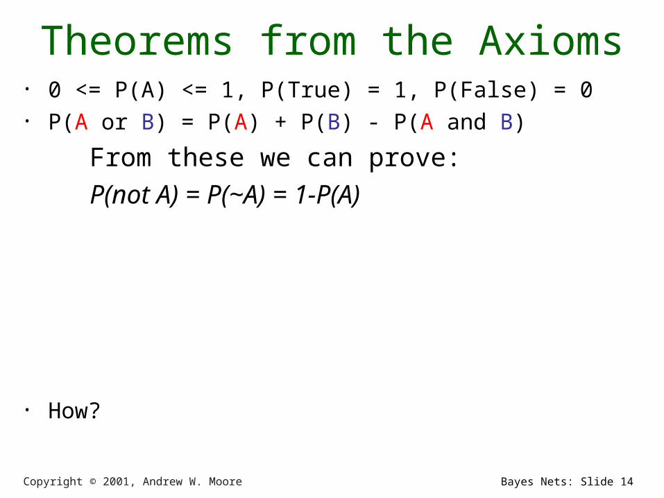
Theorems from the Axioms• 0 <= P(A) <= 1, P(True) = 1, P(False) = 0• P(A or B) = P(A) + P(B) - P(A and B)
From these we can prove:
P(not A) = P(~A) = 1-P(A)
• How?

Copyright © 2001, Andrew W. Moore Bayes Nets: Slide 15
Side Note• I am inflicting these proofs on you for two
reasons:1. These kind of manipulations will need to be
second nature to you if you use probabilistic analytics in depth
2. Suffering is good for you

Copyright © 2001, Andrew W. Moore Bayes Nets: Slide 16
Another important theorem• 0 <= P(A) <= 1, P(True) = 1, P(False) = 0• P(A or B) = P(A) + P(B) - P(A and B)
From these we can prove:
P(A) = P(A ^ B) + P(A ^ ~B)
• How?

Copyright © 2001, Andrew W. Moore Bayes Nets: Slide 17
Conditional Probability• P(A|B) = Fraction of worlds in which B is true
that also have A true
F
H
H = “Have a headache”F = “Coming down with Flu”
P(H) = 1/10P(F) = 1/40P(H|F) = 1/2
“Headaches are rare and flu is rarer, but if you’re coming down with ‘flu there’s a 50-50 chance you’ll have a headache.”

Copyright © 2001, Andrew W. Moore Bayes Nets: Slide 18
Conditional Probability
F
H
H = “Have a headache”F = “Coming down with Flu”
P(H) = 1/10P(F) = 1/40P(H|F) = 1/2
P(H|F) = Fraction of flu-inflicted worlds in which you have a headache
= #worlds with flu and headache ------------------------------------ #worlds with flu
= Area of “H and F” region ------------------------------ Area of “F” region
= P(H ^ F) ----------- P(F)

Copyright © 2001, Andrew W. Moore Bayes Nets: Slide 19
Definition of Conditional Probability
P(A ^ B) P(A|B) = ----------- P(B)
Corollary: The Chain Rule
P(A ^ B) = P(A|B) P(B)
Copyright © 2001, Andrew W. Moore Bayes Nets: Slide 20
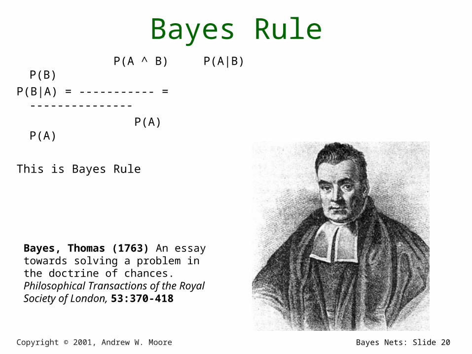
Bayes Rule P(A ^ B) P(A|B) P(B)
P(B|A) = ----------- = ---------------
P(A) P(A)
This is Bayes Rule
Bayes, Thomas (1763) An essay towards solving a problem in the doctrine of chances. Philosophical Transactions of the Royal Society of London, 53:370-418
Copyright © 2001, Andrew W. Moore Bayes Nets: Slide 21
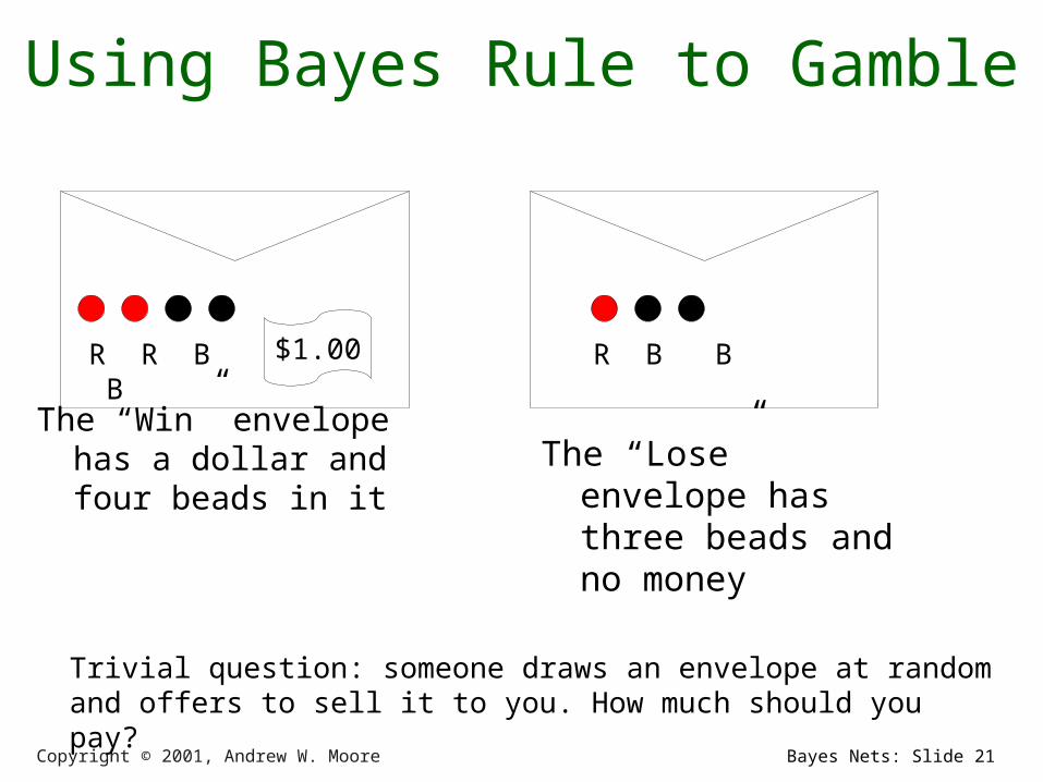
Using Bayes Rule to Gamble
The “Win” envelope has a dollar and four beads in it
$1.00
The “Lose” envelope has three beads and no money
Trivial question: someone draws an envelope at random and offers to sell it to you. How much should you pay?
R R B B R B B

Copyright © 2001, Andrew W. Moore Bayes Nets: Slide 22
Using Bayes Rule to Gamble
The “Win” envelope has a dollar and four beads in it
$1.00
The “Lose” envelope has three beads and no money
Interesting question: before deciding, you are allowed to see one bead drawn from the envelope.
Suppose it’s black: How much should you pay? Suppose it’s red: How much should you pay?

Copyright © 2001, Andrew W. Moore Bayes Nets: Slide 23
Calculation…
$1.00

Copyright © 2001, Andrew W. Moore Bayes Nets: Slide 24
Multivalued Random Variables• Suppose A can take on more than 2 values• A is a random variable with arity k if it can take on
exactly one value out of {v1,v2, .. vk}
• Thus…
jivAvAP ji if 0)(
1)( 21 kvAvAvAP

Copyright © 2001, Andrew W. Moore Bayes Nets: Slide 25
An easy fact about Multivalued Random Variables:• Using the axioms of probability…
0 <= P(A) <= 1, P(True) = 1, P(False) = 0
P(A or B) = P(A) + P(B) - P(A and B)• And assuming that A obeys…
• It’s easy to prove that
jivAvAP ji if 0)(1)( 21 kvAvAvAP
)()(1
21
i
jji vAPvAvAvAP

Copyright © 2001, Andrew W. Moore Bayes Nets: Slide 26
An easy fact about Multivalued Random Variables:• Using the axioms of probability…
0 <= P(A) <= 1, P(True) = 1, P(False) = 0
P(A or B) = P(A) + P(B) - P(A and B)• And assuming that A obeys…
• It’s easy to prove that
jivAvAP ji if 0)(1)( 21 kvAvAvAP
)()(1
21
i
jji vAPvAvAvAP
• And thus we can prove
1)(1
k
jjvAP
Copyright © 2001, Andrew W. Moore Bayes Nets: Slide 27
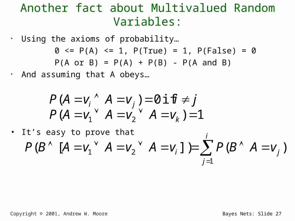
Another fact about Multivalued Random Variables:• Using the axioms of probability…
0 <= P(A) <= 1, P(True) = 1, P(False) = 0
P(A or B) = P(A) + P(B) - P(A and B)• And assuming that A obeys…
• It’s easy to prove that
jivAvAP ji if 0)(1)( 21 kvAvAvAP
)(])[(1
21
i
jji vABPvAvAvABP
Copyright © 2001, Andrew W. Moore Bayes Nets: Slide 28
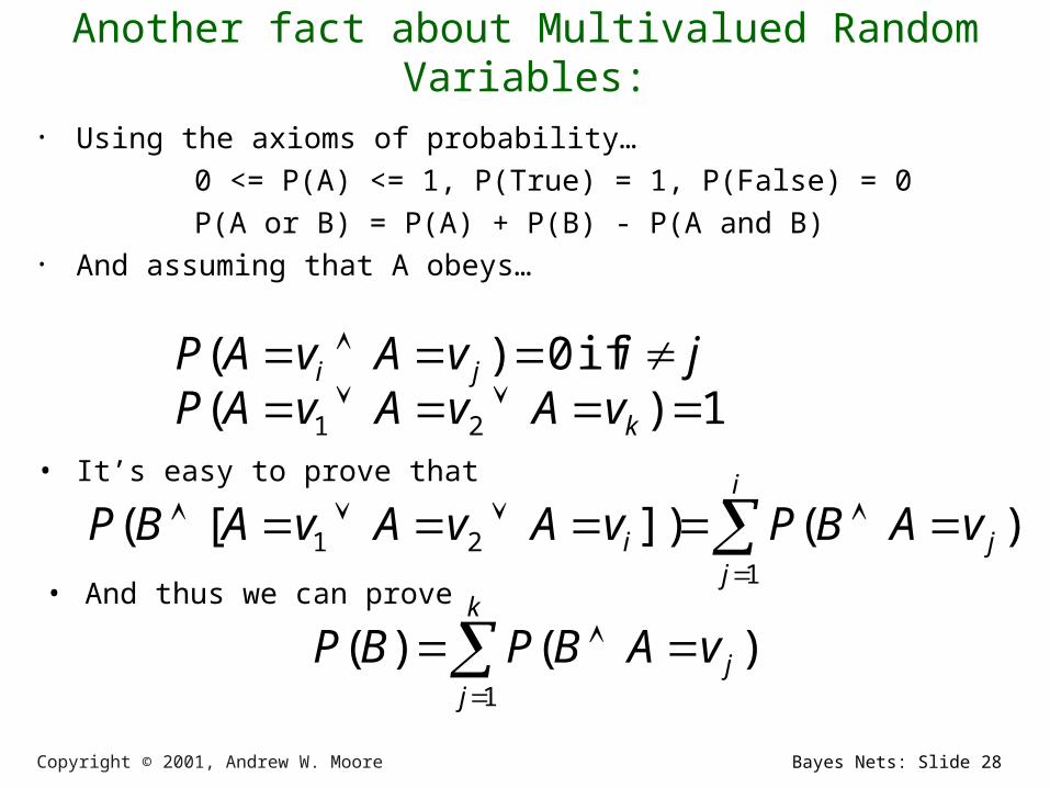
Another fact about Multivalued Random Variables:• Using the axioms of probability…
0 <= P(A) <= 1, P(True) = 1, P(False) = 0
P(A or B) = P(A) + P(B) - P(A and B)• And assuming that A obeys…
• It’s easy to prove that
jivAvAP ji if 0)(1)( 21 kvAvAvAP
)(])[(1
21
i
jji vABPvAvAvABP
• And thus we can prove
)()(1
k
jjvABPBP

Copyright © 2001, Andrew W. Moore Bayes Nets: Slide 29
More General Forms of Bayes Rule
)(~)|~()()|(
)()|()|(
APABPAPABP
APABPBAP
)(
)()|()|(
XBP
XAPXABPXBAP

Copyright © 2001, Andrew W. Moore Bayes Nets: Slide 30
More General Forms of Bayes Rule
An
kkk
iii
vAPvABP
vAPvABPBvAP
1
)()|(
)()|()|(
Copyright © 2001, Andrew W. Moore Bayes Nets: Slide 31
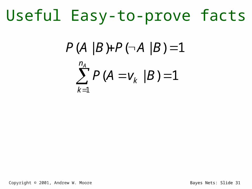
Useful Easy-to-prove facts
1)|()|( BAPBAP
1)|(1
An
kk BvAP
Copyright © 2001, Andrew W. Moore Bayes Nets: Slide 32
The Joint Distribution
Recipe for making a joint distribution of M variables:
Example: Boolean variables A, B, C
Copyright © 2001, Andrew W. Moore Bayes Nets: Slide 33
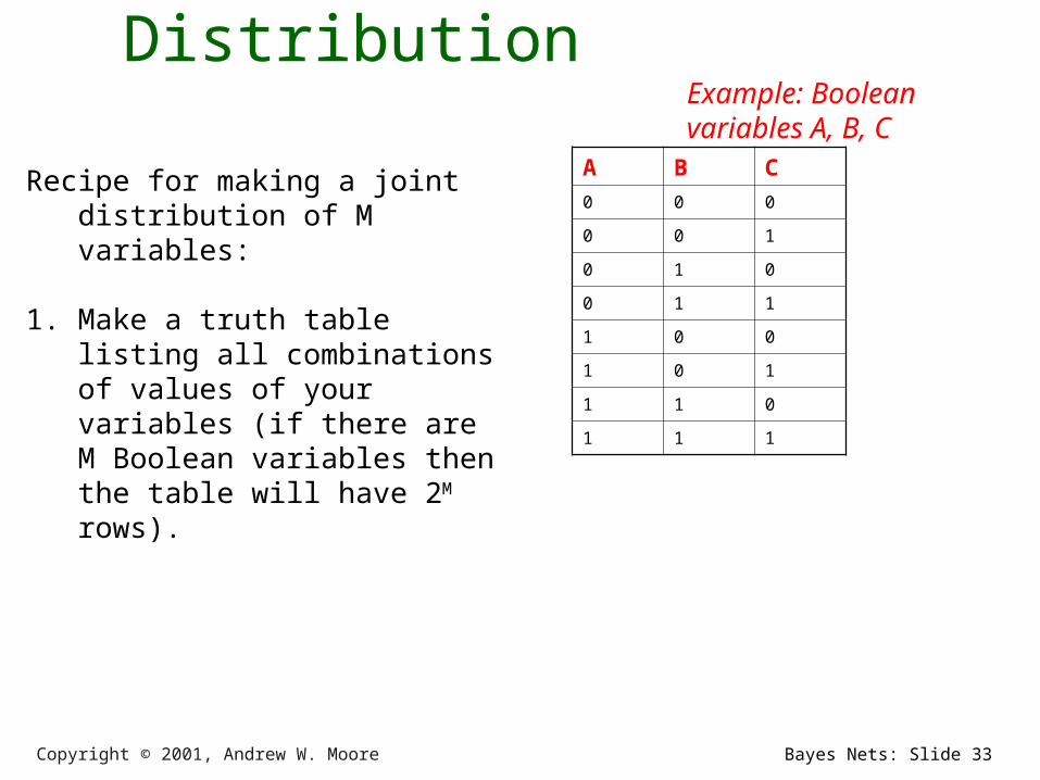
The Joint Distribution
Recipe for making a joint distribution of M variables:
1. Make a truth table listing all combinations of values of your variables (if there are M Boolean variables then the table will have 2M rows).
Example: Boolean variables A, B, C
A B C
0 0 0
0 0 1
0 1 0
0 1 1
1 0 0
1 0 1
1 1 0
1 1 1
Copyright © 2001, Andrew W. Moore Bayes Nets: Slide 34
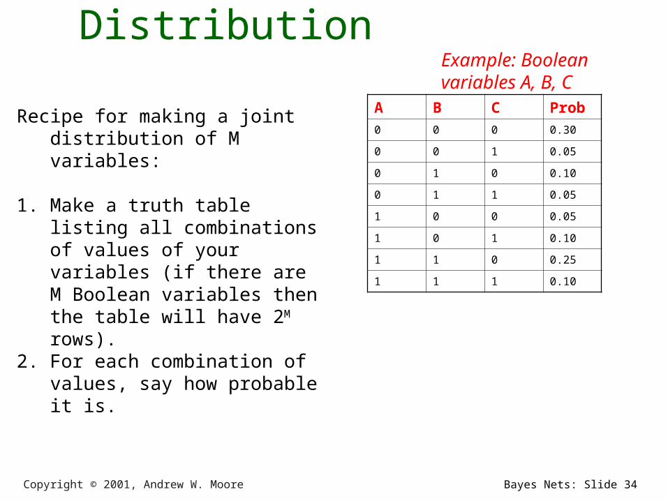
The Joint Distribution
Recipe for making a joint distribution of M variables:
1. Make a truth table listing all combinations of values of your variables (if there are M Boolean variables then the table will have 2M rows).
2. For each combination of values, say how probable it is.
Example: Boolean variables A, B, C
A B C Prob
0 0 0 0.30
0 0 1 0.05
0 1 0 0.10
0 1 1 0.05
1 0 0 0.05
1 0 1 0.10
1 1 0 0.25
1 1 1 0.10

Copyright © 2001, Andrew W. Moore Bayes Nets: Slide 35
The Joint Distribution
Recipe for making a joint distribution of M variables:
1. Make a truth table listing all combinations of values of your variables (if there are M Boolean variables then the table will have 2M rows).
2. For each combination of values, say how probable it is.
3. If you subscribe to the axioms of probability, those numbers must sum to 1.
Example: Boolean variables A, B, C
A B C Prob
0 0 0 0.30
0 0 1 0.05
0 1 0 0.10
0 1 1 0.05
1 0 0 0.05
1 0 1 0.10
1 1 0 0.25
1 1 1 0.10
A
B
C0.050.25
0.10 0.050.05
0.10
0.100.30

Copyright © 2001, Andrew W. Moore Bayes Nets: Slide 36
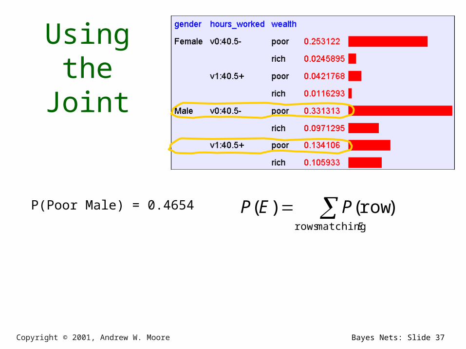
Using the Joint
Once you have the JD you can ask for the probability of any logical expression involving your attribute
E
PEP matching rows
)row()(
Copyright © 2001, Andrew W. Moore Bayes Nets: Slide 37
Using the Joint
P(Poor Male) = 0.4654 E
PEP matching rows
)row()(
Copyright © 2001, Andrew W. Moore Bayes Nets: Slide 38
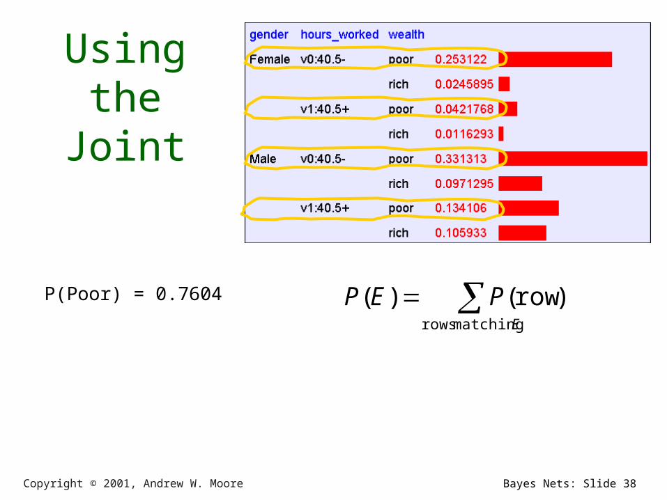
Using the Joint
P(Poor) = 0.7604 E
PEP matching rows
)row()(

Copyright © 2001, Andrew W. Moore Bayes Nets: Slide 39
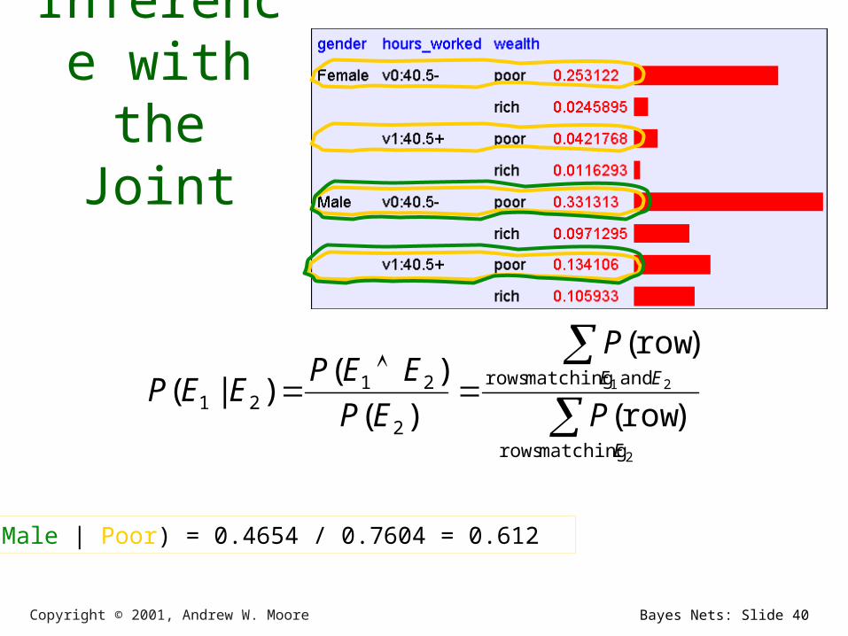
Inference with the
Joint
2
2 1
matching rows
and matching rows
2
2121 )row(
)row(
)(
)()|(
E
EE
P
P
EP
EEPEEP
Copyright © 2001, Andrew W. Moore Bayes Nets: Slide 40
Inference with the
Joint
2
2 1
matching rows
and matching rows
2
2121 )row(
)row(
)(
)()|(
E
EE
P
P
EP
EEPEEP
P(Male | Poor) = 0.4654 / 0.7604 = 0.612

Copyright © 2001, Andrew W. Moore Bayes Nets: Slide 41
Joint distributions• Good news
Once you have a joint distribution, you can ask important questions about stuff that involves a lot of uncertainty
• Bad news
Impossible to create for more than about ten attributes because there are so many numbers needed when you build the damn thing.
Copyright © 2001, Andrew W. Moore Bayes Nets: Slide 42
Using fewer numbersSuppose there are two events:
• M: Manuela teaches the class (otherwise it’s Andrew)• S: It is sunny
The joint p.d.f. for these events contain four entries.
If we want to build the joint p.d.f. we’ll have to invent those four numbers. OR WILL WE??• We don’t have to specify with bottom level conjunctive
events such as P(~M^S) IF…• …instead it may sometimes be more convenient for us
to specify things like: P(M), P(S).But just P(M) and P(S) don’t derive the joint distribution. So
you can’t answer all questions.

Copyright © 2001, Andrew W. Moore Bayes Nets: Slide 43
Using fewer numbersSuppose there are two events:
• M: Manuela teaches the class (otherwise it’s Andrew)• S: It is sunny
The joint p.d.f. for these events contain four entries.
If we want to build the joint p.d.f. we’ll have to invent those four numbers. OR WILL WE??• We don’t have to specify with bottom level conjunctive
events such as P(~M^S) IF…• …instead it may sometimes be more convenient for us
to specify things like: P(M), P(S).But just P(M) and P(S) don’t derive the joint distribution. So
you can’t answer all questions.
What extra assumption can you
make?
Copyright © 2001, Andrew W. Moore Bayes Nets: Slide 44
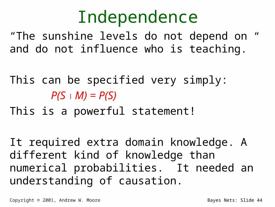
Independence“The sunshine levels do not depend on and do not influence who is teaching.”
This can be specified very simply:
P(S M) = P(S)
This is a powerful statement!
It required extra domain knowledge. A different kind of knowledge than numerical probabilities. It needed an understanding of causation.

Copyright © 2001, Andrew W. Moore Bayes Nets: Slide 45
IndependenceFrom P(S M) = P(S), the rules of probability imply: (can you prove these?)
• P(~S M) = P(~S)
• P(M S) = P(M)
• P(M ^ S) = P(M) P(S)
• P(~M ^ S) = P(~M) P(S), (PM^~S) = P(M)P(~S),
P(~M^~S) = P(~M)P(~S)

Copyright © 2001, Andrew W. Moore Bayes Nets: Slide 46
IndependenceFrom P(S M) = P(S), the rules of probability imply: (can you prove these?)
• P(~S M) = P(~S)
• P(M S) = P(M)
• P(M ^ S) = P(M) P(S)
• P(~M ^ S) = P(~M) P(S), (PM^~S) = P(M)P(~S),
P(~M^~S) = P(~M)P(~S)
And in general:
P(M=u ^ S=v) = P(M=u) P(S=v)
for each of the four combinations of
u=True/False
v=True/False
Copyright © 2001, Andrew W. Moore Bayes Nets: Slide 47
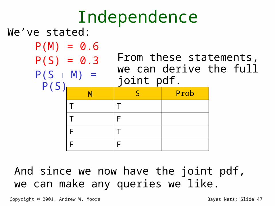
IndependenceWe’ve stated:
P(M) = 0.6P(S) = 0.3P(S M) = P(S)
M S Prob
T T
T F
F T
F F
And since we now have the joint pdf, we can make any queries we like.
From these statements, we can derive the full joint pdf.

Copyright © 2001, Andrew W. Moore Bayes Nets: Slide 48
A more interesting case• M : Manuela teaches the class• S : It is sunny• L : The lecturer arrives slightly late.
Assume both lecturers are sometimes delayed by bad weather. Andrew is more likely to arrive late than Manuela.
Copyright © 2001, Andrew W. Moore Bayes Nets: Slide 49
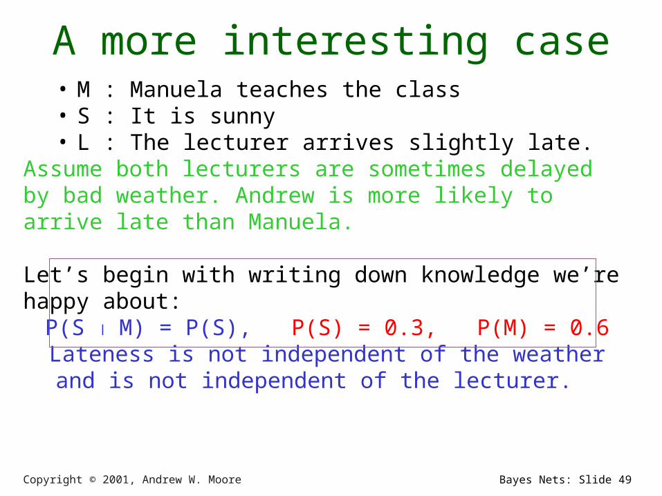
A more interesting case• M : Manuela teaches the class• S : It is sunny• L : The lecturer arrives slightly late.
Assume both lecturers are sometimes delayed by bad weather. Andrew is more likely to arrive late than Manuela.
Let’s begin with writing down knowledge we’re happy about:P(S M) = P(S), P(S) = 0.3, P(M) = 0.6
Lateness is not independent of the weather and is not independent of the lecturer.

Copyright © 2001, Andrew W. Moore Bayes Nets: Slide 50
A more interesting case• M : Manuela teaches the class• S : It is sunny• L : The lecturer arrives slightly late.
Assume both lecturers are sometimes delayed by bad weather. Andrew is more likely to arrive late than Manuela.
Let’s begin with writing down knowledge we’re happy about:P(S M) = P(S), P(S) = 0.3, P(M) = 0.6
Lateness is not independent of the weather and is not independent of the lecturer.
We already know the Joint of S and M, so all we need now isP(L S=u, M=v)
in the 4 cases of u/v = True/False.
Copyright © 2001, Andrew W. Moore Bayes Nets: Slide 51
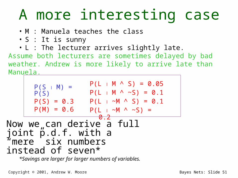
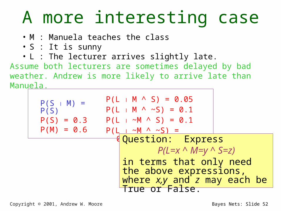
A more interesting case• M : Manuela teaches the class• S : It is sunny• L : The lecturer arrives slightly late.
Assume both lecturers are sometimes delayed by bad weather. Andrew is more likely to arrive late than Manuela.
P(S M) = P(S)P(S) = 0.3P(M) = 0.6
P(L M ^ S) = 0.05P(L M ^ ~S) = 0.1P(L ~M ^ S) = 0.1P(L ~M ^ ~S) = 0.2
Now we can derive a full joint p.d.f. with a “mere” six numbers instead of seven*
*Savings are larger for larger numbers of variables.
Copyright © 2001, Andrew W. Moore Bayes Nets: Slide 52
A more interesting case• M : Manuela teaches the class• S : It is sunny• L : The lecturer arrives slightly late.
Assume both lecturers are sometimes delayed by bad weather. Andrew is more likely to arrive late than Manuela.
P(S M) = P(S)P(S) = 0.3P(M) = 0.6
P(L M ^ S) = 0.05P(L M ^ ~S) = 0.1P(L ~M ^ S) = 0.1P(L ~M ^ ~S) = 0.2
Question: ExpressP(L=x ^ M=y ^ S=z)
in terms that only need the above expressions, where x,y and z may each be True or False.

Copyright © 2001, Andrew W. Moore Bayes Nets: Slide 53
A bit of notationP(S M) = P(S)P(S) = 0.3P(M) = 0.6
P(L M ^ S) = 0.05P(L M ^ ~S) = 0.1P(L ~M ^ S) = 0.1P(L ~M ^ ~S) = 0.2
S M
L
P(s)=0.3P(M)=0.6
P(LM^S)=0.05P(LM^~S)=0.1P(L~M^S)=0.1P(L~M^~S)=0.2

Copyright © 2001, Andrew W. Moore Bayes Nets: Slide 54
A bit of notationP(S M) = P(S)P(S) = 0.3P(M) = 0.6
P(L M ^ S) = 0.05P(L M ^ ~S) = 0.1P(L ~M ^ S) = 0.1P(L ~M ^ ~S) = 0.2
S M
L
P(s)=0.3P(M)=0.6
P(LM^S)=0.05P(LM^~S)=0.1P(L~M^S)=0.1P(L~M^~S)=0.2
Read the absence of an arrow between S and M to mean “it
would not help me predict M if I knew the value of S”
Read the two arrows into L to mean that if I want to know the
value of L it may help me to know M and to know S.
Th
is kind o
f stuff w
ill be
tho
rou
ghly form
alize
d la
ter

Copyright © 2001, Andrew W. Moore Bayes Nets: Slide 55
An even cuter trickSuppose we have these three events:• M : Lecture taught by Manuela• L : Lecturer arrives late• R : Lecture concerns robotsSuppose:• Andrew has a higher chance of being late than Manuela.• Andrew has a higher chance of giving robotics lectures.What kind of independence can we find?
How about:• P(L M) = P(L) ?• P(R M) = P(R) ?• P(L R) = P(L) ?
Copyright © 2001, Andrew W. Moore Bayes Nets: Slide 56
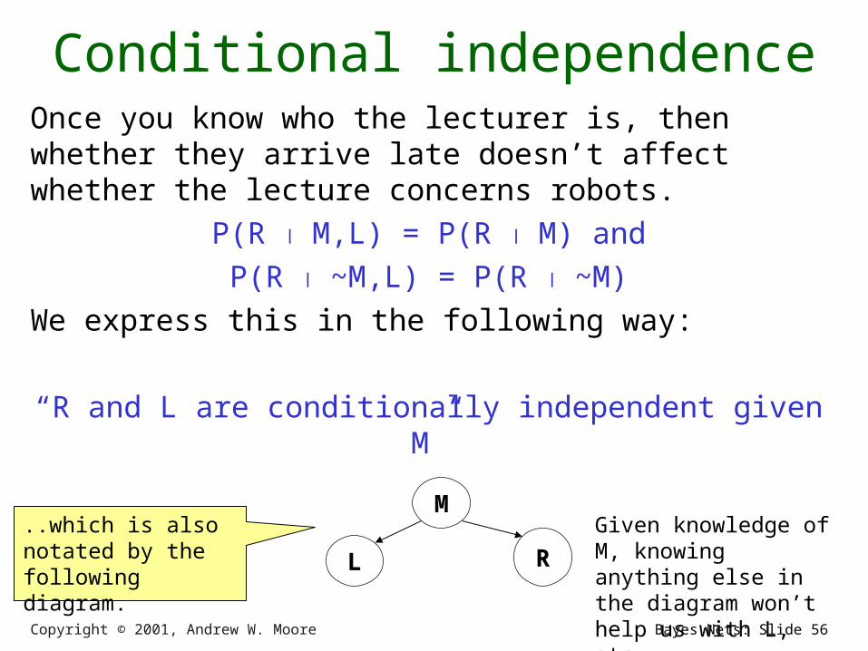
Conditional independenceOnce you know who the lecturer is, then whether they arrive late doesn’t affect whether the lecture concerns robots.
P(R M,L) = P(R M) and
P(R ~M,L) = P(R ~M)
We express this in the following way:
“R and L are conditionally independent given M”
M
L R
Given knowledge of M, knowing anything else in the diagram won’t help us with L, etc.
..which is also notated by the following diagram.

Copyright © 2001, Andrew W. Moore Bayes Nets: Slide 57
Conditional Independence formalizedR and L are conditionally independent given M if
for all x,y,z in {T,F}:
P(R=x M=y ^ L=z) = P(R=x M=y)
More generally:
Let S1 and S2 and S3 be sets of variables.
Set-of-variables S1 and set-of-variables S2 are conditionally independent given S3 if for all assignments of values to the variables in the sets,
P(S1’s assignments S2’s assignments & S3’s assignments)=
P(S1’s assignments S3’s assignments)
Copyright © 2001, Andrew W. Moore Bayes Nets: Slide 58
Example:
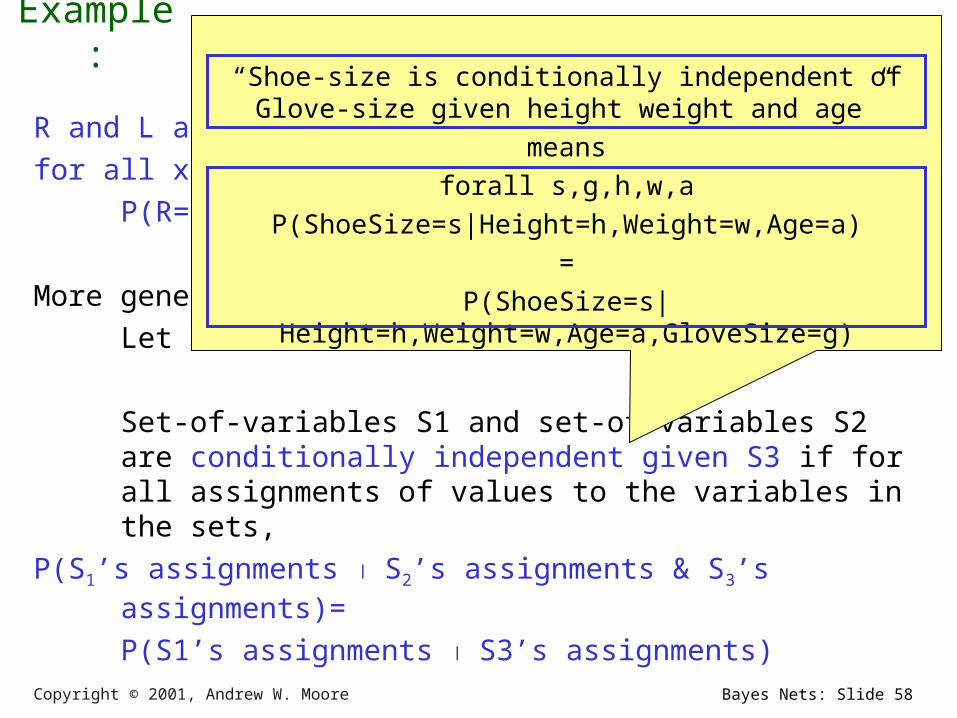
R and L are conditionally independent given M if
for all x,y,z in {T,F}:
P(R=x M=y ^ L=z) = P(R=x M=y)
More generally:
Let S1 and S2 and S3 be sets of variables.
Set-of-variables S1 and set-of-variables S2 are conditionally independent given S3 if for all assignments of values to the variables in the sets,
P(S1’s assignments S2’s assignments & S3’s assignments)=
P(S1’s assignments S3’s assignments)
“Shoe-size is conditionally independent of Glove-size given height weight and age”
means
forall s,g,h,w,a
P(ShoeSize=s|Height=h,Weight=w,Age=a)
=
P(ShoeSize=s|Height=h,Weight=w,Age=a,GloveSize=g)

Copyright © 2001, Andrew W. Moore Bayes Nets: Slide 59
Example:
R and L are conditionally independent given M if
for all x,y,z in {T,F}:
P(R=x M=y ^ L=z) = P(R=x M=y)
More generally:
Let S1 and S2 and S3 be sets of variables.
Set-of-variables S1 and set-of-variables S2 are conditionally independent given S3 if for all assignments of values to the variables in the sets,
P(S1’s assignments S2’s assignments & S3’s assignments)=
P(S1’s assignments S3’s assignments)
“Shoe-size is conditionally independent of Glove-size given height weight and age”
does not mean
forall s,g,h
P(ShoeSize=s|Height=h)
=
P(ShoeSize=s|Height=h, GloveSize=g)

Copyright © 2001, Andrew W. Moore Bayes Nets: Slide 60
Conditional independence
M
L R
We can write down P(M). And then, since we know L is only directly influenced by M, we can write down the values of P(LM) and P(L~M) and know we’ve fully specified L’s behavior. Ditto for R.
P(M) = 0.6 P(L M) = 0.085 P(L ~M) = 0.17 P(R M) = 0.3 P(R ~M) = 0.6
‘R and L conditionally independent given M’

Copyright © 2001, Andrew W. Moore Bayes Nets: Slide 61
Conditional independenceM
L R
P(M) = 0.6
P(L M) = 0.085
P(L ~M) = 0.17
P(R M) = 0.3
P(R ~M) = 0.6
Conditional Independence:
P(RM,L) = P(RM),
P(R~M,L) = P(R~M)
Again, we can obtain any member of the Joint prob dist that we desire:
P(L=x ^ R=y ^ M=z) =
Copyright © 2001, Andrew W. Moore Bayes Nets: Slide 62
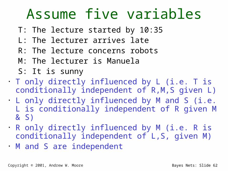
Assume five variablesT: The lecture started by 10:35L: The lecturer arrives lateR: The lecture concerns robotsM: The lecturer is ManuelaS: It is sunny
• T only directly influenced by L (i.e. T is conditionally independent of R,M,S given L)
• L only directly influenced by M and S (i.e. L is conditionally independent of R given M & S)
• R only directly influenced by M (i.e. R is conditionally independent of L,S, given M)
• M and S are independent

Copyright © 2001, Andrew W. Moore Bayes Nets: Slide 63
Making a Bayes net
S M
R
L
T
Step One: add variables.• Just choose the variables you’d like to be included in the
net.
T: The lecture started by 10:35L: The lecturer arrives lateR: The lecture concerns robotsM: The lecturer is ManuelaS: It is sunny

Copyright © 2001, Andrew W. Moore Bayes Nets: Slide 64
Making a Bayes net
S M
R
L
T
Step Two: add links.• The link structure must be acyclic.• If node X is given parents Q1,Q2,..Qn you are promising
that any variable that’s a non-descendent of X is conditionally independent of X given {Q1,Q2,..Qn}
T: The lecture started by 10:35L: The lecturer arrives lateR: The lecture concerns robotsM: The lecturer is ManuelaS: It is sunny

Copyright © 2001, Andrew W. Moore Bayes Nets: Slide 65
Making a Bayes net
S M
R
L
T
P(s)=0.3P(M)=0.6
P(RM)=0.3P(R~M)=0.6
P(TL)=0.3P(T~L)=0.8
P(LM^S)=0.05P(LM^~S)=0.1P(L~M^S)=0.1P(L~M^~S)=0.2
Step Three: add a probability table for each node.• The table for node X must list P(X|Parent Values) for each
possible combination of parent values
T: The lecture started by 10:35L: The lecturer arrives lateR: The lecture concerns robotsM: The lecturer is ManuelaS: It is sunny

Copyright © 2001, Andrew W. Moore Bayes Nets: Slide 66
Making a Bayes net
S M
R
L
T
P(s)=0.3P(M)=0.6
P(RM)=0.3P(R~M)=0.6
P(TL)=0.3P(T~L)=0.8
P(LM^S)=0.05P(LM^~S)=0.1P(L~M^S)=0.1P(L~M^~S)=0.2
• Two unconnected variables may still be correlated• Each node is conditionally independent of all non-
descendants in the tree, given its parents.• You can deduce many other conditional independence
relations from a Bayes net. See the next lecture.
T: The lecture started by 10:35L: The lecturer arrives lateR: The lecture concerns robotsM: The lecturer is ManuelaS: It is sunny

Copyright © 2001, Andrew W. Moore Bayes Nets: Slide 67
Bayes Nets FormalizedA Bayes net (also called a belief network) is an augmented directed acyclic graph, represented by the pair V , E where:
• V is a set of vertices.• E is a set of directed edges joining vertices. No
loops of any length are allowed.
Each vertex in V contains the following information:• The name of a random variable• A probability distribution table indicating how the
probability of this variable’s values depends on all possible combinations of parental values.

Copyright © 2001, Andrew W. Moore Bayes Nets: Slide 68
Building a Bayes Net1. Choose a set of relevant variables.2. Choose an ordering for them
3. Assume they’re called X1 .. Xm (where X1 is the first in the ordering, X1 is the second, etc)
4. For i = 1 to m:
1. Add the Xi node to the network
2. Set Parents(Xi ) to be a minimal subset of {X1…Xi-1} such that we have conditional independence of Xi and all other members of {X1…Xi-1} given Parents(Xi )
3. Define the probability table of
P(Xi =k Assignments of Parents(Xi ) ).

Copyright © 2001, Andrew W. Moore Bayes Nets: Slide 69
Example Bayes Net BuildingSuppose we’re building a nuclear power station.There are the following random variables:
GRL : Gauge Reads Low.CTL : Core temperature is low.FG : Gauge is faulty.FA : Alarm is faultyAS : Alarm sounds
• If alarm working properly, the alarm is meant to sound if the gauge stops reading a low temp.
• If gauge working properly, the gauge is meant to read the temp of the core.

Copyright © 2001, Andrew W. Moore Bayes Nets: Slide 70
Computing a Joint EntryHow to compute an entry in a joint distribution?
E.G: What is P(S ^ ~M ^ L ~R ^ T)?
S M
RL
T
P(s)=0.3P(M)=0.6
P(RM)=0.3P(R~M)=0.6
P(TL)=0.3P(T~L)=0.8
P(LM^S)=0.05P(LM^~S)=0.1P(L~M^S)=0.1P(L~M^~S)=0.2

Copyright © 2001, Andrew W. Moore Bayes Nets: Slide 71
Computing with Bayes Net
P(T ^ ~R ^ L ^ ~M ^ S) =P(T ~R ^ L ^ ~M ^ S) * P(~R ^ L ^ ~M ^ S) = P(T L) * P(~R ^ L ^ ~M ^ S) =P(T L) * P(~R L ^ ~M ^ S) * P(L^~M^S) =P(T L) * P(~R ~M) * P(L^~M^S) =P(T L) * P(~R ~M) * P(L~M^S)*P(~M^S) =P(T L) * P(~R ~M) * P(L~M^S)*P(~M | S)*P(S) =P(T L) * P(~R ~M) * P(L~M^S)*P(~M)*P(S).
S M
RL
T
P(s)=0.3P(M)=0.6
P(RM)=0.3P(R~M)=0.6
P(TL)=0.3P(T~L)=0.8
P(LM^S)=0.05P(LM^~S)=0.1P(L~M^S)=0.1P(L~M^~S)=0.2
Copyright © 2001, Andrew W. Moore Bayes Nets: Slide 72
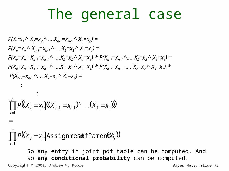
The general case
P(X1=x1 ^ X2=x2 ^ ….Xn-1=xn-1 ^ Xn=xn) =
P(Xn=xn ^ Xn-1=xn-1 ^ ….X2=x2 ^ X1=x1) =
P(Xn=xn Xn-1=xn-1 ^ ….X2=x2 ^ X1=x1) * P(Xn-1=xn-1 ^…. X2=x2 ^ X1=x1) =
P(Xn=xn Xn-1=xn-1 ^ ….X2=x2 ^ X1=x1) * P(Xn-1=xn-1 …. X2=x2 ^ X1=x1) *
P(Xn-2=xn-2 ^…. X2=x2 ^ X1=x1) =
:
:
=
n
iiii
n
iiiii
XxXP
xXxXxXP
1
11111
Parents of sAssignment
So any entry in joint pdf table can be computed. And so any conditional probability can be computed.

Copyright © 2001, Andrew W. Moore Bayes Nets: Slide 73
Where are we now?• We have a methodology for building Bayes nets.
• We don’t require exponential storage to hold our probability table. Only exponential in the maximum number of parents of any node.
• We can compute probabilities of any given assignment of truth values to the variables. And we can do it in time linear with the number of nodes.
• So we can also compute answers to any questions.
E.G. What could we do to compute P(R T,~S)?
S M
RL
T
P(s)=0.3P(M)=0.6
P(RM)=0.3P(R~M)=0.6
P(TL)=0.3P(T~L)=0.8
P(LM^S)=0.05P(LM^~S)=0.1P(L~M^S)=0.1P(L~M^~S)=0.2

Copyright © 2001, Andrew W. Moore Bayes Nets: Slide 74
Where are we now?• We have a methodology for building Bayes nets.
• We don’t require exponential storage to hold our probability table. Only exponential in the maximum number of parents of any node.
• We can compute probabilities of any given assignment of truth values to the variables. And we can do it in time linear with the number of nodes.
• So we can also compute answers to any questions.
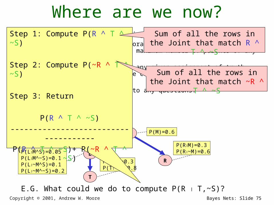
E.G. What could we do to compute P(R T,~S)?
S M
RL
T
P(s)=0.3P(M)=0.6
P(RM)=0.3P(R~M)=0.6
P(TL)=0.3P(T~L)=0.8
P(LM^S)=0.05P(LM^~S)=0.1P(L~M^S)=0.1P(L~M^~S)=0.2
Step 1: Compute P(R ^ T ^ ~S)
Step 2: Compute P(~R ^ T ^ ~S)
Step 3: Return
P(R ^ T ^ ~S)
-------------------------------------
P(R ^ T ^ ~S)+ P(~R ^ T ^ ~S)
Copyright © 2001, Andrew W. Moore Bayes Nets: Slide 75
Where are we now?• We have a methodology for building Bayes nets.
• We don’t require exponential storage to hold our probability table. Only exponential in the maximum number of parents of any node.
• We can compute probabilities of any given assignment of truth values to the variables. And we can do it in time linear with the number of nodes.
• So we can also compute answers to any questions.
E.G. What could we do to compute P(R T,~S)?
S M
RL
T
P(s)=0.3P(M)=0.6
P(RM)=0.3P(R~M)=0.6
P(TL)=0.3P(T~L)=0.8
P(LM^S)=0.05P(LM^~S)=0.1P(L~M^S)=0.1P(L~M^~S)=0.2
Step 1: Compute P(R ^ T ^ ~S)
Step 2: Compute P(~R ^ T ^ ~S)
Step 3: Return
P(R ^ T ^ ~S)
-------------------------------------
P(R ^ T ^ ~S)+ P(~R ^ T ^ ~S)
Sum of all the rows in the Joint that match R ^ T ^ ~S
Sum of all the rows in the Joint that match ~R ^ T ^ ~S

Copyright © 2001, Andrew W. Moore Bayes Nets: Slide 76
Where are we now?• We have a methodology for building Bayes nets.
• We don’t require exponential storage to hold our probability table. Only exponential in the maximum number of parents of any node.
• We can compute probabilities of any given assignment of truth values to the variables. And we can do it in time linear with the number of nodes.
• So we can also compute answers to any questions.
E.G. What could we do to compute P(R T,~S)?
S M
RL
T
P(s)=0.3P(M)=0.6
P(RM)=0.3P(R~M)=0.6
P(TL)=0.3P(T~L)=0.8
P(LM^S)=0.05P(LM^~S)=0.1P(L~M^S)=0.1P(L~M^~S)=0.2
Step 1: Compute P(R ^ T ^ ~S)
Step 2: Compute P(~R ^ T ^ ~S)
Step 3: Return
P(R ^ T ^ ~S)
-------------------------------------
P(R ^ T ^ ~S)+ P(~R ^ T ^ ~S)
Sum of all the rows in the Joint that match R ^ T ^ ~S
Sum of all the rows in the Joint that match ~R ^ T ^ ~S
Each of these obtained by the “computing a joint probability entry” method of the earlier slides
4 joint computes
4 joint computes

Copyright © 2001, Andrew W. Moore Bayes Nets: Slide 77
The good news
We can do inference. We can compute any conditional probability:
P( Some variable Some other variable values )
2
2 1
matching entriesjoint
and matching entriesjoint
2
2121 )entryjoint (
)entryjoint (
)(
)()|(
E
EE
P
P
EP
EEPEEP

Copyright © 2001, Andrew W. Moore Bayes Nets: Slide 78
The good news
We can do inference. We can compute any conditional probability:
P( Some variable Some other variable values )
2
2 1
matching entriesjoint
and matching entriesjoint
2
2121 )entryjoint (
)entryjoint (
)(
)()|(
E
EE
P
P
EP
EEPEEP
Suppose you have m binary-valued variables in your Bayes Net and expression E2 mentions k variables.
How much work is the above computation?
Copyright © 2001, Andrew W. Moore Bayes Nets: Slide 79
The sad, bad newsConditional probabilities by enumerating all matching entries
in the joint are expensive:
Exponential in the number of variables.
Copyright © 2001, Andrew W. Moore Bayes Nets: Slide 80
The sad, bad newsConditional probabilities by enumerating all matching entries
in the joint are expensive:
Exponential in the number of variables.
But perhaps there are faster ways of querying Bayes nets?• In fact, if I ever ask you to manually do a Bayes Net
inference, you’ll find there are often many tricks to save you time.
• So we’ve just got to program our computer to do those tricks too, right?

Copyright © 2001, Andrew W. Moore Bayes Nets: Slide 81
The sad, bad newsConditional probabilities by enumerating all matching entries
in the joint are expensive:
Exponential in the number of variables.
But perhaps there are faster ways of querying Bayes nets?• In fact, if I ever ask you to manually do a Bayes Net
inference, you’ll find there are often many tricks to save you time.
• So we’ve just got to program our computer to do those tricks too, right?
Sadder and worse news:General querying of Bayes nets is NP-complete.

Copyright © 2001, Andrew W. Moore Bayes Nets: Slide 82
Bayes nets inference algorithmsA poly-tree is a directed acyclic graph in which no two nodes have more than one path between them.
A poly tree Not a poly tree(but still a legal Bayes net)
S
RL
T
L
T
MSM
R
X1X2
X4X3
X5
X1 X2
X3
X5
X4
• If net is a poly-tree, there is a linear-time algorithm (see a later Andrew lecture).
• The best general-case algorithms convert a general net to a poly-tree (often at huge expense) and calls the poly-tree algorithm.
• Another popular, practical approach (doesn’t assume poly-tree): Stochastic Simulation.

Copyright © 2001, Andrew W. Moore Bayes Nets: Slide 83
Sampling from the Joint Distribution
It’s pretty easy to generate a set of variable-assignments at random with the same probability as the underlying joint distribution.
How?
S M
RL
T
P(s)=0.3P(M)=0.6
P(RM)=0.3P(R~M)=0.6
P(TL)=0.3P(T~L)=0.8
P(LM^S)=0.05P(LM^~S)=0.1P(L~M^S)=0.1P(L~M^~S)=0.2

Copyright © 2001, Andrew W. Moore Bayes Nets: Slide 84
Sampling from the Joint Distribution
1. Randomly choose S. S = True with prob 0.32. Randomly choose M. M = True with prob 0.63. Randomly choose L. The probability that L is true
depends on the assignments of S and M. E.G. if steps 1 and 2 had produced S=True, M=False, then probability that L is true is 0.1
4. Randomly choose R. Probability depends on M.5. Randomly choose T. Probability depends on L
S M
RL
T
P(s)=0.3P(M)=0.6
P(RM)=0.3P(R~M)=0.6
P(TL)=0.3P(T~L)=0.8
P(LM^S)=0.05P(LM^~S)=0.1P(L~M^S)=0.1P(L~M^~S)=0.2
Copyright © 2001, Andrew W. Moore Bayes Nets: Slide 85
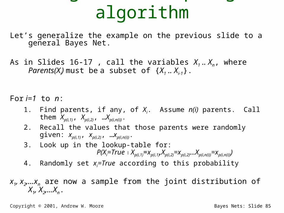
A general sampling algorithmLet’s generalize the example on the previous slide to a general Bayes Net.
As in Slides 16-17 , call the variables X1 .. Xn, where Parents(Xi) must be a subset of {X1 .. Xi-1}.
For i=1 to n:
1. Find parents, if any, of Xi. Assume n(i) parents. Call them Xp(i,1), Xp(i,2), …Xp(i,n(i)).
2. Recall the values that those parents were randomly given: xp(i,1), xp(i,2), …xp(i,n(i)).
3. Look up in the lookup-table for: P(Xi=True Xp(i,1)=xp(i,1),Xp(i,2)=xp(i,2)…Xp(i,n(i))=xp(i,n(i)))
4. Randomly set xi=True according to this probability
x1, x2,…xn are now a sample from the joint distribution of X1, X2,…Xn.

Copyright © 2001, Andrew W. Moore Bayes Nets: Slide 86
Stochastic Simulation ExampleSomeone wants to know P(R = True T = True ^ S = False )
We’ll do lots of random samplings and count the number of occurrences of the following:
• Nc : Num. samples in which T=True and S=False.
• Ns : Num. samples in which R=True, T=True and S=False.
• N : Number of random samplings
Now if N is big enough:
Nc /N is a good estimate of P(T=True and S=False).
Ns /N is a good estimate of P(R=True ,T=True , S=False).
P(RT^~S) = P(R^T^~S)/P(T^~S), so Ns / Nc can be a good estimate of P(RT^~S).
Copyright © 2001, Andrew W. Moore Bayes Nets: Slide 87
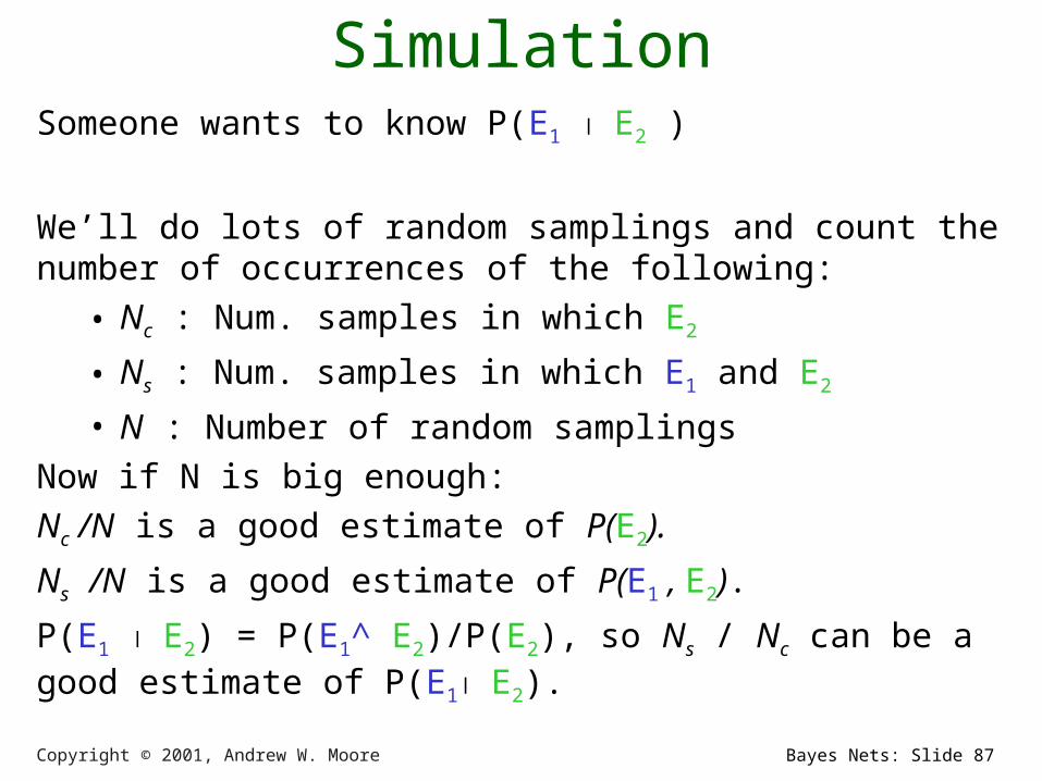
General Stochastic SimulationSomeone wants to know P(E1 E2 )
We’ll do lots of random samplings and count the number of occurrences of the following:
• Nc : Num. samples in which E2
• Ns : Num. samples in which E1 and E2
• N : Number of random samplings
Now if N is big enough:
Nc /N is a good estimate of P(E2).
Ns /N is a good estimate of P(E1 , E2).
P(E1 E2) = P(E1^ E2)/P(E2), so Ns / Nc can be a good estimate of P(E1 E2).
Copyright © 2001, Andrew W. Moore Bayes Nets: Slide 88
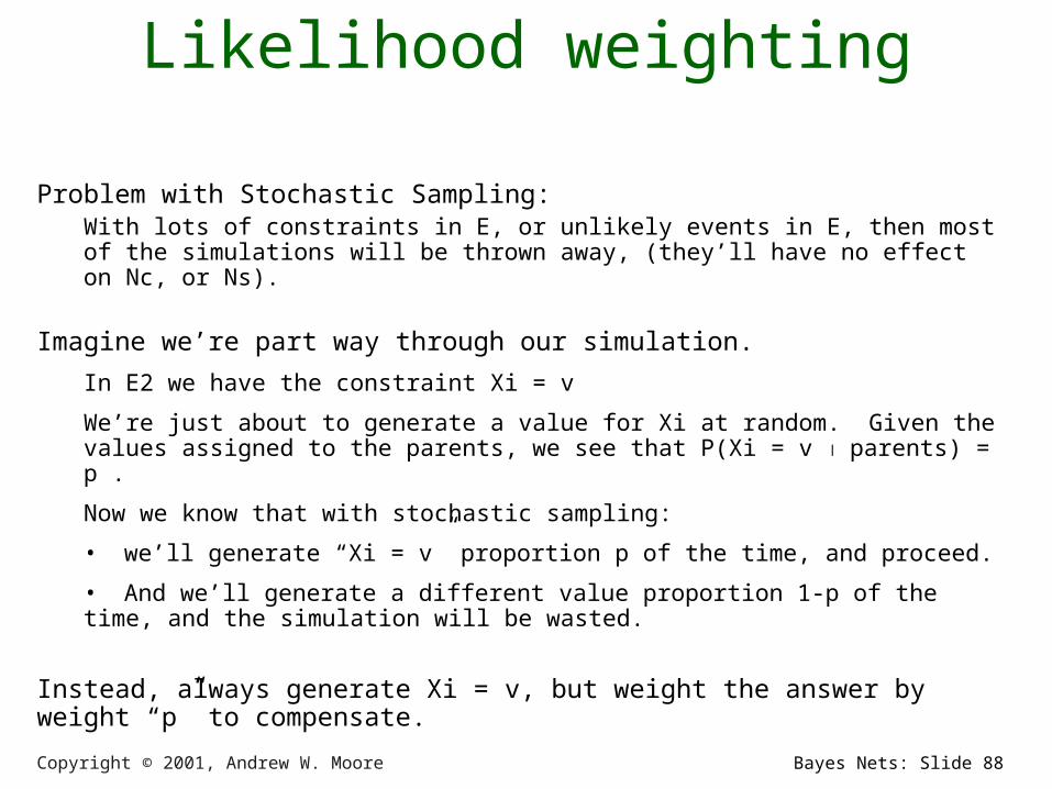
Likelihood weighting
Problem with Stochastic Sampling:With lots of constraints in E, or unlikely events in E, then most of the simulations will be thrown away, (they’ll have no effect on Nc, or Ns).
Imagine we’re part way through our simulation.
In E2 we have the constraint Xi = v
We’re just about to generate a value for Xi at random. Given the values assigned to the parents, we see that P(Xi = v parents) = p .
Now we know that with stochastic sampling:
• we’ll generate “Xi = v” proportion p of the time, and proceed.
• And we’ll generate a different value proportion 1-p of the time, and the simulation will be wasted.
Instead, always generate Xi = v, but weight the answer by weight “p” to compensate.

Copyright © 2001, Andrew W. Moore Bayes Nets: Slide 89
Likelihood weightingSet Nc :=0, Ns :=0
1. Generate a random assignment of all variables that matches E2. This process returns a weight w.
2. Define w to be the probability that this assignment would have been generated instead of an unmatching assignment during its generation in the original algorithm.Fact: w is a product of all likelihood factors involved in the generation.
3. Nc := Nc + w
4. If our sample matches E1 then Ns := Ns + w
5. Go to 1
Again, Ns / Nc estimates P(E1 E2 )
Copyright © 2001, Andrew W. Moore Bayes Nets: Slide 90
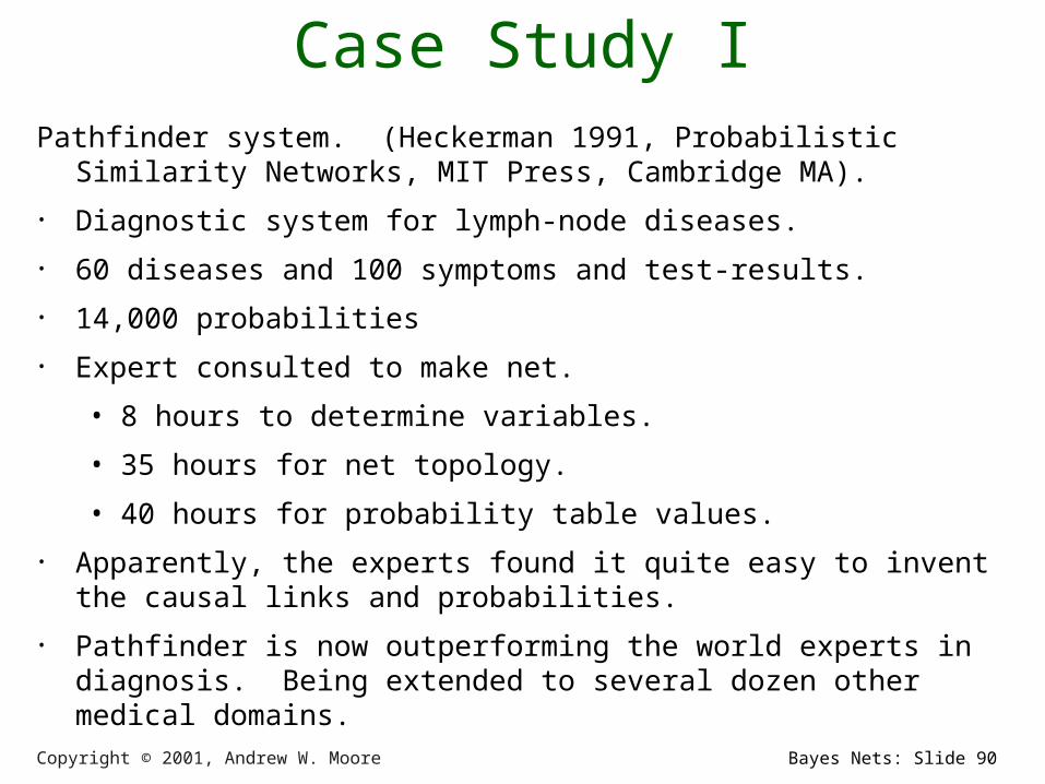
Case Study IPathfinder system. (Heckerman 1991, Probabilistic Similarity Networks,
MIT Press, Cambridge MA).
• Diagnostic system for lymph-node diseases.
• 60 diseases and 100 symptoms and test-results.
• 14,000 probabilities
• Expert consulted to make net.
• 8 hours to determine variables.
• 35 hours for net topology.
• 40 hours for probability table values.
• Apparently, the experts found it quite easy to invent the causal links and probabilities.
• Pathfinder is now outperforming the world experts in diagnosis. Being extended to several dozen other medical domains.

Copyright © 2001, Andrew W. Moore Bayes Nets: Slide 91
Questions• What are the strengths of probabilistic networks
compared with propositional logic?• What are the weaknesses of probabilistic networks
compared with propositional logic?• What are the strengths of probabilistic networks
compared with predicate logic?• What are the weaknesses of probabilistic networks
compared with predicate logic?• (How) could predicate logic and probabilistic
networks be combined?
Copyright © 2001, Andrew W. Moore Bayes Nets: Slide 92
What you should know• The meanings and importance of independence
and conditional independence.• The definition of a Bayes net.• Computing probabilities of assignments of
variables (i.e. members of the joint p.d.f.) with a Bayes net.
• The slow (exponential) method for computing arbitrary, conditional probabilities.
• The stochastic simulation method and likelihood weighting.