4 Classical Dynamics

4.1 Newtonian gravity

4.1.1 Basic law of attraction

Two point masses, with mass M1 and M2, lying at r1 and r2, attract one

another. M1 feels a force from M2

F 12 = force on M1 from M2 = GM1M2

r312r12

where r12 = r1 r2 = vector from 2 to 1 and r12 = jr12j

CoordinateOrigin

M1

r

r1F12

F21

M2

2

SimilarlyM2 feels a force from M1

F 21 = force on M2 from M1 = GM2M1

r321r21 = +

GM1M2

r312r12 = F 12

where r21 = r2r1 is the vector from 1 to 2. We have used r21 = r12, and

jr21j = jr12j. Thus, the gravitational forces are equal and opposite. This is in

accordance with Newton's 3rd law and ensures that the composite system of

(M1+M2) does not suddenly start moving as a whole and violating Newton's

1st law.

Notice also that the gravitational force at M1 fromM2 is directed exactly

at M2. It is a \central" force: F 12 is parallel to r12. This remark causes us

to digress and mention: : :

60

4.1.2 The little known codicil to Newton's 3rd law

Many books, e.g. Marion, state Newton's laws in something like this form:

1. A body remains at rest or in uniform motion unless acted upon by a

force.

2. A body acted upon by a force moves in such a manner that the time

rate of change of momentum equals the force.

3. If two bodies exert forces on each other, these forces are equal in mag-

nitude and opposite in direction.

This statement of 3 is WRONG! The correct statement is

30. If two bodies exert forces on each other, these forces are equal in mag-

nitude and opposite in direction AND ALONG THE SAME LINE.

Newton knew this, but modern text book writers have garbled it.

A

B B

ANOT OK!

(b)(a)

OK

If (b) were possible, then we could take the two particles A and B, nail

one to the hub of a wheel, the other to the center, and watch as the wheel

accelerated up to innite angular velocity.

61

Thus, while one often hears about the \central force" nature of gravita-

tion, this is actually a property of any action-at-a-distance, classical force

law.

You might wonder about the magnetic force between two moving par-

ticles in electromagnetism. This does not seem to be a central force. The

explanation is that the electromagnetic eld itself carries momentum and

angular momentum. Classical electromagnetism cannot be written as a pure

action-at-a-distance theory. That is, there is more to Maxwell's equations

than just the Coulomb law.

4.1.3 Gravitational Potential

The force onM1, due toM2's presence can be written in terms of the gradient

of a gravitational potential:

F 12 = force at M1 due to M2

= force at position r1 due to mas at r2

= M1

@

@x1

GM2

jr1 r2j

!;@

@y1

GM2

jr1 r2j

!;@

@z1

GM2

jr1 r2j

!!

= M1r1V (r1)

where r1 is the gradient operator at M1;

@@x1; @@y1; @@z1

. V (r) is the gravi-

tational potential at r1,

V = GM2

jr1 r2j:

The potential at point r from a number of masses; at r1; r2; r3; : : : ; rn is, in

general

V = NXi=1

GMi

jr rijwhere the sum excludes any mass exactly at r (do not include the innite

self-energy!).

62

4.2 The 2-body problem

Although every mass in the universe exerts a force on every other mass,

there is a useful idealization where the mutual interaction of just two masses

dominates their motion. The equations of motion are then

M1r1 = GM1M2

jr1 r2j3(r1 r2)

M2r2 = GM1M2

jr1 r2j3(r2 r1) :

These apply, for example, to binary stars at large separations, but small

enough that the tidal eects of other stars in the galaxy can be neglected.

Or, the orbit of the Earth around the Sun, to the extent that the eects of

the Moon and other planets can be ignored.

4.2.1 Conservation laws for 2-body orbits

For a 2-body system, we want to solve for 6 functions of time r1(t) and r2(t),

and 12 constants will appear in the solution (equivalent to 2 vectors of initial

positions and 2 vectors of initial velocities). It is most ecient to approach

this problem by nding constants of the motion (to reduce the number of

equations to solve) and by choosing a convenient set of coordinates in which

to work.

Add the two equations of motion given above. Then, since the forces are

equal and opposite, the right hand side sums to zero, and we are left with

M1r1 +M2r2 = 0 :

Let the center of mass of the system be at R; then by the denition of center

of mass as the mass-weighted average position,

R =M1r1 +M2r2

(M1 +M2)

63

we get

(M1 +M2) R = 0 or R = 0 :

Thus, the location of the center of mass of the system is unaccelerated, since

there is no external force on the system.

It follows that the center of mass moves at a constant velocity:

_R dR

dt= v = constant

R = R0 + v0t :

This relation expresses the \Conservation of Linear Momentum." R0 and

V 0 are the rst 6 \constants of motion."

The next logical thing to do is to change to center-of-mass coordinates

r01; r

02, that is, to coordinates relative to the center of mass.

CoM

M2

M1

2r

1r

1r ′

2r ′

R

O

The relevant relationships are:

r1 = R+ r01

r2 = R+ r02

R = R0 + v0t :

Substituting these into the equations of motion, we get

M1r01 = GM1M2

jr01 r02j3(r01 r02)

64

M2r02 = GM1M2

jr01 r02j3(r02 r01) :

Note that the equations preserve exactly the form they had before: We could

have just written down the answer without calculation. We can arbitrarily

choose coordinates relative to the CoM, because the CoM frame is a good

inertial frame. Any change of origin (R0) and/or change of velocity (V 0) is

allowed by (so-called) \Gallilean invariance."

So let us choose to do this: coordinates are, henceforth, measured relative

to the CoM; and we drop the primes.

In CoM system,

M1r1 = GM1M2

jr1 r2j3(r1 r2)

M2r2 = GM1M2

jr1 r2j3(r2 r1)

with M1r1 +M2r2 = 0 by denition.

We can now construct further integrals of the motion. Consider the total

angular momentum about the CoM: L =M1r1 _r1 +M2r2 _r2. Then

dL

dt= M1 (r1 r1 + _r1 _r1) +M2 (r2 r2 + _r2 _r2)

= M1r1 r1 +M2r2 r2 :

Substitute the equations of motion for M1r1 and M2r2, then

dL

dt= GM1M2

jr1 r2j3fr1 (r1 r2) + r2 (r2 r1)g

=GM1M2

jr1 r2j3(r1 r2 + r2 r1)

= 0

i.e. the total angular momentum of the system is conserved:

L = constant.

65

That is, the angular momentum vector is xed in direction and magnitude

(because no external torques are acting).

1rCoM

L

M1

r1

r2 M

2

r2

The angular momentum provides 3 more integrals of the motion, so we are

now up to 9.

We can also look at the total energy of the system:

E = (kinetic energy) + (potential energy)

=

1

2M1 _r1 _r1 +

1

2M2 _r2 _r2

+

GM1M2

jr1 r2j

!:

To see that this is conserved, write

dE

dt=M1 _r1 r1 +M2 _r2 r2 +

GM1M2

jr1 r2j2d

dtjr1 r2j :

Now

d

dtjr1 r2j =

d

dt(r1 r1 + r2 r2 2r1 r2)1=2

=r1 _r1 + r2 _r2 r1 _r2 _r1 r2

jr1 r2j=

(r1 r2)( _r1 _r2)

jr1 r2j:

Therefore

dE

dt= _r1

M1r1 +

GM1M2

jr1 r2j3(r1 r2)

!+ _r2

M2r2 +

GM1M2

jr1 r2j3(r2 r1)

!

= 0

using the equations of motion. Therefore the total energy of the system,

E = constant

66

(because no work is being done on systems by an external force). The energy

is another integral of the motion (each one equivalent in counting to one

initial condition). These 10 integrals, R0;v0;L; E are general to N bodies,

not just 2 (as we will see later). To completely specify the system we need

12 constants of integration; 10 specied: 2 remain. These turn out to be

particular to the special case of 2-bodies. That is, they are more like \initial

conditions" than \conservation laws."

4.2.2 Two-body orbits

Finally we are ready to solve the 2-body problem. Let us recap: We have

removed 6 integrals of the motion by working in the center of mass (= center

of momentum frame). Then the other integrals of the motion are total energy

and total angular momentum.

The positions of the two bodies, r1 and r2, obey

M1r1 =GM1M2

jr1 r2j3(r1 r2) (1)

M2r2 =GM1M2

jr1 r2j3(r2 r1) (2)

and by denition

M1r1 +M2r2 = 0 : (3)

We showed that

M1r1 _r1 +M2r2 _r2 = L L = constant vector

1

2M1 _r1 _r1 +

1

2M2 _r2 _r2

GM1M2

jr1 r2j= E : E = constant scalar

We now want to completely solve the system: for r1(t) and r2(t).

67

It is convenient to reduce the system to simpler form by working in terms

of the separation vector of the two bodies:

r = r1 r2 = vector from body 2 to body 1.

2M1M CoM 2r1r

−1r 2r r=

Then consider equation (1) divided by M1 minus equation (2) divided by

M2:

r = (r1 r2) =G(M1 +M2)

jr1 r2j3(r1 r2)

or

r = GMr3

r

where M = M1 +M2 is the total mass of the system. This equation says

that body 1 moves as if it was of very small mass being attracted by mass

(M1 +M2) at body 2; the separation vector is accelerated by the total mass

of the system. The fact that the 2-body problem reduces to the equation of

the \one-body problem" (test mass in the central force eld of a ctitious

mass M) is an amazing and nonobvious result!

With the relations

r = r1 r2

M1r1 +M2r2 = 0

we can nd how to calculate r1 and r2 from the solutions for r:

r1 =M2

Mr r2 =

M1

Mr :

68

Note that the signs are opposite (the masses must be on opposite sides of

the CoM).

Eliminating r1 and r2 in favor of r we nd that r(t) obeys

r = GMr3

r

r _r =M

M1M2

L

1

2_r _r GM

r=

M

M1M2

E :

Notice the appearance of a quantity M1M2=(M1 +M2) on the right

hand sides, where we expect (one over) a mass. The quantity is called the

reduced mass. Notice that is smaller than both M1 and M2.

The angular momentum equation

r _r =

M

M1M2

L

has an important immediate consequence. Since r (r _r) = _r (r _r) = 0,

that is, the vector cross product of two vectors is perpendicular to both of

them, r and _r are both perpendicular to L, i.e. all the motion occurs in a

plane perpendicular to L (remember that r1 and r2 are proportional to r,

hence parallel to r).

Adopting coordinates in the plane of the orbit, we can write in Cartesian

coordinates:

L = (0; 0; L)

r = (x; y; 0)

_r = ( _x; _y; 0) :

The momentum equation becomes

x _y y _x =

M

M1M2

L =

L

69

with an energy equation

1

2( _x2 + _y2) GM

(x2 + y2)1=2=

M

M1M2

E =

E

:

In principle the above two equations are the coupled dierential equations

for the two unknowns x(t) and y(t). It is simpler, however, to exploit the

planar geometry in polar coordinates r and .

+ dt)r (t

δθθ^

azimuthal angle direction

0

δθr

r (t)

rδ δr

particle trajectory

radial direction

r

If r(t)! r(t+ dt) in time dt, then, to rst order,

(component of r along original radial direction) = r

(component of r along direction of azimuth) = r :

Therefore if, at any given time, in cylindrical coordinates (r; ; z),

r = (r; 0; 0) rer

_r =r(t+ t) r(t)

t=

r

t; r

t; 0

!= _rer + r _e

r _r =0; 0; r2 _

_r _r = _r2 + r2 _2

70

.er θθ

.r

er r.

\Centrifugal form of Pythagoras"

We nd that the angular momentum equation is

r2 _ =

M

M1M2

L =

L

while the energy equation is

1

2

_r2 + r2 _2

GM

r=

M

M1M2

E =

E

:

The angular momentum equation can be interpreted geometrically

r(t)t

t + dt

r(t + dt) dA

d (t)θ

In interval t to t+ dt, the vector between the objects sweeps at area dA,

dA =1

2r rd :

Therefore, the rate of change of area is

dA

dt=

1

2r2 _

which by the rst equation becomes

dA

dt=

1

2

M

M1M2

L =

L

2= constant.

71

Thus, it is a simple consequence of the Law of momentum conservation that

the rate of sweeping out of area is a constant.

This is Kepler's Second Law (1609). Kepler discovered it empirically |

he had no idea what physics was behind it. Kepler was Tycho's \graduate

student" (in modern terms), but Tycho would never let him look at all the

data. Tycho died in 1601, and Kepler got the data then. Even today many

observers would rather take their data to the grave than let theorists analyze

them. (Or so it seems to theorists!)

Proceeding, we can get one equation for r(t) by eliminating _ from these

equations. Then the equations can be rewritten

dr

dt

!2

= 2M

M1M2

E +2GM

r

M

M1M2

2 L2

r2 d

dt

!=

M

M1M2

L

r2:

4.2.3 Shapes of the orbits

The above equations could be solved for r(t) and (t). The answer comes

out in \elliptic integral functions." But the shape of the orbit can be derived

by eliminating time from the equations to get an equation for r():

dr

d=

r2

(L=)

"2(E=) +

2(GM)

r (L=)2

r2

#1=2

where we are now using the \reduced mass"

M1M2=M :

This is a rst order dierential equation that can be integrated

Z r (L=) dr

r2h2(E=) + 2(GM)

r (L=)2

r2

i1=2 =Z

d = 0

72

where 0 = constant of integration. Dene a constant

r0 =(L=)2

(GM)=

L2

GM2

which sets a scale for the orbit, and a second constant,

2 = 1 +2(E=)(L=)2

(GM)2= 1 +

2EL2

(GM)23:

Then the integral can be rewritten

Z r r0dr

r22

1 r0

r

21=2 = ( 0)

which, via the substitution

cos u = 1 r0

r

becomes (try it!)

Z u

du = ( 0) ) u = ( 0) ) 1

r=

1

r0(1 cos( 0))

the plus-or-minus is thrown in gratuitously, because it corresponds to 0, an

unknown constant, changing by ; so we can write the result with the more

convenient + sign,

1

r=

1

r0(1 + cos( 0)) :

This is the equation of a conic section.

There are three special cases which we now consider.

Case of < 1:

If < 1, then 1r> 0 for all ; so the separation between the two masses

remains nite: the objects remain bound with

r0

1 + r r0

1 :

73

The orbit in this case, is an ellipse. If we put

x = r cos( 0)

y = r sin( 0)

and eliminate and r, the equation of the orbit becomes

1

(x2 + y2)1=2=

1

r0

1 +

x

(x2 + y2)1=2

!

which simplies to x+ a

a

2+y2

b2= 1

where

a =r0

1 2; b =

r0

(1 2)1=2

are semi-major and semi-minor axes.

x = a(1 − ), y = 0b r

ax

y

0

θ0θ + π/2

εa

=

r = r /(1 + ε), θ = θ 0

ε

r = r /(1 − ε), θ = θ + π0 0

x = − a(1 + ε), y = 0

The axial ratio of the ellipse is b=a = (1 2)1=2. The quantitiy r0 is called

the \semi-latus rectum." Note that < 1 implies, from the denition

2 1 +2EL2

(GM)23

that E < 0, i.e. the total energy of a bound system is negative.

74

We can also see that the orbit is periodic and closed. Let us nd the

period:

1

r=

1

r0(1 + cos( 0))

d

dt=

(L=)

r2

are the equations governing (t); we can write this as a single equation for

(t);

r20(L=)

Z d

(1 + cos( 0))2=Z t

dt :

Now, in one repeating orbit,

increases from ! + 2

t increases from t ! t+ ; ; = period, so

r20(L=)

Z 2

0

d

(1 + cos )2= :

The substitution t = tan 12 (so d = 2dt

1+t2; cos = 1t2

1+t2) renders this integral

tractable. Then

=r20

(L=) 2

(1 2)3=2

Eliminating r0 and in terms of physical variables: (L=) = (GMr0)1=2 and

r0 = a(1 2), a the semi-major axis,

= 2a3=2

(GM)1=2:

Note, incidentally (you can check) that a depends only on the total energy

a = GM1M2=(2E), while depends on both the energy and the angular

momentum. For bound orbits we have now proved Kepler's laws:

1. The planets move in ellipses with the sun (the center of mass) at one

focus:

1

r=

1

r0(1 + cos( 0))

75

with < 1 ( = 0 is circle).

2. A line from the Sun to a planet sweeps out equal areas in equal times:

dA

dt=

1

2(L=) :

(Note, this also works for unbound orbits.)

3. The square of the period of revolution is proportional to the cube of

the semi-major axis

2

2=

a3

GMor !2 =

GM

a3:

(Note this involves the total mass M =M1 +M2.)

Case of > 1:

Again from the denition,

= 1 +2EL2

(GM)23

we see that E > 0, so the total energy of system is positive. This will imply

that the orbit is unbound:

1

r=

1

r0(1 + cos( 0))

is a hyperbola: x = r cos( 0), y = r sin( 0) gives, again

1

(x2 + y2)1=2=

1

r0

1 +

x

(x2 + y2)1=2

!

) (x a)2

a2 y2

b2= 1

a =r0

2 1b =

r0

(2 1)1=2

b = a(2 1)1=2

76

y

x

y = 0, x = a(ε − 1)

M2

M1

r0

is at one focus; Hyperbola; single-pass orbit.M0

Case of = 1:

From the denition of , = 1 ) E = 0, i.e. total energy of system is

zero. In this case the orbit is a parabola:

1

r=

1

r0(1 + cos( 0))

) y2 = r20 2r0x

y

x

M2r0

M1 r0/2

Parabola. Single pass orbit.

77

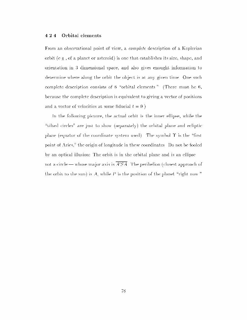
4.2.4 Orbital elements

From an observational point of view, a complete description of a Keplerian

orbit (e.g., of a planet or asteroid) is one that establishes its size, shape, and

orientation in 3 dimensional space, and also gives enought information to

determine where along the orbit the object is at any given time. One such

complete description consists of 6 \orbital elements." (There must be 6,

because the complete description is equivalent to giving a vector of positions

and a vector of velocities at some ducial t = 0.)

In the following picture, the actual orbit is the inner ellipse, while the

\tilted circles" are just to show (separately) the orbital plane and ecliptic

plane (equator of the coordinate system used). The symbol is the \rst

point of Aries," the origin of longitude in these coordinates. Do not be fooled

by an optical illusion: The orbit is in the orbital plane and is an ellipse |

not a circle | whose major axis is A0SA. The perihelion (closest approach of

the orbit to the sun) is A, while P is the position of the planet \right now."

78

The 6 orbital elements are dened as [2 \shape" parameters]:

semimajor axis a half the length of AA0

eccentricity e (1 b2=a2)1=2 if b is the semiminor axis

[2 parameters dene the orbital plane: ]

inclination i angle (6 QNB) between the orbital

plane and the ecliptic plane

longitude of the angle (6 SN) from rst point of Aries

ascending node to the line of nodes N 0N . \Ascending"

means pick the node where the planetcrosses the ecliptic from south (below)to north (above.)

[1 parameter orients the orbit in its plane: ]

argument of perihelion ! angle (6 NSA1) from the ascendingnode, measured in the plane of theorbit, to the perihelion point A.

[1 parameter species orbital phase: ]

time of perihelion passage T one of the precise times that the object

passes through to the point A

Note that P , the period is not an orbital element, since you can compute it

from a by

P (in years) = [a (in AU) ]3=2 :

Instead of !, people sometimes quote the \longitude of perihelion"

$ + ! = 6 SN + 6 NSA1 :

(The symbol $ is actually a weird form of \pi," but most astronomers call it

\pomega"!) Note that the two summed angles are measured along two dier-

79

ent planes! This is not really the longitude of anything, but it approximates

it when the inclination i is small.

Also, instead of T , people sometimes give the \longitude" L of the planet

at a specied epoch (time). Here the longitude is again a kind of phoney:

L 6 N + 6 NP1 :

In case you want to compute locations of the planets, here are the values

of their orbital elements, called \ephimerides" (the plural of \ephemeris"):

Planets: Mean Elements

(For epoch J2000:0 = JD24515450 = 2000 January 1.5)

Planet Inclination (i) Eccentricity (e)

Mercury 700017:0095051 0.2056317524914Venus 323040:0007828 0.0067718819142

Earth 0.0 0.0167086171540Mars 150059:0001532 0.0934006199474Jupiter 118011:0077079 0.0484948512199Saturn 229019:0096115 0.0555086217172Uranus 046023:0050621 0.0462958985125Neptune 146011:0082795 0.0089880948652

Pluto 1708031:008 0.249050

Mean Longitude Mean Longitude Mean Longitude

of Node () of Perihelion ($) of Epoch (L)

Mercury 4819051:0021495 7727022:0002855 25215003:0025985

Venus 7640047:0071268 13133049:0034607 18158047:0028304

Earth 0.0 10256014:0045310 10027059:0021464

Mars 4933029:0013554 33603036:0084233 35525059:0078866Jupiter 10027051:0098631 1419052:0071326 3421005:0034211Saturn 11339055:0088533 9303024:0043421 5004038:0089695

Uranus 7400021:0041002 17300018:0057320 31403018:0001840

Neptune 13147002:0060528 4807025:0028581 30420055:0019574

Pluto 11017049:007 22408005:005 23844038:002

80

Mean Distance (AU) Mean Distance (1011 m)

Mercury 0.3870983098 0.579090830

Venus 0.7233298200 1.08208601

Earth 1.0000010178 1.49598023

Mars 1.5236793419 2.27939186

Jupiter 5.2026031913 7.78298361

Saturn 9.5549095957 14.29394133

Uranus 19.2184460618 28.75038615

Neptune 30.1103868694 45.04449769

Pluto 39.544674 59.157990

4.2.5 The mass of the Sun and the masses of binary stars

We have seen that the sidereal period of a planet, , is related to the semi-

major axis of its orbit, a, by

2 =

42

GM

!a3 ;

where

M =M +mplanet :

This formula has been applied to calculate GM on the last column of the

following table.

Observed Inferred

Sidereal Semi-majorperiod axis of orbit GM

Planet (days) (AU) (1026 cm3 s1)

Mercury 87.969 0.387099 1.32714

Venus 224.701 0.723332 1.32713

Earth 365.256 1.000000 1.32713Mars 686.980 1.523691 1.32712

Jupiter 4332.589 5.202803 1.32839Saturn 10759.22 9.53884 1.32750

Uranus 30685.4 19.1819 1.32715

Neptune 60189 30.0578 1.32723Pluto 90465 39.44 1.32727

81

Therefore, from the low-mass planets,

GM = 1:32713 1026 cm3 s1 :

This is known very accurately, to 1 part in 106. Amazingly, G itself,

from laboratory experiments, is only known to about 1 part in 104 as (6:670

0:004)108 cm3 s1 g1. So our knowledge of the mass of the Sun is limited

by laboratory physics, not astronomical observations!

M = (1:989 0:001) 1033 gm :

We can also estimate the mass of Jupiter, MJ :

G(M +MJ) = 1:32839 1026 cm3 s1

G(M +ME) = 1:32713 1026 cm3 s1 ;

where ME is the mass of the Earth. Jupiter has about an 0.1% eect on

GM . Thus MJ 0:1% of solar mass. Furthermore,

G(MJ ME) = 1:26 1023 cm3 s1

MJ ME

M

= 0:000949 ;

which gives us

MJ 0:000949M ' 1:89 1030 g :

This is fairly inaccurate (1 part in 103), and it is a good illustration of an

important principle: normally, we measure planet masses by their eects on

the satellites or one another. Articial satellites (e.g., Voyager II at Uranus)

are also good!

This works for our Sun, but what about other stars? Their planets are

too faint: there are no low-mass test particles that we can see around these

82

stars. But > 50% of all stars are in multiple star systems. So we can use the

relative motions of binary stars to get stellar masses.

The periods of binary stars vary typically from a few hours (e.g., 6h

for Mirzam, alias Ursa Majoris) to hundreds of years (e.g., 700 yr for 61

Cygni). Some are even shorter, but for these it is likely that the stars are

highly distorted by tidal eects and their masses will be subject to systematic

errors (e.g., \semidetached" or \contact" binaries).

A variety of data may be available for a binary star. We may see the

motion of one star around the other on the sky (which is rare), or we may

see only variations in the velocities of the stars (as seen from Doppler shifts

in their spectra | this is more common). Binary stars may be single-lined

(see light from only one star) or double-lined.

Consider, for example, the second case, a \double-lined spectroscopic

binary star." Here, we see the two stars' spectra superimposed, and we

can measure the radial velocities for both stars, but the stars are too close

together for us to see their orbits by measuring the changing positions of the

stars relative to one another. Then what we see are star velocities like

system velocity not,in general, zero

velo

city

, v

time, t /τ

τ

0 .5 1 1.5

K1

K2

83

Immediately, we see that we have three observables:

the orbital period,

the peak velocity of the less massive star 1, K1 (the more massive star

moves more slowly)

the peak velocity of star 2, K2

The shape of the curves is here sinusoidal, which implies circular orbits,

" = 0. Other shapes are possible for O " 1.

What can we get from these data? To simplify things, suppose the stars

are in a circular orbit, " = 0 (not necessary | we could t " from the velocity

data if we wanted to, but this makes things harder). Then our orbit equations

are

M1r1 +M2r2 = 0 center of mass at rest

d

dt=L=

r20= constant =

2

= constant angular velocity ; circular orbit.

But the period is related to the separation of the stars, r (the same as the

semimajor axis, for a circular orbit), by

2 =42r3

GMfor circular orbits,

and the speeds of the stars in their orbits are v1 = r1 and v2 = r2. If the

orbital plane is parallel to the line of sight, the peak velocities we would see

for the stars are r1 and r2. In general, however, this will not be the case

(see gure on the next page).

At inclination angle i (i = angle between line of sight and normal to

orbital plane)

84

K1 = r1 sin i =2

r1 sin i

K2 = r2 sin i =2

r2 sin i :

If i = 0, we see no velocity. Thus, the separation of the stars is

r = r1 + r2 = (K1 +K2)

2 sin i:

Using the previous formula for 2 and eliminating r, the period equation then

gives a total mass

M1 +M2 =

2G (K1 +K2)

3

sin3 i:

The center of the mass provides the constraint M1r1 = M2r2, so the mass

ratio is

M2

M1

=r1

r2=K1

K2

:

Putting these together,

M1 sin3 i =

1

2G (K1 +K2)

2K2

M2 sin3 i =

1

2G (K1 +K2)

2K1 :

85

Here the right hand sides are completely known, so we infer the left-

hand sides. These data only give masses if we know the inclination of the

orbit, i. But, in general, we will not know this, so our data only measure a

combination of masses and i.

For one special group of stars, we do get M1 and M2 directly | from

\eclipsing" binaries, where the light curve shows an eclipse (see gure).

1.2

1

.8

.6

.4

.2

00 .5 1 1.5

primaryeclipse

secondaryeclipse

τ

time, /τt

light

flu

x, F

/(F 1

+F

)2

Here, the stars are eclipsing one another . This scenario is only possible

if i 90 (provided that the stellar radii separation, which we can check

in the above equations; if this is not true, the stars are so distorted that we

cannot use this method anyway). Thus, sin i 1. Errors in i have little

eect on the masses derived, because sin i changes slowly at i 90.

In fact, the best data on masses of stars comes from eclipsing spectroscopic

double-lined binaries, even though these are hard to nd.

An alternative approach is to measure many noneclipsing binaries, assume

i to be selected at random, and use statistics to derive the distribution of

masses, M1 and M2.

86

4.2.6 Supernovae in binary systems

It is quite common for a supernova to be in a binary system. In fact, some

supernovae are caused by a companion star's dumping mass on a star, until

the latter explodes (section 4.3.4, below). What happens to the binary system

when the explosion occurs? It turns out that the force of the explosion is not

an important eect on the star, but its mass loss is.

Before the supernova we have (say) two stars in circular orbit:

1 2r rM

2

v2M1

v1

CoM

Putting the CoM at rest, we have

M1v1 +M2v2 = 0

M1r1 +M2r2 = 0 :

LetM1 be the mass that explodes. Typically it is the more massive star that

explodes, so M1 > M2. When it explodes, it quickly (and spherically, say)

blows o most of its mass, so that its new mass M 01 is

M 01 =M1 M

and we have

87

M2

v2M1

v1

oldCoM

newCoM

′

expanding shellof masscentered on

M1′

M1

M1−

A rst important eect is that the remaining binary is not at rest. Let's

calculate its new CoM velocity vc:

M 01v1 +M2v2 = (M 0

1 +M2)vc :

Or, using v1 = M2v2=M1 and M01 =M1 M ,

(M1 M)M2

M1

v2

+M2v2 = (M1 M +M2)vc

giving

vc =MM2

M1(M1 +M2 M)v2 :

Notice that as M !M1 (all-star explosion!), vc ! v2, as it must.

Typical values might be M1 = 10M,M2 = 5M, M = 8:5M, leaving

a 1:5M neutron star for M 01, so

vc =8:5 5

10 6:5v2 = 0:65v2 :

88

For close binaries, v2 can be hundreds of kilometers per second, so the system

really takes o!

In fact, we need to check whether the binary remains bound at all! The

easiest way to do this is to see if its total energy in the new CoM is positive

or negative just after the explosion:

E0 =

total energy

in new CoM

!=

0B@

total

kinetic

energy

1CA

0B@

kinetic

energy

of CoM

1CA+

potential

energy

!

=

1

2M 0

1v21 +

1

2M2v

22

1

2(M 0

1 +M2) v2c

GM 01M2

r:

Recall that (Section 4.2.2) the separation vector r and the relative velocity

v2 v1 satisfy Kepler's Laws with the total mass. So for circular orbits,

G(M1 +M2)

r= (v2 v1)2 :

Substituting this, and vc previously obtained, and also eliminating M 01 in

favor of M1 M and v1 in favor of v2M2=M1, we get

E0 =1

2(M1 M)

M2v2

M1

2+1

2M2v

22

1

2(M1 +M2 M)

"

MM2v2

M1(M1 +M2 M)

#2 (M1 M)M2

M1 +M2

1 +

M2

M1

v2

2:

Now a fairly amazing algebraic simplication (I used the \Simplify [ ]"

function in Mathematica on the computer) gives

E0 = 1

2M2v

22

(M1 M)(M1 +M2)

M21 (M1 +M2 M)

(M1 +M2 2M) :

Notice that all the terms are positive (since M < M1) except the last one.

We see that a condition for E to be positive | unbinding the binary | is

M >1

2(M1 +M2)

89

that is, loss of more than exactly half the total mass of the system. In the

previous numerical example we have

8:5 >1

2(10 + 5)

so the neutron star is unbound and ies away at high velocity. In fact,

pulsars (which are neutron stars) are often seen to be leaving the galactic

plane, where they are formed, at high velocity for just this reason.

You might wonder if there isn't a simpler way to derive the above \half of

total mass" result. There is if you are comfortable with expressing the energy

of a 2-body system in terms of the reduced mass (as in above section 4.2.2).

Then (as Mike Lecar pointed out to me) you can write the total energy of a

moving or stationary binary system as

E =1

2Mv2CoM +

1

2v2 GM

r

where M is total mass, vCoM is the center of mass velocity, and v is the

relative velocity (that is, j _rj). The rst term has no eect on whether the

binary is bound or unbound. Rather, it is just a question of whether the

second term is positive or negative. For an initial circular orbit, we have

v2 =GM

rso that

1

2v2 GM

r

= 1

2

GM

r:

After the supernova, v2 is (instantaneously) the same, while andM change.

You can see that losing more than half of M causes v2=2GM=r to change

sign (become unbound).

4.3 Tides and Roche eects

When two bodies are in orbit around each other, the otherwise spherical grav-

itational eld around each body is distorted by the gravitational attraction

90

of the other body. For the Earth-Moon system (e.g.) this causes the surface

of the oceans (and to some extent the solid Earth as well) to be deformed

into the familiar tidal shape:

Moongreatest gravitationalattraction

Earthleast gravitationalattraction

tidal deformation produced

Our goal is to understand the above picture quantitatively.

The surface of the ocean is an equipotential, because if it were not |

that is, if there were a potential gradient along the surface | there would be

a force causing the water to ow \downhill" until it lled up the potential

\valley."

But is it a purely gravitational potential we must consider? No, because

the \stationary frame" in which things can come to equilibrium is the rotat-

ing frame in which the Earth and Moon are xed. (We are here assuming

a circular orbit. Things would be more complicated if the orbit were sig-

nicantly eccentric.) So there is also a centrifugal force and corresponding

centrifugal potential. If the orbital angular velocity is !, with

!2 =G(M1 +M2)

R3;

then the centrifugal acceleration at a position r with respect to the CoM

is ! (! r), so the centrifugal potential (whose negative gradient is the

acceleration) is 12j! rj2 or, in the orbital plane, 1

2!2r2. The total potential

in the rotating frame is thus

= GM1

jr r1j GM2

jr r2j 1

2!2r2 :

91

The gure shows an example of such a potential. Notice that the downhill

gradient tries to make a test particle either fall into one of the potential wells

of the masses or be ung o to innity by centrifugal force. We will come

back to this general case below in Section 4.3.4.

4.3.1 Weak tides

The Moon (M2) is far from the Earth (M1) and can be regarded as a point

mass. Since the size of the Earth is likewise small compared to the Earth-

Moon distance R, we can write the Law of Cosines

D2 = R2 + r2 2Rr cos

and then expand in the small ratio r=R.

92

D

R

0

CoMr1

r2

sub-lunar point

θ

Earth

a

Moon

GM2

jr r2j= GM2

D=

GM2

(R2 + a2 2Ra cos )1=2

= GM2

R

1 +

a2

R2 2

a

Rcos

!1=2:

We need to do the binomial expansion to second order to consistently pick

up all terms of order a2=R2. This gives

= GM2

R

"1 +

a

Rcos +

1

2(3 cos2 1)

a2

R2+O

a

R

3#:

(If you know about multipoles, you will see the Legendre polynomials in

cos lurking here.) Note that the term (a=R) cos actually varies linearly in

the z direction fromM1 to M2, since z = a cos , so the gradient of this part

of the potential is a constant force.

θa

z

Now, for the centrifugal potential term, we again apply the law of cosines,

1

2!2r2 = 1

2!2

"M2

M1 +M2

R

2+ a2 2

M2

M1 +M2

R

a cos

#:

θ

CoM

MR

M2

M

M

1

2

2+

Earth Moon

M1

a

So, collecting the three terms in the overall potential , and substituting for

!2 (formula in 4.3),

= GM1

a GM2

R

"1 +

a

Rcos +

1

2

3 cos2 1

a2R2

#

1

2

G(M1 +M2)

R3

"M2

M1 +M2

2R2 + a2 2

M2

M1 +M2

Ra cos

#:

Look carefully and you will see that the term in (a=R) cos exactly cancels

out. This is not coincidence: it is because the constant force term is exactly

canceled by the centrifugal force that keeps the bodies in a circular orbit.

Also note that there are terms with no a or dependence: Since these are

just constants, they produce no gradients and can be ignored. So we get,

combining the remaining terms,

(a; ) = GM1

a 1

2

Ga2

R3

3M2 cos

2 +M1

+ constant:

This is the local tidal potential near the Earth. To get a better feeling for

its shape, let us expand a in terms of height h above the radius of the Earth

(\mean sea level"):

a = R + h ; a2 = R2

1 +

2h

R

+ !; a1 = R1

1 h

R

+ !:

94

Here we have used the binomial expansion to get a2 and a1 to rst order in

h=R. Now, to this order,

(h; ) = GM1

R

1 h

R

!1

2

GR2

R3

1 +

2h

R

!(3M2 cos

2 +M1)+constant:

We can now absorb into the constant all terms that depend on neither h nor

. Doing this, and with some rearranging of terms (putting all multipliers of

cos together, and all remaining multipliers of h together), we get

(h; ) =GM1

R2

"h

1 R4

R4

! cos2

M2

M1

R4

R3

3

2+h

R

!#+ constant

g

"h 3

2

M2

M1

R

R

3R cos

2

#+ constant:

Here the approximate equalitymeans we are neglecting terms that are smaller

than the dominant terms by either factors of R=R or h=R (both being

assumed small). Note that g is the acceleration of gravity at the surface of

the Earth.

The surface of the ocean (in the gure at the beginning of 4.2) is an

equipotential, so it must have (h; ) = constant, implying

h =3

2

M2

M1

R

R

3R cos

2 + constant:

Since cos2 varies between 1 (\front and back" of Earth) and zero (\sides" of

Earth) the other factors give the height of the tide (high minus low). Putting

in M2=M1 1=81, R 6400 km, R 380000 km, we get h = 54 cm.

The Sun also generates a signicant tide that, to lowest order, just adds

with that of the moon (but with a dierent origin for the direction , pointing

to the Sun). For the Sun

h =3

2 (332000)

6400 km

1:5 108 km

!3

6400 km = 25 cm:

95

Notice that we never assumed that M1=M2 was either 1 or 1, so our

formulas apply both for the Sun and for the Moon. It is a numerical coin-

cidence that the tides they raise are of the same order (though some have

speculated that the resulting more-variable tides produced could have been

somehow necessary to mix the oceans in a way that furthered the evolution

of life | or its emergence from the sea).

4.3.2 Tidal drag and the lengthening of the day

Real tides are not exactly the size we have calculated, primarily because the

Earth is rotating. Thus the continents are \dragged through" the oceanic

tidal bulges, causing water to pile up on the continental shelves, ow into

and out of bays, etc. There can also be resonance eects in some cases like

the famous Bay of Fundy.

This kind of \friction" between the rotating Earth and the tidal bulges

produces two eects.

1. The tidal bulge is, on average, dragged ahead of where it would be if

it \pointed at" the Moon.

360/day

13 /dayϕ

2. The drag slows down the rotation of the Earth.

Since angular momentummust be conserved, as the Earth loses angular mo-

mentum, it must be gained by the Moon's orbital motion! How does this

96

come about? The non-symmetric bulge (angle ' in above picture) causes

a gravitational torque back on the Moon which transfers exactly the right

amount of angular momentum. This must work out exactly because angu-

lar momentum is truly conserved! (Note that energy is not here conserved

because friction is present between the ocean and the rotating Earth.)

Increasing the Moon's orbital angular momentum causes its orbit to grad-

ually move outward, and the length of the month gets longer. In fact we know

from growth scales in fossil corals (in which annual and monthly patterns can

be discerned) that the day and month were both once substantially shorter

than now: Earth has slowed down and Moon has moved farther away, as we

predict.

Where will this process end? As the Earth's rotation slows down, the

Earth will ultimately come to rotate once per month (the then-length of the

month) and keep one face always towards the Moon. In this state, called

\tidally locked," there is no drag on the tidal bulge: it will point exactly at

the Moon as Earth and Moon rotate. (In fact, this corotation the current

state the Moon is in with respect to the Earth.)

What will the ultimate length of the day (and month) be? Let !1 =

2=(1 day), !2 = 2=1 month, !f = 2=(ultimate day and month). Then

conservation of angular momentum gives (1 = Earth, 2 = Moon):

(angular momentum now) = (angular momentum then)

I1!1 + I2!2 +M1M2

M!2R

2 = I1!f + I2!f +M1M2

M!fR

2f

while Kepler's law gives the future radius R0 of the Moon's orbit,

Rf

R=

!2

!f

!2=3

97

to good approximation, since M1 81:3M2, we have M1M2=M M2. Also

we can neglect the spin angular momentum of the Moon now (the Earth's

alone being so much larger), and we can neglect both spins in the nal state.

(If you doubt these approximations, you can substitute back the answer we

will get and check retroactively that they are justied.) Also we will use the

moment of inertia of a uniform sphere, even though this is not quite a true

assumption,

I1 =2

5M1R

21 :

Then we have

2

5M1R

21!1 +M2!2R

2 =M2!fR2f =M2!2R

2

!2

!f

!1=3

yielding

!2

!f=

"25M1R

21!1 +M2!2R

2

M2!2R2

#3=

"1 +

2

5

M1

M2

R1

R

2 !1!2

#3

=

"1 +

2

5 81:3

6400

380000

2 28

#3= 1:99 :

So the nal length of day and month will be 28 1:99 = 54 days, and the

nal moon's orbital radius will be its current value times (1:99)2=3 or about

590000 km. The current rate of lengthening of the day is about 20% per 109

years, so it will take 1010 yr for the process to go to completion. (By

then, the Sun will have swollen to a giant and incinerated Earth and Moon

anyway.)

Incidently, although our specic example has been the Earth-Moon sys-

tem, exactly these eects occur in close binary stars: Tidal drag causes them

to come into \corotation," tidally locked to each other.

98

4.3.3 Roche stability limit for satellites

Let us now apply the previous result for the tidal potential (slight change in

notion),

(r; ) = GM1

r 1

2

Gr3

R3

3M2 cos

2 +M1

+ constant

to the case whereM1 is a small satellite orbiting close to a large parent (star

or planet) M2, so M1 M2.

R

AB r

zM1

M2

axis

Satellite:

It turns out that if R is too small, the satellite is torn apart by tidal forces.

To see this, let's calculate the gravitational acceleration at points A and B

in the gure. By symmetry it must be along the z axis, so

gz = rz = d

dz

"GMjzj

1

2

Gz2

R3(3M2)

#

= GM1

jzj3 z + z

3GM2

R3

= Gz

M1

jzj3 +3M2

R3

!:

This is a restoring force only if the coecient of z is negative. Otherwise the

force is away from the center of the satellite and the satellite is torn apart,

starting at its surface. Putting jzj = r and considering a satellite of mean

density , so

M1 =4

3r3

99

we get the condition for Roche stability,

>9

4

M2

R3:

Equivalently, no satellite of density can be stable inside the Roche radius

Rcrit =

9M2

4

!1=3

:

If the parent body (e.g., a planet) has the same density as the satellite, then

M2 = 4R32=3, and we get

Rcrit = 31=3R2 = 1:44R2 :

This is approximately what is going on with the rings of Saturn (and lesser

rings of the other outer planets). Material inside the Roche limit cannot form

into moons because of tidal forces from the parent body. (\Approximately"

because our assumption of a spherical rather than deformed, satellite gives

not quite the right numerical coecient.)

4.3.4 Roche Lobe over ow

Let us go back (Section 4.3) to the basic formula for the tidal potential of

two masses in the rotating CoM frame,

(r) = GM1

jr r1j GM2

jr r2j 1

2!2r2

with (Kepler)

!2 =G(M1 +M2)

jr1 r2j3:

100

A more carefully drawn version of the potential surface plot in 4.3 is the

following contour plot:

The equipotentials = const. for the Newtonian-plus-centrifugal potential in the orbital plane of a binarystar system with a circular orbit. For the case shown here the stars have a mass ratio M1 : M2 = 10 : 1.The equipotentials are labelled by their values of measured in units of G(M1 +M2)=R where R is theseparation of the centers of mass of the two stars. The innermost equipotential shown is the \Roche lobe"of each star. Inside each Roche lobe, but outside the stellar surface, the potential is dominated by the\Coulomb" (1=r) eld of the star, so the equipotentials are nearly spheres. The potential has localstationary points (r = 0), called \Lagrange points," at the locations marked LJ .

The picture is drawn for the particular case M2=M1 = 0:1, but would be

qualitatively similar for other mass ratios.

Focus attention on the contour marked \Roche lobe" that denes the

saddle point between the two potential minima. (Look back at the surface

plot in 4.3 if you need to visualize the \saddle point.") In a binary star

system, each Roche lobe is the maximum size that its respective star can be.

If (due to stellar evolutionary eects) one star tries to swell up to larger than

the Roche lobe, it simply dumps mass through the \lip of the pitcher" (across

the saddle point) onto the other star. This is called \Roche lobe over ow"

101

and can profoundly aect the evolution of the binary star system.

For example, consider a case whereM1 is initially greater thanM2. Higher

mass stars evolve faster, so M1 may rst swell up and dump mass onto

M2 (possibly also losing mass to innity as a stellar wind). Eventually M1

becomes a white dwarf star and starts to cool. Later, as M2 evolves (now

faster because it has gained mass) it may swell up and Roche-over ow back

onto the white dwarf, a process that can be observed as an X-ray source

(the X-rays being produced as the matter crushes down on the white dwarf

surface). Finally the excess mass dropped onto the white dwarf may be too

much for it to support, and it may collapse to a neutron star, in the process

blowing o part of its mass as a supernova explosion!

Notice that the saddle point marked L2 is a very slightly higher contour

than L1. Thus, a star that swells very slowly will dump preferentially onto

its companion, but more rapid swelling can over ow both L1 and L2 simul-

taneously. Matter that goes over the \lip" L2 is ung out to innity in what

would look like an expanding spiral trail (remember the coordinate system

is rotating!). This is thought to be happening in so-called \violent mass

transfer binaries" of which examples are W Serpentis and Lyrae.

4.3.5 Eect of mass transfer on binary orbits

Suppose that M1 is lling its Roche lobe and dumping mass onto M2. This

process conserves mass and angular momentum, but not energy (since the

mass crashing down onto M1 dissipates its energy into heat.

Since M2 is gaining mass, we have

_M2 = _M1 0 :

102

Note that the total mass M is constant.

Now write the angular momentum for a circular orbit,

L = R2 = R2GM

R3

1=2=M1M2

M1=2R1=2G1=2 = (M1M2R

1=2)(G1=2M1=2) :

Now we conserve angular momentum:

0 =dL

dt= G1=2M1=2

_M1M2R

1=2 +M1_M2R

1=2 +1

2M1M2

_RR1=2:

Solving for _R and eliminating _M1 in favor of _M2 we get

_R = 2R

M2 M1

M1M2

_M2 :

So, if the lighter star is losing mass, M1 < M2, then, since _M2 > 0, we

get _R > 0 and the stars draw gradually apart. Often this turns o the mass

ow, since it puts M1 deeper into its Roche lobe. Or, the mass ow proceeds

only on the stellar evolutionary timescale that it takes M1 to keep swelling

to ll the ever-larger Roche lobe.

Things are dierent if the heavier star is losing mass, M1 > M2! Then

_R is negative. The mass ow causes the stars to get closer, which typically

increases the mass ow, and so on in a catastrophic instability. This could

theoretically end when the stars reach equal mass. But in practice, the

mass ow is often so violent that hydrodynamic friction results in the stars'

merging.

4.3.6 Accretion disks

Gas at rest at the \lip" L1 of the Roche lobe has a specic angular momentum

(that is, angular momentum per unit mass)

~L = jrL1 rCoMj2 :

103

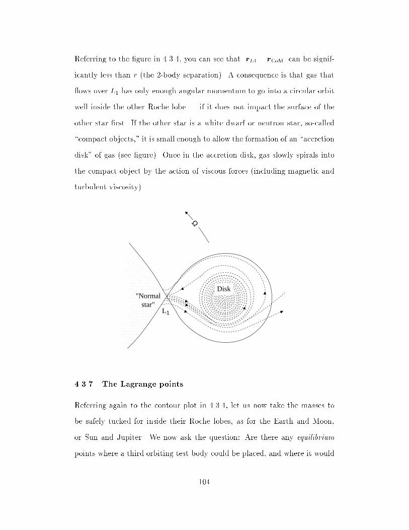
Referring to the gure in 4.3.4, you can see that jrL1 rCoMj can be signif-

icantly less than r (the 2-body separation). A consequence is that gas that

ows over L1 has only enough angular momentum to go into a circular orbit

well inside the other Roche lobe | if it does not impact the surface of the

other star rst. If the other star is a white dwarf or neutron star, so-called

\compact objects," it is small enough to allow the formation of an \accretion

disk" of gas (see gure). Once in the accretion disk, gas slowly spirals into

the compact object by the action of viscous forces (including magnetic and

turbulent viscosity).

Ω

DDskDisk"Normal

star"L1

4.3.7 The Lagrange points

Referring again to the contour plot in 4.3.4, let us now take the masses to

be safely tucked for inside their Roche lobes, as for the Earth and Moon,

or Sun and Jupiter. We now ask the question: Are there any equilibrium

points where a third orbiting test body could be placed, and where it would

104

maintain a constant position in the rotating frame (that is, co-orbit with the

same period as the two main bodies at constant position relative to them)?

The condition for such an equilibrium is that there be no acceleration

at the chosen position, that is, the gradient of the potential (including

centrifugal term) must vanish,

r = 0 :

Gradients vanish, in general, at extrema and at saddle points. In the contour

plot you can see that there are 3 saddlepoints co-linear with masses M1 and

M2. It is easy to see that there must always be these three (for any mass

ratio) as the following graph illustrates:

A B

O xL1 L2

L 3

Negative ofcentrifugal force

Gravitational force due to M1

Gravitational forcedue toM2

You can see that gravitational force and (negative) centrifugal force must

always cross at exactly three points, where

Fgrav = Fcentrif or Fgrav + Fcentrif = 0 :

These three points, L1; L2; L3 are the rst three \Lagrange points" where

a test mass can orbit. However, since they are saddle points (see contour

105

picture) all three are unstable: if the mass is slightly perturbed, it falls into

one of the potential wells or is ung o to innity.

More interesting are the two maxima of the potential, labelled L4 and L5

in the contour plot. These are the so-called stable Lagrange points. Looking

at the contour plot, or the surface plot at the beginning of 4.3, you can see

that these maxima occur along the ridge-line of a long, banana-shaped ridge

between the potential well of the combined masses and the centrifugal force

potential that decreases toward innity.

If a test mass is placed at L4 or L5, it will stay there. If it is perturbed

slightly, it will execute (in the rotating frame) a stable, though not necessarily

closed, orbit that goes around L4 or L5.

You might wonder how such an orbit can be stable if it is going around

a potential maximum, not minimum. The answer is that, in the rotating

frame, there is a Coriolis force ! v, so that a test particle's equation of

motion is actually

dv

dt= r ! v :

If ! in the contour picture is out of the page (M2 and M1 orbiting counter-

clockwise), then a particle pushed \outward" from L4 or L5 experiences a

clockwise force and goes into a small (stable) clockwise orbit around L4 or

L5 respectively.

The best real-life example of objects orbiting a stable Lagrange point

are the Trojan asteroids which orbit L4 and L5 of the Sun-Jupiter system.

Between 1906 and 1908, four such asteroids were found: the number has

now increased to several hundred (see gure). These asteroids are named

for the heroes from Homer's Iliad and are collectively called the Trojans.

Those that precede Jupiter (at L4) are named for the Greek heroes (plus the

106

Trojan spy, Hektor), and those that follow Jupiter (at L5) are named for the

Trojan warriors along with the Greek spy, Patroclus. Some of the Trojans

make complicated orbits taking as long as 140 years to meander around the

\banana" of the potential (meanwhile, of course, orbiting the Sun every 11.86

years, just like Jupiter). [Abell 7th Ed., 18.3]

We have not yet determined the location of L4 and L5 in the gure. The

amazing fact is that, independent of the mass ratio M1 :M2, L4 and L5 are

exactly at the vertices of equilateral triangles formed with M1 and M2. This

is so remarkable that we should at least verify it for fun:

107

mass m

F2F1

P

B

M2

6060R

r

ψ1

ψ2

CoM

A

M1pR p)R(1−

O

We want to see that F 1 + F 2 exactly balances the centrifugal term mr!2.

The magnitudes of F 1 and F 2 are

F1 =GmM1

R2=Gm(1 p)M

R2F2 =

GmM2

R2=GmpM

R2

where p M2=M1 and M = M1 +M2. So the condition for force balance

perpendicular to r is

F1 sin 1?= F2 sin 2 :

Apply the Law of Sines to the triangle AOP,

sin 60

r=

p3=2

r=

sin 1

pR:

108

So

sin 1 =p3pR=(2r)

and likewise using triangle BOP,

sin 2 =p3(1 p)R=(2r) :

Using the previous formulas for the magnitudes F1 and F2, the force check

becomes

F1 sin 1 =

p3pR

2r

G(1 p)M

R2

?=

p3(1 p)R

2r

GmpM

R2= F2 sin 2 :

Hey, it checks! So now we need to check the component parallel to r (which

includes the centrifugal term):

F1 cos 1 + F2 cos 2?= mr!2

Law of cosines on AOP:

cos 1 =r2 +R2 p2R2

2rR

Law of cosines on BOP:

cos 2 =r2 +R2 (1 p)2R2

2rR

Kepler's law:

!2 =GM

R3:

So "Gm(1 p)M

R2

# "r2 +R2 p2R2

2rR

#

+

GmpM

R2

"r2 +R2 (1 p)2R2

2rR

#?=

GMmr

R3

(1 p)(r2 +R2 p2R2) + p[r2 +R2 (1 p)2R2]

2r

?= r

r2 +R2(1 p+ p2)?= 2r2 :

109

Hmm. Is this true for all values of p? Yes! It is the Law of Cosines applied

to the triangle BOP (using cos 60 = 1=2):

r2 = R2 + (1 p)2R2 2(1 p)R2 cos 60

= R2(1 p+ p2) :

So the force balance is exact for both components.

4.4 The virial theorem

Many-body (that is, more than 2-body) dynamics is something that comes

later in the course, but we need to derive one important result, the virial

theorem, now. Just for fun, here is a fairly fancy derivation, taught to me by

George Rybicki. If this is above your level, just study it in a general way.

Suppose we have N bodies all interacting. Their kinetic energy is

T =1

2

NXi=1

miv2i

and their gravitational potential energy is

V = Xi6=j

Xj

Gmimj

jri rj j:

Newton's force law is

mi _vi = (rV )r=ri

:

Dene a quantity (a bit like a moment of inertia, but around a point, not an

axis)

I 1

2

NXi=1

mir2i :

Dierentiate with respect to time twice:

_I =Xi

mivi ri

110

I =Xi

mi _vi ri +Xi

mivi vi

= Xi

ri (rV )r=ri+ 2T :

Now here is the tricky part: The virial theorem comes about because the

potential energy V has a scaling relation that describes how its numerical

value would change if all positions r were stretched by some factor . In

particular, you can see right away that

V (r1; r2; : : : ; rN) =1

V (r1; r2; : : : ; rN ) :

Dierentiating with respect to , and then setting = 1, we get

Xi

ri (rV )r=ri= V :

Thus

I = V + 2T :

This is called the time dependent virial theorem. It says, roughly, that if

V +2T > 0, the mean square size of the systemmust eventually be increasing

while if V +2T < 0 the size must eventually be decreasing. (Remember that

V is negative, for this to make sense.)

It also follows, logically enough, that if a gravitating system is in equilib-

rium, neither increasing nor decreasing steadily in size, it must have

hV + 2T i = 0 or 2hT i = hV i :

Here the angle brackets denote the long-time average. To see this formally,

average the time dependent theorem over a long time T :

hV + 2T i = 1

T

Z T

0(V + 2T ) dt =

1

T

Z T

0

I dt =1

T[ _I(T ) _I(0)] :

111

Now if all particles remain bounded with bounded velocities for all time

(the denition of an equilibrium system) then _I(t) remains bounded (see its

formula above) and the right hand side goes to zero as T !1, thus proving

the desired time-averaged virial theorem.

112