Embed Size (px)
Citation preview
Physics of Classical Electromagnetism

Minoru Fujimoto
Physics of ClassicalElectromagnetism
Minoru FujimotoDepartment of PhysicsUniversity of GuelphGuelph, OntarioCanada, N1G 2W1
Library of Congress Control Number: 2007921094
ISBN: 978-0-387-68015-6 e-ISBN: 978-0-387-68018-7
Printed on acid-free paper.
C© 2007 Springer Science+Business Media, LLCAll rights reserved. This work may not be translated or copied in whole or in part without the writtenpermission of the publisher (Springer Science+Business Media, LLC, 233 Spring Street, New York,NY 10013, USA), except for brief excerpts in connection with reviews or scholarly analysis. Usein connection with any form of information storage and retrieval, electronic adaptation, computersoftware, or by similar or dissimilar methodology now known or hereafter developed is forbidden.The use in this publication of trade names, trademarks, service marks, and similar terms, even if theyare not identified as such, is not to be taken as an expression of opinion as to whether or not they aresubject to proprietary rights.
9 8 7 6 5 4 3 2 1
springer.com
Contents
Preface.................................................................................... xi
1. Steady Electric Currents ......................................................... 11.1. Introduction .................................................................. 11.2. Standards for Electric Voltages and Current ........................... 21.3. Ohm Law’s and Heat Energy ............................................. 41.4. The Kirchhoff Theorem.................................................... 8
PART 1. ELECTROSTATICS 13
2. Electrostatic Fields................................................................ 152.1. Static Charges and Their Interactions ................................... 152.2. A Transient Current and Static Charges ................................ 162.3. Uniform Electric Field in a Parallel-Plate Condenser ................ 19
2.3.1. The Electric Field Vector ......................................... 192.3.2. The Flux Density Vector .......................................... 21
2.4. Parallel and Series Connections of Capacitors ........................ 252.5. Insulating Materials ........................................................ 26
3. The Gauss Theorem .............................................................. 303.1. A Spherical Capacitor...................................................... 303.2. A Cylindrical Capacitor ................................................... 333.3. The Gauss Theorem ........................................................ 343.4. Boundary Conditions....................................................... 39
3.4.1. A Conducting Boundary .......................................... 393.4.2. A Dielectric Boundary ............................................ 40
4. The Laplace–Poisson Equations................................................ 434.1. The Electrostatic Potential ................................................ 434.2. The Gauss Theorem in Differential Form .............................. 444.3. Curvilinear Coordinates (1) ............................................... 46
v
vi Contents
4.4. The Laplace–Poisson Equations ......................................... 494.4.1. Boundary Conditions .............................................. 494.4.2. Uniqueness Theorem .............................................. 504.4.3. Green’s Function Method......................................... 51
4.5. Simple Examples............................................................ 534.6. The Coulomb Potential .................................................... 554.7. Point Charges and the Superposition Principle........................ 58
4.7.1. An Electric Image .................................................. 584.7.2. Electric Dipole Moment........................................... 604.7.3. The Dipole-Dipole Interaction................................... 63
5. The Legendre Expansion of Potentials ........................................ 645.1. The Laplace Equation in Spherical Coordinates ...................... 645.2. Series Expansion of the Coulomb Potential............................ 665.3. Legendre’s Polynomials ................................................... 685.4. A Conducting Sphere in a Uniform Field .............................. 695.5. A Dielectric Sphere in a Uniform Field................................. 715.6. A Point Charge Near a Grounded Conducting Sphere ............... 725.7. A Simple Quadrupole ...................................................... 755.8. Associated Legendre Polynomials ....................................... 765.9. Multipole Potentials ........................................................ 79
PART 2. ELECTROMAGNETISM 83
6. The Ampere Law.................................................................. 856.1. Introduction .................................................................. 856.2. The Ampere Law............................................................ 866.3. A Long Solenoid ............................................................ 896.4. Stokes’ Theorem ............................................................ 916.5. Curvilinear Coordinates (2) ............................................... 946.6. The Ampere Law in Differential Form.................................. 966.7. The Rowland Experiment ................................................. 98
7. Magnetic Induction ............................................................... 1017.1. Laws of Magnetic Induction .............................................. 101
7.1.1. The Faraday Law................................................... 1017.1.2. The Lenz Law....................................................... 1037.1.3. Magnetic Field Vectors............................................ 103
7.2. Differential Law of Induction and the Dynamic Electric Field..... 1047.3. Magnetic Moments ......................................................... 108
8. Scalar and Vector Potentials..................................................... 1128.1. Magnets....................................................................... 1128.2. Pohl’s Magnetic Potentiometer........................................... 114
Contents vii
8.3. Scalar Potentials of Magnets ............................................ 1168.3.1. A Laboratory Magnet........................................... 1168.3.2. A Uniformly Magnetized Sphere............................. 118
8.4. Vector Potentials........................................................... 1198.5. Examples of Steady Magnetic Fields .................................. 1218.6. Vector and Scalar Potentials of a Magnetic Moment ............... 1268.7. Magnetism of a Bohr’s Atom ........................................... 128
9. Inductances and Magnetic Energies ........................................... 1329.1. Inductances ................................................................. 1329.2. Self- and Mutual Inductances ........................................... 1359.3. Mutual Interaction Force Between Currents.......................... 1389.4. Examples of Mutual Induction.......................................... 139
9.4.1. Parallel Currents................................................. 1399.4.2. Two Ring Currents .............................................. 140
10. Time-Dependent Currents ...................................................... 14210.1. Continuity of Charge and Current...................................... 14210.2. Alternating Currents ...................................................... 14310.3. Impedances ................................................................. 14510.4. Complex Vector Diagrams............................................... 14710.5. Resonances ................................................................. 149
10.5.1. A Free LC Oscillation .......................................... 14910.5.2. Series Resonance ............................................... 15010.5.3. Parallel Resonance .............................................. 151
10.6. Four-Terminal Networks ................................................. 15210.6.1. RC Network ...................................................... 15310.6.2. Loaded Transformer ............................................ 15510.6.3. An Input-Output Relation in a Series RCL Circuit........ 15610.6.4. Free Oscillation in an RCL Circuit .......................... 157
PART 3. ELECTROMAGNETIC WAVES 159
11. Transmission Lines ............................................................... 16111.1. Self-Sustained Oscillators ............................................... 16111.2. Transmission Lines........................................................ 16311.3. Fourier Transforms........................................................ 16511.4. Reflection and Standing Waves ......................................... 16711.5. The Smith Chart ........................................................... 170
12. The Maxwell Equations ......................................................... 17212.1. The Maxwell Equations .................................................. 17212.2. Electromagnetic Energy and the Poynting Theorem................ 17512.3. Vector and Scalar Potentials............................................. 176
viii Contents
12.4. Retarded Potentials........................................................ 17712.5. Multipole Expansion...................................................... 180
13. Electromagnetic Radiation ...................................................... 18413.1. Dipole Antenna ............................................................ 18413.2. Electric Dipole Radiation ................................................ 18413.3. The Hertz Vector .......................................................... 18813.4. A Half-Wave Antenna .................................................... 19213.5. A Loop Antenna ........................................................... 19313.6. Plane Waves in Free Space .............................................. 195
14. The Special Theory of Relativity............................................... 19914.1. Newton’s Laws of Mechanics........................................... 19914.2. The Michelson–Morley Experiment ................................... 20014.3. The Lorentz Transformation ............................................ 20214.4. Velocity and Acceleration in Four-Dimensional Space ............ 20414.5. Relativistic Equation of Motion ........................................ 20614.6. The Electromagnetic Field in Four-Dimensional Space............ 208
15. Waves and Boundary Problems................................................. 21415.1. Skin Depths................................................................. 21415.2. Plane Electromagnetic Waves in a Conducting Medium........... 21615.3. Boundary Conditions for Propagating Waves........................ 21815.4. Reflection from a Conducting Boundary.............................. 21915.5. Dielectric Boundaries..................................................... 22115.6. The Fresnel Formula...................................................... 223
16. Guided Waves...................................................................... 22616.1. Propagation Between Parallel Conducting Plates ................... 22616.2. Uniform Waveguides ..................................................... 229
16.2.1. Transversal Modes of Propagation(TE and TM Modes)............................................ 229
16.2.2. Transversal Electric-Magnetic Modes (TEM) ............. 23216.3. Examples of Waveguides ................................................ 233
PART 4. COHERENT WAVES AND RADIATION QUANTA 241
17. Waveguide Transmission ........................................................ 24317.1. Orthogonality Relations of Waveguide Modes....................... 24317.2. Impedances ................................................................. 24517.3. Power Transmission Through a Waveguide .......................... 24917.4. Multiple Reflections in a Waveguide .................................. 250
18. Resonant Cavities ................................................................. 25318.1. Slater’s Theory of Normal Modes...................................... 25318.2. The Maxwell Equations in a Cavity.................................... 256

Contents ix
18.3. Free and Damped Oscillations .......................................... 25818.4. Input Impedance of a Cavity ............................................ 26018.5. Example of a Resonant Cavity.......................................... 26318.6. Measurements of a Cavity Resonance................................. 265
19. Electronic Excitation of Cavity Oscillations ................................. 26819.1. Electronic Admittance.................................................... 26819.2. A Klystron Cavity ......................................................... 27019.3. Velocity Modulation ...................................................... 27419.4. A Reflex Oscillator........................................................ 276
20. Dielectric and Magnetic Responses in Resonant Electromagnetic Fields 28020.1. Introduction................................................................. 28020.2. The Kramers–Kronig Formula.......................................... 28120.3. Dielectric Relaxation ..................................................... 28320.4. Magnetic Resonance ..................................................... 28820.5. The Bloch Theory ......................................................... 29020.6. Magnetic Susceptibility Measured by Resonance Experiments .. 292
21. Laser Oscillations, Phase Coherence, and Photons ......................... 29421.1. Optical Resonators ........................................................ 29421.2. Quantum Transitions...................................................... 29621.3. Inverted Population and the Negative Temperature ................. 29921.4. Ammonium Maser ........................................................ 30021.5. Coherent Light Emission from a Gas Laser .......................... 30121.6. Phase Coherence and Radiation Quanta .............................. 302
APPENDIX 305
Mathematical Notes .................................................................... 307A.1. Orthogonal Vector Space....................................................... 307A.2. Orthogonality of Legendre’s Polynomials .................................. 308A.3. Associated Legendre Polynomials............................................ 310A.4. Fourier Expansion and Wave Equations..................................... 312A.5. Bessel’s Functions ............................................................... 314
REFERENCES 317
Index ...................................................................................... 319
Preface
The Maxwell theory of electromagnetism was well established in the latter nine-teenth century, when H. R. Hertz demonstrated the electromagnetic wave. Thetheory laid the foundation for physical optics, from which the quantum conceptemerged for microscopic physics. Einstein realized that the speed of electromag-netic propagation is a universal constant, and thereby recognized the Maxwellequations to compose a fundamental law in all inertial systems of reference. Onthe other hand, the pressing demand for efficient radar systems during WWIIaccelerated studies on guided waves, resulting in today’s advanced telecommuni-cation technology, in addition to a new radio- and microwave spectroscopy. Thestudies were further extended to optical frequencies, and laser electronics and so-phisticated semi-conducting devices are now familiar in daily life. Owing to theseadvances, our knowledge of electromagnetic radiation has been significantly up-graded beyond plane waves in free space. Nevertheless, in the learning processthe basic theory remains founded upon early empirical rules, and the traditionalteaching should therefore be modernized according to priorities in the modern era.
In spite of the fact that there are many books available on this well-establishedtheme, I was motivated to write this book, reviewing the laws in terms of contem-porary knowledge in order to deal with modern applications. Here I followed twobasic guidelines. First, I considered electronic charge and spin as empirical in thedescription of electromagnetism. This is unlike the view of early physicists, whoconsidered these ideas hypothetical. Today we know they are factual, althoughstill unexplained from first principle. Second, the concept of “fields” should be inthe forefront of discussion, as introduced by Faraday. In these regards I benefitedfrom Professor Pohl’s textbook, Elektrizitatslehre, where I found a very stimu-lating approach. Owing a great deal to him, I was able to write my introductorychapters in a rather untraditional way, an approach I have found very useful inmy classes. In addition, in this book I discussed microwave and laser electronicsin some depth, areas where coherent radiation plays a significant role for moderntelecommunication.
I wrote this book primarily for students at upper undergraduate levels, hopingit would serve as a useful reference as well. I emphasized the physics of elec-tromagnetism, leaving mathematical details to writers of books on “mathematical
xi

xii Preface
physics.” Thus, I did not include sections for “mathematical exercise,” but I hopethat readers will go through the mathematical details in the text to enhance theirunderstanding of the physical content.
In Chapter 21 quantum transitions are discussed to an extent that aims to makeit understandable intuitively, although here I deviated from classical theories.Although this topic is necessary for a reader to deal with optical transitions, myintent was to discuss the limits of Maxwell’s classical theory that arise from phasecoherency in electromagnetic radiation.
It is a great pleasure to thank my students and colleagues, who assisted me bytaking part in numerous discussions and criticisms. I have benefited especially bycomments from S. Jerzak of York University, who took time to read the first draft.I am also grateful to J. Nauheimer who helped me find literature in the Germanlanguage. My appreciation goes also to Springer-Verlag for permission to use somefigures from R. W. Pohl’s book Elektrizitatslehre.
Finally, I thank my wife Haruko for her encouragement during my writing,without which this book could not have been completed.
M. FujimotoSeptember 2006

1Steady Electric Currents
1.1. Introduction
The macroscopic electric charge on a body is determined from the quantity ofelectricity carried by particles constituting the material. Although some electricphenomena were familiar before discoveries of these particles, such an origin ofelectricity came to our knowledge after numerous investigations of the structureof matter. Unlike the mass that represents mechanical properties, two kinds ofelectric charges different in sign were discovered in nature, signified by attractiveand repulsive interactions between charged bodies. While electric charges can becombined as in algebraic addition, carrier particles tend to form neutral species inequilibrium states of matter, corresponding to zero of the charge in macroscopicscale.
Frictional electricity, for example, represents properties of rubbed bodies arisingfrom a structural change on the surfaces, which is unrelated to their masses. Also,after Oersted’s discovery it was known that the magnetic field is related to movingcharges. It is well established that electricity and magnetism are not independentphenomena, although they were believed to be so in early physics. Today, suchparticles as electrons and atomic nuclei are known as basic elements composedof masses and charges of materials, as substantiated in modern chemistry. Theelectromagnetic nature of matter can therefore be attributed to these particleswithin accuracies of modern measurements. In this context we can express the lawof electromagnetism more appropriately than following in the footsteps in earlyphysics.
Today, we are familiar with various sources of electricity besides by friction.Batteries, for example, a modern version of Volta’s pile1, are widely used in dailylife as sources of steady electric currents. Also familiar is alternating current (AC)that can be produced when a mechanical work is converted to an induction currentin a magnetic field. Supported by contemporary chemistry, in all processes where
1 Volta’s pile was constructed in multi-layers of Zn and Cu plates sandwiched alternatelywith wet rags. Using such a battery, he was able to produce a relatively high emf for a weakcurrent by today’s standard.
1
2 1. Steady Electric Currents
electricity is generated, we note that positive and negative charges are separatedfrom neutral matter at the expense of internal and external energies. Positive andnegative charges ±Q are thus produced simultaneously in equal quantities, wherethe rate dQ/dt , called the electric current, is a significant quantity for electricalenergies to be used for external work. Traditionally, the current source is charac-terized by an electromotive force, or “emf,” to signify the driving force, which isnow expressed by the potential energy of the source.
Historically, Volta’s invention of an electric pile (ca. 1799) played an importantrole in producing steady currents, which led Oersted and Ampere to discoveries ofthe fundamental relation between current and magnetic fields (1820). In such earlyexperiments with primitive batteries, these pioneers found the law of the magneticfield by using small compass needles placed near the current. Today, the magneticfield can be measured with an “ammeter” that indicates an induced current. Inaddition to the electron spin discovered much later, it is now well established thatcharges in motion are responsible for magnetic fields, and all electrical quantitiescan be expressed in practical units of emf and current. As they are derived fromprecision measurements, these units are most suitable for formulating the laws ofelectromagnetism.
On the other hand, energy is a universal concept in physics, and the unit “joule,”expressed by J in the MKS system2, is conveniently related to practical electricalunits. In contrast, traditional CGS units basically contradict the modern view ofelectricity, namely, that it is independent from mechanical properties of matter.
In classical physics, the electrical charge is a macroscopic quantity. Needlessto say, it is essential that such basic quantities be measurable with practical in-struments such as the aforementioned ammeter and the voltmeter; although thedetailed construction of meters is not our primary concern in formulating the laws,these instruments allow us to set the standard for currents and emf’s.
1.2. Standards for Electric Voltages and Current
Electric phenomena normally observed in the laboratory scale originate from thegross behavior of electrons and ions in metallic conductors and electrolytic solu-tions. It is important to realize that the electronic charge is the minimum quantityof electricity in nature under normal circumstances3. The charge on an electronhas been measured to great accuracy: e = −(1.6021892 ± 0.000029) × 10−19 C,where C is the practical MKS unit “coul.”
2 MKS stands for meter-kilogram-second, representing basic units of length, mass, andtime, respectively. Electric units can be defined in any system in terms of these units formechanical quantities, however, in the MKSA system, the unit ampere for an electric currentis added as independent of mass and space-time. CGS units are centimeter, gram, and second,representing mass and space-time similar to MKS system.3 According to high-energy physics, charged particles bearing a fraction of the electroniccharge, such as e/2 and e/3, called “quarks” have been identified. However, these particlesare short-lived, and hence considered as insignificant for classical physics.
Standards for Electric Voltages and Current 3
In a battery, charges +Q and −Q are produced by internal chemical reactionsand accumulate at positive and negative electrodes separately. Placed between andin contact with these electrodes, certain materials exhibit a variety of conductingbehaviors. Many materials can be classified into two categories: conductors andinsulators, although some exhibit a character between these two categories. Metals,e.g., copper and silver, are typical conductors, whereas mica and various ceramicsare good insulators. Microscopically, these categories can be characterized bythe presence or absence of mobile electrons in materials, where mobile particlesare considered to be moved by charges ±Q on the electrodes. As mentioned,traditionally, such a driving force for mobile charges was called an electromotiveforce and described as a force F proportional to Q, although differentiated froma voltage difference defined for a battery. Mobile electrons in metals are by nomeans “free,” but moved by F , drifting against an internal frictional force Fd. Fordrift motion at a steady rate, the condition F + Fd = 0 should be met, giving riseto what is called a steady current.
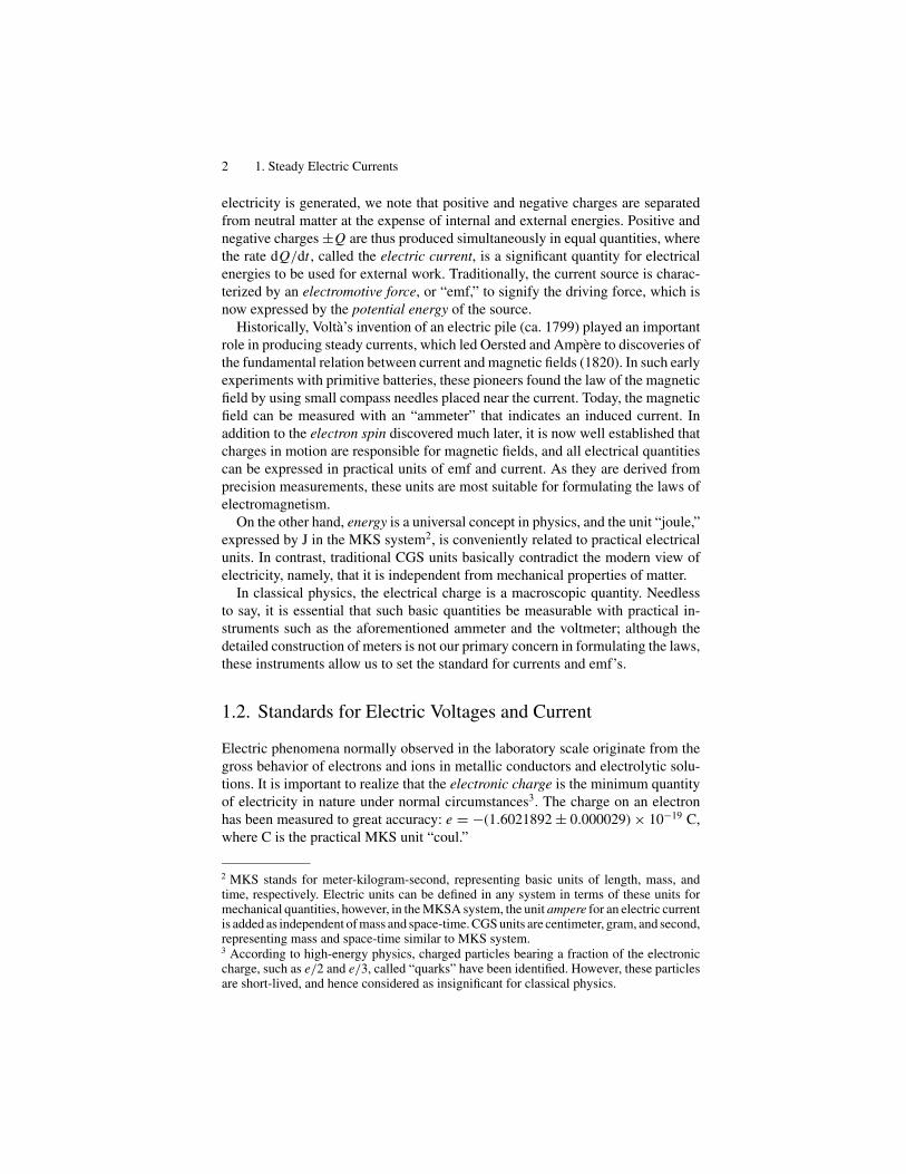
For ionic conduction in electrolytic solutions, Faraday discovered the law ofelectrolysis (1833), presenting his view of the ionic current. Figure 1.1 shows asteady electrolysis in a dilute AgNO3 solution, where a mass MAg of depositedsilver on the negative electrode is proportional to the amount of charge q transportedduring a time t , that is,
MAg ∝ q. (1.1)
The mass MAg can be measured in precision in terms of molar number N ofAg+, hence the transported charge q can be expressed by the number N that isproportional to the time t for the electrolysis.
FIGURE 1.1. Electrolysis of AgNO3
solution.

4 1. Steady Electric Currents
With accurately measured MAg and t , the current I = q/t can be determinedin great precision. Using an electrolytic cell, a current that deposits 1.1180 mg ofsilver per second is defined as one ampere (1A). Referring to the current of 1A,the unit for a charge is called 1 coulomb, i.e., 1C = 1A-sec.
To move a charge q through a connecting wire, the battery must supply an energyW that should be proportional to q, and therefore we define the quantity V = W/q,called the potential or electric potential. The MKS unit for W is J, so that the unitof V can be specified by J-C−1, which is called a “volt” and abbreviated as V.
In the MKS unit system the ampere (A) for a current is a fundamental unit,whereas “volt” is a derived unit from ampere. Including A as an additional basicunit, the unit system is referred to as the “MKSA system.” Nevertheless, a cadmiumcell, for example, provides an excellent voltage standard: Vemf = 1.9186 × 0.0010V with excellent stability 1�V/yr under ambient conditions.
A practical passage of a current is called a circuit, connecting a battery andanother device with conducting wires. For a steady current that is time-independent,we consider that each point along a circuit can be uniquely specified by an electricpotential, and a potential difference between two points is called voltage. Thepotential V is a function of a point x along the circuit, and the potential differenceV (+) − V (−) between terminals + and − of a battery is equal to the emf voltage,Vemf. If batteries are removed from a circuit, there is, naturally, no current; thepotentials are equal at all points in the circuit—that is, V (x) = const in the absenceof currents.
1.3. Ohm Law’s and Heat Energy
Electric conduction takes place through conducting materials, constituting a majorsubject for discussion in solid state physics. In the classical description we consideronly idealized conductors, either metallic or electrolytic. In the former electrons arecharge carriers, whereas in the latter both positive and negative ions are mobile,contributing to the electrolytic current. These carriers can drift in two oppositedirections; however, the current is defined for expressing the amount of charges|Q| transported per unit time, which is basically a scalar quantity, as will beexplained in the following discussion. In this context how to specify the currentdirection is a matter of convenience. Normally, the current is considered to flowin the direction for decreasing voltage, namely from a higher to a lower voltage.
Because it is invisible the current is “seen” by three major effects, of whichmagnetic and chemical effects have already been discussed. The third effect is heatproduced by currents in a conducting passage, for which Ohm (1826) discoveredthe basic law of electrical resistance. Joule (ca. 1845) showed later that heatproduced by a current is nothing but dissipated energy in a conductor.
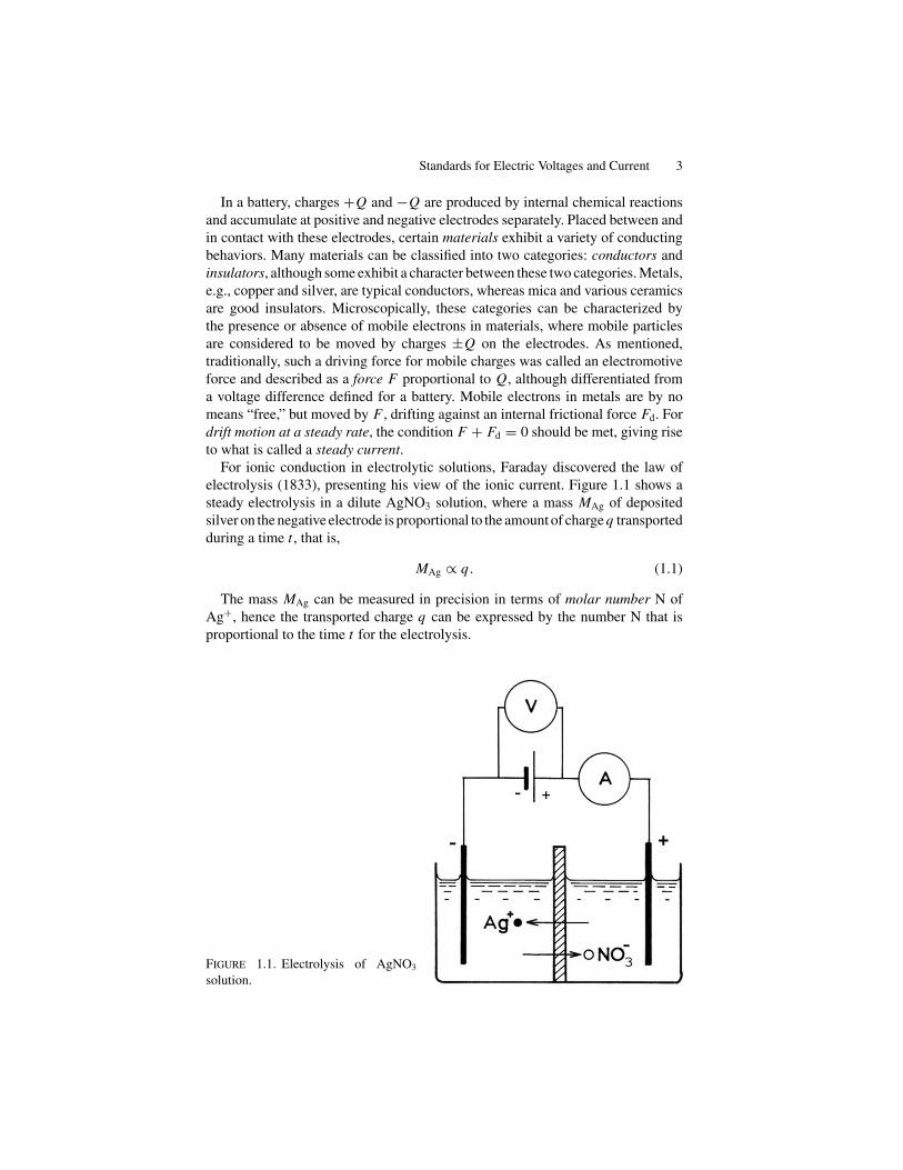
Consider a long conducting wire of a uniform cross-sectional area S. Figure 1.2illustrates a steady flow of electrons through a cylindrical passage, where weconsider a short cylindrical volume S�x between x − �x and x along the wire.
Ohm Law’s and Heat Energy 5
FIGURE 1.2. A simplified model for electronic conduction.
For a steady flow we can assume that the carrier density n is a constant oftime between these points, at which the corresponding times are t − �t and t ,respectively. If the potential is assumed to be higher to the left and lower to theright, the current should flow from the left to the right, as indicated in the figure.Assuming also that all electrons move in the direction parallel to the wire, theamount of charge �Q = neS�x can be considered to move in and then out of thevolume S�x during the time interval �t , where e < 0 is the negative electroniccharge. Therefore, the current is expressed as
I = �Q
�t= neS
�x
�t= nevdS (1.2)
where vd = �x/�t is the drift velocity of electrons. We can therefore write
I = jS, where j = nevd, (1.3)
called the current density in the area S. It is noted from (1.3) that the sign ofj depends on the direction of vd. For negative electrons, e < 0, the current ispositive, I > 0, if vd < 0. For an ionic conduction of positive and negative carri-ers whose charges are e1 > 0 and e2 < 0, respectively, the equation (1.3) can begeneralized as
j = n1e1v1 + n2e2v2, (1.4)
where both terms on the right give positive contributions to j , despite the fact thations 1 and 2 drift in opposite directions.
In the above simple model, the current density for a steady flow may not besignificant, but for a distributed current it is an important measure, as will bediscussed later for a general case. The MKSA unit of a current density is given by[ j] = A-m−2 = C-m−2-s−1.
Next, we consider the potential difference between x − �x and x , which isresponsible for the current through these points. For a small �x , the potential

6 1. Steady Electric Currents
difference �V can be calculated as
�V = V (x − �x) − V (x) = −F�x,
where the quantity F = −�V/�x represents the driving force for a hypotheticalunit charge 1C. Nevertheless, there is inevitably a frictional force in the conductingmaterial, as can be described by Hooke’s law in mechanics, expressed by Fd =−kvd, where k is an elastic constant.
For a steady current, we have F = −Fd, and therefore we can write
�V = Fd�x = kv d�x .
Eliminating vd from this expression and (1.2), we obtain
�V = �RI, where �R =(
k
neS
)�x,
the electrical resistance between x − �x and x . For a uniform wire, this resultcan be integrated to obtain the total resistance from the relation, that is,
−∫ B
A
dV = V (A) − V (B) = Vemf = I k
neS
∫ L
0
dx = RI ,
where
R = kL
neS= �
L
S(1.5)
is the resistance formula for a uniform conductor that can be calculated as the
length L and cross-sectional area S are specified. The constant � = k
neis called the
resistivity, and its reciprocal 1/� = � is the conductivity of the material. Writinga potential difference and resistance between two arbitrary points as �V and R,Ohm’s law can be expressed as
�V = RI . (1.6)
Obviously, the current occurs if there is a potential difference in a circuit. Thatis, if no current is present the conductor is static and characterized by a constantpotential at all points. Values of � listed in Tables 1.1 and 1.2 are for representativeindustrial materials useful for calculating resistances.
The current loses its energy when flowing through a conducting material, asevidenced by the produced heat. Therefore, to maintain a steady current, the con-nected battery should keep producing charges at the expense of stored energy inthe battery. Although obvious by what we know today, the energy relation for heatgeneration was first verified by Joule (ca. 1845), who demonstrated equivalenceof heat and energy.
Figure 1.3 shows Joule’s experimental setup. To flow a current I through theresistor R, a battery of Vemf performs work. The work to drive a charge �Q outof the battery is expressed by �W = Vemf�Q, and hence we can write �W =(RI)�Q, using Ohm’s law.

Ohm Law’s and Heat Energy 7
TABLE 1.1. Electrical resistivities of metals
Metals Temp, ◦C � × 10−8 �m � × 10−3 Metals Temp, ◦C � × 10−8 �m � × 10−3
Ag 20 1.6 4.1 Mg 20 4.5 4.0
Al 20 2.75 4.2 Mo 20 5.6 4.4
As 20 35 3.9 Na 20 4.6 5.5
Au 20 2.4 4.0 Ni 20 7.24 6.7
Be 20 6.4 −78 3.9
Bi 20 120 4.5 Os 20 9.5 4.2
Ca 20 4.6 3.3 Pb 20 21 4.2
Cd 20 7.4 4.2 Pd 20 10.8 3.7
Co 0 6.37 6.58 Pt 20 10.6 3.9
Cr 20 17 1000 43
Cs 20 21 4.8 −78 6.7
Cu 20 1.72 4.3 Rb 20 12.5 5.5
100 2.28 Rd 20 5.1 4.4
−78 1.03 Sb 0 38.7 5.4
−183 0.30 Sr 0 30.3 3.5
Fe (pure) 20 9.8 6.6 Th 20 18 2.4
−78 4.9 Tl 20 19 5
Hg 0 94.08 0.99 W 20 5.5 5.3
20 95.8 1000 35
In 0 8.2 5.1 3000 123
Ir 20 6.5 3.9 −78 3.2
K 20 6.9 5.1 Zn 20 11.4 4.5
Li 20 9.4 4.6 Zr 20 49 4.0
The temperature coefficient � of a resistivity is defined as � = (�100 − �0)/100�0 between 0 and
100◦C. From Rika Nenpyo (Maruzen, Tokyo 1962).
Because of the relation �Q = I�t , we obtain �W = (RI2)�t , and hence thepower delivered by the battery is expressed by
P = RI 2 = V 2emf
R= Vemf I. (1.7)
In Joule’s experiment, the resistor R was immersed in a water bath that wasthermally insulated from outside, where the heat produced in R was detected
TABLE 1.2. Electrical resistivities of alloys∗
Alloys (◦C) � × 10−8�� � × 10−3
Alumel (0) 33 1.2
Invar (0) 75 2
Chromel 70–110 0.11–0.54
Brass 5–7 1.4–2.0
Bronze 13–18 0.5
Nichrome (20) 109 0.10
German silver 17–41 0.04–0.38
Phos. bronze 2–6
∗From Rika Nenpyo, (Maruzen, Tokyo, 1962).

8 1. Steady Electric Currents
FIGURE 1.3. A set-up for Joule’s experiment.
by the thermometer immersed in the water. Joule showed that the energy deliv-ered by the battery, i.e., �W = P�t , was equal to the product C��, where Cis the heat capacity of water bath, and ��. the observed temperature rise. From(1.7), the unit of power—the watt (W)—is given by the electrical units of volt× ampere, making the MKSA system more practical than the traditional CGSsystem.
Owing to Joule’s experiment, a traditional unit for heat—“calorie” (cal)—is nolonger necessary, replaced by “joule”(J) although “calorie” and “kilocalorie” arestill familiar units in biological and chemical sciences. The conversion between Jand cal can be made by the relation 1 cal = 4.184 J. With the Ohm law, the MKSAunit of a resistance R is V-A−1, which is called “ohm”, and expressed as �
1.4. The Kirchhoff Theorem
In an electric circuit, a battery is a current source in conducting resistors, providingdistributed potentials V (x) along the circuit. In a simple circuit where a battery ofVemf is connected with one resistor R, the Ohm law Vemf = RI can be interpreted

The Kirchhoff Theorem 9
to mean that the current I circulates in the direction from the positive terminal tothe negative terminal along a closed loop circuit of Vemf and R. In this descriptionthe current direction inside the battery is opposite to the current direction in theresistance; however such a contradiction can be disregarded if we consider thatthe mechanism inside the battery is not our primary concern. Kirchhoff (1849)extended such an interpretation to more general circuits consisting of many emf’sand resistors, and formulated the general theorem to deal with currents throughthese resistors.
In a steady-current condition, we consider that the potential V (x) is signified bya unique value at any point x along the current passage, whereas at specific pointsxi where batteries are installed, we consider discontinuous voltages Vemf(xi). Asteady current Ij can flow through each resistor Rj that are indexed j = 1, 2, . . . ,
but the current direction and the potential difference across Rj can be left asprimarily unknown. Also in a circuit are junctions in the current passage, indexedby k = 1, 2, . . . , where more than two currents are mixed.
For a general circuit, we can consider several closed loops, �, �, . . . , which canbe either part of the circuit or can make up the whole circuit. It is significant thatV (x) takes a unique value at any given point x , so that the potential value shouldbe the same, no matter how the current circulates along a closed loop in eitherdirection. Mathematically, this can be expressed by
∮C dV = 0 along any of these
loops C of a given circuit, for which we can write∑i
Vemf (xi) =∑
j
Rj Ij. (1.8)
Known as the Kirchhoff theorem, (1.8) can be applied to any closed loop inthe circuit. Next, at any junction k of steady currents, we note that total incomingcurrents must be equal to total outgoing currents, namely, there is no accumulatedcharge at the point k; that is the law of current continuity. Assuming all directionsof currents exist arbitrarily at the junction, we must have the relation∑
k
Ik = 0 (1.9)
at all junctions, which is known as Kirchhoff’s junction theorem. As these currentsare primarily unknown, we can usually assume their directions for solving equa-tions (1.8) and (1.9); the assumed current directions are then corrected by signs ofthe solutions.
We solve (1.8) and (1.9) as a set of algebraic equations for unknown currentsIj, j = 1, 2, . . . . However, all of these equations are not required, and hence wecan select equations to solve sufficiently for the given number j of Rj, as shown bythe following examples.
Example 1. Two Resistances in Series Connection.Figure 1.4(a) shows a circuit, where two resistors R1 and R2 are connected in
series with a battery of Vemf. In a steady current condition, the points A, B, and Care signified by unique potentials VA, VB, and VC, respectively.
10 1. Steady Electric Currents
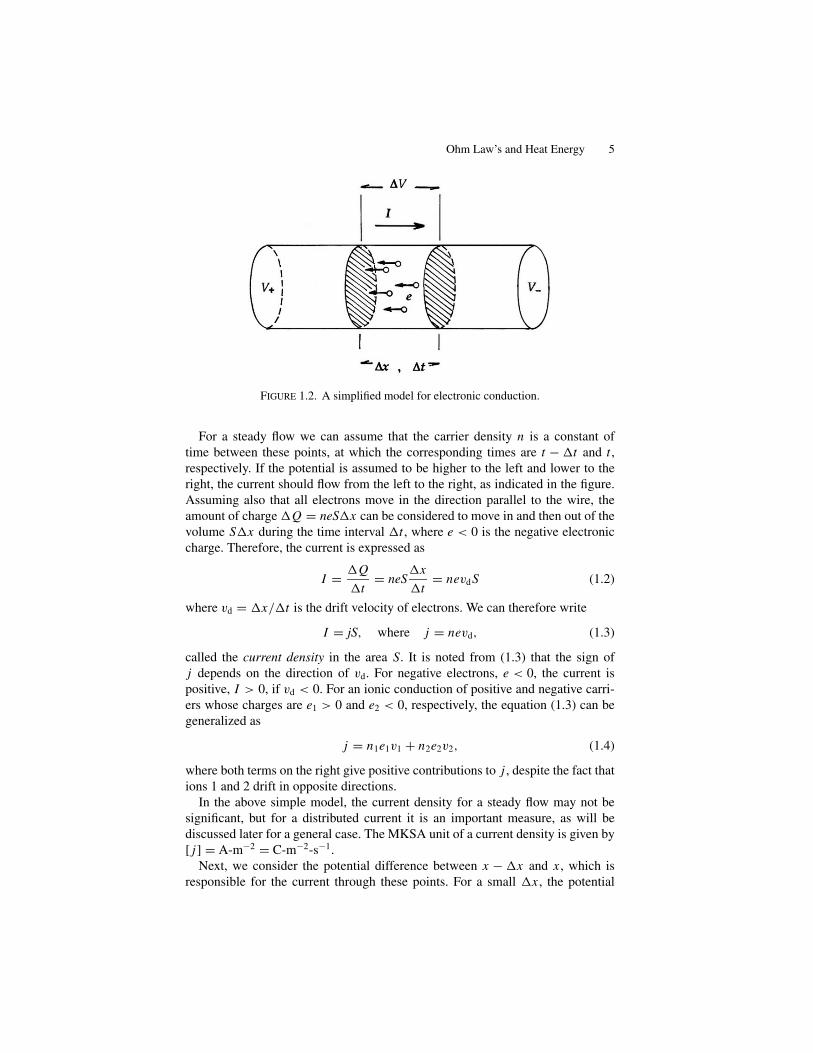
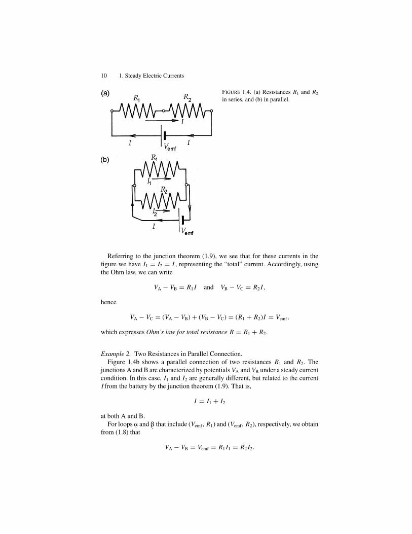
FIGURE 1.4. (a) Resistances R1 and R2
in series, and (b) in parallel.
Referring to the junction theorem (1.9), we see that for these currents in thefigure we have I1 = I2 = I , representing the “total” current. Accordingly, usingthe Ohm law, we can write
VA − VB = R1 I and VB − VC = R2 I,
hence
VA − VC = (VA − VB) + (VB − VC) = (R1 + R2)I = Vemf,
which expresses Ohm’s law for total resistance R = R1 + R2.
Example 2. Two Resistances in Parallel Connection.Figure 1.4b shows a parallel connection of two resistances R1 and R2. The
junctions A and B are characterized by potentials VA and VB under a steady currentcondition. In this case, I1 and I2 are generally different, but related to the currentI from the battery by the junction theorem (1.9). That is,
I = I1 + I2
at both A and B.For loops �. and �. that include (Vemf, R1) and (Vemf, R2), respectively, we obtain
from (1.8) that
VA − VB = Vemf = R1 I1 = R2 I2.

The Kirchhoff Theorem 11
FIGURE 1.5. Kirchhoff’s theorems. Junctions A and B, loops ABC, ADB, and CDB are
named �, �, and � , respectively.
Solving these equations for I1 and I2, we obtain
I =(
1
R1
+ 1
R2
)Vemf,
and the total resistance R in parallel connections can be determined from
1
R= 1
R1
+ 1
R2
.
Example 3. Calculation of currents in a circuit shown in Figure 1.5. In this cir-cuit, three loops �, �, and � and two junctions A and B can be consideredfor Kirchhoff’s theorem, as shown in the figure; however, we only need threeequations to solve (1.8) and (1.9) for I1, I2, and I3. Also, to set up three equa-tions, the directions of currents can be assumed arbitrarily, as indicated in thefigure.
Here, we apply (1.8) to the loops �, and �, and (1.9) to the junction A. Referringto assigned current directions, we can write three equations, respectively, for �, �,and A, which are
I1 R1 + (−I2)R2 + Va = 0,
(−I1)R1 + (−I3)R3 + (−Vb) = 0,

12 1. Steady Electric Currents
and
I1 + I2 + (−I3) = 0.
Solving these equations, we obtain
I1 = − Vb R2 − Va R3
R1 R2 + R2 R3 + R3 R1
,
I2 = − (Va − Vb) R1 + Vb R3
R1 R2 + R2 R3 + R3 R1
and
I3 = − (Va − Vb) R1 + Vb R2
R1 R2 + R2 R3 + R3 R1
.
Part 1Electrostatics
13

2Electrostatic Fields
2.1. Static Charges and Their Interactions
In early physics, static electricity was studied as a subject independent from mag-netism; it was after Oersted’s experiment that the relation between an electriccurrent and the magnetic field was recognized. Today, static and dynamic electric-ity are viewed as clearly exclusive phenomena; however, many early findings onstatic phenomena significantly contributed to establishing present day knowledgeof electromagnetism.
First recognized as frictional electricity, static charges were also observed to beproduced chemically from batteries, although static effects were only primitivelymeasured in early experiments. Also recognized early were mobile charges inconducting materials, which were noticed as distributed on surfaces of a pairof metal plates separated by a narrow air gap, in particular, when the plates wereconnected with battery terminals. In early physics, such a device, called a capacitor,was used for studying the nature of static charges. On these plates, charges +Qand −Q appeared to condense from the battery, and hence such a device was oftenreferred to as a condenser. Empirically, it was found that these opposite chargesattract each other across the narrow gap, whereas charges of the same kind on eachplate repel each other, so that such a “condensation” process ceases eventually atfinite ±Q. Such static interactions between charges constitute the empirical rulefor electric quantities, although the origin is still not properly explained by the firstprinciple. In this context, we simply accept the empirical rule as a fact in natureon which the present electromagnetic theory is founded.
It is notable that static charges reside at stationary sites on conducting surfaces inequilibrium with their surroundings. In the static condition, the absence of movingcharges signifies the state of a conductor that is characterized by a constant electricpotential, namely V (x) = const at all points x .
The amount of charge Q that accumulates on condenser plates is proportionalto the voltage Vemf of the battery, depending on the geometrical structure of thedevice. Therefore, we write the relation
Q = CVemf, (2.1)
15

16 2. Electrostatic Fields
FIGURE 2.1. A capacitor Cand a battery Vemf (a) beforeconnection, (b) connected, (c)disconnected after charged.
where the constant C , referred to as capacity, is determined by the device geometry.In equation (2.1), Q represents the maximum charge that is transferred to thecapacitor. The MKSA unit for the capacity is C-V−1, which is called farad (F).
Figure 2.1 illustrates a capacitor of two parallel metal plates facing across anarrow gap, which is connected with a battery as shown. Such a capacitor is astandard device for electrostatics and discussed as a theoretical model as well.Figures 2.1(a) and (b) show a parallel-plate capacitor and a battery before andafter connection, respectively. The empty capacitor (Figure 2.1(a)) can be chargedby the battery (Figure 2.1(b)). Figure 2.1(c) shows the charged capacitor discon-nected from the battery. Figures 2.1(b) and (c) show the space between the platesis signified by an electric field E that is related to charges on the plates. It is sig-nificant that the charges and field remain in the capacitor even after the batteryis removed, as seen in the attractive force that exists between the plates acrossthe gap.
Interactions among carrier particles are responsible for a charge distributionin the capacitor, resulting in a significant attraction between plates of oppositecharge, whereas like charges are distributed at uniform densities on surface areasthat face each other. Hence, the charged capacitor should be characterized by apotential energy due to an attractive force between the plates on which the batteryperformed work to transport ±Q.
2.2. A Transient Current and Static Charges
When a capacitor is connected with a battery, charges are transported in the circuituntil the circuit reaches a steady state. Accordingly, the charging rate dQ/dt , calleda transient current, flows during the charging process. Such a current depends onthe resistance R of wire connecting the capacitor with the battery, as shown inFigure 2.2.

A Transient Current and Static Charges 17
FIGURE 2.2. (a) Charging a capacitor C through a resistance R. (b) Discharge through R.
During the process, the charges ±Q on the plates change as a function of timet , and hence there should be a varying potential difference �VC(t) between thetwo plates. Therefore, similar to the static relation (2.1), we can write
�VC (t) = Q (t)
C. (2.2)
In Figure 2.2(a), if the switch S is turned onto the position 2 at t = 0, the capacitorC starts to be charged through the resister R, where the transient current is givenby I (t) = dQ(t)/dt , and a potential difference �VR(t) = RI (t) appears acrossR. Also, a potential difference �VC , as given by equation (2.2), appears on thecapacitor across the gap. These voltages should be related to Vemf of the batteryby the conservation law; that is,
Vemf = �VR + �VC = RI (t) + Q (t)
C.

18 2. Electrostatic Fields
Multiplying both sides by I (t), the power delivered by the battery can be calculatedas
P(t) = Vemf I (t) = RI (t)2 + Q (t)
C
dQ (t)
dt.
Hence, we can obtain the energy W (t) spent by the battery between t = 0 and alater time t by integrating P(t); i.e.,
W (t) = R∫ t
0I (t)2 dt + 1
2CQ (t)2 .
The first term on the right represents heat dissipated in R, and the second one isthe energy stored in the capacitor during the time t .
To obtain the transient current, we solve the following differential equation,assuming that Vemf is a constant of time. Namely,
RdQ (t)
dt+ Q (t)
C= const, (2.2a)
or
RdI (t)
dt+ I (t)
C= 0 (2.2b)
with a given initial condition. In the circuit shown in Figure 2.2(a), when the switchS is turned to position 1, a steady current Io determined by Vemf = RI o is flowinginitially through R. In this case, when S is turned on to 2 at t = 0, charging beginsto take place in the capacitor C . On the other hand, equation 2.2(b) shows a casewhere a charged capacitor C starts discharging at t = 0, after the switch S is turnedto the position 2.
In the latter case, equation (2.2b) can be integrated with the initial conditionI = Io at t = 0, resulting in the transient current expressed by
I (t) = Io exp(− t
RC), (2.3a)
showing an exponential decay. In this case, the charge Q(t) on the capacitor platecan be expressed by
Q(t) =∫ t
0I (t) dt = I0 RC exp
(− t
RC
)∣∣∣∣t
0
= Qmax
[1 − exp
(− t
RC
)], (2.3b)
where Qmax = Io RC is the maximum amount of charge reached as t → ∞. We canalso solve equation (2.2b) with the initial condition Q = Qmax at t = 0 to obtainsimilar expressions to discharging the capacitor C . In Figure 2.3, the transientcharge and current given by equations (2.3a) and (2.3b) and similar transients fordischarging are shown below circuit diagrams. For these transient currents, it isnoted that the parameter defined by � = 1/RC represents a characteristic time ofthe transient current, and hence is called the time constant. For R = 100 k� andC = 0.1 �F, for example, the time constant is � = 10−2s, giving the “timescale”of the transient phenomena in the RC circuit. Figure 2.3 illustrates a modernized

Uniform Electric Field in a Parallel-Plate Condenser 19
FIGURE 2.3. Transient voltages �VR and �VC observed by a cathode-ray oscilloscope(CRO).
circuit using a cathode-ray oscilloscope (CRO) for demonstrating such transientson the screen.
In the above argument, when a capacitor is charged to ±Q, a potential difference�V appears across the plates, between which an energy Q2/2C = 1
2 C(�V )2
should be stored. A capacity signified by the variables Q and �V indicates thatthere is an electric field in the space between the plates.
2.3. Uniform Electric Field in a Parallel-Plate Condenser
In a charged condenser, the plates attract each other across the gap, originatingfrom electrostatic forces between +Q and −Q, as implied by the Coulomb law(1785) for point charges. It was postulated in early physics that such a force prop-agates through the empty space, called the field; this idea was, however, not easilyaccepted unless it was duly verified. Nevertheless, Faraday (ca. 1850) describedsuch a field with line drawings, which led Maxwell (1873) to establish his math-ematical theory of electromagnetic fields. Today, supported by much evidence,the electromagnetic field is a well-established concept, one that represents a realphysical object. Therefore, we can define a static electric field as implemented byFaraday and Maxwell.
2.3.1. The Electric Field Vector
In a charged parallel-plate capacitor signified by the potential difference �V acrossthe empty gap, we can consider a potential function V (z) for the field in the emptyspace, where z is a position on a straight line perpendicular to the plates. Theconducting plate surfaces of a large area are signified by constant voltages VA andVB, so that the potential in the uniform field can be expressed as
V (r, z) = −Ez + const, (2.4a)
20 2. Electrostatic Fields
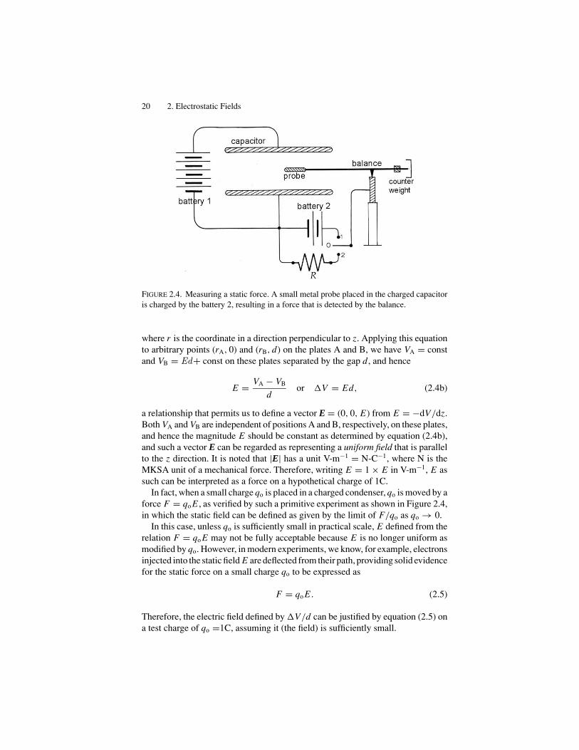
FIGURE 2.4. Measuring a static force. A small metal probe placed in the charged capacitoris charged by the battery 2, resulting in a force that is detected by the balance.
where r is the coordinate in a direction perpendicular to z. Applying this equationto arbitrary points (rA, 0) and (rB, d) on the plates A and B, we have VA = constand VB = Ed+ const on these plates separated by the gap d, and hence
E = VA − VB
dor �V = Ed, (2.4b)
a relationship that permits us to define a vector E = (0, 0, E) from E = −dV/dz.Both VA and VB are independent of positions A and B, respectively, on these plates,and hence the magnitude E should be constant as determined by equation (2.4b),and such a vector E can be regarded as representing a uniform field that is parallelto the z direction. It is noted that |E| has a unit V-m−1 = N-C−1, where N is theMKSA unit of a mechanical force. Therefore, writing E = 1 × E in V-m−1, E assuch can be interpreted as a force on a hypothetical charge of 1C.
In fact, when a small charge qo is placed in a charged condenser, qo is moved by aforce F = qo E , as verified by such a primitive experiment as shown in Figure 2.4,in which the static field can be defined as given by the limit of F/qo as qo → 0.
In this case, unless qo is sufficiently small in practical scale, E defined from therelation F = qo E may not be fully acceptable because E is no longer uniform asmodified by qo. However, in modern experiments, we know, for example, electronsinjected into the static field E are deflected from their path, providing solid evidencefor the static force on a small charge qo to be expressed as
F = qo E . (2.5)
Therefore, the electric field defined by �V/d can be justified by equation (2.5) ona test charge of qo =1C, assuming it (the field) is sufficiently small.
Uniform Electric Field in a Parallel-Plate Condenser 21
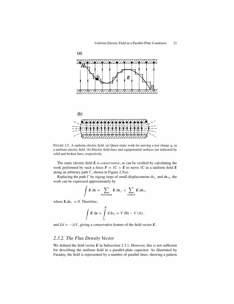
FIGURE 2.5. A uniform electric field. (a) Quasi-static work for moving a test charge qo ina uniform electric field. (b) Electric field-lines and equipotential surfaces are indicated bysolid and broken lines, respectively.
The static electric field E is conservative, as can be verified by calculating thework performed by such a force F = 1C × E to move 1C in a uniform field Ealong an arbitrary path �, shown in Figure 2.5(a).
Replacing the path � by zigzag steps of small displacements ds⊥ and ds11, thework can be expressed approximately by∫
�
E.ds =∑
horizontal
E.ds⊥ +∑
vertical
E.ds||,
where E.ds⊥ = 0. Therefore,
∫�
E.ds =B∫
A
Eds|| = V (B) − V (A) ,
and Ed = −�V , giving a conservative feature of the field vector E.
2.3.2. The Flux Density Vector
We defined the field vector E in Subsection 2.3.1. However, this is not sufficientfor describing the uniform field in a parallel-plate capacitor. As illustrated byFaraday, the field is represented by a number of parallel lines, showing a pattern

22 2. Electrostatic Fields
FIGURE 2.6. Flux of field-lines D in a uniform electric field. (a) A test capacitor Ct is insertedin the field with gap closed. (b) The gap is open in the field. (c) Ct is moved to outside ofC with the gap open.
of uniformly distributed intensities of the field. We realize that such field-lines aresignificantly related with distributed charges on conducting surfaces, although nostatic field can exist inside conducting plates. Faraday sketched such field-linesemerging from positive charges and ending at negative charges.
To express such distributed field-lines mathematically, we can utilize an in-duction effect on a conductor by an applied electric field, known as electrostaticinduction or polarization. Due essentially to mobile charges, a material placed ina condenser can be polarized by an applied electric field, exhibiting positive andnegative charges on surfaces close to the negative and positive capacitor plates,respectively. Such a polarization can also occur in an insulator, for which movablemolecules are responsible, as discussed in Section 2.5.
As shown in Figure 2.6, we indicate locations of displaced charges schematicallyby small filled and open circles for positive and negative charges, respectively. Ina parallel-plate condenser, these charges attract each other across the empty space,

Uniform Electric Field in a Parallel-Plate Condenser 23
hence residing at the closest distances. Accordingly, charges appear only on innersurfaces of the capacitor plates, whereas no charge shows up on outer surfaces.Also significant is that these charges are uniformly distributed on the parallelsurfaces, due to repulsive interactions among like charges. Consequently, the fieldin the condenser can be illustrated by parallel lines that are drawn evenly spacedto indicate the uniformity.
The uniform field in the condenser space can also be illustrated by using potentialvalues given by equation (2.4a), shown in Figure 2.5(b) by broken lines, whichrepresent a group of parallel planes at constant potentials in three dimensions,called equipotential surfaces. In fact, the field is almost uniform in the gap of theparallel-plate capacitor, except near the edge where lines are diverted as shownin the figure. Except for such diverted portions of the field, the capacitor can beidealized by uniformly distributed charge densities ± .� = ±Q/A, where A is theeffective area on the plates. In this context, it is convenient to set a rule for drawingQ lines theoretically in such a way that each line is terminated at ±1C at the ends.Accordingly, the uniform field can be expressed by a constant density of field-lines that can be written as D = Q/A. Here, it is noted that ±Q are charges on theplates, whereas the field-line density Dis a field quantity. There is no charge in theempty space, but by writing D = � we emphasize the fact that the uniform linedensity in the field is determined by the constant charge density on the plates. Withsuch flux density D, we can combine the direction from the positive to negativeplates to define the quantity D as the vector D.
To evaluate the flux density vector D in a uniform field, we perform a “thoughtexperiment” as illustrated in Figure 2.6.
Figure 2.6(a) shows a small adjustable test capacitor Ct is inserted, with thegap closed, into the uniform electric field of C . In this case, Ct is equivalent to asingle conductor, and hence polarized by the charged capacitor C , as illustrated.Here, the distributed field-lines in C are not modified from the way before insertingCt, whereas E = 0 inside Ct. It is noted that the induced charge density on Ct isequal to � i.e., it is the same density on C . Figure 2.6(b) shows that Ct is nowopen to make a gap, while the plates are kept in parallel with C . In this case,nothing significant occurs, and no field appears between the separated plates ofCt. Next, we take Ct out of C , as shown in Figure 2.6(c), where a field appearsinside Ct because polarized charges move from outside to inside surfaces. Thus,we have D = � inside Ct on moving it to outside of C , and the field pattern inC returns to the original one without Ct. In this thought experiment, we obtainD = � in Ct, regardless of where it was initially placed in the uniform field of C .The magnitude |D| at any point in the field is thus confirmed as � on the plates.Accordingly,
D = � (2.6)
expresses the flux density at all points in the uniform electric field. The MKSAunit of D is given by the same unit of surface charge density �, namely C-m−2.
Considering a static force and flux density, we have defined two vector quantitiesE and D to represent a uniform electric field. Nonetheless, these two vectors should
24 2. Electrostatic Fields
represent the same electric field, and therefore we write the relation
D = εo E, (2.7)
where the proportionality constant εo is a constant of the empty space, and whosevalue can be left for experimental evaluation. For a uniform field in a parallel-platecapacitor, we have the relations D = Q/A and E = �V/d, as expressed fromequations (2.6) and (2.4b), respectively, and hence D = εo�V/d. Accordingly,by definition, the capacity can be expressed as
Co = εoA
d(2.8)
for an empty parallel-plate capacitor. Using measured values of C , A, and d, theconstant εo can be calculated as
εo = 8.654 × 10⁻¹² F/m.
Although the physical significance is not immediately clear, the empirical value ofthe constant εo must be used for numerical calculations in static problems, usingMKSA units. In the CGS system, εo can be set equal to the dimensionless constant1, for which E and D are essentially the same quantity in a vacuum space. UsingCGS units we see that all electromagnetic phenomena are be part of the hierarchy ofmechanical space-time, although theoretical discussions are simplified by settingεo = 1.
In Section 2.2, it was shown that a charged capacitor can store energy inside.When charging up to certain amounts ±Q, the capacitor plates are characterized bypotentials VA and VB. Therefore, to transfer additional charges ±dQ to the plates,the battery should perform additional work dW = VAdQ + VB(−dQ) = �VCdQ.Since �VC = Q/C, the work W for increasing charges from 0 to ±Q can becalculated as
W = 1
C
∫ Q
0Q dQ = Q2
2C= 1
2C(�V )2.
Using (2.8) and (2.4b), W can be re-expressed by the field quantities as
W = 1
2εo E2(Ad) = 1
2DE(Ad), (2.9)
where Ad is the volume of the space between the plates. Hence, the quantity
uE = 1
2εo E2 = 1
2DE = 1
2
D2
εo(2.10)
expresses the energy density in the uniform field. Although derived for a parallel-plate capacitor, (2.9) and (2.10) can be generalized to a non-uniform static field,where the energy density uE is a function of the point r in the field. In general, thestored energy W can be calculated by
∫v
uEdv integrated over the field volume v.

Parallel and Series Connections of Capacitors 25
FIGURE 2.7. Distributing charges. (a) C1 is charged, C2 is empty, the switch S1 closed andS2 open. (b) S1, S2 are closed, and C1, C2 are both charged. (c) In the case of (a), S1 isopen and then S2 is closed. The initial charge on C1 flows partly into C2 and is distributedbetween C1 and C2.
2.4. Parallel and Series Connections of Capacitors
Combining capacitors is an elementary problem where the charging process isthermodynamically irreversible because of an energy loss during the charge dis-tribution process. In this section, we discuss parallel and series connections of twocapacitors as examples, to show that an energy loss is inevitably involved.
In Figure 2.7 are shown two capacitors C1 and C2 connected in parallel witha battery of Vemf. In Figure 2.7(a), C1 is first charged by switching S1 on, whileS2 is kept open, in which case charges are only on the plates of C1. Then, S2 isclosed with S1 on, as shown in Figure 2.7(b), thereby both capacitors C1 and C2 arecharged. In contrast, Figure 2.7(c) shows a case where the charged C1 is isolatedfrom the battery by opening S1, and C2 is uncharged if S2 is open. Closing S2,however, the charges on C1 are redistributed between the two capacitors C1 andC2.
During the process in Figure 2.7(c), it is noted that the total charge Q1 + Q2 isconstant, and the capacity of the two capacitors connected in parallel is effectivelyequivalent to a single capacity C given by
C = Q1 + Q2
Vemf= Q1
Vemf+ Q2
Vemf= C1 + C2. (2.11)
26 2. Electrostatic Fields
Equation (2.11) can be extended to parallel connections of more than two capaci-tors, for which we obtain the formula, C = ∑
iCi, where i = 1, 2, . . . .
In the process of Figure 2.7(c), the initial charges Q1 and Q2 = 0 are re-distributed as Q′
1 and Q′2 in C1 and C2, when the total charge is unchanged,
i.e., Q1 = Q′1 +Q′
2. On the other hand, it is noted that the stored ener-gies before and after redistribution are not identical, as seen from the follow-ing calculation: The initial energy stored in C1 is given by U1 = 1
2 Q21/C1,
whereas after the redistribution, the final energy stored in both capacitors isU ′ = 1
2 Q′21 /C1 + 1
2 Q′22 /C2. And, we can see easily that U1 > U ′. The differ-
ence U1 − U ′ can be attributed to heat loss of the transient current during theprocess.
For two capacitors C1 and C2 connected in series, charges on all four platesshould be in equal magnitudes but in alternate signs, i.e., +Q, −Q, +Q, −Q. Thenegative plate of C1 and the positive plate of C2 are connected together, behavinglike a single conductor, in which, obviously, E = 0. Hence, we can assign potentialsV+, − V ′, +V ′, −V−, consistent with E = 0 in the connection. Therefore, we canwrite
V+ − V− = (V+ − V ′) + (V ′ − V−),
where
V+ − V ′ = Q
C1and V ′ − V− = Q
C2.
Thus, we obtain the effective capacity C for series connection, i.e.,
1
C= 1
C1+ 1
C2, (2.12)
and the formula 1/C = �i(1/Ci) is for a series connection of more than twocapacitors.
2.5. Insulating Materials
In most practical capacitors, conducting plates are supported by insulating mate-rials to maintain a narrow gap. Therefore, the filling material should significantlymodify properties of such a capacitor. Although signified by absence of electriccurrents, most insulators exhibit polarization as induced by an electric field aris-ing from charges on the plates, and hence an insulator is often called a dielectricmaterial. Due to displaceable molecular charges, dielectric properties of fillinginsulators are essential in practical capacitors.
The electric polarization is generally a complex phenomenon, depending on theshape of material in some cases. Here, we discuss only a simple case of a dielectricslab inserted in parallel with capacitor plates of area A with a gap d, as shown inFigure 2.8.

Insulating Materials 27
FIGURE 2.8. (a) A charged empty capacitor, where the field-lines are given by D. (b) Thegap is filled with dielectric material, where there are flux D and lines of polarization P. (c)Field-lines of the vector E determined by (D − P)/ε.
To simplify the argument further, we assume that the entire space of a parallel-plate capacitor is completely filled by a slab. With a battery connected, the capacitorplates are charged not only to certain amount ±Q, but also induced charges ∓QP
appear on the surfaces of a material, being distributed at uniform densities m�P =QP = QP/A. Hence, the surface charge densities are contributed by ±� as wellas ∓�P at the boundaries, where � > �P, because of Q > QP. In this case, fluxdensity is given by � = D, but in the insulating material there are also fluxesof lines due to induced charges as determined by �P = −P . At the boundary,the free charges on the platesg cannot mix with bound charges of the insulator,but the total flux D − P inside the insulator appears as if it were originatingfrom apparent charges ±(� − �P) = ±�′ on the surfaces. We can therefore writethat
D − P = εo E, (2.12)
where E is the electric field in the material of the capacitor, for which apparentcharges ±�′ are considered to be responsible.
The induced flux P in the insulator is called the electric polarization, andconsidered as the response of the material to the applied field. A linear relation
P = � εo E (2.13)
can be applied to normal dielectrics when E is relatively weak, where the pro-portionality constant � is referred to as the electric susceptibility. In nature, spon-taneously polarized materials also exist, originating from an internal polarizingmechanism. The relation (2.13) does not hold for such materials as ferroelec-tric crystals; moreover, even in normal dielectrics the relation between P andE becomes nonlinear in a strong E field. Attributed to internal mechanisms,the solutions to these specific dielectric problems are beyond the scope of thisbook.
28 2. Electrostatic Fields
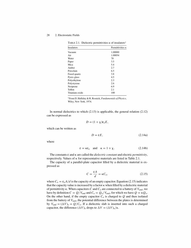
TABLE 2.1. Dielectric permittivities � of insulators∗
Insulators Permittivities �
Vacuum 1.00000Air 1.00054Water 78Paper 3.5Mica 5.4Amber 2.7Porcelain 6.5Fused quartz 3.8Pyrex glass 4.5Polyethylene 2.3Polystyrene 2.6Neoprene 6.9Teflon 2.1Titanium oxide 100
∗From D. Halliday & R. Resnick, Fundamentals of Physics,Wiley, New York, 1974.
In normal dielectrics to which (2.13) is applicable, the general relation (2.12)can be expressed as
D = (1 + � )εo E,
which can be written as
D = εE, (2.14a)
where
ε = �εo and � = 1 + � . (2.14b)
The constants ε and � are called the dielectric constant and electric permittivity,respectively. Values of � for representative materials are listed in Table 2.1.
The capacity of a parallel-plate capacitor filled by a dielectric material is ex-pressed as
C = ε A
d= �Co, (2.15)
where Co = εo A/d is the capacity of an empty capacitor. Equation (2.15) indicatesthat the capacity value is increased by a factor � when filled by a dielectric materialof permittivity �. When capacitors C and Co are connected to a battery of Vemf, wehave by definition C = Q/Vemf and Co = Qo/Vemf, for which we have Q = �Qo.On the other hand, if the empty capacitor Co is charged to Q and then isolatedfrom the battery of Vemf, the potential difference between the plates is determinedby Vemf = (�V )o = Q/Co. If a dielectric slab is inserted into such a chargedcapacitor, the difference (�V )o drops to �V = (�V )o/�.

Insulating Materials 29
Exercises
1. Calculate a change in the stored energy when a dielectric slab of permittivity �is inserted in a parallel-plate capacitor Co = εo A/d for two cases: (a) a batteryis kept connected in the circuit, and (b) the slab is inserted after Co is chargedand then isolated from the battery.
2. Obtain the expression for capacity of a parallel-plate capacitor (area A and gapd) when the space is partially filled with a dielectric slab of thickness � (< d)in parallel to the plates.
4The Laplace–Poisson Equations
4.1. The Electrostatic Potential
One of the basic properties of the electric field is the force on a small electriccharge brought in from outside the field or on a hypothetical charge of 1 C that canbe assumed as if present inside the field. On the other hand, the field as a wholeis depicted by distributed lines originating from electric charges. Represented bytwo vectors E and D, the basic laws of electrostatics are expressed in integral formas ∮
�
E.ds = 0 (3.15)
and ∮S
D.dS = 0. (3.13)
The integral in (3.15) is taken along a closed path �, whereas in (3.13) Dis integrated over a closed surface S, thereby expressing the static laws withinthe path � and surface S, which are selected for mathematical convenience. Ac-cordingly, it is also significant to formulate the laws in differential form to dealwith local properties of the field at a given position, as specified by the boundaryconditions.
First, we consider the conservative nature of the field vector E = E(r ), wherer is an arbitrary position vector in the field. Mathematically, the vanishing in-tegral in (3.15) signifies that E.ds is a perfect differential, so that we canwrite
−E.ds = dV,
with a scalar V , where the negative sign is attached for convenience. Here, thefunction V (r) is called the potential, that is, a function of a position r. The lineelement ds is taken along an arbitrary curve � for integration, but can be considered
43
44 4. The Laplace–Poisson Equations
as an arbitrary displacement dr in the field. Hence, using rectangular coordinatesr = (x, y, z), we can write that
−Ex dx − Eydy − Ezdz = ∂V
∂xdx + ∂V
∂ydy + ∂V
∂zdz,
therefore,
Ex = −∂V
∂x, Ey = −∂V
∂yEx , and Ez = −∂V
∂z. (4.1a)
The set of three differential operations (∂V /∂x , ∂V /∂y, ∂V /∂z) is a vectoroperator called the gradient, by which (4.1a) can be written as grad V or ∇V .Namely,
E = −grad V = −∇V . (4.1b)
The differential operator ∇, known as “nabla” (after a Greek word �����), isalso read “del,” and often used in place of “grad.”
It is noted that the equation V (r ) = const represents a surface in the field inthree dimensions. Characterized by a constant potential, such a surface is calledan equipotential surface. Considering two close points r and r′ on such a V =constant surface, the difference vector r − r ′ = dr indicates a tangential direction� to the surface. Therefore, from the relation V (r ) − V (r ′) ≈ grad� V . dr = 0, weobtain the relation grad� V ⊥ � . Accordingly, field-lines of vector E are alwaysperpendicular to the tangent of an equipotential surface, i.e., E ⊥ � . The staticfield can therefore be mapped by a number of equipotential surfaces of constantV , similar to altitude contours in a geographical map.
4.2. The Gauss Theorem in Differential Form
The charge Qinside in (3.13) is the total amount of the charges enclosed in a Gaussiansurface S. Taking a differential volume dv at a point r inside S, we can express thelocal charge as � (r ) dv, where � (r ) is the volume charge density at r ; and henceQinside = ∫
v
� (r )dv. The volume element dv at a point r is often written as d3r if it
is necessary to specify the point’s position in three-dimensional space. The flux isexpressed by a surface integral as in (3.13), which must be converted to a volumeintegral in order for it to be compared with the charge density � (r ) distributed inS. Such a conversion can be performed mathematically by the Gauss theorem.
For simplicity, we use here rectangular coordinates to derive the Gauss theorem,as shown in Fig. 4.1(a).
We consider a volume element dv = dxdydz in cube shape, where three pairsof rectangular planes of area dydz, dzdx, and dxdy are facing along the x , y,
and z directions, respectively, constituting a closed cubical surface dS coveringthe volume dv. For such a small volume, the flux on the left side of (3.13) can be

The Gauss Theorem in Differential Form 45
FIGURE 4.1. (a) A differential volume element in rectangular coordinates. (b) An elementin curvilinear coordinates (u1, u2, u3).
specially expressed as∑dS
D.dS = −Dx dSx + Dx+dx dSx − DydSy + Dy+dydSy − DzdSz + Dz+dzdSz
= (Dx+dx − Dx ) dydz + (Dy+dy − Dy
)dzdx + (Dz+dz − Dz) dxdy
=(
∂ Dx
∂x+ ∂ Dy
∂y+ ∂ Dz
∂z
)dxdydz,
whereas the charge on the right side of (3.13) is given by
Qinside = � (x, y, z) dxdydz.
Therefore, the flux law (3.13) can be written as
∂ Dx
∂x+ ∂ Dy
∂y+ ∂ Dz
∂z= � (x, y, z) . (4.2a)
Using the vector differential operator ∇, the left hand side expression in (4.2a)can be expressed by the scalar product of ∇. D, called the divergence of D, andtherefore we obtain
∇.D(r ) = � (r ) (4.2b)
or
div D(r ) = � (r ). (4.2c)
If the space is empty or filled with a uniform dielectric medium, we have arelation D = εo E or D = εE, respectively, and (4.2b) and (4.2c) can be writtenfor E as
∇.E = divE = � (r )/εo or � (r )/ε. (4.2d)
In (4.2d), the expressions in empty and filled spaces are identical, except for thedielectric constants, and hence it is sufficient to discuss the equation for εo for an
46 4. The Laplace–Poisson Equations
empty field. The field in normal media can be described sufficiently by one of thesevectors D or E. In contrast, the potential function V (r ) derived from (4.1a and b) isa scalar quantity, making mathematical analysis significantly simpler. Combining(4.1a) and (4.1b) with (4.2d), we can write the equation for the potential as
−∇.∇V (r ) = −div.grad V (r ) = � (r )
ε,
where
∇.∇ = div.grad = ∂2
∂x2+ ∂2
∂y2+ ∂2
∂z2
is a scalar operator called a Laplacian, and often expressed by ∇.∇ = ∇2 = Δ.The equation for V (r ) is an inhomogeneous differential equation when � (r ) �= 0,
but becomes a homogeneous equation if � (r ) = 0. In the former case
∇2V (r ) = −� (r )
ε(4.3)
is called the Poisson equation, whereas the homogeneous equation in the latter,i.e.,
∇2V (r ) = 0, (4.4)
is the Laplace equation. Representing the basic laws of electrostatics, these equa-tions are to be solved for the potential V (r ), subject to given boundary conditions.
4.3. Curvilinear Coordinates (1)
For electrostatic problems in most practical cases, symmetry of boundaries playsa significant role in obtaining solutions of the Laplace equation. In Section 4.2rectangular coordinates were used for simplicity; however, for practical problemsbasic equations may have to be expressed in polar, cylindrical, or other coordinates,depending on the symmetry of a problem.
Polar and cylindrical coordinates are specific curvilinear coordinates that cangenerally be written as u1, u2, and u3. Nevertheless, these coordinates are alsofunctions of rectangular coordinates x, y, and z; a point P(x, y, z) in space canalso be specified by (u1, u2, u3). An important feature of these curvilinear systemsis that basic coordinate surfaces (0, u2, u3), (u1, 0, u3) and (u1, u2, 0) are mutuallyorthogonal, and a differential displacement dr can be expressed by the metric
dr2 = h21du2
1 + h22du2
2 + h23du2
3, (4.5)
representing the orthogonal space. In general, the coordinate transformation isspecified by the metric dr2 = �gijuiuj expressed with coefficients gij = hihj,which constitute a metric tensor (gij).
Judging from (4.5), in the orthogonal space components of dr are given bycomponents h1du1, h2du2, and h3du3, where h1, h2, and h3 can be considered
Curvilinear Coordinates (1) 47
factors for adjusting coordinates u1, u2, and u3 to linear dimensions. The gradientof a scalar function V can therefore be expressed by components
E1 = − 1
h1
∂V
∂u1, E2 = − 1
h2
∂V
∂u2and E3 = − 1
h3
∂V
∂u3. (4.6)
For example, with rectangular coordinates (x, y, z) equation (4.5) for the metriccan be expressed as
dr2 = dx2 + dy2 + dz2,
where
u1 = x, u2 = y, u3 = z
and
h1 = h2 = h3 = 1.
Hence, the gradient vector is given by (4.1a).For polar coordinates (r, �, ), on the other hand, we have
dr2 = dr2 + r2d�2 + r2 sin2 � d2,
for which
u1 = r, u2 = �, u3 =
and
h1 = 1, h2 = r, h3 = r sin �.
In this case, from (4.6) the vector E has components
Er = −∂V
∂r, E� = −1
r
∂V
∂�, and E = − 1
r sin �
∂V
∂. (4.7)
Similarly, with cylindrical coordinates (� , �, z) we have
dr2 = d� 2 + � 2d�2 + dz2,
for which
u1 = � , u2 = �, u3 = z
and
h1 = 1, h2 = � , h3 = 1.
The vector E is then expressed by
E� = −∂V
∂�, E� = − 1
�
∂V
∂�and Ez = −∂V
∂z. (4.8)
When converting a surface integral∫S
D.dS into a volume integral, the
volume element needs to be written by curvilinear coordinates as dv =(h1du1)(h2du2)(h3du3). Similar to a volume element dv = dxdydz in rectangular

48 4. The Laplace–Poisson Equations
coordinates, the cube-like elemental volume dv has three pairs of surfaces—(dS1, dS′
1), (dS2, dS′2), and (dS3, dS′
3)—that are perpendicular to the u1, u2, and u3
lines, respectively, as shown in Fig. 4.1(b).In this case, the flux d� determined by dS can be calculated as
d� = �D.dS
= (−D1dS1 + D′1dS′
1) + (−D2dS2 + D′2dS′
2) + (−D3dS3 + D′3dS′
3), (4.9)
where
dS′1 = h′
2h′3du2du3
=(
h2 + ∂h2
∂u1du1
) (h3 + ∂h3
∂u1
)du2du3, D′
1 = D1 + ∂ D1
∂u1du1, etc.
Therefore, we can write
D′1dS′
1 = D1h2h3du2du3 +(
∂ D1
∂u1h2h3 + D1
∂h2
∂u1h3 + D1h2
∂h3
∂u1
)du1du2du3
= D1dS1 + ∂ (D1h2h3)
∂u1du1du2du3,
from which we derive
D′1dS′
1 − D1dS1 = 1
h1h2h3
∂ (D1h2h3)
∂u1dv.
Similarly,
D′2dS′
2 − D2dS2 = 1
h1h2h3
∂ (D2h3h1)
∂u2dv
and
D′3dS′
3 − D3dS3 = 1
h1h2h3
∂ (D3h1h2)
∂u3dv.
Accordingly, we arrive at the expression
d� = 1
h1h2h3
{∂ (D1h2h3)
∂u1+ ∂ (D2h3h1)
∂u2+ ∂ (D3h1h2)
∂u3
}dv = (div D) dv.
Therefore, the total flux integrated over a closed surface S can be expressed by∮S
D.dS =∫v
div D dv, (4.10)
where
div D = 1
h1h2h3
{∂ (D1h2h3)
∂u1+ ∂ (D2h3h1)
∂u2+ ∂ (D3h1h2)
∂u3
}. (4.11)
Equation (4.10) is the conversion formula between surface and volume inte-grals, which is known as the Gauss theorem. Equation (4.10) gives the generalexpression of div D in curvilinear coordinates u1, u2, and u3. Using (4.10), div

The Laplace–Poisson Equations 49
D can be expressed in representative curvilinear coordinates. First, in rectangularcoordinates as
div D = ∂ Dx
∂x+ ∂ Dy
∂y+ ∂ Dz
∂z. (4.11a)
In polar coordinates as
div D = 1
r2 sin �
{∂
(r2 sin �Dr
)∂r
+ ∂ (r sin �D�)
∂�+ ∂
(r D
)∂
}. (4.11b)
In cylindrical coordinates as
div D = 1
�
∂(� D�
)∂�
+ 1
�
∂ D�
∂�+ ∂ Dz
∂z. (4.11c)
The Laplacian operator can also be expressed as
∇2 = ∂2
∂x2+ ∂2
∂y2+ ∂2
∂z2, (4.12a)
∇2 = 1
r2
∂
∂r
(r2 ∂
∂r
)+ 1
r2 sin �
∂
∂�
(sin �
∂
∂�
)+ 1
r2 sin2
∂2
∂2, (4.12b)
∇2 = 1
�
∂
∂�
(�
∂
∂�
)+ 1
�2
∂2
∂�2+ ∂2
∂z2, (4.12c)
for rectangular, polar, and cylindrical systems, respectively.
4.4. The Laplace–Poisson Equations
A basic mathematical problem in electrostatics is to solve the Laplace equationfor the potential function when a charge distribution is specified on the boundary.If there are charges on conducting boundaries and in the field we have to dealwith the Poisson equation at these charges’ locations. For a complete solution ofa static problem, both these equations are often required under given boundaryconditions. Mathematically, such a problem can be discussed with the Green’sfunction method, which is generally applicable to other boundary problems thanthose encountered in electrostatics. In this section, the Green’s function methodis outlined so we may discuss its mathematical consequences for static problems,although some results are inferable with respect to physical ideas.
4.4.1. Boundary Conditions
In Section 3.4 static boundary conditions were discussed using the field vectors Eand D. For a conducting boundary the conditions are generally specified by (3.16)as
Et = 0 and Dn = ,
50 4. The Laplace–Poisson Equations
which may alternatively be expressed with the potential function in the field as
(V )S = 0 and − εo
(∂V
∂n
)S
= , (4.13)
where the suffix S indicates the specific value on the boundary surface.For dielectric boundaries, the conditions (3.17) can be expressed as
(∂V
∂t
)1S
=(
∂V
∂t
)2S
and ε1
(∂V
∂n
)1S
= ε2
(∂V
∂n
)2S
, (4.14)
which can also be specified by continuities of (V )S and ε(∂V /∂n)S across theboundary. On a dielectric boundary, due to different ε1 and ε2, (∂V /∂n)S cannot becontinuous in general; however the condition can be specified by V and ∂V /∂n ata point on the surface S. However, such a dielectric boundary may not necessarilybe a field boundary a specific if we consider that all the boundary points are phys-ically characterized by a common property. As discussed in Section 3.4, a planardielectric boundary in a uniform electric field is regarded as an equipotential onlyif it is parallel with the plates, which is, however, example. Nevertheless, a practi-cal field is confined to an empty or material-filled space with conducting boundsS specified by continuous (V )S and discontinuous ε(∂V /∂n)S . Known as Dirich-let’s conditions, such boundaries are one type considered in the mathematicaltheory.
Although primarily “closed,” practical boundary surface S may have an “open”area S′ as well. If a small hole exists on a plate of a capacitor, for exam-ple, the field can no longer be uniform in the vicinity of the hole, from wheresome field-lines may “leak out.” Such a hole area S′ in an empty capacitorshould be considered as distinct from closed area S, the former being physi-cally characterized by the absence of surface charge. On S′, inside and outsidefields are connected by the same medium of εo, where (∂V /∂n)S′ is continu-ous and expressed as continuous Dn across the area S′. In a general theory ofboundary problems, such a boundary as specified by continuous (∂V /∂n)S′ iscalled Neumann’s boundary. Although somewhat specific from a physical view-point, a general boundary is regarded as consisting of such surfaces as S and S′,on which Dirichlet’s and Neumann’s conditions can be imposed, respectively.In Subsection 4.4.3, the boundary problem for the Laplace-Poisson equationsis discussed with Green’s function, where boundary surfaces S and S′ of bothtypes are considered. In the next subsection, we pay attention to the uniquenesstheorem of the potential prior to discussing the method of Green’s function inSubsection 4.4.3.
4.4.2. Uniqueness Theorem
Static potentials given by solutions of the Laplace–Poisson equations are uniquelydetermined with the boundary conditions on S and S′ characterized by continuous
The Laplace–Poisson Equations 51
(V )S and (∂V /∂n)S′ , respectively, constituting a statement known as the uniquenesstheorem. Here the theorem is proved, thereby assuring that the Laplace-Poissonequations have unique solutions in a given field.
Assuming that two different potentials V and V ’ obey the same Laplace−Poisson equations, we can prove that the difference function = V – V ’ can takeno values other than zero at all given points. For that purpose we consider a trialvector function ∇, which is then subjected to the Gauss theorem. For such afunction we can write∫
v
div (∇) dv =∫
S+S′
∇.d(S + S′) =
∫S+S′
∂
∂nd
(S + S′) = 0,
because = 0 on S and ∂/∂n = 0 on S′. On the other hand,
div(∇) = div(∇) + (∇)2 = (∇)2,
because of the identity div(∇) ≡ 0, and hence∫v
(∇)2 dv = 0.
Noting that the integrand (∇)2 can be either positive or zero, this integralbecomes zero only when ∇ = 0, or = onstant. Therefore, V − V ′ is physicallyinsignificant constant, assuring that the potential V (r ) can always be unique at agiven position r.
4.4.3. Green’s Function Method
In this subsection we discuss a general problem for the potential V (r ) in a field ofdistributed charges on the boundary surface S. We consider that the distribution canprimarily be specified by a volume density � (r ′) at a point r ′ in the surface region,although a surface density can be redefined as surface charges on a mathematicalboundary. By considering � (r ′), the potential should obey the Poisson equation
∇2V (r ′) = −�(r ′)
εo. (4.15)
Assuming highly localized charges, the density may be expressed as � (r − r ′) =��(r − r ′) using a delta function �(r − r ′) to specify a finite � located only atr = r ′, whereas 0 at any other point r �= r ′.
We define a function G(r − r ′) that satisfies the equation
∇2G(r − r ′) = −�(r − r ′)εo
(4.16)
and is called the Green function. The equation (4.16) is the Laplace equation atall points r other than r ′, but it is the Poison equation at r = r ′. Considering � as
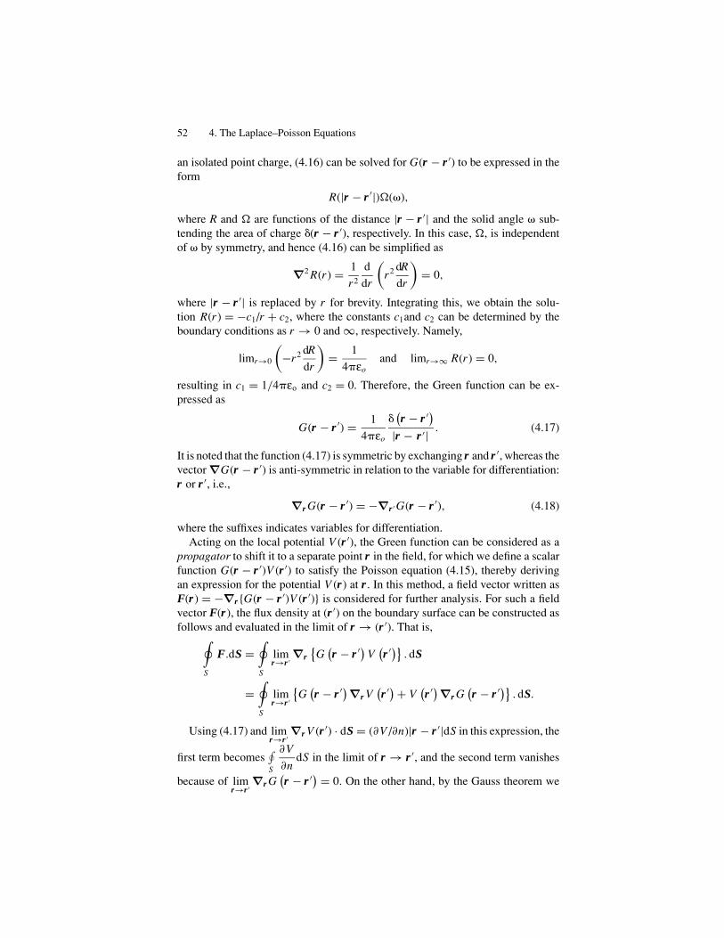
52 4. The Laplace–Poisson Equations
an isolated point charge, (4.16) can be solved for G(r − r ′) to be expressed in theform
R(|r − r ′|)�(�),
where R and � are functions of the distance |r − r ′| and the solid angle � sub-tending the area of charge �(r − r ′), respectively. In this case, �, is independentof � by symmetry, and hence (4.16) can be simplified as
∇2 R(r ) = 1
r2
d
dr
(r2 dR
dr
)= 0,
where |r − r ′| is replaced by r for brevity. Integrating this, we obtain the solu-tion R(r ) = −c1/r + c2, where the constants c1and c2 can be determined by theboundary conditions as r → 0 and ∞, respectively. Namely,
limr→0
(−r2 dR
dr
)= 1
4 εoand limr→∞ R(r ) = 0,
resulting in c1 = 1/4 εo and c2 = 0. Therefore, the Green function can be ex-pressed as
G(r − r ′) = 1
4 εo
�(r − r ′)
|r − r ′| . (4.17)
It is noted that the function (4.17) is symmetric by exchanging r and r ′, whereas thevector ∇G(r − r ′) is anti-symmetric in relation to the variable for differentiation:r or r ′, i.e.,
∇r G(r − r ′) = −∇r ′ G(r − r ′), (4.18)
where the suffixes indicates variables for differentiation.Acting on the local potential V (r ′), the Green function can be considered as a
propagator to shift it to a separate point r in the field, for which we define a scalarfunction G(r − r ′)V (r ′) to satisfy the Poisson equation (4.15), thereby derivingan expression for the potential V (r ) at r . In this method, a field vector written asF(r ) = −∇r {G(r − r ′)V (r ′)} is considered for further analysis. For such a fieldvector F(r ), the flux density at (r ′) on the boundary surface can be constructed asfollows and evaluated in the limit of r → (r ′). That is,∮
S
F.dS =∮S
limr→r ′
∇r{G
(r − r ′) V
(r ′)} . dS
=∮S
limr→r ′
{G
(r − r ′) ∇r V
(r ′) + V
(r ′) ∇r G
(r − r ′)} . dS.
Using (4.17) and limr→r ′
∇r V (r ′) · dS = (∂V /∂n)|r − r ′|dS in this expression, the
first term becomes∮S
∂V
∂ndS in the limit of r → r ′, and the second term vanishes
because of limr→r ′
∇r G(r − r ′) = 0. On the other hand, by the Gauss theorem we

Simple Examples 53
have ∮S
F.dS =∫v
(∇r .F) dv =∫v
∇r .∇r{G
(r − r ′) V
(r ′)} dv
=∫v
∇r ′ .∇r ′{G
(r − r ′) V
(r ′)}dv
=∫v
V(r ′) ∇2
r ′ G(r − r ′) dv +
∫v
G(r − r ′) ∇2
r ′ V(r ′) dv
= −∫v
G(r − r ′) �
(r ′)
εodv −
∫v
V(r ′) �
(r − r ′)εo
dv,
in which the second term of the last expression can be simplified as V (r )/εo. Here,∮S
F · dS should be equal to εo
∮S
∂V
∂ndS, and we finally obtain
V (r ) =∫v
�(r ′) G
(r − r ′) dv + εo
(∂V
∂n
)S
,
= 1
4 εo
∫v′
�(r ′) �
(r − r ′)∣∣r − r ′∣∣ dv′ + εo
(∂V
∂n
)S
. (4.19)
It is noted that the integral in (4.19) is to be carried out for the volume ofdistributed charges v′, and hence the first term expresses a Coulomb potential dueto the total charge that looks like a point charge at a distant point r r ′. Also,we can apply formula (4.19) directly to individual charges in a group of charges,which can be added to obtain the total potential.
4.5. Simple Examples
In this section we discuss simple applications of the Laplace–Poisson equationsand the Coulomb potential in fields of high symmetry, applications that require onlyelementary mathematical analysis. Problems for advanced mathematical analysiswill be discussed in Chapter 5.
Example 1. A Long Cylindrical Capacitor.The electric field and potential in a cylindrical capacitor were already discussed
in Section 3.4. In this example the same problem is discussed with the Laplaceequation as the mathematical exercise. The charge density on the conductor isexpressed by a given charge per length, i.e., � = Q/ l, where the field is radialand perpendicular to the conductor and expressed as a function of radius � onlyif the length is sufficiently long, where � = a and b are radii of inner and outerconducting surfaces. By virtue of cylindrical symmetry, the coordinates � and z

54 4. The Laplace–Poisson Equations
FIGURE 4.2. A circular parallel-plate con-denser. The point P is specified by cylin-drical coordinates (� , �, z). The origin Ois set at the center.
are not necessary, and hence from (4.12c) the Laplace equation can be written as
1
�
d
d�
(�
dV
d�
)= 0.
This can be integrated as
dV
d�= c
�and V = c ln � + c′ for a ≤ � ≤ b.
The integration constant c can be determined by the boundary condition on theconductor surface � = a, that is, (D� )�=a = a (the surface charge density). Here,a = �/2 a, and from the relations −εo(dV/d� )�=a = a , and −εo(dV/d� )�=b =b we obtain
c = �/2 εo.
The other constant, c′, can be obtained from the relation (V )�=a = c ln a + c′,but is left undetermined as insignificant because only the potential difference isphysically meaningful. Hence,
V (� ) = �
2 εoln � + c and E� g − ∂V
∂�= �
2 εo�.
Exercise. Using the Laplace equation, obtain the expressions for the potential andelectric field of radii a and b, respectively, in a spherical capacitor.
Example 2. A Parallel-Plate Capacitor of Circular Plates.In a parallel-plate capacitor of gap d and circular area A of radius R, i.e.,
A = R2, we consider R not to be significantly larger than d. However, note thatthe capacitor is symmetric around the z-axis, as shown in Fig. 4.2, and hence theLaplace equation can be expressed with cylindrical coordinates � , �, and z, wherethe angle � is unnecessary for circular symmetry. That is,
�∂
∂�
(�
∂V
∂�
)+ � 2 ∂2V
∂�2= 0.

The Coulomb Potential 55
Assuming that V (� , z) = P(� )Z (z), the equation can be written as a sum oftwo separated terms of � only and of z only, that is,
1
� P
d
d�
(�
dP
d�
)+ 1
Z
d2 Z
dz2= 0.
Therefore, by introducing a constant �2, we can separate the equation into twoequations
1
Z
(d2 Z
dz2
)= �2 (i)
and1
� P
d
d�
(�
dP
d�
)= −�2, (ii)
Rewriting (ii), we obtain
d2 P
d� 2+ 1
�
dP
d�+ �2 P = 0,
that is, the Bessel equation, whose solution is expressed by
P (� ) = P (0) Jo (�� ) .
Equation (i) has a solution generally given by exp(±�z), but we take their linearcombination to write
Z (z) = Z (0) sinh(�z)
to satisfy the boundary conditions on the plates at z = ±1
2d. Denoting the potential
difference between the plates by �V , the solution of the Laplace equation can thenbe expressed as
V (� , z) = 1
2�V Jo(�� ) sinh(�z), where �V = 4P(0)Z (0).
The boundary conditions at z = ±1
2d are
−εo
(∂(� , z)
∂z
)z=± 1
2 d
= ± εo
2��V cosh
(1
2�d
)Jo(�� ) = ±(� ),
which are not constant as in a capacitor of A = ∞, but approaching constant valuesas � → 0. It is noted that � and z become independent in this limit.
4.6. The Coulomb Potential
Examples for the Coulomb potential (4.19) are discussed in this section using thepoint-charge model to calculate for static fields. Although only mathematicallyjustifiable, a point charge can be considered as a solution (4.19) of the Laplaceequation, which is used as a classical model to represent charged particles.
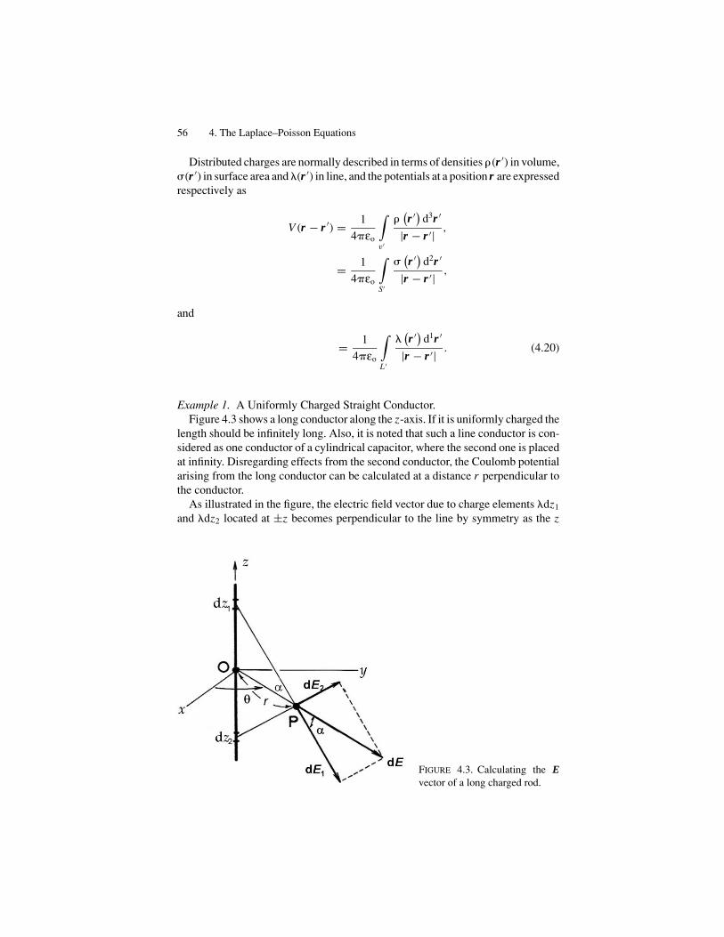
56 4. The Laplace–Poisson Equations
Distributed charges are normally described in terms of densities � (r ′) in volume,(r ′) in surface area and �(r ′) in line, and the potentials at a position r are expressedrespectively as
V (r − r ′) = 1
4 εo
∫v′
�(r ′) d3r ′
|r − r ′| ,
= 1
4 εo
∫S′
(r ′) d2r ′
|r − r ′| ,
and
= 1
4 εo
∫L ′
�(r ′) d1r ′
|r − r ′| . (4.20)
Example 1. A Uniformly Charged Straight Conductor.Figure 4.3 shows a long conductor along the z-axis. If it is uniformly charged the
length should be infinitely long. Also, it is noted that such a line conductor is con-sidered as one conductor of a cylindrical capacitor, where the second one is placedat infinity. Disregarding effects from the second conductor, the Coulomb potentialarising from the long conductor can be calculated at a distance r perpendicular tothe conductor.
As illustrated in the figure, the electric field vector due to charge elements �dz1
and �dz2 located at ±z becomes perpendicular to the line by symmetry as the z
FIGURE 4.3. Calculating the Evector of a long charged rod.

The Coulomb Potential 57
FIGURE 4.4. Calculating the E vector of a charged plate of infinite area.
components of dE1 and dE2 are cancelled. Therefore,
|dE| = 1
4 εo
∞∫0
2� dz
z2 + r2cos �, where cos � = r√
z2 + r2.
Hence, we obtain
|E| = Er = �
2 εo
∞∫0
rdz(z2 + r2
) 32
= �
2 εor,
and the logarithmic potential
V (r ) = �
2 εoln r + const.
Example 2. A Charged Surface of a Conductor.Figure 4.4 shows a flat conducting surface, where the charge distribution is
considered to be uniform. However, this assumption is valid only if the surfaceextends to infinity. Besides, E = 0 inside the conductor, as characterized by aconstant V that can be equal to 0 if the area is infinitely large. In this case, the fieldvector is strictly perpendicular to the surface because of the symmetry and of aconstant magnitude as derived by the Gauss theorem.
As illustrated in the figure, at a point P(0, 0, h) we consider all surface chargesin a ring area between circles of radii � and � + d� , and notice that field elementsdE1 and dE2 due to differential charges on areas �d�d� at � and � + have hor-izontal components that are cancelled by symmetry and signified only by vertical
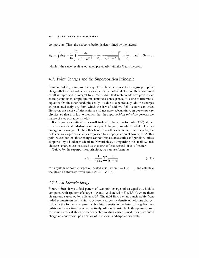
58 4. The Laplace–Poisson Equations
components. Thus, the net contribution is determined by the integral
Eh =∫S
dEh =
εo
∞∫0
rdr(r2 + h2
) 32
=
εo
∣∣∣∣− h√r2 + h2
∣∣∣∣∞
0
=
εo, and Dh = ,
which is the same result as obtained previously with the Gauss theorem.
4.7. Point Charges and the Superposition Principle
Equations (4.20) permit us to interpret distributed charges at r ′ as a group of pointcharges that are individually responsible for the potential at r , and their combinedresult is expressed in integral form. We realize that such an additive property ofstatic potentials is simply the mathematical consequence of a linear differentialequation. On the other hand, physically it is due to algebraically additive chargesas postulated early on, from which the law of additive field vectors can arise.However, the nature of electricity is still not quite substantiated in contemporaryphysics, so that it is fair to mention that the superposition principle governs thenature of electromagnetic fields.
If charges are confined to a small isolated sphere, the formula (4.20) allowsus to consider it at a distant point as a point charge from which radial field-linesemerge or converge. On the other hand, if another charge is present nearby, thefield can no longer be radial, as expressed by a superposition of two fields. At thispoint we realize that those charges cannot form a stable static configuration, unlesssupported by a hidden mechanism. Nevertheless, disregarding the stability, suchclustered charges are discussed as an exercise for electrical states of matter.
Guided by the superposition principle, we can use formulas
V (r ) = 1
4 εo
∑i
qi
|r − r i| (4.21)
for a system of point charges qi located at r i, where i = 1, 2, . . . , and calculatethe electric field vector with and E(r ) = −∇V (r ).
4.7.1. An Electric Image
Figure 4.5(a) shows a field pattern of two point charges of an equal q, which iscompared with a pattern of charges +q and −q sketched in Fig. 4.5(b), where thesecharges are separated by a distance 2h. The field-lines deviate considerably fromradial symmetry in their vicinity; between charges the density of field-line chargesis low in the former, compared with a high density in the latter, arising from re-pulsive and attractive forces, respectively. Although unstable, both represent casesfor some electrical states of matter each providing a useful model for distributedcharge on conductors, polarization of insulators, and dipolar molecules.
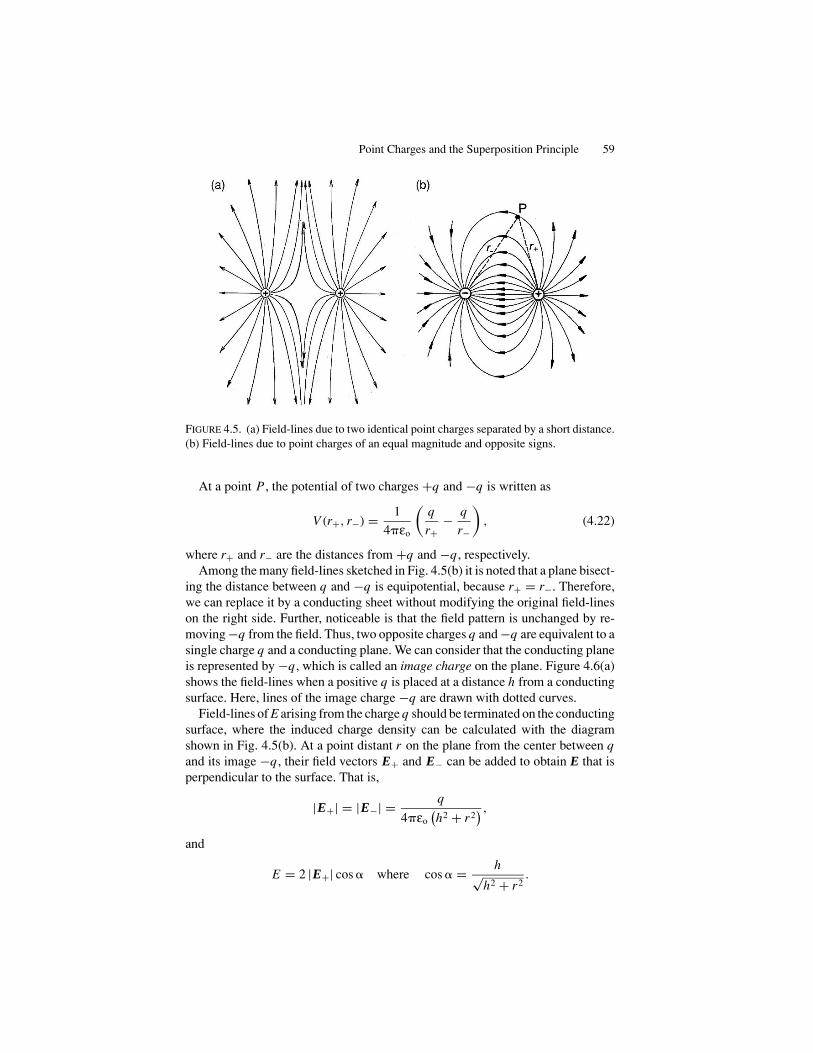
Point Charges and the Superposition Principle 59
FIGURE 4.5. (a) Field-lines due to two identical point charges separated by a short distance.(b) Field-lines due to point charges of an equal magnitude and opposite signs.
At a point P , the potential of two charges +q and −q is written as
V (r+, r−) = 1
4 εo
(q
r+− q
r−
), (4.22)
where r+ and r− are the distances from +q and −q, respectively.Among the many field-lines sketched in Fig. 4.5(b) it is noted that a plane bisect-
ing the distance between q and −q is equipotential, because r+ = r−. Therefore,we can replace it by a conducting sheet without modifying the original field-lineson the right side. Further, noticeable is that the field pattern is unchanged by re-moving −q from the field. Thus, two opposite charges q and −q are equivalent to asingle charge q and a conducting plane. We can consider that the conducting planeis represented by −q , which is called an image charge on the plane. Figure 4.6(a)shows the field-lines when a positive q is placed at a distance h from a conductingsurface. Here, lines of the image charge −q are drawn with dotted curves.
Field-lines of E arising from the charge q should be terminated on the conductingsurface, where the induced charge density can be calculated with the diagramshown in Fig. 4.5(b). At a point distant r on the plane from the center between qand its image −q , their field vectors E+ and E− can be added to obtain E that isperpendicular to the surface. That is,
|E+| = |E−| = q
4 εo(h2 + r2
) ,
and
E = 2 |E+| cos � where cos � = h√h2 + r2
.

60 4. The Laplace–Poisson Equations
FIGURE 4.6. (a) A point charge q and its electric image −q on infinite conducting plane.(b) Calculating the image force.
This perpendicular field should be related to an induced charge density, whichcan be written as
− (r ) = −εo E (r ) = − qh
2 (h2 + r2
) 32
,
indicating maximum at r = 0. The total amount of induced charges on the surfacecan be calculated by integrating −(r ) over the entire area, that is,
−∞∫
0
(r ) rdr
2 ∫0
d� = qh
2
∞∫0
rdr(h2 + r2
) 32
× 2 = − qh
2
1
h2 = −q,
which is exactly equal to the image charge. Owing to the negative sign of the imagecharge or total induced charge, the charge q is attracted by the conducting plate.The force is expressed as the Coulomb force between point charges q and −q andcalled an image force. That is,
F = − 1
4 εo
q2
(2h)2 . (4.23)
4.7.2. Electric Dipole Moment
Asymmetric molecules are often represented electrically by a pair of charges qand −q that are separated by a small finite distance l. Such a separation l is sosmall in size that the pair of charges appears as if neutral as observed at a verydistant point. However, at a closer distance, the pair of charges exhibits explicitfield-lines, called a dipolar field. Such a distance r for a predominantly dipolar

Point Charges and the Superposition Principle 61
FIGURE 4.7. Calculation of the dipolar po-tential at a distant point P(r, �, ).
field is significantly larger than l, where the pair of charges is characterized by theproduct ql called an electric dipole.
Figure 4.7 shows such a model of a dipole located at the origin of a coordinatesystem, and along the z axis. It is usually free to rotate, and hence representedconveniently by a vector quantity defined by
p = ql, (4.24)
where the vector l signifies the direction from −q to q, and the vector p is referredto as the dipole moment. The MKSA unit of a dipole moment is C-m, whichhowever is too large for molecular dipoles of the order of 10−29 C-m. In molecularphysics, we traditionally use the unit called “Debye” defined as equal to 10−18
esu-cm. Typical examples are p = 0.12 Debye for CO, and 1.86 Debye for H2O.The dipole potential can be obtained with a model in Fig. 4.5(b) by considering
2h = l. The potential can be calculated from (4.22) approximately for r l. Notedthat
r2± = r2 +
(l
2
)2
∓ 2r
(l
2
)cos �,
we expand1
r±with respect to a small
l
r, and derive
1
r±= 1
r
√1 +
(l
r
)2
∓ l
rcos �
≈ 1
r
(1 ± l
2rcos � + · · ·
)for r l.
Therefore, the potential can be approximately expressed as
V (r+, r−) ≈ 1
4 εo
ql
r2cos � = 1
4 εo
p cos �
r2.

62 4. The Laplace–Poisson Equations
FIGURE 4.8. (a) An electric dipole moment in a uniform electric field E. (b) Dipole-dipoleinteraction.
Since we defined the dipole moment as a vector, the dipole potential can be writtenas
V1(r ) = 1
4 εo
p. rr3
, (4.25)
where the index 1 is attached to V1(r ) as related to the order in the series expansionof potentials, as the potential will be expressed in higher approximation in laterdiscussions.
If an electric dipole p can be in rotational motion like a molecular dipole, externalfield E exerts a torque. Figure 4.8(a) shows such a dipole in a uniform field, wherea couple of forces +qE and −qE is responsible for rotating the dipole moment.Accordingly, the dipole has a potential energy for rotation
U = −p.E = −pE cos� (4.26a)
as related to the torque
� = p × E where |� | = pE sin�. (4.26b)
Here � is the angle between the vectors p and E.If E is not uniform over the dipole moment along a direction x , we need to
consider a force related to the field gradient in addition to the torque given by(4.26b). Such a force is responsible for translational motion of the dipole. If thefield E varies as a function of position x , a field gradient arises from the differencebetween fields at q and −q, i.e.,
E(x + dx) − E(x) = (∂ E/∂x) dx,
where dx = lcos�, and therefore the net force is given by
F = q∂ E
∂xl cos � = p cos �
∂ E
∂x. (4.26c)
Point Charges and the Superposition Principle 63
4.7.3. The Dipole-Dipole Interaction
In dielectric materials, polar molecules can be represented by their dipole moments.In this case, the mutual interaction energy arises from dipole-dipole interactions.Considering two dipole moments p1 and p2 that can be rotated at fixed positionsas shown in Fig. 4.8(b), the interaction potential can be calculated for a givendistance. The distance between p1 and p2 can be expressed as a vector r, althoughthe direction is not significant for the mutual interaction energy. Nevertheless,directions of interacting dipole moments are significantly related to their distancefrom one another. On the other hand, the interaction energy should be unchangedby inverting r to −r , as consistent with Newton’s action-reaction principle.
The interaction energy can be calculated for p1 to be in the dipole field of p2 orfor p2 in the field of p1. In either case, we combine (4.25) and (4.26a) as derivedin the following. The electric field originating from p2 at the position of p1 can beexpressed as
E12 = − 1
4 εo∇1
p2. rr3
= 3(
p2. r)
r − p2r2
4 εor5,
and hence p1 has an energy
U12 = −p1. E12 = 1
4 εo
[(p1. p2) r2 − 3 (p1. r ) (p2. r )
r5
]. (4.27)
Similarly, we obtain the expression for U21 = − p2. E21 that is identical to(4.27). Equation (4.27) is the formula for a dipole-dipole interaction.
3The Gauss Theorem
3.1. A Spherical Capacitor
Spherical and cylindrical capacitors are important devices in practical applicationsas well as for simple analysis of a static electric field. In these capacitors, field-linescan be visualized precisely as radial, thereby the model of a point and line chargecan be established.
Figure 3.1 shows a sectional view of two concentric conducting spherical shellsconnected to a battery of Vemf. In this case, charges ±Q are distributed uniformlyover the surfaces facing each other, as illustrated in the figure. Denoting the radiiof these surfaces by a and b where a < b, the surface charge densities are given by�a = Q/4�a2 and −�b = −Q/4�b2, respectively. Assuming Q > 0, field-linesstart from positive charges on the outer spherical surface of radius a, and endat negative charges on the inner spherical surface of radius b. Inside conductingmaterials, the field E should be zero in a static condition, and in the outsidespace of the outer conductor there is no field, since no charges appear on theoutermost surface. These conducting spheres can be signified by unique electricalpotentials Va and Vb, where Va > Vb if Q > 0, and all concentric spheres of radiusr are equipotential in the range of a ≤ r ≤ b. According to the drawing rule forfield-lines given in Section 2.3.2, the number of lines should, theoretically, beequal to Q, and expressed by Q = �a(4�a2) = �b(4�b2). For an equipotentialsurface with an arbitrary radius r , the flux density Dr can be calculated from theintegral ∮
S
Dr dSr = Dr (4�r2) = Q,
where dSr is the surface element on a sphere of radius r . Because of the sym-metry, field-lines are all radial, and hence Dr represents the radial compo-nent of the flux density vector D. Therefore, for a spherical capacitor, we canwrite
Dr = Q
4�r2and Er = Q
4�εor2. (3.1)
30
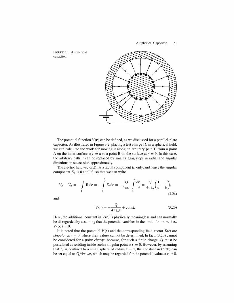
A Spherical Capacitor 31
FIGURE 3.1. A spherical
capacitor.
The potential function V (r ) can be defined, as we discussed for a parallel-platecapacitor. As illustrated in Figure 3.2, placing a test charge 1C in a spherical field,we can calculate the work for moving it along an arbitrary path � from a pointA on the inner surface at r = a to a point B on the surface at r = b. In this case,the arbitrary path � can be replaced by small zigzag steps in radial and angulardirections in succession approximately.
The electric field vector E has a radial component Er only, and hence the angularcomponent E� is 0 at all �, so that we can write
VA − VB = −∫�
E.dr = −b∫
a
Er dr = − Q
4�εo
b∫a
dr
r2= Q
4�εo
(1
a− 1
b
),
(3.2a)and
V (r ) = − Q
4�εor+ const. (3.2b)
Here, the additional constant in V (r ) is physically meaningless and can normallybe disregarded by assuming that the potential vanishes in the limit of r → ∞, i.e.,V (∞) = 0.
It is noted that the potential V (r ) and the corresponding field vector E(r) aresingular at r = 0, where their values cannot be determined. In fact, (3.2b) cannotbe considered for a point charge, because, for such a finite charge, Q must bepostulated as residing inside such a singular point at r = 0. However, by assumingthat Q is confined to a small sphere of radius r = a, the constant in (3.2b) canbe set equal to Q/4�εoa, which may be regarded for the potential value at r ≈ 0.
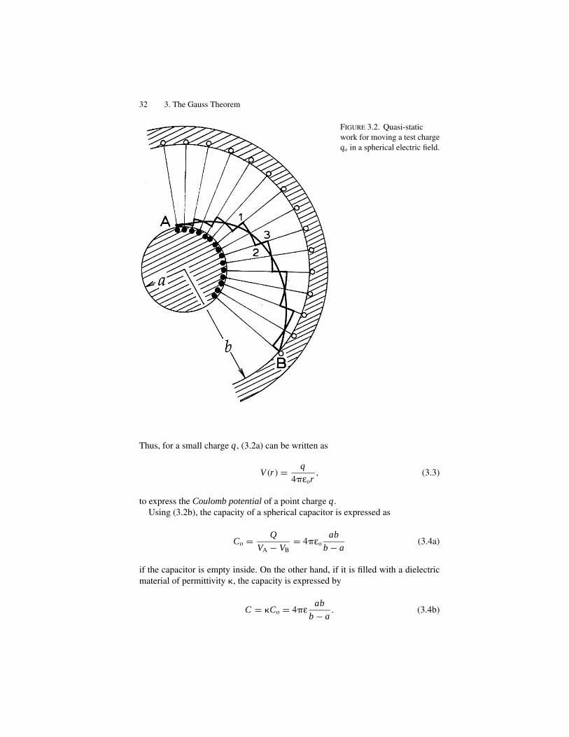
32 3. The Gauss Theorem
FIGURE 3.2. Quasi-static
work for moving a test charge
qo in a spherical electric field.
Thus, for a small charge q , (3.2a) can be written as
V (r ) = q
4�εor, (3.3)
to express the Coulomb potential of a point charge q.Using (3.2b), the capacity of a spherical capacitor is expressed as
Co = Q
VA − VB
= 4�εo
ab
b − a(3.4a)
if the capacitor is empty inside. On the other hand, if it is filled with a dielectricmaterial of permittivity �, the capacity is expressed by
C = �Co = 4�εab
b − a. (3.4b)
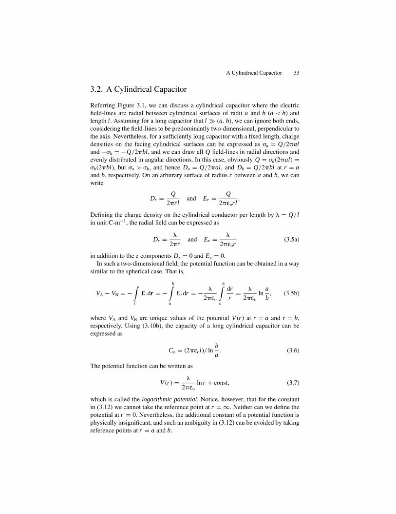
A Cylindrical Capacitor 33
3.2. A Cylindrical Capacitor
Referring Figure 3.1, we can discuss a cylindrical capacitor where the electricfield-lines are radial between cylindrical surfaces of radii a and b (a < b) andlength l. Assuming for a long capacitor that l � (a, b), we can ignore both ends,considering the field-lines to be predominantly two-dimensional, perpendicular tothe axis. Nevertheless, for a sufficiently long capacitor with a fixed length, chargedensities on the facing cylindrical surfaces can be expressed as �a = Q/2�aland −�b = −Q/2�bl, and we can draw all Q field-lines in radial directions andevenly distributed in angular directions. In this case, obviously Q = �a(2�al) =�b(2�bl), but �a > �b, and hence Da = Q/2�al, and Db = Q/2�bl at r = aand b, respectively. On an arbitrary surface of radius r between a and b, we canwrite
Dr = Q
2�rland Er = Q
2�εorl.
Defining the charge density on the cylindrical conductor per length by � = Q/ lin unit C-m−1, the radial field can be expressed as
Dr = �
2�rand Er = �
2�εor(3.5a)
in addition to the z components Dz = 0 and Ez = 0.In such a two-dimensional field, the potential function can be obtained in a way
similar to the spherical case. That is,
VA − VB = −∫�
E.dr = −b∫
a
Er dr = − �
2�εo
b∫a
dr
r= �
2�εo
lna
b, (3.5b)
where VA and VB are unique values of the potential V (r ) at r = a and r = b,respectively. Using (3.10b), the capacity of a long cylindrical capacitor can beexpressed as
Co = (2�εol)/ lnb
a. (3.6)
The potential function can be written as
V (r ) = �
2�εo
ln r + const, (3.7)
which is called the logarithmic potential. Notice, however, that for the constantin (3.12) we cannot take the reference point at r = ∞. Neither can we define thepotential at r = 0. Nevertheless, the additional constant of a potential function isphysically insignificant, and such an ambiguity in (3.12) can be avoided by takingreference points at r = a and b.
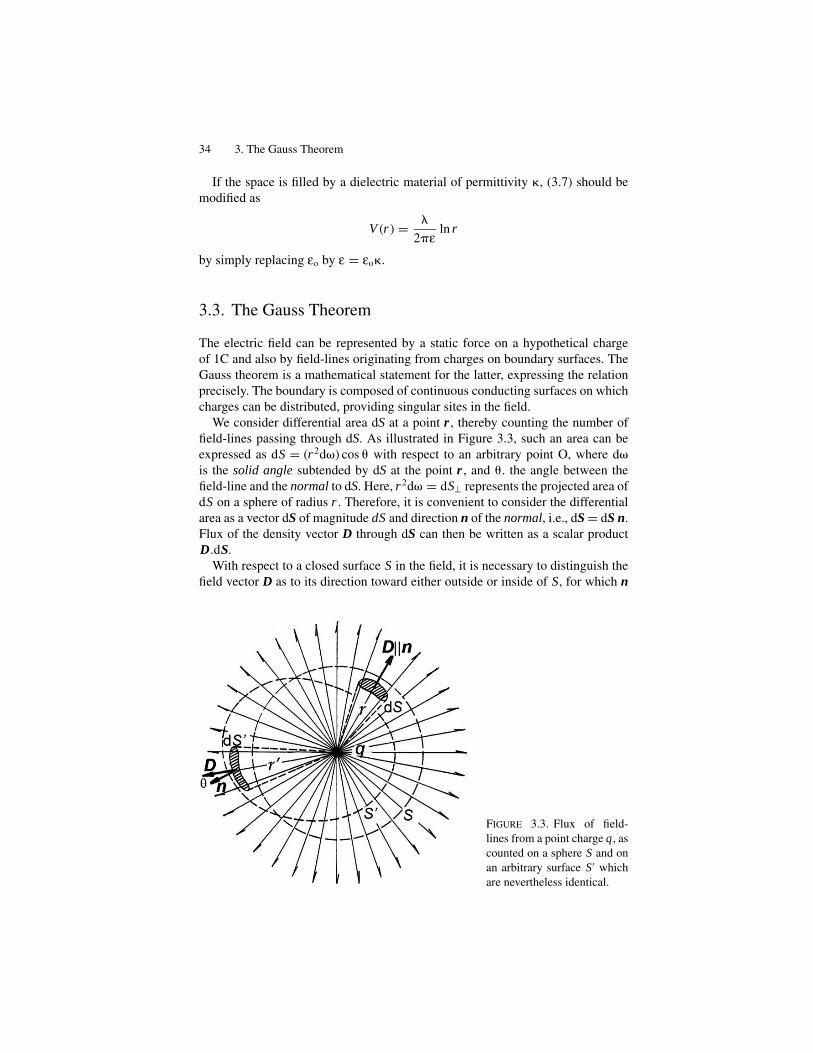
34 3. The Gauss Theorem
If the space is filled by a dielectric material of permittivity �, (3.7) should bemodified as
V (r ) = �
2�εln r
by simply replacing εo by ε = εo�.
3.3. The Gauss Theorem
The electric field can be represented by a static force on a hypothetical chargeof 1C and also by field-lines originating from charges on boundary surfaces. TheGauss theorem is a mathematical statement for the latter, expressing the relationprecisely. The boundary is composed of continuous conducting surfaces on whichcharges can be distributed, providing singular sites in the field.
We consider differential area dS at a point r , thereby counting the number offield-lines passing through dS. As illustrated in Figure 3.3, such an area can beexpressed as dS = (r2d�) cos � with respect to an arbitrary point O, where d�is the solid angle subtended by dS at the point r , and �. the angle between thefield-line and the normal to dS. Here, r2d� = dS⊥ represents the projected area ofdS on a sphere of radius r . Therefore, it is convenient to consider the differentialarea as a vector dS of magnitude dS and direction n of the normal, i.e., dS = dS n.Flux of the density vector D through dS can then be written as a scalar productD.dS.
With respect to a closed surface S in the field, it is necessary to distinguish thefield vector D as to its direction toward either outside or inside of S, for which n
FIGURE 3.3. Flux of field-
lines from a point charge q, as
counted on a sphere S and on
an arbitrary surface S′ which
are nevertheless identical.

The Gauss Theorem 35
is usually defined as the outward normal. With this definition of the vector areawe can see that the total flux of field-lines � etermined by a closed surface S, i.e.,� = ∮
S D.dS, is independent of the choice of S.Considering a point charge q at the origin O as shown in Figure 3.3, the electric
field is radial as expressed by the flux density Dr = q/4�r2, therefore
� =∮S
D.dS =∮S⊥
Dr dS⊥ = q
4�
∮sphere
r2d�
r2= q
4�
∮sphere
d� = q,
which is consistent with the rule for the theoretical number of field-lines to bedrawn from q .
If q is located inside or outside S is significant in this argument, and we noticethat such a surface can be arbitrary in shape for counting field-lines. Therefore,the above relation � = q holds for any arbitrary S, provided that q is inside S, andthis result can be extended to a system of many charges qi (i = 1, 2, . . .) as
� =∮S
D.dS =∑
i
qi = Qinside, (3.8)
where Qinside is the total charge enclosed in S.We can show that a charge qe located outside S has no contribution to the flux �
etermined by S. For a charge qe as shown in Figure 3.4(a), we evaluate fluxes d�1
and d�2 determined by differential areas dS1 = n1(r21 d�1) and dS2 = n2(r2
2 d�2
at points 1 and 2 in the radial line drawn from qe.In this figure, note that the angle �1 between D1 and n1 is an obtuse angle,
whereas �2 between D2 and n2 is an acute one; hence we obtain
d�1 = qe
4�r21
r21 d�1 = qe
4�d�1 and d�2 = − qe
4�d�2,
FIGURE 3.4. Flux of field-lines counted on a closed surface in general shape. (a) A charge
qe outside S. (b) A charge qi inside S.

36 3. The Gauss Theorem
so that
� =∮S
(d�1 + d�2) = qe
4�
∮S
(d�1 − d�2) = 0.
We can thus exclude all charges qe outside S from the calculation of �.To count field-lines the surface S should be continuous and arbitrary in shape.
Nevertheless, some indented surface can be permitted in part on S, as shown inFigure 3.4(b). In this case a radial field-line from inside qi is crosses such anindented S three times (or an odd number of times in general), giving such a totalcontribution that d�1 + d�2 + d�3 = d�1, because d�2 = −d�3.
For an arbitrarily chosen surface S in general, some charges can be inside of Sbut some are outside. However, clearly only those enclosed in S can contribute tothe integral
∮S D.dS. Therefore, (3.8) can represent a general case, where Qinside
is the total charge enclosed inside S, and the relation is called the Gauss theorem.Such a surface S, as chosen for mathematical purposes, is referred to as a Gaussiansurface.
In the above we considered point charges qi and qe for simplicity; howevercharges can also be distributed continuously on surfaces and in a volume as well.Such distributed charges are represented by a differential charge element that can beconsidered as a point charge. For a continuous distribution of charges we can write
Qinside =∫v
� (r ) d3r or
∫S
� (r ) d2r , (3.9)
where � (r ) and �(r ) are volume and surface densities of charges at r , respectively,and d3r and d2r are commonly used notations for volume and surface elementsdv and dS.
Example 1. A Conducting Plate.Figure 3.5 shows a conducting plate of a large area on which a flat cylindrical
surface with a short height is set up as a Gaussian surface, where the top and bottomsurfaces of area A are parallel to the plate.
FIGURE 3.5. A Gaussian surface in the shape of a pillbox on a conducting boundary.

The Gauss Theorem 37
FIGURE 3.6. A Gaussian surface in cylindri-
cal shape for counting field-lines from a long
charged conducting rod.
In fact, this problem is hypothetical, unless we consider another conductor withthe given plate, which is necessary in principle for forming a capacitor. For sucha single charged plate we should consider another one like a spherical conductorwith infinite radius. In such a single plate, charges should reside on both surfacesof the plate, whereas if there is another plate nearby as in a parallel-plate capacitor,all charges appear on the facing surface only. Thus, if the surface charge densityis Q/A = � on parallel plates, it should be reduced to Q/2A = 1
2� on the single
isolated plate.Ignoring the effect near the edges, the field-lines are all parallel to one another
and perpendicular to the plate of infinite area. Applied to the surface of a pillboxshape, the Gauss theorem can be expressed as∮
box
D.dS = (Dn A)top + (Dn A)bottom + (Dn A′)side = 2 × 1
2� A.
Since A = A′, we obtain Dn = 12�, signifying that the field is separated into the
top and bottom of the plate due to separated charge densities 12�.
Example 2. A Long a Conducting Rod.Figure 3.6 shows a long conducting rod, where a concentric cylindrical Gaussian
surface S of radius r and height l is indicated. When we charge it with a battery,however, we have to assume that the rod is a part of a cylindrical uniaxial capacitorthat is composed with another cylinder of radius r = ∞. Further assuming thelength is sufficiently long, the charge Q on the rod can be distributed evenlyon the surface, which is conveniently expressed by the density per unit length,

38 3. The Gauss Theorem
i.e., � = Q/ l. Such a concentric Gaussian surface is an obvious choice for asimple analysis of this case, where the flux-density vector D can be radial andperpendicular to the rod, so that the flux D.dS vanishes on the top and bottomsurfaces. Referring the rod axis to the z-axis, we use cylindrical coordinates (r ,�, z) for a point in the field. The flux � of field-lines determined by S can beexpressed by ∫
S
D.dS =∫ 2�
0
Drrld� = Drrl × 2� = �l,
from which we obtain the expression Dr = �/2�r , that is identical to (3.5a).
Example 3. A Uniformly Charged Sphere.J. J. Thomson (1903) considered a uniformly charged sphere to be a model of
an atom, one in which an electron can vibrate in harmonic motion to emit light.Assuming it to be electrically neutral, such an atom consists of an electron and apositive charge +e. He considered that positive charge uniformly distributed insidea spherical volume of radius R.
Using the Gauss theorem, we can calculate the flux density D at a distance rgreater than R. By symmetry, the vector D should be radial with respect to thecenter and given only by its radial component Dr . Therefore, the Gauss theoremapplied to a spherical surface of radius r > R can be expressed as∮
S
D.dS =∮S
Drr2d� = Drr2
∮S
d� = Dr(4�r2
) = +e,
and hence, at a point r > R, we have
Dr = e
4�r2and Er = e
4�εor2,
implying that such a charged sphere looks as if a point charge located at r = 0when observed at a distant point r > R.
On the other hand, at a point r < R inside the sphere, the electric field can becalculated as arising from the amount of charge enclosed by a sphere S of radiusr , whose flux density is determined by e(r /R)3. Therefore, for such a sphere wecan write
e( r
R
)3
= Dr 4�r2,
and hence
Er = e
4�εo R3r for r < R.
Placing the electron at an inside point r , the force Fr = −eEr = − e2
4�εo R3r is
a restoring force for the electron to be bonded at r = 0, being proportional to r .Considering the kinetic energy, the electron can vibrate in the vicinity of the center,hence emitting its energy as a radiating dipole.
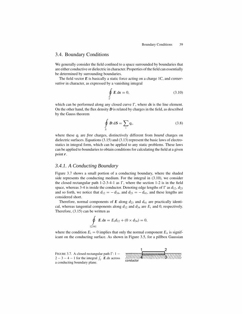
Boundary Conditions 39
3.4. Boundary Conditions
We generally consider the field confined to a space surrounded by boundaries thatare either conductive or dielectric in character. Properties of the field can essentiallybe determined by surrounding boundaries.
The field vector E is basically a static force acting on a charge 1C, and conser-vative in character, as expressed by a vanishing integral∮
�
E.ds = 0, (3.10)
which can be performed along any closed curve �, where ds is the line element.On the other hand, the flux density D is related by charges in the field, as describedby the Gauss theorem ∮
S
D.dS =∑
i
qi, (3.8)
where these qi are free charges, distinctively different from bound charges ondielectric surfaces. Equations (3.15) and (3.13) represent the basic laws of electro-statics in integral form, which can be applied to any static problems. These lawscan be applied to boundaries to obtain conditions for calculating the field at a givenpoint r .
3.4.1. A Conducting Boundary
Figure 3.7 shows a small portion of a conducting boundary, where the shadedside represents the conducting medium. For the integral in (3.10), we considerthe closed rectangular path 1-2-3-4-1 as �, where the section 1-2 is in the fieldspace, whereas 3-4 is inside the conductor. Denoting edge lengths of � as d12, d23
and so forth, we notice that d12 = − d34, and d23 = − d41, and these lengths areconsidered short.
Therefore, normal components of E along d23 and d41 are practically identi-cal, whereas tangential components along d12 and d34 are Et and 0, respectively.Therefore, (3.15) can be written as∮
12341
E.ds = Etd12 + (0 × d34) = 0,
where the condition Et = 0 implies that only the normal component En is signif-icant on the conducting surface. As shown in Figure 3.5, for a pillbox Gaussian
FIGURE 3.7. A closed rectangular path �: 1 −2 − 3 − 4 − 1 for the integral
∫�
E.ds across
a conducting boundary plane.
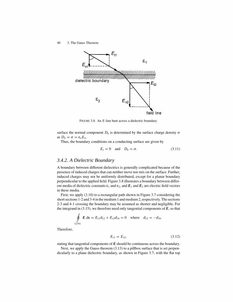
40 3. The Gauss Theorem
FIGURE 3.8. An E-line bent across a dielectric boundary.
surface the normal component Dn is determined by the surface charge density �as Dn = � = εo En .
Thus, the boundary conditions on a conducting surface are given by
Et = 0 and Dn = �. (3.11)
3.4.2. A Dielectric Boundary
A boundary between different dielectrics is generally complicated because of thepresence of induced charges that can neither move nor mix on the surface. Further,induced charges may not be uniformly distributed, except for a planar boundaryperpendicular to the applied field. Figure 3.8 illustrates a boundary between differ-ent media of dielectric constants ε1 and ε2, and E1 and E2 are electric field vectorsin these media.
First, we apply (3.10) to a rectangular path shown in Figure 3.7 considering theshort sections 1-2 and 3-4 in the medium 1 and medium 2, respectively. The sections2-3 and 4-1 crossing the boundary may be assumed as shorter and negligible. Forthe integrand in (3.15), we therefore need only tangential components of E, so that∮
12341
E.ds = Et1d12 + Et2d34 = 0 where d12 = −d34.
Therefore,
Et1 = Et2, (3.12)
stating that tangential components of E should be continuous across the boundary.Next, we apply the Gauss theorem (3.13) to a pillbox surface that is set perpen-
dicularly to a plane dielectric boundary, as shown in Figure 3.7, with the flat top

Boundary Conditions 41
FIGURE 3.9. A charged capacitor filled by
parallel layers of two dielectric materials.
and bottom in dielectric media 1 and 2, respectively. It can then be written as∮box
D.dS = Dn1S1 − Dn2S2 = 0, where S1 = S2.
Hence,
ε1 En1 = ε2 En2, (3.13)
implying that normal components of D are continuous, although the correspondingE is discontinuous across the boundary, because of ε1 = ε2. As remarked, this resultis also due to the fact that no free charges can, normally, exist on the dielectricboundary.
Denoting angles between E and n in two media as �1 and �2, as indicatedin Figure 3.8, we have tan �1 = Et1/En1 and tan �2 = Et2/En2. Using (3.17) and(3.18), we obtain
tan �1
tan �2
= ε1
ε2
, (3.14)
indicating that field-lines bend directions at the boundary, except for �1 = �2 = 0.If E|| n particularly, En is discontinuous, and Et = 0, thereby characterizing the
boundary as an equipotential surface.The conditions (3.17) and (3.18) can generally be applied to static boundaries
between different nonconducting dielectric media, signifying the continuity of Et
and Dn . In contrast, on a conducting surface characterized by E = 0, and so D = 0,the relation Dn = � signifies the discontinuity on a conducting surface. Also, asthe tangential component is zero outside the conductor as well as inside, Et appearsto be continuous.
Example. A Planar Dielectric Boundary in a Capacitor.Consider two dielectric layers of thickness a and b with different dielectric
constants ε1 and ε2 filling the gap d of a parallel-plate capacitor that is charged bya battery, as shown in Figure 3.9.
In this case, these two layers behave like a single medium of an effective di-electric constant ε′ and thickness a + b = d, exhibiting induced charges ∓QP onsurfaces facing the charged capacitor plates at ±Q. On the boundary surface be-tween different dielectric media there appears no macroscopic charge, so that the

42 3. The Gauss Theorem
flux from charges ±Q penetrates continuously into the media, i.e., Dn1 = Dn2,in which another flux of lines from the polarized charges ∓QP exists in rela-tion with Pn1 = Pn2. Here, we have Dn1 − Pn1 = 0 and Dn2 − Pn2 = 0, and soε1 En1 = ε2 En2 = 0, accordingly En1 = En2 = 0 on the boundary. On the otherhand, there is no tangential field in the media, so that the boundary surface shouldbe equipotential, ignoring the gap between the media 1 and 2. Thus, signifyingsurfaces by potentials, V+, V1, and V−, the capacitor can be regarded as equivalentto two capacitors filled with dielectric media ε1 and ε2 that are connected in series.Namely, we can write
C1 = ε1 A
a, C2 = ε2 A
b, C = ε ′
A
dand
1
C= 1
C1
+ 1
C2
,
and
ε′ = 1
a
ε1
+ b
ε2
.
Further, writing that
V+ − V− = Q
C= E(a + b) and Q − QP = εo E,
we obtain
QP = Q
⎛⎜⎝
1 + εo
a
ε1
+ b
ε2
a + b
⎞⎟⎠
.

5The Legendre Expansion of Potentials
5.1. The Laplace Equation in Spherical Coordinates
In electrostatics a basic problem is to find the potential function for a given chargedistribution that can be solved with the Laplace-Poisson equations under specifiedboundary conditions. Although the cause for distributed charges is unspecifiedin the given system, here we are only concerned about the electrostatic problem.For many applications we are interested in the potential at a distant point fromdistributed charges in a small region. The corresponding field is often dominated bydeviations from spherical symmetry, a deviation that can be conveniently viewedwith polar coordinates with respect to the center of distribution. Such a chargedistribution is often described with respect to a unique direction for deformationthat arises from an internal origin.
The Laplace equation ∇2V = 0 is a partial differential equation to which themethod of separating variables is applied, reducing it to a set of ordinary differ-ential equations for the individual curvilinear coordinates. In polar coordinatesr, �, and �, the Laplace equation can be expressed as
1
r2
∂
∂r
(r2 ∂V
∂r
)+ 1
r2 sin �
∂
∂�
(sin �
∂V
∂�
)+ 1
r2 sin2 �
∂2V
∂�2= 0. (5.1)
Assuming V (r, �, �) = R(r )�(�)�(�), where the factors R, �. and �. are functionsof r , �, and �, respectively, equation (5.1) can be written as
1
r2 R
d
dr
(r2 dR
dr
)+ 1
r2� sin �
d
d�
(sin �
d�
d�
)+ 1
r2� sin2 �
d2�
d�2= 0. (i)
First, we let
d2�
d�2= −m2�, (ii)
from which we have
�(�) = �o exp (±im�).
64

The Laplace Equation in Spherical Coordinates 65
In order for the potential to assume a unique value, we must consider that �(�) =�(� + 2�), so that m is determined from exp (±2m�i) = 1. Therefore, m mustbe either 0 or ± an integer, i.e., m = 0, ±1, ±2, . . . .
Next, in (i) we set
1
R
d
dr
(r2 dR
dr
)= k, (iii)
in order to obtain a radial function that can be expressed as R(r ) = Arn, where nis an integer. Then, from (iii) k should be related to n as given by
k = n(n + 1). (iv)
It is noted that (iv) can also be fulfilled by another integer n′ = −(n + 1), as wecan write k = n′(n′ + 1). Therefore, generally, the function R(r ) can be expressedas
R(r ) = Anrn + Bn
rn+1, (v)
where An and Bn are constants for R(r ) to be determined as a linear combination ofthese terms of rn and 1/rn+1, as required by boundary conditions. For the positiver , it is sufficient to consider that n = 0, 1, 2, 3, . . . .
Using (ii) and (iv) in the relation (i), we obtain the equation for �(�) expressedas
n(n + 1) + 1
� sin �
d
d�
(sin �
d�
d�
)− m2
sin2 �= 0,
and hence the function �(�) depends generally on indexes n and m. However,noting that the specific case of m = 0 signifies the potential independent of theangle �, such an axially symmetric function is specified only by the index n.Therefore, the function � for m = 0 is specially written as Pn(�). For the axialfunction Pn(�), called the Legendre function, we have a differential equation
1
sin �
d
d�
(sin �
dPn
d�
)+ n (n + 1) Pn = 0, (5.2a)
which can also be expressed in terms of a variable � = cos �; that is,
d
d�
{(1 − �2) dPn
d�
}+ n (n + 1) Pn = 0 (5.2b)
Noting that the equation (5.2b) is unchanged when n is replaced by −(n + 1), wehave the relation
Pn(cos �) = P−n−1(cos �) (5.3)
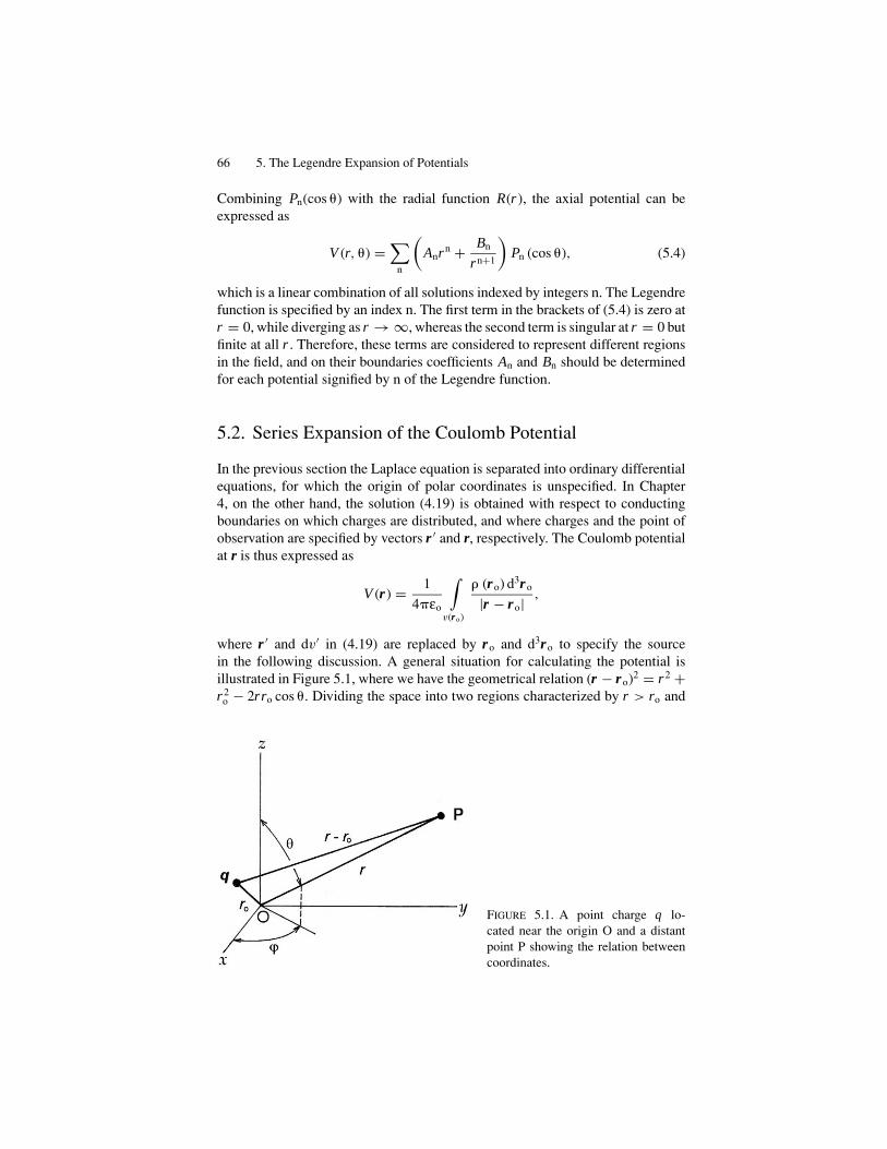
66 5. The Legendre Expansion of Potentials
Combining Pn(cos �) with the radial function R(r ), the axial potential can beexpressed as
V (r, �) =∑
n
(Anrn + Bn
rn+1
)Pn (cos �), (5.4)
which is a linear combination of all solutions indexed by integers n. The Legendrefunction is specified by an index n. The first term in the brackets of (5.4) is zero atr = 0, while diverging as r → ∞, whereas the second term is singular at r = 0 butfinite at all r . Therefore, these terms are considered to represent different regionsin the field, and on their boundaries coefficients An and Bn should be determinedfor each potential signified by n of the Legendre function.
5.2. Series Expansion of the Coulomb Potential
In the previous section the Laplace equation is separated into ordinary differentialequations, for which the origin of polar coordinates is unspecified. In Chapter4, on the other hand, the solution (4.19) is obtained with respect to conductingboundaries on which charges are distributed, and where charges and the point ofobservation are specified by vectors r ′ and r, respectively. The Coulomb potentialat r is thus expressed as
V (r ) = 1
4�εo
∫v(ro)
� (ro) d3ro
|r − ro| ,
where r ′ and dv′ in (4.19) are replaced by ro and d3ro to specify the sourcein the following discussion. A general situation for calculating the potential isillustrated in Figure 5.1, where we have the geometrical relation (r − ro)2 = r2 +r2
o − 2rro cos �. Dividing the space into two regions characterized by r > ro and
FIGURE 5.1. A point charge q lo-cated near the origin O and a distantpoint P showing the relation betweencoordinates.
Series Expansion of the Coulomb Potential 67
r < ro, we have
1
|r − ro| = 1
r√
1 − 2�s + �2, where s = ro
r,
and1
|r − ro| = 1
ro
√1 − 2�s + s2
, where s = r
ro,
respectively, where the factor (1 − 2�s + s2)−1, known as the generating function,can be expanded into power series for a small variable s. That is,
1√1 − 2�s + s2
= 1 + �s + 1
2(3�2 − 1)s2 + 3
2(5�3 − 3�)s3
+1
8(35�4 − 30�2 + 3)s4 + . . . ,
where the coefficients can be identified as Legendre’s functions Pn(�) for n =0, 1, 2, 3, . . . . Leaving the proof to Section 5.3, we write the series expansion as
1√1 − 2�s + s2
=∑
n
Pn (�) sn, (5.5)
where
P0(�) = 1, P1(�) = �, P2(�) = 1(3�2 − 1), P3(�) = (5�3 − 3�), . . . .
Using Pn(�), the Coulomb potential for the region r > ro can be expressed by
V (r ) = 1
4�εo
∑n
Pn (�)
rn+1
∫v(ro)
� (ro) rno d3ro, (5.6a)
whereas, for r < ro ,
V (r ) = 1
4�εo
∑n
rn Pn (�)∫
v(ro)
� (ro)
rn+1o
d3ro. (5.6b)
The potential V (r ) of (5.6a) and (b) are expressed as a superposition of componentpotentials Vn(r ) for n = 0, 1, 2, . . . , that is, V (r ) = �nVn(r ).
In the region for r > ro in particular, for n = 0,
Vo(r ) = 1
4�εo
Q
r, where Q =
∫v(ro)
� (ro) rod3ro
represents a point charge model effectively for the total charge Q. For n = 1,
V1(r ) = 1
4�εo
p cos �
r2, where p =
∫v(ro)
� (ro) rod3ro
expresses the dipole moment associated with distributed charges.
68 5. The Legendre Expansion of Potentials
5.3. Legendre’s Polynomials
We discuss the Legendre function briefly in this mathematical section. Here, forthe function Pn(�) defined as expansion coefficients in (5.5), we show the proofthat Pn(�) satisfies the equation (5.2b), and the recurrence formula.
Differentiating (5.5) with respect to the variable s, we obtain� − s(
1 − 2�s + s2) 3
2
=∑
n
nsn−1 Pn (�).
Using (5.5) in this expression, we can write
(� − s)∑
n
Pn (�) sn =∑
n
(nsn−1 + nsn + 1 − 2nsn) Pn (�)
and, hence,∑n
(2n + 1) �sn Pn (�) =∑
n
(n + 1) sn+1 Pn (�) +∑
n
nsn−1 Pn (�)
We can compare terms of sn on both sides of this relation and obtain a recurrenceformula,
(2n + 1) �Pn (�) = (n + 1) Pn+1 (�) + nPn−1 (�) . (5.7)
For positive values, k = n(n + 1) ≥ 0, the order n can be equal to −1, 0, 1, 2, . . . ,therefore from (5.7) we can write, successively, that
P−1(�) = 0, P0(�) = 1, P1(�) = �P0(�) = �,
2P2(�) = 3�P1(�) − P0(�) = 3�2 − 1,
P3(�) = 5�P2(�) − 2P1(�) = 1
2(15�3 − 9�), . . . .
Thus, the expansion coefficients Pn(�) in the series (5.5), known as the Legendrepolynomials, are related by the recurrence formula (5.7).
Next, we differentiate (5.5) with respect to the variable �, and obtain
s(1 − 2�s + s2
) 32
=∑
n
sn P ′n (�), where P ′
n (�) = dPn (�)
d�.
Hence,
s
(∑n
sn Pn (�)
)= (
1 − 2�s + s2) ∑n
sn P ′n (�).
Equating the coefficient of sn on the left side to those on the right, we obtainanother recurrence formula,
Pn(�) = P ′n+1(�) + P ′
n−1(�) − 2�P ′n(�). (5.8)
Next, we derive the Legendre equation (5.2b) using these recurrence formulas toshow that Pn(�) is the solution. Differentiating (5.7) with respect to �, we obtain
(2n + 1){
Pn (�) + �P ′n (�)
} = (n + 1) P ′n+1 (�) + nP ′
n−1 (�) ,
A Conducting Sphere in a Uniform Field 69
and so
(2n + 1) Pn (�) = (n + 1) P ′n+1 (�) + nP ′
n−1 (�) − (2n + 1) �P ′n (�)
= n{
P ′n+1 (�) + P ′
n−1 (�) − 2�P ′n (�)
} + P ′n+1 (�) − �P ′
n (�)
or
(2n + 1)Pn(�) = (n + 1){
P ′n+1 (�) + P ′
n−1 (�) − 2�P ′n (�)
}−P ′
n−1 (�) + �P ′n (�) .
Using (5.7), we can replace the quantity in the curly brackets by Pn(�), and
(n + 1) Pn (�) = P ′n+1 (�) − �P ′
n (�) or nPn (�) = −P ′n−1 (�) + �P ′
n (�) .
The first expression can be written as nPn−1 (�) = P ′n (�) − �P ′
n−1 (�) by chang-ing n to n − 1. Eliminating P ′
n−1(�) from this and the second expression, we obtain
nPn−1 (�) = �nPn (�) + (1 − �2) P ′
n (�) .
Therefore,
d
d�
{(1 − �2) P ′
n (�)}=n
{P ′
n−1 (�) − �P ′n (�)
}− nPn (�)=−n (n + 1) Pn (�) ,
which is the Legendre equation (5.2b).
5.4. A Conducting Sphere in a Uniform Field
A conducting sphere is polarized in a uniform field, which becomes axially sym-metric in the vicinity of the field, although almost unchanged at distant places.Induced charges appear on the spherical surface, producing an axial field thatmodifies the original uniform field.
For such a problem, polar coordinates r, �, and � can be used with respect tothe direction of the uniform field passing through the center of the sphere. In thiscase, at the distant point the field Eo is constant and expressed by the potentialV = −Eoz, that is,
V (r, �) = −Eor cos � for r → ∞, (i)
which is regarded as the condition for the potential to satisfy in the distant regionfrom the sphere. On the other hand, the potential must also be constant on theconducting spherical surface of radius R, and hence
V (R, �) = Vo(constant) (ii)
is the other boundary condition to be satisfied, and it can also be expressed by
E� = 0 and εo Er = �P at r = R. (iii)
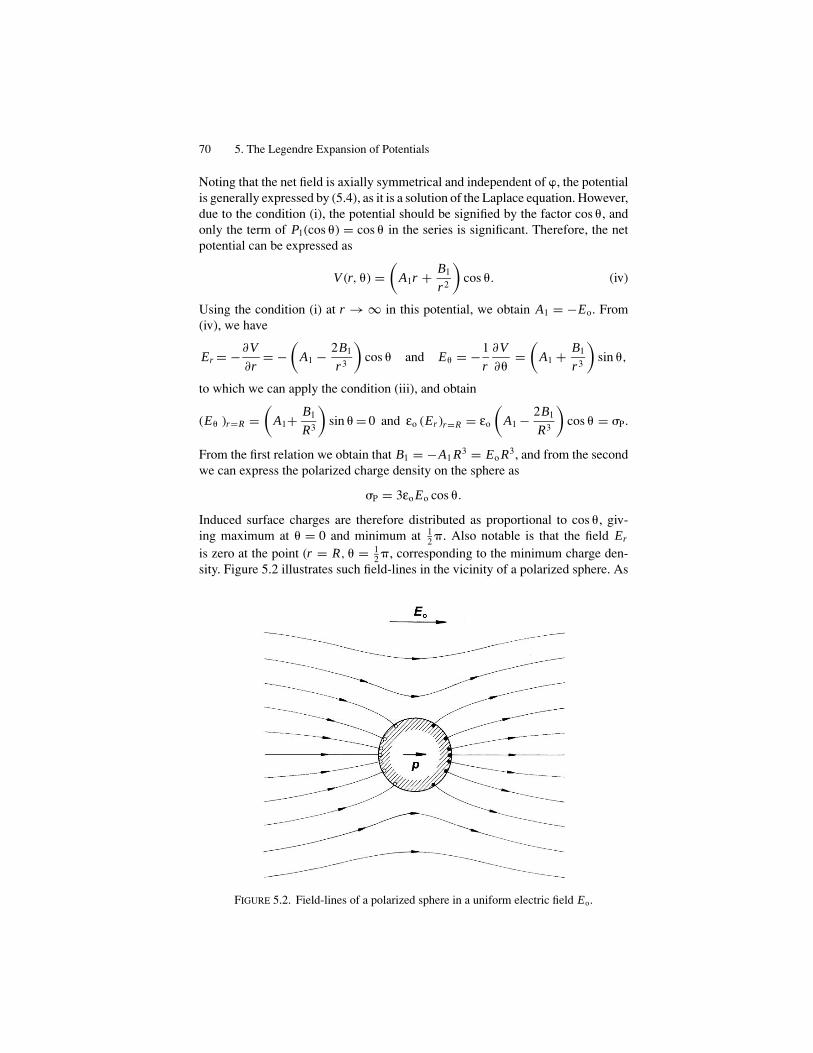
70 5. The Legendre Expansion of Potentials
Noting that the net field is axially symmetrical and independent of �, the potentialis generally expressed by (5.4), as it is a solution of the Laplace equation. However,due to the condition (i), the potential should be signified by the factor cos �, andonly the term of P1(cos �) = cos � in the series is significant. Therefore, the netpotential can be expressed as
V (r, �) =(
A1r + B1
r2
)cos �. (iv)
Using the condition (i) at r → ∞ in this potential, we obtain A1 = −Eo. From(iv), we have
Er = −∂V
∂r= −
(A1 − 2B1
r3
)cos � and E� = −1
r
∂V
∂�=
(A1 + B1
r3
)sin �,
to which we can apply the condition (iii), and obtain
(E� )r=R =(
A1+ B1
R3
)sin � = 0 and εo (Er )r=R = εo
(A1 − 2B1
R3
)cos � = �P.
From the first relation we obtain that B1 = −A1 R3 = Eo R3, and from the secondwe can express the polarized charge density on the sphere as
�P = 3εo Eo cos �.
Induced surface charges are therefore distributed as proportional to cos �, giv-ing maximum at � = 0 and minimum at 1
2 �. Also notable is that the field Er
is zero at the point (r = R, � = 12 �, corresponding to the minimum charge den-
sity. Figure 5.2 illustrates such field-lines in the vicinity of a polarized sphere. As
FIGURE 5.2. Field-lines of a polarized sphere in a uniform electric field Eo.
A Dielectric Sphere in a Uniform Field 71
indicated by (iv), the potential is given by a superposition of a uniform potential−Eor cos � plus a dipole potential V1 = p/4�εor2, where the dipole moment isdefined as p = (4�εo)Eo R3.
5.5. A Dielectric Sphere in a Uniform Field
In this section, we discuss a dielectric sphere that is polarized by a uniform electricfield. We assume that the material is of a uniform density and characterized bya dielectric constant ε. As is true for a conducting case, such a sphere is in axialsymmetry, however unlike in a conductor, there is an electric field inside the sphere.We describe the field by coordinates r and � with respect to the center of thesphere, referring to the direction of applied field expressed at distant points by thepotential
V = −Eoz = −Eor cos �.
The potential V (r, �) can be expressed outside and inside the sphere as
Vout(r, �) = −Eor cos � +∑
n
Bn
rn+1Pn (cos �) for r > R
and
Vin(r, �) =∑
n
Anrn Pn (cos �) for r < R,
respectively. The boundary conditions on the spherical surface are
Vout(R, �) = Vin(R, �)
and
−εo
(∂Vout
∂r
)r=R
= −ε(
∂Vin
∂r
)r=R
We can find that the coefficients An and Bn for n > 1 cannot satisfy these boundaryconditions simultaneously, and, consequently, only A1 and B1 need be determined,as in the case of a conducting sphere. Thus, for n = 1 the conditions are written as
−Eo R + B1
R2= A1 R and − εo
(Eo
2B1
R3
)= ε A1.
Solving these for A1 and B1, we obtain
A1 = 3εo Eo
ε + 2εoand B1 = ε − εo
ε + 2εoEo R3.
Hence
Vout(r, �) = −Eor cos � + ε − εo
ε + 2εo
Eo R3 cos �
r2

72 5. The Legendre Expansion of Potentials
and
Vin (r, �) = − 3εo
ε + 2εoEor cos �.
The potential Vout(r, �) is composed of uniform and dipolar terms, whereas thepotential Vin(r, �) gives a uniform field.
Replacing r cos � in Vin(r, �) by z,
Ez = −∂Vin (z)
∂z= 3εo
ε + 2εoEo,
which is constant, but not equal to Eo unless ε = εo. Further, the induced surfacecharge density on the sphere can be calculated as
�P = −εo
(∂Vout (r, �)
∂r
)r=R
+ ε(
∂Vin (r, �)
∂r
)r=R
= 2 (ε − εo)
ε + 2εoEo cos �,
which is a maximum at � = 0 and minimum at 12 �. From Vout(r, �), the dipole
moment induced in a dielectric sphere can be written as
p = 4�εo� − 1
� + 2Eo R3, where � = ε
εo.
Also, the electric field outside the sphere can be calculated as
Er − ∂Vout (r, �)
∂r=
{1 + 2 (� − 1)
� + 2
R3
r3
}Eo cos �
E� = −1
r
∂Vout (r, �)
∂�=
{1 − 2 (� − 1)
� + 2
R3
r3
}Eo sin �.
We note that at � = 12 �, while Er = 0, the field is dominated by E� , which is less
than 1; this is because � > 1 signifies a low flux density in this vicinity, as sketchedin Figure 5.3(a).
Exercise. A Spherical Cavity in a Dielectric Medium.Consider a spherical cavity of radius R in a medium of dielectric constant
ε = �εo, as shown in Figure 5.3(b). In this case, the cavity is polarized by anapplied field in the medium. Obtain the expressions for the electric field vectors inthe medium as well as in the cavity, and explain that the field pattern is as illustratedin the figure.
5.6. A Point Charge Near a Grounded Conducting Sphere
In Section 4.7 we discussed an electric image −q of a point charge q on a conduct-ing plane of infinite area. The potential of the plane is regarded as zero because itis extended to infinity. In this section we discuss a conducting sphere of radius Rin the field of a point charge q1, to see if an image charge – q2 can represent the

A Point Charge Near a Grounded Conducting Sphere 73
FIGURE 5.3. A dielectric sphere in auniform electric field Eo. (a) εinside >
εoutside, (b) εinside < εoutside.
sphere. However, for such an image to exist it is realized that the sphere should begrounded to maintain the potential at zero. Otherwise, the sphere is polarized, andnot represented by a dipole moment. On the grounded sphere, the induced chargescan of one kind reside, keeping the other kind away at infinity, so that the spherecan effectively be represented by a charge −q2. Figure 5.4(b) shows a sketch offield-lines near the sphere and q1, where some of the lines from q1 are ended atthe conducting surface, whereas other lines are extended to infinity. Hence, themagnitude of the image charge cannot be of the same as q1.
We calculate the potential V (r1, r2) at a point P, where r1 and r2 are the distancesfrom a given q1 and a hypothetical q2, as shown in Figure 5.4(b). Taking P at exactlyon a surface point of the sphere, we have
V (P) = V (r1, r2) = 1
4�εo
(q1
r1− q2
r2
)= 0.
Indicating the positions of q1 and q2 as z = a and b, respectively, referring to therectangular axes x, y, and z shown in the figure,
r21 = x2 + y2 + (z − a)2 = r2 − 2az + a2

74 5. The Legendre Expansion of Potentials
FIGURE 5.4. A point charge q1 and agrounded conducting sphere. (a) Theelectric image q2. (b) Field-lines dueto q1 and its image q2.
and
r22 = x2 + y2 + (z − b)2 = r2 − 2bz + b2,
where r = (x2 + y2 + z2)1 is the radial distance from the center of the sphere. Atall points on the sphere r = R, V (P) = 0, and hence
q1√R2 − 2az + a2
= q2√R2 − 2bz + b2
,
from which we obtain(q2
1 − q22
)R2 − 2z
(q2
1 b − q22 a
) + q21 b2 − q2
2 a2 = 0.
In order for this equation to be held at all points on the surface, the second termon the right should vanish regardless of z, and therefore
q21 b − q2
2 a = 0 and R2 = q22 a2 − q2
1 b2
q21 − q2
2
.
Accordingly, for the image charge −q2 we have
b = R2
aand q2 = q1
√b
a,
indicating q2 < q1.

A Simple Quadrupole 75
The induced charge density can be calculated with the potentials of point chargesq1 and q2, that is, �(�) = −εo(∂V/∂r )r=R . Writing = R/a for convenience, theresult can be expressed as
�(�) = − q1 (1 − )
4�R2(1 − 2 cos � − 2
) 32
,
giving distributed densities as a function of �, as sketched in Figure 5.4(b). Thetotal induced charge can be obtained by
+1∫−1
� (�) 2�R2d (cos �) = −q1 = q2,
as expected. Further, the force between q1 and −q2 is attractive, and expressed by
F = − 1
4�εo
q1q2
(a − b)2 = − q21
4�εo R2
3
(1 − 2
)2 .
5.7. A Simple Quadrupole
As a simple example of a quadrupole, we consider a spherical charge Q that isdistorted by four external point charges, two positive and two negative, locatedclose to Q on the x- and y-axis, respectively, as illustrated in Figure 5.5.
This is a model for an ionic charge distorted at a lattice site of a rectangularcrystal, where the deformed charge is characterized by four small point charges+q, −q, +q and – q to express a distortion from the spherical Q, as schematicallyshown in the figure. Assuming that such charge displacements occur in the xy-plane,the potential of such a quadrupole can be expressed with polar coordinates r, �, and� with respect to the z-axis. For convenience, we denote these charge deviations
FIGURE 5.5. A simple quadrupolemoment.

76 5. The Legendre Expansion of Potentials
as qi(i = 1, 2, 3, 4) that are located at ai: (a,1
2�, �i), where �i = 0,
1
2�, �,
3
2�,
respectively. For a point P(r, �, �) of observation, we use angles i defined bycos i = (r. ai)/rai. In this case, we have
cos 1 = − cos 3 = sin � cos � and cos 2 = − cos 4 = sin � sin �
and the potential at P can be written for r � ai as
V (r, �, �)= 1
4�εo
∑n
an
rn+1{Pn (cos 1)−Pn (cos 2)+Pn (cos 3)−Pn (cos 4)} .
By the relation (5.3),
Pn(cos 3)= Pn(− cos 1)= (−1)n Pn(cos 1) and Pn(cos 4)= (−1)n Pn(cos 2)
Therefore, the n = 0 and 1 terms can be disregarded, and the n = 2 terms aresignificant for the quadrupole potential, that is
V2(r, �, �) = qa2
2�εor3{P2 (sin � cos �) − P2 (sin � sin �)}
= qa2
2�εor3
(3
2sin2 � cos 2�
)= 1
4�εo
3qa2
r3sin2 � cos 2�.
Exercises.1. In the above model the quadrupole may be considered as consisting of two
dipoles of (q, −q) and l = √2a. Show such a model of two dipoles from which
the same expression for V2 can be obtained.2. Assuming that four charges q in the model are all of the same sign, obtain the
expression of the potential V for r � a.
5.8. Associated Legendre Polynomials
The Coulomb potential (4.19) has been expanded into the Legendre series. Wediscussed the cases of n = 0 and n = 1 for a point charge and dipole; further,a simple quadrupole potential was described as given by n = 2 in the previoussection. Cases for n > 2 can be discussed, also, however, no significant applicationsto practical problems can be found. In contrast, functions P1 and P2 are of specificimportance in applications to molecular dipoles, nuclear quadrupoles, antennadesign, and many other problems.
In symmetry lower than uniaxial, a charge system is signified not only by � butalso by the azimuthal angle �, and the potential has a factor �(�) = �o exp(im�),where m can take zero and ± integer values. For such a potential, the angularfactor is fully expressed as Pn(cos �)exp(im�) = Pm
n (�, �), which is called theassociated Legendre function. The function Pm
n (�, �) is determined as solutions
Associated Legendre Polynomials 77
of the differential equation
sin �d
d�
(sin �
dPmn
d�
)+ {
n (n + 1) sin2 � − m2} Pmn = 0, (5.9a)
or using � = cos � instead of �,
d
d�
{(1 − �2) dPm
n
d�
}+
{n (n + 1) − m2
1 − �2
}Pm
n = 0, (5.9b)
which is called the associated Legendre equation. The function Pmn (�, �) has
singularities at � = ±1 if n and m are integers and n ≥ |m|, constituting physicallymeaningful solutions in the ranges of 0 ≤ � ≤ � and 0 ≤ � ≤ 2�. Mathematically,there is another solution known as the second kind solution, but we disregardit, since only the Pm
n (�, �) are meaningful. Leaving the mathematical detail toreference books, here we discuss only Pm
n (�, �), called the first kind, for potentialproblems.
The associated function Pmn (�, �) can be derived from the Legendre polynomial
Pn(�) by differentiations, i.e.,
P |m|n (�) = (−1)|m| (1 − �2)|m|/2 d|m| Pn (�)
d�|m| . (5.10)
In the Appendix, a proof is given for (5.10) to satisfy the associated Legendreequation (5.9b), showing the orthogonality relation
+1∫−1
P |m|n (�) P |m|
n′ (�) d� = 2
2n + 1
(n + |m|)!(n − |m|)!n,n′ , (5.11)
where n,n′ = 1 if n = n′, otherwise n,n′ = 0 for n = n′, and clearly n ≥ |m| for theassociated function to be real. The normalized Legendre functions, called sphericalharmonics, are then expressed as
Yn,m(�, �) =√
(2n + 1) (n − m)!
4� (n + m)!Pm
n (cos �) exp(im�), (5.12)
for which the orthogonality relation can be written as
2�∫0
�∫0
Yn,m (�, �) Yn′,m′ (�, �)∗ sin �d�d� = 0. (5.13)
It is realized that these spherical harmonics for m = n, n − 1, n − 2, . . . , −nconstitute an orthonormal set of functions, so that Legendre’s function Pn(cos �)can be expressed as a linear combination of these spherical harmonics for m. Inthis connection, we can derive a formula, known as the addition theorem, which isimportant for a multipole expansion of the potential, to be discussed in Section 5.9.Considering an angle � between two given directions (�, �) and (�′, �′), we look

78 5. The Legendre Expansion of Potentials
for the formula forPn(cos � ) to be expressed by these angles. Corresponding tothe cosine law, i.e.,
cos � = cos � cos �′ + sin � sin �′ cos(� − �′),
we can prove the relation
Pn(cos � ) = 4�
2n + 1
−n∑m=+n
Yn,m (�, �) Yn,m∗(�′, �′). (5.14)
Proof: First, we write that
Pn(cos � ) =−n∑
m=n
Anm Pmn (cos �) exp (im�), (i)
where
Anm = 2n + 1
4�
(n − |m|)!(n + |m|)!
2�∫0
d�
−1∫+1
d (cos �)Pn (cos � ) P |m|n (cos �) exp (i |m| �).
Considering a direction (�, �), we can also write that
P |m|n (cos �) exp (i |m| �) =
−n∑m′=+n
Bnm′ P|m′|n (cos � ) exp
(i∣∣m′∣∣ �
), (ii)
where
Bnm′ = 2n + 1
4�
(n − ∣∣m′∣∣)!
(n + |m′|)!
2�∫0
d�
−1∫+1
d (cos � ) P |m|n (cos �) exp (i |m| �) P
|m ′|n
× (cos �) exp(i(m′) �
). (iii)
If we set � = 0 in (ii), we have � = �′ and � = �′, and then from (ii)
Pmn (cos �′) exp(im�′) =
−n∑m′=+n
Bnm′ Pm′n (1) exp
(im′�
) = Bn0 P0n (1) = Bn0.
Writing (iii) for m′ = 0, we also obtain
Bn0 = 2n + 1
4�
2�∫0
d�
−1∫+1
d (cos � ) Pn (cos � ){
Pmn (cos �) exp (im�)
},
and the relation between them indicates that Pn (cos � ) is the coefficient of thespherical harmonic Yn,m(�′, �′) when Yn,m(�, �) is expressed as a linear expansionwith respect to �′ and �′. Thus, taking the normalization factor into account, wearrive at the addition theorem for spherical harmonics (5.14).

Multipole Potentials 79
5.9. Multipole Potentials
The potential function satisfying the Laplace equation can be expressed generallyin two regions r > ro and r < ro: Using (5.14), for the first case, we have
V (r, �, �) = 1
4�εo
∑n
1
rn+1
∑m
Mn,mYn,m (�, �), (5.15a)
where the multipole potentials are expressed as
Mn,m = 4�
2n + 1
∫v(ro)
� (ro) rno Yn,m
∗ (�, �)d3ro. (5.15b)
For the second case,
V (r, �, �) = 1
4�εo
∑n
rn Nn,mYn,m (�, �), (5.16a)
where
Nn,m = 4�
2n + 1
∫v(ro)
� (ro)
rno
Yn,m∗ (�, �)d3ro. (5.16b)
Nevertheless, we are only concerned about the first region r > ro, where a chargecloud can be expressed in terms of multipoles. Equation (5.15a) indicates that thepotential is given by a superposition of potentials characterized by indexes n, andhence written as
V (r, �, �) =∞∑
n=0
Vn (r, �, �), (5.17)
where
Vo = 1
4�εorM0,0,
V1 = 1
4�εor2
(M1,1Y1,1 + M1,0Y1,0 + M1,−1Y1,−1
),
V2 = 1
4�εor3
(M2,2Y2,2 + M2,1Y2,1 + M2,0Y2,0 + M2,−1Y2,−1 + M2,−2Y2,−2
),
and so on. The term Vo is a point-charge potential, where M0,0 = ∫v � (ro)d3ro
represents a charge q . For the potential V1,
Y1,±1 = ±√
3
8�sin � exp (±i�) = ±
√3
8�
x ± iy
rand
Y1,0 =√
3
4�cos � =
√3
4�
z
r,

80 5. The Legendre Expansion of Potentials
which are direction cosines of the vector r, and hence
M1,±1 = 4�
3
√3
8�
∫v(ro)
� (ro) (xo ∓ iyo) d3ro
and
M1,0 = 4�
3
√3
8�
∫v(ro)
� (ro) zod3ro,
where the integrals are components of a dipole moment p = ∫v � (ro)rod3ro.For the potential V2 we have five spherical harmonics for n = 2 and m =
2, 1, 0, −1, −2, which are
Y2,±2 = 1
2
√15
8�
(x ± iy)2
r2,
Y2,±1 = ±√
15
8�
(x ± iy) z
r2, Y2,0 = 1
2
√5
4�
2z2 − x2 − y2
r2,
and
M2,±2 = 2�
5
√15
8�
∫v(ro)
� (ro) (xo ∓ iyo)2 d3ro,
M2,±1 = ±4�
5
√15
8�
∫v(ro)
� (ro) (xo ∓ iyo) zod3ro,
M2,0 = 2�
5
√5
4�
∫v(ro)
� (ro)(2z2
o − x2o − y2
o
)d3ro.
Using these results, the potential V2 can be expressed in a quadratic form,
V2 = 1
8�εor5
(Qxx x2 + Qyy y2 + Qzzz2 + 2Qyz yz + 2Qzx zx + 2Qxy xy
)
where
Qxx =∫
v(ro)
� (ro)(2x2
o − y2o − z2
o
)d3ro, Qxy =
∫v(ro)
� (ro) xo yod3ro, etc.
If these quantities Qij, where i, j = x, y, z, are considered elements of a tensor Q,the potential V2 can be written as
V2 = 1
4�εo
〈r |Q| r〉2r5
, (5.18)
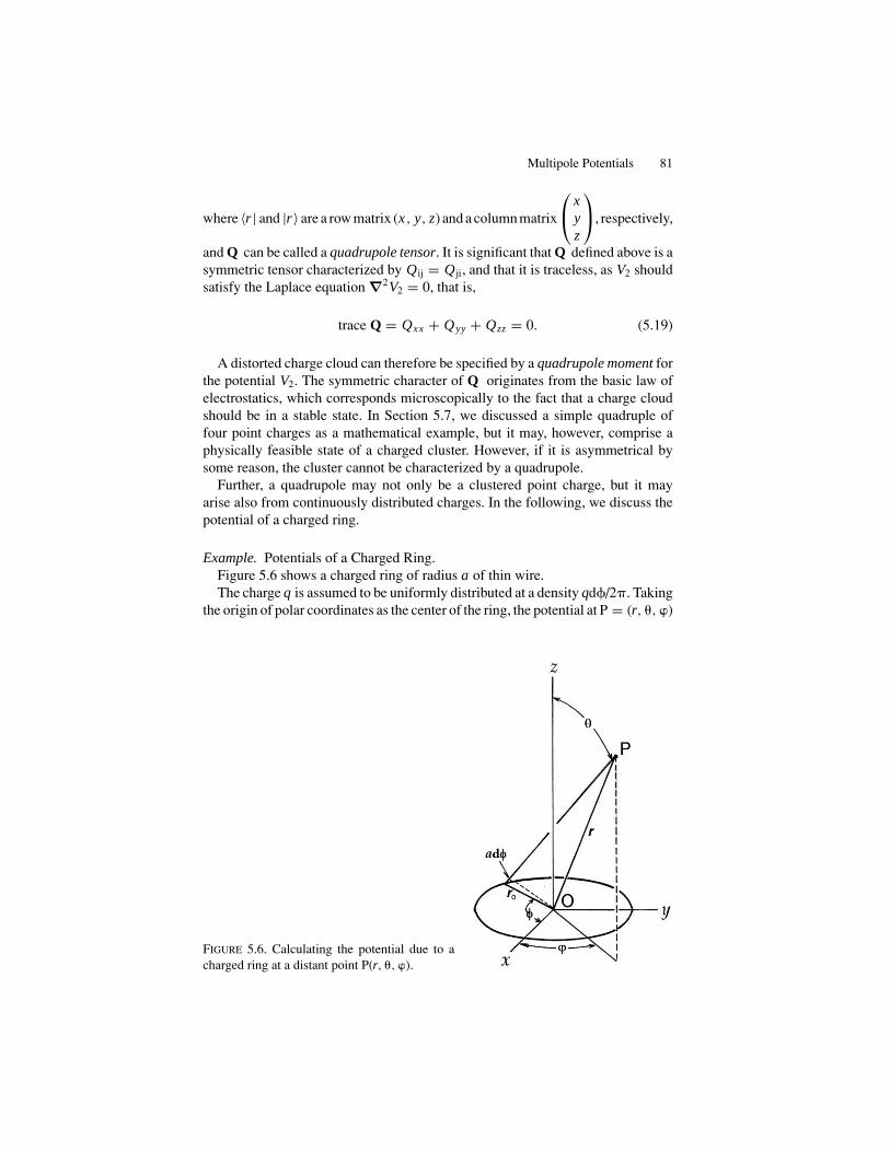
Multipole Potentials 81
where 〈r | and |r〉 are a row matrix (x, y, z) and a column matrix
⎛⎝ x
yz
⎞⎠, respectively,
and Q can be called a quadrupole tensor. It is significant that Q defined above is asymmetric tensor characterized by Qij = Qji, and that it is traceless, as V2 shouldsatisfy the Laplace equation ∇2V2 = 0, that is,
trace Q = Qxx + Qyy + Qzz = 0. (5.19)
A distorted charge cloud can therefore be specified by a quadrupole moment forthe potential V2. The symmetric character of Q originates from the basic law ofelectrostatics, which corresponds microscopically to the fact that a charge cloudshould be in a stable state. In Section 5.7, we discussed a simple quadruple offour point charges as a mathematical example, but it may, however, comprise aphysically feasible state of a charged cluster. However, if it is asymmetrical bysome reason, the cluster cannot be characterized by a quadrupole.
Further, a quadrupole may not only be a clustered point charge, but it mayarise also from continuously distributed charges. In the following, we discuss thepotential of a charged ring.
Example. Potentials of a Charged Ring.Figure 5.6 shows a charged ring of radius a of thin wire.The charge q is assumed to be uniformly distributed at a density qd�/2�. Taking
the origin of polar coordinates as the center of the ring, the potential at P = (r, �, �)
FIGURE 5.6. Calculating the potential due to acharged ring at a distant point P(r, �, �).

82 5. The Legendre Expansion of Potentials
is expressed as
V (r, �) = 1
4�εo
q
2�
2�∫0
d�
|r − ro| ,
where r and ro are position vectors of P and a charged element d� at |ro| = a,respectively. Here,
(r − ro)2 = r2 − 2ra sin � cos (� − �) + a2
= r2
{1 − 2a
rsin � cos (� − �) +
(a
r
)2}
,
and, therefore,
1
|r − ro| = 1
r
{1 + a
rsin � cos (� − �) − 1
2
(a
r
)2
+ 3
2
(a
r
)2sin2 � cos2 (� − �) + . . .
}.
Noting that2�∫0
cos (� − �) d� = 0 and2�∫0
cos2 (� − �) d� = 12 , the potential can
be expressed as
V (�, �) = q
4�εor
{1 − 1
2
(a
r
)2+ 3
4
(a
r
)2sin2 � + . . .
}
= q
4�εor− qa2
2�εor3P2 (cos �) + . . . .
The second term can be interpreted as a quadrupole potential that is generallyexpressed as (5.18). In the present case, the Q tensor must be axially symmetricalalong the z direction, and Qxx = Qyy = −1Qzz , and hence by comparison weobtain
〈r |Q| r〉 = Qzz3z2 − r2
2and Qzz = −qa2.

Part 2Electromagnetism
83

6The Ampere Law
6.1. Introduction
Humans have utilized magnetized materials such as iron, magnetite, hematite,and other minerals for centuries. In particular, a thin iron bar was utilized as acompass for navigation. To explain the terrestrial magnetism, Gilbert (ca. 1600)first considered the planet Earth as a giant magnet. Since that time, magnetismbecame a subject for serious scientific studies, bringing about discoveries of manyother magnetic materials. Due to their attractive and repulsive nature, each magnetwas characterized by two distinct “poles,” named north and south poles (N- and S-poles), according to the way they interacted. These poles were recognized to existalways in pairs, and they were understood to be inseparable, unlike electric charges.Further, because of their delocalization on magnetized surfaces, polar chargeswere not easily measurable. Nevertheless, Coulomb (1785) defined magnetic polesaccording to the force between them in an idealized case, analogous to the staticforce between electric charges.
Using a small magnet, Oersted (1820) identified the magnetic effect of an electriccurrent, an effect that was then formulated by Ampere (1822). Studies on electro-magnetism began after Faraday’s discovery of electromagnetic induction (1831),a phenomenon that was later theorized by Maxwell (1873) with the concept of“fields.” The static electric field and the steady magnetic field were investigatedexclusive of one another (though we now know the relation between the chargesand currents for electromagnetism). It was only after Einstein’s discovery of therelativity principle (1905) that such a relation became properly interpreted, therebyrecognizing the Maxwell theory as a relativistic law.
Laws of electromagnetism are formulated in Maxwell’s equations, although theorigin of magnetism was not properly understood until Heisenberg’s (1928) inter-pretation of the magnetic interaction as an “exchange interaction” between electronspins. Today, such a quantum character of magnetic interactions is well established,while no single magnetic pole has yet been isolated. However, the magnetic originof an electron spin must be considered a fact in nature, and presently the absenceof a single magnetic pole constitutes one of the laws of electromagnetism.
85

86 6. The Ampere Law
FIGURE 6.1. Magnetic field-linesof a horseshoe magnet.
Figure 6.1 shows a typical magnetic field of a horseshoe magnet, where thefield-lines are visualized by a pattern formed by iron powder sprinkled over themagnet. Here, powder particles behave like small needles of a magnetic momentpm , being aligned along the magnetic field H by a torque pm × H. Such a torqueon a small compass needle is used to measure the field strength |H|, whereas sucha needle indicates the direction of H. We can recognize a vector character of themagnetic field from such a primitive experiment.
6.2. The Ampere Law
Oersted discovered that a small compass needle showed a deflection in the vicinityof a wire carrying an electric current, which was the same magnetic effect asobserved near a magnetized material. Figure 6.2(a) shows a photograph of field-lines exhibited by iron powder in the vicinity of a straight steady current. It issignificant that magnetic field-lines due to a current are in “closed” loops, incontrast to those near a magnet as shown in Figure 6.1. In Figure 6.2(b) a fieldpattern around a ring current is shown. The patterns are mostly closed but notexactly circular. Lines around a current exhibit a vortex-like pattern, which aredifferent from those observed near a magnet. In such a magnetic field the fieldpattern varies depending on the curved path of a current, however appearing closeto circular near the current.
The Ampere law states that the magnetic field intensity, as measured by a smallcompass at a distance r from a straight current I , is described as
|H| ∝ I
r, (6.1)
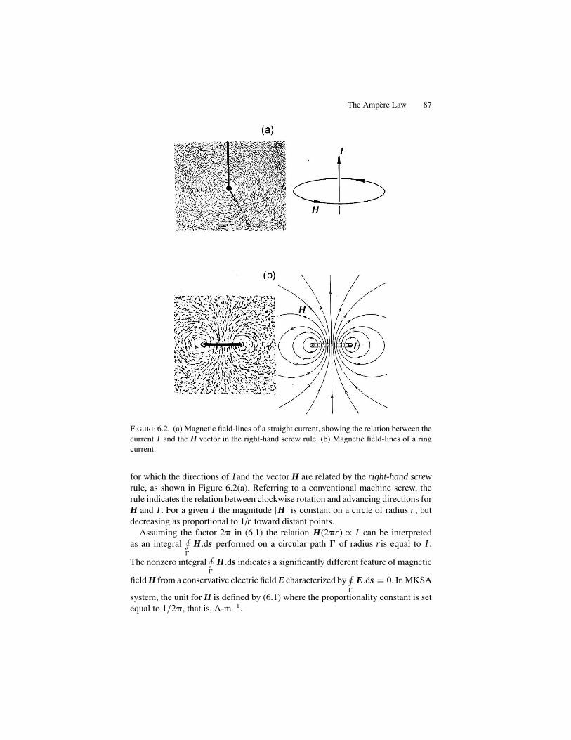
The Ampere Law 87
FIGURE 6.2. (a) Magnetic field-lines of a straight current, showing the relation between thecurrent I and the H vector in the right-hand screw rule. (b) Magnetic field-lines of a ringcurrent.
for which the directions of I and the vector H are related by the right-hand screwrule, as shown in Figure 6.2(a). Referring to a conventional machine screw, therule indicates the relation between clockwise rotation and advancing directions forH and I . For a given I the magnitude |H| is constant on a circle of radius r , butdecreasing as proportional to 1/r toward distant points.
Assuming the factor 2� in (6.1) the relation H(2�r ) ∝ I can be interpretedas an integral
∮�
H.ds performed on a circular path � of radius r is equal to I .
The nonzero integral∮�
H.ds indicates a significantly different feature of magnetic
field H from a conservative electric field E characterized by∮�
E.ds = 0. In MKSA
system, the unit for H is defined by (6.1) where the proportionality constant is setequal to 1/2�, that is, A-m−1.

88 6. The Ampere Law
The Ampere law can thus be expressed in MKS units as∮�
H.ds = I, (6.2)
which is the integral form, referring to a closed path � that encloses the current I . Itis noted that mathematically the path � does not necessarily need to be a field-linefor (6.2) to express the Ampere law. Choosing � to exclude I , equation (6.2) canbe written as
∮�
H.ds = 0, which however does not imply that H is conservative
in this case.For a magnet the magnetism originates from an entirely different microscopic
mechanism unrelated to currents. In this context, the unit of H defined aboveappears to be illogical for magnets. However, a magnetic induction effect occurswith magnets, allowing such a definition of current-related unit for fields of bothkinds. As will be discussed in the next chapter, the vector H by itself is notsufficient for characterizing a magnetic field; for the full description of this fieldthe density of field-lines is also required. Accordingly, we retain the unit A-m−1
for H.The line integral of (6.2) in the field of a straight current is shown schematically
in Figure 6.3(a) and (b).Here, the integration can be performed along radial and angular zigzag steps,
where the vector H is perpendicular and parallel to small successive displacementsdsr and ds� , respectively. Figure 6.3(a) shows a case where the closed path ofintegration � encloses the current I , whereas in Figure 6.3(b) I flows completelyoutside of �. Noted that Hr = 0, and H is signified only by the component H� ,the integral is contributed by H�(rd�) = (I /2�r )(rd�) = I d�/2�. Therefore, in
FIGURE 6.3. Calculating a line integral∮
�H.dS = 0 in a magnetic field of a straight current.
(a) The current I threaded in the path �; (b) I located outside �u

A Long Solenoid 89
the former case,
∮�
H.ds = I
2�
2�∫0
d� = I,
when I is inside �. If no current is inside, divide the path � into two parts, �1and �2,as in Figure 6.3(b), for which the subtending angles are opposite, i.e., d�1 = −d�2.Hence, we obtain ∮
�1+�2
H.ds = 0.
6.3. A Long Solenoid
As an example of the Ampere law, we consider a coiled wire wound in manyturns, which is a basic magnetic device called a solenoid serving as a practicalcomponent to control currents in electrical circuits. Figures 6.4(a) and (b) illustratethe typical pattern of the magnetic field, where a circular current in each turnproduces a magnetic field as in Figure 6.4(a), consequently providing a nearlyuniform magnetic field in a solenoid. Here, the direction of H in the coil is relatedto the current as specified by the right-hand rule. Inside a tightly wound coil ina long length, the magnetic field can be idealized as uniform in parallel with the
FIGURE 6.4. (a) Magneticfield-lines of a coil. (b) Thecurrent-field relation in a coil,an exaggerated view.
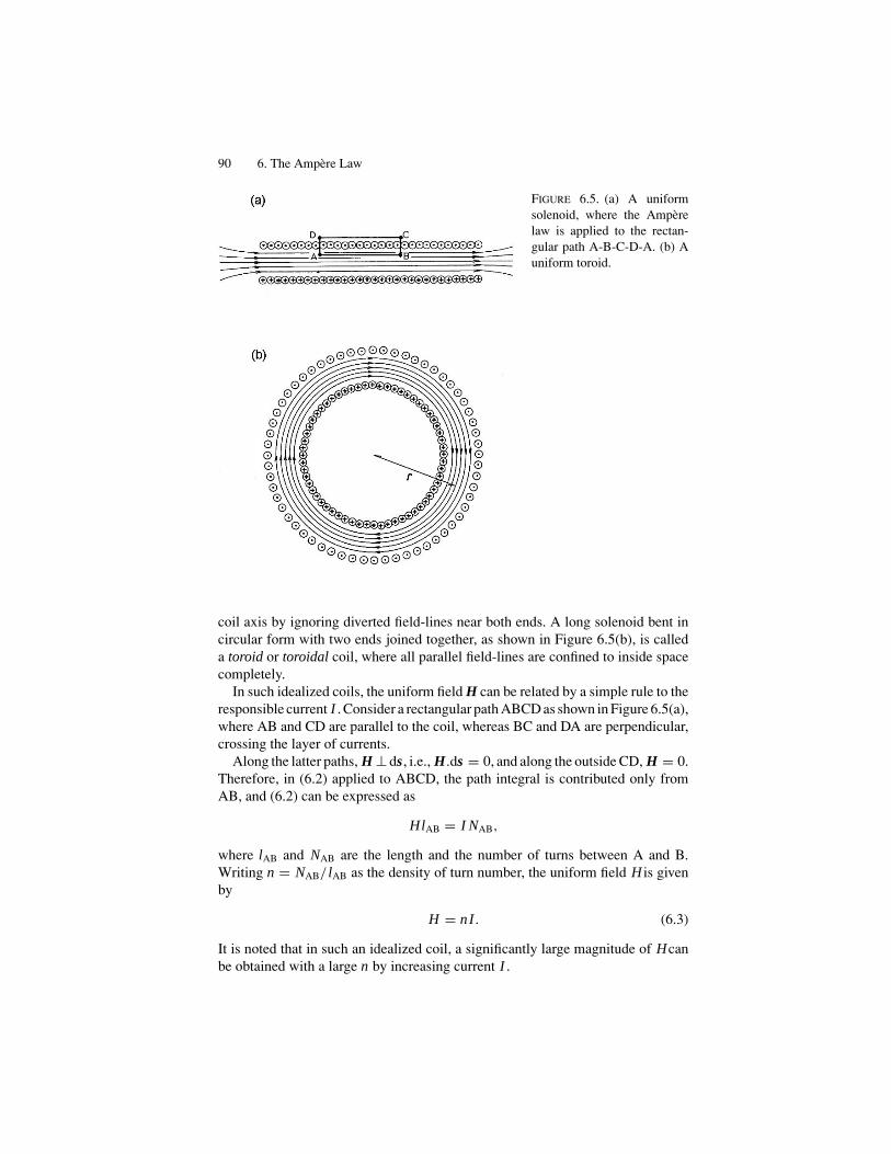
90 6. The Ampere Law
FIGURE 6.5. (a) A uniformsolenoid, where the Amperelaw is applied to the rectan-gular path A-B-C-D-A. (b) Auniform toroid.
coil axis by ignoring diverted field-lines near both ends. A long solenoid bent incircular form with two ends joined together, as shown in Figure 6.5(b), is calleda toroid or toroidal coil, where all parallel field-lines are confined to inside spacecompletely.
In such idealized coils, the uniform field H can be related by a simple rule to theresponsible current I . Consider a rectangular path ABCD as shown in Figure 6.5(a),where AB and CD are parallel to the coil, whereas BC and DA are perpendicular,crossing the layer of currents.
Along the latter paths, H ⊥ ds, i.e., H.ds = 0, and along the outside CD, H = 0.Therefore, in (6.2) applied to ABCD, the path integral is contributed only fromAB, and (6.2) can be expressed as
HlAB = I NAB,
where lAB and NAB are the length and the number of turns between A and B.Writing n = NAB/ lAB as the density of turn number, the uniform field H is givenby
H = nI. (6.3)
It is noted that in such an idealized coil, a significantly large magnitude of Hcanbe obtained with a large n by increasing current I .

Stokes’ Theorem 91
For a toroid of the turn number N , shown in Figure 6.5(b), we can write arelation similar to (6.3) if the radius r is sufficiently large. In this case, H canbe considered as constant circularly, for which the Ampere law can be writ-ten as H (2�r ) = NI, and hence H = N I/2�r . In such a solenoid or toroid,there is a large H as given by a large nI or NI, respectively, similar to the re-lation between the electric flux density D and the condensed charges ±� in acapacitor.
6.4. Stokes’ Theorem
Macroscopic electric currents can be attributed to moving charged particles in aconductor. Although invisible, such a current is evidenced by heat generated in aconducting material as well as by the magnetic field produced by the motion. Infact, it was Rowland (1848) who demonstrated magnetically that a charged bodyin motion is equivalent to a current (See Section 6.7). Effects of a current suchas heat, magnetic field, and chemical reactions in electrolysis were regarded asvisual evidence for an invisible current. Conduction current can thus be identifiedgeometrically along with a curve of the wire, which is, however, not the same formoving charge carriers .
The current I is defined by the total charge passing through the area S acrossthe passage per second, where the density at a local point is often significant.Namely, I = ∫
Sj .dS, where j represents the current density on differential area dS
and determines the integral∮�
H.ds for the magnetic field H along the rim � of the
area S. However, to deal with local properties, we need to convert the Ampere lawinto a differential form. Stokes’ theorem is required for such a conversion, as wenow explain.
In this section, we derive Stokes’ theorem in rectangular coordinates, for sim-plicity, then in curvilinear coordinates, as discussed in the next section. First, wewrite
∮�
H.ds =∮�
(Hx dx + Hydy + Hzdz
)
= 1
2
[ ∮Cz
(Hx dx + Hydy
) +∮Cx
(Hydy + Hzdz
) +∮Cy
(Hzdz + Hx dx)
](i)
where terms on the right can be integrated along closed paths Cz, Cx , and Cy
that are projections of the curve C onto planes xy, yz, and zx, respectively. Figure6.6 shows Cz on the xy-plane, for example, where the integral can be calculatedapproximately as the sum of integrals over such closed square paths marked asabcda. In fact, both clockwise and counter clockwise integrals give the sameresults, making 1 the front factor of the square brackets in (i), instead of 1
2 , if we
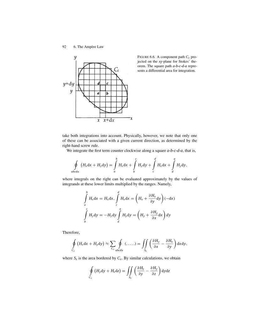
92 6. The Ampere Law
FIGURE 6.6. A component path Cz pro-jected on the xy-plane for Stokes’ the-orem. The square path a-b-c-d-a repre-sents a differential area for integration.
take both integrations into account. Physically, however, we note that only oneof these can be associated with a given current direction, as determined by theright-hand screw rule.
We integrate the first term counter clockwise along a square a-b-c-d-a, that is,
∮abcda
(Hx dx + Hydy
) =b∫
a
Hx dx +c∫
b
Hydy +d∫
c
Hx dx +a∫
d
Hydy,
where integrals on the right can be evaluated approximately by the values ofintegrands at these lower limits multiplied by the ranges. Namely,
b∫a
Hx dx = Hx dx,
d∫c
Hx dx =(
Hx + ∂ Hx
∂ydy
)(−dx)
c∫b
Hydy = −Hydy
a∫d
Hydy =(
Hy + ∂ Hy
∂xdx
)dy
Therefore,∮Cz
(Hx dx + Hydy
) ≈∑Cz
∮abcda
(. . . . .) =∫∫
Sz
(∂ Hy
∂x− ∂ Hx
∂y
)dxdy,
where Sz is the area bordered by Cz . By similar calculations, we obtain
∮Cx
(Hydy + Hzdz
) =∫∫
Sx
(∂ Hz
∂y− ∂ Hy
∂z
)dydz
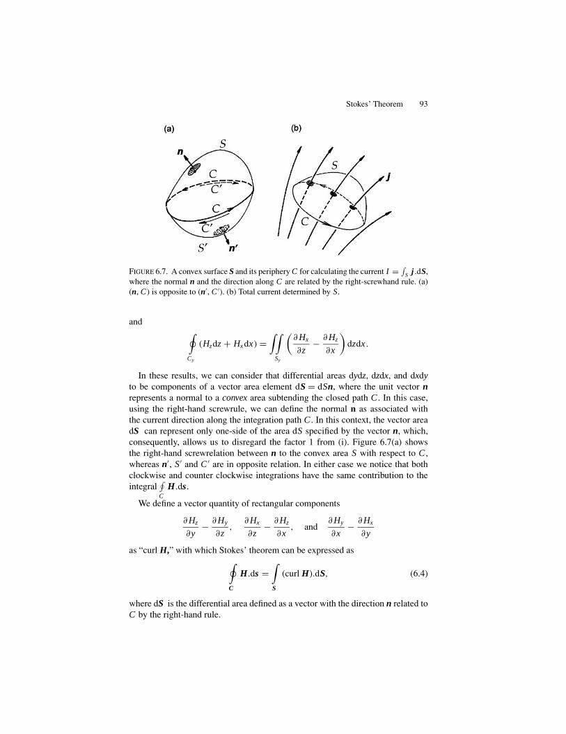
Stokes’ Theorem 93
FIGURE 6.7. A convex surface S and its periphery C for calculating the current I = ∫S j .dS,
where the normal n and the direction along C are related by the right-screwhand rule. (a)(n, C) is opposite to (n′, C ′). (b) Total current determined by S.
and ∮Cy
(Hzdz + Hx dx) =∫∫
Sy
(∂ Hx
∂z− ∂ Hz
∂x
)dzdx .
In these results, we can consider that differential areas dydz, dzdx, and dxdyto be components of a vector area element dS = dSn, where the unit vector nrepresents a normal to a convex area subtending the closed path C . In this case,using the right-hand screwrule, we can define the normal n as associated withthe current direction along the integration path C . In this context, the vector areadS can represent only one-side of the area dS specified by the vector n, which,consequently, allows us to disregard the factor 1 from (i). Figure 6.7(a) showsthe right-hand screwrelation between n to the convex area S with respect to C ,whereas n′, S′ and C ′ are in opposite relation. In either case we notice that bothclockwise and counter clockwise integrations have the same contribution to theintegral
∮C
H.ds.
We define a vector quantity of rectangular components
∂ Hz
∂y− ∂ Hy
∂z,
∂ Hx
∂z− ∂ Hz
∂x, and
∂ Hy
∂x− ∂ Hx
∂y
as “curl H,” with which Stokes’ theorem can be expressed as∮C
H.ds =∫S
(curl H).dS, (6.4)
where dS is the differential area defined as a vector with the direction n related toC by the right-hand rule.
94 6. The Ampere Law
It is noted that curl H is identical to the cross-product between ∇ and H, andwritten as
curl H = ∇ × H =
∣∣∣∣∣∣∣∣∣
i j k
∂
∂x
∂
∂y
∂
∂z
Hx Hy Hz
∣∣∣∣∣∣∣∣∣, (6.5)
where i, j, and k are unit vectors along the x-, y-, and z-axes, respectively.
6.5. Curvilinear Coordinates (2)
In Section 6.4, we expressed the differential operator curl H in rectangular co-ordinates. For practical applications, however, it is often necessary to write it incurvilinear coordinates, as we discussed for other operators, e.g., div and ∇2, inSection 4.3. However, the operator curl ≡ ∇× is a little more complex, and hencewe elaborate on it in this section for future applications.
The rectangular coordinates x , y, and z can be expressed as functions of thecorresponding curvilinear coordinates u1, u2, and u3. We can therefore define thefollowing three vectors defined as the basic vectors for the curvilinear space. Thatis,
a1 = ∂r∂u1
= ∂x
∂u1i + ∂y
∂u1j + ∂z
∂u1k = h1e1,
a2 = ∂r∂u2
= ∂x
∂u2i + ∂y
∂u2j + ∂z
∂u2k = h2e2, (6.6)
a3 = ∂r∂u3
= ∂x
∂u3i + ∂y
∂u3j + ∂z
∂u3k = h3e3,
where
h21 =
(∂x
∂u1
)2
+(
∂y
∂u1
)2
+(
∂z
∂u1
)2
, h22 =
(∂x
∂u2
)2
+(
∂y
∂u2
)2
+(
∂z
∂u2
)2
,
h23 =
(∂x
∂u3
)2
+(
∂y
∂u3
)2
+(
∂z
∂u3
)2
.
With these expressions a differential displacement dr can be written as
dr = ∂r∂u1
du1 + ∂r∂u2
du2 + ∂r∂u3
du3 = (h1du1) e1 + (h2du2) e2 + (h3du3) e3,
(6.7)
indicating that (h1du1, h2du2, h3du3) are curvilinear components of dr.
Curvilinear Coordinates (2) 95
For a gradient of a scalar function V , we can write that
∂V
∂u1= ∂V
∂x
∂x
∂u1+ ∂V
∂y
∂y
∂u1+ ∂V
∂z
∂z
∂u1= h1e1 · ∇V ,
∂V
∂u2= h2e2 · ∇V and
∂V
∂u3= h3e3 · ∇V,
where ∇V =(
∂V
∂x,∂V
∂y,∂V
∂z
)consistent with (4.6).
To obtain the curvilinear expression for the operator ∇×, we define the recip-rocal vectors a1, a2 and a3, corresponding to a1, a2, and a3, respectively. Theseare related as
a1 · a1 = a2 · a2 = a3 · a3 = 1, and a1 = 1
�(a2×a3),
a2 = 1
�(a3×a1), a3 = 1
�(a2×a3),
where � = (a1a2a3) = h1h2h3(e1e2e3) = h1h2h3 is the volume of the reciprocalunit cell. It is noted that the gradient operator ∇, therefore, has components in thereciprocal space that are given by
∇1 = a1∂
∂u1, ∇2 = a2
∂
∂u2, and ∇3 = a3
∂
∂u3. (6.8)
Now, for an arbitrary vector F, we derive an expression for curl F = ∇ × F.Writing
F = F1a1 + F2a2 + F3a3,
(∇×F)i = ∂ Fk
∂uj(aj×ak) + ∂ Fj
∂uk(ak×aj) =
(∂ Fk
∂uj− ∂ Fj
∂uk
)(aj×ak)
= 1
�
(∂ Fk
∂uj− ∂ Fj
∂uk
)ai,
and hence
curl F = 1
�
∣∣∣∣∣∣∣∣∣
a1 a2 a3
∂
∂u1
∂
∂u2
∂
∂u3
F1 F2 F3
∣∣∣∣∣∣∣∣∣, (6.9a)
or
curl F = 1
h1h2h3
∣∣∣∣∣∣∣∣∣
h1e1 h2e2 h3e3
∂
∂u1
∂
∂u2
∂
∂u3
h1 F1 h2 F2 h3 F3
∣∣∣∣∣∣∣∣∣. (6.9b)

96 6. The Ampere Law
With polar coordinates, (6.9b) can be written specifically as
curl F(r, �, �) = 1
r2 sin �
∣∣∣∣∣∣∣∣∣
er re� r sin �e�
∂
∂u1
∂
∂u2
∂
∂u3
Fr r F� r sin �F�
∣∣∣∣∣∣∣∣∣(6.10)
6.6. The Ampere Law in Differential Form
A vortex-like magnetic field is produced by an electric current as described bythe Ampere law, where current directions are related by the right-hand screw rule.The clockwise direction of the H vector and the related current I correspond torotating and advancing directions of a right-hand screw. In this context, the currentj passing through a closed field-line of H can be expressed as
I =∫S
j .dS,
where S is a convex surface bordered by a closed curve C , as illustrated in Figure6.7(b).
Therefore, the Ampere law (6.2), if we consider �go be such a closed field-lineC , can be written as ∮
C
H.ds =∫S
j .dS. (6.11)
Using Stokes’ theorem (6.4), the left side can be replaced by a surface integral,and therefore ∫
S
(curl H) .dS =∫S
j .dS,
and we obtain
curl H(r ) = j(r ) (6.12)
at a point r, which is the Ampere law in differential form.Equation (6.12) is the law that can be applied locally to an arbitrary position
r in the field. Although H = 0 at a position r where j = 0, there is a point r′ inthe field where H �= 0, even if j(r′) = 0. In this case, curl H(r ′) = 0 correspondsto the integral law
∮�
H.ds = 0, where � is chosen arbitrarily by enclosing no
currents. Such a magnetic field H appears to be conservative in this region, wherea magnetic scalar potential can be defined from H(r ′) = −∇m(r ′). However, inthe Ampere law (6.2) the curve � must be a field-line C encircling the currentj. Along an arbitrary path �, physically neither a unit magnetic charge could befound to move, as will be discussed in Chapter 8, and hence the field of H is not
The Ampere Law in Differential Form 97
conservative. Nevertheless, the magnetic potential Vm(r ′) is a useful mathematicalconcept for calculation, called a pseudo-potential.
As an example, we consider a long cylindrical conductor of circular cross-sectional area of radius a, which extends along the z-axis. Assuming that a currentI is flowing steadily along the conductor, we calculate the magnetic field, using firstthe Ampere law in integral form,
∮C H · ds = I . We can use cylindrical coordinates
r , �, z, referring z to the cylinder axis. At a point for r > a, a circle C of radius rencloses the entire current I inside of �, whereas for r < a, only I (r /a)2 needs tobe considered for the integral on C . Further, considering that only the componentH� is significant, we can write that H�(2�r ) = I and H�(2�r ) = I (r /a)2 for r > aand for r < a, respectively, and obtain
H� = I
2�r(for r > a) and H� = I r
2�a2(for r < a).
The differential equation (6.12) offers a more accurate analysis for obtainingthe correct solution. In terms of the components, (6.12) can be expressed as
1
r
∂ Hz
∂�− ∂ H�
∂z= 0,
∂ Hr
∂z− ∂ Hz
∂r= 0, and
1
r
∂(r H�
)∂r
− 1
r
∂ Hr
∂�= j.
As the field components should be independent of � and z by symmetry, onlythe derivatives with respect to r are significant in these equations. From the second
relation, we obtain∂ Hz
∂r= 0, and hence Hz = constant, which eventually leads
us to a constant Hr , independent of the current. However, this value cannot bedetermined by (6.11) only, unless the problem is supplemented by the relation divH = 0.
From the third equation, we have
1
r
d(r H�
)dr
= j, where j = 0 (for r > a) and j = I
�a2(for r < a),
which can be integrated as
H� = c1
r(for r > a) and H� = I r
2�a2+ c2
r(for r < a),
where c1 = I /4� and c2 = 0 were determined by the conditions at r = a andr = ∞.
The above example shows clearly that the Ampere law for the H vector is notsufficient to determine the magnetic field of a current, hence we require another lawsuch as div H = 0 to complete the description. It is notable from the relation H� =I/2�r for r > a we can define the scalar potential with H = −∇Vm, namely,
Vm = − I
2�� satisfying
Hr = −∂Vm
∂r= 0 and H� = −1
r
∂Vm
∂�= I
2�r.
Here, it is noted that Hr = 0 is originated from div H = 0, regardless of I .
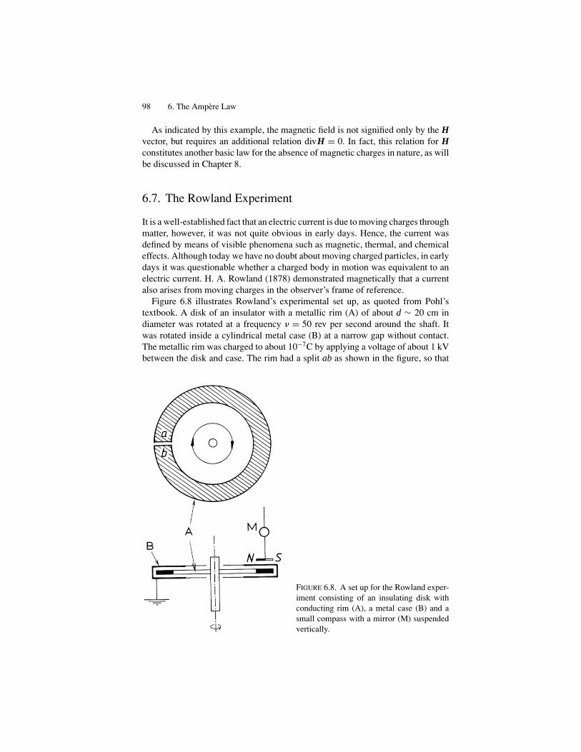
98 6. The Ampere Law
As indicated by this example, the magnetic field is not signified only by the Hvector, but requires an additional relation divH = 0. In fact, this relation for Hconstitutes another basic law for the absence of magnetic charges in nature, as willbe discussed in Chapter 8.
6.7. The Rowland Experiment
It is a well-established fact that an electric current is due to moving charges throughmatter, however, it was not quite obvious in early days. Hence, the current wasdefined by means of visible phenomena such as magnetic, thermal, and chemicaleffects. Although today we have no doubt about moving charged particles, in earlydays it was questionable whether a charged body in motion was equivalent to anelectric current. H. A. Rowland (1878) demonstrated magnetically that a currentalso arises from moving charges in the observer’s frame of reference.
Figure 6.8 illustrates Rowland’s experimental set up, as quoted from Pohl’stextbook. A disk of an insulator with a metallic rim (A) of about d ∼ 20 cm indiameter was rotated at a frequency � = 50 rev per second around the shaft. Itwas rotated inside a cylindrical metal case (B) at a narrow gap without contact.The metallic rim was charged to about 10−7C by applying a voltage of about 1 kVbetween the disk and case. The rim had a split ab as shown in the figure, so that
FIGURE 6.8. A set up for the Rowland exper-iment consisting of an insulating disk withconducting rim (A), a metal case (B) and asmall compass with a mirror (M) suspendedvertically.
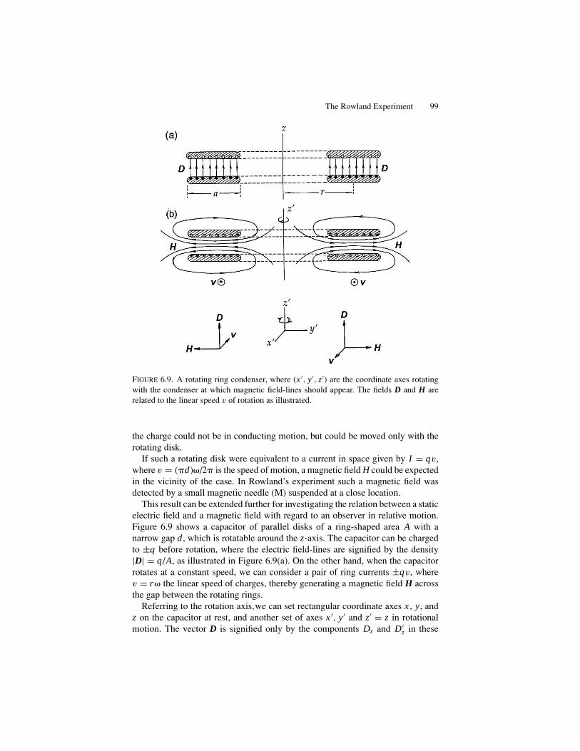
The Rowland Experiment 99
FIGURE 6.9. A rotating ring condenser, where (x ′, y′, z′) are the coordinate axes rotatingwith the condenser at which magnetic field-lines should appear. The fields D and H arerelated to the linear speed v of rotation as illustrated.
the charge could not be in conducting motion, but could be moved only with therotating disk.
If such a rotating disk were equivalent to a current in space given by I = qv,where v = (�d)�/2� is the speed of motion, a magnetic field H could be expectedin the vicinity of the case. In Rowland’s experiment such a magnetic field wasdetected by a small magnetic needle (M) suspended at a close location.
This result can be extended further for investigating the relation between a staticelectric field and a magnetic field with regard to an observer in relative motion.Figure 6.9 shows a capacitor of parallel disks of a ring-shaped area A with anarrow gap d , which is rotatable around the z-axis. The capacitor can be chargedto ±q before rotation, where the electric field-lines are signified by the density|D| = q/A, as illustrated in Figure 6.9(a). On the other hand, when the capacitorrotates at a constant speed, we can consider a pair of ring currents ±qv, wherev = r� the linear speed of charges, thereby generating a magnetic field H acrossthe gap between the rotating rings.
Referring to the rotation axis,we can set rectangular coordinate axes x , y, andz on the capacitor at rest, and another set of axes x ′, y′ and z′ = z in rotationalmotion. The vector D is signified only by the components Dz and D′
z in these
100 6. The Ampere Law
systems, although Dz ≈ D′z unless v is close to the speed of light c, according to
the relativity theory. However, a stationary observer should recognize a magneticfield between the disks in the radial direction y′, as related to D′
z and v, dependingon how v compares with c. As illustrated in the Figure 6.9(b), these factors arerelated by H ′
y ∝ v × D′z , as consistent with Ampere’s law, and such a field H ′
zshould be detectable by a stationary observer, in principle. In contrast, an observermoving with the disks should detect only Dz . Such an attempt may remain athought experiment, but it gives insight into the relativity theory in relation todynamic electromagnetism.
7Magnetic Induction
7.1. Laws of Magnetic Induction
The magnetic field is a property of the space that surrounds an electric currentand a magnet. In early physics powdered iron was used to visualize its geometriccharacter, and the distributed field intensities were studied with a compass needle.However, such observations were hardly subject to systematic investigations, untila coiled wire became available for studying a uniform magnetic field at a measur-able intensity. Indicated by a ripple pattern of iron particles, the field-lines revealedthe distribution in space, which were recognized as significant for describing thenature of a magnetic field. Faraday (1832) made a number of sketches of field-linesemphasizing the significance of a distributed pattern, and he discussed the fieldwith the concept of flux of field-lines. In fact, in the previous chapters we used hisidea for electric fields for which electric charges on conductors were responsible.For a magnetic field, in contrast, we cannot argue further using electric analogiesbecause magnetic charges are absent in nature. Nevertheless, with the concept offlux Faraday described the induction effect in magnetic fields, which lead him toestablish the fundamental laws of electromagnetism. Owing to Faraday’s discov-ery, the flux of magnetic field-lines, as determined by induced voltages, allows aquantitative description of the magnetic field with no responsible magnetic charges.
7.1.1. The Faraday Law
Figure 7.1 shows a basic set up to demonstrate the magnetic induction effect. Thecoil L in Figure 7.1(a) produces a magnetic field (as sketched in Figure 6.4), wherethe field-lines are in near parallel inside L , when activated by a steady current. Asmaller coil Lo connected with a galvanometer G can be moved to and from L todetect an induction current. Figure 7.1(b) shows another set up with a permanentmagnet, where a similar induction effect can be observed by moving Lo. Aninduction current in Lo flows as related to the flux through the cross-sectional areaS, and hence the flux can be defined in terms of an observed induction current. Amodern version of Lo with a connected circuit, called a search coil and fluxmeter,is a basic device for measuring the magnetic field.
101

102 7. Magnetic Induction
FIGURE 7.1. (a) Magnetic induction between twocoils L and Lo. Induction between a magnet and asearch coil Lo.
When Lo is moved against L , an induced current I can be observed on G,depending on the electrical resistance of Lo, for which the induced emf (Vemf) isconsidered primarily responsible. The emf voltage varies as a function of the timefor the relative motion between Lo and L or the magnet, exhibiting a pulse-shapedpeak, as sketched in Figure 7.2, which is higher the faster the movement. Theobserved Vemf depends on other factors of Lo, such as the area S, turn number N,and the closest position. However, most significant is that the voltage pulse definedby U = ∫ ∞
0 Vemf (t) dt is independent of the speed, which is therefore considereda variable for expressing the magnetic flux.
The number of field-lines, or the flux, is determined by �� = ∫S BdS = BS per
one turn in Lo if the field is uniform, which can then be described by an observedpulse U /N, where N is the number of turns in the search coil Lo. By equating�� to U /N, the flux density B can be defined as B = U /NS. In this definitionthe unit of B is given by V-sec/m2 in the MKSA system, a unit called the “tesla.”The traditional CGS unit “gauss” is still in use; the conversion to tesla is 1 tesla
FIGURE 7.2. Examples of inductionpulses. a and b correspond to fast andslow movement of a search coil, respec-tively. Empirically, these areas
∫ ∞0 V dt
are identical.

Laws of Magnetic Induction 103
= 104gauss. Also, the flux �� = BS is measured in the practical unit “weber,”which is the same as the voltage pulse in V-sec, and accordingly tesla = weber/m2.
The quantity �� represents the flux of field-lines that is picked up by one turnof a search coil when inserted in the magnetic field. At a given position of Lo, theFaraday law can then be expressed as
��(t) =∫ t
0|Vemf (t)| dt or
d�
dt= |Vemf (t)| (7.1)
and, hence, the observed |Vemf(t)| represents a changing rate of the flux throughthe area S of a search coil. It is noted that the formula (7.1) between the magnitudeof Vemf(t) and d�/dt is not exactly correct for magnetic induction phenomenasince the direction of Vemf(t) is not specified. Nevertheless, (7.1) indicates that themagnetic induction is signified by an induced voltage pulse in a moving coil, andis called the Faraday law.
7.1.2. The Lenz Law
Lenz also studied magnetic induction and published his interpretation in 1834.Lenz revised the Faraday law by attaching the correct sign to the induced voltage;the revised law is called the Lenz law. At his time, electronic motion in metalswas not a familiar concept, so that induced emf was not recognized as originatingfrom an electronic mechanism. Nevertheless, Lenz considered a mutual interactionbetween coils, referring to Newton’s action-reaction principle.
The induction current flowing in a coil generates heat in Lo, indicating that achange �� in the main coil L can be attributed to a mutual interaction energybetween Lo and L . If so, it is logical to consider the reaction −�� of Lo to thechange �� as originating from such a mutual interaction, and hence the inductioncurrent can flow as the reaction −��. In this way (7.1) can be revised as
−�� =∫ t
0|Vemf (t)| dt or − d�
dt= |Vemf (t)| , (7.2)
which is the Faraday-Lenz formula. Originally Lenz stated that the inductioncurrent should flow in such a direction as to oppose the change ��, which canbe precisely expressed in the revised formula (7.2). Figure 7.3 shows the relationbetween positive directions for d�/dt and Vemf = RI, where R is the resistance ofLo and the detector, a resistance that is described by the left-hand screw rule.
7.1.3. Magnetic Field Vectors
In the above, we considered a search coil Lo of cross-sectional area S, placedperpendicular to the field direction, in which the flux was defined as �� = BS.Considering S as a vector S = Sn, where n is the unit vector to the area, thequantity B can logically be regarded as a vector B, signifying the direction offield-lines. In this definition, |B| cos �, where cos � = (B.n)/B, represents thedensity of field-lines measured as the induced voltage pulse U /N of Lo.

104 7. Magnetic Induction
FIGURE 7.3. Magnetic induction. (a) Induction currentI as related toB, (b) dynamic electric field E relatedto B.
On the other hand, the magnetic field in the coil L was expressed by another fieldvector H, as stated by the Ampere law. The magnitude is given by |H| = nI if Lis sufficiently long, and the direction of H is tangential to the field-line. With thesetwo descriptions combined, the region of “intense” field can be specified by a largevalue of |B|, whereas the direction of field-lines can be specified by the vector H.
The uniform field in a long solenoid can be shown by parallel field-lines thatare evenly distributed, where the vectors B and H are parallel. For such an emptysolenoid, we can write a proportionality relation
B = �o H, (7.3)
where �o is an empirical constant. The value of �o can be determined experimen-tally from the relation U/N S = �onI , and is known as
�o = 1.256 × 10−6 = 4� × 10−7 V sec/A-m.
Considered for representing empty space, like dielectric parameter εo in electro-statics, the constant �o is required for all calculations with MKSA units.
7.2. Differential Law of Induction and the DynamicElectric Field
In a magnetic field, field-lines are described by two vectors H and B expressingtheir intensities and distribution, respectively. In a uniform field inside a longsolenoid, the two vectors represent parallel field-lines at a constant density over
Differential Law of Induction and the Dynamic Electric Field 105
almost entire volume, where we have the relation B = �o H , and the flux is simplyexpressed by � = BS. In a more general field the distributed flux should be relatedwith respect to a closed area S for counting the number of lines within its peripheralcurve C , as expressed by � = ∫
S B.dSGenerally, such a flux is a function of time t , as indicated by induction exper-
iments. According to the Faraday-Lenz law, an emf (Vemf) is induced in a coilby changing magnetic flux � through the sectional area S. Such an area S fordefining � is essential for Vemf; on the other hand, due to the emerging potentialdifference −V (t) = Vemf, the corresponding electric field E(t)must be consideredin the coiled wire, driving charge carriers in motion. In this context, the Faradaylaw can be re-expressed as
− d
dt
∫S
B.dS =∮C
E.ds, (7.4)
which is the Faraday-Lenz formula in integral form. Such an electric field E(t) in(7.4), called the dynamic electric field, has been best substantiated in the betatronaccelerator, where particles of charge e are accelerated by a force eE(t).
Using the Stokes theorem, we convert the integral on the right side of (7.4) toa surface integral, i.e.,
∮C
E.ds = ∫S
curl E.dS, and hence the equation (7.4) can be
reduced to a differential form, that is,
−∂ B
∂t= curl E. (7.5)
Such a dynamic electric field is not conservative because curl E �= 0, as indicated
by (7.5), or∮C
E.ds �= 0, for∂ B∂t
�= 0. If a small charge qis brought into such a
field E, a characteristic force F = qE can be detected to verify the effect. Suchforces should act on charged particles and mobile charge carriers in matter as well,so that a moving conductor in a magnetic field should be subjected to such a forcedue to the induction effect, which is therefore called a magnetic force.
Figure 7.4 illustrates an example of a conducting wire that is moved in a uniformmagnetic field against a magnetic force. Consider that B is normal to the page, anda pair of long parallel wires is placed perpendicular to B, to which a galvanometerG connected. A metal rod ab with an insulating handle P slides along the wires tothe right or to the left. The rod and a portion of the wires form a closed loop alongwhich an induction current can flow when the rod is moved. Denoting the lengthbetween contact points a and b by l, and the sliding distance of the rod as x fromthe initial position marked o-o, the magnetic flux in the area swept by the rod isgiven by � = Blx . When ab slides at a speed v = dx/dt , the Faraday-Lenz lawdescribes the induced emf voltage
Vemf = −d�
dt= −Blv,
giving a potential difference V (t) = −Vemf = Blv on the moving rod.
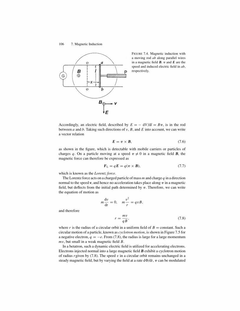
106 7. Magnetic Induction
FIGURE 7.4. Magnetic induction witha moving rod ab along parallel wiresin a magnetic field B. v and E are thespeed and induced electric field in ab,respectively.
Accordingly, an electric field, described by E = − dV /dl = Bv , is in the rodbetween a and b. Taking such directions of v, B, and E into account, we can writea vector relation
E = v × B, (7.6)
as shown in the figure, which is detectable with mobile carriers or particles ofcharges q . On a particle moving at a speed v �= 0 in a magnetic field B, themagnetic force can therefore be expressed as
FL = q E = q(v × B), (7.7)
which is known as the Lorentz force.The Lorentz force acts on a charged particle of mass m and charge q in a direction
normal to the speed v, and hence no acceleration takes place along v in a magneticfield, but deflects from the initial path determined by v . Therefore, we can writethe equation of motion as
mdv
dt= 0, m
v2
r= qvB,
and therefore
r = mv
q B, (7.8)
where r is the radius of a circular orbit in a uniform field of B = constant. Such acircular motion of a particle, known as cyclotron motion, is shown in Figure 7.5 fora negative electron, q = −e. From (7.8), the radius is large for a large momentummv, but small in a weak magnetic field B.
In a betatron, such a dynamic electric field is utilized for accelerating electrons.Electrons injected normal into a large magnetic field B exhibit a cyclotron motionof radius rgiven by (7.8). The speed v in a circular orbit remains unchanged in asteady magnetic field, but by varying the field at a rate d�/dt , v can be modulated

Differential Law of Induction and the Dynamic Electric Field 107
FIGURE 7.5. An electron in a uniform magneticfield B. The centripetal force F = −e(v×B) isresponsible for the cyclotron motion.
by the dynamic electric emf voltage arising from d�/dt . The circular motion andvarying field can be synchronized to accelerate electrons. An average rate of 1weber/10−3-s is technically quite feasible, giving rise to an induced emf of theorder of 1 kV, which can accelerate electrons when the cyclotron motion andd�/dt are in phase.
Equation (7.7) can also be expressed for a macroscopic magnetic force on acurrent flowing in a magnetic field. Consider that a conducting wire of cross-sectional area A and the length l is exposed to a uniform field B. The current onsuch a wire is given by I = jA, where j = nqv, and n = N/(Al ) are the currentdensity and the number density of carrier particles, respectively. Hence, qv =I/n A = (I/N)l. The Lorentz force FL given by (7.7) acts on all particles in thecurrent, so that the macroscopic force is given by NFL = F. Hence, the force onthe conduction wire can be expressed as
F = I (l × B), (7.9)
where the vector l indicates the direction of the current I specified by the wire.Figure 7.6 illustrates the relation (7.9).
Because of the induction effect, an amount of work is required for a conductingbody to move in a magnetic field, resulting in an induced current and heat inthe coil. Such a process can be described by the law of energy conservation; the
FIGURE 7.6. A magnetic force F on a straightcurrent I in a uniform magnetic field B(B⊥ I ).

108 7. Magnetic Induction
input power to move against the magnetic force is equal to the heat producedin the output. Namely, Pin = −F.v = −IlBv = (Vemf/R)lBv , where Vemf = Blvand R is the electrical resistance of the conductor. Therefore, we obtain Pin =(Blv )2/R = V 2
emf/R = Pout.We discussed a moving rod in the above example, but the induction can generally
take place in any conducting body in a magnetic field, where the induction causesa distributed current called an eddy current. For example, in a simple pendulum ofa metallic bob in a magnetic field, the amplitude is decreased with time, as inducededdy currents generate heat in the bob.
7.3. Magnetic Moments
A magnetic force on a current given by (7.9) has numerous engineering applica-tions: alternating current (AC) generators, AC and DC motors, metering devices,and many others. A coiled wire in compact size is suitable for the rotation in alimited space between magnetic poles, converting electric energies to mechanicalones via a magnetic induction effect. Such a rotating coil in a magnetic field maybe described conveniently in terms of a magnetic moment.
Although rectangular and circular coils are used in many practical applications,a coil in arbitrary shape can be discussed for a general description. As we dis-cussed for the Stokes theorem, the area of a given coil can be divided into manysmall rectangular areas as shown in Figure 6.6, where each one is regarded asan elementary rectangular coil. Assuming that all of these currents flow aroundsmall coils in the same direction with an equal magnitude, their integrated resultis equivalent to a current around the peripheral rim. Therefore, for a theoreticalargument it is convenient to consider a small rectangular coil in order to calculatethe resultant induction in a given coil. Nevertheless, a coil in rectangular shape issuitable for many practical designs.
Figure 7.7(a) shows a rectangular coil that can be rotated around the axis asindicated. On the four edges currents flow in different directions in the magneticfield B, and hence four different forces, F1, F2, F3, and F4, determined by (7.9),should be considered together, as shown in the figure. It is noted that F2 andF4 are equal in magnitude but go in opposite directions parallel to the axis, thuscausing no effect to the rigid coil. In contrast, F1 and F3 are equal and opposite,being exerted on different parts of the coil in perpendicular directions to the axis.Consequently, a torque or a couple of forces acts on the coil. As |F1| = |F3| = I bBin this case, the torque can be expressed as � = I bB × a sin �, where b and a areedge lengths, and � is the angle between B and the normal n to the rectangular areaof the coil, as indicated in Figures 7.7(a) and (b). Considering the area ab = S asa vector S = Sn, where the direction of n and the current direction are related bythe right-hand rule, the torque is written as a vector
� = I S × B = pm × H, where pm = �o I S. (7.10)
Here, the vector pm is called the magnetic moment of the coil. However, the
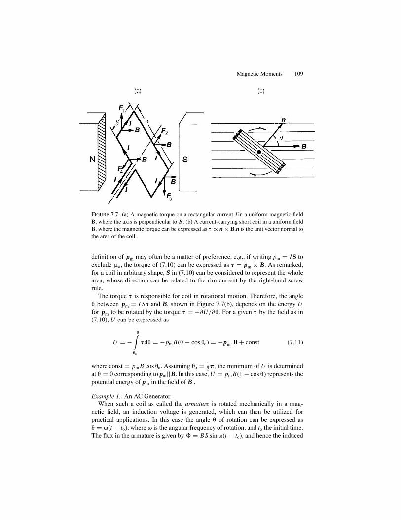
Magnetic Moments 109
FIGURE 7.7. (a) A magnetic torque on a rectangular current I in a uniform magnetic fieldB, where the axis is perpendicular to B. (b) A current-carrying short coil in a uniform fieldB, where the magnetic torque can be expressed as � ∝ n × B.n is the unit vector normal tothe area of the coil.
definition of pm may often be a matter of preference, e.g., if writing pm = I S toexclude �o, the torque of (7.10) can be expressed as � = pm × B. As remarked,for a coil in arbitrary shape, S in (7.10) can be considered to represent the wholearea, whose direction can be related to the rim current by the right-hand screwrule.
The torque � is responsible for coil in rotational motion. Therefore, the angle� between pm = I Sn and B, shown in Figure 7.7(b), depends on the energy Ufor pm to be rotated by the torque � = −∂U/∂�. For a given � by the field as in(7.10), U can be expressed as
U = −�∫
�o
�d� = −pm B(� − cos �o) = −pm.B + const (7.11)
where const = pm B cos �o. Assuming �o = 12 �, the minimum of U is determined
at � = 0 corresponding to pm||B. In this case, U = pm B(1 − cos �) represents thepotential energy of pm in the field of B .
Example 1. An AC Generator.When such a coil as called the armature is rotated mechanically in a mag-
netic field, an induction voltage is generated, which can then be utilized forpractical applications. In this case the angle � of rotation can be expressed as� = �(t − to), where � is the angular frequency of rotation, and to the initial time.The flux in the armature is given by � = BS sin �(t − to), and hence the induced
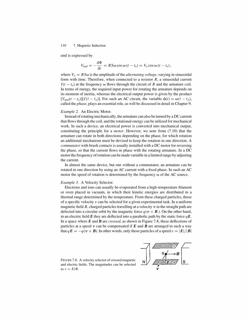
110 7. Magnetic Induction
emf is expressed by
Vemf = −d�
dt= BS� cos � (t − to) = Vo cos � (t − to) ,
where Vo = BS� is the amplitude of the alternating voltage, varying in sinusoidalform with time. Therefore, when connected to a resistor R, a sinusoidal currentI (t − to) at the frequency � flows through the circuit of R and the armature coil.In terms of energy, the required input power for rotating the armature depends onits moment of inertia, whereas the electrical output power is given by the product[Vemf(t − to)][I (t − to)]. For such an AC circuit, the variable �(t) = �(t − to),called the phase, plays an essential role, as will be discussed in detail in Chapter 9.
Example 2. An Electric Motor.Instead of rotating mechanically, the armature can also be turned by a DC current
that flows through the coil, and the rotational energy can be utilized for mechanicalwork. In such a device, an electrical power is converted into mechanical output,constituting the principle for a motor. However, we note from (7.10) that thearmature can rotate in both directions depending on the phase, for which rotationan additional mechanism must be devised to keep the rotation in one direction. Acommutator with brush contacts is usually installed with a DC motor for reversingthe phase, so that the current flows in phase with the rotating armature. In a DCmotor the frequency of rotation can be made variable in a limited range by adjustingthe current.
In almost the same device, but one without a commutator, an armature can berotated in one direction by using an AC current with a fixed phase. In such an ACmotor the speed of rotation is determined by the frequency � of the AC source.
Example 3. A Velocity Selector.Electrons and ions can usually be evaporated from a high-temperature filament
or oven placed in vacuum, in which their kinetic energies are distributed in athermal range determined by the temperature. From these charged particles, thoseof a specific velocity v can be selected for a given experimental task. In a uniformmagnetic field B, charged particles travelling at a velocity v in the straight path aredefected into a circular orbit by the magnetic force q(v × B ). On the other hand,in an electric field E they are deflected into a parabolic path by the static force qE.In a space where E and B are crossed, as shown in Figure 7.8, these deflections ofparticles at a speed v can be compensated if E and B are arranged in such a waythat q E = −q(v × B). In other words, only those particles of a speed v = |E|/|B|
FIGURE 7.8. A velocity selector of crossed magneticand electric fields. The magnitudes can be selectedas v = E /B.
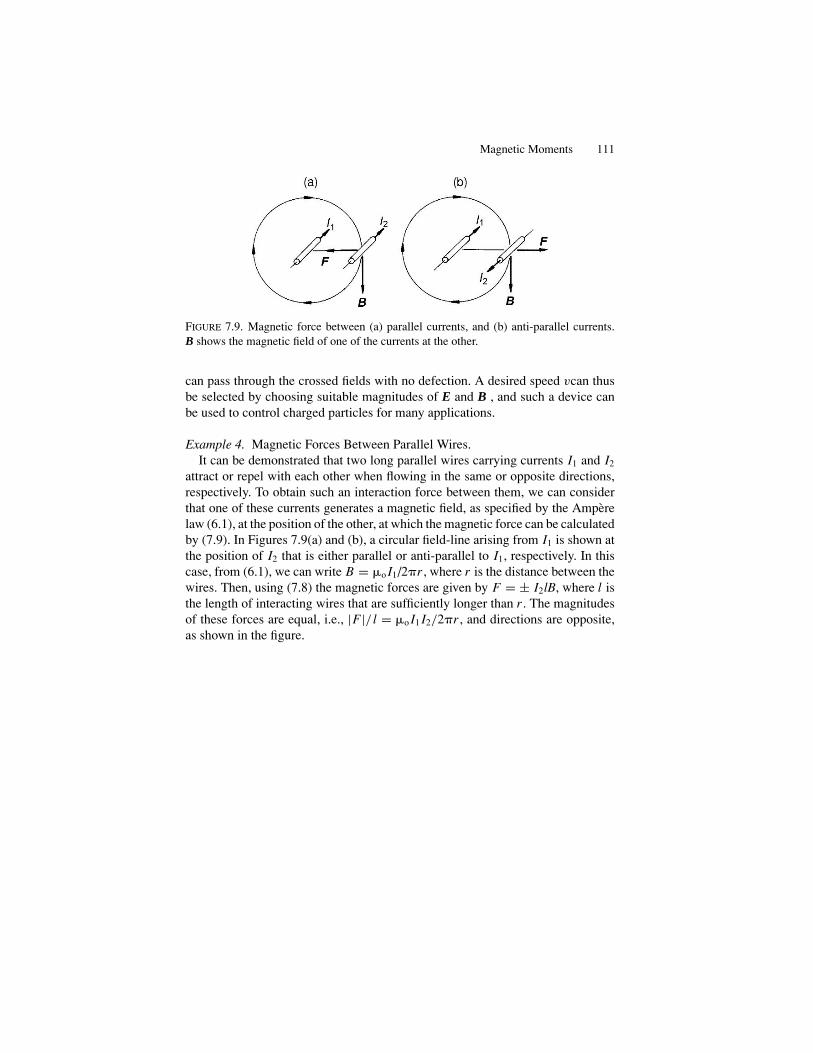
Magnetic Moments 111
FIGURE 7.9. Magnetic force between (a) parallel currents, and (b) anti-parallel currents.B shows the magnetic field of one of the currents at the other.
can pass through the crossed fields with no defection. A desired speed vcan thusbe selected by choosing suitable magnitudes of E and B , and such a device canbe used to control charged particles for many applications.
Example 4. Magnetic Forces Between Parallel Wires.It can be demonstrated that two long parallel wires carrying currents I1 and I2
attract or repel with each other when flowing in the same or opposite directions,respectively. To obtain such an interaction force between them, we can considerthat one of these currents generates a magnetic field, as specified by the Amperelaw (6.1), at the position of the other, at which the magnetic force can be calculatedby (7.9). In Figures 7.9(a) and (b), a circular field-line arising from I1 is shown atthe position of I2 that is either parallel or anti-parallel to I1, respectively. In thiscase, from (6.1), we can write B = �o I1/2�r , where r is the distance between thewires. Then, using (7.8) the magnetic forces are given by F = ± I2lB, where l isthe length of interacting wires that are sufficiently longer than r . The magnitudesof these forces are equal, i.e., |F |/ l = �o I1 I2/2�r , and directions are opposite,as shown in the figure.

8Scalar and Vector Potentials
8.1. Magnets
Natural magnets played the central role in magnetic studies in early days, leading tothe Ampere law of a magnetic field, which was discovered by using iron magnets.Characterized as N- and S-poles, magnetic charges were postulated by analogy toelectric charges. However, it was only after Heisenberg’s quantum theory (1928)that the origin of magnetism was attributed to correlated electronic spin angularmomenta in materials.
With iron magnets and by induction experiments, it was recognized a currentcarrying coil generates such magnetic poles upon which field-lines converge, justlike in natural magnets. Figure 8.1 illustrates a bar magnet and a uniform coilcarrying an electric current, where voltages V (t) induced by moving a searchcoil Lo along their axes are plotted as a function of time t . Positive and negativevoltage pulses can be observed near the end regions as shown, indicating high fluxdensities of magnetic field-lines corresponding to the magnetic poles. In the middlepart of the coil no appreciable induction takes place because of nearly uniform fluxdensities. On the other hand, to interpret the observed results from the magnet, wehave to consider the internal magnetic flux M, which is virtually constant due tosaturated spontaneous magnetization. Related to these poles, magnetic fields existinside and outside of the magnetic material, where the flux of field-lines should bedescribed by the respective densities; that is,
Bin = �o Hin + M and Bout = �o Hout. (8.1)
A significant feature of the magnetism is that a single magnetic pole cannotbe isolated in nature. If such a single pole could exist at all, it was believed thatmagnetic field-lines would emerge from it, similar to what is seen with electriccharges. However magnetic poles appear always in pairs, and no attempt to separatethem has been successful. Therefore, accepting this phenomenon as a fact in nature,we consider it a law of magnetism. In fact, ionic and molecular magnetic momentsare responsible for such a pair of poles, so that macroscopically the absence ofsingle magnetic charges can be expressed by zero density per volume, i.e., �m = 0.Noting that the Gauss theorem expresses the general relation between flux densities
112
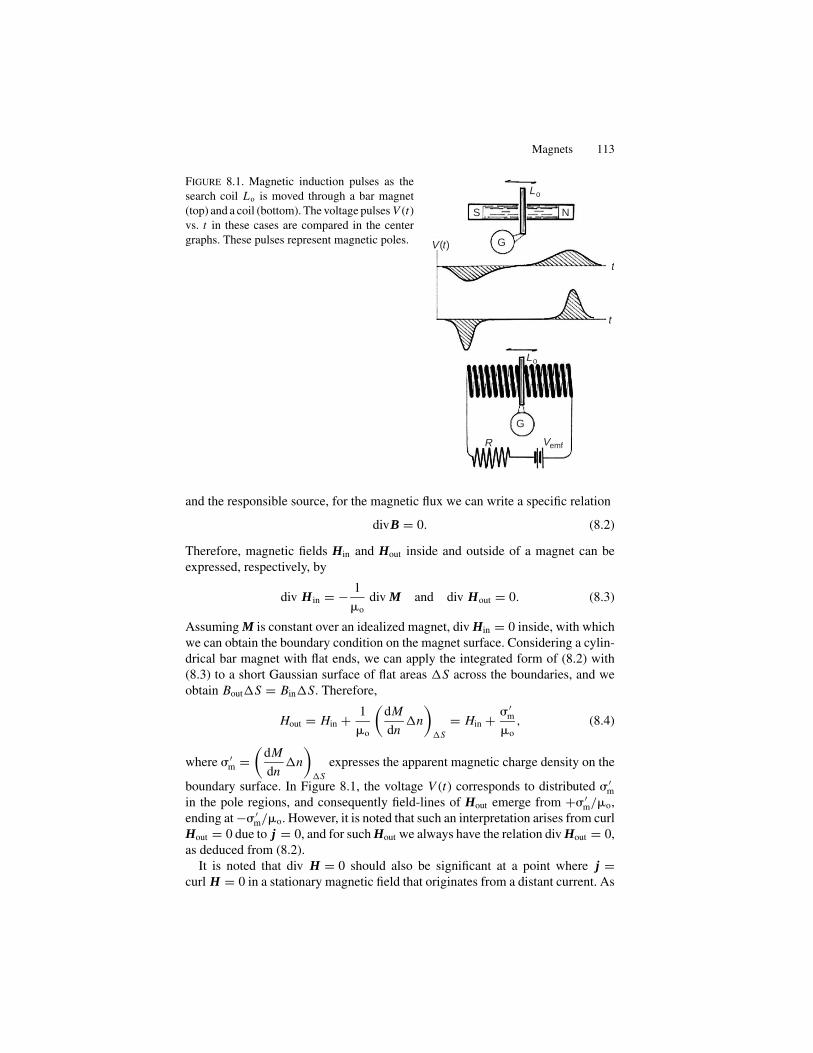
Magnets 113
Lo
Lo
R Vemf
V(t)
S N
G
G
t
t
FIGURE 8.1. Magnetic induction pulses as the
search coil Lo is moved through a bar magnet
(top) and a coil (bottom). The voltage pulses V (t)vs. t in these cases are compared in the center
graphs. These pulses represent magnetic poles.
and the responsible source, for the magnetic flux we can write a specific relation
divB = 0. (8.2)
Therefore, magnetic fields Hin and Hout inside and outside of a magnet can beexpressed, respectively, by
div Hin = − 1
�o
div M and div Hout = 0. (8.3)
Assuming M is constant over an idealized magnet, div Hin = 0 inside, with whichwe can obtain the boundary condition on the magnet surface. Considering a cylin-drical bar magnet with flat ends, we can apply the integrated form of (8.2) with(8.3) to a short Gaussian surface of flat areas �S across the boundaries, and weobtain Bout�S = Bin�S. Therefore,
Hout = Hin + 1
�o
(dM
dn�n
)�S
= Hin + �′m
�o
, (8.4)
where �′m =
(dM
dn�n
)�S
expresses the apparent magnetic charge density on the
boundary surface. In Figure 8.1, the voltage V (t) corresponds to distributed �′m
in the pole regions, and consequently field-lines of Hout emerge from +�′m/�o,
ending at −�′m/�o. However, it is noted that such an interpretation arises from curl
Hout = 0 due to j = 0, and for such Hout we always have the relation div Hout = 0,as deduced from (8.2).
It is noted that div H = 0 should also be significant at a point where j =curl H = 0 in a stationary magnetic field that originates from a distant current. As

114 8. Scalar and Vector Potentials
FIGURE 8.2. A chain of differential coils
of lengths �s1, �s2, �s3, . . . , moni-
toring magnitudes of magnetic fields
H1, H2, H3, . . . . (R.W. Pohl, Elec-trizitatslehre)
discussed in Section 6.6, to obtain the solution at such a point, it is not sufficientto solve curl H = 0, but necessary for H to satisfy div H = 0. In any case, theequation div B = 0 holds in both magnetic and a steady current fields, and (8.2)is regarded as a fundamental equation for any magnetic field.
8.2. Pohl’s Magnetic Potentiometer
Using a search coil, it is possible to map a magnetic field in terms of the inducedvoltage pulse U . As implied by the relation B = �o H in empty space, a smallsolenoid can be used for investigating the vector character of a distributed field. Fora long flexible solenoid of a cross-sectional area S = Sn, we consider a short partof length ds = dsn, whose orientation is represented by n. A magnetic inductionshould occur as related to the rate d(B.S)/dt , which is proportional to H.ds,and both are specified by n. In such a device, plus and minus voltage pulses inpair can be recorded in Lo, as illustrated in Figure 8.1. Pohl constructed a longflexible solenoid attached to a galvanometer, which was, in fact, displayed fordemonstration in his lecture theater at Gottigen. Figures (8.2) and (8.3) showsketches of his device and related concept, which is quoted in the following fromhis textbook “Elektrizitatslehre.”
With such a device the experimental purpose is two-fold: to identify locations for
high and low flux densities in the field, and to verify that∫ B
AH.ds is independent
of the path of integration terminated at points A and B. Figure 8.2 illustrates thatsuch a long solenoid can be considered to consist of small segments of lengths dsi ,
so that the integral∫ B
AH.ds can be replaced approximately by the sum
∑i Hi.ds i
where voltage pulses at each joint of adjacent segments are cancelled. Figure 8.3illustrates some practical operations of Pohl’s device. Here, Figure 8.3(a) showsmeasurements of voltage pulses at the ends a and b of a solenoidal magnet, andin Figure 8.3(b) is shown an instrument that measures the N and S poles of ahorseshoe magnet. In these experiments it is significant that all the results areindependent of the device’s “shape,” confirming that the integral is determinedonly by the end positions. Figures 8.3(c) and 8.3(d) illustrate experiments for such
voltage pulses at the ends of a solenoidal coil, giving the same results∫ b
a H.ds =nI, where I is current and n is number of turns per length, confirming the Amperelaw.

Pohl’s Magnetic Potentiometer 115
FIGURE 8.3. Demonstrations of Pohl’s magnetic potentiometers. (a) Obtaining magnetic
induction pulses from a coil, and (b) from a horseshoe magnet. (c) and (d) are for measure-
ments with a long air-core solenoid. (R.W. Pohl, Electrizitatslehre)
As signified by the Ampere law, the field of H(r) is not conservative, howeverin the outside space of a magnet, H.ds can be expressed by a perfect differentialof a scalar function Vm(r ), i.e., −H.ds = dVm between the limits. Such a scalarfunction Vm(r), called pseudo-potential, is useful for calculation of magnetostaticproblems. If a magnetic field signified by a pair of apparent charges, the pseudo-potential is particularly useful. Writing that
Hout = −grad Vm (8.5)
and the relation
div Hin = −�′m
�o
for connecting Hin and Hout at the boundaries, we have to satisfy the Laplace–Poisson equation for Vm , i.e.,
∇2Vm = 0 and ∇2Vm = −�′m
�o
. (8.6)
Magnetostatic problems can be solved with such a pseudo-potential Vm analogousto electrostatic cases, for which Pohl’s potentiometer is designed to determine the
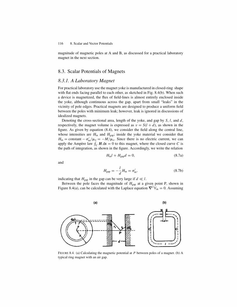
116 8. Scalar and Vector Potentials
magnitude of magnetic poles at A and B, as discussed for a practical laboratorymagnet in the next section.
8.3. Scalar Potentials of Magnets
8.3.1. A Laboratory Magnet
For practical laboratory use the magnet yoke is manufactured in closed-ring shapewith flat ends facing parallel to each other, as sketched in Fig. 8.4(b). When sucha device is magnetized, the flux of field-lines is almost entirely enclosed insidethe yoke, although continuous across the gap, apart from small “leaks” in thevicinity of pole edges. Practical magnets are designed to produce a uniform fieldbetween the poles with minimum leak; however, leak is ignored in discussions ofidealized magnets.
Denoting the cross-sectional area, length of the yoke, and gap by S, l, and d,respectively, the magnet volume is expressed as v = S(l + d), as shown in thefigure. As given by equation (8.4), we consider the field along the central line,whose intensities are Hin and Hgap; inside the yoke material we consider thatHin = constant − �′
m/�o = −M/�o. Since there is no electric current, we canapply the Ampere law
∮C H.ds = 0 to this magnet, where the closed curve C is
the path of integration, as shown in the figure. Accordingly, we write the relation
Hinl + Hgapd = 0, (8.7a)
and
Hgap = − l
dHin = �′
m, (8.7b)
indicating that Hgap in the gap can be very large if d � l.Between the pole faces the magnitude of Hgap at a given point P, shown in
Figure 8.4(a), can be calculated with the Laplace equation ∇2Vm = 0. Assuming
FIGURE 8.4. (a) Calculating the magnetic potential at P between poles of a magnet. (b) A
typical ring magnet with an air gap.

Scalar Potentials of Magnets 117
circular pole-faces, we set cylindrical coordinates � , �, z with respect to the centerO in the gap and express magnetic potentials due to charge elements �′
m(r1)dS1
and �′m(r2)dS2 on the N- and S-surfaces, respectively, where their positions are
specified by vectors r1 and r2 from O. At the point P, where r = (0, 0, z), thepotential is generally expressed by
Vm(r ) = 1
4��o
∫S
�′m
(r ′) dS∣∣r − r ′∣∣ .
Assuming that �′m is constant over a circular region 0 ≤ � ≤ a′ on the pole faces,
this potential is written for the present case as
Vm(z) = 1
4��o
(∫S1
dS1
r1
−∫
S2
dS2
r2
),
where
∫S1
dS1
r1
=∫ 2�
0
d�
∫ a′
0
�d�√� 2 + z2
= 2�(√
a′2 + z2 − z)
≈ 2�(a′ − z
)
and ∫S2
dS2
r2
= 2�{a′ − (d − z)
}.
Hence, we obtain
Vm(z) = �′m
2�o
(d − 2z) and Hgap = −∂Vm (z)
∂z= �′
m
�o
.
In the above argument, in the field across the narrow gap, the lines of Hgap startfrom �′
m and end at −�′m. The magnitude of �′
m determined by the magnetization Mis a function of temperature, but is usually adjustable in adjustable electromagnets.In any case, a certain amount of energy u is required for keeping �′
m on the polesurfaces, which can be calculated as the amount to increase charges from 0 to ±�′
m,i.e.,
u =∫ �′
m
0
Hgapd�′m = 1
�o
∫ �′m
0
�′md�′
m = �′m
2
2�o
per unit area.Therefore, we can consider that a magnetic energy Um = uSd is stored in the
gap space, which is responsible for a strong attractive force Fm between the poles.That is,
Fm = −∂Um
∂d= −uS .

118 8. Scalar and Vector Potentials
Exercise. A small current-carrying coil (cross-sectional area S, turn number N,length l) is suspended in perpendicular to a uniform horizontal magnetic fieldB = �o H . Express the magnetic moment, angular momentum of this coil anddiscuss the concept of magnetic charges as related to its rotational behavior.
8.3.2. A Uniformly Magnetized Sphere
A ferromagnet is spontaneously magnetized under ambient conditions, where themagnetization appears often along a unique axis of the crystalline state. An ironblock can be fabricated in spherical shape showing axial magnetization related toapparent magnetic charges in high densities on opposite surfaces. Such a magne-tized sphere is characterized by internal flux of field-lines M in near parallel withthe axis. On the other hand, the vector M of the sphere appears to be a dipolarmoment, when observed at a distant point.
For such a spherical magnet we have a basic relation curl H = 0 in the outsidespace, where the field H can be expressed by a scalar potential Vm, i.e., H =−grad Vm. On the other hand, from the basic law div B = 0 we can write div H =− 1
�o
div M , and hence the potential Vm should be determined by the Poisson
equation ∇2Vm = 1
�o
div M. Applying this idea to outside of the sphere, because
M = 0 we are to solve the Laplace equation ∇2Vm = 0, whereas inside the spherewe also have the Laplace equation because M = constant. Solutions of the Laplaceequation can therefore be connected on the spherical surface, as required by theboundary conditions
(Hout − Hin)tangent = 0 and (Hout − Hin)normal = �′m. (8.8)
Here, the constant magnetization M is responsible for Hin, as given by Hin =−M/�o, whereas Hout should be represented approximately by a dipolar field ata distant point.
In this problem, the potential function in axial symmetry can be obtained from theLaplace equation ∇2Vm = 0, which can be solved by analogy with an equivalentelectrostatic problem. As discussed for the electrostatic case, the magnetic potentialin axial symmetry can be expressed as
Vm(r, �) =∑
n
(Anrn + Bn
rn +1
)Pn (cos �),
where the constants An and Bn should be determined by boundary conditions onthe sphere.
Inside the sphere r < R, the potential should be given exclusively by terms ofAn, because terms of Bn are singular at r = 0. On the other hand, for r > R thefield is dominated by Bn terms, because An terms become infinite for r → ∞.Further, only the term for n = 1 is necessary for the spherical problem because
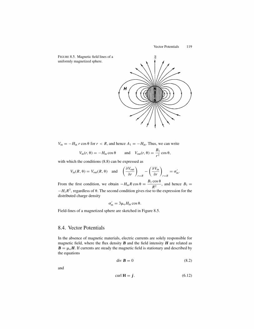
Vector Potentials 119
FIGURE 8.5. Magnetic field lines of a
uniformly magnetized sphere.
Vm = −Hin r cos � for r < R, and hence A1 = −Hin. Thus, we can write
Vin(r, �) = −Hin cos � and Vout(r, �) = B1
r2cos �,
with which the conditions (8.8) can be expressed as
Vin(R, �) = Vout(R, �) and
(∂Vout
∂r
)r=R
−(
∂Vin
∂r
)r=R
= �′m.
From the first condition, we obtain −Hin R cos � = B1 cos �
R2, and hence B1 =
−H1 R3, regardless of �. The second condition gives rise to the expression for thedistributed charge density
�′m = 3�o Hin cos �.
Field-lines of a magnetized sphere are sketched in Figure 8.5.
8.4. Vector Potentials
In the absence of magnetic materials, electric currents are solely responsible formagnetic field, where the flux density B and the field intensity H are related asB = �o H. If currents are steady the magnetic field is stationary and described bythe equations
div B = 0 (8.2)
and
curl H = j . (6.12)
120 8. Scalar and Vector Potentials
Such a magnetic field is not conservative in character, and hence cannot be de-scribed by a scalar potential. In this case, it is noted that (8.2) can be satisfied bya vector A in a manner that
B = curl A (8.9)
because of the identity div(curl A) ≡ 0, where the vector A is called a vectorpotential. In this definition there is an ambiguity because another vector A′ definedas A′ = A + grad � , where � is a scalar function, can also satisfy the equationdiv B = 0, and hence curl A′ = curl A. Accordingly, using this ambiguity, we candefine the vector potential A with additional conditions
divA = 0 and ∇2� = 0. (8.10)
With (8.10) and the identity relation
curl(curlA) = grad(divA) − ∇2 A = −∇2 A,
the Ampere law, curl H = j can be written in the form of Poisson’s equation, i.e.,
−∇2 A = �o j, (8.11)
indicating that the vector potential A at a given point r can be determined by acurrent density j. However, if j = 0 at this point r, (8.11) is the Laplace equation
∇2 A = 0. (8.12)
Similar to electrostatic cases, we need to obtain the vector potential A(r) ata given point r when a current distribution j(r ′) is specified at another pointr ′. The potential A(r) is determined by the Laplace equation, ∇2 A (r ) = 0, ifj(r ) = 0, whereas the current density j(r ′) at r ′ is related with A(r ′) by thePoisson equation ∇2 A
(r ′) = −�o j
(r ′). Therefore, we are to look for A(r) as
related to A(r ′), and the problem can be analyzed by the Greens function method.Here, we simply transfer the result to the present problem for stationary currents,as already discussed the detail in Chapter 4.
For a given current density j(r ′) at r ′, the vector potential A(r) at r can beexpressed by
A (r ) = �o
4�
∫v(r ′)
j(r ′)∣∣r − r ′∣∣d3r ′, (8.13)
where the integral is performed over the volume v(r ′) of distributed currents. Theflux density at r can then be calculated by B(r ) = curlr A(r ). To calculate A(r ),we replace curlr of the integrand in (8.13) by
curlrj(r ′)∣∣r − r ′∣∣ = − j
(r ′) × (
r − r ′)∣∣r − r ′∣∣3
,
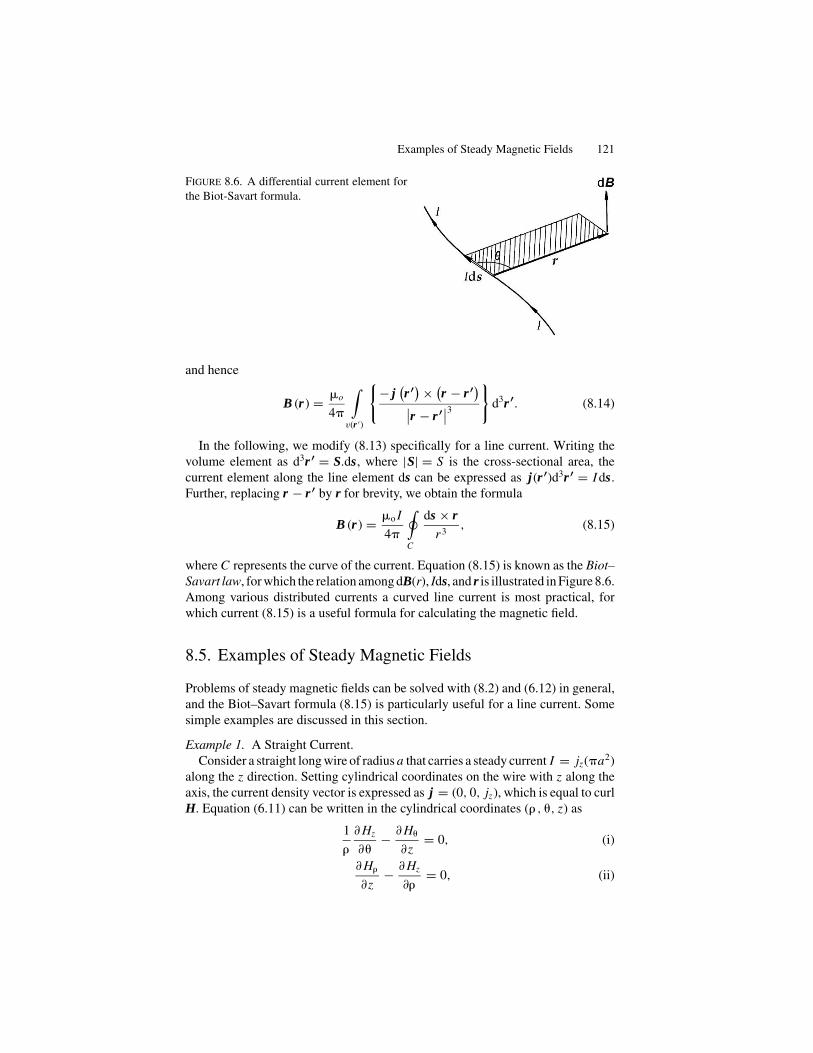
Examples of Steady Magnetic Fields 121
FIGURE 8.6. A differential current element for
the Biot-Savart formula.
and hence
B (r ) = �o
4�
∫v(r ′)
{− j
(r ′) × (
r − r ′)∣∣r − r ′∣∣3
}d3r ′. (8.14)
In the following, we modify (8.13) specifically for a line current. Writing thevolume element as d3r ′ = S.ds, where |S| = S is the cross-sectional area, thecurrent element along the line element ds can be expressed as j(r ′)d3r ′ = I ds.Further, replacing r − r ′ by r for brevity, we obtain the formula
B (r ) = �o I
4�
∮C
ds × rr3
, (8.15)
where C represents the curve of the current. Equation (8.15) is known as the Biot–Savart law, for which the relation among dB(r), Ids, and r is illustrated in Figure 8.6.Among various distributed currents a curved line current is most practical, forwhich current (8.15) is a useful formula for calculating the magnetic field.
8.5. Examples of Steady Magnetic Fields
Problems of steady magnetic fields can be solved with (8.2) and (6.12) in general,and the Biot–Savart formula (8.15) is particularly useful for a line current. Somesimple examples are discussed in this section.
Example 1. A Straight Current.Consider a straight long wire of radius a that carries a steady current I = jz(�a2)
along the z direction. Setting cylindrical coordinates on the wire with z along theaxis, the current density vector is expressed as j = (0, 0, jz), which is equal to curlH. Equation (6.11) can be written in the cylindrical coordinates (� , �, z) as
1
�
∂ Hz
∂�− ∂ H�
∂z= 0, (i)
∂ H�
∂z− ∂ Hz
∂�= 0, (ii)

122 8. Scalar and Vector Potentials
and
1
�
∂(� H�)
∂�− 1
�
∂ H�
∂�= jz . (iii)
The equation div H = 0 can also be expressed as
1
�
∂(� H� )
∂�+ 1
�
∂ H�
∂�+ ∂ Hz
∂z= 0. (iv)
By symmetry, Hz and H� should be constant, and hence (i) is not necessary. From(ii), Hz is constant and independent of � with no relation to jz , and thereforeinsignificant. Then from (iv), we have
∂(� H� )
∂�= 0, hence H� = c
�
where the constant c should be zero in order for H� to be finite at � = 0, and henceH� = 0. Thus, only H� is significant, for which (iii) should be solved against agiven jz . Namely,
1
�
d(� H�)
d�= jz, (v)
from which we obtain jz = I/�a2 for 0 < � < a, whereas jz = 0 for � > a.Integrating (v), we obtain the solutions
H� = 1
2jz� + c′
�and H� = c′′
�,
in these regions, respectively. Here, the constant c′ should be zero in order for H� tobe definite at � = 0. Further, on the surface of the wire � = a, these two H� insideand outside should be connected continuously because j has only a z component,and therefore c′′ = I/2�. Thus, we obtain the expressions (H�)in = 1
2jz� and
(H�)out = I/2�� , describing circular field-lines in these regions.
Example 2. A Uniform Solenoid.We discussed a long solenoid in Section 6.3, where the magnetic field inside
was considered uniform, although unverified from the first principle. Here, wediscuss the problem with the basic equation (6.11) for a steady current j. Settingthe z direction on the solenoid axis, we use cylindrical coordinates, � , � and z.Assume that the coiled wire occupies a narrow radial region between � = a and� = b, in which a and b are considered to be almost equal, but a < b, and that thenumber of turns per length of the coil is n. Then, the steady current is expressed by−I = j�(b − a)/n, where j� can be assumed to be constant, and a ≈ b. In sucha long solenoid, the field vector H should only be a function of � , independentof � and z, hence, using equations (i) to (iv) in Example 8.1, we can derive thefollowing equations for the components H� , H� and Hz . That is,
1
�
d(� H� )
d�= 0,
1
�
d(� H� )
d�= 0, and − dHz
d�= j�.

Examples of Steady Magnetic Fields 123
FIGURE 8.7. (a) An application of the Biot-Savart formula to a ring current I . (b) Calculating
the magnetic field H at an off-axis point P due to a ring current I .
Integrating the first and second relations, we obtain that H� = c/� and H� = c′/� ,where the constants c and c′ should both be zero in order to avoid singularities at� = 0. Hence H� = H� = 0. From the third equation in the above, we can easilyobtain that
Hz = −∫ b
aj�d� = − j�(b − a) = nI,
describing a uniform field for a constant I .
Example 3. Magnetic Field on the Axis of a Ring Current.A stationary current on a conducting ring is hypothetical, unless the current
source, e.g., a battery, is specified on the ring. However, the problem is discussed,serving as a model for calculating the field in a coil or of an orbiting electron. Wecan apply the Biot–Savart formula (8.15) to calculate the magnetic field at a point Pon the axis perpendicular to the plane of the ring current, as shown in Figure 8.7(a).
Consider two current elements I ds1 and I ds2 that are located on the ringsymmetrically with respect to the ring center. Related differential fields dB1 anddB2 at P are perpendicular to the planes of ds1 × r1 and ds2 × r2, where r1 and r2
are the distances between these elements and P, respectively. These vector fieldscan be added as shown in the figure, i.e.,
dB = dB1 + dB2 = �o I
4�
(ds1 × r1
r31
+ ds2 × r2
r32
),
which is parallel to the z-axis at P where |r1| = |r2| = r . Therefore,
B =∮
|dB| cos � = �o I
4�cos �
∮sin �ds
r2
= �o I cos �
4�r2
(2 ×
∫ �r
0
ds
)= �o I cos �
2r, (8.16)
124 8. Scalar and Vector Potentials
where � = 12�. If P is at the center of the ring, � = 0 and r = a (the radius), and
hence B = �o I/2a.
Example 4. Off-Axis Fields of a Ring Current.In this example, we calculate the magnetic field at an off-axis point P of a ring
current, as shown in Fig. 8.7(b).The vector potential at the point P(r ), where r = (r, �, ), is given by
A (r ) = �o
4�
∮ds ′∣∣r − r ′∣∣ ,
where r ′ = (a, �, 12�) and
ds′ = (−a sin � d�, a cos � d�, 0),
(r − r ′)2 = (r sin � cos − a cos �)2 + (r sin � sin − a sin �)2 + (r cos )2
= r2 + a2 − 2ra sin � cos( − �).
Since the differential ring current I ds is on the xy-plane, the vector potential issignified only by A component, which is expressed as
A = −Ax sin + Ay sin = �o I a
4�
∫ 2�
0
cos ( − �) d�√r2 + a2 − 2ra sin � cos ( − �)
Writing − � = and 2 ar sin �/(r2 + a2) = �, this expression can be simpli-fied as
A = �oIa
4�√
r2 + a2
∫ 2�
0
cos √1 − � cos
d .
It is noted that for all points of (r , �, ), the parameter � is in the range 0 ≤ � ≤ 1,except for � = 1
2�. Therefore, we can expand the above integrand into a Taylor
series with respect to a small �; that is,
1√1 − � cos
= 1 + 1
2� cos + 3
8�2 cos3 + · · · .
Using the formula
∫ 2�
0
cos2n d = 2� (2n!)
22n (n!)2and
∫ 2�
0
cos2n+1 d = 0,
we obtain
A = �o I a2
4
r sin �(r2 + a2
)3/2
(1 + 15
8
a2r2
(r2 + a2
)2sin2 � + · · ·
).
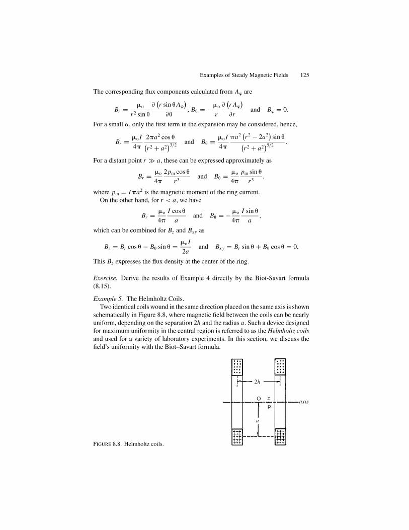
Examples of Steady Magnetic Fields 125
The corresponding flux components calculated from A are
Br = �o
r2 sin �
∂(r sin � A
)∂�
, B� = −�o
r
∂(r A
)∂r
and B = 0.
For a small �, only the first term in the expansion may be considered, hence,
Br = �o I
4�
2�a2 cos �(r2 + a2
)3/2and B� = �o I
4�
�a2(r2 − 2a2
)sin �(
r2 + a2)5/2
.
For a distant point r a, these can be expressed approximately as
Br = �o
4�
2pm cos �
r3and B� = �o
4�
pm sin �
r3,
where pm = I �a2 is the magnetic moment of the ring current.On the other hand, for r < a, we have
Br = �o
4�
I cos �
aand B� = − �o
4�
I sin �
a,
which can be combined for Bz and Bxy as
Bz = Br cos � − B� sin � = �o I
2aand Bxy = Br sin � + B� cos � = 0.
This Bz expresses the flux density at the center of the ring.
Exercise. Derive the results of Example 4 directly by the Biot-Savart formula(8.15).
Example 5. The Helmholtz Coils.Two identical coils wound in the same direction placed on the same axis is shown
schematically in Figure 8.8, where magnetic field between the coils can be nearlyuniform, depending on the separation 2h and the radius a. Such a device designedfor maximum uniformity in the central region is referred to as the Helmholtz coilsand used for a variety of laboratory experiments. In this section, we discuss thefield’s uniformity with the Biot–Savart formula.
2h
zaxis
a
O
P
FIGURE 8.8. Helmholtz coils.

126 8. Scalar and Vector Potentials
We consider a point P2 at a distance z from the center O on the axis. In themagnetic field of a coil of N turns, the flux density can be described by the formula(8.15) modified for the present problem. The point P can be specified by thedistances h + z and h − z from the centers of coils, therefore the total flux densityat P is expressed by
Bz = N�o I
2
⎡⎢⎢⎢⎣
1{1 + (h − a)2
a2
}3/2+ 1{
1 + (h + a)2
a2
}3/2
⎤⎥⎥⎥⎦ .
Writing h/a = m, z/a = � , and further defining p = m/(1 + m2) andq = 1/(1 + m2), this expression can be changed to
Bz = �o I q3/2
2a
{1(
1 − 2p� + q� 2)3/2
+ 1(1 + 2p� + q� 2
)3/2
}.
Considering z < a for the Helmholtz coils, this equation can be expanded intoa power series of a small parameter � , where all terms of odd power vanish bysymmetry. Therefore, we keep terms proportional to � 2 and � 4, ignoring higherterms as insignificant. After some calculation, we obtain
Bz = �o I q3/2
a
{1 +
(−3q
2+ 15p2
2
)� 2 +
(15q2
8− 105p2q
4+ 315p4
)� 4
}.
If the coefficient of � 2 is taken as zero, the density Bz is homogeneous in thevicinity of � = 0, i.e., z = 0, at least approximately, for which we have the relationq = 5p2, or m = 1. Hence, the uniform field is approximately obtained at the centerO if 2h = a. In this case, the uniformity is given by the coefficient of � 4 in the lastexpression, which is calculated as –144/125. The Helmholtz field is then given by
Bz = �o I
a
(4
5
)3/2 (1 − 144z4
125a4
).
8.6. Vector and Scalar Potentials of a Magnetic Moment
In Section 7.3 a magnetic moment was defined for a rectangular wire of area S,carrying a current I , to rotate in a uniform magnetic field, which was expressed aspm = I S in (7.9). In general, such a magnetic moment can be defined for stationarycurrent distribution j (r′) from its vector potential A (r). We can expand A (r) givenby (8.13) into power series of r ′/r , assuming r > r ′. Namely,
1∣∣r − r ′∣∣ = 1
r− r ′ · ∇
(1
r
)+ 1
2!
∑ij
x ′i x
′j
∂2
∂xi∂xj
(1
r
)+ . . . ,

Vector and Scalar Potentials of a Magnetic Moment 127
and
A(r ) = Ao(r ) + A1(r ) + A2(r ) + . . . ,
where
Ao(r ) = �o
4�r
∫v(r ′)
j(r ′) d3r ′,
A1 (r ) = − �o
4�
∫v(r ′)
j(r ′) {
r ′ × ∇(
1
r
)}d3r ′,
A2 (r ) = �o
8�
∑ {∫v(r ′)
j(r ′) x ′
i x′j d
3r ′}
∂2
∂xi∂xj
(1
r
),
...
First, we can prove that Ao(r) = 0 for a circular closed current. For a ring current,we have d3(r) = S.ds′ and j(r′).S = I , where S is the cross-sectional area of thecurrent path C . We can therefore write∫
v(r ′)j(r ′)d3r ′ = S
∮C
j(r ′)ds′ = I∮
Cds′ = 0,
and Ao (r ) = 0.For the second term, A1(r), the integrand can be manipulated as
j(r ′) (
r ′.∇1
r
)= 1
2
[j(r ′) (
r ′.∇1
r
)− r ′
{j(r ′) .∇1
r
}]
+ 1
2
[j(r ′) (
r ′.∇1
r
)+ r ′
{j(r ′) .∇1
r
}].
For a circular line current along C , j(r′)d3 r ′ = I ds, so that the second square-bracketed term times d3r′ can be written as proportional to
ds′(
r ′.∇1
r
)+ r ′
(ds′.∇1
r
)= d
{r ′
(s′.∇1
r
)},
which is a perfect differential, giving rise to zero when integrated along C . There-fore, contributed by the first term in [ ], we have
A1(r ) = − �o
4�
{ ∫v(r ′)
r ′ × j(r ′)
2d3r ′
}× ∇1
r,
from which we can define the magnetic moment as
pm = 1
2
∫v(r ′)
r ′ × j(r ′) d3r ′. (8.17)
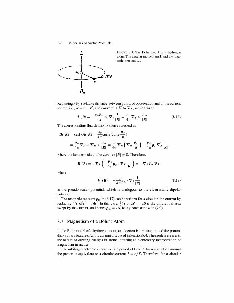
128 8. Scalar and Vector Potentials
FIGURE 8.9. The Bohr model of a hydrogen
atom. The angular momentum L and the mag-
netic moment pm.
Replacing r by a relative distance between points of observation and of the currentsource, i.e., R = r − r ′, and converting ∇ to ∇R , we can write
A1(R) = −�o pm
4�× ∇R
1
|R| = �o
4�∇R × pm
|R| . (8.18)
The corresponding flux density is then expressed as
B1(R) = curlR A1(R) = �o
4�curlR(curlR
pm
|R| )
= �o
4�∇R × ∇R × pm
|R| = �o
4�∇R
(∇R .
pm
|R|)
− �o
4�pm∇2
R
1
|R| ,
where the last term should be zero for |R| �= 0. Therefore,
B1(R) = −∇R
(− �o
4�pm · ∇R
1
|R|)
= −∇R Vm (R) ,
where
Vm(R) = − �o
4�pm · ∇R
1
|R| (8.19)
is the pseudo-scalar potential, which is analogous to the electrostatic dipolarpotential.
The magnetic moment pm in (8.17) can be written for a circular line current byreplacing j (r′)d3r′ = I ds′. In this case, 1
2( r′× ds′) = dS is the differential area
swept by the current, and hence pm = I S, being consistent with (7.9).
8.7. Magnetism of a Bohr’s Atom
In the Bohr model of a hydrogen atom, an electron is orbiting around the proton,displaying a feature of a ring current discussed in Section 8.4. The model representsthe nature of orbiting charges in atoms, offering an elementary interpretation ofmagnetism in matter.
The orbiting electronic charge –e in a period of time T for a revolution aroundthe proton is equivalent to a circular current I = e/T . Therefore, for a circular
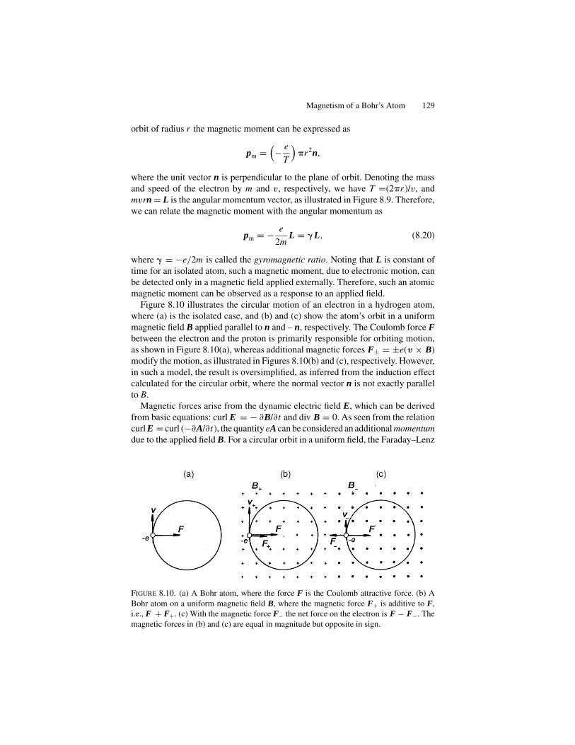
Magnetism of a Bohr’s Atom 129
orbit of radius r the magnetic moment can be expressed as
pm =(− e
T
)�r2n,
where the unit vector n is perpendicular to the plane of orbit. Denoting the massand speed of the electron by m and v, respectively, we have T =(2�r )/v, andmvrn = L is the angular momentum vector, as illustrated in Figure 8.9. Therefore,we can relate the magnetic moment with the angular momentum as
pm = − e
2mL = L, (8.20)
where = −e/2m is called the gyromagnetic ratio. Noting that L is constant oftime for an isolated atom, such a magnetic moment, due to electronic motion, canbe detected only in a magnetic field applied externally. Therefore, such an atomicmagnetic moment can be observed as a response to an applied field.
Figure 8.10 illustrates the circular motion of an electron in a hydrogen atom,where (a) is the isolated case, and (b) and (c) show the atom’s orbit in a uniformmagnetic field B applied parallel to n and – n, respectively. The Coulomb force Fbetween the electron and the proton is primarily responsible for orbiting motion,as shown in Figure 8.10(a), whereas additional magnetic forces F± = ±e(v × B)modify the motion, as illustrated in Figures 8.10(b) and (c), respectively. However,in such a model, the result is oversimplified, as inferred from the induction effectcalculated for the circular orbit, where the normal vector n is not exactly parallelto B.
Magnetic forces arise from the dynamic electric field E, which can be derivedfrom basic equations: curl E = − ∂B/∂t and div B = 0. As seen from the relationcurl E = curl (−∂A/∂t), the quantity eA can be considered an additional momentumdue to the applied field B. For a circular orbit in a uniform field, the Faraday–Lenz
FIGURE 8.10. (a) A Bohr atom, where the force F is the Coulomb attractive force. (b) A
Bohr atom on a uniform magnetic field B, where the magnetic force F+ is additive to F,
i.e., F + F+. (c) With the magnetic force F− the net force on the electron is F − F−. The
magnetic forces in (b) and (c) are equal in magnitude but opposite in sign.

130 8. Scalar and Vector Potentials
law can be expressed as
− d
dtB ·
(∮C
r × ds2
)=
∮C
E · ds = −∮C
∂ A∂t
· ds,
from which we can derive an expression for the vector potential A of a uniform B,that is,
A = 1
2(B × r ) . (8.21)
In a uniform field B, the Hamiltonian of the orbiting electron can be written as
H = 1
2m(p + eA)2 − e2
4�εor
= Ho + e
mp.A + e2
2mA2, (8.22)
where Ho = p2
2m− e2
4�εoris the Hamiltonian when B = 0, and A is given by
(8.22). The second term in (8.22) can be modified as
e
mp.A = e
2m{p. (B × r )} = e
2m{(r × p) .B} = −pm · B, (8.23)
representing the magnetic dipolar energy Um = −pm · B in a magnetic field, mak-ing the dipolar direction stable if pm||B, similar to the electric dipolar energy(4.26a). For a system of N atoms, the corresponding macroscopic energy W1
should be related to the time average of pm over many revolutions, and expressedby W1 = −N〈pm〉.B.
The third term in (8.22) can be expressed for B = (0, 0, B) as
e2
2mA2 = e2
8m
(x2 + y2
)B2,
which should also be averaged over many revolutions of the orbiting electron torepresent a macroscopic energy. Therefore, we consider that 〈x2 + y2〉 = 1
2〈r2〉,
where r2 = x2 + y2 + z2, resulting in a macroscopic energy W2
W2 = Ne2〈r2〉B2
12m.
On applying an external field B, a system of N atoms gains a macroscopicenergy W = W1 + W2, for which we can define the magnetic susceptibility by� = −∂W /∂ B. Hence, we have
� = �1 + �2 where �1 = N < pm 0 and �2 = −Ne2〈r2〉6m
B < 0.
In this context, for such a system of independent atoms, the magnetic susceptibilitycan be positive or negative, corresponding to paramagnetic or diamagnetic cases,respectively.

Magnetism of a Bohr’s Atom 131
Any materials other than spontaneously magnetized materials can be magnetizedby an applied field. Therefore, we can consider the induced magnetization M, whichis expressed by
M = � B = � �o H, (8.24)
excluding spontaneous magnetization.The spontaneous polarization occurs in certain groups of materials, such as the
iron group, rare-earth compounds, and others, whose mechanism is attributed tospecific internal interactions in these materials, and the relation M = M(H) cannotbe expressed by a simple function of H. In such materials, the magnetizing processis usually characterized by “hysteresis” due to domain movement, constituting asubject of specific investigation.
For materials other than such ferromagnetic cases, the magnetic flux density isgenerally expressed as
B = �o H + M = (1 + � )�o H = �H, (8.25)
where the constant � = (1 + � )�o represents the magnetic permeability.
9Inductances and Magnetic Energies
9.1. Inductances
In a uniform solenoid of the cross-sectional area S, number of turns N, and lengthl, the number of field-lines is given by the flux � = NBS, where B = �o H andH = NI /l if a current I is flowing through it. Hence,
� = �oN2S
lI = Lo I, (9.1)
where the constant Lo = �oN2S/l is referred to as the inductance of an idealizedcoil, where the inside field is uniform. If the empty space in the coil is filled witha magnetic material of a permeability �, the inductance is given by L = �N2S/l,which is larger than Lo because of the factor � > �o. If the filling is ferroelectricwe obtain a substantially large flux � = L I in the solenoid. With these parametersN, S, l, and �, inductors of various L can be designed for practical use.
According to the Faraday–Lenz law, such a flux � changes with varying currentas a function of time t , and an induced electromotive force occurs as described by
Vemf = −d�
dt= −L
dI
dt, (9.2)
where the unit of Lis V-sec/A in the MKSA system and is called “henry.”Figure 9.1(a) shows a circuit to “activate” the inductor L , where the current can
be on or off by switching S to positions “1” or “2,” respectively. It is noted thatduring the process for setting currents, the magnetic induction takes place in L , asspecified by (9.2). Therefore, when S is turned to “1” in the circuit including theresistor R, the current I can be determined by the Ohm law, that is,
Vemf + Vi = RI.
Hence, using (9.2) we have a differential equation
LdI
dt+ RI = Vemf. (9.3a)
First, we discuss a case where the current I starts to flow through L and R afterthe switch S was turned to “1” at t = 0. In this case the transient current I = I (t)
132
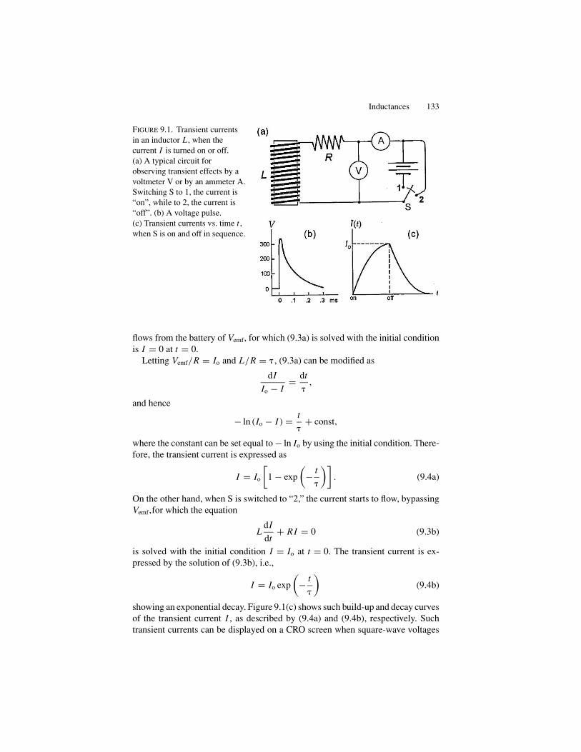
Inductances 133
FIGURE 9.1. Transient currentsin an inductor L , when thecurrent I is turned on or off.(a) A typical circuit forobserving transient effects by avoltmeter V or by an ammeter A.Switching S to 1, the current is“on”, while to 2, the current is“off”. (b) A voltage pulse.(c) Transient currents vs. time t ,when S is on and off in sequence.
flows from the battery of Vemf, for which (9.3a) is solved with the initial conditionis I = 0 at t = 0.
Letting Vemf/R = Io and L/R = � , (9.3a) can be modified as
dI
Io − I= dt
�,
and hence
− ln (Io − I ) = t
�+ const,
where the constant can be set equal to − ln Io by using the initial condition. There-fore, the transient current is expressed as
I = Io
[1 − exp
(− t
�
)]. (9.4a)
On the other hand, when S is switched to “2,” the current starts to flow, bypassingVemf,for which the equation
LdI
dt+ RI = 0 (9.3b)
is solved with the initial condition I = Io at t = 0. The transient current is ex-pressed by the solution of (9.3b), i.e.,
I = Io exp
(− t
�
)(9.4b)
showing an exponential decay. Figure 9.1(c) shows such build-up and decay curvesof the transient current I , as described by (9.4a) and (9.4b), respectively. Suchtransient currents can be displayed on a CRO screen when square-wave voltages
134 9. Inductances and Magnetic Energies
stimulate the on-off switching. We note that the parameter � is in units of sec andhence called the time constant of a given circuit.
If a high inductance L is connected with no resistance or a small R in the circuit,a high Vi surges when it is switched off, due to a large dI /dtand small time constant� , as shown in Figure 9.1(a). To avoid a dangerously high voltage surge in such acase, as a usual precaution one should include a sufficiently large R in series withthe circuit to maintain the current at a low level.
Next, we discuss such transient processes in terms of electrical energy. Equation(9.3a) multiplied by I is written as
L IdI
dt+ RI 2 = Vemf I,
where Vemf I expresses the power delivered by the battery. Integrating this equationfor a process of increasing current during the time interval between t = 0 to t = ∞,we obtain
1
2LI2
o +∫ ∞
0RI (t)2 dt = Vemf
∫ ∞
0I (t) dt,
signifying the energy relation among L , R and Vemf. Clearly, the term 1L I 2o in this
relationrepresents an energy stored in the inductor Lwhen it is activated by thecurrent Io, and the second term is the heat produced during the charging process.The magnetic energy can further be modified to express it by the field quantitiesB and H . Namely,
1
2LI2
o = 1
2
N2�2
L= N2 B2S2l
2�N2S= B2
2�Sl = umV, (9.5a)
where
um = B2
2�(9.5b)
is the energy density in the solenoid of volume V. For a general magnetic field,(9.5b) can be written as
um = 1
2�B2 = �
2H2 = 1
2B.H. (9.5c)
Example 1. Some numerical examples are instructive for understanding for-mal arguments. Referring to Figure 9.1, we assume that L = 3 henry andR = 20 ohm. If a battery of Vemf = 100 V is turned on at t = 0, thetransient current for activating L is characterized by the time constant� = L/R = 0.5 sec. The current is then given by I = Io[1 − exp(−t/0.5)],where Io = Vemf/R = 5 A. When t = � , then I = Io(1 – e−1) = 3.16 A,and dI/dt = 12.3 A/sec. Therefore, the magnetic energy increases at a rategiven by PL = d(1LI2)/dt = LI(dI/dt) = 3 henry × 3.16 A × 12.3 A/sec =17 watt. The heat dissipation in R occurs at a rate PR = I 2 R = (3.16 A)2 ×
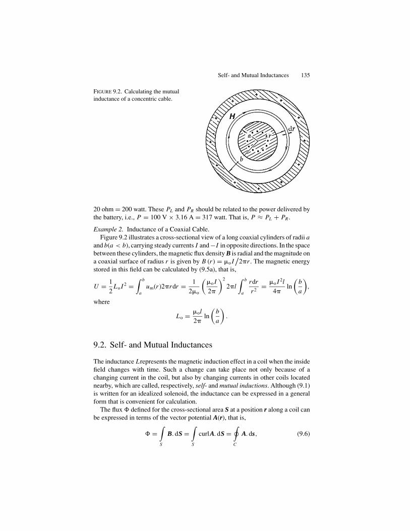
Self- and Mutual Inductances 135
FIGURE 9.2. Calculating the mutualinductance of a concentric cable.
20 ohm = 200 watt. These PL and PR should be related to the power delivered bythe battery, i.e., P = 100 V × 3.16 A = 317 watt. That is, P ≈ PL + PR .
Example 2. Inductance of a Coaxial Cable.Figure 9.2 illustrates a cross-sectional view of a long coaxial cylinders of radii a
and b(a < b), carrying steady currents I and −I in opposite directions. In the spacebetween these cylinders, the magnetic flux density B is radial and the magnitude ona coaxial surface of radius r is given by B (r ) = �o I
/2�r . The magnetic energy
stored in this field can be calculated by (9.5a), that is,
U = 1
2Lo I 2 =
∫ b
aum(r )2�rdr = 1
2�o
(�o I
2�
)2
2�l∫ b
a
rdr
r2= �o I 2l
4�ln
(b
a
),
where
Lo = �ol
2�ln
(b
a
).
9.2. Self- and Mutual Inductances
The inductance Lrepresents the magnetic induction effect in a coil when the insidefield changes with time. Such a change can take place not only because of achanging current in the coil, but also by changing currents in other coils locatednearby, which are called, respectively, self- and mutual inductions. Although (9.1)is written for an idealized solenoid, the inductance can be expressed in a generalform that is convenient for calculation.
The flux � defined for the cross-sectional area S at a position r along a coil canbe expressed in terms of the vector potential A(r), that is,
� =∫S
B. dS =∫S
curlA. dS =∮C
A. ds, (9.6)

136 9. Inductances and Magnetic Energies
where Stokes’s theorem was used for conversion from the surface to line integral,and ds is the line element on C . Considering a current j(r ′) at r ′, the potential A(r)at r is given by
A(r ) = �o
4�
∫v(r ′)
j(r ′)∣∣r − r ′∣∣d3r ′.
For the ring current along the coiled wire we can write j(r ′)d3r ′ = I ds′, and hence
A(r ) = �o I
4�
∮C
ds′
|r − r ′| .
Thus, from (9.6) we obtain the expression
L = �o
4�
∮C
∮C
ds.ds′
|r − r ′| . (9.7)
For two interacting coils 1 and 2 fluxes are written as
�1 =∮C1
(A11 + A12) . ds1 and �2 =∮C2
(A21 + A22) . ds2
where
A11 = �o I
4�
∮C1
ds′1∣∣r1 − r ′
1
∣∣ and A22 = �o I
4�
∮C2
ds′2∣∣r2 − r ′
2
∣∣are vector potentials due to inductions in these coils 1 and 2 by their own currentsI1 and I2, and
A12 = �o I
4�
∮C2
ds′2∣∣r1 − r ′
2
∣∣ and A21 = �o I
4�
∮C1
ds′1∣∣r2 − r ′
1
∣∣represent inductions mutually caused by I2 and I1, respectively.
Therefore we can write
�1 = L11 I1 + M12 I2 and �2 = M21 I1 + L22 I2, (9.8)
where
L11 = �o
4�
∮C1
∮C1
ds1.ds′1∣∣r1 − r ′1
∣∣ and L22 = �o
4�
∮C2
∮C2
ds2.ds′2∣∣r2 − r ′2
∣∣ (9.9)
are called self-inductances, and
M12 = �o
4�
∮C1
∮C2
ds1.ds′2∣∣r1 − r ′2
∣∣ and M21 = �o
4�
∮C2
∮C1
ds2.ds′1∣∣r2 − r ′1
∣∣ (9.10)

Self- and Mutual Inductances 137
the mutual inductances. We note that in (9.10) these mutual inductances are sym-metrical between 1 and 2, that is,
M12 = M21. (9.11)
Activated independently by currents I1 and I2, the two inductors interact mag-netically at a close distance. As discussed for a single inductor in Section 9.1,energies from two emfs are dissipated in resistances in part and stored, also, ininductors as magnetic energies. For two conductors the induced voltages are deter-mined by Vin(1) = −d�1/dt and Vin(2) = −d�2/dt , respectively, where �1 and�2 are given by (9.8). Therefore, the stored energy is expressed by
U (t) = −t∫
0
d�1
dtI1dt −
t∫0
d�2
dtI2dt .
Using (9.8), this can be written as
U (t) = 1
2L11 I 2
1 + 1
2L22 I 2
2 + M12 I1 I2 + M21 I2 I1, (9.12a)
varying generally as a function of time, as I1 and I2 change with different timeconstants. However, both currents become steady as t → ∞. With stationary cur-rents on, both inductors can store energies in the form 1L I 2
o , whereas symmetricalmutual inductances (M12 = M21) give rise to the same interaction energy. There-fore, the total magnetic energy in the two inductors with steady currents I1 and I2
can be expressed as
U (t) = 1
2L1 I 2
1 + 1
2L2 I 2
2 + M I1 I2, (9.12b)
which is the same as (9.12a) where L11, L22, and M12 = M21 are replaced by L1,L2, and M .
Self-inductance characterizes an inductor as a circuit element, while mutual in-ductance signifies a coupling between inductors, depending on their distance andarrangement. In the above we discussed two inductors activated individually by cur-rents I1and I2; however, in many cases these currents may originate from the samesource. A coaxial inductor is the example wherein the magnetic field exists onlyinside the coaxial cable as related to currents I andg − I on the inside and outsideconductors. Therefore, the inductance L calculated in Example 9.2 is the mutualinductance between the currents. Nevertheless, the mutual parameter M refers toan interaction between two well-defined inductors with a fixed configuration.
We can show that at any point in a magnetic field the energy density um isexpressed by (9.5c). In the above, A11 + A12 and A21 + A22 represent in partsthe vector potential A in the entire field at the positions of currents I1 and I2,respectively. Therefore, the rate at which magnetic energy changes is given by
dU (1, 2)
dt= I1
d�1
dt+ I2
d�2
dt= I1
d
dt
∮C1
A.ds + I2d
dt
∮C2
A.ds;
138 9. Inductances and Magnetic Energies
however, the mutual interactions are duplicated in this expression. Writing I1ds =j1dv, I2ds = j2dv, and j1 + j2 = j , for a symmetric energy U = 1
2[U (1, 2) +
U (2, 1)] we have
2dU
dt= d
dt
∫v
A. jdv = d
dt
∫v
A. curlHdv.
Using the identity div(A × H) = (curlA). H − A. (curlH), the last integral can beexpressed as∫
v
A. (curlH) dv =∫
v
(curlA) . Hdv −∫
v
div (A × H) dv.
Here, with the Gauss theorem, we have∫v
div (A × H) dv = ∮S (A × H)n dS → 0
as S → ∞, and therefore obtain the formula U = 12
∫v
B. Hdv for a stationary fieldwith the energy density um = 1
2 B. H.
9.3. Mutual Interaction Force Between Currents
We discussed the magnetic field of two current-activated inductors, where thestored energy is not only in individual coils, but also in the space in between. Theenergy of the field spread between inductors was calculated as in Section 9.2 fora rigid configuration.
On the other hand, in a non-rigid configuration the interaction energy W betweentwo inductors is responsible for a mechanical force. Such an interaction force canbe considered as arising from a variation in W due to a small displacement �r inthe mutual distance. Namely,
−F. �r = �W. (9.13)
Such a small variation �W in the interaction energy can occur with a variation inmagnetic flux, so that we can write
�W = I1��12 = I2��21,
where
��12 =∫
S1
B2(r1).�S1 =∫
S1
B2(r1). (ds1 × �r ) ={ ∮
C1
B2(r ) × ds1
}.�r .
and hence the force F12 can be determined by
F12 = I1
(∮C1
B2 (r1) × ds1
).
In this case, the Biot–Savart formula is written as
B2 (r1) = �o I2
4�
∮C2
ds2 × (r1 − r2)
|r1 − r2|3,

Examples of Mutual Induction 139
and therefore the interaction force can be expressed as
F12 = −F21 = �o I1 I2
4�
∮C1
ds1 ×∮C2
ds2 × (r1 − r2)
|r1 − r2|3. (9.14)
9.4. Examples of Mutual Induction
9.4.1. Parallel Currents
In Section 7.3, we discussed a magnetic force between parallel currents. Here wecalculate the mutual inductance and force with formulas (9.10) and (9.14).
Figure 9.3 shows two parallel conductors of finite length l and width d. Takingcurrent elements I1dz1 and I2dz2 at z1 and z2 on these conductors, as indicated inthe figure, we calculate the mutual inductance with (9.10). That is,
M = �o
4�
l∫0
dz1
l∫0
dz2√d2 + (z1 − z2)2
.
Replacing z2 by x = (z1– z2)/d, we have
l∫0
dz2√d2 + (z1 − z2)2
=(l−z1)/d∫−z1/d
dx√1 + x2
= sinh−1
(l − z1
d
)+ sinh−1
( z1
d
).
These terms on the right give rise to basically the same results as when the expres-sion is integrated once again, namely,
M = �o
4�2d
l/d∫0
(sinh−1 x
)dx = x sinh−1 x −
√1 + x2.
FIGURE 9.3. Calculating the mutual inductance of twin parallelcurrents.
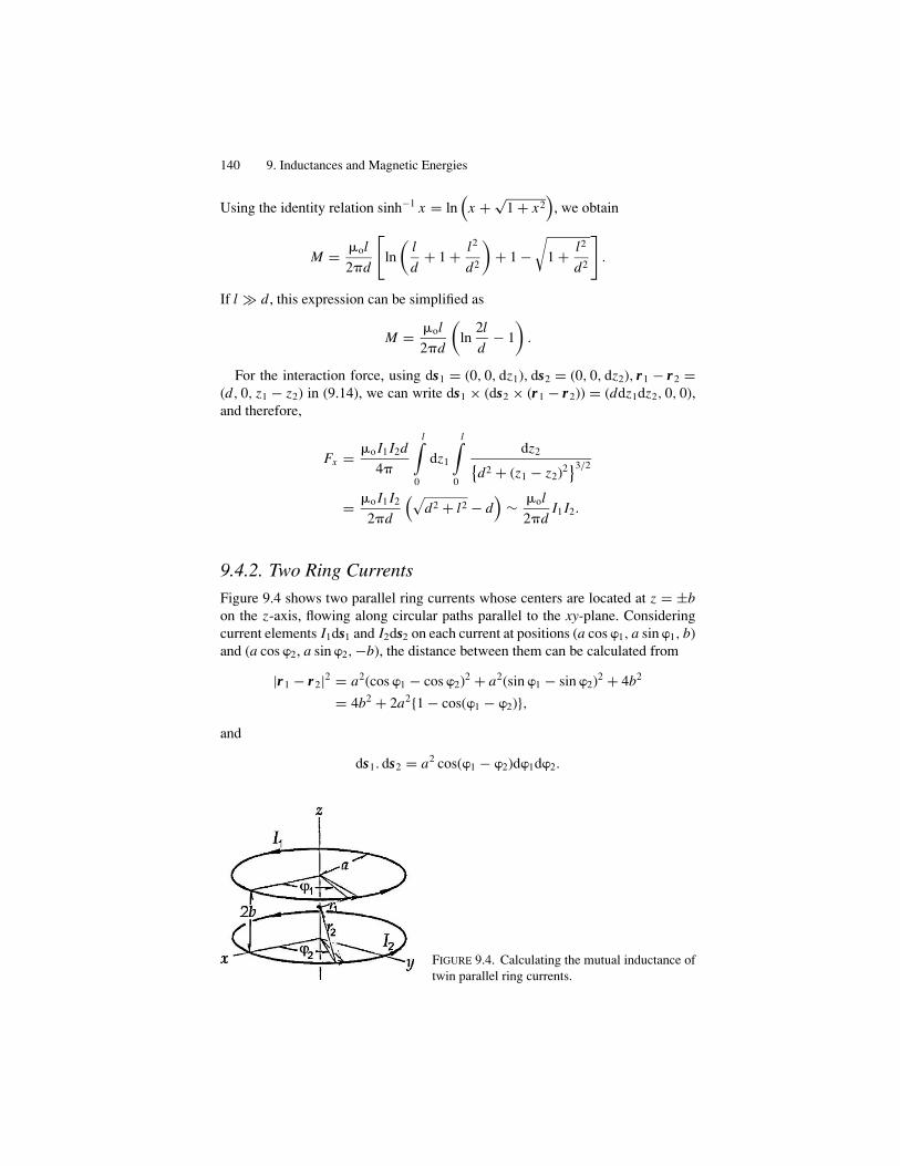
140 9. Inductances and Magnetic Energies
Using the identity relation sinh−1 x = ln(
x + √1 + x2
), we obtain
M = �ol
2�d
[ln
(l
d+ 1 + l2
d2
)+ 1 −
√1 + l2
d2
].
If l � d , this expression can be simplified as
M = �ol
2�d
(ln
2l
d− 1
).
For the interaction force, using ds1 = (0, 0, dz1), ds2 = (0, 0, dz2), r1 − r2 =(d, 0, z1 − z2) in (9.14), we can write ds1 × (ds2 × (r1 − r2)) = (ddz1dz2, 0, 0),and therefore,
Fx = �o I1 I2d
4�
l∫0
dz1
l∫0
dz2{d2 + (z1 − z2)2
}3/2
= �o I1 I2
2�d
(√d2 + l2 − d
)∼ �ol
2�dI1 I2.
9.4.2. Two Ring Currents
Figure 9.4 shows two parallel ring currents whose centers are located at z = ±bon the z-axis, flowing along circular paths parallel to the xy-plane. Consideringcurrent elements I1ds1 and I2ds2 on each current at positions (a cos �1, a sin �1, b)and (a cos �2, a sin �2, −b), the distance between them can be calculated from
|r1 − r2|2 = a2(cos �1 − cos �2)2 + a2(sin �1 − sin �2)2 + 4b2
= 4b2 + 2a2{1 − cos(�1 − �2)},and
ds1. ds2 = a2 cos(�1 − �2)d�1d�2.
FIGURE 9.4. Calculating the mutual inductance oftwin parallel ring currents.
Examples of Mutual Induction 141
Writing � = �1 − �2, the mutual inductance is a function of � and �2, but can beexpressed as
M = �o
4�
(2�a2) 2�∫
0
cos �d�√4b2 + 2a2 (1 − cos �)
,
after integrating with respect to �2. Further, defining an angle � = 12 (� − �), M
can be written in terms of elliptic complete integrals, as derived in the following:
cos � = 2 sin2 � − 1, 4b2 + 2a2(1 − cos �) = 4{b2 + a2(1 − sin2 �)},and the range of integration becomes − 1
2 � ≤ � ≤ 12 �. Thus, we obtain
M = �oa2
�/2∫0
(2 sin2 � − 1
)d�√
a2 + b2 − a2 sin2 �.
Define a parameter �2 = a2
a2 + b2, and splitting 2 sin2 � − 1 into two parts as
2 sin2 � − 1 = 2 − �2
�2− 2
(1 − �2 sin2 �
)�2
,
the last expression for M is divided into two terms of complete elliptic integrals,i.e.,
M = �oa2
�
[(2 − �2) K (�) − 2E (�)
],
where
K (�) =�/2∫0
d�√1 − �2 sin2 �
and E (�) =�/2∫0
√1 − �2 sin2 �d�
are known as complete elliptic integrals of the first and second kinds, respectively.

10Time-Dependent Currents
10.1. Continuity of Charge and Current
Static charges and steady currents are responsible for electrostatic and steadymagnetic fields, respectively. A static field arises from a charge Q at rest, whereas,for a steady field, a constant current I = dQ/dt is responsible; both representstates of the charge carriers relative to the observer. However, charge and currentare not exclusive, and both electric and magnetic fields can be observed as relatedwith time-dependent Q and I , as discussed for magnetic induction.
Referring to Figure 1.2, if a current I is not steady, not all charges in the volumeS�x are necessarily moving out during the time-interval �t , depending on theposition x along the conductor. For such a non-steady flow of charges, we can
write I (x) − I (x − �x) = �Q
�t, which can be expressed as
−� ( j S)
�x�x = ��
�tS�x, and hence − � j
�x= ��
�t. (10.1a)
In general, the charge density � and the current vector j are functions of the positionr and time t along the current passage for which (10.1a) can be expressed as
∂�
∂t+ div j = 0, (10.1b)
which is known as the equation for continuity. Obviously, (10.1b) signifies that� and j are not independent, so that these quantities, as combined, represent thesource of electromagnetic fields.
Assuming that all particles move at the same speed v in one-dimensional flow,we have j = �v, and the equation (10.1b) can be expressed as
∂�
∂t+ v
∂�
∂x= 0, (10.1c)
where � is a function of x and t . We assume that such a function � (x, t) is separableinto factor functions of x and t only, as given by a product � (x, t) = �1(x)�2(t).
142

Alternating Currents 143
Then, from (10.1c) we obtain
v
�1
d�1
dx= − 1
�2
d�2
dt= i�,
where � is a constant independent of x and t , ignoring frictional effects. Solvingfor �1 and �2, we can write
� (x, t) = �oexp{−i�
(t − x
v
)},
representing the propagating density � that can be specified by the phase
�(
t − x
v
), where the constant � is interpreted as the frequency of periodic vari-
ation. At a low frequency �− the phase is dominated by �t if�
vx is negligi-
ble in macroscopic scale. In this case, the specific solution of (10.1c) is givenby j = �v = �ovexp(−i�t), and the corresponding current can be expressed asI = Ioexp(−i�t), almost independent of x . In contrast, at a higher �, as signified
by the wavelength � = 2�v
�the term
�
vx becomes significant for the density to
propagate along x , and the current performance is seriously affected by the size andshape of a circuit. Leaving high-frequency problems to a later discussion, in thischapter we discuss time-dependent currents at low frequencies, occurring almostsimultaneously in the whole circuit.
10.2. Alternating Currents
The principle of generating alternating current (AC) was briefly discussed in Sec-tion 7.3 as an example of a magnetic force. By rotating a rectangular coil, as shownin Figure 7.7, around the axis placed in perpendicular to the direction of a staticmagnetic field, an induced voltage Vin occurs as described by the Faraday–Lenz
law, i.e., Vin = −d�
dt, where the magnetic flux is � = �o sin �, here � is the ro-
tational angle, i.e., � = �t + �o. Here �o is the initial angle at t = 0, and � is theangular frequency of rotation. Therefore, the induced voltage changes sinusoidallywith t , as given by
Vin = Vocos�, where Vo = −��o,
indicating that the amplitude Vo is proportional to �, and that the variation of Vin
is signified by the angle �, which is given by the phase of the alternating voltage.If such a voltage source is connected with a resistor R, an induction current I
flows as determined by the Ohm law, Vin = RI , and hence
I = Vo
Rcos (�t + �o) , (i)
which is in phase with Vin.
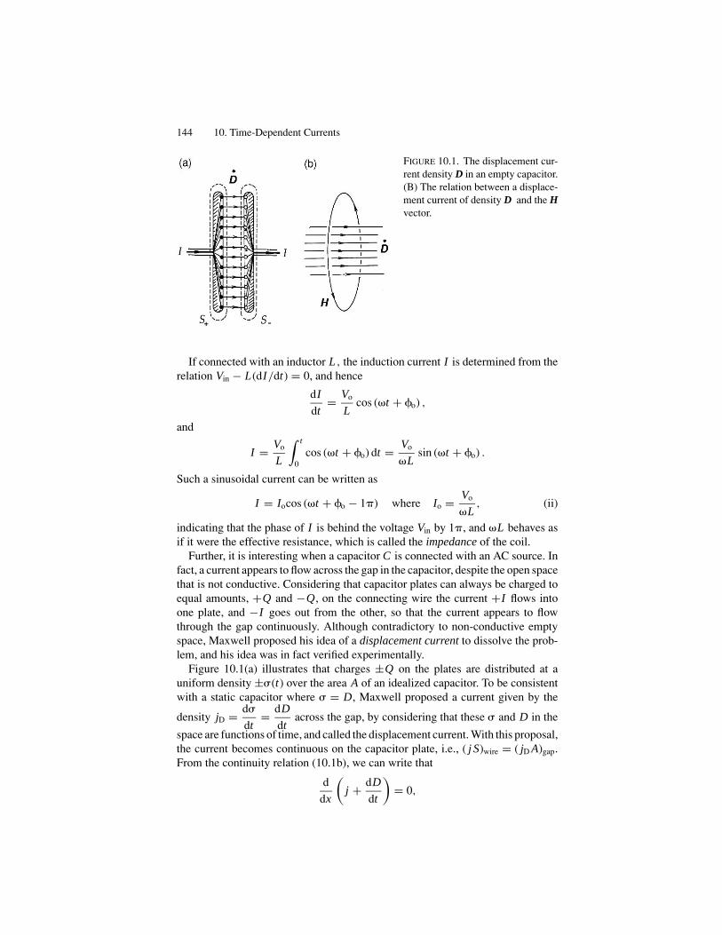
144 10. Time-Dependent Currents
FIGURE 10.1. The displacement cur-rent density D in an empty capacitor.(B) The relation between a displace-ment current of density D and the Hvector.
If connected with an inductor L , the induction current I is determined from therelation Vin − L(dI/dt) = 0, and hence
dI
dt= Vo
Lcos (�t + �o) ,
and
I = Vo
L
∫ t
0cos (�t + �o) dt = Vo
�Lsin (�t + �o) .
Such a sinusoidal current can be written as
I = Iocos (�t + �o − 1�) where Io = Vo
�L, (ii)
indicating that the phase of I is behind the voltage Vin by 1�, and �L behaves asif it were the effective resistance, which is called the impedance of the coil.
Further, it is interesting when a capacitor C is connected with an AC source. Infact, a current appears to flow across the gap in the capacitor, despite the open spacethat is not conductive. Considering that capacitor plates can always be charged toequal amounts, +Q and −Q, on the connecting wire the current +I flows intoone plate, and −I goes out from the other, so that the current appears to flowthrough the gap continuously. Although contradictory to non-conductive emptyspace, Maxwell proposed his idea of a displacement current to dissolve the prob-lem, and his idea was in fact verified experimentally.
Figure 10.1(a) illustrates that charges ±Q on the plates are distributed at auniform density ±�(t) over the area A of an idealized capacitor. To be consistentwith a static capacitor where � = D, Maxwell proposed a current given by the
density jD = d�
dt= dD
dtacross the gap, by considering that these � and D in the
space are functions of time, and called the displacement current. With this proposal,the current becomes continuous on the capacitor plate, i.e., ( j S)wire = ( jD A)gap.From the continuity relation (10.1b), we can write that
d
dx
(j + dD
dt
)= 0,

Impedances 145
which can be generalized as div
(j + ∂ D
∂t
)= 0. Maxwell considered that the net
current density j + ∂ D∂t
is responsible for the magnetic field H, and wrote the
Ampere law as
j + ∂ D∂t
= curl H. (10.2)
This is one of the Maxwell equations governing entire electromagnetic phenomena.Figure 10.1(b) shows the right-hand relation between ∂D/∂t and H vectors.
Returning to a capacitor connected with an AC generator, we have a voltagerelation
Vin = Q
C= 1
C
∫ t
0I dt = Vocos(�t + �o).
Differentiating this, we obtain
I = −Iosin(�t + �o) = Iocos
(�t + �o + 1
2�
), where Io = �CV o. (iii)
Therefore, the phase of AC current is advanced from that of Vin by1
2�, and the
impedance of a capacitor is given by 1/�C .
10.3. Impedances
A practical AC circuit consists of resistances, inductances, and capacitances con-nected in various ways with an AC source. Figures 10.2(a), (b), and (c) show
FIGURE 10.2. Impedances of AC cir-cuits in a complex plane. The phase� of AC current can delay or advancefrom the applied voltage. (a) RC, (b)RL, and (c) RCL combinations.

146 10. Time-Dependent Currents
simple cases of RC, RL, and RCL connected in series with Vin, respectively. In thefirst case, the voltage relation can be written as
Vin = RI + Qplate
C= RI + 1
C
∫ t
0IDdt, where I = ID,
Hence, the equation for I is given by
−�Vosin(�t + �o) = RdI
dt+ I
C.
Letting I = Iosin(�t + �o), the right side can be expressed by
RdI
dt+ I
C= �RIocos(�t + �o) + Io
Csin (�t + �o) ;
therefore we obtain the relation
−Vo cos (�t + �o) = RIo cos (�t + �o) + Io
�Csin (�t + �o)
= −√
R2 +(
1
�C
)2
Io cos (�t + �o − � ) , (iv)
where tan � = 1/�CR. The result can be expressed as
Vin = Z (�)I, I = Iocos(� + �o − � )
and
Z (�) =√
R2 + 1
�2C2= Vo
Io. (10.3a)
Here, the phase of I shows delay by � , and Z (�) is the impedance.In the case of RL shown in Figure 10.2(b), we can carry out a calculation similar
to the one above. The equation for the current is
Vo cos (�t + �o) − LdI
dt= RI,
which can be solved by letting I = Iocos(�t + �o). We obtain the relation
Vo cos(�t + �o) = �L Io sin (�t + �o) + RIo cos (�t + �o)
=√
R2 + (�L)2 Io cos (�to + �o + � ) , (v)
where tan � = R/�L . Therefore, we can define the impedance as
Z (�) =√
R2 + �2L2, (10.3b)
and the angle � represents the current phase, which advances the AC voltage.For the LCR case shown in Figure 10.2(c), we have the equation
Vo cos (�t + �o) − LdI
dt= Q
C+ RI,
which can be solved in similar manner, and the result is
Vo cos (�t + �o) = Z (�) Io cos (�t + �o − � ) ,

Complex Vector Diagrams 147
where
Z (�) =√
R2 +(
�L − 1
�C
)2
and tan � =�L − 1
�CR
. (10.3c)
The power delivered instantaneously by an AC source is expressed by
P (t) = V (t) I (t) = Vo Io cos � cos (� − � ) ,
where � = �t + �o is the voltage phase. However, for usual measurements withmeters it is convenient to define its average over a period of the AC cycle To =2�/�; that is,
〈P〉 = 1
To
∫ To
0Pdt = Vo Io
�
2�
∫ To
0cos � cos (� − � ) dt = 1
2Vo Io cos � .
(10.4)Accordingly, the AC voltage and current are defined as square roots of the mean-
square averages of V (t) and I (t), i.e. V =√⟨
V 2⟩ = Vo√
2and I = Io√
2, respec-
tively. With these mean-square roots, (10.4) can be expressed as 〈P〉 = V I cos � .It is noted that such averages are referred to conventional AC measurements overrepeated periods of oscillation, which are characterized by a long timescale ofobservation.
10.4. Complex Vector Diagrams
Equations (iv) and (v) indicate that AC voltages across R, L , and C can be giveneffectively as if these elements are connected individually with Vin, namely, RI, �LI,and I /�C , respectively. Further, (10.3a) and (10.3b) imply that the impedances canbe geometrically determined in x, y-planes by points (R, �L) and (R, −1/�C),where � is clearly the angle between the impedance Z and the x-axis, as illustratedin Figures 10.2(a) and (b). Equation (10.2c) can be interpreted that Z is represented
by a point
(R, �L − 1
�C
)and an angle � , as in Figure 10.2(c).
It is convenient to express such impedances on a complex plane, considering they-axis to be the imaginary axis iy. Actually, the diagrams shown in Figures 10.2(a),(b), and (c) are complex planes. Thus, the impedance can be expressed as a complexfunction of �, that is
Z (�) = R + i X (�), (10.5)
where the imaginary part X (�) is called the reactance, e.g., X (�) = �L − 1
�Cin
Figure 10.2(c).The vector-diagram method can also be obtained by considering the AC voltage
and current as complex variables, whose real parts represent actual variables. For
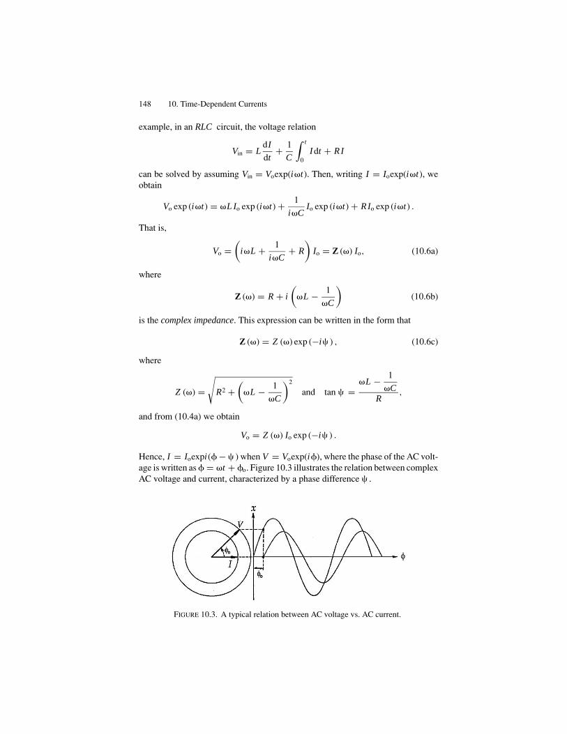
148 10. Time-Dependent Currents
example, in an RLC circuit, the voltage relation
Vin = LdI
dt+ 1
C
∫ t
0I dt + RI
can be solved by assuming Vin = Voexp(i�t). Then, writing I = Ioexp(i�t), weobtain
Vo exp (i�t) = �L Io exp (i�t) + 1
i�CIo exp (i�t) + RIo exp (i�t) .
That is,
Vo =(
i�L + 1
i�C+ R
)Io = Z (�) Io, (10.6a)
where
Z (�) = R + i
(�L − 1
�C
)(10.6b)
is the complex impedance. This expression can be written in the form that
Z (�) = Z (�) exp (−i� ) , (10.6c)
where
Z (�) =√
R2 +(
�L − 1
�C
)2
and tan � =�L − 1
�CR
,
and from (10.4a) we obtain
Vo = Z (�) Io exp (−i� ) .
Hence, I = Ioexpi(� − � ) when V = Voexp(i�), where the phase of the AC volt-age is written as � = �t + �o. Figure 10.3 illustrates the relation between complexAC voltage and current, characterized by a phase difference � .
FIGURE 10.3. A typical relation between AC voltage vs. AC current.

Resonances 149
10.5. Resonances
10.5.1. A Free LC Oscillation
In a circuit shown in Figure 10.4(a), when the switch S is turned on “1,” theinductor L becomes active with a current I . Switching S to “2” disconnects thebattery, and the capacitor C is charged to ±Q, which is then discharged throughL , then charges C , and continues repeatedly. As illustrated in Figure 10.4(b), suchan oscillation takes place in a cycle of 1-2-3-4 for a long time if the resistance ofthe coil is negligibly small.
A free oscillation between an idealized inductor and capacitor can be describedby
Vin = VC or − LdI
dt= Q
C.
Multiplying by I = dQ/dt , we have −L IdI
dt= Q
C
dQ
dt, which can then be inte-
grated with respect to time, that is,
1
2L I 2 + 1
2
Q2
C= const., (10.7a)
implying that the magnetic energy in the inductor is added to the electrostaticenergy in the capacitor in a given time t . Equation (10.7a) represents the energy ofa harmonic oscillation of (Q, I ), analogous to a mass particle, in which 1
2 L I 2 andQ2/2C signify kinetic and potential energies of the moving charge, respectively.
FIGURE 10.4. Free oscillation in anL − C circuit. (a) The inductor L isactivated when the switch S is turnedonto 1, and then to 2 for oscillation.(b) Repeated charging of the capaci-tor in sequence of 1-2-3-4-1.
150 10. Time-Dependent Currents
The characteristic frequency of oscillation can be expressed as
�o = 1√LC
, (10.7b)
and Q(t) = Qoexp(i�ot), I (t) = i�oQoexp(i�ot), where Qo is the amplitude,
shifting the current phase by1
2� .
10.5.2. Series Resonance
Consider a series of RCL connected with an AC source, as shown in Figure 10.2(c).In this case, the voltage-current relation is given by (10.6a), (b), and (c). It is notedthat if the frequency of AC voltage is equal to �o given by (10.7b), the reactanceX (�) vanishes at � = �o, i.e. X (�o) = 0, signifying that Z (�o) = R is minimum.The AC current exhibits maximum amplitude at this condition, which is thereforecalled the resonance.
At resonance the current and charge in the inductor and capacitor are in oscilla-tory motion with maximum amplitude at �o, while their energy is being dissipatedin the resistor. Hence, the resonance quality can be expressed by the ratio betweenthe energies of oscillation and dissipation averaged over a cycle of oscillation, i.e.,
�oL
⟨I 2
⟩R
⟨I 2
⟩ = �oL
R= 1
Qo, (10.8)
where Qo is called the quality factor or Q-factor of resonance.The reactance X (�) can be modified by using the definitions of �o and Qo given
by (10.7b) and (10.8) as
X (�) = RQo
(�
�o− �o
�
),
and, hence, the impedance is expressed as
Z (�)2 = R2 + X (�)2 = R2
{1 + Q2
o
(�
�o− �o
�
)2}
.
Therefore, currents at off- and on resonance can be calculated as Io(�) = Vo/Z (�)and Io(�o) = Vo/R, respectively, for which we have the formula,
Io (�)2
Io (�o)2 = 1
1 + Q2o
(�
�o− �o
�
)2 . (10.9a)
Figure 10.5 sketches the curve of (10.9a) against��/�o, where±�� = � − �o. In
such a curve, frequencies �± at half-power points, defined by Io(�±)2/Io(�o)2 = 1
2,
are of particular interest. Writing �± = �o ± ��,�±�o
− �o
�±∼= ±2��±
�o, and

Resonances 151
FIGURE 10.5. A typical L-Cresonance. The half-width isindicated as 1/Qo, where thequality factor Qo depends onthe internal resistance R in theinductor L .
from the relation 1 + 4Q2o
(��±
�o
)2
= 2, we obtain
2��±�o
= 1
Qo. (10.9b)
The quality factor Qo can be easily estimated from half-power points, as shownin the figure.
10.5.3. Parallel Resonance
Figure 10.6 shows a parallel connection of L and C , where the resistance R canrepresent an internal resistance in L as well as added resistances, for which theKirchhoff rules may be applied as in a DC circuit. With regard to junctions, markeda and b in the figure, the impedances R + i�L and 1/i�C are connected in parallel,for which the voltage difference Vab is expressed as
Vab = (R + i�L) I1 = 1
i�CI2,
FIGURE 10.6. A circuit for L-C resonance. Nor-mally, R represents the internal resistance due to afinite conductivity of the coil.
152 10. Time-Dependent Currents
where I1 + I2 = I is the net current to satisfy Vin = Z (�)I . Therefore,
I = Vab
R + i�L+ i�CVab = Y (�)Vab,
where Y (�) is the complex admittance
Y (�) = 1
R + i�L+ i�C = R − i�L
R2 + �2L2+ i�C.
In this case, the resonance is signified by a particular frequency �o for the imaginary
part to become zero, that is,L
R2 + �2o L2
− C = 0, in which case the resonance
frequency is determined by
�2o = 1
LC− R2
L2, (10.10)
giving the characteristic frequency identical to (10.7b) in a series resonance, pro-vided R is negligible. However, the impedance at resonance can be written as
Z (�o) = V (�o)
I (�o)= R2 + �2
o L2
R= L
C R,
for which an internal resistance R cannot be considered zero. Nevertheless, if soassumed, I (�o) = 0 and I1(�o) = −I2(�o), so that the parallel resonance is oftenreferred to as anti-resonance.
In practice, for a parallel resonator characterized by L and C , 1/√
LC is a usefulparameter for approximate resonance. We can therefore write an approximaterelation between the exact resonance frequency o and �o = 1/
√LC , with which
(10.8) can be re-expressed as
2o = �2
o
(1 − 1
Q2o
)where
1
Qo= �oL
R.
Therefore,
o ≈ �o
(1 − 1
2Q2o
)and Z (o) ≈ Z (�o)
(1 + 1
Q2o
).
10.6. Four-Terminal Networks
In this section, we discuss circuits with two input and two output terminals, knowngenerally as a four-terminal networks. When an AC voltage is applied to an input,the output voltage is not necessarily sinusoidal, as caused by relaxation effectswith resistive elements. A guiding principle for solving network problems is theKirchhoff rules at low frequencies, thereby considering a unique time-dependentpotential at each point in a given circuit as related to the input phase. As willbe discussed in Chapter 11 for high frequencies, this assumption is valid only atsufficiently low frequencies, where the physical size of a circuit is smaller than awavelength of radiation.

Four-Terminal Networks 153
FIGURE 10.7. A simple four-terminal network. The input andoutput are 1-2 and 3-4, respectively.
10.6.1. RC Network
Figure 10.7 shows a circuit of C and R connected in series, where terminals 1and 2 constitute the input, to which a varying voltage can be applied. The outputterminals 3 and 4 are “open,” meaning unloaded, while we assume that terminals1 and 3 are connected to the “ground,” i. e., V1 = V3 = 0.
We first calculate the output voltage V4 at the open terminal 4, when an AC volt-age at a frequency � is applied to the input. The voltage relation can be written as
V2 − V4 = Q
Cand V4 = RI.
Writing the input voltage as V2 = V (t), we have
I = Cd (V2 − V4)
dt= V4
R.
Therefore, the differential equation for V4 is given by
dV4
dt+ V4
= dV2
dt, (10.11)
where = RC is the time constant. For a sinusoidal input V2 = Voexp(i�t), wecan set V4 = V4oexp(i�t) in (10.11) and obtain(
i� + 1
)V4o = i�Vo,
and hence
V4o
Vo= i�
1 + i�= i� (1 − i� )
1 + �2 2
= �√1 + �2 2
i + �√1 + �2 2
= �√1 + �2 2
exp i�,
where tan � = 1
�. Therefore, the output voltage is given by
V4 = Vo�√1 + �2 2
exp i(�t + �) , (10.12)
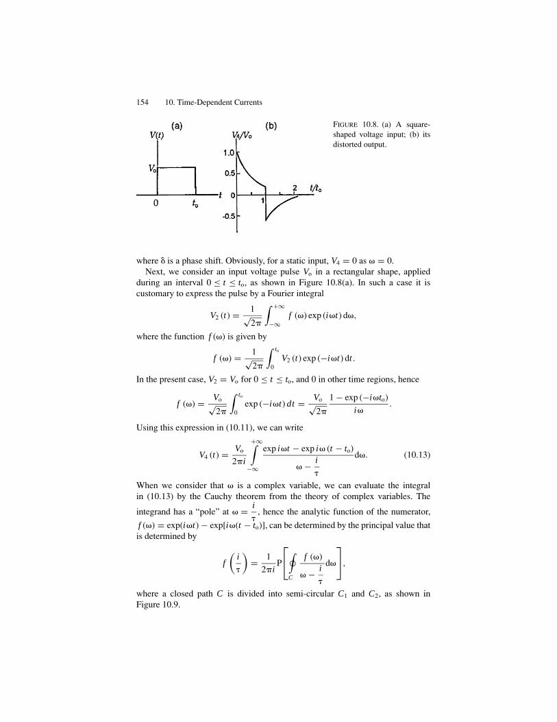
154 10. Time-Dependent Currents
FIGURE 10.8. (a) A square-shaped voltage input; (b) itsdistorted output.
where � is a phase shift. Obviously, for a static input, V4 = 0 as � = 0.Next, we consider an input voltage pulse Vo in a rectangular shape, applied
during an interval 0 ≤ t ≤ to, as shown in Figure 10.8(a). In such a case it iscustomary to express the pulse by a Fourier integral
V2 (t) = 1√2�
∫ +∞
−∞f (�) exp (i�t) d�,
where the function f (�) is given by
f (�) = 1√2�
∫ to
0V2 (t) exp (−i�t) dt .
In the present case, V2 = Vo for 0 ≤ t ≤ to, and 0 in other time regions, hence
f (�) = Vo√2�
∫ to
0exp (−i�t) dt = Vo√
2�
1 − exp (−i�to)
i�.
Using this expression in (10.11), we can write
V4 (t) = Vo
2�i
+∞∫−∞
exp i�t − exp i� (t − to)
� − i
d�. (10.13)
When we consider that � is a complex variable, we can evaluate the integralin (10.13) by the Cauchy theorem from the theory of complex variables. The
integrand has a “pole” at � = i
, hence the analytic function of the numerator,
f (�) = exp(i�t) − exp[i�(t − to)], can be determined by the principal value thatis determined by
f
(i
)= 1
2�iP
⎡⎣∮
C
f (�)
� − i
d�
⎤⎦,
where a closed path C is divided into semi-circular C1 and C2, as shown inFigure 10.9.
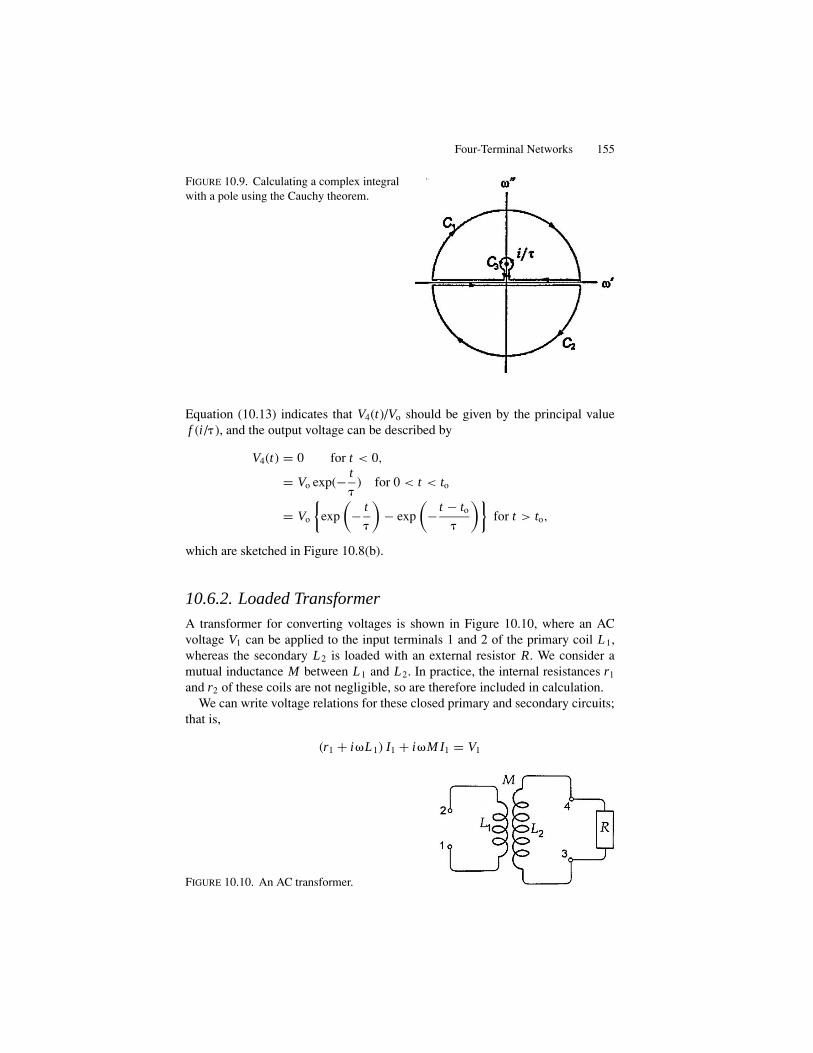
Four-Terminal Networks 155
FIGURE 10.9. Calculating a complex integralwith a pole using the Cauchy theorem.
Equation (10.13) indicates that V4(t)/Vo should be given by the principal valuef (i / ), and the output voltage can be described by
V4(t) = 0 for t < 0,
= Vo exp(− t
) for 0 < t < to
= Vo
{exp
(− t
)− exp
(− t − to
)}for t > to,
which are sketched in Figure 10.8(b).
10.6.2. Loaded Transformer
A transformer for converting voltages is shown in Figure 10.10, where an ACvoltage V1 can be applied to the input terminals 1 and 2 of the primary coil L1,whereas the secondary L2 is loaded with an external resistor R. We consider amutual inductance M between L1 and L2. In practice, the internal resistances r1
and r2 of these coils are not negligible, so are therefore included in calculation.We can write voltage relations for these closed primary and secondary circuits;
that is,
(r1 + i�L1) I1 + i�M I1 = V1
FIGURE 10.10. An AC transformer.
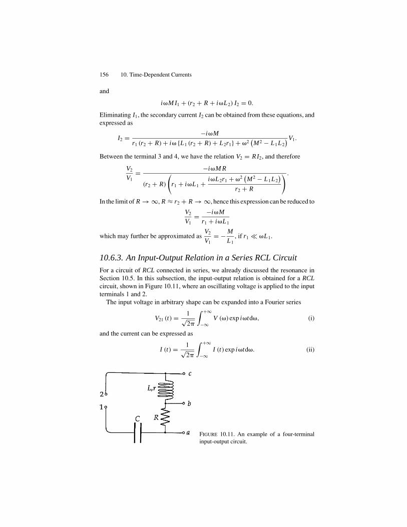
156 10. Time-Dependent Currents
and
i�M I1 + (r2 + R + i�L2) I2 = 0.
Eliminating I1, the secondary current I2 can be obtained from these equations, andexpressed as
I2 = −i�M
r1 (r2 + R) + i� {L1 (r2 + R) + L2r1} + �2(M2 − L1L2
) V1.
Between the terminal 3 and 4, we have the relation V2 = RI2, and therefore
V2
V1= −i�M R
(r2 + R)
(r1 + i�L1 + i�L2r1 + �2
(M2 − L1L2
)r2 + R
) .
In the limit of R → ∞, R ≈ r2 + R → ∞, hence this expression can be reduced to
V2
V1= −i�M
r1 + i�L1
which may further be approximated asV2
V1= − M
L1, if r1 �L1.
10.6.3. An Input-Output Relation in a Series RCL Circuit
For a circuit of RCL connected in series, we already discussed the resonance inSection 10.5. In this subsection, the input-output relation is obtained for a RCLcircuit, shown in Figure 10.11, where an oscillating voltage is applied to the inputterminals 1 and 2.
The input voltage in arbitrary shape can be expanded into a Fourier series
V21 (t) = 1√2�
∫ +∞
−∞V (�) exp i�td�, (i)
and the current can be expressed as
I (t) = 1√2�
∫ +∞
−∞I (t) exp i�td�. (ii)
FIGURE 10.11. An example of a four-terminalinput-output circuit.

Four-Terminal Networks 157
The voltage relation is
V21 − LdI
dt= (R + r ) I + Q
C,
from which the equation to be solved for I (t) is
d2 I
dt2+ (R + r )
dI
dt+ 1
CI = dV21
dt. (iii)
This is a linear differential equation, and (ii) is a linear combination of sinusoidalfunctions exp(i�t) indexed by �. Therefore, we can derive from (iii) solutionswith respect to individual �. Using the series (i) and (ii) in the equation (iii), foreach component at � we obtain{
−�2L + i� (R + r ) + 1
�C
}I (�) = i�V (�) ,
and hence
I (�) = V (�)
R + r + i
(�L − 1
�C
) .
The output voltage between the terminals c and b in Figure 10.10, is given by
Vcb = 1√2�
∫ +∞
−∞(r + i�L) I (�) exp(i�t)d�,
whereas those between b-a and a-1 are
Vba = 1√2�
∫ +∞
−∞RI (�) exp(i�t)d�
and
Va1 = 1√2�
∫ +∞
−∞
I (�)
Cexp(i�t)d�.
At resonance, i.e., � = �o = 1/√
LC , these output voltages are signified by thecurrent, i.e., I (�o)exp(−i� ), where the phase shift � is determined by
tan � = 1
R + r
(�L − 1
�C
).
10.6.4. Free Oscillation in an RCL Circuit
In an unloaded RCL circuit, as shown in Figure10.11, we consider a free oscillationcaused by a short voltage pulse applied to 1 and 2.
An input pulse is assumed as a voltage Vo in a short duration of time , beingdescribed by a delta function, i.e., Vin = Vo�( ). The current in the circuit is givenin such a Fourier series as (ii) in the previous subsection, hence,
Vin (t) = Vo
2�
∫ +∞
−∞exp(i�t)d�,
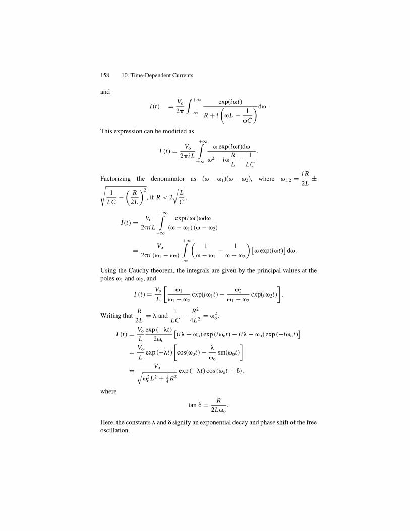
158 10. Time-Dependent Currents
and
I (t) = Vo
2�
∫ +∞
−∞
exp(i�t)
R + i
(�L − 1
�C
)d�.
This expression can be modified as
I (t) = Vo
2�i L
+∞∫−∞
� exp(i�t)d�
�2 − i�R
L− 1
LC
.
Factorizing the denominator as (� − �1)(� − �2), where �1,2 = i R
2L±√
1
LC−
(R
2L
)2
, if R < 2
√L
C,
I (t) = Vo
2�i L
+∞∫−∞
exp(i�t)�d�
(� − �1) (� − �2)
= Vo
2�i (�1 − �2)
+∞∫−∞
(1
� − �1− 1
� − �2
) [� exp(i�t)
]d�.
Using the Cauchy theorem, the integrals are given by the principal values at thepoles �1 and �2, and
I (t) = Vo
L
[�1
�1 − �2exp(i�1t) − �2
�1 − �2exp(i�2t)
].
Writing thatR
2L= � and
1
LC− R2
4L2= �2
o,
I (t) = Vo
L
exp (−�t)
2�o
[(i� + �o) exp (i�ot) − (i� − �o) exp (−i�ot)
]
= Vo
Lexp (−�t)
[cos(�ot) − �
�osin(�ot)
]
= Vo√�2
o L2 + 14 R2
exp (−�t) cos (�ot + �) ,
where
tan � = R
2L�o.
Here, the constants � and � signify an exponential decay and phase shift of the freeoscillation.

Part 3Electromagnetic Waves
159

11Transmission Lines
11.1. Self-Sustained Oscillators
Free oscillation in a circuit is generally short-lived because of the presence of aresistance. Normally AC current flows continuously, as the generator keeps supply-ing energy, but it is not simple to obtain a source of persisting electrical oscillationsat a desired frequency. Today, vacuum tubes and semi-conducting devices, oscil-lators, signal amplifiers, and other electronically controlled circuits are availableat almost any frequency, thereby, basic electromagnetic experiments can be per-formed with precision in modern electronics. A self-sustaining oscillator with asizable output power is a particularly important device to study high-frequencyphenomena.
A sustaining oscillator is basically a forced oscillator whose output power is fedback in part to the input to sustain oscillation. In this section, to understand thefeedback principle, we take a vacuum tube as an example, although it is almostobsolete in modern electronics. In fact, a feedback mechanism is significant forvarious growing processes in natural phenomena, and described effectively interms of negative resistance in circuit theory. While a conventional (positive)resistance signifies energy loss, a negative resistance can be interpreted as sustainedoscillation.
Figure 11.1(a) shows a circuit of a triode tube providing an electronically gener-ated current I (t) at the characteristic frequency �o determined by the LC resonator.The triode consists of an electron-emitting cathode (K), an anode (A), and a grid(G) that controls the electronic flow in the tube. The electronic current driven bythe anode voltage Va can be modified by the grid voltage Vg, exhibiting, typically,a sharp rise at a negative value of Vg = −Vb, called a bias voltage, as illustratedin Figure 11.1(b). In such a four-terminal circuit, the current-voltage relation cannormally be described by a linear relation
I = Y (�Va + Vg),
where Y is the electronic admittance and � the coupling between anode- and gridvoltages. In this case the output voltage is given by V = �Va + Vg, and the current
161

162 11. Transmission Lines
FIGURE 11.1. (a) A triode oscillator. (b) A typical non-linear I − V character.
modulated by the grid voltage �Vg, can be expressed by
�I = Y
(�
∂Va
∂Vg+ 1
)�Vg = (−��o + 1) �Vg,
where �o = −∂Va/∂Vg is called the amplification factor. Hence,
�Vg
�I= 1
Y (1 − ��o),
which is positive if 0 < ��o < 1, but negative if ��o > 1. The former case repre-sents an amplification, whereas the latter condition gives rise to a negative resis-tance for the current to be controlled by the bias potential. In solid state electronicsthe I -V relation in some semi-conductors is signified by a negative slope in a cer-tain region as shown in Figures 11.2(a) and (b). This condition provides a negativedamping condition similar to a triode case.
Electric oscillations in a wide range of frequencies are utilized for a variety ofapplications, such as telecommunications and other purposes in modern electronicsfor which oscillators are built on the basis of the principle of negative feedback.Although no details of oscillating mechanisms are given here, we should bearin mind in the following discussions that self-sustaining oscillators are alwaysinvolved in interpreting theoretical results.
FIGURE 11.2. Examples for neg-ative resistances.

Transmission Lines 163
11.2. Transmission Lines
Long parallel wires and concentric conductors are of particular importance for sig-nal transmission. Known as Lecher’s wires and coaxial cable, these transmissionlines are mathematically equivalent, sharing similar principles. Physically, how-ever, their performances are not identical: the electromagnetic field is completelyconfined to the space of a coaxial cable, whereas it is somewhat diffused fromLecher’s wires. Both devices are in practical use, but a coaxial cable is an idealtransmission line at high frequencies. Practically, the space between two conduc-tors is filled with insulating material to maintain uniform spacing, although thesignal can be modified by the dielectric property. At a high frequency, the oscillatorenergy is transferred to such a transmission line, thus it is transferred to a terminalload that is expressed by an impedance ZL, as illustrated in Figure 11.3.
In such a long device required for power transmission or communication pur-poses, the internal resistance cannot be ignored, and the capacitance between twoconductors plays an important role. Besides, their self- and mutual inductances arealso significant at high frequencies. Under the circumstances the voltage differenceacross the conductors and the currents on two conductors should be described asfunctions of the position x and time t , to which an oscillator and a terminal loadare connected.
For a uniform transmission line a potential difference �V between x andx + dx along the line should be related to a resistance R�x by the Ohm law�V = (R�x)�Icon, where R is defined as the resistance per unit length, andthe conduction current is �Icon = I (x + �x) − I (x). Writing for convenienceG�x = 1/R�x , where G is the conductance per unit length, we obtain the relation
Icon = (G�x)�V .
FIGURE 11.3. (a) Distributed impedances of a transmission line and a terminal impedanceZL. (b) Current and voltage functions. (c) Measuring VSWR in a transmission line.

164 11. Transmission Lines
Next, with regard to capacitive effect, the potential difference �V across thetwo conductors due to varying time can be expressed as �V = �Q/C�x , where
C represents the capacity per unit length. Hence, writing as �V = ∂ (�V )
∂t�t and
�Q = �Icap�t , we have
�Icap = �Q
�t= C�x
∂ (�V )
∂t.
Here, �Icap represents displacement current between the conductors. Therefore,on each conductor of the line we connect a loop of a net current I = Icon + Icap,
whose variation along the section �x is given by �Icon + �Icap = �I = ∂ I
∂x�x .
If such a line segment is isolated, �Icon = −�Icap, so that �I = 0. However, thepropagating current is signified by �I �= 0, which is ±�I or ∓�I , due to thecontinuity theorem, in opposite directions on each conducting segment.
On the other hand, the voltage relation in the loop must be �V + �V = 0, sothat
�V = −�V . (11.1)
Accordingly, we have
∂ I
∂x= −G�V − C
∂ (�V )
∂t,
which is the relation between the voltage difference �V (x, t) and currents ±I (x, t).Writing V (x, t) = �V for the potential difference between two conductors at x andt , this relation can be expressed as
∂ I
∂x= −GV − C
∂V
∂t, (11.2)
representing the voltage across the conductor V (x, t) and the conducting currents±I (x, t) along the transmission line.
For∂V
∂xon the two conductors we can write
∂V
∂x= −R (+I ) − L
∂ (+I )
∂t− M
∂ (−I )
∂t
and
−∂V
∂x= −R (−I ) − L
∂ (−I )
∂t− M
∂ (+I )
∂t,
where L and M are self- and mutual inductances per unit length. Combining theserelations, we can write
∂V
∂x= −RI − (L − M)
∂ I
∂t,
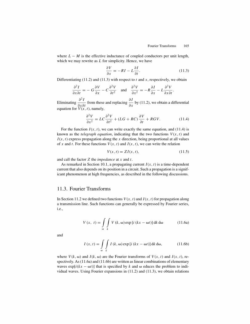
Fourier Transforms 165
where L − M is the effective inductance of coupled conductors per unit length,which we may rewrite as L for simplicity. Hence, we have
∂V
∂x= −RI − L
∂ I
∂t. (11.3)
Differentiating (11.2) and (11.3) with respect to t and x , respectively, we obtain
∂2 I
∂x∂t= − G
∂V
∂x− C
∂2V
∂t2and
∂2V
∂x2= −R
∂ I
∂x− L
∂2V
∂x∂t.
Eliminating∂2 I
∂x∂tfrom these and replacing
∂ I
∂xby (11.2), we obtain a differential
equation for V (x, t), namely,
∂2V
∂x2= LC
∂2V
∂t2+ (LG + RC)
∂V
∂t+ RGV . (11.4)
For the function I (x, t), we can write exactly the same equation, and (11.4) isknown as the telegraph equation, indicating that the two functions V (x, t) andI (x, t) express propagation along the x direction, being proportional at all valuesof x and t . For these functions V (x, t) and I (x, t), we can write the relation
V (x, t) = Z I (x, t), (11.5)
and call the factor Z the impedance at x and t .As remarked in Section 10.1, a propagating current I (x, t) is a time-dependent
current that also depends on its position in a circuit. Such a propagation is a signif-icant phenomenon at high frequencies, as described in the following discussions.
11.3. Fourier Transforms
In Section 11.2 we defined two functions V (x, t) and I (x, t) for propagation alonga transmission line. Such functions can generally be expressed by Fourier series,i.e.,
V (x, t) =∫�
∫k
V (k, �) exp [i (kx − �t)] dk d� (11.6a)
and
I (x, t) =∫�
∫k
I (k, �) exp [i (kx − �t)] dk d�, (11.6b)
where V (k, �) and I (k, �) are the Fourier transforms of V (x, t) and I (x, t), re-spectively. As (11.6a) and (11.6b) are written as linear combinations of elementarywaves exp[i(kx − �t)] that is specified by k and � educes the problem to indi-vidual waves. Using Fourier expansions in (11.2) and (11.3), we obtain relations

166 11. Transmission Lines
between Fourier transforms at k and �. Namely,
ik I (k, �) + (G − i�C) V (k, �) = 0,
ikV (k, �) + (R − i�L) I (k, �) = 0. (11.7)
Eliminating I (k, �) and V (k, �) from (11.6), we obtain a determinant equation∣∣∣∣ ik G − i�Cik R − i�L
∣∣∣∣ = 0,
from which we have
k2 = (LC�2 − G R
) + i (RC − GL) �,
indicating that k is generally a complex function of �, which is a real number.Therefore, writing
k = k ′ + ik ′′, i.e., k2 = k ′2 + k ′′2 + 2ik ′k ′′,
and
k ′2 = LC�2, k ′′2 = GR and 2k ′k ′′ = (RC + GL)�.
From the first and second relations, we obtain k ′ = √LC� and k ′′ = √
G R. Puttingthese into the third expression, we derive the relation
2√
LC√
G R� = (RC + GL)�,
and hence the relation
RC = GL (11.8)
should be held, independent of �Thus, for the component wave specified by k and �, we have
V (x, t) = V (k, �) exp(−k ′′x) exp[i(k ′x − �t)]
and
I (x, t) = I (k, �)exp(−k ′′x) exp[i(k ′x − �t)],
showing propagaton with a phase k ′x − �t , with amplitudes decreasing at a rate1/k ′′ along the x direction.
For the amplitude ratio, from (11.7) with (11.8) we obtain
V (k, �)
I (k, �)= −ik
G − i�C=
√L
C
(G R/L)1/2 − i�C1/2
GC−1/2 − i�C1/2=
√L
C=
√R
G.
Therefore,
V (k, �) = Zo I (k, �), where Zo =√
L
C(11.9)
is a constant independent of � and called the wave impedance of the transmissionline.

Reflection and Standing Waves 167
For a uniform coaxial cable of radii a and b (a < b), we obtained expressionsfor C and L for static charges (Q, −Q) and stationary currents (I, −I ) in Sections3.2 and 9.1, respectively, namely,
C = 2�εo
lnb
a
and L = �o
2�ln
b
a
per unit length. However, it is basically incorrect to use these expressions to write
Zo = 1
2�
√�o
εoln
b
a
for a transmission line; at least such a calculation does not give the correct waveimpedance of Lecher’s wires, although it conforms to a coaxial cable.
In the foregoing argument a uniform transmission line is characterized by fourparameters R, L , G, and C , defined per unit length. Among these, R and L rep-resent basic properties of conductors, while G and C are related to the spacingmaterial. Therefore the transmission line can be regarded as many identical four-terminal networks connected in succession, as illustrated in Figure 11.3(a), eachof which is characterized at a given � by a series impedance Z(�) = R + i�L onconductors and an admittance Y(�) = G + i�C across the space.
Assuming that R and G are negligible, the telegraph equation (11.4) can bewritten as
∂2 (V, I )
∂x2− LC
∂2 (V, I )
∂t2= 0, (11.10)
which is the wave equation. We can see that the functions (V, I ) for k ′′ = 0 of(11.8) satisfy (11.9) when the wavevector k ′ = �
√LC , and hence the speed of
propagation is given by v =1/√
LC . For a coaxial cable, using the expressions forC and L quoted in Section 11.3, we obtain
v = 1√εo�o= 2.998 × 10⁸ m-sec−1, (11.11)
which is exactly the same as the speed of light in a vacuum.It is noted that k ′ = −�
√LC , or the functions (V, I ) with the phase −k ′x −
�t , also satisfy the wave equation (11.9). Such a wave is characterized by thespeed −v, expressing a wave propagating in the −x direction, and the generalsolution of (11.10) is expressed by a linear combination of these forward andbackward waves. Waves of (V, I ) are also characterized by decreasing amplitudes[V (k, �), I (k, �)]exp(−k ′′x), where xd ∼ 1/k ′′ specifies a distance over whichthe amplitude diminishes by the factor 1/e.
11.4. Reflection and Standing Waves
On two conductors of a transmission line in infinite length, the currents flow inopposite directions ±I (�), where a single voltage function V (�) describes the
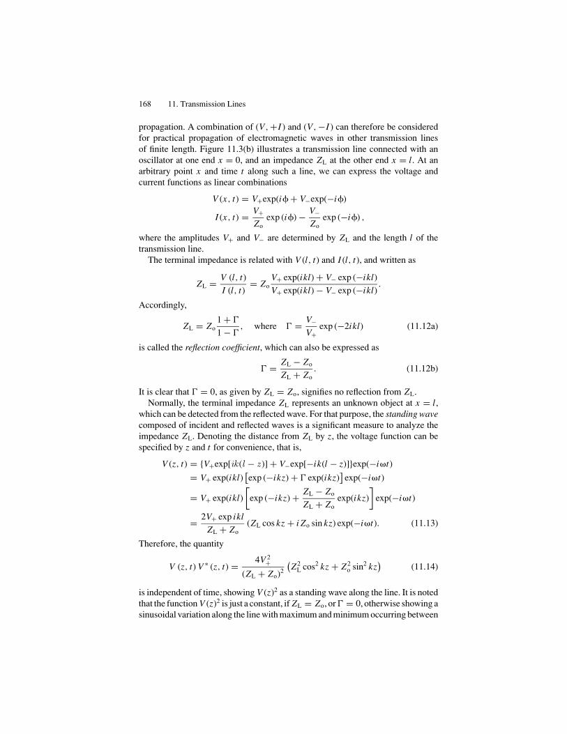
168 11. Transmission Lines
propagation. A combination of (V, +I ) and (V, −I ) can therefore be consideredfor practical propagation of electromagnetic waves in other transmission linesof finite length. Figure 11.3(b) illustrates a transmission line connected with anoscillator at one end x = 0, and an impedance ZL at the other end x = l. At anarbitrary point x and time t along such a line, we can express the voltage andcurrent functions as linear combinations
V (x, t) = V+exp(i� + V−exp(−i�)
I (x, t) = V+Zo
exp (i�) − V−Zo
exp (−i�) ,
where the amplitudes V+ and V− are determined by ZL and the length l of thetransmission line.
The terminal impedance is related with V (l, t) and I (l, t), and written as
ZL = V (l, t)
I (l, t)= Zo
V+ exp(ikl) + V− exp (−ikl)
V+ exp(ikl) − V− exp (−ikl).
Accordingly,
ZL = Zo1 + �
1 − �, where � = V−
V+exp (−2ikl) (11.12a)
is called the reflection coefficient, which can also be expressed as
� = ZL − Zo
ZL + Zo. (11.12b)
It is clear that � = 0, as given by ZL = Zo, signifies no reflection from ZL.Normally, the terminal impedance ZL represents an unknown object at x = l,
which can be detected from the reflected wave. For that purpose, the standing wavecomposed of incident and reflected waves is a significant measure to analyze theimpedance ZL. Denoting the distance from ZL by z, the voltage function can bespecified by z and t for convenience, that is,
V (z, t) = {V+exp[ik (l − z )] + V−exp[−ik(l − z)]}exp(−i�t)
= V+ exp(ikl)[exp (−ikz) + � exp(ikz)
]exp(−i�t)
= V+ exp(ikl)
[exp (−ikz) + ZL − Zo
ZL + Zoexp(ikz)
]exp(−i�t)
= 2V+ exp ikl
ZL + Zo(ZL cos kz + i Zo sin kz) exp(−i�t). (11.13)
Therefore, the quantity
V (z, t) V ∗ (z, t) = 4V 2+
(ZL + Zo)2
(Z2
L cos2 kz + Z2o sin2 kz
)(11.14)
is independent of time, showing V (z)2 as a standing wave along the line. It is notedthat the function V (z)2 is just a constant, if ZL = Zo, or � = 0, otherwise showing asinusoidal variation along the line with maximum and minimum occurring between
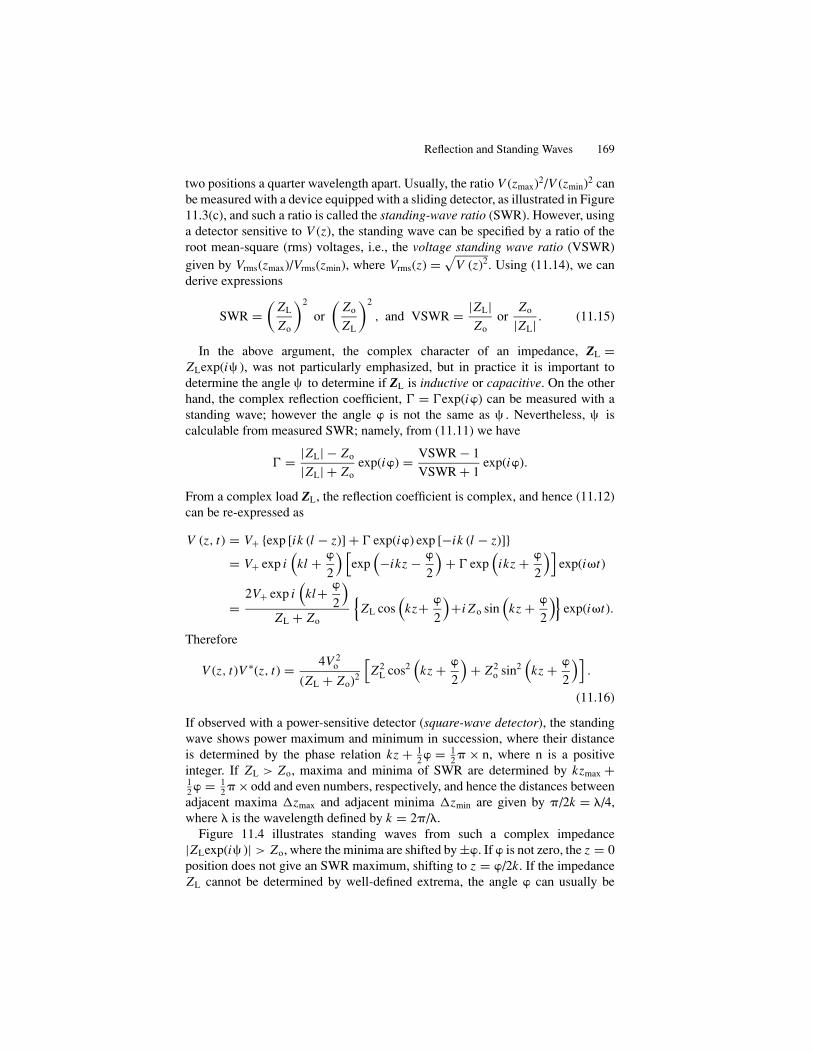
Reflection and Standing Waves 169
two positions a quarter wavelength apart. Usually, the ratio V (zmax)2/V (zmin)2 canbe measured with a device equipped with a sliding detector, as illustrated in Figure11.3(c), and such a ratio is called the standing-wave ratio (SWR). However, usinga detector sensitive to V (z), the standing wave can be specified by a ratio of theroot mean-square (rms) voltages, i.e., the voltage standing wave ratio (VSWR)given by Vrms(zmax)/Vrms(zmin), where Vrms(z) =
√V (z)2. Using (11.14), we can
derive expressions
SWR =(
ZL
Zo
)2
or
(Zo
ZL
)2
, and VSWR = |ZL|Zo
orZo
|ZL| . (11.15)
In the above argument, the complex character of an impedance, ZL =ZLexp(i ), was not particularly emphasized, but in practice it is important todetermine the angle to determine if ZL is inductive or capacitive. On the otherhand, the complex reflection coefficient, � = �exp(i) can be measured with astanding wave; however the angle is not the same as . Nevertheless, iscalculable from measured SWR; namely, from (11.11) we have
� = |ZL| − Zo
|ZL| + Zoexp(i) = VSWR − 1
VSWR + 1exp(i).
From a complex load ZL, the reflection coefficient is complex, and hence (11.12)can be re-expressed as
V (z, t) = V+ {exp [ik (l − z)] + � exp(i) exp [−ik (l − z)]}= V+ exp i
(kl +
2
) [exp
(−ikz −
2
)+ � exp
(ikz +
2
)]exp(i�t)
=2V+ exp i
(kl+
2
)ZL + Zo
{ZL cos
(kz+
2
)+i Zo sin
(kz +
2
)}exp(i�t).
Therefore
V (z, t)V ∗(z, t) = 4V 2o
(ZL + Zo)2
[Z2
L cos2(
kz +
2
)+ Z2
o sin2(
kz +
2
)].
(11.16)
If observed with a power-sensitive detector (square-wave detector), the standingwave shows power maximum and minimum in succession, where their distanceis determined by the phase relation kz + 1
2 = 12 � × n, where n is a positive
integer. If ZL > Zo, maxima and minima of SWR are determined by kzmax +12 = 1
2 � × odd and even numbers, respectively, and hence the distances betweenadjacent maxima �zmax and adjacent minima �zmin are given by �/2k = �/4,where � is the wavelength defined by k = 2�/�.
Figure 11.4 illustrates standing waves from such a complex impedance|ZLexp(i )| > Zo, where the minima are shifted by ±. If is not zero, the z = 0position does not give an SWR maximum, shifting to z = /2k. If the impedanceZL cannot be determined by well-defined extrema, the angle can usually be
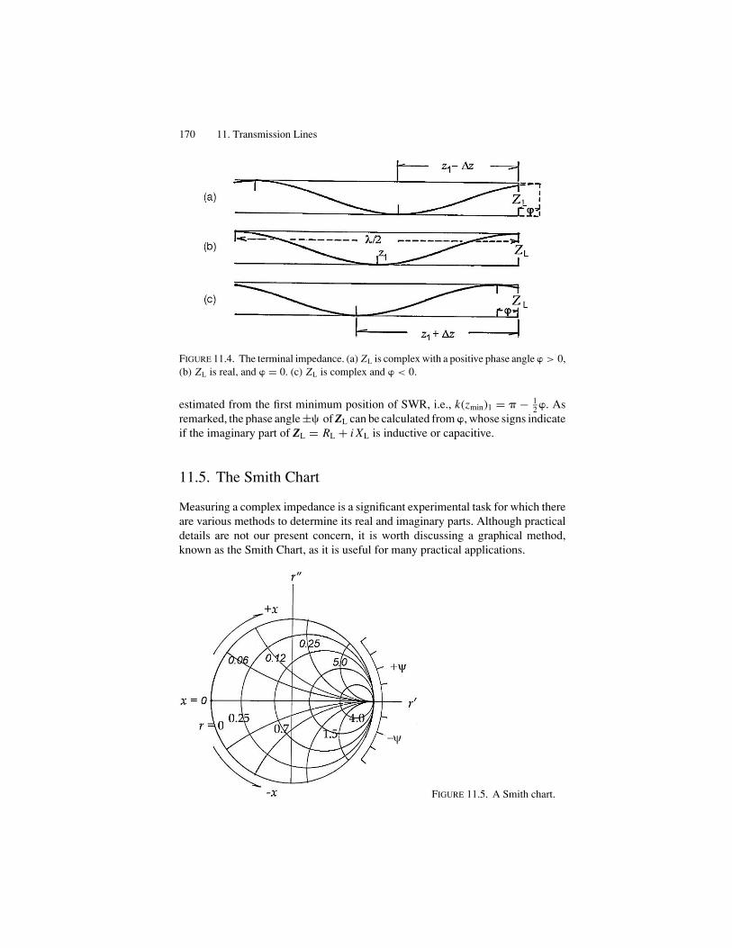
170 11. Transmission Lines
FIGURE 11.4. The terminal impedance. (a) ZL is complex with a positive phase angle > 0,(b) ZL is real, and = 0. (c) ZL is complex and < 0.
estimated from the first minimum position of SWR, i.e., k(zmin)1 = � − 12 . As
remarked, the phase angle ± of ZL can be calculated from , whose signs indicateif the imaginary part of ZL = RL + i XL is inductive or capacitive.
11.5. The Smith Chart
Measuring a complex impedance is a significant experimental task for which thereare various methods to determine its real and imaginary parts. Although practicaldetails are not our present concern, it is worth discussing a graphical method,known as the Smith Chart, as it is useful for many practical applications.
FIGURE 11.5. A Smith chart.

The Smith Chart 171
For convenience, we define the reduced impedance ZL/Zo = z′ + i z′′, and
write � = r ′ + ir ′′. From the relation z′ + i z′′ = 1 + r ′ + ir ′′
1 − r ′ − ir ′′ , we can obtain the
relation (r ′ − z′
1 + z′
)2
+ z′′2 = 1
(1 + z′)2 (i)
and
(r ′ − 1
)2 +(
r ′′ − r ′
z′′
)2
=(
r ′
z′′
)2
. (ii)
For given values of z′ and z′′, (i) and (ii) are both equations of circles in the planeof r ′ and r ′′. Figure 11.5 sketches such families of circles (i) and of (ii) for r ′ = 1,showing a graphical idea of the Smith chart to evaluate the values of z′ and z′′ froma measured impedance. (For details, see “Transmission Line Calculator” by P. H.Smith, Electronics, 12, 29 (1939)).

12The Maxwell Equations
12.1. The Maxwell Equations
Maxwell formulated the laws of electromagnetism by hydrodynamic analogy, bas-ing them on Faraday’s concept of fields. The Maxwell equations constitute funda-mental laws of physics, as recognized in Einstein’s special theory of relativity. Wehave, so far, followed these pioneers’ footsteps in arriving at Maxwell’s equations,the physical implications of which are formally discussed in this chapter.
Except for what is seen in spontaneously magnetized materials, electric chargesat rest and in motion are regarded as the source of electromagnetic fields in matter,including vacuum space, and dynamic electric fields are derived from the timevariation of magnetic fields. On the other hand, the absence of magnetic chargesis accepted as a natural law for the electromagnetic field.
Acting on electric charges and magnetic moments, electric and magnetic fieldvectors E and H are defined as force and torque, respectively, which are tangentialto field-lines, whereas their densities of distribution are signified by another setof vectors, D and B. Although considered as theoretically the same in vacuumspace, the vectors D and E are not necessarily identical in dielectric media, andneither are the vectors B and H in magnetized materials. And, these field vectorsare regarded as originating from charges and currents that are expressed by theirdensities � and j.
The Maxwell theory consists of four differential equations:
(I) j + ∂ D∂t
= curl H, (10.2)
(II) −∂ B∂t
= curl E, (7.5)
(III) div D = � , (4.2c)
(IV) div B = 0. (8.5)
For the field vectors in a vacuum, we have additional relations:
(V.1) D = εo E and B = �o H; (2.7), (7.3)
172

The Maxwell Equations 173
whereas, in dielectric and magnetic media, these are written as
(V.2) D = εo E + P and B = �o H + M, (2.12), (8.23)
where
(V.2) P = � εo E and M = �m�o H, (2.13), (8.22)
representing electric and magnetic properties of matter, respectively. Combiningthese, (V.2) can be expressed as
(V.3) D = εE, ε = (1 + � )εo and B = �H, � = (1 + �m)�o. (2.14a), (8.23)
On the other hand, conducting materials are characterized by the electrical con-ductivity �, for which the Ohm law
(V.4) j = �E,
describes electric properties of normal conductors.In the Maxwell equations, all field vectors are functions of the position r and time
t in the electromagnetic field. In contrast to the densities � and j that are normallyrestricted in limited regions, the field vectors are functions in much broader regionof space. Some regions in the field can be free from � and j, implying that theelectromagnetic field can be extended to a distant point in free space. Hertz (1888)first demonstrated that an electromagnetic signal identified by its frequency travelsa distance through an empty space from one location to another, demonstratingthe presence of a field in a free space.
Figure 12.1(a) sketches Hertz’s experiment, wherein a spark gap attached to aninduction coil generates an intense electromagnetic field, which then propagatesto a “resonance ring” with a spark gap located at a distant point. The ring was
FIGURE 12.1. (a) Hertz’s experiment. (b) A modern version of Hertz’s experiment for prop-
agating electromagnetic waves.
174 12. The Maxwell Equations
designed for its circumference to match the wavelength, where the detected signalis evident from a spark in the gap.
Such an apparatus was primitive by today’s standards, but sufficiently demon-strated a propagating field through an empty space.
The empty space can be characterized by � = 0 and j = 0, in which theMaxwell equations can be written as
curl H = εo
∂ E∂t
, (i)
curl E = −�o
∂ H∂t
, (ii)
div E = 0 (iii)
and
div H = 0. (iv)
Operating “curl” on both sides of (i) and (ii), the operator “curlcurl” can be re-expressed for any arbitrary vector F by using the identity formula as curl curl F ≡grad divF − ∇2 F. Thus, from (i) we obtain
grad divH − ∇2 H = εocurl∂ E∂t
= ∂
∂tcurl E.
Here, from (iv) and (ii) div H = 0 and curl E = −�o
∂ H∂t
, and therefore,
∇2 H − εo�o
∂2 H
∂t2= 0. (12.1a)
Similarly from (ii),
∇2 E − εo�o
∂2 E∂t2
= 0, (12.1b)
where
1√εo�o
= c (12.1c)
is found to be equal to the empirical value of the speed of light in a vacuum.Equations (12.1a) and (12.1b) are wave equations in free space.
The field vectors E and H determined by solutions of these equations are char-acterized as proportional to expi(k · r − �t), representing propagation along thedirection of the wave vector k at the speed c. It is a well-established empirical factthat the electromagnetic field propagates at this speed c, identical to the speed oflight within experimental accuracy, providing solid evidence that optical rays areelectromagnetic waves at shorter wavelengths.

Electromagnetic Energy and the Poynting Theorem 175
All components of E and H in a free space obey the wave equation, indicatingthat in a given direction their space-time variations are basically sinusoidal. Fac-torizing the components into individual functions of space-time, these factors canall be expressed as sinusoidal. Accordingly, it is logical to consider a space-timevariation as described by the phase k . r − �t . Therefore, assuming (E, H) ∝expi(k . r − �t) in (12.1ab), we obtain
c2k2 = �2 and hence ± |k| = �
c,
for the vector k , indicating that the propagation occurs in opposite directions, +kand –k .
12.2. Electromagnetic Energy and the Poynting Theorem
The electromagnetic field should have an energy, as described by the volumedensities 1
2D.E and 1
2B.H in, respectively, the static and stationary fields.
To obtain the expression for energies in a time-dependent field, we calculate
E.∂ D∂t
+ H.∂ B∂t
from (I) and (II); that is,
E.∂ D∂t
+ H.∂ B∂t
= E.curl H − H.curl E − j .E,
which can be written as
∂
∂t
(1
2D.E + 1
2B.H
)= − div (E × H) − j .E.
Considering a volume v enclosed in a surface S = Sn, where n is an outwardnormal, we can define the energy
U =∫
v
u dv, where u = 1
2(D.E + B.H) (12.2)
is the energy density, and hence obtain the expression
∂U
∂t= −
∫v
div (E × H) dv −∫
v
j .Edv = −∮S
(E × H).dS −∫v
j .E dv,
(12.3)
in which the Gauss theorem was applied to convert the first volume integral in thesecond expression to the surface integral in the last one, whereas the j .E termrepresents the heat dissipation in the volume.
Writing
P = E × H (12.4)
which is called the Poynting vector, the integral∮
S P.dS represents an electromag-netic energy flowing out of the volume v per unit time, expressing electromagnetic
176 12. The Maxwell Equations
radiation. With definition (12.4), equation (12.3) can be expressed as
−∂U
∂t=
∮S
P.dS, (12.5)
which is known as the Poynting theorem.
12.3. Vector and Scalar Potentials
The static electric field arising from an electric charge can be described by a
potential function V that satisfies the Laplace-Poisson equation ∇2V = − �
εo
, and
the stationary magnetic field is determined by a vector potential A that is given by∇2 A = −�o j . A time-dependent electromagnetic field due to � and j changingwith time should, therefore, be represented by scalar and vector potentials V andA as combined.
Equation (IV), signifying the absence of magnetic charge, indicates that
B = curl A. (8.9)
Hence, from (II) we have
curl E = −curl
(∂ A∂t
)and curl
(E + ∂ A
∂t
)= 0.
The last equation indicates that the vector E + ∂ A∂t
is given by a gradient of a
scalar function V , that is,
E = −grad V − ∂ A∂t
. (12.6)
Using (12.6) and (8.9) in (III) and (I), we obtain
div(εo E) = −εodiv
(grad V + ∂ A
∂t
)= � , (i)
and
curl
(curl A
�o
)= j + εo
∂
∂t
(−grad V − ∂ A
∂t
). (ii)
Here, in (ii), curl(curl A) ≡ grad(div A) − ∇2 A , and, therefore,
∇2 A − εo�o
∂2 A∂t2
= −�o j + grad
(εo�o
∂V
∂t+ div A
). (12.7a)
As discussed in Section 8.3, the vector potential A cannot be uniquely definedby (8.9), as any other vector
A′ = A + grad � (12.7b)
Retarded Potentials 177
gives B = curl A′ if ∇2� = 0. Also, we note that if we utilize this ambiguity, theequation (12.6) is unchanged with such a redefinition of the scalar potential as
V ′ = V − ∂�
∂t, (12.7c)
as verified by E = −grad V − ∂
∂t
(A′ − grad �
) = −grad V ′ − ∂ A′
∂t. Therefore,
it is always possible to choose a set of (V ′, A′) with a suitable scalar function �atisfying ∇2� = 0, such that
εo�o
∂V
∂t+ div A = 0. (12.7d)
Such a change of (V, A ) with the scalar � stablishes the relation between V and A,and (12.7b) and (12.7c) are referred to as the gauge transformation. The equation(12.7d) unchanged with a gauge transformation is known as the Lorentz condition.
Using (12.7d) in (12.7a), we arrive at an inhomogeneous differential equation
∇2 A − εo�o
∂2 A∂t2
= −�o j . (12.8a)
Equation (i) can also modified by (12.5) and (12.7d) as a form similar to (12.8a), i.e.,
∇2V − εo�o
∂2V
∂t2= − �
εo
. (12.8b)
The equations (12.8ab) are the basic equations to be solved for electromagneticpotentials, when a charge-current distribution is specified. Obviously, at space- andtime coordinates (r , t) far away from � and j , equations (12.8a) and (b) becomehomogeneous wave equations similar to (12.1a) and (b) for E and H in free space.
12.4. Retarded Potentials
In general, we look for the potentials (V, A ) at a given space-time (r , t), whenthe sources (� , j ) are specified as functions of space-time (r ′, t ′). It is significantthat an event at a point r is not detectable at a distant point r ′ at the same time asit occurs at t ′. In other words, it takes certain time for the information to arrive ata point of observation.
We consider that a point charge � at r ′ appears during a short time interval be-tween t ′ and t ′ + �t , and that at a point r no information about � (r ′,t ′) is availableuntil a later time. In this case, the observed charge at a point r at t can be expressedas � (r ′)�(r − r ′)�(t − t ′), where the � are delta functions. Here r − r ′ is the dis-tance, whereas t − t ′ = � represents a period of time after � starts to vary at r ;that is, � is a positive time for � (r ′,t ′) to be detected at r . We define a functionG(r − r ′, t − t ′) to satisfy the equation(
∇2 − 1
c2
∂2
∂� 2
)G(r − r ′, t − t ′) = −�(r − r ′)�(t − t ′). (12.9)

178 12. The Maxwell Equations
If such a function G(r − r ′, � ), namely the Green function, can be obtained, thepotential V (r ) can be calculated as
V (r , t) = − 1
εo
∫ ∫G
(r − r ′, t − t ′)�
(r ′, t ′) d3r ′dt ′. (12.10)
For convenience, if instead of r − r ′ and t − t ′, we write r and � , respectively,the solution of the inhomogeneous equation (12.9) can be expressed by a Fourierexpansion
G(r , � ) = 1
(2)4
∫k-space
d3k
+∞∫−∞
d�� (k, �) exp i(k. r − �� )
and hence
�(r )�(� ) = 1
(2)4
∫k-space
d3k
+∞∫−∞
d� exp i(k. r − �� ).
Therefore, the Fourier transform �(k , �) can be written as
�(k, � ) = 1(�
c
)2
− |k|2,
and hence
G(r , � ) = 1
(2)4
∞∫0
k2 dk
∫0
exp (ik · r ) sin d
2∫0
d�
+∞∫−∞
exp (−i�� )
�2
c2− k2
d�,
where the volume element, i.e., d3k = k2dk sin dd�, is expressed in polar coor-dinates k, , and � with respect to a fixed reference system in the k space.
Here, in the last integral, the integrand has two poles, at � = ±ck on the realaxis in the Re�−Im� plane, assuming � to be a complex variable. Modifying thelast integral as shown below, we can apply the Cauchy theorem to integrate it; thatis,
+∞∫−∞
exp (−i�� )(�
c
)2
− k2
d� = 1
2klim
|�|→∞
∮C
(1
� − ck− 1
� + ck
)exp (−i�� ) d�
= 2i1
2k{exp (−ick� ) − exp (ick� )} = −2
ksin (ck� ) for � > 0,
where C is chosen as a closed path with a large radius |�| to avoid these poles.
Retarded Potentials 179
The integral factor with respect to � is equal to∫ 2
0d� = 2, and the integral
with can be calculated as
+1∫−1
exp (ikr cos ) d (cos ) = 2 sin (kr )
kr, where r = |r |.
Hence, we have
G(r , � ) = − 1
22r
∞∫0
sin (kr ) sin (ck� ) dk, (12.11a)
where the integration should be carried out for positive k over the range 0 ≤ k < ∞,and the integrand can be written as
sin (kr ) sin (ck� ) dk = 14{ exp ik (r − c� ) − exp ik (r + c� )},
ignoring the complex exponentials for −k, because a negative k implies an ad-vanced arrival of information at r , which is physically not acceptable. However,excluding the negative region −∞ < k ≤ 0 from the above calculation is mathe-matically incorrect, and hence we re-write (12.10a) for −∞ < k < +∞ as
G(r , � ) = − 1
82r
+∞∫−∞
exp ik (r − c� ) dk, (12.11b)
after omitting physically incorrect exponentials. Noted that the integral in (12.10b)can be related to the delta-function as
� (r − c� ) = 1
2
+∞∫−∞
exp ik (r − c� ) dk, (12.12)
we obtain
G (r , � ) = − 1
4r�(r − c� ) , (12.13a)
signifying a peak at a later time � = r/c. Returning to original space-time coordi-nates, the Green function can be expressed as
G(r − r ′, t − t ′) = − 1
4∣∣r − r ′∣∣�
{r − r ′ − c
(t − t ′)} . (12.13b)
Using (12.13b) in (12.10), the potential function can be calculated as
V (r , t) = 1
4εo
∫v(r ′)
�(r ′, t ′) �
(r − r ′)
|r − r ′| d3r ′t−|r−r ′|/c∫
−∞�(t − t ′) dt ′,

180 12. The Maxwell Equations
in which
t−|r−r ′|/c∫−∞
�(r ′, t ′) �
(t − t ′) dt ′ = �
(r ′, t −
∣∣r − r ′∣∣c
), (12.14)
expressing the charge density at r ′ at a retarded time t − |r − r ′|/c. Thus, a solutionof the inhomogeneous equation (12.7b) at (r , t) is determined by the charge density(12.13) at a retarded time. Therefore, we can express the scalar potential as
V (r , t) = 1
4εo
∫v(r ′)
�
(r ′, t −
∣∣r − r ′∣∣c
)
∣∣r − r ′∣∣ �(r − r ′) d3r ′. (12.15a)
For a given current density j(r ′, t ′), the inhomogeneous equation (12.8a) can alsobe solved for the vector potential A(r ,t) in a similar manner, resulting in a vectorpotential at a retarded time, i.e.,
A (r , t) = �o
4
∫v(r ′)
j
(r ′, t −
∣∣r − r ′∣∣c
)
∣∣r − r ′∣∣ �(r − r ′) d3r ′. (12.15b)
These potentials (12.15a) and (b) for a retarded time are called the retardedpotentials.
12.5. Multipole Expansion
In practical applications, charges and currents are confined to a finite region ofspace and observed at a distant point away from their distribution. Under such acircumstance, it is significant that the electromagnetic field can approximately bedescribed by a distance r from the center of distribution to the observing pointat a retarded time t − r /c. In addition, the electromagnetic potentials (A, V ) in(12.14a) and (b) are involved in the factor 1/|r − r ′|, which needs to expandedinto a Taylor series, considering r r ′. Here, the retarded time is consideredsufficiently accurate to describe the field at an approximate distance |r − r ′|∼ r ,and we write these source quantities as � (r ′, �R) and j(r ′, �R), where �R = t − r/c.
We apply the Taylor expansion to such a scalar function as F(r ) = jx(r ′, �R
)∣∣r − r ′∣∣ ,
and write
F(r − r ′) = F(r ) − r ′ · gradr F(r ) + · · · ,
in which the terms higher than second order are not particularly necessary becausethey are seldom used in practical applications. Components of the vector potential
Multipole Expansion 181
in (12.15a) can then be expanded in the form
Ax (r , t) = �o
4
∫v(r ′)
(1 − r ′ · gradr + · · ·) jx
(r ′, �R
)r
d3r ′. (12.16)
The vector potential of components given by first term can be expressed as
A1(r , t) = �o
4r
∫v(r ′)
j(r ′, �R
)d3r ′ = �o
4r
∫r ′
dr ′·∮S′
j(r ′, �R
)dS′,
where d3r ′ = dS′ · dr ′, representing a volume element between thin layers ofsurfaces dS′. Using the Gauss theorem, the surface integral can be replaced by− ∫
v(r ′)div j
(r ′, �R
)d3r ′, where the inward direction of j to S′ is considered pos-
itive, which is further modified by the charge-current continuity relation as div
j(r ′, �R) = −∂�(r ′, �R
)∂�R
. Thus, we obtain the expression
A1(r , t) = �o
4r
∂ p(�R)
∂t, where p (�R) =
∫v(r ′)
�(r ′, �R
)r ′d3r ′ (12.17)
represents the electric dipole moment of the source.The second term in expansion (12.16) is
A2x (r , t) = − �o
4
∫v(r ′)
r ′ · gradr
jx(r ′, �R
)r
d3r ′
= − �o
4
[∂
∂x
{1
r
∫v(r ′)
x ′ jx(r ′, �R
)d3r ′
}+ ∂
∂y
{1
r
∫v(r ′)
y′ jx(r ′, �R
)d3r ′
}
+ ∂
∂z
{1
r
∫v(r ′)
z′ jx(r ′, �R
)d3r ′
}].
To make the expression short, we write this with components of r = (xi) andr ′ = (x ′
i ), where i = x, y, and z, and obtain
A2x (r , t) = − �o
4
∑j
∂
∂x j
{1
r
∫v(r ′)
x ′j ji
(r ′, �R
)d3r ′
}, where i = x .
Here, the integrand can be modified as
x ′i ji = 1(x ′
i ji + jjx′i ) + 1(x ′
i ji − jjx′i ),
where the first symmetric part can be further re-written using the relations
∇′.( jx ′i x ′
j ) = j .∇′(x ′i x ′
j ) + (x ′i x ′
j )∇′ j and j .∇′(x ′i x ′
j ) = 1(x ′j ji + jjx
′i ).
182 12. The Maxwell Equations
Using the Gauss theorem,∫v(r ′)
∇′.(
jx ′i x
′j
)d3r ′ =
∮S
x ′i x
′j j .dS = 0,
and the continuity relation,
∇′ j(r ′, �R) = −∂�(r ′, �R
)∂t
,
we arrive at the expression
A2i (r , t) = − �o
8
∑j
∂
∂xj
1
r
[∂
∂t
∫v(r ′)
x ′i x
′j�
(r ′, �R
)d3r ′ +
∫v(r ′)
(x ′
j ji − x ′i jj
)d3r ′
].
(12.18)
Defining the quadrupole tensor as
Qij (�R) =∫r ′
3x ′i x
′j�
(r ′, �R
)d3r ′, (12.19)
the first term of (12.17), representing the quadrupolar contribution to the vectorpotential, can be expressed as
[A2(r , t)]quad =∑
i
ei A2i
(r ′, t
) = − �o
8
∂
∂t
∑ij
ei
∂
∂xj
Qij (�R)
3r.
On the other hand, the second antisymmetric term in (12.17) is written as
[A2(r , t)]mag = − �o
8
∑j
∂
∂xj
∫v(r ′)
x ′j j − jjr ′
rd3r ′ = �o
4∇ × pm(�R)
r,
after a similar manipulation, where the vector pm is defined as
pm(�R) = 1
2
∫v(r ′)
r ′ × j(�R) d3r ′, (12.20)
which is the magnetic moment of the source current. Thus, the electric quadrupoleand magnetic moment represents the charge-current source for the vector potentialin the same order of expansion.
The scalar potential V (r , t) can be expanded in a similar way. Namely,
V (r , t) = 1
4εo
∫v(r ′)
(1 − r ′.gradr + · · ·) �
(r ′, �R
)r
d3r ′,
Multipole Expansion 183
where the first and second terms represent the charge-current source. The first termcan be written as
Vo (r , t) = 1
4εo
q (�R)
r, where q (�R) =
∫v(r ′)
�(r ′, �R
)d3r ′ (12.21)
is the total charge in the source.The second term is
V1 (r , t) = − 1
4εo
gradr
∫v(r ′)
r ′�(r ′, �R
)r
d3r ′ = − 1
4εo
∇rp(�R)
r,
where
p (�R) =∫
v(r ′)
r ′�(r ′, �R
)d3r ′ (12.22)
is the electric dipole moment of the source.It is noted that the dipole moment, magnetic moment, and quadrupole tensor
are all time-dependent, being involved in the time-dependent vector r ′ or its com-ponents, whereas the total charge q(�R) is constant of time. The dipole momentcontributes to both scalar and vector potentials, playing a dominant role for elec-tromagnetic radiation, as discussed in Chapter 13, whereas the total charge is onlysignificant for the Coulomb potential.

13Electromagnetic Radiation
13.1. Dipole Antenna
Hertz demonstrated that electromagnetic radiation could be emitted from a sparkgap in an induction current, thereby giving evidence supporting the Maxwell the-ory. Then, Marconi (1895) invented wireless communication by means of electro-magnetic waves at radio frequencies and opened the modern era of telecommuni-cation technology. Using an antenna, electromagnetic waves can be transmittedthrough open space, and detected by another antenna at a distant location. Al-though not clearly established in Hertz’s experiment, the spark gap played the roleof an antenna for emitting a high-frequency radiation. Further, he demonstrated apersistent oscillation is required for continuous radiation from the antenna.
Figures 13.1(a) and (b) show schematically an antenna attached at the end of atransmission line, where oscillating voltage and current are characterized by thewavelength �, which related to the frequency �, as � = c/�. The figure shows thata sizable standing wave can be set on the antenna if its length is equal to �/2 × anodd integer, depending on the reflecting condition at the input and at the antenna.For short waves the antenna of length �/2, called a half-wave antenna, is mostpractical, serving as an idealized model for dipole radiation. This is discussed inSection 13.2. Also, a loop antenna is in practical use, which is signified by anoscillating magnetic moment for magnetic radiation.
Orbiting electrons in atoms and molecules can also be analyzed for opticalradiations, to which a model similar to an antenna can be applied, supporting theMaxwell theory.
13.2. Electric Dipole Radiation
An oscillating dipole moment defined in (12.17) acts as a source of radiationfrom the antenna in Figures 13.1(a) and (b), where the internal coordinate r ′ ofcharge � (r ′, �R) is considered as varying in sinusoidal motion, corresponding tothe voltage standing wave of �/2. Assuming that the antenna is represented by anoscillating dipole p = po exp(−i�t), it can be observed at a distant point r by the
184
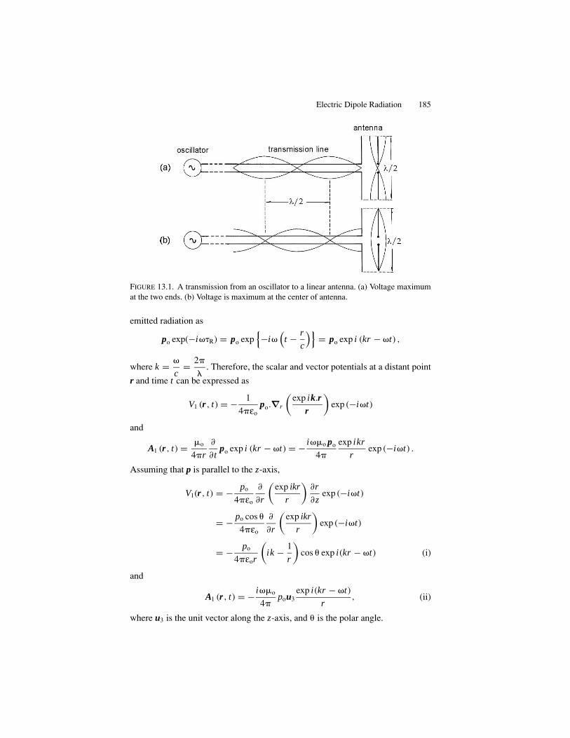
Electric Dipole Radiation 185
FIGURE 13.1. A transmission from an oscillator to a linear antenna. (a) Voltage maximumat the two ends. (b) Voltage is maximum at the center of antenna.
emitted radiation as
po exp(−i��R) = po exp{−i�
(t − r
c
)}= po exp i (kr − �t) ,
where k = �
c= 2�
�. Therefore, the scalar and vector potentials at a distant point
r and time t can be expressed as
V1 (r , t) = − 1
4�εopo.∇r
(exp ik.r
r
)exp (−i�t)
and
A1 (r , t) = �o
4�r
∂
∂tpo exp i (kr − �t) = − i��o po
4�
exp ikr
rexp (−i�t) .
Assuming that p is parallel to the z-axis,
V1(r , t) = − po
4�εo
∂
∂r
(exp ikr
r
)∂r
∂zexp (−i�t)
= − po cos
4�εo
∂
∂r
(exp ikr
r
)exp (−i�t)
= − po
4�εor
(ik − 1
r
)cos exp i(kr − �t) (i)
and
A1 (r , t) = − i��o
4�pou3
exp i(kr − �t)
r, (ii)
where u3 is the unit vector along the z-axis, and is the polar angle.
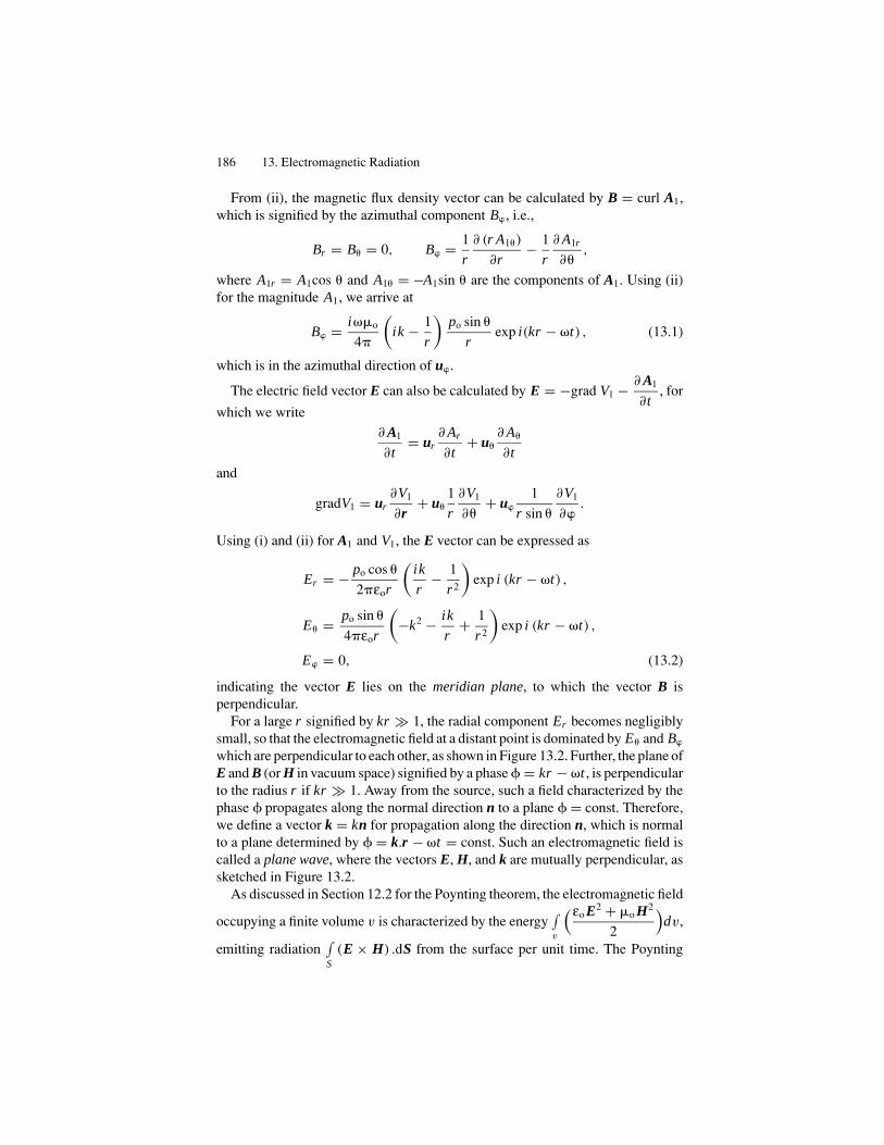
186 13. Electromagnetic Radiation
From (ii), the magnetic flux density vector can be calculated by B = curl A1,which is signified by the azimuthal component B, i.e.,
Br = B = 0, B = 1
r
∂ (r A1)
∂r− 1
r
∂ A1r
∂,
where A1r = A1cos and A1 = −A1sin are the components of A1. Using (ii)for the magnitude A1, we arrive at
B = i��o
4�
(ik − 1
r
)po sin
rexp i(kr − �t) , (13.1)
which is in the azimuthal direction of u.
The electric field vector E can also be calculated by E = −grad V1 − ∂ A1
∂t, for
which we write∂ A1
∂t= ur
∂ Ar
∂t+ u
∂ A
∂t
and
gradV1 = ur∂V1
∂r+ u
1
r
∂V1
∂+ u
1
r sin
∂V1
∂.
Using (i) and (ii) for A1 and V1, the E vector can be expressed as
Er = − po cos
2�εor
(ik
r− 1
r2
)exp i (kr − �t) ,
E = po sin
4�εor
(−k2 − ik
r+ 1
r2
)exp i (kr − �t) ,
E = 0, (13.2)
indicating the vector E lies on the meridian plane, to which the vector B isperpendicular.
For a large r signified by kr � 1, the radial component Er becomes negligiblysmall, so that the electromagnetic field at a distant point is dominated by E and B
which are perpendicular to each other, as shown in Figure 13.2. Further, the plane ofE and B (or H in vacuum space) signified by a phase � = kr − �t , is perpendicularto the radius r if kr � 1. Away from the source, such a field characterized by thephase � propagates along the normal direction n to a plane � = const. Therefore,we define a vector k = kn for propagation along the direction n, which is normalto a plane determined by � = k.r − �t = const. Such an electromagnetic field iscalled a plane wave, where the vectors E, H, and k are mutually perpendicular, assketched in Figure 13.2.
As discussed in Section 12.2 for the Poynting theorem, the electromagnetic field
occupying a finite volume v is characterized by the energy∫v
(εo E2 + �o H2
2
)dv,
emitting radiation∫S
(E × H) .dS from the surface per unit time. The Poynting

Electric Dipole Radiation 187
FIGURE 13.2. Radiation fields from a dipole pat a distant point P .
vector P = E × H represents the radiation, expressing the power for outgoingenergy per unit time. To calculate the radiation from a dipolar source, we considerthe field at kr � 1, or r � �/�, using the definition of wavelength �, where
Er = E0, E = − po sin
4�εork2 exp i�,
and
Br = B = 0, B = −��ok
4�rpo sin exp i�.
Since � = ck and c = 1√εo�o, we can derive that
√εo E = √�o H, and therefore
ur × E =√
�o
εoH. (13.3)
Although field components are conveniently expressed by complex exponen-tials, the observable power should be calculated as a real quantity. We note thattime averages of these complex quantities over the period are given with a factor1
2, so it is convenient to write that
〈P〉t = 1
2Re(E × H∗) = 1
2nRe(E H)
to express the radiation power per unit area. Using the above expressions for E
and H, we obtain
〈P〉t ≈ cp2ok4
32�2εor2sin2 ur , (13.4)
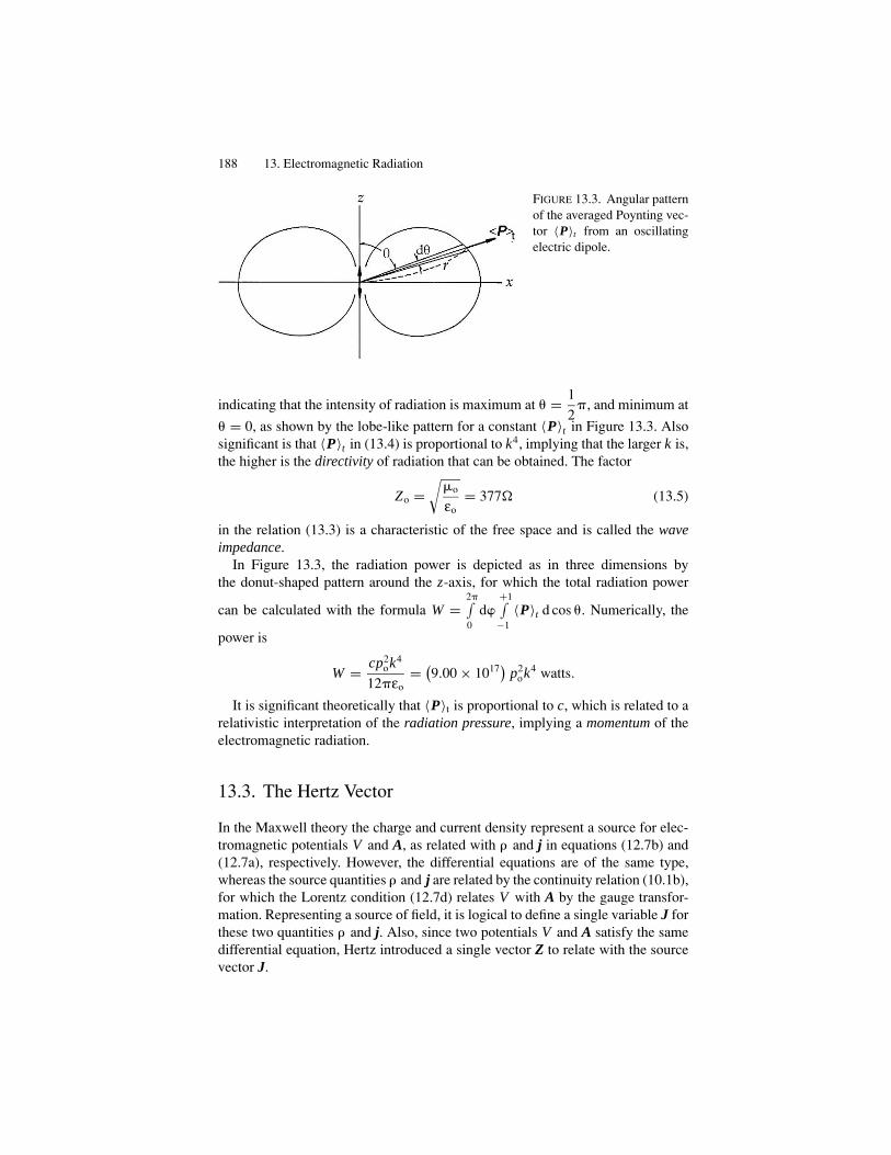
188 13. Electromagnetic Radiation
FIGURE 13.3. Angular patternof the averaged Poynting vec-tor 〈P〉t from an oscillatingelectric dipole.
indicating that the intensity of radiation is maximum at = 1
2�, and minimum at
= 0, as shown by the lobe-like pattern for a constant 〈P〉t in Figure 13.3. Alsosignificant is that 〈P〉t in (13.4) is proportional to k4, implying that the larger k is,the higher is the directivity of radiation that can be obtained. The factor
Zo =√
�o
εo= 377� (13.5)
in the relation (13.3) is a characteristic of the free space and is called the waveimpedance.
In Figure 13.3, the radiation power is depicted as in three dimensions bythe donut-shaped pattern around the z-axis, for which the total radiation power
can be calculated with the formula W =2�∫0
d+1∫−1
〈P〉t d cos . Numerically, the
power is
W = cp2ok4
12�εo= (
9.00 × 10¹⁷) p2ok4 watts.
It is significant theoretically that 〈P〉t is proportional to c, which is related to arelativistic interpretation of the radiation pressure, implying a momentum of theelectromagnetic radiation.
13.3. The Hertz Vector
In the Maxwell theory the charge and current density represent a source for elec-tromagnetic potentials V and A, as related with � and j in equations (12.7b) and(12.7a), respectively. However, the differential equations are of the same type,whereas the source quantities � and j are related by the continuity relation (10.1b),for which the Lorentz condition (12.7d) relates V with A by the gauge transfor-mation. Representing a source of field, it is logical to define a single variable J forthese two quantities � and j. Also, since two potentials V and A satisfy the samedifferential equation, Hertz introduced a single vector Z to relate with the sourcevector J.
The Hertz Vector 189
In (12.7a) and (b), the operator ∇2 − εo�o∂2/∂t2 can be conveniently written
as �2. With this symbol, (12.7a) and (b) can be written as
�2 A = −�o j and �2V = − �
εo, (13.5a)
where
div j + ∂�
∂t= 0 (i)
and
div A + εo�o∂V
∂t= 0. (ii)
Hertz defined a vector Z as
A = �o∂ Z∂t
and V = − 1
εodivZ, (13.6)
which is consistent with the Lorentz condition (ii). On the other hand, the sourcevector J defined as
j = ∂ J
∂tand � = −div J (13.7)
is the same as the continuity relation (i). With these definitions of Z and J, we canwrite the equation
�2 Z = −J, (13.5b)
relating Z, called the Hertz vector, directly to the source J.If the source vector J(r ′, t) is given as
J(r ′, t ′) = p(t ′)�3(r − r ′),
the solution of (13.5b) at a point r can be expressed, as discussed in Section 12.4,as
Z(r , t) = 1
4�
∫v(r ′)
J(r ′, �R
)∣∣r − r ′∣∣ d3r ′, (13.8)
where �R = t −∣∣r − r ′∣∣
cis the retarded time. Expanding
1∣∣r − r ′∣∣ with respect to∣∣∣∣r ′
r
∣∣∣∣ 1 into a Taylor series, the dominant first term is given by
Z1 (r , t) = 1
4�|r − r ′| p(
t − |r − r ′|c
), (13.9)
where
p(�R) = 1
2
∫v(r ′)
r ′ × J(�R) d3r ′
190 13. Electromagnetic Radiation
is referred to as the Hertz dipole. The field vectors B and E can be computed fromthe vector Z as
B = �ocurl
(∂ Z1
∂t
)and E = 1
εograd (div Z1) − �2
o∂2 Z1
∂t2. (13.10)
Example. Field of a Hertz Dipole Parallel to the z-Axis.In this example we discuss the dipole radiation using the Hertz vector, although it
is the same problem as discussed in Section 13.2. Here, we consider the case wherethe source vector J or the corresponding Hertz’s dipole p(�R) is in a fixed directionreferred to as the z-axis. In this case the electromagnetic field of p(�R) can beexpressed by the corresponding Hertz vector Z. In the following only Z1in the firstapproximation is considered, from which the suffix 1 may be omitted for simplicity.Setting a polar coordinate system with respect to the z-axis, components of Z can beexpressed as
Zr = Z cos , Z = −Z sin and Z = 0.
To calculate B and E, we use (13.10), where grad(div Z) and curl Z need to befully expressed by polar coordinates. Abbreviating derivatives of Z as Z ′ = ∂ Z/∂rand Z = ∂ Z/∂t ,
divZ = 1
r2 sin
{∂(r2 sin Zr )
∂r+ 1
r sin
∂ (sin Z)
∂
}= ∂ Zr
∂r= Z ′ cos ,
and therefore
(grad div Z)r = ∂
∂r(Z ′ cos ) = Z
′′cos ,
(grad div Z) = 1
r
∂
∂(Z ′ cos ) = − Z ′
rsin ,
and
(grad divZ) = 0.
On the other hand,
(curl Z)r = 1
r sin
{∂
(sin Z
)∂
− ∂ Z
∂
}= 0,
(curl Z) = 1
r
{1
sin
∂ Zr
∂− ∂(r Z)
∂r
}= 0,
and
(curlZ) = 1
r
{∂(r Z)
∂r− ∂ Zr
∂
}= −Z ′ sin .
Using these results in (13.10), we obtain
Br = 0, B = 0, B = �o Z ′ sin ;
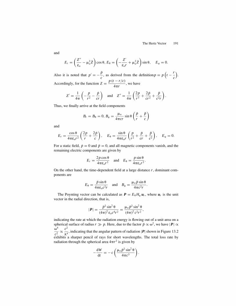
The Hertz Vector 191
and
Er =(
Z ′′
εo− �2
o Z
)cos , E =
(− Z ′
εor+ �2
o Z
)sin , E = 0.
Also it is noted that p′ = − p
c, as derived from the definitionp = p
(t − r
c
).
Accordingly, for the function Z = p (t − r/c)
4�r, we have
Z ′ = 1
4�
(− p
r2− p
cr
)and Z ′′ = 1
4�
(2p
r3+ 2 p
cr2+ p
c2r
).
Thus, we finally arrive at the field components
Br = B = 0, B = �o
4�crsin
(p
r+ p
c
)
and
Er = cos
4�εor2
(2p
r+ 2 p
c
), E = sin
4�εor
(p
r2+ p
cr+ p
c2
), E = 0.
For a static field, p = 0 and p = 0, and all magnetic components vanish, and theremaining electric components are given by
Er = 2p cos
4�εor3and E = p sin
4�εor3.
On the other hand, the time-dependent field at a large distance r , dominant com-ponents are
E = p sin
4�εoc2rand B = �o p sin
4�c2r.
The Poynting vector can be calculated as P = E H ur , where ur is the unitvector in the radial direction, that is,
|P| = p2 sin2
(4�)2 εoc4r2= �o p2 sin2
(4�)2 c2r2,
indicating the rate at which the radiation energy is flowing out of a unit area on aspherical surface of radius r � p. Here, due to the factor p ∝ �2, we have |P| ∝�4
c2∝ c2
�4, indicating that the angular pattern of radiation |P| shown in Figure 13.2
exhibits a sharper pencil of rays for short wavelengths. The total loss rate byradiation through the spherical area 4�r2 is given by
−dW
dt= − c
(�o p2 sin2
4�c3
).
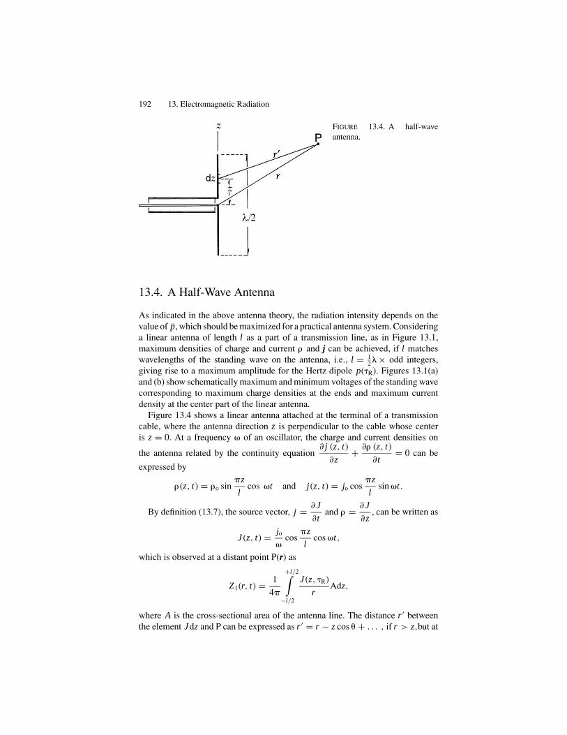
192 13. Electromagnetic Radiation
FIGURE 13.4. A half-waveantenna.
13.4. A Half-Wave Antenna
As indicated in the above antenna theory, the radiation intensity depends on thevalue of p, which should be maximized for a practical antenna system. Consideringa linear antenna of length l as a part of a transmission line, as in Figure 13.1,maximum densities of charge and current � and j can be achieved, if l matcheswavelengths of the standing wave on the antenna, i.e., l = 1
2 � × odd integers,giving rise to a maximum amplitude for the Hertz dipole p(�R). Figures 13.1(a)and (b) show schematically maximum and minimum voltages of the standing wavecorresponding to maximum charge densities at the ends and maximum currentdensity at the center part of the linear antenna.
Figure 13.4 shows a linear antenna attached at the terminal of a transmissioncable, where the antenna direction z is perpendicular to the cable whose centeris z = 0. At a frequency � of an oscillator, the charge and current densities on
the antenna related by the continuity equation∂ j (z, t)
∂z+ ∂� (z, t)
∂t= 0 can be
expressed by
� (z, t) = �o sin�z
lcos �t and j(z, t) = jo cos
�z
lsin �t.
By definition (13.7), the source vector, j = ∂ J
∂tand � = ∂ J
∂z, can be written as
J (z, t) = jo�
cos�z
lcos �t,
which is observed at a distant point P(r) as
Z1(r, t) = 1
4�
+l/2∫−l/2
J (z, �R)
rAdz,
where A is the cross-sectional area of the antenna line. The distance r ′ betweenthe element Jdz and P can be expressed as r ′ = r − z cos + . . . , if r > z,but at

A Loop Antenna 193
a very distant point r � z we may assume r ′ ≈ r . In this case, replacing jo A byIo, Z1(r, t) can be written
Z1(r, t) = Io
4��r
(∫ +l/2
−l/2cos
�z
ldz
)cos ��R = Iol
2�2�rcos ��R,
corresponding to the Hertz dipole p(�R) = 2Iol
��cos ��R, which is given by
2cIo
�2cos ��R for a half-wave antenna l = 1
2 �. The radiation from such an antenna
can be calculated with p(�R), as discussed in the previous section.
13.5. A Loop Antenna
A circular loop antenna, as illustrated in Figure 13.5(a), is also used in practicalapplications. Considering such a circle of radius a in the x, y-plane, an oscillatingcurrent I = Io sin �t on the loop will generate a radiating field. Under a conditionof the wavelength � � a and r � �, the field at a distant point r can be discussedwith the Hertz vector.
Figure 13.4(b) shows the ring current in the x, y-plane, where the current densityelement is given as Iad′ = jAad′ (A is the cross-sectional area of the wire). Thesource current density is then expressed as
jx = − j sin ′, jy = j cos ′ and jz = 0, where j = Io
Asin �t.
The source vector defined by (13.7) can be written as
Jx = J sin ′, Jy= −J cos ′ and Jz = 0, where J = Io
A�cos �t,
with which the Hertz vector can be expressed as
Z (r , t) = 1
4�
∫v(r ′)
J(r ′, �R
)∣∣r − r ′∣∣ d3r ′, where d3r ′ = Aad′.
FIGURE 13.5. (a) A loop antenna. (b) Calculating the radiation from a loop antenna.
194 13. Electromagnetic Radiation
We calculate Z(r, t) approximately as
|r − r ′| = r − a cos �,1∣∣r − r ′∣∣ = 1
r
(1 + a
rcos �
),
where � is the angle between r and r ′ = a, and given by
cos � = sin cos( − ′). (i)
In this case, as the retarded time is given by
�R =(
t − r
c
)+ a
rcos �,
and hence
J = Io
A�cos
{�
(t − r
c
)+ a�
ccos �
}
= Io
A�
{cos
(t − r
c
)− a�
ccos � sin �
(t − r
c
)},
provided that a�/c 1, or a �. Therefore,
Zx = − Ioa
4�r
2�∫0
d′(
1 + a
rcos �
)
×{
cos �(
t − r
c
)− a�
ccos � sin �
(t − r
c
)}sin ′.
Using (i) to replace cos � by sin cos( − ′) and noting that integrals for0 ≤ ′ ≤ 2� will vanish, except for
∫ 2�
0 cos2 ′d′ = ∫ 2�
0 sin2 ′d′ = �, we ob-tain
Zx = − Io�a2 sin
4�crsin �
(t − r
c
)sin ,
and similarly
Z y = Io�a2 sin
4�crsin �
(t − r
c
)cos , and Zz = 0.
Hence,
Z = Io
4�c
�a2 sin
rsin �
(t − r
c
),
and by (13.6)
A = �o Io�a2�
4�c2rsin cos �
(t − r
c
).
The field vectors can be obtained from E = −∂ A∂t
and B = curlA, that is,
E = �o Io�a2�2
4�c2rsin sin �
(t − r
c
)

Plane Waves in Free Space 195
and
H = − 1
�or
∂(r A
)∂r
≈ − Io�a2�2
4�c3rsin sin �
(t − r
c
),
ignoring a term proportional to r−2, which is valid for r � �. In such a distantpoint, we have a simple relation
− E
H= �oc =
√�o
εo,
which is characteristic of a plane wave that is emitted by a magnetic dipole moment,as can be defined by
pm(r ′, t) = Io�a2 sin �t.
In this case, we notice that E and H vectors are perpendicular, though they are outof phase, exhibiting phase difference �. The time average of the Poynting vectorcan be expressed as
〈Pr 〉t = − �oc
(4�)2
( pm
c
)2 (�
c
)4 sin2
r2,
and the total radiation power is
dW
dt= −
2�∫0
d
+1∫−1
〈P〉t r2d (cos ) = −�oc
4�
(2
3c4p2
m�4
).
13.6. Plane Waves in Free Space
In free space away from the source, the Maxwell equations are specified locallyby � = 0 and j = 0. We have shown in Section 12.1 that the field vectors E andH in free space are derived from the wave equation, i.e.,(
∇2 − 1
c2
∂2
∂t2
)(E, H) = 0, (13.11)
where c = 1/√εo�o is equal to the speed of light. It has been confirmed that light
speed is identical to that of electromagnetic propagation at lower frequencies.Hence, (13.11) is believed to govern all electromagnetic waves, including opticallight. Solutions of (13.11) express propagating waves from a remote source sig-nified by oscillating charges at a specific frequency �, which are expressed by asinusoidal function of x and t .
As related to the dipolar source J(r′, t ′) that is observed as J(
r, t −∣∣r − r ′∣∣
c
),
phases of the field vectors E and H are expressed as �(
t − r
c
)+ �, where r =
|r − r ′|, and � depends on the nature of the distant source. Complicated radiationfields near the source may be considered as trivial at distant points for a periodic

196 13. Electromagnetic Radiation
FIGURE 13.6. Plane waves. (a) A wavefront of a plane wave. (b) An example of plane waves(E, H) that are in phase.
repetition of E and H, where we can only be concerned about the periodic variationin space-time r and t or in the phase �t– k.r , where |k| = �/c, with respect to areference near the observing point. Yet, the phase difference between E and H, thatis 0 or �s is significant for a source: It is either an electric or a magnetic dipole,respectively. The solution of (13.11) can be expressed by sin or cos functions witharbitrary phases, however it is more convenient to treat them as complex functionsof a phase, considering that only the function’s real part is physically meaningful.With the ratio �/c = k, called the wave number, we can write
E = Eo exp i(kr − �t) and H = Ho exp i(kr − �t + ), (13.12)
where Eo and Ho are amplitude vectors, and Eo ⊥ Ho, as verified in Sections 13.3and 13.4, at a large distance r . Figure 13.2 illustrates such vectors E, H and k at adistant point (r , , ).
Further, E and H are constant at all points on a plane of kr − �t = const. Hence,k can be considered as a vector k parallel to the normal n of such a plane, i.e., k= kn, which is called the wave vector. Define an arbitrary point on the plane by thevector r, the algebraic equation of the plane is expressed by � = k.r − �t+ const,on which lie field vectors E and H. Taking two such parallel planes where�� = 2� the perpendicular distance is given by � = 2�/k, which is referredto as the wavelength. For such a plane wave we have relations
� = ck, k = 2�/�, �� = 2�c. (13.13)
Figure 13.6(a) shows a plane with respect to the laboratory system X, Y , andZ . We indicated the direction of propagation along the z direction, and the planeis determined by E and H, whose directions are designated by the x and y axes,as shown in Figure 13.6(b). In the figure, plane waves in phase are illustrated.
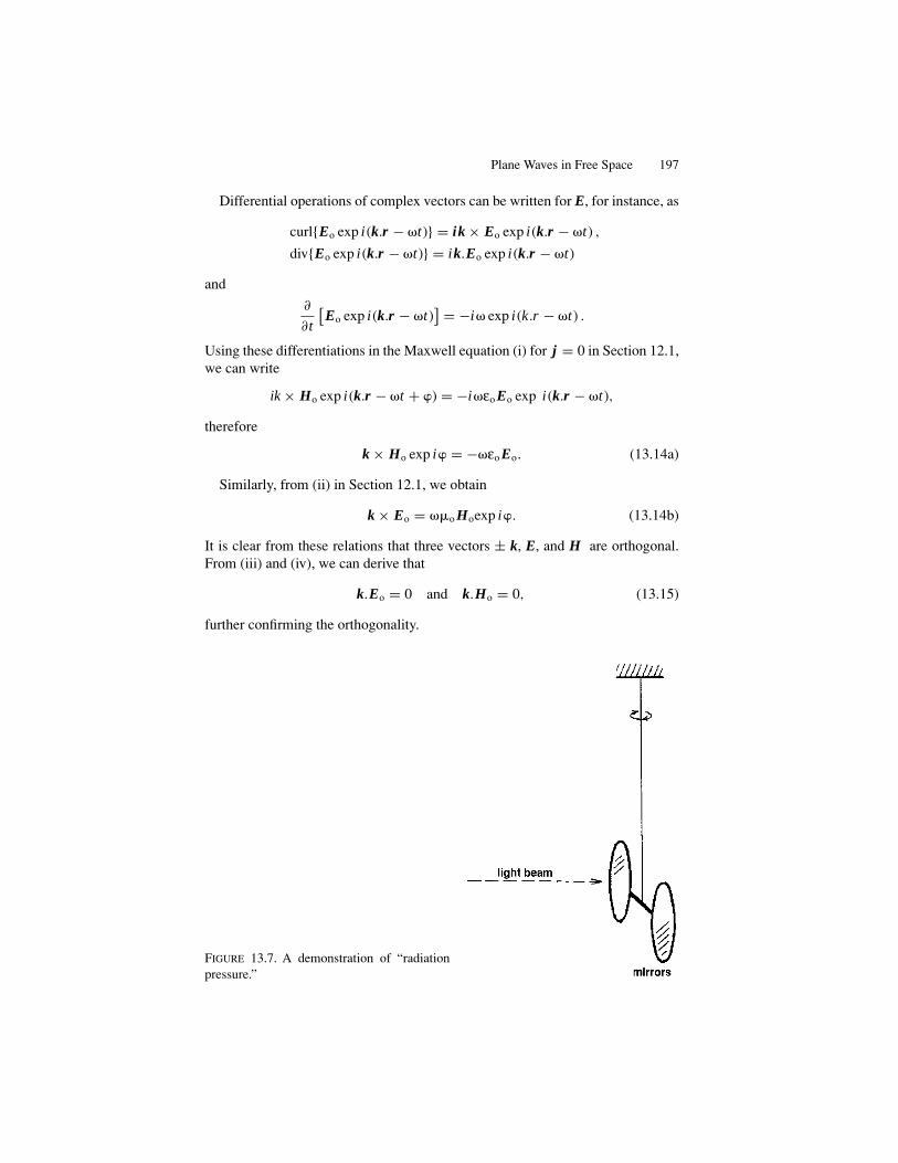
Plane Waves in Free Space 197
Differential operations of complex vectors can be written for E, for instance, as
curl{Eo exp i(k.r − �t)} = ik × Eo exp i(k.r − �t) ,
div{Eo exp i(k.r − �t)} = ik.Eo exp i(k.r − �t)
and
∂
∂t
[Eo exp i(k.r − �t)
] = −i� exp i(k.r − �t) .
Using these differentiations in the Maxwell equation (i) for j = 0 in Section 12.1,we can write
ik × Ho exp i(k.r − �t + ) = −i�εo Eo exp i(k.r − �t),
therefore
k × Ho exp i = −�εo Eo. (13.14a)
Similarly, from (ii) in Section 12.1, we obtain
k × Eo = ��o Hoexp i. (13.14b)
It is clear from these relations that three vectors ± k, E, and H are orthogonal.From (iii) and (iv), we can derive that
k.Eo = 0 and k.Ho = 0, (13.15)
further confirming the orthogonality.
FIGURE 13.7. A demonstration of “radiationpressure.”

198 13. Electromagnetic Radiation
The plane wave is characterized by its phase � = k.r − �t = const, which isnothing but the algebraic equation of a plane kx x + ky y + kzz = −�(t) + const,where the components of the wavevector k are proportional to the direction cosinesof the normal n. As discussed already,
Zo = |Eo||Ho exp i| =
√�o
εo= 377.6 �,
which is the wave impedance in free space.The energy density of plane electromagnetic waves is evaluated as
u(r ) = εo
2Eo.E∗
o + �o
2Ho.H∗
o = εo E2o,
with which the energy in a given volume is expressed as U = ∫v
u (r ) d3r . Accord-
ing to the Poynting theorem, −dU
dt=
∫S
(E × H).dS, indicating that electromag-
netic field energy in the volume v is decreased as a function of time. Applyingthe theorem to plane waves propagating at a constant wavevector k, the Poyntingvector can be calculated as
E × H∗ = E2o
��ok = c2u (r )
�kn = cu (r ) n.
On the other hand,dU
dtcan be interpreted mechanically as the power Fc, where F
is effectively a force exerting on the surface S, we can write the relation Fc = cuSn .Therefore we can regard the quantity P = F/Sn = u as the radiation pressure.
Writing F = dp
dtto define the momentum of the field confined to v, we obtain
the energy-momentum relation as U = cp, that is consistent with the relativisticequation for a zero-mass particle. Substantiated by a simple experiment illustratedin Figure 13.7, the mechanical properties of a plane wave are expressed quantum-theoretically by photons characterized by energy U = nh� and momentump = nh�/c, where n is the number of photons.

14The Special Theory of Relativity
14.1. Newton’s Laws of Mechanics
In Newton’s mechanics, a particle of mass m in motion under a force F is describedby the equation
md2rdt2
= F. (i)
The mass m and the force F represent, respectively, the mechanical property of aparticle and the cause of motion, quantities whose values are independent of theobserver, whereas the acceleration d2r/dt2 describes the motion of a particle withrespect to the observer. On the other hand, the equation of motion is unchanged bya velocity transformation, i.e., dr/dt = dr′/dt + vv, between two observers, wherevv is a constant relative speed, implying that r(t) and r′(t) in different referencesare identical. In this context, Newton’s law of motion is invariant for independentobservers moving with a constant relative speed, whereas the time tremains as auniversal variable for these observers. Therefore, a particle at absolute rest cannotbe identified in such a framework of space-time of Newton’s mechanics.
Considering two reference systems S(x , y, z) and S′(x ′, y′, z′) moving at aconstant relative velocity v along the x and x ′ directions assumed to be parallel,equation (i) is unchanged under a transformation
x ′ = x − vt, y′ = y, z′ = z and t ′ = t, (14.1a)
which is referred to as the Galilean transformation, and for which we have thevelocity relation
V ′ = V − v. (14.1b)
In contrast, the laws of electromagnetism are not invariant under the Galileantransformation because the Maxwell equations involve both static and movingcharges. These equations are signified by the speed of light c that is constant for allobservers, which contradicts (14.1b). On the other hand, Maxwell’s equations areverified as invariant under a coordinate transformation called the Lorentz trans-formation, as will be discussed later. Nevertheless, the Galilean transformation
199

200 14. The Special Theory of Relativity
(14.1a) is consistent with the Lorentz transformation in the limit of c → ∞. In histheory of relativity, Einstein proposed that all physics laws—including the lawsof electromagnetism—must be invariant under the Lorentz transformation. New-ton’s law is regarded as approximately invariant, as can be verified in the limit ofc = ∞.
Faraday and Maxwell considered that the electromagnetic field represents aphysical object that occupies a volume in space encompassing an empty space andmaterials as well. Electromagnetically, the vacuum can be regarded as a mediumcharacterized by constants εo and �o, in which the speed of light is given byc = 1
√εo�o. It was once thought that the whole universe was filled with a hypo-thetical material called ether through which electromagnetic waves were assumedto propagate. In this postulate absolute rest would be attributable to ether; this no-tion was, however, proved incorrect by the Michelson–Morley experiment (1887),which provided convincing evidence against the ether theory.
14.2. The Michelson–Morley Experiment
Michelson and Morley carried out an optical experiment to determine if “ether”really existed or not; they obtained a negative result for the ether hypothesis.Figure 14.1 shows their experimental layout, which consisted of a large turntableon which their optical apparatus was installed.
If light travels at the speed c with respect to ether that was considered as abso-lutely at rest, light should travel at a speed c + v for a moving observer at a speed v,according to (14.1b). These authors considered that v could be the speed of rotating
FIGURE 14.1. The Michelson—Morley experiment.

The Michelson–Morley Experiment 201
Earth, on which their laboratory is steadily located. The turntable was utilized toset the light beam in the direction of Earth’s rotation, where monochromatic lightfrom a steady source on the table was split by a semi-transparent mirror A towardmirrors 1 and 2, located in parallel and perpendicular directions to Earth’s rotation,respectively. Reflected light beams from 1 and 2 were viewed by the scope B inthe figure. Although not shown in the figure, another glass plate similar to A wasinstalled in the experiment to adjust the path length.
Adjusting the light path from A to the mirror 1 in parallel with the directionof the rotating Earth, the light propagated toward the mirror at the speed c + v,whereas the light reflected from the mirror 1 propagated backward at the speedc − v. Denoting the distance between A and the mirror 1 by l1, the time t1 for thereturn trip A → mirror 1 → A is given by
t1 = l1
c + v+ l1
c − v= 2cl1
c2 − v2
On the other hand, on the path from A to the mirror 2, the light propagated at thespeed
√c2 − v2. Therefore, letting the distance be l2, the time t2 for the return trip
A → mirror 2 → A can be expressed as
t2 = 2l2√c2 − v2
.
Accordingly, returning back to A from mirrors 1 and 2 by reflection, the two lightbeams have a time difference
�t = t2 − t1 = 2
c
(l2√
1 − v2
c2
− l1
1 − v2
c2
).
Next, the whole apparatus was rotated by 90◦ so that the light from A to mirror 2was parallel to v; the other beam from A to mirror 1 was perpendicular to v. Whenthe two beams returned back to A, the time difference �t ′ can be written as
�t ′ = 2
c
( −l1√1 − v2
c2
+ l1
1 − v2
c2
).
If �t �= �t ′ in these experiments, an interference pattern should be observed at B,due to a small but detectable phase difference, which can be expressed as
�(�t − �t ′) ≈ �v2 (l1 + l2)
c3,
assumingv c. In the apparatus, typically l1 = l2 =1.2 m,v = 3 × 10⁴ m/sec and2�/� = 2 × 10⁻¹⁵ sec. If the ether theory were correct, Michelson and Morleyexpected to observe a shift of 0.04 fringe at a time interval of �t ′ − �t = 8 ×10⁻¹⁷ s with a visible light, which, in their experiment, was a detectable order ofmagnitude. Yet, no fringe shift was detected within optical accuracy, thus providing
202 14. The Special Theory of Relativity
evidence that refuted the ether theory. Accordingly, the speed of light must beconsidered to be exactly the same in all inertial systems.
On the basis of the Michelson–Morley experiment, Lorentz and Fitzgerald pro-posed that the length of a moving object measured by a stationary observer appearscontracted by a factor
√1 − v2/c2, whereas its length perpendicular to the mov-
ing direction remains unchanged. Although proposed before Einstein’s discovery,their hypothesis was proven to be a direct consequence of the relativity theory.Such an effect on length of a moving object is known as the Lorentz–Fitzgeraldcontraction.
14.3. The Lorentz Transformation
In Newton’s mechanics, time is considered an absolute measure for any eventin progress, and hence a variable independent from an observer. In the relativitytheory, on the other hand, it is a variable between observers in relative motion.
A “clock” set in a system S indicates a time t for an event in progress. However,for the same event observed in a different system S′ moving at a relative speedv, the time t ′ is not necessarily the same as t measured in S. The reason is thatinformation transmitted by means of the light signal takes finite time to reachthe observer. Therefore, it is significant to realize that no event can be observed“simultaneously” by different observers.
In this context, there is no absolute time; clocks can be set to one time when theirindividual systems coincide, but they show different times if they are in motionrelative to each other. With an individual time set in each system, we use fourcoordinates, x , y, z, and t , in the reference system S to describe a physical eventprogressing in space-time. On the other hand, as confirmed in the Michelson–Morley experiment, a light signal propagates at a constant speed c in any systemS moving at a constant relative speed v with respect to another system S′.
Observed in two systems S and S′ in relative motion at a speed v, we consideran event described as (�x , �t) and (�x ′, �t ′), respectively. For a light signalpropagates in all directions in space at the speed c, the frontal spheres are givenby
(�x)2 + (�y)2 + (�z)2 = c2(�t)2 and (�x ′)2 + (�y′)2 + (�z′)2 = c2(�t ′)2
(14.1)
in S and S′, respectively. However, assuming parallel motion of S and S′ in theirrespective x and x ′ directions, we may consider�y = �z = 0 and�y′ = �z′ = 0,for which (14.1) can be simplified as
�x = c�t and �x ′ = c�t ′. (14.2)
On the other hand, for such S and S′ the Galilean formula (14.1a) should bemodified by introducing factors � and � ′, as
�x ′ = � (�x − v�t) and �x = � ′(�x ′ + v�t ′); (14.3)
The Lorentz Transformation 203
however, we should have � = � ′ in order for the Newton equation (i) to be invari-ant. Using (14.2) in these equations, we can obtain the relation between the timeintervals �t and �t ′, i.e.,
c�t ′ = � (c�t − v�t) and c�t = � ′(c�t ′ + v�t ′).
Therefore,
� 2 = 1
1 − v2
c2
.
Writing � = v
c, the transformation formula can be elaborated from (14.2) and
(14.3), resulting in
�x ′ = �x − v�t√1 − �2
, �y′ = �y, �z′ = �z and �t ′ =�t − v�x
c2√1 − �2
,
(14.4a)
and the inverse relations
�x = �x ′ + v�t ′√1 − �2
, �y = �y′, �z = �z′ and �t =�t ′ + v�x ′
c2√1 − �2
,
(14.4b)
which are collectively known as the Lorentz transformation.We note that (14.4a) can be reduced to
�x ′ = �x − v�t, �y′ = �y, �z′ = �z and �t ′ = �t,
if � c or v c, which are identical to (14.1a). Therefore, Newton’s law canbe regarded as a valid approximation for v c, a condition that is valid for mostterrestrial phenomena. For example, the speed of the Earth orbiting around theSun is about 30 km/s, and hence � = 1.000000005 ≈ 1, so for this Newton’sequation is sufficiently accurate, whereas for such fast-moving particles as muonsin cosmic rays, � = 0.98, for which the relativistic effects are very significant.It is clear from the definition of � that the speed v cannot exceed the speed oflight c, which is considered the fastest speed in the universe. In the special theoryof relativity, Einstein proposed that all physical laws must be invariant under theLorentz transformation. Here, by “special” he meant that invariant laws are heldin all systems of observation moving at constant relative speed, which is generallycalled the inertial system.
Emitted from a point x , y, z at a time t in an inertial system S, a light sig-nal propagates spherically in all directions in space at speed c. Including t asan additional coordinate with x , y, z, a set of four coordinates x , y, z, t canspecify such a physical event in four-dimensional space, and we write x1 = x ,x2 = y, x3 = z and x4 = ict, for convenience, where i = √−1. An inertial system

204 14. The Special Theory of Relativity
in four dimensions can therefore be characterized by the invariance of the metricdefined as
|�s|2 =∑
i�x2
i = �x2 + �y2 + �z2 − c2�t2,
where �s is a four-dimensional distance vector with components �x , �y, �z,and ic�t in the system S. In fact, for an accelerating system Einstein elaboratedthe general theory of relativity; the metric invariance is violated in an acceler-ating system, thus representing a distorted four-dimensional space. Supported byextraterrestrial evidence, his general theory plays an important role in astrophysics.
For a particular event stationary in S′, i.e., �x ′ = �y′ = �z′ = 0, the timeinterval �t ′ is Lorentz invariant because |�s|2 is invariant. Hence, this �t ′ = �is referred to as a proper time interval in S′, indicating the timescale of a clockattached to S′. On the other hand, for an event at a fixed time in S′, i.e., �t ′ = 0, thecorresponding �x ′ represents (if �y′ = �z′ = 0) a proper length lo of an objectattached to S′. Therefore, in a system S moving at a relative speed v, such eventscan be observed as
�t = �� and lo = ��x
from (14.3), assuming v < c. Hence, writing these as
�t = �√1 − �2
> � and �x = lo
√1 − �2 < lo (14.5)
which are known as the Lorentz dilatation and the Lorentz contraction, respectively.Such relativistic relations are substantial in many high-speed phenomena, wherev is close to c. For example, a muon particle has life of the order of 2 × 10⁻⁶ s,which can be considered as the proper time � in the system S′ moving with cosmicray. Therefore, as observed in the system S on the ground, the distance for a muonto travel between the moments of creation and disintegration can be estimated byc�t = c�� ∼ 6 × 10² m if its speed is considered close to c. The second relationin (14.5) is exactly Lorentz–Fitzgerald’s hypothesis proposed for the Michelson–Morley experiment.
14.4. Velocity and Acceleration in Four-Dimensional Space
In this section we discuss transformations of velocity and acceleration componentsbetween inertial systems. We assume that S and S′ are in parallel, and v is in thedirection of the x and x ′ axes. In this case, the coordinate transformation is writtenas
�x1 = �(�x ′
1 + v�t ′) , �x2 = �x ′2, �x3 = �x ′
3,
�t = �( v
c2�x ′
1 + �t ′)
.

Velocity and Acceleration in Four-Dimensional Space 205
Three-dimensional components u1, u2, u3 of the four-dimensional velocity can bedefined as
u1 = lim�t→0
�x1
�t= lim
�t→0
�x ′1
�t ′ + v
1 + v
c2
�x ′1
�t ′
= u′1 + v
�(
1 + v
c2u′
1
) ,
u2 = u′2
�(
1 + v
c2u′
1
) , and u3 = u′3
�(
1 + v
c2u′
1
) ,
and the relation between �t and �t ′ can be expressed as
�t = �t ′(
1 + v
c2u′
1
).
The temporal advance of a stationary event in an inertial system can be describedby the proper time � , which is, however, measured as �� by an observer in a systemmoving at a relative speed v. Therefore, for a given system of reference, we canlogically define a speed, dx1/d� for an object, referring to the proper time � . Fromthe general relation �t = �� , we have dt /d� = � . So, writing a position vector inthe four-dimensional space as a row matrix
〈r | = (x1, x2, x3, x4) = (x, y, z, ict),
the four-dimensional velocity can be expressed as
〈v| = (v1, v2, v3, v4),
where
v1 = dx1
d�= dx1
dt
dt
d�= �u1,
v2 = dx2
d�= �u2, v3 = dx3
d�= �u3,
and
v4 = dx4
d�= d (ict)
d�= ic�.
in the system S′. Here, a so-called bra vector 〈r | is defined to facilitate matrixmultiplication with the corresponding ket vector as a column matrix, i.e.
〈r | =
⎛⎜⎜⎝
r1
r2
r3
r4
⎞⎟⎟⎠ .
Because the proper time is Lorentz invariant, the velocity vector 〈v| is transformedas 〈r |, that is,
v1 = �
(v ′
1 − iv
cv ′
4
), v2 = v ′
2, v3 = v ′3 and v4 = �
(iv
cv ′
1 + v ′4
).
206 14. The Special Theory of Relativity
Similarly, the four-dimensional acceleration can be defined as
〈a| = d 〈v|d�
,
which transforms similarly to the velocity 〈vvv|. It is, however, neither simple noruseful for practical applications for us to elaborate the derivation here. Neverthe-less, we can derive the following relation
〈v | v〉 =4∑
i=1
v 2i = � 2v2 − � 2c2 = − c2,
and hence
d
d�〈v | v〉 = 2 〈v | a〉 = 0, (14.6)
which is a useful relation.
14.5. Relativistic Equation of Motion
Newton’s law is fundamental in all inertial systems and sufficiently accurate, pro-vided that a system’s relative speed v is sufficiently small compared with the speedof light c. Under this condition , the equation of motion is regarded as invariantunder the Lorentz transformation.
Newton’s equation of motion for a particle of mass mo in the three-dimensionalspace is
F = mo
dudt
,
and the corresponding equation in four-dimensional space-time can be written as
〈F| = mo
d 〈v|d�
,
where the four-dimensional vector 〈F| = (F1, F2, F3, F4) are defined by
(F1, F2, F3) = mo�d
(v1, v2, v3
)dt
= � F,
implying that the effective mass m = mo� is not a constant and is written as
m = mo√1 − �2
. (14.7)
For the fourth component F4 we use the relation (14.7), which can be written as
v1F1 + v2F2 + v3F3 + v4F4 = 0,
and hence
� 2u · F + ic�F4 = 0,
Relativistic Equation of Motion 207
from which we obtain
F4 = i�
cu.F.
Here, writing that u.F = dKdt , the quantity K is the kinetic energy, for which we
have the relation
dK
dt= c
i�F4 = c
i�mo�
dv4
dt= d
(moc2�
)dt
because of v4 = ic� integrating this equation we obtain
K = moc2√1 − �2
+ Ko = mc2 + Ko, (14.8)
where Ko is constant. Expanding 1/√
1 − �2 for a small �, i.e., v c, (14.8) canbe written as
K − Ko = �K = mc2 = moc2 + 1
2mov
2 + · · · (14.9a)
For a particle of v = 0, m = mo, which is therefore called the rest mass. In thiscase we have the relation
�K = moc2, (14.9b)
signifying the equivalence of mass and energy, which is substantiated by a massdefect of an atomic nucleus. The nucleus of an atom of atomic number Z andmass number A is composed of Z protons and (A − Z ) neutrons, but the nuclearmass m is empirically given by
m = Zmp + (A − Z )mn − �,
where � is interpreted as related to the energy released when these protons andneutrons are bound to form nuclear matter. Hence, the mass defect � is a usefulmeasure for the binding energy �c2 of a nucleus. According to (14.9a), besidesthe mass energy moc2, �K represents the classical kinetic energy 1
2mov
2 in thelimit of v → c.
The relativistic momentum in four-dimensional space can be defined as
〈p| = mo 〈v| = (p1, p2, p3, p4),
where
p1 = mo�u1, p2 = mo�u2, p3 = mo�u3, p4 = imoc� = i�K
c.
We can see that
〈p | p〉 =4∑
i=1
p2i = p2
1 + p22 + p2
3 − �K 2
c2= mo 〈v | v〉 = m2
oc2,

208 14. The Special Theory of Relativity
which is constant and Lorentz invariant. Also, the result indicates that
�K 2 = c2 p.p + m2oc4 where p = mu = �K
c2u. (14.10)
We considered a particle of a finite rest mass mo in the above argument. Onthe other hand, to travel at the speed c, a particle should have zero mass mo = 0,for which �K = cp from (14.10). It is noted that an electromagnetic radiationis characterized by a pressure described by the relation U = cp, as discussed inthe previous chapter. Therefore, such a pressure p should be originated from theintrinsic nature of the electromagnetic field, unrelated to the gravitational character,which may therefore be expressed effectively by mo = 0. To be consistent withsuch a relativistic argument, the electromagnetic radiation can be considered asconsisting of a number of massless particles whose momentum is p = �K /c.
14.6. The Electromagnetic Field in Four-Dimensional Space
Maxwell’s equations constitute the fundamental law for electromagnetism in allinertial systems, which should therefore be invariant under the Lorentz transforma-tion. Physically, the charge and current density are conserved as a source, obeyingthe equation of continuity. It is fundamental that such a conservation law shouldgovern Maxwell’s equations under the Lorentz transformation. Writing the conti-nuity equation in two systems S and S′ as
∂�
∂t+ div (�vvv) = 0 and
∂� ′
∂t ′ + div(� ′v′) = 0,
the variables (� , �v) and (� ′, � ′v ′) can be transformed in four dimensions similarto a four velocity vector (v, ic). We can therefore define the four-dimensional vector
〈s| = (�v1, �v2, �v3, ic� ),
thereby expressing the continuity relation as
∑i
∂si
∂xi
= 0 and∑
i
∂s ′i
∂x ′i
= 0. (14.11)
These si and s ′i are linearly related, so that
s ′i = iksk,
for which the product 〈s| s〉 should be invariant. Namely, we have∑i
sisi =∑
i
s ′is
′i ,
hence
�2(v21 + v2
2 + v23 − c2) = constant.

The Electromagnetic Field in Four-Dimensional Space 209
Expressing this constant as � 2o and writing � = ��o, we obtain
〈s| = �o 〈v| , (14.12)
resulting in the linear relation between the four charge-current density vector andthe four velocities, as expected.
The electric field vector E in three-dimensional space exerts a force F = qEon a charge q . The force in four-dimensional space can be written as 〈F| =(�qE1, �qE2, �qE3, iq�
c vvv.E), for which the four-dimensional velocity is 〈v| =(�v1, �v2, �v3, ic� ). In this context, the electric field in four-dimensional spacecan be defined as a 4 × 4 tensor that relates 〈F| with 〈v|. Therefore, expressingsuch a tensor by E, we have the expression
〈F| = q
c〈v| E. (14.13)
On the other hand, writing
〈F| = q
c(ic� ) (−i E1) ,
q
c(ic� ) (−i E2) ,
q
c(ic� ) (−i E3) ,
q
ci�u.E,
the tensor E can be given explicitly as
E =
⎛⎜⎜⎝
0 0 0 −i E1
0 0 0 −i E2
0 0 0 −i E3
i E1 i E2 i E3 0
⎞⎟⎟⎠ , (14.14)
which is asymmetric with respect to the indexes, i.e., Eij = −Eji.The Lorentz transformation between four-dimensional vectors 〈r | = (x, y,
z, ict) and
⟨r ′∣∣ =
⎛⎜⎜⎝
x ′
y′
z′
ict ′
⎞⎟⎟⎠
can be expressed as
T =
⎛⎜⎜⎝
� 0 0 −iv�/
c0 1 0 00 0 1 0
iv�/
c 0 0 �
⎞⎟⎟⎠ , (14.15)
for which we have the relation T−1T = e, where e the unit matrix in four dimen-sions, thereby transforming force 〈F| as
〈F’ | = 〈F | T−1 and |F’ 〉 = T |F 〉 .
Using (14.13), the latter can be expressed as
|F’ 〉 = q
cTE |v 〉 = q
cTET−1 |v’ 〉 ,

210 14. The Special Theory of Relativity
and therefore the electric field tensor (14.12) in the S′ system is transformed to S′
as
E′ = TET−1. (14.16)
Calculating the detail with (14.13),
E′ =
⎛⎜⎜⎝
� 0 0 iv�/
c0 1 0 00 0 1 0
−iv�/
c 0 0 �
⎞⎟⎟⎠ ×
⎛⎜⎜⎝
0 0 0 −i E1
0 0 0 −i E2
0 0 0 −i E3
i E1 i E2 i E3 0
⎞⎟⎟⎠
×
⎛⎜⎜⎝
� 0 0 −iv�/
c0 1 0 00 0 1 0
iv�/
c 0 0 �
⎞⎟⎟⎠ .
=
⎛⎜⎜⎝
0 −v� E2
/c −v� E3 −i E1
v� E2
/c 0 0 −i� E2
v� E3
/c 0 0 −i� E3
i E1 i� E2 i� E3 0
⎞⎟⎟⎠ .
Changing notation as
E ′1 = E1, E ′
2 = � E2, E ′3 = � E3; B ′
2 = −v� E3
c2, B ′
3 = v� E2
c2,
we can write that
E′ =
⎛⎜⎜⎝
0 cB ′3 −cB ′
2 −i E ′1
−cB ′3 0 0 −i E ′
2
cB ′2 0 0 −i E ′
3
i E ′1 i E ′
2 i E ′3 0
⎞⎟⎟⎠ . (14.17)
Accordingly,
∣∣F′⟩ = q
cE′ |v〉 = q�
⎛⎜⎜⎝
u′2 B ′
3 − u′3 B ′
2 + E ′1
−u′1 B ′
3 + E ′2
u′1 B ′
2 + E ′3
iu′ · E′/c
⎞⎟⎟⎠ ,
which can be interpreted in three-dimensional space in S′ system as
F′ = F′1i + F′
2 j + F′3k
�= q
(E′ + u′ × B′) ,
where
E′ = E ′1i + E ′
2 j + E ′3k and B′ = B ′
2 j + B ′3k
are conventional expressions in three dimensions, and where the vector B′ shouldbe the magnetic field observed in S′ that is transformed from the electric field in S.
Thus, the tensor E′ is not purely electric, indicating that an electric field in amoving system S′ also consists of a magnetic feature, as observed in S. Needless

The Electromagnetic Field in Four-Dimensional Space 211
to say, this is equivalent to considering that a moving charge at a velocity v in amagnetic field B will be deflected by the dynamic electric field given by v × B.
In four-dimensional space-time, the electromagnetic field (E, B) is thereforeconsidered as a 4 × 4 tensor in a form generalized from (14.17) in S′, that is
G =
⎛⎜⎜⎝
0 cB3 −cB2 −i E1
−cB3 0 cB1 −i E2
cB2 −cB1 0 −i E3
i E1 i E2 i E3 0
⎞⎟⎟⎠ , (14.18)
which is anti-symmetrical, i.e., Gij = −Gji, being composed of
(G23, G31, G12) = cB and (G11, G22, G33) = E. (14.19)
Calculating the transformed G′ = T−1GT from the elements G′ij we obtain
E ′1 = E1, E ′
2 = � (E2 − vB3) , E ′3 = � (E3 + vB2)
B ′1 = B1, B ′
2 = �(
B2 + v
c2E3
), B ′
3 = �(
B3 − v
c2E2
).
Solving these for components in the S system,
E1 = E ′1, E2 = �
(E ′
2 + v3 B ′3
), E3 = �
(E ′
3 − vB ′2
)B1 = B ′
1, B2 = �(
B ′2 − v
c2E ′
3
), B3 = �
(B ′
3 + v
c2E ′
2
),
which can also obtained by exchanging the primed and unprimed components, e.g.,E1 and E ′
1, B2 and B ′2, etc., and replacing v by – v in the former set. Considering
v = (v, 0, 0), from the latter set we can show that
E = � E′ + (1 − � )vvv
(vvv.E′)v2
+ �(vvv × B′)
B = � B′ + (1 − � )vvv
(vvv.B′)v2
+ � (vvv × E′),
which are a valid form by the Lorentz transformation between S and S′.The Maxwell equations are composed by first derivatives of field vectors with
respect to space-time coordinates. Therefore, such derivatives should be trans-formed as a four-vector matrix in the four-dimensional space-time. We notice thatderivatives of the field tensor like ∂Gij
/∂xk should be combined to construct a
four-vector tensor. Calculating4∑
i=1
∂Gij
∂xi
for j = 1, 2, 3, 4 with (14.17), we obtain
4∑i=1
∂Gi1
∂xi
= ∂G11
∂x1
+ ∂G21
∂x2
+ ∂G31
∂x3
+ ∂G41
∂x4
= −c∂ B3
∂x2
+ c∂ B2
∂x3
+ i∂ E1
∂x4
= −c�o (curl H)1 + i
icεo
∂ D1
∂t,
212 14. The Special Theory of Relativity
which can be expressed as
= �oc
{− (curl H)1 + ∂ D1
∂t
}.
Similarly,
4∑i=1
∂Gi2
∂xi
= �oc
{− (curl H)2 + ∂ D2
∂t
},
4∑i=1
∂Gi3
∂xi
= �oc
{− (curl H)3 + ∂ D3
∂t
}
and
4∑i=1
∂Gi4
∂xi
= i (div E) .
Hence, these derivatives constitute a four-vector that can be written as(4∑
i=1
∂Gi1
∂xi
,
4∑i=1
∂Gi2
∂xi
,
4∑i=1
∂Gi3
∂xi
,
4∑i=1
∂Gi4
∂xi
)∝ �o |v 〉 , (14.20)
corresponding to the Maxwell equations
curl H − ∂ D∂t
= j and div D = � . (i)
The field tensor G per se is clearly insufficient for all of the Maxwell equationsin space-time. The other Maxwell equations,
curl E + ∂ B∂t
= 0 and div B = 0, (ii)
can formally be obtained from (i) by substituting (H, D) by (E, − B), replacing theelectrical source by a zero magnetic source, i.e., ( j, � ) → (0, 0). In this context,instead of G defined by (14.18) we consider another field tensor G∗ that is obtainedby replacing (B, E) by (E, −B), that is
G∗ =
⎛⎜⎜⎝
0 −i E3 i E2 cB1
i E3 0 −i E1 cB2
−i E2 i E1 0 cB3
−cB1 −cB2 −cB3 0
⎞⎟⎟⎠ , (14.21)
which is known as the dual of the tensor G.By similar calculation on the dual G∗, we can show that
4∑i=1
∂G∗ik
∂xi
= −i (curl E)k − i∂ Bk
∂t, where k = 1, 2, 3

The Electromagnetic Field in Four-Dimensional Space 213
and
4∑i=1
∂G∗i4
∂xi
= −c div B.
Therefore, we have a four-vector(4∑
i=1
∂G∗i1
∂xi
,
4∑i=1
∂G∗i2
∂xi
,
4∑i=1
∂G∗i3
∂xi
,
4∑i=1
∂G∗i4
∂xi
)= 0, (14.22)
which is consistent with the Maxwell equations (ii).Although the mathematical detail for the tensor G and its dual G∗ and their
transformation was not discussed, the Lorentz invariance of the Maxwell theorywas verified in the above argument. Those readers interested in the formal analysisshould refer to books on the relativity theory, such as The Theory of Relativity byC. Møller.
16Guided Waves
16.1. Propagation Between Parallel Conducting Plates
Wave equations have a simple plane-wave solution that can be obtained in freespace and used for a field bounded by rectangular boundaries. In such cases,as a consequence of the linear differential equations involved, solutions canbe expressed by a Fourier series of sinusoidal functions of the phase variable� = k.r − �t . Normally, a light beam propagates as a free wave but is coupledwith a reflected wave at a boundary point, as discussed in the previous section.Nevertheless, such a reflection in optics is a significant concept for general elec-tromagnetic waves in open and bound space. For electromagnetic applications theradiation needs to be guided in a desired direction, where it is necessary to specifydirections of the propagating and reflecting power of the wave from a target object.In this chapter we discuss the basic principle for such guided waves in moderncommunication and guidance.
For the purpose of illustration we consider two parallel conducting plates of alarge area, where plane electromagnetic waves can pass through the space, reflect-ing back and forth between the plates, as shown in Figure 16.1. Plane waves aretransmitted zigzag in the x direction, a situation for which we consider two specificcases, namely, those where the E and H vectors are polarized in perpendicular tothe z direction, respectively, as in Figure 16.1(a) and (b). The k vector changesthe direction in the xz-plane of incidence at every reflection in a manner similarto a single reflection. Such polarized waves are referred to as being in transverseelectric (TE) and transverse magnetic (TM) modes, for E and H, respectively;both are transversal to the x-axis.
Denoting the two conductors as plates 1 and 2, reflections of a propagating wavecan be described by the wavevector k that changes the direction zigzag in the planeS between 1 and 2. Such reflections take place at any phase � = k.r − �t + 2�m,where m is an integer, and therefore we can apply the same boundary condition atevery phase separated by 2�. At each point of reflection on the plates 1 and 2, wecan write incident and reflected waves, referring to the E vector, as
Ei(1) = Eio exp[i(ki1.r − �t)], Er(1) = Ero exp[i(kr1.r − �t)],
226
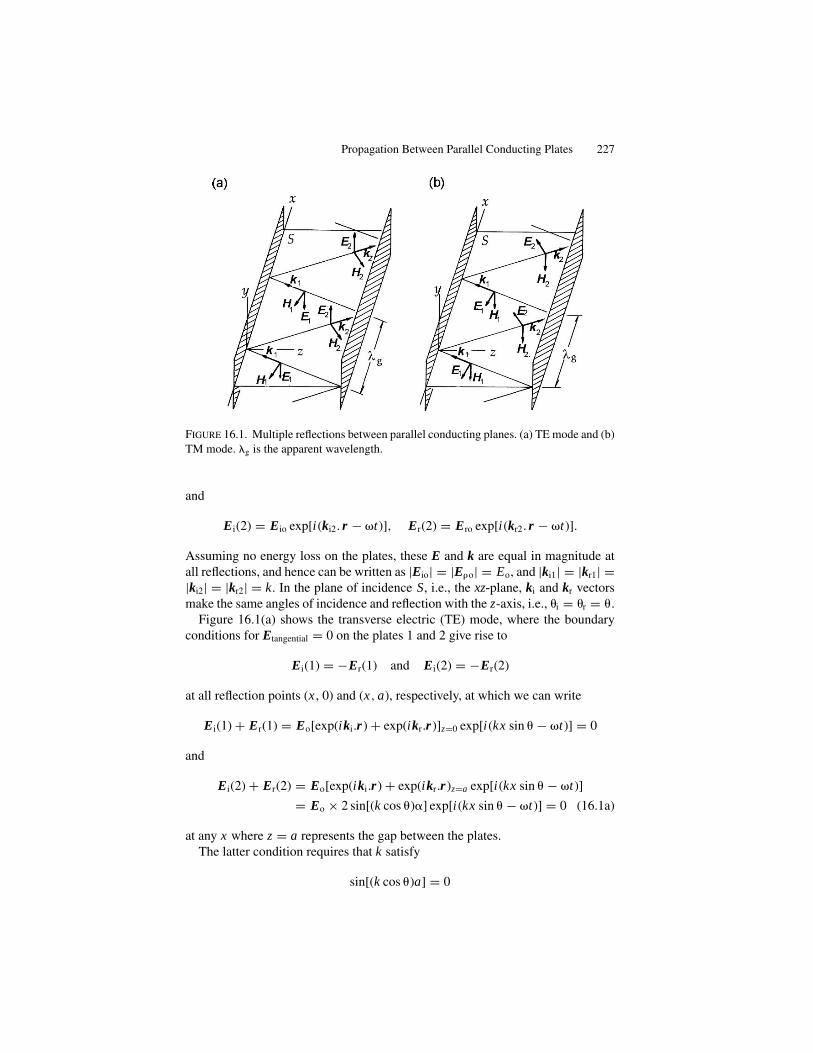
Propagation Between Parallel Conducting Plates 227
FIGURE 16.1. Multiple reflections between parallel conducting planes. (a) TE mode and (b)
TM mode. �g is the apparent wavelength.
and
Ei(2) = Eio exp[i(ki2. r − �t)], Er(2) = Ero exp[i(kr2. r − �t)].
Assuming no energy loss on the plates, these E and k are equal in magnitude atall reflections, and hence can be written as |Eio| = |E�o| = Eo, and |ki1| = |kr1| =|ki2| = |kr2| = k. In the plane of incidence S, i.e., the xz-plane, ki and kr vectorsmake the same angles of incidence and reflection with the z-axis, i.e., �i = �r = �.
Figure 16.1(a) shows the transverse electric (TE) mode, where the boundaryconditions for Etangential = 0 on the plates 1 and 2 give rise to
Ei(1) = −Er(1) and Ei(2) = −Er(2)
at all reflection points (x , 0) and (x, a), respectively, at which we can write
Ei(1) + Er(1) = Eo[exp(iki.r ) + exp(ikr.r )]z=0 exp[i(kx sin � − �t)] = 0
and
Ei(2) + Er(2) = Eo[exp(iki.r ) + exp(ikr.r )z=a exp[i(kx sin � − �t)]
= Eo × 2 sin[(k cos �)�] exp[i(kx sin � − �t)] = 0 (16.1a)
at any x where z = a represents the gap between the plates.The latter condition requires that k satisfy
sin[(k cos �)a] = 0

228 16. Guided Waves
at an arbitrary x , signifying (k cos�)a = m�, where m is any integer. Using thewavelength defined by � = 2�/k, we obtain
� = 2a
mcos � = �c cos �, (16.1b)
which should be shorter than �c = 2a/m for such a wave to propagate throughbetween the plates. If � > �c, the angle � in (16.1b) cannot be obtained; sucha wave cannot go through. The parameter �c is called the cut-off wavelength,signifying that the gap a between the plates limits the propagation by � < �c. Theindex m specifies various modes of TE waves, among which the mode m = 1 issignified by the longest cut-off wavelength �c = 2a.
The corresponding H vectors in the TE mode are all in the plane S, as shown inFigure 16.1(a). Using similar notation as we did for the E vectors, at every pointof reflection the H vectors are expressed as
Hi(1) = [−iHo cos � − kHo sin �] exp(−i�t),
Hr(1) = [−iHo cos � + kHo sin �] exp(−i�t),
and
Hi(2) = [−iHo cos � + kHo sin �] exp[i(kx sin � + ka cos � − �t)],
Hr(2) = [−iHo cos � − kHo sin �] exp[i(kx sin � − ka cos � − �t)].
Accordingly, at a point (x , 0)
Hi(2) + Hr(2) = −i[2Ho cos � cos(ka cos �)] exp[i(kx sin � − �t)] = 0 (16.2)
because of (16.1b). It is noted from (16.1a) and (16.2) that both tangential compo-nents of E and H should vanish periodically at xm, so that kxmsin� − kxm−1sin� =2�. In this context, xm − xm−1 = �g is an apparent wavelength for propagationalong the x direction, namely,
�g = �
sin �. (16.3)
For a practical waveguide, �g is also known as the guide wavelength, serving as asignificant measure for a standing wave. By definition, �c and �g are related, i.e.,
1
�2= 1
�2c
+ 1
�2g
. (16.4)
Figure 16.1(b) shows a transverse magnetic (TM) mode for which a calculationsimilar to TE mode can be carried out. In this case,
H(1) = Hi(1) + Hr(1) = 0 and H(2) = Hi(2) + Hr(2) = 0
on the plates 1 and 2. Hence, the H and E vectors at (x , 0, a) near a reflection point(x , 0, a) can be written as
H(x) = jEo
Zo
cos (ka cos �) exp [i (kx sin � − �t)]

Uniform Waveguides 229
and
E(x) = −i[2i Eo cos � sin(ka cos �)] exp[i(kx sin � − �t)]
−k[2Eo sin � cos(ka cos �)] exp[i(kx sin � − �t)].
Therefore, from the boundary condition for the H(x) we obtain cos(ka cos�) = 0,leading to the cut-off wavelength �c = 4a/m for TM mode. On the other hand, thephase factor is the same as in TE mode, so that the apparent wavelength is givenby �g = �/ sin �.
16.2. Uniform Waveguides
Referring to the coordinate axes in Figure 16.1, the electromagnetic fields betweenparallel conducting plates are independent of the y-axis in both TE and TM modes.We can therefore place a conducting plate at any place in parallel with the xz-plane, thereby leaving the field-lines unchanged. In fact, such polarized waves canpropagate through a rectangular tube of a cross-sectional area a × b as long as thewavelength is shorter than the cut-off wavelength determined by 2a. Such a tubingof uniform cross-sectional area is in use for modern high-frequency circuitry and isknown as a waveguide. For practical applications, rectangular and circular tubingis common, although theoretically the shape of the cross-section may be arbitrary,provided that it is uniformly made.
16.2.1. Transversal Modes of Propagation(TE and TM Modes)
We set a rectangular coordinate system where the x-axis represents the axis ofa waveguide, and the transversal area is described by y and z coordinates. Thepropagating fields can then be expressed as
E = Et + Ex i and H = Ht + Hx i, (16.5)
where (Ex , Hx ) and (Et, Ht) are called longitudinal and transversal components.We can show that these longitudinal components cannot be simultaneously zeroand the propagating wave is characterized by either one of these unvarnished Ex ,Hx , i.e., Hx = 0 or Ex = 0. These modes are referred to, respectively, as the TE andTM modes. In a coaxial cable, in contrast, there exists such a propagating wavecharacterized by both vanishing longitudinal components called the transversalelectric-magnetic (TEM) mode, being analogous to a plane wave in free space.
For such guided waves, boundaries at both ends have to be specified by theirrespective connecting devices: e.g., for an isolated long waveguide the boundariesare considered open at x = ±∞, whereas in infinite parallel plates, the boundariesare closed (or short-circuited) at z = ±∞, but open at x = ±∞. We can show thatsuch a TEM mode cannot occur in a waveguide with a cross-section of a single
230 16. Guided Waves
boundary, whereas this transmission is possible in a waveguide with two closedboundaries.
Equations (16.5) indicate that the field vectors can be factorized into productsof separate functions of (y, z, t) and (x , t). Hence,
Et = (Ey, Ez) and Ht = (Hy, Hz),
and all the field components are expressed to have a factor exp[i(kx x − i�t)].The basic equations div E = 0 and div H = 0 can be written as
∂ Ey
∂y+ ∂ Ez
∂z+ ikx Ex = 0 (ia)
and
∂ Hy
∂y+ ∂ Hz
∂z+ ikx Hx = 0. (ib)
On the other hand, equations curl E = i�oH and curl H = −i�εoE are expressed,respectively, as
∂ Ez
∂y− ∂ Ey
∂z= i�o Hx , (iia)
ikx Ez − ∂ Ex
∂z= i�o Hy, (iib)
and
∂ Ex
∂y− ikx Ey = i�o Hz ; (iic)
and
∂ Hz
∂y− ∂ Hy
∂z= −i�εo Ex , (iiia)
ikx Hz − ∂ Hx
∂z= −i�εo Ey, (iiib)
and
∂ Hx
∂y− ikx Hy = −i�εo Ez . (iiic)
Combining (iib) and (iiic), we can derive the relation between Ey and Hz , whileEz and Hy can be related using (iic) and (iiib). Namely,
Ey = − i
kc2
(�o
∂ Hx
∂z− kx
∂ Ex
∂y
), (iva)
Ez = − i
kc2
(�o
∂ Hx
∂y+ kx
∂ Ex
∂z
)(ivb)
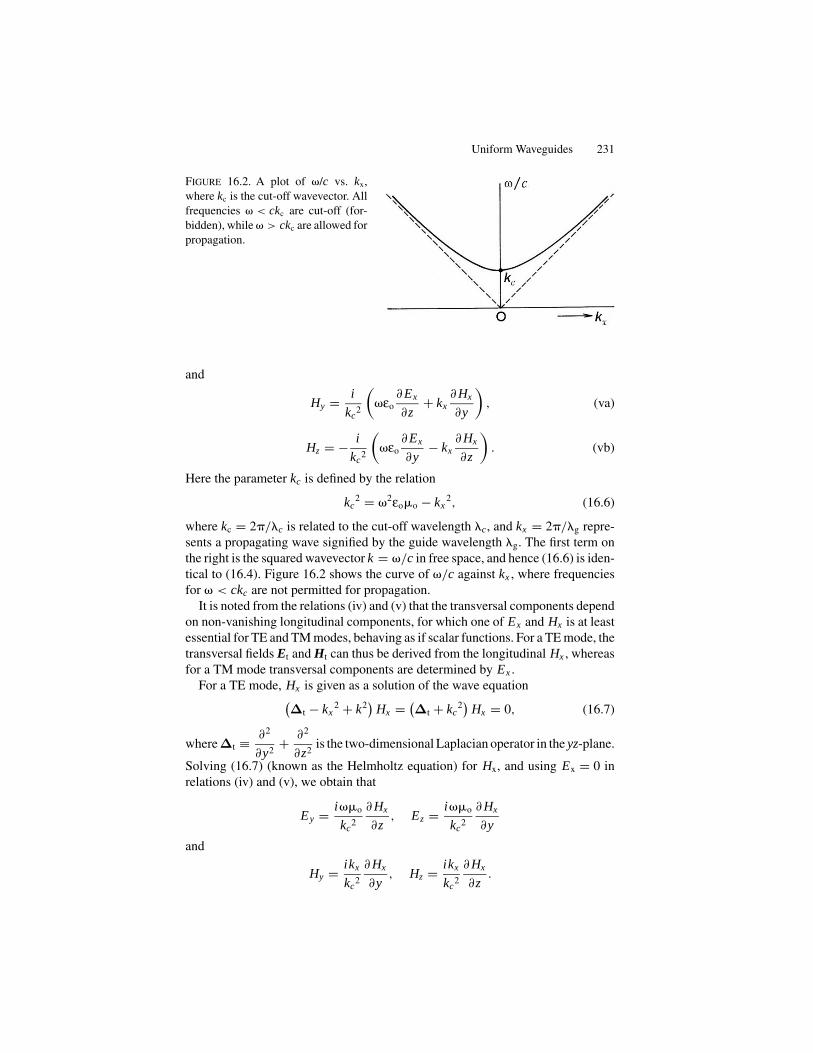
Uniform Waveguides 231
FIGURE 16.2. A plot of �/c vs. kx,
where kc is the cut-off wavevector. All
frequencies � < ckc are cut-off (for-
bidden), while � > ckc are allowed for
propagation.
and
Hy = i
kc2
(�εo
∂ Ex
∂z+ kx
∂ Hx
∂y
), (va)
Hz = − i
kc2
(�εo
∂ Ex
∂y− kx
∂ Hx
∂z
). (vb)
Here the parameter kc is defined by the relation
kc2 = �2εoo − kx
2, (16.6)
where kc = 2�/�c is related to the cut-off wavelength �c, and kx = 2�/�g repre-sents a propagating wave signified by the guide wavelength �g. The first term onthe right is the squared wavevector k = �/c in free space, and hence (16.6) is iden-tical to (16.4). Figure 16.2 shows the curve of �/c against kx , where frequenciesfor � < ckc are not permitted for propagation.
It is noted from the relations (iv) and (v) that the transversal components dependon non-vanishing longitudinal components, for which one of Ex and Hx is at leastessential for TE and TM modes, behaving as if scalar functions. For a TE mode, thetransversal fields Et and Ht can thus be derived from the longitudinal Hx , whereasfor a TM mode transversal components are determined by Ex .
For a TE mode, Hx is given as a solution of the wave equation(Δt − kx
2 + k2)
Hx = (Δt + kc
2)
Hx = 0, (16.7)
whereΔt ≡ ∂2
∂y2+ ∂2
∂z2is the two-dimensional Laplacian operator in the yz-plane.
Solving (16.7) (known as the Helmholtz equation) for Hx, and using Ex = 0 inrelations (iv) and (v), we obtain that
Ey = i�o
kc2
∂ Hx
∂z, Ez = i�o
kc2
∂ Hx
∂y
and
Hy = ikx
kc2
∂ Hx
∂y, Hz = ikx
kc2
∂ Hx
∂z.
232 16. Guided Waves
These results can be written with vector notation as
Ht = ikx
kc2
gradt Hx and Et = − ik Zo
kc2
[i × gradt Hx
],
where Zo =√
o
/εo is the wave impedance, as previously defined in (13.6), and
the component Hx is regarded as a scalar function. These transversal fields arerelated by
Et = −k Zo
kx[i × Ht] and Ht = kx
k Zo
[i × Et] (16.8)
in the TE mode, where the H vector is not transversal, as given by H = Ht + Hx i.For the TM mode where Hx = 0, we can obtain the following expressions after
a similar calculation to the TE mode:(Δt − kc
2)
Ex = 0, (16.9)
Et = ikx
kc2
gradt Ex , Ht = ik
Zokc2
[i × gradt Ex
],
and
Et = −kx Zo
k[i × Ht] (16.10)
16.2.2. Transversal Electric-Magnetic Modes (TEM)
In free space the E and H vectors of a propagating wave are both transversal andperpendicular to the wavevector k. For a guided wave such a TEM mode can alsobe transversal, depending on the boundaries. Since both axial components Ex andHx are zero in TEM mode, the equations (ia), (ib), (iia), and (iiia) can be written as
∂ Ey
∂y+ ∂ Ex
∂x= 0,
∂ Hy
∂y+ ∂ Hz
∂z= 0
and
∂ Ez
∂y− ∂ Ey
∂z= 0,
∂ Hz
∂y− ∂ Hy
∂z= 0.
Hence, these transversal components can be expressed by such a scalar function� that satisfies the Helmholtz equation
Δt� = 0. (16.11)
Therefore, if such a scalar � can be obtained to signify the transversal vectors, theTEM mode is characterized by kt = 0, and hence kx = k or �g = � from (16.6),indicating the same kind of propagation as in free space along the x direction.
However, such a function � is singular on the x-axis in a waveguide that istube shaped, which makes the propagation impossible. On the other hand, if it
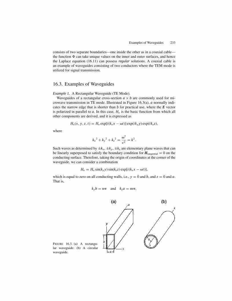
Examples of Waveguides 233
consists of two separate boundaries—one inside the other as in a coaxial cable—the function � can take unique values on the inner and outer surfaces, and hencethe Laplace equation (16.11) can possess regular solutions. A coaxial cable isan example of waveguides consisting of two conductors where the TEM mode isutilized for signal transmission.
16.3. Examples of Waveguides
Example 1. A Rectangular Waveguide (TE Mode).Waveguides of a rectangular cross-section a × b are commonly used for mi-
crowave transmission in TE mode. Illustrated in Figure 16.3(a), a normally indi-cates the narrow edge that is shorter than b for practical use, where the E vectoris polarized in parallel to a. In this case, Hx is the basic function from which allother components are derived, and it is expressed as
Hx (x, y, z, t) = Ho exp[i(kx x − �t)] exp(ik y y) exp(ikzz),
where
kx2 + ky
2 + kz2 = �2
c2= k2.
Such waves as determined by ±kx , ±ky, ±kz are elementary plane waves that canbe linearly superposed to satisfy the boundary condition for Htangential = 0 on theconducting surface. Therefore, taking the origin of coordinates at the corner of thewaveguide, we can consider a combination
Hx = Ho sin(ky y) sin(kzz) exp[i(kx x − �t)],
which is equal to zero on all conducting walls, i.e., y = 0 and b, and z = 0 and a.That is,
kyb = n� and kza = m�,
FIGURE 16.3. (a) A rectangu-
lar waveguide. (b) A circular
waveguide.

234 16. Guided Waves
where m and n are 0 or ± integers, and
kc2 = ky
2 + kz2 =
(m�
a
)2
+(n�
b
)2
.
Using this result, the transversal vectors calculated with (16.11) are given by
Ht = − ikx ky
kc2
Ho exp[i(kx x − �t)][cos(ky y) sin(kzz)j + sin(ky y) cos(kzz)k]
and
Et = − i�oky
kc2
Ho exp[i(kx x − �t)][sin(ky y) cos(kzz)j − cos(ky y) sin(kzz)k].
Specified by indexes m and n, a particular mode is denoted by TEmn. In practice,those specified by low indexes are in use; for example, in TE10 mode for m = 1and n = 0, we have �c = 2a, as already discussed in Section 16.1. Waves of awavelength shorter than the cut-off �c can be transmitted through such an “over-sized” waveguide, but its energy may be dispersed into many modes of allowedtransmission. In this context it is a normal practice that a waveguide is operated fora wavelength in the range �c (TE10) > � > �c (TE20), i.e., 2a > � > a, to avoidsuch an energy loss.
Field-lines of E and H in TE10 mode are sketched at a given x and t in Figure 16.4,showing that the pattern consists of well-defined magnetic loops and concentratedelectric flux periodically at every 1�g in the xy- and xz-planes, respectively.
The TM mode in a rectangular waveguide can be discussed similar to the TE.In this case we can start with the longitudinal component Ex that is expressed inexactly the same way as Hx for a TE mode. Namely,
Ex = Eo sin(ky y
)sin (kzz) exp [i (kx x − �t)] ,
which satisfies Ex = 0 at the boundaries at y: z = 0, a, and b, resulting in therelations
kyb = n� and kza = m�,
FIGURE 16.4. The TE10 mode in a rectangular waveguide: (a) E lines; (b) H lines.

Examples of Waveguides 235
leading to the formula
kc2 = ky
2 + kz2 =
(m�
a
)2
+(n�
b
)2
,
which is the same as TE mode. However, in TM mode the transversals Et and Ht
are expressed in a form different from TE, and their derivation is left for interestedreaders as an exercise problem.
Example 2. A Circular Waveguide.In a circular waveguide sketched in Figure 16.3(b), propagating waves can also
be in TE and TM modes. In this case, because the y and z directions are identicalby symmetry, a linearly polarized wave along the z direction, for example, can beeasily mixed with a y-polarized wave, if there is a perturbing obstacle in the guide.However, because a �= b in a rectangular waveguide, the TE10 and TE01 modes areclearly distinct from each other. In this context, a circular waveguide is adequatefor practical use; nevertheless, it is an interesting theoretical problem.
For the TM mode we solve the Helmholtz equation for Ex , which can be writtenwith cylindrical coordinates (� , �, x), that is,
1
�
∂
∂�
(�
∂ Ex
∂�
)+ 1
� 2
∂2 Ex
∂�2+ ∂2 Ex
∂x2− 1
c2
∂2 Ex
∂t2= 0.
Writing that Ex (� , �, x, t) = Eo R(� )�(�) exp[i(kx x − �t)], this equation can beseparated into ordinary differential equations for individual variables:
d2�
d�2= −m2�
and
1
�
d
d�
(�
dR
d�
)+ m2
� 2R + (
k2 − kx2)
R = 0,
where m = 0, ± integers. Letting k2 − kx2 = kc
2, the equation for R(� ) can bewritten as the standard form of the Bessel equation with a characteristic parameterkc, i.e.,
d
d�
(�
dJm (kc� )
d�
)+
(kc
2� − m2
�
)Jm (kc� ) = 0,
where R(� ) = Jm(kc� ) is Bessel’s function of the mth order. Accordingly, thepropagating mode is generated from Ex as given by
Ex (� , �, x, t) = Eo Jm (kc� ) exp (±im�) exp [i (kx x − �t)] .
Applying the boundary condition Etangential = 0 at � = a on the inner surface of

236 16. Guided Waves
FIGURE 16.5. Bessel’s functions Jo(kc� ), J1(kc� ), and J2(kc� ). These are periodic, and Jo(0)
�= 0, but J1(0) = 0 and J2(0) = 0.
the tube, we have Jm(kca) = 0, from which kc can be numerically determined asroots. Figure 16.5 shows curves of the Bessel functions that are quasi-oscillatory,having many values of kca for Jm to vanish. Table 16.1 shows such roots forrepresentative m = 0, 1, and 2. Indexing these sequential roots of Jm = 0 asrmn, i.e., Jm(rmn) = 0, we can specify propagating modes as TMmn that are sig-nified by characteristic kc = rmn/a or by the corresponding cut-off wavelength�c = 2�a/rmn.
For transversal components, we calculate gradt Ex ≡ u�∂ Ex
∂�+ u�
1
�
∂ Ex
∂�, and
obtain
(E�
)mn
= ikx Eo
kc2
dJm(kc� )
d�exp (±im�) exp [i(kx x − �t)] ,
(E�)mn = ∓ imkx
kc2
Jm(kc� )
�exp (∓im�) exp [i(kx x − �t)]
TABLE 16.1. Roots of Jm(xn) = 0 and J ′m(xn) = 0.
Roots of Jm(xn) = 0
m 0 1 2 3
n = 1 3.832 1.841 3.054 4.021
2 7.016 5.331 6.076 8.015
3 10.173 8.536 9.969 11.346
Roots of J ′m(xn) = 0
m 0 1 2 3
n = 1 2.405 3.832 5.136 6.380
2 5.520 7.016 8.417 9.761
3 8.653 10.173 11.620 13.015
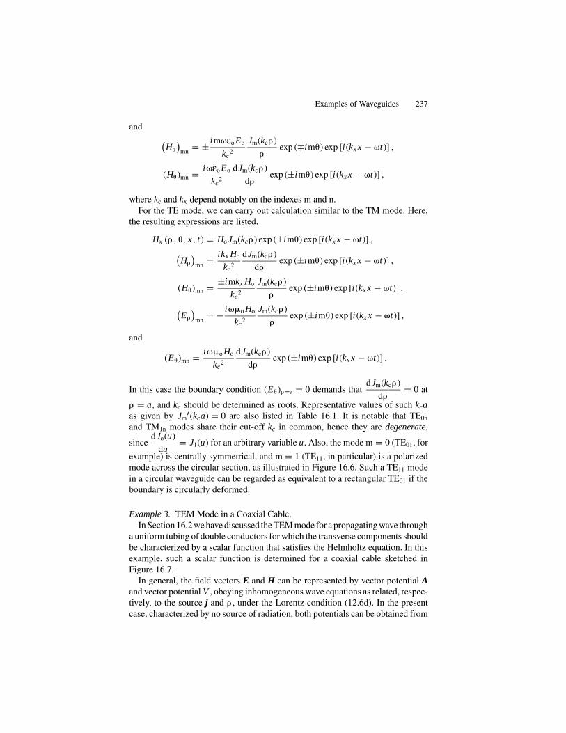
Examples of Waveguides 237
and
(H�
)mn
= ± im�εo Eo
kc2
Jm(kc� )
�exp (∓im�) exp [i(kx x − �t)] ,
(H�)mn = i�εo Eo
kc2
dJm(kc� )
d�exp (±im�) exp [i(kx x − �t)] ,
where kc and kx depend notably on the indexes m and n.For the TE mode, we can carry out calculation similar to the TM mode. Here,
the resulting expressions are listed.
Hx (� , �, x, t) = Ho Jm(kc� ) exp (±im�) exp [i(kx x − �t)] ,
(H�
)mn
= ikx Ho
kc2
dJm(kc� )
d�exp (±im�) exp [i(kx x − �t)] ,
(H�)mn = ±imkx Ho
kc2
Jm(kc� )
�exp (±im�) exp [i(kx x − �t)] ,
(E�
)mn
= − i�o Ho
kc2
Jm(kc� )
�exp (±im�) exp [i(kx x − �t)] ,
and
(E�)mn = i�o Ho
kc2
dJm(kc� )
d�exp (±im�) exp [i(kx x − �t)] .
In this case the boundary condition (E�)�=a = 0 demands thatdJm(kc� )
d�= 0 at
� = a, and kc should be determined as roots. Representative values of such kcaas given by Jm
′(kca) = 0 are also listed in Table 16.1. It is notable that TE0n
and TM1n modes share their cut-off kc in common, hence they are degenerate,
sincedJo(u)
du= J1(u) for an arbitrary variable u. Also, the mode m = 0 (TE01, for
example) is centrally symmetrical, and m = 1 (TE11, in particular) is a polarizedmode across the circular section, as illustrated in Figure 16.6. Such a TE11 modein a circular waveguide can be regarded as equivalent to a rectangular TE01 if theboundary is circularly deformed.
Example 3. TEM Mode in a Coaxial Cable.In Section 16.2 we have discussed the TEM mode for a propagating wave through
a uniform tubing of double conductors for which the transverse components shouldbe characterized by a scalar function that satisfies the Helmholtz equation. In thisexample, such a scalar function is determined for a coaxial cable sketched inFigure 16.7.
In general, the field vectors E and H can be represented by vector potential Aand vector potential V , obeying inhomogeneous wave equations as related, respec-tively, to the source j and � , under the Lorentz condition (12.6d). In the presentcase, characterized by no source of radiation, both potentials can be obtained from

238 16. Guided Waves
FIGURE 16.6. Transmission
lines with two conductors. (a)
A coaxial cable. (b) Parallel
cylinders.
homogeneous wave equations, as restricted by
divA + 1
c2
∂V
∂t= 0. (12.6d)
In a TEM mode the E and H vectors are both transversal and in the yz-plane,while signified by a longitudinal phase kx x − �t . Accordingly, we may writeV = Voexp[i(kx x − �t)] and Ax = Aoexp[i(kx x − �t)], leaving Ay and Az asfunctions of y and z. Then (12.6d) can be expressed as
∂ Ay
∂y+ ∂ Az
∂z+ i
(kx Ao − �Vo
c2
)exp [i(kx x − �t)] = 0.
The third term vanishes when kx = �
c= k, provided that Ao = Vo
c, and we obtain
∂ Ay
∂y+ ∂ Az
∂z= 0 and Ax = Vo
cexp [i(kx − �t)] .
Therefore, from the basic relation B = curl A,
By = −∂ Ax
∂z= −1
c
∂Vo
∂zand Bz = −∂ Ax
∂y= −1
c
∂Vo
∂y,
hence the scalar function Vo/oc can be considered responsible for the transversevector Ht. Further, as Ay and Az are time-independent, we can write Et = −gradtVo
in the yz-plane. Thus, for a TEM mode, the scalar potential V = Voexp[i(kx −�t)]
FIGURE 16.7. TE11 and TE01 modes
in a cylindrical waveguide.

Examples of Waveguides 239
is essential for propagation at � = ck, although the transversal fields are differentfrom the free plane waves.
To determine the transversal field, we need to solve the Helmholtz equation
ΔtVo = 0.
For a coaxial cylindrical cable, it is expressed as
1
�
∂
∂�
(�
∂Vo
∂�
)+ 1
� 2
∂2Vo
∂�2= 0.
Practically, the most important mode has a circular symmetry, being independentof �. In this case we only deal with the equation
d
d�
(�
dVo
d�
)= 0,
whose solution is expressed as
Vo(� ) = c1 ln � + c2,
where c1 and c2 are constants of integration. Because of the two separate conductors(radii a < b), the potential is signified by the potential difference �V = Vo(b) –Vo(a) as c1 = �V /ln(b/a), and
E� = − kc1
�εoo
exp [i(kx − �t)]
�, E� = 0
and
H� = 0, H� = − c1
o
exp [i(kx − �t)]
�.
A coaxial cable is useful for applications in a wide range of frequencies, as there isno cut-off in the TEM mode. However, because of double conductors, the attenua-tion due to conductive loss of energy is relatively heavier than it is for waveguidesof a single conductor.
15Waves and Boundary Problems
15.1. Skin Depths
Although a static conductor is characterized by E = 0, the electric field E canpenetrate into a conducting medium if it is varying as a function of time. In aconductor, charge carriers are mobilized by an applied electric field so that currentsflow through a conductor under time-dependent conditions. Distributed currents,called eddy currents, flow at high densities in the close vicinity of surfaces to certaindepth, called the spin-depth. In free space, electromagnetic waves are reflected bydielectric boundaries as well as conducting surfaces where surface currents play asignificant role.
A magnetic field can also penetrate into a conductor. In a uniform wire ofconductivity σ of circular cross-section of radius R, the magnetic field origi-nates from a current through the wire. For a magnetic field outside a current, wehave considered a thin wire with the Ampere law, but the magnetic field alsoexists inside the wire corresponding to the distributed current. Such a conduc-tion current is related to an applied field E as described by the Ohm relationj = σE, and it is also related to the magnetic field H by the Maxwell equations,that is
curl H = j + ε∂ E∂t
and curlE = −μ∂ H∂t
, (15.1)
where constants ε and � of the conductor can be assumed as close to ε0 and �0 invacuum space.
Consider a sinusoidal current I = I0 exp(i�t) along the z-axis of a long cylin-drical conductor. Using cylindrical coordinates (r, �, z), the circular component ofthe magnetic field H� inside and outside the conductor is, by symmetry, a functionof radius r , varying at the frequency �; and the total current density is contributedby conduction and displacement currents and hence given by �Ez + i�εEz , whereEz is related to H� . Under normal circumstances however, the second term is neg-ligibly small as compared with the first. A metallic conductivity � is typically ofthe order of 108�−1/m, which is much greater than �ε even at a frequency � in
214
Skin Depths 215
MHz. In this case, combining two equations in (15.1), we write
curl j = −i���o H, (i)
and
curl(curl j) = �2 j, where �2 = −���o. (ii)
Considering that the H vector is dominated by H� , the corresponding currentdensity is signified only by jz(r ), where r is the radial coordinate, as determinedby (i), i.e.,
H� = 1
�2r
d
dr(r jz) , (iii)
and from (ii) we have
− d
dr
[1
r
d
dr(r jz)
]= �2 jz .
This equation can be expressed as
d2 jzdr2
+ 1
r
d jzdr
+(
�2 − 1
r2
)jz = 0,
which is a Bessel’s equation, whose solution can be written as
jz (r ) = jo J1(�r ) . (iv)
Using (iv) in (iii), we have
H� = 1
�2
(jzr
+ d jzdr
)= jo
�2
(J1(�r )
r+ dJ1(�r )
dr
)= jo
�Jo(�r ) , (v)
where the last expression was obtained by a recurrence formula for Bessel func-tions. This expression of H� in (v) must be consistent with the Ampere law at
r = R, and hence jo = �I
2�R Jo(�R). Therefore, from (iv) and (v) the current
density and magnetic field inside the wire are expressed by
jz(r ) = �I
2�R
J1(�r )
Jo(�R)and H� = I
2�R
Jo(�r )
Jo(�R)for r < R,
respectively.From (ii), the constant � is a complex parameter, and written as
� = 1 − i
�, where � =
√2
���o
(vi)
For r � � the current density jz(r , t) can be expressed asymptotically as
jz(r, t) = I
2�R�exp
(r − R
�
)exp
[i
(�t + �
4+ R − r
�
)],

216 15. Waves and Boundary Problems
and the magnetic field is
H� = I
2�Rexp
(r − R
�
)exp
[i
(�t + R − r
�
)].
In this approximation, the parameter �(0 < � < R) signifies the effective depthto which the current density must penetrate into the conductor, which is, however,limited to a thin area close to the surface of radius R. It is noted that at r = 0,jz = 0, but Hz �= 0, as given by the Bessel functions J1(�r ) and Jo(�r ), takingzero and non-zero values at r = 0, respectively.
15.2. Plane Electromagnetic Waves in a Conducting Medium
In this section, we consider a plane electromagnetic wave propagating through auniform medium characterized by a conductivity �. Mobile electrons dominateconducting properties, although the wave’s dielectric and magnetic properties de-termined, respectively, by ε and � depend on the host medium not including itselectrons, which are insignificant in most conductors. In normal conductors theMaxwell equations are written as
curl H = �E + εo
∂ E∂t
and curl E = −�o
∂ H∂t
.
In this case, it is convenient to use the vector potential A instead of E and H,namely
E = −∂ A∂t
and H = 1
�o
curl A,
and we obtain the equation
∇2 A − εo�o
∂2 A∂t2
− �o�∂ A∂t
= 0. (15.2)
For a plane wave, writing A(r , t) = Ao exp[i(k . r − �t)] in (15.2), we obtain therelation
−k2 + �2εo�o + i��o � = 0.
Hence, the wave vector k is a complex variable, that is, k = k ′ + ik ′′, where thereal and imaginary parts k ′ and k ′′ are expressed by the relations
k ′2 − k ′′2 = �2εo�o and 2k ′k ′′ = ��o�.

Plane Electromagnetic Waves in a Conducting Medium 217
Solving these equations for k ′ and k ′′, we obtain
k ′ = �
√εo�o
2
{1 +
√1 +
(�
�εo
)2}1/2
and
k ′′ =√
εo�o
2
{√1 +
(�
�εo
)2
− 1
}1/2
.
For a normal conductor, the condition � � �εo an be applied at a typical frequency�, so that these k ′ and k ′′ can be approximately given by
k ′ ≈ k ′′ ≈ �
√εo�o
2
�
�εo
=√
���o
2. (15.3)
In this case, the vector potential can be written as
A(r , t) = Ao exp(−k′′. r ) exp[i(k′. r − �t)], (15.4)
indicating that the amplitude decreases as propagating along the direction of k. Wecan define a characteristic distance for the amplitude decay by
� = 1
k ′′ =√
2
���o
,
which is identical to the skin depth defined in Section 15.1.Writing k = (k ′ + ik′′)u = k ′(1 + i)u, where the unit vector u signifies a linearly
polarized wave, the field vectors can be calculated for the vector potential of (15.3),that is,
H(r , t) = curl A�o
= ik ′ (1 + i)
�o
u × A (r , t) ≈ i
√��
�o
exp
{�i
4[u × A (r , t)]
}
= i
√��
�o
(u × Ao) exp(−k′′. r
)exp
[i(
k′. r − �t + �
4
)]
and
E(r , t) = i�A(r .t) = i�Ao exp(−k′′. r ) exp[i(k′. r − �t)].
It is noted that these amplitudes are related as
√ εo
�o
|E||H| =
√�εo
�� 1, and hence
|E| � |H| in normal conductors. In fact, by considering � = ∞, an idealized con-ductor may be characterized by E = 0, as in a static case, even at high frequencies.In this context we can set up boundary conditions for the electromagnetic field tosatisfy E = 0 on conducting surfaces, which is consistent to assuming the skindepth � as zero.

218 15. Waves and Boundary Problems
15.3. Boundary Conditions for Propagating Waves
The plane wave is a useful model for electromagnetic radiation propagating awayfrom the source. In practice, a plane wave propagates through media of conductingand non-conducting materials for which the media boundaries play a significantrole in transmitting energies to carry information by the wave. In the presence ofboundaries waves can no longer be “free” to propagate, as in isolated space, andthe field should necessarily be modified, as expressed by a linear combination ofappropriate waves to satisfy boundary conditions.
Because of a high conductivity �, a normal conductor surface can be character-ized by a thin layer of the skin depth �, where eddy currents flow to keep the fieldfrom penetrating deeper, whereas the boundary between two uniform dielectricmaterials 1 and 2 is characterized by different dielectric constants ε1 and ε2. Suchboundaries can be expressed by a mathematical surface, but physically signifiedby surface currents and charges, although on dielectric boundaries no boundarycharges are normally considered.
The basic equation curl H = j should determine the surface condition for theH field that arises from a surface current. Figure 5.1 shows a flat conductingsurface, where we consider a rectangular path for integration perpendicular to thecurrent j. Here, the lengths of 1-2 and 3-4 are denoted as l, and those of 2-3 and4-1 are 2�, where the surface current is assumed to flow through the bottom halfof this rectangular path. Denoting the rectangular area by A, the current can beexpressed as j(l�) = K l, where K = j� describes the surface density. For theequation curl H = j , the left side can be calculated as (curl H) . A = (n × H)lbecause the H vector is all zero, except for the path 1-2 above the conductor. Hence,as the boundary condition we obtain the relation
n × H = K . (15.4a)
Accordingly, the tangential component of H is discontinuous across the surface.Applying curl E = 0 to a similar path, we can obtain another condition
n × E = 0 (15.4b)
for the E vector. This formula (15.4b) indicates that the tangential component ofE should be equal to zero at any outside point of conducting surface.
FIGURE 15.1. A boundary
condition for tangential
components of H vectors
on a conducting surface.
n × (H1 − H2) = K , where
K = j� is the surface current
density, n the normal vector,
and � the skin depth.
Reflection from a Conducting Boundary 219
Next, we consider a pill-box shaped short cylindrical volume across a conductingboundary in parallel with its flat top and bottom, similar to Figure 3.5, where thebasic equations div B = 0 and div D = are analyzed in integral form using theGauss theorem. Assuming that the side area is negligible as compared with the topand bottom, we obtain that the normal component of B is continuous, and hence
(Hn)1 = (Hn)2, (15.4c)
where we considered that �1 = �2. Inside a conducting medium 2, (Hn)2 is equalto zero, except in the skin depth, and hence, H should be tangential to the surface.
In contrast, because of distributed charge , the E vector cannot be continuous,as we already discussed for the static case; namely from (Dn)1 = �, we have(En)1 = �/εo.
Summarizing these conditions, for propagating waves the conducting surfacedemands the boundary conditions that
Etangential = 0, Enormal = �/εo; Htangential = K and Hnormal = 0. (15.5)
It is clear that such conditions cannot be met by a single propagating wave specifiedby the wavevector k for which a superposition with another wave at different k′ isrequired, resulting in a reflected wave from the surface.
On a dielectric boundary, in contrast, two different dielectric constants ε1 andε2 are explicit, for which we can write conditions
ε1(En)1 = ε2(En)2 and (Hn)1 = (Hn)2, (15.6a)
assuming that �1 = �2. On the other hand, as long as the absence of boundarycurrent and charge signifies the dielectric properties, tangential components Et
and Ht should be continuous. Namely,
(Et)1 = (Et)2 and (Ht)1 = (Ht)2. (15.6b)
Therefore, the boundary conditions are involved only in discontinuous En, asexpressed by (15.6a), and the H vector has nothing to do with a dielectric boundary.However, the continuity of Et in (15.6b) cannot be disregarded, because at adielectric boundary the E vector is modified as specified by discontinuous En
together with continuous Et.
15.4. Reflection from a Conducting Boundary
Although expressible by optical analogy, the reflection and refraction of wavesneed to be interpreted in terms of electromagnetic propagation at boundaries. Fora free wave we deal with the field vectors E and H in orthogonal relation with thewave vector k as given by (13.4) and (13.5). In optics, on the other hand, thesevector relations represent polarization of light to indicate a direction of the electricfield. For a plane electromagnetic wave such a polarization arises from the sourcecurrent, and the natural optical light is normally “unpolarized,” originating fromatomic or molecular transitions in r and om phases.
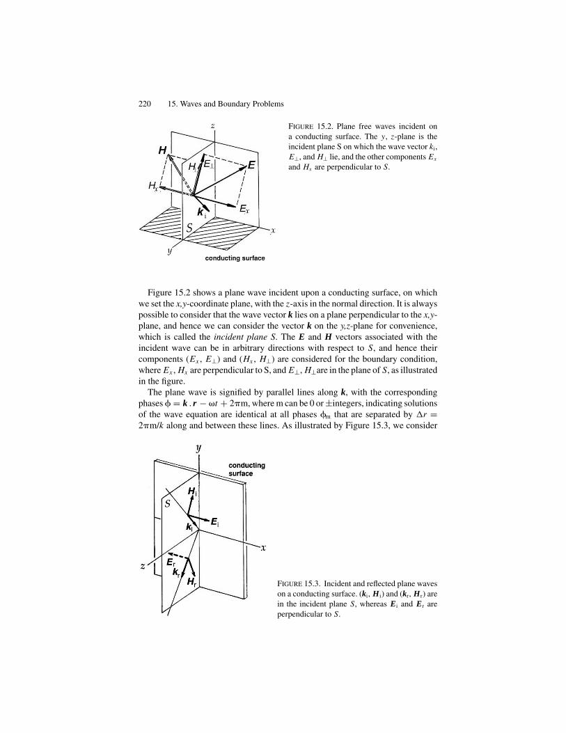
220 15. Waves and Boundary Problems
FIGURE 15.2. Plane free waves incident on
a conducting surface. The y, z-plane is the
incident plane S on which the wave vector ki,
E⊥, and H⊥ lie, and the other components Ex
and Hx are perpendicular to S.
Figure 15.2 shows a plane wave incident upon a conducting surface, on whichwe set the x,y-coordinate plane, with the z-axis in the normal direction. It is alwayspossible to consider that the wave vector k lies on a plane perpendicular to the x,y-plane, and hence we can consider the vector k on the y,z-plane for convenience,which is called the incident plane S. The E and H vectors associated with theincident wave can be in arbitrary directions with respect to S, and hence theircomponents (Ex , E⊥) and (Hx , H⊥) are considered for the boundary condition,where Ex , Hx are perpendicular to S, and E⊥, H⊥are in the plane of S, as illustratedin the figure.
The plane wave is signified by parallel lines along k, with the correspondingphases = k . r − �t + 2�m, where m can be 0 or ±integers, indicating solutionsof the wave equation are identical at all phases m that are separated by �r =2�m/k along and between these lines. As illustrated by Figure 15.3, we consider
FIGURE 15.3. Incident and reflected plane waves
on a conducting surface. (ki, Hi) and (kr, Hr) are
in the incident plane S, whereas Ei and Er are
perpendicular to S.

Dielectric Boundaries 221
an incident plane wave (Ei, Hi, ki) and a reflected wave (Er, Hr, kr), which can belinearly combined at the same phase to satisfy the boundary conditions (15.5) onthe conducting surface. Using notation of Figure 15.2, if we take Eix = −Erx , thecorresponding Hi⊥ and Hr⊥ can both be in the incident plane, making the vectorsum Hi⊥ + Hr⊥ = K , as specified by the boundary condition (15.5). In this case,the wavevector kr of the reflected wave is on the incident plane as symmetrical toki with respect to the z-axis that is normal to the conducting surface. Angles �i,�r that vectors ki, kr make with the normal to the conducting surface n are calledthe angle of incidence and angle of reflection, respectively, for which we shouldconsider that
�i = �r (15.7)
to satisfy the boundary conditions. Equation (15.7) represents the law of reflection.The oscillating surface current density K is responsible for the reflected wave. If
the incident Hi wave is polarized along the x-axis, Hr must be chosen as Hi + Hr =0, implying that K = 0, hence generating no reflection. Accordingly, to obtainreflection, the incident wave should have a component along the x-axis. In thiscontext, if Ei is arbitrarily polarized, only its x component is responsible forreflection. Consequently, a natural light reflected from a conducting surface islinearly polarized.
In the above treatment the incident and reflected waves are mixed in phase andconnected with the penetrated wave at the conducting boundary. As we discussedin Section 15.2, the conductivity � makes the penetration limited to the skindepth �. During penetration, the electromagnetic energy is converted to heat in theconducting layer.
15.5. Dielectric Boundaries
Dielectric boundaries are signified by different dielectric constants characterizedby no surface charges and currents under normal circumstances. In this case,the general boundary conditions (15.6a) and (15.6b) can be rephrased by con-tinuity of Etangential and Dnormal. Magnetic properties are insignificant for mostdielectrics, which are specified by the same magnetic permeability �o as in avacuum.
More important, at normal boundaries of isotropic dielectric media there is noparticular mechanism for rotating the polarization vector. Therefore, the vector E,and hence D, does not change direction at boundaries; reflected and refracted wavesboth propagate with no change in polarization in the plane of incidence. As is clearfrom the illustration in Figure 15.2, where (Ex , Hx ) and (E⊥, H⊥) sin � representtangential and normal components of (E, H), respectively. Therefore, as indicatedby such boundary conditions, the wave vectors ki, kr, and kp for incident, reflected,and penetrated waves are all in the incident plane, as shown in Figure 15.4, where�r and �p are angles of reflection and refraction (or penetration). Thus, we have a

222 15. Waves and Boundary Problems
FIGURE 15.4. The Snell law of reflec-
tion and refraction.
relation
sin �i
sin �p
= ki
kp
= k1
k2
=√
ε1
ε2
.
For optical light, a dielectric material is specified by the refractive index that isdefined by n = √
ε/εo, and the equation
sin �1
sin �2
= n1
n2
(15.8)
is called the Snell law in geometrical optics, indicating that �1 > �2 if n1 > n2 orε1 > ε2.
If, on the other hand, n1 < n2, from the Snell law we have sin �2 = n2
n1
sin �1,
where the angle of refraction cannot be obtained unless |sin �2| ≤ 1. Therefore,in this case if the incident angle �1 is larger than a specific angle �B determined
byn2
n1
sin �B ≤ 1, there is no refraction, as shown in Figure 15.5. Such an angle
defined by �B = sin−1 n1
n2
is known as the Brewster angle, and the wave is totally
reflected if an incidence angle exceeds �B. At optical frequencies waves propagatenormally as a collimated beam carrying a well-defined energy; these waves aresplit into reflected and refracted beams at the boundary. If �1 > �B, in particular,all the beam energy is carried away in the medium 1 by total reflection. In laseroptics light can be transmitted through an insulating cable of dielectric materialwhere ε > εo with virtually no loss of energy due to the total reflection conditionon the dielectric wall. Such a cable, known as fiberoptic, is widely used for opticalcommunication in modern technology.

The Fresnel Formula 223
FIGURE 15.5. Total reflection
and the Brewster angle �B.
15.6. The Fresnel Formula
In Section 15.4 we considered the phase of a wave variable for boundary conditionsin order to determine directions for propagation. In this section we derive therelations among amplitudes of incident, reflected waves, and refracted waves at adielectric boundary, which are known collectively as the Fresnel formula in optics.
Figure 15.6 shows the field vectors of waves in the vicinity of a dielectricboundary, where the incident wave is polarized in such a way that the E vectoris perpendicular to the plane of incidence S. In this case, if we take the z-axisparallel to the normal to the conducting surface, the x-axis is in parallel to theE vector. A wave for such a specific polarization shall be called the “mode I,” todistinguish it from another mode, “mode II,” discussed shortly. Since the boundaryconditions for these E and H vectors are determined by continuity of the tangential
FIGURE 15.6. Directions of (k, E, H) for incident, reflective, and refractive plane waves at
a dielectric boundary.

224 15. Waves and Boundary Problems
components, we can write
Ei − Er = Ep along the x direction (i)
and
Hi cos �i − Hr cos �r = Hp cos �p along the z direction. (ii)
These plane electromagnetic waves are characterized separately by
Ei
Hi
= ��o
ki
,Er
Hr
= ��o
kr
andEp
Hp
= ��o
kp
,
and the H fields in (ii) can be expressed as
ki (Ei − Er) = kp Ep. (iii)
Using the law of reflection, i.e., �i = �r in (i), (ii), and (iii), we obtain(Er
Ei
)I
= n1 cos �i − n2 cos �p
n1 cos �i + n2 cos �p
and
(Ep
Ei
)I
= 2n1 cos �i
n1 cos �i + n2 cos �p
(15.9a)
for mode I, where n1 and n2 given by√
ε1/εo and√
ε2/εo are refractive indexes
of the media 1 and 2. Further applying the Snell law, i.e.,n1
n2
= sin �i
sin �p
, these
expressions can be written as(Er
Ei
)I
= sin(�p − �i
)sin
(�p + �i
) and
(Ep
Ei
)I
= 2 sin �p sin �i
sin(�p + �i
) . (15.9b)
For mode II we consider that the boundary conditions can be specified as
Hi − Hr = Hp along the x-axis
and
Ei cos �i − Er cos �r = Ep cos �p in the y,z-plane.
After a similar manipulation to mode I, we can derive the following relations formode II, that is,(
Er
Ei
)II
= n2 cos �i − n1 cos �p
n2 cos �i + n1 cos �p
and
(Ep
Ei
)II
= 2n1 cos �i
n2 cos �i + n1 cos �p
,
(15.10a)
which are very similar to (15.9a), but noted that n1 and n2 are exchanged in (15.9a).Using the Snell law, the equation (15.10a) is led to a form different from (15.9b).Namely,(
Er
Ei
)II
= − tan(�i − �p
)tan
(�i + �p
) and
(Ep
Ei
)II
= sin(�i + �p
) − sin(�i − �p
)sin
(�i + �p
)sin
(�i − �p
) .
(15.10b)
Equations (15.9) and (15.10) are known as the Fresnel formula in optics.

The Fresnel Formula 225
It is interesting to note that in mode II the amplitude of reflection Er vanishes,if �i + �p → �/2, and hence such a specific incident angle �i = 1� − �p is calledthe polarizing angle �P. When �i = �p, from the Snell law we can write
tan �p = n1
n2
, (15.11)
where the polarizing angle is determined by the ratio of refractive indexes, but not
exactly the same as the Brewster angle �B = sin−1
(n1
n2
).
For the perpendicular incidence,we have �i = �r = �p, and the Fresnel formulacan be written specifically as(
Er
Ei
)I,II
= ±n1 − n2
n1 + n2
and
(Ep
Ei
)I,II
= 2n1
n1 + n2
, (15.12)
indicating that if n1 < n2 the reflected wave is out of phase with respect to theincident phase.
Part 4Coherent Waves and Radiation Quanta
Generated by oscillatory charges, the electromagnetic wave propagates at the speedof light, as described by the Maxwell theory. Transmitting energy in the distance, itis utilized for telecommunication in a wide range of frequencies, for which intenseamplitudes are required. Prompted by pressing demands since WWII, significantadvances have been achieved in manipulating microwaves and coherent opticalradiation, resulting in today’s advanced technologies and spectroscopic studies onmodern materials. Among recent advances, coherent radiation has opened up alarge area of applications beyond the traditional scope of classical electromag-netism.
In Part 4, we duscuss guides waves and resonant cavities as indispensable devicesin modern electronics. At optical frequencies, we particularly encounter the limit ofclassical theory, regarding the coherence problem. It is important for us to realizedthat there is a significant limit for the classical Maxwell theory.
241

17Waveguide Transmission
17.1. Orthogonality Relations of Waveguide Modes
In the previous chapter, we discussed TE and TM modes of electromagnetic prop-agations in a rectangular waveguide, and a TEM mode in a coaxial cable. In awaveguide, axial components of E or H vectors behave like scalar variables ofthe phase of propagation, and in a coaxial cable the uniaxial vector potential Aplays such a role as a scalar variable. Thus, transversal fields depend on the typeof waveguide; on the other hand, the axial component plays essential role forpropagation.
Summarizing the previous results, TE and TM modes in a rectangular waveguideare expressed as
(�t + k2
c
)Hx = 0, Ht = ikx
k2c
gradt Hx , and Et = − ik Zo
k2c
[i × gradt Hx ] for TE
and
(�t + k2
c
)Ex = 0, Et = ikx
k2c
gradt Ex , and Ht = ik
Zok2c
[i × gradt Ex ] for TM,
where
k2c =
(m�
a
)2
+(n�
b
)2
, m and n are 0 or integers.
Although specified by two indexes (m, n), each waveguide mode is characterizedby kc that is a single parameter related to m and n. Therefore, in the following wedistinguish different modes by the single index kc when discussing orthogonalityrelations.
We show that any two modes, indexed by different α and β are mutually orthog-onal. Such waveguide modes can be represented by an effective scalar function,and therefore we consider a function ϕ1gradtϕ2 composed of two scalars ϕ1 andϕ2 and its divergence, i.e.,
divt(ϕ1gradtϕ2) = (gradtϕ1) · (gradtϕ2) − ϕ1�tϕ2.
243
244 17. Waveguide Transmission
Calculating the flux of two-dimensional vector ϕ1gradtϕ2 with the Gauss theorem,we have∫v
div(ϕ1gradtϕ2)dv =∫S
ϕ1
∂ϕ2
∂ndS =
∫v
{(gradtϕ1) · (gradtϕ2) − ϕ1�tϕ2}dv,
where dv = dSdx represents the volume element taken along the waveguide, anddS is the differential element on the cross-section S. Therefore, from the lastequation we have
∮C
ϕ1
∂ϕ2
∂nds =
∫S
{(gradtϕ1)(gradtϕ2) − ϕ1�tϕ2}dS.
Taking the boundary conditions �1,2 = 0 and∂ϕ1,2
∂n= 0 into account, the line
integral on the left side vanishes, and we obtain
∫S
(gradtϕ1) · (gradtϕ2)dS =∫S
ϕ1�tϕ2 dS. (i)
We consider ϕ1 = Hx1 and ϕ2 = Hx2, distinguishing them by kc1 and kc2,respectively, thereby expressing the relation (i) as
k2c1k2
c2
kx1kx2
∫S
Ht1.Ht2dS = −k2c2
∫S
Hx1 Hx2dS.
It is clear that this relation is correct regardless of values of these kc, kx , providedthat the orthogonality relations
∫S
Ht1.Ht2dS = 0 and
∫S
Hx1 Hx2dS = 0 (17.1a)
hold for different modes 1 and 2. Such a relation can also be derived for E vectorsbecause Et = Zo Ht with a constant phase factor, and hence we can write
∫S
Et1.Et2dS = 0 (17.1b)
for different modes 1 and 2. Also, from the relation kx1i(Et1 × Ht2) = Zo Ht1 · Ht2,we can show that vectors i, Et1, and Ht2 are mutually orthogonal. These relations(17.1ab) constitute orthogonality relations for TE mode.
For TM mode we can derive similar relations to (17.1ab), namely,
∫S
Ex1 Ex2dS = 0,
∫S
Et1.Et2dS = 0 and
∫S
Ht1.Ht2dS = 0. (17.2)

Impedances 245
Further, we can show orthogonality relations hold also between TE and TM modes.For instance,
Et1(TE).Et2(TM) = − Zokkx2
k2c1k2
c2
[(i × gradt Hx1).gradt Ex2]
= Zokkx2
k2c1k2
c2
divt{Ex2curlt(iHx1)},
and hence
∫S
Et1(TE).Et2(TM)dS = Zokkx2
k2c1k2
c2
∮C
∂
∂n{Et2(curltiHt1)}.ds = 0,
because Et2 = 0 on the conducting wall. By a similar procedure, we can also showthat Ht1(TE) and Ht2(TM) are orthogonal.
Although purely mathematical, these orthogonal relations provide necessaryconditions for all waveguide modes to be linearly independent.
17.2. Impedances
So far we have discussed idealized waveguides, assuming infinite length. However,a practical waveguide is connected to an oscillator at one end, and to another objectat the other far end. Inside of a waveguide, it is practical consider, effectively, waves,propagating back and forth along the guide, which can be observed as a standingwave. We realize that such a description is useful if we can accurately define thephase of propagation for dealing with flowing energy. For such a description it issignificant that such a periodic repetition be determined within the timescale ofobservation � . In other words, such a scale � must be sufficiently long comparedwith the period of repetition.
Under normal circumstances, such waves are conveniently expressed by com-plex functions with the normalization conditions
∫S
|Et�.E∗t�|dS = 1,
∫S
|Ht�.H∗t�|dS = k2
x
k2 Z2o
, and
∫S
i.(Et� × H∗t�)dS = kx
k Zo
,
(17.3)where the * indicates complex conjugate. For practical application, the TE10 modeis employed as the principal mode, although the above argument can be appliedto any other mode.
A guided wave consists of longitudinal and transversal components of fieldvectors with respect to the x-axis. It is convenient to express it as the superpositionof forward and backward waves, both being characterized by longitudinal andtransversal components, (Ex , Hx ) and (Et, Ht), respectively. Therefore, for the

246 17. Waveguide Transmission
principal mode, we write
E = Et {A exp [i(kx x − �t)] + B exp [i(−kx x − �t)]}+ iEx {A exp [i(kx x − �t)] − B exp [i(−kx x − �t)]}
and
H = Ht {A exp [i(kx x − �t)] − B exp [i(−kx x − �t)]}+ iHx {A exp [i(kx x − �t)] + B exp [i(−kx x − �t)]} , (17.4)
where the phase −kx x − �t signifies the backward wave, but the coefficient B isleft undetermined, unless the terminal object is specified. Generally, the field ismore complex than (17.4), but at a distant point from the terminals, the backward(or reflected) wave is expressed approximately by the same principal mode with aphase shift and a smaller amplitude B than A of the forward wave.
It is noted that the mode vectors Et can usually be detected by a probe insertedperpendicular to the guide, whereas the axial component Ex is not directly measur-able in practice. By this reasoning, we only need to deal with Et in the waveguide.As discussed in Chapter 16, Et and the corresponding Ht of the principal modeare linearly related by (16.8), so that we can define the ratio Zg = |Et|/|Ht| as theeffective wave impedance. From (16.8), we can write
Zg = k
kxZo, (17.5)
which is specifically called the guide impedance.Writing (17.4) at specific phases φ = kx x − �t = 2π × (0 or integer), from
(17.4) we obtain
(A + B)2 = Et.E∗t and (A − B)2 = Et.H∗
t ,
and hence
Zg = A − B
A + B.
Figure 17.1 shows two partitions installed in a waveguide, where section 2can be regarded as a working space. These partitions should have openings ofsome kind, as illustrated in Figures 17.2 and 17.3, acting as couplings betweenseparated sections. Although mathematically not so easy to represent, field-linesnear a coupling can be inferred using physical intuition from the principal modeshown in Figure 16.4. For example, Figure 17.2 shows a coupling via mag-netic field-lines of a rectangular waveguide in TE10 mode. On the other hand,Figure 17.3 shows that by extending the center conductor at the end of a coaxial
FIGURE 17.1. A uniform wave-
guide with two partitions at x =0 and x = L .
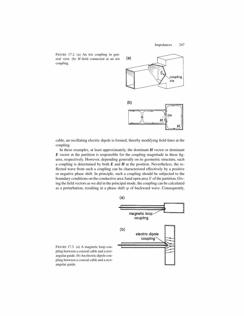
Impedances 247
FIGURE 17.2. (a) An iris coupling in gen-
eral view. (b) H -field connected at an iris
coupling.
cable, an oscillating electric dipole is formed, thereby modifying field-lines at thecoupling.
In these examples, at least approximately, the dominant H vector or dominantE vector at the partition is responsible for the coupling magnitude in these fig-ures, respectively. However, depending generally on its geometric structure, sucha coupling is determined by both E and H at the position. Nevertheless, the re-flected wave from such a coupling can be characterized effectively by a positiveor negative phase shift. In principle, such a coupling should be subjected to theboundary conditions on the conductive area Sand open area S′ of the partition. Giv-ing the field vectors as we did in the principal mode, the coupling can be calculatedas a perturbation, resulting in a phase shift ϕ of backward wave. Consequently,
FIGURE 17.3. (a) A magnetic loop cou-
pling between a coaxial cable and a rect-
angular guide. (b) An electric dipole cou-
pling between a coaxial cable and a rect-
angular guide.

248 17. Waveguide Transmission
expressing the reflected wave with a phase shift ϕ with amplitude B, the guidedwave can logically be written as
A exp [i(kx x − �t)] + B exp [i(−kx x − �t + ϕ)]
= A exp [i(kx x − �t)]
{1 + B
Aexp [i(−2kx x + ϕ)]
}.
Writing
R = B
Aexp [i(−2kx x + ϕ)] , (17.6)
the field vectors at a given (x , t) in the waveguide are expressed by
E = Et A (1 + R) exp [i(kx x − �t)] + iEx A (1 − R) exp [i(kx x − �t)]
H = Ht A (1 − R) exp [i(kx x − �t)] + iHx A (1 + R) exp [i(kx x − �t)] .
As already mentioned, a probe is utilized for measuring transversal fields alongthe vectors Et or Ht so that we can set aside the longitudinal components Ex andHx in the following calculation.
Such a terminated waveguide is said to be “loaded” by an obstacle and repre-sented by the impedance Zx at a point x defined by the ratio
Zx = |Et|(1 + R)
|Ht|(1 − R)= Zg
1 + R
1 − R. (17.7)
At the position of an obstacle x = 0, we write (17.7) as ZL, which is called theload impedance, or the coupling impedance, in this case. Also we define Ro =BA exp (i�) at x = 0, and express (17.7) as
ZL = Zg
1 + Ro
1 − Ro
and Ro = ZL − Zg
ZL + Zg
. (17.8)
In the above, we have assumed that the waveguide is made of perfectly conduct-ing materials, however, the energy loss in the waveguide during transmission isinevitable. Although such a loss of electromagnetic energy on the conducting wallsis not a simple mathematical problem, we only deal with the rate for diminishingamplitude per length. In this case, the propagation vector k can be expressed as acomplex parameter, i.e., k = k ′ + ik ′′, where the imaginary part k ′′ describes thedecay along the guide. We can also describe the propagation by a phase � x − i�tand Rx = (B/A) exp(−2γx) to emphasize decaying propagation by � = ik, inwhich case we can write the following relation between Zx and ZL:
Zx
Zg
= ZL cosh γx − Zg sinh γx
Zg cosh γx − ZL sinh γx=
ZL
Zg
− tanh γx
1 − ZL
Zg
tanh γx, (17.9)
which is a bilinear transformation between complex variablesZx
Zg
andZL
Zg
. The
derivation of (17.9) is straightforward, but left to readers as an exercise. As an ex-treme case, we see that Zx = ZL if ZL = ±Zg, indicating that Zx = ±Zg represent

Power Transmission Through a Waveguide 249
independent waves of an equal amplitude propagating in the ±x directions. Onthe other hand, if |ZL| �= Zg we have A �= B, giving rise to a finite standing wave.
17.3. Power Transmission Through a Waveguide
In the expression (17.4) of the field vectors, by amplitude factors A and B we candescribe forward and backward waves in the waveguide, respectively represent-ing incident waves to and reflected waves from the coupling iris. However, in awaveguide the word “reflection” should indicate a group of plane waves carryingan electromagnetic energy, as interpreted by the Poynting theorem.
As a measurable quantity in the waveguide, a flow of energy should be expressedas an average over the phase in repetition, since the timescale of usual observationis much longer than 2π/� of radiation. Also, the mode vectors Et and Ht may notbe exactly in phase, for which it is logical to consider the Poynting vector E(t) ×H*(t ′) that is averaged over distributed phase �(t − t ′) = d�. Therefore, for theenergy transport in a waveguide, we write the Poynting theorem as
−dU
dt=
∫S
dS
⎡⎣ 1
2π
2π∫0
i. (E × H) d�
⎤⎦
= A2 exp(−2k ′′
x x) |1 − Rx |2
∫S
i.⟨Et × H∗
t
⟩dS, (17.10)
where S is the cross-sectional area, and the brackets 〈〉 signify the time averageover repeated periods.
For a TE mode of a rectangular waveguide, the integrand in (17.10) can beexpressed as
i · 〈Et × H∗t 〉 = 〈(i × Et) · H∗
t 〉 = �μo
2kx|Ht|2 = �μo
2kx
k2x
k4c
|gradt Hx |2,
and hence
P = �μo
2kx
∫S
|Hx |2dS.
On the other hand, the electromagnetic energy is calculated from the Poyntingtheorem ∫
S
i.⟨Et × H∗
t
⟩dS = c
∫S
u dS,
where u is the energy density
u = 1εo|Et|2 + 1μo|Ht|2 + 1μo|Hx |2
= ε
2
k2 Z2o
k4c
|i × gradt Hx |2 − μo
2
k2x
k4c
|gradt Hx |2 + μo
2|Hx |2.

250 17. Waveguide Transmission
Here, using the relation gradt Hx = k2c
ikxHx , we can write u = μo
2
k2
k2x
|Hx |2, and
hence we have the relation
P = �
kx
k2x
k2uS = c
kx
kU,
where the quantity c(kx/k) = vg is generally known as the group velocity. Wenote that the group velocity can also be derived from the relation k2 = k2
c + k2x in
Figure 16.2, where
vg = d�
dkx= c
kx
k. (17.11)
As stated in (17.3), for TE mode we have the relation∫S
i.⟨Et × H∗
t
⟩dS = 1
Zg
, and
hence the total power flow in the waveguide can be calculated as
PS = A2
Zg
exp(−2k ′′x x){(1 − |Rx |2) + (Rx − R∗
x )}, (17.12)
where the first term in the brackets represents powers flowing forward and back-ward in the ratio 1 : |Rx |2. On the other hand, the second term is pure imaginary,hence representing no real power flow, unless Zg has an imaginary part. Ignoringthe latter as a mathematical conjecture, we consider the attenuating flow of poweras proportional to 1 − |Rx |2.
17.4. Multiple Reflections in a Waveguide
We consider now two partitions that are typically iris couplings, between which isa “working space.” Such partitions divide the waveguide into three parts, marked1, 2, and 3 in Figure 17.1. An oscillator is connected to the left end of section 1,section 3 has an opening at the left, and the right end is at infinity. In the centerof section 2, the principal waves are reflected back and forth between the twocouplings, whereas there are incident and reflected waves in section 1.
Each sections are characterized by wave impedances Z1, Z2, and Z3 and thepartitions are located at x = 0 and x = L . If the second opening is consideredas the load impedance in the third guide, it should be Z3, assuming no reflectionin this section. Therefore, at a position x inside section 2, i.e., 0 ≤ x ≤ L , theimpedance of (17.9) in section 2 can be expressed
Zx
Z2
=Z3
Z2
− tanh(γ2x x
)
1 − Z3
Z2
tanh(γ2x x
) ,
giving Zx=L = Z3 if tanh(γ2x L
) = 0 at the second boundary. At the first boundaryx = 0, Zx=0 = Z3, which is assumed to be the same as Z1.
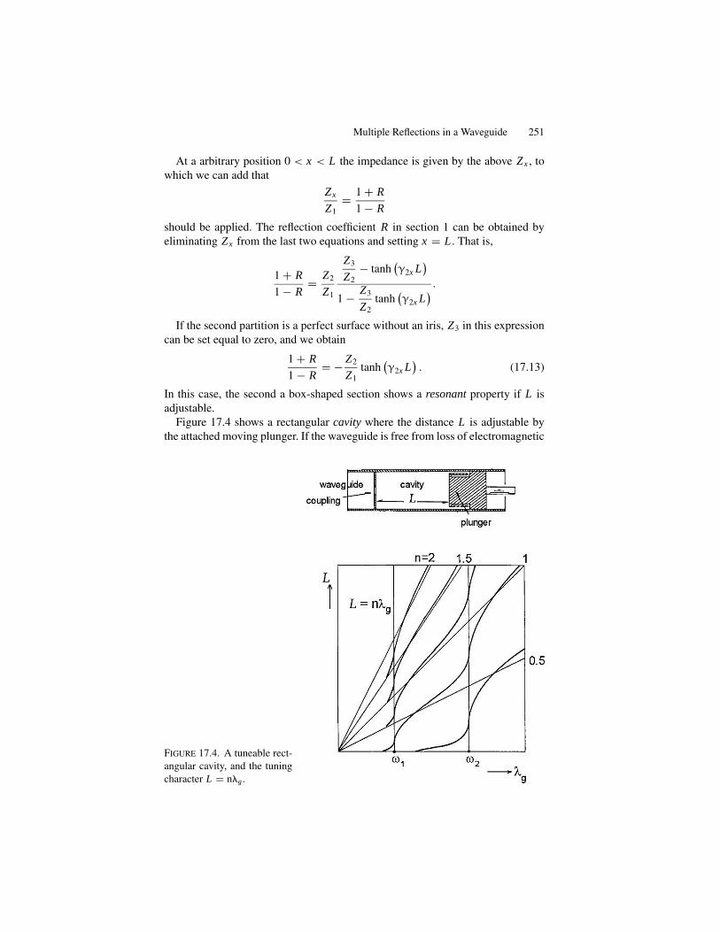
Multiple Reflections in a Waveguide 251
At a arbitrary position 0 < x < L the impedance is given by the above Zx , towhich we can add that
Zx
Z1
= 1 + R
1 − R
should be applied. The reflection coefficient R in section 1 can be obtained byeliminating Zx from the last two equations and setting x = L . That is,
1 + R
1 − R= Z2
Z1
Z3
Z2
− tanh(γ2x L
)
1 − Z3
Z2
tanh(γ2x L
) .
If the second partition is a perfect surface without an iris, Z3 in this expressioncan be set equal to zero, and we obtain
1 + R
1 − R= − Z2
Z1
tanh(γ2x L
). (17.13)
In this case, the second a box-shaped section shows a resonant property if L isadjustable.
Figure 17.4 shows a rectangular cavity where the distance L is adjustable bythe attached moving plunger. If the waveguide is free from loss of electromagnetic
FIGURE 17.4. A tuneable rect-
angular cavity, and the tuning
character L = ng .
252 17. Waveguide Transmission
energy, the constant �2x is pure imaginary, i.e., γ2x = ikx , and tanh (ikx L) =i tan(kx L). Then, from (17.13), if tan(kx L) = 0, we obtain R = 0, signifying
that there is no reflection if kx L = � × integer. Using the relation kx = 2π
g
, this
condition for resonance can be rephrased as
L = g
2× integer. (17.14)
At resonance, electromagnetic fields in such an idealized cavity reflect back andforth between two walls, resulting in stationary waves with large amplitude, asspecified by (17.14). However, a real cavity cannot be idealized as free fromenergy loss. Nevertheless, a cavity can be represented approximately by a loadedimpedance ZL = −iZ2tan(kx L) behaving as a reactance for an arbitrary L .

19Electronic Excitation ofCavity Oscillations
19.1. Electronic Admittance
A resonator is an essential device for sustained oscillations, such as a triode os-cillator, in which the oscillating current is controlled by a resonant LC load. Inmicrowave oscillators a cavity resonator controls the electronic current to sustainoscillation in the feedback mechanism. The electronic current density j can interactwith a cavity when passing through an area dominated by the E vector. Either fromelectrons traveling to the cavity or in the opposite direction, the transferred energyoperates the device like an oscillator or an electron accelerator. Sharing a similarprinciple, a betatron accelerator is operated at low frequencies for acceleratingelectrons by an alternating dynamic E field that arises from a sinusoidal magneticflux.
In the equations (18.13) and (18.14) for amplitudes of the normal mode i, theterms of d ji
/dt and ji can act as the driving force for forced oscillation if ji at
the opening area S′ interacts with the fields of the cavity mode. Since electroniccurrents are technically feasible at high intensity, such interactions can be utilizedfor a variety of applications in modern technologies, such as high-power oscillatorsand particle accelerators. We define the electronic admittance for such interactions,as discussed in the following.
A coupling between the waveguide and cavity mode was previously expressedby the electric field
E =∑
i
Eiei =∑
j
Vj Etj and Vj =∑
j
vij Ej,
together with the corresponding H given by
H =∑
j
Ij Zo Htj
at the iris. The input impedance can be defined with coefficients Vj and Ij as
Z input =∑
j
Vj
Ij
=∑
j
vij
Ij
Ej = v11
I1
E1 + Z ′,
268
Electronic Admittance 269
where
Z ′ =∑j�=1
v1j
Ij
E ′j,
and hence
I1 = v11 E1
Z input − Z ′ .
The integral for coupling on the area S′ in (18.13) and (18.14) can be written as
∫S′
(n × H).e1dS′ = I1v11 +∑j�=1
Ijv1j = I1v11 +∑j�=1
v21j E1
Z input − Z ′ ,
whereas the integral for damping on S can be expressed as
∫S
(n × E).h1dS = E1
√��o
2�(1 + j)
∫S
h21dS.
By an oscillating I1 ∝ exp(i�t), the cavity mode E1 is forced to oscillate, forwhich equation (18.13) has a steady solution
(−εo�o�2 + k21)E1
=−i��o j1 + εo I1v11 + εo E1
∑j
v21j
Z input − Z ′ − k1 E1
√��o
2�(1 + i)
∫S′
h21dS′
or [i
(�
�1
− �1
�
)+ (1 + i) �
2
∫S
h21dS + 1
εo�1
∑j�=1
v2j1
Z input − Z ′
]
× E1 + 1
εo�1
j1 = I1v11
εo�1
,
where � is the skin depth. As defined in Section 18.4, we write
�
2
∫S
h21dS = 1
Qwall
,1
Z1
∑j�=1
v21j
εo�1
Z1
Z input − Z ′ = 1
Qext
andZ1
Z input − Z ′ = g1 + ib1,
and obtain the expression
E1 =I1v11
εo�1
i
(�
�′1
− �′1
�
)+ 1
Qwall
+ g1
Qext
+ j1εo�1 E1
,

270 19. Electronic Excitation of Cavity Oscillations
where
�′1 = �1
(1 − 1
Qwall
− b1
Qext
).
Here, in the expression of E1, the last term in the denominator can be interpretedas an energy loss due to the current j1 in the electric field E1, which is thereforeexpressed as
1
Qel
=12
j1 E∗1(
12εo E1 E∗
1
)�1
. (19.1)
It is noted that this electronic Qel can be negative if the current j1 and the fieldE1 are out of phase; but Qel is positive if they are in phase. Such a negative Qel
corresponds to negative feedback in a triode oscillator at low frequencies, wherethe grid current and anode voltage are out of phase in oscillating condition. Onthe other hand, a positive Qel gives a condition for acceleration if the resonator isused as an accelerator.
Although unspecified in the above, for efficient interactions electronic currentsshould pass through a part of the cavity field where E1 is predominant with a highdensity of field-lines. Considering that such a part of E1 is signified by a highvoltage difference �V across a narrow gap d, analogous to a static case, we canwrite E1 = �V /d , and
1
Qel
∼ I1
A
d
εo�1�V= I1
C�1�V= ge + ibe
C�1
, (19.2a)
where A is the effective area for the current I1, C = εo A
dis a capacity by static
analogy, andI1
�V= ge + ibe may be called the electronic admittance. Thus, for
a cavity interacted with a current, we have the formulae
1
Q= 1
Qwall
+ g1
Qext
+ ge
Qel
(19.2b)
and
�′1 = �1
(1 − 1
Qwall
− b1
2Qext
− be
2Qel
). (19.2c)
19.2. A Klystron Cavity
In a cavity of a klystron oscillator, E-lines are distributed in high density in aparticular region, shown in Figure 19.1. The cavity is basically a short cylindricalcoaxial cavity with both ends closed, and the central conductor is a hollow cylinderwith a narrow gap of parallel grids, as illustrated in Figure 19.1(a). The field-linesof E are radial with regard to the x-axis in most parts of the coaxial space, exceptfor in the gap area, where they are almost parallel to the axis. The hollow centralcylinder is designed for electrons to pass inside through the grids, where they

A Klystron Cavity 271
FIGURE 19.1. A klystron cavity.
(a) A sectional view. (b) E-lines
near the grids.
interact with the E-field. In fact, it is not so easy to find the mathematical solutionto the Maxwell equations in such a cavity; however, the important feature of thegap is intuitively clear.
We can consider that the cavity is in a continuous coaxial structure, in which a gapin the center conductor can be considered as a perturbation. Slater discussed sucha perturbation, one that modifies the conducting boundary of the cavity, resultingin a shift of the resonance frequency. Consider that the conducting boundary S isdisplaced inward to S∗ by making a small dent on S, as illustrated in Figure 19.2. Inthis case, in a small volume v∗ between S and S∗, the field vectors E and H shouldbecome zero by displacing S to S∗, hence creating a discontinuity of the tangentialcomponent of H on S∗. Consequently, the equations of the normal oscillation areforced by an additional perturbation − ∫
S∗ (n × H).e1dS∗. Assuming H ≈ H1h1,this perturbation can be written as
−H1
∫S∗
(n × h1).e1dS∗ = −H1
∫S∗
(e1 × h1).dS∗,
FIGURE 19.2. A boundary perturbation for
Slater’s theorem.
272 19. Electronic Excitation of Cavity Oscillations
whereas ∫S
(e1 × h1).dS = 0.
Applying Gauss’s theorem to the volume v∗, we can write
H1
{∫S+S′
(e1 × h1).d(S + S′)} = H1
∫v∗
div(e1 × h1) dv∗,
where
div (e1 × h1) = h1.curl e1 − e1.curl h1 = k1
(h2
1 − e21
).
Therefore, resulting from such a perturbation the steady solution of (18.14) can beshifted as given by
−εo�o�2 + k21 = −k2
1
∫v∗
(h2
1 − e21
)dv∗,
or
�2 = �21
{1 +
∫v∗
(h2
1 − e21
)dv∗
}, where �1 = k1√εo�o
. (19.3)
As shown in Figure 19.1, between the two grids, the field is predominantly electric,so that at least qualitatively, � < �1, giving a resonant frequency lower than thenormal mode in the unperturbed cavity. In contrast, we can obtain � > �1 if weare considering a similar magnetic perturbation.
Such a frequency shift due to a capacitive perturbation can also be estimated bythe following calculation. Using cylindrical coordinates r , �, x , the unperturbedcoaxial mode at the lowest normal mode can be expressed by
Er (r, x, t) = Eo
rsin
(2�x
�− �t
)
and
H�(r, x, t) = −i
√εo
�o
Eo
rcos
(2�x
�− �t
),
representing a standing wave along the x direction. This is in fact the TEM modeof propagation, and k = 2�/�, for which we can define the voltage and currentfunctions as
V (x, t) = −∫ b
aErdr = −Eo ln
b
asin
(2�x
�− �t
)
and
I (x, t) =∮
H�rd� = −i (2�r )
√εo
�o
Eo
rcos
(2�x
�− �t
)
= −2�i
√εo
�o
Eo cos
(2�x
�− �t
).

A Klystron Cavity 273
Assuming that the grids of gap d are located exactly at the center as in the figure,we can calculate the potential difference as
�V (t) = V
(h + d
2, t
)− V
(h − d
2, t
)
≈ −2Eo lnb
asin
(�h
�− �t
), if d h.
On the other hand, the current is
I (1h, t) = −2�i
√εo
�o
Eo cos
(�h
�− �t
)
under the same condition. Therefore
1
i�C= V
(12h, t
)I(
12h, t
) = 1
�i
√�o
εo
lnb
atan
(�h
�− �t
),
from which we can define a capacity C = εo�a2
d, and write the relation
�
a=
√2�2h
dln
b
a,
justifying that � > a, if d < h. Therefore, the wavelength � for the resonance canbe increased significantly by reducing the gap d, making the cavity substantiallysmall. Such a small cavity can be easily installed in a vacuum tube of convenientsize.
Further, we can verify that such a cavity has an important feature, required foran efficient interaction with electrons. In an unperturbed coaxial cavity the fieldenergy distributed over the whole volume can be calculated as
∫cavity
E2dv = E2o
b∫a
2�rdr
r2
�∫0
sin2 2�x
�dx = �E2
o
6
(2�
�
)2
h3 lnb
a,
while the energy in the capacitive volume in the perturbed cavity can be estimatedas
∫gap
E2dv = �V(
12h)2
C= �a2 E2
o
(2�
�
)2 h2
dln
b
a.
The ratio between them can then given by
∫gap
E2dv
/∫cavity
E2dv = �2
3
(h
�
)2
,
which is large, if � h.

274 19. Electronic Excitation of Cavity Oscillations
FIGURE 19.3. (a) Two-cavity klystron. (b) Reflex klystron.
19.3. Velocity Modulation
We consider a continuous flow of electrons in one dimension from the cathode,which is described by the continuity equation of charge and current. Such a cur-rent as caused by a static voltage is primarily a steady current, as characterizedby a constant charge density, i.e., ∂
/∂t = 0, at any point in the path of elec-
trons moving at a constant density, i.e., div j = 0 at any time. If this conditionis violated, and j should be changed with respect to the continuity law, i.e.,div j + ∂
/∂t = 0, where j = vv. In a one-dimensional flow with v = constant,
we have a solution = (x − vt), expressing that all electrons are moving at thesame constant speed v.
Figure 19.3 shows a practical arrangement for such a current in a vacuum tube.Electrons emitted by the cathode are accelerated by the potential Vo between thecathode and cavity, as shown in Figure 19.3(b). Denoting the mass and charge ofan electron by m and e, respectively, we have the energy relation, i.e., 1mv2
o = eVo,which is valid before electrons enter the cavity. Needless to say, Vo must be negativeto accelerate electrons to a speed vo. Between the two grids there is a potentialdifference �V cos(�1t), where the speed changes from vo to v1 according to therelation
1 mv21 − 1 mv2
o = −e�V cos �1t,
hence we can write that
1 mv21 = e[Vo + �V cos(�1t)],
Velocity Modulation 275
or
v1 = vo
[1 − �V
2Vo
cos(�1t)
]for �V Vo. (19.4)
Thus, electrons are further accelerated or decelerated, depending on the sign ofthe potential �V cos(�1t). Owing to the periodic potential, accelerated electronscatch up with those that are slowed down after passing through the cavity, andconsequently the electron density is periodically modulated. Electrons are thussaid to be velocity modulated, resulting in so-called electron bunching. Generally,such a modulated current is rich in harmonic frequencies of �1, hence it is utilizedfor generating intense coherent radiation at �1 or other applications.
It is noted that after it is modulated at to in the cavity (called a buncher), thebunched density arrives at a position x at a later time t = to + x/v1, which can bewritten as
t = to + x
vo
√1 + �V
Vo
cos �1to
. (19.5)
Therefore, the modulated beam current can be expressed as
I (x, t) = edN
dt= e
dN
dto
dtodt
= Io
dtodt
, (19.6)
where Io = edN
dto. Here, dto/dt can be obtained from (19.6), i.e.,
dtodt
= 1
1 + sin �1to,
where the factor = 1
2
x�1
vo
�V
Vo
is called the bunching parameter. For a small
value of we also obtain the relation �1(t − x
vo
) = �1to − cos(�1to), which can
be used as the phase variable for the Fourier expansion of the current I (x, t).Considering that the electron density at x = 0 is modulated by the potential �V
in a period of time 0 ≤ to ≤ 2�/�1, we can express I (x, t) at an arbitrary point xin the drift space by the Fourier series
I = I1 +∑
n
{An cos n�1
(t − x
vo
)+ Bn sin n�1
(t − x
vo
)},
where
I1 = �1
2�
2�/�1∫0
I (x, t) dt = Io,
An = �1
�
2�/�1∫0
I (x, t) cos n�1
(t − x
vo
)dt,
276 19. Electronic Excitation of Cavity Oscillations
and
Bn = �1
�
2�/�1∫0
I (x, t) cos n�1
(t − x
vo
)dt .
We can rewrite these coefficients by using an angular variable �1t = �, that is,
An = Io
�
2�∫0
cos n (� − cos �) d�
= (−1)n/2 2Io Jn (n) for n even, 0 for n odd,
and
Bn = Io
�
2�∫0
sin n (� − cos �) d�
= (−1)12
(n−1) 2Io Jn (n) for n odd, 0 for n even,
where Jn(n) is the Bessel function in integral form.The velocity modulated current Ibunch is therefore expressed as a series of com-
ponent waves with amplitudes changing periodically as described by Bessel’sfunctions:
Ibunch = Io + 2Io J1 () sin
[�1
(t − x
vo
)]
− 2Io J2 (2) cos
[2�1
(t − x
vo
)]− 2Io J3 (3) sin
[3�1
(t − x
vo
)]
+ 2Io J4 (4) cos
[4�1
(t − x
vo
)]+ · · · . (19.7)
Figure 16.5 shows curves of some Bessel’s functions, varying periodically ascharacterized by the parameter , each of which indicates a maximum at a specificphase of propagation. Electrons and the cavity field can interact significantly ifthey are in phase at the same frequency �1. Obviously, a bunch for n =1, i.e.,
the second term 2Io J1 sin[�1
(t − x
vo
)], is the most important component among
others, interacting in phase with an oscillating field at �1. From Table 16.1, shownin Appendix, the curve of J1() is maximum at max = 1.841, where J1(max) =0.5819, giving a significantly large amplitude.
19.4. A Reflex Oscillator
Figures 19.3(a) and 19.3(b) show a schematic layout in two-cavity and reflexklystrons, respectively, which are vacuum tube devices commonly used as mi-crowave oscillators. The former is generally suitable for high-power generation,
A Reflex Oscillator 277
whereas the latter is designed as a low-power oscillator in other applications. Asshown in Figure 19.3(a), a second cavity is installed for interactions with bunchedcurrents from the first cavity, whereas in the reflex oscillator of Figure 19.3(b)the bunched current is reflected back by an additional electrode, called the re-flector, to interact with the cavity. For whichever operation—either oscillator oraccelerator—the transit time of the bunched current is essential, and it is adjustableby a negative potential difference VR applied between the two-cavity klystron in(a), and between the cavity and reflector in (b). Here, we discuss a reflex klystron,in which the reflector voltage VR is essential for selecting mode of operation.
Letting d be the distance between the cavity and the reflector and to the time fora bunch to start from the cavity, the speed should change to
v = vo − eVR
md(t − to) .
Considering that the speed is −vo when electrons are returning to the cavity, thetime t can be expressed as
t = to + 2md
eVR
v = to + 2mvod
eVR
(1 − �V
2Vo
cos �1to
).
In terms of the phase, the current phase is shifted from the starting phase �1to as
�1t = �1to + � + 1
2��V
Vo
cos �1to,
where � = �1
2mvod
eVR
signifies a phase difference arising from the transit process,
and in the last term � = 1
2��V
Vo
represents the bunching effect, similar to the
parameter . It is noted, however, that the parameter �, as related to �, is notidentical to .
When returned from the reflector to x = 0, the phase of the reflected electronbunch is considered as �1t − � = �1to − �cos�1to. Therefore, by the Fourier ex-pansion, the reflected current Iref(t) can be expressed as
Iref(t) = I1 +∑
n
{An cos [n (�1t − �)] + Bn sin [n (�1t − �)]},
we have
I1 = Io, An = �1
2�
2�/�1∫0
Iref (t) cos [n (�1t − �)] dt
= Io
�
2�∫o
cos [n (� − � cos �)] d�
278 19. Electronic Excitation of Cavity Oscillations
and
Bn = �1
�
2�/�1∫0
Iref (t) sin [n (�1t − �)] dt = Io
�
2�∫0
sin [n (� − � cos �)] d�,
where the variable � = �1to is considered a continuous variable in the range 0 ≤� ≤ 2�. For bunching, we have already discussed that the last integrals in theabove are Bessel’s functions of the nth order, i.e.,
An = (−1)n/2 2Io Jn (n�) for n even
and
Bn = (−1)n+1/2 2Io Jn (n�) for n odd.
Therefore, the reflected current at x = 0 can be expressed as
Iref(t) = Io − 2Io J1(�) sin(�1t − �) + 2Io J2(2�)cos2(�1t − �) + · · · . (19.8)
Forareflexklystron,weareonlyinterestedinthecomponent2Io J1(�)sin(�1t−�)against the voltage �V cos(�1t) across the grids. Due to the interaction energyj .E, the negative sign is required for sustaining oscillation in the cavity, for whichthe phase difference � plays an essential role. In fact, such an oscillatory conditioncan be met at any angle of � − (3�/2) × m, where m is an integer, which can beachieved by adjusting the reflector voltage VR, since � is defined as it relates toVR. In a practical reflex klystron the oscillator power exhibits a series of peaks asVR is varied.
Using complex forms for this particular component of Iref(t) and grid voltage�V , we can write the electronic admittance as
ge + ibe = 2Io J1 (�) exp{i(�1t − � + 3�
2
)}�V exp {i (�1t)} ,
where �V = 2�Vo
�by definition. Accordingly, we have
ge + ibe = Io
Vo
� exp
{−i
(� − 3�
2
)}J1 (�)
�,
and these, the electronic conductance and susceptance, are related as
be
ge
= − tan
(� − 3�
2
).
The power for exciting the cavity field can then be expressed as
Pe = −2Io J1 (�) cos
(� − 3�
2
)× 2�Vo
�= −1
2geV 2
o �J1(�)

A Reflex Oscillator 279
FIGURE 19.4. Bessel’s function
J1(�), and J1(�)/�, �J1(�) vs. �.
where
ge = − Io
Vo
� cos
(� − 3�
2
)J1 (�)
�,
which is directly related to the reflector voltage VR, expressed as
VR ∝ 1
�cos
(� − 3�
2m
).
where m is an integer. Figure 19.4 shows sketches of J1(�), J1(�)/� and �J1(�)as functions of �, which can be used for evaluating the oscillation spectrum andintensities.

18Resonant Cavities
18.1. Slater’s Theory of Normal Modes
In Section 17.3, we discussed the property of a resonant cavity in a rectangu-lar TE mode. Primarily, it is a matter of analytical convenience, but in principleresonance can be found at a given frequency for a cavity of arbitrary shape. Inthis chapter, following Slater, we discuss resonant properties of a cavity of gen-eral shape, for which the Maxwell equations can provide oscillating modes withintense amplitudes (J. C. Slater, Microwave Electronics, Van Nostrand, 1950.)
Electromagnetic waves from an oscillator are transmitted through the waveguideto a cavity connected at the end. In this case the energy in the cavity exhibits aresonance behavior at a particular frequency �i. Slater showed that the amplitudesof field vectors E and H inside a cavity are oscillatory and described in terms ofthe normal mode function at a frequency �i. The oscillator frequency � shouldtherefore be equal to �i of a normal mode, i.e., � = �i, which is the conditionrequired for resonance at which the field vectors are expressed in terms of thenormal mode i.
We pay attention to the fact that any vector field consists of solenoidal andirrotational components signified as free from divergence (div) and rotation (curl),respectively. For such electromagnetic fields we should obtain two solenoidalfunctions ei and hi to express the solenoidal part of E and the fully solenoidal H,while we need an irrotational function e′
i for the irrotational part of E. To expressthese E and H expanded with regard to these mode functions the orthogonalityrelations should be established among mode functions ei, hi and e′
i.Owing to the relations div ei = 0 and div hi = 0, solenoidal vectors ei and hi
can be expressed by curls of hi and ei, respectively. We therefore assume that
kiei = curl hi and kihi = curl ei, (18.1)
where ki is a constant. Then, using the vector identity relation, curl(curl) =grad(div) −�, we can obtain the wave equations characterized by the same ki
for these solenoidal vectors ei and hi, i.e.,(� + k2
i
)(ei, hi) = 0, (18.2)
253
254 18. Resonant Cavities
indicating that these ei and hi can constitute a normal mode i specified by theconstant ki.
Further, using the relations in (17.1) we can show that ei and hi can satisfy theboundary conditions on the conducting walls S and opening areas S′ of a cavity ifthe field vectors E and H can be represented by these mode vectors. Denoting theunit vector normal to inner surfaces by n, we obtain
n × ei = 0 on S and n × hi = 0 on S′, (18.3a)
by applying Stokes’ theorem to (18.1). Also, applying Gauss’s theorem we canshow that the normal components are continuous, i.e.,
n.hi = 0 on S and n.ei = 0 on S′. (18.3b)
Using these boundary conditions, next we can obtain orthogonality relations ofthese normal modes. For that purpose we use the identity relation
div(ej × curl ei) − div(ei × curl ej) = curl ei.curl ej − ej.curl(curl ei)
− curl ej.curl ei + ej.curl(curl ei),
where the left side can be simplified as(
k2j − k2
i
)ei.ej by (18.2). Applying the
Gauss theorem to the above expression in the cavity volume v, converting then tothe surface integral over S + S′, we obtain∫
S,S′
n.(ej × kihi − ei × kjhj)d(S, S′) = (k2j − k2
i )∫v
ei.ej dv (i)
The surface integrals on the left side can be written as∫S
{kihi.(n × ej
) − kjhj.(n × ei)} dS +∫S′
{kjei.(n × hj) − kiej.(n × hi)} dS′
where all terms vanish on surfaces S and S′ owing to the boundary conditions(18.3a). Hence, the volume integral in (i) vanishes for ki �= kj, that is,∫
v
ei.ejdv = 0 for i �= j.
In addition, we consider that these ei are normalized to 1, i.e.,∫v
e2i dv for i = j,
and hence the orthonormal condition for the vector ei is expressed as∫v
ei.ej dv = �ij, (18.4a)
where �ij = 1 if i = j, otherwise 0 for all i �= j, and is known as the Kroneckerdelta.
The orthogonalty for the vector hi can be verified in a manner similar to ei.In fact, hi and ei are related by (18.1), therefore if ei is normalized, hi is also
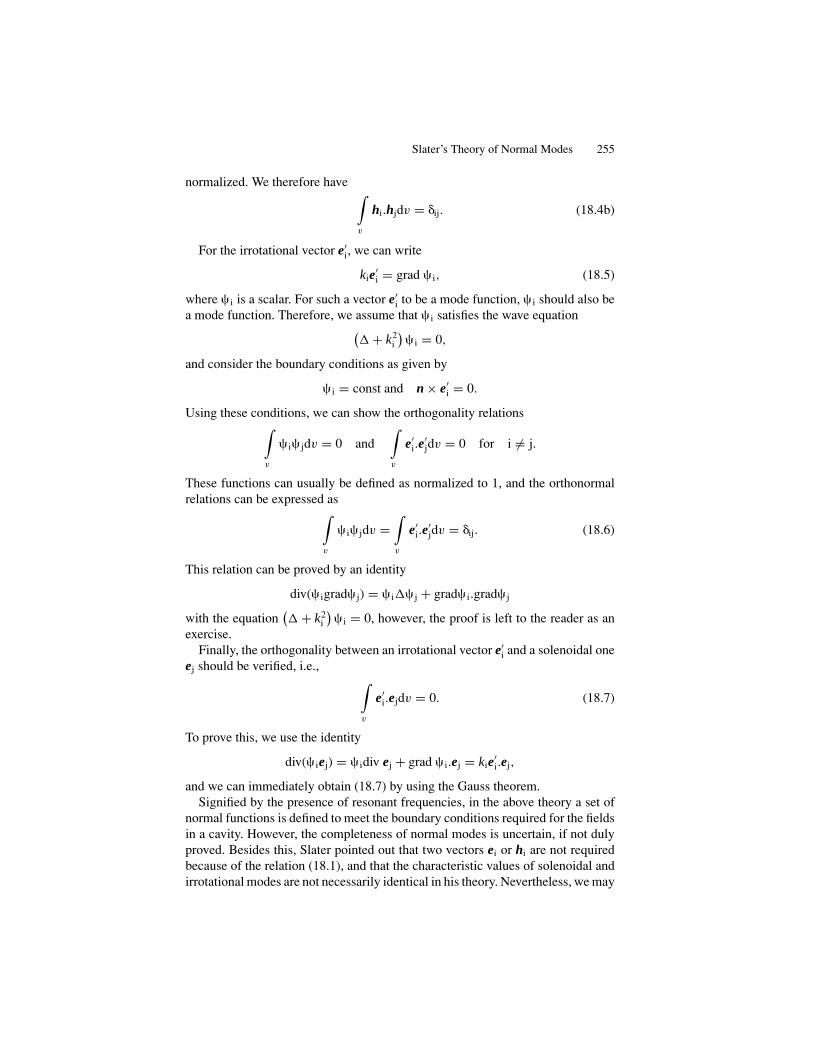
Slater’s Theory of Normal Modes 255
normalized. We therefore have ∫v
hi.hjdv = �ij. (18.4b)
For the irrotational vector e′i, we can write
kie′i = grad � i, (18.5)
where � i is a scalar. For such a vector e′i to be a mode function, � i should also be
a mode function. Therefore, we assume that � i satisfies the wave equation(� + k2
i
)� i = 0,
and consider the boundary conditions as given by
� i = const and n × e′i = 0.
Using these conditions, we can show the orthogonality relations∫v
� i� jdv = 0 and∫v
e′i.e
′jdv = 0 for i �= j.
These functions can usually be defined as normalized to 1, and the orthonormalrelations can be expressed as∫
v
� i� jdv =∫v
e′i.e
′jdv = �ij. (18.6)
This relation can be proved by an identity
div(� igrad� j) = � i�� j + grad� i.grad� j
with the equation(� + k2
i
)� i = 0, however, the proof is left to the reader as an
exercise.Finally, the orthogonality between an irrotational vector e′
i and a solenoidal oneej should be verified, i.e., ∫
v
e′i.ejdv = 0. (18.7)
To prove this, we use the identity
div(� iej) = � idiv ej + grad � i.ej = kie′i.ej,
and we can immediately obtain (18.7) by using the Gauss theorem.Signified by the presence of resonant frequencies, in the above theory a set of
normal functions is defined to meet the boundary conditions required for the fieldsin a cavity. However, the completeness of normal modes is uncertain, if not dulyproved. Besides this, Slater pointed out that two vectors ei or hi are not requiredbecause of the relation (18.1), and that the characteristic values of solenoidal andirrotational modes are not necessarily identical in his theory. Nevertheless, we may

256 18. Resonant Cavities
consider that these mode functions (ei, hi, e′i, and � i) are sufficiently adequate to
express the electromagnetic field Ei, Hi, and associated quantities at resonance.
18.2. The Maxwell Equations in a Cavity
We consider electromagnetic fields in a cavity, where the field vectors E and Hand the source j and � are all expanded into series with respect to normal modesei , hi, e′
i, and � i. We therefore write that
E =∑
i
(Eiei + E ′
ie′i
), where Ei =
∫v
E.eidv and E ′i =
∫v
E.e′idv;
H =∑
i
Hihi, where Hi =∫v
H.hidv;
j =∑
i
(jiei + j ′
i e′i
), where ji =
∫v
j .eidv and j ′i =
∫v
j .e′idv;
� =∑
i
�i� i, where �i =∫v
�� idv. (18.8)
On the other hand, we expand curl E with respect to hi for mathematical conve-nience, that is,
curl E =∑
i
hi
∫v
(curl E).hidv,
to which we apply the identity relation
div(E × curl ei) = (curl E).(curl ei) − E.(curlcurl ei)
= kihi.(curl E) − k2i E.ei,
and obtain∫v
(curl E).hidv = ki
∫v
E.eidv + 1
ki
∫v
div (E × curl ei) dv.
= ki
∫v
E.eidv +∫
S,S′
n.(E × hi)d(S, S′).
The second surface integration on the right can be performed separately on S andS′ as
∫S
hi.(n × E)dS′ + ∫S′
E.(hi × n)dS′; however the boundary condition (18.3a)
on S′ makes the second integral zero. Therefore, curl E can be expanded as
curl E =∑
i
hi
[ki Ei +
∫S
(n × E).hidS
]. (18.9a)
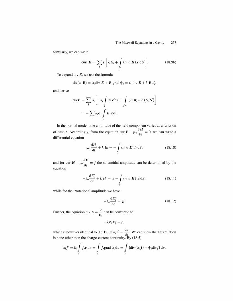
The Maxwell Equations in a Cavity 257
Similarly, we can write
curl H =∑
i
ei
[ki Hi +
∫S′
(n × H).eidS′]. (18.9b)
To expand div E, we use the formula
div(� i E) = � idiv E + E.grad � i = � idiv E + ki E.e′i,
and derive
divE =∑
i
� i
[−ki
∫v
E.e′idv +
∫S,S′
(E.n) � id(S, S′)]
= −∑
i
ki� i
∫v
E.e′idv.
In the normal mode i, the amplitude of the field component varies as a function
of time t . Accordingly, from the equation curlE + �o∂ H∂t
= 0, we can write a
differential equation
�odHi
dt+ ki Ei = −
∫S
(n × E).hidS, (18.10)
and for curlH − εo∂ E∂t
= j the solenoidal amplitude can be determined by the
equation
−εodE ′
i
dt+ ki Hi = ji −
∫S′
(n × H) .eidS′, (18.11)
while for the irrotational amplitude we have
−εodE ′
i
dt= j ′
i . (18.12)
Further, the equation div E = �
εocan be converted to
−kiεo E ′i = �i,
which is however identical to (18.12), if ki j ′i = d�i
dt. We can show that this relation
is none other than the charge-current continuity. By (18.5),
ki j ′i = ki
∫v
j .e′idv =
∫v
j .grad � idv =∫v
{div (� i j) − � idiv j} dv,
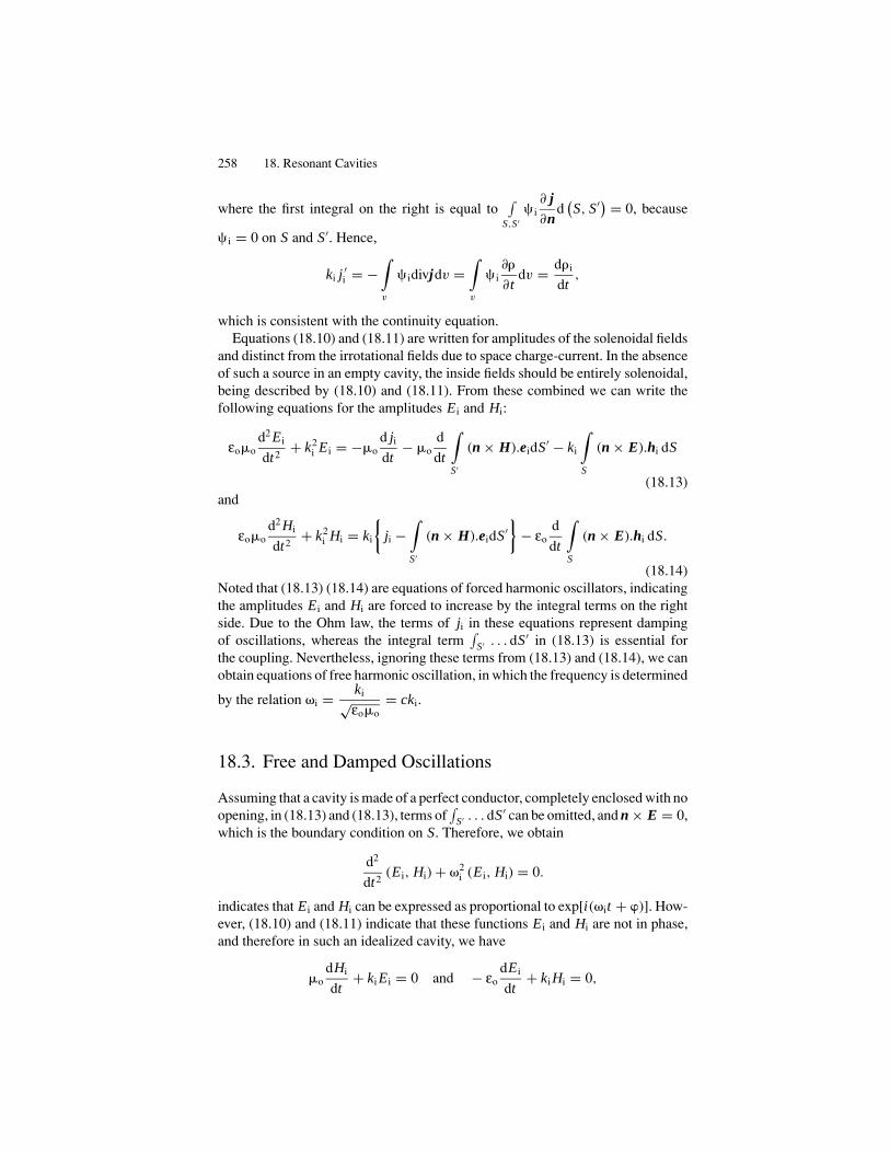
258 18. Resonant Cavities
where the first integral on the right is equal to∫
S,S′� i
∂ j∂n
d(S, S′) = 0, because
� i = 0 on S and S′. Hence,
ki j ′i = −
∫v
� idivjdv =∫v
� i∂�
∂tdv = d�i
dt,
which is consistent with the continuity equation.Equations (18.10) and (18.11) are written for amplitudes of the solenoidal fields
and distinct from the irrotational fields due to space charge-current. In the absenceof such a source in an empty cavity, the inside fields should be entirely solenoidal,being described by (18.10) and (18.11). From these combined we can write thefollowing equations for the amplitudes Ei and Hi:
εo�od2 Ei
dt2+ k2
i Ei = −�od jidt
− �od
dt
∫S′
(n × H).eidS′ − ki
∫S
(n × E).hi dS
(18.13)and
εo�od2 Hi
dt2+ k2
i Hi = ki
{ji −
∫S′
(n × H).eidS′}
− εod
dt
∫S
(n × E).hi dS.
(18.14)Noted that (18.13) (18.14) are equations of forced harmonic oscillators, indicatingthe amplitudes Ei and Hi are forced to increase by the integral terms on the rightside. Due to the Ohm law, the terms of ji in these equations represent dampingof oscillations, whereas the integral term
∫S′ . . . dS′ in (18.13) is essential for
the coupling. Nevertheless, ignoring these terms from (18.13) and (18.14), we canobtain equations of free harmonic oscillation, in which the frequency is determined
by the relation �i = ki√εo�o= cki.
18.3. Free and Damped Oscillations
Assuming that a cavity is made of a perfect conductor, completely enclosed with noopening, in (18.13) and (18.13), terms of
∫S′ . . . dS′ can be omitted, and n × E = 0,
which is the boundary condition on S. Therefore, we obtain
d2
dt2(Ei, Hi) + �2
i (Ei, Hi) = 0.
indicates that Ei and Hi can be expressed as proportional to exp[i(�it + �)]. How-ever, (18.10) and (18.11) indicate that these functions Ei and Hi are not in phase,and therefore in such an idealized cavity, we have
�odHi
dt+ ki Ei = 0 and − εo
dEi
dt+ ki Hi = 0,
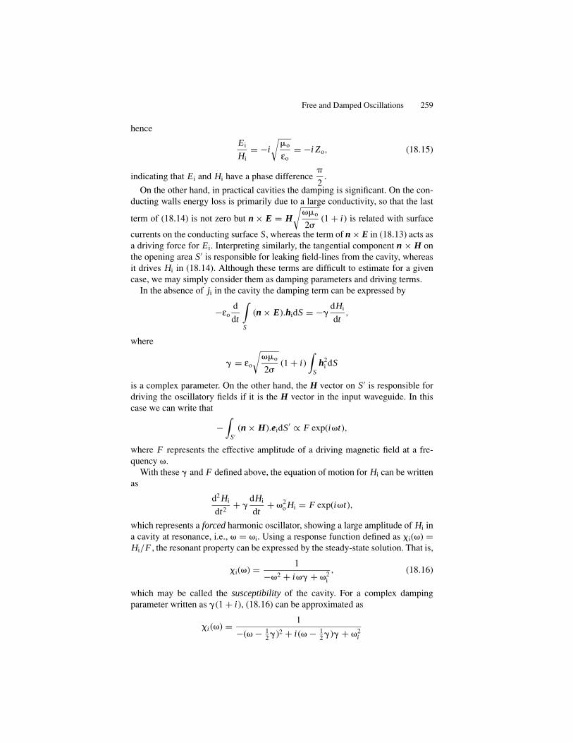
Free and Damped Oscillations 259
hence
Ei
Hi= −i
√�o
εo= −i Zo, (18.15)
indicating that Ei and Hi have a phase difference�
2.
On the other hand, in practical cavities the damping is significant. On the con-ducting walls energy loss is primarily due to a large conductivity, so that the last
term of (18.14) is not zero but n × E = H√
��o
2(1 + i) is related with surface
currents on the conducting surface S, whereas the term of n × E in (18.13) acts asa driving force for Ei. Interpreting similarly, the tangential component n × H onthe opening area S′ is responsible for leaking field-lines from the cavity, whereasit drives Hi in (18.14). Although these terms are difficult to estimate for a givencase, we may simply consider them as damping parameters and driving terms.
In the absence of ji in the cavity the damping term can be expressed by
−εod
dt
∫S
(n × E).hidS = −dHi
dt,
where
= εo
√��o
2(1 + i)
∫S
h2i dS
is a complex parameter. On the other hand, the H vector on S′ is responsible fordriving the oscillatory fields if it is the H vector in the input waveguide. In thiscase we can write that
−∫
S′(n × H).eidS′ ∝ F exp(i�t),
where F represents the effective amplitude of a driving magnetic field at a fre-quency �.
With these and F defined above, the equation of motion for Hi can be writtenas
d2 Hi
dt2+
dHi
dt+ �2
o Hi = F exp(i�t),
which represents a forced harmonic oscillator, showing a large amplitude of Hi ina cavity at resonance, i.e., � = �i. Using a response function defined as �i(�) =Hi/F , the resonant property can be expressed by the steady-state solution. That is,
�i(�) = 1
−�2 + i� + �2i
, (18.16)
which may be called the susceptibility of the cavity. For a complex dampingparameter written as (1 + i), (18.16) can be approximated as
�i (�) = 1
−(� − 12 )2 + i(� − 1
2 ) + �2i
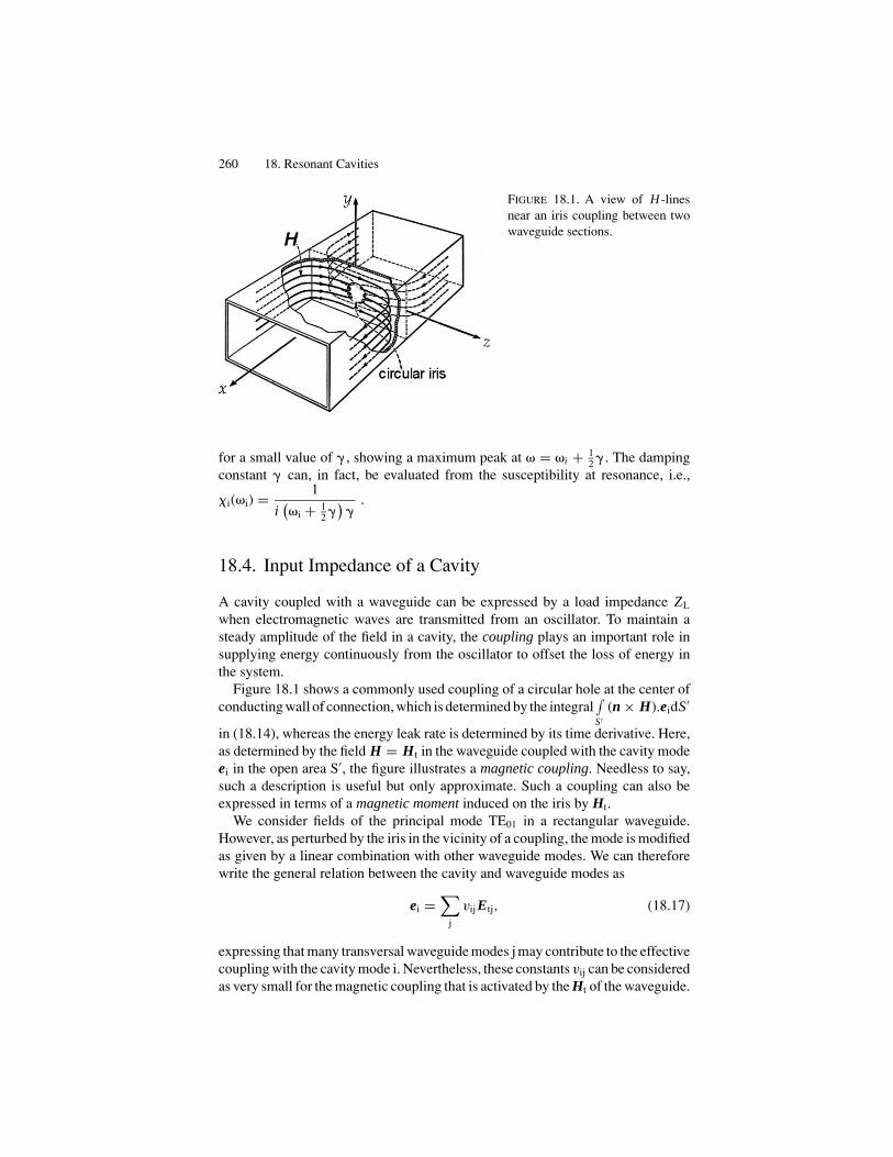
260 18. Resonant Cavities
FIGURE 18.1. A view of H -linesnear an iris coupling between twowaveguide sections.
for a small value of , showing a maximum peak at � = �i + 12 . The damping
constant can, in fact, be evaluated from the susceptibility at resonance, i.e.,
�i(�i) = 1
i(�i + 1
2 )
.
18.4. Input Impedance of a Cavity
A cavity coupled with a waveguide can be expressed by a load impedance ZL
when electromagnetic waves are transmitted from an oscillator. To maintain asteady amplitude of the field in a cavity, the coupling plays an important role insupplying energy continuously from the oscillator to offset the loss of energy inthe system.
Figure 18.1 shows a commonly used coupling of a circular hole at the center ofconducting wall of connection, which is determined by the integral
∫S′
(n × H).eidS′
in (18.14), whereas the energy leak rate is determined by its time derivative. Here,as determined by the field H = Ht in the waveguide coupled with the cavity modeei in the open area S′, the figure illustrates a magnetic coupling. Needless to say,such a description is useful but only approximate. Such a coupling can also beexpressed in terms of a magnetic moment induced on the iris by Ht.
We consider fields of the principal mode TE01 in a rectangular waveguide.However, as perturbed by the iris in the vicinity of a coupling, the mode is modifiedas given by a linear combination with other waveguide modes. We can thereforewrite the general relation between the cavity and waveguide modes as
ei =∑
j
vij Etj, (18.17)
expressing that many transversal waveguide modes j may contribute to the effectivecoupling with the cavity mode i. Nevertheless, these constants vij can be consideredas very small for the magnetic coupling that is activated by the Ht of the waveguide.

Input Impedance of a Cavity 261
In this case, we also write
H =∑
j
Ij Zo Htj, (18.18)
where Ij represents the amplitude of a TEj mode, for which the wave impedanceshould be written as Z j = Zo(k/kx ) if Ij implies a current, but in this case the factork/kx is included in the definition of Ij . For the coupling, n × H can be expressedas
n × H =∑
j
Ij Zo(n × Htj
) =∑
j
Ij Etj,
so that ∫S′
(n × H).eidS′ =∑
j
Ijvij.
Then, the steady solution for Ei can be obtained from the oscillator equation(18.13), by considering Ij ∝ exp(i�t), that is,
Ei =∑
j
Ijvij
iεo�i
(�
�i− �i
�
)−1
if damping on S is neglected.Corresponding to the H vector in (18.18), the E vector in the waveguide is
written as
E =∑
j
Vj Etj,
where Vj is the amplitude of the j mode.On the other hand, owing to the continuity of n × E on S′, this waveguide field
etj should be equal to E = ∑i
Eiei inside the cavity. Hence, using (18.17),
E =∑
i
(∑j
vij Etj
)Ei.
Accordingly, we can write the relation
Vj =∑
i
Ii Z ij, where Z ij = v2ij
iεo�i
(�
�i− �i
�
)−1
. (18.19a)
The power flow to the cavity can then be expressed as
1
2
∫S′
i.(E × H∗) dS′ = 1
2
∑j
Vj I∗j Zo
∫S′
i.(
Etj × H∗tj
)dS′ = 1
2
∑j
Vj I∗j .
By analogy, the transversal Et and Ht can be regarded as voltage and current, andZ ij represents impedances between waveguide and cavity modes.
262 18. Resonant Cavities
If the cavity mode i = 1 is well isolated from the other, (18.19a) can be simplifiedfor the waveguide at j = 1, e.g., TE01 as
V1 = I1 Z11, where Z11 = v211
iεo�1
(�
�1− �1
�
)−1
+ Z ′11, (18.19b)
where Z ′11 represents small contributions from other terms than the principal mode
i = 1. Although small in magnitude, such a Z ′11 is significant for the cavity cou-
pling, and we can rewrite the above as
i
(�
�1− �1
�
)= v2
11
εo�1
1
Z11 − Z ′11
.
Further, denoting the characteristic wave impedance of TE01 mode byZ1(= k Zo/kx ), we define the coupling of the cavity with TE01 mode as
1
Qext,1= v2
11
εo�1 Z1, (18.20)
and write
Z1
Z11 − Z ′11
= g + ib. (18.21)
With these notations, we can express
i
(�
�1− �1
�+ b
Qext,1
)+ g
Qext,1= 0,
from which we obtain the relations
Z11
Z1=
1
Qext,1
i
(�
�′1
− �′1
�
)+ g
Qext,1
, where �′1 = �1
(1 − b
2Qext,1
). (18.22)
Here, the factor Qext,1 defined by (18.20) signifies the ratio between energystored in the cavity vs. energy loss due to the opening area in this case per cycleof oscillation. It is realized that the stored energy in a cavity is limited not onlyby a finite conductivity on the wall, but also by leaking through the opening.Hence, these mechanisms should be combined for the description of resonanceperformance.
Now that the oscillatory cavity fields can be described by equations of forced os-cillation (18.13) and (18.14), the cavity resonance can be discussed on the analogyof LCR circuits. We can convert the damping constant to a loss factor denotedas Qwall. We define
Qwall = �′i
stored energy
conductung loss= 2�′
i
or
1
Qwall= �
2
∫S
h2i dS,
Example of a Resonant Cavity 263
where �g =√
2/
�i�o is the skin depth. Combining the damping effect with theloss factor due to an iris (18.20), we can express the total Q-factor as
1
Q= 1
Qwall+ g
Qext,1, (18.23a)
and (18.21) can be revised as
Z11
Z1=
1
Qext,1
i
(�
�′1
− �′1
�
)+ 1
Q
, where �′1 = �1
(1 − 1
Qwall− b
2Qext,1
).
(18.23b)
In the above the coupling is represented by the reduced admittance g + ib, whileeffects of non-resonant modes are packaged into the parameter Z ′
11. Calculationsof these parameters are complicated and therefore left for empirical evaluation.We consider that the equations (18.22a) and (18.22b) are sufficient for analyzing acavity as a circuit element. As indicated by (18.22b), the characteristic frequency�′
1 shifts from the idealized case, although close to �1, and the input admittanceg + ib is adjustable in a practical circuit. The impedance Z11 is called the inputimpedance of a cavity when the transmission line is loaded in TE01 mode.
18.5. Example of a Resonant Cavity
By analogy with an acoustic resonator, we say that a cavity can be electromagneti-cally tuned when the applied frequency � is adjusted to be equal to the characteristicfrequency �1 of a cavity. Such electromagnetic resonators are not only significantin high frequency circuits, but also inside fields are large in amplitude and hencea useful device for applications where the intensity matters.
In practice the resonant condition � = �i can be achieved either by a mechanicaltuning of a cavity or by a scanning frequency of the oscillator. Here, we discussa cavity of rectangular TE01 mode again as an example of the impedance formula(18.22). Figure 18.2 shows such a cavity that can be tuned by adjusting the distanceL . In the previous discussion, we showed that if there is no reflection, the impedanceof the cavity is given by
Z11 = −i Z1 tan2�L
�g, (18.24)
where �g = �1
2�cis related with �g = �
2�cas determined by
1
�2g
= 1
�2+ 1
�2c
,
and Z1 = �g Zo
�is the constant modified for TE01 mode.

264 18. Resonant Cavities
FIGURE 18.2. (a) The tuning charac-ter in terms of the cavity impedanceR + iX in the vicinity of a resonance�P. (b) The resonance monitored bySWR . = P at resonance, and = ′ off resonance.
If the energy loss can be totally ignored the impedance Z11 is equal to thatdescribed by (18.22), and hence we write
tan
(2�L
�g
)=
1
Qext,1
�
�′1
− �′1
�
or
L = �g
2�tan−1
1
Qext,1
�
�′1
− �′1
�
+ �g
2n,
where n is an integer. The frequency shift occurs as �′1 = �1 ± �� by a small
��, and hence
�
�′ − �′1
�≈ ∓2��
�1,
approximately. Corresponding to such small ��, an angle can be defined by therelation
tan(
12 � ±
) = ± �1
2Qext,1��,

Measurements of a Cavity Resonance 265
thereby writing
L = �g
2
(n ±
�
), where = 2Qext,1� (ln �) , (18.25)
anddL
d�g= n
2+ Qext,1
�
d (ln �)
d(ln �g
) = n
2+ Qext,1
�
vg
c.
In Figure 17.4, shown are curves for L vs. �g sketched primarily as straight linesL = 1
2 �g × n, which, however, shift at resonances by increasing n by 1. Suchtransitions are shown in the figure by smooth deviations by ± /�, which are alsocontributed by Qwall in practical cases. For illustration, only two resonances aremarked, �1 and �2 in the figure.
18.6. Measurements of a Cavity Resonance
In usual practice an Et vector can be monitored by means of a small antennaattached to a semi-conductor diode, which acts as a detector. A cavity resonancecan be detected by measuring the reflection, which is signified by the impedance.
The input to a cavity can generally be expressed by the impedance formula:
Z (�)
Zg=
1
Qext,1
i
(�
�1− �1
�
)+ 1
Q
+ Z ′
Zg, (18.26)
where �1, Q, and Qext,1 are the resonant frequency, the overall quality factor, andthe coupling of the cavity, respectively; Zg is the effective wave impedance ofthe connecting waveguide. Here, the additional term of Z ′ represents contributionfrom all other modes other than the principal mode 1. At resonance � = �1, weobtain from (18.26)
Z (�1)
Zg= Q
Qext,1+ Z ′
Zg. (18.27)
Ignoring Z ′, Z (�1)/Zg can be larger or smaller than 1, depending on Q > Qext,1
or Q < Qext,1. These cases are called overcoupled or undercoupled, respec-tively, referring to the standing wave measurements, where VSWR = Vmax/Vmin =|Z (�1)|/Zg at resonance. Denoting VSWR as , (18.27) can be expressed as
= Q
Qext,1+ ′,
where = Z (�1)/
Zg and ′ = Z ′/Zg are VSWR on- and off resonance, respec-tively. Writing further that
� = Qext,1
(�
�1− �1
�
)∼ 2Qext,1
� − �1
�1(18.28a)
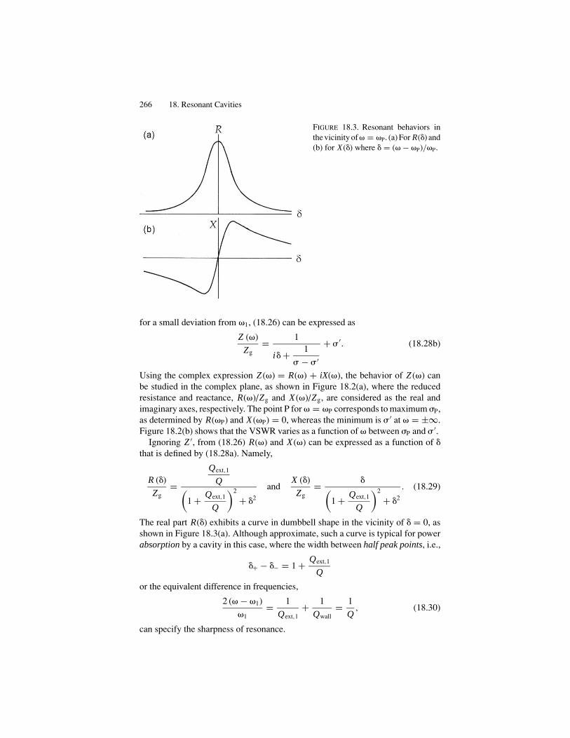
266 18. Resonant Cavities
FIGURE 18.3. Resonant behaviors inthe vicinity of � = �P. (a) For R(�) and(b) for X (�) where � = (� − �P)/�P.
for a small deviation from �1, (18.26) can be expressed as
Z (�)
Zg= 1
i� + 1
− ′
+ ′. (18.28b)
Using the complex expression Z (�) = R(�) + iX(�), the behavior of Z (�) canbe studied in the complex plane, as shown in Figure 18.2(a), where the reducedresistance and reactance, R(�)/Zg and X (�)/Zg, are considered as the real andimaginary axes, respectively. The point P for � = �P corresponds to maximum P,as determined by R(�P) and X (�P) = 0, whereas the minimum is ′ at � = ±∞.Figure 18.2(b) shows that the VSWR varies as a function of � between P and ′.
Ignoring Z ′, from (18.26) R(�) and X (�) can be expressed as a function of �that is defined by (18.28a). Namely,
R (�)
Zg=
Qext,1
Q(1 + Qext,1
Q
)2
+ �2
andX (�)
Zg= �(
1 + Qext,1
Q
)2
+ �2
. (18.29)
The real part R(�) exhibits a curve in dumbbell shape in the vicinity of � = 0, asshown in Figure 18.3(a). Although approximate, such a curve is typical for powerabsorption by a cavity in this case, where the width between half peak points, i.e.,
�+ − �− = 1 + Qext,1
Q
or the equivalent difference in frequencies,
2 (� − �1)
�1= 1
Qext,1+ 1
Qwall= 1
Q, (18.30)
can specify the sharpness of resonance.
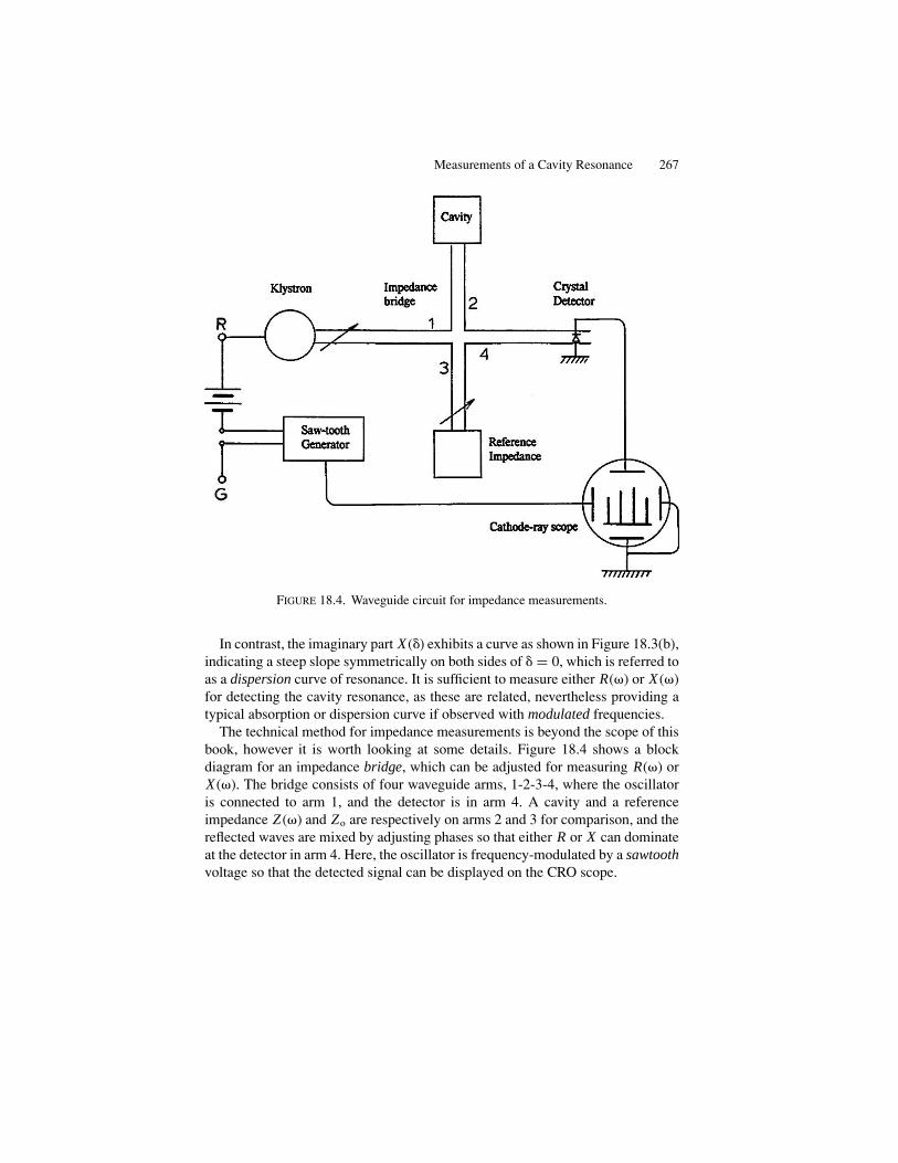
Measurements of a Cavity Resonance 267
FIGURE 18.4. Waveguide circuit for impedance measurements.
In contrast, the imaginary part X (�) exhibits a curve as shown in Figure 18.3(b),indicating a steep slope symmetrically on both sides of � = 0, which is referred toas a dispersion curve of resonance. It is sufficient to measure either R(�) or X (�)for detecting the cavity resonance, as these are related, nevertheless providing atypical absorption or dispersion curve if observed with modulated frequencies.
The technical method for impedance measurements is beyond the scope of thisbook, however it is worth looking at some details. Figure 18.4 shows a blockdiagram for an impedance bridge, which can be adjusted for measuring R(�) orX (�). The bridge consists of four waveguide arms, 1-2-3-4, where the oscillatoris connected to arm 1, and the detector is in arm 4. A cavity and a referenceimpedance Z (�) and Zo are respectively on arms 2 and 3 for comparison, and thereflected waves are mixed by adjusting phases so that either R or X can dominateat the detector in arm 4. Here, the oscillator is frequency-modulated by a sawtoothvoltage so that the detected signal can be displayed on the CRO scope.
20Dielectric and Magnetic Responses inResonant Electromagnetic Fields
20.1. Introduction
Regarding conducting properties, materials were traditionally classified into cat-egories of “conductor” or “insulator.” Today, many types of semi-conductorsas well as magnetic materials are used for a variety of applications. Mod-ern materials can be discussed properly with respect to structure, but such adiscussion is beyond the scope of this book. Nevertheless, modern empiricalknowledge of electronic charge and spin, among other properties, must be takenfor granted in order to understand classical electromagnetic theory. In addi-tion, the presence of electric and magnetic moments in constituent species isempirical.
We consider that these moments are located in solid insulating materials, ignor-ing their interactions. With this assumption, the moments can interact primarilywith applied electric or magnetic field. Macroscopically, such a response to anapplied field can be interpreted as arising from the macroscopic moment. Refer-ring to as the linear response, it is meaningful only in the limit of weak appliedfield. It is primarily an adiabatic process, but necessarily involved in a thermalrelaxation process. In practice, the response from an individual moment is tooweak to detect with conventional instruments. For example, the dipole momentof a NH3 molecule is of the order of 0.5 × 10⁻²⁹ C-m, and therefore a group ofa sufficiently large number of identical moments is required for dealing with themolecular dipole. On the other hand, in most condensed states such a responsecan be measured through the use of standing electromagnetic waves of a sizableintensity at a wavelength longer than the material size, where the field is regardedas uniform over the sample. We therefore require an LC circuit resonator at lowfrequencies or a cavity resonator at higher frequencies for response experiments,where the field has sufficiently large amplitude to interact with a group of identicalmoments. We can study the time-dependence of microscopic dipoles under suchcircumstances.
280
The Kramers–Kronig Formula 281
20.2. The Kramers–Kronig Formula
We consider a system of microscopic dipole moments embedded in a material thatis assumed as isotropic and non-conducting. For a response from the system ofdipoles to a standing wave of a time-dependent field, microscopic moments p(t)are considered as flexible and rotatable at their locations, but not as migratory inmotion. Hence, the applied field X (t) can be assumed only as a function of time,and expressed by a Fourier integral
X (t) = 1
2�
+∞∫−∞
X (�) exp(i�t) d�,
where
X (�) =+∞∫
−∞X (t) exp (−i�t) dt
is the Fourier amplitude of X (t). Considering that a moment p(t) is driven by sucha field X (t), the response function � (�) can be defined from the relation
p (t) = 1
2�
+∞∫−∞
� (�) X (�) exp (i�t) d�. (20.1a)
Assuming that X (t) = Xo�(t), where the delta function �(t) = 1 only if t = 0,otherwise zero at all t �= 0, we can interpret that the field X (�) = Xo� (�) = Xo
is switched on at t = 0 for infinitely short duration. Writing p(t)/Xo = �(t) forsimplicity, (20.1a) can be expressed as
� (t) = 1
2�
+∞∫−∞
� (�) exp (i�t) d�, (20.1b)
where �(t) is the Fourier transform of the response function � (�). Writing the func-tion in a complex form, i.e., � (�) = � ′(�) − i� ′′(�), (20.1b) can be re-expressedas
� (t) = 1
2�
+∞∫−∞
[� ′ (�) cos(�t) + � ′′ (�) sin(�t)
]d�
+ i
2�
+∞∫−∞
[� ′ (�) sin(�t) − � ′′ (�) cos(�t)
]d�.
282 20. Dielectric and Magnetic Responses in Resonant Electromagnetic Fields
For a real �(t) the integral of the second term should vanish, so that
+∞∫−∞
� ′ (�) sin(�t) d� =+∞∫
−∞� ′′ (�) cos(�t) d�,
and
� (t) = 1
2�
+∞∫−∞
[� ′ (�) cos(�t) + � ′′ (�) sin(�t)
]d�. (20.1c)
Further, since the field is turned on at t = 0, we consider �(t) = 0 for all t < 0,and hence �(t) = 0 in (20.1c) at all negative t < 0. Accordingly,
1
�
∞∫0
� ′ (�) cos(�t)d� = − 1
�
∞∫0
� ′′ (�) sin(�t)d� for t < 0.
Therefore, for positive time t ≥ 0, (20.1c) can be expressed as
� (t) = 1
�
∞∫0
� ′ (�) cos(�t)d� or = 1
�
−∞∫0
� ′′ (�) sin(�t)d�. (20.2)
In the complex form, the susceptibility for t ≥ 0 can be written as
� (�) =∞∫
0
� (t) exp (−i�t) dt,
and for t < 0
� (�) = 0.
Therefore, the real and imaginary parts are given by
� ′ (�) =∞∫
0
� (t) cos(�t)dt and � ′′ (�) = −∞∫
0
� (t) sin(�t)dt . (20.3)
Combining (20.2) and � ′′(�) in (20.3), we have
� ′′ (�) = − 1
�
∞∫0
∞∫0
� ′ (�′) cos(�′t
)sin (�t) d�′dt .
Integrating over the time t , the result can be expressed as
� ′′ (�) = −2�
�P
∞∫0
� ′ (�′) d�′
�′2 − �2. (20.4a)

Dielectric Relaxation 283
Similarly, using (20.2) in � ′(�) in (20.3), we can obtain
� ′ (�) = 2
�P
∞∫0
�′� ′′ (�′) d�′
�′2 − �2, (20.4b)
where P in (20.4a) and (20.4b) indicates the principal value of these integrals that iscalculated with the Cauchy theorem in the theory of complex functions. Equations(20.4a) and (20.4b) are together known as Kramers–Kronig formula, implying thatthe real and imaginary parts are not independent, but related to each other. On theother hand, these parts of � (�) are measurable by separate experiments, resultingin the relation consistent with the Kramers–Kronig formula.
20.3. Dielectric Relaxation
An electric dipole moment p takes a stable direction in a stationary electric fieldE since the potential U = −p · E becomes minimum when p ‖ E. However, asit is rotatable dynamically, it takes a certain time for the dipole to settle in theequilibrium direction, for which time a friction can be considered responsible,analogous to what is seen in macroscopic media. Also, taking a kinetic energyof rotation, the dipole may fluctuate around the equilibrium direction. Due toinevitable energy loss in this case, such a description as above is adequate forthese processes called thermal relaxation and fluctuation.
Denoting equilibrium values of p and U by po and Uo, the relaxation can bedetermined by
dpdt
+ p − po
�= 0 and
dU
dt+ U − Uo
�= 0, (20.5a)
where the parameter � is called the relaxation time, and the solutions show anexponential decay
p = po exp
(− t
�
)and U = Uo exp
(− t
�
). (20.5b)
The macroscopic polarization P in the presence of an external field E can generallybe expressed as
P(t) = εo
∞∫0
�(t − t ′) E
(t ′) dt ′,
where
�(t − t ′) = exp
(− t − t ′
�
)
represents the response from the polarization per unit volume due to microscopiccorrelations between t and t ′.
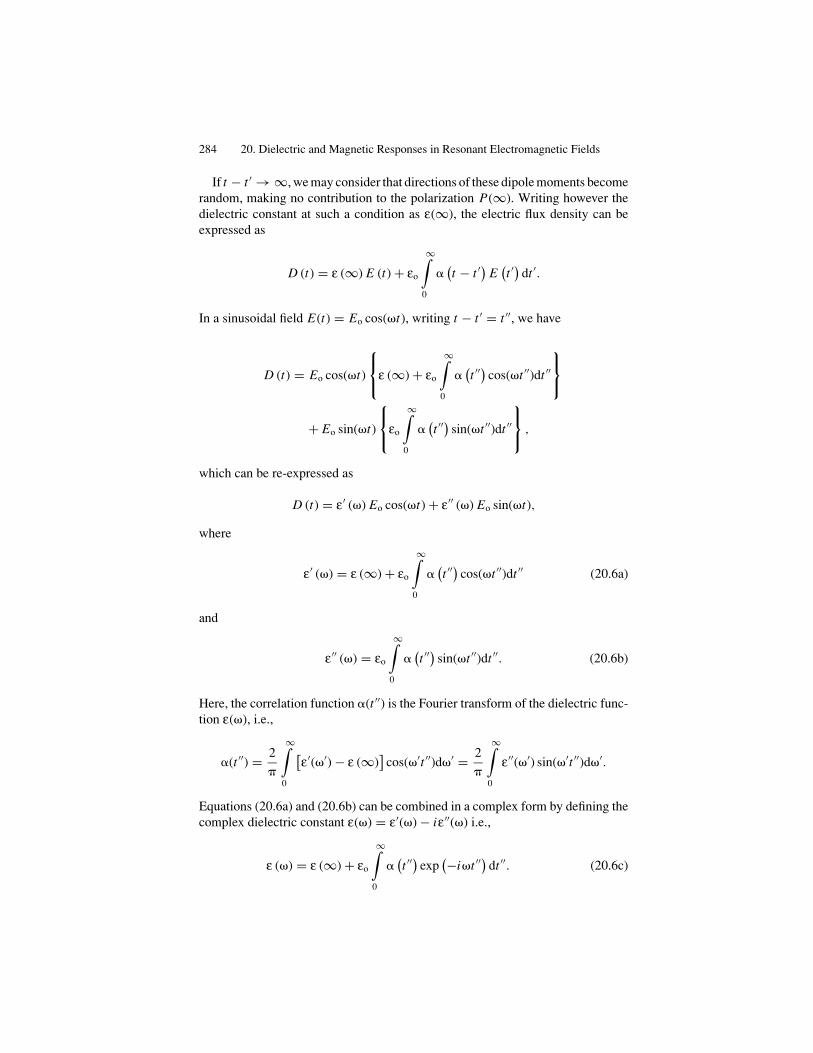
284 20. Dielectric and Magnetic Responses in Resonant Electromagnetic Fields
If t − t ′ → ∞, we may consider that directions of these dipole moments becomerandom, making no contribution to the polarization P(∞). Writing however thedielectric constant at such a condition as ε(∞), the electric flux density can beexpressed as
D (t) = ε (∞) E (t) + εo
∞∫0
�(t − t ′) E
(t ′) dt ′.
In a sinusoidal field E(t) = Eo cos(�t), writing t − t ′ = t ′′, we have
D (t) = Eo cos(�t)
⎧⎨⎩ε (∞) + εo
∞∫0
�(t ′′) cos(�t ′′)dt ′′
⎫⎬⎭
+ Eo sin(�t)
⎧⎨⎩εo
∞∫0
�(t ′′) sin(�t ′′)dt ′′
⎫⎬⎭ ,
which can be re-expressed as
D (t) = ε′ (�) Eo cos(�t) + ε′′ (�) Eo sin(�t),
where
ε′ (�) = ε (∞) + εo
∞∫0
�(t ′′) cos(�t ′′)dt ′′ (20.6a)
and
ε′′ (�) = εo
∞∫0
�(t ′′) sin(�t ′′)dt ′′. (20.6b)
Here, the correlation function �(t ′′) is the Fourier transform of the dielectric func-tion ε(�), i.e.,
�(t ′′) = 2
�
∞∫0
[ε′(�′) − ε (∞)
]cos(�′t ′′)d�′ = 2
�
∞∫0
ε′′(�′) sin(�′t ′′)d�′.
Equations (20.6a) and (20.6b) can be combined in a complex form by defining thecomplex dielectric constant ε(�) = ε′(�) − iε′′(�) i.e.,
ε (�) = ε (∞) + εo
∞∫0
�(t ′′) exp
(−i�t ′′) dt ′′. (20.6c)

Dielectric Relaxation 285
Putting the expressions of �(t ′′) back into (20.5a) and (20.6b), we obtain theKramers–Kronig relations:
ε′ (�) − ε (∞) = 2
�
∞∫0
ε′′ (�′)�′2 − �2
d�′
and
ε′′ (�) = 2
�
∞∫0
ε′ (�′) − ε (∞)
�′2 − �2d�′,
indicating that the respective real and imaginary components ε′ (�) and ε′′ (�) arenot independent.
In a static case signified by � = 0 from (20.6.a) and (20.6.b) we have
ε′ (0) = ε (∞) + εo
∞∫0
�(t ′′)dt ′′ and ε′′ (0) = 0. (20.6d)
Using �(t ′′) = exp(− t ′′
�) in (20.6c) and (20.6d), the integrated results are
ε (�) − ε (∞) = εo�
1 + i��and ε′ (0) − ε (∞) = εo�,
hence we can write the relation for the complex ε(�)gnd ε(0), i.e.,
ε (�) − ε (∞) = ε (0) − ε (∞)
1 + i��. (20.7)
For the real and imaginary parts, we have
ε′ (�) = ε (∞) + ε (0) − ε (∞)
1 + �2� 2
and
ε′′ (�) = [ε (0) − ε (∞)]��
1 + �2� 2,
respectively. Eliminating �� from these expressions for ε′(�) and ε′′(�), we obtainthe formula{
ε′ (�) − ε (0) + ε (∞)
2
}2
+ ε′′ (�)2 ={
ε (0) − ε (∞)
2
}2
, (20.8)
indicating that the curve of ε′(�) vs. ε′′(�), if plotted as a function of fre-
quency �, is a semi-circle of radius r = ε (0) − ε (∞)
2centered at a point
A( 12 {ε (0) + ε (∞)} , 0) on the real ε′-axis, as shown in Figure 20.1. Such a di-
agram, called the Cole-Cole plot, is typical for a dielectric relaxation, which isalso referred to as relaxation of Debye’s type, a useful model for evaluating therelaxation time � .

286 20. Dielectric and Magnetic Responses in Resonant Electromagnetic Fields
FIGURE 20.1. Cole-Cole plot for acomplex dielectric functionε(�) = ε′(�) + ε′′(�).
The dielectric response is not always of Debye’s type, for the kinetic energy ofdipoles can often exceed the frictional energy for relaxation. Typically, the motionis oscillatory around the equilibrium position, as described by the equation ofmotion
md2x
dt2+ �
dx
dt+ kx = eEo exp(i�t)
if in one-dimension, where m, � , k, and e are mass, damping constant, restoringparameter, and charge, respectively. Writing this equation as
d2x
dt2+ �
dx
dt+ �2
ox = eEo
mexp(i�t),
where � /m that would result in the second term is redefined as � , and where�o = √
k/m is the characteristic frequency, the response function can be obtainedfrom the stationary solution as
� (�) ∝ e/m
�2o − �2 + i��
∝ �2o − �2 − i��(
�2o − �2
)2 + �2� 2.
Using this �(�), the flux density can be expressed as
D(�, t) = ε(∞)Eo exp(i�t) + εo�(�)Eo exp(i�t)
={
ε (∞) + �2o − �2
(�2
o − �2)2 + �2� 2
}Eo cos(�t)
− i�� Eo sin(�t)(�2
o − �2)2 + �2� 2
.
Therefore the complex dielectric constant can be given in complex form ε(�) =ε′(�) − iε′′(�), where ε′(�) and ε′′(�) are expressed by
ε′ (�) = ε (∞) + εo�2
o − �2
(�2
o − �2)2 + �2� 2
(20.9a)
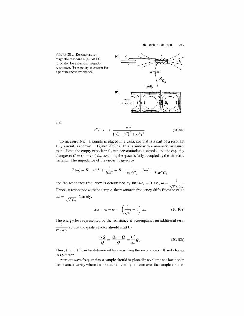
Dielectric Relaxation 287
FIGURE 20.2. Resonators formagnetic resonance. (a) An LCresonator for a nuclear magneticresonance. (b) A cavity resonator fora paramagnetic resonance.
and
ε′′ (�) = εo��(
�2o − �2
)2 + �2� 2. (20.9b)
To measure ε(�), a sample is placed in a capacitor that is a part of a resonantLCo circuit, as shown in Figure 20.2(a). This is similar to a magnetic measure-ment. Here, the empty capacitor Co can accommodate a sample, and the capacitychanges to C = (ε′ − iε′′)Co, assuming the space is fully occupied by the dielectricmaterial. The impedance of the circuit is given by
Z (�) = R + i�L + 1
i�C= R + 1
�ε′′Co+ i�L − 1
i�ε′′Co,
and the resonance frequency is determined by ImZ (�) = 0, i.e., � = 1√ε′LCo
.
Hence, at resonance with the sample, the resonance frequency shifts from the value
�o = 1√LCo
. Namely,
�� = � − �o =(
1√ε′ − 1
)�o. (20.10a)
The energy loss represented by the resistance R accompanies an additional term1
ε′′ �Coso that the quality factor should shift by
�Q
Q= Qo − Q
Q= ε′′
εoQo. (20.10b)
Thus, ε′ and ε′′ can be determined by measuring the resonance shift and changein Q-factor.
At microwave frequencies, a sample should be placed in a volume at a location inthe resonant cavity where the field is sufficiently uniform over the sample volume.

288 20. Dielectric and Magnetic Responses in Resonant Electromagnetic Fields
In this case, the volume ratio, i.e., sample/cavity, must be calibrated for the formula(20.10a) and (20.10b) to provide reliable values of ε′ and ε′′.
20.4. Magnetic Resonance
Figure 20.2 illustrates resonators for magnetic studies, similar to what are usedfor dielectric measurements. In such a resonator, a sample is placed at a locationwhere the magnetic flux density is high: inside a coil at low frequencies, as shownin Figure 20.2(a), and at the location indicated in Figure 20.2(b) for microwavemeasurements. At these locations the flux density is also assumed to be sufficientlyuniform over the sample volume.
Magnetic moments originate from unpaired electrons of ions in specific groupsof elements. The electronic motion in ions is much faster than the dipole moments,as signified by a distinctive difference in their relaxation times. It is also knownthat various atomic nuclei are characterized by their magnetic moments. Virtuallyindependent of the host material, the properties of these ions and nuclei can beinvestigated under an adiabatic condition with applied magnetic fields.
Hence, a magnetic moment in non-magnetic media can be regarded as primarilyisolated from the rest of the material and can be set in precession when a staticmagnetic field is applied. In the presence of a uniform magnetic field Bo, thereis a torque × Bo exerted on such a magnetic moment as described by theequation of motion
dJ
dt= × Bo,
where J is the angular momentum of a carrier of . Writing = � J, where � iscalled the gyromagnetic ratio, we have
d
dt= � ( × Bo) . (20.11a)
Using rectangular coordinates x, y, z with respect to the direction of Bo, which istaken as the z-axis as shown in Figure 20.3, equation (20.11) can be expressed as
dx
dt= �y Bo,
dy
dt= −�x Bo and
dz
dt= 0. (20.11b)
From the last equation, z can be a constant of motion, i.e.,
z = const, (20.12a)
whereas for perpendicular components x and y , combining the first and secondequations in (20.11b) in complex form gives
d(x + iy
)dt
= � Bo(y − ix
) = −i� Bo(x + iy
),
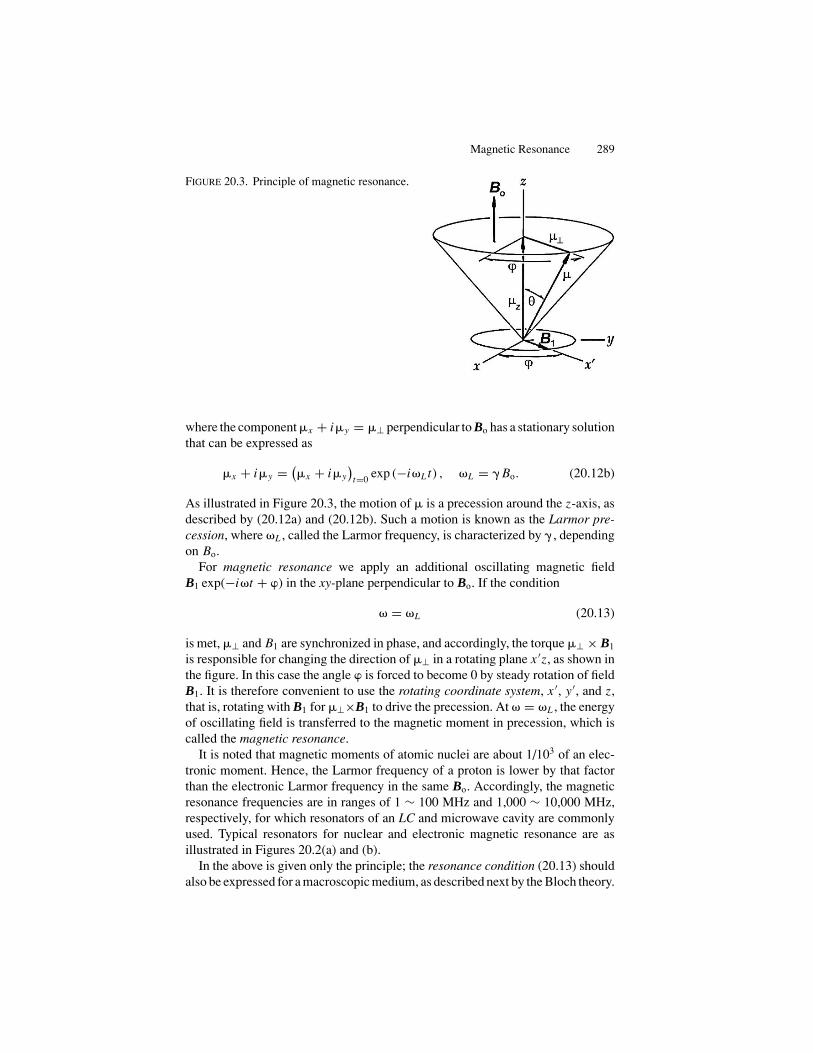
Magnetic Resonance 289
FIGURE 20.3. Principle of magnetic resonance.
where the component x + iy = ⊥ perpendicular to Bo has a stationary solutionthat can be expressed as
x + iy = (x + iy
)t=0 exp (−i�L t) , �L = � Bo. (20.12b)
As illustrated in Figure 20.3, the motion of is a precession around the z-axis, asdescribed by (20.12a) and (20.12b). Such a motion is known as the Larmor pre-cession, where �L , called the Larmor frequency, is characterized by � , dependingon Bo.
For magnetic resonance we apply an additional oscillating magnetic fieldB1 exp(−i�t + ) in the xy-plane perpendicular to Bo. If the condition
� = �L (20.13)
is met, ⊥ and B1 are synchronized in phase, and accordingly, the torque ⊥ × B1
is responsible for changing the direction of ⊥ in a rotating plane x ′z, as shown inthe figure. In this case the angle is forced to become 0 by steady rotation of fieldB1. It is therefore convenient to use the rotating coordinate system, x ′, y′, and z,that is, rotating with B1 for ⊥×B1 to drive the precession. At � = �L , the energyof oscillating field is transferred to the magnetic moment in precession, which iscalled the magnetic resonance.
It is noted that magnetic moments of atomic nuclei are about 1/103 of an elec-tronic moment. Hence, the Larmor frequency of a proton is lower by that factorthan the electronic Larmor frequency in the same Bo. Accordingly, the magneticresonance frequencies are in ranges of 1 ∼ 100 MHz and 1,000 ∼ 10,000 MHz,respectively, for which resonators of an LC and microwave cavity are commonlyused. Typical resonators for nuclear and electronic magnetic resonance are asillustrated in Figures 20.2(a) and (b).
In the above is given only the principle; the resonance condition (20.13) shouldalso be expressed for a macroscopic medium, as described next by the Bloch theory.
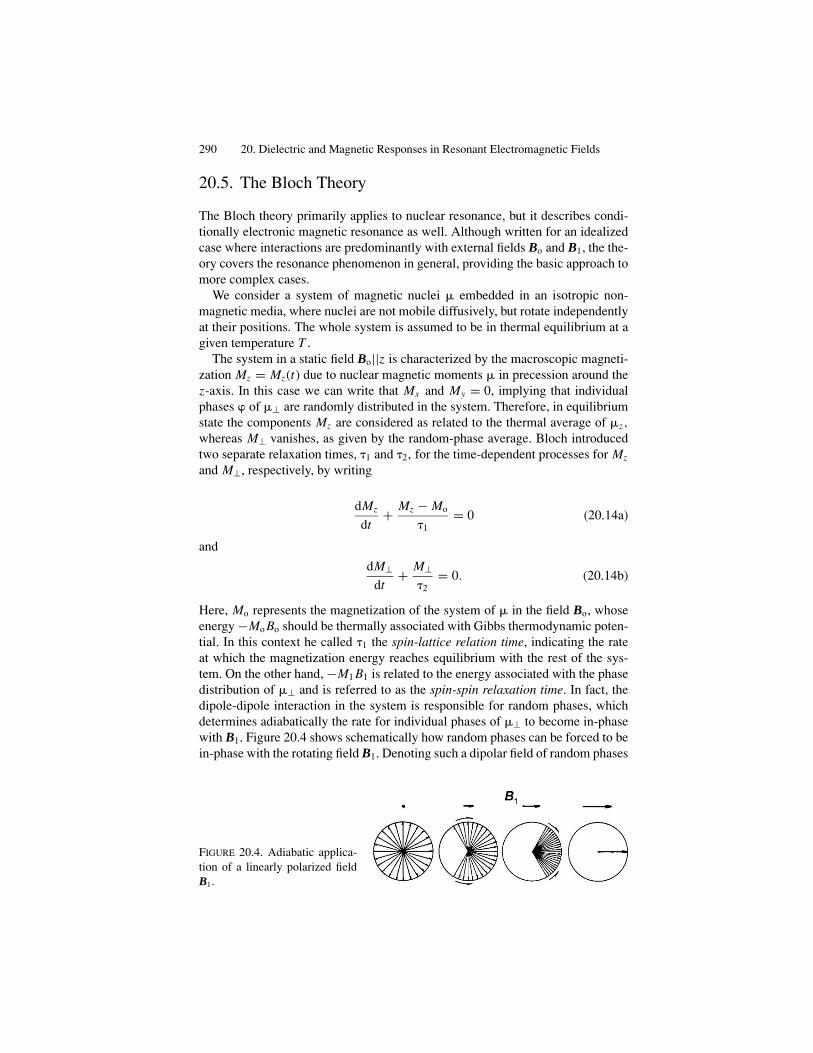
290 20. Dielectric and Magnetic Responses in Resonant Electromagnetic Fields
20.5. The Bloch Theory
The Bloch theory primarily applies to nuclear resonance, but it describes condi-tionally electronic magnetic resonance as well. Although written for an idealizedcase where interactions are predominantly with external fields Bo and B1, the the-ory covers the resonance phenomenon in general, providing the basic approach tomore complex cases.
We consider a system of magnetic nuclei embedded in an isotropic non-magnetic media, where nuclei are not mobile diffusively, but rotate independentlyat their positions. The whole system is assumed to be in thermal equilibrium at agiven temperature T .
The system in a static field Bo||z is characterized by the macroscopic magneti-zation Mz = Mz(t) due to nuclear magnetic moments in precession around thez-axis. In this case we can write that Mx and My = 0, implying that individualphases of ⊥ are randomly distributed in the system. Therefore, in equilibriumstate the components Mz are considered as related to the thermal average of z,
whereas M⊥ vanishes, as given by the random-phase average. Bloch introducedtwo separate relaxation times, �1 and �2, for the time-dependent processes for Mz
and M⊥, respectively, by writing
dMz
dt+ Mz − Mo
�1= 0 (20.14a)
and
dM⊥dt
+ M⊥�2
= 0. (20.14b)
Here, Mo represents the magnetization of the system of in the field Bo, whoseenergy −Mo Bo should be thermally associated with Gibbs thermodynamic poten-tial. In this context he called �1 the spin-lattice relation time, indicating the rateat which the magnetization energy reaches equilibrium with the rest of the sys-tem. On the other hand, −M1 B1 is related to the energy associated with the phasedistribution of ⊥ and is referred to as the spin-spin relaxation time. In fact, thedipole-dipole interaction in the system is responsible for random phases, whichdetermines adiabatically the rate for individual phases of ⊥ to become in-phasewith B1. Figure 20.4 shows schematically how random phases can be forced to bein-phase with the rotating field B1. Denoting such a dipolar field of random phases
FIGURE 20.4. Adiabatic applica-tion of a linearly polarized fieldB1.

The Bloch Theory 291
by �B, it is clear that the applied B1 should be greater than �B in order to unify dis-tributed phases. Writing �B ∼ 1/��2, the condition B1 � �B can be expressedas
� B1 � 1/�2, (20.15)
which is called the slow passage condition, signifying that an external field B1 isapplied adiabatically. In fact, (20.14b) is a valid assumption under the slow passagecondition. Such an adiabatic phasing as shown in Figure 20.4 is reversible, andhence dephasing should take place when external B1 is switched off.
Taking these relaxation mechanisms into account, Bloch wrote the equations ofmotion in the presence of Bo and B1exp(±i�t) as
dM±dt
± i� Bo M± + M±�2
= −i Mz Bo exp (±i�t) (20.16a)
and
dMz
dt+ Mz − Mo
�1= 1
2i� B1
[M+ exp (−i�t) + M− exp(i�t)
]. (20.16b)
It is noted that (20.16a) and (20.16b), known as the Bloch equations, havestationary solutions under a slow passage condition if one assumes that dMz
dt = 0and M⊥ = M± ∝ exp(±i�t). With respect to the rotating coordinate system, Mz
and M± can be related as
M± (t) = � B1 Mz exp (±i�t)
� + �L ∓ i�2
, where �L = � Bo.
Accordingly,
Mz
Mo= 1 + (� − �L )2 � 2
2
1 + (� − �L )2 � 22 + � 2 B2
1 �1�2(20.17a)
and
M±Mo
= [(� − �L ) �2 ± i] � B1�2 exp (±i�t)
1 + (� − �L )2 � 22 + � 2 B2
1 �1�2. (20.17b)
Equation (20.17a) indicates that Mz ≈ Mo at resonance, i.e., � = �L , providedthat � B2
1 �1�2 � 1. In this case we have
tan � = M±Mz
≈ � B1�2
1 + (� − �L )2 � 22
.
The complex magnetic response function � (�) can be defined from the relation
M± = � (�) B1 exp (±i�t) and Mo = �o Bo,
and we have
�± (�)
�o= � Bo�2 {(� − �L ) �2 + i}
1 + (� − �L )2 � 22 + � 2 B2
1 �1�2.
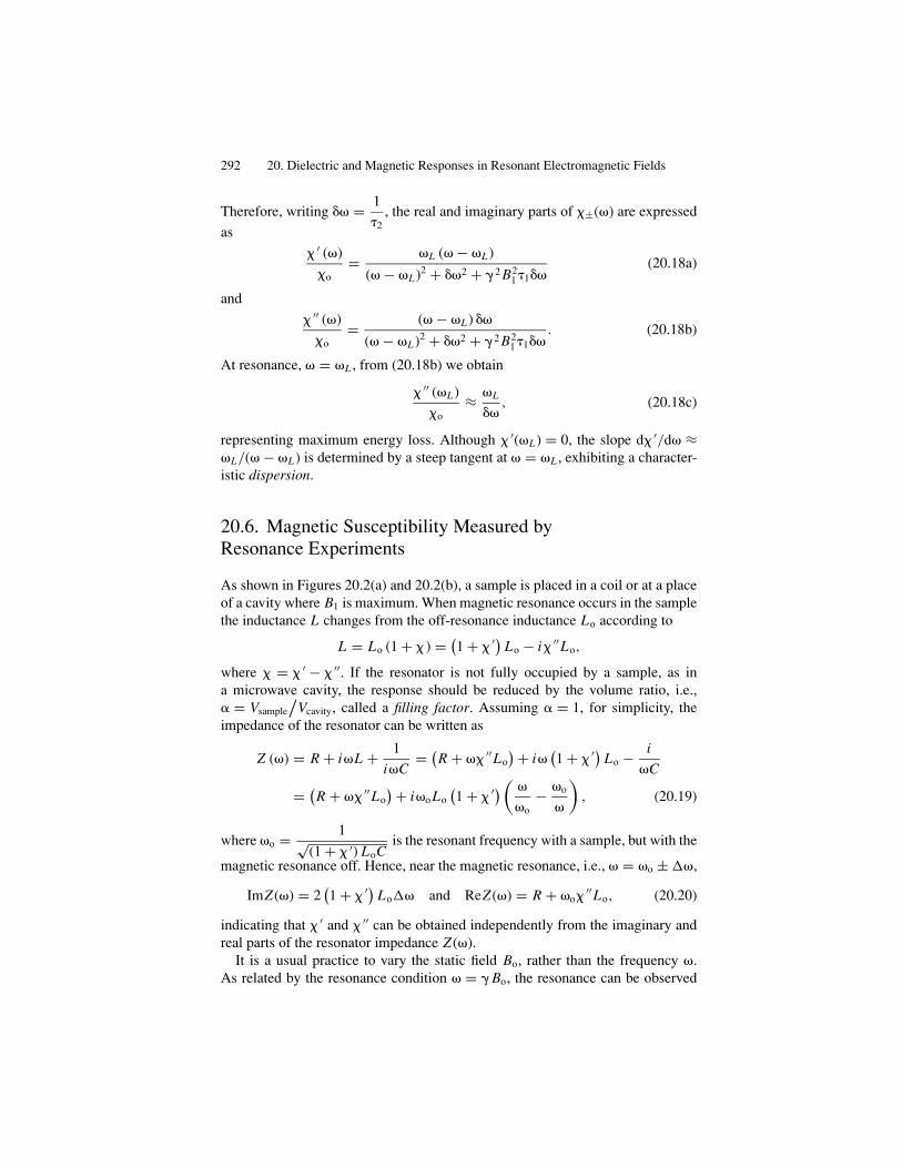
292 20. Dielectric and Magnetic Responses in Resonant Electromagnetic Fields
Therefore, writing �� = 1
�2, the real and imaginary parts of �±(�) are expressed
as
� ′ (�)
�o= �L (� − �L )
(� − �L )2 + ��2 + � 2 B21 �1��
(20.18a)
and
� ′′ (�)
�o= (� − �L ) ��
(� − �L )2 + ��2 + � 2 B21 �1��
. (20.18b)
At resonance, � = �L , from (20.18b) we obtain
� ′′ (�L )
�o≈ �L
��, (20.18c)
representing maximum energy loss. Although � ′(�L ) = 0, the slope d� ′/d� ≈�L/(� − �L ) is determined by a steep tangent at � = �L , exhibiting a character-istic dispersion.
20.6. Magnetic Susceptibility Measured byResonance Experiments
As shown in Figures 20.2(a) and 20.2(b), a sample is placed in a coil or at a placeof a cavity where B1 is maximum. When magnetic resonance occurs in the samplethe inductance L changes from the off-resonance inductance Lo according to
L = Lo (1 + � ) = (1 + � ′) Lo − i� ′′Lo,
where � = � ′ − � ′′. If the resonator is not fully occupied by a sample, as ina microwave cavity, the response should be reduced by the volume ratio, i.e.,� = Vsample
/Vcavity, called a filling factor. Assuming � = 1, for simplicity, the
impedance of the resonator can be written as
Z (�) = R + i�L + 1
i�C= (
R + �� ′′Lo) + i�
(1 + � ′) Lo − i
�C
= (R + �� ′′Lo
) + i�oLo(1 + � ′) (
�
�o− �o
�
), (20.19)
where �o = 1√(1 + � ′) LoC
is the resonant frequency with a sample, but with the
magnetic resonance off. Hence, near the magnetic resonance, i.e., � = �o ± ��,
ImZ (�) = 2(1 + � ′) Lo�� and ReZ (�) = R + �o� ′′Lo, (20.20)
indicating that � ′ and � ′′ can be obtained independently from the imaginary andreal parts of the resonator impedance Z (�).
It is a usual practice to vary the static field Bo, rather than the frequency �.As related by the resonance condition � = � Bo, the resonance can be observed
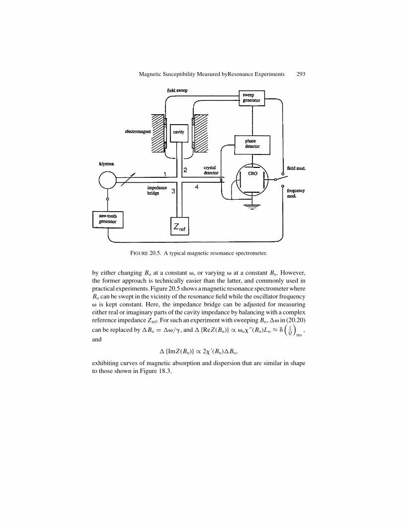
Magnetic Susceptibility Measured byResonance Experiments 293
FIGURE 20.5. A typical magnetic resonance spectrometer.
by either changing Bo at a constant �, or varying � at a constant Bo. However,the former approach is technically easier than the latter, and commonly used inpractical experiments. Figure 20.5 shows a magnetic resonance spectrometer whereBo can be swept in the vicinity of the resonance field while the oscillator frequency� is kept constant. Here, the impedance bridge can be adjusted for measuringeither real or imaginary parts of the cavity impedance by balancing with a complexreference impedance Zref. For such an experiment with sweeping Bo, �� in (20.20)
can be replaced by �Bo = ��/� , and � {ReZ (Bo)} ∝ �o� ′′(Bo)Lo ≈ �(
1Q
)res
,
and
� {ImZ (Bo)} ∝ 2� ′(Bo)�Bo,
exhibiting curves of magnetic absorption and dispersion that are similar in shapeto those shown in Figure 18.3.

21Laser Oscillations, Phase Coherence,and Photons
21.1. Optical Resonators
Phase-coherent radiation at high frequencies is a useful signal carrier for telecom-munication and guidance. While wave propagation at high frequencies dependson many factors; frequency range is usually selected for specific purposes. For ex-ample, u.h.f. waves (108 ∼ 109 Hz) and microwaves (109 ∼ 1011 Hz) at moderatepower levels are indispensable for practical applications because of the high mod-ulating capabilities and directivity; yet, energy dissipation in air space is a seriousproblem at all frequencies. Optical waves could also be used in telecommunica-tions, in principle, but their use for such purposes was not imaginable before 1958,when Schawlow, Townes, and Prokorov demonstrated that radiation from excitedatoms and molecules could be incorporated with optical resonators. Originatingfrom quantum transitions, optical radiation is normally incoherent, hence, it isnot suitable for any purpose requiring coherent radiation. However, the successfulexperiments by Schawlow et al. on simultaneous emission from excited atoms andmolecules opened an entirely new era of telecommunication.
As it relates to quantum transitions, coherent optical radiation is a subject beyondthe scope of classical physics; but the concept is simple enough to accept by today’sstandards, unless deeper insight is sought in understanding its origin. Therefore,we can be free to discuss quantum transitions for optical waves—even using asemi-classical approach to this recent application.
The Maxwell theory is well established for classical electromagnetism; however,as applied to higher frequency phenomena in the infrared and visible wave ranges,we encounter a limitation that arises from radiation sources that is predominantlyquantum in nature. It is important to realize that classical theory has a limitationdue to microscopic interactions. Thus “laser” oscillators pose a technical problemfor incoherency, related to uncertainity in observing the phase of radiation, a signof quantum character of electromagnetic phenomena.
In this chapter we conclude our treatment of classical electromagnetism with abrief discussion of optical oscillators. Like a microwave cavity, an optical resonatorcould be fabricated to accommodate many wavelengths, in principle. For example,in an optical cavity of size 1 cm3 there should be as many as 108 normal modes
294
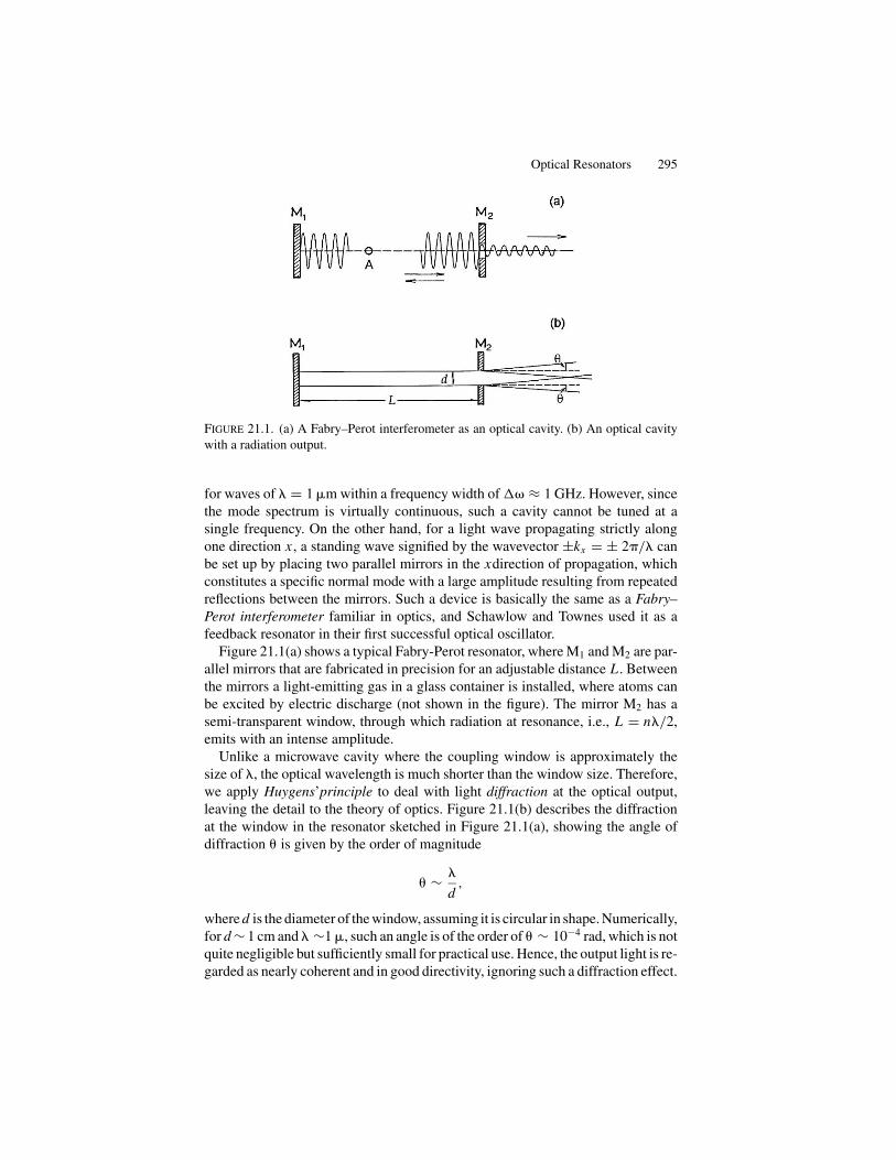
Optical Resonators 295
FIGURE 21.1. (a) A Fabry–Perot interferometer as an optical cavity. (b) An optical cavity
with a radiation output.
for waves of � = 1 �m within a frequency width of �� ≈ 1 GHz. However, sincethe mode spectrum is virtually continuous, such a cavity cannot be tuned at asingle frequency. On the other hand, for a light wave propagating strictly alongone direction x , a standing wave signified by the wavevector ±kx = ± 2�/� canbe set up by placing two parallel mirrors in the xdirection of propagation, whichconstitutes a specific normal mode with a large amplitude resulting from repeatedreflections between the mirrors. Such a device is basically the same as a Fabry–Perot interferometer familiar in optics, and Schawlow and Townes used it as afeedback resonator in their first successful optical oscillator.
Figure 21.1(a) shows a typical Fabry-Perot resonator, where M1 and M2 are par-allel mirrors that are fabricated in precision for an adjustable distance L . Betweenthe mirrors a light-emitting gas in a glass container is installed, where atoms canbe excited by electric discharge (not shown in the figure). The mirror M2 has asemi-transparent window, through which radiation at resonance, i.e., L = n�/2,emits with an intense amplitude.
Unlike a microwave cavity where the coupling window is approximately thesize of �, the optical wavelength is much shorter than the window size. Therefore,we apply Huygens’principle to deal with light diffraction at the optical output,leaving the detail to the theory of optics. Figure 21.1(b) describes the diffractionat the window in the resonator sketched in Figure 21.1(a), showing the angle ofdiffraction � is given by the order of magnitude
� ∼ �
d,
where d is the diameter of the window, assuming it is circular in shape. Numerically,for d ∼ 1 cm and � ∼1 �, such an angle is of the order of � ∼ 10−4 rad, which is notquite negligible but sufficiently small for practical use. Hence, the output light is re-garded as nearly coherent and in good directivity, ignoring such a diffraction effect.

296 21. Laser Oscillations, Phase Coherence, and Photons
21.2. Quantum Transitions
Light emitting atoms and molecules must be treated quantum mechanically, al-though some related phenomena can be discussed within the classical theory. Themost serious difficulty in the classical theory is that the electron orbit cannotremain stable, as energy is continuously lost by emitting radiation. In quantumtheory, on the other hand, stability is assured by discrete energy levels of station-ary orbits, while transitions between levels are restricted by so-called “selectionrules.” Therefore, such microscopic systems can release their radiation energy ifthey are in excited levels above the ground state; such natural radiation of a finitelife is referred to as spontaneous radiation. On the other hand, those in the groundstate can in no way lose energy, so remain stable.
If permitted by the selection rule, a transition occurs spontaneously betweenatomic levels Ej and Ei, where Ej > Ei, emitting radiation at a frequency �ji
determined by
�ji = 1
h
(Ej − Ei
), (21.1)
where h = h/
2� = 1.0 × 10⁻³⁴ J-sec is the Planck constant h divided by 2�.Spontaneous radiation can be interpreted classically as related to an oscillatingelectric dipole moment
p(t) = Io
i�ji
exp(i�jit), where po = Io
i�ji
,
representing an effective circular current in a loop antenna, as discussed in Section13.3. We can calculate such radiation energy emitted during one complete circularmotion as
�E = cpo2k4
12�εo
2�
�ji
= po2�ji
3
6εoc3∝
(�ji
c
)3
, (21.2)
which is called the spontaneous emission, and � = h
�Eis the lifetime of the
excited state Ej. Hence, the transition is not sharply observed, but broadened to�� ∼ h/� . It is noted that the probability for the transition (21.2) is proportionalto (�ji/c)3, which is significant if �ji are optical frequencies or higher, whereasat radio- and microwave frequencies, such spontaneous emission probability isnegligibly small.
In practice, those excited atoms cannot be quite independent in gaseous states,but interact with each other, so that spontaneous transitions do not occur normally ata sharp frequency, but are broadened at �ji. In addition to the natural broadening�� ∼ h/� due to lifetime of the excite state, a line broadening arises not onlyfrom collisions with other atoms, known as the pressure broadening, but also fromrelative motion with respect to a point of observation, called Doppler broadening.Typically, the overall lifetime of light-emitting atoms is of the order of 10−9 s or
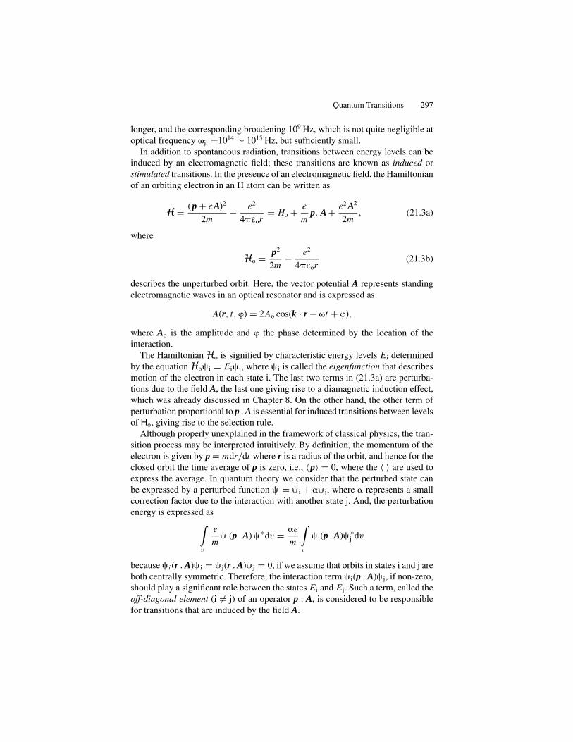
Quantum Transitions 297
longer, and the corresponding broadening 109 Hz, which is not quite negligible atoptical frequency �ji =1014 ∼ 1015 Hz, but sufficiently small.
In addition to spontaneous radiation, transitions between energy levels can beinduced by an electromagnetic field; these transitions are known as induced orstimulated transitions. In the presence of an electromagnetic field, the Hamiltonianof an orbiting electron in an H atom can be written as
H = (p + eA)2
2m− e2
4�εor= Ho + e
mp. A + e2 A2
2m, (21.3a)
where
Ho = p2
2m− e2
4�εor(21.3b)
describes the unperturbed orbit. Here, the vector potential A represents standingelectromagnetic waves in an optical resonator and is expressed as
A(r, t, �) = 2Ao cos(k · r − �t + �),
where Ao is the amplitude and � the phase determined by the location of theinteraction.
The Hamiltonian Ho is signified by characteristic energy levels Ei determinedby the equation Ho i = Ei i, where i is called the eigenfunction that describesmotion of the electron in each state i. The last two terms in (21.3a) are perturba-tions due to the field A, the last one giving rise to a diamagnetic induction effect,which was already discussed in Chapter 8. On the other hand, the other term ofperturbation proportional to p . A is essential for induced transitions between levelsof Ho, giving rise to the selection rule.
Although properly unexplained in the framework of classical physics, the tran-sition process may be interpreted intuitively. By definition, the momentum of theelectron is given by p = mdr/dt where r is a radius of the orbit, and hence for theclosed orbit the time average of p is zero, i.e., 〈p〉 = 0, where the 〈 〉 are used toexpress the average. In quantum theory we consider that the perturbed state canbe expressed by a perturbed function = i + j, where represents a smallcorrection factor due to the interaction with another state j. And, the perturbationenergy is expressed as∫
v
e
m (p . A) ∗dv = e
m
∫v
i(p . A) ∗j dv
because i (r . A) i = j(r . A) j = 0, if we assume that orbits in states i and j areboth centrally symmetric. Therefore, the interaction term i(p . A) j, if non-zero,should play a significant role between the states Ei and Ej. Such a term, called theoff-diagonal element (i �= j) of an operator p . A, is considered to be responsiblefor transitions that are induced by the field A.
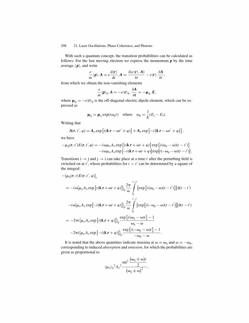
298 21. Laser Oscillations, Phase Coherence, and Photons
With such a quantum concept, the transition probabilities can be calculated asfollows: For the fast moving electron we express the momentum p by the timeaverage 〈 p〉, and write
e
m〈p〉. A = e
d〈r〉dt
. A = ∂(e〈r〉. A)
∂t− e〈r〉. ∂A
∂t,
from which we obtain the non-vanishing elements
e
m〈p〉ij. A = −e〈r〉ij.
∂A∂t
= −�ij. E,
where �ij = −e〈r〉ij is the off-diagonal electric dipole element, which can be ex-pressed as
�ij = �o exp(i�ijt) where �ij = 1
h(Ej − Ei).
Writing that
A(r, t ′, �) = Ao exp[i(k.r − �t ′ + �)
] + Ao exp[−i
(k.r − �t ′ + �
)],
we have
−�ij(r, t ′)E(r, t ′,�) = −i��o Ao exp[i(k.r + �t + �)
]exp
[i(�ij − �)(t − t ′)
]−i��o Ao exp
[−i(k.r + �t + �)]exp
[i(−�ij − �)(t − t ′)
].
Transitions i → j and j → i can take place at a time t after the perturbing field isswitched on at t ′, whose probabilities for t > t ′ can be determined by a square ofthe integral:
−⟨�ij(r, t)E(r, t ′, �)
⟩t
= −i�⟨�o Ao exp
[i(k.r + �t + �)
]⟩ij
2�
�
t−t ′∫0
{exp
[i(�ij − �)(t − t ′)
]}d(t − t ′)
−i�⟨�o Ao exp
[−i(k.r + �t + �)]⟩
ji
2�
�
t−t ′∫0
{exp
[i(−�ji − �)(t − t ′)
]}d(t − t ′)
= −2�i⟨�o Ao exp
[i(k.r + �)
]⟩ij
exp[i(�ij − �)t
] − 1
�ij − �
−2�i⟨�o Ao exp
[−i(k.r + �)]⟩
ji
exp[i(−�ji − �)t
] − 1
−�ji − �.
It is noted that the above quantities indicate maxima at � = �ij and � = −�ji,corresponding to induced absorption and emission, for which the probabilities aregiven as proportional to
〈�o〉ij2 Ao
2sin2
(�ij ∓ �
)t
2(�ij ∓ �
)2,

Inverted Population and the Negative Temperature 299
which are equal for both absorption and emission at � = ∓�ij, and proportional toAo
2 and 〈�o〉ij2. In such an interpretation the electromagnetic field can be assumed
as consisting of energy quanta h�ij that are absorbed or emitted between atomicenergy levels, as Ei
→← Ej, obeying the energy conservation law.
21.3. Inverted Population and the Negative Temperature
Einstein (1917) proposed the relation between probabilities for induced transitionsand spontaneous emission, giving the thermodynamic foundation to Planck’s the-ory of blackbody radiation. His formula can deal with the light emission andabsorption in a body in thermal equilibrium with its surroundings.
Considering a system of two energies Ei and Ej in a body in equilibrium attemperature T , these levels are occupied by Ni and Nj atoms determined by theBoltzmann statistics, i.e.,
Ni
Nj
= exp
(− Ei − Ej
kBT
), (21.4)
where kB = 1.38066 × 10⁻²³J-K−1 is the Boltzmann constant, signifying that al-ways Ni < Nj in equilibrium if Ei > Ej. However, if the atoms can absorb lightquanta h�ij at a rate sufficiently faster than the relaxation rate, a condition forNi > Nj can be achieved at which the temperature takes a negative value accord-ing to (21.4), i.e., T < 0.
When absorbing radiation quanta, the population Ni at the upper level increases,while the population Nj at the lower level decreases. For such a pumping processthat may be in equilibrium with the radiation field, Einstein gave the formula forthe radiation power,
P(�ij) = h�ij
[Ni Aij + (Ni − Nj)Bij � (�ij)
], (21.5)
where Aij and Bij are called the Einstein coefficients for spontaneous and inducedemissions, respectively, and � (�ij) the radiation energy density. Denoting the ex-cited and ground states by i and j as in the above, we have Ni Nj at a normaltemperature, so that the second negative term dominates the power P(�ij) in (21.5).Therefore, such a system can absorb radiation quanta under normal circumstances,where the first term for emission is significant if the value of � (�ij) is small. On theother hand, when � (�ij) is large the second term for induced transitions becomessignificant. At radio- and microwave frequencies, the spontaneous transition isnegligible, and only induced transitions are predominant for the pumping process.However, at optical frequencies the factor � (�ij) is not negligible, and hence thepumping rate Aij should be sufficiently high to achieve a condition for Ni > Nj.
In any case, the condition for inverted population is necessary for simultaneousemissions from the excited states, from which coherent radiation can be stimu-lated by an oscillating electric field of a resonator that is incorporated with anatomic system. Referring to the Boltzmann formula (21.4), such a state of invertedpopulations can be characterized by a negative temperature −T . Nevertheless,
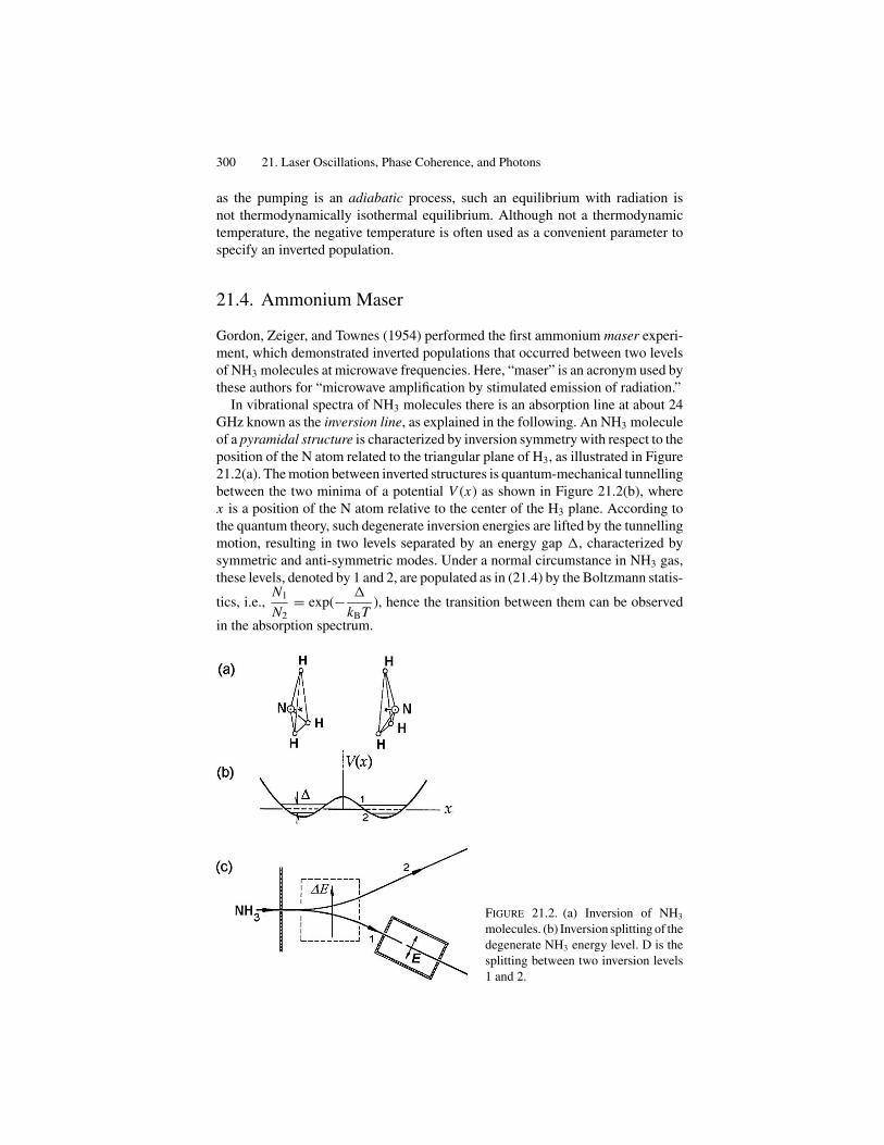
300 21. Laser Oscillations, Phase Coherence, and Photons
as the pumping is an adiabatic process, such an equilibrium with radiation isnot thermodynamically isothermal equilibrium. Although not a thermodynamictemperature, the negative temperature is often used as a convenient parameter tospecify an inverted population.
21.4. Ammonium Maser
Gordon, Zeiger, and Townes (1954) performed the first ammonium maser experi-ment, which demonstrated inverted populations that occurred between two levelsof NH3 molecules at microwave frequencies. Here, “maser” is an acronym used bythese authors for “microwave amplification by stimulated emission of radiation.”
In vibrational spectra of NH3 molecules there is an absorption line at about 24GHz known as the inversion line, as explained in the following. An NH3 moleculeof a pyramidal structure is characterized by inversion symmetry with respect to theposition of the N atom related to the triangular plane of H3, as illustrated in Figure21.2(a). The motion between inverted structures is quantum-mechanical tunnellingbetween the two minima of a potential V (x) as shown in Figure 21.2(b), wherex is a position of the N atom relative to the center of the H3 plane. According tothe quantum theory, such degenerate inversion energies are lifted by the tunnellingmotion, resulting in two levels separated by an energy gap �, characterized bysymmetric and anti-symmetric modes. Under a normal circumstance in NH3 gas,these levels, denoted by 1 and 2, are populated as in (21.4) by the Boltzmann statis-
tics, i.e.,N1
N2
= exp(− �
kBT), hence the transition between them can be observed
in the absorption spectrum.
FIGURE 21.2. (a) Inversion of NH3
molecules. (b) Inversion splitting of the
degenerate NH3 energy level. D is the
splitting between two inversion levels
1 and 2.
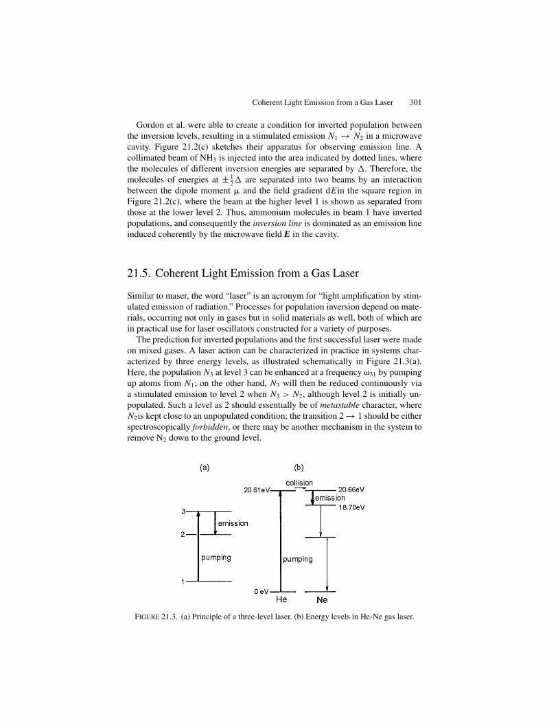
Coherent Light Emission from a Gas Laser 301
Gordon et al. were able to create a condition for inverted population betweenthe inversion levels, resulting in a stimulated emission N1 → N2 in a microwavecavity. Figure 21.2(c) sketches their apparatus for observing emission line. Acollimated beam of NH3 is injected into the area indicated by dotted lines, wherethe molecules of different inversion energies are separated by �. Therefore, themolecules of energies at ± 1
2� are separated into two beams by an interaction
between the dipole moment � and the field gradient dE in the square region inFigure 21.2(c), where the beam at the higher level 1 is shown as separated fromthose at the lower level 2. Thus, ammonium molecules in beam 1 have invertedpopulations, and consequently the inversion line is dominated as an emission lineinduced coherently by the microwave field E in the cavity.
21.5. Coherent Light Emission from a Gas Laser
Similar to maser, the word “laser” is an acronym for “light amplification by stim-ulated emission of radiation.” Processes for population inversion depend on mate-rials, occurring not only in gases but in solid materials as well, both of which arein practical use for laser oscillators constructed for a variety of purposes.
The prediction for inverted populations and the first successful laser were madeon mixed gases. A laser action can be characterized in practice in systems char-acterized by three energy levels, as illustrated schematically in Figure 21.3(a).Here, the population N3 at level 3 can be enhanced at a frequency �31 by pumpingup atoms from N1; on the other hand, N3 will then be reduced continuously viaa stimulated emission to level 2 when N3 > N2, although level 2 is initially un-populated. Such a level as 2 should essentially be of metastable character, whereN2is kept close to an unpopulated condition; the transition 2 → 1 should be eitherspectroscopically forbidden, or there may be another mechanism in the system toremove N2 down to the ground level.
FIGURE 21.3. (a) Principle of a three-level laser. (b) Energy levels in He-Ne gas laser.
302 21. Laser Oscillations, Phase Coherence, and Photons
Figure 21.3(b) shows the energy level diagram for a He-Ne gas laser, consistingof these atoms in 90:10 percentage ratio. By applying a high frequency discharge,He atoms are pumped up primarily to the excited level at 20.61 eV above theground state. Excited He atoms collide then with Ne atoms, resulting in excited Ne(2p55s1) at a metastable state. These excited Ne atoms emit red light by inducedtransitions, falling down to a lower level at 18.70 eV, as shown in the diagram.As induced transitions are practically simultaneous, such a red emission light isnearly coherent at the wavelength � = 623.8 nm. Stepwise spontaneous transitionsfrom the level at 18.70 eV can maintain the inverted population ratio between the20.66 eV and 18.70 eV levels for Ne atoms.
By simultaneous pumping by high frequency discharge the subsequent inducedemission can be made practically coherent, although diffraction effects are in-evitable at the output of the instrument in use.
21.6. Phase Coherence and Radiation Quanta
Dynamical properties of plane waves were demonstrated by radiation pressureexperiments. As they exert a force on a charged particle, electromagnetic wavescan be equivalent to n particles of zero mass and momentum p. Here p is linearlyrelated to the kinetic energy K , i.e., K = cp, according to the special theoryof relativity. Quantum theoretically, electromagnetic waves confined to a finitevolume consist of n radiation quanta h�, hence their energy per volume is givenby K = nh�, where n is the density of quanta. On the other hand, according tothe Maxwell theory each wave is characterized by a phase of propagation.
For electromagnetic waves originating from an oscillating charge-current, wegenerally consider that the wavelength is long compared with the size of the source,so no significant diffracted waves are considered for the radiation. In contrast, forwaves at optical or higher frequencies, radiation is characteristically incoherent,as it originates from randomly distributed emitters. Optical radiation from a laseroscillator is practically coherent with a well-tuned resonator; however at the presentlevel of technology it is not an easy task to construct lasers at ultraviolet and evenshorter wavelengths since phase incoherency becomes a more serious problem.
Nevertheless, noting that the classical Maxwell theory has limitations at higherfrequencies, we should realize that in radiation from microscopic sources, phasesare essentially at random, and hence the Poynting vector should be expressed as
P = cu〈U 〉, where U = εo
(∑i
Ei
)·(∑
j
Ej
)∗. (21.6)
Here
Ei = Eoi exp(i�i),
where �i = k · r i − �ti + � is the phase of radiation, in which the shift � signifiesthe phase of emission from a microscopic source in random distribution. Here,
Phase Coherence and Radiation Quanta 303
in reality, P and 〈U 〉 should be subjected not only to the timescale of observationbut also to distributed light sources. At any rate, the energy U in (21.6) can bewritten as
U = εo
∑i
Eoi · Eoi∗ + εo
∑i�=j
Eoi · Eoj∗ exp(i��ij), (21.7)
where ��ij = �i − �j are phase differences between waves from different emitters,signifying incoherence of radiation. The first term on the right of (21.7) representsquantum energy 〈Uo〉 = noh� for ��ij = 0, where no is the number of coherentphotons, and the second term is the energy deviation 〈U 〉 − 〈Uo〉 due to ��ij �= 0,indicating incoherence. Hence, we can write
〈U 〉 − 〈Uo〉 = (n − no)h� = εo
∑i�=j
Eoi2⟨exp(i��ij)
⟩. (21.8)
Assuming that such ��ij are continuously distributed in a range between −��and +��, the average 〈exp(i��ij)〉 in (21.8) can be calculated as
⟨exp(i��ij)
⟩ = 1
2��
+��∫−��
exp(i��)d(��) = cos ��
��≈ 1
��
for a small ��. Therefore, we have
εo〈Ei · Ej〉i�=j = nh�
��. (21.9)
Writing n − no = �n to indicate uncertainty of the photon number, from (21.8)and (21.9) we obtain the relation
�n = n/�� or�n
n�� = 1. (21.10)
This is an uncertainty relation between the phase and the number of photons.Photons are a legitimate quantum-theoretical model of electromagnetic radiation,which is particularly useful at very high frequencies, where the intensity can bemeasured by counting photons, though there is accompanying unavoidable un-certainty of �n related with incoherent phases. In contrast, at low frequency,electromagnetic waves are coherent with a well-defined phase, i.e., �� ∼ 0, overwhich a large uncertainty of �n/n prevails.

Appendix
305
Mathematical Notes
A.1. Orthogonal Vector Space
In a rectangular coordinate system O-xyz, a vector A = (Ax , Ay, Az) can be ex-pressed as
A = Ax i + Ay j + Az k,
where the unit vectors i, j, and k along their respective x, y, and z axes are orthogonalto each other, as related by
i.i = j.j = k.k = 1 and j.k = k.i = i.j = 0.
In Chapter 14 such orthonormal relations were extended to the four dimensionalspace-time system by adding the fourth coordinate x4 = ict to ordinary three-dimensional space coordinates x1 = x , x2 = y, and x3 = z. Thus, a position insuch a four-dimensional “space” can be specified by a four-vector, which can berepresented by a row matrix 〈x| = (x1, x2, x3, x4) or a column matrix
|x〉 =
⎛⎜⎜⎝
x1
x2
x3
x4
⎞⎟⎟⎠ .
Defining unit vectors by
〈u1| = (1, 0, 0, 0) , 〈u2| = (0, 1, 0, 0) , 〈u3| = (0, 0, 1, 0) , 〈u4| = (0, 0, 0, 1)
and
|u1〉 =
⎛⎜⎜⎝
1000
⎞⎟⎟⎠, |u2〉 =
⎛⎜⎜⎝
0100
⎞⎟⎟⎠, |u3〉 =
⎛⎜⎜⎝
0010
⎞⎟⎟⎠, |u4〉 =
⎛⎜⎜⎝
0001
⎞⎟⎟⎠ ,
we can write that
〈x| =∑
i
xi 〈ui | and |x〉 =∑
i
xi |ui〉 and 〈ui| uj
⟩ = �ij,
307
308 Appendix A. Mathematical Notes
where �ij = 1 if i = j , but 0 if i �= j, representing orthonormality in four-dimensional space.
These relations can be extended formally to an n-dimensional mathematicalspace, or even to infinite dimensions. If obeying a linear differential equation, thephysical quantity can often be required to expand in a multi-dimensional spacecomposed of linearly independent solutions. For example, for a static problema potential function can generally be expanded in a multi-dimensional space ofthe Legendre functions Pn(cos �) that are solutions of the Laplace equation. Asuperposition of elementary waves is another feature of a linear wave equationwhose independent solutions are exp(in�), where � is the phase variable, and nan integer. For such expansions it is essential that these elementary solutions besignified by their orthonormal relations.
A.2. Orthogonality of Legendre’s Polynomials
A potential function V(r) is determined by solutions of the Laplace equation∇2V = 0. In axial symmetry along the z-axis, the potential can be expressedas a function of radius r and polar angle �; that is,
V (r, �) =∑
n
(Anrn + Bn
rn+1
)Pn (cos �),
where the coefficients An and Bn are to be determined by given boundary condi-tions. Applying this expression to the potential problem of a sphere of radius a ina uniform field, we consider that
V< (r, �) =∑
n
Anrn Pn(cos �) and V>(r, �) =∑
n
Bn Pn(cos �)
rn + 1
represent potentials inside the sphere (r < a) and outside the sphere (r > a), re-spectively. On the spherical boundary (r = a) the potential should take a uniquevalue (per the uniqueness theorem), so that
V<(a, �) = V>(a, �), and ε1
(∂V<
∂r
)r=a
= ε2
(∂V>
∂r
)r=a
,
from which An and Bn can be determined for each index n.At a distant point (r � a) the angular function Pn(cos �) satisfies the Legendre
equation
d
d�
{(1 − �2
) dPn (�)
d�
}+ n (n + 1) Pn (�) = 0, (i)
where � = cos �. Replacing n by −(n + 1), we can obtain the same equation forP−(n+1), so that,
Pn(�)= P−n−1(�). (ii)

Orthogonality of Legendre’s Polynomials 309
For these Legendre functions we show here the orthogonality relation
+1∫−1
Pn (�) Pn′ (�) d� = 0 for n �= n′. (iii)
Proof: Writing the Legendre equation for Pn′ (�), we have
d
d�
{(1 − �2)
dPn′ (�)
d�
}+ n′ (n′ + 1
)Pn′ (�) = 0. (iv)
Calculating (i) × Pn′– (iv) × Pn,
d
d�(1 − �2)
(Pn′
dPn
dm− Pn
dPn′
d�
)= [
n′ (n′ + 1) − n (n + 1)
]Pn Pn′ .
Integrating this with respect to � from −1 to +1,
(1 − �2
) (Pn′
dPn
d�− Pn
dPn′
d�
)= [
n′ (n′ + 1) − n (n + 1)
] +1∫−1
Pn Pn′d�.
In order for this expression to be independent of �, the left side should vanish.Therefore, the integral on the right should be zero if n �= n′. Q.E.D.
The function Pn(�) can be normalized as follows. We derived the formula (5.7),
(2n + 1) �Pn (�) = (n + 1) Pn+1 (�) + nPn−1 (�) .
Replacing n by n – 1,
(2n − 1) �Pn−1 (�) = nPn (�) + (n − 1) Pn−2 (�) .
Hence,
+1∫−1
{Pn (�)}2 d� =+1∫
−1
Pn (�)(2n − 1) �Pn−1 (�) − (n − 1) Pn−2 (�)
nd�
= 2n − 1
n
+1∫−1
�Pn (�) Pn−1 (�) d�.
Using the recurrence formula once more, we can replace �Pn(�) in the last inte-grand by
�Pn (�) = nPn−1 (�) + (n + 1) Pn+1 (�)
2n + 1
and obtain
+1∫−1
{Pn (�)}2 d� = 2n − 1
2n + 1
+1∫−1
{Pn−1 (�)}2 d�.
310 Appendix A. Mathematical Notes
Repeating the same procedure, reducing n stepwise down to n = 0, we have
+1∫−1
{Pn(�)}2 d�= 2n − 1
2n + 1× 2n − 3
2n − 1× · · · × 3
5× 1
3×
+1∫−1
{Po(�)}2 d� = 2
2n + 1.
Thus, the orthonormal relation for Pn(�) can be expressed as
+1∫−1
Pn (�) Pn′ (�) d� = 2
2n + 1�n,n′ . (v)
A.3. Associated Legendre Polynomials
In the absence of uniaxial symmetry, the potential function can be expressed withpolar coordinates r, �, �. Expressing that V (r, �, � = R(r )�(�)�(�), the Laplaceequation can be separated into ordinary differential equations for these factorsR(r), �(�), and �(�). Among these, the equation for �(�) for a simple harmonicoscillator is
d2�
d�2+ m2� = 0,
where m2 is a constant for variable separation, and m = 0, 1, ±2, . . . .Specifically, m = 0 corresponds to an axial symmetric case, and all other m �= 0
express non-axial symmetry. In this case, the function �(�) is given as solutionsof the equation
d
d�
{(1 − �2
) d�
d�
}+
{n (n + 1) − m2
1 − �2
}� = 0.
However, to avoid singularities at � = ±1 or at � = 0, �, it is known that n ≥|m| for integers n and m, for which the function � can be expressed by associatedLegendre functions defined by
Pmn (�) = (−1)m
(1 − �2
)m2
dm Pn (�)
d�mfor m ≥ 0. (vi)
We therefore differentiate the Legendre equation
(1 − �2)d2 Pn (�)
d�2− 2�
dPn (�)
d�+ n (n + 1) Pn (�) = 0
m times, yielding that
(1 − �2
) dm+2 Pn (�)
d�m+2− 2� (m + 1)
dm+1 Pn (�)
d�m+1− m (m + 1)
dm Pn (�)
d�m
+ n (n + 1)dm Pn (�)
d�m= 0.

Associated Legendre Polynomials 311
From (vi) we havedm Pn (�)
d�m= (−1)m
(1 − �2
)m2
Pmn (�), which can be used in the above
to obtain the equation for Pmn (�), that is,
(1 − �2
) d2
d�2
⎡⎣ Pm
n (�)(1 − �2
)m2
⎤⎦ − 2 (m + 1) �
d
d�
⎡⎣ Pm
n (�)(1 − �2
)m2
⎤⎦ + [n (n + 1)
− m (m + 1)]Pm
n (�)(1 − �2
)m2
= 0.
After differentiations, we obtain the equation for Pmn (�)
(1 − �2
) d2 Pmn (�)
d�2− 2�
dPmn (�)
d�+
{n (n + 1) − m2
1 − �2
}Pm
n (�) = 0.
(vii)
The orthogonality relation for associated Legendre polynomials can be derivedin a process similar to the way it was done for Legendre polynomials Pn(�). Weobtain the orthogonality
+1∫−1
Pmn (�) Pm
n′ (�) d� = 0 for n �= n′. (viii)
The functions Pmn (�) can be normalized as follows. First, we differentiate (iv) and
obtain the recurrence relation
(1 − �2
) 12
dPmn (�)
d�= −Pm+1
n (�) − m�(1 − �2
)− 12 Pm
n (�) .
Using this formula, we then calculate
+1∫−1
{Pm+1
n (�)}2
d� =+1∫
−1
{(1 − �2
) 12
dPmn (�)
d�+ m�
(1 − �2
)− 12 Pm
n (�)
}2
d�,
which is expanded and integrated to obtain the relation
+1∫−1
{Pm+1
n (�)}2
d� = (n + m + 1) (n − m)
+1∫−1
{Pm
n (�)}2
d�.
Using this result for reducing m to 0 in succession, we can finally express that
+1∫−1
{Pm
n (�)}2
d� = (n + m) (n − m + 1) (n + m − 1) (n − m + 2) . . . (n + 1)
× n
+1∫−1
{P0
n (�)}2
d� = 2
2n + 1
(n + m)!
(n − m)!.

312 Appendix A. Mathematical Notes
Thus, the orthonormality of associated Legendre functions can be written as
+1∫−1
Pmn (�) Pm
n′ (�) d� = 2
2n + 1
(n + m)!
(n − m)!�n,n′ . (ix)
The spherical harmonics are defined as �(�)�(�); i.e.,
Y mn (�, �) =
√2n + 1
4�
(n − m)!
(n + m)!Pm
n (cos �) exp (im�) , (x)
for which the orthogonality relation is
2�∫0
d�
�∫0
Y mn (�, �) Y m′
n′ (�, �)∗ sin �d� = �n·n′�m·m′ , (xi)
where
Y m′n′ (�, �)∗ = (−1)m′
Y −m′n′ (�, �) . (xii)
A.4. Fourier Expansion and Wave Equations
A periodic function repetitive in space-time coordinates can be specified by a phasevariable � = kx − �t in a one-dimensional case, where |x| < ∞, |t| < ∞, and theconstant �/k = v represents the speed of propagation. Such a function f(�) isgiven as a solution of the wave equation
∂2 f
∂t2− v2 ∂2 f
∂x2= 0. (xiii)
Depending on properties of the medium, if characterized by fixed values of k and�, or v, the solutions are given by a sinusoidal function exp(i�) and its power[exp(i�)]n = exp(in�), or their linear combinations. Functions �n(�), such asexp(in�), constitute a mathematical space of n dimensions, or infinite dimensions,if the functions converge as n → ∞, and we can express that
f (x, t) =∑
n
cn�n (�) =∑
n
cn exp(in�),
which is called the Fourier series. It is noted that such an expansion is characterizedby the orthogonal relation, thereby allowing us to calculate the coefficient cm, forexample, as
cm =2�∫
0
exp (−im�) f (�) d� =∑
n
cn
2�∫0
exp [i (n − m) �] d�,
Fourier Expansion and Wave Equations 313
which is equal to cm if n = m; otherwise, cm = 0 for n �= m. In this case thecoefficients are normalized as ∑
n
cnc∗n = 2�.
On the other hand, if the medium is dispersive, as characterized by distributedk and �, the Fourier expansion can generally be written as
f (x, t) =∫�
∫k
g (k, �) exp [i (kx − �t)] dk d�,
where
g (k, �) =∫t
∫x
f (x, t) exp [−i (kx − �t)] dx dt
is called the Fourier transform of f (x, t). If values of k and � are limitedin narrow ranges around ko and �o, i.e., ko − �k < k < k o + �k and �o −�� < � < �o + ��, such integrals as the ones above are said to be wavepackets.
Example 1. As a typical example of the Fourier method, we briefly discuss theproblem of transversal vibration of an elastic string of length L supported at bothends. In this case the standing wave can be expressed by
f (x, t) =∑
n
sin (knx) {An cos (�nt) + Bn sin (�nt)},
where the coefficients An and Bn can be determined by the initial condition foroscillation at a given point xo, e.g., values of f and ∂ f /∂t at t = 0 at this point. Theboundary condition at the fixed ends x = 0 and L are already taken into accountfor the spatial variation sin(knx), where knL = n�. Hence, the initial shape of thestring is given by
f (x, 0) =∑
n
An sin (knx) and∂ f (x, 0)
∂t=
∑n
Bn�n sin (knx),
for which we can confirm the orthonormal relations
L∫0
sinm�x
Lsin
n�x
Ldx = 0 for m �= n, and
L∫0
sin2 n�x
Ldx = L
2.
Hence, the Fourier coefficients are
An =L∫
0
f (x, 0) sinn�x
Ldx and Bn = 0.
314 Appendix A. Mathematical Notes
Further, to illustrate the method, we consider that the string is initially triangularin shape, where the center point x = L/2 is displaced by a. In this case,
f (x, 0) = 2a
Lx for 0 ≤ x ≤ L
2,
f (x, 0) = 2a
L(L − x) for
L
2≤ x ≤ L.
We can calculate the Fourier coefficients as
An = 4a
L
{ L/2∫0
x
Lsin
n�x
Ldx +
L∫L/2
(1 − x
L
)sin
n�x
Ldx
}= 8a
L2
L/2∫0
x sinn�x
Ldx
= 8a
�2
(−1)n−1
2
n2, where n = 1, 3, 5, . . . .
Hence, the triangular string can be expressed in series as
f (x, 0) = 8a
�2
(1
12sin
�x
L+ 1
32sin
3�x
L+ · · ·
).
Since this is identical to f(
L2, 0
) = a, we obtain the formula
�2
8= 1
12+ 1
32+ 1
52+ · · ·
A.5. Bessel’s Functions
In Chapter 19 we discussed a velocity modulation resulting in a bunched electroniccurrent in a klystron oscillator. A modulated current by a resonator’s frequency�1was expressed by
I (t) = Io +∑
n
{An cos [n (�1t − �)] + Bn sin [n (�1t − �)]},
and here we express these amplitudes An and Bn in a complex form. Defining a
parameter = �
2
�V
Vo
, we showed that �1t − � = �1to − cos(�1to). Therefore,
writing �1to = �, we can now define
An + i Bn = Io
�
2�∫0
exp [in (� − cos �)] d�.
Here, we define the function
i n Jn (n) = 1
2�
2�∫0
exp {in (� − cos �)} d�,
Bessel’s Functions 315
and
exp (−in cos�) =∑m=n
Jm (m) im exp (−im�) =∑m=n
Jm (m) m,
where = i exp(−i�). Using and letting n = � , the left side of the above can
be expressed as exp
{−�
2
( − 1
)}, and hence we obtain
exp
{−�
2
( − 1
)}=
∑n
Jn (�) n. (xiv)
The functions Jn(�) in the above are defined with a modulated phase, but it isshown in the following that these functions satisfy the Bessel equation, and henceare called the Bessel functions.
Proof: Differentiating (xiv) with respect to , we obtain(−�
2
) (1 + 1
2
) ∑n
Jn (�) n =∑
n
n Jn (�) n−1. (xv)
Differentiating with respect to � , we have
−1
2
( − 1
) ∑n
Jn (�) n =∑
n
J ′n (�) n. (xvi)
Combining (xv) and (xvi),
−�∑
n
Jn (�) n =∑
n
{n Jn (�) + � J ′
n (�)}
n−1
and
−�
2
∑n
Jn (�) n−2 =∑
n
{n Jn (�) − � J ′
n (�)}
n−1.
Comparing terms of the same power on both sides, from these relations we obtain
−� Jn−1 (�) = n Jn (�) + � J ′n (�) and − � Jn+1 (�) = n Jn (�) − � J ′
n (�) .
(xvii)
Next, we differentiate the first relation in (xvii), then replacing Jn’(�) by using thesecond,
d
d�
[� J ′
n (�)] = n J ′
n (�) + d
d�[� Jn+1 (�)]
= n
�{n Jn (�) + � Jn+1 (�)} + Jn+1 (�) + � J ′
n+1 (�)
= n2
�Jn (�) + (n + 1) Jn+1 (�) + � J ′
n+1 (�) .
316 Appendix A. Mathematical Notes
According to (xvii), the last two terms in the above can be replaced by −� Jn (�),and we obtain
d
d�
{� J ′
n (�)} = n2
�Jn (�) − � Jn (�) ,
which can be written in the standard form of the Bessel equation, i.e.,
�d
d�
{�
dJn (�)
d�
}+ (
�2 − n2)
Jn (�) = 0. (xviii)

References
Corson, D.R., and Lorrain, P. (1970). Introduction to electromagnetic fields and waves. SanFrancisco: Freeman.
Flügge, S. (1986). Rechenmethoden der Elektrodynamik. Berlin-Heidelberg: Springer-Verlag.
Halliday, D., and Resnick, R. (1974). Fundamentals of physics. New York: John Wiley& Sons.
Hauser, W. (1971). Introduction to the principles of electromagnetism. Reading, MA:Addison-Wesley.
Jackson, J.D. (1962). Classical electrodynamics. New York: John Wiley & Sons.Landau, L.D., and Lifshitz, E.M. (1962). The classical theory of fields. Reading, MA:
Addison-Wesley.Møller, C. (1952). The theory of relativity. London: Oxford University Press.Panofsky, W.K.H., and Phillips, M. (1962). Classical electricity and magnetism. Reading,
MA: Addison-Wesley.Pohl, R.W. (1975). Elektrizitätslehre, 21st ed. Berlin-Heidelberg: Springer-Verlag.Reitz, J.R., and Milford, F.J. (1967). Foundations of electromagnetic theory. Reading, MA:
Addison-Wesley.Slater, J.C. (1950). Microwave electronics. New York: Van Nostrand.Slater, J.C., and Frank, N.H. (1947). Electromagnetism. New York: McGraw-Hill.Smith, W.V., and Sorokin, P.P. (1966). The laser. New York: McGraw-Hill.
317

Index
Aabsolute time, 202absorption
induced, stimulated absorption,298
alternating current, AC, 1AC generator, 108–109AC voltage, current, 145
addition theorem, 77ammeter, 2ammonium maser, 300Ampere
ampere, A, unit of a current, 4Ampere’s law, 2, 86
in differential form, 96in integral form, 88
antennadipole antenna, 184half-wave antenna, 184, 192loop antenna, 193
apparent charges, 27attenuation
of a propagating wave, 166–167of a conducting current, 217
associated Legendre’s function, 76
Bbetatron, 105, 268Bessel function, 215–216, 276,
314–316bilinear transformation, 248Biot-Savart formula, law, 121, 123Bloch, 290
Bloch’s equations, 291Bloch’s relaxation, 290nuclear magnetic relaxation, 291
Bohr’s atom, 128Boltzmann’s constant, 299
boundary conditionbetween dielectric media, 40Dirichlet’s condition, 50Neumann’s condition, 50on a conducting surface, 39, 218
Brewster’s angle, 222broadening, line broadening, 296
Doppler broadening, 296natural broadening, 296pressure broadening, 296
Ccadmium cell, 4Cauchy’s theorem, 154, 178, 283
principal value of a Cauchy’s integral,254, 283
capacitor, condenser, 15–16capacitance, 164cylindrical condenser, 53parallel-plate capacitor, 19spherical condenser, 31unit of capacity, F, 16
carrier particles, 5carrier density, 5
cavitycavity resonator, resonant cavity,
251, 253klystron cavity, 270–271microwave cavity, 251, 287
charge,apparent charge, 27bound charge, 39charge density, 23, 42electric charge, 2free charge, 39
circuit, electric circuit, 4Kirchhoff ’s theorems, 9
circular waveguide, 235
319

320 Index
coaxial cable, 238coherent radiation, 294
coherent emission, 301Cole-Cole plot, 285conductor, 4
conductance, 174conducting material, 4conductivity, electric conductivity, 5
continuityequation of continuity, 142of charge and current, 9
conservationof charge and current, 142
conservative field, 21, 43coupling
coupling impedance, 248iris coupling, 260,overcoupling, undercoupling, 265
CoulombCoulomb’s law, 19Coulomb potential, 32, 53, 56coulomb, C, unit of charge, 4
curlcurl operator, 94
current, electric current, 4current density, 5eddy current, 108, 214displacement current, 144–145line current, 121ring current, 123unit of current, A, 4
curvilinear coordinates, 46, 94cut-off
cut-off wavelength, 228cyclotron motion, 106
Ddamping
of oscillating energy, waves, 260,286
Debye’s relaxation, 285delta function, Kronecker’s delta, 254diamagnetic susceptibility, 130dielectrics, dielectric material, 26
dielectric boundary, 40, 221dielectric constant, 28dielectric polarization, 27dielectric relaxation, 283, 285–286
diffractionof electromagnetic waves, 295
dipoledipole antenna, 184dipole-dipole interaction, 63
dipolar field, 62dipole moment, 62dipole potential, 62dipole radiation, 184
discontinuityin electric field, potential, 50, 219in magnetic field, 50, 219
displacement current, 144–145dispersion relation, 266, 292–293Dirichlet’s boundary condition, 50div, divergence, 45, 48, 49dual, 212dynamic electric field, 105
Eeddy current, 108, 214eigenfunction, 297eigenvalue, 297Einstein
Einstein’s coefficients, 299special theory of relativity, 199
electric dipole, 61, 183electric field lines, 16electric image, 59
image charge, 59electric permittivity, 28electric quadrupole, quadrupole moment,
75electric resistance, 4electric susceptibility, 27
electricity, frictional, 1electrolysis, 3electromagnetic field
electromagnetic energy density,175
electromagnetic radiation, 184electromotive force, emf, 2electron, 20
electronic charge, 2electronic spin, 2electronic admittance, 161
electrostatic fieldelectrostatic force, 20electrostatic induction, polarization,
22electrostatic potential, 21, 43
elliptic integral, 141emission
induced, stimulated emission, 298spontaneous emission, 296
energyelectrostatic energy, 24electromagnetic energy, 175
Index 321
energy density, 175magnetic energy, 134
equipotential surface, 23, 44expansion
Fourier expansion, 312Legendre expansion, 64
FFabry-Perrot interferometer, 295Faraday
Faraday’s lawin differential form, 105in integral form, 105of electrolysis, 3of magnetic induction, 101
Faraday-Lenz’s law, 103feed-back, feed-back principle,
161ferroelectric,
ferroelectric domain, 131ferroelectric hysteresis, 131ferroelectric material, 27
fiber optics, 222field
electrostatic field, 21electromagnetic field, 172dynamic electric field, 105field lines, 23magnetostatic field, 112, 113
filling facter, 292flux density
electric flux density, 23, 35, 45flux of field lines, 35magnetic flux density, 104
forceelectrostatic force, 20Lorentz’ force, 106magnetic force, 105, 107
FourierFourier coefficient, 312Fourier component, 312Fourier expansion, 312Fourier series, 312Fourier transform, 165, 312
four-dimensional space, 203–204four terminal network, 152four vector, four dimensional vector
four acceleration, 206four force, 206four position, 205four velocity, 205
frame of reference, 202free oscillation, 149, 157
frequency, 143Fresnel formula, 223–224
GGalilean transformation, 199gauge
gauge invariance, 177gauge transformation, 177
Gauss’s theorem, 36, 48Gaussian surface, 36of differential form, 44of integral form, 35
general theory of relativity, 204generating function, 67generator
AC generator, 108of high-frequency wave, 163
grad, gradient, 44Green function, 51
method of, 51, 52group of plane waves, 249
group velocity, 250guide
guided wave, 226waveguide, 229
gyromagnetic ratio, 129, 228
Hheat
heat capacity, 8cal and Cal, unit of, 8
HelmholtzHelmholtz coils, 125Helmholtz’ equation, 231, 232
HertzHertz’s dipole, 190Hertz’ experiment, 173Hertz’ vector, 188
Hook.s law, 5Huygens’ principle, 295
Iimpedance
complex impedance, 145input impedance, 260of transmission lines, 165waveguide impedance, 246
imageelectric image, image charge, 58, 59image force, 60
incident waveplane of incidence, 228
incoherent radiation, 294
322 Index
indexindex of refraction, 222
induced transitioninduced absorption, 298induced emission, 298
inductance, 132mutual inductance, 137self inductance, 136
inertial system, 203input impedance, 260interaction
dipolar interaction. 63dipole-dipole interaction, 63
inversion, invertedinversion line, 300, 301inversion symmetry, 300inverted population, 299
ionic current, 5iris coupling, 247, 300irreversible change, process, 25
JJoule
J, joule, MKS unit of energy, 2Joule’s heat, 8
junctionin a circuit, 9junction theorem, 9
KKirchhoff
Kirchhoff’s junction theorem, 9Kirchhoff’s loop theorem, 9
Klystron, 271electron buncher, 275electron catcher, 275klystron cavity, 271two-cavity klystron, 274reflex klystron, 274velocity modulation, 274
Kramers-Kronig formula, 283
LLarmor precession, 289Laser oscillators, gas laser, 289Laplace
Laplacian, 46Laplace’s equation, 46, 64
left-hand screw rule, 103Legendre
associated Legendre functions, 76,312
Legendre expansion, 66
Legendre’s equation, 69Legendre’s functions, polynomials, 68
Lecher’s wires, 163Lenz
Lenz’ law, 103Faraday-Lenz’ law, 103
linear combination, 58life time, natural, 296lines
line current, 121line integral, 43
load impedance, 248logarithmic potential, 33longitudinal waves, 229loop antenna, 193loop theorem, Kichhoff’s, 9Lorentz
Lorentz’s condition, 177Lorentz-Fitzgerald contraction, 204Lorentz dilatation, 204Lorentz force, 106Lorentz invariance, 213Lorentz transformation, 203
Mmagnet, 86, 112magnetic
magnetic charge, pole, 85, 96magnetic dipole, 86magnetic field vector, 103–104magnetic force, 105, 107flux of magnetic lines, 101magnetic induction, 102magnetic loop, 193magnetic moment, 108magnetic monopole, 85, 112magnetic potentiometer, 114magnetic susceptibility, 130
magnetic resonanceBloch’s equations of, 291resonance condition, 289
magnetization, 112, 131induced magnetization, 131spontaneous magnetization, 131
maserammonium maser, 300
massmass defect, 207relativistic mass, 207rest mass, 207
MaxwellMaxwell’s equations, 172
metric tensor, 72

Index 323
Michelson-Morley’s experiment, 200mode
cavity mode, 253principal mode, 245, 285Slater’s normal modes of oscillations,
253TE, TM, TEM modes, 226, 229, 232waveguide mode, 243
molar number, 3monopole
magnetic monopole, 85, 112multipoles
multipole expansion, 79, 180multipole potentials, 79
NNeumann
Neumann’s boundary condition, 50normal mode
normal modes of oscillation, 253Slater’s normal modes, 253
OOersted
law for current and magnetic field, 1Ohm’s law, 4orthogonal functions
orthogonality relations, 243oscillator
optical oscillator, 294self-sustained oscillator, 161
Pparallel resonance, 152paramagnetic susceptibility, 130perturbation theory, 230, 271phase
coherent, incoherent phases, 110, 143,186
of AC current and voltage, 110of a plane wave, 196of a standing wave, 249
photonsphoton counting, 303radiation quanta, 301
plane wave, 195–196reflection of, 220refraction of, 222diffraction of, 295
PoissonPoisson’s equation, 46
PohlPohl’s magnetic potentiometer, 114
polarizationlinearly polarized wave, 21
potentialCoulomb’s potential, 56dipolar potential, 62multipole potential, 79potential function, 43pseudo-scalar potential, 97scalar potential, 43, 116retarded potential, 177, 180vector potential, 120
powerloss of power, 167power transmission, 249
PoyntingPoynting theorem, 176Poynting vector, 175–176
principal mode, 245, 285propagation
in free space, 174in conducting media, 214–216in dielectric media, 219, 222propagation vector, 219
proper length, 204proper time, 204pseudo potential, 115
QQ-factor, quality factor, 150Quadrupole tensor, 81
quadruple moment, 75quasi-static process, 43quantum transition, 296
Rradiation quanta, photons, 302radiation, electromagnetic
of oscillating electric dipole, 190of oscillating magnetic dipole,
193radiation pressure, 188, 197–198radiation quanta, photons, 302random phase, 303reactance, 147reciprocal vector, 95rectangular waveguide, 233reflection
angle of, 221incident angle, 221law of, 221
reflection coefficient, 108reflected power, 169reflected wave, 168

324 Index
refractionangle of, 222law of, Snell’s law, 222
relativisticaccerelation, 206force, 207mass, 206momemtum, 208velocity, 206
relativitygeneral theory of, 204special theory of, 199
relaxationdielectric relaxation, 283, 286relaxation time, 286time constant, 18, 133
resistivity, 6resonance, 149
cavity resonance, 252LC resonance, 149magnetic resonance, 291parallel resonance, 151series resonance, 150
rest mass, 207retarded
retarded potential, 177, 180retarded time, 177, 180
right-hand screw rule, 87, 93rotating coordinate system, 289root-mean-square average, 147Rowland’s experiment, 98–100
Sscalar
scalar quantity, 4scalar potential, 116pseudo-scalar potential, 97
self inductance, 136series resonance, 150skin depth, 214, 217Slater’s theory, 253
cavity normal modes, 253Smith’s chart, 170Snell’s law, 222solenoid, 89speed of light, 174spherical harmonics, 77, 310spherical wave, 185spin
electron spin, 85slow passage, 291spin lattice relaxation time, 290spin-spin relaxation time, 290
spontaneous emission, 296spontaneous polarization, 131square-wave detector, 169standing wave, 168
standing wave ratio (SWR), 168voltage standing wave ratio (VSWR), 169
static induction, polarization, 22Stokes’ theorem, 91superposition theorem, 58surface
differential surface, 34surface integral, 35, 43vector surface element, 34
susceptibilityelectric susceptibility, 27magnetic susceptibility, 130susceptibility of a resonant cavity, 259
Ttelegraph equation, 165tesla, MKS unit for magnetic flux density, 102thermal relaxation, 283time constant
of LR and CR circuits, 18, 133relaxation time constant, 286
time dilatation, Lorentz dilatation, 204toroid, 90total reflection, 222transformation
Galilean transformation, 199gauge transformation , 177Lorentz transformation, 199
transformer, 155transient current, 16transmission line, 163
Lecher’s wires, 163coaxial cable, 238guided wave, 233–237
transverse electric (TE) mode, 226, 229transversal electric and magnetic (TEM) mode,
229, 232transverse magnetic (TM) mode, 226, 229transversal wave, 226, 229triode, 161
Uuncertainty relation, 303unit system
CGS units, 2MKS units, 2MKSA units, 2practical units, 2
uniqueness theorem, 51
Index 325
Vvector
curl of, 94–96divergence of, 45, 48, 49reciprocal vector, 95
vector potential, 119velocity
velocity selector, crossed field, 110velocity modulation, 274volt, MKSA unit of voltage, 4
voltage, 3. 4Volta’s pile, 1voltmeter, 4
Wwave equation, 167, 174waveguide, 229
circular waveguide, 235rectangular waveguide, 233waveguide modes, 243
wave impedance, 166, 188, 198wavelength
cut-off wavelength, 228guide wavelength, 228
wave number, 196wave-number vector, 196
weber, MKSA unit of magnetic flux, 103


