1

JGW-T1402132-v2 Jan. 14, 2014

Control Servo Design for Inverted Pendulum

Takanori Sekiguchi

1. Introduction

In order to acquire and keep the lock of the interferometer, RMS displacement or velocity of the test mass

mirrors must be suppressed. The target RMS displacement of test masses in the absence of the global control

is 1E-7 m (see JGW-T1402106). The RMS displacement of the ground motion in Kamioka Mine is typically

less than 1E-7 m but it can get larger depending on the oceanic activity. In stormy days it reaches ~ 2E-6 m.

In order to operate the interferometer stably in a long term, one needs passive or active attenuation of

seismic noise around micro-seismic peak.

In the following simulation, we assume seismic vibration of Kamioka Mine with an extremely large

micro-seismic peak, which is observed on stormy days (shown as a blue line in Fig.1). Seismic spectra on a

stormy day and normal days are displayed in Fig.1.

Fig.1: Seismic Spectrum in Kamioka Mine

2

A rigid body modeling tool in Mathematica is utilized to simulate the mechanics of type-A SAS. The

parameters used in the model are almost same as those in JGW-T1302090, but two different parameters are

used:

IP is tuned at 50 mHz instead of 30 mHz. The author is afraid that 30 mHz tuning is too aggressive.

The suspension point of IM is tuned so that the resonant frequency of IM pitch mode becomes 300 mHz.

Low frequency tuning is required for alignment control of the mirror from IM stage.

2. Control Model

2.1. Coordinate

We only focus on 2 DoFs; the longitudinal translation (along z-axis) and rotation around the transversal axis,

pitch (see Fig. 2).

2.2. Sensors and Actuators

We use a displacement sensor (LVDT, Linear Variable Differential Transducer) and an inertial sensor

(geophone, L-4C from Mark Products). The geophone senses not only horizontal translation of F0 but also its

tilt. We use a coil-magnet actuator to control the top stage motion.

Fig.2: Sensor Distribution

3

Fig.3: Noise spectra of the sensors and actuator

2.3. Servo Model

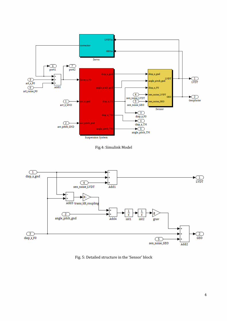
The Simulink model of IP control is shown in Fig. 4 and details of ‘Sensor’ and ‘Servo’ blocks are shown in

Figs. 5 and 6. The sensing part of the geophone becomes rather complicated to introduce the tilt sensitivity.

The sensitivity to the tilt becomes larger in low frequencies, and the conversion factor from the ground tilt to

the read-out displacement is written as (g/s2) [m/rad], where g is gravity constant and s is Laplace variable.

The ‘trans_tilt_coupling’ in Fig. 5 shows the translation-tilt coupling of the IP stage due to asymmetry in IP leg

lengths. The number is at most α~10-4 for 50 cm length IP.

The geophone signal and LVDT signal are blended in the servo and the blended signal is used for feedback

control. The blending filters are constructed so that the sum of two filters becomes unity. Detailed design of

the blending filters is shown in the next chapter.

4

Fig.4: Simulink Model

Fig. 5: Detailed structure in the ‘Sensor’ block

5

Fig. 6: Detailed structure in the ‘Servo’ block

2.4. Suspension Mechanical Response

Figs. 7-10 show frequency response of type-A SAS to various excitations. The IP stage becomes more

sensitive to the DC ground tilt when it is tuned at lower frequency. In the current design, the coupling factor

is ~1E2 [m/rad].

Fig. 7: Displacement transfer functions from ground translation to F0 and TM translation (red and blue lines).

The black curve shows the ratio of two curves.

6

Fig. 8: Transfer functions from ground tilt to F0 and TM translation.

Fig. 9: Transfer function from the ground /F0 translation to the test mass pitch rotation

7

Fig. 10: Transfer function from the top stage actuator to F0 translation

3. Simulation

3.1. Sensor Blending

Blending filters are derived from polynomial calculus. For example, 5th order blending filter is expressed as

follows:

5

0

5

0

4

0

23

0LP5

0

32

0

4

0

5

HP)(

510 ,

)(

105

ss

sssssH

ss

sssssH

, (1)

where s0 represents the blending angular frequency. Since the sum of two filters is unity, no phase rag would

occur at overlap frequency.

The blending filters used in the following simulation are based on the 5th order polynomial with blending

frequency at 40 mHz, but it also contains steeper cutoff in the low pass filter (for LVDT), with notch filters.

Their zero and pole lists are shown in Table 1.

8

High pass filter GAIN: 1

ZERO:

Frequency [Hz] 0 0 0.133

Q - 0.5 0.756

POLE:

Frequency [Hz] 0.04 0.04 0.04

Q - 0.5 0.5

Low pass filter GAIN: 0.1108

ZERO:

Frequency [Hz] 0.0126 0.197 0.302

Q 0.632 20 20

POLE:

Frequency [Hz] 0.04 0.04 0.04 0.197 0.4

Q - 0.5 0.5 2 -

Table 1: Zero/pole lists of blending filters. When the Q-value is not defined, it means single zero/pole

Fig. 11: Blending filter plots

9

3.2. Servo Filters

A simple PID filter with low pass cutoff (50 Hz) is used as a servo filter. Fig. 12 shows Bode plot of the servo

and Fig.13 shows open loop transfer function of the IP control.

Servo filter GAIN: 5E10

ZERO:

Frequency [Hz] 0.04

Q 0.5

POLE:

Frequency [Hz] 0 50 50

Q - - 0.5

Table 2: Zero/pole lists of servo filter

Fig. 12: Servo filter design

3.3. Tilt Coupling

In the following simulation, we assume no translation-tilt coupling in IP stage, i.e. α=0.

10

Fig. 13: Open loop transfer function

3.4. Close loop transfer functions

Figs. 14 and 15 show close-loop transfer function from ground motion to the test mass longitudinal

displacement. Sensitivity at 0.15-0.3 Hz is isolated more by inertial control, but the sensitivity to the tilt

below 0.2 Hz goes up due to the tilt sensitivity of geophone.

Fig. 14: Displacement transfer function from ground to TM, with and without control

11

Fig. 15: Transfer function from ground tilt to TM translation, with and without control

3.5. Noise Budget

Fig, 16 shows the noise contribution to the test mass displacement, and Fig.17 shows the comparison

between passive and active model. Note that they display the displacement spectrum of a single test mass,

and the differential arm length fluctuation can be calculated by multiplying a factor of √4 = 2 to the displayed

spectrum.

RMS displacement due to micro-seismic peak is suppressed by a factor of 3 with inertial controls. However,

low frequency (<0.1 Hz) fluctuation is enhanced due to glowing noise of geophone at low frequencies. Note

that the fluctuation due to geophone noise only affects RMS displacement of the mirror, while RMS velocity is

not affected so much.

Fig, 18 shows TM displacement noise from the top stage horizontal vibration of passive and active system.

Although the control enhances the high frequency test mass vibration, the vibration level above 10 Hz is well

below the target sensitivity. So, we don’t need to care about high frequency control noise.

12

Fig. 16: Noise contribution to test mass displacement

Fig. 17: Comparison of TM displacement noise between passive and active model. The dotted dark lines (with

“V” in the legend) show RMS velocity.

13

Fig. 18: Comparison of TM displacement noise between passive and active model at high frequencies

The obtained RMS displacement and velocity do not meet the requirement. In order to reach the required

RMS displacement or velocity:

Noise from inertial sensor electronics must be suppressed. One possibility is applying high pass filters

with steeper cutoff or larger cutoff frequency. Another possibility is using less noisy sensor at low

frequencies.

Vibration at micro-seismic peak must be suppressed by a factor of 3 more. One needs to decrease the

control gain of displacement sensor (LVDT) and increase the control gain of inertial sensor. That means

low pass filter with steeper cutoff or lower cutoff frequency is required, which contradicts the previous

problem mentioned above.

Noise contribution from the ground tilt is to be investigated. If one lowers the overlap frequency of two

sensors, tilt noise enhancement by inertial sensors might be a problem.

4. Additional Simulation

4.1. Increasing servo gain

In order to suppress the micro-seismic peak more, higher servo gain is tested. There exists ~60 degrees

phase margin at unity gain frequency and we still have a large room to increase the control gain. Here we try

10 times large control gain. Fig.19 shows the open loop transfer function.

14

Fig. 19: Open-loop transfer function with larger control gain

Fig, 20 shows noise budget in the case of higher control gain. In this servo design, however, the noise around

micro-seismic peak gets worse due to phase mismatch around the notch at 0.16 Hz. One may need to

compensate the phase in servo filters, which is under investigation.

15

Fig. 20: Noise contribution to TM displacement

4.2. Comparison with Normal Blending

Here we apply the same servo filter but different blending filters. The ‘new’ blending filters shown in Fig.21

are those used in the simulation above, and ‘old’ blending filters are simple filters constructed from eq. (1)

with 40 mHz blending. Fig.22 shows the comparison of TM displacement noise in two cases. The achieved

RMS displacement at micro seismic peak is much better in the case with notched blending filters.

Fig. 21: Blending filters

16

Fig. 22: Noise comparison

5. Conclusion and Future Works

One needs to improve the servo filters to achieve required RMS displacement and velocity. Just

increasing the control gain does not work, and it might be necessary to compensate the phase mismatch

due to a notch at 0.16 Hz in mechanical response.

The sensor noise of inertial sensor (geophone) is serious below 0.1 Hz and one might be necessary to

use inertial sensor with displacement readout, not with velocity readout like geophone.

Ground tilt noise should be taken into account to complete this work. Also the translation-tilt coupling of

the IP stage should be included.