Embed Size (px)
Citation preview
Stabilization of Inverted Pendulum Systems
David G. Aristoff
Department of Mathematics, University of Michigan
Abstract
This paper presents a condition that stabilizes a general invertedpendulum system (IPS) and outlines a control law for the coordinatedstabilization of several IPS’s. It is shown that a system of any numberof IPS’s is an SMC system, and relates the IPS concept to systems likethe inverted planar pendulum on a cart and the spherical pendulumon a puck.
1 Introduction
Most of this paper draws from the Method of Controlled Lagrangians inBloch, Leonard and Marsden [2000] and Bloch, Chang, Leonard and Mars-den [2000], hereafter referred to as [BLM] and [BCLM]. The graphs showingasymptotic stability were obtained by following energy methods outlined in[BCLM]. Kapitza [1951] analyzes a different method of stabilization.
2 Inverted Pendulum Systems
An n-inverted pendulum system (n-IPS) in <3 consists of point massesm0, m1, ..., mn with displacement vectors s,x1, ...,xn, respectively, in a givenfixed inertial frameOxyz. The system is subject to the constraints ‖s− x1‖ =d1 and ‖xi − xi+1‖ = di+1 for i = 1, ..., n− 1, where the di are constants.The point masses experience a gravitational potential. The system’s energyis
12m0s · s +
12
n∑
i=1
mixi · xi + V,
where V is the potential energy.
1
3 Generalized Coordinates and Lagrangian
Let {e1, e2, e3} be an orthonormal basis for the space frame Oxyz. Write
s =3∑
i=1
siei,x1 =3∑
i=1
x1iei, ...,xn =3∑
i=1
xniei
so that one has Cartesian coordinates (s1, s2, s3, x11, x12, x13, ..., xn1, xn2, xn3)describing the position of the IPS. Obtain generalized coordinates(s1, s2, s3, ϕ1, ψ1, ..., ϕn, ψn) by putting the (i+ 1)th point mass in sphericalcoordinates relative to the position of the ith mass:
xi − xi−1 = di cosϕi sinψie1 + di sinϕi sinψie2 + di cosψie3
x1 − s = d1 cosϕ1 sinψ1e1 + d1 sinϕ1 sinψ1e2 + d1 cosψ1e3
The angles ϕi and ψi are measured in the inertial frame with respect to thebasis {e1, e2, e3}. It is clear that the configuration space Q is <3 × S2 ×... × S2 (there are n + 1 factors). Let ai be a unit vector in the directionof xi − xi−1 and suppose the potential energy is given by gravity times thesum of the products of the point masses m0, m1, ..., mn and the componentsin the direction of e3 of the corresponding displacement vectors s,x1, ...,xn.That is, let V = gm0s · e3 + gm1x1 · e3 + ...+ gmnxn · e3. The Lagrangian,in this case the kinetic minus potential energy, is then
L =n∑
i,j=1
(12αijdidj ai · aj + αidiai · s +
12α0s · s− gαidiai · e3 − gα0s · e3
)
where αi =n∑k=i
mk and αij =n∑
k=max(i,j)
mk. Let fα (x) =
{cosx, α = 0sinx, α = 1
}
and let Pαβγδij = fα (ϕi) fβ (ψi) fγ (ϕj) f δ (ψj), Qαβi = fα (ϕi) fβ (ψi), R
αβij =
fα (ψi) fβ (ψj), Tαi = fα (ψi). Now
L =
n∑i,j=1
12αijdidj
(P 1111ij + P 0101
ij
)ϕiϕj + 1
2αijdidj(R11ij + P 0000
ij + P 1010ij
)ψiψj
+αijdidj(P 0110ij − P 1100
ij
)ϕiψj − αidiQ
11i ϕis1 + αidiQ
00i ψis1
+αidiQ01i ϕis2 + αidiQ
10i ψis2 − αidiT
1i ψis3
+12α0s
21 + 1
2α0s22 + 1
2α0s23 − gαidiT
0i − gα0s3
2
Note that the dynamics are invariant to translations of s1 and s2, since theLagrangian does not depend on these variables. Let the additive group <2
act on the configuration space, where the action of (a, b) ∈ <2 on<3 × S2 × ...× S2 is given by
(a, b) · (s1, s2, s3, ϕ1, ψ1, ..., ϕn, ψn) = (s1 + a, s2 + b, s3, ϕ1, ψ1, ..., ϕn, ψn)
so that G is a symmetry group. Note that the shape space is<× S2 × ...× S2. The Euler-Lagrange equations of motion for the n-IPSare
εϕi (L) =
n∑j=1
αijdidj(P 1111ij + P 0101
ij
)ϕj + αijdidj
(P 0110ij − P 1100
ij
)ψj
+αijdidj(P 1101ij − P 0111
ij
)ϕ2j + αijdidj
(P 1101ij − P 0111
ij
)ψ2j
+2αijdidj(P 0100ij + P 1110
ij
)ϕjψj − αidiQ
11i s1 + αidiQ
01i s2
= 0
εψi (L) =
n∑j=1
αijdidj(R11i + P 0000
ij + P 1010ij
)ψj + αijdidj
(P 1001ij − P 0011
ij
)ϕj
+αijdidj(R10i − P 0001
ij − P 1011ij
)ψ2j + αijdidj
(−P 0001
ij − P 1011ij
)ϕ2j
+2αijdidj(P 1000ij − P 0010
ij
)ϕjψj + αidikQ
00i s1 + αidiQ
10i s2
−αidiT 1i s3 − gαidiT
1i
= 0
εs1 (L) =n∑j=1
(α0s1 − αjdjQ
11j ϕj + αjdjQ
00j ψj
−αjdjQ01j ϕ
2j − αjdjQ
01j ψ
2j − 2αjdjQ10
j ϕjψj
)= 0
εs2 (L) =n∑j=1
(α0s2 + αjdjQ
01j ϕj + αjdjQ
10j ψj
−αjdjQ11j ϕ
2j − αjdjQ
11j ψ
2j + 2αjdjQ00
j ϕjψj
)= 0
εs3 (L) =n∑j=1
(α0s3 − αjdjT
1j ψj − αjdjT
0j ψ
2j + gα0
)= 0
where εx is the Euler-Lagrange operator defined by εx (L) = ddt∂L∂x − ∂L
∂x .
3
4 Stabilization
The goal of this paper is to stabilize the IPS about the upright equilibriaψ1 = ψ1 = ... = ψn = ψn = 0, ϕ1 = ... = ϕn = 0, s1 = ξ1, s2 = ξ2, s3 = 0,where the ξi are constants, by letting <2 act on the configuration space asdiscussed in the last section. That is, the point mass m0 will be directed tomove in a plane parallel to the one spanned by e1 and e2 so that the othermasses will be balanced near the upright position. Interestingly, it has beenshown that a 1-IPS may be stabilized by moving the massm0 vertically (i.e.,in the subspace spanned by e3). See, for example, Kapitza [1951].
This paper will apply the Method of Controlled Lagrangians from Bloch,Leonard and Marsden [2000] (hereafter called [BLM]) to stabilize the system.Note that the upright equilibria described above are relative equilibria, sincethey are solutions of the Euler-Lagrange equations that lie inside <2-orbits.See [BLM].
In the Method of Controlled Lagrangians, each vector v in TQ is decom-posed into two components: V er (v), a vector tangent to the orbits of theG-action, and Hor (v), a vector in the metric orthogonal space to the spaceof vertical vectors. The components are called the vertical and horizontalparts, respectively, of v. One may think of the vertical part of a tangentvector as a piece in the <2 (group) direction. The horizontal part can bevisualized as a piece in the S2 × ...× S2 (shape) direction.
This problem will require kinetic shaping only (as opposed to kinetic andpotential shaping; for a reference, see Bloch, Chang, Leonard and Marsden[2001]) since the group <2 acts only on symmetry variables. The kineticenergy will be reshaped with a new choice of horizontal space, Horτ , and anadjustment by a scalar factor, σ, of the metric acting on horizontal vectors.
The Controlled Lagrangian Lτ,σ incorporates the new kinetic energy.The goal is to match the Euler-Lagrange equations corresponding to theControlled Lagrangian (CL) with the controlled L-equations, called the con-trolled cart (CC) equations, which are the Euler-Lagrange equations for Lwith controls affecting the symmetry variables. The Simplified MatchingConditions (SMC) of [BLM] are sufficient to guarantee the existence of pa-rameters τ and σ such that the CC and CL equations match. Hence ifthe SMC hold, the Energy-Momentum Method can be used to check stabil-ity, since the CL system is Lagrangian (i.e., it satisfies the Euler-Lagrangeequations). For a reference on the Energy-Momentum Method, see Bloch,Marsden and Zenkov [1998].
Note that since m0 will be moved only in the plane spanned by e1 and e2,
4
the (nonsymmetry) position variable s3 will remain constant. Hence withoutloss of generality, suppose s3 ≡ 0. (If s3 ≡ c, c 6= 0, then the potentialenergy is changed by the constant factor gα0c and the kinetic energy isunchanged, so the Lagrangian differs by a constant, which vanishes in theEuler-Lagrange equations.) In light of this, the SMC for kinetic shapinghold, since α0 is a constant and
∂(−Q11i )
∂ϕi= −Q01
i =∂(Q00
i )∂ψi
,∂(−Q11
i )∂ψi
= −Q10i =
∂(Q00i )
∂ϕi,
∂(Q01i )
∂ϕi= −Q11
i =∂(Q10
i )∂ψi
,∂(Q01
i )∂ψi
= Q00i =
∂(Q10i )
∂ϕi,
∂(−Q11i )
∂ϕj=
∂(−Q11i )
∂ψj=
∂(Q00i )
∂ϕj=
∂(Q00i )
∂ψj=
∂(Q01i )
∂ϕj=
∂(Q01i )
∂ψj=
∂(Q10i )
∂ϕj=
∂(Q01i )
∂ψj= 0
for j 6= i. See [BLM]. The conditions define τ and σ, producing controllaws uconsj and a CL Lτ,σ such that the systems
εϕi (L) = εψi (L) = 0, i = 1, ..., n,εs1 (L) = u1, εs2 (L) = u2
and
εϕi (Lτ,σ) = εψi (Lτ,σ) = εs1 (Lτ,σ) = εs2 (Lτ,σ) = 0, i = 1, ..., n
are equivalent. See Theorem 3.2, [BLM]. Following [BLM], the controls are
ucons1 = −n∑i=1
ddt
(1σαidiQ
11i ϕi − 1
σαidiQ00i ψi
)
ucons2 = −n∑i=1
ddt
(− 1σαidiQ
01i ϕi − 1
σαidiQ10i ψi
)
and the CL is
5
Lτ,σ =
n∑i,j=1
12αijdidj
(P 1111ij + P 0101
ij
)ϕiϕj
+12αijdidj
(R11ij + P 0000
ij + P 1010ij
)ψiψj
+αijdidj(P 0110ij − P 1100
ij
)ϕiψj
+αidi(Q00i ψi − Q11
i ϕi)(s1 + 1
σαj
α0djQ
11j ϕj − 1
σαj
α0djQ
00j ψj
)
+αidi(Q01i ϕi +Q10
i ψi)(s2 − 1
σαj
α0djQ
01j ϕj − 1
σαj
α0djQ
10j ψj
)
−αidiT 1i ψis3
+12α0
(s1 + 1
σαiα0diQ
11i ϕi − 1
σαiα0diQ
00i ψi
)2
+12α0
(s2 − 1
σαiα0diQ
01i ϕi − 1
σαiα0diQ
10i ψi
)2
+12α0s3
+12
(1σαiα0diQ
11i ϕi − 1
σαiα0diQ
00i ψi
)(−αjdjQ11
j ϕj + αjdjQ00j ψj
)
+12
(− 1σαiα0diQ
01i ϕi − 1
σαiα0diQ
10i ψi
)(αjdjQ
01j ϕj + αjdjQ
10j ψj
)
−gαidiT 0i − gα0s3
5 Stability
In this section it will become apparent that it is difficult to stabilize a gen-eral n-IPS for n ≥ 2 using the Method of Controlled Lagrangians. If thepoint masses m1, ..., mn are constrained to move in a plane (by, for example,forcing ϕ1 = ... = ϕn = c ∈ [0, 2π] at any time t), however, there is a nicecondition for stabilization.
One may check that the Euler-Lagrange equations for the CL match theCC equations, and in fact, the systems corresponding to the LagrangiansL and Lτ,σ have the same relative equilibria. See Prop. 3.3, [BLM]. Hencethe CC system is Lyapunov stable at the relative equilibria ψ1 = ψ1 = ... =ψn = ψn = 0, ϕ1 = ... = ϕn = 0, s1 = ξ1, s2 = ξ2, s3 = 0 if the secondvariation of E = KEτ + V is definite there, where KEτ is the horτ kineticenergy and V is the amended potential as defined in [BLM].
Let EQ be the set of vectors in TQ satisfying ψ1 = ψ1 = ... = ψn = ψn =0, ϕ1 = ... = ˙ ϕn = 0, ϕ1 = ... = ϕn, s1 = ξ1, s2 = ξ2, and s3 = 0, where theξi are constants. Think of EQ as the set of upright relative equilibria for an-IPS with point masses constrained to move in a plane. Let Γi = −gαidi ,and for i ≤ j , let βij =
(αj +
(1σ − 1
)αiαj
α0
)didj . Let
6
Bk =
2β11 β12 · · · β1k
β12 2β22...
.... . .
...β1k · · · · · · 2βkk
, C =
Γ1 0 · · · 0
0 Γ2...
.... . .
...0 · · · · · · Γn
,
D =
δϕ1...
δϕn
, E =
δϕ1...
δϕn
, X =
(Bn2 00 C
)
Lemma 1.1. The system εϕi(L) = εψi(L) = 0, εs1(L) = ucons1 andεs2(L) = ucons2 is stable at the relative equilibrium v ∈ EQ if the matrix Xis definite.
Proof . From [BLM], the system is stable at a relative equilibrium if thesecond variation of Eτ , the sum of the τ -horizontal energy and theamended potential energy, is definite there. Following formulas (3.13) and(3.20) from [BLM], the τ -horizontal energy is
12
n∑i,j=1
αijdidj(P 1111ij + P 0101
ij
)
+(−αidiQ11
i
) (− 1σα0
+ 1α0
)(−αjdjQ11
j
)
+(αidiQ
01i
) (− 1σα0
+ 1α0
) (αjdjQ
01j
)
ϕiϕj
+12
n∑i,j=1
αijdidj(R11ij + P 0000
ij + P 1010ij
)
+(αidiQ
00i
) (− 1σα0
+ 1α0
)(αjdjQ
00j
)
+(αidiQ
10i
) (− 1σα0
+ 1α0
)(αjdjQ
10j
)
ψiψj
+12
n∑i,j=1
αijdidj(P 0110ij − P 1100
ij
)
+(−αidiQ11
i
) (− 1σα0
+ 1α0
)(αjdjQ
00j
)
+(αidiQ
01i
) (− 1σα0
+ 1α0
)(αjdjQ
01j
)
ϕiψj
Noting that Qαβi Qγδj = P
αβγδij and Tαi T
βj = R
αβij , this becomes
12
n∑i,j=1
12
(P 1111ij + P 0101
ij
)(αijdidj +
(1σ − 1
)αiαj
α0
)ϕiϕj
+12
(R11ij + P 0000
ij + P 1010ij
)(αijdidj) ψiψj
+12
(P 0000ij + P 1010
ij
)(1σ − 1
)(αiαj
α0
)ψiψj
+12
(P 0110ij − P 1100
ij
)(αijdidj +
(1σ − 1
)αiαj
α0
)ϕiψj
At any point v in EQ , the second variation of this is
7
12
n∑i,j=1
(αijdidj +
(1σ − 1
)αiαj
α0
)δψiδψj
Note that the second variation at a relative equilibrium point notsatisfying ϕ1 = ... = ϕn depends on these angles; this proof requires thatthe angles be the same. See Remark 1. Following formula (3.19) from[BLM], the amended potential energy is
n∑i=1
(gαidiT
0i + 1
2α0
(ξ21 + ξ22
))
where the ξi are the components of s at the equilibrium. The second termin the parentheses is a constant, so it vanishes in the variations. It followsthat the second variation of the amended potential at any point v in EQ is
−n∑i=1
gαidi (δψi)2
Hence δ2E∣∣EQ is
(DE
)TX
(DE
)
which is definite if and only if X is a definite matrix. This completes theproof.
Theorem 1.1. The system εϕi(L) = εψi(L) = 0, εs1(L) = ucons1 andεs2(L) = ucons2 is stable at the relative equilibrium v ∈ EQ if − 1
σ >α0−α1α1
.
Proof . Note that since Γi = −gαidi < 0 for i = 1, ..., n,X is definite if andonly if Bn is negative definite.
Let
Yk =
2 1 · · · 1
1 2...
.... . .
...1 . . . · · · 2
︸ ︷︷ ︸k×k
, βij =
{2βii, i = j
βij , i 6= j
},
f (i) =(1 +
(1σ − 1
)αiα0
)di, g (j) = αjdj
8
Denote the group of permutations of {1, ..., k} by Sk. For anyγ ∈ Sk, k = 1, ..., n, let Okγ =
{i ∈ {1, ..., k} : γ (i) = i
}and define
ηk : Sk → {1, ..., k} by ηk (γ) =∣∣∣Okγ
∣∣∣. Note that
det (Yk) = det
I +
0 · · · 0 −1...
. . ....
...0 · · · 0 −11 · · · 1 1
︸ ︷︷ ︸k×k
= k + 1
Now
det (Bk) =∑γ∈Sk
sgn (γ) β1γ(1)...βkγ(k)
=∑γ∈Sk
2ηk(γ)sgn (γ)β1γ(1)...βkγ(k)
=∑γ∈Sk
2ηk(γ)sgn (γ) f (1) g (γ (1)) ...f (k) g (γ (k))
=∑γ∈Sk
2ηk(γ)sgn (γ) f (1) g (1) ...f (k) g (k)
=∑γ∈Sk
2ηk(γ)sgn (γ)β11...βkk
= β11...βkk
(∑γ∈Sk
2ηk(γ)sgn (γ)
)
= β11...βkk (det (Yk))= (k + 1)β11...βkk
Hence Bn is negative definite if and only if βii < 0 for i = 1, ..., n. Notethat the latter is true
⇔(αi −
(1 − 1
σ
)α2
iα0
)di
2< 0, i = 1, ..., n
⇔ − 1σ >
α0αi
− 1, i = 1, ..., n⇔ − 1
σ >α0α1
− 1 = α0−α1α1
So X is negative definite if and only if − 1σ >
α0−α1α1
. By the lemma, thesystem is stable if σ satisfies this condition. This completes the proof. Seefigs. 1a, 1b.
9
6 Stability of Planar IPS
The set of relative equilibria EQ is rather artificial, since one cannotexpect ϕ1 = ... = ϕn near an upright equilibrium point. Some newdefinitions are therefore in order.
Let Qθ be the set of vectors in Q satisfying ϕ1 = ... = ϕn = θ ∈ [0, 2π], andlet TQθ be the corresponding tangent space. Let Lθ be the restriction ofthe Lagrangian to TQθ. That is, given v ∈ TQθ, let Lθ (v) = L (v). ThenLθ is an SMC system (since L is); let uθ1, u
θ2 and Lθ,τ,σ be the
corresponding controls and CL, respectively, obtained by applying theMethod of Controlled Lagrangians. Let EQθ be the set of vectors in TQθsatisfying ψ1 = ψ1 = ... = ψn = ψn = 0 and s1 = ξ1, s2 = ξ2, where the ξiare constants.
Corollary 1.1. The system εψ1(Lθ) = ... = εψn(Lθ) = 0, εs1(Lθ) = uθ1 andεs2(Lθ) = uθ2 is stable at the relative equilibrium v ∈ EQθ if − 1
σ >α0−α1α1
.
Proof . At any point v ∈ EQθ, the second variation of Eθ (the sum of thehorθτ kinetic energy and amended potential energy), is the same as thesecond variation of E as defined in the lemma. Hence the proof ofTheorem 1.1 holds, confirming the condition given above.
7 Remarks
Rmk. 1. Note that the second variation of the horτ kinetic energy at arelative equilibrium point not satisfying ϕ1 = ... = ϕn is
n∑
i,j=1
(cosϕi cosϕj + sinϕi sinϕj)(αijdidj +
(1σ− 1
)αiαjα0
)δψiδψj
Rmk. 2. Note that the proof of Theorem 1.1 holds for the special case ofthe 1-IPS mith mass m0 moving in the plane and m1 moving in space. Seethe section on the spherical pendulum on a puck from [BLM]; the stabilitycondition of Theorem 1.1 matches the condition given in that paper.
Rmk. 3. The 1-IPS constrained to move in a plane is the invertedpendulum on a cart, also from [BLM]. The stability condition given inTheorem 1.1 is consistent with the conditions presented in that paper.
10
Rmk. 3. Notice that the stability condition is equivalent to
− 1σ>
m0n∑i=1
mi
.
8 Asymptotic Stabilization and Full Phase Space
Stabilizaton
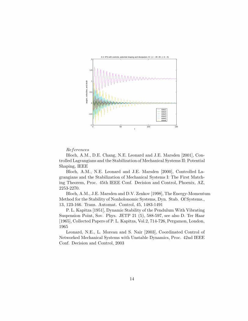
Given stability in the sense of Lyapunov (as achieved in section 6), asymp-totic stabilization can be relatively easily achieved by using energy methodsoutlined, for example, in [BLM]. Complete phase space stabilization requiresa bit more work, but a general method can be found in Bloch, Chang,Leonard and Marsden [2001]. See figs 2a, 2b, 3a, and 3b.
9 Figures
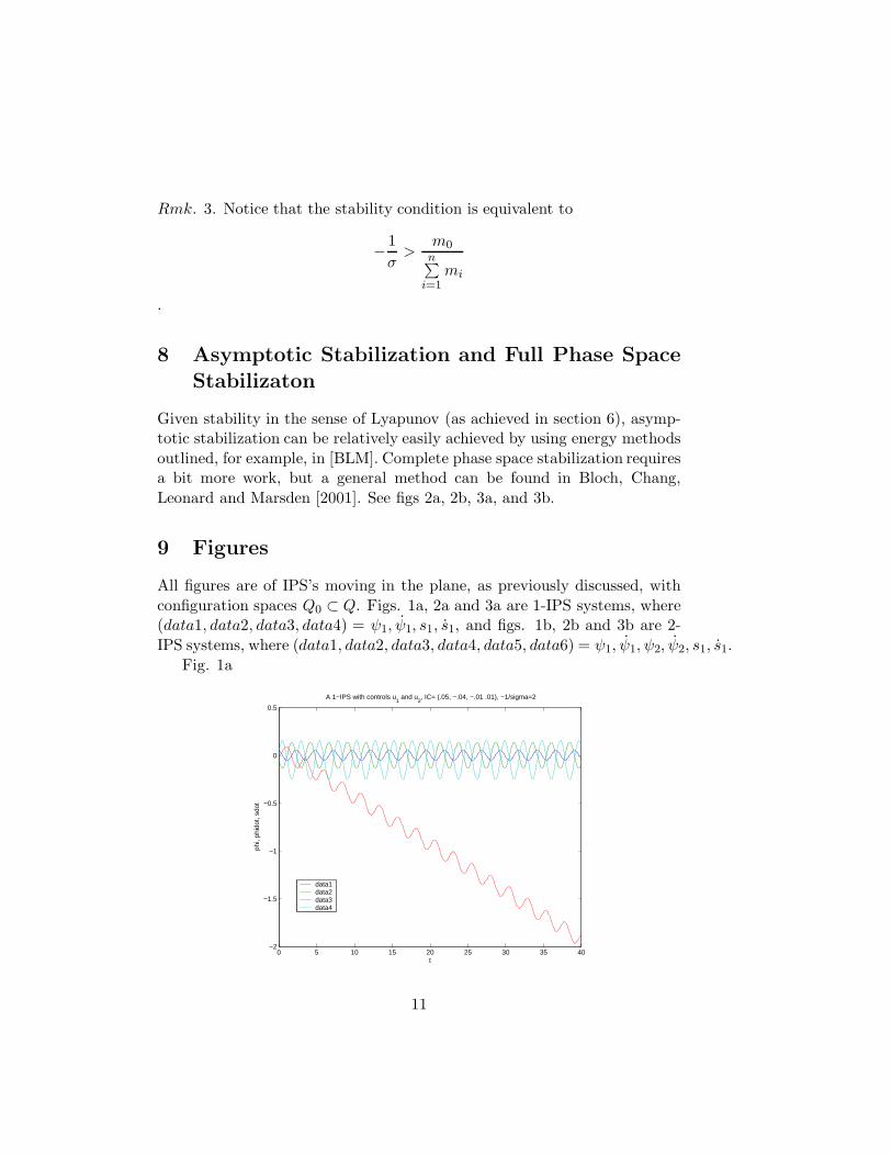
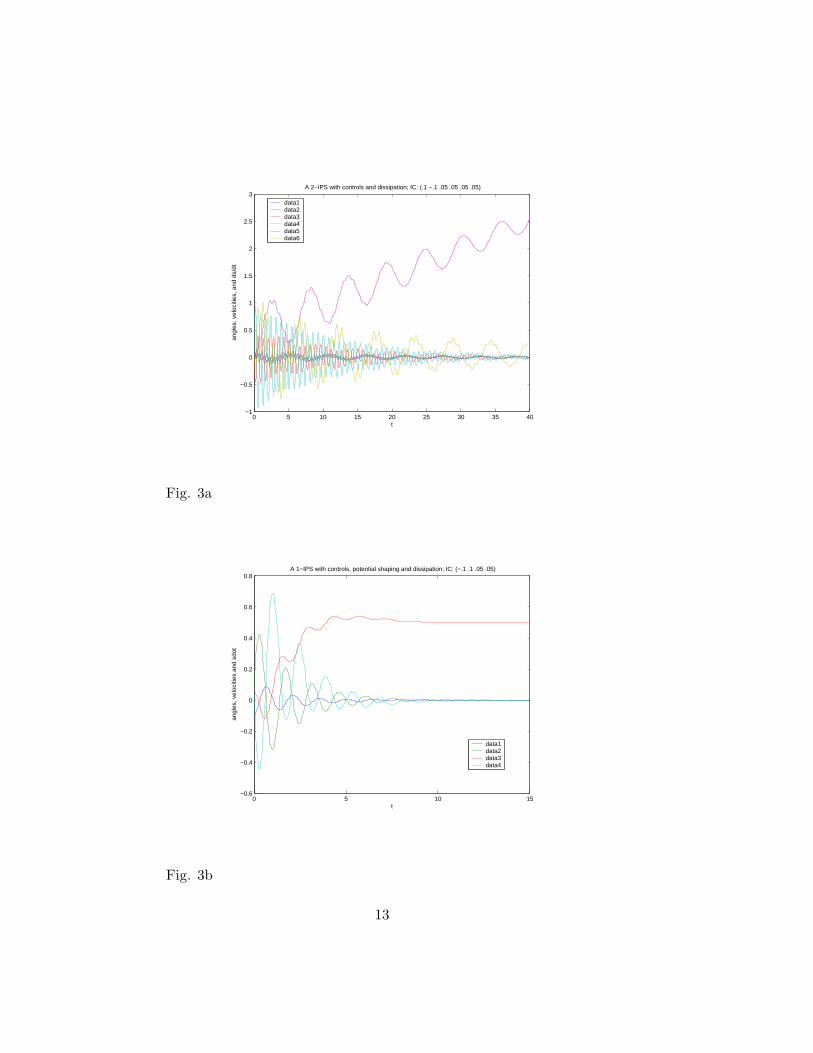
All figures are of IPS’s moving in the plane, as previously discussed, withconfiguration spaces Q0 ⊂ Q. Figs. 1a, 2a and 3a are 1-IPS systems, where(data1, data2, data3, data4) = ψ1, ψ1, s1, s1, and figs. 1b, 2b and 3b are 2-IPS systems, where (data1, data2, data3, data4, data5, data6) = ψ1, ψ1, ψ2, ψ2, s1, s1.
Fig. 1a
0 5 10 15 20 25 30 35 40−2
−1.5
−1
−0.5
0
0.5
t
phi,
phid
ot, s
dot
A 1−IPS with controls u1 and u
2, IC= (.05, −.04, −.01 .01), −1/sigma=2
data1data2data3data4
11
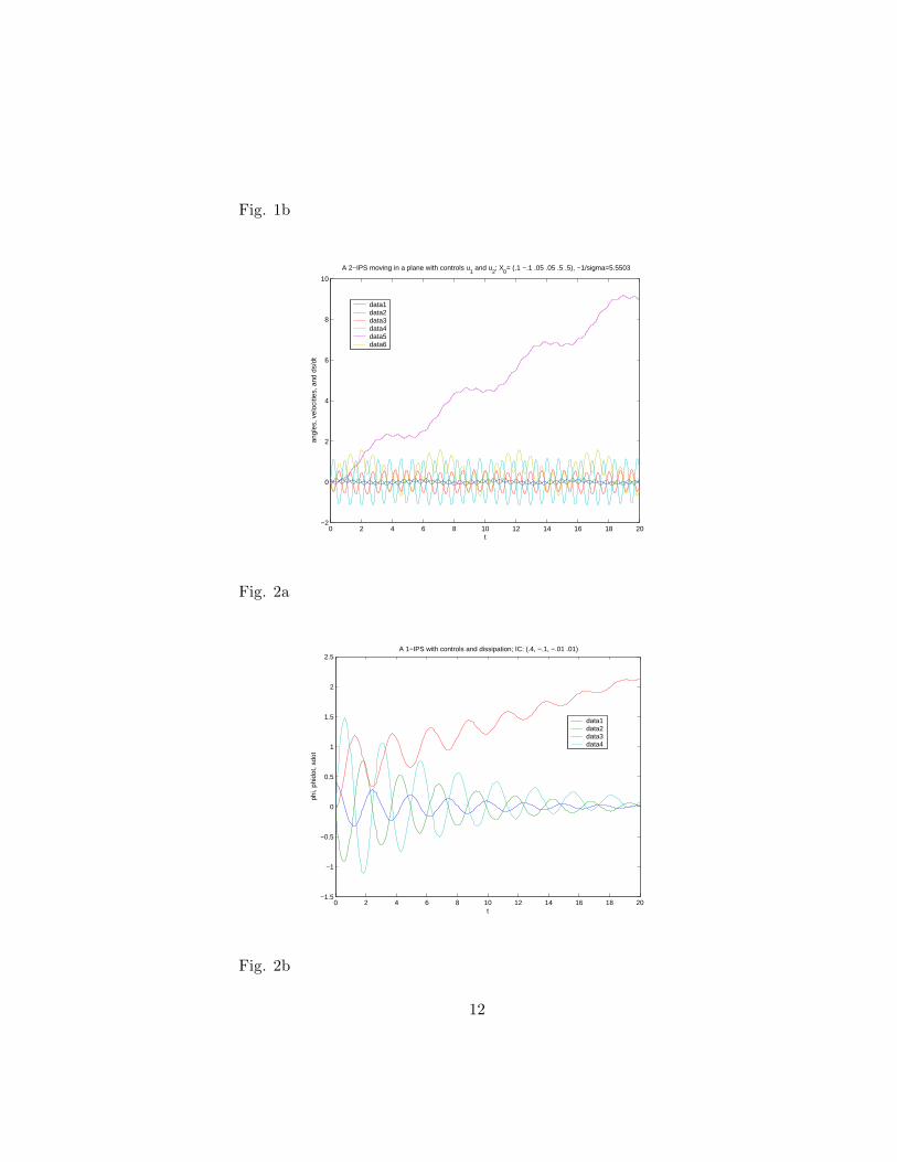
Fig. 1b
0 2 4 6 8 10 12 14 16 18 20−2
0
2
4
6
8
10
t
angl
es, v
eloc
ities
, and
ds/
dt
A 2−IPS moving in a plane with controls u1 and u
2; X
0= (.1 −.1 .05 .05 .5 .5), −1/sigma=5.5503
data1data2data3data4data5data6
Fig. 2a
0 2 4 6 8 10 12 14 16 18 20−1.5
−1
−0.5
0
0.5
1
1.5
2
2.5
t
phi,
phid
ot, s
dot
A 1−IPS with controls and dissipation; IC: (.4, −.1, −.01 .01)
data1data2data3data4
Fig. 2b
12
0 5 10 15 20 25 30 35 40−1
−0.5
0
0.5
1
1.5
2
2.5
3
t
angl
es, v
eloc
ities
, and
ds/
dt
A 2−IPS with controls and dissipation; IC: (.1 −.1 .05 .05 .05 .05)
data1data2data3data4data5data6
Fig. 3a
0 5 10 15−0.6
−0.4
−0.2
0
0.2
0.4
0.6
0.8
t
angl
es, v
eloc
ities
and
sdo
t
A 1−IPS with controls, potential shaping and dissipation; IC: (−.1 .1 .05 .05)
data1data2data3data4
Fig. 3b
13
0 50 100 150−1
−0.5
0
0.5
1
1.5
2
t
angl
es, v
eloc
ities
, and
ds/
dt
A 2−IPS with controls, potential shaping and dissipation; IC: (.1 −.05 .05 .1 .5 −.5)
data1data2data3data4data5data6
ReferencesBloch, A.M., D.E. Chang, N.E. Leonard and J.E. Marsden [2001], Con-
trolled Lagrangians and the Stabilization of Mechanical Systems II: PotentialShaping, IEEE
Bloch, A.M., N.E. Leonard and J.E. Marsden [2000], Controlled La-grangians and the Stabilization of Mechanical Systems I: The First Match-ing Theorem, Proc. 45th IEEE Conf. Decision and Control, Phoenix, AZ,2253-2270.
Bloch, A.M., J.E. Marsden and D.V. Zenkov [1998], The Energy-MomentumMethod for the Stability of Nonholonomic Systems, Dyn. Stab. Of Systems.,13, 123-166. Trans. Automat. Control, 45, 1483-1491
P. L. Kapitza [1951], Dynamic Stability of the Pendulum With VibratingSuspension Point, Sov. Phys. JETP 21 (5), 588-597, see also D. Ter Haar[1965], Collected Papers of P. L. Kapitza, Vol.2, 714-726, Pergamon, London,1965
Leonard, N.E., L. Moreau and S. Nair [2003], Coordinated Control ofNetworked Mechanical Systems with Unstable Dynamics, Proc. 42nd IEEEConf. Decision and Control, 2003
14


![Inverted Pendulum [Final]](https://img.dokumen.tips/doc/110x75/58904db31a28abcb668bcda8/inverted-pendulum-final.jpg)