Embed Size (px)
Citation preview

Control of Nonlinear Distributed Parameter Systems
edited byGoong Chen, Texas A&M University, College Station, Texas
Irena Lasiecka, University of Virginia, Charlottesville, VirginiaJianxin Zhou, Texas A&M University, College Station, Texas

iii
Preface
This volume is an outgrowth of the conference “Advances in Control ofNonlinear Distributed Parameter Systems”, held on October 22-23, 1999, atTexas A&M University, College Station, Texas. The conference was jointlysponsored by the National Science Foundation (NSF), The Institute of Math-ematics and Its Applications (IMA) and Texas A&M University. Fifty-fiveresearchers attended and twenty-six talks were delivered during the two-dayevent. Ten papers in this volume were written by those conference speakers.To further broaden the scope and appeal of this volume, we have invited sevenadditional papers from experts working in this field. Thus, a total of seventeenpapers have constituted the volume.
The mathematical theory of control is highly interdisciplinary—it isa part of applied mathematics serving perhaps the most important linkbetween mathematics and technology: complex systems in aerospace, civiland mechanical engineering must be controlled in order to achieve designatedmission or operational requirements. Many ultra-modern electronic andoptical devices are also designed for and dedicated to the purpose of actingas control mechanisms and media, i.e., actuators and sensors. Most of thosedevices are inherently nonlinear. The strong interest in mathematical con-trol problems among mathematicians and engineers alike can be witnessed inthe large number of papers published in the various journals of IEEE and SIAM.
Even though steady progress has been made in the overall study of themathematics of control, and wider and wider applications to new problemshave been found, the leading edge of the field, as a mathematical subject, isindisputably the area of control of distributed parameter systems (DPS). Thisarea concerns investigation of the control laws, stability and optimization ofsystems and feedback syntheses for systems whose states are spatially and/ortemporally distributed and whose governing equations are partial differentialor functional (typically time delay) equations. Studies in the area also includethe associated questions of modelling, identification and estimation, analysisand design, computation and visualization, etc., of DPS. Rapid progress hasoccurred in this area since its inception during the 1960’s and its initial burstof growth in the 1970’s.
After nearly three decades of research, though many interesting questionsremain open, control theory for linear DPS has attained a certain level ofmaturity. The momentum of DPS research is now visibly moving towardthe study of control of nonlinear partial differential equations. NonlinearDPS (NDPS) are very much model-dependent . Since comprehensive, unifiedtheories are virtually nonexistent, research opportunities and challenges are

iv
extraordinarily numerous. Very substantial payoffs from the study of controland optimization of wide-ranging, application-driven nonlinear DPS in variousareas of high technology may be expected to yield a substantial payoff throughoperational economies and enhanced system performance. We hope the presentvolume will stimulate active development of the mathematical theory in thiscritically important area.
Two major influences are driving the recent sharp surge of interest in controlof nonlinear distributed parameter systems:
(A) Advances in “smart” materials, active actuators and sen-sors, microelectromechanical systems (MEMS), etc.
Existing advanced, or “smart” materials largely consist of sophisticatedlaminates incorporating specialized layers in an overall matrix form; theyare fabricated to achieve a variety of desirable properties. Actuators and/orsensors consisting of piezoelectric/piezoceramic, opto-thermo-electric materialsor microprocessors can be bonded to external surfaces or embedded within thelayered structure itself. The response of such individual components is totallynonlinear, resulting in an overall system of nonlinear partial differential equa-tions as the operative mathematical model. For example, aircraft propellersand helicopter rotor blades may be designed so that varying pitch is achieved bytorsional actuation within the blade itself rather than by a mechanically articu-lated mechanism at the point where the blades are mounted. Another exampleconcerns active noise suppression in aircraft cabins. This is achieved by meansof actuator panels in the cabin walls, acting to achieve cancellation of highamplitude noise signals propagated through the fuselage. Many more examplesof ultra-modern micromachined elastic structures in diverse applications maybe found in a large number of new technical journals. The complete list ofnonlinear distributed parameter systems finding applications in the area of ad-vanced materials is much too long for us to cover in any representative way here.
(B) Advances in nonlinear PDEs and dynamical systems
The existing, now almost classical, theory of control of linear DPS is ofrather limited use in the nonlinear arena. New nonlinear methodology forcontrol, stabilization and optimization needs to be developed for such systems.During the past thirty years, dramatic breakthroughs in theory and methodsfor nonlinear PDEs have been made, including Lax’s entropy solution andGlimm’s method for hyperbolic conservation laws, The Mountain Pass Lemmaof Ambrosetti and Rabinowitz, the method of viscosity solutions, Hopfbifurcation phenomena in infinite dimensional spaces studied by Crandall andRabinowitz,. . . , enabling researchers to treat an increasing number of genuinely

v
nonlinear PDEs with confidence. These equations, or systems of equationsoften have unstable, multiple solutions, depending on the geometry of thedomain – a totally bewildering situation prior to recent developments. Theemergence of the new field of dynamical systems and chaos has likewise shiftedthe focus of attention from the classical qualitative theory of ODEs and PDEsto that of fractals, strange attractors, randomness, and their manipulations,control and applications—these are some of the most intensively investigatedtopics in the general scientific community at the present time.
Both exogenous and endogenous factors, i.e., (A) and (B), respectively,above, are simultaneously at work, enriching and propelling the study ofcontrol of nonlinear distributed parameter systems and cross-fertilizing otherintimately allied disciplines. These synergistic effects amply testify to thetimeliness of the publication of this volume.
The chapters in this volume cover interests in various aspects of NDPS.For example, the paper by Seidman and Antman is related to Category (A)above. The two papers by Ding and by Li and Zhou involve the applicationof the Mountain Pass Lemma and are thus more associated with Category(B). The paper by Chen, Huang, Juang and Ma studying chaotic phenomenadue to nonlinear boundary conditions has overlapping interests in both (A)and (B). We hope the wide range of topics in these, and the other papers notexplicitly cited here, will provide a useful reference for the study of nonlineardistributed parameter systems and stimulate further interest and research inthis important area.
We thank all the contributing authors for their work and and their patiencewith repetitive revisions. We are grateful to Dr. Deborah Lockhart at NSF,Professor Willard Miller, Jr. of IMA, and Professor Richard E. Ewing, Dean ofCollege of Science at Texas A&M University, for the financial support to theconference. Finally, we thank Ms. Maria Allegra and Helen Paisner at MarcelDekker and Professor M. Zuhair Nashed of the University of Delaware for theirkind assistance in expediting the editorial and publication process.
Goong Chen and Jianxin ZhouCollege Station, Texas
Irena LasieckaCharlottesville, Virginia

vi
Dedicated to
Professor David L. Russell
on the Occasion of his 60th Birthday

Contents vii
Preface iii
1. Shape Sensitivity Analysis in Hyperbolic Problems with nonSmooth DomainsJohn Cagnol and J. Paul Zolesio 1
2. Unbounded Growth of Total Variations of Snapshots of the 1DLinear Wave Equation due to the Chaotic Behavior of Iteratesof Composite Nonlinear Boundary Reflection RelationsGoong Chen, Tingwen. Huang, Jong Juang and Daowei Ma 15
3. Velocity method and Courant metric topologies in shapeanalysis of partial differential equationsMichel Delfour and J. Pual Zolesio 45
4. Nonlinear Periodic Oscillations In Suspension BridgesZhonghai Ding 69
5. Canonical Dual Control for Nonconvex Distributed-ParameterSystems: Theory and MethodDavid Y. Gao 85
6. Carleman estimate for a parabolic equation in a Sobolev spaceof negative order and their applicationsOleg Imanuvilev and Masahiro Yamamoto 113
7. Bilinear control for global controllability of the semilinearparabolic equations with superlinear termsAlexander Khapalov 139
8. A Nonoverlapping Domain Decomposition for Optimal Bound-ary Control of the Dynamic Maxwell SystemJohn E. Lagnese 157
9. Boundary Stabilizibility of a Nonlinear Structural AcousticModel Including Thermoelastic EffectsCatherine Lebiedzik 177
10. On Modelling, Analysis and Simulation of Optimal Con-trol Problems for Dynamic Networks of Euler-Bernoulli-andRayleigh-beamsGuenter Leugering and Wigand Rathman 199

viii Contents
11. Local Characterizations of Saddle Points and Their MorseIndicesYongxin Li and Jianxin Zhou 233
12. Static Buckling in a Supported Nonlinear Elastic BeamDavid Russell and Luther White 253
13. Optimal control of a nonlinearly viscoelastic rodThomas Seidman and Stuart Antman 273
14. Mathematical Modeling and Analysis for Robotic ControlSze-Kai Tsui 285
15. Optimal Control and Synthesis of Nonlinear Infinite Dimen-sional SystemsYuncheng You 299
16. Forced Oscillation of The Korteweg-De Vries-Burgers Equa-tion and Its StabilityBingyu Zhang 337

Shape Sensitivity Analysis in Hyperbolic Problems
with non Smooth Domains
John Cagnol1, Universite Leonard de Vinci, FST, DER-CS, 92916 Paris LaDefense Cedex, France, E-mail: [email protected] Zolesio, CNRS, Ecole des Mines de Paris, 06902 Sophia AntipolisCedex, France. E-mail: [email protected]
Abstract
The control with respect to the domain is inherently not linear due tothe non linear structure of the set of domains. In this paper we investigatethe weak shape differentiability of the solution to the generalized waveequation when the domain has a Lipschitz continuous boundary. By themeans of the “hidden regularity”, a result for C2-boundary was obtainedrecently, when the right hand side is in L2. To extend that result toLipschitz continuous boundary, we first investigate the regularity of thesolution at the boundary. We need an exact estimate of the L2-normof the normal derivative. Then, we build an increasing sequence ofsmooth domains, and we establish the shape differentiability result as aconsequence of the situation for C2-boundary.
1 Introduction
The control with respect to the domain is inherently not linear due to the nonlinear structure of the set of domains. In this paper we investigate the sensitivityof the solution of an hyperbolic PDE with respect to the domain. This analysisis carried out with the wave equation with an homogeneous Dirichlet boundarycondition. The novelty lies in the absence of regularity of the domain withrespect to which the analysis is done. In a sense we extend the result presentedin [6] to the case of Lipschitz-continuous domains.
Let N ≥ 2 be an integer and D be a bounded domain of RN . Throughout
this paper Ω will be an open domain, star-shaped, included in D whoseboundary Γ is assumed to be Lipschitz continuous. Moreover we will assume Ωhas a bounded perimeter. The family of such domains Ω shall be denoted O.
1At the time this paper was presented, the first author was at the University of Virginia,Charlottesville, VA. Research supported by the INRIA under grant 1/99017.
1

2 Cagnol and Zolesio
Let T be a non negative real and I = [0, T ] be the time interval. Wenote Q =]0;T [×Ω the cylindrical evolution domain and Σ =]0, T [×Γ the lateralboundary associated to any element Ω of the family O.
1.1 Shape Differentiability
Let E be the set of V ∈ C([0, S];C1(D,RN )) with 〈V, n∂D〉 = 0 and freedivergence. For any V ∈ E we consider the flow mapping Ts(V ). At the pointx, V has the form as follows:
V (s)(x) =(∂
∂sTs
) T−1
s (x)(1)
For each s ∈ [0, S[, Ts is a one-to-one mapping from D onto D such that
i) T0 = I
ii) s 7→ Ts belongs to C1([0;S[, C1(D; D)) with Ts(∂D) = ∂D
iii) s 7→ T−1s belongs to C([0;S[, C1(D; D))
We refer to [8] and [9] for further discussion on such mappings.The family O is stable under the perturbations Ω 7→ Ωs(V ) = Ts(V )(Ω). We
denote by Qs the perturbed cylinder ]0;T [×Ωs(V ), Γs = ∂Ωs and Σs =]0, T [×Γsthe perturbed lateral boundary.
Let m ≥ 1 be an integer. Let f ∈ L1(I,Hm(D)) with its m-th time-derivative in L1(I, L2(D)). Let ϕ ∈ Hm+1(D) and ψ ∈ Hm(D). Let K be acoercive and symmetric N ×N -matrix whose coefficients belong to W 2,∞(D).To each element Ω ∈ O we associate the solution y = y(Ω) of the followingproblem
∂2t y − div (K∇y) = f on Qy = 0 on Σy(0) = ϕ on Ω∂ty(0) = ψ on Ω
(2)
Throughout this paper we shall note P the operator ∂tty − div (K∇).A Galerking method proves
y ∈ H(I,Ω) = H1(I, L2(Ω)) ∩ L2(I,H10 (Ω))
For any V ∈ E and s ∈ [0;S] we set ys = y(Ωs) ∈ L2(Qs). Following [5], [6],[13] the mapping Ω 7→ y(Ω) is said to be shape differentiable in L2(I,Hm(D))
∃Y ∈ C1([0;S], L2(I,Hm(D)))(3)
Y (s, ·, ·)|Qs= y(Ωs)(4)

Sh. Sensitivity Analysis in Hyperbolic Pb. with non Smooth Domains 3
then ∂sY (0, ·, ·)|Q which is the restriction to Q of the derivative with respectto the perturbation parameter s at s = 0 is independent of the choice of Yverifying (3) and (4). (cf. [13]).
Definition 1.1 (shape derivative). The shape derivative is that uniqueelement
y′(Ω;V ) =(∂
∂sY
)∣∣∣∣s=0 (t,x)∈Q
∈ L2(Q)
The weak shape differentiability can be defined analogously, replacing (3)by the existence of Y in C1([0;S], L2
σ(I,Hm(D))).
1.2 Known Results for C2-boundary
When the boundary is C2 it was proven in [11] that (2) has a unique solutionin
Zm(I,Ω) = ∩mi=0Ci(I,Hm−i(Ω))
In [5], [6] the question of the shape differentiability is solved for variousconditions of regularity of the data, but the domain Ω needs to be C2. Themain result was
Theorem 1.1 (Cagnol-Zolsio, 1997). Let m be a positive integer andlet Ω be a domain with a Cmaxm,2 boundary.
i) If m ≥ 1 then the solution to (2) is shape differentiable at Ω, strongly inL2(I,Hm−1(D)).
ii) If m = 0 hen the solution to (2) is shape differentiable at Ω, weakly inL1(I, L2(D)).
the shape derivative y′ ∈ Zm(I,Ω) and is solution to∂2t y
′ − div (K∇y′) = 0 on Q
y′ = − ∂y∂n 〈V (0), n〉 on Σ
y′(0) = 0 on Ω∂ty
′(0) = 0 on Ω
(5)
1.3 Main Result
In this paper we extend the result of theorem 1.1 to the case of Lipschitzcontinuous domains Ω. Problem (2) is well-posed and, as we said earlier, thesolution y lies in H(I,Ω). In [7] and [10] it is proven that the normal derivativebelongs to L2(Σ). That leads to the well-posedness of (5). Hence looking forthe shape derivative in the case of Lipschitz continuous boundaries makes sense.In this paper we shall prove the following result
Theorem 1.2. When m = 0, the solution to problem (2) is weakly shapedifferentiable at Ω in L1(I, L2(D)). The shape derivative y′ belongs to H(I,Ω)and is solution to (5).

4 Cagnol and Zolesio
Remark 1.1. When m ≥ 1, the result can be improved to a weakdifferentiability in L∞(I, L2(D)).
2 Mollification of the Domain
Given a Lipschitz continuous domain Ω, we build an increasing sequenceof smooth sub-domains converging to Ω with Haussdorf convergence of theboundaries. See also [12].
2.1 Properties of Lipschitz Continuous Domains
Definition 2.1. An open set Ω ⊂ RN is said to have the cone property if
∃R > 0, ∃θ ∈]0,π
2[, ∀x ∈ ∂Ω, ∃d, Cx(R, θ, d) ⊂ Ω
where Cx(R, θ, d) is the interior of a cone of revolution with the vertex at x,height R cos(θ/2) and the axis pointing toward the versor d.
When Ω has a Lipschitz continuous boundary then Ω and RN
r Ω havethe cone property (cf. [1], [2]). Let R(Ω) and θ(Ω) be the parameters arisingfrom the cone condition on Ω and R(RN
rΩ) and θ(RNrΩ) be the parameters
arising from the cone condition on RN
rΩ. We note R = min(R(Ω), R(RNrΩ))
and θ = min(θ(Ω), θ(RNr Ω)).
Remark 2.1. The reals R and θ do not depend on x.Lemma 2.1. Let |X| denote the measure of X,
∃M− > 0, ∃M+ < 1, ∀κ ≥ 1R, ∀x ∈ ∂Ω,
M−
κN≤∣∣∣∣Ω ∩B
(x,
1κ
)∣∣∣∣ ≤ M+
κN
Proof. Let x ∈ ∂Ω, the cone property yields the existence of a versor d suchthat Cx( 1
κ , θ, d) ⊂ Ω. Since 1κ < R we get
Cx
(1κ, θ, d
)⊂ Ω ∩B
(x,
1κ
)Let B(p) be the volume of the p-th dimensional ball of radius 1. We refer to [3,pp. 208–210] for an expression of B(p) as a function of p. The volume of thep-th dimensional ball of radius r is B(p)rp. Then, the volume of Cx( 1
κ , θ, d) is1N
1κ cos(θ/2)B(N − 1)( 1
κ )N−1 hence∣∣∣∣Ω ∩B(x,
1κ
)∣∣∣∣ ≥ 1N
1κ
cos(θ/2)B(N − 1)(
1κ
)N−1
therefore ∣∣∣∣Ω ∩B(x,
1κ
)∣∣∣∣ ≥ M−
κN

Sh. Sensitivity Analysis in Hyperbolic Pb. with non Smooth Domains 5
with M− = 1N cos(θ/2)B(N − 1).
Considering the cone property for RN
r Ω yields the existence of M > 0such that (RN
r Ω) ∩B(x, 1κ)| ≥ M
κN . Let M+ = 1 −M , we obtain∣∣∣∣Ω ∩B(x,
1κ
)∣∣∣∣ ≤ M+
κN
Let χ be the characteristic function of Ω and (ρκ) be a mollifier. Let usnote ξκ = χ ∗ ρκ.
Proposition 2.1. There exists M− > 0 and M+ < 1 such that
∀κ ≥ 1R, ∀x ∈ ∂Ω, M− ≤ ξκ(x) ≤M+
Proof. One has ξκ(x) =∫R2 χ(t)ρκ(t− x) dt hence ξκ(x) =
∫Ω ρκ(t− x) dt.
thusξκ(x) =
∫Ω∩B(x, 1
κ)ρκ(t− x) dt
Using the symmetry property of ρκ we get
ξκ(x) =
∣∣Ω ∩B(x, 1κ)∣∣∣∣B(x, 1
κ)∣∣∫B(0, 1
κ)ρκ(t) dt
Lemma 2.1 applies and gives the result.Lemma 2.2. supp ξκ = Ω +B(0, 1
κ) and supp (1− ξκ) = (RNr Ω) +B(0, 1
κ)Proof. The lemma is a consequence of supp (χ ∗ρκ) ⊂ suppχ+suppρκ. We
use χ ≥ 0 and ρκ ≥ 0 to prove the first equality. The second equality can beproven by the same techniques.
Proposition 2.2. Let κ ≥ 1R and x ∈ R
N then
ξκ(x) > M+ =⇒ x ∈ Ω
ξκ(x) < M− =⇒ x 6∈ Ω
Proof. From proposition 2.1 we have
ξ−1κ (]M+,+∞[) ∩ ∂Ω = ∅
therefore ξ−1κ (]M+,+∞[) ⊂ Ω or ξ−1
κ (]M+,+∞[) ⊂ RN
r Ω. Elements x of Ωwhose distance to the boundary is more than 1
κ satisfy ξκ(x) = 1 thus
ξ−1κ (]M+,+∞[) ⊂ Ω
Analogous arguments show that ξ−1κ (] −∞,M−[) ⊂ R
Nr Ω.

6 Cagnol and Zolesio
2.2 Definitions and Preliminary Results
Let Gκ ⊂ RN × R be the graph of ξκ. Since ξκ is C∞, the set Gκ is a C∞
manifold. We noteπ1 : R
N × R : (x, y) 7→ x
π2 : RN × R : (x, y) 7→ y
The restriction of π2 to Gκ is injective. We note
Γ(κ, t) =(π1
(π2|Gκ
)−1)
(t) ⊂ RN
Lemma 2.3. Let κ be a positive integer and α and β be two reals such that0 ≤ α < β ≤ 1. There exists t ∈]α, β[ such that Γ(κ, t) is C∞.
Proof. From the Sard’s theorem, the image of the critical points of πκ2 hasmeasure 0 in R. Hence there exists t ∈]α, β[ such that (π2|Gκ
)−1 is not critical,therefore (Γ(κ, t), t) is regular and Γ(κ, t) is C∞.
For a real t provided by lemma 2.3, let Ω(κ, t) = (π1 (π2|Gκ)−1)(]t,+∞[) ⊂
RN be the level set, then ∂Ω(κ, t) = Γ(κ, t).
Corollary 2.1. Under the hypothesis of lemma 2.3, there exists t ∈]α, β[such that Ω(κ, t) is C∞.
2.3 Construction of a Sequence
The purpose of this section is to build an isotonic sequence of domains (Ωk)k≥0,whose projective limit is Ω. Let α > M+.
Construction of the first term: Let κ0 be an integer larger that 1R . Let
β0 = 1, from lemma 2.3 there exists t ∈]α, β0[ such that Ω(κ0, t) is C∞. Let usnote Ω0 = Ω(κ0, t) and β1 = t. The set Ω0 built that way satisfies
Ω0 ⊂ Ω
moreover the distance d0 = d(ξ−1κ0
(M+), ξ−1κ0
(t)) > 0.
Construction of the next terms: Let κ1 ≥ max(κ0 + 1, 1d0
). There existst ∈]α, β1[ such that Ω(k1, t) is C∞. Let Ω1 = Ω(κ1, t) and β2 = t. We have
Ω1 ⊂ Ω
Since ξκ1(x) = 1 for all x whose distance to the boundary of Ω is less than d0
we have ξκ1(x) = 1 for all x ∈ Ω0 hence
Ω0 ⊂ Ω1
Let d1 = d(ξ−1κ0
(M+), ξ−1κ1
(t)) > 0. Then we build Ω2 and so on so forth.
For each k ≥ 0, Γk = Γ(kκ, βκ) which is also the boundary of Ωk.

Sh. Sensitivity Analysis in Hyperbolic Pb. with non Smooth Domains 7
2.4 Properties
Proposition 2.3. The sequence (Ωk)k≥0 has the subsequent properties
i) It is an increasing sequence of domains
ii) The limit ∪+∞k=0Ω
k is equal to Ω
Proof.
i) This is a consequence of the construction
ii) Since Ωk ⊂ Ω it is obvious that ∪+∞k=0Ω
k ⊂ Ω. Let x ∈ Ω, since Ω isopen there exists r > 0 such that B(x, r) ⊂ Ω. Let k be such thatκk ≥ max(1
r , k0) then ξk(x) = 1 hence x ∈ Ωk. It follows Ω ⊂ ∪+∞k=0Ω
k.
Proposition 2.4. Let K be a compact subset of Ω, there exists k ≥ k0 suchthat K ⊂ Ωk.
Proof. Let r be the distance between K and Ω. Let k be such thatκk ≥ max(1
r , κ0) then for all x ∈ K we have ξκk(x) = 1 hence x ∈ Ωk.
2.5 Mollification of the Transported Domain
Transported domains Ωs = Ts(Ω) were considered in the introduction. Theyare Lipschitz continuous so the construction which has been performed with Ωcan be repeated for those domains. That yields an isotonic sequence of domains(Ωk
s)k≥0 which tends to Ωs. Property 2.4 holds when replacing Ω by Ωs. Onces is given, all subsequent properties on Ω will hold for Ωs as well.
Remark 2.2. There is no reason to have Ts(Ωk) = Ωks .
Let Qks = I×Ωks , Γks = ∂Ωk
s and Σks = I×Γks . We shall note yks the solution
of the problem ∂2t y − div (K∇yks ) = f on Qksyks = 0 on Σk
s
yks (0) = ϕ on Ωks
∂tyks (0) = ψ on Ωk
s
(6)
3 Continuity Result for the Wave Equation
In this section and the next one, we suppose m = 0, that is
f ∈ L1(I, L2(D)), ϕ ∈ H1(D), ψ ∈ L2(D)
The aim of this section is to prove the solution to the wave equation in themollified domain tends to the solution of the wave equation in the Lipschitzcontinuous domain. It is not a general continuity result (see [4]) since itonly works with the sequence of domain built in the previous section. In thenext section, that convergence will turn out to be enough to prove the shapedifferentiability result that we are looking for.

8 Cagnol and Zolesio
3.1 Weak Convergence
For k ≥ 0 we note Qk = I × Ωk and Σk = I × Γk. Let us considerPyk = f on Qk
yk = 0 on Σk
yk(0) = ϕ on Ωk
∂tyk(0) = ψ on Ωk
(7)
That problem has a unique solution in Z1(I,Ωk).The energy estimate gives the subsequent lemma (see [6, lemma 5]) Lemma
3.1. Let O be an open C2 domain in D and µ ∈ Z2(I,O). We note
a(µ) = ‖Pµ‖L1(I,L2(O)) and b(µ) =∫O(K∇µ(0).∇µ(0) + (∂tµ(0))2)dx
then
‖∂tµ‖L∞(I,L2(O)) ≤ 2a(µ) +√b(µ)(8)
‖µ‖L∞(I,H10 (O)) ≤ 2a(µ) +
√b(µ)(9)
Proposition 3.1. Let O be an open C2 domain in D and µ ∈ Z1(I,O)with Pµ ∈ L1(I, L2(Ω)). With the notations of lemma 3.1, identities (8) and(9) hold.
Proof. This proposition is a consequence of lemma 3.1, the the density ofZ2(I,O) in Z1(I,O) and the continuity of the wave equation with respect tothe data.
The hypothesis of that proposition are satisfied for O = Ωk and µ = yk.Let us note
ak = ‖f‖L1(I,L2(Ωk)) and bk =∫
Ωk
(K∇ϕ.∇ϕ+ ψ2)dx
then‖∂tyk‖L∞(I,L2(Ωk)) ≤ 2ak +
√bk
‖yk‖L∞(I,H10 (Ωk)) ≤ 2ak +
√bk
Let a∗ = ‖f‖L1(I,L2(D)) and b∗ =∫D(K∇ϕ.∇ϕ + ψ2)dx then for all k we have
ak ≤ a∗ and bk ≤ b∗. Moreover yk can be extended by 0 on RN
r Ωk. hence
‖yk‖W 1,∞(I,L2(Ω))∩L∞(I,H10 (Ω)) ≤ 2a∗ +
√b∗

Sh. Sensitivity Analysis in Hyperbolic Pb. with non Smooth Domains 9
that yields ‖yk‖H(I,Ω) is bounded, hence there exists a converging subsequenceweakly in H1(Q) Let us note y∗ such an2 element. We have
y∗ ∈ H(I,Ω)(10)
Remark 3.1. As a corollary of (10) we have y∗ = 0 on Σ.Proposition 3.2. One has Py∗ = f on QProof. Let θ ∈ C∞
0 (Q), since Pyk = f on Qk we get
∀θ ∈ C∞0 (Q),
∫Qk
(Pyk)θ − fθ = 0
using proposition 2.4 we obtain the subsequent identity, when k is large enough
∀θ ∈ C∞0 (Q),
∫Q(Pyk)θ − fθ = 0
lemma 3.4 yields ∀θ ∈ C∞0 (Q),
∫Q(Py∗)θ − fθ = 0 therefore Py∗ = f on Q.
Proposition 3.3. One has yk(0) = ϕ and ∂tyk(0) = ψ on Ω.The proof of that lat proposition is analogous to the proof of proposition
3.2. Then we obtain Py∗ = f on Qy∗ = 0 on Σy∗(0) = ϕ on Ω∂ty
∗(0) = ψ on Ω
(11)
Since that problem is well-posed we have y∗ = y. The subsequent lemmafollows:
Proposition 3.4. yk y weakly in H(I,Ω) as Qk → Q
3.2 Strong Convergence
We consider
Ek(t) =12
∫Ωk
⟨K∇yk(t),∇yk(t)
⟩+ (∂tyk(t))2
and E∞(t) the corresponding energy when replacing Ωk by Ω and yk by y.Lemma 3.2. Ek(0) → E∞(0) when k → +∞.Proof. One has
Ek(0) =12
∫Ωk
〈Kϕ,ϕ〉 + ψ2
since suppϕ b Ω and suppψ b Ω, proposition 2.4 gives
Ek(0) =12
∫Ω〈Kϕ,ϕ〉 + ψ2
when k is large enough.
2At this point we do not know it is unique
10 Cagnol and Zolesio
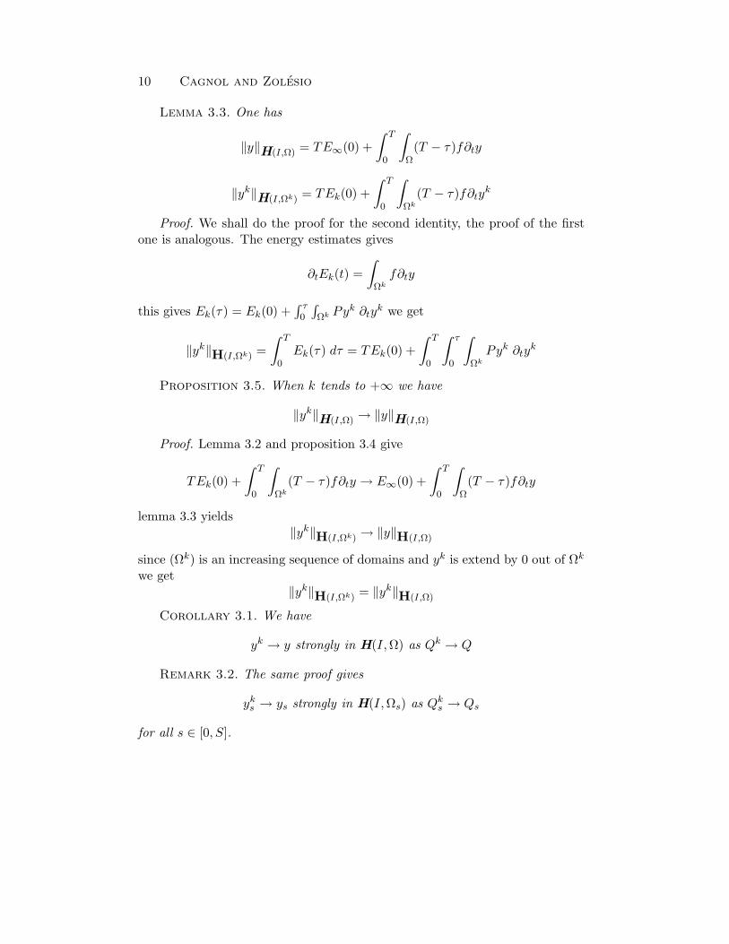
Lemma 3.3. One has
‖y‖H(I,Ω) = TE∞(0) +∫ T
0
∫Ω(T − τ)f∂ty
‖yk‖H(I,Ωk) = TEk(0) +∫ T
0
∫Ωk
(T − τ)f∂tyk
Proof. We shall do the proof for the second identity, the proof of the firstone is analogous. The energy estimates gives
∂tEk(t) =∫
Ωk
f∂ty
this gives Ek(τ) = Ek(0) +∫ τ0
∫Ωk Py
k ∂tyk we get
‖yk‖H(I,Ωk) =∫ T
0Ek(τ) dτ = TEk(0) +
∫ T
0
∫ τ
0
∫Ωk
Pyk ∂tyk
Proposition 3.5. When k tends to +∞ we have
‖yk‖H(I,Ω) → ‖y‖H(I,Ω)
Proof. Lemma 3.2 and proposition 3.4 give
TEk(0) +∫ T
0
∫Ωk
(T − τ)f∂ty → E∞(0) +∫ T
0
∫Ω(T − τ)f∂ty
lemma 3.3 yields‖yk‖H(I,Ωk) → ‖y‖H(I,Ω)
since (Ωk) is an increasing sequence of domains and yk is extend by 0 out of Ωk
we get‖yk‖H(I,Ωk) = ‖yk‖H(I,Ω)
Corollary 3.1. We have
yk → y strongly in H(I,Ω) as Qk → Q
Remark 3.2. The same proof gives
yks → ys strongly in H(I,Ωs) as Qks → Qs
for all s ∈ [0, S].

Sh. Sensitivity Analysis in Hyperbolic Pb. with non Smooth Domains 11
4 Shape Differentiability
4.1 Absolute Continuity
Let θ ∈ L1(I, L2(D)), we note
hk(s) =∫Qk
s
yksθ dx dt
h(s) =∫Qs
yθ dx dt
the shape differentiability for smooth domains gives
h′k(s) =∫Qk
s
y′sθ dx dt
Let y be the solution to the subsequent well-posed problemP (y) = 0 on Qy = − ∂y
∂n 〈V (0), n〉 on Σy(0) = 0 on Ω∂ty(0) = 0 on Ω
(12)
at this point we do not know that y is the shape derivative of the state functiony, and it is precisely what we are going to prove. Let us note
h(s) =∫Qs
ysθ dx dt
The absolute continuity of hk gives
∀k ∈ N∗, ∀s ∈ [0, S], hk(s) = hk(0) +
∫ s
0h′k(σ) dσ(13)
From proposition 3.4, the left hand side and the first term of the right handside converge to h(s) and h(0) respectively. To prove the absolute continuity ofh it is sufficient to prove that
∫ s0 h
′k(σ) dσ converges to∫ s0 h(σ) dσ as k tends
to +∞. To achieve that goal let us introduce the following adjoint problemP (Λks) = θ on QksΛks = 0 on Σk
s
Λks(T ) = 0 on Ωks
∂tΛks(T ) = 0 on Ωks
(14)
From proposition 3.1 we get
Λks → Λs strongly in H(I,Ωs) as Qks → Qs

12 Cagnol and Zolesio
Following [6] we haveLemma 4.1. Let Ks = (DTs)−1(K Ts)(∗DT−1
s ) then
h′k(s) =14
∫Σk
s
([∂(yks + Λks)
∂nks
]2
−[∂(yks − Λks)
∂nks
]2)⟨
Ksnks , n
ks
⟩⟨V (s), nks
⟩dΓ dt
For the sake of shortness we suppose K = I. Following [6] we haveLemma 4.2. Let µks ∈ L2(I,H1
0 (Ωks)) ∩ H1(I, L2(Ωk
s)) such that Pµks ∈L2(Qks) then ∫
Σks
(∂µks∂nks
)2 ⟨V (s), nks
⟩=
−2∫
Ωks
∂tµks(0)
⟨∇µks(0), V (s)(0)
⟩−∫Qk
s
⟨(div (V (s) − 2ε(V ))∇µks ,∇µks
⟩−2∫Qk
s
Pµks
⟨∇µks , V (s)
⟩+∫Qk
s
∂tµks2div (V − s) − 2∂tµks
⟨∇µks , V (s)
⟩Let µks,α = yks + αΛks with α ∈ −1; 1. It satisfies the hypothesis of lemma
4.2 since Pyks = f and PΛks = θ, Moreover yks and Λks as well as their timederivative and its gradient vanish on ΩsrΩk
s , therefore the integrals on Ωks and
Qks of lemma 4.2 can be replaced by integrals on Ωs and Qs respectively. Itfollows that hk(s) converges to∫
Σs
([∂(ys + Λs)
∂ns
]2
−[∂(ys − Λs)
∂ns
]2)〈Ksns, ns〉 〈V (s), ns〉 dΓ dt
it follows theProposition 4.1. One has
limk→+∞
hk(s) = h′(s)
From lemma 3.1, the real hk(s) is dominated by a constant independent ofs and k. Since aks and bks are bounded by a∗ and b∗ respectively.
Corollary 4.1. The function h is absolutely continuous.
4.2 Differentiability
Lemma 4.3. When s→ 0 one has
ys y in H1(I ×D)
Proof. Proposition 3.1 works with O = Ωs and µ = ys. Since we extend ysby zero out of Ωs we get
‖ys‖W 1,∞(I,L2(D))∩L∞(I,H1(D)) ≤ 2a∗ +√b∗

Sh. Sensitivity Analysis in Hyperbolic Pb. with non Smooth Domains 13
Since a∗ and b∗ depend only on the hold-all D, we extract a subsequenceconverging to an element y∗. The last point to be proven is that y∗ is solutionof (2). Even though we do not have an isotonic sequence, property 2.4 holdswhen replacing Ωk by Ωs and “k large enough” by “s small enough”. The onlyproblem is to prove y∗ vanishes on the lateral boundary Σ. Let dX denotethe distance to the set X. The convergence of the boundary gives dΩs → dΩ
strongly in L2(I ×D), hence
dΩsys → dΩy
in L2(I × D) as s → 0. Since ys = 0 on D r Ωs and dΩs = 0 on Ωs, we getdΩy = 0 hence y = 0 almost everywhere in DrΩ. As Ω is Lipschitz continuous,it has the Keldysh stability property, therefore y = 0 quasi everywhere in DrΩ.That yields y = 0 on ∂(D r Ω). We end up with y∗ = 0 on Σ.
Proposition 4.2. When s→ 0 one has
ys → y strongly in H1(I ×D)
Proof. The proof is based on the ideas of section 3.2. The energy to beconsidered is
12
∫Ωs
〈K∇ys(t),∇ys(t)〉 + (∂tys(t))2
Again, we do not have an isotonic sequence, however because Ωs is the imageof Ω by the flow mapping Ts, each compact of Ω is included in Ωs for s smallenough. We derive ‖ys‖H(I,Ωs)
→ ‖y‖H(I,Ω) when s → 0. That leads to‖ys‖H(I,D) → ‖y‖H(I,D).
Since a∗ and b∗ depend only on D, the domination of ‖ys‖H(I,D) isstraightforward. That proves
lims→0
h(s) = h(0)
That gives the weak shape differentiability in L1(I, L2(D)) of the state function.Remark 4.1. When m = 0, taking θ ∈ L∞(I, L2(Ω)) is required because
the weak shape differentiability for C2-boundary takes place in L1(I, L2(Ωk)).When m ≥ 1, the test θ can be taken L1(I, L2(θ)), that leads to the shapedifferentiability in L∞(I, L2(D)) of the state function.
References
[1] S. Agmon, Lectures on Elliptic Boundary Value Problems, Van Nostrand Mathe-matical Studies, 1965.

14 Cagnol and Zolesio
[2] C. Baiocchi and A. Capelo, Variational and quasivariational inequalities, JohnWiley & Sons Inc., New York, 1984.
[3] M. Berger and B. Gostiaux, Differential geometry: manifolds, curves, andsurfaces, Springer-Verlag, New York, 1988.
[4] D. Bucur, Controle par rapport au domaine dans les EDP, PhD thesis, Ecole desMines de Paris, 1995.
[5] J. Cagnol and J.-P. Zolesio, Hidden shape derivative in the wave equation, inSystems modelling and optimization (Detroit, MI, 1997), Chapman & Hall/CRC,Boca Raton, FL, 1999, pp. 42–52.
[6] , Shape derivative in the wave equation with Dirichlet boundary conditions,J. Differential Equations, 158 (1999), pp. 175–210.
[7] A. Chaira, Equation des ondes et regularite sur un ouvert lipschitzien, ComptesRendus de l’Academie des Sciences, Paris, series I, Partial Differential Equations,316 (1993), pp. 33–36.
[8] M. C. Delfour and J.-P. Zolesio, Structure of shape derivatives for non smoothdomains, Journal of Functional Analysis, 104 (1992), pp. 1–33.
[9] , Shape analysis via oriented distance functions, Journal of FunctionalAnalysis, 123 (1994), pp. 129–201.
[10] , Hidden boundary smoothness in hyperbolic tangential problems on non-smooth domains, in Systems modelling and optimization (Detroit, MI, 1997),Chapman & Hall/CRC, Boca Raton, FL, 1999, pp. 53–61.
[11] I. Lasiecka, J.-L. Lions, and R. Triggiani, Non homogeneous boundary valueproblems for second order hyperbolic operators, Journal de Mathematiques pureset Appliquees, 65 (1986), pp. 149–192.
[12] J. Necas, Sur les domaines de type N, Czechoslovak Math, 12 (1962), pp. 274–287.(Russian with a French summary).
[13] J.-P. Zolesio, Introduction to shape optimization and free boundary problems, inShape Optimization and Free Boundaries, M. C. Delfour, ed., vol. 380 of NATOASI, Series C: Mathematical and Physical Sciences, Kluwer Academic Publishers,1992, pp. 397–457.

Unbounded Growth of Total Variations of Snapshots
of the 1D Linear Wave Equation due to the ChaoticBehavior of Iterates of Composite Nonlinear
Boundary Reflection Relations
Goong Chen(1),(2), Texas A&M University, College Station, TexasTingwen Huang(1), Texas A&M University, College Station, TexasJonq Juang(3), National Chiao Tung University, Hsinchu, Taiwan, ROCDaowei Ma(4), Wichita State University, Wichita, Kansas
Abstract
Consider a linear one-dimensional wave equation on an interval. Ifthe boundary conditions are also linear, then the total variation of thegradient (wx(·, t), wt(·, t)) on the spatial interval remains bounded ast→ ∞, provided that the initial condition (w(·, 0), wt(·, 0)) has finite totalvariation. However, if we let the left-end boundary condition pump energyinto the system linearly, while the right-end boundary condition be self-regulating of the van der Pol type with a cubic nonlinearity, then chaoticvibrations occur when the parameters enter a certain regime. In this paper,we characterize the chaotic behavior of the gradient (wx(·, t), wt(·, t)) byproving that its total variation grows unbounded (with generically giveninitial conditions) as t→ ∞, even though the initial condition has a finitetotal variation. The proofs are obtained by the technique of intervalcovering sequences based on Stefan cycles and homoclinic orbits of thecomposite nonlinear boundary reflection map.
(1) E-mails: [email protected] and [email protected].
(2) Supported in part by Texas A&M University Interdisciplinary ResearchInitiative IRI 99-22.
(3) Work completed while on sabbatical at Texas A&M University. Supportedin part by a grant from NSC of R.O.C. E-mail: [email protected].
(4) E-mail: [email protected].
15

16 Chen et al.
1 Introduction
In this paper, we study a special property of chaotic vibration of thewave equation, that of unbounded growth of total variations of snapshots(wx(·, t), wt(·, t)) on the spatial interval of the one-dimensional (1D) waveequation as t→ ∞.
Earlier, in a series of papers [3–6], we have studied chaotic vibration of the1D wave equation
wxx(x, t) − wtt(x, t) = 0, 0 < x < 1, t > 0,(1.1)
subject to the following boundary conditions
left-end x = 0: wt(0, t) = −ηwx(0, t), η > 0, η 6= 1, t > 0;(1.2)
right-end x = 1: wx(1, t) = αwt(1, t) − βw3t (1, t), 0 < α ≤ 1, β > 0,
(1.3)
where the boundary condition (1.2) signifies energy injection or pumping intothe system, while (1.3) signifies a feedback with cubic nonlinearity of the vander Pol type. Note that in (1.1) we have set the spatial domain to be the unitinterval I ≡ (0, 1) just for convenience. Two initial conditions
w(x, 0) = w0(x), wt(x, 0) = w1(x), 0 < x < 1,(1.4)
are also prescribed. Then it was established in [5] that for fixed α, β, thecomposite reflection map Gη Fα,β : I → I is chaotic (cf. [5, (9)–(12)] or(1.9)–(1.10) below for Gη and Fα,β) and, therefore, for initial conditions (1.4)of generic type, (wx(x, t), wt(x, t)) displays chaotic behavior. Here, we followDevaney’s definition of chaos [8]; see also [2].
To make this paper sufficiently self-contained, let us repeat the solutionprocedure for (1.1)–(1.4) from [4] using the method of characteristics. Define
u(x, t) =12[wx(x, t) + wt(x, t)], v(x, t) =
12[wx(x, t) − wt(x, t)].(1.5)
Then (u, v) satisfies the following initial-boundary value problem (IBVP), afirst-order diagonalized symmetric hyperbolic system
∂
∂t
[u(x, t)v(x, t)
]=[
1 00 −1
]∂
∂x
[u(x, t)v(x, t)
], 0 < x < 1, t > 0,(1.6)
with boundary conditions
[u(0, t) − v(0, t)] = −η[u(0, t) + v(0, t)],(1.7)
u(1, t) + v(1, t) = α[u(1, t) − v(1, t)] + β[u(1, t) − v(1, t)]3.(1.8)

Unbounded Growth of Total Variations 17
The algebraic equations (1.7) and (1.8) define the reflection relations
v(0, t) = Gη(u(0, t)) ≡1 + η
1 − ηu(0, t),(1.9)
u(1, t) = Fα,β(v(1, t)),(1.10)
at, respectively, the left-end x = 0 and the right-end x = 1, where in (1.10),Fα,β : R → R is a nonlinear mapping such that for each given v ∈ R, u ≡ Fα,β(v)is the unique real solution of the cubic equation
β(u− v)3 + (1 − α)(u − v) + 2v = 0.(1.11)
The initial conditions are now
u(x, 0) = u0(x) = 12 [w′
0(x) + w1(x)],v(x, 0) = v0(x) = 1
2 [w′0(x) − w1(x)],
0 < x < 1.(1.12)
From time to time, we also need that u0 and v0 satisfy the compatibilityconditions
v0(0) = Gη(u0(0)), u0(1) = Fα,β(v0(1)).(1.13)
Using the maps Fα,β and Gη , we can represent the solution (u, v) of (1.6)explicitly as follows [5, (13), (14), p. 425]: for t = 2k + τ , k = 0, 1, 2, . . . ,0 ≤ τ < 2 and 0 ≤ x ≤ 1,
u(x, t) =
(Fα,β Gη)k(u0(x+ τ)), τ ≤ 1 − x,G−1η (Gη Fα,β)k+1(v0(2 − x− τ)), 1 − x < τ ≤ 2 − x,
(Fα,β Gη)k+1(u0(τ + x− 2)), 2 − x < τ < 2;
v(x, t) =
(Gη Fα,β)k(v0(x− τ)), τ ≤ x,Gη (Fα,β Gη)k(u0(τ − x)), x < τ ≤ 1 + x,(Gη Fα,β)k+1(v0(2 + x− τ)), 1 + x < τ < 2,
(1.14)
where (GηFα,β)n = (GηFα,β)(GηFα,β)· · ·(GηFα,β), the n-times iterativecomposition of Gη Fα,β. Since the solution representation (1.14) depend on(Gη Fα,β)n, it constitutes a natural Poincare section for the solution of (1.6).We say that the solution of (1.6) is chaotic if the map Gη Fα,β : I → I (orGη Fα,β : I → I, where I is an invariant subset of Gη Fα,β contained in I)is chaotic. Since (wx, wt) is topologically conjugate to (u, v) in the sense of [4,§5], we also say that the gradient w of the system (1.1)–(1.4) is chaotic.
The orbit diagram of the map Gη Fα,β, where α and β are held fixed, sayα = 1/2, β = 1, and only η is varying, can be seen from [5, Fig. 3, p. 433] (for0 < η < 1) and [5, Fig. 4, p. 434] (for η > 1), wherein period-doubling cascadesare manifest. For the purpose of making this paper sufficiently self-contained,

18 Chen et al.
we reproduce these two figures in Figs. 1 and 2, respectively. Furthermore, theexistence of homoclinic orbits has been established for the parameter range
(1 − 1 + α
3√
3
)/(1 +
1 + α
3√
3
)≤ η < 1, 1 < η ≤
(1 +
1 + α
3√
3
)/(1 − 1 + α
3√
3
).
(1.15)
See [5, Theorems 4.1 and 4.2, pp. 436–439].Let us now observe a few snapshots of the solution (u, v) of (1.6)–(1.12).
Choose initial conditions
w(x, 0) = 0.2 sin(π
2x), wt(x, 0) = 0.2 sin(πx), x ∈ [0, 1],(1.16)
and, thus
u0(x) = (0.1) ·[π2
cos(π
2x)
+ sin(πx)], v0(x) = (0.1) ·
[π2
cos(π
2x)− sinπx
](1.17)
are the initial conditions for (1.6)–(1.12). We display the snapshots of u(·, t)and v(·, t) using (1.14) in Figs. 3∼8, with the following parameter values:
α = 0.5, β = 1,(1.18)Figs. 3 ∼ 4 : η = 0.525, t = 52,(1.19)Figs. 5 ∼ 6 : η = 0.525, t = 102,(1.20)Figs. 7 ∼ 8 : η = 1.52 t = 52.(1.21)
For the value η = 0.525 used for Figs. 3–6, the map Gη Fα,β has just completedits period-doubling cascade, as can be seen from the orbit diagram [5, Fig. 3,loc. cit.]. Regarding the profiles of u and v, we see that as t increases fromt = 52 in (1.19) to t = 102 in (1.20), there is a very noticeable increase of“oscillatory ripples” from Figs. 3∼4 to Figs. 5∼6 (with the presence of some“macroscopically coherent periodic structure”). Let us further look at Figs. 7and 8, where for the parameter value η = 1.52 in (1.21), (1.15) implies theexistence of a homoclinic orbit (cf. (1.15)2); the profiles of u and v thereinlook extremely oscillatory at time t = 52, resembling something akin to “whitenoise”, along with the disappearance of any coherent patterns.
The highly oscillatory behavior of u and v as displayed in these figuresmotivated us to pose the following question:“[Q] Assume that the composite reflection map Gη Fα,β is chaotic. Doesthere exist a large class of initial conditions (u0, v0) for (1.6), (1.9), (1.10),and (1.12) such that VI(u0, v0) <∞ but
limt→∞
[VI((u(·, t)) + VI(v(·, t))] = ∞?”(1.22)
In (1.22), V[a,b](f) denotes the total variation of a given function f on interval[a, b]; see the definition in [1, p. 165], for example.

Unbounded Growth of Total Variations 19
Fig. 1. The orbit diagram of Gη Fα,βGη Fα,βGη Fα,β, with α = 0.5, β = 1α = 0.5, β = 1α = 0.5, β = 1, and ηηη being thevarying parameter, 0 < η < 10 < η < 10 < η < 1.
Fig. 2. The orbit diagram of Gη Fα,βGη Fα,βGη Fα,β, with α = 0.5, β = 1α = 0.5, β = 1α = 0.5, β = 1, and ηηη being thevarying parameter, η > 1η > 1η > 1.

20 Chen et al.
Fig. 3. The profile of u(x, t)u(x, t)u(x, t) at t = 52t = 52t = 52, with α = 0.5α = 0.5α = 0.5, β = 1, η = 0.525β = 1, η = 0.525β = 1, η = 0.525, for thesystem (1.6), (1.7), (1.8) and (1.17). (Reprinted from [5, p. 436], courtesy of WorldScientific, Singapore.)
Fig. 4. The profile of v(x, t)v(x, t)v(x, t) at t = 52t = 52t = 52, with α = 0.5, β = 1, η = 0.525α = 0.5, β = 1, η = 0.525α = 0.5, β = 1, η = 0.525, for thesystem (1.6) (1.7), (1.8) and (1.17). (Reprinted from [5, p. 346], courtesy of WorldScientific, Singapore.)

Unbounded Growth of Total Variations 21
Fig. 5. The profile of u(x, t)u(x, t)u(x, t) at t = 102t = 102t = 102, with α = 0.5, β = 1, η = 0.525α = 0.5, β = 1, η = 0.525α = 0.5, β = 1, η = 0.525, for thesystem (1.6) (1.7), (1.8) and (1.17). (Reprinted from [5, p. 437], courtesy of WorldScientific, Singapore.) The chaos here is due to the period-doubling cascade.
Fig. 6. The profile of v(x, t)v(x, t)v(x, t) at t = 102t = 102t = 102, with α = 0.5, β = 1, η = 0.525α = 0.5, β = 1, η = 0.525α = 0.5, β = 1, η = 0.525, for thesystem (1.6) (1.7), (1.8) and (1.17). (Reprinted from [5, p. 437], courtesy of WorldScientific, Singapore.) As with Fig. 5, the chaos here is due to the period-doublingcascade.

22 Chen et al.
Fig. 7. The profile of u(x, t)u(x, t)u(x, t) at t = 52t = 52t = 52, with α = 0.5, β = 1, η = 1.52α = 0.5, β = 1, η = 1.52α = 0.5, β = 1, η = 1.52, for thesystem (1.6) (1.7), (1.8) and (1.17). (Reprinted from [5, p. 442], courtesy of WorldScientific, Singapore.) The chaos here is due to a homoclinic orbit of Gη Fα,βGη Fα,βGη Fα,β.
Fig. 8. The profile of v(x, t)v(x, t)v(x, t) at t = 52t = 52t = 52, with α = 0.5, β = 1, η = 1.52α = 0.5, β = 1, η = 1.52α = 0.5, β = 1, η = 1.52, for thesystem (1.6) (1.7), (1.8) and (1.17). (Reprinted from [5, p. 442], courtesy of WorldScientific, Singapore.) As with Fig. 7, the chaos here is due to a homoclinic orbit ofGη Fα,βGη Fα,βGη Fα,β.

Unbounded Growth of Total Variations 23
In this paper, we give some informative answers to the question [Q] posedabove.
The rest of the paper is divided into three parts. In §2, we present a fewfacts about linear vibration in order to show the contrasts between linearity andnonlinearity. The main theorems are established in §3. In §4, miscellaneousdiscussions are given. A useful proposition, which was used in §2, is givenseparately in the Appendix near the end of the paper.
2 Bounds on the Total Variation of (u(·, t), v(·, t))(u(·, t), v(·, t))(u(·, t), v(·, t)) of the LinearWave Equation as t → ∞t → ∞t → ∞Consider the wave equation (1.1), but with linear boundary conditions such
as
left-end x = 0 : w(0, t) = 0, t > 0,(2.1)right-end x = 1 : wx(1, t) = 0, t > 0,(2.2)
in lieu of (1.2) and (1.3). Let the initial conditions satisfy
w(x, 0) = w0(x) ∈ H10 (0, 1), wt(x, 0) = w1(x) ∈ L2(0, 1),(2.3)
whereH1
0 (0, 1) = f : (0, 1) → R | f(0) = 0; f, f ′ ∈ L2(0, 1)is a Sobolev space with norm
‖f‖H10 (0,1) =
[∫ 1
0(f2 + f ′2)dx
]1/2
.
Then for the system (1.1), (2.1)–(2.3), the energy
E(t) =12
∫ 1
0[w2x(x, t) + w2
t (x, t)]dx(2.4)
is conserved and, therefore, we have the estimate
‖w(·, t)‖H10 (0,1) + ‖wt(·, t)‖L2(0,1) ≤ C(‖w0‖H1
0 (0,1) + ‖w1‖L2(0,1))(2.5)
for some constant C > 0 independent of (w0, w1). This type of Sobolevestimates is quite well known for the IBVP of the linear wave equation.
Not so well known are similar types of estimates in terms of total variationsfor the linear wave equation. Let us convert (1.1), and (2.1)–(2.3) into a first-order diagonalized symmetric hyperbolic system (1.6) through (1.5). Then (2.1)and (2.2) lead to the reflection relations
v(0, t) = G(u(0, t)) ≡ u(0, t), u(1, t) = F (v(1, t)) ≡ −v(1, t), t > 0.(2.6)

24 Chen et al.
Assume that the initial conditions u0 and v0 (cf. (1.12)) are continuous on Iand satisfy the compatibility conditions
v0(0) = G(u0(0)), u0(1) = F (v0(1)).(2.7)
Then from the representation formula (1.14) we easily obtain
VI(u(·, t)) + VI(v(·, t)) = VI(u0) + VI(v0), ∀ t > 0,(2.8)
i.e., the sum of the total variations of u and v at any t on I is conserved.If u0 and v0 are continuous on I but the compatibility conditions in (2.7) are
violated, then discontinuities can propagate along characteristics x − t = −k,x+ t = 1 + k for k = 0, 1, 2, . . . so (2.8) needs to be modified to
VI(u(·, t)) + VI(v(·, t)) ≤ VI(u0) + VI(v0) +C, ∀ t > 0,(2.9)
for some constant C:
C ≡ |u0(0) − v0(0)| + |u0(1) + v0(1)|.(2.10)
Using (1.5) and (2.9), we further deduce that
VI(wx(·, t)) + VI(wt(·, t)) ≤ 2[VI(w′0) + VI(w1) + C](2.11)
for some constant C > 0. From
w(x, t) =∫ x
0wx(ξ, t)dξ
and for any xk ∈ [0, 1] | k = 0, 1, . . . , n satisfying 0 = x0 < x1 < x2 < · · · <xn = 1,
n−1∑k=0
|w(xk+1, t) − w(xk, t)| =n−1∑k=0
∣∣∣∣∫ xk+1
xk
wx(ξ, t)dξ∣∣∣∣
≤n−1∑k=0
12
[∫ xk+1
xk
dξ +∫ xk+1
xk
w2x(ξ, t)dξ
]
=12
+∫ 1
0w2x(x, t)dx,(2.12)
we obtain
VI(w(·, t)) ≤ 12
+∫ 1
0w2x(x, t)dx.
Therefore (2.11) can be furthered strengthened. We summarize the above inthe following.

Unbounded Growth of Total Variations 25
Theorem 2.1. Consider the system (1.1), (2.1), (2.2) and (2.3), withw0 ∈ C1([0, 1]) and w1 ∈ C0([0, 1]). Then
VI(w(·, t)) + VI(wx(·, t)) + VI(wt(·, t)) ≤ 2[VI(w′0) + VI(w1) + E(0) + ˜
C],
(2.13)
for some ˜C > 0 depending only on C in (2.10).From the estimate (2.13) we see that if w0 ∈ C1(I) and w1 ∈ C0(I), then
as t → ∞, the left-hand side (LHS) of (2.13) remains bounded, provided thatinitially w′
0 and w1 have bounded total variations. The LHS of (2.13) can growunbounded (when and) only when initially (at least one of) w′
0 and w1 haveunbounded total variations. This is possible, as shown in the following example.
Example 2.1. Choose
w0(x) =∫ x
0ξ(ξ − 1) sin
1ξdξ, w1(x) = 0; 0 < x < 1.
Then (w0, w1) ∈ H10 (0, 1) × L2(0, 1). The compatibility conditions (2.7)1 and
(2.7)2 are satisfied. Therefore the solution (u, v) of (1.6), (2.6)–(1.12) iscontinuous for any (x, t) ∈ [0, 1] × [0,∞). Here
w′0(x) = x(x− 1) sin
1x, 0 < x < 1,
is easily verified to haveVI(w
′0) = ∞.
We see that the LHS of (2.13) is ∞ for any t > 0. Next, let us consider, again, linear boundary conditions but somewhat
different from the ones in (2.1) and (2.2). The IBVP system iswxx(x, t) − wtt(x, t) = 0, x ∈ (0, 1), t > 0,wt(0, t) + γw(0, t) = 0, t > 0,wx(1, t) = 0, t > 0,w(x, 0) = w0(x), wt(x, 0) = w1(x), x ∈ (0, 1).
(2.14)
Note that the boundary condition (2.14)2 is integrable along the t-direction:
w(0, t) = w(0, 0)e−γt, t ≥ 0.(2.15)
Again, converting (2.14) into a first-order diagonalized symmetric hyperbolicsystem using (1.5) and utilizing (2.15), we obtain the following snapshots att = 1, 2, . . . , inductively:
u0(x), v0(x) are given (according to (1.12)); and w(0, 0) is also known,u(x, k + 1) = −v(1 − x, k),v(x, k + 1) = u(1 − x, k) + γake
−γe−γ(1−x),ak+1 = w(0, k + 1) = e−γw(0, k), w(0, 0) ≡ a0.
(2.16)
26 Chen et al.
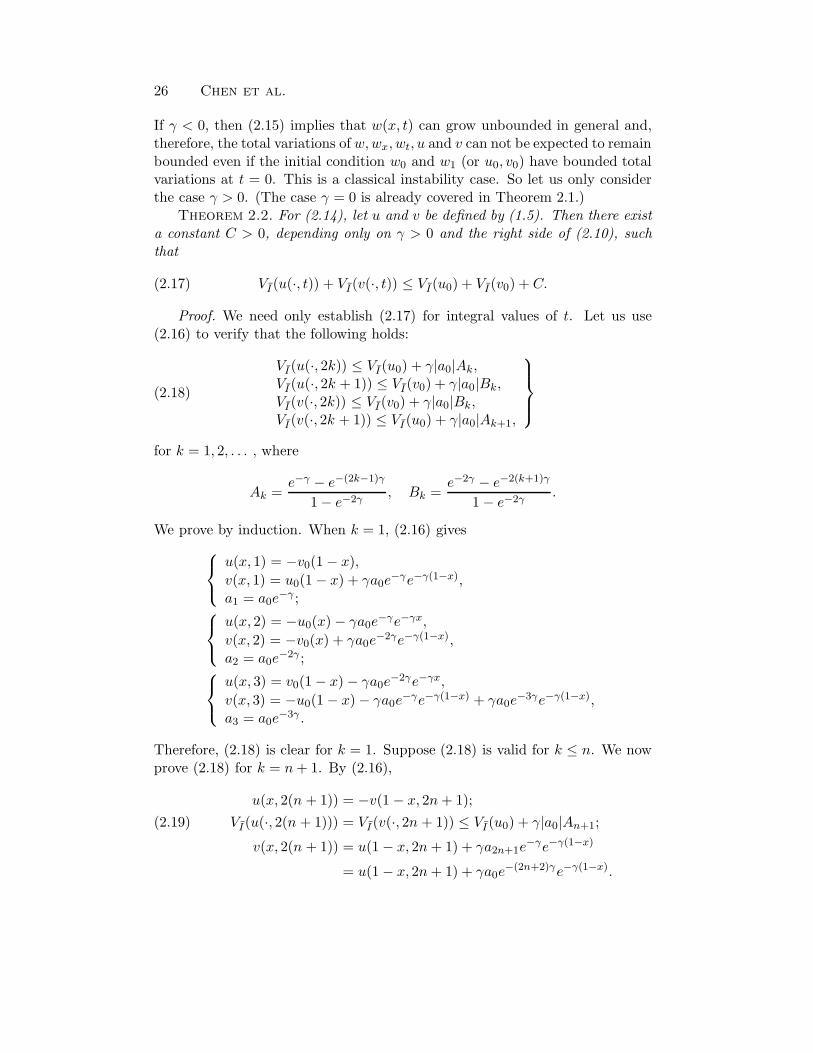
If γ < 0, then (2.15) implies that w(x, t) can grow unbounded in general and,therefore, the total variations of w,wx, wt, u and v can not be expected to remainbounded even if the initial condition w0 and w1 (or u0, v0) have bounded totalvariations at t = 0. This is a classical instability case. So let us only considerthe case γ > 0. (The case γ = 0 is already covered in Theorem 2.1.)
Theorem 2.2. For (2.14), let u and v be defined by (1.5). Then there exista constant C > 0, depending only on γ > 0 and the right side of (2.10), suchthat
VI(u(·, t)) + VI(v(·, t)) ≤ VI(u0) + VI(v0) + C.(2.17)
Proof. We need only establish (2.17) for integral values of t. Let us use(2.16) to verify that the following holds:
VI(u(·, 2k)) ≤ VI(u0) + γ|a0|Ak,VI(u(·, 2k + 1)) ≤ VI(v0) + γ|a0|Bk,VI(v(·, 2k)) ≤ VI(v0) + γ|a0|Bk,VI(v(·, 2k + 1)) ≤ VI(u0) + γ|a0|Ak+1,
(2.18)
for k = 1, 2, . . . , where
Ak =e−γ − e−(2k−1)γ
1 − e−2γ, Bk =
e−2γ − e−2(k+1)γ
1 − e−2γ.
We prove by induction. When k = 1, (2.16) givesu(x, 1) = −v0(1 − x),v(x, 1) = u0(1 − x) + γa0e
−γe−γ(1−x),a1 = a0e
−γ ;u(x, 2) = −u0(x) − γa0e
−γe−γx,v(x, 2) = −v0(x) + γa0e
−2γe−γ(1−x),a2 = a0e
−2γ ;u(x, 3) = v0(1 − x) − γa0e
−2γe−γx,v(x, 3) = −u0(1 − x) − γa0e
−γe−γ(1−x) + γa0e−3γe−γ(1−x),
a3 = a0e−3γ .
Therefore, (2.18) is clear for k = 1. Suppose (2.18) is valid for k ≤ n. We nowprove (2.18) for k = n+ 1. By (2.16),
u(x, 2(n + 1)) = −v(1 − x, 2n+ 1);VI(u(·, 2(n + 1))) = VI(v(·, 2n + 1)) ≤ VI(u0) + γ|a0|An+1;(2.19)
v(x, 2(n + 1)) = u(1 − x, 2n+ 1) + γa2n+1e−γe−γ(1−x)
= u(1 − x, 2n+ 1) + γa0e−(2n+2)γe−γ(1−x).

Unbounded Growth of Total Variations 27
Thus
VI(v(·, 2(n + 1))) ≤ VI(u(·, 2n + 1)) + VI(γa0e−2(n+1)γe−γ(1−x))
≤ VI(u(·, 2n + 1)) + γ|a0|e−2(n+1)γ
≤ VI(v0) + γ|a0|B2n + γ|a0|e−2(n+1)γ
= VI(v0) + γ|a0| ·[e−2γ − e−2(n+1)γ
1 − e−2γ+ e−2(n+1)γ
]
= VI(v0) + γ|a0| ·e−2γ − e−2(n+2)γ
1 − e−2γ
= VI(v0) +Bn+1.(2.20)
Therefore, (2.18)1 and (2.18)3 are verified by (2.19) and (2.20), respectively.The proof of (2.18)2 and (2.18)4 can be done in the same way. Therefore wehave proved (2.17).
Corollary 2.1. For the IBVP (2.14), assuming that w0 ∈ C1([0, 1]) andw1 ∈ C0([0, 1]). Then the estimate (2.13) holds for t > 0.
If, instead of the linear boundary conditions pair (2.14)2 and (2.14)3, weconsider
wx(0, t) − γw(0, t) = 0, γ > 0, t > 0,wt(1, t) = 0, t > 0,
(2.21)
where one of them is of Robin type [7, §1.2 and 1.3], then the treatmentbecomes much more challenging. After some extra efforts, we have succeededin establishing an estimate similar to (2.13), as shown below.
Theorem 2.3. Consider the system (1.1), (2.21), with initial conditionsw0 ∈ C1([0, 1]) and w1 ∈ C0([0, 1]) in (1.4). Then there exist two positiveconstants C1, C2 such that
VI(w(·, t)) + VI(wx(·, t)) + VI(wt(·, t)) ≤ C1[VI(w′0) + VI(w1)] + C2(2.22)
for all t > 0.Proof. First, we will establish the inequality
VI(u(·, t)) + VI(v(·, t)) ≤ C1[VI(u0) + VI(v0)] + C2(2.23)
for some positive constants C1 and C2, for all t > 0, from which (2.22) willnaturally follow. Here, as before, u, v, u0 and v0 are defined through (1.5) and(1.12).

28 Chen et al.
From (2.21)1, we have
[u(0, t) + v(0, t)] − γ
∫ t
0[u(0, τ) − v(0, τ)]dτ + w(0, 0)
= 0,
v(0, t) + γ
∫ t
0v(0, τ)dτ = −
[u(0, t) − γ
∫ t
0u(0, τ)dτ
]+ γw(0, 0),
e−γtd
dt
[eγt∫ t
0v(0, τ)dτ
]= −eγt d
dt
[e−γt
∫ t
0u(0, τ)dτ
]+ γw(0, 0),
which, after further simplification and integrations by parts, leads to
v(0, t) = −u(0, t) + 2γ∫ t
0e−γ(t−τ)u(0, τ)dτ + γw(0, 0)e−γt, t > 0.(2.24)
This is the reflection relation at the left end x = 0. At the right end x = 1, thereflection relation is
u(0, t) = v(0, t), t > 0.(2.25)
From (2.24) and (2.25), it is clear (based on a representation similar to (1.14))that (2.23) will hold if we can prove that there exist two positive constants C1
and C2 such that
V[0,T ](v(0, ·)) ≤ C1 · V[0,T ](u(0, ·)) + C1, for all T > 0,(2.26)
under the assumption of (2.24). (The reflection relation (2.25) is easy andsimple so it does not require any separate consideration.)
But (2.24) implies (2.26), following the application of a technical Proposi-tion A in the Appendix near the end of the paper.
We leave out the details that (2.23) yields (2.22).Note that if (2.21)2 is replaced by wx(1, t) = 0, then (2.25) correspondingly
will be changed tou(0, t) = −v(0, t)
and the arguments from (2.24) through (2.26) also need to be adaptedaccordingly. Nevertheless, such modifications are straightforward and theestimate (2.22) remains valid.
As a summary of this section, we have successfully shown that for majortypical homogeneous linear boundary conditions of the wave equation, the totalvariations of the snapshot of the gradient as well as the state of the waveequation at any time t on I will remain uniformly bounded in time, if theinitial total variation on I is finite.

Unbounded Growth of Total Variations 29
3 Unbounded Growth of the Total Variations of (u(·, t), v(·, t))(u(·, t), v(·, t))(u(·, t), v(·, t))as t → ∞t → ∞t → ∞ When Chaotic Vibration Occurs
This is the main section of the paper where we will treat question [Q].Let us first estimate the growth of total variations of (u(·, t), v(·, t)) due to
the post period-doubling of the reflection map Gη Fα,β.We will utilize special properties of the Stefan Cycle as given in Robinson
[11, pp. 67–70]. Let fµ : J → J be continuous on a finite closed interval J ⊂ R.Assume that fµ has completed a period-doubling cascade as the parameter µcrosses a value µ0. Therefore, we may now assume that fµ has a prime periodicpoint with period n = m ·2k, where m is an odd integer greater than or equal to3, as such an n is above the doubling cascade portion · · ·2j2j−1
2j−2· · ·2
in Sharkovskii’s ladder. From now on, to simplify notation, we just write fµ asf .
Define g = f2k. Then g has a periodic orbit
O = xj | j = 1, 2, . . . ,m(3.1)
of prime odd period m such that
g(xj) = xj+1, for j = 1, 2, . . . ,m− 1,(3.2)
satisfying either
xm < xm−2 < · · · < x3 < x1 < x2 < x4 < · · · < xm−1(3.3)
or
xm−1 < xm−3 < · · · < x4 < x2 < x1 < x3 < · · · < xm−2 < xm.(3.4)
Let us just treat the case (3.3) below because relation (3.4) is just a reflectionof (3.3) centered at x1 and all the arguments for (3.3) will also go through for(3.4) after a straightforward modification. Now define ([11, p. 67]) m−1 closedintervals
I1 = [x1, x2], I2 = [x3, x1], I3 = [x2, x4], . . . , I2j−1 = [x2j−2, x2j ],(3.5)I2j = [x2j+1, x2j−1], . . . , for j = 2, . . . , (m− 1)/2.
For two closed intervals J1 and J2, we say that J1 f -covers J2, in notationJ1
f−→ J2, if J2 ⊆ f(J1). Then we have the following.Proposition 3.1. ([11, p. 68]) Assume that J is a finite closed interval
and g : J → J is continuous with a prime periodic orbit of odd period m.Then there exist m− 1 closed subintervals I1, I2, . . . , Im−1 of J defined through(3.1)–(3.3) and (3.5) that overlap at most at endpoints such that
I1g−→ I2
g−→ I3g−→ · · · g−→ Im−1
g−→ I1g−→ I1 ∪ I2.(3.6)

30 Chen et al.
Theorem 3.1. Assume that J is a closed interval and g : J → J iscontinuous with a prime periodic orbit of odd period m. Then
limn→∞
VJ(gn) = ∞.(3.7)
Proof. We first show that
limk→∞
VI1(gkm) = ∞; see I1 defined in (3.5)).(3.8)
Utilizing (3.6), we have I1 gm-covers I1 ∪ I2. Therefore
VI1(gm) ≥ `(I1) + `(I2)
= (x2 − x1) + (x1 − x3) = x2 − x3, by (3.5),(3.9)
where `(Ij) denotes the length of the interval Ij . Also, since I1 gm-covers I1∪I2,we can find two subintervals I1,1 and I1,2 of I1, overlapping at most at endpoints,such that
gm(I1,1) = I1, gm(I1,2) = I2.(3.10)
Next, from (3.6) and (3.10), we have
I1,1gm
−→ I1g−→ I2
g−→ I3g−→ · · · Im−1
g−→ I1g−→ I1 ∪ I2,(3.11)
I1,2gm
−→ I2g−→ I3
g−→ I4g−→ · · · Im−1
g−→ I1g−→ I1
g−→ I1 ∪ I2,(3.12)
and, therefore, I1,1 has two subintervals I1,11 and I1,12 such that
g2m(I1,11) = I1 and g2m(I1,12) = I2,(3.13)
with I1,11 and I1,12 overlapping at most at endpoints. Similarly, from (3.12),we obtain two closed subintervals I1,21 and I1,22 of I1,2, overlapping at most atendpoints, such that
g2m(I1,21) = I1, g2m(I1,22) = I2.
We therefore obtain
VI1(g2m) ≥ VI1,11(g
2m) + VI1,12(g2m) + VI1,21(g
m) + VI1,22(gm)
≥ `(I1) + `(I2) + `(I1) + `(I2)= 2(x2 − x3).
This process can be continued indefinitely. In general, from a subintervalI1,a1a2...ak
where aj = 1 or 2 for j = 1, 2, . . . , k, we have
I1,a1a2...ak−1,1gkm
−→ I1g−→ I2
g−→ I3g−→ · · · g−→ Im−1
g−→ I1 ∪ I2,
I1,a1a2...ak−1,2gkm
−→ I2g−→ I3
g−→ I4g−→ · · · g−→ Im−1
g−→ I1g−→ I1 ∪ I2.

Unbounded Growth of Total Variations 31
From either of the above two sequences we can find two subintervals I1,a1...ak1
and I1,a1...ak2 of I1,a1...ak, overlapping at most at endpoints, such that
g(k+1)m(I1,a1...ak1) = I1 and g(k+1)m(I1,a1... ,ak2) = I2,
and because the collection of subintervals I1,a1a2...akak+1| aj = 1, 2; j =
1, 2, . . . , k + 1 has non-overlapping interior,
VI1(g(k+1)m) ≥
∑aj=1,2
j=1,... ,k+1
VI1,a1a2...akak+1(g(k+1)m))
≥ (k + 1)(x2 − x3) → ∞ as k → ∞.(3.14)
Therefore, we have established (3.8).To show (3.7), it is sufficient to show
limk→∞
VI1(gkm+j) = ∞, for j = 1, 2, . . . ,m− 1.
We utilize the covering sequence
I1gj
−→ Ij+1g−→ Ij+2
g−→ · · · g−→ Im−1g−→ I1
g−→ I1g−→ · · · g−→ I1︸ ︷︷ ︸
I1 appearingj+1 times
g−→ I1 ∪ I2
to deduce that I1 has two closed subintervals I(j)1,1 and I(j)
1,2 , overlapping at mostat endpoints, such that
gm+j(I(j)1,1) = I1, gm+j(I(j)
1,2) = I2.
Inductively, if I(j)1,a1... ,ak
is constructed, satisfying either
I(j)1,a1... ,ak−11
gkm+j
−−−−−−−→ I1g−→ I2
g−→ I3g−→ · · · g−→ Im−1
g−→ I1g−→ I1 ∪ I2,
or
I(j)1,a1...ak−12
gkm+j
−−−−−−−→ I2g−→ I3
g−→ I4g−→ · · · g−→ Im−1
g−→ I1g−→ I1
g−→ I1∪I2,
depending, respectively, on ak = 1 or 2, then we can find I(j)1,a1... ,ak
’s two
subintervals I(j)1,a1... ,ak1 and I
(j)1,a1... ,ak2, overlapping at most at endpoints, such
thatg(k+1)m+j(I(j)
1,a1...ak1) = I1, g(k+1)m+j(I(j)1,a1...ak2) = I2.
Again, we have
VI1(g(k+1)m+j) ≥
∑aj=1,2
j=1,... ,k+1
VI1,a1...ak+1(g(k+1)m+j) ≥ (k+1)(x2−x3) → ∞ as k → ∞.
The proof of (3.7) is now complete.

32 Chen et al.
Corollary 3.1. Assume that J is a closed interval f : J → J is continuouswith a prime periodic orbit of period m · 2k, where m is odd. Then
limn→∞
VJ(fn) = ∞.(3.15)
Proof. Let O1 = f `(ξ) | ` = 0, 1, . . . ,m ·2k−1 be an orbit of f with primeperiod m · 2k. Then O2 = f j·2k
(ξ) | j = 1, 2, . . . ,m is an orbit of g ≡ f2k
with prime period m. Write O2 in the form of (3.1) such that (3.2), (3.3) and(3.5) are satisfied. Therefore, we have O2 = xj | j = 1, 2, . . . ,m and for someinteger j1 : 0 < j1 ≤ m,
x1 = f j1·2k(ξ), x2 = f (j1+1)·2k
(ξ), . . . , xm = f (j1+m)·2k(ξ).
The main idea of the proof is to show that
limj→∞
VeI0(fj·(m·2k)+`) = ∞(3.16)
for any ` = 0, 1, 2, . . . ,m ·2k−1, for some subinterval I0 ⊆ J (where I0 dependson given `). Given any such ` ∈ 0, 1, 2, . . . ,m · 2k − 1, we can find a positiveinteger ˆ> 0 such that
`+ ˆ= j1 · 2k (modm · 2k).
Define
y1 = fˆ(ξ), y2 = f
ˆ+2k(ξ), I`0 =
[y1, y2], if y1 < y2,
[y2, y1], if y1 > y2.(3.17)
Then
f `(y1) = f `+ˆ(ξ) = f j1·2
k(ξ) = x1, f `(y2) = f `+
ˆ+2k(ξ) = f (j1+1)·2k
(ξ) = x2,
and we have the covering sequence
I`0f`
−→ I1g−→ I2
g−→ I3g−→ · · · g−→ Im−1
g−→ I1g−→ I1 ∪ I2,
where g = f2k. So I`0 contains two subintervals I`0,1 and I`0,2, overlapping at
most at endpoints, such that
fm·2k+`(I`0,1) = I1, fm·2k+`(I`0,2) = I2.
In general, if I`0,a1...apis constructed, for aj = 1, 2, j = 1, 2, . . . , p, satisfying the
following covering sequences

Unbounded Growth of Total Variations 33
(i) if ap = 1, then
I`0,a1... ,ap−11fpm·2k+`
−−−−−−−→ I1g−→ I2
g−→ · · · g−→ Im−1g−→ I1
g−→ I1 ∪ I2;
(3.18)
(ii) if ap = 2, then
I`0,a1...ap−12fpm·2k+`
−−−−−−−→ I2g−→ I3
g−→ · · · g−→ Im−1g−→ I1
g−→ I1g−→ I1 ∪ I2.
(3.19)
From (3.18) and (3.19), we have two subintervals I`0,a1...ap1 and I`0,a1...ap2 of
I0,a1...ap , such that
f (p+1)·m·2k+`(I`0,a1...ap1) = I1, f (p+1)·m·2k+`(I`0,a1...ap2) = I2.
The rest of the arguments follows in the same way as in the proof of Theorem 3.1.Therefore (3.16) follows from each ` ∈ 0, 1, . . . ,m·2k−1. Hence (3.15) follows.
Theorem 3.2. Consider the IBVP (1.6)–(1.8), and (1.12). Assumethat the composite reflection map f = Gη Fα,β has a periodic orbit O =f `(ξ) | ` = 0, 1, . . . ,m · 2k − 1, with prime period m · 2k, where m is odd.Further, assume that the initial conditions u0 and v0 in (1.12) are continuousand satisfy the compatibility conditions in (1.13) such that for some integerj0 : 0 ≤ j0 ≤ m · 2k − 1,
f j0(ξ), f j0+2k(ξ) ∈ Range z, z ≡ u0 or z ≡ v0.(3.20)
Then
limt→∞
[VI(u(·, t)) + VI(v(·, t))] = ∞.(3.21)
Proof. Let us assume that f j0(ξ), f j0+2k(ξ) ⊆ Range u0. Then we can
construct a subinterval I`0 as in (3.17) by letting ` = j0 therein. From the proofof Cor. 3.1 and (1.14), we easily deduce that
limn→∞
[VI(u(·, n)) + VI(v(·, n))] = ∞.
It is also easy to show that for any τ : 0 < τ < 1, by using the continuity ofthe total variations with respect to τ , that
limn→∞
[VI(u(·, n + τ)) + VI(v(·, n + τ))] = ∞.
Therefore (3.21) follows.

34 Chen et al.
Remark 3.1. It seems natural to believe that Theorem 3.2 remains valideven if condition (3.20) is weakened to the following:“there exist integers j1 and j2 : 0 ≤ j1 < j2 ≤ m · 2k − 1, such that
f j1(ξ), f j2(ξ) ∈ (Range u0) ∪ (Range v0).”(3.22)
However, in order to establish (3.21) under condition (3.22), the argumentsused in the proof of Cor. 3.1 also need to be considerably strengthened in orderto take care of the laborious “bookkeeping” details of finer interval coveringsequences, which we do not yet have an elegant way to handle so far.
Next, we study the growth of total variations of snapshots (u(·, t), v(·, t))when the composite reflection map Gη Fα,β has homoclinic orbits. There aretwo cases to be considered: (i) η > 1, and (ii) 0 < η < 1.
Write f = Gη Fα,β. Here we only consider the case that f has a boundedinvariant interval J such that f : J → J . For this to hold, we need [5,Lemma 2.5] either
(i) M ≡ 1 + η
1 − η
1 + α
3
√1 + α
3β≤ 1 + η
2η
√1 + αη
βη, if 0 < η < 1,(3.23)
or
(ii) M ≡ −1 + η
1 − η
1 + α
3
√1 + α
3β≤ 1 + η
2
√α+ η
β, if η > 1,(3.24)
in addition to (1.15), with
J = [−M,M ].(3.25)
Two graphs of f are provided in Figs. 9 and 10, where η = 0.552, 1.812,respectively.
Theorem 3.3. Assume that 0 < α ≤ 1, β > 0, η > 0 and η 6= 1. Assumealso that (1.15), (3.23)–(3.25) are also satisfied so that J = [−M,M ] is abounded invariant interval of Gη Fα,β. Then
limn→∞
VJ((Gη Fα,β)n) = ∞.
Proof. We first consider the case η > 1. Define a sequence of pointsxi ∈ J | i = 0, 1, 2, . . . as follows. Let
x0 = vI =√
1+αβ , the positive v-axis intercept of f [5, (32), p. 428],
x1 = minf−1(x0),x2 = f−1(x1),...xn+1 = f−1(xn),...
(3.26)

Unbounded Growth of Total Variations 35
Then for n = 0, 1, 2, . . . , xn ∈ J and xn ↓ 0 as n→ ∞. Also, define subintervals
I0 = [x1, x0], I1 = [x2, x1], . . . , In = [xn+1, xn], . . . .(3.27)
Then because f(I0) = [0, x1] we have the following covering sequence
Inf−→ In−1
f−→ In−2f−→ · · · f−→ I1
f−→ I0f−→
n⋃j=1
Ij(3.28)
f−→ Ikf−→ Ik−1
f−→ · · · f−→ I1f−→ I0
f−→n⋃`=1
I`, for k = 1, . . . , n.(3.29)
Therefore from (3.28), In has n subintervals In,j, j = 1, 2, . . . , n, overlappingat most at endpoints, such that
fn(In,j) = Ij , j = 1, 2, . . . , n.(3.30)
Fig. 9. A degenerate homoclinic orbit of the map f = Gη Fα,β, whereα = 0.5, β = 1α = 0.5, β = 1α = 0.5, β = 1 and η = 0.552η = 0.552η = 0.552. (Reprinted from [5, p. 426], courtesy of World Scientific,Singapore.)
Using the second part of the covering sequence in (3.29)
Ikf−→ Ik−1
f−→ · · · f−→ I0f−→ In−k
f−→ · · · f−→ I2f−→ I1
f−→ I0f−→
n⋃`=1
I`,

36 Chen et al.
Fig. 10. A degenerate homoclinic orbit of the map f = Gη Fα,βf = Gη Fα,βf = Gη Fα,β, whereα = 0.5α = 0.5α = 0.5, β = 1β = 1β = 1 and η = 1.812η = 1.812η = 1.812. (Reprinted from [5 p. 426], courtesy of World Scientific,Singapore.)
we also obtain n subintervals Ik,1, . . . , Ik,n of Ik, overlapping at most atendpoints, such that
fn(Ik,j) = Ij , j = 1, . . . , n; for k = 1, 2, . . . , n− 1.(3.31)
From (3.30) and (3.31), we obtain
V[0,x0](fn) ≥ V[xn+1,x0](f
n)
≥n∑
k,j=1
VIk,j(fn) ≥
n∑k=1
[(x0 − x1) + (x1 − x2) + · · · + (xn − xn+1)]
= n(x0 − xn+1) → ∞, as n→ ∞.(3.32)
Next, we consider the case 0 < η < 1. Let us modify (3.26) only slightly byredefining (3.26)2 as
x1 = maxf−1(x0), x1 < 0.(3.33)
The rest of (3.26) remains unchanged. Now, define intervals
I0 = [x2, x0], I1 = [x1, x3], I2 = [x4, x2], I3 = [x3, x5], . . . ,I2n = [x2n+2, x2n], I2n+1 = [x2n+1, x2n+3], . . . ,(3.34)
using the fact that
x1 < x3 < x5 < · · · < x2n+1 < · · · < 0 < · · · < x2n < x2n−2 < · · · < x4 < x2 < x0.

Unbounded Growth of Total Variations 37
Then because f(I0) = [x1, 0], we have the following covering sequence
I2n+1f−→ I2n
f−→ I2n−1f−→ · · · f−→ I1
f−→ I0f−→
n⋃j=0
I2j+1.
The rest of the proof can be done in the same way as in (3.28)–(3.32).Theorem 3.4. Consider the IBVP (1.6)–(1.8), (1.12). Assume that η
satisfies either (3.23) or (3.24) so that the composite reflection map f =Gη Fα,β has a bounded invariant interval J = [−M,M ] and a homoclinicorbit in J . Further, assume that the initial conditions u0 and v0 in (1.12)satisfy the compatibility conditions in (1.13) such that
Range z ⊇ In, z ≡ u0 or z ≡ v0 for some n ∈ 0, 1, 2, . . . , , cf. (3.27) or (3.34).(3.35)
Thenlimt→∞
[VI(u(·, t)) + VI(v(·, t))] = ∞.
Proof. Same as that of Theorem 3.2.Remark 3.2. We believe that (3.35) can be weakened at least to
Range u0∪ Range v0 ⊇ In, for some n ∈ 0, 1, 2, . . . .
Remark 3.3. The proof of Theorem 3.3 is essentially similar to those ofTheorem 3.1 and Corollary 3.1, and is based on the following fact:
“Let J be a finite closed interval and f : J → J is continuous.If f has a homoclinic orbit in J , then lim
n→∞VJ(fn) = ∞”.(3.36)
Actually, (3.36) above stands alone as a theorem itself and can also be provedby quoting the proofs of Theorem 3.1 and Corollary 3.1, provided that thehomoclinic orbit in (3.36) is nondegenerate, because by Theorem 1.16.5 inDevaney [8, p. 124], the map f is then topologically conjugate to the shift mapσ on
∑2 and, therefore, f has some periodic orbits of prime period m · 2k,
with m being odd and k ∈ 0, 1, 2, . . . . Hence the proofs of Theorem 3.1 andCorollary 3.1 apply.
When the homoclinic orbit in (3.36) is degenerate, then f is “more chaotic”(than the case when the homoclinic orbit is nondegenerate) and has homoclinicbifurcations. The renormalization procedure for the “model case” quadratic mapfµ(x) = µx(1−x) as µ→ 4 (the degenerate homoclinic orbit case) as mentionedin [8, §1.16] suggests that for µ = 4, f4 should be in the “post period doublingera” and therefore, f4 has many period-m · 2k orbits, with m being odd. It isquite obvious that our f in (3.36) ought to also have this kind of period-m · 2korbits (when the homoclinic orbit in (3.36) is degenerate) and, therefore, the

38 Chen et al.
proofs of Theorem 3.1 and Corollary 3.1 again apply. Nevertheless, we couldnot locate a precise reference to this effect.
In passing, we may also note that the condition (3.35) is stated quitedifferently from (3.20), in the sense that the end-points of intervals In in (3.35)are not periodic points. (Or rather, the end-points of In have an “infiniteperiodicity”.)
4 Miscellaneous Remarks
In this paper, we have successfully shown that when chaotic vibration occursfor the wave equation caused by the nonlinear boundary condition specifiedhere, the total variations of snapshots tend to infinity as t → ∞ for a largeclass of initial data, even though the total variation of any such initial datais finite at time t = 0. Our theorems in §3 have covered the case of “stable”chaos on a bounded invariant interval. A different type of “unstable” chaos,discussed in [5, §5], happens on an invariant Cantor set (rather than a boundedinvariant interval, because the map Gη Fα,β does not have one for that set ofα, β and η values). In that case, it is trivial to show that the total variations ofsnapshots also tend to infinity as t → ∞ for a large class of initial data, eventhough initially, the total variation of the state is finite.
One may ask a converse question to [Q]:“[−Q] Assume that there exist initial conditions (u0, v0) for (1.6), (1.9), (1.10)and (1.12) and an invariant interval I of Gη Fα,β such that
VI(u0, v0) <∞, VI(u(·, t)) + VI(v(·, t)) → ∞ as t → ∞.(4.1)
Is the map Gη Fα,β necessarily chaotic?”The answer is negative, as the following counterexample has shown.Example 4.1. Let α = 0.5, β = 1, either η ∈ (0, 0.433) or η ∈ (2.312,∞).
Then as Figs. 1 and 2 ([5, Figs. 3 and 4, pp. 433–434]) have shown, the mapGη Fα,β has a locally attracting period-2 orbit near 0, which is repelling.
Let g(x) = x2. For x ∈ [0, 1],
u0(x) =
x2, if x =1n, n = 1, 2, . . . ,
0, if x =2n + 1
2n(n+ 1), n = 1, 2, . . . ,
2(n+ 1)n
x− 2n+ 1n2
, if x ∈[ 2n+ 12n(n + 1)
,1n
]− 2nn+ 1
x+2n+ 1
(n+ 1)2, if x ∈
[ 1n+ 1
,2n+ 1
2n(n+ 1)
).
(4.2)
Then u0(x) is continuous. Choose any v0, continuous of bounded total variationsatisfying the compatibility condition (1.13). On each subinterval
[1
n+1 ,1n
], the

Unbounded Growth of Total Variations 39
total variation of u0 is 1/n2 + 1/(n + 1)2. Therefore u0 has bounded totalvariation on the interval [0,1]. Let the period-2 orbit of Gη Fα,β be p,−p,where p > 0. Then for each y ∈ [0, 1], y 6= 1
n for n = 1, 2, . . . , we have
limn→∞
|(Gη Fα,β)n(u0(y))| = p.
Therefore, on each subinterval[
1n+1 ,
1n
], the total variation of (GηFα,β)n tends
to p, and
limt→∞
[VI(u(·, t)) + VI(v(·, t))] = ∞, but VI(u0) + VI(v0) <∞.(4.3)
The above negative result seems to have weakened the connection between
chaotic vibration and unbounded growth of total variations of snapshots.However, we may take note of the following recent result in [10]. Let
f : J → J be chaotic (according to Devaney [8, p. 50]), on the finite closedinterval J . Then f has sensitive dependence on initial data [2]. This sensitivedependence on initial data is regarded as a major feature of chaotic maps; [10]has proved the following:
“(i) Let f : J → J has sensitive dependence on initial data. Thenlimn→∞
VJ ′(fn) = ∞ for every closed subinterval J ′ of J .
(ii) Let f : J → J be continuous with finitely many extremal points,satisfying lim
n→∞VJ ′(fn) = ∞ for every closed subinterval J ′ of J . Then f
has sensitive dependence on initial data.”
The theorems in [10] actually explains why the breakdown (4.3) happens: theinitial data in (4.2) has infinitely many extremal points, i.e., there are infinitelymany oscillations on a finite closed interval and, thus, it is “too oscillatory”.
The growth rate of VI(fn) as estimated in (3.14) and (3.32) are linear with
respect to n. Sharper estimates may also be possible, at least for certain specialcases. In [9], examples of exponential growth have been found. Related issuessuch as Remarks 3.1 and 3.2 and others are also being investigated in [9].
Appendix A Key Proposition
In this section, we prove the following.
Proposition A. Assume that u and v are related through
v(t) = αu(t) + β
∫ t
0e−γ(t−τ)u(τ)dτ + f(t), t ≥ 0,(A.1)

40 Chen et al.
where α, β ∈ R, γ > 0. Then
V[0,T ](v) ≤(|α| + |β|
γ
)V[0,T ](u) +
|β|γ|u(0+)| + V[0,T ](f),(A.2)
for all T > 0, where u(0+) = limt→0+
u(t).
We first establish the following technical lemma.
Lemma B. Let γ > 0 and
g(t) = [Qu](t) ≡∫ t
0e−γ(t−τ)u(τ)dτ, ∀ t ≥ 0.
Then
V[0,T ](g) ≤1γ
[|u(0+)| + V[0,T ](u)], ∀ T > 0.(A.3)
Proof.
(1) We first assume that u is increasing and continuous. Then
g′(t) = −γ∫ t
0e−γ(t−s)u(s)ds + u(t)
= −e−γ(t−s)u(s)∣∣∣s=ts=0
+∫ t
0e−γ(t−s)du(s) + u(t)
= e−γtu(0) +∫ t
0e−γ(t−s)du(s).(A.4)
Note that the integral in (A.4) is a Stieltjes integral [1, Chap 9]. Since gis absolutely continuous, we see that
V[0,T ](g) =∫ T
0|g′(t)|dt ≤ |u(0)|
∫ T
0e−γtdt+
∫ T
0
∫ t
0e−γ(t−s)du(s)dt
≤ 1γ|u(0)| +
∫ T
0
(∫ T
se−γtdt
)eγsdu(s)
=1γ|u(0)| + 1
γ
∫ T
0(e−γs − e−γT )eγsdu(s)
≤ 1γ|u(0)| + 1
γ
∫ T
0du(s)
=1γ|u(0) +
1γ
[u(T ) − u(0)]
=1γ
[|u(0)| + V[0,T ](u)].
Therefore (A.3) is true when u is increasing and continuous.

Unbounded Growth of Total Variations 41
(2) We now assume that u is increasing and left-continuous. Then
u = u0 +∑c∈J
rcHc,(A.5)
where u0 is increasing and continuous, u0(0) = u(0+), J is a (possiblyempty) countable set of nonnegative real numbers, rc > 0, and
Hc(t) =
0, 0 ≤ t ≤ c,1, t > c,
is the Heaviside function. Then
V[0,T ](u) = V[0,T ](u0) +∑
c∈J,c<Trc,
hc(t) ≡ [QHc](t) =∫ t
0e−γ(t−s)Hc(s)ds =
0, 0 ≤ t ≤ c,1γ
[1 − e−γ(t−c)], c < t.
Since hc(t) is increasing, V[0,t](hc) = hc(T ) and, thus,
V[0,T ](hc)
= 0, if T ≤ c,
≤ 1γ, for all T ≥ 0.
From (A.5), g = Qu0 + ΣrcQHc, so
V[0,T ](g) ≤ V[0,T ](Qu0) +∑
rcV[0,T ](QHc)
≤ 1γ
[|u0(0)| + V[0,T ](u0)] +∑c<T
rcγ
(by part (1))
=1γ
[|u(0+)| + V[0,T ](u)].
Therefore (A.2) is proved for increasing, left-continuous function u.
(3) Now we consider a left-continuous function u. Define
u1(t) =12[V[0,t](u) + u(t) + u(0)],
u2(t) =12[V[0,t](u) − u(t) + u(0)].
Then u1 and u2 are both left-continuous, increasing functions, and u =u1 − u2, V[0,T ](u) = V[0,T ](u1) + V[0,T ](u2), u1(0+) = u(0+), u2(0+) = 0.

42 Chen et al.
By part (2) above,
V[0,T ](g) ≤ V[0,T ](Qu1) + V[0,T ](Qu2)
≤ 1γ
[|u1(0+)| + V[0,T ](u1)] +1γ
[|u2(0+)| + V[0,T ](u2)]
=1γ|u(0+)| + 1
γV[0,T ](u).
(4) We can now consider the general case. Let
u(t) =
lims→t−
u(s), for t > 0,
u(0), if t = 0.
Then u is left-continuous, Qu = Qu, V[0,T ](u) ≤ V[0,T ](u) and u(0+) =u(0+). By part (3),
V[0,T ](g) = V[0,T ](Qu) = V[0,T ](Qu)
≤ 1γ
[|u(0+)| + V[0,T ](u)] ≤1γ
[|u(0+)| + V[0,T ](u)].
Therefore (A.3) is proved.
Proof. [Proof of Proposition A] From (A.1), we have, by (A.3),
V[0,T ](v) ≤ |α|V[0,T ](u) + |β| · 1γ
[|u(0+)| + V[0,T ](u)] + V[0,T ](f).
Therefore, (A.2) holds.
References
[1] T.M. Apostal, Mathematical Analysis, Addison Wesley, Reading, MA, 1957.[2] J. Banks, J. Brooks, G. Cairns, G. Davis and P. Stacey, On Devaney’s definition
of chaos, Amer. Math. Monthly 99 (1992), 332–334.[3] G. Chen, S.B. Hsu and J. Zhou, Linear superposition of chaotic and orderly
vibrations on two serially connected strings with a van der Pol joint, Int. J.Bifurcation and Chaos 6 (1996), 1509–1527.
[4] G. Chen, S.B. Hsu and J. Zhou, Chaotic vibrations of the one-dimensionalwave equation due to a self-excitation boundary condition, Part I: Controlledhysteresis, Trans. Amer. Math. Soc. 350 (1998), 4265–4311.
[5] G. Chen, S.B. Hsu and J. Zhou, Chaotic vibration of the one-dimensional waveequation due to a self-excitation boundary condition, Part II: Energy injection,period doubling and homoclinic orbits, Int. J. Bifurcation and Chaos 8(3) (1998),423–445.

Unbounded Growth of Total Variations 43
[6] G. Chen, S.B. Hsu and J. Zhou, Chaotic vibrations of the one-dimensional waveequation due to a self-excitation boundary condition, Part III: Natural hysteresismemory effect, Int. J. Bifurcation and Chaos 8(3) (1998), 447–470.
[7] G. Chen and J. Zhou, Vibration and Damping in Distributed Systems, Vol I:Analysis, Estimation, Attenuation and Design, CRC Press, Boca Raton, FL, 1993.
[8] R.L. Devaney, An Introduction to Chaotic Dynamical Systems, Addison-Wesley,New York, 1989.
[9] T.W. Huang, Ph.D. Dissertation, Department of Mathematics, Texas A&MUniversity, in progress.
[10] T.W. Huang and G. Chen, Chaotic behavior of interval maps as characterized byunbounded growth of total variations of their n-th iterates as n→ ∞, preprint.
[11] C. Robinson, Dynamical Systems, Stability, Symbolic Dynamics and Chaos, CRCPress, Boca Raton, FL, 1995.

44 Chen et al.

Velocity method and Courant metric topologies in
shape analysis of partial differential equations
Michel C. Delfour1, Universite de Montreal, C. P. 6128, Montreal Qc, CanadaH3C 3J7, E-mail: [email protected] Zolesio, CNRS, Centre de Mathematiques Appliquees, Ecole desMines, INRIA, 2004 route des Lucioles, BP 93, 06902 Sophia Antipolis Cedex,France. E-mail: [email protected]
AbstractThe object of this paper is to give the equivalence between the
continuity of a shape function with respect to the generic complete Courantmetric topology introduced by A.M. Micheletti in 1972 and its continuityalong the flow of non-autonomous velocity fields. This result also clarifiesthe connection between spaces of domains endowed with a Courant metricand the Velocity Method used in the definition of semiderivatives of shapefunctions.
1 Introduction
The Shape Analysis of partial differential equations deals with problems wherethe underlying domain has a free boundary, changes with time, or is a controlor design variable. Spaces of shapes or geometries are usually nonlinear andnonconvex spaces. The dependence of the solution of a pde with respect tothe domain as a variable is also nonlinear. Perhaps the first appearance of thegeometry as a time-dependent variable in Control Theory is due to Bardos andChen [1] who showed that stabilization of the wave equation could be achievedby moving (time like) the boundary of the domain. Truchi and Zolesio [8]extended this result to membrane equations by periodic motion of the boundary.More recently D.L. Russell introduced the notion of formability [7]2 which canbe seen as an equivalent of controllability for shapes. There are many waysto tackle this general class of problems. For instance the Velocity Method was
1This paper was completed while the first author was on sabbatical leave at INRIA-Rocquencourt (France) in the projects MACS and SOSSO. The research of the first author hasbeen supported by National Sciences and Engineering Research Council of Canada researchgrant A–8730 and by a FCAR grant from the Ministere de l’Education du Quebec.
2The ”theory of formability” characterizes the ability to deform a body into a prescribedshape through control of the microstructure of the material.
45

46 M.C. Delfour and Jean-Paul Zolesio
used by Truchi and Zolesio while the Courant metric was used by Micheletti [5]to study the dependence of the first eigenvalue of an elliptic pde with respectto the domain.
The admissible domains are often defined as the set of images of a fixedsubset of RN through a family of transformations of RN. The compositionof transformations induces a natural group structure on images and the fullpower of function analytic methods is available to define a topology on thegroup. The choice is obviously very much problem dependent. In 1972 A.M.Micheletti [5] gave perhaps one of the first complete metric topologies on afamily of domains of class Ck which are the images of a fixed bounded openconnected domain of class Ck through a family of Ck diffeomorphisms of RN.Her analysis culminates with the construction of the Courant metric whichmakes the associated quotient group of diffeomorphisms a complete metricspace. Her construction and results are quite general and even generic forother families of transformations of RN including the ones considered by Muratand Simon [6] later in 1976.
Another point of view is the so called Velocity Method (cf. [10, 9, 3, 4]),where the transformations of RN which define the variations of the shape areconstructed from the flow of non-autonomous velocity fields. This has beenextensively used to define semiderivatives of a shape function with respect tothe shape of the underlying domain.
This paper deals with the long standing issue of the connection between theVelocity Method and topologies generated by Courant metrics. Its main objectis to give the equivalence between the continuity of a shape function with respectto the generic complete Courant metric topology and its continuity along theflow of non-autonomous velocity fields. We specialize the equivalence for thetransformations associated with the spaces Ck+1
0 (RN,RN), Ck+1(RN,RN), andCk,1(RN,RN)3.
2 Courant metric topology on Ck domains
In this section we recall and quote the main constructions and results in [5].
Given an integer k ≥ 1, denote by Ck(RN)def= Ck(RN,RN) the space of k-times
continuously differentiable transformations f of RN. When endowed with thenorm
‖f‖Ckdef= max
0≤|α|≤k‖∂αf‖C , ‖∂αf‖C
def= sup
x∈RN
|∂αf |,
3For k ≥ 0, Ck+10 (RN,RN) is the space of all (k + 1)-times continuously differentiable
mappings f : RN → RN for which f and all its partial derivatives up to order k + 1 vanishat infinity. Ck+1(RN,RN) is the space of mappings f : RN → RN for which f and ∂αf arebounded and uniformly continuous on RN for all α, 1 ≤ |α| ≤ k + 1. Ck,1(RN,RN) is thespace of mappings f : RN → RN for which f and ∂αf are bounded and uniformly Lipschitzcontinuous on RN for all α, 1 ≤ |α| ≤ k.

Velocity method and Courant metric topologies 47
Ck0 (RN)def= Ck0 (RN,RN) is a Banach space. Associate with Ck0 (RN) the space
Fk0
def=F : RN → RN : F − I ∈ Ck0 (RN) and F−1 ∈ Ck(RN)
.
Theorem 2.1. For k ≥ 1 the space Fk0 is a group with respect to the composition
of transformations.Lemma 2.1. Given f and g in Ck(RN), let ψ = f (I + g). Then for eachx ∈ RN
|ψ(x)| = |f(x+ g(x))||ψ(1)(x)| ≤ |f (1)(x+ g(x))| [1 + |g(1)(x)|]
|ψ(i)(x)| ≤ |f (1)(x+ g(x))| |g(i)(x)|
+i∑
j=2
|f (j)(x+ g(x))| aj(|g(1)(x)|, . . . , |g(i−1)(x)|)
for i = 2, . . . , k where aj is a polynomial.Lemma 2.2. Given integers r ≥ 0 and s > 0 there exists a constant c(r, s) > 0with the following property: if the sequence f1, . . . , fn in Cr(RN) is such that
n∑i=1
‖fi‖Cr < α, 0 < α < s,(2.1)
then for the map F = (I + fn) · · · (I + f1)
‖F − I‖Cr ≤ α c(r, s).(2.2)
Associate with a fixed open or closed subset4 Ω0 of RN the following familyof images of Ω0 by the elements of Fk
0
X (Ω0)def=F (Ω0) ⊂ RN : ∀F ∈ Fk
0
This induces a bijection
[F ] 7→ F (Ω0) : Fk0 /G(Ω0) → X (Ω0).(2.3)
between X (Ω0) and the quotient group of Fk0 by the subgroup
G(Ω0)def=F ∈ Fk
0 : F (Ω0) = Ω0
(2.4)
4In her paper [5] A.M. Micheletti assumes that Ω0 is a bounded connected open domainof class Ck in order to make all the images F (Ω0) bounded connected open domains of classCk. However the construction of the Courant metric only requires that Ω0 be closed or open.

48 M.C. Delfour and Jean-Paul Zolesio
of transformations which map Ω0 onto Ω0.The next step is to construct a complete metric space topology on Fk
0 whichinduces a complete metric space topology on the quotient group Fk
0 /G(Ω0). Thespace X (Ω0) is then identified with the topological quotient group Fk
0 /G(Ω0).This quotient metric is called the Courant metric by A.M. Micheletti. Theconstruction of the metric topology on Fk
0 /G(Ω0) is not as straightforward asit might appear at first sight. The obvious candidates for the metric do notusually satisfy the triangle inequality and only yield a pseudo-metric on thequotient group. In order to get around this difficulty Micheletti introduced thefollowing construction. Given F ∈ Fk
0 , consider finite factorizations of F andF−1 of the form
F = (I + fn) · · · (I + f1) and F−1 = (I + gm) · · · (I + g1)
Define
d(I, F )def= inf
(f1,...,fn)
n∑i=1
‖fi‖Ck + inf(g1,...,gm)
m∑i=1
‖gi‖Ck(2.5)
where the infima are taken with respect to all finite factorizations of F and F−1
in Fk0 . Extend this definition to all pairs F and G in Fk
0
d(F,G)def= d(I,G F−1)(2.6)
By definition d is right-invariant since for all F , G and H in Fk0
d(F,G) = d(F H,G H)(2.7)
and the three axioms which define a metric on Fk0 are verified.
Theorem 2.2. Fk0 is a complete metric group.
Corollary 2.1. The topology induced by the metric d on the topological groupFk
0 coincides with the topology which has as a basis of neighborhoods of theidentity in Fk
0 the sets
E(ε) def=F ∈ Fk
0 : ‖F − I‖Ck + ‖F−1 − I‖Ck < ε.
It is readily seen that we have the following properties.Lemma 2.3. Given an open or a closed5 subset Ω0 of RN, the family
G(Ω0)def=F ∈ Fk
0 : F (Ω0) = Ω0
is a closed subgroup of Fk
0 .
5As noted earlier it is not necessary that Ω0 be a bounded connected open Ck domain.

Velocity method and Courant metric topologies 49
By definition for each Ω ∈ X (Ω0) there exists F ∈ Fk0 such that Ω = F (Ω0).
Therefore the following map is well-defined and bijective
Ω 7→ χ(Ω) = F G(Ω0) : X (Ω0) → Fk0 /G(Ω0).(2.8)
Using χ we now introduce the following complete metric on X (Ω0).Theorem 2.3. Given an open or a closed subset Ω0 of RN, the function
δ(F G(Ω0),H G(Ω0))def= inf
G,G∈G(Ω0)d(F G,H G)(2.9)
is a metric on Fk0 /G(Ω0). The topology induced by δ coincides with the quotient
topology of Fk0 /G(Ω0) and the space Fk
0 /G(Ω0) is complete.Finally it is natural to define on X (Ω0) the following metric
ρ(Ω1,Ω2)def= δ(χ(Ω1), χ(Ω2))(2.10)
induced by the bijection χ on X (Ω0). With that metric, X (Ω0) is a completemetric space. This metric is called the Courant metric (metrica di Courant) in[5].
3 The generic framework of Micheletti
The construction of a complete metric topology on the group and a Courantmetric on the quotient group naturally extends to other underlying spaces Θthan the Banach space Ck0 (RN). Given a Banach space Θ of transformations ofRN, define the space
F(Θ)def=F : RN → RN : F − I ∈ Θ and F−1 − I ∈ Θ
.
Associate with F ∈ F(Θ) the distance
d(I, F )def= inf
(f1,...,fn)
n∑i=1
‖fi‖Θ + inf(g1,...,gm)
m∑i=1
‖gi‖Θ,(3.1)
where the infima are taken over all finite factorizations in F(Θ) of the form
F = (I + fn) · · · (I + f1) and F−1 = (I + gm) · · · (I + g1), fi, gi ∈ Θ.
Extend this definition to all pairs F and G in F(Θ)
d(F,G)def= d(I,G F−1)(3.2)

50 M.C. Delfour and Jean-Paul Zolesio
Define for some fixed open or closed subset Ω0 of RN the subgroup
G(Ω0)def= F ∈ F(Θ) : F (Ω0) = Ω0
and the Courant metric on the equivalence classes of F(Θ)/G(Ω0)
∀F, G ∈ F(Θ), δ([F ], [H)]def= inf
G,G∈G(Ω0)d(F G,H G)(3.3)
∀F1, F2 ∈ F(Θ), ρ(F1(Ω0), F2(Ω0))def= δ([F1], [F2])(3.4)
on the images F (Ω0) of Ω0 by elements F of F(Θ). Of course F(Θ)/G(Ω0)will be a well-defined complete metric space for the Courant metric only forappropriate choices of spaces Θ.
As an illustration consider the spaces of transformations of RN introducedby Murat and Simon [6] in 1976 in the construction of metric spaces of domains.For integers k ≥ 0, they correspond to the following choices of the space Θ:
W k+1,c(RN,RN)def=
f ∈W k+1,∞(RN,RN) : ∀ 0 ≤ |α| ≤ k + 1, ∂αf ∈ C(RN,RN)
and W k+1,∞(RN,RN). The first space W k+1,c(RN,RN) algebraically and
topologically coincides with the space Ck+1(RN)def= Ck+1(RN,RN). The
corresponding space of transformations
Fk+1(RN)def=F : RN → RN :F − I ∈ Ck+1(RN) and F−1 − I ∈ Ck+1(RN)
is a topological group for the metric d as in the case of Fk+1
0 in § 2. The
second space W k+1,∞(RN,RN) coincides with Ck,1(RN)def= Ck,1(RN,RN). The
associated space of transformations
Fk,1(RN)def=F : RN → RN :F − I ∈ Ck,1(RN) and F−1 − I ∈ Ck,1(RN)
(3.5)
is complete for the topology induced by the metric d, but is not a topologicalgroup. In both cases the Courant metric defines a complete metric topology onthe corresponding quotient space. Also recall from [6] that F1(RN) transportslocally Lipschitzian (graph) domains onto locally Lipschitzian (graph) domainsbut that F0,1(RN) does not.

Velocity method and Courant metric topologies 51
3.1 Approach of Murat and Simon
The construction introduced by Murat and Simon [6] to obtain a completemetric topology on the quotient spaces are different from the ones of Micheletti[5] which were seemingly not known to them. They worked with the pseudo-metric
dp(F2, F1)def= ‖F2 F−1
1 − I‖W k+1,∞ + ‖F1 F−12 − I‖W k+1,∞
rather than the metric defined by the infima over finite factorizations of F2F−11
and F1 F−12 . They recover a metric from the pseudo-metric by using an
auxiliary construction which depends on the third property of a pseudo-metric.We briefly recall the definition and the result.Definition 3.1. A pseudo-metric on a space E is a function δ : E ×E → R+
with the following properties
(i) δ(F2, F1) = 0 ⇐⇒ F2 = F1
(ii) δ(F2, F1) = δ(F1, F2) for all F1 and F2
(iii) δ(F1, F3) ≤ δ(F1, F2) + δ(F2, F3) + δ(F1, F2) δ(F2, F3)P (δ(F1, F2) +δ(F2, F3)) for all Fi’s, where P : R+ → R+ is a continuous increas-ing function.
Proposition 3.1. Let δ be a pseudo-metric on E. For all α, 0 < α < 1, thereexists a constant ηα > 0 such that the function δ(α) : E × E → R+ defined as
δ(α)(F1, F2)def= infδ(F1, F2), ηαα
is a metric on E.
3.2 Approach of Micheletti
The pseudo-metric can be completely by-passed. By combining the constructionof [5] with the properties established in [6], we readily get the completeness ofthe (Micheletti) metric for the group of transformations and of the Courantmetric for the quotient group. In both cases the results can also be obtaineddirectly by adapting with obvious technical changes in the case Ck,1((RN) thesequence of lemmas and theorems of § 2. The first case is technically analogousto Fk
0 by choosing Θ = Ck(RN).Theorem 3.1. Let k ≥ 1 be an integer.
(i) The topology induced by d on Fk(RN) makes it a complete metrictopological group. Moreover around the identity I for all 0 < ε < 1
E(ε) ⊂ S(ε) ⊂ E(2c(k, 1)ε)E(ε) def=
F ∈ Fk(RN) : ‖F − I‖Ck + ‖F−1 − I‖Ck < ε
.
S(ε) def=F ∈ Fk(RN) : d(I, F ) < ε
.

52 M.C. Delfour and Jean-Paul Zolesio
and the topology coincides with the topology which has as a basis ofneighborhoods of the identity in Fk(RN) the sets E(ε) (the constant c(k, 1)is as specified in Lemma 2.2).
(ii) Given an open or closed subset Ω0 of RN,
δ(F G,H G) def= infG,G∈G(Ω0)
d(F G,H G)(3.6)
is a metric on Fk(RN)/G(Ω0). The topology induced by δ is complete andcoincides with the quotient topology of Fk(RN)/G(Ω0).
In the other case Θ = W k+1,∞(RN,RN) is equal to Ck,1(RN) which is a Banachspace when endowed with the norm
‖f‖Ck,1def= ‖f‖Ck + ck(f)
c(f)def= sup
x 6=y
|f(y) − f(x)||y − x| ck(f)
def= max
|α|=ksupx 6=y
|∂αf(y) − ∂αf(x)||x− y| .
(3.7)
We get a similar result for Fk,1(RN) except that it is not a topological group.Theorem 3.2. Let k ≥ 1 be an integer.
(i) Fk,1(RN) is a group under composition. The function d induces acomplete metric topology on Fk,1(RN). Moreover around the identity Ifor all 0 < ε < 1
E(ε) ⊂ S(ε) ⊂ E(c(k) ε)E(ε) def=
F ∈ Fk,1(RN) : ‖F − I‖Ck,1 + ‖F−1 − I‖Ck,1 < ε
.
S(ε) def=F ∈ Fk,1(RN) : d(I, F ) < ε
for some constant c(k) independent of ε.
(ii) Given an open or closed subset Ω0 of RN,
δ(F G,H G) def= infG,G∈G(Ω0)
d(F G,H G)(3.8)
is a metric on Fk,1(RN)/G(Ω0). The topology induced by δ is completeand coincides with the quotient topology of Fk,1(RN)/G(Ω0).
4 Unconstrained families of domains
In this section we study equivalences between the Velocity Method (cf. [9],[10]) and methods using a family of transformations. In § 4.1 we give somegeneral conditions to construct a family of transformations of RN from anon-autonomous velocity field. Conversely we show how to construct a non-autonomous velocity field from a family of transformations of RN. In § 4.2 theequivalences of § 4.1 are specialized to velocities in Ck+1
0 (RN), Ck+1(RN), andCk,1(RN), k ≥ 0.

Velocity method and Courant metric topologies 53
4.1 Equivalence between velocities and transformations
Let the real number τ > 0 and the map V : [0, τ ] × RN → RN be given. Themap V can be viewed as a family V (t) : 0 ≤ t ≤ τ of non-autonomous velocityfields on RN defined by
x 7→ V (t)(x)def= V (t, x) : RN 7→ RN .(4.1)
Assume that
(V)∀x ∈ RN, V (·, x) ∈ C
([0, τ ];RN
)∃c > 0, ∀x, y ∈ RN, ‖V (·, y) − V (·, x)‖C([0,τ ];RN) ≤ c|y − x|
(4.2)
where V (·, x) is the function t 7→ V (t, x). Associate with V the solution x(t;V )of the ordinary differential equation
dx
dt(t) = V
(t, x(t)
), t ∈ [0, τ ], x(0) = X ∈ RN,(4.3)
and introduce the homeomorphism
X 7→ Tt(V )(X)def= xV (t;X) : RN → RN .(4.4)
and the maps
(t,X) 7→ TV (t,X)def= Tt(V )(X) : [0, τ ] × RN → RN,(4.5)
(t, x) 7→ T−1V (t, x)
def= T−1
t (V )(x) : [0, τ ] × RN → RN .(4.6)
In the sequel we shall drop the V in TV (t,X), T−1V (t, x) and Tt(V ) whenever
no confusion arises.Theorem 4.1.
(i) Under assumption (V) the map T has the following properties:
(T1)∀X ∈ RN, T (·,X) ∈ C1
([0, τ ];RN
)and ∃c > 0,
∀X,Y ∈ RN, ‖T (·, Y ) − T (·,X)‖C1([0,τ ];RN) ≤ c|Y −X|,(T2) ∀t ∈ [0, τ ], X 7→ Tt(X) = T (t,X) : RN → RN is bijective,
(T3)∀x ∈ RN, T−1(·, x) ∈ C
([0, τ ];RN
)and ∃c > 0,
∀x, y ∈ RN, ‖T−1(·, y) − T−1(·, x)‖C([0,τ ];RN) ≤ c|y − x|.
(4.7)
(ii) Given a real number τ > 0 and a map T : [0, τ ] × RN → RN verifyingassumptions (T1), (T2) and (T3), then the map
(t, x) 7→ V (t, x) def=∂T
∂t
(t, T−1
t (x))
: [0, τ ] × RN → RN(4.8)
verifies assumption (V), where T−1t is the inverse of X 7→ Tt(X) =
T (t,X). If, in addition, T (0, ·) = I, then T (·,X) is the solution of (4.3).

54 M.C. Delfour and Jean-Paul Zolesio
(iii) Given a real number τ > 0 and a map T : [0, τ ] × RN → RN satisfyingassumptions (T1), (T2) and T (0, ·) = I, then there exists τ ′ > 0 such thatthe conclusions of part (ii) hold on [0, τ ′].
This equivalence theorem says that we can either start from a family of velocityfields V (t) on RN or a family of transformations Tt of RN provided thatthe map V , V (t, x) = V (t)(x), verifies (V) or the map T , T (t,X) = Tt(X),verifies (T1) to (T3).
Starting from V , the family of homeomorphisms Tt(V ) generates thefamily
Ωt = Tt(V )(Ω) = Tt(V )(X) : X ∈ Ω.(4.9)
of perturbations of the initial domain Ω. Interior (resp. boundary) points of Ωare mapped onto interior (resp. boundary) points of Ωt. This is the basis of theVelocity method.
4.2 Equivalence for special families of velocities
In this section we specialize Theorem 4.1 to velocities in Ck,1(RN), Ck+10 (RN),
and Ck+1(RN), k ≥ 0. The following notation will be helpful
f(t)def= Tt − I, f ′(t) =
dTtdt, g(t)
def= T−1
t − I,
whenever T−1t exists and the identities
g(t) = −f(t) T−1t = −f(t) [I + g(t)]
V (t) =dTtdt
T−1t = f ′(t) T−1
t = f ′(t) [I + g(t)].
Recall also the notation c(f) and ck(f) in (3.7).Theorem 4.2. Let k ≥ 0 be an integer.
(i) Given τ > 0 and a velocity field V such that
V ∈ C([0, τ ];Ck(RN,RN)) and ck(V (t)) ≤ c(4.10)
for some constant c > 0 independent of t, the map T given by (4.3)-(4.5)satisfies conditions (T1), (T2), and
f ∈ C1([0, τ ];Ck(RN,RN)) ∩C([0, τ ];Ck,1(RN,RN)), ck(f ′(t)) ≤ c
(4.11)
for some constant c > 0 independent of t. Moreover condition (T3) issatisfied and there exists τ ′ > 0 such that
g ∈ C([0, τ ′];Ck(RN,RN)), ck(g(t)) ≤ ct(4.12)
for some constant c independent of t.

Velocity method and Courant metric topologies 55
(ii) Given τ > 0 and T : [0, τ ] × RN → RN satisfying conditions (4.11) andT (0, ·) = I, there exists τ ′ > 0 such that the velocity field V (t) = f ′(t)T−1
t
satisfies conditions (V) and (4.10) in [0, τ ′].
Proof. We prove the theorem for k = 0. The general case is obtained byinduction over k. (i) By assumption on V , the conditions (V) given by (4.2) aresatisfied and by Theorem 4.1 the corresponding family T satisfies conditions(T1) to (T3).(Conditions (4.11) on f). For any x and s ≤ t
Tt(x) − Ts(x) =∫ t
sV (r) Tr(x) dr
|Tt(x) − Ts(x)| ≤∫ t
sc|Tr(x) − Ts(x)| + |V (r) Ts(x)| dr
|f(t)(x) − f(s)(x)| ≤∫ t
sc|f(r)(x) − f(s)(x)| + ‖V (r)‖C dr.
By assumption on V and Gronwall’s inequality
∀t, s ∈ [0, τ ], ‖f(t) − f(s)‖C ≤ c |t− s|
for another constant c independent of t. Moreover
|(f(t) − f(s))(y) − (f(t) − f(s))(x)| = |(Tt − Ts)(y) − (Tt − Ts)(x)|
≤∫ t
s|V (r) Tr(y) − V (r) Tr(x)| dr
≤∫ t
sc|(Tr − Ts)(y) − (Tr − Ts)(x)| + c|Ts(y) − Ts(x)| dr
≤∫ t
sc|(f(r) − f(s))(y) − (f(r) − f(s))(x)| + cc′|y − x| dr
for some other constant c′ by the second condition (T1). Again by Gronwall’sinequality’s there exists another constant c such that
|(f(t) − f(s))(y) − (f(t) − f(s))(x)| ≤ c|t− s| |y − x|⇒ c(f(t) − f(s)) ≤ c |t− s|
⇒ f ∈ C([0, τ ];C0,1(RN,RN)) and ‖f(t) − f(s)‖C0,1 ≤ c |t− s|.(4.13)
Moreover f ′(t) = V (t) Tt and
|f ′(t)(x) − f ′(s)(x)| ≤ |V (t)(Tt(x)) − V (s)(Tt(x))| + |V (s)(Tt(x)) − V (s)(Ts(x))|≤ ‖V (t) − V (s)‖C + c(V (s)) ‖Tt − Ts‖C≤ ‖V (t) − V (s)‖C + c ‖f(t) − f(s)‖C .

56 M.C. Delfour and Jean-Paul Zolesio
Finally
|f ′(t)(y) − f ′(t)(x)| ≤ |V (t)(Tt(y)) − V (t)(Tt(x))|≤ c(V (t)) |Tt(y) − Ts(x)| ≤ c c(Tt) |y − x|
and c(f ′(t)) ≤ c for some new constant c independent of t. Therefore
f ∈ C1([0, τ ];C(RN,RN)) and c(f ′(t)) ≤ c.
(Conditions (4.12) on g). Since conditions (T1) and (T2) are satisfied thereexists τ ′ > 0 such that conditions (T3) are satisfied by Theorem 4.1 (iii).Moreover from conditions (4.11)
|g(t)(y) − g(t)(x)| ≤ |f(t)(T−1t (y)) − f(t)(T−1
t (x))|≤ c(f(t))|T−1
t (y) − T−1t (x)|
≤ c(f(t)) (|g(t)(y) − g(t)(x)| + |y − x|)⇒ (1 − c(f(t))) |g(t)(y) − g(t)(x)| ≤ c(f(t)) |y − x| ≤ ct |y − x|.
Choose a new τ ′′ = minτ ′, 1/(2c). Then for 0 ≤ t ≤ τ ′′, c(g(t)) ≤ 2ct. Now
g(t) − g(s) = −f(t) [I + g(t)] + f(s) [I + g(s)]
‖g(t) − g(s)‖C ≤‖f(t) [I + g(t)] − f(t) [I + g(s)]‖C+ ‖f(t) [I + g(s)] − f(s) [I + g(s)]‖C
≤c(f(t))‖g(t)] − g(s)‖C + ‖f(t) − f(s)‖C≤ct ‖g(t) − g(s)‖C + ‖f(t) − f(s)‖C .
For t in [0, τ ′′], ct ≤ 1/2, and
‖g(t) − g(s)‖C ≤ 2‖f(t) − f(s)‖C
⇒ g ∈ C([0, τ ′′];C(RN,RN)) and c(g(t)) ≤ 2ct.
Thus conditions (4.11) on f are satisfied for k = 0. For k = 1 we start from theequation
DTt −DTs =∫ t
sDV (r) TrDTr dr
and use the fact that DT−1t = [DTt]−1 T−1
t in connection with the identity
Dg(t) = −Df(t) T−1t DT−1
t = −(Df(t)[DTt]−1) T−1t .
(ii) From conditions (4.11) on f the transformation T satisfies conditions (T1).To check condition (T2) we consider two cases: k ≥ 1 and k = 0. For k ≥ 1

Velocity method and Courant metric topologies 57
the function t 7→ Df(t) = DTt − I : [0, τ ] → Ck−1(RN,RN)N is continuous.Hence t 7→ detDTt : [0, τ ] → R is continuous and detDT0 = 1. So thereexists τ ′ > 0 such that Tt is invertible for all t in [0, τ ′] and (T2) is satisfiedin [0, τ ′]. In the case k = 0 consider for any Y the map h(X) = Y − f(t)(X).For any X1 and X2, |h(X2) − h(X1)| ≤ c(f(t)) |X2 −X1|. But by assumptionf ∈ C([0, τ ; C0,1(RN)) and c(f(0)) = 0 since f(0) = 0. Hence there exists τ ′ > 0such that c(f(t)) ≤ 1/2 for all t in [0, τ ′] and h is a contraction. So for all Y inRN there exists a unique X such that
Y − [Tt(X) −X] = h(X) = X ⇐⇒ Tt(X) = Y,
Tt is bijective, and (T2) is satisfied in [0, τ ′]. By Theorem 4.1 (iii) from (T1)and (T2), there exists another τ ′ > 0 for which conditions (T3) on g and (V) onV (t) = f ′(t)T−1
t are also satisfied. Moreover we have seen in the proof of part(i) that conditions (4.12) on g follow from (T2) and (4.11). Using conditions(4.11) and (4.12)
|V (t)(y) − V (t)(x)| ≤|f ′(t)(T−1t (y)) − f ′(t)(T−1
t (x))|≤c(f ′(t)) |T−1
t (y) − T−1t (x)|
≤c(f ′(t)) [1 + c(g(t))] |y − x| ≤ c′|y − x|
and c(V (t)) ≤ c′. Also
|V (t)(x) − V (s)(x)| =|f ′(t)(T−1t (x)) − f ′(s)(T−1
s (x))|≤|f ′(t)(T−1
t (x)) − f ′(t)(T−1s (x))|
+ |f ′(t)(T−1s (x)) − f ′(s)(T−1
s (x))|≤c(f ′(t)) |T−1
t (x) − T−1s (x)| + ‖f ′(t) − f ′(s)‖C
≤c ‖g(t) − g(s)‖C + ‖f ′(t) − f ′(s)‖C .
Therefore since both g and f ′ are continuous
V ∈ C([0, τ ′];C(RN,RN)) and c(V (t)) ≤ c
for some constant c independent of t. This completes the proof for k = 0. Asin part (i) for k = 1 we use the identity
DV (t) = Df ′(t) T−1t DT−1
t = (Df ′(t)[DTt]−1) T−1t
and proceed in the sane way. The general case is obtained by induction over k.We now turn to the case of velocities in Ck0 (RN).
Theorem 4.3. Let k ≥ 1 be an integer.

58 M.C. Delfour and Jean-Paul Zolesio
(i) Given τ > 0 and a velocity field V such that
V ∈ C([0, τ ];Ck0 (RN,RN)),(4.14)
the map T given by (4.3)–(4.5) satisfies conditions (T1), (T2), and
f ∈ C1([0, τ ];Ck0 (RN,RN))(4.15)
Moreover conditions (T3) is satisfied and there exists τ ′ > 0 such that
g ∈ C([0, τ ′];Ck0 (RN,RN)).(4.16)
(ii) Given τ > 0 and T : [0, τ ] × RN → RN satisfying conditions (4.15) andT (0, ·) = I, there exists τ ′ > 0 such that the velocity field V (t) = f ′(t)T−1
t
satisfies conditions (V) and (4.14) on [0, τ ′].
Proof. It will be convenient to use the notation Ck0 for the space Ck0 (RN). Asin the proof of Theorem 4.2 we only prove the theorem for k = 1. The generalcase is obtained by induction on k, the various identities on f , g, f ′ and V , andthe techniques of Theorem 2.1 and Lemmas 2.1 and 2.2.(i) By the embedding C1
0 (RN,RN) ⊂ C1(RN,RN) ⊂ C0,1(RN,RN), itfollows from (4.14) that V ∈ C([0, τ ];C0,1(RN,RN)) and condition (4.10) ofTheorem 4.2 are satisfied. Therefore conditions (4.11) and (4.12) of Theorem 4.2are also satisfied in some interval [0, τ ′].(Conditions (4.15) on f). It remains to show that f(t) and f ′(t) belong to thesubspace C0(RN,RN) of C(RN,RN) and prove the appropriate properties forDf(t) and Df ′(t). Recall from the proof of the previous theorems that thereexists c > 0 such that
|f(t)(x)| ≤ c
∫ t
0|V (r)(x)| dr ≤ c
∫ t
0|(V (r) − V (0))(x)| dr + c t |V (0)(x)|.
By assumption on V (0), for ε > 0 there exists a compact set K such that
∀x ∈ K, |V (0)(x)| ≤ ε/(2c)
and there exists δ, 0 < δ < 1, such that
∀0 ≤ t ≤ δ, ‖V (r) − V (0)‖C ≤ ε/(2c)⇒ ∀0 ≤ t ≤ δ, ∀x ∈ K, |f(t)(x)| ≤ ε ⇒ f(t) ∈ C0.
Proceeding in this fashion from the interval [0, δ] to the next interval [δ, 2δ]using the inequality
|(f(t) − f(s))(x)| ≤ c
∫ t
s|(V (r) − V (δ))(x)| dr + c |t− δ| |V (δ)(x)|,

Velocity method and Courant metric topologies 59
the uniform continuity of V
∀t, s, |t− s| < δ, ‖V (t) − V (s)‖C ≤ ε/(2c)
and the fact that V (δ) ∈ C0, that is, there exists a compact set K(δ) such that
∀x ∈ K(δ), |V (δ)(x)| ≤ ε/(2c),
we get f(t) ∈ C0, δ ≤ t ≤ 2δ, and hence f ∈ C([0, τ ]; C0). For f ′(t) we make useof the identity f ′(t) = V (t)Tt. Again by assumption for any ε > 0 there existsa compact set K(t) such that |V (t)(x)| ≤ ε on K(t). Thus by choosing thecompact K ′
t = T−1t (K(t)), |f ′(t)(x)| ≤ ε on K ′
t and f ′ ∈ C([0, τ ]; C0). In orderto complete the proof, it remains to establish the same properties for Df(t)and Df ′(t). The matrix Df(t) is solution of the equations
d
dtDf(t) = DV (t) TtDTt, Df(0) = 0
⇒ Df ′(t) = DV (t) TtDf(t) +DV (t) Tt.(4.17)
From the proof of Theorem 2.1 in [5] for each t the elements of the matrix
A(t)def= DV (t) Tt = DV (t) [I + f(t)]
belong to C0 since DV (t) and f(t) do. By assumption V ∈ C([0, τ ]; Ck0 ) and Vand all its derivatives ∂αV are uniformly continuous in [0, τ ] × RN. Thereforefor each ε > 0 there exists δ > 0 such that
∀ |t− s| < δ, ∀ |y′ − x′| < δ, |DV (t)(y′) −DV (s)(x′)| < ε.
Pick 0 < δ′ < δ such that
∀ |t− s| < δ′, ‖Tt − Ts‖C = ‖f(t) − f(s)‖C < δ
⇒ ∀x, ∀ |t− s| < δ′, |Tt(x) − Ts(x)| < δ
⇒ |DV (t)(Tt(x)) −DV (s)(Ts(x))| < ε
⇒ ‖A(t) −A(s)‖C < ε ⇒ A ∈ C([0, τ ]; (C0)N ).
For each x, Df(t)(x) is the unique solution of the linear matrix equation (4.17).To show thatDf(t) ∈ (C0)N we first show thatDf(t)(x) is uniformly continuousfor x in RN. For any x and y
|Df(t)(y) −Df(t)(x)| ≤∫ t
0|V (r, Tr(y)) − V (r, Tr(x))| dr
≤∫ t
0c|Tr(y) − Tr(x)| dr
≤ c
∫ t
0|f(r)(y) − f(r)(x)| + |y − x| dr.

60 M.C. Delfour and Jean-Paul Zolesio
But f ∈ C([0, τ ]; C0) is uniformly continuous in (t, x): for each ε > 0 thereexists δ, 0 < δ < ε/(2cτ) such that
∀ |t− s| < δ, ∀ |y − x| < δ, |f(t)(y) − f(s)(x)| < ε/(2cτ).
Substituting in the previous inequality for each ε > 0, there exists δ > 0 suchthat
∀ t, ∀ |y − x| < δ, |Df(t)(y) −Df(t)(x)| < ε.
Hence Df(t) is uniformly continuous in RN. Furthermore from the equation(4.17) we have the following inequality
|Df(t)(x)| ≤∫ t
0|DV (r)(Tr(x)| |Df(r)(x)| + |DV (r)(Tr(x))| dr
≤ c
∫ t
0(|Df(r)(x)| + 1) dr
(4.18)
since V ∈ C([0, τ ]; C10 ). By Gronwall’s inequality
|Df(t)(x)| ≤ ct
for some other constant c independent of t. Thence Df(t) ∈ C(RN,RN)N .Finally to show that Df(t) vanishes at infinity we start from the integral formof (4.17)
Df(t)(x) =∫ t
0DV (r)(Tr(x))DTr(x) dr
|Df(t)(x)| ≤c∫ t
0|DV (r)(Tr(x)) −DV (r)(x)| + |DV (r)(x)| dr
≤ c′∫ t
0|f(r)(x)| + |DV (r)(x)| dr.
By the same technique as before for f(t), it follows that the elements of Df(t)belong to C0 since both f(s) and DV (r) do. Finally for the continuity withrespect to t
Df(t)−Df(s) =∫ t
sA(r)Df(r) +A(r) dr
‖Df(t) −Df(s)‖C ≤∫ t
s‖A(r)‖C ‖Df(r) −Df(s)‖C+ ‖A(r)‖C (1 + ‖Df(r)‖C) dr.
Again, by Gronwall’s inequality, there exists another constant c such that
‖Df(t) −Df(s)‖C ≤ c |t− s|.

Velocity method and Courant metric topologies 61
Therefore Df ∈ C([0, τ ]; (C0)N ) and f ∈ C([0, τ ]; C10 ). For Df ′ we repeat the
proof for f ′ using the identity
Df ′(t) = DV (t) TtDf(t) +DV (t) Tt
to get
Df ′ ∈ C([0, τ ]; (C0)N ) ⇒ f ′ ∈ C([0, τ ]; C10 ).
(Conditions (4.16) on g). From the remark at the beginning of part (i) of theproof, the conclusion of Theorem 4.2 are true for g and it remains to check theother conditions on g and Dg using the identities
g(t) = −f(t) [I + g(t)], Dg(t) = −Df(t) [I + g(t)] (I +Dg(t)).
By the proof of Theorem 2.1 in [5], g(t) ∈ C0 since Df(t) and g(t) do. Thereforeg(t) ∈ C1
0 . The continuity follows by the same argument as for f ′ and henceg ∈ C([0, τ ]; C1
0 ).(ii) By assumption from conditions (4.15) conditions (T1) are satisfied. For(T2) observe that for k ≥ 1 the function t 7→ Df(t) = DTt − I : [0, τ ] →Ck−1(RN,RN)N is continuous. Hence t 7→ detDTt : [0, τ ] → R is continuousand detDT0 = 1. So there exists τ ′ > 0 such that Tt is invertible for all t in[0, τ ′] and (T2) is satisfied in [0, τ ′]. Furthermore we have seen in the proof ofpart (i) that conditions (T1), (T2) and (4.15) imply conditions (T3) and (4.16)on g in [0, τ ′], τ ′ > 0. Therefore the velocity field
V (t) = f ′(t) T−1t = f ′(t) [I + g(t)]
satisfies the conditions (V) specified by (4.2). From the proof of Theorem 2.1 in[5] V (t) ∈ Ck0 since f ′(t) and g(t) belong to Ck0 . By assumption f ∈ C1([0, τ ]; Ck0 ).Hence f ′ and all its derivatives ∂αf ′, |α| ≤ k, are uniformly continuous on[0, τ ] × RN, that is, given ε > 0, there exists δ > 0 such that
∀ |t− s| < δ, ∀ |y′ − x′| < δ, |∂αf ′(t)(y′) − ∂αf ′(s)(x′)| < ε.
Similarly g ∈ C([0, τ ′]; Ck0 ) and there exists 0 < δ′ ≤ δ such that
∀ |t− s| < δ′, ∀ |y − x| < δ′, |∂αg(t)(y) − ∂αg(s)(x)| < δ.
Therefore for |t− s| < δ′
‖T−1t − T−1
s ‖C = ‖g(t) − g(s)‖C < δ
and since δ′ < δ
∀x, |f ′(t)(T−1t (x)) − f ′(t)(T−1
s (x))| < ε
⇒ ‖V (t) − V (s)‖C < ε ⇒ V ∈ C([0, τ ′]; C0).

62 M.C. Delfour and Jean-Paul Zolesio
We then proceed to the first derivative of V
DV (t) = Df ′(t) T−1t DT−1
t = Df ′(t) [I + g(t)] [I +Dg(t)]
and by uniform continuity of the right-hand side V ∈ C([0, τ ′]; C10). By
induction on k we finally get V ∈ C([0, τ ′]; Ck0 ).The proof of the last theorem is based on the fact that the vector functions
involved are uniformly continuous. The fact that they vanish at infinity is not anessential element of the proof. Therefore the theorem is valid with Ck(RN,RN)in place of Ck0 (RN,RN).Theorem 4.4. Let k ≥ 1 be an integer.
(i) Given τ > 0 and a velocity field V such that
V ∈ C([0, τ ];Ck(RN,RN)),(4.19)
the map T given by (4.3)–(4.5) satisfies conditions (T1), (T2), and
f ∈ C1([0, τ ];Ck(RN,RN)).(4.20)
Moreover conditions (T3) are satisfied and there exists τ ′ > 0 such that
g ∈ C([0, τ ′];Ck(RN,RN)).(4.21)
(ii) Given τ > 0 and T : [0, τ ] × RN → RN satisfying conditions (4.20) andT (0, ·) = I, there exists τ ′ > 0 such that the velocity field V (t) = f ′(t)T−1
t
satisfies conditions (V) and (4.19) on [0, τ ′].
5 Continuity of shape functions
In this section we give a characterization of the continuity of a shape function6
Ω 7→ J(Ω) : A ⊂ P(RN) → B.(5.1)
defined on a family A in P(RN) with values in a Banach space B with respectto the Courant metric in terms of its continuity along the flows generatedby a family of velocity fields using the equivalence Theorems 4.2, 4.3 and4.4. Checking the continuity along flows is usually easier and more natural.We specifically consider the continuity of shape functions with respect to theCourant metric associated with the quotient spaces of transformations Fk
0 /G(Ω)of § 2 and Fk(RN)/G(Ω) and Fk,1(RN)/G(Ω) of § 3 corresponding to the familiesof velocity fields Ck0 (RN), Ck(RN), and Ck,1(RN).
6To be well-defined on the quotient spaces the shape function J must be independent ofthe choice of the representative in the equivalence class.

Velocity method and Courant metric topologies 63
5.1 Courant metrics and flows of velocities
We start with the space Ck0 (RN) used in [5].Theorem 5.1. Let k ≥ 1 be an integer, B a Banach space, and Ω a non-emptyopen subset of RN. Consider a shape function J : NΩ([I]) → B defined in aneighborhood NΩ([I]) of [I] in Fk
0 /G(Ω). Then J is continuous at Ω for theCourant metric if and only if
limt0
J(Tt(Ω)) = J(Ω)(5.2)
for all families of velocity fields V (t) : 0 ≤ t ≤ τ satisfying the condition
V ∈ C([0, τ ];Ck0 (RN,RN)).(5.3)
Proof. It is sufficient to prove the theorem for a real valued function J . TheBanach space case is readily obtained by considering the new real valuedfunction j(T ) = |J(T (Ω)) − J(Ω)|.(i) If J is δ-continuous at Ω, then for all ε > 0 there exists δ > 0 such that
∀T, [T ] ∈ NΩ([I]), δ([T ], [I]) < δ, |J(T (Ω)) − J(Ω)| < ε.
Condition (5.3) on V coincides with condition (4.14) of Theorem 4.3 whichimplies conditions (4.15) and (4.16):
f ∈ C1([0, τ ];Ck0 (RN,RN)) and g ∈ C([0, τ ];Ck0 (RN,RN))
⇒ ‖Tt − I‖Ck(RN) → 0 and ‖T−1t − I‖Ck(RN) → 0 as t → 0.
But by definition of δ
δ([Tt], [I]) ≤ ‖T−1t − I‖Ck + ‖Tt − I‖Ck → 0 as t → 0.
and we get the convergence (5.2) of the function J(Tt(Ω)) to J(Ω) as t goes tozero for all V satisfying (5.3).(ii) Conversely it is sufficient to prove that for any sequence [Tn] such thatδ([Tn], [I]) goes to zero there exists a subsequence such that
J(Tnk(Ω)) → J(I(Ω)) = J(Ω) as k → ∞.
Indeed let
` = lim infn→∞
J(Tn(Ω)) and L = lim supn→∞
J(Tn(Ω)).
By definition of the liminf, there is a subsequence, still indexed by n, such that` = lim infn→∞ J(Tn(Ω)). But since there exists a subsequence Tnk
of Tnsuch that J(Tnk
(Ω)) → J(Ω), then necessarily ` = J(Ω). The same reasoning

64 M.C. Delfour and Jean-Paul Zolesio
applies to the limsup and hence the whole sequence J(Tn(Ω)) converges to J(Ω)and we have the continuity of J at Ω.
We now prove that we can construct a velocity V associated with asubsequence of Tn verifying conditions (4.14) of Theorem 4.3 and henceconditions (5.3). By Corollary 2.1 to Theorem 2.2 and the same technique asin the proof of Theorem 2.3 and Theorem 2.2 in [5] associate with a sequenceTn such that δ([Tn], [I]) → 0 a subsequence, still denoted Tn, such that
‖fn‖Ck + ‖gn‖Ck = ‖T−1n − I‖Ck + ‖Tn − I‖Ck ≤ 2−2(n+2).
For n ≥ 1 set tn = 2−n and observe that tn − tn+1 = −2−(n+1). Define thefollowing C1-interpolation in (0, 1/2]: for t in [tn+1, tn]
Tt(X)def= Tn(X) + p
(tn+1 − t
tn+1 − tn
)(Tn+1(X) − Tn(X)), T0(X)
def= X
where p ∈ P 3[0, 1] is the polynomial of order 3 on [0, 1] such that p(0) = 1 andp(1) = 0 and p(1)(0) = 0 = p(1)(1).(Conditions on f .) By definition for all t, 0 ≤ t ≤ 1/2, f(t) = Tt− I ∈ Ck0 (RN).Moreover for 0 < t ≤ 1/2
Ttn(X) = Tn(X), Ttn+1(X) = Tn+1(X),∂T
∂t(tn,X) = 0 =
∂T
∂t(tn+1,X)
∂T
∂t(t,X) =
Tn+1(X) − Tn(X)|tn − tn+1|
p(1)
(tn+1 − t
tn+1 − tn
)⇒ f ′(t) =
∂T
∂t(t, ·) ∈ Ck0 (RN)
and f(·)(X) = T (·,X)− I ∈ C1((0, 1/2];RN). By definition f(0) = 0. For each0 < t ≤ 1/2 there exists n ≥ N such that tn+1 ≤ t ≤ tn and
‖f(t) − f(0)‖Ck = ‖f(t)‖Ck = ‖fn + p
(tn+1 − t
tn+1 − tn
)(fn+1 − fn)‖Ck
≤ 2‖fn‖Ck + ‖fn+1‖Ck ≤ 2 2−2(n+2) + 2−2(n+3) ≤ 2−(n+1) ≤ t.
Define at t = 0 f ′(t) = 0. By the same technique there exists a constant c > 0,and for each 0 < t ≤ 1/2 there exists n ≥ N such that tn+1 ≤ t ≤ tn and
‖f ′(t) − f ′(0)‖Ck = ‖f ′(t)‖Ck
=∥∥∥∥∂T∂t (t, ·)
∥∥∥∥Ck
≤ c‖Tn+1 − Tn‖Ck
|tn+1 − tn|= c
‖fn+1 − fn‖Ck
2−(n+1)
≤ c 2 2−2(n+2)/2−(n+1) ≤ c 2−12−(n+1) ≤ c 2−(n+1) ≤ c t
⇒ ‖f ′(t‖Ck ≤ ct.
So for each X the functions t 7→ f(t)(X) and t 7→ Tt(X) belong toC1([0, 1/2];RN). By uniform Ck-continuity of the Tn’s and the continuity

Velocity method and Courant metric topologies 65
with respect to t for each X, it follows that f ∈ C1([0, 1/2]; Ck0 (RN)) and thecondition (4.15) of Theorem 4.3 is satisfied. Hence the corresponding velocityV satisfies conditions (4.14). Finally V satisfies conditions (5.3) and by (5.2)for all ε > 0 there exists δ > 0 such that
∀0 ≤ t ≤ δ, |J(Tt(Ω)) − J(Ω)| < ε.
In particular there exists N > 0 such that for all n ≥ N , tn ≤ δ and
∀n ≥ N, |J(Tn(Ω)) − J(Ω)| = |J(Ttn(Ω)) − J(Ω)| < ε
and this proves the δ-continuity for the subsequence Tn.The case of the Courant metric for the space Ck(RN) is a corollary to
Theorem 5.1.Theorem 5.2. Let k ≥ 1 be an integer, B a Banach space, and Ω a non-emptyopen subset of RN. Consider a shape function J : NΩ([I]) → B defined in aneighborhood NΩ([I]) of [I] in Fk(RN)/G(Ω). Then J is continuous at Ω forthe Courant metric if and only if
limt0
J(Tt(Ω)) = J(Ω)(5.4)
for all families of velocity fields V (t) : 0 ≤ t ≤ τ satisfying the condition
V ∈ C([0, τ ];Ck(RN,RN)).(5.5)
The proof of the theorem for the Courant metric topology associated withthe space Ck,1(RN) is similar to the proof of the first theorem with obviouschanges.Theorem 5.3. Let k ≥ 0 be an integer, Ω a non-empty open subset of RN, andB a Banach space. Consider a shape function J : NΩ([I]) → B defined in aneighborhood NΩ([I]) of [I] in Fk,1(RN)/G(Ω). Then J is continuous at Ω forthe Courant metric if and only if
limt0
J(Tt(Ω)) = J(Ω)(5.6)
for all families V (t) : 0 ≤ t ≤ τ of velocity fields in Ck,1(RN,RN) satisfyingthe conditions
V ∈ C([0, τ ];Ck(RN,RN)) and ck(V (t)) ≤ c(5.7)
for some constant c independent of t.Proof. As in the proof of Theorem 5.1, it is sufficient to prove the theorem fora real valued function J .(i) If J is δ-continuous at Ω, then for all ε > 0 there exists δ > 0 such that
∀T, [T ] ∈ NΩ([I]), δ([T ], [I]) < δ, |J(T (Ω)) − J(Ω)| < ε.

66 M.C. Delfour and Jean-Paul Zolesio
Under condition (5.7) from Theorem 4.2
f = T· − I ∈ C([0, τ ]; Ck,1(RN)) and ‖Tt − I‖Ck,1 → 0 as t→ 0
g(t) = T−1t − I ∈ Ck,1(RN) and ‖T−1
t − I‖Ck,1 ≤ ct→ 0 as t→ 0.
But by definition of δ
δ([Tt], [I]) ≤ ‖T−1t − I‖Ck,1 + ‖Tt − I‖Ck,1 → 0 as t→ 0.
and we get the convergence (5.6) of the function J(Tt(Ω)) to J(Ω) as t goes tozero for all V satisfying (5.7).(ii) Conversely, as in the proof of Theorem 5.1, it is sufficient to prove thatgiven any sequence [Tn] such that δ([Tn], [I]) → 0 there exists a subsequencesuch that
J(Tnk(Ω)) → J(I(Ω)) = J(Ω) as k → ∞.
By the same technique as in the proof of Theorem 2.3 and Theorem 2.2 in [5]associate with a sequence Tn such that δ([Tn], [I]) → 0 a subsequence, stilldenoted Tn, such that
‖fn‖Ck,1 + ‖gn‖Ck,1 = ‖T−1n − I‖Ck,1 + ‖Tn − I‖Ck,1 ≤ 2−2(n+2).
For n ≥ 1 set tn = 2−n and observe that tn − tn+1 = −2−(n+1). Define thefollowing C1-interpolation in (0, 1/2]: for t in [tn+1, tn]
Tt(X)def= Tn(X) + p
(tn+1 − t
tn+1 − tn
)(Tn+1(X) − Tn(X)), T0(X)
def= X
where p ∈ P 3[0, 1] is the polynomial of order 3 on [0, 1] such that p(0) = 1 andp(1) = 0 and p(1)(0) = 0 = p(1)(1).(Conditions on f .) By definition for all t, 0 ≤ t ≤ 1/2, f(t) = Tt−I ∈ Ck,1(RN).Moreover for 0 < t ≤ 1/2
Ttn(X) = Tn(X), Ttn+1(X) = Tn+1(X),∂T
∂t(tn,X) = 0 =
∂T
∂t(tn+1,X)
∂T
∂t(t,X) =
Tn+1(X) − Tn(X)|tn − tn+1|
p(1)
(tn+1 − t
tn+1 − tn
)⇒ f ′(t) =
∂T
∂t(t, ·) ∈ Ck,1(RN)
and f(·)(X) = T (·,X)− I ∈ C1((0, 1/2];RN). By definition f(0) = 0. For each0 < t ≤ 1/2 there exists n ≥ N such that tn+1 ≤ t ≤ tn and
‖f(t) − f(0)‖Ck,1 = ‖f(t)‖Ck,1 = ‖fn + p
(tn+1 − t
tn+1 − tn
)(fn+1 − fn)‖Ck,1
≤ 2‖fn‖Ck,1 + ‖fn+1‖Ck,1 ≤ 2 2−2(n+2) + 2−2(n+3) ≤ 2−(n+1) ≤ t.

Velocity method and Courant metric topologies 67
Define at t = 0 f ′(t) = 0. By the same technique there exists a constant c > 0,and for each 0 < t ≤ 1/2 there exists n ≥ N such that tn+1 ≤ t ≤ tn and
‖f ′(t) − f ′(0)‖Ck,1 = ‖f ′(t)‖Ck,1
=∥∥∥∥∂T∂t (t, ·)
∥∥∥∥Ck,1
≤ c‖Tn+1 − Tn‖Ck,1
|tn+1 − tn|= c
‖fn+1 − fn‖Ck,1
2−(n+1)
≤ c 2 2−2(n+2)/2−(n+1) ≤ c 2−12−(n+1) ≤ c 2−(n+1) ≤ c t
⇒ ‖f ′(t‖Ck,1 ≤ ct and ck(f ′(t)) ≤ ct.
and for each X the functions t 7→ f(t)(X) and t 7→ Tt(X) belong toC1([0, 1/2];RN). By uniform Ck-continuity of the Tn’s and the continuity withrespect to t for each X, it follows that f ∈ C1([0, 1/2]; Ck(RN)). Moreover itcan be shown that
ck(f ′(t)) ≤ ct ⇒ ∀t, s ∈ [0, τ ], ck(f(t) − f(s)) ≤ c′|t− s|
for some c′ > 0. The result is straightforward for k = 0 and then the generalcase follows by induction on k. As a result f ∈ C([0, 1/2]; Ck,1(RN)) and thecondition (4.11) of Theorem 4.2 is satisfied. Hence the corresponding velocityV satisfies conditions (4.10). Finally the velocity field V satisfies conditions(5.7) and by (5.6) for all ε > 0 there exists δ > 0 such that
∀t ≤ δ, |J(Tt(Ω)) − J(Ω)| < ε.
In particular there exists N > 0 such that for all n ≥ N , tn ≤ δ and
∀n ≥ N, |J(Tn(Ω)) − J(Ω)| = |J(Ttn(Ω)) − J(Ω)| < ε
and we have the δ-continuity for the subsequence Tn.Remark 5.1. The conclusions of Theorems 5.1, 5.2 and 5.3 are generic.
They also have their counterpart in the constrained case. For instance ageneralization of Theorem 5.1 in the constrained case has been announced by[2] for an open subset D of RN of class C2 . The difficulty lies in the secondpart of the theorem which requires a special construction to make sure that thefamily of transformations Tt : 0 ≤ t ≤ τ constructed from the sequence Tnare homeomorphisms of D.
References
[1] C. Bardos and G. Chen Control and stabilization for the wave equation. III.Domain with moving boundary, SIAM J. Control Optim. 19 (1981), no. 1, 123–138.

68 M.C. Delfour and Jean-Paul Zolesio
[2] S. Boisgerault and N. Gomez, personal communication.[3] M.C. Delfour and J.-P. Zolesio, Velocity method and Lagrangian Formulation for
the computation of the shape Hessian, SIAM J. Control Optim. 29 (1991), no. 6,1414–1442.
[4] M.C. Delfour and J.-P. Zolesio, Structure of shape derivatives for nonsmoothdomains, J. Funct. Anal. 104 (1992), no. 1, 1–33.
[5] A.M. Micheletti, Metrica per famiglie di domini limitati e proprieta generichedegli autovalori, Ann. Scuola Norm. Sup. Pisa Ser. III, 26 (1972), 683–694.
[6] F. Murat and J. Simon, Sur le controle par un domaine geometrique, Rapport76015, Universite Pierre et Marie Curie, Paris, 1976.
[7] D.L. Russell, Introduction to Formation Theory of linear elastic materials, Lecturenotes, Ecole CEA-EDF-INRIA, Pole Universitaire Leonard de Vinci, Paris, 1997.
[8] J.-P.- Zolesio and C.Truchi, Shape stabilization of wave equation, in “Boundarycontrol and boundary variations” (Nice, 1986), 372–398, Lecture Notes in Comput.Sci., 100, Springer, Berlin-New York, 1988.
[9] J. Sokolowski and J.-P. Zolesio, Introduction to shape optimization. Shape sensitiv-ity analysis, Springer Series in Computational Mathematics, 16. Springer-Verlag,Berlin, 1992.
[10] J.-P. Zolesio, Identification de domaines par deformation, these de doctorat d’etat,Universite de Nice, France, 1979.

Nonlinear Periodic Oscillations In Suspension
Bridges
Zhonghai Ding1, University of Nevada, Las Vegas, Nevada
Abstract
In this paper, we investigate nonlinear periodic oscillations in asuspension bridge system which is described by the nonlinearly coupledwave and beam equations. By applying the Mountain Pass Theoremto a dual variational formulation of the problem, it is proved that thesuspension bridge system has at least two periodic oscillation solutions.
1 Introduction
The suspension bridge is a common type of civil engineering structures. Itis well known that a suspension bridge may display certain oscillations underexternal aerodynamic forces. Under the action of a strong wind, in particular, anarrow and very flexible suspension bridge can undergo dangerous oscillations.The collapse of the Tacoma Narrows suspension bridge caused by a wind blowingat a speed of 42 miles per hour in the State of Washington on November 7, 1940,is one of the most striking examples. The Federal Works Agency Report [3] onthe collapse has created a widespread demand for a comprehensive investigationof dynamic oscillation problems in suspension bridges in order to understandthe causes of such destructive oscillations, and to develop design techniques toprevent their recurrence in future. A systematic study of the mathematicaltheory of suspension bridges appears to be initiated by Bleich, McCullough,Rosecrans and Vincent [5] in 1950. Since then, the extensive studies ondynamics of suspension bridges were carried out by many researchers (see, forexample, [1], [15], [17]-[20] and the references therein), and more recently byLazer and McKenna [12], [13]. Based upon the observation of the fundamentalnonlinearity in suspension bridges that the stays connecting the supportingcables and the roadbed resist expansion, but do not resist compression, newmodels describing oscillations in suspension bridges have been developed byLazer and McKenna in [12], [13]. The new models are described by systems
1This research is supported in part by NSF Grant DMS 96-22910.
69

70 Ding
of coupled nonlinear partial differential equations. Multiple large amplitudeperiodic oscillations have been found theoretically and numerically in the singleone-dimensional Lazer-McKenna suspension bridge equation (see [6], [7], [9],[10], [12]-[14] and references therein). However, there is very little discussionon multiple large amplitude periodic oscillations in suspension bridge systemsof coupled nonlinear partial differential equations in the existing literature.The objective of this paper is to study nonlinear large amplitude periodicoscillations in a suspension bridge model described by two coupled nonlinearpartial differential equations.
Consider a simplified suspension bridge configuration: the roadbed of lengthL is modeled by a horizontal vibrating beam with both ends being simplysupported; the supporting cable is modeled by a horizontal vibrating stringwith both ends being fixed; and the vertical stays connecting the roadbed tothe supporting cable are modeled by one-sided springs which resist expansionbut do not resist compression. Let u(x, t) and w(x, t) denote the downwarddeflections of the cable and the roadbed, respectively. The following suspensionbridge model has been proposed by Lazer-McKenna [12]:
mcutt −Quxx −K(w − u)+ = mcg + f1(x, t), 0 < x < L, t > 0,mbwtt + EIwxxxx +K(w − u)+ = mbg + f2(x, t), 0 < x < L, t > 0,u(0, t) = u(L, t) = 0,w(0, t) = w(L, t) = 0, wxx(0, t) = wxx(L, t) = 0,
(1.1)
where (w−u)+ = maxw−u, 0; mc and mb are the mass densities of the cableand the roadbed, respectively; Q is the coefficient of cable tensile strength; EIis the roadbed flexural rigidity; K is the Hooke’s constant of the stays; f1 andf2 represent the external aerodynamic forces. The total energy E(t), includingall kinetic and potential energies, is given by
E(t) =12
∫ L
0
[mcu
2t +Qu2
x] + [mbw2t + EIw2
xx] +K((w − u)+)2dx.
In the absence of nonconservative external forces, i.e., f1(x, t) = 0 andf2(x, t) = 0, system (1.1) is conservative, i.e., E′(t) = 0. Except a recent paper[2] by Ahmed and Harbi who investigated the asymptotic stability of (1.1) withnonlinear damping, the model (1.1) has not yet received in-depth study in theliterature. In this paper, we study nonlinear periodic oscillations in (1.1). Weare interested in periodic oscillation being symmetric about x = L/2,
u(x, t+ T ) = u(x, t), w(x, t + T ) = w(x, t), 0 ≤ x ≤ L, t > 0u(x, t) = u(L− x, t), w(x, t) = w(L− x, t), 0 ≤ x ≤ L/2, t > 0,
(1.2)

Nonlinear Oscillations In Suspension Bridges 71
where T is the period of periodic oscillations. By rescaling and translating xand t, system (1.1) with (1.2) can be written in an equivalent form:
mcutt −Quxx −K(w − u)+ = mcg + f1(x, t), −π/2 < x < π/2, t > 0,mbwtt + EIwxxxx +K(w − u)+ = mbg + f2(x, t), −π/2 < x < π/2, t > 0,u(−π/2, t) = u(π/2, t) = 0, t > 0,w(−π/2, t) = w(π/2, t) = 0, wxx(−π/2, t) = wxx(π/2, t) = 0, t > 0,u(−x, t) = u(x, t), w(−x, t) = w(x, t), 0 ≤ x ≤ π/2, t > 0,u(x, t+ π) = u(x, t), w(x, t+ π) = w(x, t), −π/2 ≤ x ≤ π/2, t > 0.
(1.3)
By applying the Mountain Pass Theorem to a dual variational formulation ofthe problem, we prove that, under some periodic external forces, the aboveproblem has at least two periodic solutions. One is a near-equilibrium periodicoscillation, and the other is a nonlinear periodic oscillation.
The organization of this paper is as follows. In Section 2, we study thenear-equilibrium periodic oscillation. In Section 3, we formulate an equivalentdual problem. In Section 4, we prove that the dual problem has at least twoperiodic solutions by applying the Mountain Pass Theorem.
2 Near-equilibrium periodic oscillation
To investigate the suspension bridge system (1.3), we assume throughoutthis paper that
Q ≤ mc, EI ≤ mb.(2.1)
These assumptions hold naturally for suspension bridges in civil engineeringapplications.
The equation for equilibrium oscillation (we, ue) of (1.3) is
−Quxx −K(w − u)+ = mcg, −π/2 < x < π/2,EIwxxxx +K(w − u)+ = mbg, −π/2 < x < π/2,u(−π/2) = u(π/2) = 0,w(−π/2) = w(π/2) = 0, wxx(−π/2) = wxx(π/2) = 0,u(−x) = u(x), w(−x) = w(x), 0 ≤ x ≤ π/2.
(2.2)
The following three propositions follow from a direct and tedious calculation.Let
h(x) =(mb +mc)g
2Q
[(π2
)2− x2
]− EI(mb +mc)g
Q2.

72 Ding
Proposition 2.1. If K >4Q2
EI, and if
mc
mb<
ω1ω2
ω21 + ω2
2
·ω1 tanhω2
π
2− ω2 tanhω1
π
2ω1 tanhω1
π
2− ω2 tanhω2
π
2
,
where
ω21 =
12Q
[K +
√K2 − 4Q2K
EI
]> 0, ω2
2 =1
2Q
[K −
√K2 − 4Q2K
EI
]> 0,
then the equilibrium solution of (2.2) is given byue(x) =
EI
Q
(A1ω
21 coshω1x+A2ω
22 coshω2x
)+ h(x),
we(x) = A1 coshω1x+A2 coshω2x+mbg
K+ h(x),
where A1 and A2 are determined from the boundary conditions in (2.2).Furthermore, w(x) − u(x) > 0 for |x| < π/2.
Proposition 2.2. If K =4Q2
EI, and if
mc
mb<
12· sinhω0π − ω0π
sinhω0π + ω0π
where ω0 =
√K
2Q, then the equilibrium solution of (2.2) is given by
ue(x) =
(2B1 + 2B2
EI
Qω0
)coshω0x+ 2B2x sinhω0x+ h(x),
we(x) = B1 coshω0x+B2x sinhω0x+mbg
K+ h(x),
where B1 and B2 are determined from the boundary conditions in (2.2).Furthermore, w(x) − u(x) > 0 for |x| < π/2.
Proposition 2.3. If 0 < K <4Q2
EI, and if
mc
mb≤ Qπ2
8EI,

Nonlinear Oscillations In Suspension Bridges 73
then the equilibrium solution of (2.2) is given by
ue(x) =[C1(ω2
3 − ω24) − 2C2ω3ω4
]sinhω3x sinω4x
+[2C1ω3ω4 + C2(ω2
3 − ω24)]coshω3x cosω4x+ h(x),
we(x) = C1 sinhω3x sinω4x+ C2 coshω3x cosω4x+mbg
K+ h(x),
where
ω23 =
12
√K
EI
(1 +
√KEI
4Q2
), ω2
4 =12
√K
EI
(1 −
√KEI
4Q2
),
C1 and C2 are determined from the boundary conditions in (2.2). Furthermore,w(x) − u(x) > 0 for |x| < π/2.
For the purpose of our investigation, let
f1(x, t) = 0, f2(x, t) = ε sin 2t cos x,(2.3)
where ε is a small parameter to be specified later. Let
λ10 = Q− 4mc < 0, µ10 = EI − 4mb < 0, σ10 =λ10µ10
λ10 + µ10.
The near-equilibrium solution of system (1.3) with (2.3) can be obtained alsofrom a direct and careful calculation.
Proposition 2.4. Assume K > −σ10 and (ue, we) being the equilibriumsolution of (2.1) given in Propositions 2.1-2.3. If |ε| < ε0, where ε0 > 0 isa constant determined by K, mc, mb, Q and EI, then the suspension bridgesystem (1.3) with the external forces (2.3) admits a near-equilibrium solution(u0, w0) given by
u0(x, t) = ue(x) +
εK
(K + σ10)(λ10 + µ10)cos x sin 2t,
w0(x, t) = we(x) +ε(K + λ10)
(K + σ10)(λ10 + µ10)cos x sin 2t.
(2.4)
Furthermore, w0(x, t) − u0(x, t) > 0 for |x| < π/2 and t > 0.

74 Ding
3 A duality formulation
The objective of the rest of this paper is to show that, in addition to thenear-equilibrium solution given in (2.4), the suspension bridge system (1.3) with(2.3) has at least one nonlinear periodic solution. To prove the existence of sucha solution, we derive first an equivalent duality formulation of system (1.3) with(2.3).
Define the wave operator L1 by
L1u = mcutt −Quxx,u(−π/2, t) = u(π/2, t) = 0,u(x, t) = u(−x, t), u(x, t+ π) = u(x, t).
Define the beam operator L2 by
L2w = mbwtt + EIwxxxx,w(−π/2, t) = w(π/2, t) = 0,wxx(−π/2, t) = wxx(π/2, t) = 0,w(x, t) = w(−x, t), w(x, t+ π) = w(x, t).
Denote by λmn the eigenvalues of L1 and by µmn the eigenvalues of L2.Then it follows from a direct calculation that
λmn = Q(2n + 1)2 − 4mcm2, m, n = 0, 1, 2, · · · ,
µmn = EI(2n + 1)4 − 4mbm2, m, n = 0, 1, 2, · · · .(3.1)
The eigenfunctions of L1 corresponding to eigenvalue λmn are the same as thatof L2 corresponding to eigenvalue µmn, which are given by
ϕ0n(x, t) = cos(2n+ 1)x, n ≥ 0,ϕmn(x, t) = cos(2n+ 1)x cos 2mt, m ≥ 1, n ≥ 0,ψmn(x, t) = cos(2n+ 1)x sin 2mt, m ≥ 1, n ≥ 0.
Assume throughout the rest of this paper that the material parameters mc, mb,Q and EI are chosen such that
both
√Q
mcand
√EI
mbare rational numbers;
λmn = Q(2n+ 1)2 − 4mcm2 6= 0, µmn = EI(2n + 1)4 − 4mbm
2 6= 0,λmn + µmn 6= 0, for m ≥ 1, n ≥ 1.
(3.2)
Let Ω = [−π/2, π/2] × [−π/2, π/2], and H be a Hilbert space defined by
H = u ∈ L2(Ω) | u(−x, t) = u(x, t).

Nonlinear Oscillations In Suspension Bridges 75
It is easy to check that the set of eigenfunctions ϕmn, ψmn is an orthogonalbasis of H. Under the assumption (3.2), L1, L2 and L1 + L2 have compactinverses from H to H. Noting that the assumption of both
√Q/mc and√
EI/mb being rational is necessary due to the well-known fact that certainnumber theoretical difficulties may be encountered.
Under the above notations, system (1.3) with (2.3) can be written as
L1u−K(w − u)+ = mcg,L2w +K(w − u)+ = mbg + ε sin 2t cos x.
(3.3)
Let u = u−u0 and w = w−w0 where (u0, w0) is the near-equilibrium solutiongiven by (2.4), then (3.3) becomes
L1u−K [((w − u) + (w0 − u0))+ − (w0 − u0)] = 0,L2w +K [((w − u) + (w0 − u0))+ − (w0 − u0)] = 0.
(3.4)
Since system (1.3) with (2.3) is equivalent to system (3.4), the problem of findinga nonlinear periodic solution in system (1.3) with (2.3) becomes the problem offinding a nontrivial periodic solution of system (3.4).
From (3.4), one has
L1u+ L2w = 0.
By applying L−11 L−1
2 to both sides of this equation, we have
L−12 u+ L−1
1 w = 0.
Let w = L−11 w and u = L−1
2 u, then w + u = 0, u = L2u and w = L1w.Substituting them into the second equation of (3.4), we obtain
L2L1w +K[((L1 + L2)w + (w0 − u0))+ − (w0 − u0)
]= 0.
Let w = (L1 +L2)w and g0 = w0 − u0, then the above equation can be writtenas
L2L1(L1 + L2)−1w +K[(w + g0)+ − g0
]= 0.(3.5)
Let Aw = L2L1(L1 + L2)−1w. The eigenvalues of A are given by
σmn =λmnµmnλmn + µmn
,
where the corresponding eigenfunctions are ϕmn, ψmn. Under assumption(2.1), it is easy to check that

76 Ding
σ20 < σ10 < 0 < σ00.
Assume throughout this paper that
the only eigenvalue of A in the interval (σ20, σ00) is σ10.
Let β be a given constant satisfying
−σ10 < K < β < −σ20.(3.6)
Let
Aβw = Aw + βw,Fβ(w) = βw −K [(w + g0)+ − g0] .
Under the assumption (3.6), Aβ has a compact inverse from H to H. Equation(3.5) can be written as
−Aβw + Fβ(w) = 0.(3.7)
By (3.6), Fβ : < −→ < is a monotone increasing function. Thus Fβ has amonotone increasing inverse given by
F−1β (w) =
1
β −Kw, if w > −(β −K)g0
1β
(w −Kg0), if w ≤ −(β −K)g0
=1
β −K[w + (β −K)g0]+ − 1
β[w + (β −K)g0]− − g0,
where u− = max−u, 0. Let v = Aβw, then equation (3.7) can be written as
−A−1β v + F−1
β (v) = 0.(3.8)
Note that v = 0 is a trivial solution of (3.8).
Proposition 3.1. Let condition (3.6) be satisfied. If equation (3.8) has anontrivial solution v in H, then the suspension bridge system (3.4) admits anontrivial periodic solution (u, w) such that (u, w) ∈ H2(Ω) ×H3(Ω).
The proof of this proposition is based on analyzing
u = −L2(L1 + L2)−1A−1β v, w = L1(L1 + L2)−1A−1
β v,
and bootstrapping regularities.

Nonlinear Oscillations In Suspension Bridges 77
4 Nonlinear periodic oscillation
In this section, we prove that (3.8) admits a nontrivial solution in H byapplying the Mountain Pass Theorem. Define a functional I(v) : H −→ < by
I(v) =∫
Ω
[−1
2A−1β v · v + F(v)
]dxdt,
where
F(v)
=1
2(β −K)([v + (β −K)g0]+
)2 +12β([v + (β −K)g0]−
)2 − g0v −β −K
2g20 .
Lemma 4.1. I(v) is continuous Frechet differentiable with
I ′(v)ϕ =∫
Ω
[−A−1
β v + F−1β (v)
]ϕdxdt,
for any v, ϕ ∈ H. Consequently, the solutions of (3.8) in H correspond tocritical points of I(v) in H.
The Mountain Pass Theorem due to Ambrosetti and Rabinowitz [4] has beenused to prove the existence of critical points of functionals satisfying a conditioncalled the Palais-Smale (PS) condition, which occurs repeatedly in the criticalpoint theory. We say that a functional J satisfies the (PS) condition if anysequence vn ⊂ H for which J(vn) is bounded and J ′(vn) → 0 possesses aconvergent subsequence.
Mountain Pass Theorem. Let E be a real Banach space. J ∈ C1(E,<)satisfies the (PS) condition. Suppose J(0) = 0 and
(a). there are constants ρ, α > 0 such that J |∂Bρ ≥ α,(b). there is an e ∈ E\Bρ such that J(e) ≤ 0.
Then J possesses a critical value c ≥ α. Moreover c can be characterized as
c = infg∈Γ
maxu∈g([0,1])
J(u),
where Γ = g ∈ C([0, 1], E) | g(0) = 0, g(1) = e.
In the next several lemmas, we show that I(v) satisfies all conditions in theMountain Pass Theorem.
Lemma 4.2. If (3.6) is satisfied, β <K − σ10
2, and |ε| < ε0, where ε0 is
defined in Proposition 2.4, then v = 0 is a strict local minimum of I(v) in H.

78 Ding
Proof. It is easy to verify that I(0) = 0 and I ′(0) = 0. We follow anapproach used in [8] to prove v = 0 is a strict local minimum of I(v). For s > 0and ϕ ∈ H with ‖ϕ‖L2 = 1, we have
I ′(sϕ)ϕ
=∫
Ω
[− sA−1
β ϕ · ϕ+1
β −K(sϕ+ (β −K)g0)+ϕ
− 1β
(sϕ+ (β −K)g0)−ϕ− g0ϕ]dxdt
= −s∫
ΩA−1β ϕ · ϕdxdt+
s
β −K
∫Ωϕ2dxdt
+(
1β −K
− 1β
)∫Ω(sϕ+ (β −K)g0)−ϕdxdt,
where we have used the relation u = u+ − u− in the last equality. Let
H1 = span
ϕmn, ψmn
∣∣∣∣ |β + σmn|−1 >12β
,
which is finite dimensional. Let H = H1 ⊕ H2 where H2 is the orthogonalcomplement of H1 in H. In fact,
H2 = the closure of spanϕmn, ψmn
∣∣∣∣ |β + σmn|−1 ≤ 12β
.
For any ψ ∈ H2, we have∣∣∣∣∫ΩA−1β ψ · ψdxdt
∣∣∣∣ ≤ 12β
∫Ωψ2dxdt.
Thus, by letting ϕ = ϕ1 + ϕ2 where ϕ1 ∈ H1 and ϕ2 ∈ H2, we have
I ′(sϕ)ϕ
= −s∫
Ω
[A−1β ϕ1 · ϕ1 + A−1
β ϕ2 · ϕ2
]dxdt+
s
β −K
∫Ω
[ϕ2
1 + ϕ22
]dxdt
+(
1β −K
− 1β
)∫Ω(s(ϕ1 + ϕ2) + (β −K)g0)−(ϕ1 + ϕ2)dxdt
≥ s
(1
β −K− 1
|β + σ20|
)∫Ωϕ2
1dxdt+ s
(1
β −K− 1
2β
)∫Ωϕ2
2dxdt
−(
1β −K
− 1β
)∫Ω(s(ϕ1 + ϕ2) + (β −K)g0)−(|ϕ1| + |ϕ2|)dxdt.

Nonlinear Oscillations In Suspension Bridges 79
Under the assumption (3.6) and |ε| < ε0, we know from Proposition 2.4 thatg0(x, t) = w0(x, t) − u0(x, t) > 0 for |x| < π/2, and gx(−π/2, t) > 0 andgx(π/2, t) < 0. Since ‖ϕ1‖L2 ≤ ‖ϕ‖L2 = 1, there is a small s0 > 0, which isdependent of β, K and g0 only, such that for any 0 < s < s0,
s|ϕ1(x, t)| ≤12(β −K)g0(x, t), −π
2≤ x ≤ π
2.
Let Ωs = (x, t) ∈ Ω | sϕ2 ≤ −12(β −K)g0. Thus
I ′(sϕ)ϕ
≥ s
(1
β −K− 1
|β + σ20|
)∫Ωϕ2
1dxdt+ s
(1
β −K− 1
2β
)∫Ωϕ2
2dxdt
−(
1β −K
− 1β
)∫Ω(sϕ2 +
12(β −K)g0)−(|ϕ1| + |ϕ2|)dxdt
≥ s
(1
β −K− 1
|β + σ20|
)∫Ωϕ2
1dxdt+ s
(1
β −K− 1
2β
)∫Ωϕ2
2dxdt
−s(
1β −K
− 1β
)∫Ωs
ϕ22dxdt
−(
1β −K
− 1β
)∫Ωs
(tϕ2 +12(β −K)g0)−|ϕ1|dxdt
≥ C1s− C2
∫Ωs
(sϕ2 +12(β −K)g0)−|ϕ1|dxdt,
where
C1 = min
1β −K
− 1|β + σ20|
,12β
> 0, C2 =
1β −K
− 1β> 0.
For any δ > 0, define Ωδ = (x, t) ∈ Ω | 12(β − K)g0 ≤ δ. Hence for any
(x, t) ∈ Ωt⋂
(Ω \ Ωδ), −sϕ2 ≤ −δ. Thus,
1 =∫
Ω(ϕ2
1 + ϕ22)dxdt ≥
∫Ωs
T(Ω\Ωδ)
ϕ22dxdt ≥
δ2
s2mes(Ωs
⋂(Ω \ Ωδ)).
Then
mes(Ωs
⋂(Ω \ Ωδ)) ≤
s2
δ2.

80 Ding
Since ‖ϕ1‖L2 ≤ 1, it is easy to check that ‖ϕ1‖L∞ ≤ C3 where C3 is apositive constant independent of ϕ1. From Propositions 2.1-2.3, we know thatg0(x, t) = w0(x, t) − u0(x, t) = 0 when x = ±π/2, g0(x, t) > 0 for |x| < π/2,and g0(x, t) is continuous on Ω. Then for any δ1 > 0, one can choose δ > 0sufficiently small such that ‖ϕ1‖L∞(Ωs
TΩδ) ≤ δ1. Thus
I ′(sϕ)ϕ
≥ C1s− C2
(∫Ωs
TΩδ
+∫
ΩsT
(Ω\Ωδ)
)(sϕ2 +
12(β −K)g0)−|ϕ1|dxdt
≥ C1s−(C2δ1
∫Ωs
TΩδ
+C2C3
∫Ωs
T(Ω\Ωδ)
)(sϕ2 +
12(β −K)g0)−dxdt
≥ C1s− C2δ1s‖ϕ2‖L2(ΩsT
Ωδ)
√mes(Ωs
⋂Ωδ)
−C2C3s‖ϕ2‖L2(ΩsT
(Ω\Ωδ)
√mes(Ωs
⋂(Ω \ Ωδ)
≥ C1s− C2δ1sπ − C2C3s2
δ.
By choosing sufficiently small δ > 0, one has C1 − C2δ1π > C1/2. Then fix δ,and choose s1 > 0 small enough such that
C1
2− C2C3s
δ≥ C1
4, for 0 ≤ s ≤ s1.
Thus for 0 < s ≤ mins0, s1, we have
I(sϕ) =∫ s
0I ′(τϕ)ϕdτ ≥
∫ s
0
C1
4τdτ =
C1
8s2.
Thus v = 0 is a strictly local minimum of I(v) in H.
Lemma 4.3. If −σ10 < K < −σ20, the following equation
Av +Kv+ = 0(4.1)
admits only the trivial solution v = 0 in H.
Proof. Under the assumption −σ10 < K < −σ20 and by applying an abstractsymmetry theorem due to Lazer and McKenna [11], all solutions of (4.1) can beexpressed as v(x, t) = g(t) cos x. It is straightforward to check that if v ∈ H is asolution of (4.1), then u = −L2(L1 +L2)−1v ∈ H and w = L1(L1 +L2)−1v ∈ His a solution to the following system
L1u−K(w − u)+ = 0,L2w +K(w − u)+ = 0.
Nonlinear Oscillations In Suspension Bridges 81
Since v = g(t) cos x, one has u = g1(t) cos x and w = g2(t) cos x. Thus (g1, g2)satisfies
mcg′′1 +Qg1 −K(g2 − g1)+ = 0,
mcg′′2 + EIg2 +K(g2 − g1)+ = 0,
g1(t+ π) = g1(t), g2(t+ π) = g2(t).(4.2)
A simple phase plane analysis of (4.2) shows that it admits only the trivialsolution g1(t) = g2(t) = 0.
Lemma 4.4. If (3.6) is satisfied, then I(v) satisfies the (PS) conditions.
Proof. Assuming vn ⊂ H such that I(vn) is bounded and I ′(vn) −→ 0strongly in L2(Ω), we need to show that vn has a convergent subsequence.
We claim that vn is bounded in L2(Ω). Assume the contrary, ‖vn‖L2 −→∞ as n −→ ∞. Let wn =
vn‖vn‖L2
. Since I ′(vn) −→ 0, i.e.,
−A−1β vn + F−1
β (vn) −→ 0,
we have
−A−1β wn +
1β −K
[wn +
β −K
‖vn‖L2
g0
]+
− 1β
[wn +
β −K
‖vn‖L2
g0
]−− 1
‖vn‖L2
g0 −→ 0.
Since ‖wn‖L2 = 1, there exists a subsequence of wn, denoted by itself, suchthat wn −→ w weakly in L2(Ω). Since A−1
β is compact from H to H, we have
limn→∞
A−1β wn = A−1
β w in L2(Ω).
Then
1β −K
[wn +
β −K
‖vn‖L2
g0
]+
− 1β
[wn +
β −K
‖vn‖L2
g0
]−−→ A−1
β w.
By applying Proposition B.1 in [16], we have
limn→∞
(wn +
β −K
‖vn‖L2
)= (β −K)[A−1
β w]+ − β[A−1β w]− strongly in L2(Ω).
Since the weak limit of wn is unique, we have limn→∞
wn = w strongly in L2(Ω)and
w = (β −K)[A−1β w]+ − β[A−1
β w]−.
Let u = A−1β w, then u statisfies
Au+Ku+ = 0.

82 Ding
By Lemma 4.3, we have u = 0. Hence w = 0. Thus limn→∞
wn = 0 strongly in
L2(Ω), which contradicts to ‖wn‖L2 = 1.
Since vn is bounded, there exists a subsequence of vn, denoted by itself,such that lim
n→∞vn = v weakly in L2(Ω). By repeating the same argument as
above, we have limn→∞
vn = v strongly in L2(Ω).
Lemma 4.5. Assume (3.6) is satisfied, and |ε| < ε0, where ε0 is defined inProposition 2.4. If β satisfies further
− 2β + σ10
+1
β −K+
1β< 0,(4.3)
then lims→∞
I(sϕ10) = −∞.
Proof. It is easy to check that∫Ω(ϕ+
10)2dxdt =
∫Ω(ϕ−
10)2dxdt =
12
∫Ω(ϕ10)2dxdt =
π2
8.
Thus for any η > 0 and s being sufficiently large, we have
I(sϕ10)
=s2
2
∫Ω
− 1β + σ10
ϕ210 +
1β −K
[(ϕ10 +
β −K
sg0
)+]2
1β
[(ϕ10 +
β −K
sg0
)−]2 dxdt− s
∫Ωϕ21g0dxdt−
β −K
2
∫Ωg20dxdt
≤ s2
2
∫Ω
− 1β + σ10
ϕ210 +
1β −K
[(ϕ+
10
)2 + η]
+1β
[(ϕ−
10
)2 + η]
dxdt
−s∫
Ωϕ21g0dxdt−
β −K
2
∫Ωg20dxdt
=s2π2
16
[− 2β + σ10
1β −K
+1β
]+ 8η
[1
β −K+
1β
]
−s∫
Ωϕ21g0dxdt−
β −K
2
∫Ωg20dxdt.
Since η > 0 is arbitrary and (4.3) holds, we have
lims→∞
I(sϕ10) = −∞.

Nonlinear Oscillations In Suspension Bridges 83
By applying the Mountain Pass Theorem, we obtain from Lemmas 4.1-4.5the following theorem.
Theorem 4.1. If (3.6) and (4.3) are satisfied, β <K − σ10
2, and |ε| < ε0,
where ε0 is defined in Proposition 2.4, then I(v) admits at least one nontrivialcritical point v ∈ H.
To apply the Mountain Pass Theorem to I(v), we only need that thereexists an e ∈ H and e 6= 0 such that I(e) ≤ 0. Thus Lemma 4.5 provides morethan what we need. The assumption (4.3) is not necessary needed if one canfind some s0 > 0 such that I(s0ϕ10) ≤ 0.
Since β is introduced to formulate the dual problem, one can derive easilyfrom (3.6) and (4.3) that the only condition on K needed is
−σ10 < K < min−σ20, −2σ10.
Hence, as a consequence of Theorem 4.1 and Lemma 3.1, we obtain the followingmain result of this paper.
Theorem 4.2. If −σ10 < K < min−σ20, −2σ10, and |ε| < ε0, where ε0is defined in Proposition 2.4, then the suspension bridge system (1.3) with (2.3)admits, in addition to an explicit near-equilibrium periodic oscillation given inProposition 2.4, at least one nonlinear periodic oscillation in H2(Ω)
⋂H3(Ω).
5 Conclusion
In this paper, we have studied nonlinear periodic oscillations in a suspensionbridge system governed by the nonlinearly coupled wave and beam equations.It is shown that the suspension bridge system has at least two periodicoscillations: one is an explicit near-equilibrium oscillation, and the other isa nonlinear periodic oscillation. More theoretical and numerical results onmultiple nonlinear periodic oscillations in suspension bridges are being reportedin several other papers.
References
[1] A. M. Abdel-Ghaffer, Suspension bridge vibration: continuum formulation, J.Engrg. Mech., 108(1982), pp. 1215-1232.
[2] N. U. Ahmed and H. Harbi, Mathematical analysis of dynamic models ofsuspension bridges, SIAM J. Appl. Math., 58(1998), pp. 853-874.
[3] O. H. Amann, T. Von Karman and G. B. Woodruff, The failure of the TacomaNarrows Bridge, Federal Works Agency, Washington D. C., 1941.
[4] A. Ambrosetti and P. H. Rabinowitz, Dual variational methods in critical pointtheory and applications, J. Funct. Anal., 14(1973), pp. 349-381.

84 Ding
[5] F. Bleich, C. B. McCullough, R. Rosecrans and G. S. Vincent, The mathematicaltheory of suspension bridges, Bureau of Public Roads, U. S. Department ofCommence, Washington D. C., 1950.
[6] Q. H. Choi, T. Jung and P. J. McKenna, The study of a nonlinear suspensionbridge equation by a variational reduction method, Appl. Analysis, 50(1993), pp.73-92.
[7] Y. S. Choi, K. C. Jen and P. J. McKenna, The structures of the solution set forperiodic oscillations in a suspension bridge model, IMA J. Appl. Math., 47(1991),pp. 283-306.
[8] Y. S. Choi, P. J. McKenna and M Romano, A mountain pass method for thenumerical solution of semilinear wave equations, Numer. Math., 64(1993), pp.487-509.
[9] J. Glover, A. C. Lazer and P. J. McKenna, Existence and stability of large scalenonlinear oscillations in suspension bridges, Z. Angew. Math. Phys., 40(1989),pp. 172-200.
[10] L. D. Humphreys, Numerical mountain pass solutions of a suspension bridgeequation, Nonlinear Analysis, Vol. 28(1997), pp. 1811-1826.
[11] A. C. Lazer and P. J. McKenna, A symmetry theorem and applications tononlinear partial differential equations, J. Diff. Equations, 72(1988), pp. 95-106.
[12] , Large-amplitude periodic oscillations in suspension bridges: Some newconnections with nonlinear analysis, SIAM Review, 32(1990), pp. 537-578.
[13] , Large scale oscillation behavior in loaded asymmetric systems, Ann. Inst.H. Poincare Anal. Non Lineaire, 4(1987), pp. 243-274.
[14] P. J. McKenna and W. Walter, Nonlinear oscillations in a suspension bridge,Arch. Rational Mech. Anal., 98(1987), pp. 167-177.
[15] B. Pittel and V. Jakubovic, A mathematical analysis of the stability of suspensionbridges based on the example of the Tacoma bridge, Vestnik Leningrad. Univ., 24(1969), pp. 80-91.
[16] P. H. Rabinowitz, Minimax methods in critical point theory with applications todifferential equations, Regional Conference Series in Mathematics, No. 65, AMS,1986.
[17] R. H. Scanlan, The action of flexible bridges under wind. Part I: Flutter theory,J. Sound Vibration, 60(1978), pp. 187-199.
[18] , The action of flexible bridges under wind. Part II: Buffeting theory, J.Sound Vibration, 60(1978), pp. 201-211.
[19] A. Selberg, Oscillation and aerodynamic stability of suspension bridges, ActaPolytech. Scand., 13(1961), pp. 308-377.
[20] E. G. Wiles, Report of aerodynamic studies on proposed San Pedro-TerminalIsland suspension bridge, California, Research, Bureau of Public Roads, U. S.Department of Commerce, Washington, D. C., 1960.

Canonical Dual Control for Nonconvex
Distributed-Parameter Systems: Theory andMethod
David Y. Gao, Virginia Polytechnic Institute and State University, Blacks-burg, VA 24061. E-mail: [email protected]
Abstract
This paper presents a potentially powerful canonical dual transfor-mation method and associated duality theory for solving fully nonlineardistributed-parameter control problems. The extended Lagrange dualityand the interesting triality theory proposed recently in finite deformationtheory are generalized into nonconvex dynamical systems. A bifurcationcriterion is proposed, which leads to an effective dual feedback controlagainst the chaotic vibration in Duffing system.
1 Problems and Motivations
We shall study a duality approach for solving the following very general abstractdistributed parameter problem ((P) for short),
(P) : ρu,tt +A(u, µ) = 0 ∀u ∈ Uk,(1.1)
where the feasible space Uk is a convex, non-empty subset of a reflexive Banachspace U over an open space-time domain Ωt = Ω× (0, tc) ⊂ Rn×R+, in which,certain essential boundary-initial conditions are prescribed. We assume thatfor a given distributed parameter control field µ(x, t) over Ωt, the mappingA(u, µ) is a potential operator from Uk into its dual space U∗, i.e., there existsa Gateaux differentiable potential functional Pµ(u) = P (u;µ), such that thedirectional derivative of P at u ∈ Uk in the direction δu can be written as
δPµ(u; δu) = 〈DPµ(u), δu〉 ∀δu ∈ Uk,
where the operator DPµ(u) = A(u, µ) is the Gateaux derivative of Pµ at thepoint u; the bilinear form 〈·, ·〉 : U × U∗ → R places U and U∗ in duality. Bynonlinear operator theory we know that the mapping A : Uk → U∗ is monotoneif and only if P is convex on Uk.
85

86 Gao
The problem (P) is said to be exactly controllable if for certain given initialdata (u0(x), v0(x)) in Uk and the final state (uc(x), vc(x)) there exists suitablecontrol function µ(x, t) such that the solution u(x, t) of the problem (P) satisfies
u(x, tc) = uc(x), u,t(x, tc) = vc(x) ∀x ∈ Ω.(1.2)
Dually, the problem (P) is said to be observable if for certain given inputcontrol µ(x, t), there exists an output function h(u) such that the initial state(uo(x), vo(x)) can be uniquely determined from the output z = h(u(x, t)) overany interval 0 < t < tc.
The abstract form of problem (P) covers a great variety of situations. Veryoften, the total potential Pµ(u) can be written as
Pµ(u) = Φµ(u,Λ(u)) = Wµ(Λ(u)) − Fµ(u),
where Λ is a Gateaux differentiable operator from U into another Banach spaceE ; the functional Wµ(ξ) is the so-called stored (or internal) potential; while thefunctional Fµ(u) represents the external potential of the system.
In convex Hamilton systems, the total potential Pµ(u) is convex andits Gateaux derivative A(u;µ) = DPµ(u) is usually an elliptic operator inconservative problems. In linear field theory of mathematical physics, Λ isusually a gradient-like operator, say Λ = grad, and Wµ(ξ) is a quadraticfunctional, for example,
Pµ(u) =∫
Ω
12a(x)|∇u|2 dΩ − Fµ(u),
where a(x) > 0 ∀x ∈ Ω. In this case, the governing equation (1.1) reads
ρu,tt = ∇ · (a(x)∇u) +DFµ(u) ∀(x, t) ∈ Ωt.(1.3)
It is a linear wave equation if Fµ(u) is a linear functional, say Fµ(µ) =〈u , u∗(µ)〉, where u∗(µ) is a given function of the input control field µ(x, t). IfFµ(u) is nonlinear, then the governing equation (1.3) is semi-linear. In boundarycontrol problems, the distributed-parameter µ also appears in the feasible setUk. In applications of engineering mechanics, the state variable u could be alsoa vector-valued function and Λ is a tensor type operator. For example, in theshear control of extended beam structures, the actuators are filaments attachedto the upper and lower beam surfaces (y = ±h). The external signals effect achange of the properties of these filaments in such way that they produce shearforces µ±(x, t). Thus, µ±(x, t) is, in effect, the applied distributed-control, andthe composite beam/actuator system is then an instance of an active, or “smart”structure. Since the repeated operation of these actuator devices results largeshear deformations, the traditional Timoshenko beam model can not be used tothe study of these phenomena because it assumes that the shear deformation is

Canonical Dual Control for Nonconvex Systems 87
a function of x and t alone and does not vary in the lateral beam direction. Inorder to study the control problems of smart structures, several extended beamsmodels have been proposed recently by Gao and Russell (1994, 1996), where thestate variable space U = C1(Ωt; R2) is a displacement space over the space timedomain Ωt = (0, `)× (−h, h)× (0, tc). The element u = χ(x, y, t), w(x, t) ∈ Uis a continuous, differentiable vector in R
2 with domain Ωt, where χ(x, y, t)measures the shear deformation of the beam at the point (x, y), while w(x, t) isthe deflection of the beam. In the case that the elastic beam subjected to thetransverse load f(x, t) undergone infinitesmall deformation, the total potentialis a quadratic functional
Pµ(χ,w) =12
∫Ω[χ2,x + β(χ,y + w,x)2] dΩ
−∫ `
0(µ+(x, t)χ(x, h, t) + µ−(x, t)χ(x,−h, t) + f(x, t)w) dx.
If the beam is clamped at x = 0 and simply supported at x = `, and subjectedto a compressive load at x = `, the kinematical admissible space Uk ⊂ U canbe definded as
Uk =
(χw
)∈ U
∣∣∣∣∣∣∣∣χ(x,−y, t) = −χ(x, y, t), w(0, t) = w(`, t) = 0,χ(0, y, t) = χ,x(`, y, t) = 0 ∀y ∈ [−h, h],(χ,w) = (χ0, w0), (χ,t, w,t) = (χ0, w0)
∀(x, y) ∈ Ω, t = 0
.
In this case, the abstract governing equation (1) is a linear coupled partialdifferential system
ρχχ,tt = χ,xx + βχ,yy,
ρww,tt = βw,xx + β2h [χ,x(x, h, t) − χ,x(x,−h, t)] + f(x, t),
χ,y(x,±h, t) + w,x(x, t) = ±µ±(x, t).
(1.4)
Since the total potential of this system is strictly convex, for the given inputcontrol function µ±(x, t), this system possesses a unique stable solution.
Due to the efforts of more than thirty years research by many well-known mathematicians and scientists, the mathematical theory for distributed-parameter control systems have been well-established for convex Hamiltonsystems governed by partial differential equations (cf. e.g., Russell, 1973, 1978,1986, 1996; Chen et al, 1991; Komornik, 1994; Lasiecka and Triggiani, 1999)with substantial applications in mechanics and structures (see, for examples,Lagnese and Lions, 1988; Lasiecka, 1998a; Lasiecka and Triggiani, 1987, 1999;Zuazua, 1996). In linear systems, there exists a very elegant duality relationshipbetween the controllability and observability (see Dolecki and Russell, 1977).

88 Gao
If the system reversible, the well-known Russell principle states that thestabilizability implies its exact controllability. The celebrated review articlesby Russell (1978) and Lions (1988) still serve the excellent introductions tothe mathematical aspects of controllability, stabilization and perturbations fordistributed-parameter systems.
Duality is a fundamental concept that underlies almost all natural phenom-ena. In classical optimization and calculus of variation, duality methods possessbeautiful theoretical properties, potentially powerful alternative performancesand pleasing relationships to many other fields. The associated theory andextremality principles have been well studied for convex static and Hamiltonsystems (cf. e.g., Toland, 1978, 1979; Auchmuty, 1983, 1989, 1997; Strang, 1986;Rockafellar and Wets, 1997). There is a growing interest in studying and ap-plications of convex duality theory in optimal control (cf., e.g., Mossino (1975),Chan and Ho (1979), Chan (1985), Chan and Yung (1987), Barron (1990),Tanimoto (1992), Lee and Yung (1997), Bergounioux et al (1999), Arada andRaymond (1999) and many others). The interesting one-to-one analogy be-tween the optimal control and engineering structural mechanics was discoveredby Zhong et al (1993, 1999). Recently, the so-called primal-dual interior-point(PDIP) method has been considered as a revolution in linear constrained opti-mization problems (cf. e.g., Gay et al, 1998; Wright, 1998). It was shown byHelton et al (1998) that the fundamental H∞ optimization problem of controlcan be naturally treated with the PDIP methods.
However, the beautiful duality relationship in convex systems is broken innonconvex problems. In many applications of engineering and sciences, thetotal potential of system is usually nonconvex, and even nonsmooth. Theexact controllability and stability for nonconvex/nonsmooth systems are muchmore difficult. For example, in the well-known von Karman thin plate model,the state variable u is a vector-valued function u = χ(x, t), w(x, t) overΩt ⊂ R
2 × R, where χ = χα (α = 1, 2) is an in-plane displacement vector,while w(x, t) stands for the deflection of the plate at (x, t) ∈ Ωt. The totalpotential is a nonlinear functional
P (χ,w) =12a(w,w) +
12b(ξ(χ,w), ξ(χ,w)) −
∫Ωfw dΩ,(1.5)
where a(w,w) and b(ξ, ξ) are two bilinear forms, defined respectively by
a(w,w) = K
∫Ω[(1 − ν)(∇∇w)(∇∇w) + ν∆w∆w] dΩ,
b(ξ, ξ) =∫
ΩhξαβCαβγθξγθ dΩ,
and ξ is a Cauchy-Green type strain tensor, defined by
ξαβ =12(χα,β + χβ,α + w,αw,β), α, β = 1, 2.

Canonical Dual Control for Nonconvex Systems 89
The governing equations for dynamical von Karman plate are coupled nonlinearpartial differential system
ρww,tt = h∇ · (σ · ∇w) −K0∆∆w + f,ρχχ,tt = ∇ · σ, σ = Cξ(χ,w).
(1.6)
This coupled nonlinear partial differential system is a typical example in finitedeformation mechanics. The mathematical control theory for large deformationplates and shells has emerged as the most challenging and active research fieldin recent years. In a series of papers by Lasiecka and her colleagues (see,for examples, Horn and Lasiecka, 1994, 1995; Favini et al, 1996; Lasiecka,1998, 1999), many important contributions and open questions have beenaddressed for stabilizability of the so-called full von Karman system withnonlinear boundary feedback (see Lasiecka, 1998). A detailed documentationon mathematical control theory of coupled nonlinear PDE’s has been given ina lecture note by Lasiecka (1999). Since the von Karman model is valid onlyfor plates subjected to the moderately large deflections, only the second-ordernonlinear term w,αw,β is considered, and the governing equation is linearlydependent on the in-plane deformation χ. In many engineering applications,the acceleration term ρχ,tt can usually be ignored. Thus, the second equationin (1.6) reads ∇ · σ(χ,w) = 0. If the plate is subjected to compressive load onthe boundary, the plate will be in the post-buckling state when the compressiveload reaches its critical point. In this case, the total potential is nonconvex(i.e. the so-called double-well energy) (see Gao, 1995). In one-dimensionalproblems, the in-plane equilibrium condition σ,x = 0 leads to a constant stressσ = −λ everywhere in the domain Ω = (0, `) ⊂ R. In this case, the nonlinearvon Karman model (1.6) in R
2 reduces to a linear equation in one-dimensional“beam” problem, i.e.,
ρww,tt = hλw,xx −K0w,xxxx + f.
The main reason behind this von Karman “paradox” is that the seconder ordernonlinear term w,αw,β is considered for in-plane strain ξ, but it is ignored inthe thickness direction. It may be appropriate for thin plates, but for one-dimensional beam models, this is wrong! It is shown in Gao (1996) that thestrain in the thickness direction of the beam is proportional to the second-orderterm w2
,x, and cannot be ignored when the beam is subjected to moderately largerotations. Thus, an extended large deformation beam model was proposed as
ρww,tt +K0w,xxxx − k0(λ− 12w2,x)w,xx − f = 0 in Ωt = (0, `) × (0, tc),(1.7)
where k0 > 0 is a positive material constant. The total potential energyassociated with this nonlinear beam theory is a nonlinear functional
P (w) =∫I
12
(K0w
2,xx + k0(
12w2,x − λ)2
)dx−
∫Ifw dx.(1.8)

90 Gao
In static problem, if the beam is clamped at x = 0, simply supported atx = `, the kinematically admissible space Uk can be written as
Uk = w ∈ C2(0, `)| w(0) = w,x(0) = 0, w(`) = w,xx(`) = 0.
It is clear that for the given Euler pre-buckling load λc > 0,∫IK0w
2,xx dx ≥ λc
∫Iw2,x dx, ∀w ∈ Uk.
Thus, on Uk,
P (w) ≥∫I
12
(λcw
2,x + k0(
12w2,x − λ)2
)dx−
∫Ifw dx
= Pµ(w) + λ`λc/k0 − `λ2c/(2k
20),
where Pµ(w) is a nonlinear functional
Pµ(w) =∫I
12k0(
12w2,x − µ)2 dx−
∫Ifw dx,(1.9)
and µ = λ − λc/k0 ∈ R is a constant. Clearly, when the parameter µ > 0, thestored energy Wµ(ε) =
∫I
12k0(1
2ε2 − µ)2 dx is the well-known van der Waals
double-well function (see Figure 1a) of the linear strain ε = w,x, the beam isin a post-buckled (bifurcation) state. In this case, the total potential Pµ isnonconvex. It has three critical points: two local minimizers, corresponding totwo possible stable buckled states, and one local maximizer, corresponding toan unstable buckled state. The global minimizer of Pµ depends on the lateralload f (see Figure 1b).
(a) Graph of Wµ(ε) (b) Graphs of Pµ(u) (f > 0 solid, f < 0 dashed)
Fig. 1. Double-well energy and nonconvex potential

Canonical Dual Control for Nonconvex Systems 91
If the beam is subjected to a periodic dynamical load f(x, t), the two localminimizers of Pµ become extremely unstable, and the beam is in dynamicalpost-buckling state. In this case, the governing equation (1.7) is replaced by
ρww,tt = k0(32w2,x − µ)w,xx + f(x, t) in Ωt = (0, `) × (0, tc),(1.10)
If the deflection w(x, t) can be separated into w(x, t) = u(t)v(x), this post-buckling dynamical beam model is equivalent to the well-known Duffingequation:
u,tt = au(µo −12u2) + µ(t).(1.11)
where a > 0 and µo ∈ R are constants. This equation is extremely sensitive tothe initial data. It is known that for certain give parameter µo and the drivinginput µ(t), this equation may produce the so-called chaotic solutions.
The problem of controlling chaotic systems is of significant practicalimportance and has attracted considerable attention during the last years.Mathematically speaking, the total potential of the chaotic system is usuallynonconvex or even nonsmooth. Very small perturbations of the system’s initialconditions and parameters may lead the system to different operating pointswith significantly different performance characteristics. This is the one of mainreasons why the traditional perturbation analysis, the direct approaches andmany standard control techniques cannot successfully be applied to chaoticsystems. Based upon these observations and in order to handle the nonlinearproblem, a school of new techniques has been developed (see, e.g., Fowler, 1989;Ott et al, 1990; Chen and Dong, 1992, 1993; Ogorzalek, 1993; Antoniou et al,1996; Ghezzi and Piccardi, 1997; Mertzios and Koumboulis, 1996; Koumboulisand Mertzios, 2000). In the shear control of large deformation extended beammodel, the equation (1.4) can be replaced by (see Gao, 2000a)
χ,xx + βχ,yy = 0,
ρww,tt =(
3α2
2 w2,x + β − λα
)w,xx + β
2h [χ,x(x, h, t) − χ,x(x,−h, t)] + f(x, t),
χ,y(x,±h, t) + w,x(x, t) = ±µ±(x, t),
(1.12)
where α > 0 is a given material constant and λ > 0 represents the axial load.The total potential associated with this model is a nonconvex functional
Pµ(χ,w) =12
∫Ω[(χ2
,x +12αw2
,x − λ)2 + β(χ,y + w,x)2] dΩ
−∫ `
0(µ+(x, t)χ(x, h, t) + µ−(x, t)χ(x,−h, t) + f(x, t)w) dx.

92 Gao
In order to control the chaotic vibration of this nonconvex dynamical beamsystem, an efficient canonical dual feedback control method has been proposedrecently by the author (Gao, 2000e).
The duality theory in fully nonlinear variational problems was originallystudied by Gao and Strang (1989) for large deformation nonsmooth mechanics.In order to recover the broken symmetry in fully nonlinear systems (see Defini-tion 2), a so-called complementary gap function was introduced. It was realizedrecently in post-buckling analysis of nonlinear beam theory (Gao, 1996) thatthis function recovered the duality gap between the nonconvex primal problemsand the Fenchel-Rockafellar dual problems. A self-contained comprehensive pre-sentation of the mathematical theory for general nonconvex systems was givenrecently by Gao (1999). A so-called canonical dual transformation method andassociated triality theory have been proposed for solving nonconvex/nonsmoothvariational-boundary value problems. Compared with the traditional analyticmethods and direct approaches, the main advantages of this canonical dualtransformation method are
(1) converting nonconvex/nonsmooth constrained variational problems intosmooth unconstrained dual problems;
(2) transforming certain fully nonlinear partial differential equations intoalgebraic systems;
(3) providing powerful and efficient primal-dual alternative approaches.The aim of this article is to generalize the author’s previous results on
nonconvex variational problems into distributed-parameter control systems.The rest of this paper is divided into four main sections. The next sectionset up the notation used in the paper. A general framework in fully nonlinearsystems are discussed. Section 3 presents an extended Lagrangian critical pointtheorem and associated triality theory in general nonconvex dynamical systems.The critical points in fully nonlinear systems are classified. Section 4 is devotedmainly to the construction of dual action in fully nonlinear systems. Thenice tri-duality proposed in static boundary value problems is generalized intocontrol problems. Section 5 discusses the application in Duffing system. Abifurcation criterion is proposed which can be used for feedback controllingagainst chaotic vibrations.
2 Framework for Canonical Systems and Classification
Let U and U∗ be two locally convex topological real linear spaces, placed inseparating duality by a bilinear form 〈·, ·〉 : U × U∗ → R. Let P : Us → R bea given functional, well-defined on a convex domain Us ⊂ U such that for anygiven u ∈ Us, P (u) is Gateaux differentiable. Thus, the Gateaux derivative DPof P at u ∈ Us is a mapping from Us into U∗. Let U∗
s ⊂ U∗ be the range of themapping DP : Us → U∗. If the relation u∗ = DP (u) is reversible on Us, then,for any given u∗ ∈ U∗
s , the classical Legendre conjugate functional P ∗ : U∗s → R

Canonical Dual Control for Nonconvex Systems 93
of P (u) is defined by
P ∗(u∗) = 〈u(u∗), u∗〉 − P (u(u∗)).
The conjugate pair (u, u∗) is called the Legendre duality pair on Us×U∗s ⊂ U×U∗
if and only if the equivelant relations
u∗ = DP (u) ⇔ u = DP ∗(u∗) ⇔ P (u) + P ∗(u∗) = 〈u, u∗〉.(2.1)
hold on Us × U∗s .
The following notations and definitions, used in Gao (1999), will be ofconvenience in nonconvex control problems.
Definition 2.1. The set of functionals P : U → R which are either convexor concave is denoted by Γ(U). In particular, let Γ(U) denote the subset offunctionals P ∈ Γ(U) which are convex and Γ(U) the subset of P ∈ Γ(U) whichare concave.
The canonical functional space ΓG(Us) is a subset of functionals P ∈ Γ(Us)which are Gateaux differentiable on Us ⊂ U , such that the relation u∗ = DP (u)is reversible for any given u ∈ Us. ♦
Clearly, if P ∈ ΓG(Us) and U∗s is the range of the mapping DP : Us → U∗,
then the Legendre duality relations (2.1) hold on Us × U∗s .
Let (E , E∗) be an another pair of locally convex topological real linear spacespaired in separating duality by the second bilinear form 〈· ; ·〉 : E×E∗ → R. Theso-called geometrical operator Λ : U → E is a continuous, Gateaux differentiableoperator such that for any given u ∈ Ua ⊂ U , there exists an element ξ ∈ Ea ⊂ Esatisfying the geometrical equation
ξ = Λ(u).
The directional derivative of ξ at u in the direction u ∈ U is then definded by
δξ(u;u) := limθ→0+
ξ(u+ θu) − ξ(u)θ
= Λt(u)u,(2.2)
where Λt(u) = DΛ(u) : U → E denotes the Gateaux derivative of the operatorΛ at u. For a given ξ∗ ∈ E∗, GΛ(u) = 〈Λ(u) ; ξ∗〉 is a real-valued functional ofu on U . Its Gateaux derivative at u ∈ U in the direction u ∈ U reads
δGΛ(u;u) = 〈Λt(u)u ; ξ∗〉 = 〈u , Λ∗t (u)ξ∗〉,
where Λ∗t (u) : E∗ → U∗ is the adjoint operator of Λt associated with the two
bilinear forms.Let V and V∗ be the velocity and momentum spaces, respectively, placed in
duality by the third bilinear form 〈∗ , ∗〉 : V×V∗ → R. For Newtonian systems,

94 Gao
the kinetic energy K : V → R and its Legendre conjugate K∗ : V∗ → R arequadratic forms
K(v) =∫
Ω
12ρv2 dΩ, K∗(p) =
∫Ω
12ρ−1p2 dΩ.
Thus the canonical physical relations between V and V∗ are linear:
p = DK(v) = ρv ⇔ v = DK∗(p) = ρ−1p.
Let Va ⊂ V be a subspace defined by
Va = v ∈ V| v(x, 0) = v0 ∀x ∈ Ω.(2.3)
Finally, we let M be an admissible control space over Ωt. For any givenµ ∈ M, we assume that there exists a Gateaux differentiable functionalΦµ : Ua × Ea ⊂ U × E → R, such that the total potential P (u;µ) of thesystem can be written as
Pµ(u) = P (u;µ) = Φµ(u,Λ(u)),(2.4)
and the total action of the system
Πµ(u) =∫ tc
0[K(u,t) − Φµ(u,Λ(u))] dt(2.5)
is well-defined on the feasible space Uk given by
Uk = u ∈ Ua| Λ(u) ∈ Ea, u,t ∈ Va.(2.6)
The following classification for distributed parameter control systems wasoriginally introduced in nonlinear variational/boundary value problems by Gao(1998, 1999).
Definition 2.2. Suppose that for the problem (P) given in (1), theassociated total potential Pµ(u) is well-defined on its domain Us ⊂ U . Ifthe geometrical operator Λ : U → E can be chosen in such a way thatPµ(u) = Φµ(u,Λ(u)), Φµ ∈ ΓG(Ua) × ΓG(Ea) and Us = u ∈ Ua| Λ(u) ∈ Ea.Then
(1) the transformation P ;Us → Φµ;Ua × Ea is called the canonicaltransformation, and Φµ : Ua × Ea → R is called the canonical functionalassociated with Λ;
(2) the problem (P) is called geometrically nonlinear (or linear) if Λ : U → Eis nonlinear (or linear); it is called physically nonlinear (resp. linear) if theduality mapping DΦµ : Ua × Ea → U∗
a × E∗a is nonlinear (resp. linear); it is
called fully nonlinear if it is both geometrically and physically nonlinear. ♦

Canonical Dual Control for Nonconvex Systems 95
〈u , u∗〉 -
-〈ξ ; ξ∗〉
Λt + Λc = Λ?
Λ∗t = (Λ − Λc)∗
6
Eξ ∈
Uu ∈
E∗ 3 ξ∗
U∗3 u∗
Vv ∈ V∗ 3 p -〈v , p〉
ddt6
− ddt
?
Fig. 2. Framework in fully nonlinear Newtonian systems
The canonical transformation plays a fundamental role in duality theory ofnonconvex systems. Clearly, if Φµ ∈ ΓG(Ua)×ΓG(Ea) is a canonical functional,the Gateaux derivative DΦµ : Ua × Ea → U∗
a × E∗a ⊂ U∗ × E∗ is a monotone
mapping, i.e., the duality relations
u∗ = DuΦµ(u, ξ), ξ∗ = DξΦµ(u, ξ)(2.7)
are reversible between the paired spaces (Ua,U∗a) and (Ea, E∗
a), where DuΦµ andDξΦµ denote the partial Gateaux derivatives of Φµ with respect to u and ξ,respectively. Thus, on Uk, the directional derivative of Pµ at u in the directionu ∈ Uk can be written as
δPµ(u;u) = 〈u , DuΦµ(u,Λ(u))〉 + 〈Λt(u)u ; DξΦµ(u,Λ(u))〉= 〈u , u∗〉 + 〈u ; Λ∗
t (u)ξ∗〉 ∀u ∈ Uk.
In terms of canonical variables, the governing equation (1) for the fully nonlinearproblems can be written in the tri-canonical forms, namely,
(1) geometrical equations: v = u,t, ξ = Λ(u),(2) physical relations: p = ρv, (u∗, ξ∗) = DΦµ(u, ξ),(3) balance equation: p,t + u∗ + Λ∗
t (u)ξ∗ = 0.(2.8)
The framework for the fully nonlinear system is shown in Figure 2. Extensiveillustrations of the canonical transformation and the tri-canonical forms inmathematical physics and variational analysis were given in the monographby Gao (1999).
In geometrically linear systems, where Λ : U → E is linear, we have Λ = Λt.For dynamical problems, if the total potential Pµ is convex, the total action

96 Gao
associated with the problem (P) is a d.c. functional, i.e., the difference ofconvex functionals:
Πµ(u) =∫ tc
0[K(u,t) − Pµ(u)] dt.
It was shown by Gao (1999) that the critical point of Πµ either minimizes ormaximizes Πµ over the kinetically admissible space. The classical Hamiltonianassociated with this d.c. functional Πµ is a convex functional on the phasespace U × V∗, i.e.
H(u, p) = K∗(p) + Pµ(u),(2.9)
The classical canonical forms for convex Hamilton systems are well-known
ddtu = DpH(u, p), − d
dtp = DuH(u, p).
Furthermore, if Φµ(u, ξ) = 12〈ξ ; Cξ〉 − 〈u , µ〉 is a quadratic quadratic
functional, where C : E → E∗ is a linear operator, then the governing equationsfor linear system can be written as
ρu,tt + Λ∗CΛu = µ.
For conservative systems, the operator Λ∗CΛ is usually symmetric.In geometrically nonlinear systems, Λ 6= Λt, and the total potential Pµ(u)
is usually a nonconvex functional. In this case, we have the following operatordecomposition
Λ(u) = Λt(u)u+ Λc(u),(2.10)
where Λc : U → E is called the complementary operator of the Gateauxderivative operator Λt. By this decomposition, we have
〈Λ(u) ; ξ∗〉 = 〈u , Λ∗t (u)ξ∗〉 −G(u, ξ∗)(2.11)
where G : U × E∗ → R is so-called complementary gap functional, defined by
G(u, ξ∗) = 〈−Λc(u) ; ξ∗〉 : U × E∗ → R.(2.12)
This functional was first introduced by Gao and Strang (1989) in finitedeformation theory, which plays a key role in nonconvex variational problems.
As a typical example in nonconvex dynamical systems, let us consider thepost-buckling dynamical beam model (1.10) discussed in section 1. For a givenfeasible space Uk, we consider the following nonconvex variational problem overthe domain Ωt = (0, `) × (0, tc)
Πµ(u) =∫
Ωt
[12ρu2
,t −12a(
12u2,x − µ)2 + uf
]dxdt → sta ∀u ∈ Uk,(2.13)

Canonical Dual Control for Nonconvex Systems 97
where a, µ are given positive constants. This nonconvex problem also appearsvery often in phase transitions and hysteresis.
First, we let Λ = d/ dx be a linear operator, and Pµ(u) = Wµ(Λu)− Fµ(u)with
Wµ(ε) =∫ `
0
12a(
12ε2 − µ)2 dx, F (u) =
∫ `
0uf dx,
Thus, Wµ(ε) is the so-called van der Waals’ double-well function of the linear“strain” ε = u,x. Since Wµ(ε) is not a canonical functional, the constitutiveequation ε∗ = DWµ(ε) is not one-to-one. Thus, the Legendre conjugate ofWµ(ε) does not have a simple algebraic expression. The Fenchel conjugateW ∗µ(ε∗) of the double-well energy Wµ(ε), defined by
W ∗µ(ε∗) = sup
ε〈ε ; ε∗〉 −Wµ(ε),
is always a convex, lower semi-continuous functional. However, the well-knownFenchel-Young inequality
Wµ(u,x) ≥ 〈u,x ; ε∗〉 −W ∗µ(ε∗)
leads to a so-called duality gap between the primal problem and the Fenchel-Rockafellar dual problem (see Gao, 1999). This nonzero duality gap indicatesthat the well-established Fenchel-Rockafellar duality theory can only be usedfor solving convex variational problems.
¿From the theory of continuum mechanics we know that in finite deforma-tion problems, ε = u,x is not a strain measure (it does not satisfy the axiom ofmaterial frame-indifference (cf. e.g., Gao, 1999). In order to recover this dualitygap, we need to choose a suitable geometrical operator Λ, say, Λ(u) = 1
2u2,x−µ,
so that the nonconvex problem (2.13) can be put in our framework. In contin-uum mechanics, this quadratic measure ξ = Λ(u) is a Cauchy-Green type strain.Thus, in terms of u and ξ, Φµ(u, ξ) = Wµ(ξ) − Fµ(u) = 1
2 〈ξ ; aξ〉 − 〈u , f〉is a canonical functional. The Legendre conjugate of the quadratic functionalWµ(ξ) = 1
2〈ξ ; aξ〉 is simply defined by W ∗(ξ∗) = 12〈a−1ξ∗ ; ξ∗〉. The operator
decomposition (2.10) for this quadratic operator reads
Λ(u) = Λt(u)u+ Λc(u), Λt(u)u = u,xu,x, Λc(u) = −12u2,x − µ.
The complementary gap functional associated with this quadratic operator is aquadratic functional of u
G(u, ξ∗) = 〈−Λc(u) ; ξ∗〉 =∫ `
0
12u2,xξ
∗ dx.

98 Gao
For homogeneous boundary conditions, we have
〈Λt(u)u ; ξ∗〉 =∫ `
0u,xu,xξ
∗ dx = −∫ `
0u(u,xξ∗),x dx = 〈u , Λ∗
t (u)ξ∗〉,
which leads to the adjoint operator Λ∗t of Λt. Thus, the tri-canonical equations
for this nonconvex problem can be listed as the following.
v = u,t, ξ =12au2
,x − µ,
p = ρv, ξ∗ = DWµ(ξ) = aξ, u∗ = DFµ(u) = f
p,t = −Λ∗t (u)ξ
∗ + u∗ = (u,xξ∗),x + f.
Since the geometrical operator Λ is nonlinear, and the canonical constitutiveequations are linear, the nonconvex problem (2.13) is a geometrically nonlinearsystem.
3 Extended Lagrangian and Triality Theory
The triality theory in nonconvex problems was originally proposed by the author(Gao, 1996, 1997, 1999, 2000) in static finite deformation theory and globaloptimization. In this section, we will generalize this interesting result intofully nonlinear dynamical systems. We assume that for a given fully nonlinearsystem, there exists a Gateaux differentiable operator Λ : Ua → Ea such thatthe total potential of the system can be written as
Pµ(u) = Wµ(Λ(u)) − Fµ(u),(3.1)
where Wµ ∈ ΓG(Ea) is a convex canonical functional, while Fµ : Ua → R is alinear functional. Thus, the primal problem (P) can be reformulated as thefollowing.
Problem 1 (Primal Distributed-Parameter Control Problem).
For any given primal feasible space Uk = u ∈ Ua| u,t ∈ Va, Λ(u) ∈ Eaand the final state (uc(x), vc(x)), find the control field µ(x, t) ∈ M such thatthe solution u(x, t) of the variational problem
(P) : Πµ(u) =∫ tc
0[K(u,t) −Wµ(Λ(u)) + Fµ(u)] dt→ sta ∀u ∈ Uk(3.2)
satisfying the controllability condition
(u(x, tc), u,t(x, tc)) = (uc(x), vc(x)) ∀x ∈ Ω.

Canonical Dual Control for Nonconvex Systems 99
It is easy to check that the critical point condition DΠµ(u) = 0 leads to thethe canonical governing equation
ρu,tt = DFµ(u) − Λ∗t (u)DWµ(Λ(u)).(3.3)
By the Legendre-Fenchel transformation, the conjugate of Wµ(ξ) is definedby
W ∗µ(ξ∗) = sup
ξ∈E〈ξ ; ξ∗〉 −Wµ(ξ).
Since Wµ : Ea → R is a convex canonical functional, W ∗µ(ξ∗) is well-defined on
the range E∗a of the duality mapping DW ∗
µ : Ea → E∗, the Legendre dualityrelation
ξ∗ = DWµ(ξ) ⇔ ξ = DW ∗µ(ξ∗) ⇔Wµ(ξ) +W ∗
µ(ξ) = 〈ξ ; ξ∗〉
holds on Ea × E∗a . Moreover, we have W ∗∗
µ (ξ) = Wµ(ξ) for all ξ ∈ Ea. LetZ = U × V∗ × E∗ be the so-called extended canonical phase space.
Definition 3.1. Suppose that for a given problem (P), there exists aGateaux differentiable operator Λ : U → E and canonical functionals Wµ ∈Γ(E), Fµ ∈ Γ(U) such that Pµ(u) = Wµ(Λ(u)) − Fµ(u). Then
(1) the functional Hµ : Z → R defined by
Hµ(u, p, ξ∗) = K∗(p) −W ∗µ(ξ∗) + Fµ(u) ∈ Γ(U) × Γ(V∗) × Γ(E∗)(3.4)
is called the extended canonical Hamiltonian density associated with Πµ;(2) the functional Lµ : Z → R definded by
Lµ(u, p, ξ∗) = 〈u,t , p〉 − 〈Λ(u) ; ξ∗〉 −Hµ(u, p, ξ∗)(3.5)
is called the extended Lagrangian density of (P) associated with Λ;(3) the functional Ξµ : Z → R definded by
Ξµ(u, p, ξ∗) =∫ tc
0Lµ(u, p, ξ∗) dt(3.6)
is called the extended Lagrangian form of (P). It is called the canonicalLagrangian form if Ξµ ∈ Γ(U) × Γ(V∗) × Γ(E∗). ♦
A point (u, p, ξ∗) ∈ Z is said to be a critical point of Ξµ if Ξµ is Gateaux-differentiable at (u, p, ξ∗) and DΞµ(u, p, ξ∗) = 0. It is easy to find out that thecriticality condition DΞµ(u, p, ξ∗) = 0 leads to the following canonical Lagrangeequations
DΞµ(u, p, ξ∗) = 0 ⇒
Λ(u) = Dξ∗W∗µ(ξ∗), u,t = DK∗(p),
p,t = DFµ(u) − Λ∗t (u)ξ∗.
(3.7)

100 Gao
Since Wµ and Fµ are canonical functionals, we know that, by the Legendreduality theory, any critical point of Ξµ solves the variational problem (P).
Since Fµ(u) : Ua → R is a linear functional, by the Riesz representationtheory, there exists an element u∗(µ) ∈ U∗ such that Fµ(u) = 〈u , u∗(µ)〉.Thus, the extended Lagrangian associated with (P) can be written as
Ξµ(u, p, ξ∗) =∫ tc
0[〈u,t , p〉 − 〈Λ(u) ; ξ∗〉 −K∗(p) +W ∗(ξ∗) + 〈u , u∗(µ)〉] dt.
(3.8)
Note that Ξµ : V∗a × E∗
a → R is a saddle functional for any given u ∈ Ua, wehave always the equality
infξ∗∈E∗
a
supp∈V∗
a
Ξµ(u, p, ξ∗) = supp∈V∗
a
infξ∗∈E∗
a
Ξµ(u, p, ξ∗) ∀u ∈ Ua.(3.9)
However, for any given (p, ξ∗) ∈ V∗a × E∗
a , the convexity of Ξµ(·, p, ξ∗) → R
depends on the operator Λ. Let Lc ⊂ Za = Ua ×V∗a ×E∗
a be a critical point setof Ξµ, i.e.
Lc = (u, p, ξ∗) ∈ Za| δΞ(u, p, ξ∗;u, p, ξ∗) = 0 ∀(u, p, ξ∗) ∈ Za.
For any given critical point (u, p, ξ∗) ∈ Lc, we let Zr = Ur × V∗r × E∗
r ⊂ Zabe its neighborhood such that on Zr, (u, p, ξ∗) is the only critical point of Ξµ.The following extremum results are of fundamental importance in the stabilityanalysis of nonlinear dynamical systems.
Theorem 3.1 (Triality Theorem). Suppose that (u, p, ξ∗) ∈ Lc, and Zris a neighborhood of (u, p, ξ∗).
If 〈Λ(u) ; ξ∗〉 is concave on Ur, then on Zr,
Ξµ(u, p, ξ∗) = minu
maxp
minξ∗
Ξµ(u, p, ξ∗) = maxp
minu
minξ∗
Ξµ(u, p, ξ∗).(3.10)
However, if 〈Λ(u) ; ξ∗〉 is convex on Ur, then on Zr we have either
Ξµ(u, p, ξ∗) = minu
maxp
minξ∗
Ξµ(u, p, ξ∗) = minp
maxu
minξ∗
Ξµ(u, p, ξ∗)
= minξ∗,u
maxp
Ξµ(u, p, ξ∗) = minp,ξ∗
maxu
Ξµ(u, p, ξ∗).(3.11)
or
Ξµ(u, p, ξ∗) = maxu
minξ∗
maxp
Ξµ(u, p, ξ∗) = maxp
minξ∗
maxu
Ξµ(u, p, ξ∗)
= minξ∗
maxu,p
Ξµ(u, p, ξ∗) = maxu,p
minξ∗
Ξµ(u, p, ξ∗).(3.12)

Canonical Dual Control for Nonconvex Systems 101
Proof. Since W ∗µ ∈ Γ(E∗
a), K∗ ∈ Γ(V∗a), if 〈Λ(u) ; ξ∗〉 is concave on Ur,
then for the given ξ∗, Ξµ ∈ Γ(Ur) × Γ(V∗a) is a saddle functional. Thus the
equality (3.10) follows from the saddle-Lagrangian duality theorem (cf. e.g.,Gao, 1999). However, if 〈Λ(u) ; ξ∗〉 is convex on Ur, then for any given ξ∗ ∈ E∗
r ,the extended Lagrangian Ξµ ∈ Γ(Ur) × Γ(V∗
a) is a super-critical functional (seeGao, 1999). By the super-Lagrangian duality theorem proved in Gao (1999), wehave either (3.11) or (3.12).
4 Dual Action and Tri-Duality Theory
The goal of this section is to develop a dual approach for solving the distributedparameter control problem (P). For any given u ∈ Uk, the extended Lagrangiandensity Ξµ(u, p, ξ∗) is a saddle functional on V∗ × E∗, and we have
Πµ(u) = supp∈V∗
infξ∗∈E∗ Ξµ(u, p, ξ∗) ∀u ∈ Uk.(4.1)
On the other hand, the dual action Πdµ : V∗
a × E∗a → R can be defined by
Πdµ(p, ξ
∗) = staΞµ(u, p, ξ∗)| ∀u ∈ Ua
= FΛµ (p, ξ∗) −
∫ tc
0[K∗(p) −W ∗
µ(ξ∗)] dt, ∀(p, ξ∗) ∈ V∗a × E∗
a .(4.2)
where FΛµ (p, ξ∗) is the so-called Λ-dual functional of Fµ(u) defined by
FΛµ (p, ξ∗) = sta
u∈Ua
∫ tc
0[〈u,t , p〉 − 〈Λ(u) ; ξ∗〉 + Fµ(u)] dt.(4.3)
Since Fµ(u) = 〈u , u∗(µ)〉 is a linear functional, for any given (p, ξ∗) ∈ V∗a × E∗
a
and the applied control µ ∈ M, the solution u of this stationary problem (4.3)satisfies the balance equation
p,t + Λ∗t (u)ξ∗ = u∗(µ) in Ωt.(4.4)
For geometrically linear systems, where Λ is a linear operator, we have
FΛµ (p, ξ∗) = up|t=tct=0 , s.t. Λ∗ξ∗ + p,t = u∗(µ).(4.5)
In this case,
Πdµ(p, ξ
∗) = up|t=tct=0 +∫ tc
0[W ∗
µ(ξ∗) −K∗(p)] dt(4.6)
is the classical complementary action in linear engineering dynamical systems(see Tabarrok and Rimrott, 1994) defined on the dual feasible space
Ts = (p, ξ∗) ∈ Va × E∗a | p,t + Λ∗ξ∗ = u∗(µ).

102 Gao
In fully nonlinear systems, we let Ts ⊂ V∗a × E∗
a be a subspace such thatfor any given (p, ξ∗) ∈ Ts, the critical point u can be determined by (4.4) asu = u(p, ξ∗) and the dual action Πd
µ is well defined by (4.2). Thus, by theoperator decomposition Λ = Λt + Λc, we have
FΛµ (p, ξ∗) = up|t=tct=0 +
∫ tc
0Gd(p, ξ∗) dt, s.t. Λ∗
t (u)ξ∗ + p,t = u∗(µ),(4.7)
where Gd(p, ξ∗) = 〈−Λc(u) ; ξ∗〉 is the so-called pure complementary gapfunctional. Then, the problem dual to the primal control problem (P) canbe proposed as the following.
Problem 2 (Dual Distributed-Parameter Control Problem). Fora given dual feasible space Ts and the final state (uc(x), vc(x)), find the controlfield µ(x, t) ∈ M such that the dual solution (p(x, t), ξ∗(x, t)) of the dualvariational problem
(Pd) : Πdµ(p, ξ
∗) → sta ∀(p, ξ∗) ∈ Ts(4.8)
and the associated state u(x, t) satisfying the controllability condition
(u(x, tc), ρ−1p(x, tc)) = (uc(x), vc(x)) ∀x ∈ Ω.(4.9)
The following lemma plays a key role in duality theory for nonlineardynamical systems.
Lemma 4.1. Let Ξµ(u, p, ξ∗) be a given extended Lagrangian associatedwith (P) and Πd
µ(p, ξ∗) the dual action defined by (4.2). Suppose that Zr =
Ur × V∗r × E∗
r is an open subset of Za and (u, p, ξ∗) ∈ Zr is a critical point ofΞµ on Zr, Πµ is Gateaux differentiable at u, and Πd
µ is Gateaux differentiableat (p, ξ∗). Then DΠµ(u) = 0, DΠd
µ(p, ξ∗) = 0, and
Πµ(u) = Ξµ(u, p, ξ∗) = Πdµ(p, ξ
∗).(4.10)
The proof of this lemma can be found in Gao (1998) in parametricalvariational analysis. Lemma 4 shows that the critical points of the extendedLagrangian are also the critical points for both the primal and dual variationalproblems.
Theorem 4.1 (Tri-Duality Theorem). Suppose that (u, p, ξ∗) ∈ Lc isa critical point of Ξµ and Zr = Ur×V∗
r ×E∗r is a neighborhood of (u, p, ξ∗) such
that V∗r × E∗
r ⊂ Ts. If 〈Λ(u) ; ξ∗〉 is concave on Ur, then
Πµ(u) = minu∈Ur
Πµ(u) iff Πdµ(p, ξ
∗) = maxp∈V∗
r
minξ∗∈E∗
r
Πdµ(p, ξ
∗).(4.11)
However, if 〈Λ(u) ; ξ∗〉 is convex on Ur, then
Πµ(u) = minu∈Ur
Πµ(u) iff Πdµ(p, ξ
∗) = min(p,ξ∗)∈Ts
Πdµ(p, ξ
∗);(4.12)
Πµ(u) = maxu∈Ur
Πµ(u) iff Πdµ(p, ξ
∗) = maxp∈V∗
r
minξ∗∈E∗
r
Πdµ(p, ξ
∗).(4.13)

Canonical Dual Control for Nonconvex Systems 103
Proof. This theorem can be proved by combining Lemma 1 and the trialitytheorem.
5 Feedback Control Against Chaotic Duffing System
As a typical example, let us consider the very simple nonconvex dynamicalproblem over the time domain I = (0, tc)
Πµ(u) =∫I[ρu
′2 − 12a(
12u2 − µo)2 + µu] dt → sta ∀u ∈ Uk.(5.1)
The kinematically admissible space Uk for the initial-value problem of this one-dimensional dynamical system is given simply as
Uk = u ∈ L4(0, tc)| u′ ∈ L2(0, tc), u(0) = u0, u′(0) = v0.
The criticality condition for Πµ leads to the well-known Duffing equation
ρu′′ = au(µo −12u2) + µ(t), ∀t ∈ I, u ∈ Uk.(5.2)
In terms of the nonlinear canonical measure ξ = Λ(u) = 12u
2, the energy densityWµ(ξ) and its conjugate W ∗
µ(ς) are convex functions:
Wµ(ξ) =12a(ξ − µo)2, W ∗
µ(ς) =12aς2 + µoς.
The extended Lagrangian for this nonconvex system is
Ξµ(u, p, ς) =∫I
(pu′ − ς(
12u2 − µo) −
12ρp2 +
12aς2)
dt+∫Iµudt.(5.3)
The criticality condition DuΞµ(u, p, ς) = 0 leads to the equilibrium equation
p′ + uς = µ ∀t ∈ I.
Clearly, the critical point u = (µ−p′)/ς is well-defined for any nonzero ς. Thus,the dual feasible space can be defined as
Ts =
(p, ς) ∈ C1(I)∣∣∣∣ p(0) = ρv0, −µoa ≤ ς(t) < +∞,ς(t) 6= 0 ∀t ∈ I, ς(0) = a(1
2u20 − µo)
.
Substituting u = (µ− p′)/ς into Ξdµ, the dual action is obtained as
Πdµ(p, ς) = sta
u∈UaΞµ(u, p, ς)
= p(tc)u(tc) − ρv0u0 +∫I[12aς2 + µoς +
(p′ − µ)2
2ς− 1
2ρp2] dt,(5.4)

104 Gao
which is well defined on Ts. The criticality condition for Πdµ leads to the dual
Duffing system in the time domain I ⊂ R(1ς(p′ − µ)
)′+
1ρp = 0,(5.5)
ς2(1aς + µo) =
12(µ− p′)2.(5.6)
This system consists of the so-called differential-algebraic equations (DAE’s),which arise naturally in many applications (cf., e.g., Brenan et al, 1996;Beardmore and Song, 1998). Although the numerical solution of these types ofsystems has been the subject of intense research activity in the past few years,the solvability of each problem depends mainly on the so-called index of thesystem. Clearly, the algebraic equation (5.6) has zero solution ς = 0 if and onlyif σ = (µ−p′) = 0. Otherwise, for any nonzero σ(t) = µ(t)−p′(t), the algebraicequation (5.6) has at most three real roots ςi(t) (i = 1, 2, 3), each of them leadsto the state solution ui(t) = (µ(t) − p′i(t))/ςi(t).
Theorem 5.1 (Stability and Bifurcation Criteria). For a givenparameter µo > 0, initial data (u0, v0) and the input control µ(t), if at a certaintime period Is ⊂ I = (0, tc),
µc(t) =32
(µ(t) − p′(t)
a
)2/3
> µo, t ∈ Is(5.7)
then the Duffing system possesses only one solution set (u(t), p(t), ς(t)) satisfy-ing ς(t) > 0 ∀t ∈ Is, and over the period Is,
Πµ(u) = minΠµ(u) iff Πdµ(p, ς) = minΠd
µ(p, ς),(5.8)
Πµ(u) = maxΠµ(u) iff Πdµ(p, ς) = max
pminς
Πdµ(p, ς).(5.9)
However, if at a certain time period Ib ⊂ I = (0, tc) we have µc(t) < µo,then, the system possesses three sets of different solutions (ui, pi(t), ςi(t)), i =1, 2, 3. In the case that the three solutions ςi(t) are in the following ordering
−aµo ≤ ς3(t) ≤ ς2(t) ≤ 0 ≤ ς1(t) ∀t ∈ Ib,(5.10)
then over the period Ib, the solution set (u1(t), p1(t), ς1(t)) satisfies either (5.8)or (5.9); while the solution sets (ui(t), pi(t), ςi(t)) (i = 2, 3) satisfy
Πµ(ui) = minu
Πµ(u) = maxp
minς
Πdµ(p, ς) = Πd
µ(pi, ςi) i = 2, 3.(5.11)

Canonical Dual Control for Nonconvex Systems 105
This theorem can be proved by combining the multi-solution theorem givenby Gao (1999, Theorem 3.4.4) and the triality theorem.
Remark. By Theorem 3.4.4 proved by the author (Gao, 1999), for anygiven continuous function σ(t), if ςi(t) (i = 1, 2, 3) are the three solutions of thedual Euler-Lagrange equation (5.6) in the order of (5.10), then the associatedu1(t) is a global minimizer of the total potential
Pµ(u) =∫I
12a(
12u2 − µo)2 dt−
∫Iσ(t)udt;
while u2(t) is a local minimizer of Pµ and u3(t) is a local maximizer of Pµ.In algebraic geometry, the dual Euler-Lagrange equation (5.6) is the so-
called singular algebraic curve in (ς, σ)-space, i.e. ς = 0 is on the curve (seeSilverman & Tate, 1992, p. 99). With a change of variables, the singular cubiccurve (5.6) can be given by the well-known Weierstrass equation
y2 = x3 + αx2 + βx+ γ,
where α, β, γ ∈ R are constants. If we let Cns be a set consisting of non-singular points on the curve, then Cns is an Abelian group. This fact in algebraicgeometry is very important in understanding the stability of the nonconvexdynamical systems. Actually, from Figure 3 we can see clearly that for agiven input control, if µc(t) < µo, the cubic algebraic equation (5.6) possessesthree different real solutions for ς(t). The two negative solutions ς(t) are thesources that lead to the chaotic motion of the system. Thus, the inequality(5.7) provides a bifurcation (or chaotic) criterion for the Duffing system. Fig.3 also shows that if the continuous function σ(t) = µ(t)− p′(t) is one-signed oncertain time interval Ib ⊂ I = (0, tc), each root ς(t) of (5.6) is also one-signedon Ii.
-1 -0.8 -0.6 -0.4 -0.2 0.2 0.4
-0.4
-0.2
0.2
0.4
ς
µo < µc
µo = µc
µo > µc
σ
Fig. 3. Singular algebraic curve for the dual Duffing equation (5.6)
Theoretically speaking, for the same initial conditions, the Duffing equation(5.2) and its dual system (5.5-5.6) should have the same solution set. Numer-ically, the primal and dual Duffing problems give complementary bounding

106 Gao
approaches to the real solution. For the given data a = 1, µo = 1.5, u0 = 2, v0 =1.4 and µ = 0, Figures 4 and 5 show the numerical primal (solid line) anddual (dashed line) solutions. From the dual trajectories in the dual phase spaceς-p-p,t (Fig. 5(c-d)) we can see that at the point ς3(t) = −aµo, if the functionσ(t) = µ(t) − p,t(t) changes its sign, the state u(t) crosses the origin goes toanother potential well in the phase space Z = U × V∗, and the bifurcation isthen occurred. Thus, based on the canonical dual transformation method andtheorems developed in this paper, the dual feedback control against the chaoticvibration of the Duffing system can be suggested as the following.
1. Periodic vibration on the whole phase plane.Choosing the controller µ(t) such that the function σ(t) = µ(t) − p′(t)
changes its sign at the point ς3(t) = −aµo.2. Unilateral vibrations on half phase planes (either u(t) > 0 or u(t) < 0).There are two methods: (1) choosing the controller µ(t) such that the
function σ(t) = µ(t)− p′(t) does not change its sign at the point ς3(t) = −aµo;(2) choosing µ(t) such that either
µ(t) > p′(t) +(a(2µo/3)3
)1/2 ∀t ∈ I,(5.12)
or
µ(t) < p′(t) −(a(2µo/3)3
)1/2 ∀t ∈ I.(5.13)
Detailed study on the exact controllability and stability for the Duffingsystem will be given in other papers (cf. e.g., Gao, 2000d).
6 Concluding Remarks
The concept of duality is one of the most successful ideas in modern mathe-matics and science. The inner beauty of duality theory owes much to the factthat the nature was originally created in a duality way. By the fact that thecanonical physical variables appear always in pairs, the canonical dual trans-formation method can be used to solve many problems in natural systems. Theassociated extended Lagrange duality and triality theories have profound com-putational impacts. For any given nonlinear problem, as long as there exists ageometrical operator Λ such that the tri-canonical forms can be characterizedcorrectly, the canonical dual transformation method and the associated trialityprinciples can be used to establish nice theories and to develop powerful al-ternative algorithms for robust feedback control of chaotic systems. For staticthree-dimensional finite deformation problems, a general analytic solution formand associated extremality theory have been proposed (Gao, 1999, 1999b). Ageneral canonical dual transformation method for solving nonsmooth global op-timization is given recently (Gao, 2000c). In general n-dimensional distributedparameter systems, the dual algebraic equation (5.6) will be a tensor equation

Canonical Dual Control for Nonconvex Systems 107
0 10 20 30 40−3
−2
−1
0
1
2
3(a) Primal and dual solutions
−4 −2 0 2 4−1.5
−1
−0.5
0
0.5
1
1.5(b) Primal and dual actions
−4 −2 0 2 4−2
−1
0
1
2(c) Trajectories in phase space u−p
−50
5
−2
0
2−2
0
2
(d) Primal and dual actions in phase space u−p
Fig. 4. Primal and dual solutions in primal phase space
and the stability of the nonconvex system will depend on the eigenvalues ofsymmetrical canonical stress tensor field ς(x, t) (see Gao, 2000d). The trialitytheory can be used for studying the controllability, observability and stabilityof distributed parameter control problems.Acknowledgement. The author would like to thank the referee for thevaluable suggestions and comments.

108 Gao
−2 −1 0 1 2−4
−2
0
2
4
(a) Trajectores in phase space ς−p,t
−2 −1 0 1 2−2
−1
0
1
2(b) Trajectores in ς−p space
−2 −1 0 1 2−4
−2
0
2
4
(c) Dual solution in dual phase space p−p,t
−20
2
−2
0
2−5
0
5
(d) Dual solution in phase space ς−p−p,t
Fig. 5. Duffing solutions in dual phase spaces
References
[1] Antoniou, I., Basios, V. and Bosco, F. (1996). Probabilistic control of chaos: Theβ-adic Renyi map under control, Int. J. Bifurcation Chaos, 6, 1563-1573.
[2] Arada, N. and Raymond, J.-P. (1999). Minimax control of parabolic systems withstate constraints, SIAM J. Control Optim.[, 38, 254-271.
[3] Auchmuty, G. (1983), Duality for non-convex variational principles, J. Diff.Equations, vol. 50, pp 80-145
[4] Auchmuty, G. (1989), Duality algorithms for nonconvex variational principles,Numer. Funct. Anal. and Optim., 10, pp. 211-264.

Canonical Dual Control for Nonconvex Systems 109
[5] Auchmuty, G. (1997). Min-max problems for non-potential operator equations. inOptimization methods in partial differential equations (South Hadley, MA, 1996),19-28, Contemp. Math., 209, Amer. Math. Soc., Providence, RI, 1997.
[6] Barron, E.N. (1990). The pontryagin maximum principle for minimax problemsof optimal control, Nonlinear Analysis, 15, 1155-1165.
[7] Bergounioux, M., Ito, K. and Kunisch, K. (1999). Primal-dual strategy forconstrained optimal control problems, SIAM J. Control Optim., 37, 1176-1194.
[8] Chan, W.L. (1985). Duality in the optimal control of non-well-posed parabolicequations with positive controls, J. Math. Analy. Appl., 107, 509-519.
[9] Chan, W.L. and Yung, S.P. (1987). Duality theory for the linear-convex optimalcontrol problem with delays, IMA J. Math. Control Inform., 4, 251-262.
[10] Chen, G., Lee, E.B., Littman, W. and Markus, L. (eds) (1991). DistributedParameter Control Systems, Lecture Notes in Pure and Applied Math., MarcelDekker, New York.
[11] Chen, G. and Dong, X. (1992). On feedback control of chaotic dynamic systems,Int. J. Bifurcation Chaos, 2, 407-411.
[12] Chen, G. and Dong, X. (1993). ¿From chaos to order-perspectives and methodolo-gies in controlling chaotic nonlinear dynamic systems, Int. J. Bifurcation Chaos,3, 1363-1409.
[13] Clarke, F.H. (1985), The dual action, optimal control, and generalized gradients,Mathematical Control Theory, Banach Center Publ., 14, PWN, Warsaw, pp. 109-119.
[14] Dolecki, S. and Russell, D.L. (1977). A general theory of observation and control,SIAM J. Control Opt., 15, 185-220.
[15] Ekeland, I. (1990), Convexity Methods in Hamiltonian Mechanics, Springer-Verlag, 247pp.
[16] Ekeland, I. and Temam, R. (1976), Convex Analysis and Variational Problems,North-Holland.
[17] Favini, A., Horn, M.A., Lasiecka, I. and Tataru, D. (1996). Global existence,uniqueness and regularity of solutions to a von Karman system with nonlinearboundary dissipation, Diff. Integral Equations, 9, 267-294.
[18] Fowler, T.B. (1989). Application of stochastic control techniques to chaoticnonlinear systems, IEEE Trans. Autom. Contr., 34, 201-205.
[19] Gao, D.Y. (1995) Duality theory in nonlinear buckling analysis for von Karmanequations, Studies in Appl. Math., 94, 423-444.
[20] Gao, D.Y. (1996), Post-buckling analysis of nonlinear extended beam theory anddual variational principles, in Applied Mechanics in Americas Vol. 4, eds. L.A.Godoy, M. Rysz and L. Suarez, Proceedings of PACAM V, San Juan, PuertoRico, Iowa Univ. Press.
[21] Gao, D.Y. (1997), Dual extremum principles in finite deformation theory withapplications in post-buckling analysis of nonlinear beam model, Appl. Mech.Reviews, ASME, 50 (11), November, S64-S71.
[22] Gao, D.Y. (1998b), Duality, triality and complementary extremum principles innonconvex parametric variational problems with applications, IMA J. of AppliedMath., 61, 199-235.
[23] Gao, D.Y. (1999), Duality Principles in Nonconvex Systems: Theory, Methodsand Applications, Kluwer Academic Publishers, Dordrecht /Boston / London,472pp.

110 Gao
[24] Gao, D.Y. (1999b) General analytic solutions and complementary variationalprinciples for large deformation nonsmooth mechanics. Meccanica, 34, 169-198.
[25] Gao, D.Y. (2000a). Finite deformation beam models and triality theory indynamical post-buckling analysis. Int. J. Non-Linear Mechanics, 35, 103-131.
[26] Gao, D.Y. (2000b). Analytic solutions and triality theory for nonconvex andnonsmooth variational problems with applications, Nonlinear Analysis, to appear.
[27] Gao, D.Y. (2000c). Canonical dual transformation method and generalized trialitytheory in nonsmooth global optimization, J. Global Optimization, to appear.
[28] Gao, D.Y. (2000d). Complementary extremum principles and triality theory innon-smooth and non-convex Hamilton mechanics, to appear in PhilosophicalTransactions of the Royal Society: Mathematical, Physical and EngineeringSciences.
[29] Gao, D.Y. (2000e). Shear control against chaotic vibration of extended nonlinearbeam model, The 8th Conf. on Nonlinear Vibration, Stability and Dynamics ofStructures, Submitted to J. Vibration and Control.
[30] Gao, D.Y. and Russell, D.L. (1994). A finite element approach to optimal controlof smart beam, in Proc. of Int. Conf. Comput. Meth. Struct., Y.K. Cheung et aleds., Vol. 1, 135-140.
[31] Gao, D.Y. and Russell, D.L. (1996). Finite deformation extended beam theoryand nonlinear buckling analysis, in Development in Mechanics and Mathematicsof Materials, Ed. by R. Batra and M. F. Beatty, CIMN Barcelona, Spain, 430-441.
[32] Gao, D.Y. and Russell, D.L. (1996). An extended beam theory for smart materialsapplications, Part I. Extended beam theory, duality theory and finite elementsimulations. Appl. Math. Optimization, 34, 279-298.
[33] Gao, D.Y. and Russell, D.L. (1997). Finitely deformed thick beam theory anddual variational extremum principles in post-buckling analysis, in Proceedings ofthe 14th US Army Symposium on Solid Mechanics, Edited by K.R. Iyer and Shun-Chin Chou, Battelle Press, Columbus/Richiand, 497-506.
[34] Gao, D.Y. and Strang, G (1989), Geometric nonlinearity: Potential energy,complementary energy, and the gap functional, Quart. Appl. Math., XLVII(3),487-504.
[35] Gay, David M., Overton, Michael L. and Wright, Margaret H. (1998). A primal-dual interior method for nonconvex nonlinear programming. In Advances innonlinear programming (Beijing, 1996), 31–56, Appl. Optim., 14, Kluwer Acad.Publ., Dordrecht, 1998.
[36] Ghezzi, L.L. and Piccardi, C. (1997). PID control of a chaotic system: anapplication to an epidemiological model, Automatica, 33, 181-191.
[37] Horn, M.A. and Lasiecka, I. (1994). Uniform decay of weak solution to a vonKarman plate with nonlinear boundary dissipation, Diff. Integral Equations, 7,885-908.
[38] Horn, M.A. and Lasiecka, I. (1995). Global stabilization of a dynamic von Karmanplate with nonlinear boundary feedback, Appl. Math. Optimization, 31, 57-84.
[39] Koumboulis, F.N. and Mertzios, B.G. (1996). Decoupling of sigular systems viaP-D feedback, in: Proceedings of the International Conference on Control, Vol.96, No. 1, 19-22.
[40] Koumboulis, F.N. and Mertzios, B.G. (2000). Feedback controlling against chaos,Chaos, Solitons and Fractals, 11, 351-358.
[41] Lagnese, J. and Lions, J. (1988). Modelling Analysis and Control of Thin Plates,

Canonical Dual Control for Nonconvex Systems 111
Masson, Paris.[42] Lasiecka, I. (1998a). Mathematical control theory in structural acoustic problems,
Math. Models and Methods in Applied Sciences, 8, 1119-1153.[43] Lasiecka, I. (1998b). Uniform stabilizability of a full von Karman system with
nonlinear boundary feedback. SIAM J. Control Optim., 36 (4), 1376-1422.[44] Lasiecka, I. (1999). Mathematical Control Theory of Coupled PDE’s. CBMS
Lectures, University of Nebraska, Lincoln.[45] Lasiecka, I. and Triggiani, R. (eds.) (1987). Control Problems for System Described
by Partial Differential Equations and Applications. Springer-Verlag, Berlin.[46] Lasiecka, I. and Triggiani, R. (1999). Deterministic Control Theory for Infinite
Dimensional Systems, Vol. 1 and 2, Encyclopedia of Mathematics, CambridgeUniversity Press.
[47] Lee, R.C.H. and Yung, S.P. (1997). Optimality conditions and duality for a non-linear time-delay control problem, Optimal Control Appl. & Methods, 18, 327-340.
[48] Lions, J.-L. (1988). Exact controllability, stabilization and perturbations fordistributed parameter systems, SIAM Review, 30, 1-68.
[49] Mossino, J. (1975). An application of duality to distributed optimal controlproblems with constraints on the control and state, J. Math. Analy. Appl., 50,223-242.
[50] Motreanu, D. and Panagiotopoulos, P. D. (1999). Minimax Theorems andQualitative Properties of the Solutions of Hemivariational Inequalities. KluwerAcademic Publishers, Dordrecht.
[51] Ogorzalek, M.J., Taming chaos - Part II: control, IEEE Trans. Circuits Syst., 40,700-706.
[52] Ott, E., Grebogi, C. and Yorke, J.A. (1990). Controlling chaos, Phys. Rev. Lett.,64, 1196-1199.
[53] Rockafellar, R.T. and Wets, R.J.B. (1997). Variational analysis, Springer: Berlin,New York.
[54] Russell, D.L. (1973). A unified boundary controllability theory for hyperbolic andparabolic partial differential equations, Stud. Appl. Math., LII, 189-211.
[55] Russell, D.L. (1978). Controllability and stabilizability theory for linear partialdifferential equations: recent progress and open questions, SIAM Review, 20 (4),639-739.
[56] Russell, D.L. (1979). Mathematics of Finite Dimensional Control Systems: Theoryand Design, Marcel Dekker, Inc., New York.
[57] Russell, D.L. (1996). Observability of linear distributed-parameter systems, TheControl Handbook, W. S. Levine eds, CRC Press and IEEE Press, 1169-1175.
[58] Strang, G. (1986), Introduction to Applied Mathematics, Wellesley-CambridgePress, 758pp.
[59] Tanimoto, S. (1992). Duality in the optimal control of non-well-posed distributedsystems, J. Math. Analy. Appl., 171, 277-287.
[60] Toland, J.F. (1978), Duality in nonconvex optimization, J. Mathematical Analysisand Applications, 66, 399-415.
[61] Toland, J.F. (1979), A duality principle for non-convex optimization and thecalculus of variations, Arch. Rational Mech. Anal. 71, 41-61
[62] Wright, M. H. (1998). The interior-point revolution in constrained optimization,in High-Performance Algorithms and Software in Nonlinear Optimization (R.DeLeone, A. Murli, P. M. Pardalos, and G. Toraldo, eds.) 359–381, Kluwer

112 Gao
Academic Publishers, Dordrecht.[63] Zhong, W.X. (1999). Variational method and computation for H∞ control, in
APCOM-4, vol. 2, 1037-1047.[64] Zhong, W.X., Ouyang, H.J. and Deng, Z.C. (1993). Computational Structural
Mechanics and Optimal Control. Press of Dalian University of Technology, Dalian(in Chinese).
[65] Zuazua, E. (1996). A uniqueness result for the linear system of elasticity and itscontrol theoretical consequences, SIAM J. Control and Optimization, 34, 1473-1495.

Carleman estimate for a parabolic equation in a
Sobolev space of negative order and theirapplications
O. Yu. Imanuvilov, Iowa State University, Ames IA 50011-2064 USA.E-mail: [email protected]. Yamamoto, The University of Tokyo, Tokyo, Japan.E-mail: [email protected]
Abstract
We obtain a Carleman estimate for a second order parabolic equationwhen the coefficients are not bounded and the right hand side is taken inthe Sobolev space L2(0, T ;H−1(Ω)) and we apply it to
• the global exact null-controllability of a semilinear parabolic equationwhose semilinear term contains also derivatives of first order
• conditional stability in continuation of the solution
• inverse problem of determining f ∈ H−`(Ω) with ` < 1 at the righthand side.
1 Introduction
In this paper we first formulate Carleman estimates for a parabolic equation in aSobolev spaces of negative order and apply them in order to establish the exactnull-controllability for a semilinear parabolic equation, conditional stability inthe continuation and the uniqueness in determining the source term.
A weighted estimate for a partial differential equation Ly = g, which iscalled a Carleman estimate, was used by Carleman [3] for proving the uniquecontinuation for an elliptic equation, and since then, it has been recognizedas an important technique in the theory of partial differential equations. Inparticular, the Carleman estimate is very helpful for
• the unique continuation (e.g. Hormander [11], Isakov [16], [17] and thereferences therein).
• observability inequality and exact controllability (Cheng, Isakov, Ya-mamoto and Zhou [5], Isakov and Yamamoto [18], Kazemi and Klibanov
113

114 O. Yu. Imanuvilov and M. Yamamoto
[19], Lasiecka and Triggiani [22], Lasiecka, Triggiani and Zhang [23],Tataru [32]).
• inverse problem of determining coefficients or non-homogeneous terms inpartial differential equations (Bukhgeim and Klibanov [2], Imanuvilov andYamamoto [13], Isakov [15], [17], Khaıdarov [20] Klibanov [21], Yamamoto[34]).
Moreover for Carleman estimates and the applications to the hyperbolicequation, the reader can consult Lavrent’ev, Romanov and Shishat·skiı[24], Ruiz[28], and for the parabolic case, Chae, Imanuvilov and Kim [4], Fursikov andImanuvilov [10], Imanuvilov [12], Saut and Scheurer [29], Sogge [30], Tataru[33].
Except for Ruiz [28], those papers take L2-spaces as the space of g = Ly(the right hand side of the partial differential equation under consideration),and such L2-spaces make us assume more regularity in the applications. Onthe other hand, by our Carleman estimate, we can reduce the regularityassumptions on the right hand side of the parabolic equation. Because of thepage limitation, however, we will omit the proofs of the Carleman estimate andthe exact controllability (see Imanuvilov and Yamamoto [14]), and concentrateon the conditional stability in the continuation and the inverse problem
This paper is composed of five sections:Section 2. Carleman estimateSection 3. Application to the exact null-controllabilitySection 4. Application to the continuation problemSection 5. Application to the inverse problem.
Acknowledgements
The authors thank the referee for useful comments. The second named authoris partly supported by Sanwa Systems Developement Co. Ltd. (Tokyo, Japan).
2 Carleman estimate
Let (t, x) ∈ Q ≡ (0, T ) × Ω, Σ ≡ (0, T ) × ∂Ω, where Ω ⊂ Rn is a connected
bounded domain whose boundary ∂Ω is of class C2, ν(x) is the outward unitnormal to ∂Ω, T ∈ (0,+∞) is an arbitrary moment of time, ∂t = ∂
∂t , ∂i = ∂∂xi
,
1 ≤ i ≤ n, Dβ = Dβ0Dβ′= ∂β0
t ∂β11 . . . ∂βn
n , β = (β0, β′) = (β0, β1, . . . , βn),
|β| = 2β0 + β1 + · · · + βn, ∇ = (∂1, ...., ∂n). Let ω ⊂ Ω be an arbitrarilyfixed subdomain and let us set Qω = (0, T ) × ω. Throughout this paper,W µp (Ω) = W µ,p(Ω), W µ
2 (Ω) = Hµ(Ω), W µ,p0 (Ω), p ≥ 1, µ ≥ 0, Hµ
0 (Ω), µ ≥ 0,denote usual Sobolev spaces (e.g. Adams [1]), and we set L2(Ω) = W 0
2 (Ω).Moreover W−µ
p (Ω) = (W µ,p′0 (Ω))′, H−µ(Ω) = (Hµ
0 (Ω))′: the dual, where1p + 1
p′ = 1.

Carleman estimate and applications 115
Let us consider a parabolic equation
Ly ≡ ∂ty −n∑
i,j=1
∂i(aij(x)∂jy) +n∑i=1
∂i(bi(t, x)y) + c(t, x)y = g in Q,(2.1)
with the boundary condition
y∣∣Σ
= 0.(2.2)
Assume thataij ∈W 1
∞(Ω), aij = aji, 1 ≤ i, j ≤ n,bi ∈ L∞(0, T ;Lr(Ω)), r > 2n, 1 ≤ i ≤ n,
c ∈ L∞(0, T ;W−µr1 (Ω)), 0 ≤ µ < 1
2 , r1 > max
2n3−2µ , 1
,
(2.3)
and the coefficients aij satisfy the uniform ellipticity: There exists β > 0 suchthat
n∑i,j=1
aij(x)ζiζj ≥ β|ζ|2, ζ = (ζ1, ...., ζn) ∈ Rn, (t, x) ∈ Q.(2.4)
For the weak solution, we can showLemma 2.1. Let y0 ∈ L2(Ω), g ∈ L2(0, T ;H−1(Ω)) and let us assume the
conditions (2.3) and (2.4). Then there exists a solution y ∈ L2(0, T ;H10 (Ω))
to (2.1) and (2.2) with y(0, ·) = y0. Moreover the solution is unique in L2(Q),and we have an estimate:
‖y‖L2(0,T ;H10 (Ω))∩C([0,T ];L2(Ω)) ≤ C0(‖y(0, ·)‖L2(Ω) + ‖g‖L2(0,T ;H−1(Ω))),(2.5)
where the constant C0 > 0 depends continuously only onn∑
i,j=1
‖aij‖W 1∞(Ω) +n∑i=1
‖bi‖L∞(0,T ;Lr(Ω)) + ‖c‖L∞(0,T ;W−µr1
(Ω)).
This lemma can be proved by a usual energy method and for completeness wewill give a sketch of the proof in Appendix A.
In view of Lemma 2.1, in the succeeding arguments, we can assume thesmoothness of solutions which admit calculations such as integration by parts.More precisely, we can use a usual density argument, i.e., we can do everythingfor sufficiently smooth solutions, and then pass to the limit in the finalinequality.
In order to formulate our Carleman estimate, we need a special weightfunction.
Lemma 2.2 ([4], [12]). Let ω0 ⊂ ω be an arbitrarily fixed subdomain of Ωsuch that ω0 ⊂ ω. Then there exists a function ψ ∈ C2(Ω) such that
ψ(x) > 0, x ∈ Ω, ψ|∂Ω = 0, |∇ψ(x)| > 0, x ∈ Ω \ ω0.(2.6)

116 O. Yu. Imanuvilov and M. Yamamoto
Now, using the function ψ constructed in Lemma 2.2, we introduce weightfunctions:
ϕ(t, x) = exp(λψ(x))t(T−t) , α(t, x) =
exp(λψ(x))−exp(2λ‖ψ‖C(Ω))
t(T−t) ,
ϕ0(t) = 1t(T−t)
(2.7)
where λ > 0 is a parameter.We are ready to state a Carleman estimate in a Sobolev space of negative
order:Theorem 2.1. Let (2.3) - (2.4) be fulfilled and the functions ϕ, α be
defined by (2.7). Moreover let g(t, x) = g0(t, x) +∑n
i=1 ∂igi(t, x) with g0 ∈L2(0, T ;H−1(Ω)) and gi ∈ L2(Q), 1 ≤ i ≤ n. Then there exists a numberλ > 0 such that for an arbitrary λ ≥ λ, we can choose s0(λ) > 0 satisfying:there exists a constant C1 > 0 such that for each s ≥ s0(λ) and any y ∈ L2(Q)satisfying (2.1) and (2.2), we have∫
Q
(1sϕ
|∇y|2 + sϕy2
)e2sαdx dt(2.8)
≤ C1
(‖g0esα‖2
L2(0,T ;H−1(Ω)) +n∑i=1
‖giesα‖2L2(Q) +
∫Qω
sϕy2e2sαdxdt
),
where the constant C1 > 0 is dependent continuously on aij , bi, 1 ≤ i, j ≤ n, c,λ, and independent of s. Moreover, if bi = 0, 1 ≤ i ≤ n, and y|Qω = 0, then wehave
1s‖ϕ− 1
20 ∂t(yesα)‖2
L2(0,T ;H−1(Ω)) +∫Q
(1sϕ0
|∇y|2 + sϕ0y2
)e2sαdx dt(2.9)
≤ C2‖gesα‖2L2(0,T ;H−1(Ω)) ∀ s ≥ s0(λ),
where the constant C2 > 0 is dependent continuously on aij, 1 ≤ i, j ≤ n, c, λ,and independent of s.Proof. For the Carleman estimate (2.8), we refer to [14]. We will prove thesecond Carleman estimate (2.9). It is sufficient to prove (2.9) in the case ofc = 0. Indeed,
Lemma 2.3. Let c satisfy (2.3). Then we can take δ ∈(0, 1
2
)such that
‖cyesα‖L2(0,T ;H−1(Ω)) ≤ C3s−δ(‖(sϕ)−
12 (∇y)esα‖L2(Q) + ‖(sϕ)
12 yesα‖L2(Q))
for y ∈ L2(0, T ;H10 (Ω)) and large s > 0. Here a constant C3 > 0 is independent
of y, s, but dependent on aij, c, Ω, T .The proof of the lemma is given in Appendix B. By taking s > 0 sufficientlylarge, Lemma 2.3 and the Carleman estimate (2.9) in the case of c = 0, yield(2.9) with c satisfying (2.3).

Carleman estimate and applications 117
Now we proceed to the proof of (2.9) in the case of c = 0. Instead of theoperator L, it suffices to prove (2.9) for the operator L:
Ly = ∂ty −n∑
i,j=1
aij(x)∂i∂jy.
Denote Ls = esαLe−sα, z = yesα. We notice that the operator Ls can bewritten explicitly as follows
Lsz =∂tz −n∑
i,j=1
aij∂i∂jz + 2sλϕn∑
i,j=1
aij(∂iψ)∂jz + sλ2ϕa(x,∇ψ,∇ψ)z
−s2λ2ϕ2a(x,∇ψ,∇ψ)z + sλϕzn∑
i,j=1
aij∂i∂jψ − s(∂tα)z,
where a(x, ζ, ζ) =∑n
i,j=1 aijζiζj for ζ = (ζ1, ..., ζn).We note that the function z is the solution to the initial value problem
Lsz = gesα in Q, z|Σ = 0, z(0, ·) = 0.(2.10)
Using the partition of unity and a standard argument (see e.g., [11, p. 191]),one can reduce the proof of the estimate (2.9) to the case when
Ω ⊂ x; |x| < δ
where the parameter δ can be chosen arbitrarily small.For each t ∈ [0, T ], let w(t, x) be the solution to the boundary value problem:
−n∑
i,j=1
∂i(aij(x)∂jw(t, x)) = z(t, x), x ∈ Ω, w|∂Ω = 0.
Taking the scalar product of (2.10) with the function swt(T−t) , after integration
by parts and a priori estimates, we can obtain
s3‖ϕ 32 yesα‖2
L2(0,T ;H−1(Ω))
≤ C(s‖ϕ 12 z‖2
L2(Q) +1s‖ϕ− 1
2∇z‖2L2(Q) + ‖gesα‖2
L2(0,T ;H−1(Ω))).(2.11)
Therefore, by (2.8) and (2.11), we have
s3‖ϕ 32 yesα‖2
L2(0,T ;H−1(Ω)) ≤ C‖gesα‖2L2(0,T ;H−1(Ω)).(2.12)

118 O. Yu. Imanuvilov and M. Yamamoto
Next we have
ϕ− 1
20 ∂tz =
n∑i,j=1
aij(∂i∂jz)ϕ− 1
20 − 2sλϕ
− 12
0 ϕ
n∑i,j=1
aij(∂iψ)(∂jz)
−sλ2ϕ− 1
20 ϕa(x,∇ψ,∇ψ)z + s2λ2ϕ
− 12
0 ϕ2a(x,∇ψ,∇ψ)z
−sλϕ− 12
0 ϕz
n∑i,j=1
aij∂i∂jψ + s(∂tα)ϕ− 1
20 z + gesαϕ
− 12
0 .
Therefore
1s‖ϕ− 1
20 ∂tz‖2
L2(0,T ;H−1(Ω))(2.13)
≤ C
s
n∑i,j=1
‖aijϕ− 1
20 (∂i∂jz)‖2
L2(0,T ;H−1(Ω))
+Csn∑
i,j=1
‖aij(ϕϕ−10 )
12ϕ
12 (∂iψ)∂jz‖2
L2(0,T ;H−1(Ω))
+Cs3‖(ϕϕ−10 )
12ϕ
32 a(x,∇ψ,∇ψ)z‖2
L2(0,T ;H−1(Ω)) + Cs‖ϕ− 12
0 ϕz‖2L2(Q)
+Cs‖(2t− T )(ϕϕ−10 )
12
e−λψ(x) − e
2λ(‖ψ‖C(Ω)−ψ(x))ϕ
32 z‖2
L2(0,T ;H−1(Ω))
+1s‖gesαϕ− 1
20 ‖2
L2(0,T ;H−1(Ω)).
Noting that
‖qw‖L2(0,T ;H−1(Ω)) ≤ C‖w‖L2(0,T ;H−1(Ω))(2.14)
for q ∈ L∞(0, T ;W 1∞(Ω)), we have
[the third, the fifth and the sixth terms at the right hand side of (2.13)]
≤Cs3‖ϕ 32 z‖2
L2(0,T ;H−1(Ω)) + C‖gesα‖2L2(0,T ;H−1(Ω)).
Moreover, by (2.3) and (2.14), we see
‖aijϕ− 1
20 (t)(∂i∂jz)(t, ·)‖H−1(Ω) ≤ C‖ϕ− 1
20 (t)(∂i∂jz)(t, ·)‖H−1(Ω)
≤Cϕ− 12
0 (t) supµ∈H1
0 (Ω),‖∇µ‖L2(Ω)=1
∣∣∣∣∫Ω(∂jz)(t, x)∂iµ(x)dx
∣∣∣∣≤Cϕ− 1
20 (t)‖(∂jz)(t, ·)‖L2(Ω),
so that we have
[the first term at the right hand side of (2.13)] ≤ C
s
∫Q
1ϕ0
|∇z|2dxdt.

Carleman estimate and applications 119
Finally we have
‖aij(∂iψ)(ϕϕ−10 )
12 (t, ·)ϕ(t, ·) 1
2 (∂jz)(t, ·)‖H−1(Ω) ≤ ‖ϕ(t, ·) 12 (∂jz)(t, ·)‖H−1(Ω)
≤C supµ∈H1
0 (Ω),‖∇µ‖L2(Ω)=1
∣∣∣∣∫Ωϕ
12 (t, x)(∂jz)(t, x)µ(x)dx
∣∣∣∣≤C‖ϕ 1
2 (t, ·)z(t, ·)‖L2(Ω),
so that
[the second term at the right hand side of (2.13)] ≤ C
∫Qsϕ0|z|2dxdt.
Hence (2.8) and (2.12) yield
1s‖ϕ− 1
20 ∂tz‖2
L2(0,T ;H−1(Ω)) ≤ C‖gesα‖2L2(0,T ;H−1(Ω)).
Thus the proof of (2.9) is complete.
3 Exact null-controllability of semilinear parabolic equations
Henceforth aij , bi, 1 ≤ i, j ≤ n and c are assumed to satisfy (2.3) and weconsider the semilinear parabolic equation
G(y) = ∂ty −n∑
i,j=1
∂i(aij(x)∂jy) +n∑i=1
bi(t, x)∂iy(t, x)(3.1)
+c(t, x)y + f(t, x,∇y, y)= u+ g in Q with u ∈ U(ω),
and
y∣∣Σ
= 0, y(0, x) = v0(x), x ∈ Ω,(3.2)
where v0 and g are given, and u(t, x) is a locally distributed control in the space
U(ω) = u(t, x) ∈ L2(Q); supp u ⊂ Qω.(3.3)
By the exact null-controllability we mean a problem of finding a controlu ∈ U(ω) such that
y(T, x) = 0, x ∈ Ω.(3.4)
For a semilinear term f , let us assume that
f(t, x, ζ ′, ζ0) ∈ C1(Q× Rn+1), f(t, x, 0, 0) = 0, (t, x) ∈ Q(3.5)

120 O. Yu. Imanuvilov and M. Yamamoto
and
∣∣∣∣∂f(t, x, ζ ′, ζ0)∂ζi
∣∣∣∣ ≤ K, (t, x) ∈ Q, ζ ≡ (ζ ′, ζ0) = (ζ1, . . . , ζn, ζ0) ∈ Rn+1
(3.6)
for 0 ≤ i ≤ n with some constant K > 0. Set
η(t, x) =−eλψ(x) + e2λ‖ψ‖C(Ω)
(T − t)`(t),(3.7)
where
` ∈ C∞[0, T ], `(t) > 0, `(t) ≥ t, t ∈ [0, T ], `(t) = t, t ∈ [T
2, T ].(3.8)
We set
L2(Q, ρ) =
y = y(t, x); ‖y‖L2(Q,ρ) ≡
(∫Qy2ρdxdt
) 12
<∞
for ρ = ρ(t, x) ≥ 0 and we recall that L is defined by (2.1).To formulate our results we introduce the function spaces
Xλs (Q) = L2(Q, (T − t)e2sη),(3.9)
Zλs (Q) =
y = y(t, x); y|Σ = 0, y,∇y ∈ L2(Q, e2sη), Ly ∈ Xλ
s (Q)
(3.10)
with the norm
‖y‖2Zλ
s (Q) = ‖Ly‖2Xλ
s (Q) + ‖y‖2L2(Q,e2sη) + ‖∇y‖2
L2(Q,e2sη),(3.11)
and
Y (Q) = y(t, x);Ly ∈ L2(0, T ;L2(Ω)), y|Σ = 0, y(0, ·) ∈ H1(Ω)(3.12)
with the norm
‖y‖2Y (Q) = ‖Ly‖2
L2(0,T ;L2(Ω)) + ‖y(0, ·)‖2H1(Ω).(3.13)
We are ready to stateTheorem 3.1. Let v0 ∈ H1
0 (Ω), and let the conditions (2.3)–(2.4), (3.5)and (3.6) be fulfilled. Then there exists λ > 0 such that for λ ≥ λ there existsa constant s0(λ) so that for g ∈ Xλ
s (Q) with λ ≥ λ and s ≥ s0(λ), there existsa solution pair (y, u) ∈ Y (Q) × U(ω) to (3.1), (3.2) and (3.4).

Carleman estimate and applications 121
As for the proof, we refer to Imanuvilov and Yamamoto [14]. This is the exactnull-controllability for a parabolic equation whose semilinear term depends alsoon ∇y. The main achievement by our Carleman estimate (Theorem 2.1) is thatwe can include the first order derivatives in the semilinear term.
For the approximate controllability for a parabolic equation with semilinearterm including ∇y, see Fernandez and Zuazua [7]. We further refer to Fabre,Puel and Zuazua [6] and Fernandez-Cara [8].
4 Conditional stability in the continuation
Let L be defined by (2.1) and let (2.3)–(2.4) hold. Let ω ⊂ Ω be an arbitrarysubdomain. In this section, we discuss conditional stability in continuation ofsolutions to a parabolic equation. By the uniqueness in the continuation, wemean that y|(0,T )×ω = 0 implies y|Q = 0.
We can refer to Isakov [15]–[17], Lavrent’ev, Romanov and Shishat·skiı[24],Saut and Scheurer [29], Sogge [30]. In fact, for the uniqueness, we can haveeven sharper results: Lin [25], Poon [27]. The continuation problem is knownto be ill-posed. In other words, we cannot expect the continuity of the mapy|(0,T )×ω −→ y|Q. However, under a priori boundedness assumptions for y inQ, we can restore stability, which is called conditional stability. In this section,we will prove conditional stability by our Carleman estimate (Theorem 2.1).
For the proof, we follow a scheme: ”Carleman estimate” −→ ”conditionalstability”, which has been used by Hormander [11], Isakov [15]. Thus the newingredient in this section is the Carleman estimate in a Sobolev space of negativeorder.
In comparison with conditional stability (e.g. [11], [15]) shown by traditionalCarleman estimates, the advantages of our result are:
• less regularity of coefficients
• weaker norms of the right hand side,
thanks to our Carleman estimate.Let us recall that ψ is defined in Lemma 2.2. We set
Ωδ = x ∈ Ω;ψ(x) > δ(4.1)
for sufficiently small δ > 0. Then we note that Ω0 = Ω by (2.6). We assume
ω ⊂ Ω4δ.(4.2)
This is true if δ > 0 is sufficiently small.Theorem 4.1. Let (2.3)–(2.4) be fulfilled and y ∈ L2(Q) satisfy
Ly = g ∈ L2(0, T ;H−1(Ω)).(4.3)

122 O. Yu. Imanuvilov and M. Yamamoto
Then for a given κ > 0, there exists θ ∈ (0, 1) depending on Ω, T , ω, κ, δ suchthat
‖y‖L2(2κ,T−2κ;H1(Ωδ)) ≤ C(‖g‖L2(κ,T−κ;H−1(Ω)) + ‖y‖L2(Qω))θ‖y‖1−θ
L2(Q).(4.4)
Here limδ→0 θ = 0 and limκ→0 θ = 0.This estimate asserts the stability under a condition that ‖y‖L2(Q) is bounded,and becomes trivial as δ → 0 or κ→ 0.Proof. Let us take the cut off function χ ∈ C∞
0 (Ω), 0 ≤ χ ≤ 1 on Ω such that
χ(t, x) =
1, x ∈ Ω2δ
0, x ∈ Ω \ Ωδ.(4.5)
We note that χ = 0 in a neighbourhood of ∂Ω. We further set
v = χy.(4.6)
Then v|∂Ω = 0 and
Lv =χLy −n∑
i,j=1
aij(∂jy)∂iχ−n∑
i,j=1
∂i(aijy)∂jχ
−n∑
i,j=1
aij(∂i∂jχ)y +n∑i=1
biy∂iχ in Q.
Therefore, noting that aij = aji, we have
Lv =χg +
n∑i,j=1
(∂jaij)∂iχ+ aij∂i∂jχ
y − 2n∑
i,j=1
∂j(aijy∂iχ)
+
n∑i=1
biy∂iχ in Q.
(4.7)
We can assume that T ≤ 1. For 0 < t0 < t1 < T , we set
Qt0t1 = (t0, t1) × Ω,(4.8)
ϕ = ϕt0t1(t, x) =exp(λψ(x))
(t− t0)(t1 − t),
(4.9)
α = αt0t1(t, x) =exp(λψ(x)) − exp(2λ‖ψ‖C(Ω))
(t− t0)(t1 − t), (t, x) ∈ Qt0t1 .

Carleman estimate and applications 123
Therefore, applying (2.8) in Theorem 2.1 to (4.7), we have∫Qt0t1
((sϕ)−1|∇v|2 + sϕv2)e2sαdx dt
≤C1‖χgesα‖2L2(t0,t1;H−1(Ω))
+C1
n∑i,j=1
‖((∂jaij)∂iχ+ aij∂i∂jχ)yesα‖2L2(t0,t1;H−1(Ω))
+C1
n∑i=1
‖bi(∂iχ)yesα‖2L2(t0,t1;H−1(Ω)) + C1
n∑i,j=1
‖aijy(∂iχ)esα‖2L2(Qt0t1 )
+C1
∫Qω
sϕv2e2sαdxdt.
Here we note that C1 is independent of t0 and t1, but dependent on t1 − t0.Consequently, by (4.2) and (4.5), we have∫ t1
t0
∫Ω2δ
((sϕ)−1|∇y|2 + sϕy2)e2sαdx dt(4.10)
≤ C1‖gesα‖2L2(0,T ;H−1(Ω))
+C1
n∑i,j=1
‖((∂jaij)∂iχ+ aij∂i∂jχ)yesα‖2L2(t0,t1;L2(Ωδ\Ω2δ))
+C1
n∑i=1
‖bi(∂iχ)yesα‖2L2(t0,t1;H−1(Ω))
+C1
n∑i,j=1
‖aijy(∂iχ)esα‖2L2(t0,t1;L2(Ωδ\Ω2δ)) + C1
∫Qω
sϕy2e2sαdxdt.
On the other hand, in terms of bi ∈ L∞(0, T ;Lr(Ω)) with r > 2n, we can rewrite(4.10) as follows.
‖bi(t, ·)yesα∂iχ‖H−1(Ω) ≤ supµ∈H1
0 (Ω),‖∇µ‖L2(Ω)=1
∣∣∣∣∫Ωbi(t, x)yesα(∂iχ)µdx
∣∣∣∣≤ supµ∈H1
0 (Ω),‖∇µ‖L2(Ω)=1
‖bi(t, ·)‖Ln(Ω)‖yesα∂iχ‖L2(Ω)‖µ‖L
2nn−2 (Ω)
≤C‖bi(t, ·)‖Lr(Ω)‖yesα∂iχ‖L2(Ω) ≤ C‖bi(t, ·)‖Lr(Ω)‖yesα‖L2(Ωδ\Ω2δ)
by the Holder inequality, r > 2n and the Sobolev embedding. Moreover wedirectly see that
supt0<t<t1,s>0
‖sϕt0t1e2sαt0t1‖W 1∞(Ω) ≤ C(λ).

124 O. Yu. Imanuvilov and M. Yamamoto
We note that C(λ) is independent of t0 and t1. Furthermore we can directlysee that
‖gesα(t, ·)‖H−1(Ω) ≤ supµ∈H1
0 (Ω),‖∇µ‖L2(Ω)=1
∣∣∣∣∫Ωg(t, x)esα(t,x)µ(x)dx
∣∣∣∣≤‖g(t, ·)‖H−1(Ω)‖esα(t,·)µ‖H1
0 (Ω) ≤ C3(λ)‖g(t, ·)‖H−1(Ω).
Here C3(λ) > 0 is independent of s > 0. Therefore from (4.10) and (2.3), weobtain ∫ t1
t0
∫Ω2δ
((sϕ)−1|∇y|2 + sϕy2)e2sαdx dt
≤ C4‖g‖2L2(t0,t1;H−1(Ω)) + C4
∫Qω
y2dxdt+ C4‖yesα‖2L2(t0,t1;L2(Ωδ\Ω2δ)).(4.11)
We set
h(r) = e3δλ − e2λ‖ψ‖C(Ω) − (1 + 4r2 − 4r)
e2δλ − e
2λ‖ψ‖C(Ω)
(4.12)
for 0 ≤ r ≤ 12 . Then h(0) = exp(3δλ) − exp(2δλ) > 0 and we can take
r = r(λ, δ) > 0 sufficiently small so that 0 < r < 12 and
ε ≡ h(r) > 0.(4.13)
Here we notice that λ > 0 and δ > 0 are fixed, and r can be determinedindependently of t0 and t1, so that ε > 0 is independent of t0 and t1 anddependent on λ, δ and r. Let
t ∈[t0 + t1
2− r(t1 − t0),
t0 + t12
+ r(t1 − t0)]≡ It0t1 .
Then, since r > 0 is sufficiently small, It0t1 ⊂ (t0, t1), and, by (4.13), we canverify
exp(3δλ) − exp(2λ‖ψ‖C(Ω))(12 − r
)2 (t1 − t0)2≤ αt0t1(t, x),
exp(3δλ)14(t1 − t0)2
≤ ϕt0t1(t, x), t ∈ It0t1 , x ∈ Ω3δ
(4.14)
and
αt0t1(t, x) ≤exp(2δλ) − exp(2λ‖ψ‖C(Ω))
14 (t1 − t0)2
, t0 < t < t1, x ∈ Ωδ \ Ω2δ.
(4.15)

Carleman estimate and applications 125
In fact, for t ∈ It0t1 , we have (t−t0)(t1−t) ≥(
12 − r
)2 (t1−t0)2, and 1(t−t0)(t1−t) ≤
1
( 12−r)2
(t1−t0)2. Therefore, noting that exp(λψ(x)) − exp(2λ‖ψ‖C(Ω)) < 0, we
obtain
αt0t1(t, x) ≡exp(λψ(x)) − exp(2λ‖ψ‖C(Ω))
(t− t0)(t1 − t)
≥exp(λψ(x)) − exp(2λ‖ψ‖C(Ω))(
12 − r
)2 (t1 − t0)2, t ∈ It0t1 .
Since x ∈ Ω3δ implies that ψ(x) > 3δ, we see the first inequality in (4.14). Thesecond inequality in (4.14) is straightforward. For (4.15) we have
14(t1 − t0)2 ≥ (t− t0)(t1 − t)(4.16)
for t0 ≤ t ≤ t1 and
αt0t1(t, x) ≤exp(λψ(x)) − exp(2λ‖ψ‖C(Ω))
14(t1 − t0)2
by exp(λψ(x))− exp(2λ‖ψ‖C(Ω)) < 0. Since x ∈ Ωδ \Ω2δ, we obtain ψ(x) ≤ 2δ,which implies (4.15).
Therefore by means of (4.11), (4.14) and (4.15), we have
s exp(3δλ)14(t1 − t0)2
exp
(2s
exp(3δλ) − exp(2λ‖ψ‖C(Ω))(12 − r
)2 (t1 − t0)2
)×∫It0t1×Ω3δ
y2dxdt
≤C4‖g‖2L2(t0,t1;H−1(Ω)) + C4‖y‖2
L2(Qω)
+C4 exp
(2s
exp(2δλ) − exp(2λ‖ψ‖C(Ω))14 (t1 − t0)2
)‖y‖2
L2(t0,t1;L2(Ω)).
Consequently, taking s ≥ 1 and noting that
14s
(t1 − t0)21
exp(3δλ)≤ 1
4T 2,
we obtain∫It0t1×Ω3δ
y2dxdt ≤ C4T2
4exp
(2s
exp(2λ‖ψ‖C(Ω)) − exp(3δλ)(12 − r
)2 (t1 − t0)2
)F
+C4T
2
4exp
(−2sε(
12 − r
)2 (t1 − t0)2
)M.

126 O. Yu. Imanuvilov and M. Yamamoto
Here and henceforth we set
F = ‖g‖2L2(t0,t1;H−1(Ω)) + ‖y‖2
L2(Qω), M = ‖y‖2L2(Q),
and C > 0 denotes a generic constant which dependent on λ > 0 and δ > 0,but independent of s > 0.
Taking κ > 0 sufficiently small, we assume
|t1 − t0| ≥ κ > 0.(4.17)
Therefore we see ∫It0t1×Ω3δ
y2dxdt ≤ C(e2sCF + e−2sCεM).(4.18)
We can choose s > 0 so that
s = max
12C(1 + ε)
logM
F, s0(λ) + 1
,(4.19)
in order that the Carleman estimate (2.8) holds. Thus we obtain∫It0t1×Ω3δ
y2dxdt ≤ CM1
1+εFε
1+ε .(4.20)
Now we will complete the proof. Since (4.20) holds true provided that|t1 − t0| ≥ κ, we can apply (4.20) in the time interval (t0, t1) =
(κ2 ,
3κ2
), so that∫ (1+r)κ
(1−r)κ
∫Ω3δ
y2dxdt ≤ C‖y‖2
1+ε
L2(Q)F
ε1+ε
0 .
Here we set F0 = ‖g‖2L2(κ
2,T−κ
2;H−1(Ω)) + ‖y‖2
L2(Qω). Similarly for any t ∈(κ, T − κ), the estimate (4.20) yields∫
It
∫Ω3δ
y2dxdt ≤ C‖y‖2
1+ε
L2(Q)F
ε1+ε
0
where It is an interval including t with the length ≥ 2rκ. Since a finite numberof such intervals It cover (κ, T − κ), we obtain∫ T−κ
κ
∫Ω3δ
y2dxdt ≤ C‖y‖2
1+ε
L2(Q)F
ε1+ε
0 .(4.21)
Now we will prove the estimate for ∇y. Set
Q = Qκ,T−κ = (κ, T − κ) × Ω,
ϕ = ϕκ,T−κ(t, x) =exp(λψ(x))
(t− κ)(T − κ− t),
(4.22)
α = ακ,T−κ(t, x) =exp(λψ(x)) − exp(2λ‖ψ‖C(Ω))
(t− κ)(T − κ− t), (t, x) ∈ Qκ,T−κ.

Carleman estimate and applications 127
Take
χ1(t, x) =
1, x ∈ Ω4δ
0, x ∈ Ω \ Ω3δ,
in place of χ defined by (4.5). Then, similarly to (4.11), by |e2sα| ≤ 1, we obtain∫ T−κ
κ
∫Ω4δ
(sϕ)−1|∇y|2e2sαdxdt ≤ C
(‖g‖2
L2(κ,T−κ;H−1(Ω)) +∫Qω
y2dxdt
)+C‖yesα‖2
L2(κ,T−κ;L2(Ω3δ\Ω4δ)) ≤ CF0 +C‖y‖2L2(κ,T−κ;L2(Ω3δ)).
Hence (4.21) yields∫ T−2κ
2κ
∫Ω4δ
(sϕ)−1|∇y|2e2sαdxdt ≤ CF0 + C‖y‖2
1+ε
L2(Q)F
ε1+ε
0 .
Then we fix such large s > 0. Since
(sϕ)−1e2sα
=1s(t− κ)(T − κ− t) exp(−λψ(x)) exp
(2s
exp(λψ(x)) − exp(2λ‖ψ‖C(Ω))
(t− κ)(T − κ− t)
)> 0
for (t, x) ∈ [2κ, T − 2κ] × Ω4δ, the proof is complete.
5 Inverse Source Problem
In this section, we will consider a parabolic equation with a source term:
∂tu+Au = f(x)R(t, x) in Q(5.1)
u|Σ = 0.(5.2)
For simplicity we consider only a t-independent elliptic operator A
(Au)(x) = −n∑
i,j=1
∂i(aij(x)∂ju) + c(x)u,(5.3)
with the homogeneous Dirichlet boundary condition, where c ∈ C∞(Ω), ≥ 0,aij = aji ∈ C∞(Ω), 1 ≤ i, j ≤ n and there exists β > 0 such that∑n
i,j=1 aij(x)ζiζj ≥ β|ζ|2 for ζ = (ζ1, ...., ζn) ∈ Rn and x ∈ Ω. We note that the
condition c ≥ 0 is not essential, because we choose large M > 0 and can considereMtu in place of u, if necessary. Let ei(x)∞i=1 and λi∞i=1 be the sequences

128 O. Yu. Imanuvilov and M. Yamamoto
of eigenvectors and eigenvalues of the operator A. In order to formulate ourresults, we introduce the following spaces
Xα =
u =
∞∑i=1
aiei ∈ L2(Ω);∞∑i=1
λαi a2i <∞
and we set
‖u‖Xα =
( ∞∑i=1
λαi a2i
) 12
.
We note that X0 = L2(Ω), X2 = H2(Ω) ∩ H10 (Ω) ⊃ H2
0 (Ω), X−2 ⊂ H−2(Ω)and X−` = H−`(Ω) for 0 ≤ ` < 3
2 (e.g. Fujiwara [9]).Let us recall that ω ⊂ Ω is an arbitrarily fixed subdomain. Assuming that
R = R(t, x) is given, we discussInverse Source Problem. Let θ ∈ (0, T ) and 0 ≤ ` < 1 be arbitrarily fixed.Determine f ∈ H−`(Ω) and u(0, ·) ∈ X−2(Ω) from
u(θ, x), x ∈ Ω(5.4)
and
u|(0,T )×ω.(5.5)
This inverse problem is closely related to the determination of the coefficient pin ∂tu+Au = p(x)u. In fact, let ∂tv+Av = q(x)v. Setting y = u− v, f = p− qand R = v, we have ∂ty +Ay = p(x)y + f(x)R(t, x) in Q.
In this paper, in order to concisely show the essence in applying ourCarleman estimate to the inverse problem, we assume that R is smooth:
∂tR, R ∈ C0,1(Q).(5.6)
Here we set C0,1(Q) = y; y,∇y ∈ C(Q). Although we can establish thestability in our inverse problem, we concentrate on the uniqueness for theconciseness. Our main result is stated as follows:
Theorem 5.1. We assume (5.6) and
R(θ, ·) > 0 on Ω.(5.7)
Let u ∈ L2(0, T ;X−2) be the weak solution to (5.1), (5.2) and u(0, ·) ∈ X−2
with f ∈ H−`(Ω) where ` < 1. If u(θ, ·) = 0 in Ω and u = 0 in Qω, thenu(0, ·) = 0 and f = 0 in Q.As f , we can consider δS which is a delta function concentrated on an(n − 1)-dimensional smooth hypersurface S ⊂ Ω: < δS , h >=
∫S h(x)dSx for
h ∈ C∞0 (Ω).
Remark 5.1. For u(0, ·) ∈ X−2 and f ∈ H−`(Ω), we can prove that thereexists a unique solution u ∈ L2(0, T ;X−2) to (5.1) and (5.2) (e.g. Tanabe [31]).

Carleman estimate and applications 129
Remark 5.2. In ususal Carleman estimates within L2-spaces, we need theregularity y, ∂ty, ∂iy, ∂i∂jy ∈ L2(Q). However, for f ∈ H−`(Ω), 0 < ` < 1, wehave A∂tu 6∈ L2(Q), and, in general, we cannot expect that ∂i∂jy ∈ L2(Q).Proof. We regard A as an operator in L2(Ω) with the homogeneous Dirichletboundary condition: D(A) = H2(Ω) ∩H1
0 (Ω). Then the fractional power Aγ ,γ ∈ R, can be defined and we have
D(Aγ) =
H2γ(Ω), 0 ≤ γ < 1
4
u ∈ H2γ(Ω);u|∂Ω = 0, 14 < γ ≤ 1, γ 6= 3
4
(5.8)
and there exists a constant Cγ > 0 such that
C−1γ ‖u‖H2γ (Ω) ≤ ‖Aγu‖L2(Ω) ≤ Cγ‖u‖H2γ (Ω), u ∈ D(Aγ)(5.9)
(e.g. Fujiwara [9]). Moreover we see
C−1‖u‖H−1(Ω) ≤ ‖A− 12u‖L2(Ω) ≤ C‖u‖H−1(Ω), u ∈ H−1(Ω),
(5.10)C−1‖u‖X−2 ≤ ‖A−1u‖L2(Ω) ≤ C‖u‖X−2 , u ∈ X−2.
Henceforth, without loss of generality, we can translate the time variable andwe discuss the whole problem in t ∈ (−δ, T ) with δ > 0 and we set
θ =T
2:(5.11)
∂tu+Au = f(x)R(t, x), x ∈ Ω, −δ < t < T,u(−δ, ·) ∈ X−2, u|(−δ,T )×∂Ω = 0.
(5.12)
We note that −δ is considered as the initial time. We set Q = (0, T ) × Ω, notQ = (−δ, T ) × Ω. Moreover we can take sufficiently small T > 0 if necessary,so that we can assume that
R(t, x) > 0, x ∈ Ω, 0 ≤ t ≤ T(5.13)
by means of (5.7).Henceforth C, C0, Cγ , etc. denote positive constants which are independent
of s, f , (t, x) ∈ Q.Next we examine the regularity of u in t ∈ (0, T ). By the theory of semigroup(e.g. Tanabe [31]), we can prove
Lemma 5.1. Let f ∈ H−`(Ω) with ` < 1, R satisfy (5.6), and a ≡ u(−δ, ·) ∈X−2. Then
∂tu ∈ C([0, T ];H10 (Ω)).

130 O. Yu. Imanuvilov and M. Yamamoto
Proof of Lemma 5.1. By the semigroup theory, we can represent u by
u(t) = e−tA(e−δAa) +∫ t
−δe−A(t−ξ)R(ξ)fdξ
= e−A(t+δ)a+∫ t+δ
0e−AηR(t− η)fdη.
Here we write u(t) = u(t, ·), f = f(·) and R(t) = R(t, ·). In view of (5.6), wehave
∂tu(t) = −Ae−A(t+δ)a+ e−A(t+δ)R(−δ)f +∫ t+δ
0e−Aη(∂tR(t− η)f)dη, t > 0.
For γ > 0, there exists a constant Cγ > 0 such that
‖Aγe−tAg‖L2(Ω) ≤ Cγt−γ‖g‖L2(Ω), t > 0
(e.g. [31]). Therefore, by (5.9), (5.10) and γ < 1, we have
‖∂tu(t)‖H10 (Ω) ≤ C‖A 1
2∂tu(t)‖L2(Ω)
≤C∥∥∥∥∥A 5
2 e−A(t+δ)A−1a+A32 e−A(t+δ)A−1(R(−δ)f)
+∫ t+δ
0A
`+12 e−Aη(A− `
2 (∂tR(t− η)f)dη
∥∥∥∥∥L2(Ω)
≤C(t+ δ)−52 ‖A−1a‖L2(Ω) + C(t+ δ)−
32‖A−1(R(−δ)f)‖L2(Ω)
+C∫ t+δ
0η−
`+12 sup
0≤η≤t+δ‖A− `
2 (∂tR(t− η)f)‖L2(Ω)dη
≤Cδ− 52‖A−1a‖L2(Ω) +Cδ−
32‖A−1(R(−δ)f)‖L2(Ω)
+2C
1 − `(t+ δ)
1−`2 sup
−δ≤s≤t‖A− `
2 (∂tR(s)f)‖L2(Ω).
Thus the proof of Lemma 5.1 is complete.In view of Lemma 5.1, we can justify the following calculations: Setting
z = ∂tu, we have∂tz +Az = (∂tR)f in (0, T ) × Ω,z(θ, ·) = R(θ, ·)f, z|(0,T )×ω = 0, z|(0,T )×∂Ω = 0.
(5.14)
By (2.9) we have
1s‖ϕ− 1
20 ∂t(yesα)‖2
L2(0,T ;H−1(Ω)) +∫Q
(1sϕ0
|∇y|2 + sϕ0y2
)e2sαdxdt
(5.15)≤ C2‖(∂tR)fesα‖2
L2(0,T ;H−1(Ω)), s > s0(λ).

Carleman estimate and applications 131
On the other hand, by (5.10) and z(0, ·)esα(0,·) = 0, we have
‖z(θ, ·)esα(θ,·)‖2H−1(Ω) ≤ C‖A− 1
2 (z(θ, ·)esα(θ,·))‖2L2(Ω)
=C∫ θ
0
∂
∂t
(∫Ω|A− 1
2 (zesα)|2dx)dt
=2C∫ θ
0
(∫ΩA− 1
2∂t(zesα)A− 12 (zesα)dx
)dt
=2C∫ θ
0
(∫ΩA− 1
2 (sϕ0)−12∂t(zesα)A− 1
2 ((sϕ0)12 zesα)dx
)dt
≤C∫ T
0s−1‖A− 1
2 (ϕ− 1
20 ∂t(zesα))‖2
L2(Ω) + s‖A− 12 (ϕ
120 ze
sα)‖2L2(Ω)dt
≤Cs‖ϕ− 1
20 ∂t(zesα)‖2
L2(0,T ;H−1(Ω)) + Cs‖ϕ120 ze
sα‖2L2(Q).
Hence (5.15) yields
‖z(θ, ·)esα(θ,·)‖H−1(Ω) ≤ C‖∂tR‖C0,1(Q)‖fesα‖L2(0,T ;H−1(Ω)).(5.16)
Next we will prove
‖fesα‖L2(0,T ;H−1(Ω)) ≤ C(s− 1)−14 ‖fesα(θ,·)‖H−1(Ω)(5.17)
where C > 0 is independent of s > 0.Proof of (5.17). By the mean value theorem, we can take κ = κ(t, x) such that
q(t, x) ≡ α(t, x) − α(θ, x) =12(∂2t α)(t, x)(t − θ)2 +
16(∂3t α)(κ, x)(t − θ)3.
By direct calculations, we have
(∂2t α)(t, x) ≤ −γ0
t3(T − t)3, (∂3
t α)(t, x)(t − θ)3 ≤ 0, (t, x) ∈ Q,(5.18)
where γ0 > 0 is a constant independent of (t, x) ∈ Q. Hence we directly verify
|esq(t,x)| ≤ exp(− sγ0
2t3(T − t)3(t− θ)2
), (t, x) ∈ Q(5.19)
and
|(∇q)(t, x)esq(t,x)|
≤ C
((t− θ)2
t3(T − t)3+
(t− θ)3
t4(T − t)4
)× exp
(− sγ0
2t3(T − t)3(t− θ)2
)(5.20)
≤ C(t− θ)2 exp(− (s− 1)γ0
2t3(T − t)3(t− θ)2
)≤ C(t− θ)2 exp(−C0(s− 1)(t− θ)2)

132 O. Yu. Imanuvilov and M. Yamamoto
for large s > 1. We have
‖fesα(t,·)‖H−1(Ω) = supµ∈H1
0 (Ω),‖∇µ‖L2(Ω)=1
∣∣∣∣∫Ωfesα(θ,x)esq(t,x)µ(x)dx
∣∣∣∣≤ ‖fesα(θ,·)‖H−1(Ω) sup
µ∈H10 (Ω),‖∇µ‖L2(Ω)=1
‖∇(esq(t,·)µ)‖L2(Ω).
By (5.19) and (5.20), we obtain
‖fesα(t,·)‖2H−1(Ω)(5.21)
≤ Ce−2C0s(t−θ)2 + s2(t− θ)4e−2C0(s−1)(t−θ)2
‖fesα(θ,·)‖2
H−1(Ω).
Since ∫ T
0exp(−2C0s(t− θ)2) + s2(t− θ)4 exp(−2C0(s − 1)(t− θ)2)dt
≤∫ ∞
−∞(e−2C0(s−1)η2 + s2η4e−2C0(s−1)η2)dη ≤ C√
s− 1,
the inequality (5.21) yields (5.17).Thanks to (5.17), from (5.14) and (5.16), we obtain
‖R(θ, ·)fesα(θ,·)‖H−1(Ω) ≤ C(s− 1)−14‖fesα(θ,·)‖H−1(Ω), ∀ s ≥ s0.(5.22)
Noting the definition of the H−1(Ω)-norm, by (5.6) and (5.7), we can prove
‖fesα(θ,·)‖H−1(Ω) ≤ C‖R(θ, ·)fesα(θ,·)‖H−1(Ω).(5.23)
In (5.22), taking s > 0 sufficiently large, we see f = 0. Thus the proof ofTheorem 5.1 is complete.
A Appendix A. Sketch of Proof of Lemma 2.1
Since aij ∈W 1∞(Ω), 1 ≤ i, j ≤ n, the unique existence of the solution in
L2(0, T ;H10 (Ω)) ∩ C([0, T ];L2(Ω)) is seen in the case of bi = 0, 1 ≤ i ≤ n and
c = 0, for example, by Chapter 3, §1 and §4 in Lions and Magenes [26]. In thegeneral case with non-zero bi and c satisfying (2.3), as for the unique existenceof solution and the a priori estimate (2.5), in view of the general theorem inChapter 3, §4 in [26], it is sufficient to prove: for any ε > 0, there exists aconstant C = C(ε) > 0 such that∣∣∣∣∫
Ωbiu∂iudx
∣∣∣∣ ≤ ε‖u‖2H1(Ω) + C(ε)‖u‖2
L2(Ω), 1 ≤ i ≤ n, u ∈ H1(Ω)(A.1)

Carleman estimate and applications 133
and ∣∣∣∣∫Ωcu2dx
∣∣∣∣ ≤ ε‖u‖2H1(Ω) + C(ε)‖u‖2
L2(Ω), u ∈ H1(Ω),(A.2)
Henceforth C > 0 denotes a generic constant independent of functions tobe estimated.
First we prove (A.1). By the Holder inequality, we have∣∣∣∣∫Ωbiu∂iudx
∣∣∣∣ ≤ ‖bi(t, ·)‖Lr(Ω)‖u‖L
2rr−2 (Ω)
‖∂iu‖L2(Ω).
Since r > 2n, the Sobolev imbedding theorem (e.g. [1]) implies H12−δ(Ω) ⊂
L2r
r−2 (Ω) for sufficiently small δ > 0. Hence with small ε > 0 we have∣∣∣∣∫Ωbiu∂iudx
∣∣∣∣ ≤ ‖u‖H
12−δ(Ω)
‖u‖H1(Ω)
≤ε‖u‖2H1(Ω) +
C
ε‖u‖2
H12−δ(Ω)
.
By the interpolation inequality (e.g. [1]), we see
‖u‖2
H12−δ(Ω)
≤ δ‖u‖2H1(Ω) + C(δ)‖u‖2
L2(Ω)(A.3)
for small δ > 0. We choose sufficiently small ε > 0 and δ > 0 such that δε is
also small, so thatn∑i=1
∣∣∣∣∫Ωbiu∂iudx
∣∣∣∣ ≤ ε‖u‖2H1(Ω) + C(ε)‖u‖2
L2(Ω).(A.4)
Next we will prove (A.2). For this, we showLemma A.1. Let 0 < µ < 1
2 and r1 > max
2n3−2µ , 1
, 1r1
+ 1r′1
= 1. Then
there exist constants 0 < δ < 12 and C > 0 such that
‖zv‖Wµ
r′1(Ω) ≤ C‖v‖H1(Ω)‖z‖H 1
2−δ(Ω).
As for the proof, we can refer to Lemma 2.2 in [14] for example.By Lemma A.1, we have∣∣∣∣∫
Ωcu2dx
∣∣∣∣ ≤ ‖c(t, ·)‖W−µr1
(Ω)‖u2‖Wµ
r′1(Ω)
≤C‖u‖H
12−δ(Ω)
‖u‖H1(Ω) ≤ Cε‖u‖2H1(Ω) +
C
ε‖u‖2
H12−δ(Ω)
with 0 < δ < 12 . In view of the interpolation inequality (A.3), taking ε > 0 and
δ > 0 so small that δε is also small, we obtain∣∣∣∣∫Ωcu2dx
∣∣∣∣ ≤ ε‖∇u‖2L2(Ω) + C(ε)‖u‖2
L2(Ω).
Thus the proof of (A.1) and (A.2) is complete.

134 O. Yu. Imanuvilov and M. Yamamoto
B Appendix B. Proof of Lemma 2.3
Henceforth C > 0 denotes a generic constant independent of y, and dependenton c. First
‖cyesα‖2L2(0,T ;H−1(Ω)) ≤ C
∫ T
0sup
‖µ‖H1(Ω)=1
∣∣∣∣∫Ωcyesαµdx
∣∣∣∣2 dt≤C
∫ T
0‖c‖2
L∞(0,T ;W−µr1
(Ω))sup
‖µ‖H1(Ω)=1‖y(t, ·)esαµ‖2
Wµ
r′1(Ω)dt
≤C∫ T
0sup
‖µ‖H1(Ω)=1‖y(t, ·)µesα‖2
Wµ
r′1(Ω)dt.
Then by Lemma A.1 in Appendix A, we obtain
‖y(t, ·)µesα‖2Wµ
r′1(Ω) ≤ C‖µ‖2
H1(Ω)‖yesα‖2
H12−δ(Ω)
and so we see
‖cyesα‖2L2(0,T ;H−1(Ω)) ≤ C
∫ T
0‖yesα‖2
H12−δ(Ω)
dt.
Thus the proof of Lemma 2.3 is complete, when we will have proved
s2δ‖yesα‖2
L2(0,T ;H12−δ(Ω))
≤ C
∫Q(sϕy2 +
1sϕ
|∇y|2)e2sαdxdt(B.1)
whenever δ ∈ (0, 12). In the rest part of the appendix, we will verify (B.1). We
note that
|(∂iϕ)(t, x)|, |(∂iα)(t, x)| ≤ Cϕ(t, x), (t, x) ∈ Q(B.2)
and
C−1ϕ0(t) ≤ ϕ(t, x) ≤ Cϕ0(t), (t, x) ∈ Q
where ϕ0(t) = 1t(T−t) . Therefore, by the interpolation inequality (e.g. [1], [26])
and
|ab| ≤ 1 − 2δ2
|a|2
1−2δ +1 + 2δ
2|b|
21+2δ ,(B.3)

Carleman estimate and applications 135
we have
‖yesα‖H
12−δ(Ω)
≤ C‖yesα‖12−δ
H1(Ω)‖yesα‖
12+δ
L2(Ω)
≤C‖y(sϕ0)−12 esα‖
12−δ
H1(Ω)(sϕ0)
14− δ
2 ‖y(sϕ0)12 esα‖
12+δ
L2(Ω)(sϕ0)−
14− δ
2
≤Cs−δ‖(sϕ0)−12∇(yesα)‖
12−δ
L2(Ω)‖(sϕ0)
12 esαy‖
12+δ
L2(Ω)
≤Cs−δ‖(sϕ)−12 esα∇y‖
12−δ
L2(Ω)‖(sϕ)
12 esαy‖
12+δ
L2(Ω)+ Cs−δ‖(sϕ)
12 esαy‖L2(Ω)
≤Cs−δ 1 − 2δ2
(‖(sϕ)−
12 esα∇y‖
12−δ
L2(Ω)
) 21−2δ
+Cs−δ1 + 2δ
2
(‖(sϕ)
12 esαy‖
12+δ
L2(Ω)
) 21+2δ
+ Cs−δ‖(sϕ)12 esαy‖L2(Ω).
Thus the verification of (B.1) is complete.
References
[1] R. A. Adams, Sobolev Spaces, Academic Press, New York, 1975.[2] A. L. Bukhgeim and M. V. Klibanov, Global uniqueness of a class of multidimen-
sional inverse problems, Soviet Math. Dokl., 24 (1981), pp. 244–247.[3] T. Carleman, Sur un probleme d’unicite pour les systemes d’equations aux derivees
partielles a deux variables independentes, Ark. Mat. Astr. Fys., 2B (1939), pp. 1–9.[4] D. Chae, O. Y. Imanuvilov, and S. M. Kim, Exact controllability for semilinear
parabolic equations with Neumann boundary conditions, J. of Dynamical andControl Syst., 2 (1996), pp. 449–483.
[5] J. Cheng, V. Isakov, M. Yamamoto, and Q. Zhou, Lipschitz stability in thelateral Cauchy problem for elasticity system, Preprint Series UTMS 99-33, 1999,Graduate School of Mathematical Sciences, The University of Tokyo. 1999.
[6] C. Fabre, J.-P. Puel, and E. Zuazua, Approximate controllability of the semilinearheat equation, Proc. Roy. Soc. Edinburgh, 125 Sect. A (1995), pp. 31–61.
[7] L. Fernandez and E. Zuazua, Approximate controllability for semilinear heatequation involving gradient terms, J. Optim. Theory Appl., 101 (1999), pp. 307–328.
[8] E. Fernandez-Cara, Null controllability of the semilinear heat equation,ESAIM:Control, Optimization and Calculus of Variations, 2 (1997), pp. 87–103.
[9] D. Fujiwara, Concrete characterization of the domains of fractional powers ofsome elliptic differential operators of the second order, Proc. Japan Acad., 43(1967), pp. 82–86.
[10] A. V. Fursikov and O. Y. Imanuvilov, Controllability of evolution equations, vol. 34of Lecture notes series, Seoul National University, Seoul, South Korea, 1996.
[11] L. Hormander, Linear Partial Differential Operators, Springer-Verlag, Berlin,1963.
[12] O. Y. Imanuvilov, Boundary controllability of parabolic equations, Sbornik Math-ematics, 186 (1995), pp. 879–900.

136 O. Yu. Imanuvilov and M. Yamamoto
[13] O. Y. Imanuvilov and M. Yamamoto, Lipschitz stability in inverse parabolicproblems by the Carleman estimate, Inverse Problems, 14 (1998), pp. 1229–1245.
[14] , On Carleman inequalities for parabolic equations in Sobolev spaces ofnegative order and exact controllability for semilinear parabolic equations, PreprintSeries UTMS 98-46, 1998, Graduate School of Mathematical Sciences, TheUniversity of Tokyo. 1998.
[15] V. Isakov, Inverse Source Problems, American Mathematical Society, Providence,Rhode Island, 1990.
[16] , Carleman type estimates in an anisotropic case and applications, Journalof Differential Equations, 105 (1993), pp. 217–238.
[17] , Inverse Problems for Partial Differential Equations, Springer-Verlag,Berlin, 1998.
[18] V. Isakov and M. Yamamoto, Carleman estimate with the Neumann boundarycondition and its applications to the observability inequality and inverse hyperbolicproblems, to appear in Contemporary Mathematics.
[19] M. A. Kazemi and M. V. Klibanov, Stability estimates for ill-posed Cauchyproblems involving hyperbolic equations and inequalities, Appl. Math., 50 (1993),pp. 93–102.
[20] A. Khaıdarov, Carleman estimates and inverse problems for second order hyper-bolic equations, Math. USSR Sbornik, 58 (198), pp. 267–277.
[21] M. V. Klibanov, Inverse problems and Carleman estimates, Inverse Problems, 8(1992), pp. 575–596.
[22] I. Lasiecka and R. Triggiani, Carleman estimates and exact boundary controlla-bility for a system of coupled, nonconservative second-order hyperbolic equations,in Partial Differential Equation Methods in Control and Shape Analysis, vol. 188,Marcel Dekker, Inc., New York, 1997, pp. 215–243.
[23] I. Lasiecka, R. Triggiani, and X. Zhang, Nonconservative wave equations withunobserved Neumann B.C.: global uniqueness and observability in one shot, toappear in Contemporary Mathematics.
[24] M. M. Lavrent’ev, V. G. Romanov, and S. P. Shishat·skiı, Ill-posed Problems ofMathematical Physics and Analysis, American Mathematical Society, Providence,Rhode Island, 1986.
[25] F. H. Lin, A uniqueness theorem for parabolic equations, Comm. Pure Appl.Math., 43 (1990), pp. 127–136.
[26] J. L. Lions and E. Magenes, Non-Homogeneous Boundary Value Problems andApplications, Springer-Verlag, Berlin, 1972.
[27] C.-C. Poon, Unique continuation for parabolic equations, Comm. Partial Differ-ential Equations, 21 (1996), pp. 521–539.
[28] A. Ruiz, Unique continuation for weak solutions of the wave equation plus apotential, J. Math. Pures Appl., 71 (1992), pp. 455–467.
[29] J.-C. Saut and B. Scheurer, Unique continuation for some evolution equations, J.Differential Equations, 66 (1987), pp. 118–139.
[30] C. D. Sogge, Unique continuation theorem for second order parabolic differentialoperators, Ark. Mat., 28 (1990), pp. 159–182.
[31] H. Tanabe, Equations of Evolution, Pitman, London, 1979.[32] D. Tataru, Boundary controllability for conservative PDEs, Appl. Math. Optim.
(1995), pp. 257–295.[33] , Carleman estimates, unique continuation and controllability for anizotropic

Carleman estimate and applications 137
PDE’s, Contemporary Math., 209 (1997), pp. 267–279.[34] M. Yamamoto, Uniqueness and stability in multidimensional hyperbolic inverse
problems, J. Math. Pures Appl., 78 (1999), pp. 65–98.

138 O. Yu. Imanuvilov and M. Yamamoto

Bilinear control for global controllability of the
semilinear parabolic equations with superlinearterms
Alexander Khapalov, Washington State University, Pullman, Washington
Abstract
In this paper we establish the global approximate controllability of thesemilinear heat equation with superlinear term, governed in a boundeddomain by a pair of controls: (a) the traditional internal either locallydistributed or lumped control and (b) the lumped control entering thesystem as a time-dependent coefficient. The motivation for the latter isdue to the well known lack of global controllability properties for this classof pde’s when they are steered solely by the former controls. Our approachinvolves an asymptotic technique allowing us to “separate and combine”the impacts generated by the above-mentioned two types of controls. Inparticular, the addition of bilinear control allows us to reduce the use ofthe additive one to the local controllability technique only.
Key words: semilinear heat equation, global approximate controllability,bilinear controls, lumped control, asymptotic analysis.
AMS(MOS) subject classifications. 93, 35.
1. Introduction.
1.1. Problem formulation and motivation.
We consider the following Dirichlet boundary problem, governed in abounded domain Ω ⊂ Rn by the bilinear lumped control k = k(t) andthe additive locally distributed control v(x, t)χω(x), supported in the givensubdomain ω ⊂ Ω:
(1)∂u
∂t= ∆u+ k(t)u− f(x, t, u,∇u) + v(x, t)χω(x) in QT = Ω × (0, T ),
u = 0 in ΣT = ∂Ω × (0, T ), u |t=0 = u0 ∈ L2(Ω),
139

140 Khapalov
k ∈ L∞(0, T ), v ∈ L2(QT ).
In the one space dimension we will also consider the case when both controlsare lumped, that is, they are the functions of time only: k = k(t) and v = v(t).
In this paper we are concerned with the issue of approximate controllabilityof system (1) in the (phase-) space L2(Ω). Namely, given the initial state u0,we want to know whether the range of the solution mapping
(2) L∞(0, T ) × L2(QT ) 3 (k, v) → u(·, T ) ∈ L2(Ω)
is dense in L2(Ω). (In fact, due to the possible nonuniquenes of solutions to(1) the situation here is more complex as we discuss it below in the subsection1.2.)
It is well known ([5], [9], [19], [8]) that a rather general semilinear parabolicequation, governed in a bounded domain by the classical either boundary oradditive locally distributed controls only (i.e., no “changeable” bilinear controlk(·) in (1)) is globally approximately controllable in L2(Ω), provided that thenonlinearity is globally Lipschitz. The methods of these works make use of thefixed point argument and the fact that such semilinear equations can be viewedas “linear equations” with the coefficients uniformly bounded in some sense.Alternative approach employs the global inverse function theorem – we refer inthis respect to the work [16] on the semilinear wave and plate equations.
However, the situation is principally different if nonlinear terms admitpolynomial superlinear growth at infinity. Such terms are in the focus of ourattention in this paper.
Given T > 0, we further assume that f(x, t, u, p) is Lebesgue’s measurablein x, t, u, p, and continuous in u, p for almost all (x, t) ∈ QT , and is suchthat
(3a) | f(x, t, u, p) |≤ β | u |r1 +β ‖ p ‖r2Rn a.e. in QT for u ∈ R, p ∈ Rn,
(3b)∫Ω
f(x, t, φ,∇φ) φdx ≥ (ν − 1)∫Ω
‖ ∇φ ‖2Rn dx− %
∫Ω
(1 + φ2)dx ∀φ ∈ H10 (Ω),
where β, ν, % > 0, T% ≤ β, and
(3c) r1 ∈ (1, 1 +4n
), r2 ∈ (1, 1 +2
n+ 2).
Here and below we use the standard notations for Sobolev spaces such asH1,0
0 (QT ) = φ | φ, φxi ∈ L2(QT ), i = 1, . . . , n, φ |ΣT= 0 and
H10 (Ω) = φ | φ, φxi ∈ L2(Ω), i = 1, . . . , n, φ |∂Ω= 0. (A simple example of a
function f satisfying conditions (3a-c) is f(u) = u3.) We refer, e.g., to [15] (p.466), where it was shown that system (1), (3a-c) admits at least one generalized

Bilinear control for the semilinear equations 141
solution in C([0, T ];L2(Ω))⋂H1,0
0 (QT )⋂L2+4/n(QT ), while its uniqueness is
not guaranteed.It turns out that in the superlinear case like (3a-c) the impact from the sole
additive control v(t)χω(x) does not propagate “effectively” from its support tothe rest of the space domain: regardless of how large the control applied on ω is,the corresponding solutions remain uniformly bounded on any closed subset ofΩ\ω. (In other words, given the initial state u0, there exist target states, namely,“sufficiently large” on Ω\ω, which are strictly separated from the range of thecorresponding solution mapping.) This is true in any of the (phase- ) spacesLp(Ω), 1 ≤ p < ∞ at any positive time, e.g., for the functions f = f(x, t, u)such that f(x, t, u)u > c1 | u |2+r −c2 for some constants c1, c2, r > 0 ([9],and the references therein). (On the other hand, for certain refinements ofconditions (3a-c) a number of positive “superlinear” controllability results wereobtained in [10], [12]-[14], see Remark 1.1 for details.)
In this paper our goal is to show that the above-outlined principal difficultywith propagation of control impact can be overcome by using an additionalbilinear lumped control k = k(t), entering the equation (1) as a coefficient andthus affecting the qualitative behavior of system (1),(3a-c) in the entire spacedomain.
Remark 1.1: Some references.
• We refer to the work [2] on controllability of the abstract infinitedimensional bilinear system as the only known to us on this subject in theframework of pde’s. In particular, in [2], under the additional assumptionthat all the modes in the initial data are active, the global approximatecontrollability of the rod equation utt + uxxxx + k(t)uxx = 0 with hingedends and the wave equation utt−uxx+k(t)u = 0 with Dirichlet boundaryconditions, where k is control, was shown making use of the Fourier seriesapproach. (To the contrary, an extensive and thorough bibliography oncontrollability on bilinear ode’s is available, see, e.g., the survey [1].) Wealso refer to works [4], [17] (and the references therein) on the issue ofoptimal bilinear control for various pde’s.
• Some examples of physical interpretation of bilinear controls can be foundin the just-cited works. In particular, in the rod equation the controlk(t) is the axial load [2]. In turn, the equation (1) is typically used tomodel the heat transfer and diffusion processes, with the semilinear termassociated, e.g., with the porous media. In this context k(t) is respectivelyproportional to the heat or mass transfer coefficients. For example, in theheat transfer models involving fluids k(t) is sensitive to their velocity.In the diffusion processes, such as some biological models or the chainreaction, the values of k(t) can be both positive and negative. In general,

142 Khapalov
the bilinear parameter k is linked to the physical properties of the processat hand and the use of it as a control has a potential to be associated withso-called “intelligent materials” that can change their physical propertiesunder certain conditions.
• In spite of the lack of global controllability of (1), (3a-c) discussed inthe above, it was shown in [13] that this equation is actually globallyapproximately controllable at any time T > 0 solely by means of the ad-ditive locally distributed controls in the spaces that are weaker than anyof Lp(Ω), 1 ≤ p < ∞. Moreover, under the additional assumption thatthe superlinear term is locally Lipschitz (which ensures the uniquenessof solutions in C([0, T ];L2(Ω))) the global finite dimensional exact con-trollability of (1), (3a-c) (i.e., not necessarily to the equilibrium) at anypositive time T > 0 was also established in [13].
• The global approximate controllability of (1), (3a-c) with k = 0 was shownin [10] for the static controls v = v(x) supported in the entire Ω.
• For the one dimensional version (5), (6a-c) (see below) of system (1) it wasshown in [12] that, if in (6a) β = β(t) → 0 faster than any e−ν/t, ν > 0 ast → 0, then (5), (6a-c) with k = 0 is globally approximately controllable inL2(Ω) at any time only by means of the lumped control v = v(t), providedthat the endpoints of the interval (a, b) are the irrational numbers. Thisresult was recently extended to the case of several dimensions and locallydistributed controls in [14].
• The method of [10], [12]-[14] is based on the idea to “suppress” theeffect of nonlinearity by applying the actual control action only duringasymptotically short period of time. Similar idea is used in this articleand in [11] in the context of bilinear ode’s.
• Though in this article we discuss the global approximate controllabilityof the equation (1), we would also like to mention here some relatedworks on the very close global exact null-controllability property (i.e., theexact steering to the origin) by means of the additive locally distruibutedcontrols only. In [7] the latter property was shown in L2(Ω) (orappropriate Sobolev space) with the reaction term f = f(x, t, u) only,assuming that f can grow superlinearly at the logarithmic rate likelim|p|→∞ f(p)/(p log | p |) = 0. Assuming the dissipativity condition, thisresult was improved in [3] to the rate lim|p|→∞ f(p)/(p(log | p |)3/2) = 0.Also in [3] some interesting non-global exact null-controllability resultswere given.

Bilinear control for the semilinear equations 143
1.2. Main results.
The multidimensional case with additive locally distributed controls.
Theorem 1.1. Let conditions (3a-c) hold. Then the range of the solutionmapping (2) is dense in L2(Ω).
Note now that, since the boundary problem (1), (3a-c) admits multiplesolutions, this result is qualitatively different from the classical understandingof the approximate controllability as steering (associated with applications inthe first place), which is as follows: (1) is said to be globally approximatelycontrollable in L2(Ω) at time T if for any u0, uT ∈ L2(Ω), ξ > 0 there is acontrol pair (k, v) such that
‖ u(·, T ) − uT ‖L2(QT ) ≤ ξ.
Clearly, this classical definition is ill-posed in our case of possible multiplesolutions. Therefore, we will also use its adjustment which requires one tofind a control pair which steers all the possible realizations of a solution to(1) in a uniform fashion. (This type of controllability was investigated in [10],[12]-[14].)
Definition 1.1. We will say that the system (1), (3a-c), admitting multiplesolutions, is globally approximately controllable in L2(Ω) at time T if for everyξ > 0 and u0, uT ∈ L2(Ω) there is a control pair (k, v) ∈ L∞(QT ) × L2(QT )such that for all (i.e., possibly multiple) solutions of (1), (3a-c), correspondingto it
(4) ‖ u(·, T ) − uT ‖L2(Ω) ≤ ξ.
Theorem 1.2. System (1), (3a-c) is globally approximately controllable inL2(Ω) at any time T > 0 in the sense of Definition 1.1.
The 1-D case with all lumped controls.
Consider now the one dimensional version of problem (1), (3a-c) with alllumped controls:
(5) ut = uxx + k(t)u− f(x, t, u, ux) + v(t)χ(a,b)(x) in QT = (0, 1) × (0, T ),
u |x=0,1= 0, u |t=0 = u0 ∈ L2(0, 1), k ∈ L∞(0, T ), v ∈ L2(0, T ).
Here both k = k(t) and v = v(t) are the functions of time only.

144 Khapalov
Distinguishing the 1-D case we pursue two goals. Firstly, the positiveresult for the case of lumped additive controls implies the same for the locallydistributed ones (since the former controls are a degenerate subclass of thelatter ones). Accordingly, our proof of Theorems 1.1/1.2 is given below as theimmediate consequence of the 1-D-“lumped” case. Secondly, lumped controlsare of special interest being closer to the engineering applications. Focusing onthem, we can give somewhat more “explicit” feeling of our method and of thegeneral conditions (3a-c), which for the equation (5) are as follows:
(6a) | f(x, t, u, p) | ≤ β | u |r1 + β | p |r2 a.e. in QT for u, p ∈ R,
(6b)
1∫0
f(x, t, φ, φx) φdx ≥ (ν − 1)
1∫0
φ2xdx− %
1∫0
φ2dx ∀φ ∈ H10 (0, 1),
where β, ν, % > 0, %T ≤ β, and
(6c) r1 ∈ (1, 5), r2 ∈ (1, 5/3).
Theorem 1.3. If a < b are any irrational numbers from (0,1), then system(5), (6a-c) is globally approximately controllable in L2(Ω) at any time T > 0 inthe sense of Definition 1.1.
Clearly the assumption that the endpoints of the interval (a, b) are theirrational numbers makes the result of Theorem 1.1 unstable with respect tothe choice of control support (a, b). We stress however that it is well knownthat this assumption is intrinsic for lumped controls even in the linear case. Inthis respect one may prefer its immediate “stable” corollary – Theorem 1.2.
The paper is organized as follows. In the next two section we prove andrecall some auxiliary results for the linear version of system (5). Theorem 1.3is proven in Section 4. Theorems 1.1/1.2 are proven in Section 5.
2. Preliminaries. Consider the boundary problem (5), (6a-c) assumingthat bilinear control k is constant, i.e., k(t) ≡ α on (0, T ):
(7) wt = wxx + αw − f(x, t, w,wx) + v(t)χ(a,b)(x) in QT ,
w |x=0,1= 0, w |t=0 = w0 ∈ L2(0, 1), v ∈ L2(0, T ).
Denote B(0, T ) = C([0, T ];L2(Ω))⋂H1,0
0 (QT ) and
‖ q ‖B(0,T )=
maxt∈[0,T ]
‖ q(·, t) ‖2L2(0,1) + 2
T∫0
1∫0
q2xdxds
1/2
.

Bilinear control for the semilinear equations 145
We have the following a priori estimate.
Lemma 2.1. Given T > 0, α ≥ 0 and a positive number µ, any solution to(7), (6a-c) (if there are multiple solutions) satisfies the following two estimates:(8)‖ w ‖B(0,T ), ‖ w ‖L6(QT ) ≤ C(µ)e(α+%+µ/2)T
(‖ w0 ‖L2(0,1) + ‖ v ‖L2(0,T )
),
where C(µ) does not depend on α.
Here and below we routinely use symbols c and C to denote (different)generic positive constants or positive-valued functions.
Proof. Indeed, recall ([15]) that f(·, ·, w,wx) ∈ L6/5(QT ) and that thefollowing energy equality holds for (7) treated as a linear equation with thesource term f(x, t, w,wx) + v(t)χ(a,b)(x), e.g., [15] (p. 142):
12‖ w ‖2
L2(0,1)|t0 +
t∫0
1∫0
(w2x − αw2 + f(x, s, w,wx)w
(9) −v(t)χ(a,b)(x)w)dxds = 0 ∀t ∈ [0, T ].
Here and everywhere below, if there exist several solutions to (5), we alwaysdeal separately with a selected one, while noticing that all the estimates holduniformly.
Combining (9) and (6b) yields:
‖ w(·, t) ‖2L2(0,1) + 2ν
t∫0
1∫0
w2x(x, s) dxds
≤ ‖ w0 ‖2L2(0,1) + 2(α+ %)
t∫0
1∫0
w2dxds + 2
t∫0
1∫0
v(t)χ(a,b)(x)wdxds
≤(‖ w0 ‖2
L2(0,1) +b− a
µ‖ v ‖2
L2(0,T )
)
+ 2(α+ %+ µ/2)
t∫0
‖ w(·, τ) ‖2L2(0,1) dτ
≤(‖ w0 ‖2
L2(0,1) +b− a
µ‖ v ‖2
L2(0,T )
)

146 Khapalov
(10)
+ 2(α+%+µ/2)
t∫0
‖ w(·, τ) ‖2L2(0,1) +2ν
τ∫0
1∫0
w2x(x, s) dxds
dτ ∀t ∈ [0, T ].
In the above we have used Young’s inequality
2wvχ(a,b) ≤ 1µ
(vχ(a,b))2 + µw2,
which holds for any positive µ. Applying Gronwall-Bellman inequality to (10)yields the first estimate in (8) with respect to the B(0, T )-norm. The secondestimate (with properly arranged generic constant) follows by the continuityof the embedding B(0, T ) into L6(QT ) (e.g., [15], pp. 467, 75). This ends theproof of Lemma 2.1.
Remark 2.1. Note that if α < 0 in (7), then, as (10) implies, (8) holds withno α in it.
We now intend to evaluate the difference between the solution w to (7) andthat to its truncated version
(11) yt = yxx + αy + χ(a,b)v(t) in QT , v ∈ L2(0, T ),
y |x=0,1= 0, y |t=0 = y0 ∈ L2(0, 1),
assuming that w0 = y0.Denote z = w − y, then
zt = zxx + αz − f(x, t, w,wx) in QT ,
z |x=0,1= 0, z |t=0 = 0.
Similar to (9) and (10) we have,
‖ z(·, t) ‖2L2(0,1) + 2
t∫0
1∫0
z2x(x, s) dxds
≤ 2α
t∫0
1∫0
z2dxds + 2
t∫0
1∫0
zf(x, s, w,wx)dxds
≤ 2α
t∫0
1∫0
z2dxds + 2 ‖ z ‖L6(Qt)‖ f(·, ·, w,wx) ‖L6/5(Qt)

Bilinear control for the semilinear equations 147
≤ 2α
t∫0
1∫0
z2dxds + 2c ‖ z ‖B(0,t)‖ f(·, ·, w,wx) ‖L6/5(QT )
≤ 2α
t∫0
‖ z ‖2B(0,s) ds + δ ‖ z ‖2
B(0,t)
(12) +c2
δ‖ f(·, ·, w,wx) ‖2
L6/5(QT )∀t ∈ [0, T ],
where we have used Holder’s and Young’s inequalities and the continuity of theembedding B(0, T ) into L6(QT ), due to which,
(13) ‖ z ‖L6(QT ) ≤ c ‖ z ‖B (0, T ).
From (12), we have
maxτ∈(0,t)
‖ z(·, τ) ‖2L2(0,1) ≤ 2α
t∫0
‖ z ‖2B(0,s) ds + δ ‖ z ‖2
B(0,t)
+c2
δ‖ f(·, ·, w,wx) ‖2
L6/5(QT )∀t ∈ [0, T ].
Hence, again from (12),
‖ z ‖2B(0,t) ≤ 4α
t∫0
‖ z ‖2B(0,s) ds + 2δ ‖ z ‖2
B(0,t)
+2c2
δ‖ f(·, ·, w,wx) ‖2
L6/5(QT )∀t ∈ [0, T ]
and(1 − 2δ) ‖ z ‖2
B(0,t)
(14) ≤ 4α
t∫0
‖ z ‖2B(0,s) ds +
2c2
δ‖ f(·, ·, w,wx) ‖2
L6/5(QT ).
Making use of Gronwall-Bellman inequality, we derive from (14) that
(15) ‖ z ‖B(0,T ) ≤ e2α1−δ
T
√2c√δ
‖ f(·, ·, w,wx) ‖L6/5(QT ),

148 Khapalov
provided that
(16) 0 < δ <12.
Now, using (6a) and Holder’s inequality (as in [15], p. 469; [10], p. 863),we obtain:
‖ f(·, ·, w,wx) ‖L6/5(QT ) ≤ βT56(1− r1
5) ‖ w ‖r1
L6(QT )
(17) + βT56(1− 3r2
5) ‖ wx ‖r2
L2(QT ).
Combining (17), (15), (16) and (13) yields
Lemma 2.2. Given T > 0, α ≥ 0, δ ∈ (0, 1/2), and w0 = y0, wehave the following two estimates for the difference z = w − y between anycorresponding solution w to (7), (6a-c) (if there are multiple ones) and theunique corresponding solution to (11):
‖ z ‖B(0,T ), ‖ z ‖L6(QT ) ≤ Ce2αT1−δ
1√δ(T
56(1− r1
5) ‖ w ‖r1
L6(QT )
(18) + T56(1− 3r2
5) ‖ wx ‖r2
L2(QT )) ∀δ ∈ (0, 1/2),
where C does not depend on α.
3. Controllability properties of the truncated linear system (11).Here we would like to remind the reader some controllability properties of thelinear system (11).
Denote by λk = −(πk)2 + α, ωk(x) =√
2 sinπkx, k = 1, . . . theeigenvalues and orthonormalized in L2(0, 1) eigenfunctions of the spectralproblem: ωxx + αω = λω, ω ∈ H1
0 (0, 1).It is well known that the general solution to (11) admits the following
representation:
y(x, t) =∞∑k=1
eλkt
1∫0
y0(r)ωk(r)dr
ωk(x) +
(19)∞∑k=1
t∫0
eλk(t−τ)
1∫0
v(τ)χ(a,b)(r) ωk(r) dr
dτ ωk(x),

Bilinear control for the semilinear equations 149
where the series converge in L2(0, 1) uniformly over t ≥ 0.Let qT,k∞k=1 be a biorthogonal sequence to eλkτ∞k=1 in the closed
subspacecl(
spaneλkτ | k = 1, . . . )
of L2(0, T ) ([18], [6]):
T∫0
eλkτqT,l(τ) dτ =
1, if k = l,0, if k 6= l,
where
(20) ‖ qT,k ‖L2(0,T )=1
dk(α, T ),
dk(α, T ) = inf‖ eλkt +I∑
i=1,i6=kbie
λit ‖L2(0,T )| bi ∈ R, I = 1, 2, . . . .
Assume that a± b are the irrational numbers. We need this to ensure that∫ ba sinπkx dx 6= 0 for all k − 1, . . . .
Denote
(21) vT,k(τ) = qT,k(T − τ) (√
2
b∫a
sinπkx dx)−1, τ ∈ (0, T ),
so that
(22)
T∫0
1∫0
eλk(T−τ)vT,l(τ)χ(a,b)(r) ωk(r) dr dτ =
1, if k = l,0, if k 6= l.
From (19) and (22) it follows that, given the positive integer L and the realnumbers a1, . . . , aL, if one applies control
(23) vT (t) =L∑k=1
akvT,k(t), t ∈ (0, T )
in (11), then
(24) y(x, T ) =L∑k=1
aiωk(x) +∞∑k=1
e(−(πkt)2+α)T
1∫0
y0(r)ωk(r)dr
ωk(x),

150 Khapalov
where, by (20) and (21),
(25) ‖ vT ‖L2(0,T ) ≤ γ(α, T ) =L∑k=1
1dk(α, T )
| ak(√
2
b∫a
sinπkx dx)−1 | .
Remark 3.1. It follows from (20) that γ(α, T ) in (25) is nonincreasing inT > 0.
Also, from (24),
(26) ‖ y(·, T ) −L∑k=1
aiωk(·) ‖L2(0,1) ≤ eαT ‖ y0 ‖L2(0,1) .
Now we are ready to prove Theorem 1.3.
4. Proof of Theorem 1.3. The scheme of the proof is as follows.(1) Given the initial and target state u0 and uT , we steer the system at
hand “close” to the zero-state (equilibrium) employing the constant negativebilinear controls only.
(2) Using a ( sort of) locally controllability technique with only additivecontrols active, we steer the system “close” to a state suT for some smallparameter s > 0.
(3) Again, employing only constant positive bilinear controls, we “stretch”the latter state to the desirable length uT .
Step 1: Approximate null-controllability. Take any T ∗ > 0. Then itfollows from the proof of Lemma 2.1 that if one applies control pair k(t) ≡α < 0, v(t) = 0 on (0, T ∗), the corresponding solution(s) to (5), (6a-c) can bemade arbitrarily small in L2(0, 1) by selecting appropriately small negative α.
Indeed, it follows from (10) that
2(−α − %− µ
2)
T∫0
1∫0
w2dxds ≤ ‖ w0 ‖2L2(0,1) +
b− a
µ‖ v ‖2
L2(0,T ) .
As α → −∞, this implies that we can make ‖ u(·, t∗) ‖L2(0,1) as small as wewish for some t∗ ∈ (0, T ) (in general, t∗ can be different for different multiplesolutions). This “smallness” is preserved on [t∗, T ] by Remark 2.1, applied withv = 0 and the same α on (t∗, T ). In other words, we have the global approximatecontrollability to the origin in the sense of Definition 1.1, just by using constantbilinear controls.

Bilinear control for the semilinear equations 151
Step 2. From Step 1 it follows that, without loss of generality, we mayfurther assume that the initial state u0 in (1) is arbitrarily small in L2(0, 1).(Otherwise, we need to apply the argument of Step 1 on some “small” time-interval (0, T ∗), T ∗ < T .)
To prove Theorem 1.1, it is sufficient to show that any function like
uT (x) =L∑k=1
aiωk(x)
can be approached by u(·, T ) arbitrarily close in the sense of (4).Fix any positive integer L and the real numbers a1, . . . ,L.Given T > 0, select a parameter s ∈ (0, 1) and also µ and δ in Lemmas 2.1
and 2.2. By Step 1, without loss of generality we may assume that
‖ u0 ‖L2(0,1) ≤ s2.
Consider any ε ∈ [0, T/2] and apply on the interval (0, T − ε) the controlpair (see (21)-(23) for notations)
k(t) = α = 0, vs,T−ε(t) = svT−ε = s
L∑k=1
akvk,T−ε(t), t ∈ (0, T − ε).
Then, in notations of Section 2 with α = 0, u = w = y + z, and, see (24),
(27) u(·, T − ε) = suT + (y(·, T − ε) − suT ) + z(·, T − ε),
where in view of (26) and Lemmas 2.1 and 2.2, applied with α = 0 on (0, T −ε),
(28) ‖ y(·, T − ε) − suT ‖L2(0,1) ≤ ‖ u0 ‖L2(0,1) ≤ s2,
‖ z(·, T − ε) ‖L2(0,1)
(29) ≤ C(T )(‖ u0 ‖L2(0,1) + s ‖ vT−ε ‖L2(0,T−ε))
)minr1,r2 ,
as s→ 0, where C(T ) does not depend on ε.Since r1, r2 > 1, (27)-(29) yields that
(30) u(·, T − ε) = suT + p(·, T − ε),
where, as it follows from Remark 3.1, uniformly over ε ∈ [0, T/2],
(31) ‖ p(·, T − ε) ‖L2(0,1) = o(s).
Step 3. On the interval (T − ε, T ) we apply controls
k(t) = α > 0, v(t) = 0, t ∈ (T − ε, T ).

152 Khapalov
Then, again in notations of Section 2, applied now on the interval (T − ε, T ),
(32) u(·, T ) = y(·, T ) + z(·, T ).
Here, according to (19) and (30), applied on (T − ε, T ),
y(x, T ) =∞∑k=1
e(−(πk)2+α)ε
1∫0
u(r, T − ε)ωk(r)dr
ωk(x)
= eαε∞∑k=1
e−(πk)2ε
1∫0
u(r, T − ε)ωk(r)dr
ωk(x)
(33) = eαε (suT + p(·, T − ε) + h(ε)(suT + p(·, T − ε)) ,
where h(ε) → 0 as ε → 0 (by continuity of solutions to (7) in time). In otherwords, in view of (31),
(34) y(·, T ) = seαεuT + seαεg(·, s, ε),
where
(35) ‖ g(·, s, ε) ‖L2(0,1) → 0 as s, ε → 0.
On the other hand, by Lemma 2.2, applied on (T − ε, T ) with v = 0:
‖ z(·, T ) ‖L2(0,1) ≤ Ce2αε1−δ (ε
56(1− r1
5) ‖ w ‖r1
L6(QT−ε,T )
(36) + ε56(1− 3r2
5) ‖ wx ‖r2
L2(QT−ε,T )),
where QT−ε,T = (0, 1)×(T −ε, T ). In turn by Lemma 2.1, applied on (T −ε, T )with v = 0:
‖ w ‖L6(QT−ε,T ), ‖ wx ‖L2(QT−ε,T )
(37) ≤ Ce(α+%+µ/2)ε ‖ u(·, T − ε) ‖L2(0,1),
for some constant C > 0.
Step 4. Summarizing the above estimates, we select parameters α, ε, and sso that
(A) s→ 0+;
(B) eαε =1s;

Bilinear control for the semilinear equations 153
(C) ε→ 0, so that
e2αε1−δ εmin 5
6(1− r1
5); 5
6(1− 3r2
5) = εmin 5
6(1− r1
5); 5
6(1− 3r2
5)s−
21−δ → 0.
Under these conditions we have, firstly, that, in view of (A), (B) and (30),(31), the right-hand side of (37) is bounded above by a constant and, secondly,that, by (C) and (36),
‖ z(·, T ) ‖L2(0,1) → 0.
Then from (32), (34) and (35) this yields that
(38) ‖ u(·, T ) − uT ‖L2(0,1) → 0,
which completes the proof of Theorem 1.3.
5. Proof of Theorems 1.1/1.2. This proof, in fact, is identical to thatof Theorem 1.3, with the following minor differences.
• In the proof of Theorem 1.3, in Step 2, we can select control vT/2 firstand then, as ε → 0, apply it only on the interval (T − ε, T − ε − 0.5),i.e., the same additive control (but shifted in time) for all ε ∈ [0, T/2]. Inthis way Remark 3.1 is not necessary to use in (31). Analogously, in theproof of Theorem 1.1/1.2, in place of vt in the above, we can select anyfunction v = v(x, t), t ∈ (0, T/2), x ∈ ω. Then the argument of Theorem1.3 will lead us to the convergence as in (38) to uT = y(·, T/2), which isthe state of the truncated multidimensional linear version of (2.5) withα = 0 generated by the selected v(x, t). It remains to recall that thelatter is approximately controllable in L2(Ω) at time T/2 (or any otherpositive time, due to the dual unique continuation property from an openset ω × (0, T/2)), i.e., the set of such y(·, T/2) is dense in L2(Ω).
• In several space dimensions Lemmas 2.1 and 2.2 are principally nodifferent from the one dimensional case.
6. Concluding remarks.
• It seems quite possible that the results of this article can be extended atno extra cost to boundary controls in place of the additive ones.
• In the proof of Theorem 1.3 we followed the Fourier series approach, whichis due to the delicate nature of the lumped additive controls involving theRiesz’s basis properties of the sequence of exponentials (see Section 3).However, as we showed it in the (sketch of the) proof of Theorems 1.1/1.2,

154 Khapalov
this approach can be avoided in part when we are dealing with the “stable”locally distributed controls. From this viewpoint it seems very plausiblethat these theorems can be extended to the case of more general parabolicequations with variable coefficients.
References.
[1] A. Baciotti, Local Stabilizability of Nonlinear Control Systems, Series onAdvances in Mathematics and Applied Sciences, vol. 8, World Scientific,Singapore, 1992.
[2] J.M. Ball, J.E. Mardsen, and M. Slemrod, Controllability for distributedbilinear systems, SIAM J. Contr. Opt., 1982, pp. 575-597.
[3] V. Barbu, Exact controllability of the superlinear heat equation, Appl.Math. Opt., 42 (2000), pp. 73-89.
[4] M.E. Bradley, S. Lenhart, and J. Yong, Bilinear optimal control of thevelocity term in a Kirchhoff plate equation, J. Math. Anal. Appl.,238(1999), 451-467.
[5] C. Fabre, J.-P. Puel and E. Zuazua, Approximate controllability for thesemilinear heat equations, Proc. Royal Soc. Edinburg,125A (1995), pp.31-61.
[6] H.O. Fattorini and D.L. Russell, Uniform bounds on biorthogonal functionsfor real exponentials with an application to the control theory of parabolicequations, Quarterly of Appl. Mathematics, April, 1974, pp. 45-69.
[7] E. Fernandez-Cara, Null controllability for semilinear heat equation,ESAIM: Control, Optimization and Calculus of Variations, (1997), pp.87-103.
[8] L.A. Fernandez and E. Zuazua, Approximate controllability for the semilin-ear heat equation involving gradient terms, J. Optim. Theory Appl.,101(1999), pp. 307-328.
[9] A. Fursikov and O. Imanuvilov, Controllability of evolution equations, Lect.Note Series 34, Res. Inst. Math., GARC, Seoul National University, 1996.
[10] A.Y. Khapalov, Some aspects of the asymptotic behavior of the solutionsof the semilinear heat equation and approximate controllability, J. Math.Anal. Appl.,194 (1995), pp. 858-882.
[11] A.Y. Khapalov and R.R. Mohler, Reachable sets and controllability ofbilinear time-invariant systems: A qualitative approach, IEEE Trans. onAutom. Control, 41 (1996), pp. 1342-1346.

Bilinear control for the semilinear equations 155
[12] A.Y. Khapalov, Approximate controllability and its well-posedness forthe semilinear reaction-diffusion equation with internal lumped controls,ESAIM: COCV, 4 (1999), pp. 83-98.
[13] A.Y. Khapalov, Global approximate controllability properties for the semi-linear heat equation with superlinear term, Rev. Mat. Complutense, 12(1999), pp. 511-535.
[14] A.Y. Khapalov, A class of globally controllable semilinear heat equationswith superlinear terms, J. Math. Anal. Appl., 242 (2000), pp. 271-283.
[15] O. H. Ladyzhenskaja, V.A. Solonnikov and N.N. Ural’ceva, Linear andQuasi-linear Equations of Parabolic Type, AMS, Providence, RhodeIsland, 1968.
[16] I. Lasiecka and R. Triggiani, Exact controllability of semilinear abstractsystems with application to waves and plates boundary control problems,Appl. Math. Optim.,23 (1991), pp. 109-154.
[17] S. Lenhart, Optimal control of convective-diffusive fluid problem, Math.Models and Methods in Appl. Sci., 5 (1995), pp. 225-237.
[18] W.A.J. Luxemburg, and J. Korevaar, Entire functions and Muntz-Szasztype approximation, Trans. of the AMS,157 (1971), pp. 23-37.
[19] D. Tataru, Carleman estimates, unique continuation and controllability foranizotropic PDE’s, Contemporary Mathematics, 209 (1997), pp. 267-279.

156 Khapalov

A Nonoverlapping Domain Decomposition for
Optimal Boundary Control of the Dynamic MaxwellSystem
J. E. Lagnese 1, Georgetown University, Washington, DC 20057 USA
1 Introduction
Let Ω be a bounded, open, connected set in IR3 with piecewise smooth, Lipschitzboundary Γ, and let T > 0. We consider the Maxwell system
εE′ − rotH + σE = F
µH ′ + rotE = 0 in Q := Ω × (0, T )
ν ∧ E − δ ν ∧ (H ∧ ν) = J on Σ := Γ × (0, T ), δ > 0,E(0) = E0, H(0) = H0 in Ω
(1.1)
Here ′ = ∂/∂t, ν denotes the exterior pointing unit normal vector to Γ andε = (εjk(x)), µ = (µjk(x)) and σ = (σjk(x)) are 3×3 Hermitian matrices withL∞(Ω) entries with ε and µ uniformly positive definite on Ω and σ ≥ 0. WhenJ = 0 the boundary condition on Σ is the so-called Silver-Muller condition. Thefunction F ∈ L1(0, T ;L2(Ω)) is given while J is a control input and is takenfrom the class
U = L2τ (Σ) := J |J ∈ L2(0, T ;L2(Γ)), ν · J(t) = 0
for a.a. x ∈ Γ and a.a. t ∈ (0, T )
Function spaces of C-valued functions are denoted by capital roman letters,while function spaces of C3-valued functions are denoted by capital script letters.We use α ·β to denote the natural scalar product in C3, i.e., α ·β =
∑3j=1 αjβj ,
and write 〈·, ·〉 for the natural scalar product in various function spaces such asL2(Ω) and L2(Ω). A subscript may sometimes be added to avoid confusion. Thespaces L2(Ω) and L2(Ω) denote the usual spaces of Lebesque square integrableC-valued functions and C3-valued functions, respectively.
1Research supported by the National Science Foundation through grant DMS-9972034
157

158 J. E. Lagnese
We set H = L2(Ω) × L2(Ω) with weight matrix M = diag(ε, µ). Thus
‖(φ,ψ)‖2H = 〈εφ, φ〉 + 〈µψ,ψ〉
It will be proved below that for J ∈ U and (E0,H0) ∈ H, (1.1) has a uniquesolution (E,H) ∈ C([0, T ];H). We shall consider the optimal control problem
infJ∈U
∫Σ|J |2dΣ + k‖(E(T ),H(T )) − (E1,H1)‖2
H, k > 0,(1.2)
subject to (1.1), where (E1,H1) ∈ H is given. Problem (1.1), (1.2) admitsa unique optimal control Jopt which is given through the optimality systemconsisting of (1.1),
εP ′ − rotQ− σP = 0µQ′ + rotP = 0 in Q
ν ∧ P + δ ν ∧ (Q ∧ ν) = 0 on Σ(P (T ), Q(T )) = k((E(T ),H(T )) − (E1,H1)) in Ω,
(1.3)
and
Jopt = Qτ := ν ∧ (Q ∧ ν)|Σ = Q|Σ − (Q|Σ · ν)ν.(1.4)
The purpose of this paper is to develop a domain decomposition procedure toapproximate the solution of the above optimality system.
Remark 1.1. One may work with controls J supported on Σ1 := Γ1×(0, T ),where Γ1 is a nonempty, relatively open subset of Γ. Outside of the supportof J one may replace the Silver-Muller boundary condition by (for example)ν ∧ E = 0. The term −δ ν ∧ (H ∧ ν) represents boundary damping and isincluded in order to improve the regularity of the solution of (1.1). Without itthe domain decomposition procedure becomes considerably more complicated(see section 5 for a discussion of this case).
Prior work on domain decomposition (DD) for the dynamic Maxwellsystems seems to have been confined to the direct problem and to time harmonicsolutions; see [1], [2], [10], [11]. There is also little previous work on DD in thecontext of optimal boundary control of dynamic partial differential equationswith penalization of the final state. For one-dimensional problems, we can referto the work of Leugering [14] - [18] dealing with networks of dynamic string orbeam equations on 1-d graphs. For higher dimensional problems, there seemsto be only the paper [13], which is concerned with transmission problems forwave equations. On the other hand, for DD in other types of optimal controlproblems let us mention the work by Benamou [3] - [8], and Benamou andDespres [9], where elliptic, parabolic and hyperbolic problems with constantcoefficients in Ω are considered together with a cost functional which involves
Domain Decomposition for the Maxwell System 159
the entire state over space and time (in addition to the control). In these papersthe authors use an extension of P. L. Lions’ method [19], originally obtainedfor elliptic problems. This same principle was employed in [13] and will also besuitable adapted to the Maxwell system considered in the present paper.
The remainder of this paper is organized as follows. Existence, uniquenessand regularity of solutions of (1.1) is examined in the next section. A domaindecomposition procedure for the optimality system (1.1) - (1.4) is introduced inSection 3, and its convergence is studied in section 4. Remarks concerning thecase δ = 0, and limit of the optimality system and its domain decompositionas δ → 0, are provided in section 5.
2 Existence and uniqueness of solution
We set
V = φ ∈ L2(Ω) : rotφ ∈ L2(Ω), ν ∧ φ ∈ L2τ (Γ),
‖φ‖2V =
∫Ω(|φ|2 + | rotφ|2)dx+
∫Γ|ν ∧ φ|2dΓ.
Let us first consider the problemεφ′ − rotψ + σφ = εf
µψ′ + rotφ = µg in Qν ∧ φ− δ ψτ = 0 on Σ
φ(0) = φ0, ψ(0) = ψ0 in Ω
(2.1)
Set
A = M−1
(−σ rot− rot 0
),
Dom(A) = (φ,ψ) ∈ V × V : ν ∧ φ− δ ψτ = 0 on Γ.
The system (2.1) may be formally written
U ′ = AU + F, where U =(φψ
), F =
(fg
)U(0) = U0 :=
(φ0
ψ0
)(2.2)
Lemma 2.1. A is a m-dissipative operator in H.Proof. A is densely defined and from the Green’s formula
〈φ, rotψ〉 = 〈rotφ,ψ〉 −∫
Γν · (φ ∧ ψ)dΓ, (φ,ψ) ∈ V × V,(2.3)

160 J. E. Lagnese
we obtain
〈AU,U〉H = −〈σφ, φ〉 − 2δ
∫Γ|ν ∧ φ|2dΓ + 2
√−1 Im〈rotψ, φ〉, U ∈ D(A),
so Re〈AU,U〉H ≤ 0.Let (f, g) ∈ H and let φ be the unique solution in V of the variational
equation
(2.4) 〈(ε+ σ)φ, χ〉 + 〈µ−1 rotφ, rotχ〉 +1δ
∫Γ(ν ∧ φ) · (ν ∧ χ) dΓ
= 〈g, rotχ〉 + 〈εf, χ〉, ∀χ ∈ V.
Set ψ = g − µ−1 rotφ ∈ L2(Ω). Then (2.4) reads
〈ψ, rotχ〉 = 〈(ε + σ)φ, χ〉 − 〈εf, χ〉 +1δ
∫Γ(ν ∧ φ) · (ν ∧ χ) dΓ, ∀χ ∈ V.
It follows that rotψ ∈ L2(Ω) and that
(ε+ σ)φ− rotψ = εf in Ω, δ ψτ = ν ∧ φ on Γ.
Therefore(φψ
)∈ D(A) and (I −A)
(φψ
)=(fg
).
Corollary 2.1. (1) If (φ0, ψ0) ∈ H and (f, g) ∈ L1(0, T ;H), then (2.1)has a unique mild solution (φ,ψ) ∈ C([0, T ];H) and
‖(φ(t), ψ(t))‖L∞(0,T ;H) ≤ C(‖(φ0, ψ0)‖H + ‖(f, g)‖L1(0,T ;H)
).
(2) If (φ0, ψ0) ∈ D(A) and (f, g) ∈ C1([0, T ];H), then (φ,ψ) ∈C([0, T ];D(A)).
Lemma 2.2. Let (φ0, ψ0) ∈ H and (f, g) ∈ L1(0, T ;H). Then the solutionof (2.1) satisfies ν ∧ φ|Σ ∈ L2
τ (Σ).Proof. First suppose that (φ0, ψ0) ∈ D(A) and (f, g) ∈ C1([0, T ];H). We thenhave
12‖(φ(t), ψ(t))‖2
H − 12‖(φ0, ψ0)‖2
H +∫ t
0〈σφ, φ〉 dt +
1δ
∫ t
0
∫Γ|ν ∧ φ|2dΓdt
− 2√−1
∫ t
0〈rotψ, φ〉 dt =
∫ t
0〈(f, g), (φ,ψ)〉Hdt.
It follows easily that
‖(φ,ψ)‖2L∞(0,T ;H) +
∫ T
0〈σφ, φ〉 dt +
1δ
∫ T
0
∫Γ|ν ∧ φ|2dΓdt
≤ C‖(φ0, ψ0)‖2
H + ‖(f, g)‖2L1(0,T ;H)
.
The result now follows by density.

Domain Decomposition for the Maxwell System 161
By transposition, we haveTheorem 2.1. If (E0,H0) ∈ H, F ∈ L2(0, T ;L2(Ω)) and J ∈ L2
τ (Σ), (1.1)has a unique solution (E,H) ∈ C([0, T ];H).
We remark that (E,H) satisfies
(2.5) 〈(E(T ),H(T )), (φ0 , ψ0)〉H −∫ T
0〈(E(t),H(t)), (f(t), g(t))〉Hdxdt
= 〈(E0,H0), (φ(0), ψ(0))〉H +∫ T
0〈F (t), φ(t)〉dt +
1δ
∫ΣJ · (ν ∧ φ) dΣ
for all (φ0, ψ0) ∈ H and (f, g) ∈ L1(0, T ;H), where (φ,ψ) is the solution ofεφ′ − rotψ − σφ = εf
µψ′ + rotψ = µg in Qν ∧ φ+ δ ψτ = 0 on Σ
φ(T ) = φ0, ψ(T ) = ψ0 in Ω
(2.6)
Theorem 2.2. If (E0,H0) ∈ H, F ∈ L2(0, T ;L2(Ω)) and J ∈ L2τ (Σ), the
solution of (1.1) satisfies ν ∧E|Σ ∈ L2τ (Σ).
Proof. If J = 0 the result follows from Lemma 2.2. Suppose that F = 0and assume that (E0,H0) and J are such that (E,H) ∈ C([0, T ];V × V ).This will hold if, for example, (E0,H0) ∈ V × V , J = ν ∧ J |Σ, whereJ ∈ C2([0, T ];L2(Ω)) ∩ C1([0, T ];H1(Ω)), and ν ∧ E0 − δ H0τ = J(0) on Γ.As may be seen by making the change of variables E = E − J , H = H, onehas (E, H) ∈ C([0, T ];D(A)) and therefore (E,H) ∈ C([0, T ];V × V ). Bycalculating as in Lemma 2.2 we obtain
12‖(E(t),H(t))‖2
H +∫ t
0〈σE,E〉 dt +
1δ
∫ t
0
∫Γ|ν ∧ E|2dΓdt
=12‖(E0,H0)‖2
H +1δRe∫ t
0
∫ΓJ · (ν ∧E) dΓdt.
From the boundary condition we have
ReJ · (ν ∧ E) =12(|ν ∧ E|2 + |J |2 − δ2|Hτ |2
),
from which one obtains
(2.7) ‖(E(t),H(t))‖2H + 2
∫ t
0〈σE,E〉 dt +
∫ t
0
∫Γ(1δ|ν ∧ E|2 + δ|Hτ |2) dΓdt
= ‖(E0,H0)‖2H +
1δ
∫ t
0
∫Γ|J |2dΓdt.
The result now follows by density.

162 J. E. Lagnese
3 Domain decomposition
In this section we describe an iterative domain decomposition for the optimalitysystem (1.1), (1.3), (1.4). Let Ωimi=1 be bounded domains in IR3 with piecewisesmooth, Lipschitz boudaries such that
Ωi ∩ Ωj = ∅, i 6= j, Ωi ⊂ Ω, i = 1, . . . ,m, Ω =m⋃i=1
Ωi.
We set
Γij = ∂Ωi ∩ ∂Ωj = Γji, i 6= j, Γi = ∂Ωi ∩ Γ, γi =⋃
j:Γij 6=∅Γij .
Then ∂Ωi = γi ∪ Γi. It is assumed that each Γi and Γij is either empty or hasa nonempty interior. We further set
Qi = Ωi × (0, T ), Σij = Γij × (0, T ), Σi = Γi × (0, T ), Si = γi × (0, T ).
Let (E,H), (P,Q) be the solution of the optimality system (1.1), (1.3), (1.4)with (E0,H0) ∈ H. The global optimality system may be formally expressedas the coupled system
εiE′i − rotHi + σiEi = Fi
µiH′i + rotEi = 0 in Qi
νi ∧ Ei − δHiτ = Qiτ on Σi
Ei(0) = E0i, Hi(0) = H0i in Ωi,
(3.1)
εiP
′i − rotQi − σiPi = 0
µiQ′i + rotPi = 0 in Qi
νi ∧ Pi + δQiτ = 0 on Σi
(Pi(T ), Qi(T )) = k((Ei(T ),Hi(T )) − (E1i,H1i)) in Ωi,
(3.2)
together with the interface conditionsνi ∧ Ei = −νj ∧ Ej, νi ∧Hi = −νj ∧Hj,
νi ∧ Pi = −νj ∧ Pj , νi ∧Qi = −νj ∧Qj on Σij.(3.3)
The subscript i on E,H,P,Q indicates restriction to Qi; for the coefficientsand data the subscript indicates restriction to Ωi. The vector νi is the unitexterior pointing normal vector to ∂Ωi. The subscript τ indicates the tangentialcomponent, c.f. (1.4). The interface conditions (3.3) are realized in a weak sense

Domain Decomposition for the Maxwell System 163
by the solution of the global optimality system and will hold in the sense oftraces if
rotE(t), rotH(t), rotP (t), rotQ(t) ∈ L2(Ω), 0 < t < T.
Remark 3.1. Although the tangential components of E,H,P,Q are continuousacross an interface, in general there may be a discontinuity in their normalcomponents.It is easy to see that (3.3) will hold if and only if
Eiτ := νi ∧ (Ei ∧ νi) = Ei − (Ei · νi)νi = Ejτ on Σij
and similarly for the remaining three interface conditions. We further note that(3.3) is equivalent to
νi ∧ Ei − αHiτ − βQiτ = −νj ∧ Ej − αHjτ − βQjτ
νi ∧ Pi + αQiτ − βHiτ = −νj ∧ Pj + αQjτ − βHjτ ,(3.4)
where α, β are nonzero constants. Indeed, by interchanging i and j in (3.4)and adding the results to (3.4) we find that E and P satisfy (3.3) and that
αHiτ + βQiτ = αHjτ + βQjτ , αQiτ − βHiτ = αQjτ − βHjτ ,
hence Hiτ = Hjτ and Qiτ = Qjτ .Let us now consider the local iterations
εi(En+1i )′ − rotHn+1
i + σiEn+1i = Fi
µi(Hn+1i )′ + rotEn+1
i = 0 in Qi
νi ∧ En+1i − δHn+1
iτ = Qn+1iτ on Σi
En+1i (0) = E0i, Hn+1
i (0) = H0i in Ωi,
(3.5)
εi(Pn+1
i )′ − rotQn+1i − σiPi = 0
µi(Qn+1i )′ + rotPn+1
i = 0 in Qi
νi ∧ Pn+1i + δQn+1
iτ = 0 on Σi
(Pn+1i (T ), Qn+1
i (T )) = k((En+1i (T ),Hn+1
i (T )) − (E1i,H1i)) in Ωi,
(3.6)
νi ∧ En+1
i − αHn+1iτ − βQn+1
iτ = −νj ∧ Enj − αHnjτ − βQnjτ ,
νi ∧ Pn+1i + αQn+1
iτ − βHn+1iτ = −νj ∧ Pnj + αQnjτ − βHn
jτ on Σij,(3.7)
Set
λnij = −νj ∧ Enj − αHnjτ − βQnjτ |Σij
ρnij = −νj ∧ Pnj + αQnjτ − βHnjτ |Σij

164 J. E. Lagnese
and let Hi = L2(Ωi)×L2(Ωi) with weight matrix Mi = diag(εi, µi). We denoteby 〈·, ·〉i the natural scalar product in L2(Ωi).
Theorem 3.1. Assume that α > 0, β > 0. If λnij , ρnij ∈ L2
τ (Σij), ∀j :Γij 6= ∅, problem (3.5) - (3.7) has a unique solution such that (En+1
i ,Hn+1i ) ∈
C([0, T ];Hi), (Pn+1i , Qn+1
i ) ∈ C([0, T ];Hi), and all of the traces appearing inthe boundary conditions in (3.5) - (3.7) are in L2
τ .Proof. This theorem is a consequence of the fact that (3.5) - (3.7) is theoptimality system for the local optimal control problem∫
Σi
|Ji|2dΣ +1β
∑j:Γij 6=∅
∫Σij
|Jij |2 + |βHiτ + ρnij |2
dΣ
+ k‖(Ei(T ) − E1i,Hi(T ) −H1i)‖2Hi
→ infJi,Jij
subject to εiE
′i − rotHi + σiEi = Fi
µiH′i + rotEi = 0 in Qi
νi ∧ Ei − δHiτ = Ji on Σi
νi ∧ Ei − αHiτ = Jij + λnij on Σij
Ei(0) = E0i, Hi(0) = H0i in Ωi,
(3.8)
where Ji ∈ L2τ (Σi), Jij ∈ L2
τ (Σij), as may be directly verified. Since α > 0,problem (3.8) has the same structure as (1.1) and, from Theorems 2.1 and 2.2,its solution satisfies (Ei,Hi) ∈ C([0, T ];Hi), νi ∧ Ei, Hiτ ∈ L2
τ (Σi) ∪ L2τ (Si).
Therefore (Pn+1i , Qn+1
i ) satisfies a system of the formεiP
′i − rotQi − σiPi = 0
µiQ′i + rotPi = 0 in Qi
νi ∧ Pi + δQiτ = 0 on Σi
νi ∧ Pi + αQiτ ∈ L2τ (Σij) on Σij
(Pi(T ), Qi(T )) ∈ Hi,
and therefore (Pn+1i , Qn+1
i ) ∈ C([0, T ];Hi), νi ∧ Pi, Qiτ ∈ L2τ (Σi) ∪ L2
τ (Si).As a consequence of Theorem 3.1, it follows that the iteration (3.5) - (3.7)
is well defined if α > 0, β > 0, and λ0ij , ρ
0ij ∈ L2
τ (Σij), ∀j : Γij 6= ∅.
4 Convergence
In this section we prove that the solutions (En+1i ,Hn+1
i )mi=1,(Pn+1
i , Qn+1i )mi=1 of the local optimality systems (3.5) - (3.7) converge

Domain Decomposition for the Maxwell System 165
to the solution (Ei,Hi)mi=1, (Pi, Qi)mi=1 of the global optimality system(3.1) - (3.3). Set
(Eni , Hni ) = (Eni − Ei,H
ni −Hi), (Pni , Q
ni ) = (Pni − Pi, Q
ni −Qi), n ≥ 1.
Then (Eni , Hni ), (Pni , Q
ni ) satisfy
εi(En+1i )′ − rot Hn+1
i + σiEn+1i = 0
µi(Hn+1i )′ + rot En+1
i = 0 in Qi
νi ∧ En+1i − δHn+1
iτ = Qn+1iτ on Σi
En+1i (0) = Hn+1
i (0) = 0 in Ωi,
(4.1)
εi(Pn+1
i )′ − rot Qn+1i − σiPi = 0
µi(Qn+1i )′ + rot Pn+1
i = 0 in Qi
νi ∧ Pn+1i + δQn+1
iτ = 0 on Σi
(Pn+1i (T ), Qn+1
i (T )) = k(En+1i (T ), Hn+1
i (T )) in Ωi,
(4.2)
νi ∧ En+1
i − αHn+1iτ − βQn+1
iτ = λnij,
νi ∧ Pn+1i + αQn+1
iτ − βHn+1iτ = ρnij on Σij,
(4.3)
where
λnij = −νj ∧ Enj − αHnjτ − βQnjτ ,
ρnij = −νj ∧ Pnj + αQnjτ − βHnjτ .
Lemma 4.1. Assume that α > 0, β > 0, and that λ0ij , ρ
0ij ∈ L2
τ (Σij),∀j : Γij 6= ∅. i = 1, . . . ,m. Then
En+1 = En − (Fn+1 + Fn), n = 1, 2, . . . ,
where
En+1 =12
m∑i=1
∫Si
α2 + β2
β(|Hn+1
iτ |2 + |Qn+1iτ |2)
+1β
(|νi ∧ En+1i |2 + |νi ∧ Pn+1
i |2)dΣ,
Fn+1 =m∑i=1
(k+
α
2β(1−k2)
)‖(En+1
i (T ), Hn+1i (T ))‖2
Hi+α
2β‖(Pn+1
i (0), Qn+1i (0))‖2
Hi
+α
β
∫ T
0(〈σiEn+1
i , En+1i 〉i + 〈σiPn+1
i , Pn+1i 〉i) dt
+∫
Σi
δα
β|Hn+1
iτ |2 + (1 + δα
β)|Qn+1
iτ |2 +α
βRe (Hn+1
iτ · Qn+1iτ )
dΣ.

166 J. E. Lagnese
Proof. From Green’s formula (2.3) we have
(4.4) 0 =∫ T
0〈εi(En+1
i )′ − rot Hn+1i + σiE
n+1i , Pn+1
i 〉i
+ 〈µi(Hn+1i )′ + rot En+1
i , Qn+1i 〉i dt = k‖(En+1
i (T ), Hn+1i (T ))‖2
Hi
+∫
Σi
|Qn+1iτ | dΣ + Re
∫Si
Hn+1iτ · (νi ∧ Pn+1
i ) + (νi ∧ En+1i ) · Qn+1
iτ dΣ.
Use of (4.3) in the last integral in (4.4) gives
(4.5) 0 = k‖(En+1i (T ), Hn+1
i (T ))‖2Hi
+∫
Σi
|Qn+1iτ | dΣ
+∫Si
β(|Hn+1iτ |2 + |Qn+1
iτ |2) + Re (Hn+1iτ · ρnij) + Re (Qn+1
iτ · λnij) dΣ
We have
Re (Hn+1iτ · ρnij) =
12β
|νi ∧ Pn+1i |2 +
α2
2β|Qn+1
iτ |2 − β
2|Hn+1
iτ |2
− 12β
|ρnij |2 +α
βRe (νi ∧ Pn+1
i ) · Qn+1iτ
Re (Qn+1iτ · λnij) =
12β
|νi ∧ En+1i |2 +
α2
2β|Hn+1
iτ |2 − β
2|Qn+1
iτ |2
− 12β
|λnij |2 −α
βRe (νi ∧ En+1
i ) · Hn+1iτ .
Substitution into (4.5) yields
(4.6) 0 = k‖(En+1i (T ), Hn+1
i (T ))‖2Hi
+∫
Σi
|Qn+1iτ | dΣ
+∫Si
α2 + β2
2β(|Hn+1
iτ |2 + |Qn+1iτ |2) +
12β
(|νi ∧ En+1i |2 + |νi ∧ Pn+1
i |2)
+α
βRe((νi ∧ Pn+1
i ) · Qn+1iτ − (νi ∧ En+1
i ) · Hn+1iτ )
dΣ
− 12β
∑j:Γij 6=∅
∫Σij
(|λnij |2 + |ρnij |2)dΣ.

Domain Decomposition for the Maxwell System 167
From (4.1) and Green’s formula we calculate
0 =∫ T
0〈εi(En+1
i )′ − rot Hn+1i + σiE
n+1i , En+1
i 〉i
+ 〈µi(Hn+1i )′ + rot En+1
i , Hn+1i 〉i dt =
12‖(En+1
i (T ), Hn+1i (T ))‖2
Hi
+∫ T
0〈σiEn+1
i , En+1i 〉i − 2
√−1 Im〈Hn+1
i , rot En+1i 〉dt
+∫ T
0
∫∂Ωi
Hn+1iτ · (νi ∧ En+1
i ) dΣ
and therefore
(4.7) − Re∫Si
Hn+1iτ · (νi ∧ En+1
i ) dΣ =12‖(En+1
i (T ), Hn+1i (T ))‖2
Hi
+∫ T
0〈σiEn+1
i , En+1i 〉idt+
∫Σi
δ|Hn+1iτ |2 + Re (Hn+1
iτ · Qn+1iτ ) dΣ.
Similarly,
(4.8) Re∫Si
Qn+1iτ · (νi ∧ Pn+1
i ) dΣ =12‖(Pn+1
i (0), Qn+1i (0))‖2
Hi
− k2
2‖(En+1
i (T ), Hn+1i (T ))‖2
Hi+∫ T
0〈σiPn+1
i , Pn+1i 〉idt+ δ
∫Σi
|Qn+1iτ |2dΣ.
Upon substituting (4.7) and (4.8) into (4.6) we obtain
(4.9) 0 = En+1i +
(k +
α
2β(1 − k2)
)‖(En+1
i (T ), Hn+1i (T ))‖2
Hi
+α
2β‖(Pn+1
i (0), Qn+1i (0))‖2
Hi+α
β
∫ T
0(〈σiEn+1
i , En+1i 〉i + 〈σiPn+1
i , Pn+1i 〉i) dt
+∫
Σi
δα
β|Hn+1
iτ |2 + (1 + δα
β)|Qn+1
iτ |2 +α
βRe (Hn+1
iτ · Qn+1iτ )
dΣ
− 12β
∑j:Γij 6=∅
∫Σij
(|λnij |2 + |ρnij|2)dΣ,
where
En+1i =
12
∫Si
α2 + β2
β(|Hn+1
iτ |2 + |Qn+1iτ |2) +
1β
(|νi ∧ En+1i |2 + |νi ∧ Pn+1
i |2)dΣ.

168 J. E. Lagnese
We next calculate
(4.10)12β
(|λnij |2 + |ρnij |2) =12β
(|νi ∧ Enj |2 + |νi ∧ Pnj |2)
+α2 + β2
2β(|Hn
jτ |2 + |Qnjτ |2) +α
βRe(νj ∧ Enj ) · Hn
jτ − (νj ∧ Pnj ) · Qnjτ
+ Re(νj ∧ Enj ) · Qnjτ + (νj ∧ Pnj ) · Hnjτ.
It follows from (4.9) and (4.10), upon summing over i, that
0 = En+1 − En +m∑i=1
(k +
α
2β(1 − k2)
)‖(En+1
i (T ), Hn+1i (T ))‖2
Hi
+α
2β‖(Pn+1
i (0), Qn+1i (0))‖2
Hi+α
β
∫ T
0(〈σiEn+1
i , En+1i 〉i + 〈σiPn+1
i , Pn+1i 〉i) dt
+∫
Σi
δα
β|Hn+1
iτ |2 + (1 + δα
β)|Qn+1
iτ |2 +α
βRe (Hn+1
iτ · Qn+1iτ )
dΣ
− α
β
∫Si
Re(νi ∧ Eni ) · Hniτ − (νi ∧ Pni ) · QniτdΣ
−∫Si
Re(νi ∧ Eni ) · Qniτ + (νi ∧ Pni ) · HniτdΣ
,
that is,
(4.11) 0 = En+1 − En + Fn+1
−m∑i=1
α
β
∫Si
Re(νi ∧ Eni ) · Hniτ − (νi ∧ Pni ) · QniτdΣ
+∫Si
Re(νi ∧ Eni ) · Qniτ + (νi ∧ Pni ) · HniτdΣ
.
From (4.5) we have
(4.12) −m∑i=1
∫Si
Re(νi ∧ Eni ) · Qniτ + (νi ∧ Pni ) · HniτdΣ
=m∑i=1
k‖(Eni (T ), Hn
i (T ))‖2Hi
+∫
Σi
|Qniτ |2dΣ,

Domain Decomposition for the Maxwell System 169
and from (4.7) and (4.8) we obtain
(4.13) −m∑i=1
α
β
∫Si
Re(νi ∧ Eni ) · Hniτ − (νi ∧ Pni ) · QniτdΣ
=m∑i=1
α
2β(1 − k2)|(Eni (T ), Hn
i (T ))‖2Hi
+α
2β‖(Pni (0), Qni (0))‖2
Hi
+α
β
∫ T
0(〈σiEni , Eni 〉i + 〈σiPni , Pni 〉i) dt
+α
β
∫Σi
(δ|Hniτ |2 + δ|Qniτ |2 + Re(Hn
iτ · Qniτ ))dΣ.
Thus the sum of (4.12) and (4.13) equals Fn so that (4.11) may be written
En+1 = En − (Fn+1 + Fn).(4.14)
We now prove that under some additional hypotheses, (4.14) impliesconvergence of the iteration scheme.
Theorem 4.1. In addition to the assumptions of Lemma 4.1, suppose that
δ >12
(−βα
+
√β2
α2+ 1
), α/β < 2k/(k2 − 1) if k > 1,
that ε and µ are scalar valued functions with εi, µi ∈ C2(Ωi). Then fori = 1, . . . ,m,
(Eni , Hni ) → 0, (Pni , Q
ni ) → 0 weakly* in L∞(0, T ;Hi)
(Eni (T ), Hni (T )) → 0, (Pni (0), Qni (0)) → 0 strongly in Hi
νi ∧ Eni |Σi → 0, Hniτ |Σi → 0, νi ∧ Pni |Σi → 0, Qniτ |Σi → 0 strongly in L2
τ (Σi)
νi ∧ Eni |Σij → 0, Hniτ |Σij → 0, νi ∧ Pni |Σij → 0, Qniτ |Σij → 0 weakly in L2
τ (Σij)
Proof. It follows from (4.14) that
En+1 = E1 − 2n+1∑′
p=1
Fp,
wheren+1∑′
p=1
cp = (c1 + cp+1)/2 +n∑p=2
cp. Under the stated condition on the
parameter δ, the quadratic form
δα
β|Hn+1
iτ |2 + (1 + δα
β)|Qn+1
iτ |2 +α
βRe (Hn+1
iτ · Qn+1iτ )

170 J. E. Lagnese
is positive definite. (Note that any δ > 1/2 will satisfy the hypothesis.) If k > 1and if we further restrict α/β so that(
k +α
2β(1 − k2)
)> 0.
then∞∑p=1
Fp converges and En∞n=1 is a bounded sequence.
The convergence of∑
Fp then implies that
(Eni (T ), Hni (T )) → 0 and (Pni (0), Qni (0)) → 0 strongly in Hi, i = 1, . . . ,m,
Hniτ |Σi → 0 and Qniτ |Σi → 0 strongly in L2
τ (Σi), i = 1, . . . ,m,
σiEn+1i → 0, σiPn+1
i → 0 weakly in L2(Qi).
From (4.1) and (4.2),
νi ∧ En+1i |Σi → 0, νi ∧ Pn+1
i |Σi → 0 strongly in L2τ (Σi)
(Pni (T ), Qni (T )) → 0 strongly in Hi.
The boundedness of En implies that λnij, ρnij are bounded in L2
τ (Σij). Therefore
(En+1i , Hn+1
i ), (Pn+1i , Qn+1
i ) are bounded in L∞(0, T ;Hi), i = 1, . . . ,m.
It follows that, on a subsequence n = nk of the positive integers,
(En+1i , Hn+1
i ) → (Ei, Hi) weakly* in L∞(0, T ;Hi)
(Pn+1i , Qn+1
i ) → (Pi, Qi) weakly* in L∞(0, T ;Hi)
νi ∧ En+1i → Ai, H
n+1iτ → Bi weakly in L2
τ (Si)
νi ∧ Pn+1i → Ci, Q
n+1iτ → Di weakly in L2
τ (Si)
(4.15)
for some Ai, Bi, CiDi ∈ L2τ (Si), (Ei, Hi), (Pi, Qi) ∈ L∞(0, T ;Hi).
Let (φ,ψ) ∈ C∞(Ω × [0, T ]). We have
0 =∫ T
0[〈εi(En+1
i )′ − rot Hn+1i + σiE
n+1i , φ〉 + 〈µi(Hn+1
i )′ + rot En+1i , ψ〉] dt
= 〈(En+1i (T ), Hn+1
i (T )), (φ(T ), ψ(T ))〉Hi −∫ T
0[〈En+1
i , εiφ′ − rotψ − σiφ〉
+ 〈Hn+1i , µiψ
′ + rotφ〉] dt+∫
Σi
Hn+1i · (νi ∧ φ) + (νi ∧ En+1
i ) · ψτdΣ
+∫Si
Hn+1i · (νi ∧ φ) + (νi ∧ En+1
i ) · ψτdΣ

Domain Decomposition for the Maxwell System 171
Upon passing to the limit through the subsequence n = nk we obtain
∫ T
0[〈Ei, εiφ′ − rotψ〉 + 〈Hi, µiψ
′ + rotφ〉] dt
=∫Si
Bi · (νi ∧ φ) +Ai · ψτdΣ, ∀(φ,ψ) ∈ C∞(Ω × [0, T ]).
Therefore εiE
′i − rot Hi = 0
µiH′i + rot Ei = 0 in Qi
νi ∧ Ei = Hiτ = 0 on Σi
νi ∧ Ei = Ai, Hiτ = Bi on Si
Ei(0) = Hi(0) = Ei(T ) = Hi(T ) = 0 in Ωi.
(4.16)
Similarly, εiP
′i − rot Qi = 0
µiQ′i + rot Pi = 0 in Qi
νi ∧ Pi = Qiτ = 0 on Σi
νi ∧ Pi = Ci, Qiτ = Di on Si
Pi(0) = Qi(0) = Pi(T ) = Qi(T ) = 0 in Ωi.
(4.17)
We may now use a unique continuation argument to conclude that Ei =Hi = 0 and Pi = Qi = 0 in Qi for i = 1, . . . ,m, provided that (4.16) and (4.17)hold. Indeed, suppose that Ωi is a region adjacent to Γ, that is Γi 6= ∅. From(4.16) we have
εiEi(t) =∫ t
0rot Hi(s) ds, µiHi(t) = −
∫ t
0rot Ei(s) ds,
hence
div(εiEi) = div(µiHi) = 0 in Qi,(4.18)
νi · (εiEi) = νi · (µiHi) = 0 on Σi,
since νi · rotφ is a tangential differential operation on νi ∧ φ on Σi. Since
0 = Eiτ = Ei − (Ei · νi)νi on Σi

172 J. E. Lagnese
we have
0 = νi · (εiEi) = (Ei · νi)νi · (εiνi) on Σi,
which implies that νi · Ei = 0 on Σi since µi is positive definite. Therefore
νi ∧ Ei = νi · Ei = 0 on Σi
and, similarly, for Hi. Therefore (Ei, Hi) is a solution of the dynamic Maxwellsystem and of (4.18) in Qi, and has zero Cauchy data on Σi. Moreover, since(Ei, Hi) vanish at t = 0 and t = T , they may be continued by zero to Ω×t < 0and to Ω×t > T as solutions of the Maxwell system satisfying (4.18) havingzero Cauchy data on Γi × (−∞,∞). It then follows from a result of Eller [12,Corollary 5.2] that Ei = Hi = 0 in Qi. Therefore, Ei = Hi = 0 in Qi for everyindex i such that Γi 6= ∅. The argument is the same for (Pi, Qi). It follows thatfor such i we have Ai = Bi = Ci = Di = 0 and therefore the convergence in(4.15) is through the entire sequence of positive integers.
Now suppose Ωj is a region adjacent to a boundary region, i.e., to a regionΩi such that such that Γi 6= ∅. Then Σij = ∂Ωi ∩ ∂Ωj 6= ∅ and we have
νiEn+2i − αHn+2
iτ − βQn+2iτ = −νjEn+1
j − αHn+1jτ − βQn+1
jτ ,(4.19)
νjEn+1j − αHn+1
jτ − βQn+1jτ = −νiEni − αHn
iτ − βQniτ on Σij.(4.20)
Since for the index i, convergence is through the entire sequence of positiveintegers, if we pass to the weak L2
τ (Σij) limit in (4.19) and (4.20) through thesubsequence n = nk we obtain
−Aj − αBj − βDj = 0, Aj − αBj − βDj = 0 on Σij.
Similarly,
−Cj + αDj − βBj = 0, Cj + αDj − βBj = 0 on Σij,
hence Aj = Bj = Cj = Dj = 0, that is to say
νj ∧ Ej = αHjτ = νj ∧ Pj = βQjτ = 0 on Σij.(4.21)
The same unique continuation argument as above gives Ej = Hj = Pj = Qj = 0in Qj . One may now proceed step-by-step into the remaining interior regionsΩj and conclude that Ej = Hj = Pj = Qj = 0 in Qj for j = 1, . . . ,m.

5. FURTHER COMMENTS 173
5 Further comments
Consider the problem (1.1) without boundary damping:εE′ − rotH + σE = F
µH ′ + rotE = 0 in Qν ∧ E = J on Σ
E(0) = E0, H(0) = H0 in Ω
(5.22)
For (E0,H0) ∈ H, F ∈ L1(0, T ;L2(Ω)) and J ∈ L2τ (Σ), (5.22) has a unique
solution which is continuous on [0, T ] into X ′, where X → H is given by
X = (φ,ψ) ∈ V × V : ν × φ|Γ = 0, div(µψ) ∈ L2(Ω), ν · (µψ)|Γ = 0
and X ′ denotes the dual space of X with respect to H. The appropriate costfunctional for (5.22) analogous to (1.2) is therefore
J (J) =∫
Σ|J |2dΣ + k‖(E(T ),H(T )) − (E1,H1)‖2
X ′(5.23)
where (E1,H1) ∈ H, and the optimality system for the problem infJ∈U J (J)subject to (5.22) consists of (5.22),
εP ′ − rotQ− σP = 0µQ′ + rotP = 0 in Q
ν ∧ P = 0 on Σ
(P (T ), Q(T )) = kA−1((E(T ),H(T )) − (E1,H1)) in Ω,
(5.24)
Jopt = Qτ |Σ,(5.25)
where A : X 7→ X ′ is the canonical isomorphism. Note that (P (T ), Q(T )) isdetermined by solving a stationary Maxwell-type system of 6 first order partialdifferential equations. Therefore any DD for the optimality system (5.22), (5.24)and (5.25) must include a DD procedure for the approximation of (P (T ), Q(T )).This makes the overall approximation scheme considerably more complicatedthan that given above for the regularized optimality system (see [13], where aDD is given for Neumann boundary optimal control of the wave equation withpenalization of the final state, and which leads to similar considerations).
Now consider the regularized problemε(Eδ)′ − rotHδ + σEδ = F
µ(Hδ)′ + rotEδ = 0 in Qν ∧ Eδ − δHδ
τ = J on Σ
Eδ(0) = E0, Hδ(0) = H0 in Ω.
(5.26)

174 J. E. Lagnese
The solution (Eδ ,Hδ) is continuous on [0, T ] into H. Suppose one considers theoptimal control problem infJ∈U J (J) subject to (5.26), where J (J) is given by(5.23). The optimality system is then given by (5.26),
ε(P δ)′ − rotQδ − σP δ = 0µ(Qδ)′ + rotP δ = 0 in Q
ν ∧ P δ + δQδτ = 0 on Σ
(P δ(T ), Qδ(T )) = kA−1((Eδ(T ),Hδ(T )) − (E1,H1)) in Ω,
(5.27)
Jδopt = Qδτ |Σ.(5.28)
It is possible to prove by compactness arguments that the solution of (5.26) -(5.28) converges in a certain sense as δ → 0 to the solution of the optimalitysystem (5.22), (5.24), (5.25). However, by penalizing in the X ′ norm rather thanthe H norm, a significant complication is introduced into the DD as noted above,and the simplifications gained by regularizing the problem are lost. From thispoint of view, it makes more sense to work with the cost functional (1.2) whenoptimally controlling the damped system (5.26). But it cannot be expectedthat the solution of the corresponding optimality system converges in any senseas δ → 0 to the solution of (5.22), (5.24), (5.25) and, indeed, it does not.
Finally, let us remark that we have also considered the case k = ∞, that is,the problem of minimum L2
τ (Σ) exact controllability of the solution of (5.26)to (E1,H1) at time T . We have proved that, in this case, the solution of theoptimality system does converge as δ → 0 to the solution of the optimalitysystem for the limit problem, that is, the optimality system for the problemof minimum L2
τ (Σ) exact controllability of the solution of (5.22) to (E1,H1) attime T . Details will be published in a forthcoming paper.
Acknowledgment
The author thanks Matthias Eller for very helpful discussions regarding theunique continuation argument used in section 4.
References
[1] A. Alonso and A. Valli, “A domain decomposition approach for heterogeneoustime-harmonic Maxwell equations,” Comput. Methods Appl. Mech. Engrg., 143(1997), 97 - 112.
[2] A. Alonso and A. Valli, “An optimal domain decomposition preconditioner forlow frequency time-harmonic Maxwell equations,” Math. Comp., 68 (1999), 607 -631.

5. FURTHER COMMENTS 175
[3] J.-D. Benamou, “Decomposition de domaine pour le controle de systemes gou-vernes par des equations d’evolution,” CRAS Paris, Serie 1, 324 (1997), 1065-1070.
[4] J.-D. Benamou, “A domain decomposition method for the optimal control ofsystems governed the Helmholtz equation,” Mathematical and Numerical aspectsof Wave Propagation, (G. Cohen, Ed.), SIAM 1995, 653–662.
[5] J.-D. Benamou, “A domain decomposition method with coupled transmission con-ditions for the optimal control of systems governed by elliptic partial differentialequations,” SIAM J. Num. Anal., 36 (1995), 2401-2416.
[6] J.-D. Benamou, “A domain decomposition method for control problems,” in DD9Proceedings 1996, Bergen, (P. Bjørstad et al., Ed.), DDM.org, 1998, 266–273.
[7] J.-D. Benamou, ”Resolution d’un cas test de controle optimal pour un systemegouverne par l’equation des ondes a l’aide d’une methode de decompostion dedomaine,” INRIA, Rapport de Rechereche No. 3095, 1997.
[8] J.-D. Benamou, ”Domain decomposition, optimal control of systems governedby partial differential equations and synthesis of feedback laws,” J. Opt. TheoryAppl., 102 (1999), 15-36.
[9] J.-D. Benamou and B. Despres, “A domain decomposition method for theHelmholtz equation and related optimal control problems,” J. Comp. Physics,136 (1997), 68-82.
[10] P. Collino, G. Delbue, P. Joly and A. Piancenti, “A new interface condition inthe non-overlapping domain decomposition method for the Maxwell equations,”Comput. Methods Appl. Mech. Engrg., 148 (1997), 195 - 207.
[11] B. Despres, P. Joly and E. Roberts, “A domain decomposition for the harmonicMaxwell equation,” in Iterative Methods in Linear Algebra, Elsevier, Amsterdam,1992, 475 - 484.
[12] M. Eller, “Uniqueness of continuation theorems,” in Direct and Inverse Problemsof Mathematical Physics, R. P. Gilbert, J. Kajiwara and Y. S. Xu, Eds., Kluver,1999.
[13] J. Lagnese and G. Leugering, “Dynamic domain decomposition in approximateand exact boundary control in problems of transmission for wave equations,”SIAM J. Control Opt., 38 (2000), 503 - 537.
[14] G. Leugering, “On domain decomposition of controlled networks of elastic stringswith joint masses,” in Control and Estimation of Distributed Parameter Systems(Vorau 1996), (F. Kappel, Ed.), ISNM, 126, Birkhauser Verlag, Basel, 1998, 191-205.
[15] G. Leugering, “On domain decomposition of optimal control problems for dynamicnetworks of elastic strings,” Computational Optimization and Applications, toappear.
[16] G. Leugering, “Dynamic domain decomposition of optimal control problems fornetworks of strings and beams,” SIAM J. Control Opt., 37 (1999), 1649 - 1675.
[17] G. Leugering, “Domain decomposition of optimal control problems for multi-linkstructures,” in ENUMATH 97 (Heidelberg), World. Sci. Publishing, River Edge,NJ, 1998, 38 - 53.
[18] G. Leugering, “Dynamic domain decomposition of controlled networks of elasticstrings and joint masses,” in Control and partial differential equations (Marseille-Luminy, 1997), ESIAM Proc., 4 (1998), 223 - 233.
[19] P.-L. Lions, “On the Schwarz alternating method 3”, The Third International

176 J. E. Lagnese
Symposium on Domain Decomposition Methods for Partial Differential Equations,T. Chan and R. Glowinski, Eds.), Society for Industrial and Applied Mathematics,Philadelphia, PA, 1990, 202-223.
[20] Z. Opial, “Weak convergence of the sequence of successive approximations fornonexpansive mappings,” Bull. A.M.S., 73 (1967), 591-597.

Boundary Stabilizibility of a Nonlinear Structural
Acoustic Model Including Thermoelastic Effects
Catherine Lebiedzik, University of Virginia, Charlottesville, Virginia
Abstract
We are interested in a three-dimensional coupled PDE system arisingin problems dealing with the active control of structural acoustic systems.A wave equation defined on a three-dimensional domain is coupled witha nonlinear thermoelastic plate equation on a portion of the boundary.The major issue studied here is the uniform stabilizibility of the entireinteractive model. Our principal result states that boundary nonlineardissipation placed on a suitable portion of the boundary suffices to stabilizethe system.
1 Introduction
Structural acoustic systems are typically modeled by a a three-dimensionalinteractive system of partial differential equations(PDE) that consists of awave equation coupled at an interface with some sort of plate equation. Anundamped wave equation is defined on a three-dimensional bounded domain Ωwith boundary Γ. On a portion of the boundary (the interface labelled Γ0), thewave equation in the chamber is coupled with a plate equation.
Though the issue of stability of wave and plate equations has attracted muchattention, there is less known about the behavior of these coupled (hybrid) PDEstructures. Only recently has significant progress been made in understandingthe nature of these interactive models [3, 1, 7, 23, 22, 16]. It becomes quicklyclear that understanding the interactions between different types of dynamicsis the key to stabilizing these systems. The works cited above deal exclusivelywith linear constitutive laws corresponding to the PDE’s. This paper, on theother hand, pertains to a nonlinear , large displacement theory in the contextof stabilization of hybrid structures. We consider the case where the interactiveportion of the boundary, Γ0, is represented by a nonlinear thermoelastic plateequation. Our main aim is to study the question of stability/stabilizibility ofthe entire coupled model. A five-page announcement of the results of this paperwill appear in [15].
177

178 Catherine Lebiedzik
Fig. 1. Cross section of the domain Ω. The thick line denotes the area subject tofrictional damping g(zt).
1.1 Statement of the Problem
Let Ω ∈ R3 be an open bounded domain with two dimensional boundaryΓ which is assumed sufficiently smooth. The boundary Γ consists of threeconnected regions Γ = Γ1 ∪ Γ2 ∪ Γ0, with Γ2 possibly empty. The pressure inthe acoustic medium is defined on Ω, whereas the displacement of the flexiblewall is defined on Γ0. The other portions of the boundary, Γ1 and Γ2, represent‘hard’ walls, with Γ1 being the section subject to frictional forces.
The PDE model considered consists of the wave equation in the variablez (where the quantity ρzt is the acoustic pressure, and ρ is the density of thefluid)
ztt = c2∆z in Ω × (0,∞)∂
∂νz = 0 on Γ2 × (0,∞)
∂
∂νz = −g(zt) − d z on Γ1 × (0,∞)
∂
∂νz = wt on Γ0 × (0,∞)(1.1)
and the elastic equation representing the displacement of the wall w subject to

Stability of a nonlinear structural acoustic model 179
thermal effects [See, e.g., [11]]:
wtt − γ∆wtt + ∆2w = −∆θ − ρzt + [F(w), w]∆2F(w) = −[w,w]θt − ∆θ = ∆wt
on Γ0 × (0,∞)
w = ∂∂νw = 0; θ = 0
F(w) = ∂∂νF(w) = 0
on ∂Γ0 × (0,∞)
(1.2)
Here θ is the temperature, c2 is the speed of sound as usual, and the constantγ ≥ 0 accounts for rotational forces. The vector ν (respectively, ν denotes theoutward unit normal vector to the boundary Γ, (respectively, ∂Γ0), and [u, v]denotes the usual von Karman bracket, i.e. [u, v] = uxxvyy + uyyvxx − 2uxyvxy.The function g, a nonlinear boundary feedback control, represents frictionaldamping and here is assumed continuous, monotone increasing, and zero atthe origin. The boundary conditions given are those for a clamped plate,though hinged boundary conditions can be considered as well with no increasein complexity. For convenience, and without loss of generality, in what followswe will choose c = ρ = d = 1. Our goal is to show the uniform stabilityof the coupled PDE system (1.1)-(1.2). To accomplish this goal we shall usedifferential multipliers developed in the context of stability analysis for the waveequation [12] together with the operator multiplier method introduced in [2].
1.2 Previous literature and the contribution of this paper.
Models of structural acoustic interactions as a coupling of wave and plateequations go back to [24] and earlier. More recently, these models have become asource of interest as engineers use them to try to control the noise in an acousticchamber [4, 5, 8]. The coupling of the wave equation in the chamber with theequation of the wall or plate provides the essential mechanism for control of thesystem. The first system thus studied was the case where the wall was modelledby a structurally damped plate[4, 3, 1]. Since structural damping is such astrong effect, the mathematical properties of such a system are much richer.However, modelling of structural damping is poorly understood and structuraldampers added onto the active wall may produce a local ‘over-damping’ effect.Thus, there is a great deal of appeal in models which do not depend on structuraldamping to provide the necessary stabilizing effect.
The existing literature on interactive structural acoustic models (see [3, 1, 7,23, 22, 14, 16] and references therein) deals with stabilization in the context oflinear plate models only. In contrast, this paper presents a model which allowsfor large displacements of the active wall, thus addressing nonlinear dynamicsin the context of interactive structures. In addition, we do not assume anysource of structural damping or additional mechanical damping on the active

180 Catherine Lebiedzik
wall Γ0. Not only is this physically appealing, but in fact it leads to interestingmathematical difficulties. In the case where structural damping is added to thewall, the corresponding dynamics are analytic, and the mathematical analysisis much more straightforward [1]. In the case of mechanical damping on theinterface, we have certain regularizing effects on the traces of the wave equation.In our situation, however, we have neither of these effects, and thus we need amuch more subtle mathematical analysis (particularly at the level of “sharp”trace theory for waves and plates).
Hence, the main novelty of our contribution is the consideration of nonlineardynamics and thermoelastic effects in the context of hybrid PDE structures.We wish to show that the addition of thermal effects on the flexible wall Γ0,as well as boundary dissipation affecting a part of the hard wall of the acousticmedium, suffices to stabilize the system. From a mathematical standpoint, thefact that we do not assume and damping affecting Γ0 is critical. The lack ofdamping on Γ0 has important implications regarding the regularity of solutions.To appreciate this point, it is enough to notice that the presence of the dampingon the wall Γ0 provides a priori L2 regularity on the trace of the pressure zt|Γ0 ,which is the coupling term between the wall and acoustic medium. If there isno damping on Γ0, the term zt|Γ0 is not even defined ( recall zt ∈ L2(Ω)). Thus,one of the fundamental task is to provide appropriate estimates (in appropriatenegative norms) for this term, as well as for the tangential derivatives of z onΓ0 .
1.3 Statement of Main Results
We begin with a preliminary result that the system is well-posed. Theorem
1.1. (well-posedness) Let Ω be a bounded open domain in R3 with boundary Γas previously described. For all initial datay0 = [z0, z1, w0, w1, θ0] ∈ Y where
Y ≡ H1Γ1
(Ω) × L2(Ω) ×H20 (Γ0) ×H1
0,γ(Γ0) × L2(Γ0)
the solution y(t) = [z, zt, w,wt, θ] of the model (1.1)-(1.2) exists in C([0,∞);T )and is unique.Here the function spaces used are defined as H1
Γ1(Ω) = f ∈
H1(Ω) with f |Γ1= 0 and H1
0,γ(Γ0) = H10 (Γ0) for γ > 0;L2(Γ0) for γ = 0
with inner product
(ω1, ω2)H10,γ(Γ0) ≡ (ω1, ω2)L2(Γ0) + γ(∇ω1,∇ω2)L2(Γ0) ∀ω1, ω2 ∈ H1
0,γ(Γ0)(1.3)
Proof. Since the problem is a locally Lipschitz perturbation of a m-monotonesystem with a priori bounds, the result follows from general theory of m-dissipative operators(see, e.g. [6]). The full details of this argument are givenin [13].

Stability of a nonlinear structural acoustic model 181
In order to formulate our main result on stability, we present some notation.We define the energy functional associated with the model as
(1.4) Eγ(t) =∫
Ω
[|zt|2 + |∇z|2
]dΩ +
∫Γ1
z2 dΓ1
+∫
Γ0
[|wt|2 + γ|∇wt|2 + |∆w|2 +
12|∆F(w)|2 + |θ|2
]dΓ0
Next, we introduce the function h(s) which is assumed concave, strictlyincreasing, zero at the origin, and such that the following inequality is satisfiedfor all |s| ≤ 1:
h(s g(s)) ≥ s2 + |g(s)|2(1.5)
Such a function can easily be constructed in view of the monotonicity assump-tion imposed on g, [17]. Additionally, we will impose a geometric condition onthe ‘clamped’ portion of the boundary Γ2. Γ2 is assumed convex (that is, thelevel set function representing Γ2 has a nonnegative Hessian in the neighbor-hood of Γ2 on the side of Ω) and there exists a point x0 ∈ R3 such that
(x− x0) · ν ≤ 0, x ∈ Γ0 ∪ Γ2(1.6)
Note that this condition is automatically satisfied if Γ2 is empty. In fact, onecan choose x0 to be any point in Γ0. If Γ2 is non-empty, then x0 is a suitablyselected point in the hyperplane containing Γ0 (see Figure 1).
Our main result is the following. Theorem 1.2. (uniform stability) LetΩ be a bounded open domain in R3 with boundary Γ as previously described.Assume that the nonlinear function g satisfies
ms2 ≤ g(s)s ≤M s2; |s| ≥ 1(1.7)
Then, with the constant γ ≥ 0, every weak (finite energy) solution of (1.1)-(1.2)decays uniformly to zero, i.e.:
Eγ(t) ≤ C sγ(t/T0 − 1)); t ≥ T0(1.8)
where the real variable function sγ(t), which may depend on Eγ(0) and γconverges to zero as t → ∞ and satisfies the following ordinary differentialequation (ODE):
d
dtsγ(t) + q(sγ(t)) = 0, sγ(0) = Eγ(0)(1.9)
The nonlinear monotone increasing function q(s) is determined entirely fromthe behavior at the origin of the nonlinear function g and is given by the

182 Catherine Lebiedzik
following algorithm:
q ≡ I − (I + p)−1(1.10)
p ≡ (I + h0)−1( ·K
)(1.11)
h0(x) ≡ h (x/mes(0, T ) × Γ1)(1.12)
where h is given by (1.5) and the constant K > 0 may depend on Eγ(0) and γ.The main mechanisms which allow us to stabilize the system are the thermal
effects in the plate Γ0 and the nonlinear dissipation on Γ1. Thus, the decay rateswill be determined by the strength of the nonlinear function g(zt). In fact, oncethe behavior of g(s) at the origin is specified, the decay rates can be explicitlysolved for using the nonlinear ODE (1.9). If g is bounded from below by a linearfunction, then it can be shown that the decay rates predicted are exponential.If, instead, g has polynomial growth (or is exponentially decaying) at the origin,then the decay rates are algebraic (or logarithmic). This can be demonstratedby solving (1.9) (see [17]).
It is important also to note that though the decay rates in general maydepend on Eγ(0), and thus on the norm of the initial conditions, they areindependent of the profile of the initial conditions. In addition, we have notassumed any source of boundary damping on the active wall Γ0. This is a sourceof additional mathematical difficulty, as the existence of boundary damping onΓ0 gives rise to a priori L2 regularity on zt|Γ0 . This not only has an additionalstabilizing effect but also substantially improves the regularity of the hyperbolictraces. In the absence of this property, a more sophisticated method is neededto reconstruct the appropriate energy estimates, mainly at the level of treatingthe traces in the case γ = 0. It is necessary to consider the two cases γ = 0 andγ > 0 separately, and thus our estimates are not uniform as γ → 0.
We have not assumed any geometric conditions imposed on Γ1, the portionof the boundary subject to dissipation. This makes physical sense, since thegeometry of the boundary should only be an issue where the boundary is‘uncontrolled’. Moreover, we have not imposed any conditions on the growth ofthe nonlinearity g at the origin. This is in contrast with most of the literatureon boundary stabilization of wave and plate equations alone. (see [10] andreferences therein). Finally, we have assumed Neumann, rather than Dirichlet,boundary data on the ‘uncontrolled’ portion of the boundary Γ2. This is asource of technical difficulty, due to the fact that the Lopatinski condition is notsatisfied. On the other hand, in the context of the structural acoustic problem,it is desirable to have Neumann data on Γ2. Indeed, if we assumed Dirichletconditions on Γ2, regularity for the corresponding elliptic problem would forcethe assumption that Ω was not simply connected! Clearly this is not whatwe want. Our techniques provide the result under the additional geometricassumption that Γ2 is convex. It is not known if the same result can be shownwithout this assumption (i.e. assuming only a “star-shaped” condition).

Stability of a nonlinear structural acoustic model 183
We shall adopt the following notation:
|w|s,Ω ≡ |w|Hs(Ω); (u, v)Ω ≡∫
ΩuvdΩ
The same notation will be used with Ω replaced by Γ etc. The negative Sobolevspaces H−s(Ω) are defined as dual spaces to Hs
0(Ω). In addition, we will makeuse of the following properties of Airy’s stress function.
|[F(w), w]|−θ,Γ0 ≤ C|F(w)|3−β,Γ0 |w|2−θ+β,Γ0 , 0 < β < 1, 0 ≤ θ ≤ 1(1.13)
|F(w)|3−ε,Γ0 ≤ C|w|22,Γ0, for any ε > 0(1.14)
Moreover, straightforward application of (1.13) gives that
|[F(w), w]|−1,Γ0 ≤ C|w|22,Γ0|w|2−ε,Γ0 ε > 0(1.15)
2 Uniform Stabilization – proof of Theorem 1.2
Our goal is to show the uniform stability of the coupled PDE system (1.1)-(1.2).We begin with a preliminary energy identity which illustrates the fact that thesystem is dissipative.
Proposition 2.1. With respect to the system of equations (1.1)-(1.2) , thefollowing energy equality holds for all T > 0, s < T :
Eγ(s) = Eγ(T ) + 2∫ T
s(g(zt), zt)Γ1 dt+ 2
∫ T
s|∇θ|20,Γ0
dt(2.1)
where the ‘energy’ Eγ(t) is defined by (1.4).Proof. By running the multipliers zt on the wave equation, wt on the elasticequation, θ on the thermal equation, and then integrating by parts, we obtainthe above equality for smooth solutions. A density argument allows us to extendthis inequality to all solutions of finite energy.
In order to prove Theorem 1.2, our strategy is to study the thermoelasticequations on Γ0 and the wave equation on Ω separately and combine theresults. In the case of the thermoelastic plate, we will run the multiplierA−1D θ (introduced in [2]) on the elastic equation to yield an estimate of the
plate energy. For the wave equation, we run the multipliers z , z∇ · h , andh · ∇z . This leads to an estimate of energy plus lower-order terms, whichare then absorbed via a standard uniqueness/compactness argument. Thoughthe multiplier used are “standard” by now in the context of the wave andthermoelastic plate equations, the interactions between the two media bringsforward several technical difficulties due to the appearance of boundary traceswhich are not a priori bounded by the energy. Handling of these termsconstituties the bulk of the the techincal content of this paper.

184 Catherine Lebiedzik
2.1 Thermoelastic Equations
We define the plate energy Ew,γ(t) as
Ew,γ(t) = |wt|20,Γ0+ γ|∇wt|20,Γ0
+ |∆w|20,Γ0+
12|F(w)|20,Γ0
+ |θ|20,Γ0(2.2)
Next, we state several Lemmas which will be necessary for our estimates.Proof of these Lemmas is in the Appendix. First, we consider the case whereγ = 0 and the dynamics of the plate are analytic:
wtt + ∆2w = ht − ∆θ + k1 on Γ0 × (0, T )
w =∂
∂νw = 0 on ∂Γ0 × (0, T )(2.3)
Lemma 2.1. With reference to (2.3), where θ is the solution to the heat equationin (1.2), we obtain the following regularity with an index α ≤ 1/2:
∫ T
0[|w(t)|22+2α,Γ0
+ |wt(t)|22α,Γ0]dt ≤ CTEw(0) + CT
∫ T
0[|ht|22α−2,Γ0
+ |k1|22α−2,Γ0]dt
(2.4)
where Ew(t) ≡ Ew,0(t).
Lemma 2.2. Let γ = 0. We consider the original system given by (1.1), (1.2).
(2.5)∫ T
0[|w(t)|23,Γ0
+ |wt(t)|21,Γ0]dt ≤ CT [Ew(0) + Ez(0)]
+CT
∫ T
0[|wt|2−1,Γ0
+ |z|20,Γ1+ |g(zt)|20,Γ1
]dt+ C
∫ T
0|w|42,Γ0
|w|22−ε,Γ0dt
(2.6)∫ T
0[|w(t)|23−δ,Γ0
+|wt(t)|21−δ,Γ0]dt ≤ ε[Ew(0)+Ez(0)]+C
∫ T
0|w|42,Γ0
|w|22−ε,Γ0dt
+ +CT,ε,δ
∫ T
0[|wt|2−1,Γ0
+ |w|21,Γ0]dt+ CT
∫ T
0[|g(zt)|20,Γ1
+ |z|20,Γ1]dt
Next, we give a result for the clamped plate (for γ ≥ 0) which does not followfrom standard Sobolev trace theory. We note that the analogous result wasshown for the linear thermoelastic plate only in [2]. We have extended thisto account for the nonlinear von Karman term and for the structural acousticinteraction.Lemma 2.3. With respect to the system of equations (1.1)-(1.2), the component

Stability of a nonlinear structural acoustic model 185
w of the solution [z, zt, w,wt, θ] satisfies ∆w|∂Γ0∈ L2(0, T ;L2(∂Γ0)) with the
estimate
(2.7)∫ T
0|∆w|20,∂Γ0
dt ≤ CT
∫ T
0
[|∆w|20,Γ0
+ |wt|20,Γ0+ γ|∇wt|2Γ0
+ |∇θ|20,Γ0+ |z|20,Γ1
+|g(zt)|20,Γ1
]dt+ C(Ew,γ(T ) + Ew,γ(0)) + CT [Ez(0) +Eγ(0)lotγ(w, θ)]
where C,CT do not depend on the parameter γ, and lotγ(w, θ) is given by
lotγ(w, θ) ≤ Cδ supt∈[0,T ]
[|w|22−δ,Γ0
+ |wt|2−δ,Γ0+ γ|wt|21−δ,Γ0
+ |θ|2−1/4,Γ0
], δ > 0
(2.8)
The major result of this section is the following estimate.Lemma 2.4. With respect to the thermoelastic component of the model (1.2),for all ε > 0, there exist CT , CEγ(0),T,ε such that the following inequality holds:
(2.9)∫ T
0Ew,γ(t) dt ≤ εCT [Ew,γ(0) + Ew,γ(T ) + Ez(0)]+εCT
∫ T
0
[|z|20,Γ1
+ |g(zt)|20,Γ1
]dt
+ CEγ(0),T,ε
(∫ T
0|θ|21,Γ0
dt+ lotγ(w, θ) + lot(z))
where lotγ(w, θ) is as given in (2.8),
lot(z) ≤ Cδ supt∈[0,T ]
[|z(t)|21−δ + |zt(t)|2−δ
], δ > 0(2.10)
and the constants CT and CEγ(0),T,ε are uniformly bounded in γ ≥ 0.Proof. We multiply the first equation in (1.2) by A−1
D θ and integrate from 0 toT to obtain∫ T
0(wtt − γ∆wtt + ∆2w + ∆θ + zt − [F(w), w], A−1
D θ)Γ0 dt = 0.
We deal with each part separately:(1) Using integration by parts, substitution of boundary conditions, the secondequation of (1.2), and the fact that A−1
D is smoothing give(detailed calculationsare in [2])
∣∣∣∣∣∫ T
0
(wtt − γ∆wtt, A−1
D θ)L2(Γ0)
dt−∫ T
0
[|wt|20,Γ0
+ γ|∇wt|20,Γ0
]dt
∣∣∣∣∣≤ εC
[Ew,γ(0) + Ew,γ(T )
]+ ε
∫ T
0
[|wt|20,Γ0
+ γ|∇wt|20,Γ0
]dt+ Cε
∫ T
0|θ|21,Γ0
(2.11)

186 Catherine Lebiedzik
Note that neither of the constants C and Cε depend on T or γ.(2) Another integration by parts and application of boundary conditions gives
∫ T
0
(∆2w,A−1
D θ)0,Γ0
dt = −∫ T
0
(∆w,∇A−1
D θ)0,∂Γ0
dt+∫ T
0
(∆w,∆A−1
D θ)0,Γ0
dt
(2.12)
In order to estimate this term we need to use the trace regularity result fromLemma 2.3.
(2.13)∣∣∣∣∣∫ T
0
(∆2w,A−1
D θ)Γ0dt
∣∣∣∣∣ ≤ Cε
∫ T
0|θ|21,Γ0
dt+εCT [Ew,γ(0) + Ew,γ(T ) + Ez(0)
+∫ T
0Ew,γ(t) dt+
∫ T
0
[|z|20,Γ1
+ |g(zt)|20,Γ1
]dt+ Eγ(0)lotγ(w, θ)
](3) For the next term we just use integration by parts:∫ T
0
(∆θ,A−1
D θ)L2(Γ0)
dt ≤ C
∫ T
0|θ|20,Γ0
(2.14)
(4) For the term with zt|Γ0 , we will need to first integrate by parts, use tracetheory, and then substitute in the heat equation of (1.2):∣∣∣∣∫ T
0
(zt, A
−1D θ)Γ0
∣∣∣∣ dt≤ sup
t∈[0,T ]|z(t)|1/2+δ,Ω|A−1
D θ|0,Γ0 +∣∣∣∣∫ T
0(z, θ)Γ0 dt+
∫ T
0(z,wt)Γ0 dt
∣∣∣∣≤ CT,ε
(lot(z) + lotγ(w, θ) +
∫ T
0|θ|21,Γ0
dt
)+ ε
∫ T
0|wt|20,Γ0
dt(2.15)
(5) Finally, using (1.15) gives:∣∣∣∣∫ T
0([F(w), w], A−1
D θ)Γ0 dt
∣∣∣∣ ≤ C
∫ T
0|[F(w), w]|−1,Γ0 |A−1
D θ|1,Γ0
≤ C|w|22,Γ0|w|2−ε|θ|0,Γ0 ≤ C Eγ(0)lotγ(w, θ)(2.16)
Combining equations (2.11) - (2.16) results in the fact that for ε smallenough there exists a constant CT > 0 so that
(2.17)
(1 − 2ε)∫ T
0
[|wt|20,Γ0
+ γ|∇wt|20,Γ0
]dt ≤ εCT [Ew,γ(0) + Ew,γ(T ) + Ez(0)]
+CT,ε∫ T
0|θ|21,Γ0
dt+CT,Eγ(0)lotγ(w, θ)+εCT∫ T
0
[E(t) + |z|20,Γ1
+ |g(zt)|20,Γ1
]dt

Stability of a nonlinear structural acoustic model 187
where the non-crucial dependence of CT on ε has not been noted.Next, we multiply the same equation of (1.2) by w and integrate from 0 to
T to obtain
(wt, w
)0,Γ0
∣∣∣∣T0
+ γ(∇wt,∇w
)0,Γ0
∣∣∣∣T0
−∫ T
0
[|wt|20,Γ0
+ γ|∇wt|20,Γ0
]dt =
−∫ T
0|∆w|20,Γ0
dt+∫ T
0([F(w), w], w)0,Γ0 dt+
∫ T
0(∇θ,∇w)0,Γ0 dt−
∫ T
0(zt, w)0,Γ0 dt
Taking norms and using the trace theorem gives∣∣∣∣∣(wt, w)0,Γ0
∣∣∣∣T0
+ γ(∇wt,∇w
)0,Γ0
∣∣∣∣T0
∣∣∣∣∣ ≤ ε[Ew,γ(0) + Ew,γ(T )] + Cεlotγ(w, θ)
and ∣∣∣∣∫ T
0(zt, w)0,Γ0 dt
∣∣∣∣ ≤ CT (lot(z) + lotγ(w, θ)) + C
∫ T
0|wt|20,Γ0
dt
Combining these and using the divergence theorem as well as symmetricity ofthe bracket on the term involving F(w) gives∫ T
0
[|∆w|20,Γ0
+ |∆F|20,Γ1
]dt
≤ ε[Ew,γ(0) + Ew,γ(T )
]+C
∫ T
0
[|wt|20,Γ0
+ γ|∇wt|20,Γ0
]dt
+ε∫ T
0|∆w|20,Γ0
dt+ Cε
∫ T
0|θ|21,Γ0
dt+ CT (lot(z) + lotγ(w, θ))
Thus, we have that there exist constants C, CT , Cε > 0 such that for ε > 0small enough,
(2.18) (1 − ε)∫ T
0
[|∆w|20,Γ0
+ |∆F|20,Γ1
]dt ≤ ε
[Ew,γ(0) +Ew,γ(T )
]+C
∫ T
0
[|wt|20,Γ0
+γ|∇wt|20,Γ0
]dt+Cε
∫ T
0|θ|21,Γ0
dt+CT (lot(z) + lotγ(w, θ))
If the ε of equations (2.17) and (2.18) is small enough, they can be combinedto produce the inequality (2.9), which is the desired result.
2.2 Wave Equation
Let Ez(t) be the energy defined by
Ez(t) = |zt(t)|20,Ω + |∇z(t)|20,Ω + |z(t)|20,Γ1(2.19)

188 Catherine Lebiedzik
We quote here a sharp trace result for the wave equation that will be necessaryto our proof.Lemma 2.5. Let z be a solution to ztt = ∆z in Ω×(0, T ) with interior regularityz ∈ C(0, T ;H1(Ω)) ∩ C1(0, T ;L2(Ω)); and the following boundary regularity
∂
∂νz ∈ L2((0, T ) × Γ); zt|Γ1 ∈ L2((0, T ) × Γ1);
Let T > 0 be arbitrary and let α be an arbitrary small constant such that α < T2 .
Then, we have:∫ T−α
α| ∂∂τz|20,Γ1
dt ≤ CT,α[∫ T
0[| ∂∂νz|20,Γ + |zt|20,Γ1
]dt+ lot(z)](2.20)
∫ T
0|zt|2−4/5,Γdt ≤ CT [Ez(0) +
∫ T
0| ∂∂νz|20,Γdt](2.21)
where lot(z) is defined in (2.10).Proof. Inequality (2.20) follows similarly as Lemma 7.1 in [18]. Though herewe are evaluating the tangential derivative and zt on Γ1, rather than the wholeof the boundary Γ, the argument given in [18] can still be used. It is necessaryto note only that the measurements of zt|Γ1 are needed only in the nonellipticsector (after microlocalization), where the argument is purely local. Inequality(2.21) is given in Theorems A and C of [20] (see also [19]).
The main result of this section is the following ”recovery” estimate for thewave equation.Lemma 2.6. Assume that the geometric condition (1.6) is in force. Considerthe wave equation (1.1) with finite energy solutions, where w is a finite energysolution to (1.1) and T > 0 is arbitrary. Then, for any α < T/2 there existpositive constants C, possibly depending on α, such that if γ > 0
(2.22)∫ T−α
αEz(t) dt ≤ C [Ez(α) + Ez(T − α) + Ez(0)]
+ CT
∫ T
0[|zt|20,Γ1
+ |g(zt)|20,Γ1] dt+ CT lot(z) + CT,γlotγ(w, θ)]
and if γ = 0,
(2.23)∫ T−α
αEz(t) dt ≤ C [Ez(α) + Ez(T − α) + Ez(0) + Ew(0)]
+CT,Eγ(0)
∫ T
0[|zt|20,Γ1
+ |g(zt)|20,Γ1+ |wt|20,Γ0
] dt+CT,Eγ(0)[lot(z) + lotγ(w, θ)]

Stability of a nonlinear structural acoustic model 189
Proof. The first step of the proof involves the use of a multiplier method. Asusual, in order to apply this method it is necessary to have solutions which aresmooth enough that we can use standard differential calculus. In the nonlinearcase, our solutions may not have enough regularity, even if the initial data aretaken sufficiently smooth. We can bypass this difficulty by using a regularizationargument proposed in [17]. We will perform the necessary PDE calculus onsolutions of the ’regularized’ wave equation and obtain estimates (2.22) and(2.23). Then we will pass through the limit, using an appropriate regularizationparameter, and in this way we will reconstruct these inequalities for the originalproblem. The Lemma below states the result necessary for this limit passage.Lemma 2.7. Given any solution of the wave equation
ztt = ∆z; in Ω × (0, T )∂
∂νz = 0; on Γ2 × (0, T )(2.24)
with the following regularity properties
1. z ∈ C[0, T ;H1(Ω)] ∩ C1[0, T ;L2(Ω)]
2. ∂∂ν z|Γ1 , zt|Γ1 ∈ L2(Σ1)
3. ∂∂ν z|Γ0 ∈ L2(0, T ;H1/2(Γ0))
there exists a sequence zn ∈ C[0, T ;H2(Ω)]∩C1[0, T ;H1(Ω)] of solutions to thewave equation
zntt = ∆zn; in Ω × (0, T )∂
∂νzn = 0; on Γ2 × (0, T )(2.25)
such that the following convergence holds
• zn → z in C[0, T ;H1(Ω)] ∩ C1[0, T ;L2(Ω)]
• ∂∂ν z
n|Γ1 → ∂∂ν z|Γ1 in L2(Σ1)
• ∂∂ν z
n|Γ0 → ∂∂ν z|Γ0 in L2(0, T ;H1/2(Γ0))
• znt |Γ1 → zt|Γ1 in L2(Σ1)
Proof. The proof of this Lemma follows from the method in [17] and is detailedin [16]. Lemma 2.7 applies to any finite energy solutions of (1.1). Fromthe energy relation (2.1) and the properties of g, it can be immediately seenthat zt|Γ1 ∈ L2(Σ1). Applying the boundary conditions on Γ1 and the TraceTheorem gives that ∂
∂ν z|Γ1 ∈ L2(Σ1). Finally, ∂∂ν z|Γ0 ∈ L2(0, T ;H1/2(Γ0)) is
given by the fact that w ∈ L2(0, T ;H1(Γ0)).

190 Catherine Lebiedzik
In order to apply the result of Lemma 2.7 we will consider a sequence ofsmooth solutions zn to (2.25), to which we apply the multipliers h · ∇zn anddiv h zn. The vector field h here is is such that
h · ν = 0 on Γ0 ∪ Γ2, J(h) > c0 > 0 on Ω
where J(h) denotes the Jacobian of h. Such a vector field exists (see [14, 21])as long as the geometrical condition (1.6) is satisfied and Γ0 ∪ Γ2 is convex.Applying these multipliers and performing familiar computations (see, e.g., [17])gives
(2.26)∫ T
sEzn(t)dt ≤ C[Ezn(s)+Ezn(T )]+C
∫ T
s[|znt |20,Γ1
+| ∂∂νzn|20,Γ1
+| ∂∂τzn|20,Γ1
]dt
+ C
∫ T
s
∣∣∣∣ ∂∂ν zn∣∣∣∣20,Γ0
dt+ C
∣∣∣∣∫ T
s
∫Γ0
∂
∂νzn
∂
∂τznh · τ dΓ0dt
∣∣∣∣+ CT lot(zn)
The main issue and difficulty here is to provide the estimates for thetangential derivatives of zn on Γ1 and Γ0. Indeed, these terms are not boundedby the energy and the sharp trace regularity theory of hyperbolic solutions,recalled in Section 2, is necessary. Tangential derivatives on Γ1 are estimatedwith the help of Lemma 2.5, inequality (2.20). By applying the Trace Theoremand Young’s Inequality we obtain estimates for the tangential derivatives onΓ0.∫ T
s(∂
∂νzn,
∂
∂τzn)Γ0dt ≤ ε
∫ T
s| ∂∂τzn|2−1/2,Γ0
dt+ Cε
∫ T
s| ∂∂νzn|21/2,Γ0
dt
≤ ε
∫ T
s|zn|21,Ωdt+ Cε
∫ T
s| ∂∂νzn|21/2,Γ0
dt(2.27)
≤ εCT [Ezn(0) +∫ T
sEzn(t)dt+ Cε
∫ T
0| ∂∂νzn|21/2,Γ0
Combining (2.26),(2.20), (2.27), applied with s = α, T = T − α and taking εsmall enough so that εCT < C yields
(2.28)∫ T−α
αEzn(t)dt ≤ C[Ezn(α) + Ezn(T − α) + Ezn(0)]
+ CT
∫ T
0[|znt |20,Γ1
+ | ∂∂νzn|20,Γ]dt+ CT
∫ T
0| ∂∂νzn|21/2,Γ0
dt+ CT lot(zn)
Since, as previously explained, the function z in (1.1) satisfies all the require-ments in Lemma 2.7, we may apply this Lemma and pass with the limit on all

Stability of a nonlinear structural acoustic model 191
terms in (2.28). In addition, we apply the boundary conditions in (1.1). Thisgives the estimate
(2.29)∫ T−α
αEz(t)dt ≤ C[Ez(α) + Ez(T − α) + Ez(0)]
+CT [∫ T
0[|zt|20,Γ1
+ |g(zt)|20,Γ1+ |wt|21/2,Γ0
]dt+ lot(z)]
In the case γ > 0, this yields
(2.30)∫ T−α
αEz(t)dt ≤ C[Ez(α) + Ez(T − α) + Ez(0)]
+ CT
∫ T
0[|zt|20,Γ1
+ |g(zt)|20,Γ1dt+ Cγ,T lotγ(w, θ) + CT lot(z)
For γ = 0 , it is necessary to estimate the last integral on the RHS of (2.29),since it no longer contributes lower order terms. At this point, the analyticityof the w component plays a critical role. Indeed, by the second statement inLemma 2.2 applied with δ = 1/2 we obtain:
(2.31) CT
∫ T
0|wt|21/2,Γ0
dt ≤ ε0CT [Ew(0) + Ez(0)]
+ Cε0,Eγ(0),T [lotγ(w, θ) + lot(z) +∫ T
0|g(zt)|20,Γ1
dt]
Making a suitable choice of ε0 = ε0(T ) and collecting (2.30) (for γ > 0) and(2.29) (for γ = 0) combined with (2.31) yields desired conclusion in Lemma 2.6.
2.3 Uniform stability analysis for the coupled system
In the final analysis, we will combine the energy estimates on plate and waveequations, and then absorb the lower order terms by means of a standardcompactness/uniqueness argument.Proposition 2.2. With respect to the coupled PDE system (1.1)-(1.2), thefollowing estimate holds:
(2.32) Eγ(T ) ≤ CT,Eγ(0),γ
∫ T
0
(|θ|21,Γ0
+ |zt|20,Γ1+ |g(zt)|20,Γ1
)dt
+ CT,Eγ(0),γ [lotγ(w, θ) + lot(z)]
Here the energy Eγ(t) is defined as in (1.4).Proof. Here the argument is the same for γ > 0 and γ = 0, so we give onlythe argument for γ = 0. The inequality (2.32) follows from equations (2.9)

192 Catherine Lebiedzik
and (2.22). First, we have added (2.9) and (2.22) after multiplying (2.9) by asuitable constant AT in order to consolidate the |wt|20,Γ0
and |z|20,Γ1terms. This
gives:
(2.33)
AT
∫ T
0Ew,γ(t) dt+
∫ T−α
αEz(t) dt ≤ εATCT [Ew,γ(0) + Ew,γ(T ) + Ez(0)]
+C [Ez(α) + Ez(T − α) + Ez(0) + Ew(0)]+(CT,Eγ(0),γ+εATCT )∫ T
0|g(zt)|20,Γ1
dt
+εATCT∫ T
0|z|20,Γ1
dt+ATCT,Eγ(0)
∫ T
0|θ|21,Γ0
dt+CT,Eγ(0),γ
∫ T
0(|wt|20,Γ0
+|zt|20,Γ1) dt
+ (CT,Eγ(0),γ +ATCT,Eγ(0)) (lotγ(w, θ) + lot(z))
Choosing AT > 2CT and ε, ε small enough (so that εATCT ≤ CT ) and recallingthe definition of Eγ(t) given in (1.4) gives
(2.34)∫ T−α
αEγ(t) dt ≤ CT [Eγ(0) + Eγ(T ) + Eγ(α) + Eγ(T − α)]
+CT,Eγ(0),γ
∫ T
0
(|θ|21,Γ0
+ |zt|20,Γ1+ |g(zt)|20,Γ1
)dt+CT,Eγ(0),γ (lotγ(w, θ) + lot(z))
Next, we use the dissipativity property to eliminate the parameter α. Usingthe identity (2.1) and the simple inequality(∫ α
0+∫ T
(T−α)
)Eγ(t) dt ≤ 2αEγ(0)
gives ∫ T
0Eγ(t) dt
≤ CT [Eγ(0) + Eγ(T )] + CT,Eγ(0),γ
∫ T
0
(|θ|21,Γ0
+ |zt|20,Γ1+ |g(zt)|20,Γ1
)dt
+CT,Eγ(0),γ (lotγ(w, θ) + lot(z))(2.35)
Again, dissipativity gives that for t < T ,Eγ(T ) ≤ Eγ(t), so that TEγ(T ) ≤∫ T0 Eγ(t) dt. Substituting this fact and (2.1) into (2.35) and taking T > 2CT
leads to the desired conclusion in Proposition 2.2.Our next step is to eliminate the lower order terms from equation (2.32).
Proposition 2.3. With respect to the coupled PDE system (1.1)-(1.2), thereexists a constantCT,Eγ(0) > 0 such that
lotγ(w, θ) + lot(z) ≤ CT,Eγ(0),γ
∫ T
0
(|zt|20,Γ1
+ |g(zt)|20,Γ1+ |θ|21,Γ0
)dt(2.36)

Stability of a nonlinear structural acoustic model 193
Proof. The conclusion follows by contradiction via the usual compactness anduniqueness argument. Since this argument is standard, we shall only pointout the main steps. The compactness of lotγ(w, θ) + lot(z), with respect to thetopology induced by the energy Eγ , γ ≥ 0, follows from the compact imbeddings
H2−ε(Γ0)×H1−ε(Γ0)×H1−ε(Ω)×H−ε(Ω) ⊂ H2(Γ0)×H1(Γ0)×H1(Ω)×L2(Ω);
for ε > 0. As for the uniqueness part, we deal with the following overdeterminedsystem (here we consider only the more difficult case γ > 0):
ztt = ∆z on [0, T ] × Ωzt = 0; ∂
∂ν z + z = 0 on [0, T ] × Γ1∂∂ν z = wt; θ = 0 on [0, T ] × Γ0∂z∂ν = 0 on [0, T ] × Γ2
∆wt = 0 on [0, T ] × Γ0
(2.37)
Since zt = 0; ∂∂ν zt + zt = 0 on Γ1 × (0, T ), a version of Holmgren’s Uniqueness
Theorem applies (see Thm 3.5 in [9]) to conclude zt ≡ 0. Feeding back thisinformation into the plate equation yields the following overdetermined systemfor the variable w.
wtt + ∆2w = [F(w), w] on [0, T ] × Γ0
θ ≡ 0 on [0, T ] × Γ0
∆wt = 0 on [0, T ] × Γ0
w = ∂∂ν w = 0 on [0, T ] × ∂Γ0
z(0), zt(0), w(0), wt(0), θ(0) = z0, z1, w0, w1, θ0 ∈ YSince θ ≡ 0, ∆wt = 0. However, we have that wt = ∂
∂ν wt = 0 on ∂Γ0. Thus, byelliptic theory wt ≡ 0. Substituting this into (2.37) gives the following system:
∆z = 0 on [0, T ] × Ω∂∂ν z = 0 on [0, T ] × Γ0∂∂ν z + z = 0 on [0, T ] × Γ1∂z∂ν = 0 on [0, T ] × Γ2
(2.38)
∆2w = [F(w), w] on [0, T ] × Γ0
θ ≡ 0 on [0, T ] × Γ0
w = ∂∂ν w = 0 on [0, T ] × ∂Γ0
By the uniqueness of elliptic solutions, we conclude that z, w, θ ≡ 0 , for allt > t0 > 0. This allows us to assert (2.36) as desired.
To finish off the proof of Theorem 1.2, we use the inequality (2.36) tocombine terms on the right hand side of (2.32).
Eγ(T ) ≤ CT,Eγ(0),γ
∫ T
0
(|zt|20,Γ1
+ |g(zt)|20,Γ1+ |θ|21,Γ0
)dt(2.39)

194 Catherine Lebiedzik
By using the assumptions imposed on the nonlinear function g and splittingthe region of integration into two: zt ≤ 1 and zt > 1 we also obtain (see [17]):
(2.40)∫ T
0[|zt|20,Γ1
+ |g(zt)|20,Γ1+ |θ|21,Γ0
]dt
≤ CT,m,M [I + h0]∫ T
0[∫
Γ1
g(zt)ztdx+ |∇θ|20,Γ0]dt
where we have used Jensen’s inequality. Combining (2.39) and (2.40) andrecalling monotonicity of h0 we obtain:
Eγ(T ) ≤ CT,γ,m,M [I + h0](∫ T
0
∫Γ1
g(zt)ztdΓ1 + |∇θ|20,Γ0dt)
= CT,γ,m,M,Eγ(0)[I + h0][Eγ(0) − Eγ(T )](2.41)
where in the last step we have used the energy relation. Since [I + h0] isinvertible, this gives
[I + h0]−1(C−1γ,T,m,M,Eγ(0)Eγ(T )) ≤ Eγ(0) − Eγ(T )(2.42)
this givesp(Eγ(T )) + Eγ(T ) ≤ Eγ(0)
with p defined by the Theorem 1.2. The final conclusion of Theorem 1.2 followsnow from application of Lemma 3.1 in [17]. The argument for γ > 0 is identical.
3 Appendix
Here we cite the necessary proofs of the Lemmas introduced in Section 2.1.Proof. (Lemma 2.1) The proof of this result is identical to that given in [16],
though [16] deals with the case of free boundary conditions.Proof. (Lemma 2.2) We apply Lemma 2.1 with h ≡ z, α = 1/2, k1 ≡
[F(w), w], and use (1.15).
∫ T
0[|w(t)|23,Γ0
+ |wt(t)|21,Γ0]dt ≤ CTEw(0) + CT
∫ T
0[|zt|2−1,Γ0
+ |w|42,Γ0|w|22−ε,Γ0
]dt
(3.1)
But from (2.21) in Lemma 2.5 and the boundary conditions imposed on thewave equation we have∫ T
0|zt|2−1,Γ0
dt(3.2)
≤∫ T
0|zt|2−4/5,Γ0
dt ≤ CT [Ez(0) +∫ T
0[|wt|20,Γ0
+ |g(zt)|20,Γ1+ |z|20,Γ1
]dt]

Stability of a nonlinear structural acoustic model 195
Combining the two inequalities gives:
(3.3)∫ T
0[|w(t)|23,Γ0
+ |wt(t)|21,Γ0]dt ≤ CT [Ew(0) + Ez(0) +
∫ T
0|w|42,Γ0
|w|22−ε,Γ0]dt]
+ ε
∫ T
0|wt|21,Γ0
dt+ CT,ε[∫ T
0|wt|2−1,Γ0
dt+ |g(zt)|20,Γ1+ |z|2Γ1
]dt]
where in the last step we have used interpolation inequalities.Taking in (3.3) ε sufficiently small gives the first inequality in Lemma 2.2.
As for the second inequality, this follows from the first after an additional useof interpolation inequalities.
Proof. (Lemma 2.3) We will multiply the first equation of (1.2) by thequantity h · ∇w, where h(x, y) ≡ [h1(x, y), h2(x, y)] is a [C2(Γ0)]2 vector fieldsuch that h|∂Γ0 = [ν1, ν2], and then integrating from 0 to T , i.e.
∫ T
0
(wtt − γ∆wtt + ∆2w + ∆θ + zt − [F(w), w], h · ∇w
)Γ0dt = 0(3.4)
By integration by parts, application of the divergence theorem and the estimatesin [2], we have that
(3.5)∫ T
0|∆w|20,∂Γ0
dt ≤ C[Ew,γ(0)+Ew,γ(T )]+C∫ T
0
[|w|22,Γ0
+|wt|20,Γ0+γ|∇wt|20,Γ0
+ |θ|21,Γ0
]dt+ 2
∫ T
0|(zt, h · ∇w)Γ0 | dt+ 2
∫ T
0|([F(w), w], h · ∇w)Γ0 | dt
In order to estimate the last two terms we need to use (2.21) and (1.13),respectively. First, by means of (2.21) and the boundary conditions on z, wehave that
∫ T
0|(zt, h · ∇w)Γ0 | dt(3.6)
≤ C
∫ T
0|zt|2−4/5,Γ0
dt+ C
∫ T
0|h · ∇w|24/5,Γ0
dt
≤ CT
(Ez(0) +
∫ T
0
[|wt|20,Γ0
+ |g(zt)|20,Γ1+ |z|20,Γ1
]dt
)+ C
∫ T
0|w|22,Γ0

196 Catherine Lebiedzik
Next, (1.13) and (1.14) give∫ T
0|([F(w), w], h · ∇w)Γ0 | , dt ≤ C
∫ T
0|[F(w), w]|−1/2,Γ0
|h · ∇w|1/2,Γ0
≤ C
∫ T
0|F(w)|3−ε,Γ0 |w|3/2+ε,Γ0
|w|3/2,Γ0(3.7)
≤ C
∫ T
0|w|22,Γ0
|w|23/2+ε,Γ0
≤ CT supt∈[0,T ]
|w|22,Γ0|w|23/2+ε,Γ0
≤ CTE(0)lot(w, θ, z)
Combining estimates (3.5),(3.6), and (3.7) gives the desired result (2.7).
References
[1] G. Avalos, The exponential stability of a coupled hyperbolic/parabolic systemarising in structural acoustics, Abstr. Appl. Anal., 1 (1996), pp. 203–217.
[2] G. Avalos and I. Lasiecka, Exponential stability of a thermoelastic system withoutmechanical dissipation. Dedicated to the memory of Pierre Grisvard, Rend. Istit.Mat. Univ. Trieste, 28 (1997), pp. 1–27.
[3] , Uniform decay rates of solutions to a structural acoustic model withnonlinear dissipation, Appl. Math. Comput. Sci., 8 (1998), pp. 287–312.
[4] H. T. Banks, R. J. Silcox, and R. C. Smith, The modeling and control ofacoustic/structure interaction problems via piezoceramic actuators: 2-d numericalexamples, ASME Journal of Vibration and Acoustics, 116 (1994), pp. 386–396.
[5] H. T. Banks, R. C. Smith, and Y. Y. Wang, The modeling of piezoceramic patchinteractions with shells, plates, and beams, Quarterly of Applied Mathematics, 53(1995), pp. 353–381.
[6] V. Barbu, Nonlinear Semigroups and Differential Equations in Banach Spaces,Noordhoff, Leyden, 1976.
[7] M. Camurdan, Uniform stability of a coupled structural acoustic system byboundary dissipation, Abstract and Applied Analysis, (1999).
[8] C. R. Fuller, G. P. Gibbs, and R. J. Silcox, Simultaneous active control of flexuraland extensional power flow in beams, Journal of Intelligent Materials, Systemsand Structures, 1 (1990).
[9] V. Isakov, Inverse Problems for Partial Differential Equations, Springer Verlag,New York, 1998.
[10] V. Komornik, Exact controllability and Stabilization – the Multipliers Method,Masson, Paris, 1994.
[11] J. Lagnese, Boundary Stabilization of Thin Plates, SIAM, Philadelphia, PA, 1989.[12] I. Lasiecka, Boundary stabilization of a 3-dimensional structural acoustic model,
Journal de Mathematiques Pure et Applique, 78 (1999), pp. 203–232.[13] , Mathematical Control Theory of Coupled PDE Systems: NSF-CMBS
Lecture Notes, SIAM, 2000.
Stability of a nonlinear structural acoustic model 197
[14] I. Lasiecka and C. Lebiedzik, Uniform stability in structural acoustic systems withthermal effects and nonlinear boundary damping, Control and Cybernetics, 28(1999), pp. 557–581.
[15] , Boundary stabilizibility of nonlinear acoustic models with thermal effectson the interface, C.R Acad. Sci. Paris, 328 (2000), pp. 187–192.
[16] , Decay rates in interactive hyperbolic-parabolic pde models with thermaleffects on the interface, Appl. Math. Optim., to appear (2000).
[17] I. Lasiecka and D. Tataru, Uniform boundary stabilization of semilinear waveequations with nonlinear boundary damping, Diff. Int. Eq., 6 (1993), pp. 507–533.
[18] I. Lasiecka and R. Triggiani, Regularity theory of hyperbolic equations underDirichlet boundary terms, Appl. Math. and Optim., 10 (1983), pp. 275–286.
[19] , Sharp regularity theory for second order hyperbolic equations of Neumanntype. part i. nonhomogenous data, Ann.Mat. Pura Applicata IV, CLVII (1990),pp. 285–367.
[20] , Sharp regularity theory for second order hyperbolic equations of Neumanntype. part ii: general boundary data, J. Diff. Eq, 94 (1991), pp. 112–164.
[21] I. Lasiecka, R. Triggiani, and X. Zhang, Exact controllability and unique con-tinuation for wave equations with Neumann uncontrolled boundary conditions,Proceedings of the AMS, (to appear).
[22] C. Lebiedzik, Uniform stability of a coupled structural acoustic system withthermoelastic effects, Dynamics of Continuous, Discrete, and Impulsive Systems,(to appear).
[23] W. Littman and B. Liu, On the spectral properties and stabilization of acousticflow, SIAM J. Appl. Math., 59 (1999), pp. 17–34.
[24] P. Morse and K. Ingard, Theoretical Acoustics, McGraw-Hill, 1968.

198 Catherine Lebiedzik

On Modelling, Analysis and Simulation of Optimal
Control Problems for Dynamic Networks ofEuler-Bernoulli-and Rayleigh-beams
Gunter Leugering, TU Darmstadt, Darmstadt, GermanyWigand Rathmann, inuTech GmbH, Seukendorf, Germany
Abstract
We consider a network of Euler-Bernoulli- and Rayleigh-beams. Forthe sake of simplicity, we concentrate on scalar displacements coupled totorsion. We show that the model is well-posed in appropriate ramificationspaces. We then describe a dynamic nonoverlapping domain decomposi-tion procedure of the network into its individual edges and provide a proofof convergence. Further, we formulate typical optimal control problems,related to exact controllability. The optimality system is solved usingconjugate gradients. Various numerical examples illustrate the method.
AMS-Classification: 49M27, 73K12, 73K50, 93C20
Key-word: Euler-Bernoulli- and Rayleigh beams, network models, nonoverlap-ping domain decompositions, optimal controls.
1 Introduction
Beginning with the work of Chen et. al. [5], the question of controllabilityand stabilizability of connected beams and more general flexible structures hasbecome a major field of research in the last ten years. Whereas such structureshave been investigated in the engineering literature mainly in terms of theFinite-Element-Method (FEM), the mathematical literature is dominated bythe original continuum mechanical formulation in terms of partial differentialequations (PDE’s). It has become more and more apparent that controllabilityproperties as well as their counterparts in terms of stabilizability are very muchdependent on the underlying PDE-framework and can not be predicted oranalyzed on the FEM-level. Therefore, rather than to first discretize and thenapply standard optimal-control- or simulation-software (of which an abondanceis currently available), we insist on simulation- and optimal-control proceduresthat are developed on the continuous level and are then discretized. In this
199
200 Leugering and Rathmann
paper we describe the continuous modelling and algorithms applied to thecontinuous systems. The discretization is then based on classical FEM-tools.
Networks of strings, Timoshenko beams and combination there of havebeen investigated by Lagnese, Leugering and Schmidt [13]. Networks of Euler-Bernoulli-beams have been introduced in Leugering and Schmidt [20] andpreliminary controllability results have been shown there. About ten years laterDekoninck and Nicaise [6] considered a scalar-displacement Euler-Bernoulli-beam model with umbrella-type node conditions and showed controllability insome cases where Ingham’s inequality and a certain uniqueness result apply.
Almost simultaneously Briffaut [4], in his thesis, considered in-plane-beams for some particular configurations and provided numerical evidence forcontrollability and stabilizability. His analysis and also the numerical workheavily depends on the nodes of the system and a modal approximation to theHUM-operator. In summary, it is fair to say that up to know no satisfactorytheory of controllability/stabilizability of networks of Euler-Bernoulli-beams, letalone Rayleigh-beams, exists. Furthermore, very few papers deal with numericalsimulations of such networks. Of course, this has to do with the enormuouscomplexity of PDE-systems describing the motion of the such networks.
Our philosophy here is to decompose the networks under consideration intosmaller pieces, in fact, into the edges of the underlying graph. This is doneby a nonoverlapping domain decomposition procedure, inspired by the work ofP. L. Lions [21] and Benamou [1],[2]. The method is not a substructeringmethod in the sense of Shur-complement-preconditioning. Rather it is aniterative procedure which, in the static case, can be derived from an augmentedLagrangian-saddle point algorithms of modified Uzawa-type, see [11] for theLaplace-operator. For in-plane-model the appropriate algorithm has been forEuler-Bernoulli-networks given in Leugering [16]. See also [3], [14], [15], [19],[17], [18] for string- and Timoshenko-beam networks.
In this paper we also introduce torsional motion, while, for simplicity, werestrict ourselves to scalar displacements. The more general case has beenconsidered in [23]. In contrast to [3], [14], [15],[16], [19], [17] [18], we do notdecompose the optimality system, but rather we use the domain decompositionmethod (DDM) as a network solver. The optimal control problems whichwe consider are related to exact controllability, but other cost functionals caneasily be considered. The method of choice here is a penalization of the finalstates which acts as a Tychonov regularization of the (illposed) controllabilityproblem. We use a conjugate gradient (CG) approach in the spirit of R.Glowinski and J. L. Lions [9], [10].
The numerical results are very encouraging as far as the CG-iteration isconcerned. As for the network solver based on DDM we have to say that theconvergence, which is linear by the method of choice, is strongly dependentof the proper choice of the various penalty and relaxation parameters. This,

Networks of Beams 201
of course, comes with no surprise. We currently perform research in thedirection of optimal interface conditions in the sense of de Sturler, Natafand Rogier [22]. This amounts to analyze and approximate Steklov-Poincare-operators of Petrovski-systems. This will be the subject of a forthcomingpublication. Analysis in this direction appears to be very important for real-time-applicability of the algorithms.
The paper is organized as follows. We first introduce some notation (section2). In section 3 we show that scalar non collinear networks of Euler-Bernoulli-beams with rigrid joints but without torsion are inconsistent with mechanics.In section 4 we develop our main model including torsion. There we also givethe existence and uniqueness result, the proof of which is shifted to section 7.In section 5 we describe our domain decomposition procedure and state theconvergence result. The proof is shifted to section 8. Section 6 is devoted tothe numerical treatment of optimal control problems.
2 Notations
We consider a network of beams. A planar graph G = (V,E) with nodes Vand edges E is taken to describe the configuration at rest. The J-th nodeand the centerline of the i-th beam are identified with the vertex vJ ∈ Vand edge ei ∈ E, respectively. The nodes (edges) are labeled 1, . . . , nv = ]V
(1, . . . , ne = ]E).V denotes the set of inner nodes and ∂V the set of
boundary nodes. The setsV and ∂V are defined by the degree of a node
d(vJ ) := number of the beams, which are incident at vJ,
asV := vJ ∈ V : d(vJ) > 1(2.1a)
and
∂V := V \V .(2.1b)
Clamped or free ends of single beams correspond to nodes vJ with d(vJ ) = 1and, thus, to elements of ∂V . The position of a single beam (i = 1, . . . , ne) isgiven in the reference configuration in R
3 by
Ri(xi, t) = Ri0 + xi1ei1 + xi2e
i2 + xi3e
i3,(2.2)
with the local coordinate system ei. ei1 is a unit vector directed along thecenterline of the i-th beam. We assume, that the beams in the referenceconfiguration are straight and untwisted. The cross section area at xi1 is definedby
Ai(xi1) = (xi2, xi3)| − b/2 6 xi2 6 b/2,−h/2 6 xi3 6 h/2.

202 Leugering and Rathmann
Ri0 is the offset of the point (0, 0, 0) of i-th beam in the rest configuration withrespect to the global fixed coordinate system e0.We assume
e03‖ei3, ∀i = 1, . . . , ne,
such that the representing planar graph lies in the e01 − e0
2 plane. The out-of-the-plane displacement is taken in the ei3 direction. We denote the deformedcenterline in the following way
Ri(xi, t) = Ri0 + xi1ei1 + wi(xi1, t)e
i3.(2.3)
We do not consider lateral displacement in the direction of ei2, i.e. no in-planemotion is considered here. The more general case will be treated in [23].
E(vJ) denotes the set of all beams being incident at vJ ∈ V , i.e. |E(vJ)| =d(vJ ). We distinguish the boundary nodes between Dirichlet- und Neumann-type nodes denoted by VD and VN , respectively.
They are defined in the following way:
VD := vJ ∈ ∂V : wi(vJ) = 0, wi′(vJ) = 0, i ∈ E(vJ )(2.4)
VN := vJ ∈ ∂V :wi′′(vJ) = 0, wi′′′(vJ) = 0, i ∈ E(vJ ).(2.5)
Beyond the lateral displacements we introduce the angle φi(x, t) of Ai(x, t)about ei2 with respect to the rest configuration. We assume that
φ(x) = w′(x),(2.6)
according to the Euler-Bernuolli-hypotheses.We use the following material constants on the i’th beam:
Ei Youngs modulus,Gi shear modulus (not to mixed with transversal shear),ρi density,Ai cross section area,Ii1 polar inertia of cross section area,Ii2 inertia of cross section area,EiIi2 bending stiffness,GiIi1 torsional stiffness.
We consider the beams as onedimesional continua, denote the outer normalby ±1 and introduce
εiJ =
−1 if R(vJ ) = Ri(0),+1 if R(vJ ) = Ri(li).
(2.7)

Networks of Beams 203
3 Scalar beam networks without torsion are inconsistent
In this section we consider a model for the motion of the network based onconversation of the energy, as follows. The kinetic energy Ki of the i’th beamis given by
Ki =12
∫ li
0ρiAiwi
2 dx+12
∫ li
0ρiIi2(wi′)2 dx
and the potential energy Ui by
Ui =12
∫ li
0EiIi2w
′′i2dx.
Therefore we obtain for the total energy Ei of i-th beam
Ei = Ki + Ui =12
∫ li
0ρiAiwi
2 dx+12
∫ li
0ρiIi2(wi′)2 dx+
12
∫ li
0EiIi2w
′′i2dx
(3.1)
and, hence, for the total energy E of the entire system:
E =nE∑i=1
Ei.
The shear force F J and moment MJ acting on vJ are defined as
F J =∑
i∈E(vJ )
εiJ
(EiIi2wi
′ − EiIi2wi′′′)(vJ)(3.2a)
MJ =∑
i∈E(vJ )
εiJEiIi2wi′′(vJ)ei2.(3.2b)
The time deriviattive of the total energy is given by E =(∑
vJ∈V FJ)w(vJ)+(∑
vJ∈V MJ)w′(vJ). In order to obtain the equations of motion and proper
compatibility conditions at the nodes, we assume that E = 0 (F J = 0,MJ =
0 ∀vJ ∈V )
E =nE∑i=1
∫∂i
EiIi2w′′i w
′i dΩi −
∫∂i
EiIi2wi′′′widΩi +
∫ li
0EiIi2wi
′′′′widx
+∫∂i
ρiIi2w′iwidΩ −
∫ li
0ρiIi2w
′′i widx +
∫ li
0ρiAiwiwidx
= 0.

204 Leugering and Rathmann
Rewriting the boundary terms as sums over the nodes we obtain
E =nE∑i=1
∫ li
0
(EiIi2wi
′′′′ − ρiIi2wi′′ + ρiAiwi
)dx
+∑vJ∈V
∑i∈E(vJ )
εiJ
(EiIi2wi
′ − EiIi2wi′′′)wi(vJ )
+∑vJ∈V
∑i∈E(vJ )
εiJEiIi2wi′′wi
′(vJ ).
Assuming continuity of the network we derive as another compatibilitycondition
wi′ei2 = wj
′ej2 ∀i, j ∈ E(vJ ), vJ ∈ V .(3.3)
Finally, we arrive at the system
EiIi2wi′′′′ − ρiIi2wi
′′ + ρiAiwi = 0 i = 1, . . . , ne,(3.4a)wi(vJ ) = wi(vJ)′ = 0 vJ ∈ VD, i ∈ E(vJ ),(3.4b)
wi = wj i, j ∈ E(vJ ),(3.4c)
wi′ei2 = wj
′ej2 i, j ∈ E(vJ ),(3.4d)
F J = 0, J = 1, . . . , nJ ,(3.4e)
MJ = 0, J = 1, . . . , nJ ,(3.4f)
wi(0, xi) = wi0(xi) xi ∈ (0, li),(3.4g)
wi(0, xi) = wi1(xi) xi ∈ (0, li).(3.4h)
We find a nontrivial solution for (3.3) (wi′, wj ′) only if ei2 and ej2 are linearindependent, that means only for beams in a collinear configuration. Theproblem is that this model does not account for torsion.
4 Second Model for out-of-plane dynamics
Here, we consider the displacements again in the ei3-direction. However, nowwe take torsion (denoted by θi) into account. The kinetic and potential energyis then given by
Ki =12
∫ li
0ρiAiwi
2 dx+12
∫ li
0ρiIi2wi
′2 dx+12
∫ li
0ρiIi1θi
′2 dx
and
Ui =12
∫ li
0EiIi2w
′′i2dx+
12
∫ li
0GiIi1θi
′2 dx.

Networks of Beams 205
The total energy of the system is
E =nE∑i=1
(Ki + Ui) =nE∑i=1
Ei.
The shear force F J and the bending moment MJ are now defined as
F J =∑
i∈E(vJ )
εiJ
(ρiIi2wi
′ − EiIi2wi′′′),(4.1a)
MJ =∑
i∈E(vJ )
εiJ
(GiIi1θi
′ei1 +EiIi2w′′i e
i2
).(4.1b)
In the next step we derive the equation of motion and the nodal conditions.We start with the condition E = 0:
E =nE∑i=1
∫∂i
EiIi2w′′i w
′i dΩi −
∫∂i
EiIi2wi′′′widΩi +
∫ li
0EiIi2wi
′′′′widx
+∫∂i
ρiIi2w′iwidΩi −
∫ li
0ρiIi2w
′′i widx +
∫ li
0ρiAiwiwidx
−∫ li
0GiIi1θ
′′i θidx +
∫ li
0ρiIi1θiθidx
= 0.
This gives
ρiIi1θi −GiIi1θi′′ = 0 (torsion)(4.2a)
ρiAiwi − ρiIi2w′′i + EiIi2wi
′′ = 0 (lateral displacement)(4.2b)
and, at the nodes,
0 =∑vJ∈V
∑i∈E(vJ )
εiJ
(ρiIi2wi
′ − EiIi2wi′′′)wi +
∑vJ∈V
∑i∈E(vJ )
εiJ
(EiIi2w
′′i wi
′ +GiIi1θi′θi).
The transmission of moments reads like∑vJ∈V
∑i∈E(vJ )
εiJ
(EiIi2w
′′i wi
′ +GiIi1θi′θi)
=∑vJ∈V
∑i∈E(vJ )
εiJ
(EiIi2w
′′i e
i2 +GiIi1θi
′ei1)(θiei1 + wi
′ei2).
Since the resulting moments MJ and forces F J are zero at the node we obtain
θiei1 + wi′ei2 = θje
j1 + w′
jej2,(4.3a)

206 Leugering and Rathmann
wi = wj, ∀i, j ∈ E(vJ).(4.3b)
The description becomes complete with the initial data
θi(0, xi) = θi0(xi), θi(0, xi), = θi
1(xi) xi ∈ (0, li),(4.4a)
wi(0, xi) = wi0(xi), wi(0, xi) = wi
1(xi), xi ∈ (0, li).(4.4b)
The difference of the models presented in this and the previous sectionbecomes obvious in the case of a carpenter square.
Theorem 4.1. A network consisting of ne Rayleigh-beams, described bythe system,
ρiIi1θi −GiIi1θi′′ = 0, i = 1, . . . , ne,(4.5a)
ρiAiwi − ρiIi2w′′i + EiIi2wi
′′′′ = 0, i = 1, . . . , ne,(4.5b)
θiei1 + wi′ei2 = θje
j1 + w′
jej2, ∀i, j ∈ E(vJ),(4.5c)
wi = wj , ∀i, j ∈ E(vJ),(4.5d)θi(vJ) = wi(vJ) = wi
′(vJ), i ∈ E(VD),(4.5e)
with ∑i∈E(vJ )
εiJ
(ρiIi2wi
′ − EiIi2wi′′′)
= 0,(4.5f)
∑i∈E(vJ )
εiJ
(GiIi1θi
′ei1 + EiIi2w′′i e
i2
)= 0,(4.5g)
and initial data
θi(0, xi) = θi0(xi) ∈ H2(0, li), xi ∈ (0, li),(4.6a)
θi(0, xi) = θi1(xi) ∈ H1(0, li), xi ∈ (0, li),(4.6b)
wi(0, xi) = wi0(xi) ∈ H3(0, li), xi ∈ (0, li),(4.6c)
wi(0, xi) = wi1(xi) ∈ H2(0, li), xi ∈ (0, li),(4.6d)
admits a unique strong solution (w, θ) with
θi ∈ C(R,H1(0, li)), θi ∈ C(R,H1(0, li)),
wi ∈ C(R,H2(0, li)), wi ∈ C(R,H2(0, li)).
satisfying (4.5).Proof. A proof of an analogous result for 3-d beams is presented in [23]. In thestatement of this theorem we do not insist on optimal regularity setups withrespect to the spaces of initial conditions. the proof is based on a generationresult a C0-(semi)group. For the sake of simplicity we do not describe thedomain of the generator in full detail, and state sufficient conditions, only.

Networks of Beams 207
5 Numerical Investigations
In section 4 we deduced a model for the out-of-the-plane motion of networksof beams. In this section we first present an algorithm for dynamic domaindecomposition for networks of such beams which is implemented in a softwarepackage, and then we present some numerical results.
5.1 Dynamic Domain Decompositon Method
The idea is, not to compute the response of the entire network at once, that ison the global network level, but rather perform the computation on each singleedge (beam) and match the the edges in a iterative procedure. Therefore weintroduce the augmented Langrangian
L =∫ T
0
[nE∑i=1
12
∫ li
0−ρiIi1θi
2+ ρiAiwi
2 − ρiIi2w′i
2
+GiIi1(θi′)2 + EiIi2(w′′i )
2 dxdt
+∑J
σJ2
∑i∈E(vJ )
|wi(vJ) − ζJ |2
+∑J
νJ2
∑i∈E(vJ )
|θi(vJ )ei1 + wi′(vJ)ei2 − ηJ |2
+∑J
∑i∈E(vJ )
µiJ(wi(vJ) − ζJ)
+∑J
∑i∈E(vJ )
ρiJ(θi(vJ)ei1 + wi′(vJ )ei2 − ηJ)
]dt
which is of the form L = −K+U+penalty+Lagrangian multipliers for the nodalconditions. To this Lagrangian we apply the ALG3 of Glowinski/Le Tallec [11]to determine a saddle point:
1) ∂1L((θ,w)n, (ζ, η)n−1, (µ, ρ)n) = 0,
2) µn+ 1
2iJ = µniJ + σJ∂31L((θ,w)n, (ζ, η)n−1, µniJ),
ρn+ 1
2iJ = ρniJ + νJ∂32L((θ,w)n, (ζ, η)n−1, ρniJ),
3) ∂2L((θ,w)n, (ζ, η)n, (µ, ρ)n+ 12 ) = 0,
4) µn+1iJ = µ
n+ 12
iJ + σJ∂31L((θ,w)n, (ζ, η)n, µniJ),
ρn+1iJ = ρ
n+ 12
iJ + νJ∂32L((θ,w)n, (ζ, η)n, ρniJ).
Eliminating the Lagrange multipliers we deduce the following iterationprocedure in n for i = 1, . . . , ne
ρiIi1θin −GiIi1θi
n′′ = 0,(5.1a)

208 Leugering and Rathmann
ρiAiwin − ρiIi2w
ni′′ + EiIi2wi
n′′′′ = 0,(5.1b)εiJ(ρiIi2win′′ − EiIi2wi
n′′′) + σJwin = gniJ ,(5.1c)
εiJ(GiIi1θin′ei1 + EiIi2win′′ei2) + νJ(θinei1 + wi
n′ei2) = gniJ′,(5.1d)
with
gn−1iJ − 2σJwin−1(vJ ) − 2
dJ
∑j∈E(vJ )
(gn−1jJ − 2σJwn−1
j (vJ)) = gniJ ,(5.1e)
g′iJn−1 − 2ρJ (θin−1(vJ )ei1 + w′
in−1(vJ)ei2)
− 2dJ
∑j∈E(vJ )
(g′jJn−1 − 2ρJ(θin−1(vJ)ei1 + w′
jn−1(vJ )ei2)) = g′iJ
n.(5.1f)
This iteration is analoguous to the one obtained in [16] with the updateswritten in the format of [7]. In each single iteration we have to solve a system of1-d hyperbolic and quasi-hyperbolic or even Petrovski-type PDE’s on each singleedge followed by an update of gniJ and g′iJ
n. We implement this algorithm in aslightly different form: we formulate the Robin-boundary data and the updatefor giJ on the velocity level
ρiIi1θin −GiIi1θi
n′′ = 0,(5.2a)ρiAiwi
n − ρiIi2wn′′ + EiIi2wi
n′′′′ = 0,(5.2b)εiJ (ρiIi2win′′ − EiIi2wi
n′′′) + σJwin = gniJ ,(5.2c)
εiJ (GiIi1θin′ei1 + EiIi2win′′ei2) + νJ(θi
nei1 + wi
n′ei2) = g′iJn,(5.2d)
with
gn−1iJ − 2σJ win−1(vJ) −
2dJ
∑j∈E(vJ )
(gn−1jJ − 2σJ wjn−1(vJ)) = gniJ ,(5.2e)
g′iJn−1 − 2ρJ(θi
n−1(vJ )ei1 + wi
′n−1(vJ )ei2)
− 2dJ
∑j∈E(vJ )
(g′jJn−1 − 2ρJ(θi
n−1(vJ )ei1 + wi
′n−1(vJ )ei2) = g′iJn.(5.2f)
The incorporation of velocities rather then displacements is motivated by thework of [8] and [22]. Theorem 5.1. The algorithm (5.2) converges to asolution (θ,w) in an H1 ×H2-sense.Proof. The proof is presented in [23].
Some numerical results are presented in the next part of this section 5.2.
5.2 Numerical results
The dynamic domain decomposition algorithm (5.2) is been implemented usingthe finite element method. We solve the equations (5.2a),(5.2b) by FEM with

Networks of Beams 209
linear elements for the torsion and hermit-cubic elements for the wi’s and usea Newmark-algorithm to solve the equations in time.
The semi-discrete form of the algorithm after space discretization reads asfollows:
ρiIi1Mθiθnhi +GiIi1Kθi
=fθi,(5.1a)
ρiAiMwi + ωRρiIi2IMwiwnhi +EiIi2Kwi =fwi , t ∈ [0, T ], i = 1, . . . nE,
(5.1b)
The right hand sides fθi, fwi include the right hand sides of the PDE,
applied moments and forces and gniJ and gn′iJ . The updates for gniJ and gn
′iJ are
implemented in a relaxed form
λJ
(gn−1iJ − 2σJ win−1(vJ )
− 2dJ
∑j∈E(vJ )
(gn−1jJ − 2σJ wjn−1(vJ ))
)+ (1 − λJ)gn−1
iJ = gniJ , λJ ∈ (0, 1),
(5.1c)
µJ
(g′iJ
n−1 − 2ρJ(θin−1
(vJ)ei1 + wi′n−1(vJ)ei2
)− 2dJ
∑j∈E(vJ )
(g′jJ
n−1 − 2ρJ(θin−1
(vJ )ei1 + wi′n−1(vJ )ei2)
))
+(1 − µJ)g′iJn−1 = g′iJ
n, µJ ∈ (0, 1).(5.1d)
For the updates we only need the velocities at the nodes, which we get fromthe Newmark-algorithm. It is not necessary to compute deriviatives of θi orwi. We mention, that the space discretization is allowed to differ on each edge.Hence, the dimension of the matrices might be different on each edge. For timediscretization we choose the Newmark-algorithm in a predictor corrector form.The time step size is denoted by ∆t = T
nt,
ti = i∆t, i = 0, . . . , nt.
We use the property of conservation of energy guaranteed by the Newmarkscheme. In the first iterates the gniJ and gn
′iJ act as artifical forces and moments.
One observesmaxti∈[0,T ]
Eh(t) − mint∈[0,T ]
Eh(t) → 0
over the iterations for a closed system, but we do not use this as a stop-criteria.In fact, we use the maximal error at the node
maxvJ∈
V
maxti∈[0,T ]i,jE(vJ )
|wi − wj | 6 tol,

210 Leugering and Rathmann
and
maxt∈0:∆t:T
‖Xn −Xn−1‖E 6 tolE ,
Xn =(θnhiwnhi
)1:nE
. We choose as norm the discrete energy norm
‖Xn(ti)‖E
=nE∑i=1
wnhi(ti)
T (ρiAiMwi + ωRρiIi2IMwi)wnhi(ti) + ˙θnhi(ti)TρiIi1Mθi
˙θnhi(ti)
+ wnhi(ti)TEiIi2Kwiw
nhi(ti) + θnhi(ti)
TGiIi1Kθiθnhi(ti)
.
(5.2)
The choice of the parameter σJ , νn, λJ , µJ is not obvious at all, an analytical/ numerical treatment of optimal transmission conditions in the spirit of [22]is under way. On the other side the dependence of material constants ismore transparent and will be examined in below. Our experiences suggesta relaxation parameter between 0.8 and 0.9.
The implementation of a domain decomposition algorithm (DDM-algorithm) to solve the elliptic (static) case is similar to the DDDM-algorithmabove. The only difference is with the update of traces rather of velocity-traces.The choice of the numerical parameters can be taken from DDDM-algorithm(and vice versa). We now discuss some examples.
Loaded clamped free beam. We consider the configuration showed in fig.1. The beam is clamped at 0 and free at l = 0.8m. The material constants aregiven in tab. 1.
500 300
q=-9.37N/m
F=-17.5N
Fig. 1. Clamped-free beam with loads.

Networks of Beams 211
Table 1
Material constants.
density ρ = 7584 kg/m3
Young’s modulus E = 2.1 · 1011 N/m2
cross-section area 25mm A = 0.012 m2
inertia of the cross-section I2 = 4.36 · 10−9m4
The explicit solution for the given loading is
w(x) =
q
24EI ((0.8 − x)4 + 4 · 0.83x− 0.84) + F6EI ((0.5 − x)3 + 3 · 0.52x− 0.53)
x ∈ [0, 0.5],q
24EI ((0.8 − x)4 + 4 · 0.83x− 0.84) + F6EI (3 · 0.52x− 0.53)
x ∈ (0.5, 0.8].
(5.3)
The solution is plotted in fig. 2(a). This problem was solved with adomain decomposition method, where we considered this configuration as aserial network of two beams. The relative error is about 10−4 (see fig. 2(b)).The graph is given in fig. 3. The material coefficients are equal for both beams.We choose for the numerical parameter
σJ = νJ = 1000,λJ = µJ = 0.9,
tol = 10−30,
tolE = 10−30,
ωR = 0.
ωR = 0 means, that we consider the Euler-Bernoulli-beam model. 266Iterations where needed for convergence . In fig. 4(a) the total error on node 2is plotted over the number of iterations. The relative error of about 10−4 wasreached once the error at the inner node settled at about 10−10. Fig. 4 shows,that we obtain linear convergence.
Vibrating beam. The lowest eigenfrequency of the beam given above isapproximately ω = 7.77719s−1 and the related lowest period is T1 = 0.128581s.We choose as initial value the solution of the static problem 5.2 in fig. 2(a),and w1 = w2 = 0.
With the numerical parameters
T = 0.26,∆t = 0.01,
σJ = νJ = 200,

212 Leugering and Rathmann
0 0.1 0.2 0.3 0.4 0.5 0.6 0.7 0.8
−0.02
−0.015
−0.01
−0.005
0solution
(a) Solution for clamped free beam.
0 0.1 0.2 0.3 0.4 0.5 0.6 0.7 0.81.07
1.075
1.08
1.085
1.09
1.095
1.1
1.105
1.11
1.115x 10
−4 relative error exact and numerical solution
(b) Relativ error.
Fig. 2. Solution of the problem.
0 0.2 0.4 0.6 0.8−1
−0.8
−0.6
−0.4
−0.2
0
0.2
0.4
0.6
0.8
1
x
y 1 2 3 1 2
Fig. 3. Graph and material constants of the network.
λJ = µJ = 0.9,ωR = 0,

Networks of Beams 213
0 50 100 150 200 250 30010
−20
10−15
10−10
10−5
100
Iterationen i
max
|Xi(v
J)−X
j(vJ)|
i=266, |Xi(v
J)−X
j(v
J)|=0 0
(a) Error on node 2.− maxt |wn
1 (vJ ) −wn
2 (vJ )|, - - maxt |w′n1 (vJ ) − w
′n2 (vJ )|
0 50 100 150 200 250 30010
−30
10−20
10−10
100
1010
Iterationen i
||Xi−
Xi−
1|| E
i=266, ||Xi−X
i−1||
E=1.2835e−28
(b) ‖Xn − Xn−1‖E .
Fig. 4. Convergence of static domain decomposition.
0 200 400 600 800 1000 120010
−12
10−10
10−8
10−6
10−4
10−2
iterations n
(a) Error on node 2.− maxt |wn
1 (vJ ) −wn
2 (vJ )|, -. maxt |w′n1 (vJ ) − w
′n2 (vJ )|
0 200 400 600 800 1000 120010
−12
10−10
10−8
10−6
10−4
10−2
100
102
maxt ||X
i(t)−X
i−1(t)||
E
iterations n
(b) ‖Xn − Xn−1‖E .
Fig. 5. Convergence of dynamic domain decomposition.
the algorithm stops after 1182 iterations with the following errors:
maxt
‖w1(v2) − w2(vJ )‖ = 9.99033 · 10−11,
maxt
‖w1(v2) − w2(vJ )‖ = 4.47642 · 10−11,
maxt
‖X1182 −X1181‖E = 3.93958 · 10−12,
maxtE(t) − min
tE(t) = 3.19250 · 10−6.

214 Leugering and Rathmann
The meshplot in fig. 6 shows that the lowest eigenfrequence with periodT1 ≈ 0.13s is recovered numerically.
0 200 400 600 800 1000 120010
−8
10−6
10−4
10−2
100
iterations n
(a) maxt En(t) − mint En(t)
0
0.5
1 00.05
0.10.15
0.20.25
−0.03
−0.02
−0.01
0
0.01
0.02
0.03
time tx
(b) Dynamic responce of the beam.
Fig. 6. Variation of energy in time and dynamical response.
Carpenter square with loads. In the next example we consider thecarpenter-square with loads illustrated in fig. 7, with material parameters intable 2. The initial value is the static solution of a domain decomposition forw1, w2 and θ1, θ2. The velocities are all equal to zero. We now observe torsionaleffects in the beam, since the lateral elongation couples to the torsion angle atthe common node. With the numerical parameters
T = 1.23,∆t = 0.025,
σJ = νJ = 160,λJ = µJ = 0.9,
ωR = 1,
the algorithm stops after 296 iterations with the following errors:
maxt
‖w1(v2) − w2(vJ )‖ = 5.12849e · 10−9,
maxt
‖w′1(v2) − w′
2(vJ )‖ = 2.63987 · 10−9,
maxt
‖X296 −X295‖E = 8.01305 · 10−11,
maxtE(t) − min
tE(t) = 3.74158 · 10−5.

Networks of Beams 215
We choose the Rayleigh-beam model for the example. Fig. 8 shows theconvergence of the two stop-criteria. The behaviour of the algorithm is linear.It is easy to see, that the error at the common node and the difference of twosuccessive iterates Xn is correlated. If we look at the loss of energy in fig. 9(a)we observe the same. In fig. 9(b) the response in time is displayed. The statefor t = 0 is displayed at the buttom corner of the right side, while the final timeT = 1.23s upper left hand side.
F=150 N
500 N/m
2500
Fig. 7. Carpenter square with loads.
density ρ = 2690 kg/m3
Young’s modulus E = 7.3 · 1010 N/m2
shear modulus G = 2.54 · 1010 N/m2
cross-section area A = 0.000625 m2
ineratia of the cross-section I2 = 3.26 · 108m4
polar inertia of the cross-section I1 = 6.51 · 10−8m4
Table 2
Material constants for carpenter square.
6 Control of Networks
We now proceed to apply the domain decomposition procedure above to optimalcontrol problem. Since the model is time reversible it is sufficient to look at thereachability problem. We give a CG-Algorithm to compute the control fromthe adjoint system. We tested the method for serially connected beams and thecarpenter square. For the latter no exact controllabilty results are known.
6.1 The control problem
We consider a given network of Rayleigh/ Euler–Bernoulli–beams as above withat least one boundary node clamped. We want to control at the inner (multiple)

216 Leugering and Rathmann
0 50 100 150 200 250 30010
−10
10−8
10−6
10−4
10−2
100
carpenter3; Penalty: [2e+02 2e+02]; Relaxation: [0.9 0.9]; Iterationen: 296
(a) Error on node 2.− maxt |wn
1 (vJ ) −wn
2 (vJ )|, -. maxt |w′n1 (vJ ) − w
′n2 (vJ )|
0 50 100 150 200 250 30010
−15
10−10
10−5
100
105
1010
maxt ||X
n(t)−X
n−1(t)||
E
iterations n
(b) ‖Xn − Xn−1‖E .
Fig. 8. Stop criteria for DDDM.
or free nodes. The forward (in time) running system is
ρiIi1θi −GiIi1θi′′ = 0,(6.1a)
ρiAiwi − ρiIi2wi′′ + EiIi2wi
′′′′ = 0,(6.1b)
θiei1 + wi′ei2 = θje
j1 + w′
jej2, ∀i, j ∈ E(vJ ), vJ ∈
V ,(6.1c)
wi = wj , ∀i, j ∈ E(vJ ), vJ ∈V ,(6.1d)
θi(vJ) = wi(vJ) = wi′(vJ ) = 0, i ∈ E(VD),(6.1e) ∑
i∈E(vJ )
εiJ (ρiIi2wi′ − EiIi2wi′′′) = F J , ∀vJ ∈ VC ,(6.1f)
∑i∈E(vJ )
εiJ(GiIi1θi′ei1 + EiIi2wi′′ei2) = MJ , ∀vJ ∈ VC
(6.1g)
with initial conditions
θi(x, 0) = θi0, θi(x, 0) = θi
1,(6.1h)
wi(x, 0) = wi0, wi(x, 0) = wi
1.(6.1i)

Networks of Beams 217
0 50 100 150 200 250 30010
−6
10−4
10−2
100
102
104
∆ E(n)
iterations n
(a) maxt En(t) − mint En(t)
−5 −4 −3 −2 −1 0 1 2 0
1
2
3
4
5
6
7
−1
0
1
t
w
(b) Dynamic responce of the carpentersquare.
Fig. 9. Results of DDDM for the carpenter square.
The proper function spaces are given by
H :=
[θiwi
]i=1,...,nE
∣∣∣∣∣[θiwi
]∈ H0
i ⊕H1i[3] :
wi(vJ) = 0 ∀i ∈ E(vJ), vJ ∈ VD
wi(vJ) = wj(vJ ) ∀i, j ∈ E(vJ), vJ ∈ V \VD
,
and
H1 :=
[θiwi
]i=1,...,nE
∣∣∣∣∣[θiwi
]∈ H1
i ⊕H2i[3],
θi(vJ) = wi(vJ) = 0 ∀ i ∈ E(vJ), vJ ∈ VD
θi(vJ)ei1 + wi′(vJ)ei2 = θj(vJ)e
j1 + w′
j(vJ)ej3,
wi(vJ) = wj(vJ ), ∀i, j ∈ E(vJ ), vJ ∈ V \VD
.
H′ und H′1 denote the corresponding dual spaces. H1
i ,H2i[3] (i = 1, . . . , nE)
are defined by
H1i := v | v, v′ ∈ L2([0, li]; [ei1]),

218 Leugering and Rathmann
H2i[3] := v | v, v′ ∈ L2([0, li]; [ei3]), v
′′ = L2([0, li]; [ei3]).
Further we introduce the Riesz-isomorphisms⟨AH
[θw
],
[φψ
]⟩
=nE∑i=1
((ρiIi1θi, φi) + (ρiAiwi, ψi) + (ρiIi2wi′, ψ′
i)), ∀
[θw
],
[φψ
]∈ H,(6.2a) ⟨
AH1
[θw
],
[φψ
]⟩
=nE∑i=1
((GiIi1θi′, φ′i) + (EiIi2wi′′, ψ′′
i )), ∀
[θw
],
[φψ
]∈ H1.(6.2b)
The Riesz-isomorphism between the product space
A : H1 ×H → H′1 ×H′
is given by
A =(AH1
AH
).
The right hand sides of (6.2) are the scalar products of the correspondingspaces. We consider the solutions of equation (6.1) with initial data in H′×H′
1.Therefore we use transposition, see [12]. Consider the solution of
ρiIi1¨θi −GiIi1θ
′′i = 0,(6.3a)
ρiAi ¨wi − ρiIi2 ¨wi′′ + EiIi2wi
′′′′ = 0,(6.3b)
∑i∈E(vJ )
εiJ (ρiIi2 ¨wi′ − EiIi2w
′′′i ) = F J ,(6.3c)
∑i∈E(vJ )
εiJ(GiIi1θ′iei1 + EiIi2w
′′i e
i2) = MJ ,(6.3d)
for fixed [θ0
w0
]∈ H1,
[θ1
w1
]∈ H.

Networks of Beams 219
Thus we have
0 =nE∑i=1
∫ T
0
∫ li
0(ρiIi1 ¨θi −GiIi1θ
′′i )θi + (ρiAi ¨wi − ρiIi2 ¨wi
′′ + EiIi2w′′′′i )wi dx dt
=nE∑i=1
∫ li
0ρiIi1
˙θi(T )θi(T ) − ρiIi1θi(T )θi(T )
+ ρiAi ˙wi(T )wi(T ) + ρiIi2 ˙wi′(T )wi′(T ) − ρiAiwi(T )wi(T ) − ρiIi2w
′i(T )wi′(T ) dx
−∫ li
0ρiIi1θ
1i θi
0 − ρiIi1θ0i θi
1 + ρiAiw1iwi
0 + ρiIi2w1i′wi
0′
− ρiAiw0iwi
1 − ρiIi2w0i′wi
1′ dx
+∑vJ∈VC
∫ T
0F J wi +MJ(θiei1 + w′
iei2) dt.
Upon defining
LS
([θ0
w0
],
[˙θ1
˙w1
]):=∑v∈VC
∫ S
0F J wi +MJ(θiei1 + w′
iei2) dt
+
⟨θ1
w1
−θ0
−w0
,θ0
w0
θ1
w1
⟩
H′1×H′,H1×H
(6.4)
we rewrite this identity as
LT ((θ0, w0), (θ1, w1)) =
⟨θ(T )w(T )−θ(T )−w(T )
,θ(T )w(T )˙θ(T )˙w(T )
⟩
H′1×H′,H1×H
.
Definition 6.1. [(θ,w), (θ, w)] ∈ H′ ×H′1 is called a solution of (6.1) if
i)
θw
θw
∈ C(R,H′ ×H′1),
ii) (6.4) is fulfilled for all S ∈ R+ and all
θ0
w0
θ1
w1
∈ H1 ×H,

220 Leugering and Rathmann
⟨θ(S)w(S)−θ(S)−w(S)
,θ(S)w(S)˙θ(S)˙w(S)
⟩
H′1×H′,H1×H
=∑v∈VC
∫ S
0F J wi +MJ(θiei1 + w′
iei2) dt+
⟨θ1
w1
−θ0
−w0
,θ0
w0
θ1
w1
⟩
H′1×H′,H1×H
.
(6.5)
We choose as cost functional
J =12
∑J∈VC
∫ T
0‖F J‖2 + ‖MJ‖2 dt+
k
2
∥∥∥∥∥[θ(T )w(T )
]− z0
∥∥∥∥∥2
H′+k
2
∥∥∥∥∥[θ(T )w(T )
]− z1
∥∥∥∥∥2
H′1
.
(6.6)
z0 denotes the desired state at time T and z1 the velocity at the final time.The necessary first order optimality condition is
0 =∑J∈VC
∫ T
0F J F J +MJMJ dt
+ k⟨[
θ(T )w(T )
],A−1
H
([θ(T )w(T )
]− z0
),⟩
+ k⟨[ ˙
θ(T )˙w(T )
],A−1
H1
( [θ(T )w(T )
]− z1
)⟩.
(6.7)
[θ, w] solves (6.1) with F J = F J and MJ = MJ and homogenous initial
data.[φψ
]solves the equations
ρiIi1φi −GiIi1φ′′i = 0,(6.8a)
ρiAiψi − ρiIi2ψ′′i + EiIi2ψ
′′′′i = 0,(6.8b)
∑i∈E(vJ )
εiJ(ρiIi2ψ′i − EiIi2ψ
′′′i ) = 0,(6.8c)
∑i∈E(vJ )
εiJ(GiIi1φ′iei1 +EiIi2ψ
′′i e
i2) = 0,(6.8d)

Networks of Beams 221
with the final data at T[φ(T )ψ(T )
]= kA−1
H1
([θ(T )wi(T )
]− z1
),(6.9a)
[φ(T )ψ(T )
]= −kA−1
H
([θ(T )wi(T )
]− z0
).(6.9b)
From this we calculate F J and MJ in equation (6.1) as
F J = −ψi,(6.10a)
MJ = −φiei1 − ψ′iei3.(6.10b)
The dual problem of (6.7) is (Rockefellar-Fenchel duality)
1k〈Af, f〉 + 〈Λf, f〉 =
⟨[−z1
z0
], f
⟩,(6.11)
with
f =[f0
f1
]=
[φ(T )ψ(T )
][φ(T )ψ(T )
] ,
and Λ the so called HUM-operator associated with the problem. Λ maps f tothe final state of the forward running System:
Λ : H1 ×H → H′1 ×H′,
f 7→ Λf =
−[θ(T )w(T )
][θ(T )w(T )
] .(6.12)
The duality 〈·, ·〉 operates between H′1 ×H′ and H1 ×H.
Equation (6.9) can be rewritten as
a(f, f) = l(f),(6.13)
where a(·, ·) is a bilinear form on (H1 ×H)2 and l(·) a linear form on H1 ×Hgiven as follows
a(f, f) =1k〈Af, f〉 + 〈Λf, f〉 =
1k(f, f) + (A−1Λf, f),(6.14a)
l(f) =⟨[
−z1
z0
], f
⟩=
(A−1
[−z1
z0
], f
).(6.14b)

222 Leugering and Rathmann
6.2 CG-algorithm for the control problem
We want to solve (6.12) with a CG-algorithm. Glowinski and Lions suggestedin [9] and [10] a CG-Algorithmus for parabolic and hyperbolic equations fordiffenrent controls (Dirchlet or Neumann type controls). Their cost functionalis similiar to (6.6). The difference of both the final state and the desiredstate, however, was taken in the L2-norm. The CG-algorithm for the situationconsidered here is given in a abstract setting.
(0) Initialization. Choose a value f0 ∈ H1 ×H, calculate
(g0, f) = a(f0, f) − l(f),
or in dualities
〈Ag0, f〉 =1k〈Af0, f〉 + 〈Λf0, f〉 − l(f)
=1k
⟨Af0, f
⟩+ 〈Λf0, f〉 −
⟨[−z1
z0
], f
⟩.
For the evaluation of Λf0 we have to solve
ρiIi1φi −GiIi1φ′′i = 0,
ρiAiψi − ρiIi2ψ′′i + EiIi2ψ
′′′′i = 0,
with homogenous nodal conditions∑i∈E(vJ )
εiJ (ρiIi2ψ′i − EiIi2ψ
′′′i ) = 0,
∑i∈E(vJ )
εiJ (GiIi1φ′iei1 + EiIi2ψ
′′i e
i2) = 0,
and the final data at T [φ(T )ψ(T )
]= f0
0 ,(6.15a) [φ(T )ψ(T )
]= f1
0 .(6.15b)
With the control given by
F J = −ψi(vJ),(6.16a)
MJ = −φi(vJ )ei1 − ψ′i(vJ)e
i3, ∀vJ ∈ VC ,(6.16b)

Networks of Beams 223
we solve
ρiIi1θi −GiIi1θi′′ = 0,
ρiAiwi − ρiIi2wi′′ + EiIi2wi
′′′′ = 0,
∑i∈E(vJ )
εiJ(ρiIi2wi′ − EiIi2wi′′′) = F J ,
∑i∈E(vJ )
εiJ (GiIi1θi′ei1 + EiIi2wi′′ei2) = MJ
with homogenous initial conditions
θi(x, 0) = 0, θi(x, 0) = 0,wi(x, 0) = 0, wi(x, 0) = 0.
In order to determine g0 = (g00 , g
10) ∈ H1 ×H, the equations
g00 = −A−1
H1
[θ(T )w(T )
]+ A−1
H1z1 = −A−1
H1X(T ) + A−1
H1z1,(6.17)
g10 = A−1
H
[θ(T )w(t)
]−AH−1z0 = A−1
H X(T ) −AH−1z0,(6.18)
are to be solved. The Riesz-isomorphism from H to H′ is the identity. Toobtain g1
0 we solve
−GiIi1g0θi0
′′ = −θ(T ) + z1θi,(6.19a)
EiIi2g0wi0
′′′′ = −w(T ) + z1wi,(6.19b)
with homogenous node conditions∑i∈E(vJ )
εiJEiIi2g0w0
′′′ = 0,(6.19c)
∑i∈E(vJ )
εiJ (GiIi1g0θ0
′ei1 + EiIi2g0w0
′′ei2) = 0.(6.19d)
Hence, we obtain a solution of the equation
(g0, f) = a(f0, f) − l(f).
Setp0 = g0.

224 Leugering and Rathmann
(1) Descent step (n ≥ 0).
Compute
〈Agn, v〉 =1k〈Apn, v〉 + 〈Λpn, v〉,
respectively
(gn, v) =1k(pn, v) +
(A−1
[− ˙X(T )X(T )
], v
).
Evaluate
〈Λpn, v〉 =
⟨[− ˙X(T )X(T )
], v
⟩and solve the backward running system
ρiIi1¨φi −GiIi1φ
′′i = 0,(6.20a)
ρiAi¨ψi − ρiIi2
¨ψi′′
+ EiIi2ψ′′′′i = 0,(6.20b)
∑i∈E(vJ )
εiJ (ρiIi2 ¨ψi′− EiIi2ψ
′′′i ) = 0,(6.20c)
∑i∈E(vJ )
εiJ (GiIi1φ′iei1 + EiIi2ψ
′′i e
i2) = 0,(6.20d)
with final data at T [φi(T )ψi(T )
]= p0
n,(6.20e) [˙φi(T )˙ψi(T )
]= p1
n.(6.20f)
The forward system is
ρiIi1¨θi −GiIi1θ
′′i = 0,(6.21a)
ρiAi ¨wi − ρiIi2 ¨wi′′ + EiIi2wi
′′′′ = 0,(6.21b)
∑i∈E(vJ )
εiJ(ρiIi2 ¨wi′ − EiIi2w
′′′i ) = −ψi,(6.21c)
∑i∈E(vJ )
εiJ (GiIi1θ′iei1 + EiIi2w
′′i e
i2) = −ψ′
iei1 − φ′ie
i3,(6.21d)

Networks of Beams 225
with initial data [θ0
w0
]= 0,(6.21e) [
θ1
w1
]= 0.(6.21f)
Now solve
(gn, v) =(
1kpn + A−1
[− ˙X(T )X(T )
], v
),(6.22)
or
(g0n, v
0)H1 + (g1n, v
1)H =(
1kp0n −A−1
H1
˙X(T ), v0
)H1
+(
1kp1n + A−1
H X(T ), v1
)H.
(6.23)
Therefore, compute
−GiIi1g0θn
′′ = − ˙θ(T ),(6.24a)
EiIi2g0wn
′′′′ = − ˙w(T ),(6.24b)
and set
gn =1kpn + gn.(6.25)
The new stepsize ρn is computed by
ρn =‖gn‖2
H1×H(g0n, p
0n)H1 + (g1
n, p1n)H
.
The inner products are defined as
(g0n, p
0n)H1 =
nE∑i=1
(GiIi1g
0θin
′, p0θin
′)
+ (EiIi2g0win
′′, p0win
′′)
,
(6.26a)
(g0n, p
0n)H =
nE∑i=1
(ρiIi1g
1θin, p
1θin
)+(ρiAig
1win, p
1win
)+(ρiIi2g
1win
′, p1win
′), .(6.26b)
Finally, we obtain the updates for the final state of the adjoint systemfn+1 and the residuum gn+1 by letting
fn+1 = fn − ρnpn,gn+1 = gn − ρngn.

226 Leugering and Rathmann
(2) Convergence.
If‖gn+1‖H1×H‖g0‖H1×H
6 ε −→ STOP,
else compute
γn =‖gn+1‖2
H1×H‖gn‖2
H1×H
andpn+1 = gn+1 + γnpn,
update n = n+ 1 and go to 1).
As the error at the nodes (after domain decomposition) is not zero, we usethe averages for comuptation of the control from the backward system
F J = − 1dJ
∑i∈E(vJ )
ψi(vJ),(6.27a)
MJ = − 1dJ
∑i∈E(vJ )
(φ(vJ )ei1 + ψ′i(vJ)e
i2).(6.27b)
6.3 Numerical results
The algorithm described above was applied to two serially connetcted beamslike in 5.2 and the carpenter squar from 5.2. We will present the results below.
Two serially connetcted beams. The initial state is given as an equlibriumdue to the load as shown in fig. 10. The matrial constants are displayed intable 3. The aim is to control the system to rest. On the free end a force invertical direction and a moment is applied. In order to solve the backward andforward running systems we use the same simulation routine as we described insec. 5.

Networks of Beams 227
F=15oN
25
25oo
125o
5ooo
q=5ooN/m
Fig. 10. Clamped-free beam with loads.
density ρ = 2960 kg/m3
Young’s modulus E = 7.3 · 1010 N/m2
cross-section area A = 4.91 · 10−4 m2
inertia of the cross-section I2 = 1.917 · 10−8m4
Table 3
Material constants of controlled single beam.
We started the CG-algorithm with the following parameters:
T =5364, ∆t =
1128
,
σJ = νJ = 160, λJ = µJ = 0.9,
tol = 10−10, tolE = 10−10,
ωR = 1, k = σJ/∆T = 20480.
The figures 11 and 12 show the results for the single beam. The samecomputation was done with two serially connected beams of length 0.4m. Theresults of the CG-algorithm are shown in figures 13 and 14. In this serial case wetook 10 CG-iterations. Often already 5 iterations where sufficent. The choicefor k = σJ/(∆t) appeared appropreate.

228 Leugering and Rathmann
0 1 2 3 4 5−20
0
20
40
x
final state of the adjoint system
φ(T)φ’(T)
0 1 2 3 4 5−20
−10
0
10
20
d/dt φ(T)d/dt φ’(T)
0 0.2 0.4 0.6 0.8 1−40
−20
0
20
40control
moment Fmoment M
(a) Results of adjoint system.
0 1 2 3 4 50
0.05
0.1
0.15
0.2
0.25
max. error ||w||∞=2.28528e−01
max. error ||w’||∞=7.99717e−02
0 1 2 3 4 5−0.6
−0.4
−0.2
0
0.2
max. error ||d/dt w||∞= 5.69285e−01
max. error ||d/dt w’||∞= 4.51186e+00
(b) Results of adjoint system.
Fig. 11. Results of CG-Algorithm for the single beam.
0 0.2 0.4 0.6 0.8 10
50
100
150
200
250E(T)/E(0)= 0.0174
energy uncontrolledenergy controlled
(a) Dissipation of energy.
1 1.5 2 2.5 3 3.5 4 4.5 510
−4
10−3
10−2
10−1
100
||gn||2/||g
0||2
iterations n
(b) Dissipation of energy.
Fig. 12. Convergence of CG-Algorithm.

Networks of Beams 229
0 1 2 3 4 5−20
−10
0
10
20
30
40final state adjoint system
φ(T)φ’(T)
0 1 2 3 4 5−40
−20
0
20
40
x
d/dt φ(T)d/dt φ’(T)
0 0.2 0.4 0.6 0.8 1−40
−20
0
20
40controls
t
force F2
moment M2
(a) Results of adjoint system.
0 1 2 3 4 5−4
−2
0
2
4
6
8
10
12x 10
−3
max. error ||w||∞=1.05017e−02
max. error ||w’||∞=2.52588e−02
0 1 2 3 4 5−0.4
−0.3
−0.2
−0.1
0
0.1
0.2
0.3
0.4
max. error ||d/dt w||∞= 3.60220e−01
max. error ||d/dt w’||∞= 4.55007e+00
(b) Reached final state of the sys-tem.
Fig. 13. Results of CG-Algorithm for the serial case.
0 0.2 0.4 0.6 0.8 10
50
100
150
200
250E(T)/E(0)=0.0075
energy uncontrolledenergy controlled
(a) Dissipation of energy.
0 2 4 6 8 1010
−4
10−3
10−2
10−1
100
||gn||2/||g
0||2
iterations n
(b) Convergence of CG-Algorithm.
Fig. 14. Convergence of CG-Algorithm for the serial case.

230 Leugering and Rathmann
Carpenter square. In 5.2 we described a carpenter square with loads. Thissystem is controlled to rest by a force and a moment on the free end. Theresults are presented in figures 15 and 16. We took five CG-Iteration steps.
References
[1] J.-D. Benamou. A domain decomposition method for control problems. InP. Bjørstad, editor, DD9 Proceedings, Bergen. John Wiley & Sons, 1996.
[2] J.-D. Benamou. A domain decomposition method with coupled transmission con-ditions for the optimal control of systems governed by elliptic partial differentialequations. SIAM Journal Numerical Analysis, 33(6):2401–2416, 1996.
[3] U. Brauer and G. Leugering. Semi-discretization of control and observationproblems for a networks of elastic strings. Control and Cybernatics, 28(3):421–447,1999.
[4] J.-S. Briffaut. Methodes numerique pour le controle et la stabilisation rapide desgrandes structures flexibles. PhD thesis, Ecole Nationale des Ponts et Chaussees,1999.
[5] G. Chen, M. C. Delfour, A. M. Krall, and G. Payre. Modeling, Stabilizationand Control of Serially Connected Beams. SIAM J. Control and Optimization,25(3):526–546, 1987.
[6] B. Dekoninck and S. Nicaise. Control of Networks of Euler-Bernoulli-Beams.ESAIM-COCV, 4:57–81, 1999.
[7] Q. Deng. An analysis for a nonoverlapping domain decomposition iterativeprocedure. SIAM J. Sci. Comput., 18(5):1517–1525, 1997.
[8] B. Despres. Methodes de decomposition de domaine pour les problemes depropagation d’ondes en regime harmonique. Le theoreme de Borg pour l’equationde Hill vectorielle. (Domain decomposition methods for harmonic wave-propagtionproblems. The Borg theorem for vectorial Hill equation). PhD thesis, Univ. deParis IX, 1991. [ISBN 2-7261-0706-0].
[9] R. Glowinski and J.L. Lions. Exact and approximate controllability for distributedparameter systems (I). Acta Numerica, pages 269–378, 1994.
[10] R. Glowinski and J.L. Lions. Exact and approximate controllability for distributedparameter systems (II). Acta Numerica, pages 159–333, 1995.
[11] R. Glowinski and P. Le Tallec. Augmented Lagrangian Interpretation of theNonoverlapping Schwarz Alternating Method. In T.F. Chan, R. Glowinski,J. Reriaux, and O. B. Widlund, editors, The Third International Symposium onDomain Decompostion Methods for Partial Differential Equations, pages 224–231.SIAM, Philadelphia, 1990.
[12] V. Komornik. Exact Controllability and Stabilization, volume 36 of RAM. JohnWiley & Sons, Chichester, 1994.
[13] J. Lagnese, G. Leugering, and E.J.P.G. Schmidt. Modelling, Analysis andControl of Multi-Link Flexible Structures. Systems & Control: Foundations &Applications. Birkhauser Basel, 1994.
[14] J.E. Lagnese. Domain decomposition in exact controllability of second orderhyperbolic systems on 1-d-networks. Control and Cybernetics, 28(3):531–556,1999.

Networks of Beams 231
[15] J.E. Lagnese and G. Leugering. Dynamic domain decomposition in approximateand exact boundary control problems of transmission for wave equations. SIAMJournal Control and Optimization, 38(2):503–537, 2000.
[16] G. Leugering. Domain Decomposition of Optimal Control Problems for Networksof Euler-Bernoulli-Beams. In J.P. Puel and M. Tucsnak, editors, Control andPartial Differential Equations, ESAIM Proc. 4, pages 223–233. ESAIM Paris,1998.
[17] G. Leugering. Domain decomposition of optimal control problems of networksof strings and timoshenko-beams. SIAM Journal Control and Optimization,37(6):1649–1675, 1999.
[18] G. Leugering. On the semi-discretization of optimal control problems for networksof elastic strings: global optimality systems and domain decomposition. Journalof Computational and Applied Mathematics, 1999. to appear.
[19] G. Leugering. A domain decomposition of optimal control problems for dynamicnetworks of elastic strings. Computational Optimization and Applications, 16:5–27, 2000.
[20] G. Leugering and E.J.P.G. Schmidt. On the control of networks of vibratingstrings and beams. In Proceedings of the 28th IEEE Conference on Decision andControl, volume 3, pages 2287–2290. IEEE, 1989.
[21] P. L. Lions. On the Schwarz Alternating Method III: A Variant for Nonoverlap-ping Subdomains. In Chan, T.F., Glowinski, R., Reriaux, J. Widlund, O. B.,editor, The Third International Symposium on Domain Decompostion Methodsfor Partial Differential Equations, pages 202–223. SIAM, Philadelphia, 1990.
[22] F. Nataf, F. Rogier, and E. de Sturler. Optimal interface conditions for domaindecomposition methods. Technical report, I.R. CMAP (Ecole Polytechnique),1994.
[23] W. Rathmann. Modellierung, Simulation und Steuerung von Netzwerkenaus schwingenden Balken mittels Bereichszerlegung. PhD thesis, UniversitatBayreuth, 2000.
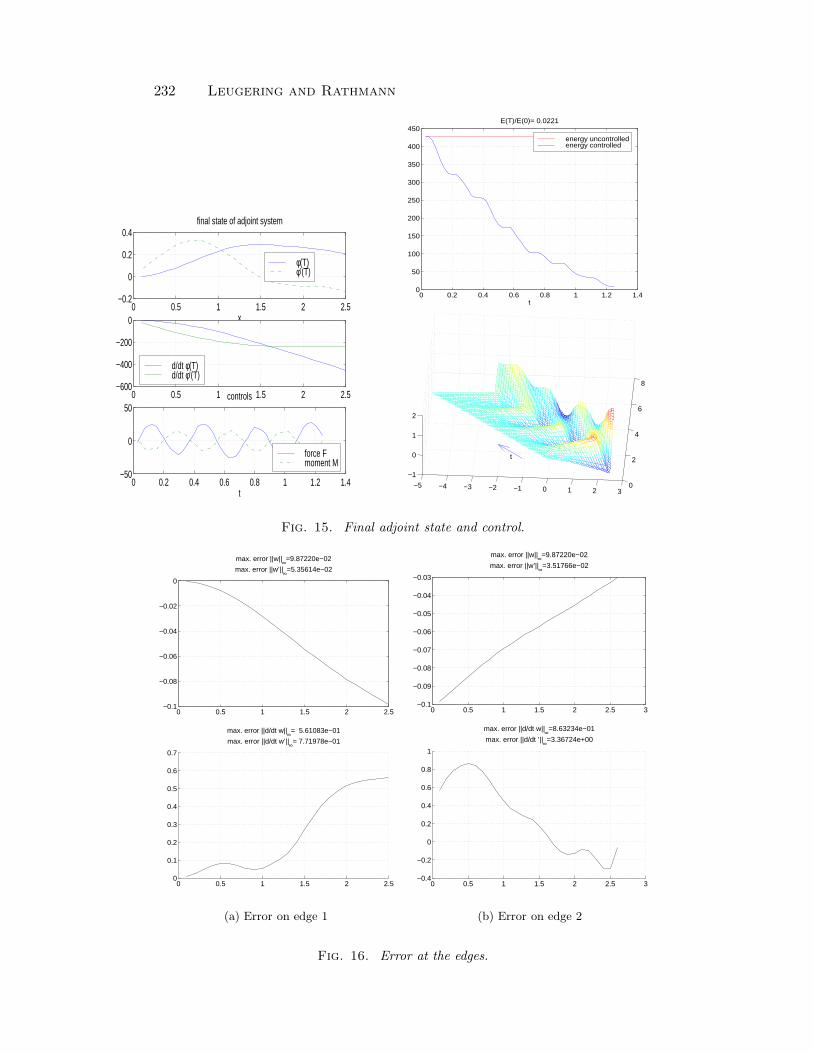
232 Leugering and Rathmann
0 0.5 1 1.5 2 2.5−0.2
0
0.2
0.4
x
final state of adjoint system
φ(T)φ’(T)
0 0.5 1 1.5 2 2.5−600
−400
−200
0
d/dt φ(T)d/dt φ’(T)
0 0.2 0.4 0.6 0.8 1 1.2 1.4−50
0
50
t
controls
force Fmoment M
0 0.2 0.4 0.6 0.8 1 1.2 1.40
50
100
150
200
250
300
350
400
450
t
E(T)/E(0)= 0.0221
energy uncontrolledenergy controlled
−5 −4 −3 −2 −1 0 1 2 30
2
4
6
8
−1
0
1
2
t
Fig. 15. Final adjoint state and control.
0 0.5 1 1.5 2 2.5−0.1
−0.08
−0.06
−0.04
−0.02
0
max. error ||w||∞=9.87220e−02
max. error ||w’||∞=5.35614e−02
0 0.5 1 1.5 2 2.50
0.1
0.2
0.3
0.4
0.5
0.6
0.7
max. error ||d/dt w||∞= 5.61083e−01
max. error ||d/dt w’||∞= 7.71978e−01
(a) Error on edge 1
0 0.5 1 1.5 2 2.5 3−0.4
−0.2
0
0.2
0.4
0.6
0.8
1
max. error ||d/dt w||∞=8.63234e−01
max. error ||d/dt ’||∞=3.36724e+00
0 0.5 1 1.5 2 2.5 3−0.1
−0.09
−0.08
−0.07
−0.06
−0.05
−0.04
−0.03
max. error ||w||∞=9.87220e−02
max. error ||w’||∞=3.51766e−02
(b) Error on edge 2
Fig. 16. Error at the edges.

Local Characterizations of Saddle Points and Their
Morse Indices
Yongxin Li , IBM Watson Research Center, Yorktown Hts, NYJianxin Zhou1, Texas A&M University, College Station, Texas.
Abstract
In this paper, numerically computable bound estimates of the Morseindices of saddle points are established through their new local minimaxtype characterizations. The results provide methods for measuringinstability of unstable solutions in system design and control theory.
1 Introduction
Let H be a Hilbert space and J : H → R be a Frechet differentiablefunctional. Denote by J ′ its Frechet derivative and J ′′ its second Frechetderivative if it exists. A point u ∈ H is a critical point of J if
J ′(u) = 0
as an operator J ′ : H → H. A number c ∈ R is called a critical value of Jif J(u) = c for some critical point u. For a critical value c, the set J−1(c)is called a critical level. When the second Frechet derivative J ′′ exists at acritical point u, u is said to be non-degenerate if J ′′(u) is invertible as a linearoperator J ′′(u) : H → H. Otherwise u is said to be degenerate. The firstcandidates for a critical point are the local maxima and minima to which theclassical critical point theory was devoted in calculus of variation. Traditionalnumerical methods focus on finding such stable solutions. Critical points thatare not local extrema are unstable and called saddle points, that is, criticalpoints u∗ of J , for which any neighborhood of u∗ in H contains points v,w s.t.J(v) < J(u∗) < J(w). In physical systems, saddle points appear as unstableequilibria or transient excited states.
1Supported in part by NSF Grant DMS 96-10076. E-mail: [email protected]
233

234 Li and Zhou
Assume that at a critical point u∗, J ′′(u∗) is a self-adjoint, Fredholmoperator from H → H, according to the spectral theory H has an orthogonalspectral decomposition
H = H− ⊕H0 ⊕H+
where H−,H0 and H+ are respectively the maximum negative definite, the nulland the maximum positive definite subspaces of J ′′(u∗) inH with dim(H0) <∞and, H−,H0 and H+ are closed invariant subspaces under J ′′(u∗). Followingthe Morse theory, the Morse index of the critical point u∗ of J is MI(u∗) =dim(H−). So for a non-degenerate critical point, if its MI = 0, then it is alocal minimizer and a stable solution, and if its MI > 0, then it is a min-maxtype and unstable solution. Throughout this paper, when the Morse index isinvolved, we always assume that at a critical point u∗, J ′′(u∗) is a self-adjoint,Fredholm operator from H → H. So the orthogonal spectral decomposition ofH will always be available.
When saddle points are introduced, one may mention another saddle pointapproach in optimization and game theory. Note that in optimization and gametheory, saddle points are defined differently. For given vector spaces X and Y ,let f : X×Y → R be a function. A saddle point of f is a point (x∗, y∗) ∈ X×Ysuch that there exist neighborhoods N (x∗) of x∗ in X and N (y∗) of y∗ in Ysatisfying
f(x∗, y) < f(x∗, y∗) < f(x, y∗) ∀ x ∈ N (x∗),∀ y ∈ N (y∗).
Such a saddle point is usually also a critical point of f in X×Y . The significantdifference here is that f has a splitting structure on X×Y and such a splittingstructure is known beforehand and fixed. Interactions between X and Y aretherefore very limited. While saddle points defined in critical point theoryare much more general. Such a splitting structure is in general not available.If u∗ ∈ H is a nondegenerate critical point of a generic energy function Jwith MI(u∗)/geq1, by the spectral theory, we have H = H− ⊕ H+. Then wehave the decomposition u∗ = u− + u+ for u− ∈ H−, u+ ∈ H+ and there areneighborhoods N (u−) of u− in H− and N (u+) of u+ in H+ such that
J(v + u+) < J(u− + u+) < J(u− + w) ∀v ∈ N (u−), w ∈ N (u+).
A formation close to a saddle point in optimization and game theory. However,here the splitting structure H = H−⊕H+ is only partial, interactions betweenH− and H+ are allowed. The most important difference here is that thesubspaces H− and H+ cannot be available before we physically find the saddlepoint u∗. Therefore such an approach plays little role in finding or searchingsaddle points in the critical point theory.
Multiple solutions with different performances and instabilities exist inmany nonlinear problems in natural and social sciences [22], [19], [14], [24],

Saddle Points and Their Morse Indices 235
[13]. Stability is one of the main concerns in system design and controltheory. For instance, traveling waves have been observed to exist in suspendedbridges-a nonlinear beam equation [6] and showed as saddle points, thereforeunstable solutions, to their corresponding variational problem ((10) and (11) in[6]). Those unstable solutions have been observed to have different instabilityproperties. How to mathematically measure their instability properties becomesan interesting problem. As matter of fact, travelling waves make up animportant class of solutions to both reaction-diffusion equation and nonlinearhyperbolic equations with “viscosity”. They are solutions of the form u =u(x−ct) where c is a constant, the speed of the wave. Many phenomena arising invarious physical, or biological context can be modelled by travelling waves; suchas shock waves, nerve impulses, and various oscillatory chemical reactions. Thenice mathematical feature associated with such solutions is that the problemoften reduces to a nonlinear ordinary differential equations and the solutionscorrespond to saddle points of their generic energy functions (ref. Chapter 24in [21]). Stability (instability) analysis of such solutions is interesting to manyengineers and researchers and has been carried out in the literature.
Our objective is to develop some mathematical tool to measure instabilityproperties for saddle points. Usually stability describes certain propertypossessed by a solution to a dynamic system. When one says that a solutionu∗ is a stable solution to a dynamic system, if u0 is near u∗, the solution tothe dynamic system through u0 tends to u∗ as t → +∞. One may show thata solution u∗ to a dynamic system is stable if the spectrum of the linearizedoperator of the dynamic system at u∗ lies in the left-hand complex plane. Whenthe system is variational, an associated energy function is available. One mayalso use the energy function to define stability. In this paper, we say that asolution (critical point) u∗ is stable if it is a local minimizer of the associatedgeneric energy function. In this case MI(u∗) = 0. Thus any local perturbation ofa stable solution in an associated feasible function space will increase the energylevel. For an unstable solution (saddle point) u∗, we may also use the maximumdimension of a subspace in which a local perturbation of the unstable solutionu∗ in an associated feasible function space will always decrease the energy levelto define its instability index. Since by the definition, any local perturbation ofu∗ in H− will always decrease its energy level, for such variational problems, theMorse index (= dim(H−)) of a solution can be used to measure its instability(ref. [4],[21]). It is clear that the Morse index serves as a lower bound of theinstability index. On the other hand, in many applications, performance ormaneuverability is more desirable, in particular, in system design or controlof emergency or combat machineries. Usually unstable solutions have muchhigher maneuverability or performance indices. For providing choice or balancebetween stability and maneuverability or performance, it is important to solvefor multiple solutions and their Morse indices. When a saddle point u0 is

236 Li and Zhou
degenerate, the nullspace H0 of J ′′(u0) is nonempty. Since many differentsituations may happy in H0, it is extremely difficult to determine the Morseindex in this case. On the other hand, whether or not a solution is degeneratealso depends on the domain of the solution. So we can not simply exclude suchsituation.
When cases are variational, we will be dealing with multiple critical pointproblems. So it is important for both theory and applications to numericallysolve for multiple critical points and their Morse indices in a stable way. So far,little is known in the literature to devise such a feasible numerical algorithm.Minimax principle is one of the most popular approaches in critical point theory.However, most minimax theorems in the literature (See [1], [16], [17], [19],[24]), such as the mountain pass, various linking and saddle point theorems,require one to solve a two-level global optimization problem and therefore notfor algorithm implementation.
In [11], motivated by the numerical works of Choi-McKenna [7] and Ding-Costa-Chen 9, the Morse theory and the idea to define a solution submanifold,new local minimax theorems which characterize critical points as solutions toa two-level local optimization problem are established. Based on the localcharacterization, a new numerical minimax method for finding multiple criticalpoints is devised. The numerical method is implemented successfully to solve aclass of semilinear elliptic PDE on various domains for multiple solutions [11].Although Morse index has been printed for each numerical solution obtained in[11], their mathematical verifications have not been established. In [2], by usinga global minimax principle, A. Bahri and P.L. Lions established some lowerbound estimates for the Morse indices of solutions to a class of semilinear ellipticPDE. There are also some efforts in the literature to numerically compute theMorse index of a solution to a class of semilinear elliptic PDE. In addition tofinding a saddle point, one has to solve a corresponding linearized elliptic PDEat the solution for its first a few eigen-values. It is very expensive and not muchsuccess has been documented.
Since Morse index reflects local structure of a critical point, in this paperwe show that our local minimax characterization enables us to establish moreprecise estimates for the Morse index of a saddle point in a more general setting.By our results the Morse index of a saddle point based on the local minimaxmethod can be estimated even before we numerically compute the saddle point.So no extra work is required in addition to computation for the saddle point.In the last section, new local characterization of saddle points which are moregeneral than minimax solutions and bound estimates for their Morse indiceswill be developed. In the rest of this section, we introduce some notations andtheorems from [11] for future use.
For any subspace H ′ ⊂ H, let SH′ = v|v ∈ H ′, ‖v‖ = 1 be the unitsphere in H ′. Let L be a closed subspace in H, called a base space, and
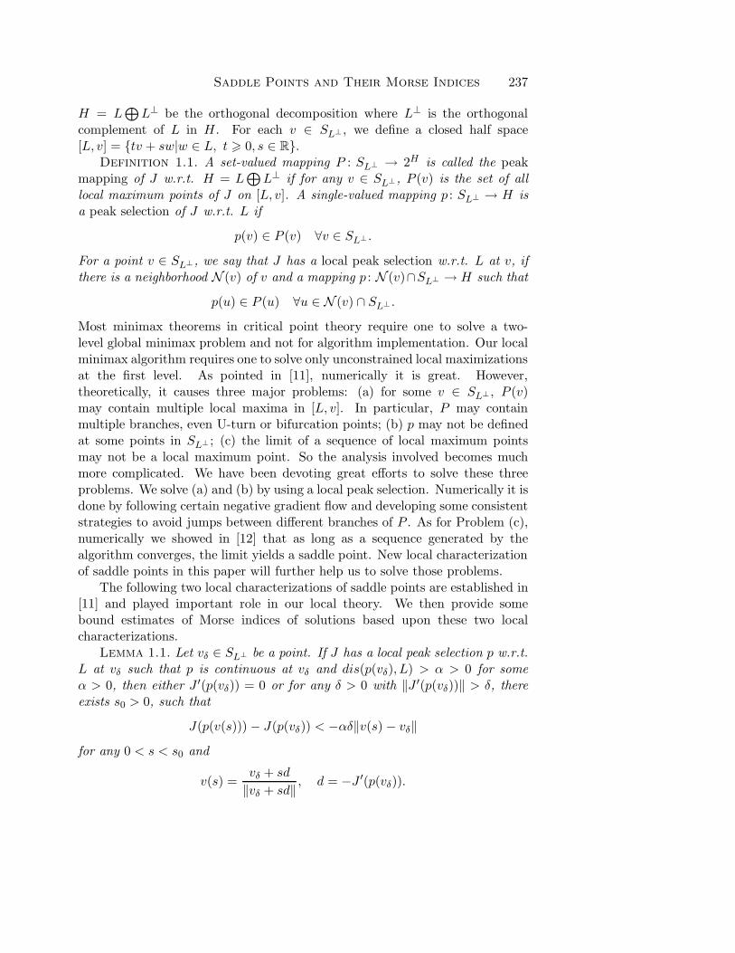
Saddle Points and Their Morse Indices 237
H = L⊕L⊥ be the orthogonal decomposition where L⊥ is the orthogonal
complement of L in H. For each v ∈ SL⊥ , we define a closed half space[L, v] = tv + sw|w ∈ L, t > 0, s ∈ R.
Definition 1.1. A set-valued mapping P : SL⊥ → 2H is called the peakmapping of J w.r.t. H = L
⊕L⊥ if for any v ∈ SL⊥ , P (v) is the set of all
local maximum points of J on [L, v]. A single-valued mapping p : SL⊥ → H isa peak selection of J w.r.t. L if
p(v) ∈ P (v) ∀v ∈ SL⊥ .
For a point v ∈ SL⊥, we say that J has a local peak selection w.r.t. L at v, ifthere is a neighborhood N (v) of v and a mapping p : N (v)∩SL⊥ → H such that
p(u) ∈ P (u) ∀u ∈ N (v) ∩ SL⊥ .
Most minimax theorems in critical point theory require one to solve a two-level global minimax problem and not for algorithm implementation. Our localminimax algorithm requires one to solve only unconstrained local maximizationsat the first level. As pointed in [11], numerically it is great. However,theoretically, it causes three major problems: (a) for some v ∈ SL⊥ , P (v)may contain multiple local maxima in [L, v]. In particular, P may containmultiple branches, even U-turn or bifurcation points; (b) p may not be definedat some points in SL⊥ ; (c) the limit of a sequence of local maximum pointsmay not be a local maximum point. So the analysis involved becomes muchmore complicated. We have been devoting great efforts to solve these threeproblems. We solve (a) and (b) by using a local peak selection. Numerically it isdone by following certain negative gradient flow and developing some consistentstrategies to avoid jumps between different branches of P . As for Problem (c),numerically we showed in [12] that as long as a sequence generated by thealgorithm converges, the limit yields a saddle point. New local characterizationof saddle points in this paper will further help us to solve those problems.
The following two local characterizations of saddle points are established in[11] and played important role in our local theory. We then provide somebound estimates of Morse indices of solutions based upon these two localcharacterizations.
Lemma 1.1. Let vδ ∈ SL⊥ be a point. If J has a local peak selection p w.r.t.L at vδ such that p is continuous at vδ and dis(p(vδ), L) > α > 0 for someα > 0, then either J ′(p(vδ)) = 0 or for any δ > 0 with ‖J ′(p(vδ))‖ > δ, thereexists s0 > 0, such that
J(p(v(s))) − J(p(vδ)) < −αδ‖v(s) − vδ‖
for any 0 < s < s0 and
v(s) =vδ + sd
‖vδ + sd‖ , d = −J ′(p(vδ)).

238 Li and Zhou
The above result indicates that v(s) defined in the lemma represents adirection for certain negative gradient flow of J(p(·)) from v. So it is clearthat if p(v0) is a local minimum point of J on any subset containing the pathp(v0(s)) for some small s > 0 then J ′(p(v0)) = 0. In particular, if we define asolution manifold
M =p(v) : v ∈ SL⊥
,
we have p(v(s)) ⊂ M. A solution submanifold was first introduced byNehari in study of a dynamic system [15] and then applied by Ding-Ni instudy of semilinear elliptic PDE [17]. Although their definitions of a solutionsubmanifold are closely related to the problems that they were dealing withand our definition of a solution submanifold is given in a quite general setting,it is easy to check that their solution submanifold coincides with ours withL = 0. While for our solution submanifold, L can be any closed subspace. Soour definition of a solution submanifold generalizes their notions. Furthermore,they prove that a global minimum point of the generic energy function J onthe solution submanifold M w.r.t. L = 0 yields a saddle point basically withMI= 1. While our next theorem proved in [11] shows that a local minimum pointof the generic energy function J on our solution submanifold M also yields asaddle point and the Morse index of such a saddle point can be greater thanone. Since for such an unstable saddle point u∗, its generic energy is minimizedon the corresponding solution submanifold, the solution submanifold becomesa stable submanifold of the unstable saddle point u∗, in the sense that anysmall perturbation of u∗ will increase the value of the generic functional J aslong as the perturbation stays on the submanifold M. Since u∗ is a saddlepoint, a perturbation of u∗ off the submanifold may decrease the value of thegeneric energy functional J . So the solution submanifold is also called a stablesubmanifold.
Theorem 1.1. [11] Let v0 ∈ SL⊥ be a point. If J has a local peak selectionp w.r.t. L at v0 s.t.
(i) p is continuous at v0,
(ii) dis(p(v0), L) > 0 and
(iii) v0 is a local minimum point of J(p(v)) on SL⊥.
Then p(v0) is a critical point of J .The following PS condition will be used to replace the usual compact
condition.Definition 1.2. A function J ∈ C1(H) is said to satisfy the Palais-Smale
(PS) condition, if any sequence un ∈ H with J(un) bounded and J ′(un) → 0has a convergent subsequence.
Saddle Points and Their Morse Indices 239
2 Bound Estimates for Morse Index
The Morse index provides understanding of the local structure of a saddle pointand is used as an instability index for an unstable solution [4],[21]. It is animportant notion in stability analysis [4]. Although we have printed the Morseindex for each numerical solution computed by our minimax method in [11],their mathematical justifications have not been verified. In this section, weestablish several bound estimates for the Morse index of a critical point basedon our minimax method.
Lemma 2.1. Let v0 ∈ SL⊥ be a point. If there exist a neighborhoodN (v0) of v0 and a locally defined mapping p : N (v0) ∩ SL⊥ → H such thatp(v) ∈ L, v ∀v ∈ N (v0)∩SL⊥ . If p is differentiable at v0 and u0 = p(v0) /∈ L,then
p′(v0)(L, v0⊥) + L, v0 = H.
Proof. For any w ∈ L, v0⊥, ‖w‖ = 1, denote vs =v0 + sw
‖v0 + sw‖ . Then there
exists s0 > 0 such that when |s| < s0, we have vs ∈ N (v0) ∩ SL⊥ .Consider the one dimensional vector function α(s) = PL⊥(p(vs)), where
PL⊥ is the projection onto L⊥. Since p is differentiable at v0 and vs smoothlydepends on s, α is differentiable at 0 and
α′(0) = PL⊥(p′(v0)(∂vs∂s
)) = PL⊥(p′(v0)(w)).
On the other hand, p(vs) ∈ L, vs, we have α(s) = tsvs, where ts = 〈α(s), vs〉is differentiable. So α′(0) = t′0v0 + t0w, where due to our assumption thatu0 = p(v0) /∈ L, we have t0 6= 0. The two different expressions of α′(0) imply
PL⊥(p′(v0)(w)) = t′s(0)v0 + t0w.
Then it leads to w ∈ p′(v0)(w), L, v0. Since w is an arbitrary vector inL, v0⊥, it follows that
L, v0⊥ ⊂ p′(v0)(L, v0⊥), L, v0
or
p′(v0)(L, v0⊥) + L, v0 = H.(2.1)
Lemma 2.2. Let v0 ∈ SL⊥ be a point. If there exist a neighborhoodN (v0) of v0 and a locally defined mapping p : N (v0) ∩ SL⊥ → H such thatp(v) ∈ L, v ∀v ∈ N (v0) ∩ SL⊥. Assume that p is differentiable at v0 andu0 = p(v0) /∈ L. If u0 is a critical point of J with MI(u0) > dimL+ 1, then
p′(v0)(L, v0⊥) ∩H− 6= 0.
240 Li and Zhou
Proof. Denote H− the negative subspace of J ′′(u0) and k = dimL + 1.Then dimH− > k. By applying Lemma 2.1, there exit linearly independentvectors e0, e1, . . . , ek ∈ H− which can be represented as ei = gi + fi withgi ∈ p′(v0)(L, v0⊥) and fi ∈ L, v0. f0, f1, . . . , fk have to be linearlydependent because k = dimL + 1. So we can find real numbers a0, a1, . . . , aksuch that
∑ki=0 a
2i 6= 0 and
∑ki=0 aifi = 0. Therefore
k∑i=0
aiei =k∑i=0
aigi ∈ p′(v0)(L, v0⊥) ∩H−.
Because, e0, e1, . . . , ek are linearly independent,∑k
i=0 aiei 6= 0. Thus, theconclusion of the lemma is verified.
Theorem 2.1. Let v0 ∈ SL⊥ be a point. If J has a local peak selection pw.r.t. L at v0 such that p is differentiable at v0 and u0 = p(v0) /∈ L. If v0 isa local minimum point of J p on SL⊥, then u0 is a critical point of J withMI(u0) 6 dimL+ 1.Proof. Since p is a local peak selection of J w.r.t. L at v0, there exists aneighborhood N (v0) of v0 such that p(v) ∈ L, v, ∀v ∈ N (v0) ∩ SL⊥ . Byapplying Lemma 2.1, we have
p′(v0)(L, v0⊥) + L, v0 = H
orcodim(p′(v0)(L, v0⊥)) 6 dimL+ 1.
Now suppose that MI(u0) > dimL+ 1. Denote H− the negative subspace ofJ ′′(u0). By Lemma 2.2, we have
p′(v0)(L, v0⊥) ∩H− 6= 0.(2.2)
Choose any w ∈ L, v0⊥, ‖w‖ = 1, such that p′(v0)(w) ∈ H−. Aroundu0 = p(v0), we have the second order Taylor expansion
J(u) = J(u0) +12〈J ′′(u0)(u− u0), u− u0〉 + o(‖u− u0‖2)(2.3)
Denote vs =v0 + sw
‖v0 + sw‖ , we have vs ∈ N (v0) ∩ SL⊥ for |s| small and then
dvsds
|s=0 = w. So it follows
p(vs) = u0 + sp′(v0)(w) + o(|s|).(2.4)
Combining the above two estimates (2.3) and (2.4), we obtain

Saddle Points and Their Morse Indices 241
J(p(vs))
= J(u0) +12〈J ′′(u0)(sp′(v0)(w) + o(|s|)), sp′(v0)(w) + o(|s|)〉
+o(‖sp′(v0)(w) + o(|s|)‖2)
= J(u0) +12s2〈J ′′(u0)(p′(v0)(w)), p′(v0)(w)〉 + o(s2)
< J(u0),
where the last strict inequality holds for |s| sufficiently small, becausep′(v0)(w) ∈ H−.
Since vs ∈ N (v0) ∩ SL⊥ and u0 = p(v0), the above contradicts theassumption that v0 is a local minimum point of J p on SL⊥ . ThereforeMI(u0) 6 dimL+ 1.
Theorem 2.2. If p is a local peak selection of J w.r.t. L at v0 ∈ SL⊥ andu0 = p(v0) is a nondegenerate critical point of J , then MI(u0) > dimL+ 1.Proof. Assume that k ≡ MI(u0) < dimL + 1. By our assumption, u0 isnondegenerate, i.e., J ′′(u0) is invertible, we have H = H+
⊕H− where H+
is the maximum positive subspace and H− is the maximum negative subspacecorresponding to the orthogonal spectral decomposition of J ′′(u0). It followsthat codim(H+) = dim(H−) = k < dimL + 1, so there exists a non-zerovector v ∈ H+ ∩ L, v0. When v ∈ H+, for sufficient small t, we haveJ(u0 + tv) > J(u0). But this contradicts to that u0 is a local maximum pointof J in the subspace L, v0. Therefore, MI(u0) > dimL+ 1.
Theorem 2.3. Assume that p is a local peak selection of J w.r.t. L atv0 ∈ SL⊥ such that p is differentiable at v0 and u0 = p(v0) /∈ L. If v0is a local minimum point of J p on SL⊥, and J ′′(u0) is invertible, thenMI(u0) = dimL+ 1.Proof. Since under the conditions, we have proved that u0 = p(v0) is a non-degenerate critical point of J . The conclusion follows by combining the last twotheorems.
Theorem 2.4. Let v0 ∈ SL⊥ be a point. If there exist a neighborhood N (v0)of v0 and a locally defined mapping p : N (v0)∩SL⊥ → H such that p(v) ∈ L, v,J ′(p(v)) ⊥ L, v, ∀v ∈ N (v0) ∩ SL⊥ and p differentiable at v0. If v0 ∈ SL⊥ isa local minimum point of J p on SL⊥ with u0 = p(v0) /∈ L, then u0 is a criticalpoint of J with MI(u0) 6 dimL+ 1.Proof. We first prove that u0 = p(v0) is a critical point of J . The second partof the theorem follows from a similar proof of Theorem 2.1.
For any w ∈ L, v0⊥, denote
v(s) =v0 + sw
‖v0 + sw‖ .

242 Li and Zhou
We have v(s) ∈ N (v0) ∩ SL⊥ for |s| small and dv(s)ds |s=0 = w. Therefore
p(v(s)) = p(v0) + sp′(v0)dv(s)ds
|s=0 + o(|s|)
= u0 + sp′(v0)(w) + o(|s|).
It follows that
J(p(v(s))) = J(p(v0)) + J ′(p(v0))(p(v(s)) − p(v0)) + o(‖p(v(s)) − p(v0)‖)= J(u0) + sJ ′(u0)p′(v0)(w) + o(|s|).
IfJ ′(u0)p′(v0)(w) 6= 0
for some w ∈ L, v0⊥, then when |s| is sufficiently small, we can choose eithers > 0 or s < 0 such that
J(p(v(s))) < J(p(v0))
which contradicts the assumption that v0 is a local minimum point of J p onSL⊥ . Thus
J ′(u0)p′(v0)(L, v0⊥) = 0.
Since by our assumptionJ ′(u0)(L, v0) = 0
and by Lemma 2.1p′(v0)(L, v0⊥) + L, v0 = H,
it follows thatJ ′(u0)u = 0 ∀u ∈ H,
i.e., u0 = p(v0) is a critical point of J .It is worthwhile indicating that if p is a local peak selection of J at v0 ∈ SL⊥ ,
then p(v) ∈ [L, v] and J ′(p(v)) ⊥ [L, v] for all v ∈ N (v0) ∩ SL⊥ . If vn ⊂ SL⊥ ,vn → v0 and un = p(vn) → u0, we have u0 ∈ [L, v0] and J ′(u0) ⊥ [L, v0]. Sosuch a locally defined mapping generalized the notion of a local peak selectionand resolved the problem that a limit of a sequence of local maximum pointsmay not be a local maximum point. This generalization has a potential todesign a new type of local algorithm for finding multiple saddle points that arenot necessarily of a minimax type.
Theorem 2.5. If u0 /∈ L is a non-degenerate critical point of J such thatu0 is not a local minimum point of J along any direction v ∈ L, u0, then
MI(u0) > dimL+ 1.

Saddle Points and Their Morse Indices 243
Proof. Assume that k = MI(u0) < dimL + 1. By our assumption, u0 is non-degenerate, i.e., J ′′(u0) is invertible, we have H = H+ ⊕ H− where H+ isthe maximum positive subspace and H− is the maximum negative subspacecorresponding to the orthogonal spectral decomposition of J ′′(u0). It followsthat codim(H+) = dim(H−) = k < dimL+1, so there exists a non-zero vectorv ∈ H+ ∩ L, u0. When v ∈ H+, for sufficiently small t, we have
J(u0 + tv) > J(u0).
It then contradicts the assumption that u0 is not a local minimum point of Jalong any direction v ∈ L, u0.
3 Application to Semilinear Elliptic PDEs
Semilinear elliptic boundary-value problems (BVP) are known to be rich inmultiple solutions. Some of the solutions are stable and others are unstable.How to measure the instability properties for unstable solutions is an interestingproblem, which is actually part of the motivation of this paper. When the profileof a solution shown as in Figure 1 was obtained and presented to the nonlinearpartial differential equation community, it generated warm debates about theexistence and the Morse index of such a solution. The authors are happy toknow that the existence issue has been recently settled [23]. But the Morseindex of such a solution is still unsolved. In this section, we try to answer thequestion.
Consider a semilinear elliptic Dirichlet BVP on a piecewise smooth boundeddomain Ω in R
n which has many applications in physics, engineering, biology,ecology, geometry, etc
∆u(x) + f(x, u(x)) = 0, x ∈ Ω,u(x) = 0, x ∈ ∂Ω,
(3.1)
where the function f(x, u(x)) satisfies the following standard hypothesis:
(h1) f(x, u(x)) is locally Lipschitz on Ω × R;
(h2) there are positive constants a1 and a2 such that
|f(x, ξ)| 6 a1 + a2|ξ|s(3.2)
where 0 6 s < n+2n−2 for n > 2. If n = 2,
|f(x, ξ)| 6 a1 exp φ(ξ)(3.3)
where φ(ξ)ξ−2 → 0 as |ξ| → ∞;
(h3) f(x, ξ) = o(|ξ|) as ξ → 0;

244 Li and Zhou
(h4) there are constants µ > 2 and r > 0 such that for |ξ| > r,
0 < µF (x, ξ) 6 ξf(x, ξ),(3.4)
where F (x, ξ) =∫ ξ0 f(x, t)dt.
(h4) says that f is superlinear, which implies that there exist positive numbersa3 and a4 such that for all x ∈ Ω and ξ ∈ R
F (x, ξ) > a3|ξ|µ − a4.(3.5)
The generic energy functional associated to the Dirichlet problem (3.1) is
J(u) =12
∫Ω|∇u(x)|2dx−
∫ΩF (x, u(x))dx, u ∈ H ≡ H1
0 (Ω),(3.6)
where we use an equivalent norm ‖u‖ =∫Ω |∇u(x)|2dx for the Sobolev space
H = H10 (Ω). It is well known [19] that under Conditions (h1) through (h4),
J is C1 and satisfy (PS) condition. A critical point of J is a weak solution,and also a classical solution of (3.1). 0 is a local minimum point of J and so atrivial solution. Moreover, in any finitely dimensional subspace of H, J goes tonegative infinity uniformly. Therefore, for any finite dimensional subspace L,the peak mapping P of J w.r.t. L is nonempty.
We need one more hypothesis, that is
(h5) f(x,ξ)|ξ| is increasing w.r.t. ξ, or
(h5’) f(x, ξ) is C1 w.r.t. ξ and fξ(x, ξ) − f(x,ξ)ξ > 0.
It is clear that (h5’) implies (h5). If f(x, ξ) is C1 in ξ, then (h5) and (h5’)are equivalent. All the power functions of the form f(x, ξ) = |ξ|kξ with k > 0,satisfies (h1) through (h5’), and so do all the positive linear combinations ofsuch functions. Under (h5) or (h5’), J has only one local maximum point in anydirection, or, the peak mapping P of J w.r.t. L = 0 has only one selection.In other words, P = p. The proof can be found in [17] and [14].
Theorem 3.1. Under the hypothesis (h1) through (h5), if the peak mappingP of J w.r.t. a finitely dimensional subspace L is singleton at v0 ∈ SL⊥ andfor any v ∈ SL⊥ around v0, a peak selection p(v) is a global maximum point ofJ in [L, v], then p is continuous at v0.Proof. See [11].
Theorem 3.2. Assume that Conditions (h1) – (h5’) are satisfied and thatthere exist positive constants a5 and a6 s.t.
|fξ(x, ξ)| 6 a5 + a6|ξ|s−1(3.7)
where s is specified in (h2). Then the only peak selection p of J w.r.t. L = 0is C1.

Saddle Points and Their Morse Indices 245
Proof. See [11].Since w0 = 0 is the local minimum point of J and along each direction
v ∈ H, J has only one maximum point p(v), we have J(p(v)) > 0,∀v ∈ S. Iffor each v ∈ SL⊥ , p(v) is a local maximum point of J in [L, v], then p(v) is theonly local maximum point of J along the direction u = p(v)
‖p(v)‖ , Therefore wehave J(p(v)) > 0,∀v ∈ SL⊥ . As a composite function J(p(·)) is bounded frombelow by 0. So Ekeland’s variational principle can be applied. With the PScondition, existence result can also be established.
Theorem 3.3. Under the hypothesis of (h1) through (h5), and that thereexist positive constants a5 and a6 such that
|fξ(x, ξ)| 6 a5 + a6|ξ|s−1,
where s is specified in (h2), if v0 = arg minv∈SHJ(p(v)) then u0 = p(v0) is a
critical point with MI(u0) = 1.Proof. Assume u0 = p(v0) = t0v0. Consider the 1-dimensional function
g(t) = J(tv0) =12
∫Ωt2|∇v0(x)|2 dx−
∫ΩF (x, tv0(x)) dx.
We haveg′(t) = t
∫Ω|∇v0(x)|2 dx−
∫Ωf(x, tv0(x))v0(x) dx.
So1 =
∫Ω
f(x, t0v0(x))t0v0(x)
v20(x) dx.
Meanwhile we have
g′′(t) =∫
Ω|∇v0(x)|2 dx−
∫Ωfξ(x, tv0(x))v2
0(x) dx
g′′(t0) = 1 −∫
Ωfξ(x, t0v0(x))v2
0(x) dx
< 1 −∫
Ω
f(x, t0v0(x))t0v0(x)
v20(x) dx (ref. (h5))
= 0,
which implies thatH0 ∩ L, v0 = 0,
where H0 is the nullspace of the linear operator J ′′(u0) and L = 0, i.e.,J ′′(u0) may be degenerate, however its restriction to the direction of v0 will notbe degenerate, where u0 = t0v0 is a critical point. By Theorem 2.1, we obtain
MI(u0) = dim(L) + 1 = 1.

246 Li and Zhou
In the rest of this section, we display a numerical solution of (3.1) wheref(x, u(x)) = u3(x) and the domain Ω is the dumbbell shaped domain as shownin the lower part of Figure 1. It can be checked that all the assumptions(h1) − (h5) are satisfied. So the results in this section can be applied.Many unstable solutions to this problem has been numerically computed anddocumented in [11]. The details of the numerical minimax method and howto compute such solutions are described in [11]. Some convergent properties ofthis numerical minimax method are established in [12]. Here we only displaythe profile and the contours the solution concentrated near the center of thecorridor of the dumbbell-shaped domain. This solution is also captured byusing a different numerical algorithm in [5]. It is this solution that generatedwarm debates about the existence and the Morse index of such a solution. SinceL = 0, by the results in this section, we can now conclude that the Morseindex of this solution is one.
4 Some New Saddle Point Theorems
As our convergence results in [12] indicate that our algorithm can be used to finda non-minimax critical point, e.g., a Monkey saddle point. Thus the argumentalready exceeded the scope of a minimax approach. So far the only results wefound in the critical point literature which are more general than a minimaxprinciple are two theorems proved by S. I. Pohozaev in [10] or [18]. The followingresults are interesting generalizations. The first one is an embedding result.It is general but lacks of characterization. The second result has potentialapplications in devising a new numerical algorithm.
Theorem 4.1. Given L = spanw1, ..., wk in H and let
J(t, v, t1, .., tk) ≡ J(tv + t1w1 + ...+ tkwk).
If (t∗0, v∗, t∗1, .., t
∗k) is a conditional critical point of J subject to v ∈ SL⊥ with
t∗ 6= 0, then t∗0v∗ + t∗1w1 + ...+ t∗kwk is a critical point of J .
Proof. By the Lagrange Multiplier Theorem, there exist λ, µ, η1, .., ηk withλ2 + µ2 + η2
1 + ...+ η2k 6= 0 such that the Lagrange functional
L(t, v, t1, ..., tk) = λJ(t, v, t1, ..., tk) + µ‖v‖ +k∑i=1
ηi〈wi, v〉
has a critical point at (t∗0, v∗, t∗1, .., t
∗k). So we have

Saddle Points and Their Morse Indices 247
X
Y
Z
w−
axis
−5
0
10
15
y−axis
−1
0
1
x−axis
−1.5−10123
−1.5 −1 0 1 2 3−1
0
1
x−axis
y−ax
is 0.5511.1
1.65
2.22.76
3.31
3.86
4.96
5.51
6.61
Fig. 1. The profile of a positive solution and its contours with J = 159.0 andumax = 13.63.

248 Li and Zhou
∂L∂t
= 0 ⇒ λJt(t∗0, v∗, t∗1, ..., t
∗k) = 0;(4.1)
∂L∂v
= 0 ⇒ λJ ′v(t
∗0, v
∗, t∗1, ..., t∗k) + µ‖v∗‖′ +
k∑i=1
ηiwi = 0;(4.2)
∂L∂ti
= 0 ⇒ λJ ′ti(t
∗0, v
∗, t∗1, .., t∗k) = 0 or
λ〈J ′(t∗0v∗ + t∗1w1 + ...+ t∗kwk), wi〉 = 0, (i = 1, .., k).(4.3)
From (4.2), we have
〈λJv(t∗0, v∗, t∗1, .., t∗k), v〉 + µ〈‖v∗‖′, v〉 +k∑i=1
ηi〈wi, v〉 = 0 ∀v ∈ H.
(4.4)
In particular
λ〈Jv(t∗0, v∗, t∗1, .., t∗k), v∗〉 + µ〈‖v∗‖′, v∗〉 +k∑i=1
ηi〈wi, v∗〉 = 0.(4.5)
Since 〈‖v∗‖′, v∗〉 = 1 and 〈wi, v∗〉 = 0 for i = 1, ..., k, we obtain
λ〈Jv(t∗0, v∗, t∗1, .., t∗k), v∗〉 + µ = 0.(4.6)
So λ = 0 will lead to µ = 0 and then ηi = 0 by choosing v = wi in (4.3). Itcontradicts to λ2 + µ2 + η2
1 + ...+ η2k 6= 0. Therefore λ 6= 0 and (4.1) gives
J ′t(t
∗0, v
∗, t∗1, ..., t∗k) = 0
or〈J ′(t∗0v
∗ + t∗1w1 + ...+ t∗kwk), v∗〉 = 0.
It leads to
〈J ′v(t
∗0, v
∗, t∗1, ..., t∗k), v
∗〉 = t∗0〈J ′(t∗0v∗ + t∗1w1 + ...+ t∗kwk), v
∗〉= 0.
(4.6) then yields µ = 0. Taking any v ⊥ [w1, ..., wk] in (4.4), we obtain
λ〈J ′v(t
∗0, v
∗, t∗1, ..., t∗k), v〉 = 0
ort∗0〈J ′(t∗0v
∗ + t∗1w1 + ...+ t∗kwk), v〉 = 0.

Saddle Points and Their Morse Indices 249
Since t∗0 6= 0, it leads to
〈J ′(t∗0v∗ + t∗1w1 + ...+ t∗kwk), v〉 = 0 ∀v ⊥ [w1, ..., wk ].
Taking (4.3) into account, we have
〈J ′(t∗0v∗ + t∗1w1 + ...+ t∗kwk), u〉 = 0 ∀u ∈ H
orJ ′(t∗0v
∗ + t∗1w1 + ...+ t∗kwk) = 0.
So u∗ = t∗0v∗ + t∗1w1 + ...+ t∗kwk is a critical point.
It is clear that Theorem 4.1 reduces to Pohozaev’s embedding result in [10]or [18] if we set L = 0, the trivial subspace.
Theorem 4.2. Let v∗ ∈ SL⊥ be a point. If J has a local peak selection pw.r.t. L at v∗ and u∗ = p(v∗) such that
(i) p is Lipschitz continuous at v∗,
(ii) dis(u∗, L) > 0,
(iv) u∗ is a conditional critical point of J on p(SL⊥),
then u∗ is a critical point of J .Proof. Suppose that ‖J ′(u∗)‖ > 0. Set δ = 1
2‖J ′(u∗)‖. By Lemma 1.1, thereexists s0 > 0 such that
J(p(v∗(s))) − J(p(v∗)) < −δdis(u∗, L)‖v∗(s) − v∗‖ ∀0 < s < s0
wherev∗(s) =
v∗ + sd
‖v∗ + sd‖ ∈ N (v∗) ∩ SL⊥ , d = −J ′(p(v∗)).
Then we have
J(p(v∗(s))) − J(p(v∗))‖p(v∗(s)) − u∗‖
‖p(v∗(s)) − u∗‖‖v∗(s) − v∗‖ < −δdis(u∗, L), ∀ 0 < s < s0,(4.7)
where N (v∗) is a neighborhood of v∗ in which the local peak selection p isdefined. Since p is Lipschitz continuous at v∗ and u∗ is a conditional criticalpoint of J on p(SL⊥),
‖p(v∗(s)) − u∗‖‖v∗(s) − v∗‖
is bounded andJ(p(v∗(s))) − J(p(v∗))
‖p(v∗(s)) − u∗‖ → 0 as s→ 0.
So the left hand side of (4.7) goes to zero, which leads to a contradiction.

250 Li and Zhou
Theorem 4.3. Let v0 ∈ SL⊥ be a point. If J has a local peak selectionp w.r.t. L such that p is differentiable at v0 and u0 = p(v0) /∈ L. If u0 is aconditional critical point of J on p(SL⊥) and v0 is not a local maximum pointof J p along the projection of any direction v on SL⊥, then u0 is a criticalpoint of J with MI(u0) 6 dimL+ 1. In addition, if u0 is nondegenerate, thenMI(u0) = dimL+ 1.Proof. By Theorem 4.2, we obtain that u0 is a critical point of J . Then followinga similar argument in the proof of Theorem 2.1, until we have
J(p(vs)) = J(u0) +12〈J ′′(u0)(sp′(v0)(w) + o(|s|)), sp′(v0)(w) + o(|s|)〉
+o(‖sp′(v0)(w) + o(|s|)‖2)
= J(u0) +12s2〈J ′′(u0)(p′(v0)(w)), p′(v0)(w)〉 + o(s2)
< J(u0),
where
vs =v0 + sw
‖v0 + sw‖ ∈ N (v0) ∩ SL⊥ , w ∈ [L, v0]⊥, ‖w‖ = 1, and p′(v0)(w) ∈ H−.
So the last strict inequality contradicts to our assumption that v0 is not alocal maximum point of J p along the projection of any direction v on SL⊥ .Thus MI(u0) 6 dimL + 1. If in addition, u0 is nondegenerate, we can applyTheorem 2.5 to conclude that MI(u0) = dimL+ 1.
Condition (iv) in Theorem 4.2 is clearly satisfied if w∗ is a local minimumpoint of J on the solution (stable) manifold M = p(SL⊥). So it is clear thatTheorems 4.1 and 4.2 are indeed more general than a minimax principle. Asmatter of fact, Condition (iv) in Theorems 4.2 can be weekend as that w∗ isa conditional critical point of J on any subset containing the path p(v∗(s)) forsmall s > 0.
If we set L = 0, the trivial subspace and assume p(v) is the globalmaximum point of J on [L, v] = tv : t > 0 for each v ∈ SL⊥ = SH andp is C1, then Theorem 4.2 reduces to a result of Pohozaev in [18]. As we didin our algorithm, by gradually expanding the subspace L, Theorem 4.2 can beused to provide us with information on the Morse index of the critical point.For an example, when we solve a semilinear elliptic equation as shown in [11],we start from the trivial solution and set L = 0 to approximate a solution w1
with MI= 1; then we set L = w1 to search for a solution w2 with MI= 2,....This is the advantage of our approach.
As we can see in the above theorems, it becomes very important to checkwhether or not the local peak selection p is continuous or differentiable at v∗.This is very difficult at this stage, since an explicit expression of the local peakselection is not available. We are happy that we have found a solution. We

Saddle Points and Their Morse Indices 251
can embed a local peak selection into a more general local selection and thenuse the implicit function theorem to check whether or not the generalized localselection is differentiable at v∗. Finally we prove that if a local peak selection pcoincides with the more general local selection at v∗, then p is also differentiableat v∗. To apply the implicit function theorem, we only have to check whether ornot the determinant of an nxn matrix, where n = dim(L), is equal to zero. Thiscan be numerically carried out. This study has led to new approach, detailswill be presented in a future paper.
References
[1] A. Ambrosetti and P. Rabinowitz, Dual variational methods in critical pointtheory and applications, J. Funct. Anal. 14(1973), 349-381.
[2] A. Bahri and P.L. Lions, Morse index of some min-max critical points. I.Application to multiplicity results, Comm. Pure Appl. Math., Vol. XLI (1988)1027-1037.
[3] H. Brezis and L. Nirenberg, Remarks on Finding Critical Points, Comm. PureAppl. Math., Vol. XLIV, (1991), 939-963.
[4] K.C. Chang, Infinite Dimensional Morse Theory and Multiple Solution Problems,Birkhauser, Boston, 1993.
[5] G. Chen, W. Ni and J. Zhou, Algorithms and Visualization for Solutions ofNonlinear Elliptic Equations Part I: Dirichlet Problems, Int. J. Bifurcation &Chaos, to appear.
[6] Y. Chen and P. J. McKenna, Traveling waves in a nonlinearly suspended beam:Theoretical results and numerical observations, J. Diff. Equ., 136(1997), 325-355.
[7] Y. S. Choi and P. J. McKenna, A mountain pass method for the numericalsolution of semilinear elliptic problems, Nonlinear Analysis, Theory, Methods andApplications, 20(1993), 417-437.
[8] W.Y. Ding and W.M. Ni, On the existence of positive entire solutions of asemilinear elliptic equation, Arch. Rational Mech. Anal., 91(1986) 238-308.
[9] Z. Ding, D. Costa and G. Chen, A high linking method for sign changing solutionsfor semilinear elliptic equations, Nonlinear Analysis, 38(1999) 151-172.
[10] I. Kuzin and S. I. Pohozaev, Entire Solutions of Semilinear Elliptic Equations,Birkhauser, Boston, 1997.
[11] Y. Li and J. Zhou, A minimax method for finding multiple critical points and itsapplications to semilinear PDE, SIAM J. on Scientic Computing, to appear.
[12] Y. Li and J. Zhou, Convergence Results of a minimax method for finding multiplecritical points, submitted.
[13] F. Lin and T. Lin, “Minimax solutions of the Ginzburg-Landau equations”, SlectaMath. (N.S.), 3(1997) no. 1, 99-113.
[14] J. Mawhin and M. Willem, Critical Point Theory and Hamiltonian Systems,Springer-Verlag, New York, 1989.
[15] Z. Nehari, On a class of nonlinear second-order differential equations, Trans.Amer. Math. Soc., 95(19960), 101-123.
[16] W.M. Ni, Some Aspects of Semilinear Elliptic Equations, Dept. of Math. NationalTsing Hua Univ., Hsinchu, Taiwan, Rep. of China, 1987.

252 Li and Zhou
[17] W.M. Ni, Recent progress in semilinear elliptic equations, in RIMS Kokyuroku679, Kyoto University, Kyoto, Japan, 1989, 1-39.
[18] S. I. Pohozaev, On an approach to nonlinear equations, Dokl. Akad. Nauk SSSR,247(1979), 1327-1331;
[19] P. Rabinowitz, Minimax Method in Critical Point Theory with Applications toDifferential Equations, CBMS Regional Conf. Series in Math., No. 65, AMS,Providence, 1986.
[20] M. Schechter, Linking Methods in Critical Point Theory, Birkhauser, Boston,1999.
[21] J. Smoller, Shock Waves and Reaction-Diffusion Equations, Springer-Verlag, NewYork, 1982.
[22] M. Struwe, Variational Methods, Springer, 1996.[23] J. Wei and L. Zhang, “On the effect of the domain shape on the existence of large
solutions of some superlinear problems”, preprint.[24] M. Willem, Minimax Theorems, Birkhauser, Boston, 1996.

Static Buckling in a Supported Nonlinear Elastic
Beam
David L. Russell, Virginia Polytechnic Institute and State University,Blacksburg, VALuther W. White, University of Oklahoma at Norman, Norman, OK
Abstract
In the present paper we study finite static buckling effects in a nonlin-ear elastic beam supported on a flat, rigid, inelastic surface and subject toa gravitational force. We obtain necessary conditions characterizing equi-librium states as minima of the corresponding potential energy expressionand we show that we can obtain closed form expressions for the displace-ment of the beam above the supporting surface on intervals where thatdisplacement is positive.
AMS-MOS Classifications: 35J25, 35J50, 35Q72, 49L10; Keywords: nonlinearbeam, supported beam, buckling, constrained equilibrium
1 Introduction
In a recent article [6] the authors have studied buckling phenomena in thecontext of a nonlinear beam model originally introduced by Lagnese [2]. Ourpurpose in the present article is to revisit this model in a constrained situationwherein the beam is supported on a flat, rigid, inelastic surface – so that the onlypermissible transverse displacements are positive – and is subject to a uniformnegative force, which can be interpreted as gravity. A variety of applicationsoccur in circumstances where a strip of material, e.g., a track or a roadbed, islaid out over a supporting surface and may be subject to buckling away from thesupporting surface as a consequence of temperature-induced horizontal stresses,fast moving loads, etc..
We consider, then, an elastic beam of length L, with uniform cross section,in a two dimensional geometric context. The longitudinal extent of the beamcorresponds to the interval 0 ≤ x ≤ L and the beam is assumed to havethickness 2h. It will be convenient to suppose that in equilibrium the elasticaxis coincides with the x-axis, even though, strictly speaking, that violatesthe constraints described in the preceding paragraph. The displaced elastic
253
254 Russell and White
axis, or ”neutral curve”, admitting both transverse and lateral displacements,is described by (
xy
)−→
(x+ ξ(x)η(x)
), x ∈ [0, L],
where, minimally, ξ ∈ H1[0, L] and η ∈ H2[0, L]; in many cases we will needto assume more smoothness than this. The support constraint corresponds tothe condition η(x) ≥ 0. Assuming that linear material elements orthogonal tothe elastic axis in equilibrium remain so under admitted displacements, sucha deformation results in an infinitesimal stretching or contraction of materialfilaments parallel to the elastic axis having vertical coordinate y in equilibrium,with resultant arclength increment, using ′ to denote differentiation with respectto x,
ds =√
(1 + ξ′)2 + (y η′)2 dx.(1.1)
With the basic assumption, described in [6], to the effect that ξ and ξ′
are ofthe same order as η2, (η
′)2 and (η
′′)2, and, further, that these three are of the
same order as the thickness of the beam, discarding terms of higher order oneobtains, again as in [6], the potential energy expression for the beam in theform
V(ξ, η) =A
2
∫ L
0
(2ξ
′+(η′)2)2
dx +Bh2
6
∫ L
0
(η′′)2
dx
+ g
∫ L
0η(x) dx − κ ξ(L).(1.2)
Here g > 0 is the constant gravitational force acting in the negative y directionand κ > 0 represents a horizontal compressional force acting at the right(horizontally free) end of the beam; the left end of the beam is assumedhorizontally fixed so that ξ(0) = 0. The beam is assumed “transverselyclamped” at the endpoints x = 0 and x = L in the sense that η(x) and η
′(x)
vanish there; we formalize these requirements in §2 to follow. The positiveconstants A and B involve the elastic constants of the beam material and itswidth (in the third dimension which does not concern us here). All constantsshown here include, implicitly, a factor 2h corresponding to beam thickness(for example, the gravitational force is, for constant material mass density,proportional to beam thickness).
In §2, to follow, we establish the existence of a minimizer of the potentialenergy functional (1.2) under certain restrictions on the parameters of theproblem, as made precise in §6. In §3 we continue to develop necessaryconditions characterizing such a minimum. The purpose of §4 is to presenttwo detailed examples to clarify the results presented in §3. In §5 we carry

Static Buckling in a Supported Nonlinear Elastic Beam 255
out explicit computations resulting in analytic expressions for the solution incertain restricted circumstances. Finally, §6 serves as an appendix, establishingcertain bounds required in the work of §2.
2 Existence of a Potential Energy Minimizer
In this section we study the static equilibrium problem for the supported elasticbeam introduced in §1. Such an equilibrium is characterized as a minimizer ofthe potential energy expression V(ξ, η) given by (1.2) subject to the positivityconstraint
η(x) ≥ 0, x ∈ [0, L].(2.1)
We further suppose that the beam is “clamped” at the endpoints x = 0 andx = L; i.e., we have the boundary conditions (using
′to indicate differentiation
with respect to x)
η(0) = η′(0) = η(L) = η
′(L) = 0.(2.2)
We assume the left endpoint of the beam is horizontally fixed, correspondingto
ξ(0) = 0(2.3)
but we place no constraint on the horizontal right hand endpoint displacement;thus ξ(L) is free. These general boundary conditions are distinct from certainfree boundary conditions which we will need to introduce later in order tocharacterize intervals in which the minimizer component η(x) > 0.
A rigorous study of the potential energy minimization problem requires,first of all, a definition of appropriate “state spaces”. We let
V = H20 [0, L](2.4)
and define the subset corresponding to the imposed constraint as
V+ = η ∈ V | η(x) ≥ 0 .
We further define
U =ξ ∈ H1[0, L]
∣∣ ξ(0) = 0 (2.5)
and
X = U × V =χ ≡
(ξη
)ξ ∈ U, η ∈ V
;(2.6)
X+ = U × V+.

256 Russell and White
Expanding the potential energy in the form
V(ξ, η) =∫ L
0
2A(ξ′)2
+Bh2
6
(η′′)2dx + 2A
∫ L
0ξ′ (η′)2
dx
+A
2
∫ L
0
(η′)4
dx +∫ L
0g η dx + κ ξ(L),(2.7)
we designate the first term as the bilinear form a : X× X 7−→ R defined by
a(χ1, χ2) =∫ L
0
4Aξ
′1 ξ
′2 +
Bh2
3η′′1 η
′′2
dx.(2.8)
It is clear that a satisfies, for some positive numbers γ0, γ1, the coercivity andboundedness relations
γ0 ‖χ‖2X ≤ a(χ, χ), |a(χ1, χ2)| ≤ γ1 ‖χ1‖X‖χ2‖X.
We further define the nonlinear functional G : X 7−→ R by
G(χ) = 2A∫ L
0ξ′ (η′)2
dx.(2.9)
Defining W = W 1,40 [0, L] with norm ‖η‖ =
[∫ L0
(η′)4dx
] 14
; we observe that
|G(χ)| ≤ 2A ‖ξ′‖L2 ‖η‖2W ≤ 2A ‖ξ‖U ‖η‖2
W.
Using the definitions of the previous paragraph, we may express thepotential energy as
V(χ) =12a(χ, χ) + G(χ) +
A
2‖η‖4
W +∫ L
0g η dx + κ ξ(L).
For ε > 0 we introduce the perturbed form
Vε(χ) =12
(1 + ε) a(χ, χ) + G(χ) +A
2‖η‖4
W +∫ L
0g η dx + κ ξ(L),
(2.10)
for which we have the lower bound
Vε(χ) ≥ 12(1 + ε)
∫ L
0
(4A(ξ′)2
+Bh2
3
(η′′)2)dx
− 2A(∫ L
0
(ξ′)2
dx
) 12(∫ L
0
(η′)4
dx
) 12
+A
2‖η‖4
W +∫ L
0g η dx + κ ξ(L)

Static Buckling in a Supported Nonlinear Elastic Beam 257
≥ 12(1 + ε)
∫ L
0
(4A(ξ′)2
+Bh2
3
(η′′)2)dx − A
12
(4A∫ L
0
(ξ′) 1
2
)‖η‖2
W
+A
2‖η‖4
W +∫ L
0g η dx + κ ξ(L) ≥ 1
2(1 + ε) a(χ, χ)
−A12 a(χ, χ)
12‖η‖2
W +A
2‖η‖4
W − β0 g L12‖η‖V − κL
12 ‖ξ‖U.
Here we have used, for ξ(x) =∫ x0 ξ
′(x) dx,
| ξ(x)| ≤∫ x
0| ξ′(s)| dx ≤
(∫ x
0dx
) 12(∫ x
0| ξ′(s)|2 dx
) 12
⇒ | ξ(x)| ≤ x12 ‖ξ‖U, x ∈ [0, L],(2.11)
and, also, the estimates∫ L
0η dx ≤
(∫ L
0dx
) 12(∫ L
0η2 dx
) 12
≤ β0 L12 ‖η‖V,
‖η‖L2[0,l] ≤ β0 ‖η‖V, η ∈ V.
As a consequence we have
Vε ≥ ε
2a(χ, χ) − β0 g L
12 ‖η‖V − κL
12 ‖ξ‖U ≥ ε
2a(χ, χ)
−L12
(β0 g
2 + κ2) 1
2 ‖χ‖X ≥ ε γ0
2‖χ‖2
X − L12
(β0 g
2 + κ2) 1
2 ‖χ‖X.(2.12)
We now consider the regularized problem
Pε :
Minimize Vε(χ);χ ∈ X+.
.
From (2.12) we conclude that there exists an M0 such that
Vε(χ) ≥ M0(2.13)
and, for χ satisfying Vε(χ) ≤ M1 there exists M2 such that
‖χ‖X ≤ M2.(2.14)
Let χn be a minimizing sequence for Vε in X+; thus
Vε(χn) −→ d ≡ infχ∈X+
Vε(χ).

258 Russell and White
From (2.14) it is clear that χn is bounded in X. Thus there is asubsequence, which we still denote by χn , converging weakly in X to anelement χ ∈ X+, since X+ is weakly closed. In particular the correspondingsubsequence ηn converges weakly to η ∈ V. Since V embeds compactlyin W we may extract a further subsequence, which we continue to call ηn ,converging strongly to η in W which, further, implies
‖ηn‖W −→ ‖η‖W.
We may now conclude, since the correspondingξ′n
converges weakly to ξ in
L2[0, L] and(
η′n
)2
converges strongly to(η′)2
in L2[0, L], that
G(χn) = 2A∫ L
0ξ′n
(η′n
)2dx −→ 2A
∫ L
0ξ′ (η′)2
dx = G(χ).
It follows thatd = lim inf Vε(χn) ≥ Vε(χ)
and we conclude that there exists an element, which we will now call χε, suchthat
Vε(χε) = minχ∈X+
Vε(χ).
Now let us suppose that, possibly with some restrictions on the parametersof our problem, we can show that the set of ε-minima
χε∣∣ ε > 0
⊂ X+ is
bounded in X. Then, as ε −→ 0, a subsequence ηεk converges weakly in
V to some η 0 ∈ V+ and, passing to a further subsequence if necessary, ξεk
converges weakly in U to an element ξ0, which implies
lim inf a(χε, χε) ≥ a(χ0, χ0).
Let χ ∈ X+. Then
Vε(χ) =12(1 + ε)a(χ, χ) + G(χ) +
A
2‖η‖4
W + (g, η)L2[0,L] + κ ξ(L)
≥ Vε(χε) ≥ 12(1+ ε) a(χε, χε) + G(χε) +
A
2‖ηε‖4
W + (g, ηε)L2[0,L] + κ ξε(L).
In the limit as ε −→ 0 we have
V(χ) ≥ 12a(χ0, χ0) + G(χ0) +
A
2‖η 0‖4
W + (g, η 0)L2[0,L] + κ ξ0(L),
since it is clear that limε→ 0 Vε(χ) = V(χ). Then we have the desired result:
V(χ) ≥ V(χ0), χ ∈ X+.

Static Buckling in a Supported Nonlinear Elastic Beam 259
Thus the existence of a (not necessarily unique) minimizer for V is established.The proof of the boundedness of the χε is somewhat complicated; we leave it
for §6, which serves as an appendix, at the end of this paper. That proof requiressome restrictions on the parameters of the problem which may or may not berealistic in some cases. The proof given above is, of course, valid whenever wehave a uniform bound on the χε, whether or not that boundedness is obtainedas in §6.
3 General Conditions Characterizing a Minimizing Element
We begin this section with a choice of some minimizing element for V, as shownto exist in the previous section and there identified as χ0. Here we will referto such an element as χ and we will primarily be dealing with its individualcomponents ξ and η. We have the potential energy form (1.2) and the generalboundary conditions (2.2) and (2.3). We impose the positivity constraint (2.1)and we continue to use the spaces U, V and X as in (2.5), (2.4) and (2.6),respectively.
Let Y = Hp0 [0, L] for 1
2 < p ≤ 2; we define Z = U×Y and the mappingF : Z 7−→ Y by
F (ξ, η) = − η.
The restriction on p guarantees Hp0 [0, L] → C0[0, L] and thus that Y has
a positive cone Y+, corresponding to η(x) ≥ 0, x ∈ [0, L] with non-emptyinterior corresponding to η(x) > 0, x ∈ [0, L].
Applying an infinite dimensional version of the Kuhn-Tucker theorem [4],[5]there is an element λ ∈ Y∗ = H−p[0, L] such that the Lagrangian, defined by
L(χ, λ) = V(χ) + 〈λ, F (χ)〉 ,
has a stationary point at the solution of the minimization problem
minF (χ)≤ 0
V(χ).
Thus, using the symbol DL to denote the Gateaux derivative with respect tothe χ variable in X, we have
DL(χ, λ) χ = 0, ∀χ ∈ X.
Hence, for all ξ ∈ U and η ∈ V we have
0 =∫ L
0
(A
(2ξ
′+(η′)2)(
2ξ′+ 2η
′η′)
+Bh2
3η′′η′′
+ g η
)dx+ κ ξ(L) − 〈λ, η〉 .
(3.1)
Let η = 0. Then for all ξ ∈ U we have∫ L
0
(2A(
2ξ′+(η′)2)ξ′)dx + κ ξ(L) = 0.(3.2)

260 Russell and White
From (3.2) we conclude(2 ξ
′+(η′)2)′
= 0 ⇒ 2 ξ′+(η′)2
= − κ
2A.(3.3)
Setting ξ = 0 in (3.1) we have
0 =∫ L
0
(2Aη
′(
2 ξ′+(η′)2)η′
+Bh2
3η′′η′′
+ g η
)dx − 〈λ, η〉 .(3.4)
and then substituting (3.3) into (3.4) we obtain∫ L
0
(αη
′′η′′ − κ η
′η′
+ g η)dx − 〈λ, η〉 = 0, ∀ η ∈ V,(3.5)
where α = Bh2
3 .From the cited Kuhn - Tucker conditions λ ∈ H−p[0, L], 1
2 < p ≤ 2,satisfies the complementary slackness condition
〈λ, η〉 = 0, λ ≥ 0.(3.6)
Letting p = 12 + ε, 0 < ε ≤ 2, (3.5) yields the equality, in H−( 1
2+ε),
α η′′′′
+ κ η′′
= − g + λ.(3.7)
Using the essential boundary conditions (2.2) and applying the Sobolevembedding theorems we conclude from (3.7) that η ∈ H2
0 ∩ H 72−ε and, further,
that
η ∈ C2[0, L], η′′′ ∈ L
1ε [0, L], 0 < ε ≤ 3
2.(3.8)
We now take Y = H10 [0, L] so that λ ∈ H−1[0, L] and conclude there is an
element λ ∈ H10 [0, L] such that, for all φ ∈ H1
0 [0, L],∫ L
0λ
′φ
′dx = 〈λ, φ〉 .(3.9)
From (3.5) we see that for all φ ∈ H20 [0, L] we have∫ L
0
α η
′′φ
′′ − κ η′φ
′+ g φ
dx −
∫ L
0λ
′φ
′dx = 0.(3.10)
We define O to be the open set
O =x ∈ (0, L)
∣∣∣ η(x) > 0.(3.11)

Static Buckling in a Supported Nonlinear Elastic Beam 261
Then λ must vanish on O in the sense that if suppφ ⊂ O and φ(x) ≥ 0, x ∈[0, L], then
〈λ, φ〉 = 0 =∫ L
0λ
′φ
′dx.(3.12)
From (3.10), for all φ ∈ H20 [0, L] such that suppφ ⊂ O,∫ L
0
α η
′′φ
′′ − κ η′φ
′+ g φ
dx = 0.(3.13)
Let F = [0, L] \O. Then η(x) = 0, x ∈ F . Suppose φ ∈ H20 [0, L], suppφ ⊂
IntF . Then, from (3.10), ∫ L
0
(g φ − λ
′φ
′)dx = 0.(3.14)
The conclusion η ∈ C2[0, L] in (3.8) implies, in particular, that
η′′(xb) = 0(3.15)
at any boundary point xb of O which is also a cluster point for the set F .This constitutes an important free boundary condition characterizing boundarypoints of isolated open intervals included in O.
4 Illustrative Examples
Since the implications of the results obtained in the previous section may notbe completely obvious, we present two examples in this section showing howthose conditions apply and, in particular, the role and limitations of the freeboundary condition η
′′(xb) = 0 applying at certain boundary points xb of the
set O as described in (3.11).Example 1 Let us consider a situation wherein, for 0 < x1 < x2 < L, wehave
η(x) > 0, x ∈ (0, x1) ∪ (x2, L); η(x) = 0, x ∈ [x1, x2].
We assume V(χ) = V(ξ, η) is minimized, subject to the constraints describedearlier by the pair (ξ, η), that λ, is the corresponding Lagrange multiplier andthat λ is related to λ by (3.9). From the regularity results of the precedingsection we conclude that
η(x1) = η′(x1) = η
′′(x1) = 0;
η(x2) = η′(x2) = η
′′(x2) = 0.
From the minimality of V(χ) = V(ξ, η) and the inactivity of the constraintη(x) ≥ 0 on (0, x1) ∪ (x2, L) we see that if φ ∈ H2
0 [0, L], suppφ ⊂(0, x1) ∪ (x2, L), then, in particular,
0 =∫ x1
0
(αη
′′φ
′′ − κ η′φ
′+ g φ
)dx

262 Russell and White
= αη′′φ
′∣∣∣x1
0−∫ x1
0
[(α η
′′′+ κ η
′)φ
′ − g φ]dx
= −(α η
′′′+ κ η
′)φ∣∣∣x1
0+∫ x1
0
(αη
′′′′+ κ η
′′+ g
)φdx
=∫ x1
0
(α η
′′′′+ κ η
′′+ g
)φdx = 0;
in each case the properties of φ show that the boundary terms vanish. Weconclude from the last identity that
αη′′′′
+ κ η′′
+ g = 0, in (0, x1) .(4.1)
Comparing with (3.7) we conclude λ = 0 on (0, x1). Similarly we concludethat λ = 0 on (x2, L) and
αη′′′′
+ κ η′′
+ g = 0, in (x2, L) .(4.2)
From the above it follows, using (3.9), that for φ ∈ H20 [0, L], suppφ ⊂
(0, x1) ∪ (x2, L) we have ∫ L
0λ
′φ
′dx = 〈λ, φ〉 = 0.(4.3)
Since λ ∈ H10 [0, L] we have the endpoint conditions
λ(0) = 0, λ(L) = 0.(4.4)
Further, since we can require suppφ ⊂ (0, x1), we can use the argument ofthe classical du Bois - Reymond lemma [3] to see that λ
′is constant on (0, x1);
equivalently
λ′′
= 0, x ∈ (0, x1).(4.5)
Now let suppφ ⊂ (0, x2). From (3.10) we see that
0 =∫ x2
0
(α η
′′φ
′′ − κ η′φ
′+ g φ
)dx −
∫ x2
0λ
′φ
′dx
=∫ x1
0
(α η
′′φ
′′ − κ η′φ
′+ g φ
)dx +
∫ x2
x1
g φ dx −∫ x2
x1
λ′φ
′dx
= α η′′φ
′∣∣∣x1
0−∫ x1
0
[(αη
′′+ κ η
)′φ
′ − g φ
]dx +
∫ x2
x1
g φ dx −∫ x2
x1
λ′φ
′dx
= −∫ x1
0
[(α η
′′+ κ η
)′φ
′ − g φ
]dx +
∫ x2
x1
(g φ dx − λ
′φ
′)dx = 0,

Static Buckling in a Supported Nonlinear Elastic Beam 263
the last equality being valid because φ′(0) = 0 and η
′′(x1) = 0. Integrating
by parts again we have
−(α η
′′+ κ η
)′φ∣∣∣x1
0+∫ x1
0
[(α η
′′+ κ η
)′′+ g
]φdx
− λ′φ∣∣∣x2
x1
+∫ x2
x1
(λ
′′+ g
)φdx =
[−(αη
′′+ κ η
)′(x1−) + λ
′(x1+)
]φ(x1)
+∫ x1
0
[(α η
′′+ κ η
)′′+ g
]dx +
∫ x2
x1
(λ
′′+ g
)φdx = 0.
This being true for all φ ∈ H20 [0, L] with suppφ ⊂ (0, x2) we once again have
the earlier result (4.1) for the interval (0, x1) together with the “point supportcondition” at x1,
λ′(x1+) − α η
′′′(x1−) = 0,(4.6)
and the adjoint equation in the interval (x1, x2),
λ′′(x) + g = 0, x ∈ (x1, x2).(4.7)
Next passing to φ ∈ H20 [0, L] with suppφ ⊂ (0, L) and carrying out
computations similar to those performed above we again obtain (4.2), the“support condition” at x2,
λ′(x2−) − α η
′′′(x2+) = 0,(4.8)
and the adjoint equation
λ′(x) = 0, x ∈ (x2, L).(4.9)
Combining the endpoint conditions (4.4), the support conditions (4.6) and(4.8) with the adjoint equations (4.5), (4.9) and (4.7) we have a complete setof equations determining λ in terms of η and ξ. The equation (4.3) identifiesλ, in the distributional sense, as − λ
′′. Thus λ ≡ g on the interval (x1, x2)
and includes Dirac delta components of magnitude −α η′′′
(x1−) and αη′′′
(x2)at the points x1 and x2, respectively. On (x1, x2) the multiplier λ correspondsto the constraint force required to support the beam on that interval. Supportfor the beam on the intervals (0, x1) and (x2, L) corresponds to the verticallyoriented distributional forces just identified at x1 and x2 together with theconstraint forces exerted at x = 0 and x = L, which are not included in theanalysis because the conditions η(0) = η(L) = 0 are given a priori. Furtheranalysis shows that
λ(x) =
α η
′′′(x1)x, x ∈ (0, x1),
− g x2
2 + c1 x + c2, x ∈ (x1, x2),α η
′′′(x2)(x− L), x ∈ (x2, L),

264 Russell and White
with c1 and c2 determined by the requirement that λ should be continuous atx1 and x2.Example 2 The situation studied here differs from that in Example 1 inthat the middle interval [x1, x2] is collapsed to a single point which we will callx1. Using (3.10) and integrating by parts we have, for φ ∈ H2
0 [0, L],
0 =∫ L
0
(α η
′′φ
′′ − κ η′φ
′+ g φ
)dx −
∫ L
0λ
′φ
′dx
αη′′φ
′∣∣∣x1
0+ α η
′′φ
′∣∣∣Lx1
−∫ L
0
[(αη
′′+ κ η
)′φ
′ − g φ
]dx −
∫ L
0λ
′φ
′dx = 0.
Collecting boundary terms and integrating by parts again we have
α[η′′(x1−) − η
′′(x1+)
]φ
′(x1) − λ
′φ∣∣x1
0−(αη
′′+ κ η
)′φ∣∣∣x1
0
−(αη
′′+ κ η
)′φ∣∣∣Lx1
+∫ L
0
[(αη
′′+ κ η
)′′+ g
]φdx +
∫ L
0λ
′′φdx = 0.
Restricting first to φ such that φ(x1) = φ′(x1) = 0 and arguing as we did to
obtain (4.1) and (4.2) in Example 1, we obtain those equations again and alsoconclude that λ
′′vanishes identically, i.e., λ
′is a constant, on (0, x1) and x1, L).
Then considering φ with φ′(x1) = 0 we obtain
λ′(x1+) − λ
′(x1−) = α
(η′′′
(x1+) − η′′′
(x1−)).(4.10)
Combining (4.10), the result that λ′
is constant on (0, x1) and on (x1, L)and the conditions λ(0) = λ(L) = 0 following from the original definition of λas an element of H1
0 [0, L] we have all that is needed to determine λ in terms ofξ and η (actually, only η is involved). The discussion of the role of the originalLagrange multiplier λ is much the same as in Example 1 except that in thiscase λ is zero except for its single distributional component, a multiple of theDirac distribution with support at x1 of strength α
(η′′′
(x1−) − η′′′
(x1+)). It
should be noted that in this example there is no requirement on η′′(x1) other
than the continuity requirement η′′(x1−) = η
′′(x1+).
5 Analytic Discussion of Static Equilibrium States
This section serves as as a somewhat extended third example, supplementary toExamples 1 and 2 of the preceding section. We want to consider the case whereO, the support set for η(x), consists of a single interval (x1, x2) ⊂ Int [0, L].Throughout the interval [0, L] we have the partial differential equation(
2 ξ′+(η′)2)′
= 0.(5.1)

Static Buckling in a Supported Nonlinear Elastic Beam 265
We have η(x) ≡ 0, x ∈ [0, x1]∪[x2, L] and, in the interval (x1, x2), η(x) satisfies,recalling the abbreviation α = B h2
3 introduced in §3, the partial differentialequation
α η′′′′ − 2A
(η′(
2 ξ′+(η′)2))′
+ g = 0.(5.2)
From the first of these equations we have
2 ξ′+(η′)2
= C, x ∈ [0, L],
for some constant C. Since η′vanishes on [0, x1] ∪ [x2, L], (3.3) gives
4Aξ′
+ κ = 0, x = 0, L,
on that set and we must, in fact, have
A(2 ξ
′+(η′)2) ≡ − κ
2, x ∈ [0, L].(5.3)
Then setting
K =κ
α, G =
g
α,(5.4)
the equation (5.2) can be rewritten in the form
η′′′′
+ K η′′
+ G = 0.(5.5)
Since this differential equation is autonomous solutions are invariant undertranslation of the support interval (x1, x2). It will be convenient to assumethat this interval is centered at x = L
2 . Looking for solutions symmetric withrespect to x = L
2 , we note that (5.5) is equivalent to(η′′
+ K η +G(x− L/2
)22
)′′
= 0
from which, taking the symmetry into account again, there is a constant d suchthat
η′′
+ K η +G(x− L/2
)22
+ d = 0.(5.6)
Trying for a particular solution of the form η(x) =b(x−L/2
)22 + c we find that
b = −d − Kc and Kb = −G. Thus b = − GK , d = −b − Kc = G
K − Kc.

266 Russell and White
Including the solutions of the homogeneous equation symmetric with respect tox = L
2 we have
η(x) = a cos(ω(x− L/2)
)−G(x− L/2
)22K
+ c,
where ω = K12 . Let ρ = L/2 − x1 = x2 − L/2. Then the “essential”
boundary conditions η(x2) = η′(x2) = 0 yield
a cosωρ − Gρ2
2ω2+ c = 0, − aω sinωρ − Gρ
ω2= 0,(5.7)
while the “free boundary” condition η′′(x2) = 0 gives
− aω2 cosωρ − G
ω2= 0.(5.8)
The second equation of (5.7) together with (5.8) give
tanωρ = ωρ.(5.9)
We initially take ρ to be the smallest positive solution of this equation; the onesuch that σ ≡ ωρ lies in (π, 3π/2). Then the third equation yields
a = − G
ω4 cosωρ,
which is positive since cosωρ < 0. Finally, from the first equation of (5.7) wehave
c = − a cosωρ +Gρ2
2ω2=
G
ω4+Gρ2
2ω2=
G
K2
(1 +
σ2
2
).
Recalling (5.4) the solution η(x) is thus given, in the interval(L2 − ρ, L2 + ρ
)wherein it is positive, as
η(x) =g α
κ2
(1 − cosω(x− L/2)
cosωρ+σ2
2
)− g
2κ(x− L/2)2.(5.10)
The amplitude at the mid-point x = L/2 is
η(L/2) =g α
κ2
(1 − 1
cosωρ+σ2
2
)=
g α
κ2
(1 +
1cos(σ − π)
+σ2
2
)and the second derivative there is
η′′(L/2) =
g αω2
κ2 cos σ− g
κ.

Static Buckling in a Supported Nonlinear Elastic Beam 267
0 0.5 1 1.5 2 2.5 3 3.5 4
−0.1
−0.05
0
0.05
0.1
0.15
0.2
0.25
longitudinal variable x
beam
dis
plac
emen
t eta
(x)
Fig. 1. Basic Equilibrium Form for η(x); j = 1.
In Figure 1 we show a typical plot of η(x) obtained using the formula (5.10).Computing the third derivative of η(x) in the interval where η(x) > 0 we
obtain the expression
η′′′
(x) = − g αω3
κ2 cosωρsinω
(x− L
2
),L
2− ρ < x <
L
2+ ρ.
Since, as we have noted earlier, cosωρ < 0 this is a positive multiple ofsin(x− L
2
). Since η(x) and hence η
′′′(x) vanish to the left of L
2 − ρ and tothe right of L
2 + ρ, the lateral forces experienced by the beam at these points
are B η′′′((
L2 − ρ
)+
)and −B
((L2 + ρ
)−
), respectively. Using (5.9) we see
that these both have the positive value
g B αω3
κ2tanωρ =
g αω3
κ2ωρ =
g ρB αK2
κ2
and represent point forces exerted on the beam by the supporting surface at thepoints indicated. If the supporting surface were endowed with elastic qualitiesthese would be replaced by distributed forces, of course.
All of the above assumes that L ≥ 2ρ. If this is not the case then the freeboundary condition (5.8) cannot be achieved; we have η(x) > 0 throughoutthe open interval (0, L) with η
′′(x) > 0 at both of the points x = 0 and
x = L. There is, of course, the critical case where L = 2ρ for which η(x) > 0

268 Russell and White
0 0.5 1 1.5 2 2.5 3 3.5 4
−0.6
−0.4
−0.2
0
0.2
0.4
0.6
0.8
1
1.2
1.4
longitudinal variable x
beam
dis
plac
emen
t eta
(x)
j=2
j=3
j=4
Fig. 2. Equilibrium Forms for η(x), j = 2, 3, 4.
throughout (0, L) and η′′(0) = η
′′(L) = 0. It is clear that the equation (5.9)
has infinitely many solutions ρj tending asymptotically to (2j+1)π2 as j → ∞,
the one just discussed corresponding to j = 1. In Figure 2 we show theequilibrium forms obtained from (5.10) for the cases j = 2, 3, 4. Our conjectureis that the case j = 1 corresponds to a stable equilibrium associated with aminimum of the potential energy form whereas the cases j > 1 are unstable,corresponding to stationary points of the potential energy functional which arenot minima of that functional.
Appendix: Proof of Boundedness of the χεWe retain the definitions of spaces, etc., introduced in §2. For ξ ∈ U , η ∈ Vand for a variation δ to ξ, also in U , we have (cf. (2.10))
Dξ Vε(ξ, η) δ =∫ L
0
(4A(1 + ε) ξ
′δ′dx + 2Aδ
′ (η′)2)dx + κ δ(L).
Applied at the point χε = (ξε, ηε) and with δ replaced by ξε, this gives
4(1 + ε)∫ L
0
(ξ′ε
)2dx = − 2A
∫ L
0ξ′ε
(η′ε
)2dx − κ ξε(L)(A.1)
which yields the estimate, uniform for ε > 0,
4A ‖ξε‖2U ≤ 2A ‖ξε‖U ‖ηε‖2
W + κL12‖ξε‖U

Static Buckling in a Supported Nonlinear Elastic Beam 269
⇒ ‖ξε‖ ≤ 12‖ηε‖2
W +κL
12
4A.(A.2)
Applying integration by parts to (A.1) we obtain[4A(1 + ε)ξ
′ε + 2A
(η′ε
)2]
(L) + κ
δ(L)
−∫ L
0
[4A(1 + ε)ξ
′ε + 2A
(η′ε
)2]′δ dx = 0
Restricting attention to perturbations δ(x) such that δ(0) = δ(L) = 0 weobtain the equation
−2A[2(1 + ε)ξ
′ε +
(η′ε
)2]′
= 0.(A.3)
Our assumptions on ξ give ξε(0) = 0; using (A.3) with variable δ(L) weconclude that [
4A(1 + ε)ξ′ε + 2A
(η′ε
)2]
(L) + κ = 0.(A.4)
Since (A.3) implies[2(1 + ε)ξ
′ε +
(η′ε
)2]
(L) =[2(1 + ε)ξ
′ε +
(η′ε
)2]
(x), x ∈ [0, L),
we obtain [2(1 + ε)ξ
′ε +
(η′ε
)2]
(x) ≡ − κ
2A.(A.5)
Integration and the condition ξε(0) = 0 then give
ξε(x) = −[
κx
4A(1 + ε)+
12(1 + ε)
∫ x
0
(η′ε
)2ds
]so that, uniformly for ε > 0,
|ξε(x)| ≤κx
4A+
12
∫ x
0
(η′ε
)2ds.(A.6)
Now considering perturbations υ ∈ V to η ∈ V+ such that η + t υ ∈ V+
for small t > 0 and recalling the abbreviation α = B h2
3 introduced in §3, wehave the inequality DηVε(ξ, η)υ =∫ L
0
2A[2 ξ
′+(η′)2]η′υ
′+ αη
′′υ
′′+ g υ
dx + εα
∫ L
0η′′υ
′′dx ≥ 0.

270 Russell and White
Applying this to ξε and ηε we obtain
(1 + ε)α∫ L
0η′′ε υ
′′dx + 2A
∫ L
0
[2ξ
′ε +
(η′ε
)2]η′ευ
′dx +
∫ L
0g υ dx ≥ 0.
Using (A.5) to solve for ξ′ε we have
ξ′ε(x) ≡ − 1
2(1 + ε)
(η′ε(x)
)2− κ
4A(1 + ε)
so that
(1+ε)α∫ L
0η′′ε υ
′′dx +
∫ L
0
[2Aε
(1 + ε)
(η′ε
)2− κ
(1 + ε)
]η′ευ
′dx +
∫ L
0g υdx ≥ 0.
Using (2.11) we now have
‖ ξε‖U ≤ 12‖ηε‖2
W +κL
12
4A
⇒ ‖ ξε‖U ≤ 12
(L3
3
)12
‖ηε‖2V +
κL12
4A.(A.7)
We clearly have (cf. (2.10))
0 = Vε(0, 0) ≥ 1 + ε
2a (χε, χε) + G (χε) +
A
2‖ηε‖4
W + (g, ηε) + κ ξε(L)
which implies, using (2.8) and (2.9), that
− (g, ηε) − κ ξε(L) ≥ 1 + ε
2
∫ L
0
(4A(ξ′ε
)2+ α
(η′′ε
)2)dx
+ 2A∫ L
0ξ′ε
(η′ε
)2dx +
A
2
∫ L
0
(η′ε
)4dx ≥ 2A(1 + ε)‖ ξε‖2
U
+α(1 + ε)
2‖ηε‖2
V +A
2‖ηε‖4
W − 2A ‖ ξε‖U‖ηε‖2W.
≥ 2A(1 + ε)‖ ξε‖2U +
α(1 + ε)2
‖ηε‖2V +
A
2‖ηε‖4
W − 2A ‖ ξε‖2U − A
2‖ηε‖4
W
= 2Aε ‖ ξε‖2U +
α(1 + ε)2
‖ηε‖2V ≥ α(1 + ε)
2‖ηε‖2
V.
From this we conclude, using (2.11) again, that
α(1 + ε)2
‖ηε‖2V ≤ g L2
2‖ηε‖V + κL
12‖ ξε‖U.

Static Buckling in a Supported Nonlinear Elastic Beam 271
Using (A.7) and dropping ε on the left hand side we see that
α
2‖ηε‖2
V ≤ g L2
2‖ηε‖V + κL
12
[12
(L3
3
) 12
‖ηε‖2V +
κL12
4A
].
As a result we see that(κL2
2√
3− α
2
)‖ηε‖2
V +g L2
2‖ηε‖V +
κ2L
4A≥ 0.(A.8)
If
κL2
2√
3− α
2< 0,(A.9)
so that the parabola described by the equation obtained from (A.8) by changing≥ to = opens downward, then the inequality is valid only to the left of thelargest root of that quadratic equation, leading to the conclusion
‖ηε‖V ≤g L2
2 +
√(g L2
2
)2− κ2L
A
(κL2
2√
3− α
2
)−(κL2
2√
3− α
2
) ≡ K0.
Thus if (A.9) is true, i.e., if κ <√
3αL2 , we have the estimate, independent of
ε > 0,
0 ≤ ‖ηε‖V ≤ K0.(A.10)
Using this in (A.7) we obtain
‖ ξε‖U ≤ 12
(L3
3
) 12
K20 +
κL12
4A.(A.11)
Combining (A.10) with (A.11) we see that the setχε
∣∣∣ ε > 0
is bounded inX, as required to complete the existence argument in §2.
References
[1] Adams, R. A.: Sobolev Spaces, Academic Press, New York, 1975[2] Lagnese, J. E.: Recent progress in exact boundary controllability and uniform
stabilizability of thin beams and plates, in Distributed Parameter Control Systems,G. Chen, E. B. Lee, W. Littman and L. Markus, Eds., Marcel Dekker, New York,1991, pp. 61-111

272 Russell and White
[3] Ewing, G. M.: Calculus of Variations with Applications, W. W. Norton & Co.,Inc., New York, 1969
[4] Luenberger, David G.: Optimization by Vector Space Methods, John Wiley &Sons, Inc., New York, 1969
[5] Russell, D. L.: The Kuhn - Tucker conditions in Banach space with an applicationto control theory. J. Math. Anal. Appl. (1966).
[6] Russell, D. L., and L. W. White: An elementary nonlinear beam theory with finitebuckling deformation properties, to appear in SIAM J. Appl. Math.

Optimal control of a nonlinearly viscoelastic rod
Thomas I. Seidman, University of Maryland Baltimore County, Baltimore,MD. E-mail: [email protected] S. Antman1, University of Maryland College Park, College Park, MD.E-mail: [email protected]
Abstract
We consider some typical optimal control problems for a nonlinearmodel of longitudinal vibrations in a viscoelastic rod. In trying tofollow the usual pattern of showing that every infimizing sequence ofcontrols contains a subsequence suitably converging to an optimal control,we confront the severe technical difficulty that the constitutive functioncannot be uniformly Lipschitzian in its arguments — e.g., it blows up ata ‘total compression.’ One needs to make careful use of the structure ofthe system to overcome this difficulty.
1 Introduction
We consider a PDE model for the longitudinal motion of a uniform2 viscoelasticrod:
wtt = νs + f, ν = n (ws, wst)(1.1)
holding on Q := (0, `)×(0, T ). Here w = w(s, t) is the position at time t ∈ [0, T ]of the material point with reference position s ∈ (0, `) so ws gives the strainand wst is the strain rate; ν = ν(s, t) is then the contact force (given by theconstitutive function n) and f = f(s, t) is the external body force. One naturalset of boundary conditions for this problem consists of the specification of thecontact forces at the endpoints. It is plausible to consider either the bodyforce f as a distributed control or the contact force ν at s = ` as a boundarycontrol. We take homogeneous boundary conditions at one end, for simplicity,so that
ν∣∣∣s=0
≡ 0, ν∣∣∣s=`
= ν(t).(1.2)
1Supported in part by a MURI Grant from the ARO.2This uniformity is purely for expository simplicity. There would be no difficulty in
permitting the density ρ, here normalized to 1, and the constitutive function n(··) to dependexplicitly (piecewise continuously) on s as well.
273

274 T.I. Seidman and S.S. Antman
It is convenient to introduce u := ws, v := wt and then to rewrite (1.1) in theform
i) ut = vs,ii) 〈ω, vt〉 + 〈ωs, n(u, ut)〉 = ω(`)ν + 〈ω, f〉,(1.3)
with (1.3-ii) holding for t ∈ (0, T ) and for all suitable test functions ω ∈H1(0, `). Here and below we use 〈·, ·〉 to denote the L2(0, `) inner productand comparable duality products.
This model was considered in [1] and [3] (and is generalized in theforthcoming paper [2] to a full vector model which considers transverse motion,shear, and torsion as well as longitudinal motion). Suitable assumptions thereon the constitutive function n(··) (permitting fully nonlinear dependence on thestrain rate) ensure, for suitable data, both well-posedness and the preclusionof ‘total compression’, i.e., u = ws is pointwise bounded away from 0. InSection 3 we adapt those hypotheses, with particular attention to weakeningthe conditions imposed on the data f, ν which we take as possible controls.
Our primary objective in this paper is to prove the existence of optimal con-trols for three closely related and reasonably typical optimal control problems:
Problem 1: Taking the boundary condition ν (contact force at: s = `) ascontrol, track a target trajectory w(··) over [0, T ],
Problem 2: Taking the external force f as control, approximate a targetstate [w, wt] at the fixed time T > 0,
Problem 3: Again with boundary control ν, attain a target state inminimum time, subject to constraints.
These problems are closely related here in that essentially the same a prioriestimates suffice to provide the compactness needed for the arguments. Notethat in order to take limits through the nonlinearity of the constitutiverelation, the compactness obtained must necessarily involve pointwise boundsand convergence for u, ut, since we impose no growth condition restricting thedependence of n(y, z) on z and since n(y, z) must blow up as y → 0 to penalize‘total compression’. This lack of regularity in the constitutive function is aprincipal technical difficulty for our analysis.
2 Compactness and optimal control
Perhaps the principal technical point of this paper is that the same estimatesand compactness needed to obtain existence (and well-posedness) for the directproblem (with f, ν specified) also suffice to give existence of optimal controlsfor the particular problems we consider.

Optimal control of a viscoelastic rod 275
We do not attempt to seek especially weak conditions on the initial databut we impose, as sufficient for our arguments, the requirement that the initialdata satisfy:
w,
wt∈ H2(0, `) with
w (s) > c > 0.(2.1)
On the other hand, we weaken slightly the assumption (used in [1], e.g.,)that ft, νt have L2 bounds. Let us define
U := W 1,p([0, T ] → L2(0, `)
), V := W 1,4/3(0, T ).(2.2)
where p is an arbitrary fixed number with p > 1. [Note that then U ⊂C([0, T ] → L2(0, `)
)with a fixed modulus of continuity (depending on the
choice of p) and that V ⊂ C[0, T ] with compact embedding.] Our key hypothesison the cost functionals considered for optimization is an appropriate coercivitycondition:
f is bounded in U and ν is bounded in V (at least when the costfunctional is bounded)
While deferring the detailed proofs, which constitute the next two sections,we now assert two lemmas which will be fundamental to our arguments:
Lemma 2.1. Under the hypotheses of Section 3, the equation ( 1.1 ) , equiv-alently (1.3), has a unique solution corresponding to any choice of data [f, ν]in U × V and any choice of initial data satisfying ( 2.1 ) .
Lemma 2.2. Under the hypotheses of Section 3, the solutions of ( 1.1 ) ,( 1.2 ) corresponding to [f, ν] bounded in U × V for fixed or suitably boundedinitial data as in ( 2.1 ) all lie in a fixed compact set: In particular, there is acompact K such that
ut = vs ∈ K ⊂ C(Q)(2.3)
and, of course, w, u = ws, and v = wt also lie similarly in compact subsets ofC(Q). Further, u is uniformly bounded away from 0 and vt = wtt is boundedin L∞((0, T ) → L2(0, `)).
We now show how these lemmas may be used to prove the existence ofoptimal controls for the problems under consideration, beginning with thefollowing corollary.
Corollary 2.1. Suppose that fk, νk are bounded in the sense of thecoercivity condition and converge weakly in L2(Q),×L2(0, T ): fk f, νk ν.Then the corresponding solutions converge on Q (i.e., wk, uk = [wk]s, vk =wkt , u
kt = vks = wkst converge uniformly and vkt = wktt converges weakly in L2(Q))
to the solution corresponding to the limit data f , ν.

276 T.I. Seidman and S.S. Antman
Proof. By Lemma 2.1 there are indeed corresponding solutions wk and byLemma 2.2 there is a subsequence for which these corresponding solutionsconverge uniformly with vkt = wktt converging weakly in L2(Q). Since uk, uktare bounded with uk bounded away from 0 by Lemma 2.2, the correspondingfunctions νk = n(uk, ukt ) then also converge uniformly to the appropriate limit;we note, in particular, that the limit boundary condition is then necessarilysatisfied. With smooth test functions we easily see that the limit of the solutionssatisfies (1.3-ii) with the limit data, as desired, and such ω are dense. Sincethis solution is unique by Lemma 2.1, we have convergence for the full sequence.
Problem 1: Suppose that f ∈ U and initial data as in (2.1) are alreadyspecified. We may then consider the determination of the boundary contactforce ν(·) in (1.1), (1.2) as an optimal control problem once we have specifieda cost functional J for optimization. We take J = J1(ν) + J2(w) (subject to(1.1), (1.2)) with, for example,
J1(ν) := max[0,T ]
|ν(t) + a
∫ T
0|νt(t)|4/3 dt(2.4)
and, tracking a target trajectory w,
J2(w) := b supQ|wtt| + χ∗(|w − w|/c)(2.5)
where
χ∗(ω) :=
0 if ω 6 1 on Q,+∞ otherwise.
Thus, we wish to control the rod ‘gently’ (so that ν stays small and does notchange too abruptly) and to keep the rod from accelerating too violently (sothat wtt stays small) while demanding that the rod match the specified targettrajectory w = w(s, t) to within a tolerance c. We do not expect that J is finitefor arbitrary boundary data ν ∈ V, but assume a priori — presumably as acondition on the target w under consideration — that the set Vad of admissiblecontrols is nonempty: there is at least one ν ∈ V for which (1.1), (1.2) gives asolution w with wtt bounded and |w − w| 6 c everywhere on Q.
Theorem 2.1. With f, w and the initial data as above and under thehypotheses on the constitutive function n(··) of Section 3, there is an optimalcontrol ν for Problem 1, i.e., the cost functional J given by ( 2.4 ) , ( 2.5 )attains its minimum.
Proof. Given Lemmas 2.1, 2.2 and Corollary 2.1, the argument has a fairlystandard pattern. Let (νk) be an infimizing sequence for J with corresponding

Optimal control of a viscoelastic rod 277
solutions (wk) so
J k := J1(νk) + J2(wk) J∗ := infJ
Note that the assumption Vad 6= ∅ means that J∗ < ∞ and we can assumethat J k < [bound] iy for each k. Since this bounds νk in V, we may assume,without loss of generality, that (νk) converges uniformly on [0, T ] with weakconvergence in L4/3(0, T ) of (νkt ), i.e., νk ν, νkt νt. Since J1(·) is lowersemicontinuous in this topology, we have J1(ν) 6 lim inf J1(νk).
Next, using Corollary 2.1, we have convergence of (wk) to the solutioncorresponding to this control ν. Since χ∗ = 0 for each wk, the uniformconvergence ensures that this also holds in the limit. We only have weak L2(Q)convergence for the accelerations wktt, but we note that ω 7→ supQ|ω| is lowersemicontinuous with respect to the weak L2 topology (since ω ∈ L2(Q) :|ω| 6 α is convex and strongly closed for each α). Thus, in the limit wehave J2 6 lim inf J2(wk) so J 6 J∗ and the minimum is attained at ν.
Some characterization of this optimal control ν through (formal) computa-tion of first-order optimality conditions (expressed in terms of a linear adjointequation) would certainly be possible, if rather messy for the particular costfunctional we have treated here, but we do not pursue this.
Problem 2: Now suppose that ν and the initial data are specified and thatwe seek an optimal distributed control f ∈ U . We consider two variants of thisproblem: we may insist on minimizing the U -norm while exactly matching thetarget state at t = T or we may penalize deviation from the target as measuredin some norm. Thus, we either consider
J = J1(f) := ‖f‖U subject to: [w,wt]∣∣∣t=T
= [w, wt](2.6)
or, for example, topologizing deviation in C2[0, `] × C1[0, `] for the secondvariant, we may take J = J1(f) + J2(w) with J1(·) as in (2.6) and
J2(w) := sup |w(s, T ) − w(s)|, |wss(s, T ) − w′′(s)|,|wt(s, T ) − wt(s)|, |wts(s, T ) − [wt]′(s)| : s ∈ [0, `].(2.7)
[Note that (2.6) is equivalent to introducing J2(w) := 0 if there is such a match,and J2(w) := +∞ otherwise.] For neither variant do we expect J to be finite forarbitrary f ∈ U (for (2.7), because our estimates do not bound wss at all), butwe do assume a priori that the admissible control set Uad := f ∈ U : J <∞is nonempty for whichever variant is under consideration. This restricts ourchoice of target states to consider and, in particular, for the first variant itmeans requiring that the target be exactly reachable.
Theorem 2.2. With ν, w and the initial data as above and under thehypotheses on the constitutive function n(··) of Section 3, there is an optimal

278 T.I. Seidman and S.S. Antman
control ν for Problem 2, i.e., the cost functional J , given by ( 2.6 ) or ( 2.7 )as appropriate, attains its minimum.Proof. The proof is similar enough to that given for Theorem 2.1 that we onlycomment on it briefly. We can now begin by finding an infimizing sequence (fk)for which fk f in L2(Q) and fkt ft in Lp
([0, T ] → L2(0, `)
), the topology
for which J1(·) is both coercive and lower semicontinuous. As before, we nowextract, if necessary, a subsequence for which Lemma 2.2 gives convergenceof the corresponding solutions (wk). For the first variant we then need onlynote that Corollary 2.1 ensures that the terminal condition in (2.6) holds inthe limit since it holds for each wk. For (2.7) we note, much as in the proof ofTheorem 2.1, that the convexity of the set w : J2(w) 6 α for each α givesthe needed lower semicontinuity of J2(·). In any case, we have J 6 J∗ in thelimit and the minimum is attained at f .
Problem 3: Finally, we suppose that f ∈ U and the initial data (subjectto (2.1)) are specified and that we have also specified a target state [w, wt] ∈C[0, `] × C[0, `] and constraints. These are to include (the possibility of)both control constraints (for which the boundary control ν lies in a specifiedsubset Vad ⊂ V) and state constraints (for which the trajectory t 7→ wdetermined by using this ν in (1.2) lies in a specified subset W ⊂ C(Q)).While one could consider more general examples, we assume, for expositorysimplicity, that Vad is convex, closed, and bounded in V and that W is defined(almost) pointwise so that
W = w(·) : [w,wt]∣∣∣t∈ W(t) for 0 6 t 6 τ = τ(ν)(2.8)
where each W(t) is closed in [C1(0, `)]2. We also ask, of course, that there besome control ν ∈ Vad for which w(·) is not only inW, but also matches thetarget, i.e.,
[w,wt]∣∣∣t=τ(ν)
= [w, wt](2.9)
Our goal is to minimize the control time τ for this match.
Theorem 2.3. With f, w, the initial data, and the constraint sets Vad,Was above and under the hypotheses on the constitutive function n(··) of Section 3,there is an optimal control ν for Problem 3, i.e., there is a control for which thecorresponding solution reaches the target state at the minimum control time τ∗.
Proof. As before, we consider an infimizing sequence (νk) with correspondingsolutions wk for which
τk = τ(νk) τ∗ := infτ(ν) : ν is admissible

Optimal control of a viscoelastic rod 279
where ‘admissible’ means that ν ∈ Vad, w(·) ∈ W, and ( 2.9 ) . Withoutloss of generality, since Vad is bounded, we may assume that (νk) is weaklyconvergent: νk ν and our assumptions on Vad ensure that we also have ν ∈Vad. The admissibility of each νk ensures that [wk, wkt ]
∣∣∣t∈ W(t) for 0 6 t 6 τ∗
since that τk > τ∗. Since Lemma 2.2 ensures (for a subsequence, to which wenow restrict our attention) that wk and uk = wks converge uniformly on Q, wehave wk(·, t) converging in C1(0, `) and, similarly we get uniform convergenceof vk = wkt and of wkts, so that wkt (·, t) converges in C1(0, `). Hence, the limitsolution w∗, whose existence is given by Corollary 2.1, also satisfies the definingcondition of W on [0, τ∗] and so will be in W, as desired, once we show that w∗
satisfies (2.9) at t = τ∗, making τ(ν) = τ∗. To verify (2.9), we need only notethat
[wk, wkt ]∣∣∣τk
−→ [w∗, w∗t ]∣∣∣τ∗
is ensured by the uniform convergence provided by Lemma 2.2.
3 Hypotheses and first estimates
In this section and the next we provide the estimates giving the compactness ofLemma 2.2 and underlying the existence proof (which we will not present here)of Lemma 2.1.
We split the constitutive function n(y, z) for the contact force into an elasticpart n(y, 0) =: ϕ′(y) and a dissipative part σ(y, z) (with σ(y, 0) ≡ 0):
n(y, z) = ϕ′(y) + σ(y, z) for y > 0 and all z.(3.1)
We assume that ϕ, σ are smooth where defined, e.g., ϕ′, σ are C1.We impose two hypotheses on the constitutive function n(··), i.e., on ϕ, σ:
the first is a rather natural assumption that there be some minimal dissipationwhile the second, formulated in terms of an auxiliary function ψ, is rathertechnical. Our first hypothesis is that
σz(y, z) > µ (for some fixed µ > 0).(3.2)
Note that this gives µ|z|2 6 z σ(y, z). Next, we introduce ψ : (0,∞) → IR+,requiring that ψ(y) → ∞ as y → 0 to enforce our prohibition against totalcompression, and then impose our second hypothesis:
(a) For each c > 0 there is a constant λ = λ(c) such that
[z ny(y, z)]2 6 λσz(y, z) [1 + z σ(y, z) + ϕ(y)] when ψ(y) 6 c(3.3)
while
(b) There are β, c > 0 such that

280 T.I. Seidman and S.S. Antman
z ψ′(y) 6 n(y, z) + β when ψ(y) > c.(3.4)
We include in this section some estimation which requires only L2 boundsfor f, ν, beginning with the usual energy estimate. Taking ω = v in (1.3-ii) andnoting (2.1)) gives
12‖v‖
2 + 〈ϕ(u)〉 +∫ t
0〈vsσ(u, vs)〉
= 12‖
v ‖2 + 〈ϕ(
u)〉 +
∫ t0 v(`, ·)ν +
∫ t0 〈v, f〉
(3.5)
where 〈ϕ(u)〉 =∫ `0 ϕ(u(s, t)) ds, etc. We have used (3.1) and the fact that
vsϕ′(u) = [ϕ(u)]t since vs = ut. Estimating |v(`, t)|2 6 ε‖vs‖2 + Cε‖v‖2 and
recalling that µ|vs|2 6 vsσ(u, vs) so we may choose ε > 0 small and absorb thisterm ε‖vs‖2 on the left. We apply the Gronwall Inequality to obtain
‖v‖2, 〈ϕ(u)〉,∫ t
0〈vsσ〉 6 C
(1 + ‖ν‖2 + ‖f‖2
)6 C(3.6)
with C denoting a positive constant depending only on T, µ and bounds on thedata, as indicated.
Next we show that our hypotheses, as hoped, ensure the impossibility oftotal compression: we will bound u away from 0. We first integrate (1.1)over (0, s) to obtain
n(u, ut)∣∣∣(s,t)
=: ν(s, t) =∫ s
0[vt − f ] ds.(3.7)
We may assume in (3.4) that c > maxsψ(u) so if ψ(u(s, t)) > c, then there is
some τ > 0 with ψ(u(s, τ)) = c and ψ(u(s, ·)) > c on (τ, t). Thus (3.4) appliesto give utψ′(u) 6 β + n(u, ut) there, and use (3.7); integrating in t over (τ, t)then gives
ψ(u(s, t)) 6 c+ (t− τ)β +[∫ s
0v
]∣∣∣tτ−∫ t
τ
∫ s
0f.
The terms on the right can all be estimated, by using an L2(Q) bound on f forthe last and (3.6) for the penultimate term; thus, ψ(u) 6 C and we will later beable to apply (3.3). Further, since ψ(y) → ∞ as y → 0, this shows that u = wtis uniformly bounded away from 0.
4 Further estimates and compactness
We continue our estimation, now assuming U ,V bounds for f, ν and using (3.3)with the appropriate λ.
We begin by setting ζ := vt = wtt. Note, first, that (2.1) givesu=
ws
in H1(0, `), so thatu is continuous (and bounded pointwise on [0, `]) as well

Optimal control of a viscoelastic rod 281
as bounded away from 0; similarly, ut = [wt]s is bounded. These bounds
ensure that the arguments remain in a compact set for which we have bounds
on ny and nz = σz. This will enable us to verify the regularity ofζ:= ζ(·, 0).
Using (1.1) at t = 0, we have
ζ= [n(
u,
vs)]s + f(·, 0) = ny
wss +σz[
wt]ss + f
which, with ny, σz bounded, is in L2(0, `).Differentiating (1.3-ii) in t one obtains
〈ω, ζt〉 + 〈ωs, σzζs〉 = ω(`)νt + 〈ω, ft〉 − 〈ωs, nyut〉.
Taking ω = ζ and integrating over (0, t) then gives
12‖ζ(t)‖2 +
∫ t0 〈ζs, σzζs〉6 1
2‖ζ ‖2 + C
[∫ t0 |ζ(`, ·)|4
]1/4+ Cz(t)
+∫ t0
[ε〈ζs, σzζs〉 + λ
4 ε (1 + 〈vsσ(u, vs)〉 + 〈ϕ(u)〉)](4.1)
where we have set z(t) := max‖ζ(t)‖ : 0 6 t 6 t, have applied (3.3) afternoting that
|ζsnyut| 6 εσz(ζs)2 + (1/4εσz)|nyut|2,
have used the relevant bounds on ft, νt, and have noted that the final set ofterms were already bounded by (3.6). Since |ζ(`, t)|2 6
[(1/`)‖ζ‖2 + 2z‖ζs‖
]we have [∫ t
0|ζ(`, ·)|4
]1/4
6 ε‖ζ(t)‖2 + ε‖ζs‖2 + Cε [1 + z(t)] .
Using this in (4.1) with ε chosen to absorb those terms on the left then gives
‖z(t)‖2 6 C[1 + z(t)] 6 C[1 + z(t)]
with t arbitrarily fixed so t 6 t. Taking the maxt over [0, tb] then gives z2 6C[1 + z] (uniformly for t ∈ [0, T ]) and we have bounded3 ζ = vt = wttin L∞((0, T ) → L2(0, `)).
In view of (3.7), this gives us also a uniform pointwise bound for ν.Returning to (4.1) we see that we have also bounded the integral on the leftand so have bounded ζs = wstt = utt in L2(Q); integrating this over (0, t),using (2.1), bounds ut = vs = wst in L∞((0, T ) → L2(0, `)). Summarizing, wehave by now shown
‖wtt(·, t)‖ 6 C, |ν(s, t)| 6 C, ‖wstt‖Q 6 C, ‖wst(·, t)‖ 6 C(4.2)
3This and a density argument show that ζ is actually in C([0, T ] → L2(0, `)).

282 T.I. Seidman and S.S. Antman
as well as (3.6) and the bound away from 0 obtained for u = ws.Now consider ϕ′(u) + σ(u, ut) =: n(u, ut) = ν(s, ·) with s = s arbitrarily
fixed in (0, `). Multiplying this by ut and integrating the product over [0, T ]gives, using the bound on ν,
µ‖ut‖2[0,T ] 6 ϕ(u) +
∫ T
0utσ(u, ut) dt =
∫ T
0utν dt 6 C‖ut‖[0,T ]
which bounds ut = vs = wst in L2(0, T ) on each s = s. Integrating over (0, t)and noting (2.1) then uniformly bounds u pointwise on Q and so, with ourprevious bound away from 0, restricts the argument of ϕ(·) to a compactsubinterval of its domain, whence ϕ(u), ϕ′(u) are necessarily also bounded. Nowwe apply |z| 6 |σ(y, z)|/µ to bound ut pointwise, noting that σ(u, ut) = ν−ϕ′(u)has been bounded.
This, of course, only bounds u = ws and ut = vs = wst in L∞(Q) and,although a density argument would suffice to show that these remain withinthe closed subspace C(Q), we wish to show that they lie in a compact subset ofthat. [Our bound on ft is in Lp
([0, T ] → L2(0, `)
), by (2.2), but we note that
it would have been sufficient, up to this point, only to have required a boundon ft in the dual space of C([0, T ] → L2(0, `)).]
We prepare for the next step by recalling a compactness lemma appearingin a footnote in [4] (note also [5]):
Lemma 4.1. Let X → Y → Z with the embedding X → Y compact.Suppose that F is a set of functions on [0, T ] which is bounded in L∞([0, T ] →X ) and for which ψt : ψ ∈ F is bounded in Lp([0, T ] → Z) for some p > 1.Then F is a precompact subset of C([0, T ] → Y).
We now apply this to F = ν with X = H1(0, `), Y = C[0, `], Z = L2(0, `),which satisfy the embedding requirements. From (3.7) we already have νs =ζ − f bounded in L2(0, `) so ν is bounded in H1(0, `). On the other hand,
νt = [n(u, ut)]t = nyut + σzζs(4.3)
on noting that utt = vst = ζs. At this point, since the arguments of n(u, ut) havebeen restricted to a fixed compact subset of the domain (0,∞) × IR we haveuniform bounds on the derivatives ny, nz = σz. As we already have boundson ut in L∞(Q) and on ζs in L2(Q), the right hand side of (4.3) is boundedin L2([0, T ] → Z) as desired and we have shown that ν lies in a fixed compactsubset of C([0, T ] → Y) = C(Q).
Next we notice that the ordinary differential equation: n(u, ut) = ν (withspecified initial data
u∈ C[0, `]) defines a continuous solution map4
S : ν 7→ ut : C(Q) → C(Q)
4Since n(y, z) is not globally smooth and is not defined on all of IR2 (which has forced

Optimal control of a viscoelastic rod 283
and the set K of (2.3) is the image under S of the compact subset of C(Q)obtained to contain ν. The compactness of K follows immediately, of course,from the continuity of S.
This effectively completes the proof of Lemma 2.2. The estimates hereprovide the core of the existence proof but we omit the actual proof, referringthe reader to [1] for further detail.
References
[1] S.S. Antman and T.I. Seidman, Quasilinear hyperbolic-parabolic equations of one-dimensional viscoelasticity, J. Diff. Eqns., 124 (1996), pp. 132–185.
[2] S.S. Antman and T.I. Seidman, The spatial motion of nonlinearly viscoelastic rods,in preparation.
[3] D. French, S. Jensen, and T.I. Seidman, A space-time finite element method for aclass of nonlinear hyperbolic-parabolic equations, Appl. Numer. Math., 31 (1999),pp. 429–450.
[4] T.I. Seidman, The transient semiconductor problem with generation terms, II,in Nonlinear Semigroups, PDE, and Attractors (LNM #1394; T.E. Gill,W.W. Zachary, eds.), Springer-Verlag, New York, 1989, pp. 185–198.
[5] J. Simon, Compact sets in the space Lp(0, T ;B), Ann. Mat. Pura Appl., 146(1987), pp. 65–96.
us to use the restriction of the arguments which we have obtained), one must redefine S.E.g., suppose the rectangle D is the compact subset of IR2 to which we have restricted valuesof [u, ut]. We redefine n(y, z) when |z| is too large for D so as to be smooth (still), uniformlyLipschitzian in z, and still satisfying nz > µ; then further redefine n (now for y outside therelevant range) to coincide with the values for the nearest admissible y-value. There is thenno obstruction to the global (re)definition of S and we observe that the results must coincidewith the original results for all relevant inputs so the redefinition is nugatory.

284 T.I. Seidman and S.S. Antman

Mathematical Modeling and Analysis for Robotic
Control
S. Tsui, Oakland University, Rochester, MI.
Abstract
We present the results of investigation of the torsional elastic robotbeams. Next, we study the geometry of the joint space of a multi-jointrobot. This opens doors to a new horizon of future research for torsionalelastic multi-joint robots.
1 Introduction
With the rapid development of robotics in engineering, the coupled bending andtorsional vibrations of elastomers appear frequently in application. Therefore,in this article, we summarize the recent results of the research on two topics: 1.the design of control for a loong and thin flexible robot arm (see Sections 2 and3); 2. the analysis of joint space of multi-joint robots (see Section 4). In Section5, we propose to study mathematical modeling and analysis of multi-joint robotswith flexible arms. We first describe the flexible robot system as an evolutionequation in an appropriate Hilbert space, and then apply functional analysis,spectral theory of linear operators and semigroup theory of linear operators toinvestigate stability. Then, we design a controller so that the considered systemis exponentially stable under this control, and the tip of the arm of the robotcan reach any designated point. Related works on the control of beams can befound in [[2], [3], [7], [8], [9], [10], [11], [12], [13], [14], [15], [16]]. We also presentthe results of the study of the geometry of the joint space of multi-joint robots.Selected references for this topics are from [[1], [4], [5], [6]].
2 The model of a beam with a tip body
Consider a long and thin flexible beam which is rotated by a motor in ahorizontal plane. The beam is clamped on a vertical shaft of the motor atone end and has a tip body rigidly attached at the free end as shown in Fig.1. The beam is of length l and with a uniform mass density ρ per unit length,uniform flexural rigidity EI, and uniform torsional rigidity GJ . Let X0, Y0, Z0
be the inertial Cartesian coordinate axes, where X0, Y0 axes span a horizontal
285

286 Tsui
plane, and Z0 axis is the axle of rotation of the motor. Let X1, Y1, Z1 withZ1 = Z0 denote coordinate axes rotating with the motor and θ(t) be the angleof rotation of the motor. Let Q be the mass center of the rigid tip body, and Pbe the intersection of the beam tip’s tangent with a perpendicular plan passingthrough the Q. Let C denote the distance between the beam’s tip point and P ,and C is assumed to be small. It is also assumed that P and Q never coincideand lie on the same vertical line in the equilibrium state. Let e be the distancebetween P and Q.
We take another coordinate axes, X2, Y2, Z2 attached to the tip body, whereX2 is the beam’s tip tangent and is obtained by rotation X1 axis by θ1 due tothe bending of the beam. During the motion the tip body oscillates abouta shear-center axis PX2 like a pendulum. Let Φ be the angle of rotation ofthe tip body about PX2. The axes Y2, Z2 also oscillates together with the tipbody. Since the tip body is a rigid body, it is characterized by mass m, and twomoments of inertia J0 and JE , where J0 is 0 with respect to the line passingthrough Q and parallel to the axis PZ2 and JE is with respect to the linepassing through Q and parallel to the axis PX2.
Now let y(t, x) and φ(t, x) be the transverse displacement of the beam inthe rotating frame X1, Y1 and the angle of twist of the beam, respectively, atposition x, 0 < x < l, and at time t. For the transverse vibration we use theEuler-Bernoulli model with internal viscous damping of the Voigt type [14]
∂2y(t,x)∂t2
+ 2δEIρ∂5y(t,x)∂t∂x4 + EI
ρ∂4y(t,x)∂x4 = −xθ(t)
y(t, 0) = y′(t, 0) = 0,(2.1)
where δ > 0 is a small damping constant of the beam material. The initialconditions are due to the fact that the beam is clamped at x = 0.
We assume that the beam material is isotropic and the internal dampingconstant for the torsional vibration is equal to that of the transverse vibration.Therefore the torsional vibration is governed by
∂2φ(t,x)∂t2
− 2δ GJρk2 · ∂
3φ(t,x)∂t∂x2 − GJ
ρk2 · ∂2φ(t,x)∂x2 = 0
φ(t, 0) = 0,(2.2)
where ρk2 is the polar momentum of inertia mass for per length of beam.Obviously φ(t, l) = Φ(t), yx(t, l) = θ1(t).
Neglecting some nonlinear small quantities, we obtain the total kineticenergy of end body by
T =12JE [φ(t, l)]2 +
12J0[θ(t) + y′(t, l)]2
+12m[(l + c)θ(t) + y(t, l) + cy′(t, l) + eϕ(t, l)]2,

Mathematical Modeling and Analysis for Robotic Control 287
(a)
Y1 Y0 Y2
C
X2
L
Z0
X0
X1y
x
θ1Q
eΦ
P
θ
e
(b)
φ
φ
Fig. 1. Bending and torsion of a flexible beam with a tip body.

288 Tsui
where “.” denotes the time derivative, and “′” denotes the spatial derivative.We choose y(t, l), y′(t, l), φ(t, l) as the generalized coordinates, and f1, f2 andf3 as the corresponding generalized forces defined by
f1 = EIy′′′(t, l) + 2δEIy′′′(t, l)f2 = −EIy′′(t, l) − 2δEIy′′(t, l)f3 = −GIφ′(t, l) − 2δGIϕ′(t, l).
¿From the second class Lagrange’s equation we have
d
dt
(∂T
∂qi
)− ∂T
∂qi= fi (i = 1, 2, 3),
where q1 = y(t, l), q2 = y′(t, l), q3 = φ(t, l). We can derive the followingboundary equations of coupled bending and torsional vibrations of flexible beamas follows.
m[(l + c)θ(t) + y(t, l) + cy′(t, l) + eϕ(t, l)
]= EIy′′′(t, l) + 2δEIy′′′(t, l)(2.3)
mc[(l + c)θ(t) + y(t, l) + cy′(t, l) + eϕ(t, l)
]+ J0
[θ′(t) + y′(t, l)
](2.4)
= −EIy′′(t, l) − 2δEIy′′(t, l)
me[(l + c)θ(t) + y(t, l) + cy′(t, l) + eϕ(t, l)
]+ JEϕ(t, l)(2.5)
= −GJφ′(t, l) − 2δGJϕ′(t, l).
The rigid turning angle θ(t) of the beam is described by:Jmθ(t) + µθ(t) = τc(t) +EIy′′(t, 0)θ(0) = θ(1), θ(0) = θ(2),
(2.6)
where Jm is the inertia moment of the electrical motor, µ is the viscous-frictioncoefficient, EIy′′(t, 0) is the bending moment of the flexible beam, and τc(t)is the torque of the motor. Unlike in equations (2.3), (2.4), and (2.5), thereis no damping term for the angle of turning θ(t) at the shaft end in (2.6), forit is negligible in comparison with the damping at the end of the tip body.The motion differential equations of the robot system is described by (2.1)–(2.6). The turning angle θ(t, y(t)) depends on time variable, t, and the bendingmoment, y′′(t, 0).
We shall choose the space H = L2(0, l) × L2(0, l) × R3 as a state space,which is a Hilbert space equipped with the inner product defined as
〈u, v〉H = ρ
∫ l
0
[u1(x)v1(x) + k2u2(x)v2(x)
]dx+
5∑i=3
uivi,

Mathematical Modeling and Analysis for Robotic Control 289
where u = (u1, u2, . . . , u5)T , v = (v1, v2, . . . , v5)T , u, v ∈ H, and (. . . )T meansthe transpose of (. . . ). Let V be a subspace of H defined by
V = u = (u1, u2, . . . , u5)T | u1(x) ∈ H2(0, l), u2(x) ∈ H1(0, l), u3 = u1(l),u4 = u′1(l), u5 = u2(l), u1(0) = 0, u′1(0) = 0, u2(0) = 0,
where Hm(0, l) = f ∈ L2(0, l) = f ′, f ′′, . . . , f (m) ∈ L2(0, l) is the m-th degreeSobolev space, m = 1, 2.
We now define the inner product on V by
〈u, v〉V =∫ l
0
[u′′1(x)v′′1 (x) + u′2(x)v′2(x)
]dx+
5∑i=3
uivi.
It is easy to see that V with the inner product 〈·, ·〉V is a Hilbert space.Define an operator ∧ : H → H as follows.
∧u =
1 0 || 0
0 1 |−− | −−
|0 | M
|
u, (u ∈ H)
where
M =
m mc memc J0 +mc2 mceme mce JE +me2
.It is obvious that ∧ and M are symmetric positive operators.
Due to the positivity of the operator ∧, we can define another inner productas
〈u, v〉H′ = 〈∧u, v〉H = ρ∫ l0
[u1(x)v1(x) + k2u2(x)v2(x)
]dx
+(u3, u4, u5)M(v3, v4, v5)T .
We denote the space (H, 〈·, ·〉H′) by H′. It is apparent that there are twoconstants c1 and c2 such that
c1‖u‖H 6 ‖u‖H′ 6 c2‖u‖H.
Thus, H′ is also a Hilbert space. Furthermore, we define the operator B :D(B) → H by
Bu = diag(EI
ρ
d4
dx4, −GJ
ρk2
d2
dx2, −EI d
3
dx3, EI
d
dx, GJ
d
dx
)u, u ∈ D(B).

290 Tsui
Here D(B) = u = (u1, u2, . . . , u5)T | u ∈ V, u′′1 ∈ H2(0, l), u′2 ∈ H1(0, l) isthe domain of B.
In the systems (2.1)–(2.6), the turn angle θ is related to time t and thebending vibration displacement y of the beam,i.e., θ = θ(t, y). If we introducethe notation Ω = −(x, 0,m(l + c), J0 + mc(l + c),me(l + c))T , and then thesystem (2.1)–(2.5) can be described as the following second order homogeneousevolution equation.
∧u(t) + 2δBu(t) +Bu(t) = Ωθ(t, y(t)).(2.7)
Let A = ∧−1B, D(A) = D(B). Then (2.7) becomes
u(t) + 2δAu(t) +Au(t) = θ(t, y(t)) ∧−1 (Ω).(2.8)
The corresponding second order homogeneous evolution equation is as follows
u(t) + 2δAu(t) +Au(t) = 0.(2.9)
The above setup first appeared in [14].
Setu= (u(1), u(2))T , u(1) = u(t), u(2) = du
dt , A =[
0 I−A −2δA
],
D(A) = D(A) × D(A), andF (t,
u) = (0, ∧−1(Ω)θ(t, y(t)))T . Then (2.8)
becomes
du (t)dt
= A u (t)+
u (t,
F ).(2.10)
The corresponding homogeneous evolution equation is
du (t)dt
= A u (t).(2.11)
The equations (2.10) and (2.11) first appeared in [9]. Now, we list four theorems,a lemma and a corollary whose proofs can be found in [9].
Theorem 2.1. The operator A is a densely defined, self-adjoint, positivedefinite operator on V .
Theorem 2.2. The inverse of A exists and it is compact.Theorem 2.3. The spectrum σ(A) of A consists of only countable eigen-
values λn with finite multiplicity, so that 0 < λ1 < λ2 < · · · < λn < . . . andλn → ∞(n→ ∞).
Let orthogonal unital eigenvectors of A corresponding to the eigenvalueλn be φnj where (j = 1, 2, . . . , nk; nk is finite) such that Aφnj = λnφnj ,‖φnj‖H′ = 1. It is known that φk1 , . . . , φnnj
∞k=1 form an orthonormal basisfor H′.
Mathematical Modeling and Analysis for Robotic Control 291
Next, we shall discuss the spectral properties of the main operator A in theevolution equation (2.10). Let’s consider a dense subspace E = D(A
12 ) × H′
with a new inner product defined by
〈u,v 〉E = 〈A 12u(1), A
12 v(1)〉H′ + 〈u(2), v(2)〉H′ ,(2.12)
whereu= (u(1), u(2))T ,
v= (v(1), v(2))T ∈ E
Lemma 2.1. The space E with the inner product defined in (2.12) is aHilbert space.
It is easy to see that E has an orthonormal basis consisting of the followingvectors (
φk10
),
(0φk1
), . . . ,
(φknk
0
),
(0
φknk
)∞
k=1
.
Theorem 2.4. Denote the spectrum of A by σ(A), the point spectrum ofA by σp(A), the resolvent of A by ρ(A), then we have the following results:
1. σ(A) = σp(A) ∪ − 12δ, σp(A) = ξk, ηk∞k=1 ,where
ξk = −δλk +√
(δλk)2 − λk, ηk = −δλk −√
(δλk)2 − λk
=λk
−δλk −√
(δλk)2 − λk
→ 1
−δ −√δ2
=1
−2δ, as k → ∞
and the eigenvectors of A corresponding to ξk and ηk are, respectively, asfollows
φkj
=1√
λk+ | ξk |2
(φkj
ξkφkj
),
ψkj
=1√
λk+ | ηk |2
(φkj
ηkφkj
)
with ‖φkj
‖E = | u ψkj‖E = 1.
2. if µ ∈ ρ(A), then
(µI −A)−1
=[
µ2 + 2δµA+A)−1(µ+ 2δA) (µ2 + 2δµA +A)−1
−I + (µ2 + 2δµA+A)−1(µ2 + 2δµA) µ(µ2 + 2δµA+A)−1
].
Corollary 2.1. The operator A is a closed linear operator.

292 Tsui
3 Stability and Control of the System
In this section we show that the system in the previous section is asymptoticallystable, and we design a control for the system. Again, the proofs for thetheorems in this section can be found in [9]. First, we show that the realparts of the eigenvalues of A are bounded above, and there exists a constantω1 > 0 such that
supReµn : µn ∈ σp(A) = −ω1 (ω1 > 0).
In fact, it is easy to see from Theorem 2.5 that Reξk < 0, Reηk < 0. Sincelimk→∞ ξk = − 1
2δ , limk→∞ ηk = −∞, it follows that limk→∞Reξk = − 12δ and
limk→∞Reηk = −∞. Hence we have the following theorem.Theorem 3.1. The operator A in (2.10) or (2.11) is the infinitesimal
generator of a C0-semigroup T (t) on Hilbert Space H′ ⊕ H′, and there areconstants M > 0 and ω > 0 such that ‖T (t)‖ 6 Me−ωT (t > 0).
Theorem 3.2. The first order homogeneous evolution equation (2.11) hasa unique solution
u (t).
Theorem 3.3. The solution u(t) of the second order evolution equation(2.9) is asymptotically stable.
Theorem 3.4. Suppose for every T > 0, θ : [0, T ] × L2(0, l) → L2(0, l)is Lipschitz continuous (with constant N) in y on L2(0, l), then nonlinearevolution equation (2.10) has a unique weak solution
u∈ C([0, T ];H).
Theorem 3.5. Let T > 0, θ : [0, T ] × L2(0, l) → L2(0, l) be continuouslydifferentiable, then
u0= (u(0), u(0))T ∈ D(A), and nonlinear evolution
equation (2.10) has a unique strong solution.In order to investigate the properties of the solution to (2.10), we denote
C([0,+∞)) = f : f is continuous on [0,∞) and ‖f‖∞ = supt>0 |f(t)| < +∞.It is clear that the space C([0,+∞)) with norm ‖ · ‖∞ is a Banach space.
We define an operator on C([0,+∞)) by
Kg(t) =∫ t
0e−ω(t−s)g(s) ds, g ∈ C([0,+∞)),
where ω can be found in Theorem 3.1.Lemma 3.1. The operator K is a linear bounded operator on C([0,+∞))
and ‖K‖∞ 6 1/ω.Theorem 3.6. Suppose θ : [0, T ]×L2(0, l) → L2(0, l) is uniformly Lipshitz
continuous in y on L2(0, l) for any T > 0 with a Lipschitz constant N <√cρ ω/a0M‖ ∧−1 ‖. Then the solution
u (t) to the nonlinear evolution (2.10)
decays exponentially so that the solution u(t) to original system (2.1) − −(2.5)is asymptotically stable in exponential form.
Theorem 3.7. If we design the following controller
τc(t) = −EIy′′(0, t) − η(θ(t) − θ0),

Mathematical Modeling and Analysis for Robotic Control 293
where θ0 ∈ [0, 2π], 0 6 η 6 µ2/4Jm. µ and Jm can be found in (2.6), for thesystem (2.1)–(2.6), then the bending vibration y(t, x) and torsional vibrationφ(t, x) of the robot arm can be suppressed to be exponentially stable, and theelastic arm of robot can be arrived at any designated position, that is,
limt→∞
θ(t) = θ0.
4 Joint spaces of robots with joints
In the case of robots with joints the dynamics on the robot is known tobe derived through one of the following ways; (1) Lagrangian formulation,(2) Newton-Euler formulation, (3) Kane’s partial velocity, and (4) compactdynamic formulation. In the following figure, we demonstrate how to derivean n-dimensional manifold from an n-joint robot. In order to position the end-effector of a robot arm, one needs to specify a position and an orientation for theend-effector, each of which has three degrees of freedom. In general, a completerobot arm has six joints for six degree of freedoms. A joint can be represented asa rotational angle or a length of a segment. Therefore, the motion of the robotarm depends on how one manipulates these six joints, each joint represented bya variable xi, for i = 1, 2, ..., 6. The set of all (x1, x2, . . . , x6) form a manifoldin a Euclidean space of higher dimension. This is called the joint space of therobot. This invisible joint space dictates the dynamics as well as the kinematicsof the robot arm. It is the curvature tensor of this joint space that determinesthe dynamics of a robot arm.
On this joint space we define a metric by the Hamiltonian of the systemthrough the Newton-Euler formulation, and calculate the curvature. In case ofn = 2, we can determine the Gaussian curvature, and in higher dimensionalcases, we find sectional curvatures. With the aid of metric and curvature, onecan find the shortest path between two fixed points on the joint space, which iscalled the geodesic. The geodesics on a joint space are the paths of minimumenergy between two positions, and hence the best path for the robot arm tomove. Therefore the most efficient robot design should always try to move thearm on a geodesic. The apparent difficulty in this design is that the visible armwith its end-effector give a false image of the position for the robot arm in theinvisible joint space.
In the case of robots with two planar joints which is described in thefollowing figure.
In this case, we can calculate the first and the second fundamental forms ofthe joint space. By the Rigidity Theorem for hypersurfaces the joint space islocally (metrically) diffeomorphic to a 2-torus. [5], [6].
Based on the classical Chasler’s Theorem, every rigid body motion canbe decomposed into two decoupled portion: one is the translation of its mass

294 Tsui
Fig. 2. Six-joint robot
center and the other one is the rotation with respect to the mass center. In otherwords, this 6-dimensional configuration manifold M6 can be diffeomorphic tothe compact topological space T (3)×SO(3), where T (3) is a compact subspacein Euclidean 3-space <3, representing the bounded translation, and SO(3) is the3-dimensional special orthogonal Lie group, representing rotation. Clearly, anyT (3) is already a compact Euclidean 3-space, while any subspace of SO(3) hasto be smoothly and isometrically embedded into Euclidean 9-space in general.Therefore, the configuration manifold M6 of a rigid body should have up to 12-dimensional ambient Euclidean space for its smooth and isometric embedding.
Since an n-joint robot arm has n links that form a serial open-chain with thefirst one fixed on the base, basically the n-dimensional combined configurationmanifold Mn
c of the entire robotic system may need up to 12n-dimensionalEuclidean space for its smooth and isometric embedding. Furthermore, becausethe joint positions and velocities of a robot are always the most preferablevariables for any robotic task/path planning and other robotic applications, allthe n joint positions (q1 · · · qn)T become the best choice of the n-tuple localcoordinate system to be defined at each point on the n-dimensional combinedconfiguration manifold Mn
c . If we denote the coordinates of the m-dimensional

Mathematical Modeling and Analysis for Robotic Control 295
Fig. 3. Two-joint planar robot
ambient Euclidean space by z = (z1 · · · zm)T , then the embedding can bewritten by z = ζ(q). Based on differential geometry, all the n columns g1, · · · , gnof the Jacobian matrix G = ∂ζ/∂q of Mn
c span a tangent space Tq(Mnc ) of
dimension n at each point on Mnc . The normal space Nq(Mn
c ) should bethe orthogonal complementary space of Tq(Mn
c ) in <m, and thus (m − n)-dimensional, which can usually be determined by the second fundamental formof the manifold.
Furthermore, it was shown in [9],[10] that the topological structure of thecombined configuration manifold Mn
c for an n-joint robot is solely determinedby the robotic kinematics. The robotic dynamics, however, determines allgeometrical details of the manifold. In other words, the embedding equationcan be rewritten as
z = ζ(q) = Z(q)ξ,(4.1)
where Z(q) is the structure matrix that depends only on the local coordinatesq, i.e., the joint positions of the robot, and determined directly by the robotickinematic transformation, while ξ is a column vector of all the dynamicparameters of the robot. Based on this central idea, we will be able tocreate a number of interesting concepts and reveal new properties for robotdynamic model reduction and adaptive control algorithm development. Basedon equation (4.1), all the dynamic parameters with their uncertainty can be

296 Tsui
viewed as a “coat” wrapping around the structure of the configuration manifold[11]. We may therefore extend such a parametric coat from its originallylumped nature to a new distributed version. In other words, the investigationof dynamic modeling and control of robots with flexible links can be carriedout directly via a new study on geometry and topology of the configurationmanifolds with distributed parametrization. This leads to a new challengingresearch topic: partial differential equations on configuration manifolds.
5 Future research problems
Now, we propose the following basic research subjects and further to focus ontheir feasible algorithms development towards potential industrial applications:
1. Geometrical and topological analysis of the configuration manifold fora robotic system to reveal more intimate dynamic behavior and newcharacteristics hidden behind the robot dynamic system;
2. Develop new models and adaptive control algorithms based on the conceptof configuration manifolds with their embeddings and isometrizations forrobotic systems;
3. Structural stability analysis of robot dynamic systems to be adaptivelycontrolled by means of the singularity and catastrophe theories;
4. Modeling, analysis and control design of robot arms with flexible linksand/or flexible joints by developing partial differential equations andsolutions on their differentiable configuration manifolds; and
5. Computer simulation studies and industrial tests for the new models andcontrol algorithms developed.
References
[1] H. Asada and J-J. E.Slotine, Foundations of Mechanics, The Ben-jamin/Cummings, 1978.
[2] G. Chen and J. Zhou, Vibration and Damping in Distributed Systems, Vol. 1,CRC, 1993.
[3] , Vibration and Damping in Distributed Systems, Vol. 2, CRC, 1993.[4] K. S. Fu, R. C. Gonzalez and C. S. G. Lee, Robotics: Control, Sensing, Vision,
and Intelligence, McGraw-Hill, 1987.[5] E. Y. L. Gu, Dynamic Systems Analysis and Control Based on a Configuration
Manifold Model, International Journal of Nonlinear Dynamics, 19 (1999), pp. 111-132.
[6] , A Configuration Manifold Embedding Model for Dynamic Control ofRedundant Robots, International Journal of Robotics Research, (1999).

Mathematical Modeling and Analysis for Robotic Control 297
[7] K. Hannsgen, O. J. Staffans and R. L. Wheeler, Rational approximations oftransfer functions of some viscoelastic rods, with applications to robust control,preprint, New York.
[8] X. Hou and S. -K. Tsui, A control theory for Cartesian flexible robot arms, Journalof Mathematical Analysis and Applications, 225 (1998), pp. 265–288.
[9] Control and stability of a torsional elastic robot arm, Journal of Mathemat-ical Analysis and Applications, 243 (2000), pp. 140–162.
[10] Z. -H. Luo, Direct strain feedback control of flexible robot arms: new theoreticaland experimental results, IEEE Transactions on Automatic Control, 38 (Novem-ber 1993), no. 11.
[11] F. Matsuno, T. Asano and Y. Sakawa, Modeling and quasi-static hybrid po-sition/force control of constrained planar two-ling flexible manipulators, IEEETransactions on Robotics and Automation, 10 (June 1994), no. 3.
[12] F. Matsuno, T. Murachi and Y. Sakawa, Feedback control of decoupled bendingand torsional vibrations of flexible beams, Journal of Robotic Systems, 11 (1994),no. 5, pp. 341–353.
[13] K. A. Morris and K. J. Taylor, A variational calculus approach to the modellingof flexible manipulators, SIAM Review, 38 (June 1996), no. 2, pp. 294–305.
[14] Y. Sakawa and Z. H. Lou, Modeling and Control of Coupled Bending and TorsionalVibrations of Flexible Beams, IEEE Trans. Auto. Contr., 34 (1989), pp. 970–977.
[15] M. W. Spong and M. Vidyasagar, Robot Dynamics and Control, John Wiley &Sons, New York, 1989.
[16] S. Timoshenko, D. H. Young and W. Weaver, Jr., Vibration problems inEngineering, Wiley, New York, 1974.

298 Tsui

Optimal Control and Synthesis of Nonlinear Infinite
Dimensional Systems
Yuncheng You, University of South Florida, Tampa, Florida, USA.E-mail: [email protected]
Abstract
In this paper, optimal control problems of nonlinear distributed sys-tems in Banach spaces with a general criterion functional are considered.The maximum principle as a necessary condition for an optimal process isproved forthright by the approach of analysis of the oscillating variationsof control. It is shown that value functions are locally Lipschitz continu-ous. By using lower Dini derivatives, a general synthesis result on optimalfeedback control via solving a differential inclusion is obtained.
1 Introduction
In this paper, we shall consider a nonlinear control system in a real, separablereflexive Banach space X, whose norm is denoted by | · |. After making certainassumptions, we shall also deal with a dense subspace W of X, with a strongertopology, and the norm of W will be denoted by ‖ · ‖. The nonlinear controlsystem is governed by an abstract evolutionary equation as follows,
dx
dt= Ax+ f(t, x, u), t > 0,
x(0) = x0,(1.1)
where A : D(A)(⊂ X) → X generates a C0 semigroup of linear operators eAt,t > 0, on X. X is the state-valued space of x0 and x(t). Let Y be another realBanach space and U ⊂ Y be an arbitrary, given subset called the control-valuedset. Let T > 0 be a fixed constant. We define
U = u : [0, T ] → Y | u(t) ∈ U and u is strongly measurable.(1.2)
We shall make some assumptions on the nonlinear term f and more assumptionson A later. Since (1.1) is usually formulated from many initial-boundary value
299

300 You
problems of PDEs, it can be called a distributed control system. As usual, weshall adopt the mild solution of (1.1), i.e.,
x(t) = x (t, x0, u) = eAtx0 +
t∫0
eA(t−s)f(s, x(s), u(s)) ds,(1.3)
as the state function or called trajectory, where the integral is Bochner integralin X. For a nonlinear system, there is no guarantee in general that for eachu ∈ U , the mild solution exists globally on [0, T ]. So we have to define a classof control functions as follows,
Uad = u(·) ∈ U | x (t, x0, u) exists on [0, T ], for any x0 ∈W .(1.4)
Any u(·) ∈ Uad is an admissible control. Set a cost functional as a criterion,
J (x0, u) =
T∫0
Q(t, x(t), u(t)) dt,(1.5)
where Q(t, x, u) is a nonlinear functional defined on [0, T ] ×X × Y and to bespecified in detail later. An optimal control problem is proposed: For any givenx0 ∈W , find a control u∗(·) ∈ Uad such that
J (x0, u∗) = min
u∈UadJ (x0, u) .(1.6)
We shall call u∗ an optimal control and x∗(·) = x (·, x0, u∗) an optimal
trajectory.We may refer to this optimal control problem described by (1.1), (1.5) and
(1.6) briefly as the (OCP).Now we make some specific assumptions on A, f and Q that will enable us
to analyze the described optimal control problem concretely.Hypothesis I. Let −A : D(A) → X be a positive sectorial operator.
Then eAt is an analytic semigroup. Let W 2α = D ((−A)α) be the family ofinterpolation Banach spaces with the norm ‖x‖2α = |(−A)αx|, for α > 0.
The basic properties of eAt under Hypothesis I are listed below, cf. [15, 16]:
(a) For any α > 0 and t > 0, the operator eAt maps X into W 2α and it isstrongly continuous in t > 0.
(b) For any α > 0, there are constants a > 0 and Mα > 0 such that∥∥eAt∥∥L(X,W 2α)=∥∥(−A)αeAt
∥∥L(X)
6 Mαe−att−α, for t > 0.(1.7)

Optimal Control and Synthesis of Nonlinear Systems 301
(c) For 0 < α 6 1, there is a constant Cα > 0 such that∣∣eAtw − w∣∣ 6 Cαt
α |(−A)αw| , for t > 0, w ∈W 2α.(1.8)
We shall fix an α > 0 in Hypothesis III. For that fixed α, let W = W 2α.We now introduce some notation. Let E be any real Banach space. We shalluse CLip(E) = CLip([0, T ] ×W × Y ;E) to denote the collection of all stronglycontinuous functions g : [0, T ] ×W × Y → E that are uniformly bounded anduniformly Lipschitz continuous with respect to x ∈ W for any bounded setB ⊂W . That means there exist constants K0(B) and K1(B) such that
‖g(t, x, u)‖E 6 K0(B), for any t ∈ [0, T ] and (x, u) ∈ B × U,(1.9)
and
‖g (t, x1, u) − g (t, x2, u)‖E 6 K1(B) ‖x1 − x2‖W , for any t ∈ [0, T ],and (xi, u) ∈ B × U, i = 1, 2.
(1.10)
We then define C1(E) = C1([0, T ] × W × Y ;E) to be the collection of allfunctions g : [0, T ]×W ×Y → E that are continuously Frechet differentiable inx ∈W . The first-order Frechet derivative of g with respect to x will be denotedby gx or ∂xg which is valued in L(W,E). Let
C1Lip(E) = CLip(E) ∩C1(E).
Hypothesis II. Assume that f ∈ C1Lip(X) and Q ∈ C1
Lip(R). Moreover,the following assumptions are satisfied:
(i) For any x(·) ∈ C([0, T ],W ) and any u ∈ U , one has
|f(t, x(t), u(t))| ∈ Lp[0, T ],(1.11)
and
|Q(t, x(t), u(t))| ∈ L1[0, T ].(1.12)
(ii) For any bounded set B ⊂W and each u(·) ∈ U , there exist scalar functionsβ(·) ∈ Lp[0, T ] and γ(·) ∈ L1[0, T ], both may depend on B and u, suchthat
‖fx(t, x(t), u(t))‖L(W,X) 6 β(t),(1.13)
and
‖Qx(t, x(t), u(t))‖L(W,R)=W ′ 6 γ(t).(1.14)
for all t ∈ [0, T ], provided that x(t) ∈ B, 0 6 t 6 T .

302 You
Hypothesis III. Let the exponent α in Hypothesis I and the exponent p inHypothesis II be fixed and satisfy the following condition,
either p > 1 and 0 6 α <p− 1p
,(1.15)
or p = 1 and α = 0.(1.16)
From now on, W = W 2α is accordingly fixed and its norm is denoted by ‖ · ‖.From these hypotheses, any constant control u(t) ≡ u0 ∈ U belongs to Uad.
For any x(·) ∈ C([0, T ],W ) and u(·) ∈ U , the integral
t∫0
Mα
(t− s)α|f(s, x(s), u(s))| ds
is convergent for any t ∈ [0, T ].We have more notational remarks. For simplicity, we shall write the norm
‖ · ‖C([0,T ],W ) as ‖ · ‖C . For any Banach spaces E1 and E2, the Banach spaceL (E1, E2) consists of all bounded linear operators from E1 into E2 with theoperator norm. It is denoted by L (E1) when E1 = E2. For any Banach spaceE, its dual space is written as E′. The dual product of the functional actionbetween a ϕ ∈ E′ and a e ∈ E is denoted by 〈ϕ, e〉. For any densely defined,closed linear operator K, we use K† to denote its adjoint operator. Since X is areflexive Banach space, by [15, Corollary 10.6], we know that A† : D
(A†)→ X ′
also generates a C0-semigroup eA†t, t > 0.
Let us consider a linearized evolutionary equation,
dw
dt= Aw + fx (t, x(t), u(t))w,(1.17)
where u ∈ Uad is given and x(t) = x (t, x0, u). Let F (t) = fx (t, x(t), u(t)),then by Hypothesis II one has F ∈ Lp([0, T ],L(W,X)). By the perturbationtheory of semigroups, cf. [16], there exists a family of bounded linear operatorsG(t, s) defined on ΩT = (t, s) : 0 6 s 6 t 6 T and valued in L(X) ∩ L(W ),which is strongly continuous in (t, s), uniformly bounded in L(X) and L(W ),and satisfies the following:
G(t, t) = IX , 0 6 t 6 T ;G(t, s) = G(t, τ)G(τ, s), 0 6 s 6 τ 6 t 6 T ;
and for any w0 ∈ X and s ∈ [0, T ],
G(t, s)w0 = eA(t−s)w0 +
t∫s
eA(t−σ)
· fx(σ, x(σ), u(σ))G(σ, s)w0 dσ, t ∈ [s, T ].
(1.18)

Optimal Control and Synthesis of Nonlinear Systems 303
The rest of the paper is outlined as follows. The first part is devoted toproving the maximum principle via a straightforward approach featuring theoscillating variations of control. This part includes Sections 2, 3 and 4. Thenthe second part is a contribution of a general synthesis result of optimal controlprocesses, based on the proof of Lipschitz continuity of the value functions andutilizing a technique of differential inclusions. That part consists of Sections 5and 6.
2 Oscillating Variations of Control
There have been many results on the maximum principle for infinite dimensionaloptimal controls in various cases and shown by various methods. Notably, [3, 14]and [17] make use of vector measures and the Eidelheit separation theorem; [6]and [9] use Ekeland’s variational principle and directional derivatives; [7] takesthe approach of nonlinear programming by using the Kuhn-Tucker technique;[8] exploits the relaxation of control and trajectories; [11, 12, 13] cover the areaof quadratic optimal control; [19] and [20] directly treat spike perturbationsand provide results on nonlinear and nonquadratic applications.
Here we shall present a forthright proof of the maximum principle, anecessary condition satisfied by optimal control if it exists, for the described(OCP) by the approach of oscillating variations of control. Since this approachcan reach the goal based on essentially two tool lemmas, the perturbation androbustness lemma for Volterra integral equations and the generalized Riemann-Lebesgue lemma, it seems mathematically simpler in comparison with someother approaches.
In the first part, that consists of Sections 2 through 4, all the lemmas andtheorems are valid under Hypotheses I, II and III. Sometimes these hypotheseswill not be mentioned repeatedly.
We start with a given admissible control u∗(·) ∈ Uad, that may not be anoptimal control at this moment. Let x∗(t) = x (t, x0, u
∗), 0 6 t 6 T . For anyu ∈ U and any δ ∈ [0, 1], we define a variation of control uδn(t) as follows,
uδn(t) =
u(t), for t ∈ Eδn,u∗(t), for t ∈ [0, T ]\Eδn,
(2.1)
where the sets Eδn are determined by
Eδn =n−1⋃k=0
[kT
n,(k + δ)T
n
), n = 1, 2, . . . .(2.2)
Note that the variation of control certainly depends on u ∈ U , which may notbe in Uad. This type of variation of control is called an oscillating variation.

304 You
In order to analyze the implications of the oscillating variations of control,let us define
Γδn = Γδn(t, s, x) = eA(t−s)f(s, x, uδn(s)
),(2.3)
where uδn is defined by (2.1). This Γδn is a mapping such that
Γδn : ΩT ×W → X and Γδn : ΩT\t = s ×W →W.
The two important properties of Γδn are stated in the following lemma.Lemma 2.1. The family of mappings Γδn for n = 1, 2, . . . and δ ∈ [0, 1] has
the following properties:
(P1) Γδn is a strongly measurable function and it satisfies the local Lipschitzcondition in the following sense: for any x0 ∈ W , there exist a constantη > 0 and a nonnegative scalar function ρ(·) ∈ L1[0, T ] such that∥∥∥Γδn (t, s, x1) − Γδn (t, s, x2)
∥∥∥ 6 ρ(s) ‖x1 − x2‖ ,(2.4)
for (t, s) ∈ ΩT\t = s, for any x1, x2 ∈ Nη (x0) =x ∈W : ‖x− x0‖ 6 η and uniformly for all δ ∈ [0, 1] and all n > 1.
(P2) For any given x(·) ∈ C([0, T ],W ), one has Γδn(t, ·, x(·)) ∈ L1([0, t],W )
andt∫0
Γδn(t, s, x(s)) ds is strongly continuous in t ∈ [0, T ]. And
limδ→0+
t∫0
Γδn(t, s, x(s)) ds =
t∫0
Γ0n(t, s, x(s)) ds,(2.5)
in which the convergence is uniform with respect to 0 6 t 6 T and alln > 1.
Proof. By the hypothesis, obviously Γδn(t, s, x) is strongly measurable. Forx1, x2 in Nη (x0), we have∥∥∥Γδn (t, s, x1) − Γδn (t, s, x2)
∥∥∥6∥∥∥eA(t−s)
∥∥∥L(X,W )
∣∣∣f (s, x1, uδn(s)
)− f
(s, x2, u
δn(s)
)∣∣∣6 Mα
(t− s)αK1 (Nη (x0)) ‖x1 − x2‖ ,
because of f ∈ C1Lip and (1.10) here for this f . By taking ρ(s) = MαK1 (Nη) (t−
s)−α if 0 6 s < t and = 0 elsewhere, we see that (2.4) is valid and (P1) issatisfied. Note that the L1 norm of ρ is independent of t in [0, T ].
In order to verify (P2), we make the observations as follows:
Optimal Control and Synthesis of Nonlinear Systems 305
i) Let 0 6 t 6 T be relatively fixed. By the strong continuity of f in u, wehave
Γδn(t, s, x(s)) = eA(t−s)f(s, x(s), uδn(s)
)→ eA(t−s)f
(s, x(s), u0
n(s))
as δ → 0+, for almost every s ∈ [0, t].
ii) Define a family of periodic functions θδn(·) by
θδn(s) =
1 − δ, if s ∈[kTn ,
(k+δ)Tn
),
−δ, if s ∈[
(k+δ)Tn , (k+1)T
n
)∪ T,
for k = 0, 1, . . . , n − 1.
(2.6)
It is easy to see that the following identity holds,
Γδn(t, s, x) = eA(t−s)f(s, x, uδn(s)
)= eA(t−s) [δf(s, x, u(s)) + (1 − δ)f (s, x, u∗(s))
+θδn(s) (f(s, x, u(s)) − f (s, x, u∗(s)))],
s ∈ [0, t], x ∈W.
(2.7)
By Hypothesis I and (1.11), it follows from (2.7) that
∥∥∥Γδn(t, s, x(s))∥∥∥ 6∥∥∥eA(t−s)
∥∥∥L(X,W )
(|f(s, x(s), u(s))| + |f (s, x(s), u∗(s))|)
6 Mα
(t− s)α(|f(s, x(s), u(s))| + |f (s, x(s), u∗(s))|)
, b (s;x, u, u∗) , for 0 6 s < t.
(2.8)
Extend b(·) by letting b (s;x, u, u∗) = 0 for t 6 s 6 T . Then b (·;x, u, u∗) ∈L1[0, T ] and ‖b(·)‖L1 [0,T ] is independent of δ ∈ [0, 1], n > 1 and t ∈ [0, T ].
The facts shown in i) and ii) above allow us to apply the LebesgueDominated Convergence Theorem to get the uniform convergence relation (2.5)with respect to 0 6 t 6 T and n > 1. The rest is easy to check. Therefore,(P2) is satisfied. The proof is completed.
Lemma 2.2. Let uδn and Γδn be defined as above. Then there exists a positiveδ0, 0 < δ0 6 1, such that for every δ ∈ [0, δ0], one has
uδn(·) ∈ Uad,(2.9)
and the corresponding mild solution xδn(t) = x(t, x0, u
δn
)exists on [0, T ] and
satisfies
supn>1
∥∥∥xδn(·) − x∗(·)∥∥∥C→ 0, as δ → 0+.(2.10)

306 You
Proof. We shall use the fixed point theorem to show that for δ > 0sufficiently small, there exists a unique global solution x
(t, x0, u
δn
)of Eq. (1.3)
on [0, T ].By (P1) and the compactness argument, it follows that for any given
x(·) ∈ C([0, T ],W ) and its closed neighborhood
Nλ (x(·)) = g ∈ C([0, T ],W ) | ‖g − x‖C 6 λ , λ > 0,(2.11)
there exists a nonnegative scalar function µ(·) ∈ L1[0, T ] depending on x and λonly, such that ∥∥∥Γδn (t, s, x1(s)) − Γδn (t, s, x2(s))
∥∥∥6 µ(s) ‖x1(s) − x2(s)‖ , a.e. on [0, t],
(2.12)
for any x1(·), x2(·) ∈ Nλ (x(·)) and all δ ∈ [0, 1] and n > 1.Now let x∗(·) = x (·, x0, u
∗) take the place of x(·) in (2.11) and (2.12).Then µ ∈ L1[0, T ] depending on x∗ and λ is determined. Define mappingsT δn : Nλ (x∗(·)) → C([0, T ],W ) by
(T δn x)
(t) = eAtx0 +
t∫0
Γδn(t, s, x(s)) ds, t ∈ [0, T ],(2.13)
where Γδn is defined by (2.3), for δ ∈ [0, 1] and integers n > 1. By definition, wehave
x∗(·) = T 0n x
∗, for n = 1, 2, . . . .(2.14)
For any x(·) ∈ Nλ (x∗(·)), by (2.12) we have
∥∥∥(T δn x)
(t) −(T δn x
∗)
(t)∥∥∥
6t∫
0
µ(s) ‖x(s) − x∗(s)‖ ds
=
t∫0
µ(s)e2
sR
0
µ(τ)dτe−2
sR
0
µ(τ)dτ‖x(s) − x∗(s)‖ ds
6t∫
0
µ(s)e2
sR
0
µ(τ)dτmaxs∈[0,T ]
e−2sR
0
µ(τ)dτ‖x(s) − x∗(s)‖
ds(2.15)
=12e2
sR
0
µ(τ)dτ
∣∣∣∣∣∣s=t
s=0
maxs∈[0,T ]
e−2sR
0
µ(τ)dτ‖x(s) − x∗(s)‖

Optimal Control and Synthesis of Nonlinear Systems 307
6 12e2
tR
0
µ(τ)dτmaxs∈[0,T ]
e−2sR
0
µ(τ)dτ‖x(s) − x∗(s)‖
.(2.16)
We can define ‖ · ‖C,µ by
‖g‖C,µ = maxt∈[0,T ]
e−2tR
0
µ(τ)dτ‖g(t)‖
, for g ∈ C([0, T ],W ).(2.17)
Note that ‖ · ‖C,µ can be called a Bielecki norm and it is equivalent to ‖ · ‖C onthe space C([0, T ],W ) because
0 < c0(T ) = e−2
TR
0
µ(τ)dτ6 e
−2tR
0
µ(τ)dτ6 1.
Let Nλ,µ (x∗(·)) be the closed λ-neighborhood of x∗(·) in C([0, T ],W ) withrespect to the new norm. Then Nλ,µ (x∗(·)) ⊂ Nλ (x∗(·)) for any λ > 0. From(2.15), we obtain ∥∥∥T δ
n x− T δn x
∗∥∥∥C,µ
6 12‖x− x∗‖C,µ 6 λ
2,(2.18)
for any x(·) ∈ Nλ,µ (x∗(·)).By the property (P2) we have shown in Lemma 2.1, there exists a constant
δ0, 0 < δ0 6 1, such that∥∥∥T δn x
∗ − x∗∥∥∥C,µ
=∥∥∥T δ
n x∗ − T 0
n x∗∥∥∥C,µ
<λ
2,(2.19)
for all δ ∈ [0, δ0] and n > 1. Combining (2.18) and (2.19), we can assert that
x(·) ∈ Nλ,µ (x∗(·)) implies T δn x ∈ Nλ,µ (x∗(·)) .(2.20)
for any δ ∈ [0, δ0] and any integer n > 1. Therefore, T δn maps Nλ,µ (x∗(·)) into
itself.Similar to (2.15), one can prove that for any x1(·), x2(·) ∈ Nλ,µ (x∗(·)), the
following inequality holds,∥∥∥T δn x1 − T δ
n x2
∥∥∥C,µ
6 12‖x1 − x2‖C,µ .(2.21)
Hence the mapping T δn : Nλ,µ (x∗(·)) → Nλ,µ (x∗(·)) is a contraction. According
to the fixed point theorem, there exists a unique fixed point of T δn inNλ,µ (x∗(·)).
By the definitions (2.13) and (2.3), this fixed point must be
xδn(t) = x(t, x0, u
δn
), t ∈ [0, T ].(2.22)

308 You
Therefore, we have proved that for δ ∈ [0, δ0], (2.9) is true.Finally, let us prove (2.10) by estimating∥∥∥xδn − x∗
∥∥∥C,µ
6∥∥∥T δ
n xδn − T δ
n x∗∥∥∥C,µ
+∥∥∥T δ
n x∗ − T 0
n x∗∥∥∥C
(2.23)
By (P2) and (2.5), we have∥∥∥T δn x
∗ − T 0n x
∗∥∥∥C→ 0, as δ → 0+,
where the convergence is uniform with respect to n > 1. Thus, for any ε > 0,there is a δ1 = δ1(ε) ∈ (0, 1] such that for any 0 6 δ 6 δ1, one has∥∥∥T δ
n x∗ − T 0
n x∗∥∥∥C
=∥∥∥T δnx∗ − x∗
∥∥∥C< ε/2.(2.24)
Then, using (2.21), we obtain∥∥∥T δn x
δn − T δ
n x∗∥∥∥C,µ
6 12
∥∥∥xδn − x∗∥∥∥C,µ
,(2.25)
for any δ ∈ [0,min δ0, δ1], and uniformly with respect to n > 1. Substituting(2.24) and (2.25) into (2.23), we find that∥∥∥xδn − x∗
∥∥∥C,µ
<12
∥∥∥xδn − x∗∥∥∥C,µ
+ε
2,
which implies that for all n > 1,∥∥∥xδn − x∗∥∥∥C,µ
< ε, for 0 6 δ 6 min δ0, δ1 .(2.26)
Since ‖ · ‖C,µ and ‖ · ‖C are equivalent, (2.26) leads to the conclusion (2.10).The proof is completed.
The argument we made in Lemma 2.1 and Lemma 2.2 can be generalizedto prove a result on perturbation and robustness of nonlinear Volterra integralequations (NVIE). We state this result as the following lemma. Its proof isomitted to avoid any substantial duplication.
Lemma 2.3 (Perturbation and Robustness of NVIE). Consider anonlinear Volterra integral equation in a Banach space E, with parametersδ ∈ [0, δ1] and n = 1, 2, . . . ,
x(t) = hδ(t) +
t∫0
Hδn(t, s, x(s)) ds, t ∈ [0, T ].(2.27)
Suppose the following conditions are satisfied:

Optimal Control and Synthesis of Nonlinear Systems 309
(P0) For each δ ∈ [0, δ1], hδ(·) ∈ C([0, T ], E), and∥∥hδ − h0
∥∥C([0,T ],E)
→ 0, asδ → 0+.
(P1) Hδn(t, s, x) : ΩT \t = s × E → E satisfies the corresponding property
(P1) in Lemma 2.1 with Γδn, W replaced by Hδn, E.
(P2) Hδn(t, s, x) also satisfies the corresponding property (P2) in Lemma 2.1
with Γδn, W replaced by Hδn, E.
(P3) For δ = 0, there exists a common solution x∗(·) ∈ C([0, T ], E) of Eq.(2.27) for all n > 1.
Then there exists a positive δ0, 0 < δ0 6 δ1, such that for any δ ∈ [0, δ0] and forany n > 1, there exists a unique solution xδn ∈ C([0, T ], E) of Eq. (2.27) and
supn>1
∥∥∥xδn(·) − x∗∥∥∥C([0,T ],E)
→ 0, as δ → 0+.(2.28)
This lemma will be used in the next section.
3 First Order Variations of Trajectory
Consider the mild solution of an initial value problem of the following variationalequation
dw
dt= Aw + fx (t, x∗(t), u∗(t))w, t ∈ [τ, T ],
w(τ) = w0 ∈W,(3.1)
where u∗(·) ∈ Uad is given and x∗(·) = x (·, x0, u∗). Since Eq. (3.1) is exactly
Eq. (1.17) with x, u replaced by x∗, u∗, we shall use the same notationG(t, s) associated with (1.17) to denote the corresponding evolution operatorsassociated with (3.1). Specifically, by the uniqueness of mild solution w(·) ofthe initial value problem, it can be expressed by
w(t) = G(t, τ)w0, t ∈ [τ, T ],(3.2)
where G(t, s) : ΩT → L(X)∩L(W ) is strongly continuous, uniformly bounded,and satisfies the following equations in the strong sense, for (t, s) ∈ ΩT ,
G(t, s) = eA(t−s) +
t∫s
eA(t−σ)fx (σ, x∗(σ), u∗(σ))G(σ, s) dσ,(3.3)
and
G(t, s) = eA(t−s) +
t∫s
G(t, σ)fx (σ, x∗(σ), u∗(σ)) eA(σ−s) dσ.(3.4)

310 You
Notice that (3.3) and (3.4) are valid both in X and W . Consequently, we getthe commutative formula of the variational perturbation, i.e.,
(3.5)
t∫s
eA(t−σ)fx (σ, x∗(σ), u∗(σ))G(σ, s) ds
=
t∫s
G(t, σ)fx (σ, x∗(σ), u∗(σ)) eA(σ−s) dσ, (t, s) ∈ ΩT .
Let us define a function q (t, u, u∗) by
q(t) = q (t, u, u∗)
=
t∫0
G(t, τ) [f (τ, x∗(τ), u(τ)) − f (τ, x∗(τ), u∗(τ))] dτ,(3.6)
where u(·) ∈ U and u∗(·) ∈ Uad are arbitrarily given. Here, x∗(t) = x (t, x0, u∗),
but it is not required in the proof of the next lemma.Lemma 3.1. For any fixed u∗ ∈ Uad and any u ∈ U , the function q(t) is
a unique, strongly continuous solution of the following linear Volterra integralequation,
y(t) =
t∫0
eA(t−s)fx (s, x∗(s), u∗(s)) y(s) ds
+
t∫0
eA(t−s) [f (s, x∗(s), u(s)) − f (s, x∗(s), u∗(s))] ds, t ∈ [0, T ].
(3.7)
Proof. Since the uniqueness is relatively easy to show, it suffices to provethat q(·) defined by (3.6) satisfies Eq. (3.7). The verification is as follows,
t∫0
eA(t−s)fx (s, x∗(s), u∗(s)) q(s) ds
=
t∫0
s∫0
eA(t−s)fx (s, x∗(s), u∗(s))G(s, τ)
· [f (τ, x∗(τ), u(τ)) − f (τ, x∗(τ), u∗(τ))] dτ ds
(by the Fubini-Tonelli theorem and Hypotheses to interchange the order ofintegration)
=
t∫0
t∫τ
eA(t−s)fx (s, x∗(s), u∗(s))G(s, τ) ds

Optimal Control and Synthesis of Nonlinear Systems 311
· [f (τ, x∗(τ), u(τ)) − f (τ, x∗(τ), u∗(τ))] dτ
=
t∫0
[G(t, τ) − eA(t−τ)
][f (τ, x∗(τ), u(τ)) − f (τ, x∗(τ), u∗(τ))] dτ
= q(t) −t∫
0
eA(t−s) [f (s, x∗(s), u(s)) − f (s, x∗(s), u∗(s))] ds,
where (3.3) is used. The proof is completed.Before investigating the first order variations of trajectory, we now present
another key lemma in this oscillating variation approach, which can be calleda generalized Riemann-Lebesgue lemma. Let θδn be given by (2.6). Let uδn andxδn be the same as defined in (2.1) and Lemma 2.2.
Lemma 3.2 (Generalized Riemann-Lebesgue Lemma). Let h(·) ∈L1([0, T ], E) with E being any real Banach space and let θδn be defined by (2.6).Then,
limn→∞
T∫0
h(t)θδn(t) dt = 0,(3.8)
for each δ ∈ [0, 1].Proof. By definition, we have∣∣∣∣∣∣
t∫0
θδn(s) ds
∣∣∣∣∣∣ 6 δ(1 − δ)Tn
6 T
n→ 0, as n→ ∞,(3.9)
uniformly with respect to t ∈ [0, T ] and δ ∈ [0, 1]. Then for any subinterval(a, b) ⊂ [0, T ] and any h0 ∈ E, let h(t) = χ(a,b)(t)h0 where χ∆ is thecharacteristic function of subset ∆. Then by (3.9), we have
T∫0
χ(a,b)(t)h0θδn(t) dt =
b∫a
θδn(t) dt
h0 → 0, as n→ ∞.
It follows that for any finitely many disjoint open intervals (ai, bi) ⊂ [0, T ],i = 1, . . . ,m, and for any hi ∈ E, i = 1, . . . ,m, we have
T∫0
m∑i=1
χ(ai,bi)hiθδn dt → 0, as n→ ∞.

312 You
Then for any countably valued function h ∈ L1([0, T ];E), h(t) =∞∑i=1
χ∆i(t)hi
with hi ∈ E and ∆i’s being mutually disjoint measurable sets in [0, T ], we have
T∫0
h(t)θδn(t) dt → 0, as n→ ∞.(3.10)
Finally, for any general h ∈ L1([0, T ], E), by definition of the Bochner integral,there is a sequence of countably valued functions hj ∈ L1([0, T ], E) such that
T∫0
‖h(t) − hj(t)‖E dt → 0, as j → ∞.(3.11)
We can write∥∥∥∥∥∥T∫
0
h(t)θδn(t) dt
∥∥∥∥∥∥E
6T∫
0
‖h(t) − hj(t)‖E dt+
∥∥∥∥∥∥T∫
0
hj(t)θδn(t) dt
∥∥∥∥∥∥E
.
By (3.11) and (3.10), for any ε > 0, there is an integer j0 such thatT∫0
‖h(t) − hj0(t)‖E dt < ε/2 and then for that j0 there is a positive integer
n0 = n0 (j0, ε) such that for n > n0 we have
∥∥∥∥∥ T∫0 hj0(t)θδn(t) dt∥∥∥∥∥E
< ε/2. It
follows that ∥∥∥∥∥∥T∫
0
h(t)θδn(t) dt
∥∥∥∥∥∥E
< ε, for any n > n0.
Thus (3.8) is proved. The proof is completed.Let δ0 > 0 be the constant stated in Lemma 2.2 and fixed.Lemma 3.3. For every δ ∈ [0, δ0], there is a positive integer n(δ) such that
limδ→0+
1δ
[xδn(δ)(t) − x∗(t)
]= q(t),(3.12)
where the convergence is uniform in t ∈ [0, T ] and q(t) is given by (3.6).Moreover,
limδ→0+
1δ
T∫0
[f (t, x∗(t), u(t)) − f (t, x∗(t), u∗(t))] θδn(δ)(t) dt = 0,(3.13)
where u ∈ U and u∗ ∈ Uad are the same as in Lemma 2.1, and x∗(t) =x (t, x0, u
∗).

Optimal Control and Synthesis of Nonlinear Systems 313
Proof. By Hypothesis II, we know that
f (t, x∗(t), u(t)) − f (t, x∗(t), u∗(t)) ∈ L1([0, T ],X).
According to Lemma 3.2, it follows that for each δ ∈ [0, 1],
limn→∞
T∫0
[f (t, x∗(t), u(t)) − f (t, x∗(t), u∗(t))] θδn(t) dt = 0.(3.14)
Hence for each 0 < δ 6 δ0, there exists a positive integer n1(δ) such that
∣∣∣∣∣∣T∫
0
[f (t, x∗(t), u(t)) − f (t, x∗(t), u∗(t))] tδn(t) dt
∣∣∣∣∣∣ < δ2 , for n > n1(δ).
(3.15)
Now consider
1δ
[xδn(t) − x∗(t)
]=
1δ
t∫0
eA(t−s)[f(s, xδn(s), u
δn(s)
)− f
(s, x∗(s), uδn(s)
)]ds
+1δ
t∫0
eA(t−s)[f(s, x∗(s), uδn(s)
)− f (s, x∗(s), u∗(s))
]ds,(3.16)
where the two integral terms on the right side of (3.16) are denoted by I1(n)and I2(n), respectively. Then we have the expression
I2(n) =1δ
t∫0
F (t, s)(δ + θδn(s)
)ds,(3.17)
where
F (t, s) = eA(t−s) [f (s, x∗(s), u(s)) − f (s, x∗(s), u∗(s))] .(3.18)
By Lemma 3.2, for every 0 < δ 6 δ0, it holds that
limn→∞
t∫0
F (t, s) θδn(s) ds = 0(3.19)

314 You
uniformly in t ∈ [0, T ]. Hence for every such δ, there exists a positive integern2(δ) such that
supt∈[0,T ]
∥∥∥∥∥∥t∫
0
F (t, s) θδn(s) ds
∥∥∥∥∥∥ < δ2, for n > n2(δ).(3.20)
Let n(δ) = max n1(δ), n2(δ) and denote uδn(δ) = uδ, xδn(δ) = xδ. Define
∆x(t, δ) =1δ
[xδ(t) − x∗(t)
], for 0 < δ 6 δ0,(3.21)
and
xδ(t, λ) = λxδ(t) + (1 − λ)x∗(t), for 0 6 λ 6 1.(3.22)
Note that Lemma 2.2 and (2.10) imply that
sup06λ61
∥∥∥xδ(·, λ) − x∗(·)∥∥∥C→ 0, as δ → 0+.(3.23)
Hence there is δ2 ∈ (0, δ0] such that xδ(·, λ) ∈ N1 (x∗(·)) for 0 6 δ 6 δ2.Therefore,
sup∥∥∥xδ(s, λ)
∥∥∥ : 0 6 s 6 T, 0 6 λ 6 1, 0 6 δ 6 δ2
6 ‖x∗(·)‖C + 1 (a constant depending on x∗ only).
(3.24)
On the other hand, we have
I1(n(δ)) =
t∫0
eA(t−s)1∫
0
fx
(s, xδ(s, λ), uδ(s)
)∆x(s, δ) dλ ds.(3.25)
Assembling together (3.16) and (3.17) with n = n(δ), (3.20) and (3.25), we get
∆x(t, δ) =
t∫0
eA(t−s)1∫
0
fx
(s, xδ(s, λ), uδ(s)
)dλ
∆x(s, δ) ds
+
t∫0
F (t, s) ds +R(δ),
(3.26)
where R(δ) is a term satisfying ‖R(δ)‖ < δ, so that R(δ) → 0 uniformly.

Optimal Control and Synthesis of Nonlinear Systems 315
Here we have a Volterra integral equation with a parameter δ ∈ [0, δ2], withunknown y, that is
y(t) = hδ(t) +
t∫0
Hδ(t, s, y(s)) ds, t ∈ [0, T ],(3.27)
where
hδ(t) =
t∫0
F (t, s) ds +R(δ),
Hδ(t, s, x) =
eA(t−s)1∫
0
fx
(s, xδ(s, λ), uδ(s)
)dλ
x.
Indeed, Eq. (3.27) is a particular case of Eq. (2.27), where δ ∈ [0, δ1] is replacedby δ ∈ [0, δ2] and no parameter n. We can check that, in this case, all fourconditions in Lemma 2.3 are satisfied.
(P0) is satisfied because∥∥hδ − h0
∥∥C
= ‖R(δ)‖C 6 δ.(P1) can be verified as follows. Since Hδ(t, s, x) is linear in x, and using an
identity similar to (2.7) for fx(s, xδ(s, λ), uδ(s)
), one has∥∥∥Hδ (t, s, x1) −Hδ (t, s, x2)
∥∥∥(3.28)
6 Mα
(t− s)α
1∫0
(∥∥∥fx (s, xδ(s, λ), u(s))∥∥∥+
∥∥∥fx(s, xδ(s, λ), u∗(s)∥∥∥) dλ ‖x1 − x2‖
6 Mα
(t− s)α
1∫0
(β(s, u) + β (s, u∗)) dλ ‖x1 − x2‖ = ρ(s) ‖x1 − x2‖
where β(·, u) and β (·, u∗) come from (1.13) and depend on the bounded set Bwhich is the closed ball in W of radius ‖x∗‖C + 1 from (3.24), and
ρ(s) =
Mα(t− s)−α [β(s, u) + β (s, u∗)] , for 0 6 s < t,
0, for t 6 s 6 T.(3.29)
(P2) can be verified as follows. First, by (3.23), (1.13) and β(·, u), β (·, u∗)as in (3.28), one can use the Lebesgue Dominated Convergence Theorem to get
limδ→0+
1∫0
fx
(s, xδ(s, λ), uδ(s)
)dλ = fx (s, x∗(s), u∗(s)) ,(3.30)

316 You
uniformly in s ∈ [0, T ]. Eq. (3.30) shows that for each s ∈ [0, T ],
Hδ(t, s, x(s)) → H0(t, s, x(s)), as δ → 0+.(3.31)
Besides, one has∥∥Hδ(t, s, x(s)
∥∥ 6 ρ(s)‖x(·)‖C ∈ L1[0, T ] and the L1 norm ofρ is independent of t ∈ [0, T ], where ρ(·) is the same function given in (3.29).Thus, one can use the Lebesgue Dominated Convergence Theorem again toobtain the uniform convergence relation (2.5) for Hδ.
(P3) is also satisfied. For δ = 0, Eq. (3.27) becomes exactly Eq. (3.7) andthat equation has a strongly continuous solution q(t) given by (3.6), as shownby Lemma 3.1.
Therefore, we can apply Lemma 2.3 to conclude that there is a δ3 ∈ (0, δ2]such that for any 0 < δ 6 δ3, there exists a unique solution of Eq. (3.27), whichis exactly ∆x(·, δ) ∈ C([0, T ],W ), such that
‖∆x(·, δ) − q(·)‖C =∥∥∥∥1δ
[xδ(·) − x∗(·)
]− q(·)
∥∥∥∥C
→ 0, as δ → 0+.(3.32)
Thus (3.12) is proved. Finally, (3.13) follows from (3.15). The proof iscompleted.
Lemma 3.3 yields an expression of perturbation,
xδ(t) = x∗(t) + δq(t) + o(δ),(3.33)
that indicates q(t) is the first order variation of the trajectory. We emphasizethat only two essential tool lemmas are used so far: the lemma of perturbationand robustness of NVIE (Lemma 2.3) and the generalized Riemann-Lebesguelemma (Lemma 3.2).
4 Maximum Principle for Optimal Control
The maximum principle is a necessary condition satisfied by an optimal control,if it exists. The usual description of the maximum principle features a localcondition that is satisfied pointwise by an optimal control function u∗(t) exceptpossibly for a set of Lebesgue measure zero. A bridge toward the pointwiseresult is a global maximality result, or called a variational inequality, as statedin the following theorem.
Theorem 4.1. Under Hypotheses I, II and III, if there exists an optimalcontrol u∗(·) ∈ Uad and let x∗(·) = x (·, x0, u
∗), then the following inequality issatisfied,
T∫0
Qx (t, x∗(t), u∗(t)) q(t) dt >T∫
0
[Q (t, x∗(t), u∗(t)) −Q (t, x∗(t), u(t))] dt,
(4.1)
where q(·) is defined by (3.6).

Optimal Control and Synthesis of Nonlinear Systems 317
Proof. By the optimality of the control process u∗(·), x∗(·), one has
0 6 1δ
[J(x0, u
δ)− J (x0, u
∗)]
= J1 + J2,(4.2)
where uδ and xδ are the same as described in the proof of Lemma 3.3, justbefore (3.21), and
J1 =1δ
T∫0
[Q(t, xδ(t), uδ(t)
)−Q
(t, x∗(t), uδ(t)
)]dt,(4.3)
J2 =1δ
T∫0
[Q(t, x∗(t), uδ(t)
)−Q (t, x∗(t), u∗(t))
]dt.(4.4)
For J1 part, we have∣∣∣∣∣∣J1 −T∫
0
Qx (t, x∗(t), u∗(t)) q(t) dt
∣∣∣∣∣∣(4.5)
6∫
Eδn(δ)
∣∣∣∣1δ [Q(t, xδ(t), u(t)) −Q (t, x∗(t), u(t))]−Qx (t, x∗(t), u∗(t)) q(t)
∣∣∣∣ dt+
∫[0,T ]\Eδ
n(δ)
∣∣∣∣1δ [Q(t, xδ(t), u∗(t)) −Q (t, x∗(t), u∗(t))]
−Qx (t, x∗(t), u∗(t)) q(t)∣∣∣∣ dt.
Since Q ∈ C1Lip and by (3.12), we have
limδ→0+
∣∣∣∣1δ [Q(t, xδ(t), u∗(t))−Q (t, x∗(t), u∗(t))]
−Qx (t, x∗(t), u∗(t)) q(t)∣∣∣∣ = 0.
(4.6)
On the other hand, by utilizing (3.24), (1.14) and (3.12) we can get a constantδ4, 0 < δ4 6 δ3 (6 δ2 6 δ0 6 1), such that∣∣∣∣1δ [Q(t, xδ(t), u∗(t))−Q (t, x∗(t), u∗(t))
]∣∣∣∣=
∣∣∣∣∣∣1∫
0
Qx
(t, xδ(t, λ), u∗(t)
)dλ · x
δ(t) − x∗(t)δ
∣∣∣∣∣∣6 g1(t) (‖q(·)‖C + 1) , t ∈ [0, T ], for any δ ∈ (0, δ4] ,
(4.7)

318 You
where g1(·) ∈ L1[0, T ] depends on N1 (x∗(·)), cf. (3.24). Based on (4.6) and(4.7), we can apply the Lebesgue Dominated Convergence Theorem to obtain
limδ→0+
∫[0,T ]\Eδ
n(δ)
∣∣∣∣1δ [Q(t, xδ(t), u∗(t))−Q (t, x∗(t), u∗(t))]
−Qx (t, x∗(t), u∗(t)) q(t)∣∣∣∣ dt = 0
(4.8)
Moreover, similarly we can get a δ5, 0 < δ5 6 δ3, such that∣∣∣∣1δ [Q(t, xδ(t), u(t)) −Q (t, x∗(t), u(t))]−Qx (t, x∗(t), u∗(t)) q(t)
∣∣∣∣6 g2(t), t ∈ [0, T ], for any δ ∈ (0, δ5] ,
(4.9)
where g2(·) ∈ L1[0, T ] depends on N1 (x∗(·)) and u as well. Equation (4.9) andthe fact that
measEδn(δ) = δT → 0, as δ → 0+,
imply the first integral term on the right side of inequality (4.5) also convergesto zero as δ → 0+. Therefore, we have proved that
limδ→0+
J1 =
T∫0
Qx (t, x∗(t), u∗(t)) q(t) dt.(4.10)
Next we treat the I2 part. In fact, we have
J2 =1δ
∫Eδ
n(δ)
[Q (t, x∗(t), u(t)) −Q (t, x∗(t), u∗(t))] dt
=
T∫0
[Q (t, x∗(t), u(t)) −Q (t, x∗(t), u∗(t))] dt
+1δ
T∫0
[Q (t, x∗(t), u(t)) −Q (t, x∗(t), u∗(t))] θδn(δ) dt
→T∫
0
[Q (t, x∗(t), u(t)) −Q (t, x∗(t), u∗(t))] dt text, asδ → 0+,
(4.11)
because
limδ→0+
1δ
T∫0
[Q (t, x∗(t), u(t)) −Q (t, x∗(t), u∗(t))] θδ(t) dt = 0,(4.12)

Optimal Control and Synthesis of Nonlinear Systems 319
that can be shown similarly as we did for (3.13).Finally, we substitute (4.10) and (4.11) into (4.2) and then obtain
0 6T∫
0
Qx (t, x∗(t), u∗(t)) q(t) dt −T∫
0
[Q (t, x∗(t), u∗(t)) −Q (t, x∗(t), u(t))] dt,
that immediately leads to (4.1). The proof is completed.Now we are going to present the main results in the first part, the maximum
principle. Associated with the (OCP), we define a functional H(t, x, ψ, u) to be
H(t, x, ψ, u) = 〈ψ, f(t, x, u)〉 −Q(t, x, u),(4.13)
where (t, x, ψ, u) ∈ [0, T ] ×W ×W ′ × Y and 〈·, ·〉 stands for the dual productof W ′ versus W .
Theorem 4.2 (Maximum Principle). Let Hypotheses I, II and III besatisfied. If u∗(·) ∈ Uad is an optimal control of the (OCP) and x∗(·) =x (·, x0, u
∗), then it holds that
H (t, x∗(t), ψ(t), u∗(t)) = maxv∈U
H (t, x∗(t), ψ(t), v) ,
for a.e. t ∈ [0, T ],(4.14)
where the dual function ψ ∈ C ([0, T ],W ′) is given by
ψ(t) = −T∫t
Qx (s, x∗(s), u∗(s))G(s, t) ds, t ∈ [0, T ],(4.15)
in which G(·, ·) is defined by (3.2) and satisfies (3.3) and (3.4).

320 You
Proof. We can substitute (3.6) for q(t) in (4.1) and then interchange theorder of integration by the Fubini-Tonelli theorem. It yields
T∫0
Qx (t, x∗(t), u∗(t))
t∫0
G(t, τ) · [f (τ, u∗(τ), u(τ)) − f (τ, x∗(τ), u∗(τ))] dτ dt
=
T∫0
T∫τ
Qx (t, x∗(t), u∗(t))G(t, τ)dt
· [f (τ, u∗(τ), u(τ)) − f (τ, x∗(τ), u∗(τ))] dτ
= −T∫
0
〈ψ(τ), f (τ, u∗(τ), u(τ)) − f (τ, x∗(τ), u∗(τ))〉 dτ
>T∫
0
[Q (t, x∗(t), u∗(t)) −Q (t, x∗(t), u(t))] dt.
(4.16)
It follows that for any u(·) ∈ U , the following maximality inequality holds,
T∫0
H (t, x∗(t), ψ(t), u∗(t)) dt >T∫
0
H (t, x∗(t), ψ(t), u(t)) dt.(4.17)
Recall that starting from Lemma 2.1 in Section 2 and Lemma 3.1 in Section 3,we only require u(·) ∈ U , that may or may not be in Uad. Therefore, for anyv ∈ U and any nontrivial subinterval [a, b] ⊂ [0, T ], the control function u(·)defined by
u(t) =
v, if t ∈ [a, b],u∗(t), if t ∈ [0, T ]\[a, b],
(4.18)
is in U . Then (4.17) is valid for this particular control u(·), which implies that
b∫a
H (t, x∗(t), ψ(t), u∗(t)) dt >b∫a
H (t, x∗(t), ψ(t), v) dt.(4.19)
Since a and b, with 0 6 a < b 6 T , are arbitrary, by the Lebesgue differentiationtheorem, we can assert that
limr→0+
12r
t+r∫t−r
H (s, x∗(s), ψ(s), u∗(s)) ds = H (t, x∗(t), ψ(t), u∗(t))(4.20)

Optimal Control and Synthesis of Nonlinear Systems 321
for almost every t ∈ [0, T ] (called Lebesgue points), and
limr→0+
12r
t+r∫t−r
H (s, x∗(s), ψ(s), v) ds = H (t, x∗(t), ψ(t), v)(4.21)
for any t ∈ [0, T ], by taking a = t − r and b = t + r. From (4.19), (4.20) and(4.21) it follows that for any v ∈ U ,
H (t, x∗(t), ψ(t), u∗(t)) > H (t, x∗(t), ψ(t), v) , for a.e. t ∈ [0, T ].(4.22)
Thus (4.14) is proved. The proof is completed.Note that in the presentation of Theorem 4.2, the functional H(t, x, ψ, u)
defined by (4.13) is in terms of the dual product 〈·, ·〉 of W ′ versus W . If weadopt the dual product 〈·, ·〉 of W versus W ′, with this notation unchanged,but the first component is in W and the second component is in W ′, then thesame maximum principle takes the adjoint version, which is the next theorem.
Theorem 4.3. Let Hypotheses I, II and III be satisfied. If u∗(·) ∈ Uad isan optimal control of the (OCP) and x∗(·) = x (·, x0, u
∗), then it holds that
H (t, x∗(t), ϕ(t), u∗(t)) = maxv∈U
H (t, x∗(t), ϕ(t), v) ,
for a.e. t ∈ [0, T ](4.23)
where
H(t, x, ϕ, u) = 〈f(t, x, u), ϕ〉 −Q(t, x, u),(4.24)
with the dual product being W versus W ′, and
ϕ(t) = −T∫t
G†(s, t)Q†x (s, x∗(s), u∗(s)) ds, t ∈ [0, T ],(4.25)
that is the mild solution of the “backward” evolution equation in W ′,dϕ
dt= −A†ϕ− f †x (t, x∗(t), u∗(t))ϕ+Q†
x (t, x∗(t), u∗(t)) ,
t ∈ [0, T ], ϕ(T ) = 0,(4.26)
and G(·, ·) is the same as in Theorem 4.2.Proof. As we mentioned in Section 1, the superscript † is used to denote
the adjoint operator. Eq. (4.26) is a linear evolution equation, whose backwardmild solution satisfying ϕ(T ) = 0 is given by
ϕ(t) =
T∫t
eA†(s−t)f †x (s, x∗(s), u∗(s))ϕ(s) ds
−T∫t
eA†(s−t)Q†
x (s, x∗(s), u∗(s)) ds, t ∈ [0, T ].
(4.27)

322 You
From (4.15) and (4.25), we see that exactly ψ†(t) = ϕ(t) for t ∈ [0, T ]. Then(4.23) follows from (4.14). It suffices to show that ϕ(t) given by (4.25) satisfiesthe equation (4.27). In fact, by (3.4) we have
G†(s, t) = eA†(s−t) +
s∫t
eA†(σ−t)f †x (σ, x∗(σ), u∗(σ))G†(s, σ) dσ.(4.28)
Substituting (4.28) into (4.25), we find
ϕ(t) = −T∫t
G†(s, t)Q†x (s, x∗(s), u∗(s)) ds
= −T∫t
eA†(s−t)Q†
x (s, x∗(s), u∗(s)) ds
−T∫t
s∫t
eA†(σ−t)f †x (σ, x∗(σ), u∗(σ))G†(s, σ) ·Q†
x (s, x∗(s), u∗(s)) dσ ds(4.29)
= −T∫t
eA†(s−t)Q†
x (s, x∗(s), u∗(s)) ds
−T∫t
eA†(σ−t)f †x (σ, x∗(σ), u∗(σ))
T∫σ
G†(s, σ) ·Q†x (s, x∗(s), u∗(s)) ds dσ
= −T∫t
eA†(s−t)Q†
x (s, x∗(s), u∗(s)) ds
+
T∫t
eA†(σ−t)f †x (σ, x∗(σ), u∗(σ))ϕ(σ) dσ, t ∈ [0, T ].
Therefore, ϕ(·) satisfies (4.27). The proof is completed.Inheriting the terminology of finite dimensional optimal control theory, one
can call the function ϕ(·) as the co-state function and call Eq. (4.26) as theadjoint state equation with a terminal value condition.
Remark 4.1. The maximum principle is an implicit, nonlinear equalityrelation satisfied by any optimal control, if it exists. The maximum principle isa necessary condition only. In its descriptions, the dual function ψ in Theorem4.2 and the co-state function ϕ in Theorem 4.3 depend on the optimal controlu∗ and the optimal state trajectory x∗. Therefore, except for some simplercases, the maximum principle alone is not enough for solving an optimal controlproblem.

Optimal Control and Synthesis of Nonlinear Systems 323
5 Lipschitz Continuity of Value Functions
For infinite dimensional nonlinear optimal control, a weak solution or a viscositysolution of the Hamilton-Jacobi equation associated with the value functions isclosely related to the synthesis of an optimal control under certain conditions,cf. [1, 2], and other references on Hamilton-Jacobi equations. However, thevalue functions may fail to be Gateaux differentiable almost everywhere, and inthe current theory of viscosity solutions the uniqueness and regularity aspectsare better established than the existence aspect. The latter issue is usuallyaddressed case-by-case and usually requires sophisticated techniques, even infinite dimensional cases. In short, the optimal feedback control for nonlineardistributed systems remains a largely open issue.
In this section, we shall prove the Lipschitz continuity of the value functionsfor the (OCP) described in Section 1 and the affiliated problems. Based on thiscrucial property, the next section will provide a general result on the statefeedback implementation of an optimal control, assuming it exists.
First, let us imbed the (OCP) over the given time interval [0, T ] into a familyof optimal control problems over subintervals Iτ = [τ, T ] ⊂ [0, T ], described by
dx
dt= Ax+ f(t, x, u), t ∈ [τ, T ],
x(τ) = x0,(5.1)
minu(·)∈Uτ
ad
Jτ (x0, u) =
T∫τ
Q(t, x(t), u(t)) dt
,(5.2)
with
Uτad = u : [τ, T ] → U | u is strongly measurable andx (t, τ, x0, u) exists over [τ, T ]
(5.3)
Here, the mild solution of the initial value problem (5.1) is denoted by x(t) =x (t, τ, x0, u). We shall refer to this optimal control problem described by (5.1),(5.2) and (5.3) briefly as the (OCP)τ . Since we do not address the existence ofoptimal control in this paper, we have to make certain assumptions.
Hypothesis IV. Assume that for each x0 ∈ W , there exists an optimalcontrol process denoted by u∗τ , x∗τ, where x∗τ (t) = x (t, τ, x0, u
∗τ ), of the
(OCP)τ , for τ ∈ [0, T ]. Moreover, for any given bounded set B ⊂ W , thereis a constant ρ = ρ(B) > 0 such that ‖x∗τ‖C([τ,T ],W ) 6 ρ(B) for any x0 ∈ B.
Below, the norm of C([τ, T ],W ) for any τ ∈ [0, T ] will be denoted by ‖ · ‖Cfor simplicity. For convenience, the notation of initial state x0 will be replacedby z in the sequel. We shall denote by Sr(E) the closed ball in a Banach spaceE centered at the origin and of radius r.

324 You
Define the value function V (τ, z) to be
V (τ, z) = min Jτ (z, u) | u ∈ Uτad .(5.4)
We are going to investigate the properties of the value function.Lemma 5.1. Let Hypotheses I–IV be satisfied. Then for any r > 0, there is
a constant L1 = L1(r) > 0 such that
|V (τ, z1) − V (τ, z2)| 6 L1(r) ‖z1 − z2‖ ,(5.5)
for any τ ∈ [0, T ] and any z1, z2 in Sr(W ).Proof. By Hypothesis IV, let u1, x1 and u2, x2 be optimal control
processes of the (OCP)τ with the initial state being z1 and z2, respectively.Here we drop the optimal indication, superscript ∗. The optimality conditiontells us
V (τ, z1) − V (τ, z2) 6 Jτ (z1, u2) − Jτ (z2, u2) ,V (τ, z2) − V (τ, z1) 6 Jτ (z2, u1) − Jτ (z1, u1)
(5.6)
Hence we have
|V (τ, z1) − V (τ, z2)|6 max |Jτ (z1, u2) − Jτ (z2, u2)| , |Jτ (z2, u1) − Jτ (z1, u1)| .
(5.7)
By Hypothesis IV, for any given r > 0, there exists a constant ρ(r) > 0 suchthat
‖x (·, τ, z, u∗)‖C 6 ρ(r), for any z ∈ Sr(W ).(5.8)
By Hypothesis II, using the mild solution formula and the Henry-Gronwallformula, cf. [16], one can show that there exists a constant K(r) > 0 such that
‖x (·, τ, z1, u) − x (·, τ, z2, u)‖C 6 K(r) ‖z1 − z2‖ ,for any z1, z2 ∈ Sr(W ),
(5.9)
where u = either u1 or u2, the corresponding optimal controls mentioned above.Then by Hypothesis II again, specifically Q ∈ C1
Lip, (5.8) and (5.9) imply thatthere exists a constant L1 = L1(r) > 0 such that for any τ ∈ [0, T ],
|Jτ (z1, u) − Jτ (z2, u)| 6 L1(r) ‖z1 − z2‖ ,for any z1, z2 ∈ Sr(W ),
(5.10)
with u = either u1 or u2 as above. Finally, substituting (5.10) into (5.7), weobtain (5.5). The proof is finished.

Optimal Control and Synthesis of Nonlinear Systems 325
Lemma 5.2. Let Hypotheses I–IV be satisfied. Then for any r > 0, there isa constant L2 = L2(r) > 0 such that
|V (τ1, z) − V (τ2, z)| 6 L2(r) |τ1 − τ2| ,(5.11)
for any τ1, τ2 ∈ [0, T ] and any z ∈ Sr(W 2)
= Sr(D(A)).Proof. Let 0 6 τ1 < τ2 6 T and let u2 denote an optimal control
corresponding to the (OCP)τ2 over [τ2, T ] with the initial state x (τ2) = z.Define u ∈ Uτad by
u(t) =u0, for t ∈ [τ1, τ2) ,u2(t) for t ∈ [τ2, T ] ,
(5.12)
where u0 ∈ U is arbitrarily given. Then one has
V (τ1, z) − V (τ2, z)(5.13)6 Jτ1(z, u) − Jτ2 (z, u2) 6 |Jτ1(z, u) − Jτ2 (z, u2)|
6τ2∫τ1
|Q (t, x (t, τ1, z, u0) , u0)| dt
+
T∫τ2
∣∣Q (t, x1(t), u2(t))−Q
(t, x2(t), u2(t)
)∣∣ dt,where
x1(t) = x (t, τ2, x (τ2, τ1, z, u0) , u2) , x2(t) = x (t, τ2, z, u2) .
Let the two integral terms on the right side of the last inequality in (5.13) beI1 and I2, respectively. Since Q ∈ C1
Lip and by (1.9), there exists a constantKQ
0 = K0 (r, u0, Q) such that
|Q (t, x (t, τ1, z, u0) , u0)| 6 KQ0 , for t ∈ [τ1, τ2] and z ∈ Sr
(W 2),
so that
I1 6 KQ0 |τ1 − τ2| .(5.14)
Next, by (1.10), we can get a Lipschitz constant KQ1 = K1 (r, u0, u2, Q) such
that
I2 6T∫
τ2
KQ1
∥∥x1(t) − x2(t)∥∥ dt.(5.15)

326 You
From the formula of mild solution and by Hypothesis I, for τ2 < t 6 T , we have∥∥x1(t) − x2(t)∥∥
6∥∥∥eA(τ2−τ1)eA(t−τ2)z − eA(t−τ2)z
∥∥∥+
τ2∫τ1
∥∥∥eA(t−s)f (s, x (s, τ1, z, u0) , u0)∥∥∥ ds
+
t∫τ2
∥∥∥eA(t−s)∥∥∥L(X,W )
∣∣f (s, x1(s), u2(s))− f
(s, x2(s), u2(s)
)∣∣ ds6 C1 |τ1 − τ2|
∣∣∣(−A)1+αeA(t−τ2)z∣∣∣
+
τ2∫τ1
∥∥∥eA(τ2−s)∥∥∥L(W )
∥∥∥eA(t−τ2)∥∥∥L(X,W )
|f (s, x (s, τ1, z, u0) , u0)| ds(5.16)
+
t∫τ2
Mα
(t− s)α∣∣f (s, x1(s), u2(s)
)− f
(s, x2(s), u2(s)
)∣∣ ds6 C1Mα
(t− τ2)α |(−A)z| |τ1 − τ2| +
τ2∫τ1
M0Mα
(t− τ2)α |f (s, x (s, τ1, z, u0) , u0)| ds
+
t∫τ2
Mα
(t− s)α∣∣f (s, x1(s), u2(s)
)− f
(s, x2(s), u2(s)
)∣∣ ds.Let u0 ∈ U be relatively fixed. Then there is a constant ρ1(r) > 0 such that
‖x (s, τ1, z, u0)‖ 6 ρ1(r), for s ∈ [τ1, τ2] and z ∈ Sr(W 2).
Hence, there exist constants Kf0 = K0 (r, u0, f) and Kf
1 = K1 (r, u0, u2, f) suchthat
|f (s, x (s, τ1, z, u0) , u0)| 6 Kf0 , for s ∈ [τ1, τ2] and z ∈ Sr
(W 2),
and ∣∣f (s, x1(s), u2(s))− f
(s, x2(s), u2(s)
)∣∣ 6 Kf1
∥∥x1(s) − x2(s)∥∥ ,
for s ∈ [τ2, T ] and z ∈ Sr(W 2). Then, from (5.16) and the aforementioned, it
follows that ∥∥x1(t) − x2(t)∥∥(5.17)
6 C1Mαr
(t− τ2)α |τ1 − τ2| +
M0MαKf0
(t− τ2)α |τ1 − τ2|

Optimal Control and Synthesis of Nonlinear Systems 327
+
t∫τ2
MαKf1
(t− s)α∥∥x1(s) − x2(s)
∥∥ ds= h(t) |τ1 − τ2| +
t∫τ2
MαKf1
(t− s)α∥∥x1(s) − x2(s)
∥∥ ds, t ∈ (τ2, T ] ,
where
h(t) =C1Mαr +M0MαK
f0
(t− τ2)α .
By the Henry-Gronwall inequality, cf. [16, Appendix D], (5.17) implies that∥∥x1(t) − x2(t)∥∥ 6 h(t) |τ1 − τ2|E (µε, t) ,(5.18)
where E(µ, t) is a positive, continuous, nondecreasing scalar function of t,defined on [0,∞) and E(µ, 0) = 1, that satisfies
limt→∞
1t
logE(µ, t) = µ,
and here µε = MαKf1 Γ(ε), with ε > 0 arbitrarily small and Γ(·) being the
Gamma function. Substituting (5.18) into (5.15), we then get
I2 6 11 − α
KQ1 E (µε, T )Mα
(C1r +M0K
f0
)T 1−α |τ1 − τ2| .(5.19)
From (5.13), (5.14) and (5.19), there exists a constant `1(r) = `1 (r, u0, u2) > 0such that
V (τ1, z) − V (τ2, z) 6 `1(r) |τ1 − τ2| ,(5.20)
for any τ1 < τ2 in [0, T ] and z ∈ Sr(W 2).
On the other hand, let u1 be an optimal control of the (OCP)τ1 over [τ1, T ]with the initial state x (τ1) = z ∈ Sr
(W 2). Then
V (τ2, z) − V (τ1, z) 6 Jτ2 (z, u1) − Jτ1 (z, u1) 6 |Jτ2 (z, u1) − Jτ1 (z, u1)|
6τ2∫τ1
|Q (t, x (t, τ1, z, u1) , u1(t))| dt
+
T∫τ2
|Q (t, x (t, τ2, z, u1) , u1(t)) −Q (t, x (t, τ1, z, u1) , u1(t))| dt.
A parallel argument of what we have done from (5.13) through (5.20) showsthat there exists a constant `2(r) = `2 (r, u1) such that
V (τ2, z) − V (τ1, z) 6 `2(r) |τ1 − τ2| ,(5.21)

328 You
for any τ1 < τ2 in [0, T ] and z ∈ Sr(W 2). Finally, let L2(r) = max `1(r), `2(r)
and (5.11) is proved. The proof is completed.Theorem 5.1. Under Hypotheses I–IV, the value function V (τ, z) : [0, T ]×
W 2 → R is locally Lipschitz continuous in (τ, z), that is, for any given r > 0,there exists a constant L(r) > 0 such that
|V (τ2, z) − V (τ1, z)| 6 L(r) (|τ1 − τ2| + ‖z1 − z2‖) ,(5.22)
for any (τi, zi) ∈ [0, T ] × Sr(W 2), i = 1, 2.
Proof. By Hypothesis I, W 2 has a stronger topology than W . Thus, thereis a constant C > 0 such that ‖w‖ 6 C‖w‖W 2 = C|(−A)w|. From Lemmas 5.1and 5.2, (5.22) is valid by taking
L(r) = max L1(Cr), L2(r) .
Certainly in (5.22) one can replace ‖z1 − z2‖ by C ‖z1 − z2‖W 2 .In order to simplify the presentation of a synthesis result in the next section,
we now convert the original (OCP)τ of Lagrange form to its Meyer form, byintroducing a new state variable y. Let y(t) = y(t, τ, z, u) be the solution of thefollowing ODE with the initial condtion,
dy
dt= Q(t, x(t, τ, z, u), u(t)), t ∈ [τ, T ],
y(τ) = ζ.(5.23)
Then define the augmented state function and its initial data by
ξ(t) = col(x(t), y(t)) =(x(t)y(t)
),(5.24)
ξ(0) = Z = col(z, ζ) =(zζ
).(5.25)
The augmented value function is defined to be
Φ(τ, Z) = minu∈Uτ
ad
y(T, τ, Z, u),(5.26)
and (5.22) is translated to the Lipschitz property of Φ as follows,
|Φ (τ1, Z1) − Φ (τ2, Z2)| 6 L(r)(|τ1 − τ2| + ‖Z1 − Z2‖W×R
),
for (τi, Zi) ∈ [0, T ] × Sr(W 2)× R.
(5.27)
6 Synthesis of Optimal Control
As commented earlier, except for quadratic optimal controls, cf. [11, 12, 13],and some nonquadratic optimal controls, cf. [1, 2, 19, 20, 18], etc., the synthesis

Optimal Control and Synthesis of Nonlinear Systems 329
of a nonlinear distributed optimal control in general is a widely-open issue.Here, synthesis means an implementation of an optimal control by using astate feedback. In this section, a theoretical approach is provided to reach afairly general result on the synthesis of an optimal control, if it exists, for thedescribed (OCP). This result can be regarded as a generalization of the resultson optimal feedback controls in [19] and [20] related to systems governed byspecific PDEs. We should also mention that the idea of synthesis via solvinga multivalued differential equation is rooted in the finite dimensional theory ofoptimal control, cf. [4] and [5].
Let us define a set-valued function in X × R,
Π(t, z) =(
Az + f(t, z, u)Q(t, z, u)
), for (t, z) ∈ [0, T ] ×W 2.(6.1)
For each (t, z), the value Π(t, z) is a set in general neither convex nor compact.Definition 6.1. The lower Dini derivative of a function g(t, Z) : [0, T ] ×(
W 2 × R)→ R at a point (t, Z) in the direction (1, η) with η ∈ W 2 × R is
denoted and defined by
D−g(t, Z; 1, η) = lim infδ→0+
1δ[g(t+ δ, Z + δη) − g(t, Z)].(6.2)
By Theorem 5.1, since Φ has the shown Lipschitz property, we knowD−Φ(t, Z; 1, η) exists as a finite number. We make more assumptions in thissection.
Hypothesis V. Assume that for any (t, x) ∈ [0, T ]×W , f(t, x, U) ⊂ X andQ(t, x, U) ⊂ R are closed sets respectively. Also assume that for any boundedset B ⊂W , there exist constants Kf
2 (B) > 0 and KQ2 (B) > 0 such that
|f (t1, x1, u) − f (t2, x2, u)| 6 Kf2 (B) (|t1 − t2| + ‖x1 − x2‖) ,
|Q (t1, x1, u) −Q (t2, x2, u)| 6 KQ2 (B) (|t1 − t2| + ‖x1 − x2‖) ,
(6.3)
for any t1, t2 ∈ [0, T ] and any x1, x2 ∈ B, u ∈ U .For a control function u(·) valued in U , the minimal requirement is just for
any x(·) ∈ C([0, T ],W ), both f(t, x(t), u(t)) and Q(t, x(t), u(t)) are measurable.So we adopt this definition for U accordingly. By [16, Lemma 47.2], underHypotheses I–IV, for any τ ∈ [0, T ], every x0 ∈W 2 and every constant controlfunction u, the mild solution x(·) is a strong solution in W and satisfies
x(·) ∈ C([0, T ],W 2
)∩C0,1−θ
loc
((0, T ],W 2θ
), 0 6 θ 6 1.(6.4)
Now we use the method of dynamic programming to prove a key lemma.Lemma 6.1. For any (τ, Z) ∈ [0, T ] ×
(W 2 × R
), one has
minη∈Π(τ,z)
D−Φ(τ, Z; 1, η) = 0.(6.5)

330 You
Proof. Take any η ∈ Π(τ, z), then there is a u ∈ U such that
η =(Az + f (τ, z, u)Q (τ, z, u)
), p (τ, z, u) .(6.6)
Let u(t) ≡ u, t ∈ [τ, T ], and let ξ(t) be the corresponding augmented trajectorywith this u(·) and the initial data ξ(τ) = Z = col(z, ζ) in W 2 × R. Then for0 6 δ 6 T − τ , one has
ξ(τ + δ) = Z +
τ+δ∫τ
p (s, x(s), u) ds,(6.7)
where x(·) = x (·, τ, z, u). As we mentioned earlier, this x(·) is a strong solutionin W 2 and it satisfies (6.4). Hence, p (s, x(s), u) is strongly continuous on [τ, T ].It follows that
p (s, x(s), u) = p (τ, z, u) + o(1), as δ → 0+,
and
ξ(τ + δ) = Z + δp (τ, z, u) + o(δ), as δ → 0+.(6.8)
By the optimality condition, we have
Φ(τ + δ, ξ(τ + δ)) − Φ(τ, Z)
= y(τ + δ) +
T∫τ+δ
Q(t, x(t, τ + δ, x(τ + δ), u∗τ+δ
), u∗τ+δ(t)
)dt− Φ(τ, Z)
= y(τ) +
τ+δ∫τ
Q (t, x (t, τ, z, u) , u) dt
+
T∫τ+δ
Q(t, x(t, τ + δ, x(τ + δ), u∗τ+δ
), u∗τ+δ(t)
)dt− Φ(τ, Z)(6.9)
= ζ +
T∫τ
Q (t, x (t, τ, z, uτ ) , uτ (t)) dt− Φ(τ, Z) > 0.
where u∗τ+δ stands for an optimal control of the (OCP)τ+δ with the initial datax (τ + δ, τ, z, u), and uτ is given by
uτ (t) =
u, for τ 6 t 6 τ + δ,
u∗τ+δ(t), for τ + δ < t 6 T,

Optimal Control and Synthesis of Nonlinear Systems 331
which belongs to Uτad. From (6.9), (6.8), and the Lipschitz continuity of Φ shownat the end of Section 5, it follows that
1δ[Φ(τ + δ, ξ(τ + δ)) − Φ(τ, Z)]
=1δ
[Φ (τ + δ, Z + δp (τ, z, u) + o(δ)) − Φ(τ, Z)](6.10)
=1δ
[Φ (τ + δ, Z + δp (τ, z, u)) − Φ(τ, Z)] + o(1)
=1δ[Φ(τ + δ, Z + δη) − Φ(τ, Z)] + o(1) > 0.
By taking the infimum limit in (6.10) as δ → 0+, we obtain
infη∈Π(τ,z)
D−Φ(τ, Z; 1, η) > 0.(6.11)
On the other hand, let u∗τ , x∗τ be an optimal process of the (OCP)τwith the initial data x(τ) = z and Z = col(z, ζ) again. Let ξ∗(·) be thecorresponding augmented trajectory with ξ∗(τ) = Z. Since f (s, x∗τ (t), u∗τ (t))andQ (s, x∗τ (t), u∗τ (t)) are Bochner and Lebesgue integrable, respectively, almostevery s ∈ [τ, T ] is a Lebesgue point. Thus, from (6.7), we get
ξ∗(τ + δ) = Z + δ
1δ
τ+δ∫τ
p (s, x∗τ (s), u∗τ (s)) ds
= Z + δp (τ, z, u∗τ (τ)) + o(δ), as δ → 0+.
(6.12)
According to dynamic programming, we have
Φ (τ + δ, ξ∗(τ + δ)) − Φ(τ, Z) = 0(6.13)
Repeating steps in (6.10) and then taking the infimum limit as δ → 0+, nowwith ξ(τ + δ) replaced by ξ∗(τ + δ) and (6.12), we end up with
D−Φ (τ, Z; 1, p (τ, z, u∗τ (τ))) = 0,(6.14)
where u∗τ (τ) ∈ Π(τ, z). Finally, (6.11) and (6.14) imply (6.5).As a corollary of Lemma 6.1, let u∗, x∗ be an optimal process of the
original (OCP) with x0 ∈W 2, and let ξ∗ be the corresponding augmented statetrajectory. Then
D−Φ (t, ξ∗(t); 1, ∂tξ∗(t)) = minη∈Π(t,x∗(t))
D−Φ (t, ξ∗(t); 1, η) = 0,(6.15)
for almost every t ∈ [0, T ], where ∂t represents a strong derivative in time t.

332 You
Note that Φ(t, Z) satisfies the following nonlinear equation,
minη∈Π(t,z)
D−Φ(t, Z; 1, η) = 0, for a.e. t ∈ [0, T ],(6.16)
Φ(T,Z) = ζ.(6.17)
Define a set-valued function P (t, Z) by
P (t, Z) = argη D−Φ(t, Z; 1, η) = 0= η ∈ Π(t, z) : D−Φ(t, Z; 1, η) = 0 .
(6.18)
Then consider a differential inclusion or a multivalued differential equation withthe initial value condition as follows,
dξ
dt∈ P (t, ξ(t)), t ∈ [0, T ],
ξ(0) = Z0 = col (x0, 0) , with x0 ∈W 2.(6.19)
Definition 6.2. A function ξ(·) ∈ C([0, T ],W 2 × R
)is called a strong
solution of the initial value problem (6.19) if its strong derivative exists a.e.,it satisfies the differential inclusion in (6.19) a.e., and the given initial valuecondition is satisfied.
The following theorem is the main result in the second part of this paper,and it provides a synthesis of an optimal control under the made assumptions.
Theorem 6.1. Let Hypotheses I–V be satisfied. Let x0 ∈ W 2. A strongsolution ξ(t) = col(x(t), y(t)), t ∈ [0, T ], of the initial value problem of thedifferential inclusions (6.19) provides a synthesis (closed-loop) solution to theoriginal optimal control problem in the following sense:
1) its first component x(t) is an optimal trajectory with x(0) = x0;
2) there exists a strongly measurable selection b(t) = b(t, x(t)) ∈ P (t, ξ(t)),whose affiliated u(t), t ∈ [0, T ], is a corresponding optimal feedbackcontrol;
3) the terminal value of its second component gives the optimum of thecriterion functional, that is, y(T ) = V (0, x0) = min
u∈Uad
J (x0, u).
Proof. Let ξ(t) = col(x(t), y(t)) be a strong solution of the IVP (6.19). Itwill be shown later in Lemma 6.3 that there exists a control function u ∈ Uad
such that the following equation is satisfied for almost every t ∈ [0, T ],
dξ
dt=(Ax(t) + f(t, x(t), u(t))
Q(t, x(t), u(t))
).(6.20)

Optimal Control and Synthesis of Nonlinear Systems 333
We now show that this control process u, x is optimal in comparison withany other admissible control process denoted by v, g, where v(·) ∈ Uad andg(·) = x (·, x0, v) and whose augmented state trajectory is denoted by λ(·).
By the Hypotheses, for any x0 ∈ W 2 and any admissible control, themild solution must be absolutely strongly continuous. Then, by the shownLipschitz continuous property of Φ, we can assert that Φ(t, ξ(t)) and Φ(t, λ(t))are absolutely continuous on [0, T ]. Hence there derivatives in t exist almosteverywhere and are Lebesgue integrable over [0, T ]. Thus, by the Newton-Leibniz formula, we have
Φ(T, λ(T )) − Φ (0, Z0)
=
T∫0
d
dtΦ(t, λ(t)) dt
=
T∫0
limδ→0+
1δ[Φ(t+ δ, λ(t + δ)) − Φ(t, λ(t))] dt (by (6.8))
=
T∫0
limδ→0+
1δ[Φ(t+ δ, λ(t) + δp(t, g(t), v(t)) + o(δ)) − Φ(t, λ(t))] dt(6.21)
=
T∫0
limδ→0+
1δ[Φ(t+ δ, λ(t) + δp(t, g(t), v(t))) − Φ(t, λ(t))] dt
=
T∫0
D−Φ(t, λ(t); 1, p(t, g(t), v(t))) dt > 0,
where the penultimate equality follows from the Lipschitz property of Φ andthe last inequality comes from Lemma 6.1 and its corollary (6.15).
On the other hand, through the steps parallel to (6.21) and by the definitionin (6.18), one can show that
Φ(T, ξ(T )) − Φ (0, Z0) =
T∫0
D−Φ (t, ξ(t); 1, ∂tξ(t)) dt = 0,(6.22)
where ∂tξ(t) = dξ(t)/dt is given by the selection in (6.20). Therefore, we findthat by (6.21) and (6.22),
J (x0, v) = Φ(T, λ(T )) > Φ (0, Z0) = Φ(T, ξ(T )) = J (x0, u) ,(6.23)
for any v(·) ∈ Uad. This proves that u(·) ∈ Uad is an optimal control. Thus,statements 1) and 3) have been proved. Statement 2) will be shown in Lemma6.3.

334 You
The following lemma, whose proof can be found in [10, Theorem 4.6], is ageneralization of the famous Filippov lemma.
Lemma 6.2. Let Λ be a measure space with a complete σ-finite nonnegativemeasure. Let Θ be a Banach space such that there exists a countable subset Sin its dual space, which separates points of Θ. Let M be a separable completemetric space. Assume that h : Λ → M is a measurable closed-set-valuedfunction and ρ : Λ ×M → Θ is a function such that
i) ρ(·,m) is strongly continuous for each m ∈ M, and
ii) ρ(t, ·) is demicontinuous for a.e. t ∈ Λ.
If κ : Λ → Θ is a strongly measurable function satisfying
κ(t) ∈ ρ(t, h(t)), a.e. in Λ,(6.24)
then there exists a strongly measurable selection m(t) ∈ h(t) such that
κ(t) = ρ(t,m(t)), a.e. in Λ.(6.25)
Lemma 6.3. Under the same assumptions as in Theorem 6.1, for any strongsolution ξ(·) of the differential inclusion in (6.19), thre exists a control functionu ∈ Uad such that (6.20) is satisfied a.e. on [0, T ].
Proof. Since P (t, Z) ⊂ Π(t, z), any strong solution ξ(t) of the differentialinclusion in (6.19) can be viewed as a strong solution of the following differentialinclusion,
dξ
dt∈ Π(t, x(t)), a.e. t ∈ [0, T ], ξ(0) = Z0 = col (x0, 0) ,(6.26)
in which the set-valued function Π(t, x(t)) is given by
Π(t, x(t)) =(
Ax(t) + f(t, x(t), u)Q(t, x(t), u)
): u ∈ U
(6.27)
In order to apply Lemma 6.2, let
Λ = [0, T ], Θ = X × R, and M = X × R.
Note that Θ = M is a separable, reflexive Banach space. Define ρ : Λ×M → Θby
ρ(t,m) =(Ax(t)
0
)+m,(6.28)
that satisfies the two conditions in Lemma 6.2. Let h : Λ → M be defined as
h(t) =(
f(t, x(t), u)Q(t, x(t), u)
): u ∈ U
,(6.29)

Optimal Control and Synthesis of Nonlinear Systems 335
which is a measurable and closed-set-valued function, by Hypothesis V. In this
case, κ(t) =dξ(t)dt
: Λ → M is strongly measurable as a strong derivative of an
almost everywhere differentiable function, and κ(t) satisfies Eq. (6.24) with ρand h given by (6.28) and (6.29).
Therefore, all the conditions in Lemma 6.2 are satisfied. We can applyLemma 6.2 to this case and conclude that there exists a strongly measurableselection m(t, u) ∈ h(t), which means there exists a control function u(·), suchthat
dξ
dt= ρ(t,m(t, u)) =
(Ax(t) + f(t, x(t), u(t))
Q(t, x(t), u(t))
)(6.30)
for a.e. t ∈ [0, T ]. It is seen that u(·) ∈ Uad and Eq. (6.20) is satisfied almosteverywhere on [0, T ]. The proof is completed.
This also completes the proof of Theorem 6.1.Remark 6.1. The results of this paper also demonstrate that it does not
require the convexity of the cost functional to establish the maximum principleand the general synthesis for an optimal control. However, nonconvex criteriaof optimality may affect the existence and uniqueness theory of optimal control.An example of an optimal control problem related to the diffusion of epidemicsthat has a nonconvex cost functional can be found in [3, Section 6.1].
Two examples of finding concrete optimal feedback controls by this ap-proach can be found in [19] and [20]. Even though the style of presenting andproving this synthesis result seems abstract, there is actually a potentiality todevelop a scheme of approximation for constructing optimal feedback controlsbased on this method.
References
[1] V. Barbu, Optimal feedback controls for a class of nonlinear distributed parametersystems, SIAM Control & Optim., 21 (1983), pp. 871–894.
[2] V. Barbu and G. D. Prato, Hamilton-Jacobi equations and synthesis of nonlinearcontrol processes in Hilbert spaces, J. Diff. Eqns., 48 (1983), pp. 350–372.
[3] N. Basile and M. Mininni, An extension of the maximum principle for a classof optimal control problems in infinite dimensional spaces, SIAM J. Control &Optim., 28 (1990), pp. 1113–1135.
[4] L. Berkovitz, Optimal feedback control, SIAM J. Control & Optim., 27 (1989),pp. 991–1007.
[5] V. Dzhafanov, Multivalued synthesis for one class of controllable systems, J. Appl.Math. Mech., 56 (1992), pp. 581–583.
[6] H. Fattorini, A unified theory of necessary conditions for nonlinear nonconvexcontrol systems, Appl. Math. & Optim., 15 (1987), pp. 141–185.
[7] , Optimal control problems for distributed parameter systems in Banachspaces, Appl. Math. & Optim., 28 (1993), pp. 225–257.

336 You
[8] , Existence theory and the maximum principle for relaxed infinite dimen-sional optimal control problems, SIAM J. Control & Optim., 32 (1994), pp. 311–331.
[9] , Optimal control problems with state constraints for semilinear distributedparameter systems, J. Optim. Theory & Appl., 88 (1996), pp. 25–59.
[10] S. Hou, Implicit function theorem in topological spaces, Applicable Analysis, 13(1982), pp. 209–217.
[11] I. Lasiecka and R. Triggiani, Differential and Algebraic Riccati Equations WithApplications to Boundary/Point Control Problems: Continuous Theory andApproximation Theory, Springer, Berlin, 1991.
[12] , Control Theory for Partial Differential Equations: Continuous and Ap-proximation Theories, vol. I, Cambridge University Press, 2000.
[13] , Control Theory for Partial Differential Equations: Continuous and Ap-proximation Theories, vol. II, Cambridge University Press, 2000.
[14] X. Li and Y. Yao, Maximum principle of distributed parameter systems with timelag, in Lecture Notes in Control and Information Science, F. Kappel, K. Kunish,and W. Schappacher, eds., vol. 75, Springer, New York, 1985, pp. 410–427.
[15] A. Pazy, Semigroups of Linear Operators and Applications to Partial DifferentialEquations, Springer, New York, 1983.
[16] G. Sell and Y. You, Dynamics of Evolutionary Equations, Springer, New York,2000. (to be published).
[17] Y. Yao, Vector measure and maximum principle of distributed parameter systems,Scientia Sinica (Ser. A), 26 (1988), pp. 102–112.
[18] Y. You, A nonquadratic Bolza problem and a quasi-Riccati equation for distributedparameter systems, SIAM J. Control & Optim., 25 (1987), pp. 904–920.
[19] , Nonlinear optimal control and synthesis of thermal nuclear reactors, inDistributed Parameter Control Systems: New Trends and Applications, C. Chen,E. Lee, W. Littman, and L. Marcus, eds., Marcel Dekker, New York, 1991,pp. 445–474.
[20] , Optimal feedback control of Ginzburg-Landau equation for superconductivityvia differential inclusion, Discussions Mathematicae Differential Inclusions, 16(1996), pp. 5–41.

Forced Oscillation of The Korteweg-De
Vries-Burgers Equation and Its Stability
Bing-Yu Zhang1, University of Cincinnati, Cincinnati, Ohio
Abstract
This paper studies an infinite-dimensional dynamic system describedby the Korteweg-de Vries-Burgers equation posed on a finite domain withan external excitation. It shows that if the external excitation is timeperiodic with small amplitude, then the system admits a unique timeperiodic solution which, as a limit cycle, forms an inertial manifold forthe system.
1 Introduction
An initial and boundary-value problem (IBVP) for a model equation for uni-directional propagation of waves is investigated here. The equation in question,which incorporates nonlinear, dispersive and dissipative effects, is the forcedKorteweg-de Vries-Burgers equation
ut + ux + uux − uxx + uxxx = f(1.1)
for x ∈ [0, 1] and t ≥ 0. The equation is subjected to the initial condition
u(x, 0) = φ(x), x ∈ (0, 1),(1.2)
and the boundary conditions
u(0, t) = 0, u(1, t) = 0, ux(1, t) = 0(1.3)
Here f ≡ f(x, t) is a given function. The IBVP (1.1)-(1.3) may be viewedas an infinite-dimensional dynamic system with the forcing f as an externalexcitation.
1Supported in part by the Charles P. Taft Memorial Fund. E-mail: [email protected]
337

338 Zhang
Our main concern in this paper is the following two questions.
Question 1. If the external excitation f is time periodic with period ω, does itforce the equation (1.1) produce a time periodic solution (forced oscillation) ofperiodic ω satisfying the boundary conditions (1.3)?
If such a time periodic solution exists, it forms a limit cycle in the phasespace of the dynamic system (1.1)-(1.3).
Question 2. What stability does this limit cycle possess?
There have been many studies on time periodic solutions of partial differen-tial equations in the literature. For early works on this subject, see Brezis [6],Vejvoda et al. [17], Keller and Ting [9], Rabinowitz [12, 13] and the referencestherein. For recent works, see Bourgain [5], Craig and Wayne [8], Wayne [19].In particular, see Wayne [18] for a recent review on time periodic solutions ofnonlinear partial differential equations. While there have been many results forparabolic and hyperbolic equations, there are few discussions on time-periodicsolutions of nonlinear dispersive wave equations such as the KdV-Burgers equa-tion discussed in this paper. Especially, there is very few discussion on stabilityof time periodic solutions.
In this paper it will be shown that for given time periodic forcing f (ofperiod ω) with small amplitude, the equation (1.1) does possess a uniquetime periodic solution u∗(x, t) of period ω satisfying the boundary conditions(1.3). Furthermore, it will be shown that this unique time periodic solutionu∗(x, t), as a limit cycle for the system (1.1)-(1.3), is also a global attractorin the space Hj(0, 1) (j = 0, 3); for any φ ∈ Hj(0, 1) with φ satisfyingφ(0) = φ(1) = φ′(1) = 0 if j = 3, the corresponding solution u(x, t) of (1.1)-(1.3) satisfies
‖u(·, t) − u∗(·, t)‖Hj (0,1) ≤ Ce−µt(1.4)
for any t ≥ 0 where µ > 0 is independent of φ. In other words, this unique timeperiodic solution, as a limit cycle, forms an inertial manifold for the dynamicsystem (1.1)-(1.3).
The paper is organized as follows.
In section 2 we discuss the global well-posedness of the IBVP (1.1)-(1.3). It will be shown that for given T > 0, φ ∈ Hj(0, 1) and f ∈Hj/3(0, T ;L2(0, 1)) ∩ L2(0, T ;Hj/3(0, 1)), (1.1)-(1.3) admits a unique solutionu ∈ C(0, T ;Hj(0, 1)) ∩ L2(0, T ;Hj+1(0, 1)) with j = 0, 3. The proof isstandard; the local well-posedness is established first by using contractionmapping principle and then the global well-posedness is obtained by findingthe needed global a priori estimate.
In section 3 we discuss large time behavior of the system (1.1)-(1.3) withoutassuming time periodicity of the forcing. The asymptotic estimates of (1.1)-(1.3) in the space Hj(0, 1) when j = 0 and j = 3 are established directly as
Forced Oscillation of the KdV-Burgers Equation 339
usual via energy estimate method. In particular, the solution of the system(1.1)-(1.3) tends to zero in the space Hj(0, 1) as t → ∞ if the forcing f tendsto zero and the solution decays exponentially if the forcing decay exponentiallyas t → ∞. The results presented in this section are crucial in discussing timeperiodic solutions of the system (1.1)-(1.3).
The existence of the forced oscillation and its stability analysis will bediscussed in section 4.
The similar results can be also obtained by the same approach for the systemwith the external excitations acted on the boundaries:
ut + ux + uux − uxx + uxxx = 0,
u(x, 0) = φ(x),
u(0, t) = h1(t), u(1, t) = h2(t), ux(1, t) = h3(t)
(1.5)
for x ∈ (0, 1) and t ≥ 0.
2 Well-posedness
Consideration is first directed to the homogeneous linear problemut + ux + uxxx − uxx = 0, for x ∈ (0, 1) and t ≥ 0,
u(x, 0) = φ(x),
u(0, t) = 0, u(1, t) = 0, ux(1, t) = 0.
(2.1)
By semigroup theory, its solution is given by
u(t) = W (t)φ,
where the spatial variable is suppressed and W (t) is the C0−semigroup in thespace L2(0, 1) generated by the operator
Aψ = −ψ′′′ − ψ′ + ψ′′
with the domain of
D(A) = ψ ∈ H3(0, 1), ψ(0) = ψ(1) = ψ′(1) = 0.By d’Alembert’s formula, one may use the semigroup W (t) to formally writethe solution of the inhomogeneous linear problem
ut + ux + uxxx − uxx = f, for x ∈ (0, 1), t ≥ 0,
u(x, 0) = 0,
u(0, t) = 0, u(1, t) = 0, ux(1, t) = 0
(2.2)

340 Zhang
in the form
u(t) =∫ t
0W (t− τ)f(·, τ)dτ.
For T > τ ≥ 0, let XjT (j = 0, 3) be the collection of all
(φ, f) ∈ L2(0, 1) ×Hj/3(0, T ;L2(0, 1)) ∩ L2(0, T ;Hj/3(0, 1))
with φ satisfying the compatibility condition
φ(0) = 0, φ(1) = 0, φ′(1) = 0.(2.3)
if j = 3 and let
Y jτ,T = C([τ, T ];Hj(0, 1)) ∩ L2(τ, T ;Hj+1(0, 1)).
For (φ, f) ∈ XjT , its norm ‖(φ, f)‖
XjT
is defined by
‖(φ, f)‖Xj
T=(‖φ‖2
Hj (0,1) + ‖f‖2Hj/3(0,T ;L2(0,1))
+ ‖f‖2L2(0,T ;Hj/3(0,1)
)1/2
and for v ∈ Y jτ,T , its norm ‖v‖
Y jτ,T
is defined by
‖v‖Y j
τ,T= ‖v‖C([τ,T ];Hj(0,1)) + ‖v‖L2(τ,T ;Hj+1(0,1)).
If τ = 0, the space Y jτ,T will be abbreviated simply Y j
T .The following two lemmas reveal some smoothing effects for solutions of
(2.1) and (2.2), which will also play important roles later in studying stabilityof time periodic solutions of the nonlinear system (1.1)-(1.3).
Lemma 2.1. Let T > 0 be given and u be a solution of (2.1). Then thereexists a constant C independent of φ such that
‖u‖Y 0T≤ 3
2‖φ‖L2(0,1)(2.4)
if φ ∈ L2(0, 1) and
‖u‖Y 3T
+ ‖ut‖Y 0T≤ C‖φ‖H3(0,1)(2.5)
if φ ∈ H3(0, 1) with φ(0) = φ(1) = φ′(1) = 0.Lemma 2.2. Let T > 0 be given and u be a solution u of (2.2). Then there
exists a constant C independent of f such that
‖u‖Y 0T≤ C‖f‖L2(0,T ;(0,1))(2.6)
if f ∈ L2(0, T ;L2(0, 1)) and
‖u‖Y 3T
+ ‖ut‖Y 0T≤ C
(‖f‖L2(0,T ;H1(0,1)) + ‖ft‖L2(0,T ;L2(0,1))
)(2.7)
if f ∈ L2(0, T ;H1(0, 1)) ∩H1(0, T ;L2(0, 1)).

Forced Oscillation of the KdV-Burgers Equation 341
We only present a proof for Lemma 2.1. The proof of Lemma 2.2 is similar.Proof of Lemma 2.1: Multiply both sides of the equation in (2.1) by 2u andintegrate over (0, 1) with respect to x. Integration by parts leads to the equality
d
dt
∫ 1
0u2(x, t)dx+ u2
x(0, t) + 2∫ 1
0u2x(x, t)dx = 0
for any t ≥ 0, from which (2.5) follows easily if one notes that∫ 1
0u2(x, t)dx ≤
∫ 1
0u2x(x, t)dx.
To prove (2.5), let v = ut, which solvesvt + vx + vxxx − vxx = 0,
v(x, 0) = φ∗(x),
v(0, t) = 0, v(1, t) = 0, vx(1, t) = 0
with φ∗(x) = φ′′(x) − φ′′′(x) − φ′(x). By (2.4),
‖ut‖Y 0T≤ 3
2‖φ∗‖L2(0,1) ≤ C‖φ‖H3(0,1).(2.8)
It follows from the equation uxxx = −ut − ux + uxx that
‖uxx‖L2(0,T ;L2(0,1))
≤ C‖uxxx‖L2(0,T ;H−1(0,1))
≤ C‖ut − ux + uxx‖L2(0,T ;H−1(0,1))
≤ C(‖ut‖L2(0,T ;L2(0,1)) + ‖u‖L2(0,T ;L2(0,1)) + ‖ux‖L2(0,T ;L2(0,1))
)≤ C‖φ‖H3(0,1).
One infers that
‖uxxx‖L2(0,T ;L2(0,1)) ≤ C‖ut − ux + uxx‖L2(0,T ;L2(0,1)) ≤ C‖φ‖H3(0,1),
‖uxxxx‖L2(0,T ;L2(0,1)) ≤ C‖(ut − ux + uxx)x‖L2(0,T ;L2(0,1)) ≤ C‖φ‖H3(0,1)
andsup
0≤t≤T‖u(·, t)‖H3(0,1) ≤ C‖φ‖H3(0,1).
The proof is complete.Attention now is turn to the well-posedness of the nonlinear problem (1.1)-
(1.3).

342 Zhang
Theorem 2.3. Let T > 0 be given. Then for any (φ, f) ∈ XjT , j = 0, 3,
with φ satisfies (2.3) if j = 3, the IBVP (1.1)-(1.3) admits a unique solutionu ∈ Y j
T satisfying
‖u‖Y j
T≤ γ(‖(φ, f)‖X0
T)‖(φ, f)‖
XjT,(2.9)
where γ : R+ → R+ is a nondecreasing continuous function. Moreover, thecorresponding solution map is continuous from the space Xj
T to the space Y jT .
Remark 2.4. The solution map is in fact real analytic from the space XjT
to the space Y jT , j = 0, 3 (cf. [20]).
Proof: Using the notation of the semigroup W (t), rewrite (1.1)-(1.3) in itsintegral form:
u(t) = W (t)φ+∫ t
0W (t− τ)f(·, τ)dτ −
∫ t
0W (t− τ)(uux)(·, τ)dτ.(2.10)
Let r > 0 and θ > 0 be two constants to be determined and let S denote theset
S = v ∈ Y 0θ ; ‖v‖Y 0
θ≤ r.
For given r and θ, S is a complete metric space. For given (φ, f) ∈ X0T , define
a map Γ on S:
Γ(v) = W (t)φ+∫ t
0W (t− τ)f(·, τ)dτ −
∫ t
0W (t− τ)(vvx)(·, τ)dτ
for any v ∈ S. By Lemma 2.1 and Lemma 2.2,
‖Γ(v)‖Y 0θ
≤ C‖(φ, f)‖X0θ
+∫ θ
0‖vvx(·, τ)‖L2(0,1)dτ
≤ C‖(φ, f )‖X0θ
+∫ θ
0sup
x∈(0,1)|v(x, τ)|‖vx(·, τ)‖L2(0,1)dτ
≤ C‖(φ, f )‖X0θ
+ C
∫ θ
0‖v‖1/2
L2(0,1)‖vx‖1/2
L2(0,1)‖vx‖L2(0,1)dτ
≤ C‖(φ, f )‖X0θ
+ C sup0≤τ≤θ
‖v(·, τ)‖1/2L2(0,1)
∫ θ
0‖vx(·, τ)‖3/2
L2(0,1)dτ
≤ C‖(φ, f )‖X0θ
+ Cθ1/4‖v‖2Y 0
θ.
If one chooses
r = 2C‖(φ, f)‖X0θ
(2.11)

Forced Oscillation of the KdV-Burgers Equation 343
and
Cθ1/4r ≤ 1/2,(2.12)
then‖Γ(v)‖Y 0
θ≤ r
for any v ∈ S. Thus Γ maps S into S. Similarly, one can show that for r andθ chosen as in (2.11)-(2.12),
‖Γ(v1) − Γ(v2)‖Y 0θ≤ 1
2‖v1 − v2‖Y 0
θ.
In other words, the map Γ is a contraction. Its unique fixed point
u = Γ(u)
is the unique solution of (1.1)-(1.3) in the space S. We have thus establishedthe local well-posedness of (1.1)-(1.3) in the space X0
T . To obtain the globalwell-posedness, it suffices now to show that estimate (2.9) with j = 0 holds forany smooth solution u of (1.1)-(1.3). Multiply both sides of the equation (1.1)by 2u and integrate over (0, 1) with respect to x. Integration by parts leads to
d
dt
∫ 1
0u(2(x, t)dx+ u2
x(0, t) + 2∫ 1
0u2x(x, t)dx = 2
∫ 1
0f(x, t)u(x, t)dx.
It yields that
d
dt
∫ 1
0u2(x, t)dx+
∫ 1
0u2x(x, t)dx ≤
∫ 1
0f2(x, t)dx,
from which (2.9) (j = 0) follows.
To see that the IBVP (1.1)-(1.3) is well-posed in the space X3T , let S∗ denote
the setS∗ = v ∈ Y 3
θ ; vt ∈ Y 0θ , ‖v‖Y 3
θ+ ‖vt‖Y 0
θ≤ r
for given r and θ. A similar argument shows Γ is a contraction mapping from S∗
to S∗ if θ and r are chosen appropriately. Thus (1.1)-(1.3) is locally well-posedin the space X3
T . For its globally well-posedness, one needs to show that (2.9)with j = 3 holds for any smooth solution of (1.1)-(1.3). To this end, let h = ut.Then h solves
ht + hx + (uh)x − hxx + hxxxx = ft,
h(x, 0) = φ∗(x, 0)
h(0, t) = 0, h(1, t) = 0, hx(1, t) = 0

344 Zhang
with φ∗(x) = f(x, 0)− φ′(x)− φ′′′(x) + φ′′(x)− φ(x)φ′(x). As before, it followsthat
d
dt
∫ 1
0h2(x, t)dx+
∫ 1
0h2x(x, t)dx ≤
∫ 1
0f2t (x, t)dx+2‖u(·, t)‖L2(0,1)
∫ 1
0h2x(x, t)dx,
which yields that
‖ut‖Y 0T
= ‖h‖Y 0T≤ C0(‖u‖Y 0
T)‖(φ, f)‖X3
T
where C0 : R+ → R+ is a nondecreasing continuous function. The estimate(2.9) (j = 3) then follows from the equation
uxxx = f − ut − uux − ux + uxx,
the above inequality and the estimate (2.9) with j = 0. The proof is complete.
3 Large time behavior
In this section we view (1.1)-(1.3) as a dynamic system with external forcing.Our main concern is large time behavior of its solutions. First we investigateits large time behavior in the space L2(0, 1).
Theorem 3.1. Let T > 0 and 0 < ε < 1 be given. For f ∈L2loc(R
+;L2(0, 1)) and φ ∈ L2(0, 1), the solution u of (1.1)-(1.3) satisfies
‖u(·, t)‖L2(0,1)
≤ e−(1−ε)t‖φ‖L2(0,1) +
√2εe−(1−ε)(t−s)
[∫ s
0e−2(1−ε)(s−τ)‖f(·, τ)‖2
L2(0,1)dτ
]1/2
+
√2ε
[∫ t
se−2(1−ε)(t−τ)‖f(·, τ)‖2
L2(0,1)dτ
]1/2
(3.1)
and
‖u‖L2(t,t+T ;H1(0,1)) ≤ ‖u(·, t)‖L2(0,1) + ‖f‖L2(t,t+T ;L2(0,1))(3.2)
for any 0 ≤ s ≤ t < +∞. Consequently, assuming f ∈ C(R+;L2(0, 1)),
(i) if limt→+∞
‖f(·, t)‖L2(0,1) = 0, then
limt→+∞
‖u(·, t)‖L2(0,1) + ‖u‖L2(t,t+T ;H1(0,1)) = 0;
(ii) if ‖f(·, t)‖L2(0,1) ≤ Ce−αt for some α > 0, then
‖u(·, t)‖L2(0,1)+‖u‖L2(t,t+T ;H1(0,1)) ≤ 2e−(1−ε)t‖φ‖L2(0,1)+Cε,αCe−min1−ε,αt

Forced Oscillation of the KdV-Burgers Equation 345
for any t ≥ 0, where
Cε,α =
√
1ε|1−ε−α| +
√1α if α 6= 1 − ε,
√2tε +
√1α if α = 1 − ε.
Proof: For given φ and f , the solution u of (1.1)-(1.3) satisfies the identity
d
dt
∫ 1
0u2(x, t)dx+ u2
x(0, t) + 2∫ 1
0u2x(x, t)dx = 2
∫ 1
0f(x, t)u(x, t)dx.
for any t ≥ 0. Since ∫ 1
0u2(x, t)dx ≤
∫ 1
0u2x(x, t)dx,
one obtains
d
dt
∫ 1
0u2(x, t)dx + 2(1 − ε)
∫ 1
0u2x(x, t)dx ≤ 2
ε
∫ 1
0f2(x, t)dx
and by Gronwall’s inequality,∫ 1
0u2(x, t)dx ≤ e−2(1−ε)t‖φ‖2
L2(0,1) +2ε
∫ t
0e−2(1−ε)(t−τ)‖f(·, τ)‖2
L2(0,1)dτ
for any t ≥ 0. In particular, for any 0 ≤ s ≤ t∫ 1
0u2(x, t)dx
≤ e−2(1−ε)(t−s)‖u(·, s)‖2L2(0,1) +
2ε
∫ t
se−2(1−ε)(t−τ)‖f(·, τ)‖2
L2(0,1)dτ
≤ e−2(1−ε)t‖φ‖2L2(0,1) +
2εe−2(1−ε)(t−s)
∫ s
0e−2(1−ε)(s−τ)‖f(·, τ)‖2
L2(0,1)dτ
+2ε
∫ t
se−2(1−ε)(t−τ)‖f(·, τ)‖2
L2(0,1)dτ
and ∫ t+T
t
∫ 1
0u2x(x, τ)dxdτ ≤ ‖u(·, t)‖2
L2(0,1) +∫ t+T
t‖f(·, τ)‖2
L2(0,1)dτ
for any t ≥ 0 and T > 0. Combining the above inequalities yields the estimate(3.1) and (3.2). The proof is complete.
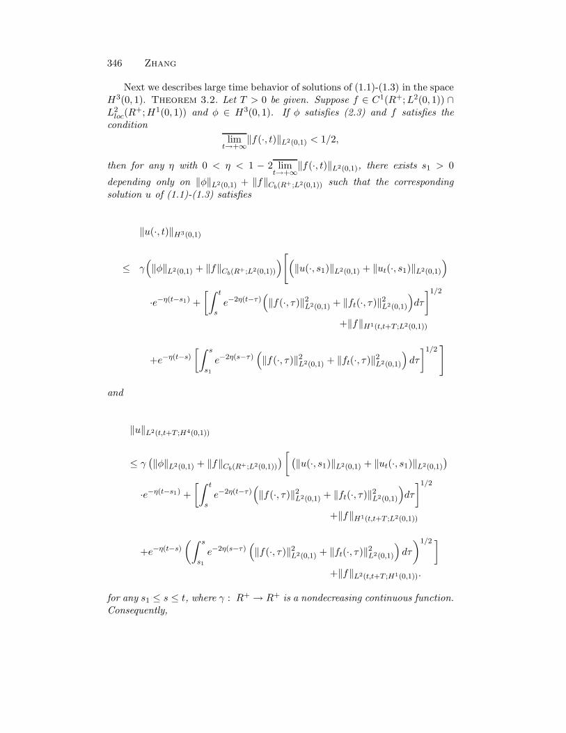
346 Zhang
Next we describes large time behavior of solutions of (1.1)-(1.3) in the spaceH3(0, 1). Theorem 3.2. Let T > 0 be given. Suppose f ∈ C1(R+;L2(0, 1)) ∩L2loc(R
+;H1(0, 1)) and φ ∈ H3(0, 1). If φ satisfies (2.3) and f satisfies thecondition
limt→+∞
‖f(·, t)‖L2(0,1) < 1/2,
then for any η with 0 < η < 1 − 2 limt→+∞
‖f(·, t)‖L2(0,1), there exists s1 > 0
depending only on ‖φ‖L2(0,1) + ‖f‖Cb(R+;L2(0,1)) such that the correspondingsolution u of (1.1)-(1.3) satisfies
‖u(·, t)‖H3(0,1)
≤ γ(‖φ‖L2(0,1) + ‖f‖Cb(R+;L2(0,1))
)[(‖u(·, s1)‖L2(0,1) + ‖ut(·, s1)‖L2(0,1)
)·e−η(t−s1) +
[∫ t
se−2η(t−τ)
(‖f(·, τ)‖2
L2(0,1) + ‖ft(·, τ)‖2L2(0,1)
)dτ
]1/2
+‖f‖H1(t,t+T ;L2(0,1))
+e−η(t−s)[∫ s
s1
e−2η(s−τ)(‖f(·, τ)‖2
L2(0,1) + ‖ft(·, τ)‖2L2(0,1)
)dτ
]1/2]
and
‖u‖L2(t,t+T ;H4(0,1))
≤ γ(‖φ‖L2(0,1) + ‖f‖Cb(R+;L2(0,1))
) [ (‖u(·, s1)‖L2(0,1) + ‖ut(·, s1)‖L2(0,1)
)·e−η(t−s1) +
[∫ t
se−2η(t−τ)
(‖f(·, τ)‖2
L2(0,1) + ‖ft(·, τ)‖2L2(0,1)
)dτ
]1/2
+‖f‖H1(t,t+T ;L2(0,1))
+e−η(t−s)(∫ s
s1
e−2η(s−τ)(‖f(·, τ)‖2
L2(0,1) + ‖ft(·, τ)‖2L2(0,1)
)dτ
)1/2 ]+‖f‖L2(t,t+T ;H1(0,1)).
for any s1 ≤ s ≤ t, where γ : R+ → R+ is a nondecreasing continuous function.Consequently,

Forced Oscillation of the KdV-Burgers Equation 347
(i) if limt→+∞
(‖f(·, t)‖L2(0,1) + ‖ft(·, t)‖L2(0,1) + ‖f‖L2(t,t+T ;H1(0,1))
)= 0, then
limt→+∞
‖u‖Y 3t,t+T
= 0;
(ii) if ‖f(·, t)‖L2(0,1) + ‖ft(·, t)‖L2(0,1) + ‖f‖L2(t,t+T ;H1(0,1)) < Ce−αt, for someα > 0 and any t ≥ 0, then
‖u‖Y 3t,t+T
≤ γ(‖φ‖L2(0,1) + ‖f‖Cb(R+;L2(0,1))
) [(‖u(·, s1)‖L2(0,1) +
+‖ut(·, s1)‖L2(0,1)
)e−η(t−s1) + Cα,ηCe
−minα,ηt]
for any t ≥ s1, where
Cη,α =
√
1|1−ε−α| + 2√
αif α 6= η,
√t− s1 + 2√
αif α = η.
Proof: Let h = ut. Then h solvesht + hx + (uh)x − hxx + hxxxx = ft,
h(x, 0) = φ∗(x, 0)
h(0, t) = 0, h(1, t) = 0, hx(1, t) = 0
withφ∗(x) = f(x, 0) − φ′(x) − φ′′′(x) + φ′′(x) − φ(x)φ′(x).
It holds that
d
dt
∫ 1
0h2(x, t)dx+ 2
∫ 1
0h2x(x, t)dx+ h2
x(0, t)
= 2∫ 1
0ft(x, t)h(x, t)dx + 2
∫ 1
0u(x, t)hx(x, t)h(x, t)dx.
Thus
d
dt‖h(·, t)‖2
L2(0,1) + 2(1 − ε− ‖u(·, t)‖L2(0,1))‖hx(·, t)‖2L2(0,1) ≤
2ε‖f(·, t)‖2
L2(0,1),
from which one obtains
‖h(·, t)‖2L2(0,1) ≤ e−2ηs,t(t−s)‖h(·, s)‖2
L2(0,1) +2ε
∫ t
se−2ηs,t(t−τ)‖ft(·, τ)‖2
L2(0,1)dτ

348 Zhang
and∫ t+T
t‖hx(·, τ)‖2
L2(0,1)dτ ≤ 1εηs,t
∫ t+T
t‖f(·, τ)‖2
L2(0,1)dτ +1
2ηs,t‖h(·, t)‖2
L2(0,1)
for 0 ≤ s ≤ t where
ηs,t = 1 − ε− sups≤τ≤t
‖u(·, τ)‖L2(0,1).
Sincelim
t→+∞‖u(·, t)‖L2(0,1) ≤ 2 lim
t→+∞‖f(·, t)‖L2(0,1) < 1
for given 0 < η < 1 − 2 limt→+∞
‖f(·, t)‖L2(0,1), if let
ε =12(1 − η − 2 lim
t→+∞‖f(·, t)‖L2(0,1)),
then according to Theorem 3.1, there exists s1 > 0 depending only on‖φ‖L2(0,1) + ‖ft‖Cb(R+;L2(0,1)) such that for any s > s1,
infs1≤s≤t<+∞
ηs,t ≥ η.
Thus
‖h(·, t)‖L2(0,1)
≤ e−η(t−s)‖h(·, s)‖L2(0,1) +
√2ε
[∫ t
se−2η(t−τ)‖ft(·, τ)‖2
L2(0,1)dτ
]1/2
for any t ≥ s > s1. In particular,
‖h(·, s)‖L2(0,1)
≤ e−η(s−s1)‖h(·, s1)‖L2(0,1) +
√2ε
[∫ s
s1
e−2η(s−τ)‖ft(·, τ)‖2L2(0,1)dτ
]1/2
for any s > s1 and
‖h(·, t)‖L2(0,1)
≤ e−η(t−s1)‖h(·, s1)‖L2(0,1) +
√2εe−η(t−s1)
[∫ s
s1
e−2η(s−τ)‖ft(·, τ)‖2L2(0,1)dτ
]1/2
+
√2ε
[∫ s
s1
e−2η(s−τ)‖ft(·, τ)‖2L2(0,1)dτ
]1/2
for any s1 < s < t. By Theorem 2.3, there exists a γ = γ(‖(φ, f)‖X0s1
) suchthat
‖h(·, s1)‖L2(0,1) ≤ γ(‖(φ, f)‖X0s1
)‖(φ, f)‖X3s1.

Forced Oscillation of the KdV-Burgers Equation 349
One arrives that
‖ut(·, t)‖L2(0,1) ≤√
2εe−η(t−s)e−η(t−s1)
[∫ s
s1
e−2η(s−τ)‖ft(·, τ)‖2L2(0,1)dτ
]1/2
+
+γ(‖(φ, f )‖X0s1
)‖(φ, f )‖X3s1e−ηt +
√2ε
(∫ s
s1
e−2η(s−τ)‖ft(·, τ)‖2L2(0,1)dτ
)1/2
(3.3)
and
‖ut‖L2t,t+T ;H1(0,1) ≤√
12η
‖ut(·, t)‖L2(0,1) +√
1εη
‖ft‖L2(t,t+T ;L2(0,1))(3.4)
for any s1 ≤ s ≤ t. Recall that
uxxx = f − ut − ux − uux + uxx.(3.5)
There exists a constant C such that
‖uxx(·, t)‖L2(0,1) ≤ C‖uxxx(·, t)‖H−1(0,1)
≤ C(‖f(·, t)‖L2(0,1) + ‖ut(·, t)‖L2(0,1) + ‖u2(·, t)‖L2(0,1) + ‖ux(·, t)‖L2(0,1)
)≤ C
(‖f(·, t)‖L2(0,1) + ‖ut(·, t)‖L2(0,1) + (1 + ‖u(·, t)‖L2(0,1))‖ux(·, t)‖L2(0,1)
).
Thus, for given T > 0,
‖uxx‖L2(t,t+T ;L2(0,1)) ≤ C(‖f‖L2(t,t+T ;L2(0,1)) + ‖ut‖L2(t,t+T ;L2(0,1))
+ supt≤τ≤t+T
(1 + ‖u(·, τ)‖L2(0,1)
)‖ux‖L2(t,t+T ;L2(0,1))
).
It follows from the equation (3.5) again that
‖uxxx‖L2(t,t+T ;L2(0,1)
≤ ‖f − ut − ux‖L2(t,t+T ;L2(0,1)) + ‖uxx − uux‖L2(t,t+T ;L2(0,1))
≤ ‖f − ut − ux‖L2(t,t+T ;L2(0,1)) + supt6τ≤t+T
(1 + ‖u(·, τ)‖L2(0,1)
)‖uxx‖L2(t,t+T ;L2(0,1))
≤ C supt6τ≤t+T
(1 + ‖u(·, τ)‖L2(0,1)
)2(‖f‖L2(t,t+T ;L2(0,1)) + ‖ut‖L2(t,t+T ;L2(0,1))
+‖ux‖L2(t,t+T ;L2(0,1))
).
As u ∈ L2(t, t + T ;H3(0, 1)) and ut ∈ L2(t, t + T ;H1(0, 1))), it yields thatu ∈ C(t, t+ T ;H2(0, 1)) by interpolation and that
supt≤τ≤t+T
‖uxx(·, τ)‖L2(0,1)) ≤ C(‖u‖L2(t,t+T ;H3(0,1)) + ‖ut‖L2(t,t+T ;H1(0,1))
)

350 Zhang
for some constant C independent of t, T and u. Consequently, using (3.5) yieldsthat
‖uxxx(·, t)‖L2(0,1))
≤ ‖f(·, t) − ut(·, t)‖L2(0,1)) + ‖uxx(·, t) − ux(·, t) − u(·, t)ux(·, t)‖L2(0,1))
≤ ‖f(·, t) − ut(·, t)‖L2(0,1)) +(2 + ‖u(·, t)‖L2(0,1))
)‖uxx(·, t)‖L2(0,1))
≤ ‖f(·, t) − ut(·, t)‖L2(0,1)) + C(2 + ‖u(·, t)‖L2(0,1))
)(‖u‖L2(t,t+T ;H3(0,1))
+‖ut‖L2(t,t+T ;H1(0,1))
)≤ ‖f(·, t)‖L2(0,1)) + ‖ut(·, t)‖L2(0,1)) + C sup
t6τ≤t+T
(2 + ‖u(·, τ)‖L2(0,1)
)3
·(‖f‖L2(t,t+T ;L2(0,1)) + ‖ut‖L2(t,t+T ;H1(0,1)) + ‖ux‖L2(t,t+T ;L2(0,1))
)≤ C
(1 + ‖u(·, t)‖L2(0,1) + ‖f‖L2(t,t+T ;L2(0,1))
)3(‖f‖L2(t,t+T ;L2(0,1)) +
+‖ut‖L2(t,t+T ;H1(0,1)) + ‖ux‖L2(t,t+T ;L2(0,1))
)+‖f(·, t)‖L2(0,1)) + ‖ut(·, t)‖L2(0,1))
and
‖uxxxx‖L2(t,t+T ;L2(0,1))
≤ ‖f − ut‖L2(t,t+T ;H1(0,1)) + ‖(ux + uux)x‖L2(t,t+T ;L2(0,1))
+‖uxxx‖L2(t,t+T ;L2(0,1))
≤ ‖f − ut‖L2(t,t+T ;H1(0,1)) + ‖uxx‖L2(t,t+T ;L2(0,1)) + ‖uxxx‖L2(t,t+T ;L2(0,1))
+2‖ux‖L2(t,t+T ;L2(0,1)) supt6τ6t+T
‖uxx(·, τ)‖L2(0,1)
≤ ‖f‖L2(t,t+T ;H1(0,1)) + C(1 + ‖ux‖L2(t,t+T ;L2(0,1))
)(‖u‖L2(t,t+T ;H3(0,1))
+‖ut‖L2(t,t+T ;H1(0,1))
).
Thus there exists a constant Cε,η depending only on η and ε such that for anyt ≥ s1,
‖u(·, t)‖H3(0,1)
≤ Cε,η
(1 + ‖u(·, t)‖L2(0,1) + ‖f‖L2(t,t+T ;L2(0,1)))
)(‖f‖H1(t,t+T ;L2(0,1))
+‖u(·, t)‖L2(0,1) + ‖ut(·, t)‖L2(0,1)
)and
‖u‖L2(t,t+T ;H4(0,1))

Forced Oscillation of the KdV-Burgers Equation 351
≤ ‖f‖L2(t,t+T ;H1(0,1)) + Cε,η
(1 + ‖u(·, t)‖L2(0,1) + ‖f‖L2(t,t+T ;L2(0,1)))
)·(‖f‖H1(t,t+T ;L2(0,1)) + ‖u(·, t)‖L2(0,1) + ‖ut(·, t)‖L2(0,1)
).
Theorem 3.2 follows consequently. The proof is complete.
4 Forced oscillation and its global stability
In this section we assume the forcing f is a time-periodic function of periodω > 0 and study if it generates a time periodic solution for the equation (1.1)with the boundary condition (1.3).
Theorem 4.1. If f ∈ C1b (R
+;L2(0, 1)∩L2loc(R
+,H1(0, 1)) is a time periodicfunction of period ω satisfying
sup0≤t≤ω
‖f(·, t)‖L2(0,1) <14,(4.1)
then the equation (1.1) admits a unique time periodic solution u∗ ∈Cb(R+;H3(0, 1)) of period ω satisfying the boundary conditions (1.3).Proof: For the given forcing f satisfying (4.1), choose φ ∈ H3(0, 1) satisfyingthe compatibility condition (2.3). Let u(x, t) be the corresponding solution ofthe IBVP (1.1)-(1.3). By Theorem 3.2, the set ‖u(·, t)‖H3(0,1)+∞
t=0 is uniformlybounded. Let tk be a sequence with tk → ∞ as k → ∞ such that u(·, tk)converges to a function ψ ∈ H3(0, 1) weakly in H3(0, 1) and strongly in L2(0, 1)as k → ∞. If one takes ψ as an initial data in the IBVP (1.1)-(1.3) with thegiven forcing f , then the corresponding solution, named as u∗(x, t), is a timeperiodic function of period ω. To see this is true, let v(x, t) = u(x, t+ω)−u(x, t).Because of the periodicity of f , v(x, t) solves the following linear problem withthe variable coefficient b(x, t) = u(x, t+ ω) + u(x, t):
vt + vx + (bv)x − vxx + vxxx = 0,
v(x, 0) = φ∗(x),
v(0, t) = 0, v(1, t) = 0, vx(1, t) = 0,
(4.2)
where φ∗(x) = u(x, ω) − u(x, 0). It leads to
d
dt
∫ 1
0v2(x, t)dx + v2
x(0, t) + 2∫ 1
0v2x(x, t)dx = 2
∫ 1
0b(x, t)vx(x, t)v(x, t)dx
ord
dt
∫ 1
0v2(x, t)dx+ 2(1 − ‖b(·)‖L2(0,1))
∫ 1
0v2(x, t)dx ≤ 0
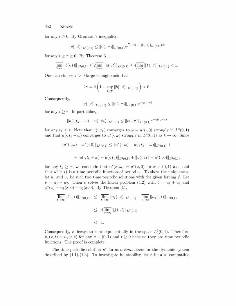
352 Zhang
for any t ≥ 0. By Gronwall’s inequality,
‖v(·, t)‖L2(0,1) ≤ ‖v(·, τ)‖L2(0,1)eR t
τ −2(1−‖b(·,s)‖L2(0,1))ds
for any t ≥ τ ≥ 0. By Theorem 3.1,
limt→∞
‖b(·, t)‖L2(0,1) ≤ 2 limt→∞
‖u(·, t)‖L2(0,1) ≤ 4 limt→∞
‖f(·, t)‖L2(0,1) < 1.
One can choose τ > 0 large enough such that
2γ = 2(
1 − supt≥τ
‖b(·, t)‖L2(0,1)
)> 0.
Consequently,‖v(·, t)‖L2(0,1) ≤ ‖v(·, τ)‖L2(0,1)e
−γ(t−τ)
for any t ≥ τ . In particular,
‖u(·, tk + ω) − u(·, tk)‖L2(0,1) ≤ ‖v(·, τ)‖L2(0,1)e−γ(tk−τ)
for any tk ≥ τ . Note that u(·, tk) converges to ψ = u∗(·, 0) strongly in L2(0, 1)and that u(·, tk + ω) converges to u∗(·, ω) strongly in L2(0, 1) as k → ∞. Since
‖u∗(·, ω) − u∗(·, 0)‖L2(0,1) ≤ ‖u∗(·, ω) − u(·, tk + ω)‖L2(0,1) +
+‖u(·, tk + ω) − u(·, tk)‖L2(0,1) + ‖u(·, tk) − u∗(·, 0)‖L2(0,1)
for any tk ≥ τ , we conclude that u∗(x, ω) = u∗(x, 0) for x ∈ (0, 1) a.e. andthat u∗(x, t) is a time periodic function of period ω. To show the uniqueness,let u1 and u2 be such two time periodic solutions with the given forcing f . Letv = u1 − u2. Then v solves the linear problem (4.2) with b = u1 + u2 andφ∗(x) = u1(x, 0) − u2(x, 0). By Theorem 3.1,
limt→∞
‖b(·, t)‖L2(0,1) ≤ limt→∞
‖u1(·, t)‖L2(0,1) + limt→∞
‖u2(·, t)‖L2(0,1)
≤ 4 limt→∞
‖f(·, t)‖L2(0,1)
< 1.
Consequently, v decays to zero exponentially in the space L2(0, 1). Thereforeu1(x, t) ≡ u2(x, t) for any x ∈ (0, 1) and t ≥ 0 because they are time periodicfunctions. The proof is complete.
The time periodic solution u∗ forms a limit circle for the dynamic systemdescribed by (1.1)-(1.3). To investigate its stability, let φ be a s−compatible

Forced Oscillation of the KdV-Burgers Equation 353
function in the phase space Hs(0, 1) and u be the corresponding solution of theIBVP (1.1)-(1.3). If let w = u− u∗, then w solves the equation
wt + wx + wwx + (u∗w)x −wxx + wxxx = 0
and satisfies the initial condition w(x, 0) = φ − u∗(x, 0) and the homogeneousboundary condition (1.3). This leads us to considering the large time behaviorof the following initial-boundary-value problem
ut + ux + uux + (vu)x + uxxx − uxx = 0,
u(x, 0) = φ(x),
u(0, t) = 0, u(1, t) = 0, ux(1, t) = 0
(4.3)
for x ∈ (0, 1) and t ≥ 0 where v ≡ v(x, t) is a given functionwith v ∈ C(R+;H3(0, 1)) ∩ L2
loc(R+;H4(0, 1)) and vt ∈ C(R+;L2(0, 1)) ∩
L2loc(R
+;H1(0, 1)). By the same arguments used in the section 2 one can showthat (4.3) is globally well-posed in the space Hj(0, 1) for j = 0, 3. As for itslarge time behavior, we have the following result.
Proposition 4.2. Let T > 0 and j = 0 or 3 be given. There exist constantsη1 ∈ (0, 1) and η2 > 0 such that if
limt→∞
‖v‖Y 0t,t+T
< η1,(4.4)
then for φ ∈ Hj(0, 1) with φ satisfying (2.3) if j = 3, the unique solution u of(4.3) satisfies
‖u(·, t)‖Hj (0,1) ≤ γ(‖φ‖L2(0,1)
)e−η2t‖φ‖Hj(0,1)(4.5)
for any t ≥ 0, where γ : R+ → R+ is a nondecreasing continuous functiondepending on j, T and v.
The following stability result for the forced oscillation u∗(x, t) then follows.Theorem 4.3. There exists an η ∈ (0, 1) such that if f ∈ C1
b (R+;L2(0, 1) ∩
L2loc(R
+,H1(0, 1)) is a time periodic function of period ω satisfying
sup0≤t≤ω
‖f(·, t)‖L2(0,1) < η,
then the equation (1.1) admits a unique time periodic solution u∗ ∈Cb(R+;H3(0, 1)) of period ω satisfying the boundary conditions (1.3). More-over, for given j = 0, 3, there exists a δ > 0 such that for any compatibleφ ∈ Hj(0, 1) with φ satisfying (2.3) if j = 3, the corresponding solution u of(1.1)-(1.3) satisfies
‖u(·, t) − u∗(·, t)‖Hj (0,1) ≤ Ce−δt

354 Zhang
for any t ≥ 0. In other words, the set u∗(·, t), 0 ≤ t ≤ ω, as a limit circle,forms an inertial manifold in the space Hj(0, 1) for the dynamic system (1.1)-(1.3).
Indeed, for given compatible φ ∈ Hj(0, 1), let u(x, t) be the correspondingsolution. Then w(x, t) = u(x, t) − u∗((x, t) solves the system (4.3) withv(x, t) = u∗(x, t) and φ∗(x) = φ(x) − u∗(x, 0). By Theorem 3.1, one maychoose η small enough such that
limt→∞
‖u∗‖Y 0t,t+T
< η1,
where η1 is as given in Proposition 4.1. If Proposition 4.2 holds, then thereexist τ > 0 and δ > 0 such that
‖w(·, t)‖Hs(0,1) ≤ γ(‖w(·, τ)‖L2(0,1))‖w(·, τ)‖Hj (0,1)e−δ(t−τ)
for any t ≥ τ , which yields Theorem 4.3. Thus it remains to prove Proposition4.2.Proof of Proposition 4.2: For the solution u of (4.3) it holds that
d
dt
∫ 1
0u2(x, t)dx+ u2
x(0, t) + 2∫ 1
0u2x(x, t)dx = 2
∫ 1
0ux(x, t)u(x, t)v(x, t)dx
for any t ≥ 0, which implies that
d
dt
∫ 1
0u2(x, t)dx+ 2(1 − ‖v(·, t)‖L2(0,1))
∫ 1
0u2x(x, t)dx ≤ 0
for any t ≥ 0. By the assumption (4.4), there exists s > 0 such that
sups≤t<∞
(1 − ‖v(·, t)‖L2(0,1)) = η > 0.
Thus ∫ 1
0u2(x, t)dx ≤ e−2η(t−s)‖u(·, s)‖2
(0,1)
and ∫ t+T
tu2x(x, τ)dxdτ ≤ 1
η
∫ 1
0u2(x, t)dx
for any t ≥ s. The estimate (4.5) with j = 0 follows consequently.
To see Proposition 4.2 holds for j = 3, let u be the solution of (4.3) andh = ut. Then h solves
ht + ((v + u)h)x + hxxx − hxx = −(uvt)x,
h(x, 0) = φ∗(x),
h(0, t) = 0, h(1, t) = 0, hx(1, t) = 0

Forced Oscillation of the KdV-Burgers Equation 355
for x ∈ (0, 1) and t ≥ 0 where
φ∗(x) = −φ′′′(x) − v(x, 0)φ′(x) − vx(x, 0)φ(x) + φ′′(x).
Its integral form is given by
h(t) = W (t−s)h(s)−∫ t
sW (t−τ)(h(v+u))x(·, τ)dτ−
∫ t
sW (t−τ)(uvt)x(·, τ)dτ
for any 0 ≤ s ≤ t < +∞. For a given T > 0, let Q = W (T + s), qk = h(kT + s),
fk = −∫ (k+1)T+s
kT+sW ((k + 1)T + s− τ)(uvt)x(·, τ)dτ
and
g(qk) = −∫ (k+1)T+s
kT+sW ((k + 1)T + s− τ)((u+ v)h)x(·, τ)dτ
for k = 0, 1, 2, · · · . We have then
qk+1 = Qqk + g(qk) + fk, k = 0, 1, 2, · · · .
Note that there exists a constant C1 depending only on T , v and ‖φ‖L2(0,1) suchthat
‖fk‖L2(0,1) ≤ 2√T‖vt‖Y 0
kT+s,(k+1)T+s‖u‖Y 0
kT+s,(k+1)T+s
and‖g(qk)‖L2(0,1) ≤ CTak‖qk‖L2(0,1),
where ak = ‖u+ v‖Y 0kT+s,(k+1)T+s
. Since ‖Q‖ < 1 and
limt→∞
‖u+ v‖Y 0kT+s,(k+1)T+s
≤ η1
by the estimate (4.5) with j = 0 we have just proved, one can choose η1 and ssuch that, for any k ≥ 0,
‖Q‖ + CTak = α < 1
and‖fk‖ ≤ C2‖u(·, s)‖L2(0,1)β
k,
where 0 ≤ β < 1 and the constant C2 depends only on ‖vt‖Cb(R+;L2(0,1)) and T .As a result, for such chosen η1 and s,
‖qk+1‖L2(0,1) ≤ α‖qk‖L2(0,1) + C2βk

356 Zhang
for any k ≥ 0, which leads to
‖qk+1‖L2(0,1) ≤ αk‖q0‖L2(0,1) + C2‖u(·, s)‖L2(0,1)
k∑j=0
αjβk−j
or
‖qk+1‖L2(0,1) ≤ αk‖q0‖L2(0,1) + C2kηk‖u(·, s)‖L2(0,1)
= αk‖ut(·, s)‖L2(0,1) + C2kηk‖u(·, s)‖L2(0,1)
for any k ≥ 0 where η = minα, β.Hence there exists a η2 > 0 such that
‖h‖Y 0t,t+T
= ‖ut‖Y 0t,t+T
≤ γ1
(‖φ‖L2(0,1)
)‖φ‖H3(0,1)e
−η2t
for any t ≥ 0 where γ1 : R+ → R+ is a nondecreasing function depending onlyon v and T. It follows from the equation
uxxx = −uux − ux + uxx − ut − (vu)x
by the same argument as that used in the proof of Theorem 3.2 that
‖u‖Y 3t,T+t
≤ γ(‖φ‖L2(0,1)
)e−η2t‖φ‖H3(0,1)
for any t ≥ 0. The proof is complete.
References
[1] C. J. Amick, J. L. Bona and M. E. Schonbek, Decay of solutions of some nonlinearwave equations. J. Differential Equations 81 (1989), 1–49.
[2] J. L. Bona and L. Luo, Decay of solutions to nonlinear, dispersive wave equations,Diff. & Integral Equ. 6 (1993), 961–980.
[3] J. L. Bona, V. A. Dougalis, An initial and boundary value problem for a modelequation for propagation of long waves, J. Math. Anal. Appl. 75 (1980), 503–522.
[4] J. L. Bona and L. Luo, Initial-boundary-value problems for model equations forthe propagation of long waves, Evolution equations (Baton Rouge, LA, 1992), 63,65–94, Lecture Notes in Pure and Appl. Math., 168, Dekker, New York, 1995.
[5] J. Bourgain, Construction of periodic solutions of nonlinear wave equations inhigher dimension, Geom. Funct. Anal., 5 (1995), 105 – 140.
[6] H. Brezis, Periodic solutions of nonlinear vibrating strings and duality principles,Bull. Amer. Math. Soc., 8 (1983), 409 – 425.
[7] P. Constantin, C. Foiacs, B. Nicolaenko and R. Temam, Integral manifoldsand inertial manifolds for dissipative partial differential equations, AppliedMathematical Sciences, 70 (1989), Springer-Verlag, New York-Berlin

Forced Oscillation of the KdV-Burgers Equation 357
[8] W. Craig and C. E. Wayne, Newton’s method and periodic solutions of nonlinearwave equations, Comm. Pure Appl. Math., 46 (1993), 1409–1498.
[9] J. B. Keller and L. Ting, Periodic vibrations of systems governed by nonlinearpartial differential equations, Comm. Pure and Appl. Math. (1966), 371 – 420.
[10] J. U. Kim, Forced vibration of an aero-elastic plate, J. Math. Anal. Appl.113 (1986), 454–467.
[11] R. M. Miura, The Korteweg-de Vries equation: A survey of results, SIAM review18 (1976), 412 – 459.
[12] P. H. Rabinowitz, Periodic solutions of nonlinear hyperbolic differential equations,Comm. Pure Appl. Math. 20 (1967), 145 – 205.
[13] P. H. Rabinowitz, Free vibrations for a semi-linear wave equation, Comm. PureAppl. Math. 31 (1978), 31 – 68.
[14] D. L. Russell and B.-Y. Zhang, Controllability and stabilizability of the third-order linear dispersion equation on a periodic domain, SIAM J. Contr. Optim.31 (1993), 659–676.
[15] D. L. Russell and B.-Y. Zhang, Exact controllability and stabilizability of theKorteweg-de Vries equation, Trans. Amer. Math. Soc. 348 (1996), 3643–3672
[16] D. L. Russell and B.-Y. Zhang, Smoothing and decay properties of solutions ofthe Korteweg-de Vries equation on a periodic domain with point dissipation, J.Math. Anal. Appl. 190 (1995), 449–488.
[17] O. Vejvoda, partial differential equations: time-periodic solutions, Mrtinus NijhoffPublishers, 1982.
[18] C. E. Wayne, Periodic solutions of nonlinear partial differential equations, NoticesAmer. Math. Soc. 44 (1997), 895–902.
[19] C. E. Wayne, Periodic and quasi-periodic solutions of nonlinear wave equationsvia KAM theory, Comm. Math. Phys. 127 (1990), 479 – 528.
[20] B.-Y. Zhang, Analyticity of solutions for the generalized Korteweg-de Vriesequation with respect to their initial datum, SIAM J. Math. Anal. 26 (1995),1488–1513.


![An Online Parameter Estimation Tool · # Nonlinear state function $ Nonlinear observer function Tailplane trim angle ... identification and hence parameter estimation effort [9,10]](https://img.dokumen.tips/doc/110x75/5e86752d23474e477705949f/an-online-parameter-estimation-tool-nonlinear-state-function-nonlinear-observer.jpg)