Distributed parameter model simulation tool

for PEM fuel cells

Maria Sarmiento-Carnevalia,1, Maria Serraa, Carles Batlleb

aInstitut de Robotica i Informatica Industrial (CSIC-UPC), C/ Llorens i Artigas 4-6,08028 Barcelona

bDepartament de Matematica Aplicada IV & IOC, Universitat Politecnica de Catalunya,EPSEVG, Av. V. Balaguer s/n, 08800 Vilanova i la Geltru

Abstract

In this work, a simulation tool for proton exchange membrane fuel cells

(PEMFC) has been developed, based on a distributed parameter model.

The tool is designed to perform studies of time and space variations in the

direction of the gas channels. Results for steady-state and dynamic simula-

tions for a single cell of one channel are presented and analyzed. Considered

variables are concentrations of reactants, pressures, temperatures, humidifi-

cation, membrane water content, current, among others that have significant

effects on the performance and durability of PEMFC.

Keywords: PEMFC, distributed parameter modeling, dynamic simulation

1. Introduction

The proton exchange membrane fuel cells (PEMFC) technology has been

incorporated to a wide range of portable, stationary and automotive appli-

cations in recent years [1]. However, despite current developments, PEMFC

1Corresponding author. Tel.: +34 (93) 401 58 05; fax: +34 (93) 401 57 50. E-mailaddress: m.sarmiento@iri.upc.edu (M.L. Sarmiento-Carnevali).

Preprint submitted to International Journal of Hydrogen Energy April 5, 2013

are still not accepted as a practical power generator. The key challenge is to

reduce the cost and achieve a high performance and long life of the cells.

Along-the-channel variations of important variables such as concentra-

tions of hydrogen, oxygen and water, as well as temperature, have significant

effects on the performance and durability of PEMFC. All these variables ex-

hibit spatial dependence in the direction of the channels of the anode and

cathode and, therefore, it is necessary to introduce partial differential equa-

tions (PDE) to accurately model such variations.

Distributed parameter first principles modeling allows, indeed, the de-

tailed study of the fundamental phenomena that occur within a PEMFC.

Bernardi and Verbrugge [2] and Springer et al. [3] developed pioneering dis-

tributed parameter models. These models, both one-dimensional, analyzed

species transport, water addition and removal, cathode flooding and the effect

of gas humidification. Later, Rowe and Li [4] developed a one-dimensional,

non-isothermal model of a PEM fuel cell, incorporating water and temper-

ature distribution to investigate the operating conditions effects on the cell

performance, thermal response and water management.

Methekar [5] developed a two-dimensional, along-the-channel, distributed

parameter model to perform dynamic analysis and design linear control

strategies for PEMFC. A detailed two-dimensional simulation model was

presented by Mangold et al. [6] for control purposes. Um et al. [7] developed

a 2D model to simulate proton exchange membrane fuel cells. The model

accounts simultaneously for electrochemical kinetics, current distribution,

hydrodynamics, and multicomponent transport. A single set of conservation

equations valid for flow channels, gas diffusion electrodes, catalyst layers,

2

and the membrane region are presented. Kulikovsky [8] published a semi-

analytical model of PEMFC, which takes into account oxygen and water

transport across the cell and along the channel. The two-dimensional mod-

els can be divided into two categories. One group of models describes the

plane perpendicular to the flow channels, while the other group of models

describes the direction across the fuel cell and the direction along the flow

channel. Each group has its advantages and drawbacks. In the first group of

models, the effect of flow channel dimension and configuration can be stud-

ied, however, changes in the temperature and reactants fraction cannot be

accounted for. The second group of models can predict the temperature and

concentration profiles along the direction of the flow channel, but cannot

simulate the effect of flow channel and rib size.

Three-dimensional models have been developed by various research groups

[3, 9]. Schumacher et al. [10] presented a 2D + 1D to take the in-plane

and the through-plane dimensions of fuel cells into account. The anode and

cathode are included as 2D domains, and a nonlinear 1D model represents

the membrane electrode assembly (MEA). Tao [11] developed an important

three-dimensional, two-phase, non-isothermal unit cell model in order to per-

form parameter sensitivity examination. Um and Wang [12] developed a com-

putational fuel cell dynamics (CFCD) model to study three-dimensional (3D)

interactions between mass transport and electrochemical kinetics in PEMFC.

In addition to different geometrical assumptions, important multiscale mod-

eling approaches have been published [13, 14, 15]. Multiscale models allow

the study of system behavior at different levels (from smaller to larger scales).

On each level, particular approaches are used for description of the system.

3

Following levels are usually distinguished: quantum mechanical models (in-

formation about electrons is included), level of molecular dynamics models

(information about individual atoms is included), mesoscale or nano level

(information about groups of atoms and molecules is included), level of con-

tinuum models, level of device models, among others.

Moreover, there are various simulation tools for PEMFC [16], but very

few are flexible enough to manipulate the underlying model equations. This

work is focused on the development of a simulation tool for two intended

purposes: (1) the analysis of variables with important spatial variations along

the channel, and (2) the application of model order reduction techniques to

design distributed parameter model-based controllers, aimed at the control

of these spatial variations [17].

In this work, the implemented tool is based on a distributed parameter

model (1 + 1D) to be used in model-based controllers. This type of 2D

models facilitates the detailed study of along-the-channel spatial variations

of important variables regarding performance and durability of PEMFC, as

well as a simplified analysis of variables in the direction across the MEA

(important for water transport studies), by approximating spatial gradients.

Therefore, the emphasis on channel direction profiles makes the model suit-

able for control design that takes into account spatial profiles, and simple

enough (not being a 1D model) to apply model order reduction techniques

that are very complex. These features make the model an appropriate choice

over the wide range of geometrical assumptions, such as 2D, 2D+1D, 3D

(previously mentioned and referenced).

The paper is organized as follows. Section 2 shows the structure of the

4

modeled system. Section 3 describes the model equations. Section 4 covers

the tasks of simulation tool development (discretization and implementation).

Section 5 presents simulation results and Section 6 concludes on the work

developed.

2. Description of the system

This work considers a single cell of one channel (Fig. 1) that includes all

the functional parts of the PEMFC: bipolar plates (BP), gas channels (GC),

gas diffusion layers (GDL), catalyst electrode layers (CL), a proton exchange

membrane and a cooling system. This simple model suits the detailed anal-

ysis of spatial variations. The case study selected in the work is a 0.4 m

along-the-channel single cell (area 0.4 x 10-3 m) with Nafion 117 membrane.

The parameters of the membrane are taken from [18, 19].

3. Distributed parameter model

The model equations are based on the work by Mangold et al. [6]. This is

not only a recent model, but it is also one of the most detailed set of PEMFC

equations in the open literature. The model is 1+1D with approximation of

gradients by a fixed number of points in y-direction and partial differential

equations (PDE) along the channel (z-direction) (Fig. 1).

Physical phenomena occurring within the gas channels is represented by

the solution of conservative equations for mass, momentum and energy. The

principle of mass conservation is used to model reactant concentrations. A

pressure drop relation, derived from simplified Navier-Stokes equations, al-

lows the calculation of the flow velocity. The ideal gas law is used to calculate

5

Figure 1: Structure of the fuel cell considered in this work

flow pressure. An energy balance is used to determine the flow temperature.

Stefan-Maxwell diffusion equations for a multicomponent gas are used to

define the mole fraction gradient in the gas diffusion layers (GDL). The reac-

tion rates are modeled by Butler-Volmer equations and Faraday’s law. Mem-

brane behavior is described by the calculation of membrane water content,

water concentration, drag coefficient, net water flux and protonic conductiv-

ity. The gas diffusion layers (GDL), catalyst layers (CL) and membrane are

considered to be at the same temperature level. These PEMFC components

form the solid part (SP).

Liquid water formation is not considered. The model validity is restricted

to one-phase conditions, where condensation in gas channel and gas diffusion

layers is negligible. Considering liquid water formation is a future objective

but, in this moment, using the simulation tool for control purposes by means

6

of model order reduction techniques is a priority.

An energy balance for the solid part, similar to the energy balances of the

gas channels (GC), is used to calculate the solid part temperature. Current

transport is described by governing equations for conservation of charge and

the cell potential is calculated by the polarization curve equation. In this

relation, activation polarization losses, ohmic losses and concentration losses

are considered. The combination of these laws results in a set of PDE and

algebraic constraints.

In this work, important effort on presenting membrane model details and

calculations has been made. In addition, the entire spatial discretization pro-

cess of equations describing PEMFC phenomena is presented. Moreover, a

widely used software (Matlab R©) was selected to develop the simulation tool.

Finally, interesting and different results are presented: along-the-channel be-

havior and time evolution of variables at specific channel points. Actually,

there is special emphasis on spatial and temporal variance analysis, given its

importance for performance and durability of PEMFC.

4. Model implementation

The set of PDE and algebraic constraints was discretized spatially along

the channel using finite differences [20]. As a result, a set of differential alge-

braic equations (DAE) was obtained [21]. This new set of model equations

was implemented and numerically solved in Matlab R©, using a DAE solver.

4.1. Model discretization

Partial differential equations and algebraic constraints have been dis-

cretized by finite differences into MZ points (uniformly distributed) along

7

z-direction, starting from z = 0 m (first point) until z = 0.4 m (channel

length). Along y-direction, only a few points are considered, depending on

the submodel of interest. For variables such as different temperatures lev-

els, no y-direction variation is considered (gas channels temperatures, for

instance). However, for variables such as water fluxes or molar fractions, dif-

ferent points along y-direction are studied (middle point of channel, middle

point of membrane, membrane boundary to anode side, membrane boundary

to cathode side, among others). In the following sections, all the discretized

equations and their purpose within the model are presented (k is an index

that denotes mesh points).

4.1.1. Gas channels submodel

The gas channel equations allow the calculation of concentration of gases,

flow velocities, flow pressure and temperature in the gas channels.

• Mass balances equations

The general equation for mass conservation is discretized as follows:

dcji,kdt

= −vj

kcji,k − v

jk−1c

ji,k−1

∆z−nj

i,k

δj(1)

From these equations, the values of the concentrations cji,k at each mesh

point, but the first, are determined. The boundary condition remains an

algebraic equation as follows:

vj0c

ji,0|0,t = nj

i,in (2)

8

This algebraic equation is used to calculate concentrations at the begin-

ning of the gas channels.

The superscript j is used to denote anode side (A) or cathode side(C).

The subscript i indicates the species index. On anode side, it can be either

H2 or H2O. The water component might be present in the case of hydrogen

humidification [20]. On cathode side, i can be either O2, or N2 or H2O, δj is

gas channel thickness in y-direction (Fig. 1), nji denote molar flow densities

between gas channels and gas diffusion layers, nji,in denote inlet molar flow

densities (inlet flow divided by cross-sectional area of the gas channels [6]).

• Flow velocity equations

Normally, velocity vectors for flow dynamics are determined by the con-

servation of momentum equations, the so-called Navier-Stokes equations [22].

Considering a set of assumptions, such as neglecting the acceleration terms,

the Navier-Stokes equation can be simplified into a pressure drop relation

similar to Darcy’s law [22]. Calculation of flow velocities for both anode gas

channel and cathode gas channel, using forward differencing is:

vjk = −Kj p

jk+1 − p

jk

∆z(3)

Considering boundary condition (MZ is the number of mesh points):

vjMZ = −Kj p

amb − pjMZ−1

∆z(4)

• Flow pressure equations

Ideal gas law is used to calculate flow pressure in the gas channels, and

this equation also relates pressure with total gas concentration. This is:

9

pjk = RT j

k

∑i

cji,k (5)

• Energy balance equations

Accumulation of energy in the gas channels is:

d (ρu)j

dt= − 1

∆z

(∑i

vjcji,khi,k

(T j

k

))(6)

+1

∆z

(∑i

vjcji,k−1hi,k−1

(T j

k−1

))

+λj Tjk+1 − 2T j

k + T jk−1

∆z2

+α1

δj

(T S

k − Tjk

)−∑

i

nji,k

δjhi,k

(T j,k

)where energy changes are given by the terms on the right hand side of (6).

The first term describes energy transport in the z-direction due to convective

flow. The second term represents heat conduction according to Fourier’s

law [23]. The third term is heat transfer between solid fuel cell parts at

temperature T S and gas channels. The last term describes another type

of convective flow from gas channels to the MEA. This is also an enthalpy

transport.

The boundary equations, using backward differencing are:

∑i

nji,inhi

(T j

in

)=∑

i

vj0c

ji,0hi

(T j)|0,t − λj T

j1 − T

j0

∆z|0,t (7)

10

λj TjMZ − T

jMZ−1

∆z|Lz ,t = 0 (8)

• Temperature equations

In order to calculate temperature in the gas channels, a thermodynamic

equation of state is used:

(ρu)jk + pj

k =∑

i

cj,ki hi,k

(T j

k

)(9)

4.1.2. Gas diffusion layers equations

The purpose of the gas diffusion layers (GDL) model is to introduce a

mass transport limitation between gas channels and catalyst layers. The

Stefan-Maxwell diffusion equations for a multicomponent species [2] are used

to define the gradient in mole fraction of the components. These set of

equations is used to calculate mole fractions ξCAH2,k and ξCC

O2,k in the catalyst

layers (kd index is used for mesh points in this case, so there is no confusion

with the k index for species in the original equation):

−5 ξji,kd =

∑k

ξjk,kdn

ji,kd − ξ

ji,kdn

jk,kd

cjDeffi,k

(10)

The gradient of mole fraction 5ξji is:

5ξji,k =

ξCji,k − ξ

ji,k

δGj(11)

The composition inside the GDL 5ξji is:

ξji =

1

2

(ξCji,k − ξ

ji,k

)(12)

11

Finally, the total gas concentration in the GDL follows from:

cjk =pj

k

RT Sk

(13)

4.1.3. Catalyst layers equations

The catalyst layers equations are used to determine the values of the mass

fluxes at each mesh point.

• Mass fluxes through diffusion layers

Due to model assumptions, hydrogen mass flow from the anode gas chan-

nel to catalyst layer is identical to the amount of hydrogen consumed in the

anodic reaction H2 → 2H+ + 2e−:

nAH2,k = rA

k (14)

where rA is the rate of the anodic reaction.

The water flow from the anode gas channel to the GDL is passed on to

the membrane:

nAH2O,k = nAM

H2O,k (15)

The oxygen transported from the cathode gas channel is completely con-

sumed in the cathodic reaction O2 + 4e− + 4H+ → 2H2O. This is:

nCO2,k =

1

2rCk (16)

Nitrogen flow vanishes , since nitrogen is not a reactant and cannot per-

meate through the membrane:

12

nCN2,k = 0 (17)

Water flow from the cathode is given by the cathode catalyst layer water

mass balance:

nCH2O,k = nCM

H2O,k −1

2rCk (18)

• Electrochemistry reactions kinetic rates equations

The reaction rates are modeled by Butler-Volmer equation, which are a

current density-potential relations and Faraday’s law [20], which states that

current density is proportional to the charge transferred and the consumption

of reactant per unit area. For anode reaction, this is [19]:

rA = fV iA0

2F

{exp

(2F

RT Sk

(∆ΦA

k −∆ΦAref

)) ξCAH2,kp

Ak

pH2,ref

− 1

}(19)

rC = fV iC0

2Fexp

(∆G0

R

(1

T Sk

− 1

Tref

))ξCCO2,kp

Ck

pO2,ref

(20)

x exp

(α2F

RT Sk

(∆ΦC

k −∆ΦCref

))

where ΦAM and ΦCM are potentials of the membrane on the anode side and

on the cathode side.

4.1.4. Proton exchange membrane (PEM) equations

The membrane which separates the anode from the cathode must serve

several functions. It should efficiently conduct protons, while preventing

13

electrons and reactant gasses from crossing, and close the electrical circuit

internally by transporting protons from the anode to the cathode. The elec-

trical conductivity of the membrane, strongly depends on membrane hu-

midity. To model this property the simulation model of [18] has been used

(j = AM,CM).

• Water concentration equation

Assuming water is only transported along the y-coordinate, perpendicu-

lar to gas flow, the water concentration is derived from the following mass

balance:

dcMH2O

dt=

1

δM

(nAM

H2O,k + nCMH2O,k

)(21)

• Water content

The protonic conductivity of a polymer membrane is strongly dependent

on membrane structure and its water content. The water content Λ in mem-

brane is usually expressed as grams of water per gram of polymer dry weight,

or as number of water molecules per sulfonic acid groups present in the poly-

mer, Λ = N(H2O)/N(SO3H). In this case, Λ is defined as the ratio between

moles of water in the membrane and moles of polymer in the membrane.

Water content Λ is related to water concentration cMH2O by the following re-

lation:

cMH2O,k = ΛkρMk (Λk)XM

k (Λk) (22)

Membrane density and ion exchange capacity are, respectively:

14

ρM = ρ0ρdry1 + ΛkMoXdry

ρ0 + ΛkMoXdryρdry

(23)

XM =Xdry

(1 + ΛkMoXdry)(24)

The mole fractions of water protons and protons in the membrane are

calculated from:

ξH2O (Λk) =Λk

Λk + 2(25)

ξH+ (Λk) =1

Λk + 2(26)

• Water fluxes through the membrane equations

The water flows through the membrane are assumed to be driven by gra-

dients of chemical potentials of water and protons. This is an electrochemi-

cal method developed by [20], based on electrochemical potential that arises

across a membrane sample exposed at each side to different water activities.

njH2O,k = −tW (Λk)κ (Λk)

F 25 µj

H+,k −DW (Λk) cMH2O,k

RT Sk

5 µjH2O,k (27)

Water is dragged from the anode to the cathode by protons moving

through the membrane. This is called electroosmotic drag. The flux of

water due to electroosmotic drag is given by the left term of the right hand

side of 27. Moreover, water generation and electroosmotic drag create a large

15

concentration gradient across the membrane. Because of this gradient, water

diffuses back from the cathode to the anode. The other term of the right

hand side reflects back-diffusion of water. The electroosmotic drag coefficient

tW relation and the water diffusion coefficient DW relation are taken from

[18].

The gradients of chemical potential are calculated from:

5µjH2O,k =

RT S, k

ξH2O,k (Λ)5 ξj

H2O,k (28)

5µjH+,k =

RT S

ξH+,k (Λk)5 ξj

H+,k + F 5 Φ (29)

5ξjH2O

=ξH2O (Λ)− ξH2O (Λj)

δM/2(30)

As it was done in the GDLs model, the gradients are approximated by

simple difference formulas:

5ξjH+ =

ξH+ (Λ)− ξH+ (Λj)

δM/2(31)

5Φ =ΦCM − ΦAM

δM(32)

Water contents at membrane boundaries to the anode side ΛAM and cath-

ode side ΛCM depend on the relative humidity in the catalyst layers. As

shown in the next chapter, calculation is given by sorption isotherms taken

from [18].

• Electrical current density equations

16

Electrical current through the membrane is related to proton flow by:

iM = FnH+,k (33)

• Proton flux equations

Similar to the water flux, the proton flux is driven by gradients of elec-

trochemical potentials:

nH+,k = −κ (Λk)

F 25 µH+ −

tW (Λk)κ (Λk)

F 25 µH2O (34)

Considering there is no accumulation of protons in the membrane, is

calculated as follows. This is a set of equations added to the [6] simulation

model.

5µH2O,k =RT S

k

ξH2O,k (Λk)5 ξH2O (35)

5µH+,k =RT S

ξH+,k (Λk)5 ξH+ + F 5 Φ (36)

5ξH2O,k =ξH2O,k

(ΛCM

k

)− ξH2O,k

(ΛAM

k

)δM

(37)

5ξjH+,k =

ξH+

(ΛCM

k

)− ξH+,k

(ΛAM

)δM

(38)

5Φk =ΦCMk − ΦAMk

δM(39)

17

4.1.5. Solid part energy balance

Similar to the gas channels energy balance, the energy balance for the

solid part (SP) is:

δs∂ (ρe)j

∂t=∑i,j

njihi

(T j

k

)+∑

j=A,C

α1

(T j

k − TSk

)(40)

+α2

(T cool

k − T Sk

)+

λsδs Tj

∆z2−(ΦC

k − ΦAk

)iMk

where energy changes are given by the terms on the right hand side of 40.

This is mass exchange between gas channels and SP, heat exchange between

gas channels and SP, heat exchange between coolant and SP, Fourier heat

conduction and electrical work.

The total energy relation is defined as internal energy (enthalpies of the

different parts of the MEA) and electrical energy in the double layers. This

is:

δs (ρek) = δs (ρuk) + CAδACk

∆ΦA2

k

2+ CCδCC

k

∆ΦC2

k

2

= δs(ρh) (T S)

+ CAδAC ∆ΦA2

2+ CCδCC ∆ΦC2

2(41)

where:

18

δs(ρh) (T S

k

)=(δS − δM

)(ρh)S

k

(T S

k

)+

δM (ρhk)M (T Sk

)+ δMρM

H2O,khH2O,k

(T S

k

)(42)

4.1.6. Conservation of charge equations

Current transport is described by a governing equations for conservation

of charge [20]. In this model, it is assumed that charge is transported in the

direction of the z-coordinate, and through the membrane, in the direction of

the y-coordinate. Charge balances are:

CAδAC d∆ΦAk

dt= iMk − 2FrA

k (43)

CCδCC d∆ΦC

dt= iMk − 2FrC

k (44)

4.1.7. Cell current

The total cell current is given by [20]:

I = Lx

(Lz∑k

iMk

)∆z (45)

4.1.8. Cell potential

U (t) = ∆ΦC (z, t)−∆ΦM (z, t)−∆ΦA (z, t) (46)

In this relation activation polarization losses (energy activation barrier)

and ohmic losses (potential drop in the membrane) are considered.

19

4.2. Numerical implementation

The simulation model consists of six submodels that are coupled by inter-

nal variables. The GC module models reactant concentrations, flow velocity,

pressure and temperature in the gas channels. The GDL module studies

diffusion in a multicomponent mix of species. The electrochemical reactions

and mass fluxes are modeled in the CL submodel. The membrane module

consists of a detailed protonic exchange membrane model [8].

The solid part module consists of an energy balance to determine the

solid part temperature. Finally, cell current and voltage are determined in

the charge balances module. The inputs are inlet flows for anode side and

cathode side, inlet flows temperatures, cooling temperature and cell voltage.

The main output is cell current, but it is possible to have cell current as an

input instead of cell voltage. This depends on the operation mode desired.

The set of model equations (DAE) was implemented and numerically

solved with Matlab R© using the ODE15s solver (DAE solver). Performing

simulations is very simple. There are two main m-files, the model equations

file and the model simulation file. The former is a function file that contains

the whole set of differential algebraic equations (all submodels equations cou-

pled by each module variables), the latter generates the numerical solutions,

by calling the solver, and the graphics of variables dynamics (set of surfaces).

There are more options to generate specific graphics such as along-the-

channel steady-state results, along-time results and specific outputs such as

oxygen and hydrogen stoichiometry, relative humidity, and others, but these

are optional m-files. It is also possible to use each submodule separately

(separate m-files), by considering coupling variables as constant profiles. This

20

option is suitable when studying the behavior of specific cell components.

The tool is intended to analyze along-the-channel behavior through time,

and design model-based controllers that consider spatial variations. For this

purpose the model has to be reduced by means of complex model order re-

duction techniques. However, as ongoing work, the simulation tool is being

migrated to Simulink, to precisely make it suitable to a larger system sim-

ulation and test conventional controllers such as FeedForward or PID. This

means using the tool as a lumped parameter model, and still being able to

study spatial profiles of PEMFC variables.

5. Simulation results

In order to show the possibilities of the tool, the results of simulations for

different variables are shown. The inputs to the model are: hydrogen and

water inflow on anode side, oxygen, water and nitrogen inflow on cathode

side, temperature of inflows, cell voltage and coolant temperature. Operation

conditions are, respectively: nAH2

= 10 mol m−2 s−1, nAH2O = 0.5 mol m−2 s−1,

nCO2

= 10 mol m−2 s−1, nCH2O = 7 mol m−2 s−1, nC

N2= 35 mol m−2 s−1,TA =

TC = 353K, Volt = 0.8 V and Tcool = 345 K. The number of mesh points is

MZ = 11. Some important model parameters are: Lz = 0.4 m, Lx = 10−3 m

and α1 = 100 Wm−2K−1.

5.1. Steady-state simulation results

The steady-state results of some important variables considered in the

model are presented in this section. Fig. 2 shows spatial profiles of the

concentration of reactants (hydrogen and oxygen), nitrogen and water in

anode and cathode gas channels. Reactants concentrations are higher at the

21

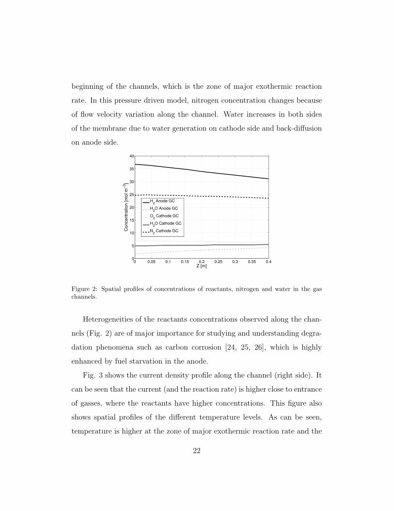
beginning of the channels, which is the zone of major exothermic reaction

rate. In this pressure driven model, nitrogen concentration changes because

of flow velocity variation along the channel. Water increases in both sides

of the membrane due to water generation on cathode side and back-diffusion

on anode side.

0 0.05 0.1 0.15 0.2 0.25 0.3 0.35 0.40

5

10

15

20

25

30

35

40

Z [m]

Concentr

atio

n [

mol m

−3]

H2 Anode GC

H2O Anode GC

O2 Cathode GC

H2O Cathode GC

N2 Cathode GC

Figure 2: Spatial profiles of concentrations of reactants, nitrogen and water in the gaschannels.

Heterogeneities of the reactants concentrations observed along the chan-

nels (Fig. 2) are of major importance for studying and understanding degra-

dation phenomena such as carbon corrosion [24, 25, 26], which is highly

enhanced by fuel starvation in the anode.

Fig. 3 shows the current density profile along the channel (right side). It

can be seen that the current (and the reaction rate) is higher close to entrance

of gasses, where the reactants have higher concentrations. This figure also

shows spatial profiles of the different temperature levels. As can be seen,

temperature is higher at the zone of major exothermic reaction rate and the

22

temperature of the gas channels follows the SP temperature.

0 0.05 0.1 0.15 0.2 0.25 0.3 0.35 0.4344

346

348

350

352

354

Z [m]

Te

mpe

ratu

re [K

]

560

580

600

620

640

660

Mem

bra

ne

Curr

ent

Den

sity [A

m−

2]

Anode GCCathode GCSolid PartT CoolMemb. Current Dens.

Figure 3: Spatial profiles of membrane current density and temperature in the gas chan-nels, solid part and cooling level.

Pressure variations cause nitrogen concentration to decrease but nitrogen

flow rate (not shown) is actually constant (35 mol m-2 s-1), because nitrogen

is not a reactant. Due to boundary conditions and a relatively small number

of mesh points, spatial profiles close to the inlet of gas channel are not very

smooth.

Fig. 4 shows spatial profiles for membrane water content, together with

spatial profiles of water transport from membrane to anode and cathode

catalyst layers.

As expected, membrane water content is higher at the end of the z direc-

tion and water is transported from both sides of membrane to the catalyst

layers due to water generated, electroosmotic drag and water diffusion. This

agrees with the results shown in Fig. 2, where water concentration increases

towards the end of the channel on both sides of the membrane.

23

0 0.05 0.1 0.15 0.2 0.25 0.3 0.35 0.46.2

6.3

6.4

6.5

6.6

6.7

6.8

6.9

7

Me

mb

ran

e W

ate

r C

on

ten

t [m

ol H

2O

/ m

ol p

oly

me

r]

0.6

0.8

1

1.2

1.4

1.6

1.8

2

2.2x 10

−3

Wa

ter

Flu

x [

mo

l m

−2 s

−1]

Z [m]

Water Membrane−Anode

Water Membrane−Cathode

Membrane Water Content

Figure 4: Spatial profiles of membrane water content, water transport from membrane toanode and cathode catalyst catalyst layers.

Finally, Fig. 5 shows a polarization curve obtained from the simulation

tool, in order to show its capacity to study experimental observables. Normal

values for PEMFC operation result for the range of operating conditions

considered in this i-V example.

0 1000 2000 3000 4000 5000 6000 70000.6

0.65

0.7

0.75

0.8

0.85

0.9

0.95

1

Current Density [A/m2]

Vo

lta

ge

[V

]

Figure 5: Polarization curve

24

5.2. Simulation results for step changes

At time t = 10 s the inflow of oxygen is increased up to 14 mol m−2 s−1

for 100 s, then at time t = 210 s, inflow of hydrogen is changed up to 12

mol m−2 s−1 for 100 s and finally, water inflow in the cathode is changed

down to 6 mol m−2 s−1. Fig. 6 shows the results of time variation of reactant

and water concentrations for the middle point of the channel.

0 100 200 300 400 5000

10

20

30

40

t [s]

H2 a

nd O

2 C

on

c. [m

ol m

−3]

2

3

4

5

6

H2O

Con

c. [m

ol m

−3]

H2O Conc. Cathode

H2 Conc.

H2O Conc. Anode

O2 Conc.

Figure 6: Time evolution of reactant and water concentration at the middle point of thechannel.

Fig. 7 shows the same type of diagram for membrane current density and

membrane water content, but considering three points along the channel. The

increase in reactants concentrations effectively increases membrane current

density and water content. It is important to notice the different response

of the system depending on the channel point. Changes at the first point of

the channel are almost immediate, whereas there is a slower time constant

further along the channel.

25

0 50 100 150 200 250 300 350 400 450 500 5506

6.5

7

7.5

t [s]

Mem

bra

ne W

ate

r C

onte

nt

500

600

700

800

Mem

bra

ne C

urr

ent D

ensity [A

m2−]

z = 0mz = 0.2mz = 0.4mz = 0mz = 0.2mz = 0.4m

Figure 7: Time evolution of membrane water content and current density at the beginningpoint, middle point and channel end. Black lines correspond to membrane current density.

6. Conclusions

A two-dimensional PEMFC simulation tool, suitable for along-the-channel

studies, has been developed in Matlab R©. The tool is flexible enough to ap-

ply order reduction techniques and to be used in model-based control design.

Simulation results show the importance of considering, and therefore, con-

trolling aspects of spatial profiles, especially for PEMFC performance and

durability issues. It is the intention of the authors to make the source code

publicly available.

Acknowledgements

This work has been supported by national projects DISCPICO with refer-

ence DPI2010-15274, MESPEM with reference DPI2011-25649 and european

project PUMA MIND.

26

References

[1] I. S. A. I. C. Parsons, Fuel Cell Handbook, U.S. Department of Energy,

2000.

[2] D. Bernardi, M. Verbrugge, Mathematical model of a gas diffusion

electrode bonded to polymer electrolyte, AIChE 37 (1991).

[3] C. Siegel, Review of computational heat and mass transfer modeling

in polymer-electrolyte-membrane (PEM) fuel cells, Energy 33 (2008)

1331–1352.

[4] A. Rowe, X. Li, Mathematical modeling of proton exchange membrane

fuel cells, Journal of Power Sources 102 (2001) 82–96.

[5] R. Methekar, V. Prasad, R. Gudi, Dynamic analysis and linear control

strategies for proton exchange membrane fuel cell using a distributed

parameter model, Journal of Power Sources 165 (2007) 152–170.

[6] M. Mangold, A. Buck, R. Hanke-Rauschenbach, Passivity based control

of a distributed pem fuel cell model, Journal of Process Control 20

(2010) 292–313.

[7] S. Um, C. Y. Wang, K. S. Chen, Computational fluid dynamics modeling

of proton exchange membrane fuel cells, Journal of The Electrochemical

Society 147 (2000) 4485–4493.

[8] A. Kulikovsky, Semi-analytical 1D + 1D model of a polymer electrolyte

fuel cell, Electrochemistry Communications 6 (2004) 969 – 977.

27

[9] M. H. Nehrir, C. Wang, Modeling and Control of Fuel Cells: Distributed

Generation Applications, Wiley-IEEE Press, 2009.

[10] J. Schumacher, J. Eller, G. Sartoris, A 2 + 1D model of a proton

exchange membrane fuel cell with glassy-carbon micro-structures, in:

Proceedings MATHMOD, pp. 16–19.

[11] W. Tao, C. Min, X. Liu, Y. He, B. Yin, W. Jiang, Parameter sen-

sitivity examination and discussion of pem fuel cell simulation model

validation: Part i. current status of modeling research and model devel-

opment, Journal of Power Sources 160 (2006) 359–373.

[12] S. Um, C. Wang, Three-dimensional analysis of transport and electro-

chemical reactions in polymer electrolyte fuel cells, Journal of Power

Sources 125 (2004) 40 – 51.

[13] A. A. Franco, A multiscale modeling framework for the transient analysis

of PEM Fuel Cells - From the fundamentals to the engineering practice.,

Universite Claude Bernard Lyon 1, 2010.

[14] R. F. de Morais, P. Sautet, D. Loffreda, A. A. Franco, A multiscale the-

oretical methodology for the calculation of electrochemical observables

from ab initio data: Application to the oxygen reduction reaction in a

Pt(1 1 1)-based polymer electrolyte membrane fuel cell, Electrochimica

Acta 56 (2011) 10842 – 10856.

[15] A. A. Franco, P. Schott, C. Jallut, B. Maschke, A multi-scale dynamic

mechanistic model for the transient analysis of PEFCs, Fuel Cells 7

(2007) 99–117.

28

[16] COMSOL, Comsol, http://www.comsol.com/, 2012.

[17] E. Verriest, Time variant balancing and nonlinear balanced realizations,

in: W. H. A. Schilders, H. A. van der Vorst, J. Rommes (Eds.), Model

order reduction. Theory, research aspects and applications, Springer,

2008.

[18] W. Neubrand, Modellbildung und Sumulation von Elektromembranver-

fahren, Logos-Verlag, 1999.

[19] M. Wohr, Instationares, thermodynamisches Verhalten der

Polymermembra-Brennstoffzelle, VDI-Verlag, 1999.

[20] F. Barbir, PEM Fuel Cells: Theory and Practice, Academic Press, 2005.

[21] J. Sjoberg, Optimal control and model reduction of nonlinear DAE mod-

els, Ph.D. thesis, Linkoping University, Sweden, 2008.

[22] P. K. Kundu, I. M. Cohen, Fluid Mechanics, Academic Press, 1990.

[23] H. D. B. Jenkins, Chemical Thermodynamics at a Glance, Blackwell

Publishing, 2008.

[24] K. Malek, A. A. Franco, Microstructure-based modeling of aging mech-

anisms in catalyst layers of polymer electrolyte fuel cells, The Journal

of Physical Chemistry B 115 (2011) 8088–8101.

[25] A. A. Franco, M. Gerard, Transient model of carbon catalyst-support

corrosion in a PEFC: Multi-scale coupling with Pt electro-catalysis and

impact on performance degradation, Meeting Abstracts MA2008-01

(2008) 1160.

29

[26] J. Wu, X. Yuan, J. Martin, H. Wang, J. Zhang, J. Shen, S. Wu,

W. Merida, A review of pem fuel cell durability: Degradation mech-

anisms and mitigation strategies, Journal of Power Sources 184 (2008)

104–119.

30