Embed Size (px)
Citation preview

Algebraic Statistics for Computational Biology
Edited by
Lior Pachter and Bernd Sturmfels
CAG T


Contents
Preface page vii
Part I Introduction to the four themes 1
1 Statistics L. Pachter and B. Sturmfels 3
1.1 Statistical models for discrete data 4
1.2 Linear models and toric models 9
1.3 Expectation maximization 17
1.4 Markov models 25
1.5 Graphical models 35
2 Computation L. Pachter and B. Sturmfels 45
2.1 Tropical arithmetic and dynamic programming 46
2.2 Sequence alignment 52
2.3 Polytopes 61
2.4 Trees and metrics 71
2.5 Software 79
3 Algebra L. Pachter and B. Sturmfels 90
3.1 Varieties and Grobner bases 91
3.2 Implicitization 100
3.3 Maximum likelihood estimation 109
3.4 Tropical geometry 115
3.5 The tree of life and other tropical varieties 125
4 Biology L. Pachter and B. Sturmfels 133
4.1 Genomes 134
4.2 The data 140
4.3 The questions 146
4.4 Statistical models for a biological sequence 149
4.5 Statistical models of mutation 156
iii

iv Contents
Part II Studies on the four themes 167
5 Parametric Inference R. Mihaescu 171
5.1 Tropical sum-product decompositions 172
5.2 The Polytope Propagation Algorithm 176
5.3 Algorithm Complexity 180
5.4 Specialization of Parameters 184
6 Polytope Propagation on Graphs M. Joswig 188
6.1 Introduction 188
6.2 Polytopes from Directed Acyclic Graphs 189
6.3 Specialization to Hidden Markov Models 192
6.4 An Implementation in polymake 194
6.5 Returning to Our Example 199
7 Parametric Sequence Alignment
C. Dewey and K. Woods 200
7.1 Few alignments are optimal 200
7.2 Polytope propagation for alignments 202
7.3 Retrieving alignments from polytope vertices 206
7.4 Achieving biological correctness 210
8 Bounds for Optimal Sequence Alignment
S. Elizalde and F. Lam 213
8.1 Alignments and optimality 213
8.2 Geometric Interpretation 214
8.3 Known bounds 218
8.4 The Square Root Conjecture 219
9 Inference Functions S. Elizalde 222
9.1 What is an inference function? 222
9.2 The Few Inference Functions Theorem 223
9.3 Inference functions for sequence alignment 226
10 Geometry of Markov Chains E. Kuo 232
10.1 Viterbi Sequences 232
10.2 Two- and Three-State Markov Chains 234
10.3 Markov Chains with Many States 236
10.4 Fully Observed Markov Models 238
11 Equations Defining Hidden Markov Models
N. Bray and J. Morton 242
11.1 The Hidden Markov Model 242
11.2 Grobner Bases 243
11.3 Linear Algebra 245
11.4 Invariant Interpretation 252

Contents v
12 The EM Algorithm for Hidden Markov Models
I. B. Hallgrımsdottir, R. A. Milowski and J. Yu 255
12.1 The Baum-Welch algorithm 255
12.2 Evaluating the likelihood function 263
12.3 A general discussion about the EM algorithm 266
13 Homology mapping with Markov Random Fields A. Caspi 270
13.1 Genome mapping 270
13.2 Markov random fields 272
13.3 MRFs in homology assignment 276
13.4 Tractable MAP Inference in a subclass of MRFs 279
13.5 The Cystic Fibrosis Transmembrane Regulator 282
14 Mutagenetic Tree Models N. Beerenwinkel and M. Drton 284
14.1 Accumulative Evolutionary Processes 284
14.2 Mutagenetic Trees 285
14.3 Mixture Models 294
15 Catalog of Small Trees
M. Casanellas, L. D. Garcia, and S. Sullivant 298
15.1 Notational Conventions 298
15.2 Description of website features 305
15.3 Example 305
15.4 Using the invariants 308
16 The Strand Symmetric Model
M. Casanellas and S. Sullivant 312
16.1 Introduction 312
16.2 Matrix-Valued Fourier Transform 313
16.3 Invariants for the 3 taxa tree 318
16.4 G-tensors 322
16.5 Extending invariants 327
16.6 Reduction to K1,3 328
17 Extending Tree Models to Split Networks D. Bryant 331
17.1 Introduction 331
17.2 Trees, splits and split networks 332
17.3 Distance based models for trees and splits graphs 335
17.4 A graphical model on a splits network? 337
17.5 Group based mutation models 338
17.6 Group based models on trees and splits 340
17.7 A Fourier calculus for split networks 342
17.8 Discussion 345
vi Contents
18 Small Trees and Generalized Neighbor-Joining
M. Contois and D. Levy 347
18.1 From Alignments to Dissimilarity 347
18.2 From Dissimilarity to Trees 349
18.3 The Need for Exact Solutions 354
18.4 Jukes-Cantor Triples 357
19 Tree Construction Using Singular Value Decomposition
N. Eriksson 360
19.1 The General Markov Model 360
19.2 Flattenings and Rank Conditions 361
19.3 Singular Value Decomposition 364
19.4 Tree Construction Algorithm 365
19.5 Performance Analysis 368
20 Applications of Interval Methods to Phylogenetics
R. Sainudiin and R. Yoshida 373
20.1 Interval methods for exact solutions 373
20.2 Enclosing the likelihood of a compact set of trees 380
20.3 Global Optimization 381
20.4 Applications to phylogenetics 386
21 Analysis of Point Mutations in Vertebrate Genomes
J. Al-Aidroos and S. Snir 390
21.1 Estimating mutation rates 390
21.2 The ENCODE data 393
21.3 Synonymous substitutions 395
21.4 The rodent problem 397
22 Ultra-Conserved Elements in Vertebrate and Fly Genomes
M. Drton, N. Eriksson and G. Leung 403
22.1 The Data 403
22.2 Ultra-Conserved Elements 405
22.3 Biology of Ultra-Conserved Elements 408
22.4 Probability of Ultra-Conservation 416
Index 437
Preface
The title of this book reflects who we are: a computational biologist and an
algebraist who share a common interest in statistics. Our collaboration sprang
from the desire to find a mathematical language for discussing biological se-
quence analysis, with the initial impetus being provided by the Introductory
Workshop on Discrete and Computational Geometry at the Mathematical Sci-
ences Research Institute (MSRI) held at Berkeley in August 2003. At that
workshop we began exploring the similarities between tropical matrix multi-
plication and the Viterbi algorithm for hidden Markov models. Our discussions
ultimately led to two articles [Pachter and Sturmfels, 2004a,b] which are ex-
plained and further developed in various chapters of this book.
In the fall of 2003 we held a graduate seminar on The Mathematics of
Phylogenetic Trees. About half of the authors in the second part of this
book already participated in that seminar. It was based on topics from the
books [Felsenstein, 2003, Semple and Steel, 2003] but we also discussed other
projects, such as Michael Joswig’s polytope propagation on graphs (now Chap-
ter 6). That seminar got us up to speed on research topics in phylogenetics, and
led us to participate in the conference on Phylogenetic Combinatorics which
was held in July 2004 in Uppsala, Sweden. In Uppsala we were introduced to
David Bryant and his statistical models for split systems (now Chapter 17).
Another milestone was the workshop on Computational Algebraic Statistics
which was held at the American Institute for Mathematics (AIM) at Palo
Alto in December 2003. That workshop was built on the algebraic statistics
paradigm, which is that statistical models for discrete data can be represented
as solutions to systems of polynomial equations. Our current understanding of
algebraic statistical models, maximum likelihood estimation and expectation
maximization was shaped by the excellent lectures and discussions at AIM.
These developments led us to offer a mathematics graduate course titled Al-
gebraic Statistics for Computational Biology in the fall of 2004. The course was
attended mostly by mathematics students curious about computational biol-
vii

viii Preface
ogy, but also by computer scientists, statisticians, and bioengineering students
interested in understanding the mathematical foundations of bioinformatics.
Participants ranged from senior postdocs to first year graduate students and
even one undergraduate. The format consisted of lectures by us on basic
principles of algebraic statistics and computational biology, as well as student
participation in the form of group projects and presentations. The class was
divided into four sections, reflecting the four themes of algebra, statistics, com-
putation and biology. Each group was assigned a handful of projects to pursue,
with the goal of completing a written report by the end of the semester. In
some cases the groups worked on the problems we suggested, but, more often
than not, original ideas by group members led to independent research plans.
Half way through the semester, it became clear that the groups were making
fantastic progress, and that their written reports would contain many novel
ideas and results. At that point, we thought about preparing a book. The
first half of the book would be based on our own lectures, and the second half
would consist of chapters based on the final term papers. A tight schedule
was seen as essential for the success of such an undertaking, given that many
participants would be leaving Berkeley and the momentum would be lost. It
was decided that the book should be written by March 2005, or not at all.
We were fortunate to find a partner in Cambridge University Press, which
agreed to work with us on our concept. We are especially grateful to our editor,
David Tranah, for his strong encouragement, and his trust that our half-baked
ideas could actually turn into a readable book. After all, we were proposing
to write to a book with twenty-nine authors during a period of three months.
The project did become reality and the result is in your hands. It offers an
accurate snapshot of what happened during our seminars at UC Berkeley in
2003 and 2004. Nothing more and nothing less. The choice of topics is certainly
biased, and the presentation is undoubtedly very far from perfect. But we hope
that it may serve as an invitation to biology for mathematicians, and as an
invitation to algebra for biologists, statisticians and computer scientists.
We acknowledge the National Science Foundation and the National Insti-
tute of Health for their financial support, and many friends and colleagues for
providing helpful comments – there are far too many to list individually. Most
of all, we are grateful to our wonderful students and postdocs from whom we
learned so much. Their enthusiasm and hard work have been truly amazing.
You will enjoy meeting them in Part 2.
Lior Pachter and Bernd Sturmfels
Berkeley, California, March 2005
Part I
Introduction to the four themes
Part I of this book is devoted to outlining the basic principles of algebraic
statistics, and their relationship to computational biology. Although some of
the ideas are complex, and their relationships intricate, the underlying phi-
losophy of our approach to biological sequence analysis is summarized in the
cartoon on the cover of the book. The fictional character is DiaNA, who
appears throughout the book, and who is the statistical surrogate for our bio-
logical intuition. In the cartoon, DiaNA is walking randomly on a graph and
she is throwing tetrahedral dice that can land on one of the characters A,C,G
or T. A key feature of the tosses is that the outcome depends on the direction
she is walking. We, the observers, record the characters that appear on the
successive throws, but are unable to see the path that DiaNA takes on her
graph. Our goal is to guess DiaNA’s path from the die roll outcomes. That is,
we wish to make an inference about missing data from certain observed data.
In this book, the observed data are DNA sequences, and in Chapter 4 we
explain the relevance of the example depicted on the cover to the biological
problem of sequence alignment. The tetrahedral shape of the die hint at poly-
topes, which we see in Chapter 2 are fundamental geometric objects that play
a key role in making guesses about DiaNA. Underlying the whole story is al-
gebra, featured in Chapter 3, and which is the universal language with which
to describe the underlying process at the heart of DiaNA’s randomness.
Chapter 1 offers a fairly self-contained introduction to algebraic statistics.
Many concepts of statistics have a natural analog in algebraic geometry, and
there is an emerging dictionary which bridges the gap between these disciplines:
independence = Segre variety
exponential family = toric variety
curved exponential family = manifold
mixture model = secant variety
inference = tropicalization
· · · · · · = · · · · · · · · ·
This dictionary is far from complete and finished, but it already suggests that
algorithmic tools from algebraic geometry, most notably Grobner bases, may
be used for computations in statistics that may be beneficial for computational
biology applications. While we are well aware of the limitations of algebraic
2
algorithms, with Grobner bases computations typically becoming intractable
beyond toy problems, we nevertheless believe that computational biologists
might benefit from adding the techniques described in Chapter 3 to their tool
box. In addition, we have found the algebraic point of view to be useful in
unifying and developing many computational biology algorithms. For example,
the results on parametric sequence alignment in Chapter 7 do not require
the language of algebra to be understood or utilized, but were motivated by
concepts such as the Newton polytope of a polynomial. Chapter 2 discusses
discrete algorithms which provide efficient solutions to various problems of
statistical inference. Chapter 4 is an introduction to the biology, where we
return to many of the examples in Chapter 1, illustrating how the statistical
models we have discussed play a prominent role in computational biology.
We emphasize that Part I serves mainly as an introduction and reference
for the chapters in Part II. We have therefore omitted many topics which are
rightfully considered to be an integral part of computational biology. For ex-
ample, we have restricted ourselves to the topic of biological sequence analysis,
and within that domain have focused on eukaryotic genome analysis. Read-
ers interested in a more complete introduction to computational biology are
referred to [Durbin et al., 1998], our favorite introduction to the area. Also
useful may be a text on molecular biology with an emphasis on genomics, such
as [Brown, 2002]. Our treatment of computational algebra in Chapter 3 is only
a sliver taken from a mature and developed subject. The excellent book by
[Cox et al., 1997] fills in many of the details missing in our discussions.
Because Part I covers many topics, a comprehensive list of prerequisites
would include a background in computer science, familiarity with molecular
biology, and the benefit of having taken introductory courses in statistics and
abstract algebra. Direct experience in computational biology would also be
desirable. Of course, we recognize that this is asking too much. Real-life
readers may be experts in one of these subjects but completely unfamiliar
with others, and we have taken this into account when writing the book.
Various chapters provide natural points of entry for readers with different
backgrounds. Those wishing to learn more about genomes can start with
Chapter 4, biologists interested in software tools can start with Section 2.5,
and statisticians who wish to brush up their algebra can start with Chapter 3.
In summary, the book is not meant to serve as the definitive text for algebraic
statistics or computational biology, but rather as a first invitation to biology
for mathematicians, and conversely as a mathematical primer for biologists.
In other words, it is written in the spirit of interdisciplinary collaboration that
is highlighted in the article Mathematics is Biology’s Next Microscope, Only
Better; Biology is Mathematics’ Next Physics, Only Better [Cohen, 2004].
1
Statistics
Lior Pachter
Bernd Sturmfels
Statistics is the science of data analysis. The data to be encountered in this
book are derived from genomes. Genomes consist of long chains of DNA which
are represented by sequences in the letters A, C, G or T. These abbreviate the
four nucleic acids Adenine, Cytosine, Guanine and Thymine, which serve as
fundamental building blocks in biology.
What do statisticians do with their data? They build models of the process
that generated the data and, in what is known as statistical inference, draw con-
clusions about this process. Genome sequences are particularly interesting data
to draw conclusions from: they are the blueprint for life, and yet their function,
structure, and evolution are poorly understood. Statistics is fundamental for
genomics, a point of view that was emphasized in [Durbin et al., 1998].
The inference tools we present in this chapter look different from those found
in [Durbin et al., 1998], or most other texts on computational biology or math-
ematical statistics: they are written in the language of abstract algebra. The
algebraic language for statistics clarifies many of the ideas central to analysis
of discrete data, and, within the context of biological sequence analysis, unifies
the main ingredients of many widely used algorithms.
Algebraic Statistics is a new field, less than a decade old, whose precise scope
is still emerging. The term itself was coined by Giovanni Pistone, Eva Ricco-
magno and Henry Wynn, with the title of their book [Pistone et al., 2001].
That book explains how polynomial algebra arises in problems from experi-
mental design and discrete probability, and it demonstrates how computational
algebra techniques can be applied to statistics.
This chapter takes some additional steps along the algebraic statistics path.
It offers a self-contained introduction to algebraic statistical models, with the
aim of developing inference tools necessary for studying genomes. Special
emphasis will be placed on (hidden) Markov models and graphical models.
3
4 L. Pachter and B. Sturmfels
1.1 Statistical models for discrete data
Imagine a fictional character named DiaNA who produces sequences of letters
over the four-letter alphabet A, C, G, T. An example of such a sequence is
CTCACGTGATGAGAGCATTCTCAGACCGTGACGCGTGTAGCAGCGGCTC (1.1)
The sequences produced by DiaNA are called DNA sequences. DiaNA gen-
erates her sequences by some random process. When modeling this random
process we make assumptions about part of its structure. The resulting sta-
tistical model is a family of probability distributions, one of which we believe
governs the process by which DiaNA generates her sequences. In this book we
consider parametric statistical models, which are families of probability dis-
tributions that can be parameterized by a finite-dimensional parameter. One
important task is to estimate DiaNA’s parameters from the sequences she gen-
erates. Estimation is also called learning in the computer science literature.
DiaNA uses tetrahedral dice to generate DNA sequences. Each tetrahedral
die has the shape of a tetrahedron, and its four faces are labeled with the
letters A, C, G and T. If DiaNA rolls a fair die then each of the four letters will
appear with the same probability 1/4. If she uses a loaded tetrahedral die then
the four probabilities can be any four non-negative numbers that sum to one.
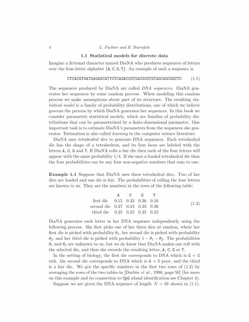
Example 1.1 Suppose that DiaNA uses three tetrahedral dice. Two of her
dice are loaded and one die is fair. The probabilities of rolling the four letters
are known to us. They are the numbers in the rows of the following table:
A C G T
first die 0.15 0.33 0.36 0.16
second die 0.27 0.24 0.23 0.26
third die 0.25 0.25 0.25 0.25
(1.2)
DiaNA generates each letter in her DNA sequence independently using the
following process. She first picks one of her three dice at random, where her
first die is picked with probability θ1, her second die is picked with probability
θ2, and her third die is picked with probability 1 − θ1 − θ2. The probabilities
θ1 and θ2 are unknown to us, but we do know that DiaNA makes one roll with
the selected die, and then she records the resulting letter, A, C, G or T.
In the setting of biology, the first die corresponds to DNA which is G + C
rich. the second die corresponds to DNA which is G + C poor, and the third
is a fair die. We got the specific numbers in the first two rows of (1.2) by
averaging the rows of the two tables in [Durbin et al., 1998, page 50] (for more
on this example and its connection to CpG island identification see Chapter 4).
Suppose we are given the DNA sequence of length N = 49 shown in (1.1).
Statistics 5
One question that may be asked is whether the sequence was generated by
DiaNA using this process, and, if so, which parameters θ1 and θ2 did she use?
Let pA, pC, pG and pT denote the probabilities that DiaNA will generate
any of her four letters. The statistical model we have discussed is written in
algebraic notation as
pA = −0.10 · θ1 + 0.02 · θ2 + 0.25,
pC = 0.08 · θ1 − 0.01 · θ2 + 0.25,
pG = 0.11 · θ1 − 0.02 · θ2 + 0.25,
pT = −0.09 · θ1 + 0.01 · θ2 + 0.25.
Note that pA+pC +pG +pT = 1, and we get the three distributions in the rows
of (1.2) by specializing (θ1, θ2) to (1, 0), (0, 1) and (0, 0) respectively.
To answer our questions, we consider the likelihood of observing the partic-
ular data (1.1). Since each of the 49 characters was generated independently,
that likelihood is the product of the probabilities of the individual letters:
L = pCpTpApCpCpG · · ·pA = p10A · p14
C · p15G · p10
T .
This expression is the likelihood function of DiaNA’s model for the data (1.1).
To stress the fact that the parameters θ1 and θ2 are unknowns we write
L(θ1, θ2) = pA(θ1, θ2)10 · pC(θ1, θ2)14 · pG(θ1, θ2)15 · pT(θ1, θ2)10.
This likelihood function is a real-valued function on the triangle
Θ =(θ1, θ2) ∈ R2 : θ1 > 0 and θ2 > 0 and θ1 + θ2 < 1
.
In the paradigm of maximum likelihood we estimate the parameter values that
DiaNA used by those values which make the likelihood of observing her data
as large as possible. Thus our task is to maximize L(θ1, θ2) over the triangle
Θ. It is equivalent but more convenient to maximize the log-likelihood function
ℓ(θ1, θ2) = log(L(θ1, θ2)
)
= 10 · log(pA(θ1, θ2)) + 14 · log(pC(θ1, θ2))
+ 15 · log(pG(θ1, θ2)) + 10 · log(pT(θ1, θ2)).
The solution to this optimization problem can be computed in closed form, by
equating the two partial derivatives of the log-likelihood function to zero:
∂ℓ
∂θ1=
10
pA· ∂pA∂θ1
+14
pC· ∂pC∂θ1
+15
pG· ∂pG∂θ1
+10
pT· ∂pT∂θ1
= 0,
∂ℓ
∂θ2=
10
pA· ∂pA∂θ2
+14
pC· ∂pC∂θ2
+15
pG· ∂pG∂θ2
+10
pT· ∂pT∂θ2
= 0.
Each of the two expressions is a rational function in (θ1, θ2). By clearing de-
nominators and by applying the algebraic technique of Grobner bases (Section
6 L. Pachter and B. Sturmfels
3.1), we can transform the two equations above into the equivalent equations
13003050 · θ1 + 2744 · θ22 − 2116125 · θ2 − 6290625 = 0,
134456 · θ32 − 10852275 · θ22 − 4304728125 · θ2 + 935718750 = 0.(1.3)
The second equation has a unique solution θ2 between 0 and 1. The corre-
sponding value of θ1 is obtained by solving the first equation. Approximately,
(θ1, θ2) =(0.5191263945, 0.2172513326
).
The log-likelihood function attains its maximum value at this point:
ℓ(θ1, θ2) = −67.08253037.
The corresponding probability distribution
(pA, pC, pG, pT) =(0.202432, 0.289358, 0.302759, 0.205451
)(1.4)
is very close (in a statistical sense [Bickel, 1971]) to the empirical distribution
1
49(10, 14, 15, 10) =
(0.204082, 0.285714, 0.306122, 0.204082
). (1.5)
We conclude that the proposed model is a good fit for the data (1.1) and guess
that DiaNA used the probabilities θ1 and θ2 for choosing among her dice.
We now turn to our general discussion of statistical models for discrete data.
A statistical model is a family of probability distributions on some state space.
In this book we assume that the state space is finite, but possibly quite large.
We often identify the state space with the set of the first m positive integers,
[m] := 1, 2, . . . , m. (1.6)
A probability distribution on the set [m] is a point in the probability simplex
∆m−1 :=
(p1, . . . , pm) ∈ Rm :
m∑
i=1
pi = 1 and pj ≥ 0 for all j. (1.7)
The index m − 1 indicates the dimension of the simplex ∆m−1. We write ∆
for the simplex ∆m−1 when the underlying state space [m] is understood.
Example 1.2 The state space for DiaNA’s dice is the set A, C, G, T which
we identify with the set [4] = 1, 2, 3, 4. The simplex ∆ is a tetrahedron.
The probability distribution associated with a fair die is the point (14 ,
14 ,
14 ,
14),
which is the centroid of the tetrahedron ∆. Equivalently, we may think about
our model via the concept of a random variable, that is a function X taking
values in the state space A, C, G, T . Then the point corresponding to a fair die
gives the probability distribution of X as Prob(X = A) = 14 , Prob(X = C) =
Statistics 7
14 , Prob(X = G) = 1
4 , Prob(X = T) = 14 . All other points in the tetrahedron
∆ correspond to loaded dice.
A statistical model for discrete data is a family of probability distributions
on [m]. Equivalently, a statistical model is simply a subset of the simplex
∆. The i-th coordinate pi represents the probability of observing the state i,
and in that capacity pi must be a non-negative real number. However, when
discussing algebraic computations (as in Chapter 3), we sometimes relax this
requirement and allow pi to be negative or even a complex number.
An algebraic statistical model arises as the image of a polynomial map
f : Rd → Rm , θ = (θ1, . . . , θd) 7→(f1(θ), f2(θ), . . . , fm(θ)
). (1.8)
The unknowns θ1, . . . , θd represent the model parameters. In most cases of
interest, d is much smaller than m. Each coordinate function fi is a polynomial
in the d unknowns, which means it has the form
fi(θ) =∑
a∈Nd
ca · θa11 θa2
2 · · ·θadd , (1.9)
where all but finitely many of the coefficients ca ∈ R are zero. We use N to
denote the non-negative integers, that is, N = 0, 1, 2, 3, . . ..The parameter vector (θ1, . . . , θd) ranges over a suitable non-empty open
subset Θ of Rd which is called the parameter space of the model f . We assume
that the parameter space Θ satisfies the condition
fi(θ) > 0 for all i ∈ [m] and θ ∈ Θ (1.10)
Under these hypotheses, the following two conditions are equivalent:
f(Θ) ⊆ ∆ ⇐⇒ f1(θ) + f2(θ) + · · ·+ fm(θ) = 1 (1.11)
This is an identity of polynomial functions, which means that all non-constant
terms of the polynomials fi cancel, and the constant terms add up to 1. If
(1.11) holds, then our model is simply the set f(Θ).
Example 1.3 DiaNA’s model in Example 1.1 is a mixture model which mixes
three distributions on A, C, G, T. Geometrically, the image of DiaNA’s map
f : R2 → R4 , (θ1, θ2) 7→ (pA, pC, pG, pT)
is the plane in R4 which is cut out by the two linear equations
pA + pC + pG + pT = 1 and 11 pA + 15 pG = 17 pC + 9 pT. (1.12)
This plane intersects the tetrahedron ∆ in the quadrangle whose vertices are
(0, 0,
3
8,5
8
),(0,
15
32,17
32, 0),( 9
20, 0, 0,
11
20
)and
(17
28,11
28, 0, 0
). (1.13)

8 L. Pachter and B. Sturmfels
Inside this quadrangle is the triangle f(Θ) whose vertices are the three rows of
the table in (1.2). The point (1.4) lies in that triangle and is near (1.5).
Some statistical models are naturally given by a polynomial map f for which
(1.11) does not hold. If this is the case then we scale each vector in f(Θ) by
the positive quantity∑m
i=1 fi(θ). Regardless of whether (1.11) holds or not,
our model is the family of all probability distributions on [m] of the form
1∑mi=1 fi(θ)
·(f1(θ), f2(θ), . . . , fm(θ)
)where θ ∈ Θ. (1.14)
We generally try to keep things simple and assume that (1.11) holds. However,
there are some cases, such as the general toric model in the next section, when
the formulation in (1.14) is more natural. It poses no great difficulty to extend
our theorems and algorithms from polynomials to rational functions.
Our data are typically given in the form of a sequence of observations
i1, i2, i3, i4, . . . , iN . (1.15)
Each data point ij is an element from our state space [m]. The integerN , which
is the length of the sequence, is called the sample size. We summarize the data
(1.15) in the data vector u = (u1, u2, . . . , um) where uk is the number of indices
j ∈ [N ] such that ij = k. Hence u is a vector in Nm with u1+u2+· · ·+um = N .
The empirical distribution corresponding to the data (1.15) is the scaled vector1N u which is a point in the probability simplex ∆. The coordinates ui/N of
the vector 1N u are the observed frequencies of the various possible outcomes.
We consider the model f to be a “good fit” for the data u if there exists a
parameter vector θ ∈ Θ such that the probability distribution f(θ) is very close,
in a statistically meaningful sense [Bickel, 1971], to the empirical distribution1N u. Suppose we independently draw N times at random from the set [m] with
respect to the probability distribution f(θ). Then the probability of observing
the sequence (1.15) equals
L(θ) = fi1(θ)fi2(θ) · · ·fiN (θ) = f1(θ)u1 · · ·fm(θ)um . (1.16)
This expression depends on the parameter vector θ as well as the data vector
u. However, we think of u as being fixed and then L is a function from Θ to the
positive real numbers. It is called the likelihood function to emphasize that it
is a function that depends on θ, and to distinguish it from an expression for a
probability. Note that any reordering of the sequence (1.15) leads to the same
data vector u. Hence the probability of observing the data vector u is equal to
(u1 + u2 + · · ·+ um)!
u1!u2! · · ·um!· L(θ). (1.17)
The vector u plays the role of a sufficient statistic for the model f . This means
Statistics 9
that the likelihood function L(θ) depends on the data (1.15) only through u.
In practice one often replaces the likelihood function by its logarithm
ℓ(θ) = logL(θ) = u1·log(f1(θ))+u2·log(f2(θ))+· · ·+um·log(fm(θ)). (1.18)
This is the log-likelihood function. Note that ℓ(θ) is a function from the pa-
rameter space Θ ⊂ Rd to the negative real numbers R<0.
The problem of maximum likelihood estimation is to maximize the likelihood
function L(θ) in (1.16), or, equivalently, the scaled likelihood function (1.17),
or, equivalently, the log-likelihood function ℓ(θ) in (1.18). Here θ ranges over
the parameter space Θ ⊂ Rd. Formally, we consider the optimization problem:
Maximize ℓ(θ) subject to θ ∈ Θ. (1.19)
A solution to this optimization problem is denoted θ and is called a maximum
likelihood estimate of θ with respect to the model f and the data u. Sometimes,
if the model satisfies certain properties, it may be that the maximum likelihood
estimate θ is always unique. This happens for linear models and toric models,
due to the concavity of their log-likelihood function, as we shall see in Section
1.2. For most statistical models, however, the situation is not as simple. There
can be more than one global maximum, in fact, there can be infinitely many of
them. And it may be difficult to find any one of these global maxima. In that
case, one may content oneself with a local maximum of the likelihood function.
In Section 1.3 we shall discuss the EM algorithm which is a numerical method
for finding solutions to the maximum likelihood estimation problem (1.19).
1.2 Linear models and toric models
In this section we introduce two classes of models which have the property that
maximum likelihood estimation (1.19) is a convex optimization problem. As-
suming that the parameter domain Θ is bounded, it follows that the likelihood
function has exactly one local maximum θ ∈ Θ, and it is easy to numerically
compute the maximum likelihood estimate θ using any of the hill-climbing
methods of convex optimization, such as the gradient ascent algorithm.
1.2.1 Linear models
An algebraic statistical model f : Rd → Rm is called a linear model if each of
its coordinate polynomials fi(θ) is a linear function. Being a linear function
means there exist real numbers ai1, . . . , a1d and bi such that
fi(θ) =
d∑
j=1
aijθj + bi. (1.20)
10 L. Pachter and B. Sturmfels
The m linear functions f1(θ), . . . , fm(θ) have the property that their sum is the
constant function 1. DiaNA’s model studied in Example 1.1 is a linear model.
For the data discussed in that example, the log-likelihood function ℓ(θ) had a
unique local maximum on the parameter triangle Θ. The following proposition
states that this desirable property holds for every linear model.
Proposition 1.4 For any linear model f and data u ∈ Nm, the log-likelihood
function ℓ(θ) =∑m
i=1 ui log(fi(θ)) is concave. If the linear map f is one-to-
one and all ui are positive then the log-likelihood function is strictly concave.
Proof Our assertion that the log-likelihood function ℓ(θ) is concave states
that the Hessian matrix(
∂2ℓ∂θj ∂θk
)is negative semi-definite. In other words, we
need to show that every eigenvalue of this symmetric matrix is non-positive.
The partial derivative of the linear function fi(θ) in (1.20) with respect to
the unknown θj is the constant aij . Hence the partial derivative of the log-
likelihood function ℓ(θ) equals
∂ℓ
∂θj=
m∑
i=1
uiaij
fi(θ). (1.21)
Taking the derivative again, we get the following formula for the Hessian matrix(
∂2ℓ
∂θj ∂θk
)= −AT · diag
(u1
f1(θ)2,
u2
f2(θ)2, . . . ,
um
fm(θ)2
)·A. (1.22)
Here A is the m × d matrix whose entry in row i and column j equals aij.
This shows that the Hessian (1.22) is a symmetric d× d matrix each of whose
eigenvalues is non-positive.
The argument above shows that ℓ(θ) is a concave function. Moreover, if the
linear map f is one-to-one then the matrix A has rank d. In that case, provided
all ui are strictly positive, all eigenvalues of the Hessian are strictly negative,
and we conclude that ℓ(θ) is strictly concave for all θ ∈ Θ.
The critical points of the likelihood function ℓ(θ) of the linear model f are
the solutions to the following system of d equations in d unknowns which are
obtained by equating (1.21) to zero. What we get are the likelihood equations
m∑
i=1
uiai1
fi(θ)=
m∑
i=1
uiai2
fi(θ)= · · · =
m∑
i=1
uiaid
fi(θ)= 0. (1.23)
The study of these equations involves the combinatorial theory of hyperplane
arrangements. Indeed, consider the m hyperplanes in d-space Rd which are
defined by the equations fi(θ) = 0 for i = 1, 2, . . . , m. The complement of this
arrangement of hyperplanes in Rd is the following set of parameter values
C =θ ∈ Rd : f1(θ)f2(θ)f3(θ) · · ·fm(θ) 6= 0
.
Statistics 11
This set is the disjoint union of finitely many open convex polyhedra defined by
inequalities fi(θ) > 0 or fi(θ) < 0. These polyhedra are called the regions of the
arrangement. Some of these regions are bounded, and others are unbounded.
Let µ denote the number of bounded regions of the arrangement.
Theorem 1.5 (Varchenko’s Formula) If the ui are positive, then the like-
lihood equations (1.23) of the linear model f have precisely µ distinct real solu-
tions, one in each bounded region of the hyperplane arrangement fi = 0i∈[m].
All solutions have multiplicity one and there are no other complex solutions.
This result first appeared in [Varchenko, 1995]. The connection to maximum
likelihood estimation was explored by [Catanese et al., 2004].
We already saw one instance of Varchenko’s Formula in Example 1.1. The
four lines defined by the vanishing of DiaNA’s probabilities pA, pC, pG or pTpartition the (θ1, θ2)-plane into eleven regions. Three of these eleven regions
are bounded: one is the quadrangle (1.13) in ∆ and two are triangles outside ∆.
Thus DiaNA’s linear model has µ = 3 bounded regions. Each region contains
one of the three solutions of the transformed likelihood equations (1.3).
Example 1.6 Consider a one-dimensional (d = 1) linear model f : R1 → Rm.
Here θ is a scalar parameter, each fi = aiθ + bi is a linear function in one
unknown θ. We have a1+a2+· · ·+am = 0 and b1+b2+· · ·+bm = 1. Assuming
the m quantities −bi/ai are all distinct, they divide the real line into m − 1
bounded segments and two unbounded half-rays. One of the bounded segments
is Θ = f−1(∆). The derivative of the log-likelihood function equals
dℓ
dθ=
m∑
i=1
uiai
aiθ + bi.
For positive ui, this rational function has precisely m − 1 zeros, one in each
of the bounded segments. The maximum likelihood estimate θ is the unique
zero of dℓ/dθ in the statistically meaningful segment Θ = f−1(∆).
Example 1.7 Many statistical models used in biology have the property that
the polynomials fi(θ) are multilinear. The concavity result of Proposition 1.4
is a useful tool for varying the parameters one at a time. Here is such a model
with d = 3 and m = 5. Consider the trilinear map f : R3 → R5 given by
f1(θ) = −24θ1θ2θ3 + 9θ1θ2 + 9θ1θ3 + 9θ2θ3 − 3θ1 − 3θ2 − 3θ3 + 1
f2(θ) = −48θ1θ2θ3 + 6θ1θ2 + 6θ1θ3 + 6θ2θ3
f3(θ) = 24θ1θ2θ3 + 3θ1θ2 − 9θ1θ3 − 9θ2θ3 + 3θ3
f4(θ) = 24θ1θ2θ3 − 9θ1θ2 + 3θ1θ3 − 9θ2θ3 + 3θ2
f5(θ) = 24θ1θ2θ3 − 9θ1θ2 − 9θ1θ3 + 3θ2θ3 + 3θ1.
12 L. Pachter and B. Sturmfels
This is a small instance of the Jukes-Cantor model of phylogenetics. Its deriva-
tion and its relevance for computational biology will be discussed in detail in
Chapter 18. Let us fix two of the parameters, say θ1 and θ2, and vary only
the third parameter θ3. The result is a linear model as in Example 1.6, with
θ = θ3. We compute the maximum likelihood estimate θ3 for this linear model,
and then we replace θ3 by θ3. Next fix the two parameters θ2 and θ3, and vary
the third parameter θ1. Thereafter, fix (θ3, θ1) and vary θ2, etc. Iterating this
procedure, we may compute a local maximum of the likelihood function.
1.2.2 Toric Models
Our second class of models with well-behaved likelihood functions are the toric
models, also known as exponential families. Let A = (aij) be a non-negative
integer d×m matrix with the property that all column sums are equal:
d∑
i=1
ai1 =
d∑
i=1
ai2 = · · · =
d∑
i=1
aim. (1.24)
The j-th column vector aj of the matrix A represents the monomial
θaj =
d∏
i=1
θaij
i for j = 1, 2, . . . , n.
Our assumption (1.24) says that these monomials all have the same degree.
The toric model of A is the image of the orthant Θ = Rd>0 under the map
f : Rd → Rm , θ 7→ 1∑mj=1 θ
aj·(θa1, θa2, . . . , θam
). (1.25)
Note that we can scale the parameter vector without changing the image:
f(θ) = f(λ · θ). Hence the dimension of the toric model f(Rd>0) is at most
d − 1. In fact, the dimension of f(Rd>0) is one less than the rank of A. The
denominator polynomial∑m
j=1 θaj is known as the partition function.
Sometimes we are also given positive constants c1, . . . , cm > 0 and the map
f is modified as follows:
f : Rd → Rm , θ 7→ 1∑mj=1 cjθ
aj·(c1θ
a1 , c2θa2, . . . , cmθ
am). (1.26)
In a toric model, the logarithms of the probabilities are linear functions in the
logarithms of the parameters θi. For that reason, statisticians refer to some
toric models as log-linear models . For simplicity we stick with the formulation
(1.25) but the discussion would be analogous for (1.26).
Maximum likelihood estimation for the toric model (1.25) means solving the
Statistics 13
following optimization problem
Maximize pu11 · · ·pum
m subject to (p1, . . . , pm) ∈ f(Rd>0). (1.27)
This optimization problem is equivalent to
Maximize θAu subject to θ ∈ Rd>0 and
m∑
j=1
θaj = 1. (1.28)
Here we are using multi-index notation for monomials in θ = (θ1, . . . , θd):
θAu =
d∏
i=1
m∏
j=1
θaijuj
i =
d∏
i=1
θai1u1+ai2u2+···+aimumi and θaj =
d∏
i=1
θaij
i .
Writing b = Au for the sufficient statistic, our optimization problem (1.28) is
Maximize θb subject to θ ∈ Rd>0 and
m∑
j=1
θaj = 1. (1.29)
Example 1.8 Let d = 2, m = 3, A =
(2 1 0
0 1 2
)and u = (11, 17, 23). The
sample size is N = 51. Our problem is to maximize the likelihood function
θ391 θ
632 over all positive real vectors (θ1, θ2) that satisfy θ21 + θ1θ2 + θ22 = 1.
The unique solution (θ1, θ2) to this problem has coordinates
θ1 =1
51
√1428− 51
√277 = 0.4718898805 and
θ2 =1
51
√2040− 51
√277 = 0.6767378938.
The probability distribution corresponding to these parameter values is
p = (p1, p2, p3) =(θ21, θ1θ2, θ
22
)=(0.2227, 0.3193, 0.4580
).
Proposition 1.9 Fix a toric model A and data u ∈ Nm with sample size
N = u1 + · · ·+ um and sufficient statistic b = Au. Let p = f(θ) be any local
maximum for the equivalent optimization problems (1.27),(1.28),(1.29). Then
A · p =1
N· b. (1.30)
Writing p as a column vector, we check that (1.30) holds in Example 1.8:
A · p =
(2θ21 + θ1θ2
θ1θ2 + 2θ22
)=
1
51·(
39
63
)=
1
N· Au.

14 L. Pachter and B. Sturmfels
Proof We introduce a Lagrange multiplier λ. Every local optimum of (1.29)
is a critical point of the following function in d+ 1 unknowns θ1, . . . , θd, λ:
θb + λ ·(1 −
m∑
j=1
θaj).
We apply the scaled gradient operator
θ · ∇θ =(θ1
∂
∂θ1, θ2
∂
∂θ2, . . . , θd
∂
∂θd
)
to the function above. The resulting critical equations for θ and p state that
(θ)b · b = λ ·m∑
j=1
(θ)aj · aj = λ · A · p.
This says that the vector A · p is a scalar multiple of the vector b = Au. Since
the matrixA has the vector (1, 1, . . . , 1) in its row space, and since∑m
j=1 pj = 1,
it follows that the scalar factor which relates the sufficient statistic b = A · uto A · p must be the sample size
∑mj=1 uj = N .
Given the matrix A ∈ Nd×m and any vector b ∈ Rd, we consider the set
PA(b) =p ∈ Rm : A · p =
1
N· b and pj > 0 for all j
.
This is a relatively open polytope. (See Section 2.3 for an introduction to
polytopes). We shall prove that PA(b) is either empty or meets the toric model
in precisely one point. This result was discovered and re-discovered many times
by different people from various communities. In toric geometry, it goes under
the keyword “moment map”. In the statistical setting of exponential families,
it appears in the work of Birch in the 1960’s. See [Agresti, 1990, page 168].
Theorem 1.10 (Birch’s Theorem) Fix a toric model A and let u ∈ Nm>0 be
a strictly positive data vector with sufficient statistic b = Au. The intersection
of the polytope PA(b) with the toric model f(Rd>0) consists of precisely one
point. That point is the maximum likelihood estimate p for the data u.
Proof Consider the entropy function
H : Rm≥0 → R≥0 , (p1, . . . , pm) 7→ −
m∑
i=1
pi · log(pi).
This function is well-defined for nonnegative vectors because pi · log(pi) is 0
for pi = 0. The entropy function H is strictly concave in Rm>0, i.e.,
H(λ · p+ (1− λ) · q
)> λ ·H(p) + (1− λ) ·H(q) for p 6= q and 0 < λ < 1,
Statistics 15
because the Hessian matrix(∂2H/∂pi∂pj
)is a diagonal matrix, with diagonal
entries −1/p1, −1/p2, . . . ,−1/pm. The restriction of the entropy functionH to
the relatively open polytope PA
(1N · b) is strictly concave as well, so it attains
its maximum at a unique point p∗ = p∗(b) in the polytope PA
(1N · b).
For any vector u ∈ Rm which lies in the kernel ofA, the directional derivative
of the entropy function H vanishes at the point p∗ = (p∗1, . . . , p∗m):
u1 ·∂H
∂p1(p∗) + u2 ·
∂H
∂p2(p∗) + · · · + um · ∂H
∂pm(p∗) = 0. (1.31)
Since the derivative of x · log(x) is log(x) + 1, and since (1, 1, . . . , 1) is in the
row span of the matrix A, the equation (1.31) implies
0 =
m∑
j=1
uj · log(p∗j) +
m∑
j=1
uj =
m∑
j=1
uj · log(p∗j ) for all u ∈ kernel(A).
(1.32)
This implies that(log(p∗1), log(p∗2), . . . , log(p∗m)
)lies in the row span of A. Pick
a vector η∗ = (η∗1, . . . , η∗d) such that
∑di=1 η
∗i aij = log(p∗j) for all j. If we set
θ∗i = exp(η∗i ) for i = 1, . . . , d then
p∗j =d∏
i=1
exp(η∗i aij) =d∏
i=1
(θ∗i )aij = θ∗aj for j = 1, 2, . . . , m.
This shows that p∗ = f(θ∗) for some θ∗ ∈ Rd>0, so p∗ lies in the toric model.
Moreover, ifA has rank d then θ∗ is uniquely determined (up to scaling) by p∗ =
f(θ). We have shown that p∗ is a point in the intersection PA
(1N b)∩ f(Rd
>0).
It remains to be seen that there is no other point. Suppose that q lies in
PA
(1N b)∩ f(Rd
>0). Then (1.32) holds, so that q is a critical point of the entropy
function H . Since the Hessian matrix is negative definite at q, this point is a
maximum of the strictly concave function H , and therefore q = p∗.
Let θ be a maximum likelihood estimate for the data u and let p = f(θ) be
the corresponding probability distribution. Proposition 1.9 tells us that p lies
in PA(b). The uniqueness property in the previous paragraph implies p = p∗
and, assuming A has rank d, we can further conclude θ = θ∗.
Example 1.11 (Example 1.8 continued) Let d = 2, m = 3 and A =(2 1 0
0 1 2
). If b1 and b2 are positive reals then the polytope PA(b1, b2) is a line
segment. The maximum likelihood point p is characterized by the equations
2p1 + p2 =1
N· b1 and p2 + 2p3 =
1
N· b2 and p1 · p3 = p2 · p2.
16 L. Pachter and B. Sturmfels
The unique positive solution to these equations equals
p1 = 1N ·(
712 b1 + 1
12 b2 − 112
√b1
2 + 14 b1 b2 + b22),
p2 = 1N ·(−1
6 b1 − 16 b2 + 1
6
√b1
2 + 14 b1 b2 + b22),
p3 = 1N ·(
112 b1 + 1
12 b2 − 112
√b1
2 + 14 b1 b2 + b22).
The most classical example of a toric model in statistics is the independence
model for two random variables. Let X1 be a random variable on [m1] and X2
a random variable on [m2]. The two random variables are independent if
Prob(X1 = i, X2 = j) = Prob(X1 = i) · Prob(X2 = j).
Using the abbreviation pij = Prob(X1 = i, X2 = j), we rewrite this as
pij =(m2∑
ν=1
piν
)·(m1∑
µ=1
pµj
)for all i ∈ [m1], j ∈ [m2].
The independence model is a toric model with m = m1 ·m2 and d = m1 +m2.
Let ∆ be the (m− 1)-dimensional simplex (with coordinates pij) consisting of
all joint probability distributions. A point p ∈ ∆ lies in the image of the map
f : Rd → Rm, (θ1, . . . , θd) 7→ 1∑ij θiθj+m1
·(θiθj+m1
)i∈[m1],j∈[m2]
if and only if X1 and X2 are independent if and only if the m1 ×m2 matrix
(pij) has rank one. The map f can be represented by a d×m matrix A whose
entries are in 0, 1, with precisely two ones per column. Here is an example.
Example 1.12 As an illustration consider the independence model for a bi-
nary random variable and a ternary random variable (m1 = 2, m2 = 3). Here
A =
p11 p12 p13 p21 p22 p23
θ1 1 1 1 0 0 0
θ2 0 0 0 1 1 1
θ3 1 0 0 1 0 0
θ4 0 1 0 0 1 0
θ5 0 0 1 0 0 1
This matrix A encodes the rational map f : R5 → R2×3 given by
(θ1, θ2; θ3, θ4, θ5) 7→ 1
(θ1 + θ2)(θ3 + θ4 + θ5)·(θ1θ3 θ1θ4 θ1θ5θ2θ3 θ2θ4 θ2θ5
).
Note that f(R5>0) consists of all positive 2×3 matrices of rank 1 whose entries
sum to 1. The effective dimension of this model is three, which is one less
than the rank of A. We can represent this model with only three parameters
(θ1, θ3, θ4), ranging over Θ = (0, 1)3, by setting θ2 = 1−θ1 and θ5 = 1−θ3−θ4.
Statistics 17
Maximum likelihood estimation for the independence model is easy: the op-
timal parameters are the normalized row and column sums of the data matrix.
Proposition 1.13 Let u = (uij) be an m1 ×m2 matrix of positive integers.
Then the maximum likelihood parameters θ for these data in the independence
model are given by the normalized row and column sums of the matrix:
θµ =1
N·∑
ν∈[m2]
uµν and θν+m1 =1
N·∑
µ∈[m1]
uµν for µ ∈ [m1], ν ∈ [m2].
Proof We present the proof for the case m1 = 2, m2 = 3 in Example 1.12. The
general case is completely analogous. Consider the reduced parameterization
f(θ) =
(θ1θ3 θ1θ4 θ1(1− θ3 − θ4)
(1 − θ1)θ3 (1 − θ1)θ4 (1− θ1)(1− θ3 − θ4)
).
The log-likelihood function equals
ℓ(θ) = (u11 + u12 + u13) · log(θ1) + (u21 + u22 + u23) · log(1 − θ1)
+(u11+u21) · log(θ3) + (u12+u22) · log(θ4) + (u13+u23) · log(1−θ3−θ4).Taking the derivative of ℓ(θ) with respect to θ1 gives
∂ℓ
∂θ1=
u11 + u12 + u13
θ1− u21 + u22 + u23
1− θ1.
Setting this expression to zero, we find that
θ1 =u11 + u12 + u13
u11 + u12 + u13 + u21 + u22 + u23=
1
N· (u11 + u12 + u13).
Similarly, by setting ∂ℓ/∂θ3 and ∂ℓ/∂θ4 to zero, we get
θ3 =1
N· (u11 + u21) and θ4 =
1
N· (u12 + u22).
1.3 Expectation maximization
In the last section we saw that linear models and toric models enjoy the prop-
erty that the likelihood function has at most one local maximum. Unfortu-
nately, this property fails for most other algebraic statistical models, including
the ones that are actually used in computational biology. A simple example of
a model whose likelihood function has multiple local maxima will be featured
in this section. For many models that are neither linear nor toric, statisti-
cians use a numerical optimization technique called Expectation-Maximization
(or EM for short) for maximizing the likelihood function. This technique is
known to perform well on many problems of practical interest. However, it
must be emphasized that EM is not guaranteed to reach a global maximum.

18 L. Pachter and B. Sturmfels
Under some conditions, it will converge to a local maximum of the likelihood
function, but sometimes even this fails, as we shall see in our little example.
We introduce Expectation-Maximization for the following class of algebraic
statistical models. Let F =(fij(θ)
)be an m × n matrix of polynomials
(or rational functions, as in the toric case) in the unknown parameters θ =
(θ1, . . . , θd). We assume that the sum of all the fij(θ) equals the constant 1,
and there exists an open subset Θ ⊂ Rd of admissible parameters such that
fij(θ) > 0 for all θ ∈ Θ. We identify the matrix F with the polynomial map
F : Rd → Rm×n whose coordinates are the fij(θ). Here Rm×n denotes the
mn-dimensional real vector space consisting of all m × n matrices. We shall
refer to F as the hidden model or the complete data model.
The key assumption we make about the hidden model F is that it has
an easy and reliable algorithm for solving the maximum likelihood problem
(1.19). For instance, F could be a linear model or a toric model, so that the
likelihood function has at most one local maximum in Θ, and that this global
maximum can be found efficiently and reliably using the techniques of convex
optimization. For special toric models, such as the independence model and
certain Markov models, there are simple explicit formulas for the maximum
likelihood estimates. See Propositions 1.13, 1.17 and 1.18 for such formulas.
Consider the linear map which takes anm×n matrix to its vector of row sums
ρ : Rm×n → Rm , G = (gij) 7→( n∑
j=1
g1j,
n∑
j=1
g2j, . . . ,
n∑
j=1
gmj
).
The observed model is the composition f = ρF of the hidden model F and the
marginalization map ρ. The observed model is the one we really care about:
f : Rd → Rm , θ 7→( n∑
j=1
f1j(θ),n∑
j=1
f2j(θ), . . . ,n∑
j=1
fmj(θ)). (1.33)
Hence fi(θ) =∑m
j=1 fij(θ). The model f is also known as partial data model.
Suppose we are given a vector u = (u1, u2, . . . , um) ∈ Nm of data for the
observed model f . Our problem is to maximize the likelihood function for these
data with respect to the observed model:
maximize Lobs(θ) = f1(θ)u1f2(θ)
u2 · · ·fm(θ)um subject to θ ∈ Θ. (1.34)
This is a hard problem, for instance, because of multiple local solutions. Sup-
pose we have no idea how to solve (1.34). It would be much easier to solve the
corresponding problem for the hidden model F instead:
maximize Lhid(θ) = f11(θ)u11 · · ·fmn(θ)umn subject to θ ∈ Θ. (1.35)
The trouble is, however, that we do not know the hidden data, that is, we do

Statistics 19
not know the matrix U = (uij) ∈ Nm×n. All we know about the matrix U is
that its row sums are equal to the data we do know, in symbols, ρ(U) = u.
The idea of the EM algorithm is as follows. We start with some initial guess
what the parameter vector θ might be. Then we make an estimate, given θ,
of what we expect the hidden data U should be. This latter step is called
the expectation step (or E-step for short). Note that the expected values for
the hidden data vector to not have to be integers. Next we solve the problem
(1.35) to optimality, using the easy and reliable subroutine which we assumed is
available for the hidden model F . This step is called the maximization step (or
M-step for short). Let θ∗ be the optimal solution found in the M-step. We then
replace the old parameter guess θ by the new and improved parameter guess
θ∗, and we iterate the process E → M → E → M → E → M → · · · until we
are satisfied. Of course, what needs to be shown is that the likelihood function
increases during this process and that the sequence of parameter guesses θ
converges to a local maximum of Lobs(θ). We present the formal statement of
EM algorithm in Algorithm 1.14. As before, it is more convenient to work with
log-likelihood functions instead of the likelihood functions, and we abbreviate
ℓobs(θ) := log(Lobs(θ)
)and ℓhid(θ) := log
(Lhid(θ)
).
Algorithm 1.14 (EM Algorithm)
Input: An m × n matrix of polynomials fij(θ) representing the hidden model
F and observed data u ∈ Nm.
Output: A proposed maximum θ ∈ Θ ⊂ Rd of the log-likelihood function
ℓobs(θ) for the observed model f .
Step 0: Select a threshold ǫ > 0 and select starting parameters θ ∈ Θ
satisfying fij(θ) > 0 for all i, j.
E-Step: Define the expected hidden data matrix U = (uij) ∈ Rm×n by
uij := ui ·fij(θ)∑m
j=1 fij(θ)=
ui
fi(θ)· fij(θ).
M-Step: Compute the solution θ∗ ∈ Θ to the maximum likelihood problem
(1.35) for the hidden model F = (fij).
Step 3: If ℓobs(θ∗) − ℓobs(θ) > ǫ then set θ := θ∗ and go back to the E-Step.
Step 4: Output the parameter vector θ := θ∗ and the corresponding proba-
bility distribution p = f(θ) on the set [m].
The justification for this algorithm is given by the following theorem.
Theorem 1.15 The value of the likelihood function increases during each it-
eration of the EM algorithm, namely, if θ is chosen in the open set Θ prior to

20 L. Pachter and B. Sturmfels
the E-step and θ∗ is computed by one E-step and one M-step then Lobs(θ) ≤Lobs(θ
∗). Equality holds if θ is a local maximum of the likelihood function.
Proof We use the following fact about the logarithm of a positive number x:
log(x) ≤ x− 1 with equality if and only if x = 1. (1.36)
Let u ∈ Nn and θ ∈ Θ be given prior to the E-step, let U = (uij) be the
matrix computed in the E-step, and let θ∗ ∈ Θ be the vector computed in the
subsequent M-step. We consider the difference between the values at θ∗ and θ
of the log-likelihood function of the observed model:
ℓobs(θ∗)− ℓobs(θ) =
m∑
i=1
ui ·[log(fi(θ
∗))− log(fi(θ))]
=
m∑
i=1
n∑
j=1
uij ·[log(fij(θ
∗)) − log(fij(θ))]
+m∑
i=1
ui ·(
log(fi(θ
∗)
fi(θ)
)−
n∑
j=1
uij
ui· log
(fij(θ∗)
fij(θ)
)).
The double-sum in the middle equals ℓhid(θ∗)−ℓhid(θ). This difference is non-
negative because the parameter vector θ∗ was chosen so as to maximize the
log-likelihood function for the hidden model with data (uij). We next show
that the last sum is non-negative as well. The parenthesized expression equals
log(fi(θ
∗)
fi(θ)
)−
n∑
j=1
uij
uilog(fij(θ
∗)
fij(θ)
)= log
(fi(θ∗)
fi(θ)
)+
n∑
j=1
fij(θ)
fi(θ)log( fij(θ)
fij(θ∗)
).
We rewrite this expression as follows∑n
j=1fij(θ)fi(θ)
· log( fi(θ
∗)fi(θ)
)+∑n
j=1fij(θ)fi(θ)
· log( fij (θ)
fij (θ∗)
)
=∑n
j=1fij(θ)fi(θ)
· log( fi(θ
∗)fij(θ∗) ·
fij(θ)fi(θ)
).
(1.37)
This last expression is non-negative. This can be seen as follows. Consider the
non-negative quantities
πj =fij(θ)
fi(θ)and σj =
fij(θ∗)
fi(θ∗)for j = 1, 2, . . . , n.
We have π1 + · · ·+ πn = σ1 + · · ·+ in = 1, so the vectors π and σ can be re-
garded as probability distributions on the set [n]. The expression (1.37) equals
the Kullback-Leibler distance between these two probability distributions:
H(π||σ) =
n∑
j=1
(−πj) · log(σj
πj
)≥
n∑
j=1
(−πj) · (1−σj
πj) = 0. (1.38)
Statistics 21
The inequality follows from (1.36). Equality holds in (1.38) if and only if π = σ.
By applying a Taylor expansion argument to the difference ℓobs(θ∗)−ℓobs(θ),
one sees that every local maximum of the log-likelihood function is a sta-
tionary point of the EM algorithm, and, moreover, every stationary point
of the EM algorithm must be a critical point of the log-likelihood function
[Wu and Jeff, 1983].
The remainder of this section is devoted to a simple example which will
illustrate the EM algorithm and the issue of multiple local maxima for ℓ(θ).
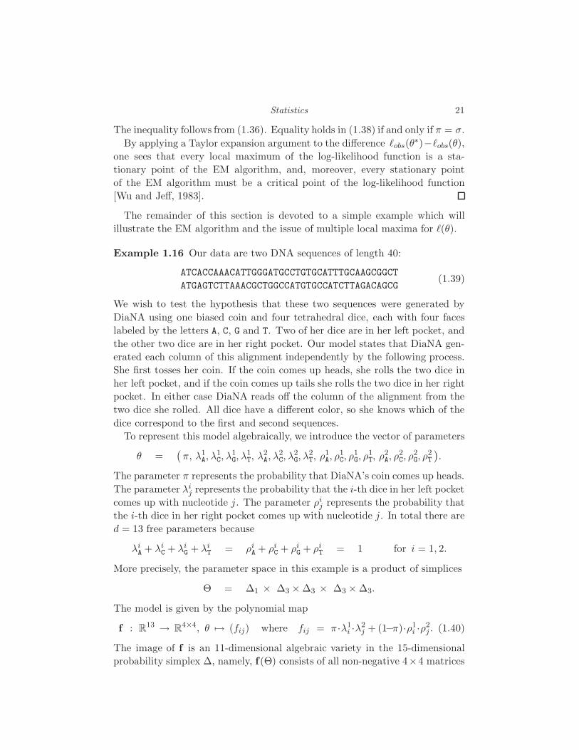
Example 1.16 Our data are two DNA sequences of length 40:
ATCACCAAACATTGGGATGCCTGTGCATTTGCAAGCGGCT
ATGAGTCTTAAACGCTGGCCATGTGCCATCTTAGACAGCG(1.39)
We wish to test the hypothesis that these two sequences were generated by
DiaNA using one biased coin and four tetrahedral dice, each with four faces
labeled by the letters A, C, G and T. Two of her dice are in her left pocket, and
the other two dice are in her right pocket. Our model states that DiaNA gen-
erated each column of this alignment independently by the following process.
She first tosses her coin. If the coin comes up heads, she rolls the two dice in
her left pocket, and if the coin comes up tails she rolls the two dice in her right
pocket. In either case DiaNA reads off the column of the alignment from the
two dice she rolled. All dice have a different color, so she knows which of the
dice correspond to the first and second sequences.
To represent this model algebraically, we introduce the vector of parameters
θ =(π, λ1
A, λ1C, λ
1G, λ
1T, λ
2A, λ
2C, λ
2G, λ
2T, ρ
1A, ρ
1C, ρ
1G, ρ
1T, ρ
2A, ρ
2C, ρ
2G, ρ
2T
).
The parameter π represents the probability that DiaNA’s coin comes up heads.
The parameter λij represents the probability that the i-th dice in her left pocket
comes up with nucleotide j. The parameter ρij represents the probability that
the i-th dice in her right pocket comes up with nucleotide j. In total there are
d = 13 free parameters because
λiA + λi
C + λiG + λi
T = ρiA + ρi
C + ρiG + ρi
T = 1 for i = 1, 2.
More precisely, the parameter space in this example is a product of simplices
Θ = ∆1 × ∆3 × ∆3 × ∆3 × ∆3.
The model is given by the polynomial map
f : R13 → R4×4, θ 7→ (fij) where fij = π ·λ1i ·λ2
j + (1−π)·ρ1i ·ρ2
j . (1.40)
The image of f is an 11-dimensional algebraic variety in the 15-dimensional
probability simplex ∆, namely, f(Θ) consists of all non-negative 4×4 matrices
22 L. Pachter and B. Sturmfels
of rank at most two having coordinate sum 1. The difference in dimensions
(11 versus 13) means that this model is non-identifiable: the preimage f−1(v)
of a rank 2 matrix v ∈ f(Θ) is a surface in the parameters space Θ.
Now consider the given alignment (1.39). Each pair of distinct nucleotides
occurs in precisely two columns. For instance, the pair CG occurs in the third
and fifth columns of (1.39). Each of the four identical pairs of nucleotides
(namely AA, CC, GG and TT) occurs in precisely four columns of the alignment.
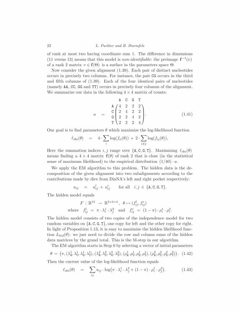
We summarize our data in the following 4 × 4 matrix of counts:
u =
A C G T
A 4 2 2 2
C 2 4 2 2
G 2 2 4 2
T 2 2 2 4
. (1.41)
Our goal is to find parameters θ which maximize the log-likelihood function
ℓobs(θ) = 4 ·∑
i
log(fii(θ)) + 2 ·∑
i6=j
log(fij(θ)),
Here the summation indices i, j range over A, C, G, T. Maximizing ℓobs(θ)
means finding a 4 × 4 matrix f(θ) of rank 2 that is close (in the statistical
sense of maximum likelihood) to the empirical distribution (1/40) · u.We apply the EM algorithm to this problem. The hidden data is the de-
composition of the given alignment into two subalignments according to the
contributions made by dice from DiaNA’s left and right pocket respectively:
uij = ulij + ur
ij for all i, j ∈ A, C, G, T.The hidden model equals
F : R13 → R2×4×4 , θ 7→ (f lij, f
rij)
where f lij = π · λ1
i · λ2j and fr
ij = (1− π) · ρ1i · ρ2
i .
The hidden model consists of two copies of the independence model for two
random variables on A, C, G, T, one copy for left and the other copy for right.
In light of Proposition 1.13, it is easy to maximize the hidden likelihood func-
tion Lhid(θ): we just need to divide the row and column sums of the hidden
data matrices by the grand total. This is the M-step in our algorithm.
The EM algorithm starts in Step 0 by selecting a vector of initial parameters
θ =(π, (λ1
A, λ1C, λ
1G, λ
1T), (λ
2A, λ
2C, λ
2G, λ
2T), (ρ
1A, ρ
1C, ρ
1G, ρ
1T), (ρ
2A, ρ
2C, ρ
2G, ρ
2T)). (1.42)
Then the current value of the log-likelihood function equals
ℓobs(θ) =∑
ij
uij · log(π · λ1
i · λ2j + (1− π) · ρ1
i · ρ2j
). (1.43)
Statistics 23
In the E-step we compute the expected hidden data by the following formulas:
ulij := uij ·
π · λ1i · λ2
j
π · λ1i · λ2
j + (1− π) · ρ1i · ρ2
j
for i, j ∈ A, C, G, T,
urij := uij ·
(1 − π) · ρ1i · ρ2
j
π · λ1i · λ2
j + (1− π) · ρ1i · ρ2
j
for i, j ∈ A, C, G, T.
In the subsequent M-step we now compute the maximum likelihood parameters
θ∗ =(π∗, λ1∗
A , λ1∗C , . . . , ρ
2∗T
)for the hidden model F . This is done by taking
row sums and column sums of the matrix (ulij) and the matrix (ur
ij), and by
defining the next parameters π to be the relative total counts of these two
matrices. In symbols, in the M-step we perform the following computations:
π∗ = 1N ·∑ij u
lij ,
λ1∗i = 1
N ·∑j ulij and ρ1∗
i = 1N ·∑j u
rij for i ∈ A, C, G, T,
λ2∗j = 1
N ·∑i ulij and ρ2∗
j = 1N ·∑i u
rij for j ∈ A, C, G, T.
Here N =∑
ij uij =∑
ij ulij +
∑ij u
rij is the sample size of the data.
After we are done with the M-step, the new value ℓobs(θ∗) of the likelihood
function is computed, using the formula (1.43). If ℓobs(θ∗) − ℓobs(θ) is small
enough then we stop and output the vector θ = θ∗ and the corresponding 4×4
matrix f(θ). Otherwise we set θ = θ∗ and return to the E-step.
Here are four numerical examples for the data (1.41) with sample size N =
40. In each of our experiments, the starting vector θ is indexed as in (1.42).
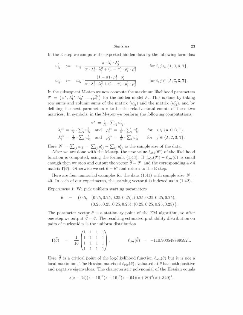
Experiment 1: We pick uniform starting parameters
θ =(0.5, (0.25, 0.25, 0.25, 0.25), (0.25, 0.25, 0.25, 0.25),
(0.25, 0.25, 0.25, 0.25), (0.25, 0.25, 0.25, 0.25)).
The parameter vector θ is a stationary point of the EM algorithm, so after
one step we output θ = θ. The resulting estimated probability distribution on
pairs of nucleotides is the uniform distribution
f(θ) =1
16
1 1 1 1
1 1 1 1
1 1 1 1
1 1 1 1
, ℓobs(θ) = −110.903548889592...
Here θ is a critical point of the log-likelihood function ℓobs(θ) but it is not a
local maximum. The Hessian matrix of ℓobs(θ) evaluated at θ has both positive
and negative eigenvalues. The characteristic polynomial of the Hessian equals
z(z − 64)(z − 16)2(z + 16)2(z + 64)(z + 80)4(z + 320)2.

24 L. Pachter and B. Sturmfels
Experiment 2: We decrease the starting parameter λ1A and we increase λ1
C:
θ =(0.5, (0.2, 0.3, 0.25, 0.25), (0.25, 0.25, 0.25, 0.25),
(0.25, 0.25, 0.25, 0.25), (0.25, 0.25, 0.25, 0.25)).
Now the EM algorithm converges to a distribution which is a local maximum:
f(θ) =1
54·
6 3 3 3
3 4 4 4
3 4 4 4
3 4 4 4
, ℓobs(θ) = −110.152332481077...
The Hessian of ℓobs(θ) at θ has rank 11, and all eleven non-zero eigenvalues are
distinct and negative.
Experiment 3: We next increase the starting parameter ρ1A and we decrease ρ1
C:
θ =(0.5, (0.2, 0.3, 0.25, 0.25), (0.25, 0.25, 0.25, 0.25),
(0.3, 0.2, 0.25, 0.25), (0.25, 0.25, 0.25, 0.25)).
The EM algorithm converges to a distribution which is a saddle point of ℓobs:
f(θ) =1
48·
4 2 3 3
2 4 3 3
3 3 3 3
3 3 3 3
, ℓobs(θ) = −110.223952742410...
The Hessian of ℓobs(θ) at θ has rank 11, with nine eigenvalues negative.
Experiment 4: Let us now try the following starting parameters:
θ =(0.5, (0.2, 0.3, 0.25, 0.25), (0.25, 0.2, 0.3, 0.25),
(0.25, 0.25, 0.25, 0.25), (0.25, 0.25, 0.25, 0.25)).
The EM algorithm converges to a probability distribution which is a local
maximum of the likelihood function, which is better than the local maximum
found previously in Experiment 2. The new winner is
f(θ) =1
40·
3 3 2 2
3 3 2 2
2 2 3 3
2 2 3 3
, ℓobs(θ) = −110.098128348563...
All 11 nonzero eigenvalues of the Hessian of ℓobs(θ) are distinct and negative.
We repeated this experiment many more times with random starting values,
and we never found a parameter vector that was better than the one found in
Statistics 25
Experiment 4. Based on this, we would like to conclude that the maximum
value of the observed likelihood function is attained by our best solution:
maxLobs(θ) : θ ∈ Θ
=
216 · 324
4040= e−110.0981283. (1.44)
Assuming that this conclusion is correct, let us discuss the set of all optimal
solutions. Since the data matrix u is invariant under the action of the symmet-
ric group on A, C, G, T, that group also acts on the set of optimal solutions.
There are three matrices like the one found in Experiment 4:
1
40·
3 3 2 2
3 3 2 2
2 2 3 3
2 2 3 3
,
1
40·
3 2 3 2
2 3 2 3
3 2 3 2
2 3 2 3
and
1
40·
3 2 2 3
2 3 3 2
2 3 3 2
3 2 2 3
. (1.45)
The preimage of each of these matrices under the polynomial map f is a surface
in the space of parameters θ, namely, it consists of all representations of a rank
2 matrix as a convex combination of two rank 1 matrices. The topology of
such “spaces of explanations” were studied in [Mond et al., 2003]. The finding
(1.44) indicates that the set of optimal solutions to the maximum likelihood
problem is the disjoint union of three “surfaces of explanations”.
But how do we know that (1.44) is actually true? Does running the EM
algorithm 100, 000 times without converging to a parameter vector whose like-
lihood is larger constitute a mathematical proof? Can it be turned into a
mathematical proof? Algebraic techniques for addressing such questions will
be introduced in Section 3.3. For a numerical approach see Chapter 20.
1.4 Markov models
We now introduce Markov chains, hidden Markov models and Markov models
on trees, using the algebraic notation of the previous sections. While our
presentation is self-contained, readers may find it useful to compare with the
(more standard) description of these models in [Durbin et al., 1998] or other
text books. A natural point of departure is the following toric model.
1.4.1 Toric Markov chains
We fix an alphabet Σ with l letters, and we fix a positive integer n. We shall
define a toric model whose state space is the set Σn of all words of length n.
The model is parameterized by the set Θ of non-negative l× l matrices. Thus
the number of parameters is d = l2 and the number of states is m = ln.
Every toric model with d parameters and m states is represented by a d×mmatrix A with integer entries as in Section 1.2. The d × m matrix which

26 L. Pachter and B. Sturmfels
represents the toric Markov model will be denoted by Al,n. Its rows are indexed
by Σ2 and its columns indexed by Σn. The entry of the matrix Al,n in the
row indexed by the pair σ1σ2 ∈ Σ2 and the column indexed by the word
π1π2 · · ·πn ∈ Σn is the number of occurrences of the pair inside the word, i.e.,
the number of indices i ∈ 1, . . . , n−1 such that σ1σ2 = πiπi+1. We define the
toric Markov chain model to be the toric model specified by the matrix Al,n.
For a concrete example let us consider words of length n = 4 over the binary
alphabet Σ = 0, 1, so that l = 2, d = 4 and m = 16. The matrix A2,4 which
was defined in the previous paragraph is the following 4 × 16 matrix:
0000 0001 0010 0011 0100 0101 0110 0111 1000 1001 1010 1011 1100 1101 1110 1111
00 3 2 1 1 1 0 0 0 2 1 0 0 1 0 0 0
01 0 1 1 1 1 2 1 1 0 1 1 1 0 1 0 0
10 0 0 1 0 1 1 1 0 1 1 2 1 1 1 1 0
11 0 0 0 1 0 0 1 2 0 0 0 1 1 1 2 3
.
We write R2×2 for the space of 2 × 2 matrices
θ =
(θ00 θ01
θ10 θ11
).
The parameter space Θ ⊂ R2×2 consists of all matrices θ whose four entries
θij are positive. The toric Markov chain model of length n = 4 for the binary
alphabet (l = 2) is the image of Θ = R2×2>0 under the monomial map
f2,4 : R2×2 → R16 , θ 7→ 1∑ijkl pijkl
· (p0000, p0001, . . . , p1111),
where pi1i2i3i4 = θi1i2 · θi2i3 · θi3i4 for all i1i2i3i4 ∈ 0, 14.
The map fl,n is defined analogously for larger alphabets and longer sequences.
The toric Markov chain model f2,4(Θ) is a three-dimensional object inside
the 15-dimensional simplex ∆ which consists of all probability distributions on
the state space 0, 14. Algebraically, the simplex is specified by the equation
p0000 + p0001 + p0010 + p0011 + · · ·+ p1110 + p1111 = 1. (1.46)
where the pijkl are unknowns which represent the probabilities of the 16 states.
To understand the geometry of the toric Markov chain model, we examine the
matrix A2,4. The 16 columns of A2,4 represent twelve distinct points in
(u00, u01, u10, u11) ∈ R2×2 : u00 + u01 + u10 + u11 = 3
≃ R3.
The convex hull of these twelve points is the three-dimensional polytope de-
picted in Figure 1.1. We refer to Section 2.3 for a general introduction to
polytopes. Only eight of the twelve points are vertices of the polytope.
Statistics 27
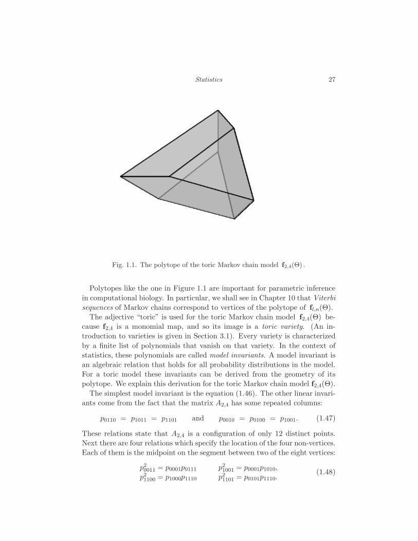
Fig. 1.1. The polytope of the toric Markov chain model f2,4(Θ) .
Polytopes like the one in Figure 1.1 are important for parametric inference
in computational biology. In particular, we shall see in Chapter 10 that Viterbi
sequences of Markov chains correspond to vertices of the polytope of fl,n(Θ).
The adjective “toric” is used for the toric Markov chain model f2,4(Θ) be-
cause f2,4 is a monomial map, and so its image is a toric variety. (An in-
troduction to varieties is given in Section 3.1). Every variety is characterized
by a finite list of polynomials that vanish on that variety. In the context of
statistics, these polynomials are called model invariants. A model invariant is
an algebraic relation that holds for all probability distributions in the model.
For a toric model these invariants can be derived from the geometry of its
polytope. We explain this derivation for the toric Markov chain model f2,4(Θ).
The simplest model invariant is the equation (1.46). The other linear invari-
ants come from the fact that the matrix A2,4 has some repeated columns:
p0110 = p1011 = p1101 and p0010 = p0100 = p1001. (1.47)
These relations state that A2,4 is a configuration of only 12 distinct points.
Next there are four relations which specify the location of the four non-vertices.
Each of them is the midpoint on the segment between two of the eight vertices:
p20011 = p0001p0111 p2
1001 = p0001p1010,
p21100 = p1000p1110 p2
1101 = p0101p1110.(1.48)
28 L. Pachter and B. Sturmfels
For instance, the first equation p20011 = p0001p0111 corresponds to the following
additive relation among the fourth, second and eighth column of A2,4:
2 · (1, 1, 0, 1) = (2, 1, 0, 0) + (0, 1, 0, 2).
The remaining eight columns of A2,4 are vertices of the polytope depicted
above. The corresponding probabilities satisfy the following relations:
p0111p1010 = p0101p1110 p0111p1000 = p0001p1110 p0101p1000 = p0001p1010,
p0111p21110 = p1010p
21111 p2
0111p1110 = p0101p21111 p0001p
21000 = p2
0000p1010,
p20000p0101 = p2
0001p1000 p20000p
31110 = p3
1000p21111 p2
0000p30111 = p3
0001p21111.
These nine equations together with (1.46), (1.47) and (1.48) characterize the set
of distributions p ∈ ∆ that lie in the toric Markov chain model f2,4(Θ). Tools
for computing such lists of model invariants will be presented in Chapter 3.
1.4.2 Markov Chains
The Markov chain model is a submodel of the toric Markov chain model. Let
Θ1 denote the subset of all matrices θ ∈ Rl×l>0 whose rows sum to one. The
Markov chain model is the image of Θ1 under the map fl,n. By a Markov
chain we mean any point p in the model fl,n(Θ1). This definition agrees with
the familiar description of Markov chains in [Durbin et al., 1998, Chapter 3],
except that we require the initial distribution at the first state to be uniform.
For instance, if l = 2 then the parameter space Θ1 is a square. Namely, Θ1
is the set of all pairs (θ0, θ1) ∈ R2 such that the following matrix is positive:
θ =
(θ0 1 − θ0
1 − θ1 θ1
)
The Markov chain model is the image of the square under the map f2,n. A
Markov chain of length n = 4 is any probability distribution of the form
p0000 =1
2θ30 , p0001 =
1
2θ20(1−θ0), p0010 = p1001 = p0100 =
1
2θ0(1−θ0)(1−θ1),
p0011 =1
2θ0(1 − θ0)θ1 , p0101 =
1
2(1− θ0)
2(1 − θ1) , p0111 =1
2(1− θ0)θ
21,
p0110 = p1011 = p1101 =1
2(1 − θ0)θ1(1− θ1) , p1010 =
1
2(1− θ1)
2(1 − θ0),
p1000 =1
2(1−θ1)θ20, p1100 =
1
2θ1(1−θ1)θ0, p1110 =
1
2θ21(1−θ1), p1111 =
1
2θ31.
Thus the Markov chain model is the surface in the 15-dimensional simplex ∆
given by this parameterization. It satisfies all the model invariants of the toric
Markov chain (a threefold in ∆) plus some extra model invariants due to the
Statistics 29
fact that probabilities must sum to 1, and the initial distribution is uniform.
For example,
p0000 + p0001 + p0010 + p0011 + p0100 + p0101 + p0110 + p0111 =1
2.
We next discuss maximum likelihood estimation for Markov chains. Fix a
data vector u ∈ Nln representing N observed sequences in Σn. The sufficient
statistic v = Al,n · u ∈ Nl2 is regarded as an l × l matrix. The entry vσ1i2
in row σ1 and column i2 of the matrix v equals the number of occurrences of
σ1i2 ∈ Σ2 as a consecutive pair in any of the N observed sequences.
Proposition 1.17 The maximum likelihood estimate of the data u ∈ Nln in
the Markov chain model is the l× l matrix θ =(θij)
in Θ1 with coordinates
θij =vij∑
s∈Σ viswhere v = Al,n · u.
Proof The likelihood function for the toric Markov chain model equals
L(θ) = θAl,n·u = θv =∏
ij∈Σ2
θvij
ij .
The log-likelihood function can be written as follows:
ℓ(θ) =∑
i∈Σ
(vi1 · log(θi1)+vi2 · log(θi2)+ · · ·+vi,l−1 · log(θi,l−1)+vil · log(θil)
).
The log-likelihood function for the Markov chain model is obtained by restrict-
ing this function to the set Θ1 of l × l matrices whose row sums are all equal
to one. Therefore, ℓ(θ) is the sum over all i ∈ Σ of the expressions
vi1 · log(θi1)+vi2 · log(θi2)+ · · ·+vi,l−1 · log(θi,l−1)+vil · log(1−l−1∑
s=1
θis). (1.49)
These expressions have disjoint sets of unknowns for different values of the
index i ∈ Σ. To maximize ℓ(θ) over Θ1, it hence suffices to maximize the
concave function (1.49) over the (l − 1)-dimensional simplex consisting of all
non-negative vectors (θi1, θi2, . . . , θi,l−1) of coordinate sum at most one. By
equating the partial derivatives of (1.49) to zero, we see that the unique critical
point has coordinates θij = vij/(vi1 + vi2 + · · ·+ vil) as desired.
We next introduce the fully observed Markov model that underlies the hidden
Markov model considered in Subsection 1.4.3. We fix the sequence length n
and we consider a first alphabet Σ with l letters and a second alphabet Σ′ with
l′ letters. The observable states in this model are pairs (σ, τ) ∈ Σn × (Σ′)n of
words of length n. A sequence of N observations in this model is summarized

30 L. Pachter and B. Sturmfels
in a matrix u ∈ Nln×(l′)nwhere u(σ,τ ) is the number of times the pair (σ, τ)
was observed. Hence, in this model, m = (l · l′)n.
The fully observed Markov model is parameterized by a pair of matrices
(θ, θ′) where θ is an l × l matrix and θ′ is an l × l′ matrix. The matrix θ
encodes a Markov chain as before: the entry θij represents the probability of
transitioning from state i ∈ Σ to j ∈ Σ. The matrix θ′ encodes the interplay
between the two alphabets: the entry θ′ij represents the probability of out-
putting symbol j ∈ Σ′ when the Markov chain is in state i ∈ Σ. As before in
the Markov chain model, we restrict ourselves to non-negative matrices whose
rows sum to one. To be precise, Θ1 now denotes the set of pairs of matrices
(θ, θ′) ∈ Rl×l>0 ×Rl×l′
>0 whose row sums are equal to one. Hence d = l(l+ l′+2).
The fully observed Markov model is the restriction to Θ1 of the toric model
F : Rd → Rm , (θ, θ′) 7→ p =(pσ,τ )
where pσ,τ =1
lθ′σ1τ1
θσ1σ2θ′σ2τ2
θσ2σ3θ′σ3τ3
θσ3σ4 · · ·θσn−1σnθ′σnτn
. (1.50)
The computation of maximum likelihood estimates for this model is an easy
extension of the method for Markov chains in Proposition 1.17. The role of
the matrix Al,n for Markov chains is now played by the following linear map
A : Nln×(l′)n → Nl×l ⊕ Nl×l′ .
The image of the basis vector eσ,τ corresponding to a single observation (σ, τ)
under A is the pair of matrices (w, w′), where wrs is the number of indices i
such that σiσi+1 = rs, and w′rt is the number of indices i such that σiτi = rt.
Let u ∈ Nln×(l′)nbe a matrix of data. The sufficient statistic is the pair
of matrices A · u = (v, v′). Here v ∈ Nl×l and v′ ∈ Nl×l′ . The likelihood
function Lhid : Θ1 → R of the fully observed Markov model is the monomial
Lhid(θ) = θv · (θ′)v′ .
Proposition 1.18 The maximum likelihood estimate for the data u ∈ Nln×(l′)n
in the fully observed Markov model is the matrix pair (θ, θ′) ∈ Θ1 with
θij =vij∑
s∈Σ visand θ′ij =
v′ij∑t∈Σ′ v′it
(1.51)
Proof This is entirely analogous to the proof of Proposition 1.17, the point
being that the log-likelihood function ℓhid(θ) decouples as a sum of expressions
like (1.49), each of which is easy to maximize over the relevant simplex.

Statistics 31
1.4.3 Hidden Markov Models
The hidden Markov model f is derived from the fully observed Markov model
F by summing out the first indices σ ∈ Σn. More precisely, consider the map
ρ : Rln×(l′)n −→ R(l′)n
obtained by taking the column sums of a matrix with ln rows and (l′)n columns.
The hidden Markov model is the algebraic statistical model defined by com-
posing the fully observed Markov model F with the marginalization map ρ:
f = ρ F : Θ1 ⊂ Rd −→ R(l′)n. (1.52)
Here, d = l(l+ l′ − 2) and it is natural to write Rd = Rl(l−1) × Rl(l′−1) since
the parameters are pairs of matrices (θ, θ′). We summarize:
Remark 1.19 The hidden Markov model is a polynomial map f from the
parameter space Rl(l−1) × Rl(l′−1) to the probability space R(l′)n. The degree
of f in the entries of θ is n − 1, and the degree of f in the entries of θ′ is n.
The notation in the definition in (1.52) is consistent with our discussion of
the Expectation Maximization (EM) algorithm in Section 1.3. Thus we can
find maximum likelihood estimates for the hidden Markov model by applying
the EM algorithm to f = ρ F .
Remark 1.20 The Baum-Welch algorithm is the special case of the EM al-
gorithm obtained by applying EM to the hidden Markov model f = ρ F .
The Baum-Welch algorithm in general, and Remark 1.20 in particular, are
discussed in Section 11.6 of [Durbin et al., 1998].
Example 1.21 Consider the occasionally dishonest casino which is featured
as running example in [Durbin et al., 1998]. In that casino they use a fair
die most of the time, but occasionally they switch to a loaded die. Our two
alphabets are Σ = fair, loaded and Σ′ = 1, 2, 3, 4, 5, 6 for the six possible
outcomes of rolling a die. Suppose a particular game involves rolling the dice
n = 4 times. This hidden Markov model has d = 12 parameters, appearing in
θ =
( fair loaded
fair x 1− x
loaded 1 − y y
)and
θ′ =
( 1 2 3 4 5 6
fair f1 f2 f3 f4 f5 1−∑5i=1 fi
loaded l1 l2 l3 l4 l5 1−∑5j=1 lj
).

32 L. Pachter and B. Sturmfels
Presumably, the fair die is really fair, so that f1 = f2 = f3 = f4 = f5 = 1/6,
but, to be on the safe side, let us here keep the fi as unknown parameters
This hidden Markov model (HMM) has m = 64 = 1, 296 possible outcomes,
namely, all the words τ = τ1τ2τ3τ4 in (Σ′)4. The coordinates of the map
f : R12 → R1296 in (1.52) are polynomials of degree 7 = 3 + 4:
pτ1τ2τ3τ4 =1
2·∑
σ1∈Σ
∑
σ2∈Σ
∑
σ3∈Σ
∑
σ4∈Σ
θ′σ1τ1θσ1σ2θ
′σ2τ2
θσ2σ3θ′σ3τ3
θσ3σ4θ′σ4τ4
.
Thus our HMM is specified by a list of 1, 296 polynomials pτ in the twelve
unknowns. The sum of all polynomials is 1. Each polynomial has degree three
in the two unknowns x, y and degree four in the ten unknowns f1, f2, . . . , l5.
Suppose we observe the game N times. These observations are our data.
The sufficient statistic is the vector (uτ ) ∈ N1296, where uτ = uτ1τ2τ3τ4 counts
the number of times the output sequence τ = τ1τ2τ3τ4 was observed. Hence∑τ∈(Σ′)4 uτ = N . The goal of EM is to maximize the log-likelihood function
ℓ(x, y, f1, . . . , f5, l1, . . . , l5
)=
∑
τ∈Σ′4
uτ1τ2τ3τ4 · log(pτ1τ2τ3τ4),
where (x, y) ranges over a square, (f1, . . . , f5) runs over a 5-simplex, and so
does (l1, . . . , l5). Our parameter space Θ1 ⊂ R12 is the product of the square
and the two 5-simplices. The Baum-Welch algorithm (i.e., the EM algorithm
for the HMM) aims to maximize ℓ over the 12-dimensional polytope Θ1.
1.4.4 Tree Models
Markov chains and hidden Markov models are special instances of tree models,
a class of models which we discuss next. We begin by defining the fully observed
tree model, from which we then derive the hidden tree model. These models
relate to each other in the same way that the hidden Markov model is the
composition of the fully observed Markov model with a marginalization map.
Let T be a rooted tree with n leaves. We write N (T ) for the set of all nodes
of T . This set includes the root, which is denoted r, and the leaves, which
are indexed by [n] = 1, 2, . . . , n. The set E(T ) of edges of T is a subset
of N (T ) × N (T ). Every edge is directed away from the root r. We use the
abbreviation kl for edges (k, l) ∈ E(T ). Every node i ∈ N (T ) represents a
random variable which takes values in a finite alphabet Σi. Our tree models
are parameterized by a collection of matrices θkl, one for each edge kl ∈ E(T ).
The rows of the matrix θkl are indexed by Σk, and the columns are indexed by
Σl. As before, we restrict ourselves to non-negative matrices whose rows sum to
one. Let Θ1 denote the collection of tuples(θkl)kl∈E(T )
of such matrices. The
dimension of the parameter space Θ1 is therefore d =∑
kl∈E(T ) |Σk|(|Σl|−1).
Statistics 33
The fully observed tree model is the restriction to Θ1 of the monomial map
FT : Rd → Rm , θ =(θkl)kl∈E(T )
7→ p = (pσ)
pσ =1
|Σr|·∏
kl∈E(T )
θklσkσl
. (1.53)
Here m =∏
i∈N(T ) |Σi|. The state space of this model is the Cartesian product
of the sets Σi. A state is a vector σ =(σi)i∈N(T ) where σi ∈ Σi. The factor
1/|Σr| means that we are assuming the root distribution to be uniform.
The fully observed tree model FT is (the restriction to Θ1 of) a toric model.
There is an easy formula for computing maximum likelihood parameters in this
model. The formula and its derivation is similar to that in Proposition 1.18.
The hidden tree model fT is obtained from the fully observed tree model
FT by summing out the internal nodes of the tree. Hidden tree models are
therefore defined on a restricted state space corresponding only to leaves of
the tree. The state space of the hidden tree model is Σ1 × Σ2 × · · · × Σn, the
product of the alphabets associated with the leaves of T . The cardinality of the
state space is m′ = |Σ1|·|Σ2| · · · |Σn|. There is a natural linear marginalization
map ρT : Rm → Rm′which takes real-valued functions on
∏i∈N(T ) Σi to real-
valued functions on∏n
i=1 Σi. We have fT = ρT FT .
Proposition 1.22 The hidden tree model fT : Rd → Rm′is a multilinear
polynomial map. Each of its coordinates has total degree |E(T )|, but is linear
when regarded as a function of the entries of each matrix θkl separately.
The model fT described here is also known as the general Markov model on
the tree T , relative to the given alphabets Σi. The adjective “general” refers to
the fact that the matrices θkl are distinct and their entries obey no constraints
beyond non-negativity and rows summing to one. In most applications of tree
models, the parameters (θkl)kl∈E(T ) are specialized in some manner, either by
requiring that some matrices are identical or by specializing each individual
matrix θkl to have fewer than |Σk| · (|Σl| − 1) free parameters.
Example 1.23 The hidden Markov model is a (specialization of the) hidden
tree model, where the tree T is the caterpillar tree depicted in Figure 1.2.
In the HMM there are only two distinct alphabets: Σi = Σ for i ∈N (T )\[n] and Σi = Σ′ for i ∈ [n]. The matrices θkl are all square and
identical along the non-terminal edges of the tree. A second matrix is used for
all terminal edges.
Maximum likelihood estimation for the hidden tree model can be done with
the EM algorithm, as described in Section 1.3. Indeed, the hidden tree model

34 L. Pachter and B. Sturmfels
Fig. 1.2. Two views of the caterpillar tree.
is the composition fT = ρT FT of an easy toric model FT and the marginal-
ization map ρT , so Algorithm 1.14 is directly applicable to this situation.
Tree models used in phylogenetics have the same alphabet Σ on each edge,
but the transition matrices remain distinct and independent. The two alpha-
bets most commonly used are Σ = 0, 1 and Σ = A, C, G, T. We present one
example for each alphabet. In both cases, the tree T is the claw tree, which
has no internal nodes other than the root: N (T ) = 1, 2, . . . , n, r.
Example 1.24 Let Σ = 0, 1 and T the claw tree with n = 6 leaves. The
hidden tree model fT has d = 12 parameters. It has m = 64 states which
are indexed by binary strings i1i2i3i4i5i6 ∈ Σ6. The model fT (Θ1) is the
12-dimensional variety in the 63-simplex given by the parameterization
pi1i2i3i4i5i6 =1
2θr10i1θ
r20i2θ
r30i3θ
r40i4θ
r50i5θ
r60i6 +
1
2θr11i1θ
r21i2θ
r31i3θ
r41i4θ
r51i5θ
r61i6.
If the root distribution is unspecified then d = 13 and the parameterization is
pi1i2i3i4i5i6 = λθr10i1θr20i2
θr30i3θr40i4
θr50i5θr60i6
+ (1−λ)θr11i1θr21i2
θr31i3θr41i4
θr51i5θr61i6
. (1.54)
The algebraic geometry of Examples 1.24 and 1.25 is discussed in Section 3.2.
Example 1.25 Let Σ = A, C, G, T and let T be the claw tree with n = 3
leaves. The hidden tree model fT has m = 64 states which are the triples
ijk ∈ Σ3. Writing λ = (λA, λC, λG, λT) for the root distribution, we have
pijk = λAθr1Ai θ
r2Ajθ
r3Ak + λCθ
r1Ci θ
r2Cjθ
r3Ck + λGθ
r1Gi θ
r2Gjθ
r3Gk + λTθ
r1Ti θ
r2Tjθ
r3Tk. (1.55)
If λ is unspecified then this model has d = 12 + 12 + 12 + 3 = 39 parameters.
If the root distribution is uniform, i.e., λ = ( 14 ,
14 ,
14 ,
14 ), then d = 36 = 12 +
12 + 12. We note that the small Jukes-Cantor model in Example 1.7 is the
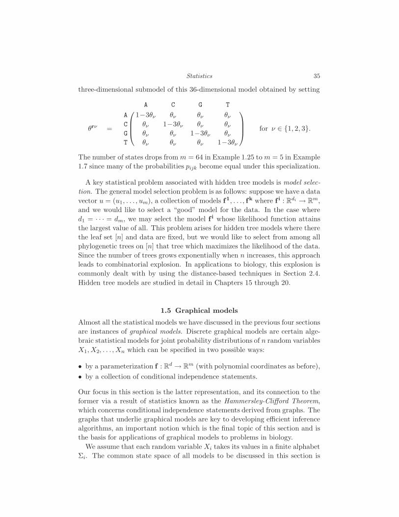
Statistics 35
three-dimensional submodel of this 36-dimensional model obtained by setting
θrν =
A C G T
A 1−3θν θν θν θνC θν 1−3θν θν θνG θν θν 1−3θν θνT θν θν θν 1−3θν
for ν ∈ 1, 2, 3.
The number of states drops fromm = 64 in Example 1.25 to m = 5 in Example
1.7 since many of the probabilities pijk become equal under this specialization.
A key statistical problem associated with hidden tree models is model selec-
tion. The general model selection problem is as follows: suppose we have a data
vector u = (u1, . . . , um), a collection of models f1, . . . , fk where f i : Rdi → Rm,
and we would like to select a “good” model for the data. In the case where
d1 = · · · = dm, we may select the model f i whose likelihood function attains
the largest value of all. This problem arises for hidden tree models where there
the leaf set [n] and data are fixed, but we would like to select from among all
phylogenetic trees on [n] that tree which maximizes the likelihood of the data.
Since the number of trees grows exponentially when n increases, this approach
leads to combinatorial explosion. In applications to biology, this explosion is
commonly dealt with by using the distance-based techniques in Section 2.4.
Hidden tree models are studied in detail in Chapters 15 through 20.
1.5 Graphical models
Almost all the statistical models we have discussed in the previous four sections
are instances of graphical models. Discrete graphical models are certain alge-
braic statistical models for joint probability distributions of n random variables
X1, X2, . . . , Xn which can be specified in two possible ways:
• by a parameterization f : Rd → Rm (with polynomial coordinates as before),
• by a collection of conditional independence statements.
Our focus in this section is the latter representation, and its connection to the
former via a result of statistics known as the Hammersley-Clifford Theorem,
which concerns conditional independence statements derived from graphs. The
graphs that underlie graphical models are key to developing efficient inference
algorithms, an important notion which is the final topic of this section and is
the basis for applications of graphical models to problems in biology.
We assume that each random variable Xi takes its values in a finite alphabet
Σi. The common state space of all models to be discussed in this section is
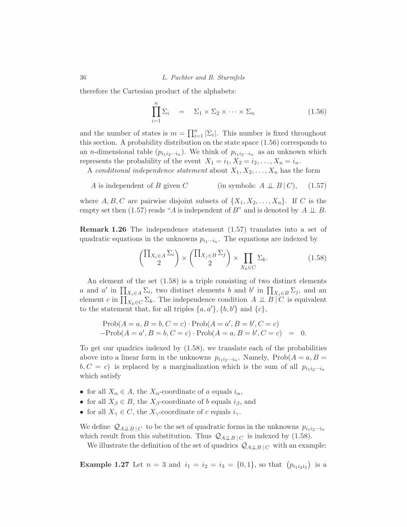
36 L. Pachter and B. Sturmfels
therefore the Cartesian product of the alphabets:
n∏
i=1
Σi = Σ1 × Σ2 × · · · × Σn (1.56)
and the number of states is m =∏n
i=1 |Σi|. This number is fixed throughout
this section. A probability distribution on the state space (1.56) corresponds to
an n-dimensional table (pi1i2···in). We think of pi1i2···in as an unknown which
represents the probability of the event X1 = i1, X2 = i2, . . . , Xn = in.
A conditional independence statement about X1, X2, . . . , Xn has the form
A is independent of B given C (in symbols: A ⊥⊥ B |C), (1.57)
where A,B, C are pairwise disjoint subsets of X1, X2, . . . , Xn. If C is the
empty set then (1.57) reads “A is independent of B” and is denoted by A ⊥⊥ B.
Remark 1.26 The independence statement (1.57) translates into a set of
quadratic equations in the unknowns pi1···in . The equations are indexed by(∏
Xi∈A Σi
2
)×(∏
Xj∈B Σj
2
)×∏
Xk∈C
Σk. (1.58)
An element of the set (1.58) is a triple consisting of two distinct elements
a and a′ in∏
Xi∈A Σi, two distinct elements b and b′ in∏
Xj∈B Σj, and an
element c in∏
Xk∈C Σk. The independence condition A ⊥⊥ B |C is equivalent
to the statement that, for all triples a, a′, b, b′ and c,
Prob(A = a, B = b, C = c) · Prob(A = a′, B = b′, C = c)
−Prob(A = a′, B = b, C = c) · Prob(A = a, B = b′, C = c) = 0.
To get our quadrics indexed by (1.58), we translate each of the probabilities
above into a linear form in the unknowns pi1i2···in . Namely, Prob(A = a, B =
b, C = c) is replaced by a marginalization which is the sum of all pi1i2···in
which satisfy
• for all Xα ∈ A, the Xα-coordinate of a equals iα,
• for all Xβ ∈ B, the Xβ-coordinate of b equals iβ , and
• for all Xγ ∈ C, the Xγ-coordinate of c equals iγ .
We define QA⊥⊥B |C to be the set of quadratic forms in the unknowns pi1i2···in
which result from this substitution. Thus QA⊥⊥B |C is indexed by (1.58).
We illustrate the definition of the set of quadrics QA⊥⊥B |C with an example:
Example 1.27 Let n = 3 and i1 = i2 = i3 = 0, 1, so that(pi1i2i3
)is a
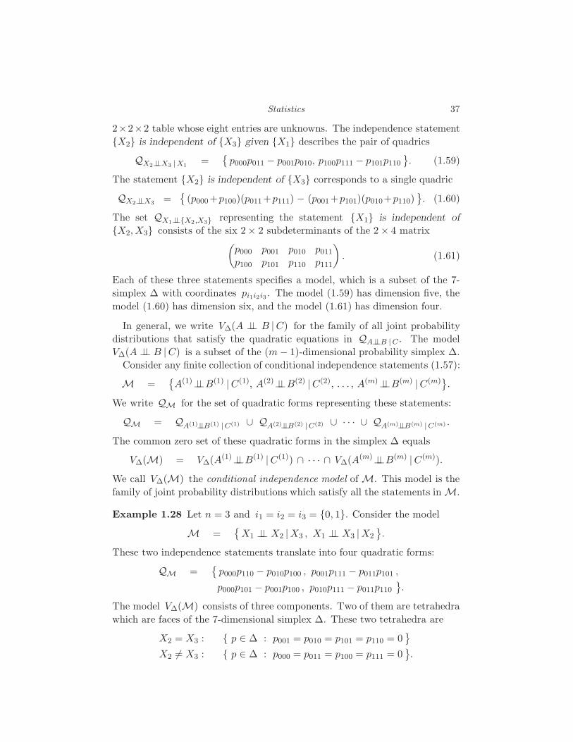
Statistics 37
2×2×2 table whose eight entries are unknowns. The independence statement
X2 is independent of X3 given X1 describes the pair of quadrics
QX2⊥⊥X3 |X1=
p000p011 − p001p010, p100p111 − p101p110
. (1.59)
The statement X2 is independent of X3 corresponds to a single quadric
QX2⊥⊥X3 =
(p000+p100)(p011+p111) − (p001+p101)(p010+p110). (1.60)
The set QX1⊥⊥X2,X3 representing the statement X1 is independent of
X2, X3 consists of the six 2× 2 subdeterminants of the 2 × 4 matrix(p000 p001 p010 p011
p100 p101 p110 p111
). (1.61)
Each of these three statements specifies a model, which is a subset of the 7-
simplex ∆ with coordinates pi1i2i3. The model (1.59) has dimension five, the
model (1.60) has dimension six, and the model (1.61) has dimension four.
In general, we write V∆(A ⊥⊥ B |C) for the family of all joint probability
distributions that satisfy the quadratic equations in QA⊥⊥B |C . The model
V∆(A ⊥⊥ B |C) is a subset of the (m− 1)-dimensional probability simplex ∆.
Consider any finite collection of conditional independence statements (1.57):
M =A(1)⊥⊥B(1) |C(1), A(2)⊥⊥B(2) |C(2), . . . , A(m)⊥⊥B(m) |C(m)
.
We write QM for the set of quadratic forms representing these statements:
QM = QA(1)⊥⊥B(1) |C(1) ∪ QA(2)⊥⊥B(2) |C(2) ∪ · · · ∪ QA(m)⊥⊥B(m) |C(m) .
The common zero set of these quadratic forms in the simplex ∆ equals
V∆(M) = V∆(A(1)⊥⊥B(1) |C(1)) ∩ · · · ∩ V∆(A(m)⊥⊥B(m) |C(m)).
We call V∆(M) the conditional independence model of M. This model is the
family of joint probability distributions which satisfy all the statements in M.
Example 1.28 Let n = 3 and i1 = i2 = i3 = 0, 1. Consider the model
M =X1 ⊥⊥ X2 |X3 , X1 ⊥⊥ X3 |X2
.
These two independence statements translate into four quadratic forms:
QM =p000p110 − p010p100 , p001p111 − p011p101 ,
p000p101 − p001p100 , p010p111 − p011p110
.
The model V∆(M) consists of three components. Two of them are tetrahedra
which are faces of the 7-dimensional simplex ∆. These two tetrahedra are
X2 = X3 : p ∈ ∆ : p001 = p010 = p101 = p110 = 0
X2 6= X3 : p ∈ ∆ : p000 = p011 = p100 = p111 = 0.
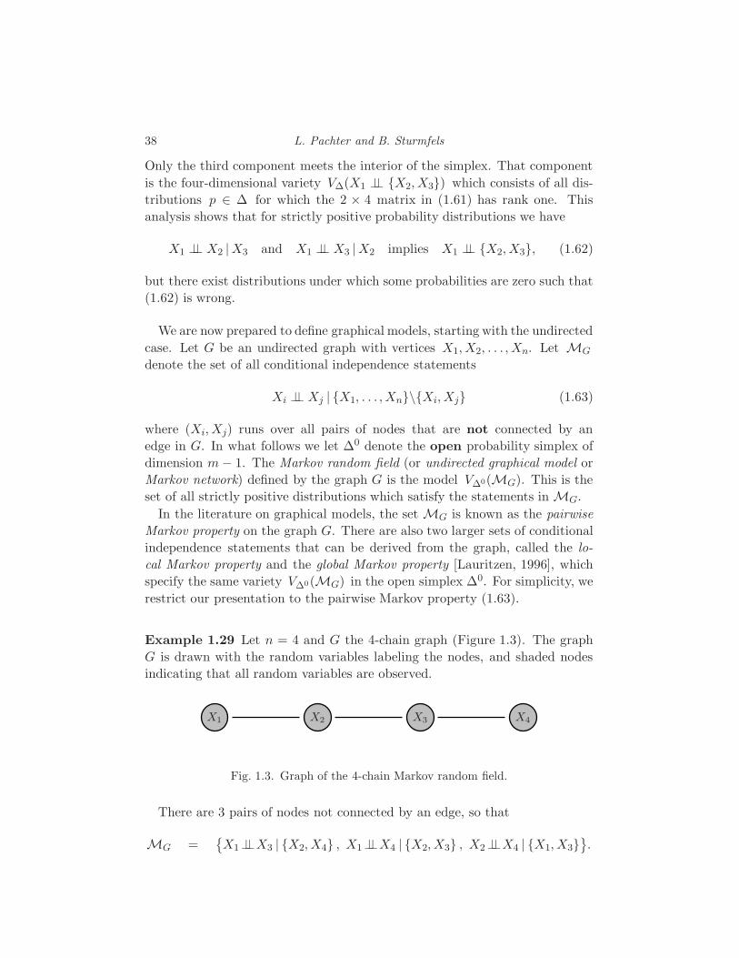
38 L. Pachter and B. Sturmfels
Only the third component meets the interior of the simplex. That component
is the four-dimensional variety V∆(X1 ⊥⊥ X2, X3) which consists of all dis-
tributions p ∈ ∆ for which the 2 × 4 matrix in (1.61) has rank one. This
analysis shows that for strictly positive probability distributions we have
X1 ⊥⊥ X2 |X3 and X1 ⊥⊥ X3 |X2 implies X1 ⊥⊥ X2, X3, (1.62)
but there exist distributions under which some probabilities are zero such that
(1.62) is wrong.
We are now prepared to define graphical models, starting with the undirected
case. Let G be an undirected graph with vertices X1, X2, . . . , Xn. Let MG
denote the set of all conditional independence statements
Xi ⊥⊥ Xj | X1, . . . , Xn\Xi, Xj (1.63)
where (Xi, Xj) runs over all pairs of nodes that are not connected by an
edge in G. In what follows we let ∆0 denote the open probability simplex of
dimension m− 1. The Markov random field (or undirected graphical model or
Markov network) defined by the graph G is the model V∆0(MG). This is the
set of all strictly positive distributions which satisfy the statements in MG.
In the literature on graphical models, the set MG is known as the pairwise
Markov property on the graph G. There are also two larger sets of conditional
independence statements that can be derived from the graph, called the lo-
cal Markov property and the global Markov property [Lauritzen, 1996], which
specify the same variety V∆0(MG) in the open simplex ∆0. For simplicity, we
restrict our presentation to the pairwise Markov property (1.63).
Example 1.29 Let n = 4 and G the 4-chain graph (Figure 1.3). The graph
G is drawn with the random variables labeling the nodes, and shaded nodes
indicating that all random variables are observed.
X1 X2 X3 X4
Fig. 1.3. Graph of the 4-chain Markov random field.
There are 3 pairs of nodes not connected by an edge, so that
MG =X1⊥⊥X3 | X2, X4 , X1⊥⊥X4 | X2, X3 , X2⊥⊥X4 | X1, X3
.

Statistics 39
For binary alphabets Σi the set QMGconsists of the twelve quadratic forms
p0010p1000 − p0000p1010 , p0001p1000 − p0000p1001 , p0001p0100 − p0000p0101 ,
p0011p1001 − p0001p1011 , p0011p1010 − p0010p1011 , p0011p0110 − p0010p0111 ,
p0110p1100 − p0100p1110 , p0101p1100 − p0100p1101 , p1001p1100 − p1000p1101 ,
p0111p1101 − p0101p1111 , p0111p1110 − p0110p1111 , p1011p1110 − p1010p1111.
Every Markov random field V∆0(MG) is, in fact, a toric model specified
parametrically by a matrix AG with entries in 0, 1. The columns of the
matrix AG are indexed by∏n
i=1 Σi. The rows are indexed by all the possible
assignments to the maximal cliques in G. A clique in G is a collection of nodes
any of two of which are connected by an edge. If the graph G contains no
triangles (as in Example 1.29 then the maximal cliques are just the edges.
An entry in the matrix AG is 1 if the states corresponding to the column
agree with the assignments specified by the row and is 0 otherwise. Returning
to Example 1.29, the matrix AG has 16 columns, and 12 rows. The rows are
indexed by tuples (i, j, σi, σj) where Xi, Xj is an edge of the graph G and
σi ∈ Σi and σj ∈ Σj. The nonzero entries of AG are therefore given by rows
(i, j, σi, σj) and columns π1π2 · · ·πn where σi = πi and σj = πj:
0000 0001 0010 0011 0100 0101 0110 0111 1000 1001 1010 1011 1100 1101 1110 1111
00 · · 1 1 1 1 0 0 0 0 0 0 0 0 0 0 0 0
01 · · 0 0 0 0 1 1 1 1 0 0 0 0 0 0 0 0
10 · · 0 0 0 0 0 0 0 0 1 1 1 1 0 0 0 0
11 · · 0 0 0 0 0 0 0 0 0 0 0 0 1 1 1 1
· 00 · 1 1 0 0 0 0 0 0 1 1 0 0 0 0 0 0
· 01 · 0 0 1 1 0 0 0 0 0 0 1 1 0 0 0 0
· 10 · 0 0 0 0 1 1 0 0 0 0 0 0 1 1 0 0
· 11 · 0 0 0 0 0 0 1 1 0 0 0 0 0 0 1 1
· · 00 1 0 0 0 1 0 0 0 1 0 0 0 1 0 0 0
· · 01 0 1 0 0 0 1 0 0 0 1 0 0 0 1 0 0
· · 10 0 0 1 0 0 0 1 0 0 0 1 0 0 0 1 0
· · 11 0 0 0 1 0 0 0 1 0 0 0 1 0 0 0 1
Each of the 12 rows corresponds to pairs in i1 × i2 or i2 × i3 or i3 × i4. For
instance, the label · 12 · of the sixth row represents (i, j, σi, σj) = (2, 3, 1, 2).
We note that each of the twelve quadrics in Example 1.29 corresponds to a
vector in the kernel of the matrix AG. For instance, the quadric p0010p1000 −p0000p1010 corresponds to the following vector in the kernel of AG:
(0000 0001 0010 0011 0100 0101 0110 0111 1000 1001 1010 1011 1100 1101 1110 1111
−1 0 1 0 0 0 0 0 1 0 −1 0 0 0 0 0)

40 L. Pachter and B. Sturmfels
The relationship between MG and the matrix AG generalizes as follows:
Theorem 1.30 (Undirected Hammersley-Clifford) The Markov random
field V∆0(MG) coincides with the toric model specified by the matrix AG.
Proof See [Lauritzen, 1996] and [Geiger et al., 2005].
Markov random fields are toric because their defining conditional indepen-
dence statements A ⊥⊥ B |C have the property that
A ∪ B ∪ C = X1, X2, . . . , Xn. (1.64)
This property ensures that all the quadrics in QA⊥⊥B |C are differences of two
monomials of the form p···p··· − p···p···. If the property (1.64) does not hold,
then the quadrics have more terms and the models are generally not toric.
Remark 1.31 It is important to note that the conditional independence state-
ments for a Markov random field are based on pairs of random variables not
joined by an edge in the graph. This should be contrasted with the parameters
in the toric model, where there are sets of parameters for each maximal clique
in the graph. The toric model parameters do not, in general, have an interpre-
tation as conditional probabilities. They are sometimes called potentials.
We now define directed graphical models which are generally not toric. We
also return to the closed simplex ∆. Let D be an acyclic directed graph with
nodes X1, X2, . . . , Xn. For any nodes Xi, let pa(Xi) denote the set of parents
of Xi in D and let nd(Xi) denote the set of non-descendants of Xi in D which
are not parents of Xi. The directed graphical model of D is described by the
following set of independence statements:
MD =Xi ⊥⊥ nd(Xi) | pa(Xi) : i = 1, 2, . . . , n
.
The directed graphical model V∆(MD) admits a polynomial parameterization,
which amounts to a directed version of the Hammersley-Clifford theorem. Be-
fore stating this parameterization in general, we first discuss a small example.
Example 1.32 LetD be the directed graph with nodes 1, 2, 3, 4 and four edges
(1, 2), (1, 3), (2, 4), (3, 4). Then MD =X2 ⊥⊥X3 |X1 , X4 ⊥⊥X1 | X2, X3
.
The quadrics associated with this directed graphical model are
QMD=
(p0000 + p0001)(p0110 + p0111) − (p0010 + p0011)(p0100 + p0101),
(p1000 + p1001)(p1110 + p1111)− (p1010 + p1011)(p1100 + p1101),
p0000p1001 − p0001p1000 , p0010p1011 − p0011p1010,
p0100p1101 − p0101p1100 , p0110p1111 − p0111p1110
.
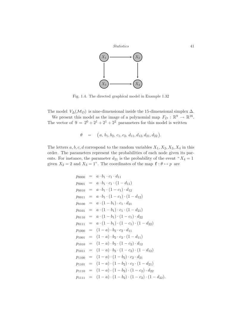
Statistics 41
X1 X2
X3 X4
Fig. 1.4. The directed graphical model in Example 1.32
The model V∆(MD) is nine-dimensional inside the 15-dimensional simplex ∆.
We present this model as the image of a polynomial map FD : R9 → R16.
The vector of 9 = 20 + 21 + 21 + 22 parameters for this model is written
θ =(a, b1, b2, c1, c2, d11, d12, d21, d22
).
The letters a, b, c, d correspond to the random variables X1, X2, X3, X4 in this
order. The parameters represent the probabilities of each node given its par-
ents. For instance, the parameter d21 is the probability of the event “X4 = 1
given X2 = 2 and X3 = 1”. The coordinates of the map f : θ 7→ p are
p0000 = a · b1 · c1 · d11
p0001 = a · b1 · c1 · (1− d11)
p0010 = a · b1 · (1− c1) · d12
p0011 = a · b1 · (1− c1) · (1 − d12)
p0100 = a · (1 − b1) · c1 · d21
p0101 = a · (1 − b1) · c1 · (1 − d21)
p0110 = a · (1 − b1) · (1 − c1) · d22
p0111 = a · (1 − b1) · (1 − c1) · (1 − d22)
p1000 = (1− a) · b2 · c2 · d11
p1001 = (1− a) · b2 · c2 · (1 − d11)
p1010 = (1− a) · b2 · (1 − c2) · d12
p1011 = (1− a) · b2 · (1 − c2) · (1 − d12)
p1100 = (1− a) · (1 − b2) · c2 · d21
p1101 = (1− a) · (1 − b2) · c2 · (1 − d21)
p1110 = (1− a) · (1 − b2) · (1− c2) · d22
p1111 = (1− a) · (1 − b2) · (1− c2) · (1− d22).

42 L. Pachter and B. Sturmfels
Note that the six quadrics in QMDare zero for these expressions, and also
2∑
i=1
2∑
j=1
2∑
k=1
2∑
l=1
pijkl = 1.
Let us return to our general discussion, where D is an acyclic directed graph
on n nodes, each associated with a finite alphabet Σi. It is known that the
dimension of the directed graphical model V∆(MD) equals
d =
n∑
i=1
(|Σi| − 1) ·∏
j∈pa(Xi)
|Σj|. (1.65)
We introduce a parameter θ(ν,π) for each element (ν, σ) ∈ Σi × ∏j∈pa(i) Σj,
where i ranges over all nodes. Thus the total number of parameters is d. These
parameters are supposed to satisfy the linear equations∑
ν∈Σi
θ(ν,π) = 1 for all σ ∈∏
j∈pa(Xi)
Σj. (1.66)
Thus the number of free parameters is equal to the right hand side of (1.65).
With the directed acyclic graph D we associate the following monomial map:
FD : Rd → Rm , θ 7→ p
where pσ =∏n
i=1 θ(σi,σ|pa(Xi)) for all σ ∈∏n
i=1 Σi
Here σ|pa(Xi) denotes the restriction of the vector σ to∏
j∈pa(Xi)Σj. Let Θ1
be the set of non-negative parameter vectors θ ∈ Rd which satisfy (1.66). The
following theorem generalizes the result derived for the graph in Example 1.32.
Theorem 1.33 (Directed Hammersley-Clifford) The directed graphical
model V∆(MD) equals the image of the parameter space Θ1 under the map FD.
Proof See Theorem 3.27 in [Lauritzen, 1996] and Theorem 3 in [Garcia et al., 2004].
Remark 1.34 Suppose that D = T is a rooted tree with all edges directed
away from the root r. The directed graphical model V∆(MD) is precisely
the fully observed tree model, and the parameterization FD specializes to the
parameterization given in (1.53). It is known that the model V∆(MT ) does
not depend on the location of the root r, and, in fact, the model coincides with
the Markov random field V∆(MG), where G denotes the undirected tree.
The inference problem for graphical models is to compute∑
σ∈S
pσ, (1.67)

Statistics 43
where S ranges over certain subsets of∏n
i=1 Σi.
The evaluation of the sum in (1.67) may be performed using ordinary arith-
metic, or with the tropical semiring, using min instead of +, and + instead
of ×, and replacing pσ with the negative of its logarithm (see Section 2.1).
In the case where S =∏n
i=1 Σi, (1.67) is equivalent to computing the parti-
tion function. If S is not equal to the entire product of the alphabets, then
it often fixes some of the coordinates. Here the inference problem involves a
marginalization, which we think of as evaluating one coordinate polynomial of
the model. Both of these problems are important statistically and very rele-
vant for biological applications. For example, if some of the variables Xi of
a Markov random field or directed graphical model D are hidden, then this
gives rise to a marginalization map ρD and to a hidden model fD = ρD FD.
Evaluating one coordinate of the polynomial map fD, also known as maximum
a posteriori (MAP) inference , is therefore exactly the evaluation of a subsum
of the partition function. The case of trees (discussed in Remark 1.34) is of
particular interest in computational biology. More examples are discussed in
Chapter 2, and connections to biology are developed in Chapter 4.
Remark 1.35 If inference with a graphical model involves computing the par-
tition function tropically, then the model is referred to as discriminative. In
the case where a specific coordinate(s) are selected before summing (1.67), then
the model is generative. These terms are used in statistical learning theory.
Inference can be computationally nontrivial for two reasons. In order to
compute the partition function, the number of terms in the sum is equal to m
which can be very large since many applications of graphical models require
that the models have large numbers of random variables. One may easily
encounter n = 200 binary random variables, in which case
m = 1606938044258990275541962092341162602522202993782792835301376.
The success of graphical models has been due to the possibility of efficient
inference for many models of interest. The organizing principle is the general-
ized distributive law which gives a recursive decomposition of (1.67) according
to the graph underlying the model.
Rather than explaining the details of the generalized distributive law in
general, we illustrate its origins and application with the hidden Markov model:
Example 1.36 Recall that the hidden Markov model is a polynomial map
f from the parameter space Rl(l−1) × Rl(l′−1) to the probability space R(l′)n.
Consider the case n = 4. If we treat the hidden Markov model as a special case
of the tree model (compare Figure 1.5 with Figure 1.2), allowing for different
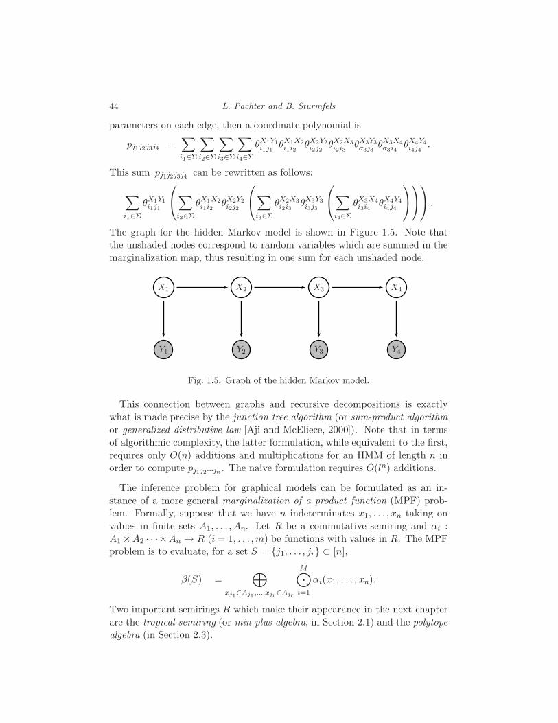
44 L. Pachter and B. Sturmfels
parameters on each edge, then a coordinate polynomial is
pj1j2j3j4 =∑
i1∈Σ
∑
i2∈Σ
∑
i3∈Σ
∑
i4∈Σ
θX1Y1i1j1
θX1X2i1i2
θX2Y2i2j2
θX2X3i2i3
θX3Y3σ3j3
θX3X4σ3i4
θX4Y4i4j4
.
This sum pj1j2j3j4 can be rewritten as follows:
∑
i1∈Σ
θX1Y1i1j1
∑
i2∈Σ
θX1X2i1i2
θX2Y2i2j2
∑
i3∈Σ
θX2X3i2i3
θX3Y3i3j3
∑
i4∈Σ
θX3X4i3i4
θX4Y4i4j4
.
The graph for the hidden Markov model is shown in Figure 1.5. Note that
the unshaded nodes correspond to random variables which are summed in the
marginalization map, thus resulting in one sum for each unshaded node.
X1 X2 X3 X4
Y1 Y2 Y3 Y4
Fig. 1.5. Graph of the hidden Markov model.
This connection between graphs and recursive decompositions is exactly
what is made precise by the junction tree algorithm (or sum-product algorithm
or generalized distributive law [Aji and McEliece, 2000]). Note that in terms
of algorithmic complexity, the latter formulation, while equivalent to the first,
requires only O(n) additions and multiplications for an HMM of length n in
order to compute pj1j2···jn . The naive formulation requires O(ln) additions.
The inference problem for graphical models can be formulated as an in-
stance of a more general marginalization of a product function (MPF) prob-
lem. Formally, suppose that we have n indeterminates x1, . . . , xn taking on
values in finite sets A1, . . . , An. Let R be a commutative semiring and αi :
A1 ×A2 · · ·×An → R (i = 1, . . . , m) be functions with values in R. The MPF
problem is to evaluate, for a set S = j1, . . . , jr ⊂ [n],
β(S) =⊕
xj1∈Aj1 ,...,xjr∈Ajr
M⊙
i=1
αi(x1, . . . , xn).
Two important semirings R which make their appearance in the next chapter
are the tropical semiring (or min-plus algebra, in Section 2.1) and the polytope
algebra (in Section 2.3).
2
Computation
Lior Pachter
Bernd Sturmfels
Many of the algorithms used for biological sequence analysis are discrete al-
gorithms, i.e., the key feature of the problems being solved is that some opti-
mization needs to be performed on a finite set. Discrete algorithms are comple-
mentary to numerical algorithms, such as Expectation Maximization, Singular
Value Decomposition and Interval Arithmetic, which make their appearance
in later chapters. They are also distinct from algebraic algorithms, such as the
Buchberger Algorithm, which is discussed in Section 3.1. In what follows we
introduce discrete algorithms and mathematical concepts which are relevant
for biological sequence analysis. The final section of this chapter offers an anno-
tated list of the computer programs which are used throughout the book. The
list ranges over all three themes (discrete, algebraic, numerical) and includes
software tools which are useful for research in computational biology.
Some discrete algorithms arise naturally from algebraic statistical models,
which are characterized by finitely many polynomials, each with finitely many
terms. Inference methods for drawing conclusions about missing or hidden
data depend on the combinatorial structure of the polynomials in the algebraic
representation of the models. In fact, many widely used dynamic programming
methods, such as the Needleman-Wunsch algorithm for sequence alignment,
can be interpreted as evaluating polynomials, albeit with tropical arithmetic.
The combinatorial structure of a polynomial, or polynomial map, is encoded
in its Newton polytope. Thus every algebraic statistical model has a Newton
polytope, and it is the structure of this polytope which governs dynamic pro-
gramming related to that model. Computing the entire polytope is what we
call parametric inference. This computation can be done efficiently in the poly-
tope algebra which is a natural generalization of tropical arithmetic. In Section
2.4 we study the combinatorics of one of the central objects in genome analysis,
phylogenetic trees, with an emphasis on the neighbor joining algorithm.
45

46 L. Pachter and B. Sturmfels
2.1 Tropical arithmetic and dynamic programming
Dynamic programming was introduced by Bellman in the 1950s to solve se-
quential decision problems with a compositional cost structure. Dynamic pro-
gramming offers efficient methods for progressively building a set of scores or
probabilities in order to solve a problem, and many discrete algorithms for bio-
logical sequence analysis are based on the principles of dynamic programming.
A convenient algebraic structure for stating various dynamic programming
algorithms is the tropical semiring (R ∪ ∞,⊕,⊙). The tropical semiring
consists of the real numbers R, together with an extra element ∞, and with
the arithmetic operations of addition and multiplication redefined as follows:
x ⊕ y := min(x, y) and x ⊙ y := x+ y.
In other words, the tropical sum of two real numbers is their minimum, and
the tropical product of two numbers is their sum. Here are some examples of
how to do arithmetic in this strange number system. The tropical sum of 3
and 7 is 3. The tropical product of 3 and 7 equals 10. We write this as follows:
3 ⊕ 7 = 3 and 3 ⊙ 7 = 10.
Many of the familiar axioms of arithmetic remain valid in the tropical semir-
ing. For instance, both addition and multiplication are commutative:
x ⊕ y = y ⊕ x and x ⊙ y = y ⊙ x.
The distributive law holds for tropical addition and tropical multiplication:
x ⊙ (y ⊕ z) = x ⊙ y ⊕ x⊙ z.
Both arithmetic operations have a neutral element. Infinity is the neutral
element for addition and zero is the neutral element for multiplication:
x ⊕ ∞ = x and x ⊙ 0 = x.
The tropical addition table and the tropical multiplication table look like this:
⊕ 1 2 3 4 5 6 7
1 1 1 1 1 1 1 1
2 1 2 2 2 2 2 2
3 1 2 3 3 3 3 3
4 1 2 3 4 4 4 4
5 1 2 3 4 5 5 5
6 1 2 3 4 5 6 6
7 1 2 3 4 5 6 7
⊙ 1 2 3 4 5 6 7
1 2 3 4 5 6 7 8
2 3 4 5 6 7 8 9
3 4 5 6 7 8 9 10
4 5 6 7 8 9 10 11
5 6 7 8 9 10 11 12
6 7 8 9 10 11 12 13
7 8 9 10 11 12 13 14
Although tropical addition and multiplication are straightforward, subtraction
Computation 47
is tricky. There is no tropical “10 minus 3” because the equation 3 ⊕ x = 10
has no solution x. In this book we use addition ⊕ and multiplication ⊙ only.
Example 2.1 It is important to keep in mind that 0 is the multiplicatively
neutral element. For instance, the tropical binomial coefficients are all 0, as in
(x⊕ y)3 = (x⊕ y)⊙ (x⊕ y) ⊙ (x⊕ y)
= 0 ⊙ x3 ⊕ 0 ⊙ x2y ⊕ 0 ⊙ xy2 ⊕ 0 ⊙ y3.
The zero coefficients can be dropped in this identity, and we conclude
(x⊕ y)3 = x3 ⊕ x2y ⊕ xy2 ⊕ y3 = x3 ⊕ y3.
This identity is known as Freshman’s dream and is verified by noting that
3 ·minx, y = min 3x, 2x+y, x+2y, 3y = min 3x, 3y holds for all real numbers x and y.
The familiar linear algebra operations of adding and multiplying vectors
and matrices make perfect sense over the tropical semiring. For instance, the
tropical scalar product in R3 of a row vector with a column vector is the scalar
(u1, u2, u3)⊙ (v1, v2, v3)T = u1 ⊙ v1 ⊕ u2 ⊙ v2 ⊕ u3 ⊙ v3
= minu1 + v1, u2 + v2, u3 + v3
.
Here is the product of a column vector and a row vector of length three:
(u1, u2, u3)T ⊙ (v1, v2, v3)
=
u1 ⊙ v1 u1 ⊙ v2 u1 ⊙ v3u2 ⊙ v1 u2 ⊙ v2 u2 ⊙ v3u3 ⊙ v1 u3 ⊙ v2 u3 ⊙ v3
=
u1 + v1 u1 + v2 u1 + v3u2 + v1 u2 + v2 u2 + v3u3 + v1 u3 + v2 u3 + v3
.
This 3 × 3 matrix is said to have tropical rank one.
To see why tropical arithmetic is relevant for discrete algorithms we consider
the problem of finding shortest paths in a weighted directed graph. This is a
standard problem of dynamic programming. Let G be a directed graph with n
nodes which are labeled by 1, 2, . . . , n. Every directed edge (i, j) in G has an
associated length dij which is a non-negative real number. If (i, j) is not an
edge of G then we set dij = +∞. We represent the weighted directed graph
G by its n × n adjacency matrix DG =(dij
)whose off-diagonal entries are
the edge lengths dij. The diagonal entries of DG are zero, i.e., dii = 0 for all i.
If G is an undirected graph with edge lengths, then we can represent G as a
directed graph with two directed edges (i, j) and (j, i) for each undirected edge
i, j. In that special case, DG is a symmetric matrix, and we can think of
dij = dji as the distance between node i and node j. For a general directed

48 L. Pachter and B. Sturmfels
graph G, the adjacency matrix DG will not be symmetric. Consider the result
of tropically multiplying the n × n matrix DG with itself n − 1 times:
D⊙n−1G = DG ⊙DG ⊙ · · · ⊙DG. (2.1)
This is an n× n matrix with entries in R≥0 ∪ +∞.
Proposition 2.2 Let G be a weighted directed graph on n nodes with n × n
adjacency matrix DG. Then the entry of the matrix D⊙n−1G in row i and column
j equals the length of a shortest path from node i to node j in G.
Proof Let d(r)ij denote the minimum length of any path from node i to node j
which uses at most r edges in G. Thus d(1)ij = dij for any two nodes i and j.
Since the edge weights dij were assumed to be non-negative, a shortest path
from node i to node j visits each node of G at most once. In particular, any
such shortest path in the directed graph G uses at most n − 1 directed edges.
Hence the length of a shortest path from i to j equals d(n−1)ij .
For r ≥ 2 we have the following recursive formula for these shortest paths:
d(r)ij = min
d
(r−1)ik + dkj : k = 1, 2, . . . , n
. (2.2)
Using tropical arithmetic, this formula can be rewritten as follows
d(r)ij = d
(r−1)i1 ⊙ d1j ⊕ d
(r−1)i2 ⊙ d2j ⊕ · · · ⊕ d
(r−1)in ⊙ dnj.
= (d(r−1)i1 , d
(r−1)i2 , . . . , d
(r−1)in ) ⊙ (d1j, d2j, . . . , dnj)
T .
From this it follows, by induction on r, that d(r)ij coincides with the entry in
row i and column j of the n × n matrix D⊙rG . Indeed, the right hand side of
the recursive formula is the tropical product of row i of D⊙r−1G and column j
of DG, which is the (i, j) entry of D⊙rG . In particular, d
(n−1)ij coincides with
the entry in row i and column j of D⊙n−1G . This proves the claim.
The iterative evaluation of the formula (2.2) is known as the Floyd-Warshall
Algorithm [Floyd, 1962, Warshall, 1962] for finding shortest paths in a weighted
digraph. Floyd-Warshall simply means performing the matrix multiplication
D⊙rG = D⊙r−1
G ⊙DG for r = 2, . . . , n− 1.
Example 2.3 Let G be the complete bi-directed graph on n = 4 nodes with
DG =
0 1 3 7
2 0 1 3
4 5 0 1
6 3 1 0
.

Computation 49
The first and second tropical power of this matrix are found to be
D⊙2G =
0 1 2 4
2 0 1 2
4 4 0 1
5 3 1 0
and D⊙3
G =
0 1 2 3
2 0 1 2
4 4 0 1
5 3 1 0
.
The entries in D⊙3G are the lengths of the shortest paths in the graph G.
The tropical computation above can be related to the following matrix com-
putation in ordinary arithmetic. Let ǫ denote an indeterminate, and let AG(ǫ)
be the n × n matrix whose entries are the monomials ǫdij . In our example,
AG(ǫ) =
1 ǫ1 ǫ3 ǫ7
ǫ2 1 ǫ1 ǫ3
ǫ4 ǫ5 1 ǫ1
ǫ6 ǫ3 ǫ1 1
.
Now compute the third power of this matrix in ordinary arithmetic
AG(ǫ)3 =
1 + 3ǫ3 + · · · 3ǫ+ ǫ4 + · · · 3ǫ2+3ǫ3+· · · ǫ3+6ǫ4 + · · ·3ǫ2 + 4ǫ5 + · · · 1 + 3ǫ3 + · · · 3ǫ+ ǫ3 + · · · 3ǫ2+3ǫ3+· · ·3ǫ4 + 2ǫ6 + · · · 3ǫ4+6ǫ5+· · · 1 + 3ǫ2 + · · · 3ǫ+ ǫ3 + · · ·6ǫ5 + 3ǫ6 + · · · 3ǫ3 + ǫ5 + · · · 3ǫ+ ǫ3 + · · · 1 + 3ǫ2 + · · ·
.
The entry of AG(ǫ)3 in row i and column j is a polynomial in ǫ which represents
the lengths of all paths from node i to node j using at most three edges. The
lowest exponent appearing in this polynomial is the (i, j)-entry in the matrix
D⊙3G . This is a general phenomenon, summarized informally as follows:
tropical = limǫ→0 log(classical(ǫ)
)(2.3)
This process of passing from classical arithmetic to tropical arithmetic is re-
ferred to as tropicalization. In the later sections of Chapter 3, we shall discuss
the tropicalization of algebraic-geometric objects such as curves and surfaces.
We shall give two more examples on how tropical arithmetic ties in natu-
rally with familiar algorithms in discrete mathematics. The first concerns the
dynamic programming approach to integer linear programming. The general
integer linear programming problem can be stated as follows. Let A = (aij)
be a d × n matrix of non-negative integers, let w = (w1, . . . , wn) be a row
vector with real entries, and let b = (b1, . . . , bd)T be a column vector with
non-negative integer entries. Our task is to find a non-negative integer column
vector u = (u1, . . . , un) which solves the following optimization problem:
Maximize w · u subject to u ∈ Nn and A · u = b. (2.4)
Let us further assume that all columns of the matrixA sum to the same number
50 L. Pachter and B. Sturmfels
α and that b1 + · · · + bd = m · α. This assumption is convenient because it
ensures that all feasible solutions u ∈ Nn of (2.4) satisfy u1 + · · ·+ un = m.
We can solve the integer programming problem (2.4) using tropical arith-
metic as follows. Let q1, . . . , qd be indeterminates and consider the expression
w1 ⊙ qa111 ⊙ qa21
2 ⊙ · · · ⊙ qad1d ⊕ · · · ⊕ wn ⊙ qa1n
1 ⊙ qa2n2 ⊙ · · · ⊙ qadn
d . (2.5)
Proposition 2.4 The optimal value of (2.4) is the coefficient of the monomial
qb11 q
b22 · · ·qbn
d in the m-th power, evaluated tropically, of the expression (2.5).
The proof of this proposition is not difficult and is similar to that of Propo-
sition 2.2. The process of taking the m-th power of the tropical polynomial
(2.5) can be regarded as solving the shortest path problem in a certain graph.
This is precisely the dynamic programming approach to integer linear program-
ming, as described in [Schrijver, 1986]. Prior to the result by [Lenstra, 1983]
that integer linear programming can be solved in polynomial time for fixed
dimensions, the dynamic programming method provided a polynomial-time
algorithm under the assumption that the integers in A are bounded.
Example 2.5 Let d = 2, n = 5 and consider the instance of (2.4) given by
A =
(4 3 2 1 0
0 1 2 3 4
), b =
(5
7
)and w = (2, 5, 11, 7, 3).
Here we have α = 4 and m = 3. The matrix A and the cost vector w are
encoded by a tropical polynomial as in (2.5):
f = 2q41 + 5q31q2 + 11q21q22 + 7q1q
32 + 3q42 .
The third power of this polynomial, evaluated tropically, is equal to
f ⊙ f ⊙ f = 6q121 + 9q11
1 q2 + 12q101 q
22 + 11q91q
32 + 7q81q
42 + 10q71q
52 + 13q61q
62
+12q51q72 + 8q41q
82 + 11q31q
92 + 17q21q
102 + 13q1q
112 + 9q12
2 .
The coefficient 12 of q51q72 in this tropical polynomial is the optimal value. An
optimal solution to this integer programming problem is u = (1, 1, 0, 0, 1)T.
Our final example concerns the notion of the determinant of an n×n matrix
Q = (qij). Since there is no negation in tropical arithmetic, the tropical deter-
minant is the same as the tropical permanent, namely, it is the sum over the
diagonal products obtained by taking all n! permutations π of 1, 2, . . . , n:
tropdet(Q) :=⊕
π∈Sn
q1π(1) ⊙ q2π(2) ⊙ · · · ⊙ qnπ(n). (2.6)
Here Sn denotes the symmetric group of permutations of 1, 2, . . . , n. The
evaluation of the tropical determinant is the classical assignment problem of
Computation 51
combinatorial optimization. Consider a company which has n jobs and n
workers, and each job needs to be assigned to exactly one of the workers. Let
qij be the cost of assigning job i to worker j. The company wishes to find the
cheapest assignment π ∈ Sn. The optimal total cost is the following minimum:
minq1π(1) + q2π(2) + · · ·+ qnπ(n) : π ∈ Sn
.
This number is precisely the tropical determinant of the matrix Q = (qij).
Remark 2.6 The tropical determinant solves the assignment problem.
In the assignment problem we need to find the minimum over n! quantities,
which appears to require exponentially many operations. However, there is a
well-known polynomial-time algorithm for solving this problem. The method
was introduced in [Kuhn, 1955] and is known as the Hungarian Assignment
Method. It maintains a price for each job and an (incomplete) assignment of
workers and jobs. At each iteration, the method chooses an unassigned worker
and computes a shortest augmenting path from this person to the set of jobs.
The total number of arithmetic operations is O(n3).
In classical arithmetic, the evaluation of determinants and the evaluation of
permanents are in different complexity classes. The determinant of an n × n
matrix can be computed in O(n3) steps, namely by Gaussian elimination,
while computing the permanent of an n× n matrix is a fundamentally harder
problem (it is #P -complete [Valiant, 1979]). It would be interesting to explore
whether the Hungarian Method can be derived from some version of Gaussian
Elimination by the principle of tropicalization (2.3).
To see what we mean, consider a 3 × 3 matrix A(ǫ) whose entries are poly-
nomials in the indeterminate ǫ. For each entry we list the term of lowest order:
A(ǫ) =
a11ǫ
q11 + · · · a12ǫq12 + · · · a13ǫ
q13 + · · ·a21ǫ
q21 + · · · a22ǫq22 + · · · a23ǫ
q23 + · · ·a31ǫ
q31 + · · · a32ǫq32 + · · · a33ǫ
q33 + · · ·
.
Suppose that the aij are sufficiently general non-zero real numbers, so that no
cancellation occurs in the lowest-order coefficient when we expand the deter-
minant of A(ǫ). Writing Q for the 3 × 3 matrix with entries qij, we have
det(A(ǫ)) = α · ǫtropdet(Q) + · · · for some α ∈ R\0.Thus the tropical determinant of Q can be extracted from this expression by
taking the logarithm and letting ǫ tend to zero, as suggested by (2.3).
The reader may have wondered where the adjective “tropical” comes from.
The algebraic structure (R∪ ∞,⊕,⊙), which is also known as the min-plus
algebra, has been invented (or re-invented) many times by many people. One
of its early developers, in the 1960s, was the Brazilian mathematician Imre

52 L. Pachter and B. Sturmfels
Simon. Simon’s work was followed up on by French scholars [Pin, 1998], who
coined the term “tropical semiring” for the min-plus algebra, in the honor
of their Brazilian colleague. Hence “tropical” stands for the French view of
Brazil. Currently, many mathematicians are working on tropical mathematics
and they are exploring a wide range of applications [Litvinov, 2005].
2.2 Sequence alignment
A fundamental task in computational biology is the alignment of DNA or pro-
tein sequences. Since biological sequences arising in practice are usually fairly
long, researchers have developed highly efficient algorithms for finding optimal
alignments. Although in some cases heuristics are used to reduce the combi-
natorial complexity, most of the algorithms are based on, or incorporate the
dynamic programming principle. An excellent introduction to the computer
science aspects of this subject is [Gusfield, 1997]. What we hope to accomplish
in this section is to explain what algebraic statistics and tropical arithmetic
have to do with discrete algorithms used for sequence alignment.
First, we give a self-contained explanation of the Needleman-Wunsch algo-
rithm for aligning biological sequences. Second, we explain a algebraic statis-
tical model for pairs of sequences, namely the pair hidden Markov model, and
we use Needleman-Wunsch to illustrate how dynamic programming algorithms
arise naturally from the tropicalization of this model.
We begin by specifying the sequence alignment problem in precise terms.
Fix a finite alphabet Σ with l letters, for instance, Σ = 0, 1, . . . , l − 1. If
l = 4 then the alphabet of choice is Σ = A, C, G, T. Suppose we are given
two sequences σ1 = σ11σ
12 · · ·σ1
n and σ2 = σ21σ
22 · · ·σ2
m over the alphabet Σ.
The sequence lengths n and m may be different. Our aim is to measure the
complexity of transforming the sequence σ1 into the sequence σ2 by changes
to individual characters, insertion of new characters, or deletion of existing
characters. Such changes are called edits. The sequence alignment problem is
to find the shortest sequence of edits that relates the two sequences σ1 and σ2.
Such sequences of edits are called alignments. The shortest sequence of edits
between σ1 and σ2 consists of at most n+m edits, and therefore it is a finite
problem to identify the best alignment: one can exhaustively enumerate all edit
sequences and then pick the shortest one. However, the exhaustive solution
can be improved on considerably. We shall present a dynamic programming
algorithm for solving the alignment problem which requires only O(nm) steps.
Each alignment of the pair (σ1, σ2) is represented by a string h over the edit
alphabet H, I, D. These letters stand for homology, insertion and deletion;
this terminology is explained in more detail in Chapter 4. We call the string h
the edit string of the alignment. An I in the edit string represents an insertion
Computation 53
in the first sequence σ1, a D in the edit string is a deletion in the first sequence
σ1, and an H is either a character change, or lack thereof. Writing #H,#I and
#D for the number of characters H, I and D in an edit string for an alignment
of the pair (σ1, σ2), we find that
#H + #D = n and #H + #I = m. (2.7)
Example 2.7 Let n = 7 andm = 9 and consider the sequences σ1 = ACGTAGC
and σ2 = ACCGAGACC. Then the following table shows an alignment of σ1 and
σ2 with #H = 6, #I = 3 and #D = 1. The first row is the edit string:
H H I H I H H I D H
A C − G − T A − G C
A C C G A G A C − C
(2.8)
Although the alignment has length ten, it represents the transformation of σ1
into σ2 by five edit steps which are performed from the left to the right. This
transformation is uniquely encoded by the edit string HHIHIHHIDH .
Proposition 2.8 A string over the edit alphabet H, I, D represents an align-
ment of an n-letter sequence σ1 and an m-letter sequence σ2 if and only if (2.7)
holds.
Proof As we perform the edits from the left to the right, every letter in σ1
either corresponds to a letter in σ2, in which case we record an H in the edit
string, or it gets deleted, in which case we record a D. This shows the first
identity in (2.7). The second identity holds because every letter σ2 either
corresponds to a letter in σ1, in which case there is an H in the edit string,
or it has been inserted, in which case we record an I in the edit string. Any
string over H, I, D with (2.7), when read from left to right, produces a valid
sequence of edits that transforms σ1 into σ2.
We write An,m for the set of all strings over H, I, D which satisfy (2.7).
We call An,m as the set of all alignments of the sequences σ1 and σ2, in spite
of the fact that it only depends on n and m rather than the specific sequences
σ1 and σ2. Each element h in An,m corresponds to a pair of sequences (µ1, µ2)
over the alphabet Σ ∪ − such that µ1 consists of a copy of σ1 together
with inserted “−” characters, and similarly µ2 is a copy of σ2 with inserted
“−” characters. The cardinalities of the sets An,m are the Delannoy numbers
[Stanley, 1999, §6.3]. They can be computed by a generating function.
Proposition 2.9 The cardinality of the set An,m of all alignments can be
computed as the coefficient of xmyn in the generating function 1/(1−x−y−xy).

54 L. Pachter and B. Sturmfels
Proof Consider the expansion of the given generating function
1
1 − x− y − xy=
∞∑
m=0
∞∑
n=0
am,nxmyn.
The coefficients are characterized by the linear recurrence
am,n = am−1,n +am,n−1+am−1,n−1 with a0,0 = 1, am,−1 = a−1,n = 0. (2.9)
The same recurrence is valid for the cardinality of An,m. Indeed, form+n ≥ 1,
every string in An,m is either a string in An−1,m−1 followed by an H , or a string
in An−1,m followed by an I , or it is a string in An,m−1 followed by a D. Also,
A0,0 has only one element, namely the empty string, and An,m is the empty
set if m < 0 or n < 0. Hence the numbers am,n and #An,m satisfy the same
initial conditions and the same recurrence (2.9), so they must be equal.
In light of the recurrence (2.9), it is natural to introduce the following graph.
Definition 2.10 The alignment graph Gn,m is the directed graph on the set
of nodes 0, 1, . . . , n × 0, 1, . . . , m and three classes of directed edges as
follows: there are edges labeled by I between pairs of nodes (i, j) → (i, j+1),
there are edges labeled by D between pairs of nodes (i, j) → (i + 1, j), and
there are edges labeled by H between pairs of nodes (i, j) → (i+ 1, j + 1).A C G T A G CA CCGAGA CCFig. 2.1. The alignment (2.8) shown as a path in the alignment graph G7,9.
Remark 2.11 The set An,m of all alignments is in bijection with the set of
paths from the node (0, 0) to the node (n,m) in the alignment graph Gn,m.

Computation 55
We have introduced three equivalent combinatorial objects: strings over
H, I, D satisfying (2.7), sequence pairs (µ1, µ2) that are equivalent to σ1, σ2
with the possible insertion of “−” characters, and paths in the alignment graph
Gn,m. All three represent alignments, and they are useful in designing algo-
rithms for finding good alignments. In order to formalize what “good” means,
we need to give scores to alignments. A scoring scheme is a pair of maps
w : Σ ∪ − × Σ ∪ − → R,
w′ : H, I, D × H, I, D → R.
Scoring schemes induce weights on alignments of sequences as follows. Fix
the two given sequences σ1 and σ2 over the alphabet Σ = A, C, G, T. Each
alignment is given by an edit string h over H, I, D. We write |h| for the
length of h. The edit string h determines the two sequences µ1 and µ2 of
length |h| over Σ ∪ −. The weight of the alignment h is defined to be
W (h) :=
|h|∑
i=1
w(µ1i , µ
2i ) +
|h|∑
i=2
w′(hi−1, hi). (2.10)
We represent a scoring scheme (w, w′) by a pair of matrices. The first one is
w =
wA,A wA,C wA,G wA,T wA,−
wC,A wC,C wC,G wC,T wC,−
wG,A wG,C wG,G wG,T wG,−
wT,A wT,C wT,G wT,T wT,−
w−,A w−,C w−,G w−,T
. (2.11)
Here the lower right entry w−,− is left blank because it is never used in com-
puting the weight of an alignment. The second matrix is a 3 × 3 matrix:
w′ =
w′H,H w′H,I w′H,D
w′I,H w′I,I w′I,D
w′D,H w′D,I w′D,D
(2.12)
Thus the total number of parameters in the alignment problem is 24+9 = 33.
We identify the space of parameters with R33. Each alignment h ∈ An,m of a
pair of sequences (σ1, σ2) gives rise to a linear functional W (h) on R33.
For instance, the weight of the alignment h = HHIHIHHIDH of our
sequences σ1 = ACGTAGC and σ2 = ACCGAGACC is the linear functional
W (h) = 2 · wA,A + 2 · wC,C +wG,G + wT,G + 2 ·w−,C +w−,A +wG,−
+ 2 · w′H,H + 3 · w′H,I + 2 · w′I,H + w′I,D + w′D,H .
Suppose we are given two input sequences σ1 and σ2 of lengths n and m
over the alphabet Σ. Suppose further that we are given a fixed scoring scheme

56 L. Pachter and B. Sturmfels
(w, w′). The global alignment problem is to compute an alignment h ∈ An,m
whose weight W (h) is minimal among all alignments in An,m. In the com-
putational biology literature, it is more common to use “maximal” instead of
“minimal”, but, of course, that is equivalent if we replace (w, w′) by (−w,−w′).In the following discussion let us simplify the problem and assume that
w′ = 0, so the weight of an alignment is the linear functional W (h) =∑|h|i=1 w(µ1
i , µ2i ) on R24. The problem instance (σ1, σ2, w) induces weights
on the edges of the alignment graph Gn,m as follows. The weight of the edge
(i, j) → (i + 1, j) is w(σ1i+1,−), the weight of the edge (i, j) → (i, j + 1) is
w(−, σ2j+1), and the weight of the edge (i, j) → (i+ 1, j + 1) is w(σ1
i+1, σ2j+1).
This gives a graph-theoretic reformulation of the global alignment problem.
Remark 2.12 The global alignment problem is equivalent to finding the min-
imum weight path from (0, 0) to (n,m) in the alignment graph Gn,m.
Thus the global alignment problem is equivalent to finding shortest paths in a
weighted graph. Proposition 2.2 gave general dynamic programming algorithm
for the shortest path problem, the Floyd-Warshall algorithm, which amounts to
multiplying matrices in tropical arithmetic. For the specific graph and weights
arising in the global alignment problem, this translates into an O(nm) dynamic
programming algorithm, called the Needleman-Wunsch algorithm.
Algorithm 2.13 (Needleman-Wunsch)
Input: Two sequences σ1 ∈ Σn, σ2 ∈ Σm and a scoring scheme w ∈ R24.
Output: An alignment h ∈ An,m whose weight W (h) is minimal.
Initialization: Create an (n+ 1)× (m+ 1) matrix M whose rows are indexed
by 0, 1, . . . , n and whose columns indexed by 0, 1, . . . , m. Set M [0, 0] = 0.
Set M [i, 0] := M [i− 1, 0] +w(σ1i ,−) for i = 1, . . . , n
and M [0, j] := M [0, j − 1] + w(−, σ2j ) for j = 1, . . . , m.
Loop: For i = 1, . . . , n and j = 1, . . . , m set
M [i, j] := min
M [i− 1, j − 1] + w(σ1i , σ
2j )
M [i− 1, j] + w(−, σ2j )
M [i, j − 1] + w(σ1i ,−)
Color one or more of the three edges which are adjacent to and directed towards
(i, j), and which attain the minimum.
Backtrack: Trace an optimal path from in backwards direction from (n,m) to
(0, 0). This is done by following an arbitrary sequence of colored edges.
Output: The edge labels in H, I, D of an optimal path in forward direction.
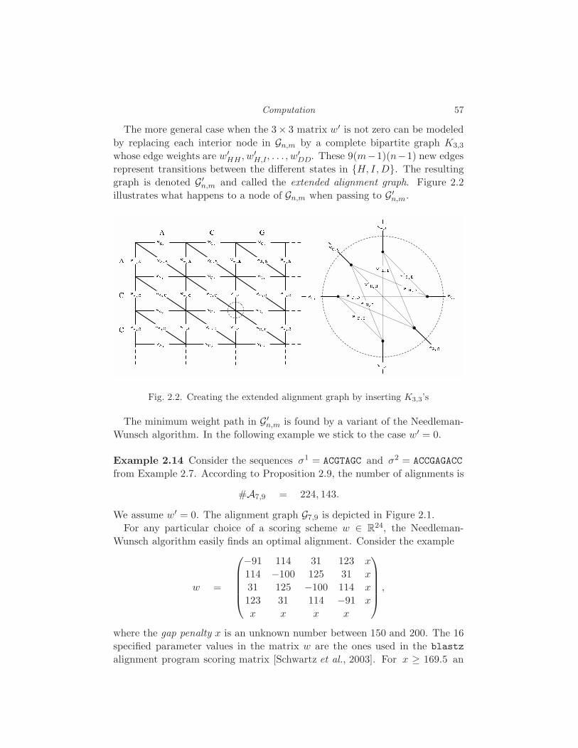
Computation 57
The more general case when the 3× 3 matrix w′ is not zero can be modeled
by replacing each interior node in Gn,m by a complete bipartite graph K3,3
whose edge weights are w′HH , w′H,I, . . . , w
′DD. These 9(m−1)(n−1) new edges
represent transitions between the different states in H, I, D. The resulting
graph is denoted G ′n,m and called the extended alignment graph. Figure 2.2
illustrates what happens to a node of Gn,m when passing to G ′n,m.
w ' H , Iw ' D , Iw , C
w ' H , H w ' I , Iw ' D , D w ' H , Dw ' I , Dw , C
w C , w G , w G , C
w C , Cw , Cw , Aw , C
w , Aw , Cw , Cw , Cw , Aw , Cw , C
w , Aw , Cw G , w C , w A , w A , w G , w C , w A , w C , w G , w C , w A , w G , w A , A w C , C w G , Cw A , C w C , Cw A , C w G , Cw C , A w G , AA C GACC
Fig. 2.2. Creating the extended alignment graph by inserting K3,3’s
The minimum weight path in G ′n,m is found by a variant of the Needleman-
Wunsch algorithm. In the following example we stick to the case w′ = 0.
Example 2.14 Consider the sequences σ1 = ACGTAGC and σ2 = ACCGAGACC
from Example 2.7. According to Proposition 2.9, the number of alignments is
#A7,9 = 224, 143.
We assume w′ = 0. The alignment graph G7,9 is depicted in Figure 2.1.
For any particular choice of a scoring scheme w ∈ R24, the Needleman-
Wunsch algorithm easily finds an optimal alignment. Consider the example
w =
−91 114 31 123 x
114 −100 125 31 x
31 125 −100 114 x
123 31 114 −91 x
x x x x
,
where the gap penalty x is an unknown number between 150 and 200. The 16
specified parameter values in the matrix w are the ones used in the blastz
alignment program scoring matrix [Schwartz et al., 2003]. For x ≥ 169.5 an
58 L. Pachter and B. Sturmfels
optimal alignment ish
µ1
µ2
=
H D H H D H H H H
A − C G − T A G C
A C C G A G A C C
with W (h) = 2x− 243.
If the gap penalty x is below 169.5 then an optimal alignment ish
µ1
µ2
=
H D H H I H H D D H
A − C G T A G − − C
A C C G − A G A C C
with W (h) = 4x− 582.
After verifying this computation, the reader may now wish to vary all 24 pa-
rameters in the matrix w and run the Needleman-Wunsch algorithm many
times. How does the resulting optimal alignment change? How many of the
224, 143 alignments occur for some choice of scoring scheme w? Is there a scor-
ing scheme w ∈ R24 which makes the alignment (2.8) optimal? Such questions
form the subject of parametric alignment [Gusfield et al., 1994, Gusfield, 1997]
which is the topic of Chapter 7.
We now shift gears and present the pair hidden Markov model for alignments.
This is an algebraic statistical model which depends on two integers n and m:
f : R33 → R4n+m. (2.13)
The 4n+m states are the pairs (σ1, σ2) of sequences of length n and m. The
33 = 24 + 9 parameters are written as a pair of matrices (θ, θ′) where
θ =
θA,A θA,C θA,G θA,T θA,−θC,A θC,C θC,G θC,T θC,−θG,A θG,C θG,G θG,T θG,−θT,A θT,C θT,G θT,T θT,−θ−,A θ−,C θ−,G θ−,T
, θ′ =
θ′H,H θ′H,I θ′H,D
θ′I,H θ′I,I θ′I,D
θ′D,H θ′D,I θ′D,D
(2.14)
In order to be statisticallymeaningful these parameters have to be non-negative
and satisfy six independent linear equations. Namely, they must lie in
Θ = ∆15 × ∆3 × ∆3 × ∆2 × ∆2 × ∆2 ⊂ R33.
The parameter space Θ is the product of six simplices of dimensions 15, 3, 3, 2, 2
and 2. The big simplex ∆15 consists of all non-negative 4×4 matrices (θij)i,j∈Σ
whose entries sum to 1. The two tetrahedra ∆3 come from requiring that
θ−,A + θ−,C + θ−,G + θ−,T = θA,− + θC,− + θG,− + θT,− = 1.
The three triangles ∆2 come from requiring that
θ′H,H + θ′H,I + θ′H,D = θ′I,H + θ′I,I + θ′I,D = θ′D,H + θ′D,I + θ′D,D = 1.

Computation 59
The coordinate fσ1,σ2 of the pair hidden Markov model f represents the
probability of observing the pair of sequences (σ1, σ2). This is the polynomial
fσ1,σ2 =∑
h∈An,m
|h|∏
i=1
θµ1i ,µ2
i·|h|∏
i=2
θ′hi−1,hi. (2.15)
Here (µ1, µ2) is the pair of sequences over Σ ∪ − which corresponds to h.
The following observation is crucial for understanding parametric alignment.
Proposition 2.15 The objective function of the sequence alignment problem
is the tropicalization of a coordinate polynomial fσ1,σ2 of the pair HMM.
Proof The tropicalization of the polynomial (2.15) is gotten by replacing the
outer sum by a tropical sum ⊕ and the inner products by tropical products
⊙. We replace each unknown θ... by the corresponding unknown w..., which we
think of as the negated logarithm of θ.... The result is the tropical polynomial
trop(fσ1,σ2) =⊕
h∈An,m
|h|⊙
i=1
wµ1i ,µ2
i·|h|⊙
i=2
w′hi−1,hi. (2.16)
The tropical product inside the tropical sum is precisely the weight W (h) of
the alignment h or (µ1, µ2) as defined in (2.10). Hence (2.16) is equivalent to
trop(fσ1,σ2) = minh∈An,mW (h).
Evaluating the right hand side of this expression is therefore equivalent to
finding an optimal alignment of the two sequences σ1 and σ2.
Remark 2.16 Since the logarithm of a probability is always negative, the
correspondence in Proposition 2.15 only accounts for scoring schemes in which
the weights have the same sign. Scoring schemes in which the weights have
mixed signs, as in Example 2.14, result from associating w... with the log-odds
ratio log(θ.../θ...) where the θ... are additional new parameters.
It is an instructive exercise to show that the sum of the polynomials fσ1,σ2
over all 4n+m pairs of sequences (σ1, σ2) simplifies to 1 when (θ, θ′) lies in Θ.
The key idea is to derive a recursive decomposition of the polynomial fσ1,σ2 by
grouping together all summands with fixed last factor pair θ′h|h|−1 ,h|h|θµ1
|h|,µ2
|h|.
This recursive decomposition is equivalent to performing dynamic program-
ming along the extended alignment graph G ′n,m. The variant of the Needleman-
Wunsch algorithm on the graph G ′n,m is precisely the efficient evaluation of the
tropical polynomial trop(fσ1,σ2) using the same recursive decomposition.

60 L. Pachter and B. Sturmfels
We explain this circle of ideas for the simpler case of Algorithm 2.13 where
w′ =
0 0 0
0 0 0
0 0 0
To be precise, we shall implement dynamic programming on the alignment
graph Gn,m as the efficient computation of a (tropical) polynomial. In term of
the pair HMM, this means that we are fixing all entries of the 3 × 3 matrix θ′
to be identical. Let us consider the following two possible specializations:
θ′ =
1/3 1/3 1/3
1/3 1/3 1/3
1/3 1/3 1/3
and θ′ =
1 1 1
1 1 1
1 1 1
The first specialization is the statistically meaningful one, but it leads to more
complicated formulas in the coefficients. For that reason we use the second
specialization in our implementation. We write gσ1,σ2 for the polynomial in
the 24 unknowns θ··· gotten from fσ1,σ2 by setting each of the 9 unknowns θ···to 1. The following short Maple code computes the polynomial gs1,s2 for
s1 := [A,C,G]: s2 := [A,C,C]:
T := array([ [ tAA, tAC, tAG, tAT, t_A ],
[ tCA, tCC, tCG, tCT, t_C ],
[ tGA, tGC, tGG, tGT, t_G ],
[ tTA, tTC, tTG, tTT, t_T ],
[ tA_, tC_, tG_, tT_, 0 ]]):
This represents the matrix θ with tAA = θAA, tAC = θAC, . . . etc. We initialize
n := nops(s1): m := nops(s2):
u1 := subs(A=1,C=2,G=3,T=4,s1):
u2 := subs(A=1,C=2,G=3,T=4,s2):
M := array([],0..n,0..m): M[0,0] := 1:
for i from 1 to n do
M[i,0] := M[i-1,0] * T[u1[i],5]:
od:
for j from 1 to m do
M[0,j] := M[0,j-1] * T[5,u2[j]]:
od:
We then perform a loop precisely as in Algorithm 2.13, with tropical arithmetic
on real numbers replaced by ordinary arithmetic on polynomials.
for i from 1 to n do
Computation 61
for j from 1 to m do
M[i,j] := M[i-1,j-1] * T[u1[i],u2[j]] + M[i-1, j ] *
T[u1[i], 5 ] + M[ i ,j-1] * T[ 5 ,u2[j]]:
od:
od:
lprint(M[n,m]);
Our Maple code produces a recursive decomposition of the polynomial gACG,ACC:
((tAA+2*tA_*t_A)*tCC+(tA_*tAC+tA_*tC_*t_A+(tAA+2*tA_*t_A)*tC_)
*t_C+(t_A*tCA+(tAA+2*tA_*t_A)*t_C+t_A*t_C*tA_)*tC_)*tGC+((tA_*
tAC+tA_*tC_*t_A+(tAA+2*tA_*t_A)*tC_)*tCC+(tA_*tC_*tAC+tA_*tC_^2
*t_A+(tA_*tAC+tA_*tC_*t_A+(tAA+2*tA_*t_A)*tC_)*tC_)*t_C+((tAA+
2*tA_*t_A)*tCC+(tA_*tAC+tA_*tC_*t_A+(tAA+2*tA_*t_A)*tC_)*t_C+
(t_A*tCA+(tAA+2*tA_*t_A)*t_C+t_A*t_C*tA_)*tC_)*tC_)*t_G+((t_A*
tCA+(tAA+2*tA_*t_A)*t_C+t_A*t_C*tA_)*tGC+((tAA+2*tA_*t_A)*tCC+
(tA_*tAC+tA_*tC_*t_A+(tAA+2*tA_*t_A)*tC_)*t_C+(t_A*tCA+(tAA+2*
tA_*t_A)*t_C+t_A*t_C*tA_)*tC_)*t_G+(t_A*t_C*tGA+(t_A*tCA+(tAA+
2*tA_*t_A)*t_C+t_A*t_C*tA_)*t_G+t_A*t_C*t_G*tA_)*tC_)*tC_
The expansion of this polynomial has 14 monomials. The sum of its coefficients
is #A3,3 = 63. Next we run same code for the sequences of Example 2.7:
s1 := [A,C,G,T,A,G,C]: s2 := [A,C,C,G,A,G,A,C,C]:
The expansion of the resulting polynomial gs1,s2 has 1, 615 monomials, and
the sum of its coefficients equals #A7,9 = 224, 143. Each monomial in gs1,s2represents a family of alignments h all of which have the same W (h). We have
chosen a simple example to illustrate the main points, but the method shown
can be used for computing the polynomials associated to much longer sequence
pairs. We summarize our discussion of sequence alignment as follows:
Remark 2.17 The Needleman-Wunsch algorithm is the tropicalization of the
pair hidden Markov model for sequence alignment.
In order to answer parametric questions, such as the ones raised at the end
of Example 2.14, we need to better understand the combinatorial structure
encoded in the polynomials fσ1,σ2 and gσ1,σ2 . The key to unraveling this com-
binatorial structure lies in the study of polytopes, which is the our next topic.
2.3 Polytopes
In this section we review basic facts about convex polytopes and algorithms for
computing them, and we explain how they relate to algebraic statistical mod-
els. Every polynomial and every polynomial map has an associated polytope,
62 L. Pachter and B. Sturmfels
called its Newton polytope. This allows us to replace tropical arithmetic by the
polytope algebra, which is useful for solving parametric inference problems.
As a motivation for the mathematics in this section, let us give a sneak pre-
view of Newton polytopes arising from the pair HMM for sequence alignment.
Example 2.18 Consider the following 14 points vi in 11-dimensional space:
v1 = (0, 0, 1, 0, 0, 2, 0, 0, 1, 1, 1) 20 θA− θ−A θ2C− θ−C θ−G
v2 = (1, 0, 0, 0, 0, 2, 0, 0, 0, 1, 1) 6 θAA θ2C− θ−C θ−G
v3 = (0, 0, 1, 0, 1, 1, 0, 0, 1, 0, 1) 7 θA− θ−A θCC θC− θ−Gv4 = (0, 0, 1, 0, 0, 1, 0, 1, 1, 1, 0) 9 θA− θ−A θC− θ−C θGCv5 = (0, 1, 1, 0, 0, 1, 0, 0, 0, 1, 1) 4 θA− θAC θC− θ−C θ−Gv6 = (0, 0, 0, 0, 0, 2, 1, 0, 1, 1, 0) θ−A θ
2C− θ−C θGA
v7 = (0, 0, 0, 1, 0, 2, 0, 0, 1, 0, 1) 3 θ−A θ2C− θCA θ−G
v8 = (1, 0, 0, 0, 1, 1, 0, 0, 0, 0, 1) 3 θAA θCC θC− θ−Gv9 = (1, 0, 0, 0, 0, 1, 0, 1, 0, 1, 0) 3 θAA θC− θ−C θGCv10 = (0, 0, 1, 0, 1, 0, 0, 1, 1, 0, 0) 2 θA− θ−A θCC θGCv11 = (0, 1, 1, 0, 1, 0, 0, 0, 0, 0, 1) θA− θCC θAC θ−Gv12 = (0, 1, 1, 0, 0, 0, 0, 1, 0, 1, 0) θA− θAC θ−C θGCv13 = (0, 0, 0, 1, 0, 1, 0, 1, 1, 0, 0) 2 θ−A θC− θCA θGCv14 = (1, 0, 0, 0, 1, 0, 0, 1, 0, 0, 0) θAA θCC θGC
To the right of each point vi is the corresponding monomial in the unknowns
(θAA, θAC, θA−, θCA, θCC, θC−, θGA, θGC, θ−A, θ−C, θ−G). The j-th coordinate in vi equals
the exponent of the j-th unknown. The sum of these 14 monomials is the poly-
nomial gACG,ACC computed by the Maple code at the end of Section 2.2.
The 14 points vi span a six-dimensional linear space in R11, and it is their
location inside that space which determines which alignment is optimal. For
instance, the gapless alignment (H,H,H) which is corresponds to the last
monomial θAA θCC θGC is optimal if and only if the scoring scheme w satisfies
wC− +w−G ≥ wGC , wA−+ wAC +w−G ≥ wAA +wGC ,
wC− +w−C ≥ wCC , wA−+ wAC +w−C ≥ wAA +wCC ,
wA− +w−A ≥ wAA , w−A + wC− +wCA ≥ wAA +wCC ,
and w−A + 2wC− +w−C +wGA ≥ wAA + wCC +wGC.
The aim of this section is to introduce the geometry behind such derivations.
Given any points v1, . . . , vn in Rd, their convex hull is the set
P = n∑
i=1
λivi ∈ Rd : λ1, . . . , λn ≥ 0 and
n∑
i=1
λi = 1 . (2.17)
Any subset of Rd of this form is called a convex polytope or just a polytope,
Computation 63
for short. The dimension of the polytope P is the dimension of its affine span
∑bi=1 λivi ∈ Rd :
∑ni=1 λi = 1 . We can also represent a polytope as a
finite intersection of closed half-spaces. Let A be a real d ×m matrix and let
b ∈ Rm. Each row of A and corresponding entry of b defines a half-space in Rd.
Their intersection is the following set which may be bounded or unbounded:
P =x ∈ Rd : A · x ≥ b
. (2.18)
Any subset of Rd of this form is called a convex polyhedron.
Theorem 2.19 Convex polytopes are precisely the bounded convex polyhedra.
Proof A proof (and lots of information on polytopes) can be found in the
books [Grunbaum, 2003] and [Ziegler, 1995]. This theorem is known as the
Weyl-Minkowski Theorem.
Thus every polytope can be represented either in the form (2.17) or in the
form (2.18). These representations are known as V-polytopes and H-polytopes.
Transforming one into the other is a fundamental algorithmic task in geometry.
Example 2.20 Let P be the standard cube of dimension d = 3. As an H-
polytope the cube is the solution to m = 6 linear inequalities
P =(x, y, z) ∈ R3 : 0 ≤ x ≤ 1 , 0 ≤ y ≤ 1 , 0 ≤ z ≤ 1
,
and as a V-polytope the cube is the convex hull of n = 8 points
P = conv(0, 0, 0), (0, 0, 1), (0, 1, 0), (0, 1, 1), (1, 0, 0), (1, 0, 1), (1, 1, 0), (1, 1, 1).
Closely related computational tasks are to make the V-representation (2.17)
irredundant by removing points vi, and to make the H-representation (2.18)
irredundant by removing halfspaces, each while leaving the set P unchanged.
To understand the underlying geometry, we need to define faces of polytopes.
Given a polytope P ⊂ Rd and a vector w ∈ Rd, consider the set of all points in
P at which the linear functional x 7→ x ·w attains its minimum. It is denoted
facew(P ) =x ∈ P : x · w ≤ y ·w for all y ∈ P
. (2.19)
Let w∗ = minx · w : x ∈ P. Then we can write (2.19) equivalently as
facew(P ) =x ∈ P : x · w ≤ w∗
.
This shows that facew(P ) is a bounded polyhedron, and hence it is a polytope
by Theorem 2.19. Every polytope of this form is called a face of P . In particular
P is a face of itself, gotten by taking w = 0. A face of dimension zero consists
of a single point and is called a vertex of P . A face of dimension one is called an
edge, a face of dimension dim(P )− 1 is called a facet, and a face of dimension

64 L. Pachter and B. Sturmfels
dim(P )−2 is called a ridge. The cube in Example 2.20 has 27 faces. Of these,
there are 8 vertices, 12 edges (= ridges), 6 facets, and the cube itself.
We write fi(P ) for the number of i-dimensional faces of a polytope P . The
vector f(P ) =(f0(P ), f1(P ), f2(P ), . . . , fd−1(P )
)is called the f-vector of P .
So, the three-dimensional cube P has the f-vector f(P ) = (8, 12, 6). Its dual
polytope P ∗, which is the octahedron, has the f-vector f(P ∗) = (6, 12, 8).
Let P be a polytope and F a face of P . The normal cone of P at F is
NP (F ) =w ∈ Rd : facew(P ) = F
.
This is a relatively open convex polyhedral cone in Rd. Its dimension satisfies
dimNP (F ) = d− dim(F ).
In particular, if F = v is a vertex of P then its normal cone NP (v) is d-
dimensional and consists of all linear functionals w that are minimized at v.
Example 2.21 Let P be the convex hull of the points v1, . . . , v14 in Example
2.18. The normal cone NP (v14) consists of all weights for which the gapless
alignment (H,H,H) is optimal. It is characterized by the seven inequalities.
The collection of all cones NP (F ) as F runs over all faces of P is denoted
N (P ) and is called the normal fan of P . Thus the normal fan N (P ) is a
partition of Rd into cones. The cones in N (P ) are in bijection with the faces
of P . For instance, if P is the 3-cube then N (P ) is the partition of R3 into
cones with constant sign vectors. Hence N (P ) is combinatorially isomorphic
to the octahedron P ∗. Figure 2.3 shows a two-dimensional example.
Fig. 2.3. The (negated) normal fan of a quadrangle in the plane.
Our next result ties in the faces of a polytope P with its irredundant repre-
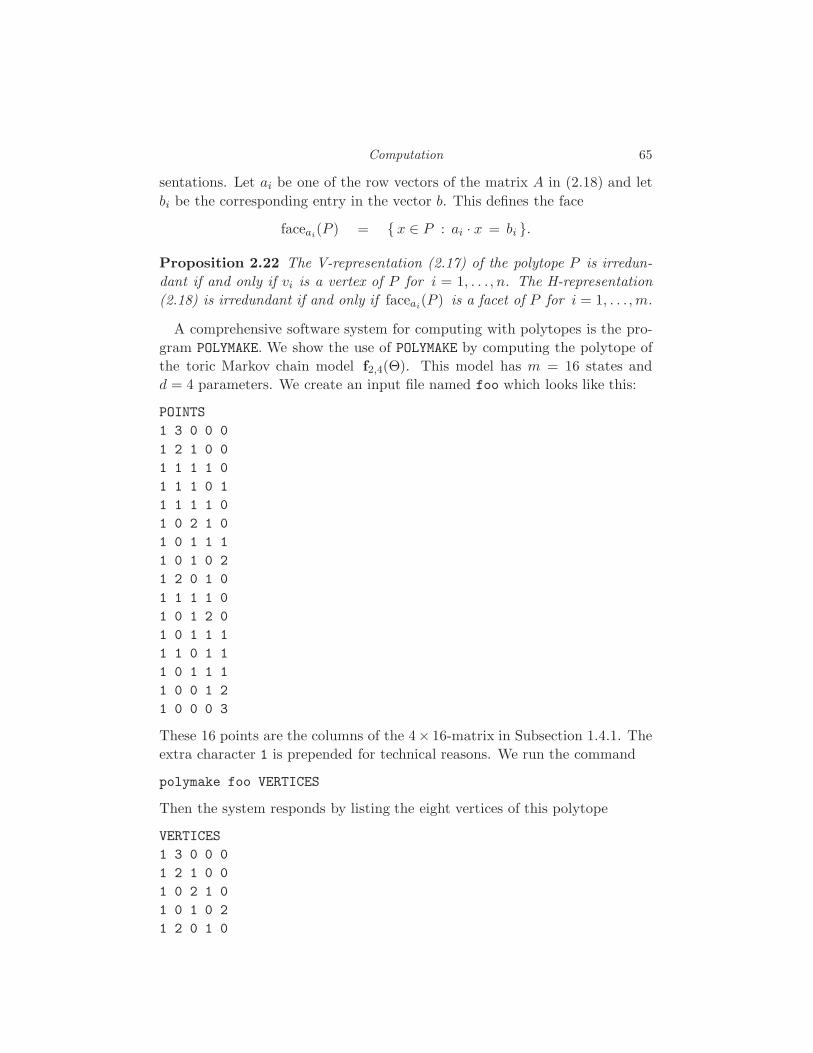
Computation 65
sentations. Let ai be one of the row vectors of the matrix A in (2.18) and let
bi be the corresponding entry in the vector b. This defines the face
faceai(P ) = x ∈ P : ai · x = bi .
Proposition 2.22 The V-representation (2.17) of the polytope P is irredun-
dant if and only if vi is a vertex of P for i = 1, . . . , n. The H-representation
(2.18) is irredundant if and only if faceai(P ) is a facet of P for i = 1, . . . , m.
A comprehensive software system for computing with polytopes is the pro-
gram POLYMAKE. We show the use of POLYMAKE by computing the polytope of
the toric Markov chain model f2,4(Θ). This model has m = 16 states and
d = 4 parameters. We create an input file named foo which looks like this:
POINTS
1 3 0 0 0
1 2 1 0 0
1 1 1 1 0
1 1 1 0 1
1 1 1 1 0
1 0 2 1 0
1 0 1 1 1
1 0 1 0 2
1 2 0 1 0
1 1 1 1 0
1 0 1 2 0
1 0 1 1 1
1 1 0 1 1
1 0 1 1 1
1 0 0 1 2
1 0 0 0 3
These 16 points are the columns of the 4× 16-matrix in Subsection 1.4.1. The
extra character 1 is prepended for technical reasons. We run the command
polymake foo VERTICES
Then the system responds by listing the eight vertices of this polytope
VERTICES
1 3 0 0 0
1 2 1 0 0
1 0 2 1 0
1 0 1 0 2
1 2 0 1 0

66 L. Pachter and B. Sturmfels
1 0 1 2 0
1 0 0 1 2
1 0 0 0 3
Furthermore, on the file foo itself we find the irredundant H-representation
FACETS
1 0 -1 1 0
0 1 0 0 0
1 0 1 -1 0
0 0 1 0 0
0 0 0 1 0
3 -1 -1 -1 0
AFFINE_HULL
-3 1 1 1 1
This output tells us that our polytope is defined by the one linear equation
x1 + x2 + x3 + x4 = 3 and the six linear inequalities
x2 − x3 ≤ 1, x1 ≥ 0, x3 − x2 ≤ 1, x2 ≥ 0, x3 ≥ 0, x1 + x2 + x3 ≤ 3.
Indeed, the command DIM confirms that the polytope is three-dimensional:
polymake foo DIM
DIM
3
The f-vector of our polytope coincides with that of the three-dimensional cube
polymake foo F_VECTOR
F_VECTOR
8 12 6
But our polytope is not a cube at all. Inspecting the updated file foo reveals
that its facets are two triangles, two quadrangles and two pentagons:
VERTICES_IN_FACETS
1 2 3
2 3 5 6 7
4 5 6
0 4 6 7
0 1 3 7
0 1 2 4 5
This is the polytope depicted in Figure 1.1. We return to our general discussion.
Computation 67
Let Pd denote the set of all polytopes in Rd. There are two natural oper-
ations, namely addition ⊕ and multiplication ⊙, defined on the set Pd. The
resulting structure is the polytope algebra(Pd,⊕,⊙
). Namely, if P,Q ∈ Pd are
polytopes then their sum P ⊕Q is the convex hull of the union of P and Q:
P ⊕Q := conv(P ∪ Q)
=λp+ (1− λ)q ∈ Rd : p ∈ P, q ∈ Q, 0 ≤ λ ≤ 1
.
The product in the polytope algebra is defined to be the Minkowski sum:
P ⊙Q := P + Q
=p+ q ∈ Rd : p ∈ P, q ∈ Q
.
It follows from the Weyl-Minkowski Theorem that both P ⊕Q and P ⊙Q are
polytopes in Rd. The polytope algebra(Pd,⊕,⊙
)satisfies many of the familiar
axioms of arithmetic. Clearly, addition and multiplication are commutative.
But it is also the case that the distributive law holds for polytopes:
Proposition 2.23 If P, Q, R are polytopes in Rd then
(P ⊕ Q) ⊙ R = (P ⊙ R) ⊕ (Q ⊙ R). (2.20)
Proof Consider points p ∈ P , q ∈ Q and r ∈ R. For 0 ≤ λ ≤ 1 note that
(λp + (1 − λ)q) + r = λ(p+ r) + (1− λ)(q + r).
The left hand side represents an arbitrary point in the left hand side of (2.20),
and the right hand side represents a point in the right hand side of (2.20).
Example 2.24 (The tropical semiring revisited) Let us consider the algebra
(P1,⊕,⊙) of all polytopes on the real line (d = 1). Each element of P1 is a
segment [a, b] where a < b are real numbers. The arithmetic operations are
[a, b] ⊕ [c, d] = [ min(a, c),max(b, d) ],
[a, b] ⊙ [c, d] = [ a+ c, b+ d ].
Thus the one-dimensional polytope algebra is essentially the same as the tropi-
cal semiring (R,⊕,⊙). Or, stated differently, the polytope algebra (Pd,⊕,⊙)
is a natural higher-dimensional generalization of the tropical semiring.
One of the main connections between polytopes and algebraic statistics is
via the Newton polytopes of the polynomials which parameterize a model.
Consider the polynomial
f =
n∑
i=1
ci · θvi11 θvi2
2 · · ·θvidd , (2.21)
68 L. Pachter and B. Sturmfels
where ci is a non-zero real number and vi = (vi1, vi2, . . . , vid) ∈ Nd for i =
1, 2, . . . , n. We define the Newton polytope of the polynomial f as the convex
hull of all exponent vectors that appear in the expansion (2.21) of f :
NP(f) := convv1, v2, . . . , vn ⊂ Rd. (2.22)
Hence the Newton polytope NP(f) is precisely the V-polytope in (2.17). The
operation of taking Newton polytopes respects the arithmetic operations:
Theorem 2.25 Let f and g be polynomials in R[θ1, . . . , θd]. Then
NP(f · g) = NP(f) ⊙ NP(g) and NP(f + g) ⊆ NP(f) ⊕ NP(g).
If all coefficients of f and g are positive then NP(f + g) = NP(f) ⊕ NP(g).
Proof Let f =∑n
i=1 ci · θvi be as in (2.21) and let g =∑n′
j=1 c′j · θv′j . For any
w ∈ Rd let inw(f) denote the initial form of f . This is the subsum of all terms
ciθvi such that vi · w is minimal. Then the following identity holds:
NP(inw(f)
)= facew
(NP(f)
). (2.23)
The initial form of a product is the product of the initial forms:
inw(f · g) = inw(f) · inw(g). (2.24)
For generic w ∈ Rd, the initial form (2.24) is a monomial θvi+v′j , and its
coefficient in f · g is the product of the corresponding coefficients in f and g.
Finally, the face operator facew( · ) is a linear map on the polytope algebra:
facew
(NP(f) ⊙ NP(g)
)= facew
(NP(f)
)⊙ facew
(NP(g)
). (2.25)
Combining the three identities (2.23), (2.24) and (2.25), for w generic, shows
that the polytopes NP(f ·g) and NP(f)⊙ NP(g) have the same set of vertices.
For the second identity, note that NP(f) ⊕ NP(g) is the convex hull of
v1, . . . , vn, v′1, . . . , v
′n′. Every term of f + g has its exponent in this set, so
this convex hull contains NP(f+g). If all coefficients are positive then equality
holds because there is no cancellation when forming the sum f + g.
Example 2.26 Consider the polynomials f = (x+1)(y+1)(z+1) and g = (x+
y + z)2. Then NP(f) is a cube and NP(g) is a triangle. The Newton polytope
NP(f+g) of their sum is the bipyramid with vertices (0, 0, 0), (2, 0, 0), (0, 2, 0),
(0, 0, 2), (1, 1, 1). The Newton polytope NP(f · g) of their product is the
Minkowski sum of the cube with the triangle. It has 15 vertices.
Computation 69
Newton polytopes allow us to transfer constructions from the algebraic set-
ting of polynomials to the geometric setting of polytopes. To illustrate consider
the following example. Suppose we are given a 4 × 4 matrix of polynomials,
A(x, y, z) =
a11(x, y, z) a12(x, y, z) a13(x, y, z) a14(x, y, z)
a21(x, y, z) a22(x, y, z) a23(x, y, z) a24(x, y, z)
a31(x, y, z) a32(x, y, z) a33(x, y, z) a34(x, y, z)
a41(x, y, z) a42(x, y, z) a43(x, y, z) a44(x, y, z)
,
and suppose we are interested in the Newton polytope of its determinant
det(A(x, y, z)
). One possible way to compute this Newton polytope is to
evaluate the determinant, list all terms that occur in that polynomial, and
then compute the convex hull. However, assuming that the coefficients of the
aij(x, y, z) are such that no cancellations occur, it is more efficient to do the
arithmetic directly at the level of Newton polytopes. Namely, we replace each
matrix entry by its Newton polytope Pij = NP(aij), consider the 4×4 matrix
of polytopes (Pij), and compute its determinant in the polytope algebra. Just
like in the tropical semiring (2.6), here the determinant equals the permanent:
det
P11 P12 P13 P14
P21 P22 P23 P24
P31 P32 P33 P34
P41 P42 P43 P44
=
⊕
σ∈S4
P1σ(1) ⊙ P2σ(2) ⊙ P3σ(3) ⊙ P4σ(4).
This determinant of polytopes represents a parameterized family of assignment
problems. Indeed, suppose the cost qij of assigning job i to worker j depends
piecewise-linearly on a vector of three parameters w = (wx, wy, wz), namely
qij = minw · p : p ∈ Pij.
Thus the cost qij is determined by solving the linear programming problem
with polytope Pij . The parametric assignment problem would be to solve the
assignment problem simultaneously for all vectors w ∈ R3. In other words, we
wish to preprocess the problem specification so that the cost of an optimal as-
signment can be computed rapidly. This preprocessing amounts to computing
the irredundant V-representation of the polytope gotten from the determinant.
Then the cost of an optimal assignment can be computed as follows:
minw · p : p ∈ det((Pij)1≤i,j≤4
).
Our discussion furnishes a higher-dimensional generalization of Remark 2.6:
Remark 2.27 The parametric assignment problem is solved by computing
the determinant of the matrix of polytopes (Pij) in the polytope algebra.

70 L. Pachter and B. Sturmfels
We can similarly define the parametric shortest path problem on a directed
graph. The weight of each edge is now a polytope Pij in Rd, and for a specific
parameter vector w ∈ Rd we recover the scalar edge weights by linear pro-
gramming on that polytope: dij = minw · p : p ∈ Pij. Then the shortest
path from i to j is given by d(n−1)ij = minw · p : p ∈ P
(n−1)ij , where P
(n−1)ij
is the (i, j)-entry in the (n − 1)-st power of the matrix (Pij). Here matrix
multiplication is carried out in the polytope algebra(Pd,⊕,⊙
).
The Hungarian algorithm for assignments and the Floyd-Warshall algorithm
for shortest paths can be extended to the parametric setting. Provided the
number d of parameters is fixed, these algorithms still run in polynomial time.
The efficient computation of such polytopes by dynamical programming using
polytope algebra arithmetic along a graph is referred to as polytope propagation
(see Chapters 5–8). We close this section by revisiting the case of alignments.
Remark 2.28 The problem of parametric alignment of two DNA sequences
σ1 and σ2 is to compute the Newton polytopes NP(fσ1,σ2) of the corresponding
coordinate polynomial fσ1,σ2 of the pair hidden Markov model (2.13).
If some of the scores have been specialized then we compute Newton poly-
topes of polynomials in fewer unknowns. For instance, if w′ = 0 then our
task is to compute the Newton polytope NP(gσ1,σ2) of the specialized poly-
nomial gσ1,σ2 . This can be done efficiently by running the Needleman-Wunsch
Algorithm 2.13 in the polytope algebra and is the topic of Chapters 5–7.
Example 2.29 Returning to Example 2.18, we observe that the 14 points
v1, . . . , v14 are the vertices of the Newton polytope P = NP(gACG,ACC). It is
important to note that all of the 14 points corresponding to monomials in
gACG,ACC are in fact vertices of P , which means that every possible alignment of
ACG and ACC is an optimal alignment for some choice of parameters.
The polytope P is easily computed in POLYMAKE, which confirms that the
polytope is six-dimensional. The f-vector is f(P ) = (14, 51, 86, 78, 39, 10).
These numbers have an interpretation in terms of alignments. For example,
there is an edge between two vertices in the polytope if for two different optimal
alignments (containing different numbers of matches, mismatches, and gaps)
the parameter regions which yield the optimal alignments share a boundary.
In other words, the fact that the polytope has 51 edges tells us that there
are precisely 51 “parameter boundaries”, where an infinitesimal change in pa-
rameters can result in a different optimal alignment. The normal cones and
their defining inequalities (like the seven in Example 2.18) characterize these
boundaries, thus offering a solution to the parametric alignment problem.

Computation 71
2.4 Trees and metrics
One of the important mathematical structures that arises in biology is the
phylogenetic tree [Darwin, 1859, Felsenstein, 2003, Semple and Steel, 2003]. A
phylogenetic tree is a tree T together with a labeling of its leaves. The number
of combinatorial types of phylogenetic trees with the same leaves grows expo-
nentially (Lemma 2.32). In phylogenetics a typical problem is to select a tree,
based on data, from the large number of possible choices.
This section introduces some basic concepts in combinatorics of trees that
are important for phylogeny. The notion of tree space is related to the tropi-
calization principle introduced in Section 2.1 and will be revisited in Section
3.5. A widely used algorithm in phylogenetics, the neighbor joining algorithm,
is a method for projecting a metric onto tree space. This algorithm draws on a
number of ideas in phylogenetics and serves as the focus of our presentation in
this section. We begin by discussing a number of different, yet combinatorially
equivalent, characterizations of trees.
A dissimilarity map on [n] = 1, 2, . . . , n is a function d : [n] × [n] → Rsuch that d(i, i) = 0 and d(i, j) = d(j, i) ≥ 0. The set of all dissimilarity maps
on [n] is a real vector space of dimension(n2
), which we identify with R(n
2). A
dissimilarity map d is called a metric on [n] if the triangle inequality holds:
d(i, j) ≤ d(i, k) + d(k, j) for i, j, k ∈ [n]. (2.26)
A dissimilarity map d can be written as a non-negative symmetric n×n matrix
D = (dij) where dij = d(i, j) and dii = 0. The triangle inequality (2.26) can
be expressed by matrix multiplication where the arithmetic is tropical.
Remark 2.30 The matrix D represents a metric if and only if D ⊙D = D.
Proof The entry of the matrix D ⊙D in row i and column j equals
di1 ⊙ d1j ⊕ · · · ⊕ din ⊙ dnj = mindik + dkj : 1 ≤ k ≤ n
. (2.27)
This quantity is less than or equal to dij = dii ⊙dij = dij ⊙djj, and it equals
dij if and only if the triangle inequality dij ≤ dik + dkj holds for all k.
The set of all metrics on [n] is a full-dimensional convex polyhedral cone
in R(n2), called the metric cone. The metric cone has a distinguished subcone,
known as the cut cone, which is the R≥0-linear span of all metrics dA,B arising
as follows from all splits A,B of [n] into two non-empty subsets A and B:
dA,B(i, j) = 1 if i, j ∈ A or i, j ∈ B
dA,B(i, j) = 0 if i ∈ A, j ∈ B or i ∈ B, j ∈ A.(2.28)
The cut cone is strictly contained in the metric cone if n ≥ 6. This and many
other results on metrics can be found in [Deza and Laurent, 1997].
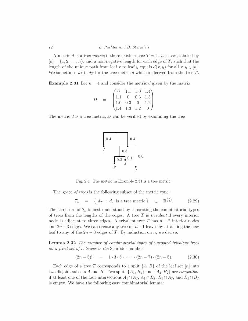
72 L. Pachter and B. Sturmfels
A metric d is a tree metric if there exists a tree T with n leaves, labeled by
[n] = 1, 2, . . . , n, and a non-negative length for each edge of T , such that the
length of the unique path from leaf x to leaf y equals d(x, y) for all x, y ∈ [n].
We sometimes write dT for the tree metric d which is derived from the tree T .
Example 2.31 Let n = 4 and consider the metric d given by the matrix
D =
0 1.1 1.0 1.4
1.1 0 0.3 1.3
1.0 0.3 0 1.2
1.4 1.3 1.2 0
The metric d is a tree metric, as can be verified by examining the tree
b
b
4
0.4
b
0.4
b
0.3
b
2
0.2 b
3
0.1
b
1
0.6
Fig. 2.4. The metric in Example 2.31 is a tree metric.
The space of trees is the following subset of the metric cone:
Tn =dT : dT is a tree metric
⊂ R(n
2). (2.29)
The structure of Tn is best understood by separating the combinatorial types
of trees from the lengths of the edges. A tree T is trivalent if every interior
node is adjacent to three edges. A trivalent tree T has n − 2 interior nodes
and 2n−3 edges. We can create any tree on n+1 leaves by attaching the new
leaf to any of the 2n− 3 edges of T . By induction on n, we derive:
Lemma 2.32 The number of combinatorial types of unrooted trivalent trees
on a fixed set of n leaves is the Schroder number
(2n− 5)!! = 1 · 3 · 5 · · · · · (2n− 7) · (2n− 5). (2.30)
Each edge of a tree T corresponds to a split A,B of the leaf set [n] into
two disjoint subsets A and B. Two splits A1, B1 and A2, B2 are compatible
if at least one of the four intersections A1 ∩A2, A1 ∩B2, B1 ∩A2, and B1 ∩B2
is empty. We have the following easy combinatorial lemma:

Computation 73
Lemma 2.33 If A1, B1 and A2, B2 are splits corresponding to two edges
on a tree T with leaf set [n] then A1, B1 and A2, B2 are compatible.
Let A1, B1 and A2, B2 be two distinct compatible splits. We say that
A1 is mixed with respect to A2, B2 if A1∩A2 and A1∩B2 are both nonempty.
Otherwise A1 is pure with respect to A2, B2. Of the two components A1 and
B1 exactly one is pure and the other is mixed with respect to the other split
A2, B2. Let Splits(T ) denote the collection of all 2n−3 splits (A,B) arising
from T . For instance, if n = 4 and T is the tree in Figure 2.4 then
Splits(T ) =1, 234, 14, 23, 123, 4, 134, 2, 124, 3
. (2.31)
Theorem 2.34 (Splits Equivalence Theorem) A collection S of splits is
pairwise compatible if and only if there exists a tree T such that S = Splits(T ).
Moreover, if such a tree T exists then it is unique.
Proof If there are no splits then the tree is a single node. Otherwise, we proceed
by induction. Consider the set of splits S ′ = S\A,B where A,B is a
split in S. There is a unique tree T ′ corresponding to the set of splits S ′. Any
split in S ′ has one pure and one mixed component with respect to A,B.We orient the corresponding edge e of T ′ so that it is directed from the pure
component to the mixed component. We claim that no node in T ′ can have
out-degree ≥ 2. If this was the case there would be a split with a component
that is both pure and mixed with respect to (A,B). Thus every node of T ′
has out-degree either 0 or 1. Since the number of nodes is one more than the
number of edges, we conclude that the directed tree T ′ has a unique sink v′.
Replace v′ with two new nodes vA and vB and add a new edge between them
as indicated in Figure 2.5. The result is the unique tree T with S = Splits(T ).
We next establish the classical four point condition which characterizes mem-
bership in tree space Tn. The proof is based on the notion of a quartet, which
for any phylogenetic tree T is a subtree spanned by four taxa i, j, k, l. Ifi, j, k, l
is a split of that subtree then we denote the quartet by (ij; kl).
Theorem 2.35 (The four point condition) A metric d is a tree metric if
and only if, for any four leaves u, v, x, y, the maximum of the three numbers
d(u, v)+d(x, y), d(u, x)+d(v, y) and d(u, y)+d(v, x) is attained at least twice.
Proof If d = dT for some tree then for any quartet (uv; xy) of T it is clear that
d(u, v) + d(x, y) ≤ d(u, x) + d(v, y) = d(u, y) + d(v, x).
Hence the “only if” direction holds.
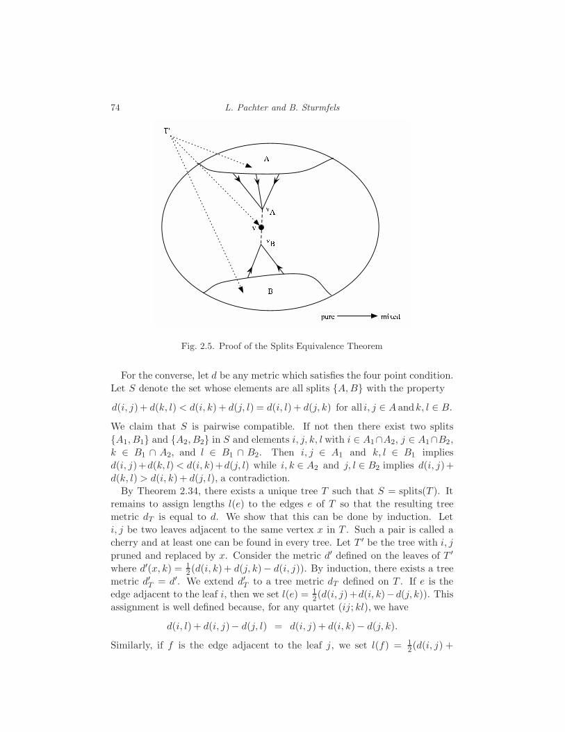
74 L. Pachter and B. Sturmfels
p u r e m i x e d
A
Bv Av Bv
T '
Fig. 2.5. Proof of the Splits Equivalence Theorem
For the converse, let d be any metric which satisfies the four point condition.
Let S denote the set whose elements are all splits A,B with the property
d(i, j)+ d(k, l) < d(i, k) + d(j, l) = d(i, l) + d(j, k) for all i, j ∈ A andk, l ∈ B.
We claim that S is pairwise compatible. If not then there exist two splits
A1, B1 and A2, B2 in S and elements i, j, k, l with i ∈ A1∩A2, j ∈ A1∩B2,
k ∈ B1 ∩ A2, and l ∈ B1 ∩ B2. Then i, j ∈ A1 and k, l ∈ B1 implies
d(i, j)+d(k, l)< d(i, k)+d(j, l) while i, k ∈ A2 and j, l ∈ B2 implies d(i, j)+
d(k, l) > d(i, k) + d(j, l), a contradiction.
By Theorem 2.34, there exists a unique tree T such that S = splits(T ). It
remains to assign lengths l(e) to the edges e of T so that the resulting tree
metric dT is equal to d. We show that this can be done by induction. Let
i, j be two leaves adjacent to the same vertex x in T . Such a pair is called a
cherry and at least one can be found in every tree. Let T ′ be the tree with i, j
pruned and replaced by x. Consider the metric d′ defined on the leaves of T ′
where d′(x, k) = 12 (d(i, k)+ d(j, k)− d(i, j)). By induction, there exists a tree
metric d′T = d′. We extend d′T to a tree metric dT defined on T . If e is the
edge adjacent to the leaf i, then we set l(e) = 12(d(i, j)+d(i, k)−d(j, k)). This
assignment is well defined because, for any quartet (ij; kl), we have
d(i, l) + d(i, j)− d(j, l) = d(i, j) + d(i, k)− d(j, k).
Similarly, if f is the edge adjacent to the leaf j, we set l(f) = 12(d(i, j) +
Computation 75
d(j, k) − d(i, k)). Since dT (i, j) = l(e) + l(f) it follows that dT (i, j) = d(i, j).
Similarly, for any k 6= i, j, dT (i, k) = d(i, k) and dT (j, k) = d(j, k).
The previous argument shows that the set of split metricsdA,B : (A,B) ∈ Splits(T )
(2.32)
is linearly independent in R(n2). We wrote the tree metric dT uniquely as a
linear combination of this set of split metrics. Let CT denote the non-negative
span of the set (2.32). The cone CT is isomorphic to the orthant R2n−3≥0 .
Proposition 2.36 The space of trees Tn is the union of the (2n−5)!! orthants
CT . More precisely, Tn is a simplicial fan of pure dimension 2n− 3 in R(n2).
We return to tree space (and its relatives) in Section 3.5, where we show
that Tn can be interpreted as a Grassmannian in tropical algebraic geometry.
The relevance of tree space to efficient statistical computation is this: sup-
pose that our data consists of measuring the frequency of occurrence of the
different words in A, C, G, Cn as columns of an alignment on n DNA se-
quences. As discussed in Section 1.4, we would like to select a tree model. In
principle, we could compute the MLE for each of the (2n − 5)!! trees, how-
ever, this approach has a number of difficulties. First, even for a single tree
the MLE computation is very difficult, even if we are satisfied with a reason-
able local maximum of the likelihood function. Even if the MLE computa-
tion were feasible, a naive approach to model selection requires examining all
exponentially many (in n) trees. One popular way to avoid these problems
is the “distance based approach” which is to collapse the data to a dissim-
ilarity map and then to obtain a tree via a projection onto tree space (see
4.21). The projection of choice for most biologists is the neighbor joining al-
gorithm which provides an easy-to-compute map from the metric cone onto
Tn. The algorithm is based on Theorem 2.35 and the Cherry Picking Theorem
[Saitou and Nei, 1987, Studier and Keppler, 1988].
Fix a dissimilarity map d on the set [n]. For any a1, a2, b1, b2 ∈ [n] we set
w(a1a2; b1b2) :=14 [d(a1, b1) + d(a1, b2) + d(a2, b1) + d(a2, b2) − 2[d(a1, a2) + d(b1, b2)]].
The function w provides a natural “weight” for quartets when d is a tree metric.
The following result on quartets is proved by inspecting a tree with four leaves.
Lemma 2.37 If d is a tree metric with (a1a2; b1b2) a quartet in the tree, then
w(a1a2; b1b2) = −2 · w(a1b1; a2b2), and this number is the length of the path
which connects the path between a1 and a2 with the path between b1 and b2.

76 L. Pachter and B. Sturmfels
A cherry of a tree is a pair of leaves which are both adjacent to the same
node. The following theorem gives a criterion for identifying cherries.
Theorem 2.38 (Cherry picking theorem) If d is a tree metric on [n] and
Zd(i, j) =∑
k,l∈[n]\i,j
w(ij; kl) (2.33)
then any pair of leaves that maximizes Zd(i, j) is a cherry in the tree.
Proof Suppose that i, j is not a cherry in the tree. Without loss of generality,
we may assume that either there is a leaf k forming a cherry with i, or neither
i nor j form a cherry with any leaf. In the first case, observe that
Zd(i, k)− Zd(i, j) =∑
x,y 6=i,j,k
(w(ik; xy)−w(ij; xy))
+∑
x 6=i,j,k
(w(ik; xj)−w(ij; xk)) > 0.
Here we are using Lemma 2.37. In the latter case, there must be cherries (k, l)
and (p, q) arranged as in Figure 2.6. Without loss of generality, we assume
that the cherry (k, l) has the property that the number of leaves in T \ e in the
same component as k is less than or equal to the number of leaves in T \ e′ inthe same component as p. We now compare Zd(k, l) to Zd(i, j):
Zd(k, l)− Zd(i, j) =∑
x,y 6=i,j,k,l
(w(kl; xy)− w(ij; xy))
+∑
x 6=i,j,k,l
(w(kl; xj)+ w(kl; ix)− w(ij; xl)−w(ij; kx)).
The two sums are each greater than 0. In the first sum, we need to evaluate
all possible positions for x and y within the tree. If, for example, x and y
lie in the component of T\x, y that contains i and j then it is clear that
w(kl; xy)−w(ij; xy)> 0. If x and y lie in the same component of T \ e as leaf
k, then it may be that w(kl; xy) − w(ij; xy) < 0, however for each such pair
x, y there will be another pair that lies in the same component of T \ e′ as leaf
p. The deficit for the former pair will be less than the surplus provided by the
second. The remaining cases follow directly from Lemma 2.37.
Theorem 2.38 is conceptually simple and useful, and we will see that it is
useful for understanding the neighbor joining algorithm. It is however not
computationally efficient because O(n2) additions are necessary just to find
one cherry. An equivalent, but computationally superior, formulation is:

Computation 77i jk i jk l
ep q
e 'Fig. 2.6. Cases in the proof of the Cherry Picking Theorem.
Corollary 2.39 Let d be a tree metric on [n]. For every pair i, j ∈ [n] set
Qd(i, j) = (n− 2) · d(i, j) −∑
k 6=i
d(i, k) −∑
k 6=j
d(j, k). (2.34)
Then the pair x, y ∈ [n] that minimizes Qd(x, y) is a cherry in the tree.
Proof Let τ =∑
x,y∈[n] d(x, y). A direct calculation reveals the identity
Zd(i, j) = − 1
2· τ − n− 2
2·Qd(i, j).
Thus maximizing Zd(x, y) is equivalent to minimizing Qd(x, y).
The neighbor joining algorithm makes use of the cherry picking theorem by
peeling off cherries to recursively build a tree:
Algorithm 2.40 (Neighbor joining algorithm)
Input: A dissimilarity map d on the set [n].
Output: A phylogenetic tree T whose tree metric dT is “close” to d.
Step 1: Construct the n × n matrix Qd whose (i, j)-entry is given by the
formula (2.34), and identify the minimum off-diagonal entry Qd(x, y).
Step 2: Remove x, y from the tree and replace them with a new leaf z. For
78 L. Pachter and B. Sturmfels
each leaf k among the the remaining n− 2 leaves, set
d(z, k) =1
2
(d(x, k) + d(y, k)− d(x, y)
). (2.35)
This replaces the n× n matrix Qd by an (n− 1)× (n− 1) matrix. Return to
Step 1 until there are no more leaves to collapse.
Step 3: Output the tree T . The edge lengths of T are determined recursively: If
(x, y) is a cherry connected to node z as in Step 2, then the edge from x to z has
length d(x, k)−dT (z, k) and the edge from y to z has length d(y, k)−dT (z, k).
This neighbor joining algorithm recursively constructs a tree T whose metric
dT is hopefully close to the given metric d. If d is a tree metric to begin with
then the method is guaranteed to reconstruct the correct tree. More generally,
instead of estimating pairwise distances, one can attempt to (more accurately)
estimate the sum of the branch lengths of subtrees of size m ≥ 3.
For any positive integer d ≥ 2, we define a d-dissimilarity map on [n] to be
a function D : [n]d → R such that D(i1, i2, . . . , id) = D(iπ(1), iπ(2), . . . , iπ(d))
for all permutations π on 1, . . . , d and D(i1, i2, . . . , id) = 0 if the taxa
i1, i2, . . . , id are not distinct. The set of all d-dissimilarity maps on [n] is a real
vector space of dimension(nd
)which we identify with R(n
d). Every tree T gives
rise to an d-dissimilarity map DT as follows. We define DT (i1, . . . , id) to be
the sum of all branch lengths in the subtree of T spanned by i1, . . . , id ∈ [n].
The following theorem is a generalization of Corollary 2.39. It leads to a
generalized neighbor joining algorithm which provides a better approximation
of the maximum likelihood tree and parameters. A proof is given in Chapter
18 together with an explanation of the relevance of algebraic techniques for
maximum likelihood estimation.
Theorem 2.41 Let T be a tree on [n] and d < n. For any i, j ∈ [n] set
QT (i, j) =
(n− 2
d− 1
) ∑
Y ∈([n]\i,jd−2 )
DT (i, j, Y ) −∑
Y ∈([n]\id−1 )
DT (i, Y ) −∑
Y ∈([n]\jd−1 )
DT (j, Y ).
Then the pair x, y ∈ [n] that minimizes QT (x, y) is a cherry in the tree T .
The subset of R(nd) consisting of all d-dissimilarity maps DT arising from
trees T is a polyhedral space which is the image of the tree space Tn under a
linear map R(n2) → R(n
d). This polyhedral space is related to the tropicalization
of the Grassmannian Gd,n, which is discussed in Section 3.5, but the details of
this relationship are still not fully understood and deserve further study.

Computation 79
2.5 Software
In this section we introduce the software packages which were used by the
authors of this book. These programs were discussed in our seminar in the
Fall of 2004 and they played a key role for the studies which are presented
in part 2 of this book. The subsection on Mathematical Software describes
packages traditionally used by mathematicians but which may actually be very
useful for statisticians and biologists. The section on Computational Biology
Software summarizes programs more traditionally used for biological sequence
analysis. In each subsection the software packages are listed in alphabetic order
by name. Short examples or pointers to such examples are included for each
package. These illustrate how the software was used in our computations.
2.5.1 Mathematical Software
We describe ten packages for mathematical calculations relevant for this book.
4TI2
Summary: A package for linear algebra over the non-negative integers (e.g. in-
teger programming). Very useful for studying toric models (Section 2.2).
Example: To solve the linear equation 2x + 5y = 3u + 4v for non-negative
integers x, y, u, v we create a file named foo with the following two lines
1 4 2 5 -3 -4
Running the command hilbert foo creates a 10×4 matrix on a file foo.hil:
10 4
2 0 0 1
3 0 2 0
1 1 1 1
2 1 3 0
1 2 0 3
0 2 2 1
1 2 4 0
0 3 1 3
0 3 5 0
0 4 0 5
Every solution to the equation is an N-linear combination of these ten rows.
Availability: Executable only.
Website: www.4ti2.de/

80 L. Pachter and B. Sturmfels
LINPACK
Summary: A Fortran library for linear algebra, originally from the 1970s but
still widely used for scientific computation. It contains fast implementations
of certain linear algebra algorithms, such as singular value decomposition.
Example: The singular value decomposition subroutine in LINPACK is used in
Chapter 19 to construct phylogenetic trees from alignments of DNA sequences.
Availability: Open source.
Website: www.netlib.org/linpack/
MACAULAY2
Summary: A software system supporting research in algebraic geometry and
commutative algebra [Grayson and Stillman, 2002].
Example: We illustrate the computation of toric models in MACAULAY2. Con-
sider the toric Markov chain of length n = 4 with alphabet Σ = 0, 1 that
appears in Subsection 1.4.2. The model is specified with the commands:
i1 : R = QQ[p0000,p0001,p0010,p0011, p0100,p0101,p0110,p0111,
p1000,p1001,p1010,p1011, p1100,p1101,p1110,p1111];
i2 : S = QQ[a00,a01,a10,a11];
i3 : f = map(S,R, a00*a00*a00, a00*a00*a01, a00*a01*a10,
a00*a01*a11, a01*a10*a00, a01*a10*a01, a01*a11*a10,
a01*a11*a11, a10*a00*a00, a10*a00*a01, a10*a01*a10,
a10*a01*a11, a11*a10*a00, a11*a10*a01, a11*a11*a10,
a11*a11*a11);
o3 : RingMap S <--- R
We have used the indeterminates a00,a01,a10,a11 for the parameters
θ =
(θ00 θ01
θ10 θ11
).
The labels i1,i2,i3 indicate input to the program, o3 is output generated by
MACAULAY2. We compute a Grobner basis for the ideal If (see Section 3.2):
i4 : time If = kernel(f); -- Used 0.88 seconds
o4 : Ideal of R
i5 : gb If
o5 = | p1011-p1101 p0110-p1101 p0100-p1001 p0010-p1001
Computation 81
p1101p1110-p1010p1111 p0111p1110-p1101p1111
p0011p1110-p1001p1111 p1101^2-p0101p1110
p1100p1101-p1001p1110 p0111p1101-p0101p1111
p1100^2-p1000p1110 p1001p1100-p1000p1101
p0111p1100-p1001p1111 p0101p1100-p1001p1101
p0011p1100-p0001p1110 p0001p1100-p0000p1101
p0111p1010-p0101p1110 p0011p1010-p1001p1101
p1001^2-p0001p1010 p1000p1001-p0000p1010
p0111p1001-p0011p1101 p0011p1001-p0001p1101
p0111p1000-p0001p1110 p0101p1000-p0001p1010
p0011p1000-p0000p1101 p0001p1000-p0000p1001
p0000p0101-p0001p1001 p0011^2-p0001p0111
p0101p1110^2-p1010p1101p1111 p1001p1110^2-p1010p1100p1111
p0001p1110^2-p1000p1101p1111 p0000p1010p1100-p1000^2p1101
p0000p0011p1101-p0001^2p1110 p0000p1110^2-p1000p1100p1111
p0000p1100p1110-p1000^2p1111 p0000p0111^2-p0001p0011p1111
p0000p0011p0111-p0001^2p1111 |
These are the constraints on probabilities listed at the end of Subsection 1.4.1.
Availability: Open source.
Website: www.math.uiuc.edu/Macaulay2/
MAGMA
Summary: A software package for computation with algebraic, geometric and
combinatorial structures such as graphs, groups, rings and fields. Includes a
new fast implementation of the Faugere F4 algorithm for computing Grobner
bases [Bosma et al., 1997].
Example: We compute a Grobner basis for the example in Section 3.1.
Q := RationalField();
P<p1,p2,p3> := PolynomialRing(Q, 3);
I := ideal<P | p1^4+p2^4-p3^4,p1^4+p2^4+p3^4-2*p1*p2*p3,p1+p2+p3-1>;
G := GroebnerBasis(I);
G;
[ p1 + p2 + p3 - 1,
p2^4 - 2*p2^3 + 3*p2^2 - 2*p2*p3^4 + p2*p3^3 - p2*p3^2 + 2*p2*p3
- 2*p2 - p3^5 + 4*p3^4 - 2*p3^3 + 3*p3^2 - 2*p3 + 1/2,
p2^2*p3 + p2*p3^2 - p2*p3 + p3^4,
p3^7 - 2*p3^6 + 4*p3^5 - 4*p3^4 + 3*p3^3 - 2*p3^2 + 1/2*p3 ]
Availability: Commercial software.
Website: magma.maths.usyd.edu.au/magma/

82 L. Pachter and B. Sturmfels
MAPLE
Summary:General purpose platform for symbolic and numerical computation
Example: MAPLE is an extremely versatile and powerful system, which includes
many toolboxes and routines for standard symbolic and numerical computa-
tions. It is also an intuitive high-level interpreted language, which is convenient
for quick computations. In Section 2.2, a specific example is provided showing
how to compute sequence alignment polynomials using MAPLE.
Availability: Commercial software.
Website: www.maplesoft.com/
MATHEMATICA
Summary:General purpose platform for symbolic and numerical computation
Example: In Chapter 12 MATHEMATICA is used to plot the likelihood surface
for various hidden Markov models.
Availability: Commercial software.
Website: www.wolfram.com/products/mathematica/index.html
MATLAB
Summary: A general purpose high level mathematics package, particularly
suited towards numerical linear algebra computations. MATLAB is supported
by numerous specialized toolboxes: the statistics toolbox and bioinformatics
toolbox are useful for computational biology.
Example: The following example illustrates the use of the statistics toolbox
for experimenting with hidden Markov models. The example shows how to set
up a simple model with l = 2 and l′ = 4, generate data from the model, and
how to run basic inference routines.
S=[0.8 0.2; 0.1 0.9]
S = 0.8 0.2
0.1 0.9
T=[0.25 0.25 0.25 0.25; 0.125 0.375 0.375 0.125]
T =
0.250 0.250 0.250 0.250
0.125 0.375 0.375 0.125
These commands set up the matrices θ and θ′. In other words, we have fixed
a point on the model. The command hmmgenerate generates data from the
model, and also specifies the alphabets Σ and Σ′ to be used:

Computation 83
DNAseq=hmmgenerate(100,S,T,’Statenames’,’exon’,’intron’,
’Symbols’,’A’,’C’,’G’,’T’)
DNAseq =
Columns 1 through 14
’G’ ’C’ ’C’ ’C’ ’G’ ’A’ ’C’ ’G’ ’T’ ’C’ ’T’ ’A’ ’C’ ’C’
...
The probability of DNAseq given the model, i.e. the evaluation of the DNAseq
coordinate polynomial, is done with
[PSTATES,logpseq]=hmmdecode[DNAseq,S,T,’Symbols’,
’A’,’C’,’G’,’T’]
The matrix PSTATES returns the forward variables (see Chapter 12) . The
logarithm of the probability of the sequence is also returned:
logpseq =
-1.341061974974420e+02
The tropicalization of the coordinate polynomial is evaluated as follows:
STATES=hmmviterbi(DNAseq,S,T,’Statenames’,’exon’,’intron’,
’Symbols’,’A’,’C’,’G’,’T’
STATES =
Columns 1 through 7
’intron’ ’intron’ ’intron’ ’intron’ ’intron’ ’intron’ ’intron’
...
Columns 99 through 100
’exon’ ’exon’
The MATLAB statistics toolbox also has an implementation of the EM algorithm
for hidden Markov models, using the command hmmtrain.
Availability: Commercial software.
Website: www.mathworks.com/

84 L. Pachter and B. Sturmfels
POLYMAKE
Summary: A collection of programs for building, manipulating, analyzing
and otherwise computing with polytopes and related polyhedral objects
[Gawrilow and Joswig, 2000, Gawrilow and Joswig, 2001].
Example: Several computations with polytopes are shown in Section 2.3.
Availability: Open source.
Website: www.math.tu-berlin.de/polymake/
SINGULAR
Summary: A system for polynomial computations, commutative algebra, and
computational algebraic geometry. Very useful for algebraic statistics.
Example: See Sections 2.1, 2.2 and 2.3 for various examples. For a reference
on SINGULAR with many worked out examples see [Greuel and Pfister, 2002].
Availability: Free under the GNU (GNU’s Not Unix) Public License.
Website: www.singular.uni-kl.de/
R
Summary: A statistical computing language and environment, similar in
syntax and focus to the S language [Ihaka and Gentleman, 1996]. Mathe-
maticians find R comparable to MATLAB. The BIOCONDUCTOR package for R
[Gentleman et al., 2004] provides support for bioinformatics. related problems.
Example: The following R code was used to produce Figure 3.1:
# Hardy-Weinberg curve
p <- c(seq(0, 1, 0.001), seq(1, 100, 0.01))
z0 <- p^2/(1+p)^2
z1 <- 2*p/(1+p)^2
z2 <- 1/(1+p)^2
x.rec <- cbind((2*z0+z1)/sqrt(3), z1)
## plot the Hardy-Weinberg curve
plot(x.rec[,1], x.rec[,2], type=’l’, xlim=c(0, 2/sqrt(3)), ylim=c(0, 1), xlab=’’, ylab=’’,
# plot simplex
lines(x=c(0, 2/sqrt(3)), y=c(0, 0))
lines(x=c(0, 1/sqrt(3)), y=c(0, 1))
lines(x=c(1/sqrt(3), 2/sqrt(3)), y=c(1, 0))
Availability: Open source.
Website: www.r-project.org/
Computation 85
2.5.2 Computational Biology Software
The five software programs highlighted here were all used during the prepara-
tion of the book, and are mostly accessible through web servers.
BLAST
Summary: A tool for searching through large biological sequence databases
for matches to a query [Altschul et al., 1990].
Example: There are many different “flavors” of BLAST, which allow for query-
ing databases of DNA or protein, automatic translation of the input sequence,
and other similar modifications. In what follows we illustrate the use of the
BLASTN tool. We begin by submitting the sequence
ATGGCGGAGTCTGTGGAGCGCCTGCAGCAGCGGGTCCAGGAGCTGGAGCGGGAACTT
taken from an example in Section 7.4, to the BLASTN website. There are a
number of important variables that can be set for the search, for example: the
low complexity filter removes repeated subsequences, such as TTTT...TTT from
the search. The word size is the minimum size of an exact match necessary for
BLAST to return a “hit”. The Expect parameter sets the threshold at which
to report “significant” hits. It is based on the Karlin-Altschul model used
to calculate statistical significance [Karlin and Altschul, 1990]. The remaining
choices during submission are which database to search against (the default
is nr which consists of all non-redundant nucleotide sequences in GENBANK),
and various options for formatting the output. We selected the default for all
settings, with the exception of Alignments which was set to 100, i.e. we opted
to receive up to 100 reported alignments rather than the default 50.
Upon submitting the query, BLAST takes a few seconds (or minutes), and
returns a page with a graphic showing which parts of the submitted sequence
matched sequences in the database, and a text part containing links to the
database hits, as well as the alignments. In our example, the text output is
Score E
Sequences producing significant alignments: (bits) Value
Homo sapiens ubiquitin-activat... 113 3e-23
Homo sapiens ubiquitin-activat... 113 3e-23
Homo sapiens ThiFP1 mRNA,comple.. 113 3e-23
Homo sapiens cDNA FLJ31676 fis,.. 113 3e-23
Homo sapiens cDNA: FLJ23251 fis.. 113 3e-23
Homo sapiens ubiquitin-activatin. 113 3e-23
Homo sapiens 3 BAC RP11-333H9(... 113 3e-23
full-length cDNA clone CS0DI066... 113 3e-23

86 L. Pachter and B. Sturmfels
Homosapiens Uba5 mRNA for Ubiq... 113 3e-23
Homo sapiens mRNA;cDN... 113 3e-23
PREDICTED: Pan troglodytes sim... 105 8e-21
Pongo pygmaeus mRNA; cDNA DKFZp... 98 2e-18
Sus scrofa cloneClu_21888.scr.m... 72 1e-10
... ...
The entries are preceded with a GENBANK identifier (and a link to the original
sequence in the database). Below this are the actual alignments, for example:
gi|33942036|emb|AL928824.13| Zebrafish DNA sequence from clone
CH211-105D18 in linkage group 6,
complete sequence
Length = 189742
Score = 38.2 bits (19), Expect = 1.6
Identities = 19/19 (100%)
Strand = Plus / Minus
Query: 37 caggagctggagcgggaac 55
|||||||||||||||||||
Sbjct: 155640 caggagctggagcgggaac 155622
A handy reference on how to use BLAST is [Korf et al., 2003]. There are many
variants of BLAST that have been designed for specialized tasks, including
BLASTZ [Schwartz et al., 2003] for rapid local alignment or large genomic re-
gions and BLAT [Kent, 2002] for fast mRNA/DNA alignments.
Availability: Open source.
Website: www.ncbi.nlm.nih.gov/blast/
MAVID
Summary: A multiple alignment program designed for large genomic se-
quences [Bray and Pachter, 2004].
Example: Sequences can be submitted in multi-fasta format through the
website or the program can be downloaded for standalone use. A sequence
in FASTA format begins with a single-line description, followed by lines of
sequence data. The description line is distinguished from the sequence data
by a greater-than (”>”) symbol in the first column. Sequences are expected
to be represented in the standard IUB/IUPAC nucleic acid code, with these
exceptions: lower-case letters are accepted and are mapped into upper-case;
any characters other than A,C,G,T are converted into ’N’ (unknown). The
nucleic acid codes supported are:
Computation 87
A --> Adenine
C --> Cytosine
G --> Guanine
T --> Thymine
N --> A G C T (any)
Multi-Fasta format consists of alternating description lines followed by se-
quence data. It is important that each ”>” symbol appear on a new line.
For example:
human
AGTGAGACACGACGAGCCTACTATCAGGACGAGAGCAGGAGAGTGATGATGAGTAGCG
CACAGCGACGATCATCACGAGAGAGTAAGAAGCAGTGATGATGTAGAGCGACGAGAGC
ACAGCGGCGACTACTACTAGG
mouse
AGTGTGTCTCGTCGTGCCTACTTTCAGGACGAGAGCAGGTGAGTGTTGATGAGTTGCG
CTCTGCGACGTTCATCTCGAGTGAGTTAGAAAGTGAAGGTATAACACAAGGTGTGAAG
GCAGTGATGATGTAGAGCGACGAGAGCACAGCGGCGGGATGATATATCTAGGAGGATG
CCCAATTTTTTTTT
platypus
CTCTGCGGCGTTCGTCTCGGGTGGGTTGGGGGGTGGGGGTGTGGCGCAAGGTGTGAAG
CACGACGACGATCTACGACGAGCGAGTGATGAGAGTGATGAGCGACGACGAGCACTAG
AAGCGACGACTACTATCGACGAGCAGCCGAGATGATGATGAAAGAGAGAGA
The MAVID program can align sequences much longer than the ones above
(including alignments of sequences up to megabases long). Once the multi-
FASTA file has been prepared it is uploaded to the website. Consider for
example, 13 sequences from the Cystic Fibrosis gene region (CFTR): human
chimp, baboon, cow, pig, cat, dog, mouse, rat, chicken, zebra fish, fugu fish
and tetraodon fish. This region is one of the ENCODE regions (see Chapter
21). The result of the MAVID run, including the original sequences is too large
to include here, but is stored on a website, in this case:
baboon.math.berkeley.edu/mavid/examples/zoo.target1/.
The website contains the alignment in multifasta format (MAVID.mfa), as
well as in PHYLIP format (MAVID.phy). A phylogenetic tree inferred from the
alignment using neighbor joining is also included:
The trees agrees well with the known phylogeny of the species, with the
exception of the rodent placement, this issue is discussed in Section 21.4
Availability: Open source.
Website: baboon.math.berkeley.edu/mavid/

88 L. Pachter and B. Sturmfels
b
b
b
b
b
b
bChimp
bHuman
bBaboon
b
b
bDog
bCat
b
bPig
bCow
b
bRat
bMouse
bChicken
b
b
bTetraodon
bFugu
bZebrafish
Fig. 2.7. Neighbor joining tree from MAVID alignment of the CFTR region (branchlengths omitted).
PAML
Summary: Software for Phylogenetic Analysis by Maximum Likelihood.
Consists of a collection of programs for estimating rate matrices and branch
lengths for different tree models.
Example: Chapter 21 contains examples showing how to use PAML with dif-
ferent model assumptions (e.g. Jukes-Cantor, HKY).
Availability: Open source.
Website: abacus.gene.ucl.ac.uk/software/paml.html
PHYLIP
Summary: A collection of programs for inferring phylogenies. This software
has been continuously developed since 1981, and includes many routines utili-
ties for manipulating and working with trees [Felsenstein, 2004].
Availability: Open source.
Example: PHYLIP reads alignments in a format which looks like this:
5 10

Computation 89
human AAGTGA
mouse CAA--A
rat AGCA-G
dog G-AGCT
chicken T-ACCA
The first number in the first row is the number of sequences, and the second
number if the number of columns in the alignment. Any of a number of routines
can then be called, for example dnaml which constructs a tree.
Website: evolution.genetics.washington.edu/phylip.html
SPLITSTREE
Summary: Implementation of the neighbor-net algorithm, as well as split de-
composition, neighbor joining and other related methods. Includes a versatile
visualization tool for splits graphs.
Availability: Open source.
Example: See Chapter 17.
Website: www-ab.informatik.uni-tuebingen.de/software/jsplits/

3
Algebra
Lior Pachter
Bernd Sturmfels
The philosophy of algebraic statistics is that statistical models are algebraic
varieties. We encountered many such models in Chapter 1. The purpose of
this chapter is to give an elementary introduction to the relevant algebraic
concepts, with examples drawn from statistics and computational biology.
Algebraic varieties are zero sets of systems of polynomial equations in several
unknowns. These geometric objects appear in many contexts. For example, in
genetics, the familiar Hardy-Weinberg curve is an algebraic variety (see Figure
3.1). In statistics, the distributions corresponding to independent random
variables form algebraic varieties, called Segre varieties, that are well known
to mathematicians. There are many questions one can ask about a system of
polynomial equations, for example whether the solution set is empty, nonempty
but finite, or infinite. Grobner bases are used to answer these questions.
Algebraic varieties can be described in two different ways, either by equations
or parametrically. Each of these representations is useful. We encountered this
dichotomy in the Hammersley-Clifford Theorem which says that a graphical
model can be described by conditional independence statements or by a polyno-
mial parameterization. Clearly, efficient methods for switching between these
two representations are desirable. We discuss such methods in Section 3.2.
The study of systems of polynomial equations is the main focus of a central
area in mathematics called algebraic geometry. This is a rich, beautiful, and
well-developed subject, at whose heart lies a deep connection between algebra
and geometry. In algebraic geometry, it is customary to study varieties over the
field C of complex numbers even if the given polynomials have their coefficients
in a subfield of C such as the real numbers R or the rational numbers Q. This
perspective leads to an algebraic approach to maximum likelihood estimation
which may be unfamiliar to statisticians and is explained in Section 3.3.
Algebraic geometry makes sense also over the tropical semiring (R,⊕,⊙).
In that setting, algebraic varieties are piecewise-linear spaces. An important
example for biology is the space of trees which will be discussed in Section 3.5.
90
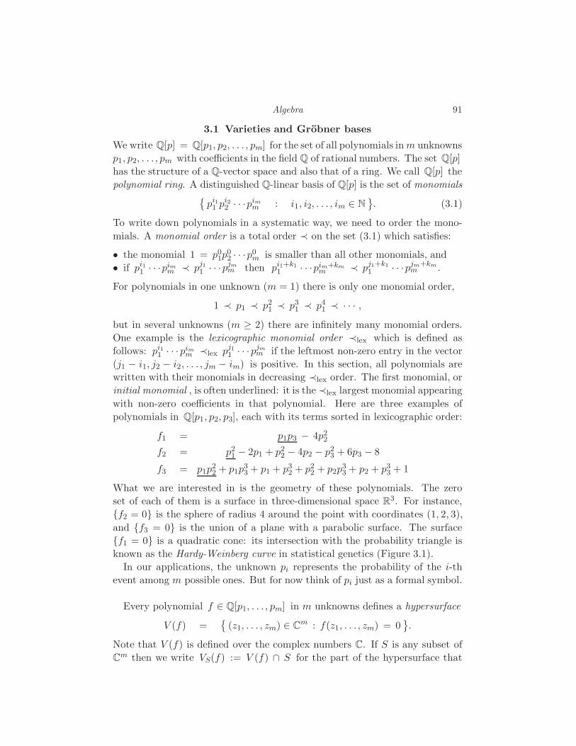
Algebra 91
3.1 Varieties and Grobner bases
We write Q[p] = Q[p1, p2, . . . , pm] for the set of all polynomials inm unknowns
p1, p2, . . . , pm with coefficients in the field Q of rational numbers. The set Q[p]
has the structure of a Q-vector space and also that of a ring. We call Q[p] the
polynomial ring. A distinguished Q-linear basis of Q[p] is the set of monomialspi11 p
i22 · · ·pim
m : i1, i2, . . . , im ∈ N. (3.1)
To write down polynomials in a systematic way, we need to order the mono-
mials. A monomial order is a total order ≺ on the set (3.1) which satisfies:
• the monomial 1 = p01p
02 · · ·p0
m is smaller than all other monomials, and
• if pi11 · · ·pim
m ≺ pj11 · · ·pjm
m then pi1+k11 · · ·pim+km
m ≺ pj1+k11 · · ·pjm+km
m .
For polynomials in one unknown (m = 1) there is only one monomial order,
1 ≺ p1 ≺ p21 ≺ p3
1 ≺ p41 ≺ · · · ,
but in several unknowns (m ≥ 2) there are infinitely many monomial orders.
One example is the lexicographic monomial order ≺lex which is defined as
follows: pi11 · · ·pim
m ≺lex pj11 · · ·pjm
m if the leftmost non-zero entry in the vector
(j1 − i1, j2 − i2, . . . , jm − im) is positive. In this section, all polynomials are
written with their monomials in decreasing ≺lex order. The first monomial, or
initial monomial , is often underlined: it is the ≺lex largest monomial appearing
with non-zero coefficients in that polynomial. Here are three examples of
polynomials in Q[p1, p2, p3], each with its terms sorted in lexicographic order:
f1 = p1p3 − 4p22
f2 = p21 − 2p1 + p2
2 − 4p2 − p23 + 6p3 − 8
f3 = p1p22 + p1p
33 + p1 + p3
2 + p22 + p2p
33 + p2 + p3
3 + 1
What we are interested in is the geometry of these polynomials. The zero
set of each of them is a surface in three-dimensional space R3. For instance,
f2 = 0 is the sphere of radius 4 around the point with coordinates (1, 2, 3),
and f3 = 0 is the union of a plane with a parabolic surface. The surface
f1 = 0 is a quadratic cone: its intersection with the probability triangle is
known as the Hardy-Weinberg curve in statistical genetics (Figure 3.1).
In our applications, the unknown pi represents the probability of the i-th
event among m possible ones. But for now think of pi just as a formal symbol.
Every polynomial f ∈ Q[p1, . . . , pm] in m unknowns defines a hypersurface
V (f) =
(z1, . . . , zm) ∈ Cm : f(z1, . . . , zm) = 0.
Note that V (f) is defined over the complex numbers C. If S is any subset of
Cm then we write VS(f) := V (f) ∩ S for the part of the hypersurface that
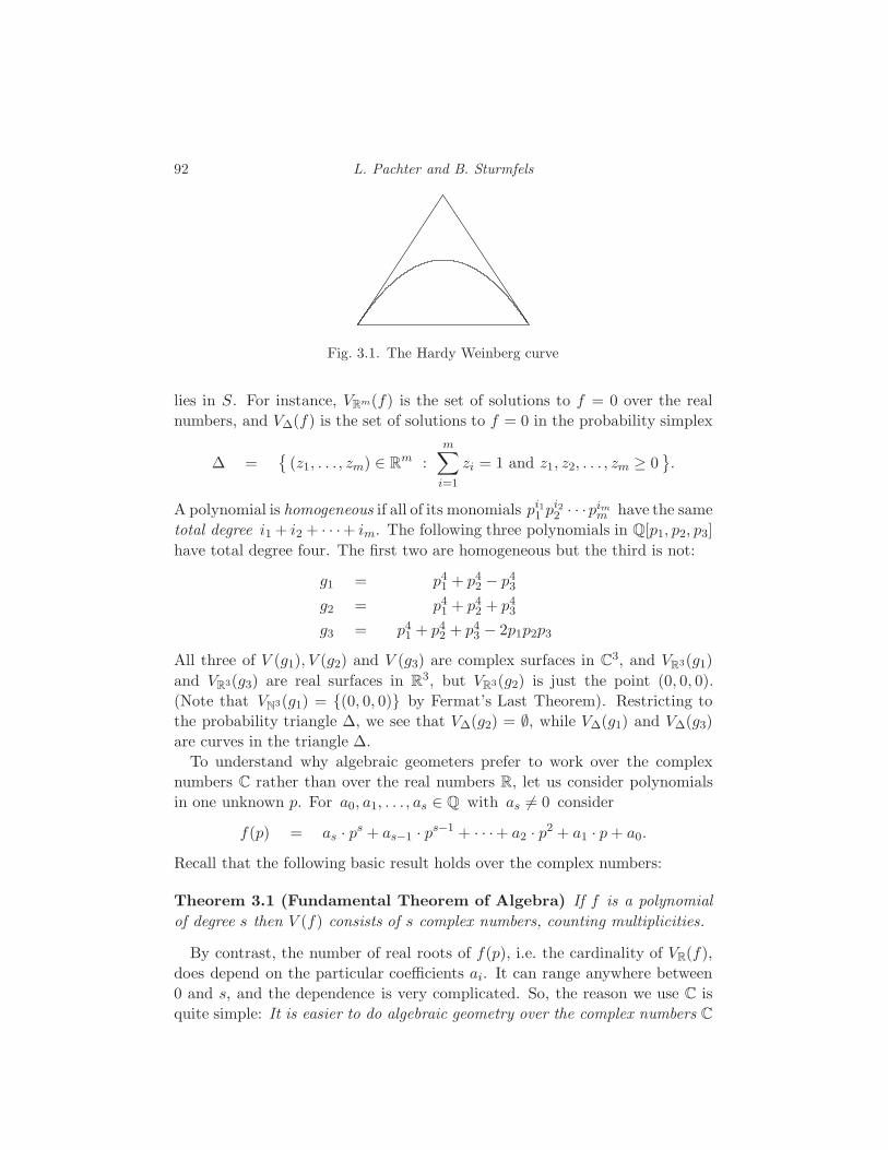
92 L. Pachter and B. Sturmfels
Fig. 3.1. The Hardy Weinberg curve
lies in S. For instance, VRm(f) is the set of solutions to f = 0 over the real
numbers, and V∆(f) is the set of solutions to f = 0 in the probability simplex
∆ =
(z1, . . . , zm) ∈ Rm :
m∑
i=1
zi = 1 and z1, z2, . . . , zm ≥ 0.
A polynomial is homogeneous if all of its monomials pi11 p
i22 · · ·pim
m have the same
total degree i1 + i2 + · · ·+ im. The following three polynomials in Q[p1, p2, p3]
have total degree four. The first two are homogeneous but the third is not:
g1 = p41 + p4
2 − p43
g2 = p41 + p4
2 + p43
g3 = p41 + p4
2 + p43 − 2p1p2p3
All three of V (g1), V (g2) and V (g3) are complex surfaces in C3, and VR3(g1)
and VR3(g3) are real surfaces in R3, but VR3(g2) is just the point (0, 0, 0).
(Note that VN3(g1) = (0, 0, 0) by Fermat’s Last Theorem). Restricting to
the probability triangle ∆, we see that V∆(g2) = ∅, while V∆(g1) and V∆(g3)
are curves in the triangle ∆.
To understand why algebraic geometers prefer to work over the complex
numbers C rather than over the real numbers R, let us consider polynomials
in one unknown p. For a0, a1, . . . , as ∈ Q with as 6= 0 consider
f(p) = as · ps + as−1 · ps−1 + · · ·+ a2 · p2 + a1 · p+ a0.
Recall that the following basic result holds over the complex numbers:
Theorem 3.1 (Fundamental Theorem of Algebra) If f is a polynomial
of degree s then V (f) consists of s complex numbers, counting multiplicities.
By contrast, the number of real roots of f(p), i.e. the cardinality of VR(f),
does depend on the particular coefficients ai. It can range anywhere between
0 and s, and the dependence is very complicated. So, the reason we use C is
quite simple: It is easier to do algebraic geometry over the complex numbers C
Algebra 93
than over the real numbers R. In algebraic statistics, we postpone issues of real
numbers and inequalities as long as we can get away with it. But of course,
at the end of the day, we are dealing with parameters and probabilities, and
those are real numbers which are constrained by inequalities.
Let F be an arbitrary subset of the polynomial ring Q[p1, . . . , pm]. We define
its variety V (F ) as the intersection of the hypersurfaces V (f) where f ranges
over F . Similarly, VS(F ) = ∩f∈FVS(f) for any subset S ⊂ Cm. Using the
example above, the variety V (g1, g3) is a curve in three-dimensional space
C3. That curve meets the probability triangle ∆ in precisely two points:
V∆(g1, g3) = (0.41167, 0.17346, 0.41487), (0.17346, 0.41167, 0.41487) (3.2)
These two points are found by first computing the variety V( g1, g3, p1+p2+
p3−1 ). We did this by running the following sequence of six commands in the
computer algebra package Singular. See Section 2.5 for software references.
ring R = 0, (p1,p2,p3), lp;
ideal I = (p1^4+p2^4-p3^4,p1^4+p2^4+p3^4-2*p1*p2*p3,p1+p2+p3-1);
ideal G = groebner(I); G; LIB ‘‘solve.lib’’; solve(G,10);
For an explanation of these commands, and a discussion of how to solve poly-
nomial systems in general, see Section 2.5 of [Sturmfels, 2002]. Running this
Singular code shows that V( g1, g3, p1 +p2 +p3−1
)consists of 16 distinct
points (which is consistent with Bezout’s Theorem [Cox et al., 1997]). Only
two of the 16 points have all their coordinates real. They lie in the triangle ∆.
Algebraists feel notoriously uneasy about floating point numbers. For a
specific numerical example consider the common third coordinate of the two
points in V∆(g1, g3). When an algebraist sees the floating point number
p3 = 0.4148730882..., (3.3)
(s)he will want to know whether p3 can be expressed in terms of radicals.
Indeed, the floating point coordinates produced by the algorithms in this
book are usually algebraic numbers. An algebraic number has a degree which
is the degree of its minimal polynomial over Q. For instance, our floating point
number p3 is an algebraic number of degree six. Its minimal polynomial equals
f(p3) = 2 · p63 − 4 · p5
3 + 8 · p43 − 8 · p3
3 + 6 · p23 − 4 · p3 + 1.
This polynomial appears in the output of the command line G; in our
Singular program. Most algebraists would probably prefer the following de-
scription (3.4) of our number over the description given earlier in (3.3):
p3 = the smaller of the two real roots of the polynomial f(p3). (3.4)
94 L. Pachter and B. Sturmfels
The other real root is 0.7845389895 but this does not appear in V∆(g1, g3).Our number p3 cannot be written in terms of radicals over Q. This is because
the Galois group of the polynomial f(p3) is the symmetric group on six letters,
which is not a solvable group. To see this, run the following in Maple:
galois( 2*p3^6-4*p3^5+8*p3^4-8*p3^3+6*p3^2-4*p3+1, p3);
In summary, algorithms used in algebraic statistics produce floating numbers,
and these numbers are often algebraic numbers, which means they have a well-
defined algebraic degree over Q. In algebraic statistics, we are sensitive to this
intrinsic measure of complexity of the real numbers we are dealing with.
The command ideal G = groebner(I); in our Singular code computes
the lexicographic Grobner basis for the ideal generated by the three given
polynomials. In what follows, we give a very brief introduction to these notions.
For further details, the reader is referred to any of the numerous textbooks on
computational algebraic geometry which have appeared in the last decade.
Let F ⊂ Q[p] = Q[p1, . . . , pm]. The ideal generated by F is the set 〈F〉 con-
sisting of all polynomial linear combinations of the elements in F . In symbols,
〈F〉 =h1f1 + · · ·+ hrfr : f1, . . . , fr ∈ F and h1, . . . , hr ∈ Q[p]
.
An ideal I in Q[p] is any set of the form I = 〈F〉. It is quite possible for two
different subsets F and F ′ of Q[p] to generate the same ideal I , i.e.,
〈 F 〉 = 〈 F ′ 〉.This equation means that every polynomial in F is a Q[p]-linear combination
of elements in F ′, and vice versa. If this holds then the two varieties coincide:
V (F ) = V (F ′).Hilbert’s basis theorem implies that every variety is the intersection of finitely
many hypersurfaces:
Theorem 3.2 (Hilbert’s basis theorem) Every infinite set F of polyno-
mials in Q[p] has a finite subset F ′ ⊂ F such that 〈 F 〉 = 〈 F ′ 〉.
The theorem is often stated in the following form:
Every ideal in a polynomial ring is finitely generated.
Let us now fix a term order ≺. Every polynomial f ∈ Q[p] has a unique
initial monomial denoted in≺(f). The initial monomial of f is the ≺-largest
monomial pa = pa11 p
a22 · · ·pam
m which appears with non-zero coefficient in the
expansion of f . Let I be an ideal in Q[p]. Then its initial ideal in≺(I) is the
ideal generated by the initial monomials of all the polynomials in I :
in≺(I) := 〈 in≺(f) : f ∈ I 〉.
Algebra 95
A finite subset G of an ideal I is a Grobner basis with respect to the monomial
order ≺ if the initial monomials of elements in G generate the initial ideal:
in≺(I) = 〈 in≺(g) : g ∈ G 〉. (3.5)
As we have defined it in (3.5), there is no minimality requirement for being
a Grobner basis. If G is a Grobner basis for I then we can augment G by any
additional elements from I and the resulting set is still a Grobner basis. To
remedy this non-minimality, we make one more definition. We say that G is a
reduced Grobner basis if the following three additional conditions hold:
(i) For each g ∈ G, the coefficient of in≺(g) in g is 1.
(ii) The set in≺(g) : g ∈ G minimally generates in≺(I).
(iii) No trailing term of any g ∈ G lies in in≺(I).
For a fixed term order ≺, every ideal I in Q[p1, . . . , pm] has a unique reduced
Grobner basis G. This reduced Grobner basis is finite, and it can be computed
from an arbitrary generating set F of I by the so-called Buchberger algorithm.
Any Grobner basis generates the ideal for which it is a Grobner basis, so in
particular, the reduced Grobner basis satisfies 〈G〉 = 〈F〉 = I.
We will discuss the Buchberger algorithm towards the end of this section.
First, we concentrate on some applications to the study of algebraic varieties.
Recall that varieties are the solution sets of polynomial equations in several
unknowns. Here we take polynomials with rational coefficients, and we consider
a finite set of them F ⊂ Q[p1, . . . , pm]. The variety of F is the set of all common
zeros of F over the field of complex numbers. As above it is denoted
V(F ) =
(z1, . . . , zm) ∈ Cm : f(z1, . . . , zm) = 0 for all f ∈ F.
The variety does not change if we replace F by another set of polynomials that
generates the same ideal in Q[p1, . . . , pm]. In particular, the reduced Grobner
basis G for the ideal 〈F〉 specifies the same variety:
V(F ) = V(〈F〉) = V(〈G〉) = V(G).
The advantage of G is that it reveals geometric properties of the variety which
are not visible from the given polynomials F . A most basic question which
one might ask about the variety V (F ) is whether it is non-empty: does the
given system of equations F have any solution over the complex numbers?
Theorem 3.3 (Hilbert’s Nullstellensatz) The variety V (F ) is empty if
and only if the reduced Grobner basis G of the ideal 〈F〉 equals 1.
Example 3.4 Consider a set of three polynomials in two unknowns:
F = θ21 + θ1θ2 − 10, θ31 + θ1θ22 − 25, θ41 + θ1θ
32 − 70 .

96 L. Pachter and B. Sturmfels
Running the Buchberger algorithm on the input F , we find that G = 1,so the three given polynomials have no common zero (θ1, θ2) in C2. We now
change the constant term of the middle polynomial as follows:
F = θ21 + θ1θ2 − 10, θ31 + θ1θ22 − 26, θ41 + θ1θ
32 − 70 .
The reduced Grobner basis of 〈F〉 is G = θ1−2, θ2−3 . This shows that the
variety of F consists of a single point in C2, namely, V(F ) = V(G) = (2, 3) .
Our next question is how many zeros does a given system of equations
have ? To answer this we need one more definition. Given a fixed ideal I
in Q[p1, . . . , pm] and a fixed term order ≺, a monomial pa = pa11 · · ·pam
m is
called standard if it is not in the initial ideal in≺(I). The number of standard
monomials is finite if and only if every unknown pi appears to some power
among the generators of the initial ideal. For example, if in≺(I) = 〈 p31, p
42, p
53 〉
then there are 60 standard monomials, but if in≺(I) = 〈 p31, p
42, p1p
43 〉 then the
set of standard monomials is infinite (because every power of p3 is standard).
Theorem 3.5 The variety V(I) is finite if and only if the set of standard
monomials is finite. In this case, the number of standard monomials equals
the cardinality of V(I), when zeros are counted with multiplicity.
In the case of one unknown p, this result is the Fundamental Theorem of
Algebra (Theorem 3.1), which states that the variety V(f) of a polynomial
f ∈ Q[p] of degree s consists of s complex numbers. Indeed, in this case fis a Grobner basis for its ideal I = 〈f〉, we have in≺(I) = 〈ps〉, and there
are precisely s standard monomials: 1, p, p2, . . . , ps−1. Thus we can regard
Theorem 3.5 as the Multidimensional Fundamental Theorem of Algebra.
Example 3.6 Consider the system of three polynomials in three unknowns
F =p41 + p4
2 − p43 , p
41 + p4
2 + p43 − 2p1p2p3 , p1 + p2 + p3 − 1
Its Grobner basis for the purely lexicographic order p1 > p2 > p3 equals
G =p1 + p2 + p3 − 1 , p2
2p3 + p2p23 − p2p3 + p4
3, 2p73 − 4p6
3 + 8p53 + · · · ,
2p42 + 4p3
2p3 − 4p32 + 6p2
2p23 − 10p2
2p3 + 6p22 + 4p2p
33 − 10p2p
23+ · · ·
.
The underlined initial monomials show that there are 16 standard monomials:
1, p2, p22, p
32, p3, p
23, p
33, p
43, p
53, p
63, p2p3, p2p
23, p2p
33, p2p
43, p2p
53, p2p
63.
Theorem 3.5 says V (F ) consists of 16 points. Two of them appear in (3.2).
Our criterion in Theorem 3.5 for deciding whether a variety is finite general-
izes to the following formula for the dimension of a variety. A subset S of the
Algebra 97
set of unknowns p1, p2, . . . , pm is a standard set if every monomial∏
pj∈S paj
j
in those unknowns is standard. Equivalently, in≺(I) ∩ C[ pj : j ∈ S ] = 0.
Theorem 3.7 (Dimension Formula) The dimension of an algebraic vari-
ety V(I) ⊂ Cm is the maximal cardinality of any standard set for the ideal I.
For a proof of this combinatorial dimension formula, and many other basic
results on Grobner basis, we refer to [Cox et al., 1997].
Example 3.8 Let I ⊂ Q[p1, p2, p3] be the ideal generated by the Hardy-
Weinberg polynomial f1 = p1p3 − 4p22. The maximal standard sets for I in the
lexicographic monomial order are p1, p2 and p2, p3. Both have cardinality
two. Hence the variety V (f1) has dimension two: it is a surface in C3.
Another basic result states that the set of standard monomials is a Q-vector
space basis for the residue ring Q[p1, . . . , pm]/I . The image of any polynomial
h in this residue ring can be expressed uniquely as a Q-linear combination
of standard monomials. This expression is the normal form of h modulo the
Grobner basis G. The process of computing the normal form is the division
algorithm. In the case of one unknown p, where I = 〈f〉 and f has degree s, the
division algorithm writes any polynomial h ∈ Q[p] as a unique Q-linear com-
bination of the standard monomials 1, p, p2, . . . , ps−1. The division algorithm
works relative to a Grobner basis in any number m of unknowns.
Example 3.9 Let Q[p] be the polynomial ring in 16 unknowns, denoted
p =
pAA pAC pAG pATpCA pCC pCG pCTpGA pGC pGG pGTpTA pTC pTG pTT
DiaNA’s model in Example 1.16 for generating two DNA sequences is
pij = π · λ1i · λ2
j + (1− π) · ρ1i · ρ2
j where i, j ∈ A, C, G, T. (3.6)
Since “statistical models are algebraic varieties”, this model can be represented
as a variety V (I) in C4×4. The homogeneous ideal I ⊂ Q[p] corresponding to
the model (3.6) is generated by the sixteen 3× 3-minors of the 4× 4-matrix p.
These sixteen determinants form a reduced Grobner basis for I :
G =pAApCCpGG − pAApCGpGC − pACpCApGG + pACpCGpGA + pAGpCApGC − pAGpCCpGA,
pAApCCpGT − pAApCTpGC − pACpCApGT + pACpCTpGA + pATpCApGC − pATpCCpGA,
· · · · · · · · · · · · · · · · · · · · · · · · · · ·pCCpGGpTT − pCCpGTpTG − pCGpGCpTT + pCGpGTpTC + pCTpGCpTG − pCTpGGpTC
.
98 L. Pachter and B. Sturmfels
Indeed, it is known [Sturmfels, 1990] that, for any a, b, c ∈ N, the a× a-minors
of a b × c-matrix of unknowns form a reduced Grobner basis with respect to
a term order that makes the main diagonal terms of any determinant highest.
We are looking at the case a = 3, b = c = 4. The variety V (G) = V (I) consists
of all complex 4 × 4-matrices of rank ≤ 2. We can compute the dimension of
this variety using Theorem 3.7. There are twenty maximal standard sets for
I . They all have cardinality 12. One such standard set is
S =pAA, pAC, pAG, pAT , pCA, pCC, pCG, pCT , pGA, pGC , pTA, pTC
.
Indeed, none of the monomials in these twelve unknowns lie in the initial ideal
in≺(I) =⟨pAApCCpGG , pAApCCpGT , pAApCGpGT , . . . , pCCpGGpTT
⟩.
Theorem 3.7 implies that the variety V (I) has dimension |S| = 12, and its
intersection with the probability simplex, V∆(I), has dimension 11.
To illustrate the division algorithm, we consider the non-standard monomial
h = pAA · pCC · pGG · pTTThe normal form of hmodulo G is the following sum of 12 standard monomials:
nfG(h) = pAApCTpGGpTC + pACpCApGTpTG − pACpCTpGGpTA + pAGpCCpGApTT
−pAGpCCpGTpTA − pAGpCTpGApTC + pAGpCTpGCpTA − pATpCApGGpTC
−pATpCCpGApTG + pATpCGpGApTC − pATpCGpGCpTA + 2 · pATpCCpGGpTAWe have h ≡ nfG(h) for all probability distributions as in (3.6).
Our assertion in Example 3.9 that the 3 × 3-minors form a Grobner basis
raises the following question. Given a fixed term order ≺, how can one test
whether a given set of polynomials G is a Grobner basis or not? The answer is
given by the following criterion [Buchberger, 1965]. Consider any two polyno-
mials g and g′ in G and form their S-polynomial m′g−mg′. Here m and m′ are
monomials of smallest possible degree such that m′ · in≺(g) = m · in≺(g′). The
S-polynomial m′g−mg′ lies in the ideal 〈G〉. We apply the division algorithm
modulo the tentative Grobner basis G to the input m′g −mg′. The resulting
normal form nfG(m′g −mg′) is a Q-linear combination of monomials none of
which is divisible by an initial monomial from G. A necessary condition for Gto be a Grobner basis is that this result be zero:
nfG(m′g −mg′) = 0 for all g, g′ ∈ G. (3.7)
Theorem 3.10 (Buchberger’s Criterion) A finite set of polynomials G ⊂Q[p1, . . . , pm] is a Grobner basis for its ideal 〈G〉 if and only if (3.7) holds,
that is, if and only if all S-polynomials have normal form zero.

Algebra 99
So, to check that the set G of the sixteen 3× 3-determinants in Example 3.9
is indeed a Grobner basis, it suffices to compute the normal forms of all(16
2
)
pairwise S-polynomials, such as
pTG · (pAApCCpGG − pAApCGpGC − · · · ) − pGG · (pAApCCpTG − pAApCGpTC − · · · )
= −pAApCGpGCpTG + pAApCGpGGpTC + pACpCGpGApTG − pACpCGpGGpTA
+pAGpCApGCpTG − pAGpCApGGpTC − pAGpCCpGApTG + pAGpCCpGGpTA
The normal form of this expression modulo G is zero, as promised.
We are now prepared to state the algorithm for computing Grobner bases.
Algorithm 3.11 (Buchberger’s Algorithm)
Input: A finite set F of polynomials in Q[p1, p2, . . . , pm] and a term order ≺.
Output: The reduced Grobner basis G of the ideal 〈F〉 with respect to ≺.
Step 1: Apply Buchberger’s Criterion to see whether F is already a Grobner
basis. If yes go to Step 3.
Step 2: If no, we found a non-zero polynomial nfG(m′g −mg′). Enlarge the
set F by adding this non-zero polynomial and go back to Step 1.
Step 3: Transform the Grobner basis F to a reduced Grobner basis G.
This loop between Steps 1 and 2 will terminate after finitely many iterations
because at each stage the ideal generated by the current initial monomials get
strictly bigger. However, in light of Hilbert’s Basis Theorem, every strictly
increasing sequence of ideals Q[p1, . . . , pm] must stabilize eventually.
The Grobner basis F produced in Steps 1 & 2 is usually not reduced, so in
Step 3 we perform auto-reduction to make F reduced. To achieve the three
conditions in the definition of reduced Grobner basis, here is what Step 3 does.
First, each polynomial in F is divided by its leading coefficient to achieve
condition 1. Next, one removes redundant polynomials to achieve condition 2.
Finally, each polynomial is replaced by its normal form with respect to F to
achieve condition 3. The resulting set G satisfies all three conditions.
We illustrate Buchberger’s algorithm for a very simple example with m = 1:
F =p2 + 3p− 4, p3 − 5p+ 4
.
This set is not a Grobner basis because the S-polynomial
p · (p2 + 3p− 4)− 1 · (p3 − 5p+ 4) = 3p2 + p− 4
has the non-zero normal form
3p2 + p− 4 − 3 · (p2 + 3p− 4) = −8p+ 8.
The new set F ∪ −8p + 8 now passes the test imposed by Buchberger’s
Criterion: it is a Grobner basis. The resulting reduced Grobner basis equals
G = p− 1 . In particular, we conclude V (F ) = 1 ⊂ C.
100 L. Pachter and B. Sturmfels
Remark 3.12 If F ⊂ Q[p] is a set of polynomials in one unknown p then the
reduced Grobner basis G of the ideal 〈F〉 consists of only one polynomial g.
The polynomial g is the greatest common divisor of F .
Buchberger’s algorithm is therefore a generalization of the Euclidean algo-
rithm for polynomials in one unknown. Likewise, the Buchberger Algorithm
simulates Gaussian elimination if we apply it to a set F of linear polynomials.
We can thus think of Grobner bases as a Euclidean algorithm for multivariate
polynomials or a Gaussian elimination for non-linear equations.
In summary, Grobner bases and the Buchberger Algorithm for finding them
are fundamental notions in computational algebra. They also furnish the en-
gine for more advanced algorithms for algebraic varieties. Polynomial models
are ubiquitous across the sciences, and play a role in numerous biological con-
texts, including settings quite different from those described in this book. For
example, they are used in computational systems biology [Laubenbacher, 2003]
and for finding equilibria in reaction networks [Craciun and Feinberg, 2004,
Gatermann and Wolfrum, 2005]. Computer programs for algebraic geometry
include CoCoA, Macaulay 2 and Singular. All three are free and easy to use.
Within minutes you will be able to test whether a variety V(F ) is empty, and,
if not, compute its dimension.
3.2 Implicitization
Consider the polynomial map which represents an algebraic statistical model:
f : Cd → Cm. (3.8)
Here the ambient spaces are taken over the complex numbers, but the coordi-
nates f1, . . . , fm of the map f are polynomials with rational coefficients, i.e.,
f1, . . . , fm ∈ Q[θ1, . . . , θd]. These assumptions are consistent with our discus-
sion in the previous section. We start out by investigating the following basic
question: is the image of a polynomial map f really an algebraic variety?
Example 3.13 Consider the following map from the plane into three-space:
f : C2 → C3 , (θ1, θ2) 7→(θ21, θ1 · θ2, θ1 · θ2
)
The image of f is a dense subset of a plane in three-space, namely, it is
f(C2) =
(p1, p2, p3) ∈ C3 : p2 = p3 and ( p1 = 0 implies p2 = 0 )
=(V (p2 − p3) \ V (p1, p2 − p3)
)∪ V (p1, p2, p3).
Thus the image of f is not an algebraic variety, but its closure is: f(C2) =
V (p2 − p3). The set f(C2) is a Boolean combination of algebraic varieties.
Algebra 101
The following general theorem holds in algebraic geometry. It can be derived
from the Closure Theorem in Section 3.2 of [Cox et al., 1997].
Theorem 3.14 The image of a polynomial map f : Cd → Cm is a Boolean
combination of algebraic varieties in Cm. The topological closure f(Cd) of the
image f(Cd) in Cm is an algebraic variety.
The statements in this theorem are not true if we replace the complex num-
bers C by the real numbers R. This can already be seen for the map f in
Example 3.13. The image of this map over the reals equals
f(R2) =
(p1, p2, p3) ∈ R3 : p2 = p3 and ( p1 > 0 or p1 = p2 = p3 = 0 ).
The closure of the image is a half-plane in R3, which is not an algebraic variety:
f(R2) =
(p1, p2, p3) ∈ R3 : p2 = p3 and p1 ≥ 0.
It is instructive to carry this example a little further and compute the images
of various subsets Θ of R2. For instance, what is the image f(Θ) of the
square Θ = 0 ≤ θ1, θ2 ≤ 1? For answering such questions in general, we
need algorithms for solving polynomial inequalities over the real numbers. Such
algorithms exists in real algebraic geometry, which is an active area of research.
However, real algebraic geometry lies beyond what we are hoping to explain
in this book. In this chapter, we restrict ourselves to the much simpler setting
of polynomial equations over the complex numbers. For an introduction to
algorithms in real algebraic geometry see [Basu et al., 2003].
We shall adopt the following convention: By the image of the polynomial map
f in (3.8) we shall mean the algebraic variety f(Cd) in Cm. Thus we disregard
potential points p in f(Cd)\f(Cd). This is not to say they are not important.
In fact, in a statistical model for a biological problem, such boundary points p
might represent probability distributions we really care about. If so, we need
to refine our techniques. For the discussion in this chapter, however, we keep
the algebra as simple as possible and refer to f(Cd) as the image of f .
Let If denote the set of all polynomials in Q[p1, . . . , pm] that vanish on the set
f(Cd). Thus If is the ideal which represents the variety f(Cd). A polynomial
h ∈ Q[p1, . . . , pm] lies in the ideal If if and only if
h(f1(t), f2(t), . . . fm(t)
)= 0 for all t = (t1, t2, . . . , td) ∈ Rd. (3.9)
The ideal If is a prime ideal. This means that if a factorizable polynomial
h = h′ · h′′ satisfies (3.9) then one of its factors h′ or h′′ will also satisfy (3.9).
In the condition (3.9) we can replace Rd by any open subset Θ ⊂ Rd and we get
an equivalent condition. Thus If equals the set of all polynomials that vanish
on the points f(t) where t runs over the parameter space Θ. The polynomials
in the prime ideal If are known as model invariants in algebraic statistics. For

102 L. Pachter and B. Sturmfels
instance, for DiaNA’s model in Example 3.9, the model invariants include the
3 × 3-minors of the 4 × 4-matrix of probabilities.
The computational task resulting from our discussion is called implicitiza-
tion: Given m polynomials f1, . . . , fm in Q[θ1, . . . , θd] which represent a poly-
nomial map f : Cd → Cm, implicitization seeks to compute a finite set F of
polynomials in Q[p1, p2, . . . , pm] such that 〈F〉 = If . Actually, it would be
preferable to have a Grobner basis G of the ideal If . Our point of view is this:
“compute the image of a polynomial map f
means “compute generators of the prime ideal If”
Example 3.15 We compute the images of five different maps f : C2 → C3:
(a) If f = ( θ21, θ1θ2, θ1θ2 ) then If = 〈 p2 − p3 〉. This is Example 3.13.
(b) If f = ( θ21, 2θ1θ2, θ22 ) then If = 〈 p1p3 − 4p2
2 〉 = Hardy-Weinberg.
(c) If f = ( θ51, θ1θ2, θ42 ) then If = 〈 p4
1p53 − p20
2 〉.(d) If f = ( θ51 +θ1θ2, θ
51 +θ42 , θ1θ2 +θ42 ) then we get the same ideal in new
coordinates: If = 〈 211(p1 +p2 −p3)4(p2 +p3 −p1)
5− (p1 +p3 −p2)20 〉.
(e) If f = ( θ21 + θ22 , θ31 + θ32, θ
41 + θ42 ) then we actually have to do a com-
putation to find If = 〈 p61 − 4p3
1p22 − 4p4
2 + 12p1p22p3 − 3p2
1p23 − 2p3
3 〉.
The last ideal If was computed in Singular using the following six commands:
ring s=0, (p1,p2,p3),lp;
ring r=0, (t1,t2), lp;
map f = s, t1^2+t2^2, t1^3+t2^3, t1^4+t2^4;
ideal i0 = 0;
setring s;
preimage(r,f,i0);
It should be tried and then redone with the third line replaced as follows:
map f = s, t1^5+t1*t2, t1^5+t2^4, t1*t2+t2^4;
This produces the surface of degree 20 in Example 3.15 (d). The output is
very large, and underlines the importance of identifying a coordinate change
that will simplify a computation. This will be crucial for the applications to
phylogenetics discussed in Chapter 15 and 16.
In order to understand the way Grobner basis software (such as Singular)
computes images of polynomial maps, we need to think about the ideal If in
the following algebraic manner. Our polynomial map f : Cd → Cm induces
the map between polynomial rings in the opposite direction:
f∗ : Q[p1, p2, . . . , pm] → Q[θ1, . . . , θd]
h(p1, p2, . . . , pm) 7→ h(f1(θ), f2(θ), . . . , fm(θ))
Algebra 103
The map f∗ is a ring homomorphism, which means that f∗(h′+h′′) = f∗(h′)+
f∗(h′′) and f∗(h′·h′′) = f∗(h′)·f∗(h′′). Thus the ring homomorphism is uniquely
specified by saying that f∗(pi) = fi(θ) for all i. The kernel of f∗ is the set
(f∗)−1(0) of all polynomials h ∈ Q[p1, . . . , pm] that get mapped to zero by f∗.
Proposition 3.16 The kernel of f∗ equals the prime ideal If ⊂ Q[p1, . . . , pm].
Proof A polynomial h satisfies f∗(h) = 0 if and only if the condition (3.9)
holds. Thus h lies in kernel(f∗) = (f∗)−1(0) if and only if h lies in If .
If I is any ideal in Q[θ1, . . . , θd] then its preimage (f∗)−1(I) is an ideal in
Q[p1, . . . , pm]. The next theorem characterizes the variety in Cm of this ideal.
Theorem 3.17 The variety of (f∗)−1(I) is the closure in Cm of the image of
the variety V (I) ⊂ Cd under the map f ; in symbols,
V((f∗)−1(I)
)= f
(V (I) ) ⊂ Cm. (3.10)
Proof We identify the ideal I with its image in the enlarged polynomial ring
Q[θ1, . . . θd, p1, p2, . . . , pm]. Inside this big polynomial ring we consider the ideal
J = I + 〈 p1 − f1(θ), p2 − f2(θ), . . . , pm − fm(θ) 〉. (3.11)
The ideal J represents the graph of the restricted map f : V (I) → Cm. Indeed,
that graph is precisely the variety V (J) ⊂ Cd+m. The desired image f(V (I))
is obtained by projecting the graph V (J) onto the space Cm with coordinates
p1, . . . , pm. Algebraically, this corresponds to computing the elimination ideal
(f∗)−1(I) = J ∩ Q[p1, . . . , pm]. (3.12)
Now use the Closure Theorem in [Cox et al., 1997, Sect. 3.2].
The Singular code displayed earlier is designed for the setup in (3.10). The
map command specifies a homomorphism f from the second polynomial ring
s to the first polynomial ring r, and the preimage command computes the
preimage of an ideal i0 in r under the homomorphism f. The computation
inside Singular is done by cleverly executing the two steps (3.11) and (3.12).
Example 3.18 We compute the image of the hyperbola V (θ1θ2 − 1) under
the map f in Example 3.15 (e) by replacing the line ideal i0 = 0 ; by the
new line ideal i0 = t1*t2-1 ; in our code. The image of the hyperbola
in three-space is a curve which is the intersection of two quadratic surfaces:
(f∗)−1(〈θ1θ2−1〉
)= 〈 p1p3−p1−p2
2+2 , p21−p3−2 〉 ⊂ Q[p1, p2, p3]

104 L. Pachter and B. Sturmfels
Example 3.19 Consider the hidden Markov model of Subsection 1.4.3 where
n = 3 and both the hidden and observed states are binary (l = l′ = 2). The
parameterization (1.52) is a map f : R4 → R8 which we enter into Singular:
ring s = 0, (p000, p001, p010, p011, p100, p101, p110, p111),lp;
ring r = 0, ( x,y, u,v ), lp;
map f = s, x^2*u^3 + x*(1-x)*u^2*(1-v) +
(1-x)*(1-y)*u^2*(1-v) + (1-x)*y*u*(1-v)^2 + (1-y)*x*(1-v)*u^2 +
(1-y)*(1-x)*(1-v)^2*u + y*(1-y)*(1-v)^2*u + y^2*(1-v)^3,
x^2*u^2*(1-u) + x*(1-x)*u^2*v + (1-x)*(1-y)*u*(1-v)*(1-u) +
(1-x)*y*u*(1-v)*v + (1-y)*x*(1-v)*u*(1-u) +
(1-y)*(1-x)*(1-v)*u*v + y*(1-y)*(1-v)^2*(1-u) + y^2*(1-v)^2*v,
x^2*u^2*(1-u) + x*(1-x)*u*(1-u)*(1-v) + (1-x)*(1-y)*u^2*v +
(1-x)*y*u*(1-v)*v + (1-y)*x*(1-v)*u*(1-u) +
(1-y)*(1-x)*(1-v)^2*(1-u) + y*(1-y)*(1-v)*v*u +y^2*(1-v)^2*v,
x^2*u*(1-u)^2 + x*(1-x)*u*(1-u)*v + (1-x)*(1-y)*u*v*(1-u) +
(1-x)*y*u*v^2 + (1-y)*x*(1-v)*(1-u)^2 + y^2*(1-v)*v^2 +
(1-y)*(1-x)*(1-v)*(1-u)*v + y*(1-y)*(1-v)*v*(1-u),
x^2*u^2*(1-u) + x*(1-x)*u*(1-u)*(1-v) +
(1-x)*(1-y)*u*(1-v)*(1-u) + (1-x)*y*(1-u)*(1-v)^2 +
(1-y)*x*v*u^2 + (1-y)*(1-x)*(1-v)*u*v + y*(1-y)*(1-v)*v*u +
y^2*(1-v)^2*v, x^2*u*(1-u)^2 + x*(1-x)*u*(1-u)*v +
(1-x)*(1-y)*(1-u)^2*(1-v) + (1-x)*y*(1-u)*(1-v)*v +
(1-y)*x*v*u*(1-u) + (1-y)*(1-x)*v^2*u + y*(1-y)*(1-v)*v*(1-u) +
y^2*(1-v)*v^2, x^2*u*(1-u)^2 + x*(1-x)*(1-u)^2*(1-v) +
(1-x)*(1-y)*u*v*(1-u) + (1-x)*y*(1-u)*(1-v)*v +
(1-y)*x*v*u*(1-u) + (1-y)*(1-x)*(1-v)*(1-u)*v + y*(1-y)*v^2*u +
y^2*(1-v)*v^2, x^2*(1-u)^3 + x*(1-x)*(1-u)^2*v +
(1-x)*(1-y)*(1-u)^2*v + (1-x)*y*(1-u)*v^2 + (1-y)*x*v*(1-u)^2 +
(1-y)*(1-x)*v^2*(1-u) + y*(1-y)*v^2*(1-u) + y^2*v^3;
Here the eight probabilities have been scaled by a factor of two (the initial
distribution is uniform), and the model parameters are abbreviated
θ00 = x , θ01 = 1− x , θ10 = 1 − y , θ11 = y
θ′00 = u , θ′01 = 1 − u , θ′10 = 1 − v , θ′11 = v.
The model invariants of the hidden Markov model can now be computed using
ideal i0 = 0; setring s; preimage(r,f,i0);
This computation will be discussed in Chapter 11. Suppose we are interested
(for some strange reason) in the submodel obtained by equating the transition

Algebra 105
matrix θ with the inverse of the output matrix θ′. The invariants of this
two-dimensional submodel are found by the method of Theorem 3.17, using
ideal i = x*u + x*v - x - v, y*u + y*v - y - u ; setring s;
preimage(r,f,i);
The extension of these computations to longer chains (n ≥ 4) becomes pro-
hibitive. Off-the-shelf implementations in any Grobner basis package will al-
ways run out of steam quickly when the instances get bigger. More specialized
linear algebra techniques need to be employed in order to compute invariants
of larger statistical model. Chapter 11 is devoted to these important issues.
We next discuss an implicitization problem which concerns an algebraic vari-
ety known as the Grassmannian. In our discussion of the space of phylogenetic
trees in Section 3.5, we shall argue that the Grassmannian is a valuable geo-
metric tool for understanding and designing algorithms for biology. Let Q[ θ ]
be the polynomial ring in the unknown entries of the 2 × n matrix
θ =
(θ11 θ12 θ13 . . . θ1n
θ21 θ22 θ23 . . . θ2n
).
Let Q[ p ] =[pij : 1 ≤ i < j ≤ n
]be the polynomial ring in the unknowns
p12, p13, p23, p14, p24, p34, p15, . . . , pn−1,n
. (3.13)
Consider the ring homomorphism f∗ : Q[ p ] → Q[ θ ] , pij 7→ θ1iθ2j − θ1jθ2i.
The corresponding polynomial map f : C2×n 7→ C(n2) takes a 2×n-matrix to
the vector of 2× 2-subdeterminants of θ. The image of this map is the Grass-
mannian, denoted G2,n = f(C2n). The Grassmannian is an algebraic variety,
i.e., it is closed: f(C2n) = f(C2n). The prime ideal of the Grassmannian is
denoted I2,n = kernel(f∗). This ideal has a nice Grobner basis:
Theorem 3.20 The ideal I2,n is generated by the quadratic polynomials
pikpjl − pijpkl − pilpjk (1 ≤ i < j < k < l ≤ n). (3.14)
These form the reduced Grobner basis when the underlined terms are leading.
Proof See Theorem 3.1.7 and Proposition 3.7.4 in [Sturmfels, 1993].
The dimension of the Grassmannian G2,n is computed using Theorem 3.7.
The initial ideal in≺(I2,n) = 〈 pik · pjl : 1 ≤ i < j < k < l ≤ n 〉 can be
visualized as follows. Draw a convex n-gon with vertices labeled 1, 2, 3, . . . , n.
We identify the unknown pij with the line segment connecting the vertex i
106 L. Pachter and B. Sturmfels
and the vertex j. The generators of in≺(I2,n) are the pairs of line segments
that cross each other. Consider an arbitrary monomial in Q[ p ]:
m =∏
(i,j)∈S
paij
ij (where aij > 0 for all (i, j) ∈ S).
This monomial m is standard if and only if m does not lie in in≺(I2,n) if and
only if the set S contains no crossing diagonals if and only if the line segments
in S form a subdivision of the n-gon. Hence a subset S of (3.13) is a maximal
standard set if and only if the edges in S form a triangulation of the n-gon.
The number of triangulations S of the n-gon is the Catalan number 1n+1
(2nn
).
The number of edges in each triangulation S equals |S| = 2n− 3.
Corollary 3.21 The Grassmannian G2,n = V (I2,n) has dimension 2n− 3.
The ideal I2,n is known as the Plucker ideal, and the quadratic polynomials
in (3.14) are known as the Plucker relations. The Plucker ideal I2,n has two
natural generalizations. First, we can replace θ by a d×n-matrix of unknowns
(for any d < n) and we can define the Plucker ideal Id,n by taking the algebraic
relations among the d × d-minors of θ. Thus Id,n is a prime ideal in the
polynomial ring in(nd
)unknowns Q[ p ] = Q
[pi1i2···id : 1 ≤ i1 < i2 < · · · <
id ≤ n]. The corresponding variety in C(n
d) is the Grassmannian Gd,n =
V (Id,n). Regarding Gd,n as projective variety, the points in Gd,n are in a
natural bijection with the d-dimensional linear subspaces of the n-dimensional
vector space Cn. Here p = f(θ) ∈ C(nd) corresponds to the row space of
the matrix θ. Theorem 3.20 generalizes to this situation: the ideal Id,n is
generated by quadratic polynomials known as the Plucker relations. Among
these are the three-term Plucker relations which are derived from (3.14):
pν1···νd−2ik · pν1···νd−2jl − pν1···νd−2ij · pν1···νd−2kl − pν1···νd−2il · pν1···νd−2jk. (3.15)
The three-term Plucker relations are not quite enough to not generate Id,n.
The second natural generalization of the ideal I2,n is based on the identity
(pikpjl − pijpkl − pilpjk
)2= det
0 pij pik pil
−pij 0 pjk pjl
−pik −pjk 0 pkl
−pil −pjl −pkl 0
. (3.16)
This is a skew-symmetric 4 × 4-matrix with unknown entries pij. The square
root of the determinant of a skew-symmetric 2k×2k-matrix is a polynomial of
degree k known as its pfaffian. Hence the Plucker relation (3.14) is the pfaffian
of the matrix in (3.16). Skew-symmetric matrices of odd size are singular, so
the determinant of a skew-symmetric (2k+ 1)× (2k+ 1)-matrix is zero.
Algebra 107
Remark 3.22 By Theorem 3.20 and (3.16), the Plucker ideal I2,n is generated
by the 4×4-subpfaffians of an indeterminate skew-symmetric n×n-matrix (pij).
Let I2,n,k be the ideal generated by the 2k × 2k-subpfaffians of a skew-
symmetric n× n-matrix pij. Thus I2,n,2 = I2,n, and I2,6,3 is generated by
p14p25p36 − p15p24p36p14p26p35 + p15p26p34 − +p16p24p35
p16p25p34 + p13p26p45 − p12p36p45p16p23p45p13p25p46
− + p12p35p46 + p15p23p46 + p13p24p56 − p12p34p56p14p23p56
= det1/2
0 p12 p13 p14 p15 p16
−p12 0 p23 p24 p25 p26
−p13 −p23 0 p34 p35 p36
−p14 −p24 −p34 0 p45 p46
−p15 −p25 −p35 −p45 0 p56
−p16 −p26 −p36 −p46 −p56 0
. (3.17)
It turns out that I2,n,k is always a prime ideal. We introduce k − 1 matrices
θ(s) =
(θ(s)11 θ
(s)12 θ
(s)13 · · · θ
(s)1n
θ(s)21 θ
(s)22 θ
(s)23 · · · θ
(s)2n
)(s = 1, 2, . . . , k− 1).
The 2(k− 1)n entries of these k − 1 matrices are the parameters for the map
g : (C2×n)k−1 → C(n2) , (θ(1), . . . , θ(k−1)) 7→ f(θ(1)) + · · · + f(θ(k−1)). (3.18)
Theorem 3.23 The image of the map g is the variety defined by the 2k×2k-
subpfaffians. We have Ig = I2,n,k and image(g) = V (I2,n,k).
The variety V (I2,n,k) consists of all skew-symmetric n × n-matrices of rank
less than 2k. Geometrically, V (I2,n,k) is the (k − 1)st secant variety of the
Grassmannian. Indeed, the passage from the polynomial map f to the polyno-
mial map g in (3.18) corresponds to the geometric construction of passing from
a projective variety to its (k−1)st secant variety. For a proof of Theorem 3.23
see [De Concini et al., 1982]. The Grobner basis in Theorem 3.20 generalizes
from I2,n to I2,n,k, and so does its convex n-gon interpretation. The initial
ideal in≺(I2,n,k) for a suitable term order ≺ is generated by the k-element
sets of pairwise crossing diagonals (see [Dress et al., 2002]). As an example
consider the 15 monomials in the cubic pfaffian given above (this is the case
k = 3, n = 6). The underline initial monomial is the only one that represents
three pairwise crossing diagonals.
There are many biologically important models for which a complete descrip-
tion of the prime ideal has not yet been established. For instance, consider

108 L. Pachter and B. Sturmfels
the two hidden tree models in Examples 1.24 and 1.25. When taken with
unspecified root distributions, these models are specified by polynomial maps
f : C13 → C64 and f ′ : C39 → C64
The corresponding prime ideals If and If ′ have a conjectural description
which we summarize as follows. Here we disregard the linear form∑p··−1 and
consider the ideals of all homogeneous polynomials vanishing on the models.
Conjecture 3.24 The ideal If is generated by homogeneous polynomials of
degree 3, and If ′ is generated by homogeneous polynomials of degree 5 and 9.
This conjecture represents the borderline of our knowledge on what is known
as the naive Bayes model in statistics and as secant varieties of Segre varieties
in Geometry. For known results and further background see Chapters 15 and
16, [Allman and Rhodes, 2004b, Section 6], and [Garcia et al., 2004, Section
7].
Example 3.25 Here we make the first part of Conjecture 3.24 precise by
describing an explicit set of cubics which are believed to generate the kernel of
f∗ : Q[p] → Q[θ, λ]
pi1i2i3i4i5i6 7→ λθr10i1θr20i2
θr30i3θr40i4
θr50i5θr60i6
+ (1− λ)θr11i1θr21i2
θr31i3θr41i4
θr51i5θr61i6
.
Consider any split of 1, 2, 3, 4, 5, 6 into two subsets A and B of size at least
two. We can write the 2×2×2×2×2×2-table (pi1i2i3i4i5i6) as an ordinary two-
dimensional matrix where the rows are indexed by functions A → 1, 2 and
the columns are indexed by functions B → 1, 2. These matrices have rank at
most two for all distributions in the model, hence their 3×3-subdeterminants lie
in the ideal If . It is conjectured that If is generated by these 3×3-determinants.
For example, the 8 × 8-matrix for A = 1, 2, 3 and B = 4, 5, 6 equals
p000000 p000001 p000010 p000011 p000100 p000101 p000110 p000111
p001000 p001001 p001010 p001011 p001100 p001101 p001110 p001111
p010000 p010001 p010010 p010011 p010100 p010101 p010110 p010111
p011000 p011001 p011010 p011011 p011100 p011101 p011110 p011111
p100000 p100001 p100010 p100011 p100100 p100101 p100110 p100111
p101000 p101001 p101010 p101011 p101100 p101101 p101110 p101111
p110000 p110001 p110010 p110011 p110100 p110101 p110110 p110111
p111000 p111001 p111010 p111011 p111100 p111101 p111110 p111111
Chapter 19 presents a new algorithm for phylogenetic reconstruction based on
the fact that such matrices have low rank for all splits (A,B) in the tree. That
algorithm is an algebraic variant of Neighbor Joining (Section 2.4), where the
decision about which cherries to pick rests on singular value decompositions.
Algebra 109
3.3 Maximum likelihood estimation
An algebraic statistical model is a map f : Cd → Cm whose coordinate func-
tions f1, . . . , fm are polynomials with rational coefficients in the parameters
θ = (θ1, . . . , θd). The parameter space Θ is an open subset of Rd such that
f(Θ) ⊆ Rm>0. If we make the extra assumption that f1 + · · ·+fm−1 is the zero
polynomial then f(Θ) is a family of probability distributions on the state space
[m] = 1, . . . , m. A given data set is summarized in a vector u = (u1, . . . , um)
of positive integers. The problem of maximum likelihood estimation is to find
a parameter vector θ in Θ which best explains the data u. This leads to the
problem of maximizing the log-likelihood function
ℓu(θ) =
m∑
i=1
ui · log(fi(θ)). (3.19)
Every local and global maximum θ in Θ is a solution of the critical equations
∂ℓu∂θ1
=∂ℓu∂θ2
= · · · =∂ℓu∂θd
= 0. (3.20)
The derivative of ℓu(θ) with respect to the unknown θi is the rational function
∂ℓu∂θi
=u1
f1(θ)
∂f1∂θi
+u2
f2(θ)
∂f2∂θi
+ · · · +um
fm(θ)
∂fm
∂θi. (3.21)
The problem to be studied in this section is computing all solutions θ ∈ Cd to
the critical equations (3.20). Since (3.21) is a rational function, this set is an
algebraic variety outside the locus where the denominators of these rational
functions are zero. Hence the closure of this set is an algebraic variety in Cd,
called the likelihood variety of the model f with respect to the data u.
In order to compute the likelihood variety we proceed as follows. We in-
troduce m new unknowns z1, . . . , zm where zi represents the inverse of fi(θ).
The polynomial ring Q[θ, z] = Q[θ1, . . . , θd, z1, . . . , zm] is our “big ring”, as
opposed to the “small ring” Q[θ] = Q[θ1, . . . , θd] which is a subring of Q[θ, z].
We introduce an ideal generated by m+ d polynomials in the big ring Q[θ, z]:
Ju :=⟨z1f1(θ) − 1, . . . , zmfm(θ) − 1,
m∑
j=1
ujzj∂fj
∂θ1, . . . ,
m∑
j=1
ujzj∂fj
∂θd
⟩.
A point (θ, z) ∈ Cd+m lies in the variety V (Ju) of this ideal if and only if θ is
a critical point of the log-likelihood function with fj(θ) 6= 0 and zj = 1/fj(θ)
for all j. We next compute the elimination ideal in the small ring:
Iu = Ju ∩ Q[θ1, . . . , θd]. (3.22)
We call Iu the likelihood ideal of the model f with respect to the data u. A

110 L. Pachter and B. Sturmfels
point θ ∈ Cd with all fj(θ) nonzero lies in V (Iu) if and only if θ is a critical
point of the log-likelihood function ℓu(θ). Thus V (Iu) is the likelihood variety.
The algebraic approach to solving our optimization problem is this: Compute
the variety V (Iu) ⊂ Cd, intersect it with the preimage f−1(∆) of the (m−1)-
dimensional probability simplex ∆, and identify all local maxima among the
points in V (Iu) ∩ f−1(∆). We demonstrate this for an example.
Example 3.26 Let d = 2 and m = 5 and consider the following model:
ring bigring = 0, (t1,t2,z1,z2,z3,z4,z5), dp;
poly f1 = 2/5 - 6/5*t2 -6/5*t1 + 21/5*t1*t2;
poly f2 = 6/5*t2 - 18/5*t1*t2 + 6/5*t1;
poly f3 = 3/5 - 9/5*t2 - 9/5*t1 + 39/5*t1*t2;
poly f4 = 6/5*t2 - 21/5*t1*t2 + 3/5*t1;
poly f5 = 6/5*t1 - 21/5*t1*t2 + 3/5*t2;
We use Singular notation with θ1 = t1 and θ2 = t2. This map f : C2 → C5
is the submodel of the Jukes-Cantor model in Examples 1.7 and 4.21 obtained
by fixing the third parameter θ3 to be 1/5. Suppose the given data are
int u1 = 31; int u2 = 5; int u3 = 7; int u4 = 11; int u5 = 13;
We specify the ideal Ju in the big ring Q[θ1, θ2, z1, z2, z3, z4, z5]:
ideal Ju = z1*f1-1, z2*f2-1, z3*f3-1, z4*f4-1, z5*f5-1,
u1*z1*diff(f1,t1)+u2*z2*diff(f2,t1)+u3*z3*diff(f3,t1)
+u4*z4*diff(f4,t1)+u5*z5*diff(f5,t1),
u1*z1*diff(f1,t2)+u2*z2*diff(f2,t2)+u3*z3*diff(f3,t2)
+u4*z4*diff(f4,t2)+u5*z5*diff(f5,t2);
Next we carry out the elimination step in (3.22) to get the likelihood ideal Iu:
ideal Iu = eliminate( Ju, z1*z2*z3*z4*z5 );
ring smallring = 0, (t1,t2), dp;
ideal Iu = fetch(bigring,Iu); Iu;
The likelihood ideal Iu is generated by six polynomials in (θ1, θ2) with large
integer coefficients. Its variety V (Iu) ⊂ C2 is a finite set (it has dimension
zero) consisting of 16 points. This is seen with the commands
ideal G = groebner(Iu); dim(G); vdim(G);
The numerical solver in Singular computes the 16 points in V (Iu):
ideal G = groebner(Iu); LIB "solve.lib"; solve(G,20);
Algebra 111
Precisely ten of the 16 points in V (Iu) have real coordinates, and of these
precisely three correspond to probability distributions in our model. They are:
θ(1) = (0.1476,−0.0060), θ(2) = (0.3652, 0.3553) and θ(3) = (0.3038, 0.3000).
The corresponding probability distributions in ∆ ⊂ R5 are
f(θ(1)) =(0.22638, 0.17309, 0.33823, 0.08507, 0.17723
),
f(θ(2)) =(0.08037, 0.39748, 0.31518, 0.10053, 0.10644
),
f(θ(3)) =(0.05823, 0.39646, 0.22405, 0.15950, 0.16177
),
and the values of the log-likelihood function at these distributions are
ℓu(θ(1)) = −112.0113 , ℓu(θ(2)) = −145.2426 and ℓu(θ(3)) = −147.1159.
To determine the nature of the critical points we examine the Hessian matrix(∂2ℓu/∂θ
21 ∂2ℓu/∂θ1θ2
∂2ℓu/∂θ1θ2 ∂2ℓu/∂θ22
)
At θ(1) and θ(2) both eigenvalues of the Hessian matrix are negative, so these
are local maxima, while at θ(3) there is one positive eigenvalue and one negative
eigenvalue, so θ(3) is a saddle point. We conclude that θ = θ(1) is the maximum
likelihood estimate for the data u = (31, 5, 7, 11, 13) in the Jukes-Cantor model
specialized at θ3 = 0.2. The local maximum θ(2) shows that the likelihood
function for this specialized model is multimodal.
An important question for computational statistics is this: What happens
to the maximum likelihood estimate θ when the model f is fixed but the
data u vary? This variation is continuous in u because the log-likelihood
function ℓu(θ) is well-defined for all real vectors u ∈ Rm. While the ui are
positive integers when dealing with data, there is really no mathematical reason
for assuming that the ui are integers. The problem (3.19) and the algebraic
approach explained in Example 3.26 make sense for any real vector u ∈ Rm.
If the model is algebraic (i.e. the fi are polynomials or rational functions)
then the maximum likelihood estimate θ is an algebraic function of the data
u. Being an algebraic function means that each coordinate θi of the vector θ
is one of the zeroes of a polynomial of the following form in one unknown θi:
ar(u) · θri + ar−1(u) · θr−1
i + · · · + a2(u) · θ2i + a1(u) · θi + a0(u). (3.23)
Here each coefficient ai(u) is a polynomial in Q[u1, . . . , um], and the leading
coefficient ar(u) is non-zero. We can further assume that the polynomial (3.23)
irreducible as an element of Q[u1, . . . , um, θi]. This means that the discrim-
inant of (3.23) with respect to θi is a non-zero polynomial in Q[u1, . . . , um].

112 L. Pachter and B. Sturmfels
We say that a vector u ∈ Rm is generic if u is not a zero of that discriminant
polynomial for all i ∈ 1, . . . , m. The generic vectors u are dense in Rm.
Definition 3.27 The maximum likelihood degree (or ML degree) of an alge-
braic statistical model is the number of complex critical points of the log-
likelihood function ℓu(θ) for a generic vector u ∈ Rm.
For most models f and most data u, the following three things will happen:
• The variety V (Iu) is finite, so the ML degree is a well-defined positive integer.
• The ideal Q[θi] ∩ Iu is prime and is generated by the polynomial (3.23).
• The ML degree equals the degree r of the polynomial (3.23).
The ML degree is an invariant of the statistical model f . It measures the
algebraic complexity of the process of maximum likelihood estimation for that
model. In particular, the ML degree of f is an upper bound for the number of
critical points in Θ of the likelihood function, and hence an upper bound for the
number of local maxima. For instance, for the specialized Jukes-Cantor model
in Example 3.26, the ML degree is 16, and the maximum likelihood estimate
θ = (θ1, θ2) is an algebraic function of degree 16 of the data (u1, . . . , u5).
Hence, for any specific u ∈ N5, the number of local maxima is bounded above
by 16. In general, the following upper bound for the ML degree is available.
Theorem 3.28 Let f : Cd → Cm be an algebraic statistical model whose
coordinates are polynomials f1, . . . , fm of degrees b1, . . . , bm in the d unknowns
θ1, . . . , θd. If the maximum likelihood degree of the model f is finite then it is
less than or equal to the coefficient of zd in the rational generating function
(1− z)d
(1 − zb1)(1 − zb2) · · · (1 − zbm). (3.24)
Equality holds if the coefficients of the polynomials f1, f2, . . . , fm are generic.
Proof See [Catanese et al., 2004].
Example 3.29 Consider any statistical model which is parameterized by m =
5 quadratic polynomials fi in d = 2 parameters θ1 and θ2. The formula in
Theorem 3.28 says that the maximum likelihood degree of the model f =
(f1, f2, f3, f4, f5) is at most the coefficient of z2 in the generating function
(1− z)2
(1 − 2z)5= 1 + 8z + 41z2 + 170z3 + 620z4 + · · · .
Hence the ML degree is 41 if the fi are generic, and ≤ 41 for special quadrics
fi. An instance is Example 3.26, where the model was given by five special
quadrics in two unknowns, and the ML degree was 16 < 41.
Algebra 113
We derive the number 41 from first principles. The critical equations are
u1
f1
∂f1∂θ1
+u2
f2
∂f2∂θ1
+ · · · +u5
f5
∂f5∂θ1
=u1
f1
∂f1∂θ2
+u2
f2
∂f2∂θ2
+ · · · +u5
f5
∂f5∂θ2
= 0.
We claim that these equations have 41 solutions. Clearing denominators gives
u1∂f1∂θi
f2f3f4f5 + u2∂f2∂θi
f1f3f4f5 + · · ·+ u5∂f5∂θi
f1f2f3f4 = 0. (3.25)
for i = 1, 2. Each of these two equations specifies a curve of degree 9 in the
plane C2. By Bezout’s Theorem, these two curves intersect in 81 = 9 · 9
points. However, of these 81 points, precisely 40 =(52
)· 2 · 2 points are
accounted for by pairwise intersecting the given quadratic curves:
fi(θ1, θ2) = fj(θ1, θ2) = 0 (1 ≤ i < j ≤ 5).
Each of the four solutions to this system will also be a solution to (3.25). After
removing these extraneous solutions, we are left with 41 = 81 − 40 solutions
to the two critical equations. Theorem 3.28 says that a similar argument works
not just for plane curves but for algebraic varieties in any dimension.
For some applications it is advantageous to replace the unconstrained opti-
mization problem (3.19) by the constrained optimization problem
Maximize u1 · log(p1) + · · · + um · log(pm) subject to p ∈ f(Θ). (3.26)
The image of f can be computed, in the sense discussed in the previous section,
using the algebraic techniques of implicitization. Let If ⊂ Q[p1, p2, . . . , pm]
denote the prime ideal consisting of all polynomials that vanish on the image
of the map f : Cd → Cm. Then we can replace f(Θ) by V∆(If ) in (3.26).
Algebraic geometers prefer to work with homogeneous polynomials and pro-
jective spaces rather than non-homogeneous polynomials and affine spaces. For
that reason we introduce the ideal Pf generated by all homogeneous polyno-
mials. The homogeneous ideal Pf represents the model f just as well because
If = Pf + 〈 p1 + p2 + · · ·+ pm − 1 〉 and V∆(If ) = V∆(Pf ).
For instance, Conjecture 3.24 is all about the homogeneous ideals Pf and Pf ′ .
Example 3.30 The homogeneous ideal for the model in Example 3.26 equals
Pf =⟨4p2
2 − 3p2p3 − 6p2p4 − 6p2p5 + 2p3p4 + 2p3p5 + 10p4p5 ,
6p1 + 3p2 − 4p3 − 2p4 − 2p5
⟩.
Thus V (Pf ) is a quadratic surface which lies in a (three-dimensional) hyper-
plane. Our computation in Example 3.26 was aimed at finding the critical
points of the function pu11 pu2
2 pu33 pu4
4 pu55 in the surface V∆(Pf ). This constrained
114 L. Pachter and B. Sturmfels
optimization problem has 16 complex critical points for generic u1, . . . , u5.
Thus the maximum likelihood degree of this quadratic surface is equal to 16.
Once we are working with statistical models in their implicitized form,
there is no longer a need for the map f . Thus we may suppose that P ⊂Q[p1, . . . , pm] be an arbitrary homogeneous ideal. The MLE problem for P is
Maximize u1 · log(p1) + · · · + um · log(pm) subject to p ∈ V∆(P ). (3.27)
Since P is homogeneous, we can regard V (P ) as a variety in complex projective
(m− 1)-space Pm−1. Let Sing(P ) denote the singular locus of the projective
variety V (P ), and let VC∗(P ) be the set of points in V (P ) all of whose coor-
dinates are non-zero. We define the likelihood locus of P for the data u to be
the set of all points in VC∗(P )\Sing(P ) that are critical points of the function∑mj=1 uj · log(pj). The maximum likelihood degree (or ML degree) of the ideal
P is the cardinality of the likelihood locus when u is a generic vector in Rm.
To characterize the likelihood locus algebraically, we use the technique of
Lagrange multipliers. Suppose that P = 〈g1, g2, . . . , gr〉 where the gi are
homogeneous polynomials in Q[p1, p2, . . . , pm]. We consider
u1 · log(p1) + · · · + um · log(pm) + λ0(1−m∑
i=1
pi) + λ1g1 + · · · + λrgr. (3.28)
This is a function of the m+r+1 unknowns p1, . . . , pm, λ0, λ1, . . . , λr. A point
p ∈ VC∗(P )\Sing(P ) lies in the likelihood locus if there exists λ ∈ Cr+1 such
that (p, λ) is a critical point of (3.28). Thus we can compute the likelihood locus
(and hence the ML degree) from the ideal P using Grobner basis elimination
techniques. Details are described in [Hosten et al., 2004].
If the generators g1, . . . , gr of the homogeneous ideal P are chosen at random
relative to their degrees d1, . . . , dr then the projective variety V (P ) is smooth
of codimension r (by Bertini’s Theorem), and we call V (P ) a generic complete
intersection. The following formula for the ML degree is valid in this case.
Theorem 3.31 Let P = 〈g1, . . . , gr〉 be an ideal in Q[p1, . . . , pm] where gi is
a homogeneous polynomial of degree di for i = 1, . . . , r. Then the maximum
likelihood degree of P is finite and is bounded above by∑
i1+i2+···+ir≤m−1i1>0,...,ir0
di11 d
i22 · · ·dir
r .
Equality holds when V (P ) is a generic complete intersection, that is, when
the coefficients of the defining polynomials g1, g2, . . . , gr are chosen at random.
Proof See [Hosten et al., 2004].
Algebra 115
Example 3.32 Let m = 5, r = 2 and P = 〈g1, g2〉 where g1 and g2 are
random homogeneous polynomials of degrees d1 and d2 in Q[p1, p2, p3, p4, p5].
Then V (P ) is a surface in P4, and V∆(P ) is either empty or is a surface in the
4-simplex ∆. The maximum likelihood degree of such a random surface equals
d1d2 + d21d2 + d1d
22 + d3
1d2 + d21d
22 + d1d
32.
In particular, if d1 = 1 and d2 = 2, so V (P ) is a quadratic surface in a
hyperplane, then the ML degree is 2 + 2 + 4 + 2 + 4 + 8 = 22. This is to
be compared with the ML degree 16 of the surface in Example 3.30. Indeed,
Pf has codimension 2 and is generated by two polynomials with d1 = 1 and
d2 = 2. But the coefficients of the two generators of Pf are not generic enough,
so the ML degree drops from 22 to 16 for the specific surface V (Pf ).
3.4 Tropical geometry
In the first three sections of this chapter we introduced algebraic varieties and
we showed how computations in algebraic geometry might be useful for statis-
tical analysis. In this section we give an introduction to algebraic geometry in
the piecewise-linear setting of the tropical semiring (R ∪ ∞,⊕,⊙).
We had our first encounter with the tropical universe in Chapter 2. While the
emphasis there was on tropical arithmetic and its computational significance,
here we aim to develop the elements of tropical algebraic geometry. We shall see
that every algebraic variety can be tropicalized, and, since statistical models
are algebraic varieties, statistical models can be tropicalized.
Let q1, . . . , qm be unknowns which represent elements in the tropical semir-
ing (R ∪ ∞,⊕,⊙). A monomial is any product of these unknowns, where
repetition is allowed. By commutativity, we can sort the product and write
monomials in the usual notation, with the unknowns raised to exponent, e.g.,
q2 ⊙ q1 ⊙ q3 ⊙ q1 ⊙ q4 ⊙ q2 ⊙ q3 ⊙ q2 = q21q32q
23q4. (3.29)
When evaluating a tropical monomial in classical arithmetic we get a linear
function in the unknowns. For instance, the monomial in (3.29) represents
q2 + q1 + q3 + q1 + q4 + q2 + q3 + q2 = 2q1 + 3q2 + 2q3 + q4.
Every linear function with integer coefficients arises in this manner. A tropical
polynomial is a finite tropical linear combination of tropical monomials:
p(q1, . . . , qm) = a⊙ qi11 q
i22 · · · qim
m ⊕ b⊙ qj11 q
j22 · · ·qjm
m ⊕ · · ·
Here the coefficients a, b, . . . , are real numbers and the exponents i1, j1, . . .
are nonnegative integers. Every tropical polynomial represents a function g :
116 L. Pachter and B. Sturmfels
Rm → R. When evaluating this function in classical arithmetic, what we get
is the minimum of a finite collection of linear functions, namely,
g(q1, . . . , qm) = min(a+ i1q1 + · · ·+ imqm , b+ j1q1 + · · ·+ jmqm , . . .
)
This function g : Rm → R has the following three characteristic properties:
• g is continuous,
• g is piecewise-linear, where the number of pieces is finite, and
• g is concave, i.e., g((q + q′)/2)
)≥ 1
2 (g(q) + g(q′)) for all q, q′ ∈ Rm.
Every function g : Rm → R which satisfies these three properties can be rep-
resented as the minimum of a finite collection of linear functions. We conclude:
Proposition 3.33 The tropical polynomials in n unknowns q1, . . . , qm are the
piecewise-linear concave functions on Rm with non-negative integer coefficients.
Example 3.34 Let m = 1, so we are considering tropical polynomials in one
variable q. A general cubic polynomial has the form
g(q) = a⊙ q3 ⊕ b⊙ q2 ⊕ c⊙ q ⊕ d where a, b, c, d ∈ R. (3.30)
To graph this function we draw four lines in the (q, q′) plane: q′ = 3q + a,
q′ = 2q + b, q′ = q + c and the horizontal line q′ = d. The value of g(q) is the
smallest q-value such that (q, q′) is on of these four lines, i.e., the graph of g(q)
is the lower envelope of the lines. All four lines actually contribute if
b− a ≤ c− b ≤ d− c. (3.31)
These three values of q are the breakpoints where g(q) fails to be linear, and
the cubic has a corresponding factorization into three linear factors:
g(q) = a⊙ (q ⊕ (b− a))⊙ (q ⊕ (c− b))⊙ (q ⊕ (d− c)). (3.32)
Generalizing this example, we can see that every tropical polynomial func-
tion in one unknown q can be written as a tropical product of tropical linear
functions. This representation is essentially unique. In other words, the Fun-
damental Theorem of Algebra (Theorem 3.1) holds for tropical polynomials.
Example 3.35 The factorization of tropical polynomials in m ≥ 2 unknowns
into irreducible tropical polynomials is not unique. Here is a simple example:
(0⊙ q1 ⊕ 0) ⊙ (0⊙ q2 ⊕ 0) ⊙ (0⊙ q1 ⊙ q2 ⊕ 0)
= (0⊙ q1 ⊙ q2 ⊕ 0 ⊙ q1 ⊕ 0) ⊙ (0 ⊙ q1 ⊙ q2 ⊕ 0 ⊙ q2 ⊕ 0).
Do not be alarmed by the zeros. Zero is the multiplicatively neutral element!
This identity is equivalent to an identity in the polytope algebra (Section 2.3):
a regular hexagon factors either into two triangles or into three line segments.

Algebra 117
,
x
y
d cc bb aFig. 3.2. The graph of a tropical cubic polynomial and its roots
A tropical polynomial function g : Rm → R is given as the minimum of a
finite set of linear functions. We define the tropical hypersurface T (g) to be
the set of all points q ∈ Rm at which this minimum is attained at least twice
at q. Equivalently, a point q ∈ Rm lies in the hypersurface T (g) if and only if
g is not linear at q. For example, if m = 1 and p is the cubic in (3.30) with the
assumption (3.31), then T (g) is the set of breakpoints,b− a, c− b, d− c
.
We next consider the case m = 2 of a tropical polynomial in two variables:
g(q1, q2) =⊕
(i,j)
cij ⊙ qi1 ⊙ qj
2.
Proposition 3.36 The tropical curve T (g) is a finite graph which is embedded
in the plane R2. It has both bounded and unbounded edges, all edge directions
are rational, and T (g) satisfies the zero tension condition.
The zero tension condition means the following. Consider any node p of the
graph. Then the edges adjacent to p lie on lines with rational slopes. For each
such line emanating from the origin consider the first non-zero lattice vector
on that line. Zero tension at p means that the sum of these vectors is zero.
Here is a general method for drawing a tropical curve T (g) in the plane.
Consider any term γ ⊙ qi1 ⊙ qj
2 appearing in the polynomial p. We represent
this term by the point (γ, i, j) in R3, and we compute the convex hull of these
points in R3. Now project the lower envelope of that convex hull into the
plane under the map R3 → R2, (γ, i, j) 7→ (i, j). The image is a planar convex
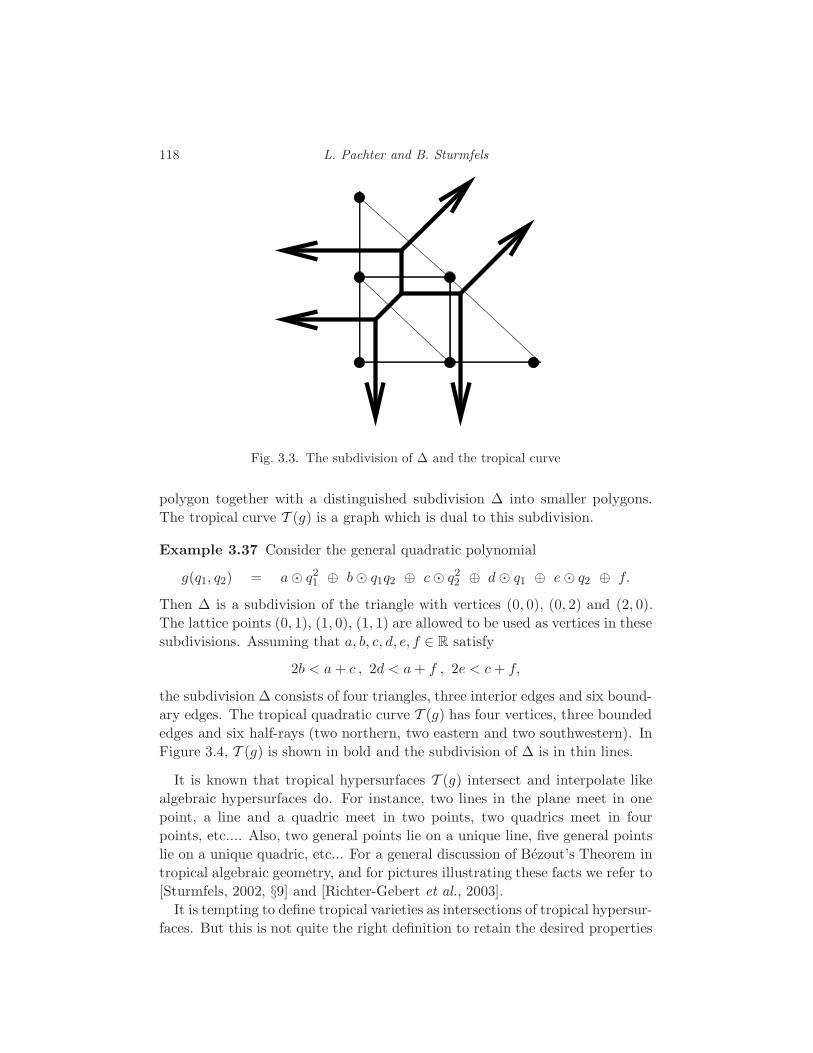
118 L. Pachter and B. Sturmfels
Fig. 3.3. The subdivision of ∆ and the tropical curve
polygon together with a distinguished subdivision ∆ into smaller polygons.
The tropical curve T (g) is a graph which is dual to this subdivision.
Example 3.37 Consider the general quadratic polynomial
g(q1, q2) = a⊙ q21 ⊕ b⊙ q1q2 ⊕ c⊙ q22 ⊕ d⊙ q1 ⊕ e⊙ q2 ⊕ f.
Then ∆ is a subdivision of the triangle with vertices (0, 0), (0, 2) and (2, 0).
The lattice points (0, 1), (1, 0), (1, 1) are allowed to be used as vertices in these
subdivisions. Assuming that a, b, c, d, e, f ∈ R satisfy
2b < a+ c , 2d < a+ f , 2e < c+ f,
the subdivision ∆ consists of four triangles, three interior edges and six bound-
ary edges. The tropical quadratic curve T (g) has four vertices, three bounded
edges and six half-rays (two northern, two eastern and two southwestern). In
Figure 3.4, T (g) is shown in bold and the subdivision of ∆ is in thin lines.
It is known that tropical hypersurfaces T (g) intersect and interpolate like
algebraic hypersurfaces do. For instance, two lines in the plane meet in one
point, a line and a quadric meet in two points, two quadrics meet in four
points, etc.... Also, two general points lie on a unique line, five general points
lie on a unique quadric, etc... For a general discussion of Bezout’s Theorem in
tropical algebraic geometry, and for pictures illustrating these facts we refer to
[Sturmfels, 2002, §9] and [Richter-Gebert et al., 2003].
It is tempting to define tropical varieties as intersections of tropical hypersur-
faces. But this is not quite the right definition to retain the desired properties
Algebra 119
from classical algebraic geometry. What we do instead is to utilize the field
Q(ǫ) of rational functions in one variable ǫ. We think of ǫ as a positive in-
finitesimal. Any non-zero rational function c(ǫ) ∈ Q(ǫ) has a series expansion
c(ǫ) = α0ǫi0 +α1ǫ
i1α2ǫi2 + · · · (where i0, i1, . . . ∈ Z, α0, α1, . . . ∈ Q , α0 6= 0)
This series is unique. The order of the rational function c(ǫ) is the integer i0.
Example 3.38 The following rational function in Q(ǫ) has order(c(ǫ)) = −2:
c(ǫ) =3ǫ4 + 8ǫ5 + ǫ7 − ǫ10
17ǫ6 − 11ǫ9 + 2ǫ13=
3
17ǫ−2 +
8
17ǫ−1 +
50
289ǫ1 +
88
289ǫ2 + · · ·
Let Q(ǫ)[p1, . . . , pm] be the ring of polynomials in m unknowns with coeffi-
cients in Q(ǫ). For any (classical) polynomial
f =
s∑
i=1
ci(ǫ) · pa1i1 pa2i
2 · · ·pamim ∈ Q(ǫ)[p1, . . . , pm], (3.33)
we define the tropicalization g = trop(f) to be the tropical polynomial
g =
s⊕
i=1
order(ci(ǫ))⊙ qa1i1 ⊙ qa2i
2 ⊙ · · · ⊙ qamim . (3.34)
In this manner, every polynomial f defines a tropical hypersurface T (g) =
T(trop(f)
)in Rm. Recall that the function g : Rm → R is given as the
minimum of s linear functions. The hypersurface T (g) consists of all points
q = (q1, . . . , qm) ∈ Rm where this minimum is attained at least twice, i.e.,
order(ci(ǫ)) + a1iq1 + · · ·+ amiqm = order(cj(ǫ)) + a1jq1 + · · ·+ amjqm
≤ order(ck(ǫ)) + a1kq1 + · · ·+ amkqm for i 6= j and k ∈ 1, . . . , s\i, j.
If, in addition to this condition, the leading coefficients α0 of the series ci(ǫ)
and cj(ǫ) are rational numbers of opposite signs then we say that q is a
positive point of T (g). The subset of all positive points in T (g) is denoted
T+(g) and called the positive tropical hypersurface of the polynomial f .
If the polynomial f in (3.33) does not depend on ǫ at all, i.e., if f ∈Q[p1, . . . , pm], then order(ci(ǫ)) = 0 for all coefficients of its tropicalization
g in (3.34), and the function g : Rm → R is given as the minimum of s linear
functions with zero constant terms. Here is an example where this is the case.
Example 3.39 Let m = 9 and consider the determinant of a 3 × 3-matrix
f = p11p22p33 − p11p23p32 − p12p21p33 + p12p23p31 + p13p21p32 − p13p22p31.
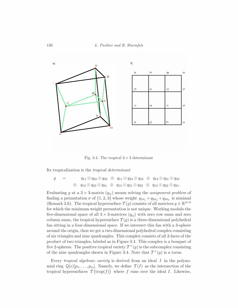
120 L. Pachter and B. Sturmfels
3 33 2
2 2 2 31 23 12 3 1 11 1
1 1 1 32 2 2 13 3 3 21 13 2 2 1 3 11 22 33 31 1 2 2
1 3
a ) b )
Fig. 3.4. The tropical 3 × 3 determinant
Its tropicalization is the tropical determinant
g = q11 ⊙ q22 ⊙ q33 ⊕ q11 ⊙ q23 ⊙ q32 ⊕ q12 ⊙ q21 ⊙ q33
⊕ q12 ⊙ q23 ⊙ q31 ⊕ q13 ⊙ q21 ⊙ q32 ⊕ q13 ⊙ q22 ⊙ q31.
Evaluating g at a 3 × 3-matrix (qij) means solving the assignment problem of
finding a permutation σ of 1, 2, 3 whose weight q1σ1 + q2σ2 + q3σ3 is minimal
(Remark 2.6). The tropical hypersurface T (g) consists of all matrices q ∈ R3×3
for which the minimum weight permutation is not unique. Working modulo the
five-dimensional space of all 3 × 3-matrices (qij) with zero row sums and zero
column sums, the tropical hypersurface T (g) is a three-dimensional polyhedral
fan sitting in a four-dimensional space. If we intersect this fan with a 3-sphere
around the origin, then we get a two-dimensional polyhedral complex consisting
of six triangles and nine quadrangles. This complex consists of all 2-faces of the
product of two triangles, labeled as in Figure 3.4. This complex is a bouquet of
five 2-spheres. The positive tropical variety T +(g) is the subcomplex consisting
of the nine quadrangles shown in Figure 3.4. Note that T +(g) is a torus.
Every tropical algebraic variety is derived from an ideal I in the polyno-
mial ring Q(ǫ)[p1, . . . , pm]. Namely, we define T (I) as the intersection of the
tropical hypersurfaces T(trop(f)
)where f runs over the ideal I . Likewise,
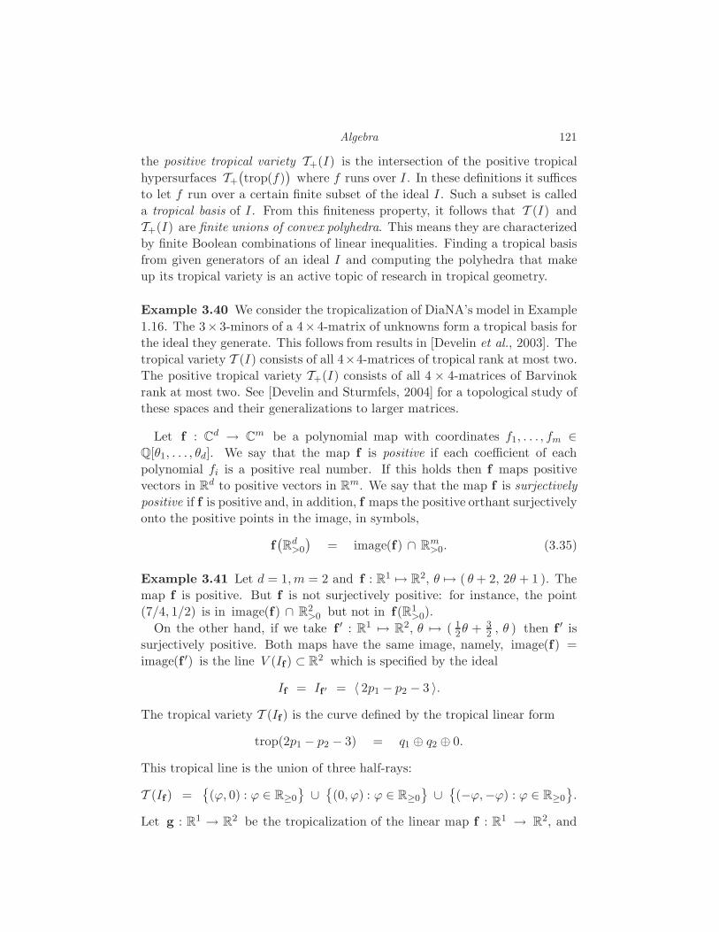
Algebra 121
the positive tropical variety T+(I) is the intersection of the positive tropical
hypersurfaces T+
(trop(f)
)where f runs over I . In these definitions it suffices
to let f run over a certain finite subset of the ideal I . Such a subset is called
a tropical basis of I . From this finiteness property, it follows that T (I) and
T+(I) are finite unions of convex polyhedra. This means they are characterized
by finite Boolean combinations of linear inequalities. Finding a tropical basis
from given generators of an ideal I and computing the polyhedra that make
up its tropical variety is an active topic of research in tropical geometry.
Example 3.40 We consider the tropicalization of DiaNA’s model in Example
1.16. The 3× 3-minors of a 4× 4-matrix of unknowns form a tropical basis for
the ideal they generate. This follows from results in [Develin et al., 2003]. The
tropical variety T (I) consists of all 4×4-matrices of tropical rank at most two.
The positive tropical variety T+(I) consists of all 4 × 4-matrices of Barvinok
rank at most two. See [Develin and Sturmfels, 2004] for a topological study of
these spaces and their generalizations to larger matrices.
Let f : Cd → Cm be a polynomial map with coordinates f1, . . . , fm ∈Q[θ1, . . . , θd]. We say that the map f is positive if each coefficient of each
polynomial fi is a positive real number. If this holds then f maps positive
vectors in Rd to positive vectors in Rm. We say that the map f is surjectively
positive if f is positive and, in addition, f maps the positive orthant surjectively
onto the positive points in the image, in symbols,
f(Rd
>0
)= image(f) ∩ Rm
>0. (3.35)
Example 3.41 Let d = 1, m = 2 and f : R1 7→ R2, θ 7→ ( θ+ 2, 2θ + 1 ). The
map f is positive. But f is not surjectively positive: for instance, the point
(7/4, 1/2) is in image(f) ∩ R2>0 but not in f(R1
>0).
On the other hand, if we take f ′ : R1 7→ R2, θ 7→ ( 12θ + 3
2 , θ ) then f ′ is
surjectively positive. Both maps have the same image, namely, image(f) =
image(f ′) is the line V (If ) ⊂ R2 which is specified by the ideal
If = If ′ = 〈 2p1 − p2 − 3 〉.
The tropical variety T (If ) is the curve defined by the tropical linear form
trop(2p1 − p2 − 3) = q1 ⊕ q2 ⊕ 0.
This tropical line is the union of three half-rays:
T (If ) =(ϕ, 0) : ϕ ∈ R≥0
∪(0, ϕ) : ϕ ∈ R≥0
∪(−ϕ,−ϕ) : ϕ ∈ R≥0
.
Let g : R1 → R2 be the tropicalization of the linear map f : R1 → R2, and
122 L. Pachter and B. Sturmfels
let g′ be the tropicalization of f ′. These piecewise-linear maps are given by
g(w) =(trop(f1)(w), trop(f2)(w)
)= (w ⊕ 0, w⊕ 0) = (min(w, 0),min(w, 0))
and g′(w) =(trop(f ′1)(w), trop(f ′2)(w)
)=(w ⊕ 0, w
)=(min(w, 0), w
).
These map R1 onto one or two of the three halfrays of the tropical line T (If ):
image(g) =(−ϕ,−ϕ) : ϕ ∈ R≥0
,
image(g′) =(0, ϕ) : ϕ ∈ R≥0
∪(−ϕ,−ϕ) : ϕ ∈ R≥0
= T+(If ).
The tropicalization g′ of the surjectively positive map f ′ maps onto the positive
tropical variety. This is an example for the result in Theorem 3.42 below.
Returning to our general discussion, consider an arbitrary polynomial map
f : Cd → Cm. The tropicalization of f is the piecewise-linear map
g : Rd → Rm , ϕ 7→(g1(ϕ), g2(ϕ), . . . , gm(ϕ)
), (3.36)
where gi = trop(fi) is the tropicalization of the ith coordinate polynomial fi
of f . To describe the geometry of the tropical polynomial map g, we consider
the Newton polytopes NP(f1),NP(f2), . . . ,NP(fm) of the coordinates of f .
Recall from Section 2.3 that the Newton polytope NP(fi) of the polynomial
fi is the convex hull of the vectors (u1, u2, . . . , ud) such that θu11 θu2
2 · · ·θudd
appears with non-zero coefficient in fi. The cones in the normal fan of the
Newton polytope NP(fi) are the domains of linearity of the piecewise-linear
map gi : Rd → Rm. The Newton polytope of the map f is defined as the
Newton polytope of the product of the coordinate polynomials:
NP(f) := NP(f1 · f2 · · · · · fm) = NP(f1)⊙NP(f2)⊙· · ·⊙NP(fm). (3.37)
The operation ⊙ on the right is the Minkowski sum of polytopes (Theorem
2.25). The following theorem describes the geometry of tropicalizing polyno-
mial maps.
Theorem 3.42 The tropical polynomial map g : Rd → Rm is linear on each
cone in the normal fan of the Newton polytope NP(f). Its image lies inside
the tropical variety T (If ). If f is positive then image(g) lies in the positive
tropical variety T+(If ). If f is surjectively positive then image(g) = T+(If ).
Proof See [Pachter and Sturmfels, 2004c] and [Speyer and Williams, 2004].
This theorem is fundamental for the study of inference functions of statis-
tical models in Chapter 9. Imagine that w ∈ Rd is a vector of weights for a
dynamic programming problem which is derived from a statistical model. The

Algebra 123
relationship between the weights and the model parameters is wi ∼ log(θi).
Evaluating the tropical map g at w means solving the dynamic programs for
all possible observations. As we vary the weights w, the vector of outcomes is
piecewise constant. Whenever w crosses a boundary, the system undergoes a
“phase transition”, meaning that the outcome changes for some observation.
Theorem 3.42 offers a geometric characterization of these phase transitions,
taking into account all possible weights and all possible observations.
If the model has only one parameter, then the Newton polytope NP(f) is a
line segment. There are only two “phases”, corresponding to the two vertices
of that segment. In Example 3.41 the “phase transition” occurs at w = 0.
One important application of this circle of ideas is sequence alignment (Sec-
tion 2.2). The statistical model for alignment is the pair HMM f in (2.15).
The tropicalization g of the polynomial map f is the tropicalized pair HMM,
whose coordinates gi are featured in (2.16). Parametric alignment is discussed
in Chapters 5, 7, 8 and 9. We conclude this section with two other examples.
Example 3.43 DiaNA’s model in Example 3.40 has d = 16 parameters
θ =(β1
A, β1C , β
1G, β
1T , β
2A, β
2C, β
2G, β
2T , γ
1A, γ
1C, γ
1G, γ
1T , γ
2A, γ
2C , γ
2G, γ
2T
),
and it is specified by the homogeneous polynomial map f : C16 7→ C4×4 with
pij = β1i β
2j + γ1
i γ2j , where i, j ∈ A, C, G, T.
We know from the linear algebra literature [Cohen and Rothblum, 1993] that
every positive 4×4-matrix of rank ≤ 2 is the sum of two positive 4×4-matrices
of rank ≤ 1. This means that DiaNA’s model f is a surjectively positive map.
The tropicalization of f is the piecewise-linear map g : R16 7→ R4×4 given by
qij = β1i ⊙ β2
j ⊕ γ1i ⊙ γ2
j = min(β1
i + β2j , γ
1i + γ2
j
)for i, j ∈ A, C, G, T.
Theorem 3.42 says that the image of g equals the positive tropical variety
T+(Ig). The space T+(Ig) consists of all 4 × 4-matrices of Barvinok rank ≤ 2
and was studied in [Develin et al., 2003] and [Develin and Sturmfels, 2004].
The Newton polytope NP(f) of the map f is a zonotope, i.e., it is a Minkowski
sum of line segments. The map g is piecewise linear with respect to the hyper-
plane arrangement dual to that zonotope. For a detailed combinatorial study
of the map g and the associated hyperplane arrangement see [Ardila, 2004].
Example 3.44 We consider the hidden Markov model of length n = 3 with
binary states (l = l′ = 2) but, in contrast to Example 3.19, we suppose that all
eight parameters θ00, θ01, θ10, θ11, θ′00, θ
′01, θ
′10, θ
′11 are independent unknowns.

124 L. Pachter and B. Sturmfels
Thus our model is the homogeneous map f : C8 → C8 with coordinates
fσ1σ2σ3 = θ00θ00θ′0σ1θ′0σ2
θ′0σ3+ θ00θ01θ
′0σ1θ′0σ2
θ′1σ3+ θ01θ10θ
′0σ1θ′1σ2
θ′0σ3
+θ01θ11θ′0σ1θ′1σ2
θ′1σ3+ θ10θ00θ
′1σ1θ′0σ2
θ′0σ3+ θ10θ01θ
′1σ1θ′0σ2
θ′1σ3
+ θ11θ10θ′1σ1θ′1σ2
θ′0σ3+ θ11θ11θ
′1σ1θ′1σ2
θ′1σ3.
The implicitization techniques of Section 3.2 reveal that If is generated by
p2011p
2100 − p2
001p2110 + p000p011p
2101 − p000p
2101p110 + p000p011p
2110
−p001p2010p111 + p2
001p100p111 + p2010p100p111 − p001p
2100p111 − p000p
2011p110
−p001p011p100p101 − p010p011p100p101 + p001p010p011p110 − p010p011p100p110
+p001p010p101p110 + p001p100p101p110 + p000p010p011p111 − p000p011p100p111
−p000p001p101p111 + p000p100p101p111 + p000p001p110p111 − p000p010p110p111.
Thus T (If ) is the tropical hypersurface defined by this degree four polynomial.
The tropicalized HMM is the map g : R8 → R8, (w, w′) 7→ q with coordinates
qσ1σ2σ3 = minwh1h2+wh2h3+w
′h1σ1
+w′h2σ2+w′h3σ3
: (h1, h2, h3) ∈ 0, 13.
This minimum is attained by the most likely explanation (h1, h2, h3) of the
observation (σ1, σ2, σ3). Inference means evaluating the tropical polynomials
qσ1σ2σ3 . For instance, for the parameters w =( 6 5
8 1
)and w′ =
(0 88 8
)we find:
The observation σ1σ2σ3 = 000 001 010 011 100 101 110 111
has the explanation h1h2h3 = 000 001 000 011 000 111 110 111
We call 0, 13 → 0, 13, σ1σ2σ3 7→ h1h2h3 the inference function for the
parameters (w, w′). There are 88 = 16, 777, 216 functions from 0, 13 to itself,
but only 398 of them are inference functions. In Chapter 9 it is shown that the
number of inference functions is polynomial in the sequence length n, while
the number of functions from 0, 1n to itself is doubly-exponential in n.
The inference functions are indexed by the vertices of the Newton polytope
NP(f). In our example, polymake reveals that NP(f) is 5-dimensional and has
398 vertices, 1136 edges, 1150 two-faces, 478 ridges and 68 facets. Thus there
are 398 inference functions, and we understand their phase transitions.
However, there are still many questions we do not yet know how to answer,
even for small n. What is the most practical method for listing all maximal
cones in the image of g ? How does the number of these cones compare to
the number of vertices of NP(f)? Is the hidden Markov model f surjectively
positive? Which points of the positive tropical variety T+(If ) lie in image(g)?
Algebra 125
3.5 The tree of life and other tropical varieties
At the 1998 International Congress of Mathematicians in Zurich, Andreas
Dress presented an invited lecture titled “The tree of life and other affine build-
ings” [Dress and Terhalle, 1998]. Our section title is meant as a reference to
that paper, which highlighted the importance and utility of understanding the
geometry and structure of phylogenetic trees and networks. In Chapter 4, we
return to this topic by explaining how the space of trees and its generalizations
is relevant for modeling and reconstructing the tree of life.
Here we begin with a reminder of the definition of metrics and tree metrics,
which were introduced in Section 2.4. A metric on [n] = 1, 2, . . . , n is a
dissimilarity map for which the triangle inequality holds. Of course, most
metrics D are not tree metrics. The set of tree metrics is the space of trees Tn.
This is a (2n − 3)-dimensional polyhedral fan inside(n2
)-dimensional cone of
all metrics. Membership in Tn is characterized by the Four Point Condition.
Our goal here is to derive an interpretation of Tn in tropical geometry.
Let Q = (qij) be a symmetric matrix with zeros on the diagonal whose(n2
)distinct off-diagonal entries are unknowns. For each quadruple i, j, k, l
⊂ 1, 2, . . . , n we consider the quadratic tropical polynomial
gijkl(Q) = qij ⊙ qkl ⊕ qik ⊙ qjl ⊕ qil ⊙ qjk. (3.38)
This tropical polynomial is the tropicalization of the Plucker relation (3.14)
gijkl(Q) = trop(pikpjl − pijpkl − pilpjk)
which defines a tropical hypersurface T (gijkl) in the space R(n2). In fact,
the Plucker relations (3.14) form a tropical basis for the Plucker ideal I2,n
[Speyer and Sturmfels, 2004]. This implies that the tropical Grassmannian
T (I2,n) equals the intersection of these(n4
)tropical hypersurfaces, i.e.,
T (I2,n) =⋂
1≤i<j<k<l≤n
T (gijkl) ⊂ R(n2). (3.39)
Theorem 3.45 The space of trees Tn is (up to sign) the tropical Grassman-
nian T (I2,n).
Proof A metric D = (dij) is a point in the space of trees Tn if and only if
the four point condition holds. This condition states that, for all 1 ≤ i < j <
k < l ≤ n, the maximum of dij + dkl, dik + djl, dil + djk is attained at least
twice. If Q = (qij) = −D = (−dij) then this is equivalent to saying that the
minimum of qij + qkl, qik + qjl, qil + qjk is attained at least twice. This is
precisely the condition for Q to be in the tropical hypersurface T (gijkl).

126 L. Pachter and B. Sturmfels
Example 3.46 The space of trees on five taxa [5] = 1, 2, 3, 4, 5 is (up to
sign) a tropical variety of codimension three in R10. It is not the intersection
of three tropical hypersurfaces, but it is the intersection of five hypersurfaces:
T (I2,5) = −T5 = T (q12 ⊙ q34 ⊕ q13 ⊙ q24 ⊕ q14 ⊙ q23)
∩ T (q12 ⊙ q35 ⊕ q13 ⊙ q25 ⊕ q15 ⊙ q23)
∩ T (q12 ⊙ q45 ⊕ q14 ⊙ q25 ⊕ q15 ⊙ q24)
∩ T (q13 ⊙ q45 ⊕ q14 ⊙ q35 ⊕ q15 ⊙ q34)
∩ T (q23 ⊙ q45 ⊕ q24 ⊙ q35 ⊕ q25 ⊙ q34).
The space of trees T5 is the union of 15 seven-dimensional cones in R10≥0. Each
cone is the solution set to a system of linear inequalities such as
q12 + q34 ≥ q13 + q24 = q14 + q23,
q12 + q35 ≥ q13 + q25 = q15 + q23,
q12 + q45 ≥ q14 + q25 = q15 + q24,
q13 + q45 ≥ q14 + q35 = q15 + q34,
and q23 + q45 ≥ q24 + q35 = q25 + q34.
The seven-dimensional cone specified by this linear system is isomorphic to
R7≥0, and corresponds to the tree with splits (12, 345) and (123, 45).
The combinatorial structure of the space T5 is that of the Petersen graph,
shown in Figure 3.5. Vertices of the Petersen graph correspond to trees with
polytomy, i.e trees with internal vertices of degree at least 4. The edges corre-
spond to the seven-dimensional cones in T5. Two cones share a six-dimensional
facet if and only if the two edges share a node in the Petersen graph.
The interpretation of the space of trees as a tropical Grassmannian opens
up the possibility of modeling a wide range of problems in phylogenetics us-
ing tropical geometry. We shall demonstrate this by tropicalizing the higher
Grassmannian Gd,n = V (Id,n) and the Pfaffian varieties V (I2,n,k) which we
encountered towards the end of Section 3.2. We begin with a discussion of
tropical linear spaces. These are relevant for evolutionary biology because:
• Trees are tropical lines.
• Higher-dimensional trees are tropical linear spaces.
The second statement will be made precise in Theorem 3.47.
A tropical hyperplane in Rn is any subset of Rn which has the form T (ℓ),
where ℓ is a tropical linear form in n unknowns qi:
ℓ(q) = a1 ⊙ q1 ⊕ a2 ⊙ q2 ⊕ · · · ⊕ an ⊙ qn.
Here a1, . . . an are arbitrary constants in R∪∞. Solving linear equations
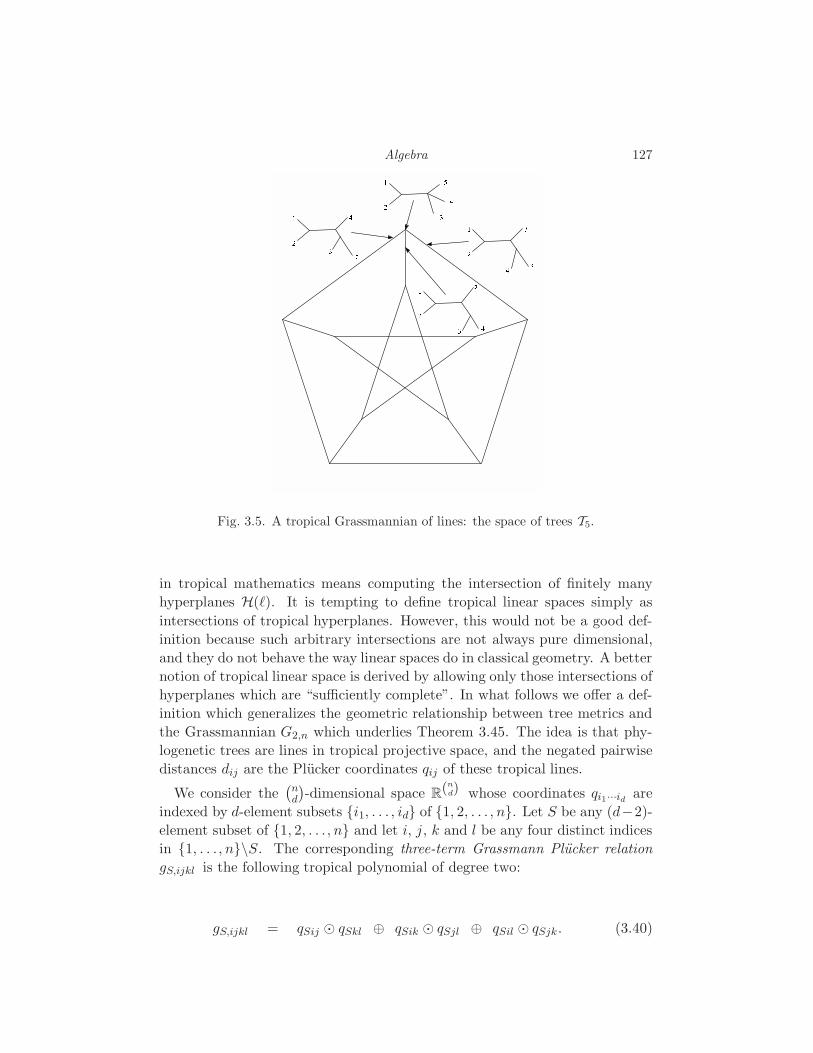
Algebra 127
12 34 512 43 5 12 53 412 53 4
Fig. 3.5. A tropical Grassmannian of lines: the space of trees T5.
in tropical mathematics means computing the intersection of finitely many
hyperplanes H(ℓ). It is tempting to define tropical linear spaces simply as
intersections of tropical hyperplanes. However, this would not be a good def-
inition because such arbitrary intersections are not always pure dimensional,
and they do not behave the way linear spaces do in classical geometry. A better
notion of tropical linear space is derived by allowing only those intersections of
hyperplanes which are “sufficiently complete”. In what follows we offer a def-
inition which generalizes the geometric relationship between tree metrics and
the Grassmannian G2,n which underlies Theorem 3.45. The idea is that phy-
logenetic trees are lines in tropical projective space, and the negated pairwise
distances dij are the Plucker coordinates qij of these tropical lines.
We consider the(nd
)-dimensional space R(n
d) whose coordinates qi1···id are
indexed by d-element subsets i1, . . . , id of 1, 2, . . . , n. Let S be any (d−2)-
element subset of 1, 2, . . . , n and let i, j, k and l be any four distinct indices
in 1, . . . , n\S. The corresponding three-term Grassmann Plucker relation
gS,ijkl is the following tropical polynomial of degree two:
gS,ijkl = qSij ⊙ qSkl ⊕ qSik ⊙ qSjl ⊕ qSil ⊙ qSjk. (3.40)

128 L. Pachter and B. Sturmfels
We define the space of d-trees to be the intersection of these hypersurfaces,
Td,n :=⋂
S,i,j,k,l
T (gS,ijkl) ⊂ R(nd), (3.41)
where the intersection is over all S, i, j, k, l as above. If d = 2 then S = ∅, the
polynomial (3.40) is the four point condition (3.38), and T2,n is the space of
trees Tn = T (I2,n). For d ≥ 3, the tropical Grassmannian T (Id,n) is contained
in the space of d-trees Td,n, and this containment is proper for n ≥ d + 4.
However, Td,n is a good combinatorial approximation for T (Id,n).
The points Q = (qi1···id) in Td,n ⊂ R(nd) are called d-trees. Fix a d-tree Q.
For any (d+1)-subset j0, j1, . . . , jd of 1, 2, . . . , nwe consider the hyperplane
specified by the following tropical linear form in the unknowns x1, . . . , xn:
ℓQj0j1···jd=
d⊕
r=0
qj0···bjr ···jd⊙ xr. (3.42)
The tropical linear space associated with the d-tree Q is the intersection
LQ =⋂
T (ℓQj0j1···jn) ⊂ Rn. (3.43)
Here the intersection is over all (d+ 1)-subsets j0, j1, . . . , jd of 1, 2, . . . , n.The “sufficient completeness” referred to above means that we need to solve
linear equations using Cramer’s rule, in all possible ways, in order for the
intersection of hyperplanes to be a linear space. The definition of linear space
given here is more inclusive than the notion one would get by tropicalizing
linear spaces over the field Q(ǫ). The latter are the tropical linear spaces LQ
where Q is any point in the subset T (Id,n) of TGd,n. [Speyer, 2004] proved
that all tropical linear spaces LQ are pure-dimensional polyhedral fans.
Theorem 3.47 (Speyer’s Theorem) Let Q ∈ Td,n be a d-tree. Then every
maximal cone of the tropical linear space LQ is d-dimensional.
Tropical linear spaces have many of the properties of ordinary linear spaces.
First, they have the correct dimension d. Second, every tropical linear space
LQ determines its vector of tropical Plucker coordinates Q uniquely up to
tropical multiplication (= classical addition) by a common scalar. If L and
L′ are tropical linear spaces of dimensions d and d′ with d + d′ ≥ n, then L
and L′ meet. It is not quite true that two tropical linear spaces intersect in a
tropical linear space but it is almost true. If L and L′ are tropical linear spaces
of dimensions d and d′ with d+ d′ ≥ n and v ∈ Rn is generic then L∩ (L′+ v)
is a tropical linear space of dimension d+ d′ − n. One then defines the stable
intersection of L and L′ by taking the limit of L ∩ (L′ + v) as v goes to zero.
Not every d-dimensional tropical linear space in Rn is the intersection of
Algebra 129
n − d tropical hyperplanes. It is an open problem to determine the minimum
number of tropical hyperplanes needed to cut out any tropical linear space of
dimension d in Rn. From (3.43) we see that( nd+1
)hyperplanes suffice.
Theorem 3.47 is relevant for phylogenetics because tropical linear spaces can
be regarded as “higher-dimensional phylogenetic trees”. Indeed, suppose we
have n taxa and we are given a dissimilarity measurement −qi1i2···id for any d-
tuple i1, i2, . . . , id of taxa in [n]. These(nd
)real numbers form a d-dimensional
dissimilarity matrix Q = (qi1i2···id) ∈ R(nd). Such a dissimilarity matrix Q is
the input for the Generalized Neighbor Joining Algorithm in Section 2.4
The tropical linear space LQ is a geometric model which plays the role of
the tree for the data Q. Indeed, passing from Rn to the (n − 1)-dimensional
tropical projective space Rn/R(1, 1, . . . , 1), the tropical linear space LQ is a
contractible polyhedral complex of pure dimension d − 1. In the classical
case d = 2, the linear space LQ is a pure-dimensional contractible polyhedral
complex of dimension 1, namely, it is precisely the tree with tree metric −Q.
Example 3.48 Fix d = 3 and n = 6. The dissimilarity of any triple i, j, kof taxa in [6] = 1, 2, 3, 4, 5, 6 is denoted by dijk, and we set qijk = −dijk. A
point Q = (qijk) ∈ R20 is a 3-tree if and only if the map (i, j) 7→ dijk is a tree
metric on [6]\k for all k ∈ [6]. Suppose this holds. Then the intersection
of the(64
)= 15 tropical hyperplanes T (ℓQj0j1j2j3
), is a 3-dimensional tropical
linear subspace LQ ⊂ R6. Each of the 15 defining linear forms has four terms:
ℓQj0j1j2j3
= qj0j1j2 ⊙ xj3 ⊕ qj0j1j3 ⊙ xj2 ⊕ qj0j2j3 ⊙ xj1 ⊕ qj1j2j3 ⊙ xj0 .
If we work in tropical projective 5-space, i.e. modulo the equivalence relation
(x1, x2, x3, x4, x5, x6) ≡ λ⊙ (x1, x2, x3, x4, x5, x6),
then LQ is a union of planar polygons. We call LQ a phylogenetic surface.
A phylogenetic surface is a two-dimensional geometric representation of the
dissimilarities among triples of taxa, just like a phylogenetic tree is a two-
dimensional geometric representation of the dissimilarities among pairs of taxa.
Embedded in the unbounded part of the phylogenetic surface LQ, we find the
six phylogenetic trees representing the tree metrics (i, j) 7→ dijk for fixed k.
There are 1035 combinatorial types of phylogenetic surfaces on six taxa
[Speyer and Sturmfels, 2004]. They correspond to the maximal cones of the
tropical Grassmannian T (I3,6) = T3,6, just like the 15 binary trees on five
taxa correspond to the edges of the Petersen graph T2,5. If we replace R20
by its quotient modulo the subspace of dissimilarity maps of the particular
form dijk = ωi +ωj +ωk, then T3,6 is a three-dimensional simplicial complex
consisting of 65 vertices, 550 edges, 1395 triangles and 1035 tetrahedra. For the
topologically inclined, we note that the space T3,6 of phylogenetic surfaces (i.e.,

130 L. Pachter and B. Sturmfels
the space of 3-trees on 6 taxa) is a bouquet of 126 three-dimensional spheres,
just like the Petersen graph is a bouquet of 6 one-dimensional spheres.
We next discuss the tropical variety of the Pfaffian ideal I2,n,k and we offer a
phylogenetic interpretation which generalizes the space of tree Tn (the special
case k = 2). Suppose that D(1), . . . , D(r) are n × n-matrices which represent
metrics. We define a new metric, denoted D(1) ∨ · · · ∨ D(r) and called the
mixture of the given metrics, by taking the maximum distance for each pair:
(D(1) ∨ · · · ∨D(r))ij := max(D(1)ij , . . . , D
(r)ij ).
Equivalently, using tropical matrix addition, the mixture of the r metrics is
D(1) ∨ · · · ∨D(r) := −((−D(1)) ⊕ · · · ⊕ (−D(r))
)(3.44)
The term “mixture” conveys the idea that each metric D(ν) corresponds to
a random variable X (ν) on the pairs of taxa with probability distribution
Prob(X (ν) = i, j) ∼ exp(−τD(ν)ij ).
Consider a mixture of these r random variables where τ ≫ 0 and the mixing
probabilities p1, . . . , pr are positive. Then the mixed distribution satisfies
Prob(X (ν) = i, j) ∼r∑
ν=1
pν · exp(−τD(ν)ij ) ∼ exp
(−τ(D(1) ⊕ · · ·⊕D(r))ij
),
Thus defining the mixture of metrics as their sum in max-plus-algebra is a
natural thing to do in the context of tropical geometry of statistical models.
We say that a metric D has tree rank ≤ r if there exist tree metrics D(1),
. . . , D(r) such that D = D(1) ∨ · · · ∨D(r). Let T rn denote the subset of R(n
2)
consisting of all metrics of tree rank ≤ r. This is a polyhedral fan, generalizing
the space of trees (the case r = 1 = k−1). We propose the following problem:
characterize membership in T rn and study the structure of this space.
This problem may be relevant for the following issue in comparative ge-
nomics. If we are given an alignment of genomes then different regions (e.g. dif-
ferent genes) may give rise to different trees. It is desirable to create some
consensus among the conflicting tree metrics. The resulting consensus object
may no longer be tree-like, for instance, if we apply the refined techniques of
Chapter 17. Mixtures of tree metrics may be useful models for such situations.
Fix a metric D and consider an even subset i1, . . . , i2m of 1, 2, . . . , n.This subset defines a complete graph K2m with edge weights dijik . A matching
is a 1-regular subgraph of K2m. The weight of a matching is the sum of the
weights of its m edges. We are interested in the condition on D that each
complete subgroup K2m has more than one matching of maximum weight.

Algebra 131
Proposition 3.49 If a metric D has tree rank ≤ r then for every subset of
2r + 2 taxa, the maximum matching among these taxa is not unique.
For r = 1 this is precisely the Four-Point Condition. In view of (3.16), we
can rephrase Proposition 3.49 by tropicalizing the Pfaffians of order 2r + 2.
For instance, for r = 2, tropicalizing (3.17) yields the tropical 6 × 6-Pfaffian
q14 ⊙ q25 ⊙ q36 ⊕ q15 ⊙ q24 ⊙ q36 ⊕ q14 ⊙ q26 ⊙ q35 ⊕ q15 ⊙ q26 ⊙ q34
⊕ q16 ⊙ q24 ⊙ q35 ⊕ q16 ⊙ q25 ⊙ q34 ⊕ q13 ⊙ q26 ⊙ q45 ⊕ q12 ⊙ q36 ⊙ q45
⊕ q16 ⊙ q23 ⊙ q45 ⊕ q13 ⊙ q25 ⊙ q46 ⊕ q12 ⊙ q35 ⊙ q46 ⊕ q15 ⊙ q23 ⊙ q46
⊕ q13 ⊙ q24 ⊙ q56 ⊕ q12 ⊙ q34 ⊙ q56 ⊕ q14 ⊙ q23 ⊙ q56.
Evaluating this tropical polynomial means finding the minimum weight match-
ing in the complete graph K6. We see that Proposition 3.49 is equivalent to
Proposition 3.50 If a metric D has tree rank ≤ r then −D lies in the inter-
section of the tropical hypersurfaces defined by the subpfaffians of order 2r+2.
Proof Theorem 3.45 implies that, for each i ∈ 1, 2, . . . , r, there exists a
skew-symmetric n × n-matrix P (i) over the field Q(ǫ) such that P (i) has rank
2 and order(P (i)) = −D(i). These matrices can be chosen so that there is no
cancellation of leading terms when forming the sum P := P (1) + · · · + P (r).
Then order(P ) = −D and rank(P ) ≤ 2r. Every Pfaffian of order 2r + 2
vanishes for P . Hence −D lies on these tropical Pfaffian hypersurfaces.
This proof shows how algebraic geometry in conjunction with tropicalization
can suggest combinatorial constructions which may be useful for phylogenetics.
We are not claiming that algebraic geometry is needed for the proof; indeed,
it is easy to prove Proposition 3.49 without algebra. That is not the point.
Unfortunately, our necessary condition for membership in T rn is not suffi-
cient. The following counterexample for n = 6, r = 2 is due to David Bryant.
Example 3.51 Consider the path metric of K6 with a cycle removed:
D =
0 2 1 1 1 2
2 0 2 1 1 1
1 2 0 2 1 1
1 1 2 0 2 1
1 1 1 2 0 2
2 1 1 1 2 0
The maximum matching is attained twice, that is, −D lies in the tropical
hypersurface of the 6 × 6-Pfaffian. By examining all possible cases, one sees

132 L. Pachter and B. Sturmfels
that D cannot be written as the mixture D(1) ∨D(2) of two tree metrics. The
tree rank of D is 3. Thus the converse to Proposition 3.50 does not hold.
At this point, it is natural to make the following conjecture: If every restric-
tion of a matrixD to six points is the mixture of two trees then D is a mixture
of two trees. Or, more generally: If every restriction of D to 2r+ 2 points is a
mixture of r trees then D is a mixture of r trees.

4
Biology
Lior Pachter
Bernd Sturmfels
The purpose of this chapter is to describe genome sequence data and to explain
the relevance of the statistics and algebra we have discussed in Chapters 1–3
to understanding the function of genomes and their evolution. It sets the stage
for the studies in biological sequence analysis in some of the later chapters.
Given that mathematics and statistics play an increasingly important role
in many different aspects of biology, the question arises: why the emphasis on
genome sequences? The most significant answer is that genomes are fundamen-
tal objects which carry instructions for the self-assembly of living organisms.
Ultimately, our understanding of human biology will be based on an under-
standing of the organization and function of our genome. Also relevant to the
study of genomes, is the fact that there are large quantities of high fidelity
data. Current finished genome sequences have less than one error in 10, 000
bases. Statistical methods can therefore be directly applied to modeling the
random evolution of genomes and to making inferences about the structure and
organization of functional elements; there is no need to worry about extract-
ing signal from noisy data. Furthermore, it is frequently possible to validate
findings with laboratory experiments.
The rate of accumulation of genome sequence data has been extraordinary,
far outpacing Moore’s law for the density of transistors on circuit chips. This
is due to breakthroughs in sequencing technologies and radical advances in
automation. Thus, since the first completion of the genome of a free living or-
ganism in 1995 (Haemophilus Influenza [Fleischmann et al., 1995]), there are
now over 200 completely sequenced microbial genomes, and numerous com-
plete invertebrate and vertebrate genomes. The highlight of the sequencing
projects, from our Homo sapiens perspective, has been the completion of se-
quencing of the human genome which was formally announced at the end of
2004 [Human Genome Sequencing Consortium, 2004]. Our discussion of on-
line resources in Section 4.2 explains how one reads the human genome.
133
134 L. Pachter and B. Sturmfels
4.1 Genomes
Every living organism has a genome, made up of deoxyribonucleic acids (DNA)
arranged in a double helix [Watson and Crick, 1953], which encodes (in a way
to be made precise) the fundamental ingredients of life. Organisms are di-
vided into two major classes: eukaryotes (organisms whose cells contain a
nucleus) and prokaryotes (for example bacteria and archaea). In this book
we focus on genomes of eukaryotes, and, in particular, on genomes of verte-
brates (see Chapters 21 and 22). The primary example is the human genome
[Human Genome Sequencing Consortium, 2004, Venter et al., 2001]. This al-
lows for the description of ongoing genome projects at the forefront of current
research interests, while limiting the scope so that some detail can be provided
on how to obtain and utilize the data.
Eukaryotic genomes are divided into chromosomes. Each cell has two copies
of each chromosome. There are 23 pairs of chromosomes: 22 autosomes (two
copies each in both men and women) and two sex chromosomes, which are de-
noted X and Y. Women have two X chromosomes, while men have one X and
one Y chromosome. Parents pass on a mosaic of their pairs of chromosomes
to their children. Theoretical aspects of genetic inheritance are studied in the
well-established field of statistical genetics. A connection between genetics and
algebraic statistics was recently explored in [Hallgrimsdottir and Sturmfels, 2004].
The sequence of DNA molecules in a genome is typically represented as a
sequence of letters, partitioned into chromosomes, from the four letter alphabet
Σ = A, C, G, T. These letters correspond to the bases in the double helix,
that is, the nucleotides Adenine, Cytosine, Guanine and Thymine. The four
nucleotides fall into two pairs: purines (A and G) and pyrimidines (C and T).
This grouping comes about because of the chemistry of the nucleotides: the
purines have two rings in their structure while pyrimidines have only one. In
addition to this grouping, every DNA base in the double helix is paired with a
complementary base on the opposite helix. A is paired with T, and C with G, with
hydrogen bonding serving as the main force holding the two separate chains
together. Figure 4.1 illustrates these structural features of the nucleotides.
Remark 4.1 There is a natural action by the group Z2 ×Z2 on the alphabet
Σ = A, C, G, T. This action arises by the grouping into purines and pyrim-
idines, and from the complementarity of the bases. Keeping in mind that
finite abelian groups are (non-canonically) isomorphic to their dual groups,
this leads to an identification of the nucleotides in Σ = A, C, G, T with the
group elements in Z2 ×Z2. This structure is the rationale behind group based
evolutionary models, which we discuss in Section 4.4 and Chapters 15–17.
One of the consequences of DNA complementarity is Chargaff’s rule, which

Biology 135
Fig. 4.1. The four DNA bases.
states that every DNA sample must contain the same number of A’s as T’s,
and the same number of G’s as C’s [Chargaff, 1950]. Thus, in order to describe
a genome, it suffices to list the bases in only one strand of the double helix.
However, it is important to note that the two strands have a directionality.
The two directions are indicated by the numbers 5′ and 3′ on the ends. These
numbers correspond to carbon atoms in the helix backbone. The convention
is to write a single strand of DNA bases in the 5′ → 3′ direction.
Example 4.2 The DNA sequence GATATAGAGCGGATTACAG of length 20 is
shorthand for the double stranded sequence consisting of twenty base pairs
5’ GATATCAGAGCGGATTACAG 3’
3’ CTATAGTCTCGCCTAATGTC 5’
which in turn is shorthand for the bases along the DNA double helix.
The human genome consists of approximately 2.8 billion base pairs, and
has been obtained using high throughput sequencing technologies which allow
for reading short fragments only hundreds of bases long. Sequence assembly
algorithms are then necessary for piecing together the fragments [Myers, 1999].
Despite the tendency to abstract genomes as strings over the alphabet Σ,
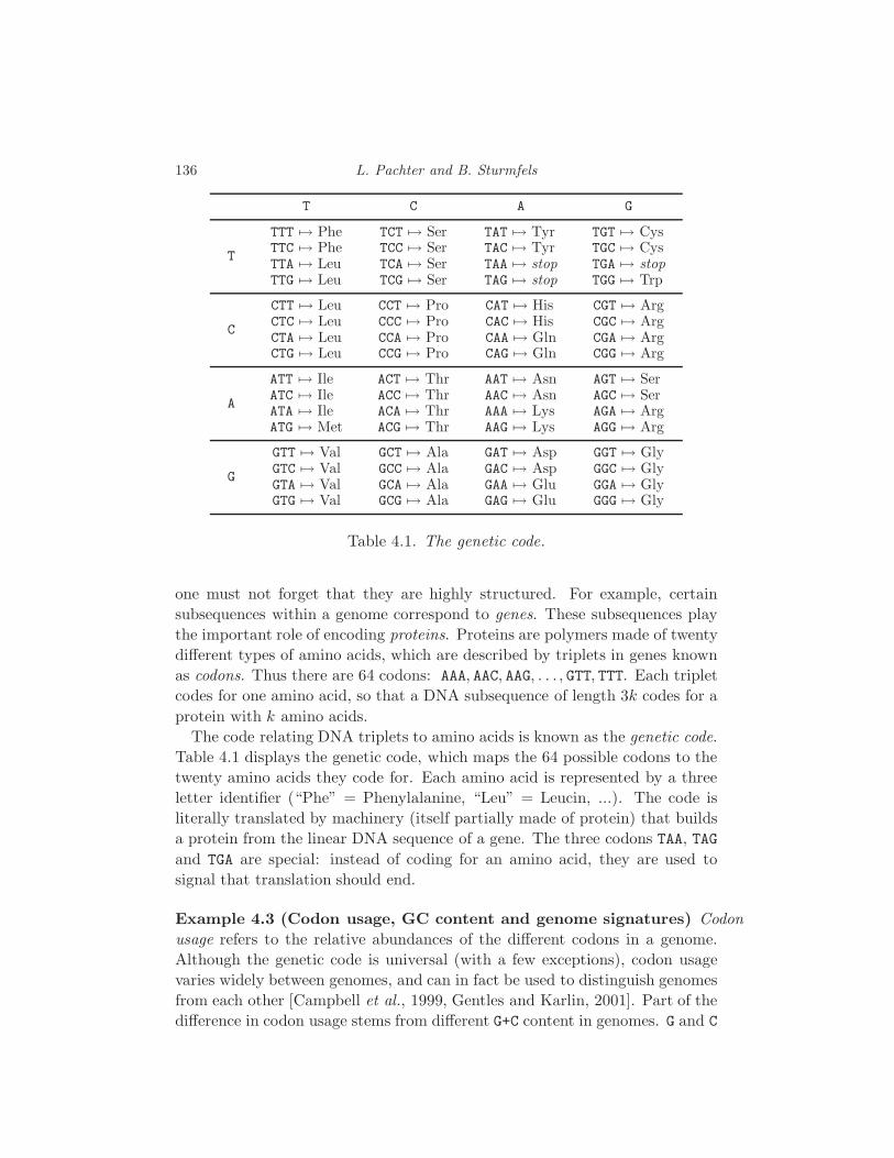
136 L. Pachter and B. Sturmfels
T C A G
T
TTT 7→ PheTTC 7→ PheTTA 7→ LeuTTG 7→ Leu
TCT 7→ SerTCC 7→ SerTCA 7→ SerTCG 7→ Ser
TAT 7→ TyrTAC 7→ TyrTAA 7→ stopTAG 7→ stop
TGT 7→ CysTGC 7→ CysTGA 7→ stopTGG 7→ Trp
C
CTT 7→ LeuCTC 7→ LeuCTA 7→ LeuCTG 7→ Leu
CCT 7→ ProCCC 7→ ProCCA 7→ ProCCG 7→ Pro
CAT 7→ HisCAC 7→ HisCAA 7→ GlnCAG 7→ Gln
CGT 7→ ArgCGC 7→ ArgCGA 7→ ArgCGG 7→ Arg
A
ATT 7→ IleATC 7→ IleATA 7→ IleATG 7→ Met
ACT 7→ ThrACC 7→ ThrACA 7→ ThrACG 7→ Thr
AAT 7→ AsnAAC 7→ AsnAAA 7→ LysAAG 7→ Lys
AGT 7→ SerAGC 7→ SerAGA 7→ ArgAGG 7→ Arg
G
GTT 7→ ValGTC 7→ ValGTA 7→ ValGTG 7→ Val
GCT 7→ AlaGCC 7→ AlaGCA 7→ AlaGCG 7→ Ala
GAT 7→ AspGAC 7→ AspGAA 7→ GluGAG 7→ Glu
GGT 7→ GlyGGC 7→ GlyGGA 7→ GlyGGG 7→ Gly
Table 4.1. The genetic code.
one must not forget that they are highly structured. For example, certain
subsequences within a genome correspond to genes. These subsequences play
the important role of encoding proteins. Proteins are polymers made of twenty
different types of amino acids, which are described by triplets in genes known
as codons. Thus there are 64 codons: AAA, AAC, AAG, . . . , GTT, TTT. Each triplet
codes for one amino acid, so that a DNA subsequence of length 3k codes for a
protein with k amino acids.
The code relating DNA triplets to amino acids is known as the genetic code.
Table 4.1 displays the genetic code, which maps the 64 possible codons to the
twenty amino acids they code for. Each amino acid is represented by a three
letter identifier (“Phe” = Phenylalanine, “Leu” = Leucin, ...). The code is
literally translated by machinery (itself partially made of protein) that builds
a protein from the linear DNA sequence of a gene. The three codons TAA, TAG
and TGA are special: instead of coding for an amino acid, they are used to
signal that translation should end.
Example 4.3 (Codon usage, GC content and genome signatures) Codon
usage refers to the relative abundances of the different codons in a genome.
Although the genetic code is universal (with a few exceptions), codon usage
varies widely between genomes, and can in fact be used to distinguish genomes
from each other [Campbell et al., 1999, Gentles and Karlin, 2001]. Part of the
difference in codon usage stems from different G+C content in genomes. G and C
Biology 137
nucleotides are known to be involved in a number of genome regulation mech-
anisms. For example, CpG sites are locations in DNA sequences where a C is
adjacent and upstream of a G. DNA methyltransferase recognizes CpG sites and
converts the cytosine into 5-methylcytosine. Spontaneous deamination causes
the 5-methylcytosine to be converted into thymine, and the mutation is not
fixed by DNA repair mechanisms. This results in a gradual erosion of CpG
sites in the genome. CpG islands are regions of DNA with many unmethylated
CpG sites. Spontaneous deamination of cytosine to thymine in these sites is
repaired, resulting in a restored CpG site. Such sites are associated with pro-
moter regions of genes. CpG islands alone, however, do not explain the vast
differences in G+C content seen between genomes.
A simple model for genome signatures that distinguish organisms is a din-
ucleotide model [Campbell et al., 1999]. Specifically, the data consists of 16
numbers uij, i, j ∈ A,C,G, T, where uij counts the number of times that
the pair of nucleotides ij appear consecutively in that order in a genome. The
independence model for dinucleotides is ...
In order to make protein, DNA is first copied into a similar molecule called
RNA (this process is called transcription). It is the RNA that is translated into
protein. The link between DNA, RNA and protein is the basis of molecular
biology, and is sometimes referred to as the central dogma.
When protein is created from DNA, the gene that has been translated is
said to have been expressed. Proteins can be structural elements, or perform
complex tasks (such as regulation of expression) by interacting with the many
molecules and complexes in cells. Thus, the genome is a blueprint for life. A
major goal in biology, to be discussed in Section 4.3, is a complete understand-
ing of the genes, the function of their proteins, and their expression patterns.
The human genome contains approximately 25,000 genes, although the exact
number has still not been determined [Human Genome Sequencing Consortium, 2004].
While there are experimental methods for discovering and validating genes,
there is still no high throughput technology for accurately identifying all the
genes in a genome. The computational problem of identifying genes, the gene
finding problem, is an active area of research [Dewey et al., 2004, Korf et al., 2001].
One of the main difficulties lies in the fact that only a small portion of the
genome is genic; in fact, less than 5% of the genome is known to be functional.
In Section 4.4 we discuss this problem, and the role of statistical models in
formulating sound methods for distinguishing genes from non-genic sequence.
The models of choice are the hidden Markov models whose mathematical char-
acterization was discussed in Section 1.4. Hidden Markov models allow for the
integration of diverse biological information (such as the genetic code and the
structure of genes) and are suitable for designing efficient algorithms. In spite

138 L. Pachter and B. Sturmfels
of much progress, the current understanding of genes is not sufficient to allow
for the ab-initio identification of all the genes in a genome [Guigo et al., 2004].
A key idea in biology has been that the comparison of multiple genome
sequences can assist in identifying genes and other functional elements. The
underlying premise of the comparative genomics approach is that although
DNA sequences change over time, functional elements such as genes will tend
to be conserved due to their critical role in coding for proteins or other impor-
tant elements. The comparative genomics approach therefore seeks to utilize
Darwin’s principle of natural selection to sift through genome sequences for
functional elements. The principle has been applied to collections of similar
genomes [Boffelli et al., 2003, Boffelli et al., 2004b], as well as more diverged
sequences [Gibbs et al., 2004, Hillier et al., 2004].
The different types of comparisons require an understanding of the underly-
ing biology. For example, differences between the genomes of individuals in a
population are small and are primarily due to recombination events (the pro-
cess by which two copies of parental chromosomes are merged in the offspring).
On the other hand, the genomes of different species (classes of organisms that
can produce offspring together) tend to be much more diverse. Genome dif-
ferences between species are a result of numerous transformations of genome
sequences:
• Genome rearrangement – comparing chromosomes of related species reveals
large segments that have been reversed and flipped (inversions), segments
that have been moved (transpositions), fusions of chromosomes, and other
large scale events. Methods of combinatorial mathematics have led to signifi-
cant progress in this field [Hannenhalli and Pevzner, 1999, Tesler, 2002], but
the underlying biological mechanisms are still poorly understood [Sankoff and Nadeau, 2003].
• Duplications and loss – some genomes have undergone whole genome duplica-
tions. This process was recently demonstrated for yeast [Kellis et al., 2004].
Individual chromosomes or genes may also be duplicated. Duplication events
are often accompanied by gene loss, as redundant genes slowly lose or adapt
their function over time [Eichler and Sankoff, 2003].
• Parasitic expansion – large sections of genomes are repetitive, consisting of
elements which can duplicate and re-integrate into a genome [Brown, 2002].
• Point mutation, insertion and deletion – DNA sequences mutate, and in
non-functional regions these mutations accumulate over time. Such regions
are also likely to exhibit deletions; for example, strand slippage during repli-
cation can lead to an incorrect copy number for repeated bases.
Biological questions about how these mechanisms operate lead directly to
mathematical problems.
Biology 139
Example 4.4 (Sorting by reversals) Comparison of the human, mouse
and rat X chromosomes reveals large blocks within which the order and orien-
tation of genes is conserved. For example, the human genome can be divided
into 16 blocks labeled consecutively 1, . . . , 16 which appear in different orders
and orientations in the mouse and rat genomes, but within which order and
orientation is preserved (not counting rearrangements less than 300kb in size).
The changes in the mouse and rat can be recorded by signed permutations.
From [Bourque et al., 2004] we have:
Human 1 2 3 4 5 6 7 8 9 10 11 12 13 14 15 16
Mouse -5 -6 4 13 14 -15 16 1 -3 9 -10 11 12 -7 8 -2
Rat -13 -4 5 -6 -12 -8 -7 2 1 -3 9 10 11 14 -15 16
Inversions correspond to reversals of the signed permutations. These consist
of selecting a subsequence of a signed permutation and reversing the order of
the numbers and their sign. For example, a reversal in the mouse could be
Mouse -5 -6 4 13 14 -15 16 1 -3 9 -10 11 12 -7 8 -2
<------->
-5 -6 4 13 14 -15 3 -1 -16 9 -10 11 12 -7 8 -2
An important genomics problem is to estimate the order of genes in the an-
cestral chromosome, so that the number of rearrangements that have occurred
over time can be counted. In [Tesler, 2002] it is shown that the distance be-
tween two multichromosomal genomes, defined as the minimum number of re-
versals, translocations, fissions and fusions required to transform one genome
to the other, can be computed in polynomial time. Genome rearrangements
are important to study because they shed light on genome evolution, and also
because many diseases are known to be associated with genome rearrangement
(e.g. [Raphael and Pevzner, 2004]).
The problem of untangling the evolutionary history relating genome is com-
plicated, and statistical methods are required to model the different events,
many of which are inherently random. Some of the connections between statis-
tics and evolutionary models are discussed in Section 4.5.
Two distinct DNA bases that share a common ancestor are called homolo-
gous. Homologous bases can be related via speciation and duplication events,
and are therefore divided into two classes: paralogous and orthologous. Or-
thologous bases are descendant from a single base in an ancestral genome that
underwent a speciation event only, whereas two paralogous bases correspond
to two distinct bases in a single ancestral genome that are related via a du-
plication. Because we cannot sequence ancestral genomes, it is never possible
to formally prove that two DNA bases are homologous. However, statistical
arguments can show that it is extremely likely that two bases are homologous,
140 L. Pachter and B. Sturmfels
or even orthologous (see Chapter 22). The problem of identifying homologous
bases between genomes of related species is known as the alignment problem.
The statistical model of choice for alignment is the pair hidden Markov model.
The algebraic representation of this model and its tropicalization, which un-
derlies the popular Needleman-Wunsch algorithm, was discussed in Section
2.2.
4.2 The data
Biology is a data-driven science. This means that progress in the field is the
result of analyzing data obtained from experiments. The experiments are per-
formed in individual laboratories, or via large scale collaborations utilizing
high-throughput technologies. Data produced by scientists is often fiercely
guarded, and rarely distributed before publication, however one of the attrac-
tive aspects of genomics is the availability of large amounts of high quality
genome sequence data. In fact, many publicly funded projects are required
to distribute their data through publicly available websites within hours of se-
quencing. The Fort-Lauderdale agreement, a result of a extensive discussions
between sequence providers and sequence analyzers held in 2003, provides guid-
ance from the NIH on how and when to publish results from genome analysis.
The document can be viewed at www.genome.gov/10506537. Researchers are
generally free to publish results derived from publicly posted genomes and
in return publication right for whole genome analyses on a newly sequenced
genome are reserved for those who sequenced the genome.
In this section we describe some of the data that is available for analysis,
and explain how to download it from publicly accessible websites.
4.2.1 Sequence Data
Most genomes today are sequenced using the whole genome shotgun strategy.
This strategy is based on two high-throughput technologies: the first is re-
combinant DNA technology which allows for the construction of libraries, so
called because they consist of large pieces of DNA from a genome, and can be
stored in a freezer. A library is made by shearing multiple copies of a genome
and inserting the pieces into simple replicating molecules (or organisms) called
vectors. The inserted pieces are called inserts. The inserts can vary in size
depending on the vector: libraries may consist of inserts ranging in size from 2
kilobases up to hundreds of kilobases long. The second important technology
is high-throughput sequencing which allows for the rapid sequencing of DNA
from the ends of inserts. The pieces that can be sequenced accurately are
typically about 500-700 base pairs long, and are called reads. To summarize,
Biology 141
it is possible to sequence short segments of DNA, approximately 500-700 bp
long, in pairs separated by by some predefined distances, randomly from the
genome.
Example 4.5 The following is a read from the genome of the lesser Madagas-
car hedgehog (Echinops telfairi), sequenced in February 2005:
>gnl|ti|643153582 name:G753P82FG11.T0 mate:643161057
mate_name:G753P82RG11.T0 template:G753P82G11 end:R
TAATGAGTGGGGCGAAAGAATCGGCTCCGGTGATTCATCACTTGGCTGACCCAGGCCTGA
CCCAACCCATGGAATTGTCAAGTGCCTCGTATGCATGTGGAAGTTGGACATTGATTAAGA
AGACCAAAGAAGAATCTATGTGTTTTATTTGTGGTGCTAGAGAAGTACCTTGGACTGATA
AAAAGACAAACCAAACTGTATTGGACGAAGTAAGGCTTCTTGGAGGCAAGGATAGGAAGA
CTTTGTCTCACATACTTTGGACATATTGTCAGGACAGACCAGTCCCTGGCGAAGGACATC
ATGCTTGGTCAAGTGGAGGGGCAGTGGAAAAGAGGAAGGCGCTTAATGAGATGGATGGAT
ACAATTGCTACAATAATGGACCCAGGCATGGAAAAAAATTAAGTTTGTCACAGGACTGGG
CAGTGTTTCCTTTTGTTGTGCACAGGGTTGCTATGGGTCGGCACAGACTCAATGGCTTCA
AACAACAATAACAACAATCTAGTGATCCCAATAGTCAGCCTTTTATTTTTTCTCCCCCAA
GAAGAAAATATAATGGAGAAATTACATTCTGCTTTCATATTGAGGAAGAGAATTATGTTC
CTAATTGACCTATCATTGGCCCAGGATCCTGGATCTTCAACCCTAGTTTTTAGTGAAAGC
GTATGCTGAACTATTGTCTCCTGCATGGCATCTTCCACCCAGTTAGCTCTTGAAATGTTG
GGTTCTCTACATGACCTGATTCCTTCTTCTTCACACCCTAAGTCAAATATACATTGAGTC
CCATCAGTACCATCTCCAAAATACATTACAAATAAGACCATTTATTACCAATGCATTGCT
ATGACTCTAGACCATCTCTTCTCGTACTTGAACAATTGCAACAGCCAGTTCAATGCACCC
AGTACCCCTGTCCTCCACCTCTTCACAGGTCTCTCTATTTACACAATGGCCAAGAAGAGG
AAGAACACTTTTAATATATTGTGTGTCAAACAGCAAAAAACCACACAAC
The read was obtained by going to the NCBI trace archive (the raw output of
a sequencing machine is called a trace), located at
www.ncbi.nlm.nih.gov/Traces/trace.cgi
The website allows one to browse recently deposited traces, or to perform
advanced searches. Click on the Obtaining Data tab to learn more. Examin-
ing the read, we see that it is in FASTA format (see the discussion of MAVID in
Section 2.5). Notice that the name of the read specifies which one is its pair.
In whole genome shotgun projects, enough reads are sequenced so that there
is considerable overlap among them, allowing them to be merged in order to
reconstruct the genome. The problem of reconstructing the genome from the
reads is called the sequence assembly problem. Its difficulty depends on the
amount of sequencing, and also on the repetitive nature of the genome. Reads
also contain errors which complicate matters.
A few definitions are helpful in understanding sequence data, and the quality
of assemblies: Reads come equipped with quality scores. These quality scores
142 L. Pachter and B. Sturmfels
are estimates of the reliability of bases in a read. The estimates improve
with assembly because of the redundancy of the libraries, and the fact that
every base in the genome appears in many reads. Therefore, even though
sequencing machines may be only 98 % accurate, there is a possibility for
correcting errors during assembly, and for estimating the uncertainty in bases
in assembled genomes. Quality scores are reported on a logarithmic scale, so
that if a base has a 1/10k chance of being incorrect then its quality score is
10k. Sequencing standards have progressed to the point where quality scores
of 40 are the norm. The coverage of a whole genome shotgun project is defined
to be the average, taken over all bases in the genome, of the number of reads
containing the base. For example, 5.1x coverage means that every base in the
genome was covered, on average, by 5.1 reads (see Example 4.9). Sequence
assemblies therefore typically contain gaps, and are often split into multiple
pieces that cannot be pieced together.
Reads are assembled into contigs, and contigs may be linked (by paired
reads) into super-contigs. Contigs are therefore made up of chains of overlap-
ping reads, however the contigs within super-contigs do not overlap.
Example 4.6 (The Lander-Waterman model) In an important paper,
[Lander and Waterman, 1988] pointed out that with a few simplifying assump-
tions about sequencing procedures, formulas could be derived for the expected
lengths of contigs in an assembly (the original paper relates to clone finger-
printing for physical mapping, but the results apply to whole genome shotgun
projects). Let G be the length of the genome being sequenced in base pairs,
L the length of a read, and N the number of sequenced reads. Let T be the
amount of overlap in base pairs between two reads needed to detect overlap.
Set α = NG , θT
L , σ = 1 − θ and let c be the coverage, i.e. LNG .
Proposition 4.7 Assuming that reads are randomly located in the genome,
(i) The expected number of contigs is Ne−cσ.
(ii) The expected number of contigs consisting of j reads (j ≥ 1) is
Ne−2cσ(1− e−cσ)j−1.
(iii) The expected number of reads in a contig is ecσ.
(iv) The expected length in base pairs of a contig is
L
(ecσ − 1
c+ (1 − σ)
).
The Lander-Waterman model is therefore just a Poisson model for the number
of times a base is sequenced. The formulas can be used to calculate the amount
of sequencing that is necessary for different qualities of assembly.

Biology 143
The quality of an assembly is measured in terms of N50 sizes. If ck is defined
to be the number of bases that lie in contigs of size at least k, then the N50
size of an assembly is the largest k such that ck ≥ 12 . N50 sizes can also be
calculated for super-contigs.
Example 4.8 (Rice genome) The Beijing Institute of Genomics sequenced
a cultivar of the indica subspecies of rice (Oryza sativa) using the whole genome
shotgun strategy [Yu et al., 2002]. The original publication describes an assem-
bly from 4.2x coverage, built from 3, 565, 386 reads, with reads of length 546
having quality score 20. The N50 contig size was 6.69 kb, and the N50 scaffold
size was 362 Mb. Updates to the original assembly, and comparison with other
subspecies are reported in [Yu et al., 2005].
The whole genome shotgun strategy has certain limitations, one of which is
that it is not possible to sequence long, highly repetitive portions of a genome.
It is therefore not possible to sequence the heterochromatin. In fact, there is
no existing technology for sequencing this DNA, and it is therefore impossible
to completely finish sequencing any vertebrate genome. Nevertheless, the term
finished has come into use to describe a genome whose euchromatin has been
sequenced and for which there are very few contigs in the assembly. Unfortu-
nately, there is no universally accepted definition of a finished genome beyond
the one we have just provided.
Finished genomes are useful for a number of reasons. For example, the
absence of a sequence that exists in another organisms can be certified and
investigated for biological relevance, something that is not possible with a
poor assembly. Furthermore, contiguity of the sequence allows for positional
information of sequence to be used, something which is not always possible
with draft genomes in many contigs.
Example 4.9 (Human genome) The human genome was finished in 2004
[Human Genome Sequencing Consortium, 2004]. The assembly as of January
2005 consists of 2.85 billion nucleotides interrupted by 341 gaps. It covers
almost all of the euchromatic part of the genome (estimated coverage about
99%) and has only about one error in 10, 000 bases. The latest build of the
human genome can be downloaded from NCBI at:
ftp://ftp.ncbi.nih.gov/genomes/H sapiens/.
Another site, which is useful for browsing the genome is the UCSC genome
browser. In order to retrieve part of the human genome, the following steps
need to be performed:
(i) Open a browser and load the URL genome.ucsc.edu
(ii) Click on the Genome Browser tab on the left hand side.

144 L. Pachter and B. Sturmfels
(iii) There are three pull down menus for selecting a clade, a genome from
that clade, and a specific version. Select Vertebrate, Human, May 2004.
(iv) The specific position to browse is entered in the position box. Enter
the coordinates chr17:38,451,220-38,530,912 and press submit.
(v) You will see a GIF image which depicts a region of the human genome
(see Section 4.3). Click on the DNA tab on the top of the page.
(vi) Click on the Get DNA button. You should see almost 100, 000 DNA
bases on the screen.
Although some assembly programs are freely distributed, they are fairly com-
plicated software tools that require large amounts of computer memory, and
until recently most assembly has been done by the sequencing centers. Thus,
the sources for genome assemblies are mostly the large sequencing centers,
which we summarize in the list below:
• Broad Institute at M.I.T., Cambridge, Massachusetts, USA:
www.broad.mit.edu/resources.html
• DOE Joint Genome Institute, Walnut Creek, California, USA:
genome.jgi-psf.org
• Human Genome Sequencing Center at the Baylor College of Medicine,
Houston, Texas, USA: www.hgsc.bcm.tmc.edu/projects
• Wellcome Trust Sanger Institute, Cambridge, England:
www.sanger.ac.uk/Projects
• Genome Sequencing Center at Washington University, St. Louis, USA:
www.genome.wustl.edu
• Genoscope – the French National Sequencing Center, Evry, France:
www.genoscope.cns.fr/externe/English/Projets
• Agencourt Bioscience Coorporation, Beverly, Massachusetts, USA:
www.agencourt.com
• The Institute for Genomic Research, Rockville, Maryland, USA:
www.tigr.org/tdb
• Beijing Genome Institute, Beijing, China:
www.genomics.org.cn
• Genome Sequencing Centre, Jena, Germany:
genome.imb-jena.de
We have already seen that the UCSC Genome Browser is a useful site for
browsing genomes (although it is not a sequencing center). Another similar
site is Project ENSEMBL at www.ensembl.org
The most comprehensive online resource for genomic sequence is the National
Center for Biotechnology Information (NCBI) www.ncbi.nlm.nih.gov/. In
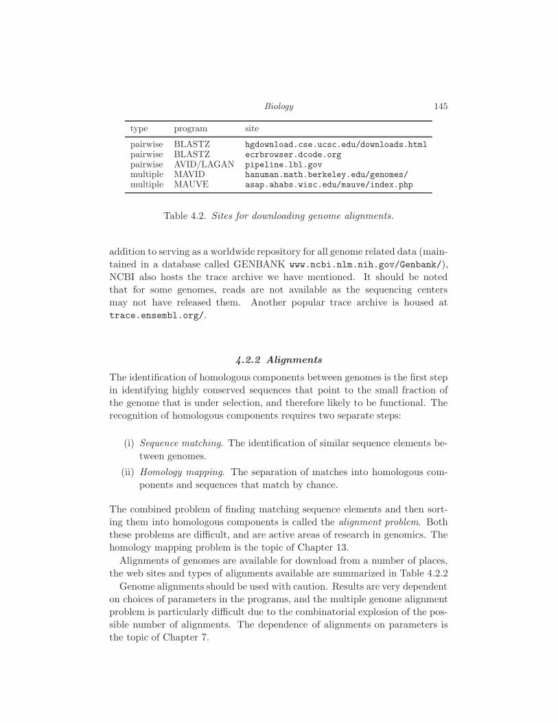
Biology 145
type program site
pairwise BLASTZ hgdownload.cse.ucsc.edu/downloads.htmlpairwise BLASTZ ecrbrowser.dcode.orgpairwise AVID/LAGAN pipeline.lbl.govmultiple MAVID hanuman.math.berkeley.edu/genomes/multiple MAUVE asap.ahabs.wisc.edu/mauve/index.php
Table 4.2. Sites for downloading genome alignments.
addition to serving as a worldwide repository for all genome related data (main-
tained in a database called GENBANK www.ncbi.nlm.nih.gov/Genbank/),
NCBI also hosts the trace archive we have mentioned. It should be noted
that for some genomes, reads are not available as the sequencing centers
may not have released them. Another popular trace archive is housed at
trace.ensembl.org/.
4.2.2 Alignments
The identification of homologous components between genomes is the first step
in identifying highly conserved sequences that point to the small fraction of
the genome that is under selection, and therefore likely to be functional. The
recognition of homologous components requires two separate steps:
(i) Sequence matching. The identification of similar sequence elements be-
tween genomes.
(ii) Homology mapping. The separation of matches into homologous com-
ponents and sequences that match by chance.
The combined problem of finding matching sequence elements and then sort-
ing them into homologous components is called the alignment problem. Both
these problems are difficult, and are active areas of research in genomics. The
homology mapping problem is the topic of Chapter 13.
Alignments of genomes are available for download from a number of places,
the web sites and types of alignments available are summarized in Table 4.2.2
Genome alignments should be used with caution. Results are very dependent
on choices of parameters in the programs, and the multiple genome alignment
problem is particularly difficult due to the combinatorial explosion of the pos-
sible number of alignments. The dependence of alignments on parameters is
the topic of Chapter 7.
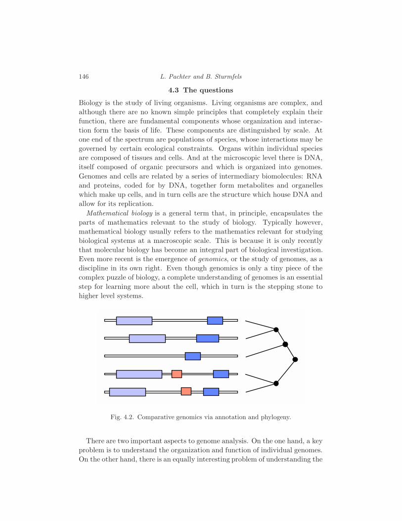
146 L. Pachter and B. Sturmfels
4.3 The questions
Biology is the study of living organisms. Living organisms are complex, and
although there are no known simple principles that completely explain their
function, there are fundamental components whose organization and interac-
tion form the basis of life. These components are distinguished by scale. At
one end of the spectrum are populations of species, whose interactions may be
governed by certain ecological constraints. Organs within individual species
are composed of tissues and cells. And at the microscopic level there is DNA,
itself composed of organic precursors and which is organized into genomes.
Genomes and cells are related by a series of intermediary biomolecules: RNA
and proteins, coded for by DNA, together form metabolites and organelles
which make up cells, and in turn cells are the structure which house DNA and
allow for its replication.
Mathematical biology is a general term that, in principle, encapsulates the
parts of mathematics relevant to the study of biology. Typically however,
mathematical biology usually refers to the mathematics relevant for studying
biological systems at a macroscopic scale. This is because it is only recently
that molecular biology has become an integral part of biological investigation.
Even more recent is the emergence of genomics, or the study of genomes, as a
discipline in its own right. Even though genomics is only a tiny piece of the
complex puzzle of biology, a complete understanding of genomes is an essential
step for learning more about the cell, which in turn is the stepping stone to
higher level systems.
Fig. 4.2. Comparative genomics via annotation and phylogeny.
There are two important aspects to genome analysis. On the one hand, a key
problem is to understand the organization and function of individual genomes.
On the other hand, there is an equally interesting problem of understanding the
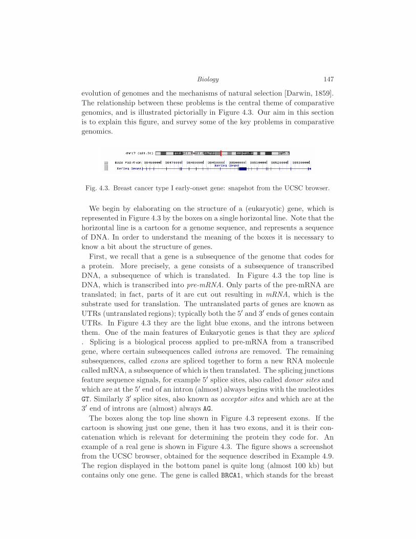
Biology 147
evolution of genomes and the mechanisms of natural selection [Darwin, 1859].
The relationship between these problems is the central theme of comparative
genomics, and is illustrated pictorially in Figure 4.3. Our aim in this section
is to explain this figure, and survey some of the key problems in comparative
genomics.
Fig. 4.3. Breast cancer type I early-onset gene: snapshot from the UCSC browser.
We begin by elaborating on the structure of a (eukaryotic) gene, which is
represented in Figure 4.3 by the boxes on a single horizontal line. Note that the
horizontal line is a cartoon for a genome sequence, and represents a sequence
of DNA. In order to understand the meaning of the boxes it is necessary to
know a bit about the structure of genes.
First, we recall that a gene is a subsequence of the genome that codes for
a protein. More precisely, a gene consists of a subsequence of transcribed
DNA, a subsequence of which is translated. In Figure 4.3 the top line is
DNA, which is transcribed into pre-mRNA. Only parts of the pre-mRNA are
translated; in fact, parts of it are cut out resulting in mRNA, which is the
substrate used for translation. The untranslated parts of genes are known as
UTRs (untranslated regions); typically both the 5′ and 3′ ends of genes contain
UTRs. In Figure 4.3 they are the light blue exons, and the introns between
them. One of the main features of Eukaryotic genes is that they are spliced
. Splicing is a biological process applied to pre-mRNA from a transcribed
gene, where certain subsequences called introns are removed. The remaining
subsequences, called exons are spliced together to form a new RNA molecule
called mRNA, a subsequence of which is then translated. The splicing junctions
feature sequence signals, for example 5′ splice sites, also called donor sites and
which are at the 5′ end of an intron (almost) always begins with the nucleotides
GT. Similarly 3′ splice sites, also known as acceptor sites and which are at the
3′ end of introns are (almost) always AG.
The boxes along the top line shown in Figure 4.3 represent exons. If the
cartoon is showing just one gene, then it has two exons, and it is their con-
catenation which is relevant for determining the protein they code for. An
example of a real gene is shown in Figure 4.3. The figure shows a screenshot
from the UCSC browser, obtained for the sequence described in Example 4.9.
The region displayed in the bottom panel is quite long (almost 100 kb) but
contains only one gene. The gene is called BRCA1, which stands for the breast

148 L. Pachter and B. Sturmfels
s p l i c i n gA T G . . . . . . . . . . . . . . T G At r a n s l a t i o n
t r a n s c r i p t i o ne x o n s i n t r o n s5 ' 3 'D N Ap r e m R N Am R N A p r o t e i n
Fig. 4.4. Structure of a gene.
cancer type I early-onset gene. The top panel shows the location of the region
on chromosome 17. Each of the boxes correspond to an exon. Mutations in
exons of the BRCA1 gene lead to truncated proteins, and studies have con-
firmed that patients with early-onset breast cancer are much more likely than
the general population to have mutations in this gene. One of the interesting
effects of splicing is that may different possible proteins may be coded by a
finite piece of DNA. This can be seen in Example 4.9 by selecting full for the
RefSeq genes which shows different variants of the protein. Mathematically,
the statement that a gene can have many alternative splicings is evident from
the following proposition:
Proposition 4.10 Suppose that a given DNA sequence contains n locations
that could be possible active 5′ splice sites and m locations that could be possible
active 3′ splice sites. In principle, the number of possible gene structures may
be as high as the Fibonacci number Fn+m+1 .
There are many outstanding biology questions related to genes. For example,
it is unknown if there is a functional role for all intronic sequence (sometimes
called “junk” DNA). Furthermore, it is still unclear if there are organizing
principles that explain in simple terms the regulation of genes. The connection
between the gene finding problem and hidden Markov models is explained in
Section 4.4.
Returning to Figure 4.3, we see that the tree on the right hand side shows
the evolutionary relationships between the sequences. This leads us to the
Biology 149
alignment and evolutionary modeling components of comparative genomics.
In order to identify functional elements in the sequences, it is useful to identify
conserved regions in the alignments. Conversely, the alignment problem is
easier if one knows ahead of time the functional elements in each sequence.
Statistical models for alignment and evolutionary models are based on these
biological considerations, and we discuss them in more detail in Section 4.5.
It is important to note that comparative genomics is not only a computa-
tional endeavor. There are many experimental techniques being developed that
can be used to identify functional elements in genomes, and that also shed light
on genome evolution. In this regard it is important to mention the he ENCy-
clopedia of DNA Elements (ENCODE) Project [Consortium, 2004] which is an
NHGRI organized international consortium working towards the goal of identi-
fying all functional elements in the human genome sequence. The pilot phase of
the project is focused on 1% of the human genome sequence. Initial efforts in-
clude the development of high-throughput technologies for detecting functional
elements, as well as the sequencing of orthologous regions from multiple pri-
mates, mammals and other vertebrates. The available sequence from multiple
organisms complements additional sequence extracted from whole genome se-
quencing projects, and serves as a testbed for comparative genomics approaches
to detecting functional elements. Thus, the ENCODE project is aimed at fos-
tering interaction between computational and experimental scientists, and at
identifying promising research avenues and scalable technologies. Preliminary
analysis of some ENCODE regions is discussed in Chapters 22 and 21.
The ENCODE consortium sequence and analysis repository is housed at
genome.ucsc.edu/encode
4.4 Statistical models for a biological sequence
In Chapter 1 we introduced DiaNA, a strange fictional character who flips coins
and generates words on the alphabet A, C, G, T. Although DiaNA does not
seem to have anything to do with real biological DNA sequences, the principle
of imagining DNA to have been generated by fictional entities like DiaNA who
flip coins has proved to be extremely useful for biological sequence analysis. In
order to see this, suppose that we would like to analyze 1 million bases of DNA
from the human genome and identify CpG islands within them. One approach
is to count, for each contiguous subsequence of length 100, the number of Cs
and Gs, and to call a 100bp segment a CpG island if there are more than 70
Cs and Gs. There are a number of problems with such an approach. First,
the segment size 100 is arbitrary; perhaps some biologists prefer working with
segments of length 50, or 200. For such different segment sizes, what should be
the cutoff for deciding when the number of Cs and Gs indicates a CpG island?
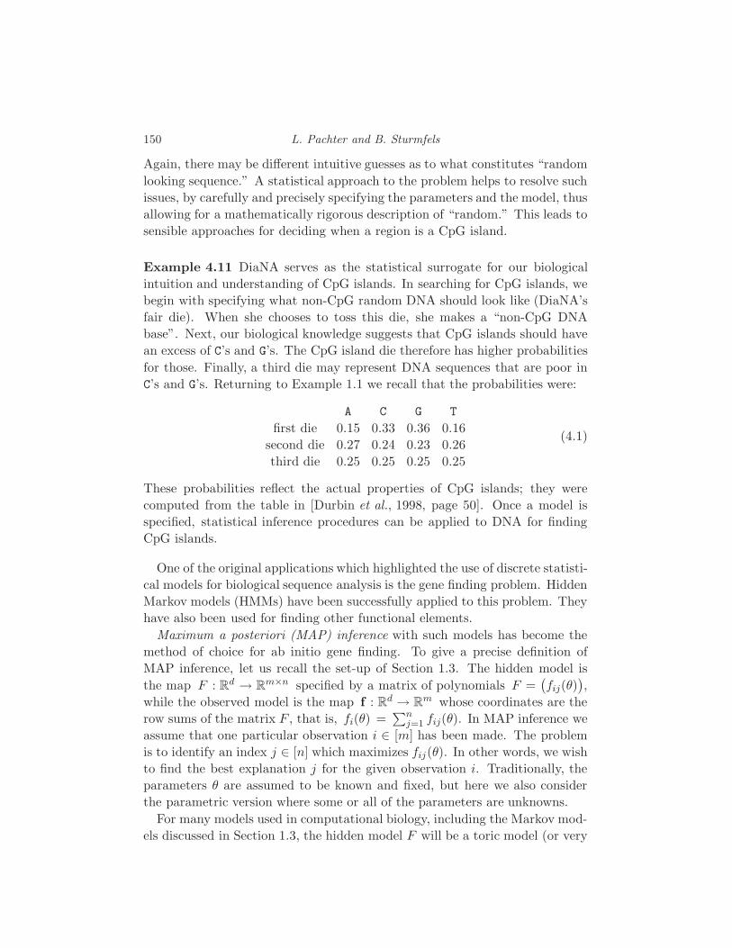
150 L. Pachter and B. Sturmfels
Again, there may be different intuitive guesses as to what constitutes “random
looking sequence.” A statistical approach to the problem helps to resolve such
issues, by carefully and precisely specifying the parameters and the model, thus
allowing for a mathematically rigorous description of “random.” This leads to
sensible approaches for deciding when a region is a CpG island.
Example 4.11 DiaNA serves as the statistical surrogate for our biological
intuition and understanding of CpG islands. In searching for CpG islands, we
begin with specifying what non-CpG random DNA should look like (DiaNA’s
fair die). When she chooses to toss this die, she makes a “non-CpG DNA
base”. Next, our biological knowledge suggests that CpG islands should have
an excess of C’s and G’s. The CpG island die therefore has higher probabilities
for those. Finally, a third die may represent DNA sequences that are poor in
C’s and G’s. Returning to Example 1.1 we recall that the probabilities were:
A C G T
first die 0.15 0.33 0.36 0.16
second die 0.27 0.24 0.23 0.26
third die 0.25 0.25 0.25 0.25
(4.1)
These probabilities reflect the actual properties of CpG islands; they were
computed from the table in [Durbin et al., 1998, page 50]. Once a model is
specified, statistical inference procedures can be applied to DNA for finding
CpG islands.
One of the original applications which highlighted the use of discrete statisti-
cal models for biological sequence analysis is the gene finding problem. Hidden
Markov models (HMMs) have been successfully applied to this problem. They
have also been used for finding other functional elements.
Maximum a posteriori (MAP) inference with such models has become the
method of choice for ab initio gene finding. To give a precise definition of
MAP inference, let us recall the set-up of Section 1.3. The hidden model is
the map F : Rd → Rm×n specified by a matrix of polynomials F =(fij(θ)
),
while the observed model is the map f : Rd → Rm whose coordinates are the
row sums of the matrix F , that is, fi(θ) =∑n
j=1 fij(θ). In MAP inference we
assume that one particular observation i ∈ [m] has been made. The problem
is to identify an index j ∈ [n] which maximizes fij(θ). In other words, we wish
to find the best explanation j for the given observation i. Traditionally, the
parameters θ are assumed to be known and fixed, but here we also consider
the parametric version where some or all of the parameters are unknowns.
For many models used in computational biology, including the Markov mod-
els discussed in Section 1.3, the hidden model F will be a toric model (or very

Biology 151
close to a toric model). This means that the entries of the matrix F are mono-
mials in the parameters, say fij(θ) = θaij for some aij = (aij1, . . . , aijd) ∈ Nd.
Then the probability of observing state i ∈ [m] in the model f equals fi(θ) =∑nj=1 θ
aij . The tropicalization of this polynomial is the tropical polynomial
gi(w) =
n⊕
j=1
w⊙aij = minaij1w1 + aij2w2 + · · ·+ aijdwd
.
If we introduce logarithmic parameters wi = −log(θi) then our problem is to
evaluate the tropical polynomial gi(w). We summarize this as a remark.
Example 4.12 (Google) A useful example to keep in mind when thinking
of MAP inference is the Google “did you mean...” feature. A web search for
the words topicaal geom try leads Google to respond with Did you mean:
tropical geometry. In this case, the observed sequence (or the index i in
the discussion above) is topicaal geom try. The MAP inference problem is
to find the set of words (index j) that maximizes fij(θ). The model can be
specified in many ways, perhaps taking advantage of patterns in the English
language or among commonly used web sites. Below we replace the English
language by DNA, and patterns of usage in the English language by features
of genes.
We emphasize in a separate remark below the connection between MAP infer-
ence and tropical arithmetic. Implications of this connection are discussed in
Chapters 5–9.
Remark 4.13 MAP inference is tropical evaluation of a coordinate polyno-
mial.
In the context of biological sequence analysis, hidden Markov models can be
used to model splice sites of eukaryotic genes. The underlying biology was
explained in the previous section. Our model incorporates two fixed sizes for
the 5′ and 3′ splice sites (k and k′ respectively), and distinguishes exons from
introns. Our HMM has length n where n is the length of the DNA sequences we
wish to model. The alphabet of hidden states is Σ = E, 1, . . . , k, I, 1′, . . . , k′,where E is a state for “exon” sequence preceding the first splice site and I a
state for “intron” after the first splice site. The alphabet of observed states is
Σ′ = A, C, G, T.
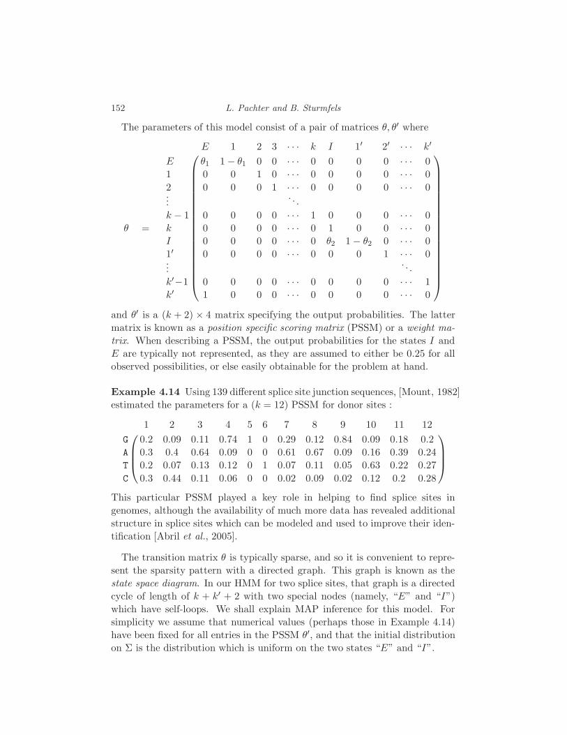
152 L. Pachter and B. Sturmfels
The parameters of this model consist of a pair of matrices θ, θ′ where
θ =
E 1 2 3 · · · k I 1′ 2′ · · · k′
E θ1 1 − θ1 0 0 · · · 0 0 0 0 · · · 0
1 0 0 1 0 · · · 0 0 0 0 · · · 0
2 0 0 0 1 · · · 0 0 0 0 · · · 0...
. . .
k − 1 0 0 0 0 · · · 1 0 0 0 · · · 0
k 0 0 0 0 · · · 0 1 0 0 · · · 0
I 0 0 0 0 · · · 0 θ2 1 − θ2 0 · · · 0
1′ 0 0 0 0 · · · 0 0 0 1 · · · 0...
. . .
k′−1 0 0 0 0 · · · 0 0 0 0 · · · 1
k′ 1 0 0 0 · · · 0 0 0 0 · · · 0
and θ′ is a (k + 2) × 4 matrix specifying the output probabilities. The latter
matrix is known as a position specific scoring matrix (PSSM) or a weight ma-
trix. When describing a PSSM, the output probabilities for the states I and
E are typically not represented, as they are assumed to either be 0.25 for all
observed possibilities, or else easily obtainable for the problem at hand.
Example 4.14 Using 139 different splice site junction sequences, [Mount, 1982]
estimated the parameters for a (k = 12) PSSM for donor sites :
1 2 3 4 5 6 7 8 9 10 11 12
G 0.2 0.09 0.11 0.74 1 0 0.29 0.12 0.84 0.09 0.18 0.2
A 0.3 0.4 0.64 0.09 0 0 0.61 0.67 0.09 0.16 0.39 0.24
T 0.2 0.07 0.13 0.12 0 1 0.07 0.11 0.05 0.63 0.22 0.27
C 0.3 0.44 0.11 0.06 0 0 0.02 0.09 0.02 0.12 0.2 0.28
This particular PSSM played a key role in helping to find splice sites in
genomes, although the availability of much more data has revealed additional
structure in splice sites which can be modeled and used to improve their iden-
tification [Abril et al., 2005].
The transition matrix θ is typically sparse, and so it is convenient to repre-
sent the sparsity pattern with a directed graph. This graph is known as the
state space diagram. In our HMM for two splice sites, that graph is a directed
cycle of length of k + k′ + 2 with two special nodes (namely, “E” and “I”)
which have self-loops. We shall explain MAP inference for this model. For
simplicity we assume that numerical values (perhaps those in Example 4.14)
have been fixed for all entries in the PSSM θ′, and that the initial distribution
on Σ is the distribution which is uniform on the two states “E” and “I”.
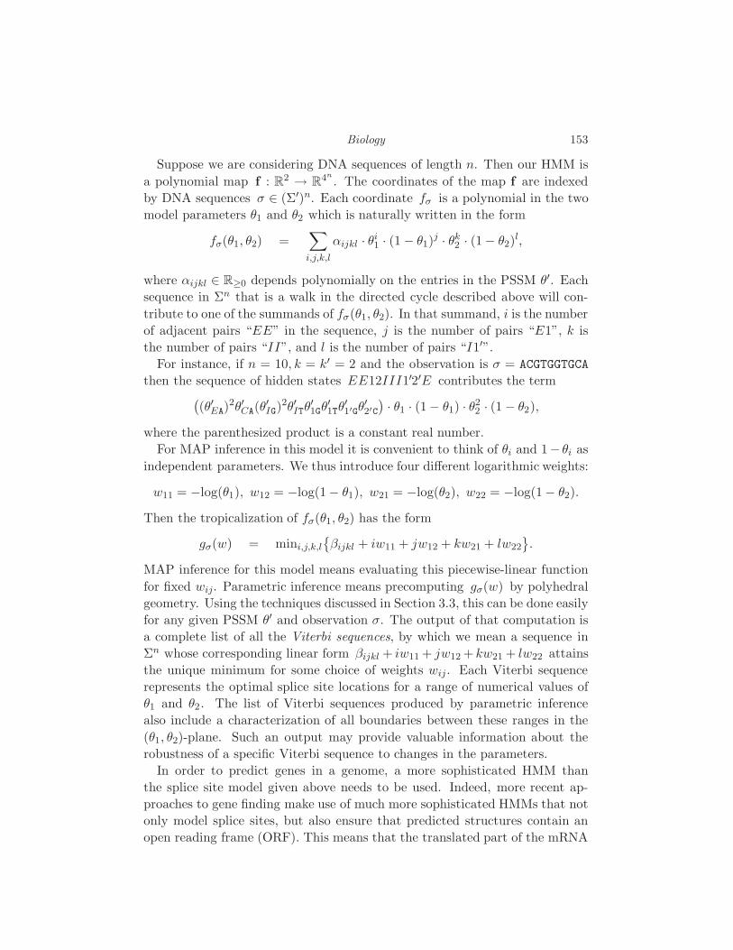
Biology 153
Suppose we are considering DNA sequences of length n. Then our HMM is
a polynomial map f : R2 → R4n. The coordinates of the map f are indexed
by DNA sequences σ ∈ (Σ′)n. Each coordinate fσ is a polynomial in the two
model parameters θ1 and θ2 which is naturally written in the form
fσ(θ1, θ2) =∑
i,j,k,l
αijkl · θi1 · (1 − θ1)
j · θk2 · (1− θ2)
l,
where αijkl ∈ R≥0 depends polynomially on the entries in the PSSM θ′. Each
sequence in Σn that is a walk in the directed cycle described above will con-
tribute to one of the summands of fσ(θ1, θ2). In that summand, i is the number
of adjacent pairs “EE” in the sequence, j is the number of pairs “E1”, k is
the number of pairs “II”, and l is the number of pairs “I1′”.
For instance, if n = 10, k = k′ = 2 and the observation is σ = ACGTGGTGCA
then the sequence of hidden states EE12III1′2′E contributes the term((θ′EA)
2θ′CA(θ′IG)
2θ′ITθ′1Gθ′1Tθ′1′Gθ′2′C
)· θ1 · (1− θ1) · θ22 · (1 − θ2),
where the parenthesized product is a constant real number.
For MAP inference in this model it is convenient to think of θi and 1− θi as
independent parameters. We thus introduce four different logarithmic weights:
w11 = −log(θ1), w12 = −log(1− θ1), w21 = −log(θ2), w22 = −log(1− θ2).
Then the tropicalization of fσ(θ1, θ2) has the form
gσ(w) = mini,j,k,l
βijkl + iw11 + jw12 + kw21 + lw22
.
MAP inference for this model means evaluating this piecewise-linear function
for fixed wij. Parametric inference means precomputing gσ(w) by polyhedral
geometry. Using the techniques discussed in Section 3.3, this can be done easily
for any given PSSM θ′ and observation σ. The output of that computation is
a complete list of all the Viterbi sequences, by which we mean a sequence in
Σn whose corresponding linear form βijkl + iw11 + jw12 + kw21 + lw22 attains
the unique minimum for some choice of weights wij. Each Viterbi sequence
represents the optimal splice site locations for a range of numerical values of
θ1 and θ2. The list of Viterbi sequences produced by parametric inference
also include a characterization of all boundaries between these ranges in the
(θ1, θ2)-plane. Such an output may provide valuable information about the
robustness of a specific Viterbi sequence to changes in the parameters.
In order to predict genes in a genome, a more sophisticated HMM than
the splice site model given above needs to be used. Indeed, more recent ap-
proaches to gene finding make use of much more sophisticated HMMs that not
only model splice sites, but also ensure that predicted structures contain an
open reading frame (ORF). This means that the translated part of the mRNA

154 L. Pachter and B. Sturmfels
must be of length 0 mod 3, and must contain a stop codon only at the very
end. In addition, exon lengths, which are not geometrically distributed, are
modeled explicitly using a modification of hidden Markov models known as
semi-hidden Markov models or generalized HMMs. In Example 4.15 we de-
scribe a model that ensures the correct length for open reading frames, but
that does not explicitly model splice sites or exon lengths. For a descrip-
tion of more complete models see [Burge and Karlin, 1997, Kulp et al., 1996,
Alexandersson et al., 2003, Pachter et al., 2002].
Intron+0 Intron+
1 Intron+2
E+0,2
E+1,1
E+2,0
E+I,0 E+
I,1 E+I,2 E+
0,F E+1,F E+
2,F
Intergene
E−
I,0 E−
I,1 E−
I,2 E−
0,F E−
1,F E−
2,F
E−
1,0E−
1,1
E−
1,2
Intron−
0 Intron−
1 Intron−
2
Fig. 4.5. State space diagram for a simple gene finding HMM.

Biology 155
Example 4.15 [Gene finding HMM] The model consists of a pair of matrices,
θ, θ′, one of which is a 25 × 25 matrix θ (transition probabilities) , and the
other a 25 × 4 matrix (output probabilities). In total, there can therefore be
up to 725 parameters. In practice, biological considerations simplify matters,
leading to matrices θ that are very sparse. In fact, the specific model we have
in mind has only 41 non-zero entries for the matrix θ. There is also additional
structure in θ, for example many entries are set to 1. Models with so many
parameters are summarized with a state transition diagram (see Figure 4.5).
The state transition diagram is a graph with one node for every state in Σ.
There is an edge for every nonzero entry in the matrix θ. Notice that the
bottom half of the state transition diagram is a mirror image of the top half
(with the directions of the arrows reversed). This reflects the fact that genes
can be found on either strand of the DNA sequence.
Proposition 4.16 The probability of any hidden path in the model in Example
4.15 that does not use 0 mod 3 exon states is 0.
The parameters θ′ in a gene finding HMM are derived from known observed
frequencies of codons in known genes, and from the overall frequencies of the
bases in intergenic and intronic DNA. In other words, the maximum likelihood
estimates for these parameters can be obtained from the fully observed model
using Proposition 1.9 and Theorem 1.10. The parameters in θ relate biologi-
cally to lengths of introns, exons, and the distance between genes. These are
also derived from known genes (for how this is done see the final section below).
In principle, one could estimate the parameters using MLE with the hidden
model, however this is typically not done in practice.
The model we have described in Example 4.15 has a number of limitations.
As we have discussed, it does not model splice sites at all and there is no
explicit modeling of exon lengths. There are also other gene elements that
are simply not possible to model at all with current methods. For example,
different cell types in an organism have different genes transcribed (and there-
fore translated) at different times. This process is largely regulated through
enhancement or suppression of transcription, and is referred to as regulation.
Transcription factor binding sites (TFBS), also called cis-regulatory elements
are small sequences, typically in the neighborhood of genes that are bound
to by proteins that mediate transcription (called trans-acting). A complete
solution to the gene finding problem therefore requires annotation of TFBSs.
Despite some encouraging results for TFBS identification with hidden Markov
models, the problem problem is much harder and has traditionally been tackled
separately.

156 L. Pachter and B. Sturmfels
4.5 Statistical models of mutation
Point mutations in DNA sequences are well modeled by continuous Markov pro-
cesses on trees. This point of view, pioneered by Joe Felsenstein [Felsenstein, 2003],
has been extensively explored and developed during the past thirty years. The
relevant algebraic statistics involves the hidden tree models of Subsection 1.4.4.
In what follows we offer a derivation of biologically relevant hidden tree models.
We also return to our discussion of pair hidden Markov models for sequence
alignment, with a biological discussion of insertions and deletions, and by ex-
plaining what exactly DiaNA is doing in the diagram on the book cover.
4.5.1 Evolutionary Models
Although the biology of point mutation is complicated, the use of Markov
processes on trees is motivated by underlying principles which capture, to
some degree, the complexities of mutation. These are:
• Mutations occur at random, although possibly with different probabilities
at different places in the genome.
• Mutations occur independently in different species.
• In genome locations where mutations can occur, there is, at any given time,
a nonzero probability that mutation occurs.
The first two requirements leads naturally to hidden tree models. The tree
T corresponds to a species tree, with different species labeling the leaves of the
tree. Thus, we have the structure of a phylogenetic tree appearing naturally,
and associating a hidden tree model with the point mutation process is equiv-
alent to specifying that bases observed at the leaves of the tree are a result of
a stochastic process of mutation between “hidden” interior vertices of the tree.
The third requirement leads to a further restriction of hidden tree models,
specifically to evolutionary models . We now define this class of models.
A rate matrix (or Q-matrix) is a square matrix Q = (qij)i,j∈Σ, with rows
and columns indexed by Σ = A, C, G, T (note that the twenty letter alphabet
of amino acids may also be used). Rate matrices must satisfy the following
requirements:
qij ≥ 0 for i 6= j,
∑
j∈Σ
qij = 0 for all i ∈ Σ,
qii < 0 for all i ∈ Σ.

Biology 157
Rate matrices capture the notion of instantaneous rate of mutation. From a
given rate matrix Q one computes the substitution matrices θ(t) by exponen-
tiation. The entry of θ(t) in row i and column j equals the probability that
the substitution i→ · · · → j occurs in a time interval of length t.
Theorem 4.17 Let Q be any rate matrix and θ(t) = eQt =∑∞
i=01i !Q
iti. Then
(i) θ(s+ t) = θ(s) · θ(t) (Chapman-Kolmogorov equations),
(ii) θ(t) is the unique solution to the forward differential equation
θ′(t) = θ(t) ·Q, θ(0) = 1 for t ≥ 0, (here 1 is the identity matrix)
(iii) θ(t) is the unique solution to the backward differential equation
θ′(t) = Q · θ(t), θ(0) = 1 for t ≥ 0.
(iv) θ(k)(0) = Qk.
Furthermore, a matrix Q is a rate matrix if and only if the matrix θ(t) = eQt is
a stochastic matrix (nonnegative with row sums equal to one) for every t ≥ 0.
Proof For any matrix A, the matrix exponential eA is defined by
eA :=
∞∑
k=0
Akk
k!.
The matrix exponential is well defined because the series on the right hand side
converges componentwise for any A. A standard identity that can be derived
directly from the definition is that eA+B = eAeB provided that A and B are
matrices that commute. Since sQ and tQ commute for any s, t, it follows that
θ(s + t) = θ(s) · θ(t). In order to derive (ii) and (iii), we need to differentiate
θ(t) term-by-term, which is possible because the power series θ(t) has infinite
radius of convergence. We find that
θ′(t) =∞∑
k=1
tk−1Qk
(k − 1)!= θ(t) ·Q = Q · θ(t).
Iterated differentiation leads to the identity (iv), which says that the kth deriva-
tive of θ(t) evaluated at 0 is just the matrix Qk. The uniqueness in parts (ii)
and (iii) is a standard result on systems of ordinary linear differential equations.
The last part of the theorem provides the crucial connection between rate
matrices and substitution matrices. One direction of the theorem is easy: if
θ(t) is a substitution matrix for every t ≥ 0, then∑
j θij(t) = 1 for all t ≥ 0.
Using identity (iv) with k = 1, we have that∑
j
qij(t) =∑
j
θ′ij(0) = 0.
This says that the row sums of Q are 0, i.e., Q is a rate matrix. To prove

158 L. Pachter and B. Sturmfels
the other direction, we note that as t → 0, the Taylor series expansion gives
θ(t) = I+tQ+O(t2) which immediately implies that qij(t) ≥ 0 for i 6= j if and
only if θij(t) ≥ 0 for all i, j when t is sufficiently small. But θ(t) = θ(t/m)m
for all m, so in fact qij ≥ 0 iff θij(t) ≥ 0 for all t ≥ 0. Finally, it is easy to
check that since Q has row sums equal to zero, so does Qm for all m, and so
the result follows directly from the definition of θ(t) in terms of Q.
A standard example is the Jukes-Cantor rate matrix
Q =
−3α α α α
α −3α α α
α α −3α α
α α α −3α
,
where α ≥ 0 is a parameter. The corresponding substitution matrix equals
θ(t) =1
4
1 + 3e−4αt 1 − e−4αt 1 − e−4αt 1 − e−4αt
1 − e−4αt 1 + 3e−4αt 1 − e−4αt 1 − e−4αt
1 − e−4αt 1 − e−4αt 1 + 3e−4αt 1 − e−4αt
1 − e−4αt 1 − e−4αt 1 − e−4αt 1 + 3e−4αt
.
The expected number of substitutions over time t is the quantity
3αt = −1
4· trace(Q) · t = −1
4· log det
(θ(t)
). (4.2)
This number is called the branch length. It can be computed from the substi-
tution matrix θ(t) and is used to weight the edges in a phylogenetic tree.
One way to specify an evolutionary model is to give a phylogenetic tree T
together with a rate matrix Q and an initial distribution for the root of T
(which we here assume to be the uniform distribution on Σ). The branch
lengths of the edges are unknown parameters, and the objective is to estimate
these branch lengths from data. Thus if the tree T has r edges, then such
a model has r free parameters, and, according to the philosophy of algebraic
statistics, we would like to regard it as an r-dimensional algebraic variety.
Such an algebraic representation does indeed exist, This is not entirely obvi-
ous since the probabilities in the substitution θ(t) do not depend polynomially
on the parameters α and t. We shall explain the (algebraic representation of)
the Jukes-Cantor DNA model on an arbitrary finite rooted tree T . Suppose
that T has r edges and the leaves are indexed by [n] = 1, 2, . . . , n. Let θi(t)
denote the substitution matrix associated with the i-th edge of the tree.
We make the following change of variables in the space of parameters. In-
stead of using αi and ti as in (4.2), we introduce the new two parameters
πi =1
4(1 − e−4αiti) and µi =
1
4(1 + 3e−4αiti).
Biology 159
These parameters satisfy the linear constraint
µi + 3πi = 1,
and the branch length of the i-th edge can be recovered as follows:
3αiti = −1
4· log det
(θi)
= −3
4· log(1− 4πi).
Indeed, the parameters are simply the entries in the substitution matrix
θi =
µi πi πi πi
πi µi πi πi
πi πi µi πi
πi πi πi µi
.
The Jukes-Cantor model is a submodel of the general Hidden Tree Model
which was introduced in Section 1.4. Namely, the Jukes-Cantor model on the
tree T with r edges and n leaves is the polynomial map
f : Rr → R4n
which is obtained by specializing the transition matrices to the specific 4 × 4
matrices θi above.
Remark 4.18 Each coordinate polynomial fu1u2···un of the Jukes-Cantor model
is a multilinear polynomial in the model parameters (µ1, π1), . . . , (µn, πn), i.e.,
fu1u2···un is linear in (µi, πi) when the other parameters are fixed.
As an illustration we derive the model which was featured in Example 1.7.
Example 4.19 Let n = r = 3, and let T be the tree with three leaves, labeled
by 1, 2, 3, directly branching off the root of T . We consider the Jukes-
Cantor DNA model with uniform root distribution on T . This model is a
three-dimensional algebraic variety, given as the image of a trilinear map
f : R3 → R64.
The number of states in A, C, G, T3 is 43 = 64 but there are only five distinct
polynomials occurring among the coordinates of the map f . Let p123 be the
probability of observing the same letter at all three leaves, pij the probability
of observing the same letter at the leaves i, j and a different one at the third
160 L. Pachter and B. Sturmfels
leaf, and pdis the probability of seeing three distinct letters. Then
p123 = µ1µ2µ3 + 3π1π2π3,
pdis = 6µ1π2π3 + 6π1µ2π3 + 6π1π2µ3 + 6π1π2π3,
p12 = 3µ1µ2π3 + 3π1π2µ3 + 6π1π2π3,
p13 = 3µ1π2µ3 + 3π1µ2π3 + 6π1π2π3,
p23 = 3π1µ2µ3 + 3µ1π2π3 + 6π1π2π3.
All 64 coordinates of f are given by these five trilinear polynomials, namely,
fAAA = fCCC = fGGG = fTTT =1
4· p123,
fACG = fACT = · · · = fGTC =1
24· pdis,
fAAC = fAAT = · · · = fTTG =1
12· p12,
fACA = fATA = · · · = fTGT =1
12· p13,
fCAA = fTAA = · · · = fGTT =1
12· p23.
This means that our Jukes-Cantor model is the image of the simplified map
f ′ : R3 → R5,((µ1, π1), (µ2, π2), (µ3, π3)
)7→ (p123, pdis, p12, p13, p23).
There are only three parameters since µi+3πi = 1. Algebraists prefer the above
representation with (µi : πi) as homogeneous coordinates on the projective line.
To characterize the image of f ′ algebraically, we perform the following linear
change of coordinates:
q111 = p123 + 13pdis − 1
3p12 − 13p13 − 1
3p23 = (µ1 − π1)(µ2 − π2)(µ3 − π3)
q110 = p123 − 13pdis + p12 − 1
3p13 − 13p23 = (µ1 − π1)(µ2 − π2)(µ3 + 3π3)
q101 = p123 − 13pdis − 1
3p12 + p13 − 13p23 = (µ1 − π1)(µ2 + 3π2)(µ3 − π3)
q011 = p123 − 13pdis − 1
3p12 − 13p13 + p23 = (µ1 + 3π1)(µ2 − π2)(µ3 − π3)
q000 = p123 + pdis + p12 + p13 + p23 = (µ1 + 3π1)(µ2 + 3π2)(µ3 + 3π3)
This reveals that our model is the hypersurface in ∆4 whose ideal equals
IT = 〈 q000q2111 − q011q101q110 〉
If we set µi = 1 − 3πi then we get the additional constraint q000 = 1.
The construction in this example generalizes to arbitrary trees T . There ex-
ists a change of coordinates, simultaneously on the parameter space (P1)r and
on the probability space P4n−1, such that the map f becomes a monomial map in
Biology 161
the new coordinates. This change of coordinates is known as the Fourier trans-
form or as the Hadamard conjugation (see [Evans and Speed, 1993, Hendy and Penny, 1993,
Semple and Steel, 2003]).
We regard the Jukes-Cantor DNA model on a tree T with n leaves and r
edges as an algebraic variety of dimension r in P4n−1, namely, it is the image
of the map f . Its homogeneous prime ideal IT is generated by differences of
monomials qa − qb in the Fourier coordinates. In the phylogenetics literature
(including the books [Felsenstein, 2003, Semple and Steel, 2003]), the polyno-
mials in the ideal IT are known as phylogenetic invariants of the model. The
following result was shown in [Sturmfels and Sullivant, 2004].
Theorem 4.20 The ideal IT which defines the Jukes-Cantor model on a bi-
nary tree T is generated by monomial differences qa − qb of degree at most
three.
If we allowQ to be an arbitrary rate matrix then P (t) is an arbitrary stochas-
tic matrix. The resulting model is the general Markov model on the tree T . All-
man and Rhodes [Allman and Rhodes, 2003] determined an almost-complete
system of phylogenetic invariants for the general Markov model on a tree T .
An important problem in phylogenomics is to identify the maximum like-
lihood branch lengths, given a phylogenetic X-tree T , a rate matrix Q and
an alignment of sequences. For the Jukes-Cantor DNA model on three taxa,
described in Example 4.19, the exact “analytic” solution of this optimization
problem leads to an algebraic equation of degree 23. See Section 3.3 for details.
The Felsenstein hierarchy is the cumulative result of experimentation and
development of many special continuous time Markov models with rate ma-
trices that incorporate biologically meaningful parameters. The models are
summarized in Figure 4.6, with arrows indicating the nesting of the models,
and the more general models on top. Each matrix shown is a rate matrix Q,
and it is assumed that πA + πC + πG + πT = 1. The diagonal entries (marked
by a dot) are forced, by the definition of a rate matrix, to equal the negative
of the sum of the other entries in their row.
The simplest model is the Jukes-Cantor model [Jukes and Cantor, 1969]
which is highly structured and imposes a uniform root distribution, together
with equal probabilities for transitions and transversions. On the other end of
the spectrum is the general time reversible (REV) model which only imposes
the requirement of time reversibility. The drawback of the REV model is that
it lacks the group structure of the Jukes-Cantor model, and maximum likeli-
hood estimation is also complicated by the added parameters. A number of
compromises have been studied, one of the most popular being the Hasegawa-
Kishino-Yano (HKY) model. This model allows for different transition and
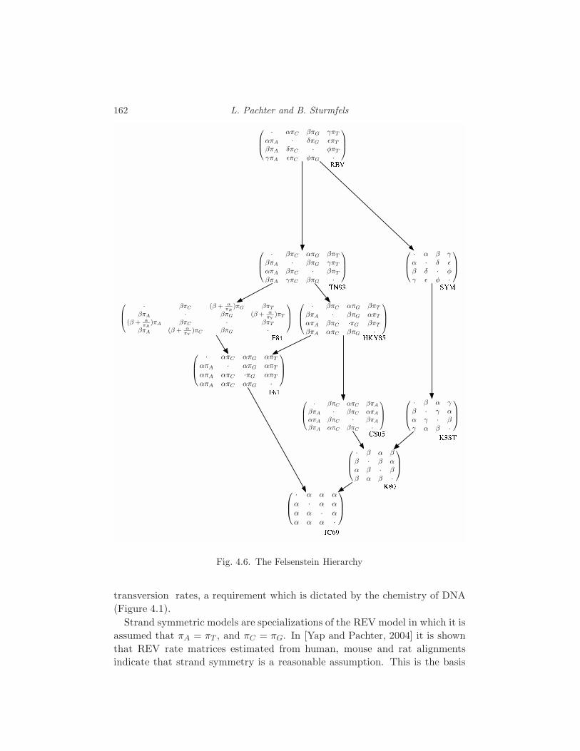
162 L. Pachter and B. Sturmfels
J C 6 9 K 8 0F 8 1
H K Y 8 5
· απC απG απT
απA · απG απT
απA απC ·πG απT
απA απC απG ·
· α α α
α · α α
α α · α
α α α ·
· βπC απG βπT
βπA · βπG απT
απA βπC ·πG βπT
βπA απC βπG ·
F 8 4
R E V
K 3 S T
S Y M
· βπC (β + α
πR
)πG βπT
βπA · βπG (β + α
πY
)πT
(β + α
πR
)πA βπC · βπT
βπA (β + α
πY
)πC βπG ·
· βπC απC βπA
βπA · βπC απA
απA βπC · βπA
βπA απC βπC ·
C S 0 5
· β α β
β · β α
α β · β
β α β ·
T N 9 3
· α β γ
α · δ ǫ
β δ · φ
γ ǫ φ ·
· β α γ
β · γ α
α γ · β
γ α β ·
· απC βπG γπT
απA · δπG ǫπT
βπA δπC · φπT
γπA ǫπC φπG ·
· βπC απG βπT
βπA · βπG γπT
απA βπC · βπT
βπA γπC βπG ·
Fig. 4.6. The Felsenstein Hierarchy
transversion rates, a requirement which is dictated by the chemistry of DNA
(Figure 4.1).
Strand symmetric models are specializations of the REV model in which it is
assumed that πA = πT , and πC = πG. In [Yap and Pachter, 2004] it is shown
that REV rate matrices estimated from human, mouse and rat alignments
indicate that strand symmetry is a reasonable assumption. This is the basis
Biology 163
for the study of the strand symmetric model in Chapter 16 by Casanellas and
Sullivant.
We conclude with two examples: one that shows how mutation models are
used in distance based tree reconstruction methods, and another which illus-
trates the use of evolutionary models for identifying conserved positions in
genomes.
Example 4.21 (Jukes-Cantor correction) Suppose that we are given a
multiple alignment from which we would like to infer a tree:
Human: ACAATGTCATTAGCGAT . . .
Mouse: ACGTTGTCAATAGAGAT . . .
Rat: ACGTAGTCATTACACAT . . .
Chicken: GCACAGTCAGTAGAGCT . . .
If there are many taxa, it is not feasible to search through all trees (Section
2.4), so instead a metric is constructed and then projected onto a tree metric.
The neighbor joining algorithm 2.40 is the most widely used projection.
In order to obtain a metric, mutation models are used to compute the max-
imum likelihood distance between each pair of taxa. In the case of the Jukes-
Cantor model this is known as the Jukes-Cantor correction. More generally,
such estimates are called pairwise distance estimates. Here the tree T has only
two leaves, labeled by X = 1, 2, directly branching off the root of T . The
model is given by a surjective bilinear map
φ : P1 × P1 → P1 , ((µ1, π1), (µ2, π2)) 7→ ( p12, pdis ). (4.3)
The coordinates of the map φ are
p12 = µ1µ2 + 3π1π2,
pdis = 3µ1π2 + 3µ2π1 + 6π1π2.
As before, we pass to affine coordinates by setting µi = 1 − 3πi for i = 1, 2.
One crucial difference between the model (4.3) and Example 4.19 is that
the parameters in (4.3) are not identifiable. Indeed, the inverse image of any
point in P1 under the map φ is a curve in P1×P1. Suppose we are given data
consisting of two aligned DNA sequences of length n where k of the bases are
different. The corresponding point in P1 is u = (n− k, k). The inverse image
of u under the map φ is the curve in the affine plane with the equation
12nπ1π2 − 3nπ1 − 3nπ2 + k = 0.
Every point (π1, π2) on this curve is an exact fit for the data u = (n − k, k).
Hence this curve equals the set of all maximum likelihood parameters for this

164 L. Pachter and B. Sturmfels
model and the given data. We rewrite the equation of the curve as follows:
(1 − 4π1)(1 − 4π2) = 1− 4k
3n. (4.4)
Recall from (4.2) that the branch length from the root to leaf i equals
3αiti = −1
4· log det
(θi(t)
)= −3
4· log(1− 4πi).
By taking logarithms on both sides of (4.4), we see that the curve of all maxi-
mum likelihood parameters becomes a line in the branch length coordinates:
3α1t1 + 3α2t2 = −3
4· log
(1 − 4k
3n
). (4.5)
The sum on the left hand side equals the distance from leaf 1 to leaf 2 in the
tree T . We summarize our discussion of the two-taxa model as follows:
Proposition 4.22 Given an alignment of two sequences of length n, with k
differences between the bases, the ML estimate of the branch length equals
δ12 = −3
4· log
(1 − 4k
3n
).
Similar results exist for other models in the Felsenstein hierarchy.
Example 4.23 (Phylogenetic shadowing) Suppose we are given a column
in a multiple alignment and we would like to know whether it is conserved or
not. One way to answer this question is to perform a likelihood ratio test with
two different points on an evolutionary model. That is, for a fixed observation
σ = σ1σ2 · · ·σn of nucleotides at the leaves of a tree T , for a fixed model in the
hierarchy, and for two different rate matrices QS (slow model) and QF (fast
model), we compute
log pFσ
log pSσ
(4.6)
where pFσ is the probability of σ with rate matrix QF , and pS
σ is the probability
of σ with rate matrix QS. Such a test is especially sensible if the species be-
ing compared to each are at nearby evolutionary distances, so that the multiple
alignment is reliable without many insertions and deletions [Boffelli et al., 2003].
Phylogenetic hidden Markov models are extensions of hidden Markov models
to more general tree models that take advantage of this idea. More details can
be found in [Siepel and Haussler, 2004, McAuliffe et al., 2004].
Biology 165
4.5.2 Insertion and Deletion
One of the main mechanisms by which DNA sequences change is insertion and
deletion. Insertions and deletions can happen, for example, during DNA repli-
cation. Repetitive sequences are particularly prone to a phenomenon known as
strand slippage, during which non-pairing of the complementary strand results
in small insertions or deletions [Levinson and Gutman, 1987]. In order to cor-
rectly align sequences, it is therefore necessary to accurately model insertions
and deletion, as well as point mutation.
The description of how pair hidden Markov models are parameterized based
on biological considerations and subsequently used for inference takes us back
to DiaNA, and her picture on the cover of the book. DiaNA is again our
surrogate for biological intuition, and what follows is an exact description of
what she is doing:
Example 4.24 (DiaNA hopping on the alignment graph) The graph on
which DiaNA walks is the alignment graph Gn,m (Section 2.2). This is a square
grid which includes diagonal edges. DiaNA begins at one corner and will walk
along edges of the graph until she reaches the opposite corner. She must always
walk towards the far corner; so in particular she cannot backtrack her steps.
She walks randomly, which means that at every vertex, she decides at random
which of the three directions to take. When she is on a boundary however,
she is constrained to walk in only one direction since she must always progress
towards the far corner.
Each time she takes a step she crosses an edge, and as she does so she tosses
two tetrahedral die. Each of these die has the letters A,C,G,T written on the
four sides. The die land (at random) and we, the result is recorded for us, the
observers. Unfortunately, we are blindfolded so we cannot see DiaNA as she
hops along the graph, but fortunately, her tetrahedral die tosses are recorded
for us and we read them after she is done hopping. Our gaol is to guess which
path she took on the graph.
Recall from Chapter 2 that a pair hidden Markov model is specified by two
matrices, θ and θ′. DiaNA’s random walk on the graph is determined by the
matrix θ′. It is therefore theta′ which models insertions and deletions, with
the probabilities associated to the length distributions. Suppose that DiaNA
makes an insertion move. The probability that she repeats an insertion is θ′I,I .
It follows that the probability that she remains walking in the same direction
(i.e., keeps making insertions) for k steps is therefore (θ′I,I)k. The insertions
generated by DiaNA are therefore geometrically distributed in length, with
expected length 11−(θ′I,I )k . The average length of observed insertions and dele-
tions can therefore be used to set the parameters θ′I,I and θ′D,D. Similarly, the

166 L. Pachter and B. Sturmfels
frequency of insertions and deletions determines the parameters θ′H,I and θ′H,D.
Unfortunately, to date there has not been enough data to carefully measure
these quantities, however it should be possible in the near future thanks to the
extraordinary amount of new sequence data, much of it from closely related
species pairs.
DiaNA’s pair hidden Markov model also consists of a matrix θ, which con-
tains the probabilities for pairs of nucleotides. It is therefore necessary to select
a model for mutation, and to this end the models described in the point mu-
tation section are very reasonable. Thus, DiaNA’s pair hidden Markov model
contains an evolutionary model as an ingredient (albeit with two taxa in the
case of pairwise sequence alignment).
In Chapter 7, the question is explored of whether pair hidden Markov models
are sufficient for modeling insertion and deletion. In particular, it is shown
that there are genomic sequences for which no choice of parameters yields the
correct alignment, thus indicating that there is lots of room for improvement
in the modeling of sequences and their mutations. In other words, we do not
yet understand exactly what it is that DiaNA is doing.
Our goal, of which we must not lose sight, is to find the best alignment, which
means guessing how DiaNA hopped along the graph. Recalling Remark 4.13
this is precisely MAP inference, which is the tropical evaluation of a coordinate
polynomial of the model.

Part II
Studies on the four themes
The contributions in this part of the book were all written by students,
postdocs and visitors who in some way were involved in the graduate course
Algebraic Statistics for Computational Biology that we taught in in the mathe-
matics department at UC Berkeley during the fall of 2004. The chapters range
in scope from specialized case studies, further developing some of the themes
in Part 1, to full-blown research article on topics of current interest.
Many of the eighteen chapters contain original research that has not been
published elsewhere. Some of the highlights among new results include:
• Theorem 6.7 which states that polytope propagation on a graph runs in
polynomial time, even if the number of parameters is not fixed (Chapters
6). This is accompanied by theoretical investigations into exact bounds
(Chapter 8) and the impact of specializing parameters (Chapter 5).
• An example of a biologically correct alignment which is not the optimal
alignment for any choice of parameters in the pair HMM (Chapter 7).
• Theorem 9.1 which states that the number of inference functions of a graph-
ical model grows polynomially for fixed number of parameters.
• Theorem 10.5 which states that, for alphabets with four or more letters,
every toric Viterbi sequence is a Viterbi sequence.
• Explicit calculations of phylogenetic invariants for the strand symmetric
model (Chapter 16) which highlight connections between the general re-
versible model and group based models.
• A novel method for tree reconstruction based on singular value decomposi-
tion (Chapter 19).
The other chapters also include either interesting new results, or in some
cases important methodological advances. Chapter 15 introduces a standard-
ized framework for working with small trees. Even results on the smallest non-
trivial tree (with three leaves) are interesting, and are discussed in Chapter 18.
Similarly, Chapter 14 presents a unified algebraic statistical view of mutagenic
tree models. In terms of tools, Chapters 11 and 20 describe novel numerical
approaches to solving long-standing problems. Chapter 12 is a thorough ex-
position of the Baum-Welch algorithm, and addresses some of the pitfalls to
beware of when applying it. Chapters 13, 21 and 22 focus on some of the
immediate challenges we face in working with and interpreting genomic data.

168
We present a brief biography for each of our twenty-seven contributors that
summarizes their backgrounds, and explains their connection to our class.
• Jameel Al-Aidroos is a Ph.D. student in mathematics at UC Berkeley.
He has worked on algebraic geometry (supervised by Tom Graber), and was
first introduced to computational biology during our course in fall 2004.
• Niko Beerenwinkel received his Ph.D. in computer science in 2004 from
the University of Saarbrucken, Germany (supervised by Thomas Lengauer).
His thesis was on computational biology using machine learning methods.
Upon graduation, he was awarded the prestigious Emmy Noether fellowship
which he is using to pursue postdoctoral research at UC Berkeley.
• Nicolas Bray graduated with a B.S. in mathematics from UC Berkeley
in 2004, and continues now as a Ph.D. student in the same department
(supervised by Lior Pachter). He is the developer of the MAVID multiple
alignment program, and continues to work on comparative genomics.
• David Bryant is an assistant professor of mathematics and computer sci-
ence at McGill University in Montreal, Canada, and also holds a faculty
position at the University of Auckland, New Zealand. An expert on phylo-
genetic analysis, he is a co-developer of the software package SplitsTree.
David Bryant was invited to lecture in our course during the fall of 2004.
• Marta Casanellas is an assistant professor at the Universitat Politecnica
de Catalunya in Barcelona, Spain. She is an expert in algebraic geometry,
and became interested in computational biology in 2004, in the course of
visiting Roderic Guigo and his computational biology group at the Institut
Municipal d’Investigacio Medical in Barcelona. Marta came to Berkeley in
the fall of 2004 for an extended visit, and now works on phylogenetics.
• Anat Caspi is a Ph.D. student in the joint UC San Francisco/UC Berkeley
graduate group in bioengineering (supervised by Lior Pachter). She has a
Masters degree in computer science from Stanford University, and is inter-
ested in machine learning applications to computational biology.
• Mark Contois is an undergraduate student in mathematics at San Fran-
cisco State University (supervised by Serkan Hosten). He has also working
on computational biology in the laboratory of Eric Routman.
• Colin Dewey studied biology and computer science as an undergraduate
at UC Berkeley, and is now a Ph.D. student in computer science (supervised
by Lior Pachter). He has worked on homology mapping and parametric
sequence alignment, and is the developer of the Mercator mapping program.
• Mathias Drton received his Ph.D. in statistics from the University of Wash-
ington in 2004 (supervised by Michael Perlman and Thomas Richardson).
He has worked on maximum likelihood estimation in graphical models, and
is a postdoctoral researcher at UC Berkeley. In Fall 2005 he will start a

169
tenure track position in the Department of Statistics at the University of
Chicago.
• Sergi Elizalde received his Ph.D. in applied mathematics from M.I.T. in
2004 (supervised by Richard Stanley) where he worked on combinatorics
and enumeration. He is currently a postdoctoral fellow at the Mathematical
Sciences Research Institute at Berkeley (MSRI). Starting in Fall 2005, he
will be a John Wesley Instructor in Mathematics at Dartmouth College.
• Nicholas Eriksson is a Ph.D. student in mathematics at UC Berkeley
(supervised by Bernd Sturmfels). He has worked on on algebraic statistics
and is the first mathematics graduate student at UC Berkeley to enroll in the
designated emphasis in computational biology interdisciplinary program.
• Luis David Garcia received his Ph.D. in mathematics from Virginia Poly-
technic Institute in 2004 (supervised by Reinhard Laubenbacher), where he
worked at the Virginia Bioinformatics Institute. After spending a postdoc-
toral semester in the fall 2004 program on Hyperplane Arrangements at
MSRI, he is now a Visiting Assistant Professor at Texas A & M University.
• Ingileif B. Hallgrımsdottir will receive her Ph.D. in statistics from UC
Berkeley in June 2005 (supervised by Terence Speed). She works in sta-
tistical genetics, a topic which she had already pursued while working at
DeCODE Genetics in Iceland, and for her Masters in Gothenburg, Sweden.
• Michael Joswig is an expert in mathematical software and polyhedral ge-
ometry. He developed the software POLYMAKE. Michael holds a professorship
in Mathematics at the Technische Universitat Darmstadt, Germany.
• Eric Kuo will receive his Ph.D. in computer science from UC Berkeley in
June 2005 (supervised by Lior Pachter). His interests range from theoretical
computer science to convex polytopes and discrete mathematics.
• Fumei Lam will receive her Ph.D. in applied mathematics from M.I.T.
in June 2005 (supervised by Michel Goemans). She has worked on graph
theory, approximation algorithms and computational biology.
• Garmay Leung is a Ph.D. student in the joint UC San Francisco/UC
Berkeley graduate group in bioengineering and is doing rotations (currently
with Michael B. Eisen). She did research on computational biology and cell
biology as an undergraduate at Cornell University.
• Dan Levy is receiving his Ph.D. in mathematics during the summer of 2005
(supervised by Lior Pachter and Rainer Sachs), and will stay in Berkeley for
one more postdoctoral year. His research is in mathematical biology.
• Radu Mihaescu has a B.A. from Princeton University and is now a Ph.D.
student in mathematics at UC Berkeley (supervised by Lior Pachter and
Satish Rao). He is interested in theoretical computer science.
• Alex Milowski received his M.A. in mathematics from San Francisco State
University in May 2004 (supervised by Serkan Hosten). He was one of the

170
developers of the Extensible Markup Language (XML) and related stan-
dards.
• Jason Morton is a second-year Ph.D. student in mathematics at UC Berke-
ley (supervised by Bernd Sturmfels). He is interested in algebraic statistics.
• Raazesh Sainudiin will receive his Ph.D. in statistics from Cornell Univer-
sity in May 2005 (supervised by Rick Durett). His research is on statistical
inference in population penetics, phylogenetics and molecular evolution.
• Sagi Snir received his Ph.D. in computer science in May 2004 from the
Technion - Israel Institute of Technology (supervised by Benny Chor). He
has worked on analytic maximum likelihood solutions for phylogenetic re-
construction, and on convex recoloring. He is a postdoc at UC Berkeley.
mathematics department at UC Berkeley.
• Seth Sullivant received his M.A. from San Francisco State University in
2002 (supervised by Serkan Hosten) and his Ph.D. from UC Berkeley in
2005 (supervised by Bernd Sturmfels). Both degrees are in mathematics.
He works on algebraic statistics. Starting in July 2005, Seth will be a junior
fellow with the Society of Fellows at Harvard University.
• Kevin Woods received his Ph.D. in mathematics from the University of
Michigan in May 2004 (supervised by Alexander Barvinok). He is interested
in combinatorics, specifically topics in discrete and computational geometry,
and is an NSF postdoc in the Mathematics Department at UC Berkeley.
• Ruriko Yoshida received her Ph.D. in mathematics from UC Davis in
May 2004 (supervised by Jesus DeLoera). She has worked on phylogeny
reconstruction, combinatorics, contingency tables and integer programming.
After visiting the Berkeley math department during the summer of 2004, she
is now an Assistant Research Professor of Mathematics at Duke University.
• Josephine Yu was an undergraduate at UC Davis and is now a Ph.D. stu-
dent in mathematics at UC Berkeley (supervised by Bernd Sturmfels). She
has worked on matrix integrals, finite metric spaces and tropical geometry.
The results in this part of the book only begin to hint at the vast number
of mathematical, computational, statistical and biological challenges that will
need to be overcome in order to understand the function and organization of
genomes. In a future version of our graduate course we imagine numerous
new class projects on a wide range of topics including Bayesian statistics,
graphical models with cycles, aspects of real algebraic geometry, information
geometry, multiple sequence alignment, motif finding, RNA structure, whole
genome phylogeny, and protein sequence analysis, to name a few.

5
Parametric Inference
Radu Mihaescu
Inference in graphical models is one of the most frequent and important sta-
tistical problems today. These models involve two kinds of random variables:
hidden and observed. In computational biology applications, the observed
random variables correspond to known biological data, such as a sequence of
nucleotides, while the hidden random variables correspond to unknown biolog-
ical information, such as which segments of DNA are coding regions or how
two sequences align. The problem of inference in graphical models is concerned
with finding an explanation for the observed data: the most likely set of values
for the hidden variables given the set of observations. We refer the reader to
Chapter I for a self-contained description of graphical models and inference.
Clearly, inference of hidden data is highly dependent on the characteristics of
the graphical model, such as its topology and the transition matrices associated
to its edges. But very often, the models we use do not come with specific
transition matrices. Usually, the assumptions one can make about the nature
of evolution, site mutation and other such biological phenomena allow us to
place these transition matrices on some parameterized families.
This raises several questions. If our choice of parameters is slightly off, will
the explanation change? What other choices of parameters will give the same
explanation? Can we find all possible explanations and what parameters will
yield them? These are the sorts of questions we will answer, using the tools of
parametric inference, which solves the inference problem for all possible sets
of parameters simultaneously.
In this chapter we present the polytope propagation algorithm for parametric
inference, which was first introduced in [Pachter and Sturmfels, 2004a]. This
algorithm is nothing more than the polytope algebra version (see Section 2.3)
of a classical method in the theory of graphical models, known as sum-product
decomposition. We examine the polytope propagation algorithm in Section 5.2,
and, in particular, we describe the details of the algorithm in the context of two
very important problems in computational biology: the hidden Markov model
171
172 R. Mihaescu
for gene annotation and the pair-hidden Markov model for gene alignment.
The analysis relies heavily on the theory developed in Sections 1.4, 2.2 and
2.3, and the reader is strongly urged to become familiar with those sections
before reading this chapter.
Unfortunately, the running time of polytope propagation is exponential in
the number of parameters. Therefore, in applications where the number of
parameters is very large it is of practical interest to specialize most of them to
fixed values and study the dependence of the explanation upon variations of the
remaining few parameters. In Section 5.4 we give an explicit presentation of
an algorithm that does this efficiently, together with an analysis of its running
time. As we will see, the complexity of the algorithm is, as one would hope,
polynomial in the length of the sequences, for a fixed number of unspecialized
parameters.
5.1 Tropical sum-product decompositions
In general, the problem of inference (for fixed parameters) can be regarded
as the tropical version of computing the marginal probability of the observed
data. Indeed, let us consider a graphical model and let the vector of values for
the hidden and observed variables be denoted by σ and τ respectively. Then
Prob(τ) =∑
σ
pσ,τ , (5.1)
where pσ,τ is the probability of having states σ at the hidden nodes and states
τ at the observed nodes of the model. This is the probability of the observed
data marginalized over all possible values for the hidden data. On the other
hand, the task of finding an explanation corresponds to identifying the set
of hidden states σ with maximum a-posteriori probability of generating the
observed data τ . In other words:
σ = argmaxσpσ,τ.
Now following the notation of Chapter 2, let w∗ = − ln(p∗). Then the above
equation turns into
σ = argminσwσ,τ.
This is exactly the marginalization in (5.1), performed in tropical algebra:
wσ =⊙
σ
wσ,τ (5.2)
The reader is referred to Section 2.1 for more details on the tropical algebra.
Parametric Inference 173
In general, marginal probabilities for acyclic graphical models can be com-
puted in time polynomial in the size of the model using the sum-product de-
composition, which is a recursive representation of a polynomial in terms of
smaller polynomials. Such a decomposition is very useful for computing values
of polynomial expressions with a large number of monomials, where a direct
symbolic computation would be very costly. This is known in the literature as
the forward algorithm.
As we can see from the above analysis, ”tropicalizing” the operation of
marginalization is equivalent to solving the inference problem. Therefore, the
sum-product decomposition of marginal probabilities, when it exists, naturally
yields efficient algorithms for inference with fixed parameters. In the following
subsections we exemplify this with the Viterbi algorithm for hidden Markov
models and the Needleman-Wunsch algorithm for sequence alignment (see Sec-
tion 2.2).
5.1.1 The sum-product algorithm for HMM’s
The hidden Markov model is one of the simplest and most popular models used
in computational biology. In this subsection we will use the notation of Section
1.4, to which we also refer the reader unfamiliar with the model. Suppose that
we have an HMM of length n, with hidden states σi, i ∈ [n], taking values
in an alphabet Σ with l letters, and observed variables τi, i ∈ [n], taking
values in the alphabet Σ′ of size l′. The model parameters are the ”horizontal”
transition matrix θ ∈ Rl×l and the ”vertical” transition matrix θ′ ∈ Rl×l′ . The
probability of occurrence of a full vector of states (σ, τ) is therefore
pσ,τ =1
lθ′σ1,τ1
θσ1,σ2θ′σ2,τ2
θσ2,σ3 . . . θ′σn,τn
Given an observation τ = τ1τ2 . . . τn, the marginal probability of τ is:
pτ =∑
σ
pσ,τ (5.3)
By tropicalizing and maintaining the notation from the beginning of the section
we get that the explanation for the sequence of observations τ is given by
σ = argminσwσ,τwσ =
⊕
σ
wσ,τ (5.4)
The problem of computing (5.3) can be easily solved by noticing that the
174 R. Mihaescu
probability pτ has the following decomposition:
pτ =
l∑
σn=1
θ′σn,τn(
l∑
σn−1=1
θσn−1,σnθ′σn−1,τn−1
(. . . (
l∑
σ1=1
sσ1,σ2θ′σ1,τ1
) . . .)) (5.5)
Computing pτ using this decomposition is known as the forward algorithm for
HMM’s. Its time complexity is O(l2n), as can be easily checked.
We now observe that tropicalizing this algorithm gives us a way of efficiently
solving equation (5.4). By taking ui,j = − log(θi,j) and vi,j = − log(θ′i,j), we
obtain⊕
σ
(vσ1τ1 ⊙ uσ1σ2 ⊙ vσ2τ2 . . .⊙ uσn−1σn ⊙ vσnτn) = (5.6)
⊕
σn
(vσnτn ⊙ (⊕
σn−1
(vσn−1τn−1 ⊙ uσn−1σn . . .⊙ (⊕
σ1
(vσ1τ1 ⊙ uσ1σ2)) . . .)))
Evaluating this quantity by recursively computing the parentheses in the above
formula is known as the Viterbi algorithm, and has the same time complexity
as its non-tropical version, the forward algorithm.
5.1.2 The Sum-Product Algorithm for Sequence Alignment
The sequence alignment problem asks for the best possible alignment be-
tween two words σ1 = σ11σ
12 . . . σ
1n and σ2 = σ2
1σ22 . . . σ
2n over the alphabet
Σ = A,C,G, T that have evolved from a common ancestor via insertions,
deletions or mutations of sites in the genetic sequence. A full description of the
problem can be found in Section 2.2, whose notation we maintain in the subse-
quent analysis. As in Section 2.2, we represent an alignment by an edit string
h over the alphabet H, I, D such that #H + #D = n and #H + #I = m.
Let An,m be the set of all strings.
Each element h ∈ An,m corresponds naturally to a pair of words (µ1, µ2)
over the alphabet Σ∪− such that µ1 consists of a copy of σ1 together with
inserted “−” characters, and similarly µ2 is a copy of σ2 with inserted “−”
characters. See (2.8).
Now consider the pair-hidden Markov model for sequence alignment pre-
sented in Section 2.2. Equation (2.15) gives us the marginal probability fσ1,σ2
of observing the pair of sequences σ1 and σ2:
fσ1,σ2 =∑
h∈An,m
|h|∏
i=1
θµ1i ,µ2
i·|h|∏
i=2
θ′hi−1,hi. (5.7)
Here the parameters θ and θ′ are as in Section 2.2.
Just as before, we will be interested in the tropical version of the above
Parametric Inference 175
formula, which gives the alignment with the largest a posteriori probability,
given the parameters of the model and the observed sequences. Letting wi,j =
−ln(θi,j) and w′i,j = −ln(θ′i,j), equation (5.7) yields:
trop(fσ1,σ2) =⊕
h∈An,m
|h|⊙
i=1
wµ1i ,µ2
i·|h|⊙
i=2
w′hi−1,hi. (5.8)
The above relation computes the negative logarithm of the maximum a-posteriori
probability over the set of possible alignments.
This is equivalent to finding a minimum path in the alignment graph of
Section 2.2, which can be solved through the Needleman-Wunsch algorithm,
a version of the sum-product algorithm, based on the recursive decomposition
of (5.8) described below.
Let σ1≤i denote the sequence σ1
1σ12 . . . σ
1i . Let σ2
≤j be defined in the same
way. Also define ΦX(i, j) to be the maximum negative log probability among
alignments of σ1≤i and σ2
≤j such that the last character in the corresponding edit
string is X . Equation (5.8) then gives us the following recursive formula(s):
ΦI(i, j) = w−,σ2j⊙⊕
X
(ΦX(i, j − 1)⊙ w′X,I)
ΦD(i, j) = wσ1i ,− ⊙
⊕
X
(ΦX(i− 1, j)⊙w′X,D)
ΦH(i, j) = wσ1i ,σ2
j⊙⊕
X
(ΦX(i− 1, j − 1)⊙ w′X,H) (5.9)
where
ΦX(0, 0) = 0 ∀XΦX(0, j) = 0 ∀X 6= I
ΦX(i, 0) = 0 ∀X 6= D
ΦI(0, j) = w−,σ21⊙
j⊙
k=2
(w′I,I ⊙ w−,σ2k)
ΦD(i, 0) = wσ11 ,− ⊙
i⊙
k=2
(w′D,D ⊙ wσ1k,−)
Finally we have
trop(fσ1,σ2) =⊕
X
ΦX(n,m). (5.10)
The running time of the Needleman-Wunsch algorithm is O(nm) as we per-
form a constant number of ⊕ and ⊙ operations for each pair of indices (i, j).

176 R. Mihaescu
5.2 The Polytope Propagation Algorithm
In this section we will describe parametric emphmaximum a-posteriori proba-
bility (MAP) estimation for probabilistic models. Our goal is to explain how
parametric MAP estimation is related to linear programming and polyhedral
geometry. The parametric MAP estimation problem comes in two different
versions. First there is the local version: given a particular choice of parame-
ters determine the set of all parameters which have the same MAP estimate.
The local version is an important problem because it can be used to decide
how sensitive the MAP estimate is to perturbations in the parameters. The
global version of parametric MAP estimation problem asks for a partition of
the space of parameters such that any choice of two parameters lie in the same
part if and only if they yield the same MAP estimate. We will show that for
arbitrary statistical models, the local problem is solved by computing a certain
polyhedral cone (the normal cone at a vertex of the Newton polytope) and the
global problem is solved by computing a certain polyhedral fan (the normal
fan of the Newton polytope). In the case that the underlying statistical model
has a sum-product decomposition, there is a natural extension of the tropical
sum-product algorithm which replaces numbers with polyhedra and solves the
parametric MAP estimation problem.
We will now show how to perform the tropical sum-product algorithm in a
general fashion, finding an explanation for all choices of parameters. Let us
consider the polynomial
f(p) =
d∑
j=1
pej1
1 · · ·pejk
k .
and suppose that f comes from some statistical model where p = (p1, . . . , pk)
is the vector of parameters, and each possible sequence of hidden states corre-
sponds to some monomial (note that some of these monomials may in fact be
equal). We maintain this assumption throughout the rest of this chapter. For
a fixed value of p, finding an explanation is equivalent to finding the monomial
of f whose value pej1
1 · · ·pejk
k is maximum. If we let wi = − log pi, then this
amounts to finding the index j of the monomial of f which minimizes the linear
expression ej · w =∑k
i=1 wiej,i. We observe that ej can be an explanation for
some choice of parameters if and only if the point Pj = (ej1, . . . , ejk) is on the
convex hull of the set (ei1, . . . , eik) : i ∈ [d], i.e it is a vertex of the Newton
polytope of f , Newt(f).
The optimization problem of finding an explanation for a fixed set of param-
eters w can therefore be interpreted geometrically as a linear programming
problem in the Newton polytope Newt(f). In the notation of Section 2.3,
the optimization problem described above means finding (ej,1, ej,2, . . . , ej,k) =
Parametric Inference 177
facew(Newt(f)). Conversely, the parametric version of this problem asks for
the set of parameter vectors w for which a vertex Pj gives the explanation. In
Section 2.3 it is shown that this is the cone in the normal fan of the polytope
Newt(f) which corresponds to the vertex Pj: NNewt(f)(Pj). Constructing the
normal fan NNewt(f) therefore amounts to partitioning the parameter space
into regions such that the explanation for all sets of parameters in a given re-
gion is given by the polytope vertex associated to that region. We can obtain
Newt(f) and NNewt(f) through the polytope propagation algorithm, which is
nothing more than the polytope algebra version of the sum-product decom-
position. We refer the reader to Section 2.3 for details on Newton polytopes,
normal fans and the polytope algebra.
To exemplify, solving the parametric version of (5.4) for hidden Markov mod-
els or (5.8) for sequence alignment amounts to finding the normal fan of the
Newton polytopes Newt(pτ ) and Newt(fσ1,σ2). As can be easily observed, in
both examples our polynomials will have an exponential number of monomials.
It is thus not feasible to compute the Newton polytope by first computing the
polynomial explicitly. We will therefore make use of the recursive representa-
tions given by (5.6) and (5.9). Theorem 2.25 immediately gives us a recursive
representation of the needed Newton polytopes: simply translate (5.6) and
(5.9) into the polytope algebra of Section 2.3.
For the hidden Markov model we obtain the following:
Newt(pτ ) =⊕
σn
(Newt(θ′σnτn) ⊙
⊕
σn−1
(Newt(θ′σn−1τn−1θσn−1σn) . . .⊙
⊕
σ1
(Newt(θ′σ1τ1θσ1σ2)) . . .)).
For the sequence alignment example, take PI(i, j) to be the Newton polytope
of the sum of the scores of all alignments of the two partial sequences σ1≤i and
σ2≤j which end with an insertion. This corresponds to the sum of the weights
of all paths from the origin to the insertion vertex of the K3,3 corresponding
to position (i, j) in the alignment graph of Figure 2.2. Define PD(i, j) and
PH(i, j) similarly and (5.9) gives us:
PI(i, j) = Newt(θ−,σ2j) ⊙
⊕
X
(PX(i, j − 1) ⊙ Newt(θ′X,I))
PD(i, j) = Newt(θσ1i ,−) ⊙
⊕
X
(PX(i− 1, j)⊙ Newt(θ′X,D))
PH(i, j) = Newt(θσ1i ,σ2
j) ⊙
⊕
X
(PX(i− 1, j − 1) ⊙ Newt(θ′X,H)) (5.11)

178 R. Mihaescu
where
PX(0, 0) = conv(0, . . . , 0) ∀XPX(0, j) = conv(0, . . . , 0) ∀X 6= I
PX(i, 0) = conv(0, . . . , 0) ∀X 6= D
PI(0, j) = Newt(θ−,σ21
j∏
k=2
(θ′I,Iθ−,σ2k))
PD(i, 0) = Newt(θσ11,−
i∏
k=2
(θ′D,Dθσ1k ,−))
And finally
Newt(fσ1,σ2) =⊕
X
PX(n,m). (5.12)
The above decompositions naturally yield straightforward algorithms for
computing the Newton polytopes Newt(pτ ) and Newt(fσ1,σ2), and one can
easily extend this method to any polynomial f with a sum-product decompo-
sition. Once the polytope Newt(f) has been computed, the final step of our
algorithm is to compute the normal fan NNewt(f).
5.2.1 A small alignment example
To illustrate our algorithm, we give below a very small example of parametric
sequence alignment under a highly simplified version of the scoring scheme of
Section 2.2. Under our model, the same ”reward” is assigned to all matches
and the same ”penalty” is assigned to all mismatches and gaps. We disregard
completely the scores assigned to horizontal transitions. In the language of
Section 2.2, this is equivalent to w′X,Y = 0 ∀X, Y , wa,a = x ∀a ∈ A,C,G, Tand wa,b = y ∀a, b ∈ A,C,G, T,−, a 6= b. This model is commonly known
as the 2-parameter model for sequence alignment.
Notice that the absence of horizontal transition probabilities eliminates the
need for the triple recurrence present in the sum-product decomposition of
the generalized scoring scheme. Letting Φ(i, j) denote the score of the best
alignment of the sequences σ1≤i and σ2
≤j, we have:
Φ(i, j) = (Φ(i− 1, j− 1)⊙wσ1i ,σ2
j)⊕ (Φ(i− 1, j)⊙ y)⊕ (Φ(i, j− 1)⊙ y) (5.13)
In the polytope algebra, letting P(i, j) denote the convex hull of all the
points associated with alignments of σ1≤i and σ2
≤j , the above relation becomes:

Parametric Inference 179
P(i, j) = (P(i−1, j−1)⊙Newt(wσ1i ,σ2
j))⊕(P(i−1, j)⊙(y))⊕(P(i−1, j−1)⊙(y))
(5.14)
where for simplicity of notation we will denote by (x) the Newton polytope
with the single vertex (1, 0) and by (y) the Newton polytope with the single
vertex (0, 1). Figure 5.1 illustrates the polytope propagation algorithm for the
alignment of two very short sequences.
T C G G
A
T
C
G
(y) (y) (0)
(y)
2 (y) (y)
3 4
(y) 2
(y) 3
(y) 4
(0,1)
(0,2)
(0,4)
(0,2) (1,2)
(0,3)
(0,2)
(1,1)
(0,5)
(0,3) (1,3)
(0,6)
(0,4) (1,4)
(0,4)
(0,3)
(1,2)
(0,5)
(0,3)
(2,1)
(0,7)
(0,4) (2,3)
(0,6)
(0,3) (2,2)
(0,5)
(0,4)
(1,3)
(0,6)
(0,4)
(2,2)
(0,7)
(0,4)
(3,1)
(0,8)
(0,5)
(1,3) (3,2)
(0,2)
(0,3)
(0,2)
(0,3)
(0,3)
(0,4)
(y)
(y)
(x)
(y)
(y)
(x)
(y)
(y)
(x) (y)
(y)
(x)
(y) (y)
(y)
(y) (y)
(y)
(y) (y)
(y)
(y) (y)
(y)
(y) (y)
(y)
(y) (y)
(y)
(y) (y)
(y)
(y) (y)
(y)
(y) (y)
(y)
(y) (y)
(y)
(y) (y)
(y)
(y) (y)
(y)
Fig. 5.1. Polytope propagation for sequence alignment.
180 R. Mihaescu
5.3 Algorithm Complexity
In this section we analyze the time complexity of the polytope propagation
algorithm. Given a polynomial f together with a sum-product decomposition,
we want to compute Newt(f) and NNewt(f). The questions we will have to
answer are the following:
(i) How many polytope algebra computations do we have to perform?
(ii) What is the individual time complexity of these operations?
(iii) What is the complexity of computing the normal fan of NNewt(f)?
Let us consider the first question. In the examples of the previous section,
the only multiplicative (Minkowski sum) operations we needed to perform were
multiplication by a single point, i.e. shifting a polytope by a given vector. For
a D-dimensional polytope with N vertices, this takes O(ND) time and is
strongly dominated by the additive operations. In this section we will limit
our analysis to models where the only multiplicative operations are the trivial
ones, as this turns out to be the case with most acyclic graphical models.
In general, the number of polytope algebra computations we need to perform
will be the product of the number of levels in the sum-product decomposition of
f and the number of operations per level. This is exactly the time complexity
of computing the explanation for a given set of parameters, using the sum-
product decomposition. For instance, in the case of the hidden Markov model
of the previous section, the total number of polytope algebra operations will
be O(l2n). In the sequence alignment example, at each step we compute three
sums of exactly three polynomials, therefore the total number of operations is
O(nm).
In order to answer question (2), we need to settle on an efficient representa-
tion for our Newton polytopes. Section 2.3 provides us with two options: the
V-representation and the H-representation. In general, the two are roughly
equivalent in terms of computational versatility, due to the principle of dual-
ity. However, in the context of parametric inference, the V-representation will
prove more natural, as we are able to prove upper bounds on the number of
vertices of the Newton polytopes we find.
To facilitate our subsequent discussion, let us denote by νD(K) the com-
putational complexity of finding the V-representation of the convex hull of K
points inD dimensions. Also let N be the maximum number of vertices among
all the polytopes encountered by the algorithm. It is clear that the additive
polytope algebra operation will have a time complexity of at most O(νD(2N )).
The next step is providing upper bounds for the number N . Since we are
dealing with Newton polytopes of polynomials, all vertices will have integer
coordinates. Now suppose that the degree of f is n. Then at every intermediate
step of the algorithm, the degree of any variable will always be at most n.

Parametric Inference 181
We can therefore assert that all polytopes created by the algorithm will lie
inside the D-dimensional hypercube of side-length n. We will make use of the
following theorem of Andrews:
Theorem 5.1 ([Andrews, 1963]) For every fixed integer D there exists a con-
stant CD such that the number of vertices of any convex lattice polytope P in
RD is bounded above by CD · vol(P )(D−1)/(D+1).
Unfortunately, Theorem 5.1 only applies to full dimensional polytopes: the
polytope cannot be contained in a lower-dimensional subspace of RD. As it
turns out, this will almost always be the case. Now suppose that the final poly-
tope we compute has dimension d. It is easy to see that the polytope algebra
operations can only result in an increase of the dimension of the polytopes, i.e.
dim(P⊕Q) ≥ maxdim(P), dim(Q) and dim(P⊙Q) ≥ maxdim(P), dim(Q)for any two polytopes P and Q. Then all of the intermediate polytopes will
have dimension at most d. We call d the true dimension of the model (assum-
ing that the polynomial f comes from some statistical model, as in the HMM
and sequence alignment case).
Let us illustrate. In the HMM example, each monomial pσ,τ is a product
of n variables θ′ij and n − 1 variables θij. Thus, for each point in Newt(pτ ),
the sum of the ll′ coordinates corresponding to the θ′ij variables is n and the
sum of the l2 coordinates corresponding to the θij variables is n − 1. These
two inherent constraints of the model mean that d ≤ D − 2. In fact, the true
dimension may be even smaller, but since there is no general recipe for finding
the true dimension d of a model, we will limit our discussion to this simple
example.
The following lemma will be essential in the derivation of our running time
bounds.
Lemma 5.2 Let S be a d-dimensional linear subspace of RD. Then among the
set of D coordinate axes of RD, there exists a subset i1, i2, ..., id such that
the projection φ : S → Rd given by φ((x1, x2, . . . , xD)) = (xi1, xi−2, . . . , xiD) is
injective.
Proof Let v1, . . .vd ∈ RD be a basis for the subspace S. Let A be the
D × d matrix with columns v1, . . . vd. Then the rank of the matrix A is
exactly d. Now suppose that for any choice of indices i1, i2, ..., id the pro-
jection φ((x1, x2, . . . , xD)) = (xi1, xi−2, . . . , xiD) is not injective on S. Let u
be a non-zero vector in the kernel of the projection. Then u can be writ-
ten as a linear combination of the vectors v1, . . . vd and its projection φ(u) =
(ui1, ui−2, . . . , uiD) is the 0 vector. This means that for any choice of d rows of
the matrix A, the restrictions of the columns of A to those d rows are linearly
182 R. Mihaescu
dependent, in other words all d× d minors of A cancel. But A was of rank d,
and we have a contradiction.
Now suppose that the true dimension of our model is d and let S be the
affine span of the final polytope P . By the lemma, there is a set of d coordi-
nate axes such that the projection φ of the linear subspace S onto the space
determined by those d axes is injective. Then φ(P is also a d-dimensional poly-
tope, whose vertices have integer coordinates and are in 1-1 correspondence
with the vertices of P . Moreover, φ(P) lies inside a d-dimensional hypercube
with edge length n (all the exponents are at most n). Therefore the volume
of φ(P) is at most nd. Applying Andrews’ result, we infer that P has at most
N = Cd · nd(d−1)/(d+1) vertices. Since all intermediate polytopes have dimen-
sion at most d, the above upper bound on the number of vertices will hold for
all intermediate polytopes as well.
We obtain the following theorem:
Theorem 5.3 Given a polynomial f of degree n in D variables such that the
dimension of Newt(f) is d, then all the polytopes computed by the polytope
propagation algorithm will have at most cd · nd(d−1)/(d+1) vertices.
We still have not elucidated the mystery surrounding the function νD . If
D = 2 or D = 3, computing the V-representation of the convex hull of D
points is comparable to computing the entire convex hull (including edges and
faces), and it can be done in time O(Nlog(N )).
We now turn our attention to the case D ≥ 4. A point vj ∈ RD is on the
convex hull of the set A = v1, . . . , vN if and only if there is a hyperplane
of RD separating vj from the rest of the points in A. In turn, the existence
of such a hyperplane is equivalent to the feasibility of a linear program. In
general, a linear program has the following representation:
Minimize c · x,subject to A · x = b,
and x ≥ 0,
where c ∈ RD, A ∈ RN×D and b ∈ RN are the parameters of the program. We
refer the reader to [Grotschel et al., 1993] for more details on linear program-
ming and polytopes.
We can therefore solve the problem of computing the extremal points of a
set of N points in RD by solving N linear programs, each with D variables and
N constraints. Linear programming, however, is one of the most interesting
and controversial areas of theoretical computer science. If one regards the
dimension D as fixed, then solving a linear program with N constraints takes
Parametric Inference 183
O(N ) time. However, the constant of proportionality is exponential in D,
namely O(2D log(D)) [Chazelle, 1991].
On the other hand, Khachiyan’s algorithm [Khachiyan, 1980] solves a linear
program in time polynomial in the length of the bit representation of the
program parameters. For our purposes, this implies a strongly polynomial
algorithm, since all the points of our polytopes have integer coordinates of
size at most n, therefore the linear programs will have integer parameters of
size linear in n. The length of the representation of the linear programs will
therefore be polynomial in n. Finally, it is worth mentioning that, although it
has no theoretical running time guarantees, the well-known simplex method is
most often the fastest way to solve linear programs.
Theorem 5.4 Let f be a polynomial of degree n in D variables, and suppose
that f has a sum-product decomposition into k steps with at most l additions
and l multiplications by a monomial per step. Also let d = dim(Newt(f))
and let N = cdnd(d−1)/(d+1). Then if D = 2, 3, we can compute the V-
representation of Newt(f) in time O(klN log(N )). If D ≥ 4, we can com-
pute the V-representation of Newt(f) in time O(klNνD(2N )), where νD(2N )
is either O(2O(D log(D))N ) or polynomial in both N and D.
Finally, we need to address our third question, the complexity of computing
the normal fan of Newt(f). Note that if one is only interested in the set of
extremal vertices of Newt(f), together with a single parameter vector for which
each such vertex is optimal, then the V-representation of Newt(f) suffices and
the computation of the normal fan is not needed. Linear programming provides
us with a certificate for each vertex, i.e. a direction in which that vertex is
optimal. If one is interested in the full set of parameter vectors associated
to each vertex, then one needs to compute the normal fan NNewt(f). This
requires the computation of the full convex hull of the polytope Newt(f) and
its running time is in fact dominated by this computation. For D ≤ 3, the
convex hull can be computed in time O(N log(N ), as mentioned above. For
D > 3, the best known algorithm for computing the convex hull of a D-
dimensional polytope with N vertices is given in [Chazelle, 1993] and has a
time complexity of O(N [D/2]). Unfortunately, the constant of proportionality
is again exponential in D.
Theorem 5.5 Let f be a polynomial of degree n in D variables, and suppose
that f has a sum-product decomposition into k steps with at most l additions
and l multiplications by a monomial per step. Also let d = dim(Newt(f)) and
let N = cdnd(d−1)/(d+1). Then if D = 2, 3, we can compute NNewt(f) in time
O(klN log(N )). If D ≥ 4, we can compute NNewt(f) in time O(klN 2+N [D/2]),
where the constant of proportionality is exponential in D.
184 R. Mihaescu
5.4 Specialization of Parameters
5.4.1 Polytope Propagation with Specialized Parameters
In this section we present a variation of the polytope propagation algorithm in
which we may specialize the values of some of the parameters. Let us return
to the generic example
f(p) =n∑
j=1
pej1
1 . . . pejk
k .
Now let us assume that we assign the values θi = ai for h < i ≤ k. Our
polynomial becomes
fa(p) =
n∑
j=1
pe1j
1 . . . pehj
h ae(h+1)j
h+1 . . .aekj
k ,
which we can write as
fa(p) =
n∑
j=1
pe1j
1 . . . pehj
h eln(ah+1)e(h+1)j+...ln(ak)ekj (5.15)
We can now treat the number e as a general free parameter and this new
representation of fa as a polynomial with only h + 1 free parameters, with
the only generalization that the exponent of the last parameter need not be
an integer, but an integer combination of the logarithms of the specialized
parameters.
But suppose that the polynomial f has a sum-product decomposition. It is
clear that such a decomposition automatically translates into a decomposition
for fa by setting pxi to ex·ln(pi). Furthermore, a monomial p
ej1
1 . . . pejk
k gives
an explanation for some parameter specialization p = b such that bi = ai for
i > h if and only if b · ej = maxib · ei, so if and only if the corresponding vertex
(e1, . . . , eh,∑k
i=h+1 ln(ai)ei) is on the Newton polytope Newt(fa) of fa.
We have reduced the problem to that of computing Newt(fa) given the sum-
product decomposition of fa induced by that of f .
Finally, we have to give an association of each set of parameters (e1, . . . , eh)
with a vertex of Newt(fa). We can do this in two ways, both of which have
comparable time complexity.
The first method involves computing the normal fan of Newt(fa), just as
before. This gives a decomposition of the plane into cones, each of which cor-
responds to a vertex of Newt(fa). For all vectors of parameters with negative
logarithm lying inside a certain cone, the corresponding explanation vertex is
the one associated with that cone. However, the last parameter in the expres-
sion of fa is the number e, therefore the only relevant part of the parameter hy-
perspace Rh+1 is the hyperplane given by ph+1 = e, so − log(ph+1) = −1. The
Parametric Inference 185
decomposition Gfa of this hyperplane induced by the normal fan of Newt(fa)
in Rh+1 is what we are interested in. Every region in this decomposition is
associated with a unique vertex on the upper half of Newt(fa) (with respect
to the (h+ 1)’st coordinate).
Alternatively we can compute the decomposition Gfa directly. First we
project the upper side of the polytope Newt(fa) onto the first h coordinates.
This gives a regular subdivision Rfa of an h-dimensional polytope. The rea-
son for projecting the upper side alone is that we are looking for minima of
linear functionals given by the negative logarithms of the parameter vectors.
However, the last parameter is e, so the corresponding linear coefficient is −1.
Taking the real line in Rh+1 corresponding to a fixed set of values for the first h
coordinates, we can see that the point on the intersection of this line with the
polytope Newt(fa) which minimizes the linear functional is the one with the
highest h + 1’st coordinate. Thus when projecting on the first h coordinates
we will only be interested in the upper half of Newt(fa).
In order to partition the hyperplane Rh into regions corresponding to ver-
tices of Rfa, we need to identify the dividing hyperplanes in Rh. Each such
hyperplane is given by the intersection of the hyperplanes in the normal fan
of Newt(fa) with the h-dimensional space given by setting the last coordinate
in Rh+1 to −1. Therefore, each dividing hyperplane corresponds uniquely to
an edge (vi, vj) in Rfa, and is given by the set of solutions (x1, . . .xh) to the
following linear equation:
x1ei1 + . . .+ xheih − [ln(ah+1)e(h+1)i + . . . ln(ak)eki] =
x1ej1 + . . .+ xhejh − [ln(ah+1)e(h+1)j + . . . ln(ak)ekj] (5.16)
The subdivision of Rh induced by these hyperplanes will be geometrically
dual to Rfa , with each region uniquely associated to a vertex of Rfa , so of
Newt(fa). This is the object which we are interested in, as it gives a unique
monomial of f for every set of values for the first h parameters of f , given the
specialization of the last k − h parameters.
5.4.2 Complexity of Polytope Propagation with Parameter
Specialization
Let us now compute the running time of the algorithm described above. Much
of the discussion in the previous section will carry through and we will only
stress the main differences. As before, the key operation is taking convex hulls
of unions of polytopes. Let N be the maximum number of vertices among
all the intermediate polytopes we encounter. We again define the function
νh+1(N ) to be the complexity of finding the vertices of the convex hull of a set

186 R. Mihaescu
of N points in Rh+1. Note that in the case of parameter specialization, the
last coordinate of the vertices of our polytopes is not necessarily integer.
This last observation implies that we will not be able to use Khachiyan’s
algorithm for linear programming to get a strongly polynomial algorithm for
finding the extremal points. However, in practice this will not be a drawback,
as one is nevertheless forced to settle for a certain floating point precision.
Assuming that the values ai we assign to the parameters θi for h < i ≤ k
are bounded, we may still assume that the binary representation of the linear
programs needed to find the extremal points is still polynomial in N . On the
other hand, Chazelle’s algorithm is strongly polynomial in N and will still run
in time O(2O(h log(h)N ).
But what is an upper bound on N? Our polytopes have vertices with coor-
dinate vectors (e1, . . . , eh,∑k
i=h+1 log(ai)ei). By projecting on the first h coor-
dinates, we see that each vertex must project onto a lattice point (e1, . . . , eh)
in Zh≥0 such that e1, . . . , eh ≤ n, where n is the degree of f . There are nh such
points. Moreover, at most two vertices of the polytope can project to the same
point in Rh. Therefore, N ≤ 2nh and we have the following theorem:
Theorem 5.6 Let f be a polynomial of degree n in D variables, and suppose
that f has a sum-product decomposition into k steps with at most l additions
and l multiplications by a monomial per step. Also suppose that all but h of
f ’s variables are specialized. Then the running time required to compute a V-
representation of the Newton polytope of f with all but h parameters specialized
is O(klNνh+1(N )), where N = 2nh and νh+1(N ) = O(2O(h log(h)N ).
For the last part of our task, computing the normal fan NNewt(fa) and the
regular subdivision it induces on the hyperplane − log(eh+1) = −1, we remark
that the dominant part of the computation is in fact the computation of the
convex hull of Newt(fa). Again, if we consider h fixed, Chazelle’s algorithm
solves this in O(N [(h+1)/2]) time, where the constant of proportionality is ex-
ponential in h.
Theorem 5.7 Let f be a polynomial of degree n in D variables, and suppose
that f has a sum-product decomposition into k steps with at most l additions
and l multiplications by a monomial per step. Also suppose that all but h of
f ’s variables are specialized. Then the running time required to compute all
extremal vertices of Newt(fa), together with their associated sets of parameter
vectors, is O(klNνh+1(N ) + N [(h+1)/2]), where N = 2nh, νh+1(N ) = O(N )
and all constants of proportionality are exponentials in h.
Note: One crucial observation is that if one disregards the preprocessing
step of transforming a sum-product decomposition of f into a sum-product de-
composition of fa, the running time of our algorithm will generally not depend

Parametric Inference 187
on the total number of parameters, but only on the number of unspecialized
parameters. This may prove a very useful feature when one is interested in the
dependence of explanations on only a small subset of the parameters.
6
Polytope Propagation on Graphs
Michael Joswig
6.1 Introduction
Polytope propagation associated with hidden Markov models or, more gen-
erally, arbitrary tree models can be carried to a further level of abstraction.
This is instructive because this allows for a clearer view on the algorithmic
complexity issues involved. The simple observation which starts this game is
that a graphical model associated with a model graph G, which may or may
not be a tree, defines another directed graph, call it Γ(G), which can roughly
be seen as a product of G with the state space of the model (considered as
a graph with an isolated node for each state). Polytope propagation actually
takes place on this product graph Γ(G): at its nodes there are the polytopes
propagated while each arcs carries a vector which represents the multiplication
with a monomial in the parameters of the model. The purpose of this chap-
ter is to collect some information about what happens if Γ(G) is replaced by
an arbitrary (acyclic) directed graph and to explain how this general form of
polytope propagation is implemented in polymake.
polymake is a software system designed for the study of convex polytopes.
Very many existing algorithms on polytopes are implemented. Additionally,
there is a large array of interfaces to other software packages. This integra-
tion via interfaces is entirely transparent to the user. This way it does not
make much of a difference whether a function is built into the system’s core or
whether it is actually realized by calling an external package. A key feature
of the polymake system is that polytopes (and a few other things) are seen
by the system as objects with a set of opaque functions which implement the
polytope’s properties known to the system. Calling such a function automat-
ically triggers the construction of a sequence of steps to produce information
about the desired property from the data which defines the polytope object.
In this way polymake behaves similar to an expert system for polytopes.
As far as the implementation is concerned, polymake is a Perl/C++ hy-
brid. Both languages can be used to extend the system’s functionality. The
188

Polytope Propagation on Graphs 189
modular design allows for extensions by the user which are technically indis-
tinguishable from the built-in functions. The polytope propagation algorithm
is implemented in C++ and it is part of polymake’s current version 2.1 as the
client sum-product. The annotated full source code of this program is listed
below. Since it combines many of the system’s features, while it is still a fairly
short program, it should give a good idea how polymake can be extended in
other ways, too.
6.2 Polytopes from Directed Acyclic Graphs
Let Γ be a finite directed graph with node set V and arc set A, and let α : A→Rd be some function. We assume that Γ does not have any directed cycles.
Clearly, Γ has at least one source, that is, a node of in-degree zero, and also at
least one sink, that is, a node of out-degree zero.
Such a pair (Γ, α) inductively defines a convex polytope Pv ⊂ Rd at each
node v ∈ V as follows: For each source q ∈ V let Pq = 0 ∈ Rd. For all non-
source nodes v let Pv be the joint convex hull of suitably translated polytopes,
more precisely,
Pv = conv(Pu1 + α(u1, v), . . . , Puk+ α(uk, v)),
where u1, . . . , uk are the predecessors of v, that is, (u1, v), . . . , (uk, v) ∈ A are
the arcs of Γ pointing to v. This polytope Pv is the polytope propagated by
(Γ, α) at v. Often we will be concerned with graphs which have only one sink s,
in which case we will write P (Γ, α) = Ps.
It is a key feature of polytope propagation that each vertex of a propagated
polytope corresponds to a (not necessarily unique) directed path from one of
the sinks.
Example 6.1 Let Γ = (V, A) have a unique source q, and assume that there
is a function ν : V → Rd with ν(q) = 0 such that α(u, v) = ν(v) − ν(u). Then
the polytope Pn at each node n is the point ν(n) − ν(q) = ν(n).
If Γ has exactly one source and exactly one sink we call it standard. The
following observation is immediate.
Proposition 6.2 Let Γ be standard. Then the propagated polytope P (Γ, α) is
a single point if and only if there is a function ν : V → Rd with α(u, v) =
ν(v) − ν(u) for all arcs (u, v) of Γ.
The following example shows that propagated polytopes are not restricted
in any way.
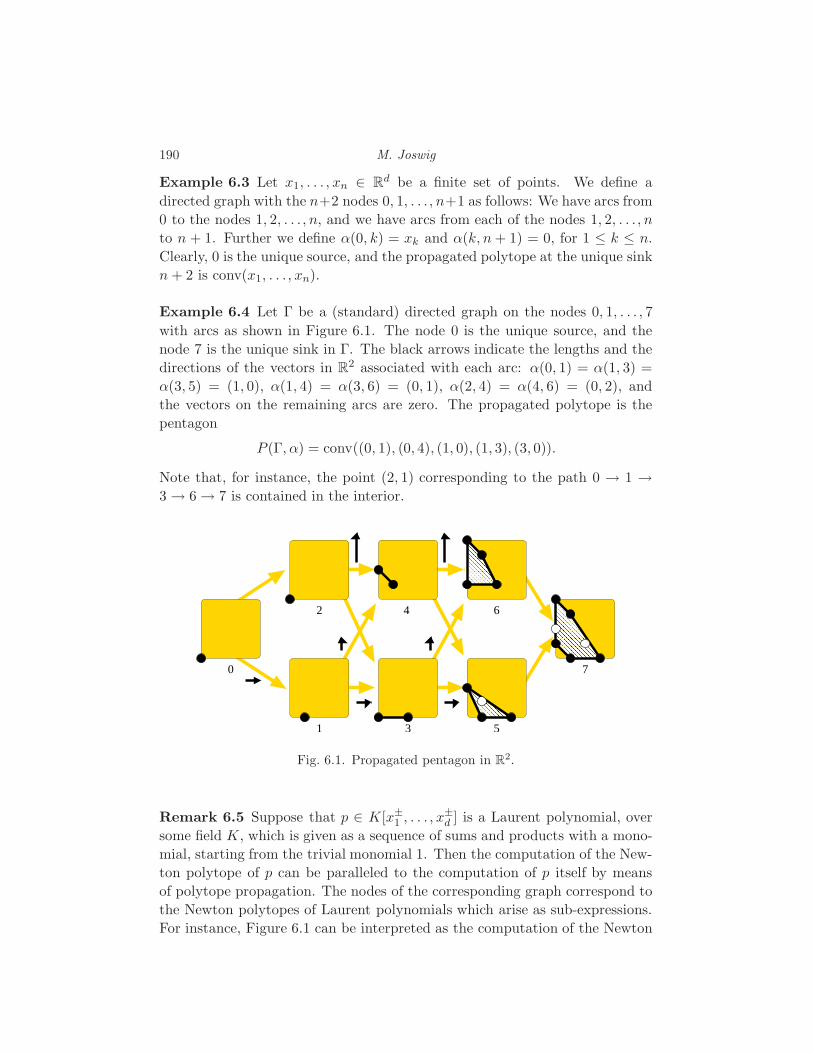
190 M. Joswig
Example 6.3 Let x1, . . . , xn ∈ Rd be a finite set of points. We define a
directed graph with the n+2 nodes 0, 1, . . . , n+1 as follows: We have arcs from
0 to the nodes 1, 2, . . . , n, and we have arcs from each of the nodes 1, 2, . . . , n
to n + 1. Further we define α(0, k) = xk and α(k, n+ 1) = 0, for 1 ≤ k ≤ n.
Clearly, 0 is the unique source, and the propagated polytope at the unique sink
n + 2 is conv(x1, . . . , xn).
Example 6.4 Let Γ be a (standard) directed graph on the nodes 0, 1, . . . , 7
with arcs as shown in Figure 6.1. The node 0 is the unique source, and the
node 7 is the unique sink in Γ. The black arrows indicate the lengths and the
directions of the vectors in R2 associated with each arc: α(0, 1) = α(1, 3) =
α(3, 5) = (1, 0), α(1, 4) = α(3, 6) = (0, 1), α(2, 4) = α(4, 6) = (0, 2), and
the vectors on the remaining arcs are zero. The propagated polytope is the
pentagon
P (Γ, α) = conv((0, 1), (0, 4), (1, 0), (1, 3), (3, 0)).
Note that, for instance, the point (2, 1) corresponding to the path 0 → 1 →3 → 6 → 7 is contained in the interior.
0
2
1
4
3 5
6
7
Fig. 6.1. Propagated pentagon in R2.
Remark 6.5 Suppose that p ∈ K[x±1 , . . . , x±d ] is a Laurent polynomial, over
some field K, which is given as a sequence of sums and products with a mono-
mial, starting from the trivial monomial 1. Then the computation of the New-
ton polytope of p can be paralleled to the computation of p itself by means
of polytope propagation. The nodes of the corresponding graph correspond to
the Newton polytopes of Laurent polynomials which arise as sub-expressions.
For instance, Figure 6.1 can be interpreted as the computation of the Newton

Polytope Propagation on Graphs 191
polytope of p = x + x3 + xy + xy3 + x2y + y + y2 + y4. Denoting by p(i)
the polynomial associated with node i, we have p(0) = p(2) = 1, p(2) = x,
p(3) = 1+x2, p(4) = xy+y2, p(5) = x+x3 +xy+y2 , p(6) = x2y+xy3 +y+y4 ,
and p(7) = p. Note that, since we keep adding polynomials with non-negative
coefficients, cancellation does not occur.
Example 6.6 A zonotope Z is the Minkowski sum of k line segments [pi, qi] ⊂Rd or, equivalently, an affine projection of the regular k-cube. Each zonotope
can be obtained by polytope propagation as follows: Take the vertex edge
graph Γk of the regular cube [0, 1]k and direct its edges according to the linear
objective function∑xi. Let α(x, x + ei) = qi − pi for each arc (x, x + ei),
where x and x+ ei are neighboring vertices of [0, 1]k. Like in Example 6.1 the
propagated polytope at each node of Γk is a point. Now construct a (standard)
directed graph Γ∗k from Γk by adding one additional node ∞ and arcs, with
the zero vector associated, from each node of Γk to ∞. Up to a translation by
the vector∑pi the propagated polytope at ∞ is the zonotope Z. Figure 6.2
shows the construction of a centrally symmetric hexagon.
Fig. 6.2. Zonotope with three zones (here corresponding to the three parallel classesof solid arcs) in R2 as propagated polytope. The arcs of the graph Γ∗
3 which are notarcs of Γ3 are dashed; see Example 6.6.
Theorem 6.7 Let Γ be a standard directed acyclic graph. Then the vertices
of the polytope propagated by Γ can be computed in time which is polynomially
bounded in the size of Γ.
192 M. Joswig
Proof Let s be the unique sink of Γ. By induction we can assume that the
vertices of the polytopes propagated to the nodes which have an arc to s can
be computed in polynomial time. In particular, their total number is bounded
by a polynomial in the size of Γ.
If P = convx1, . . . , xn is a polytope in Rd then a point xk is a vertex
if and only if it can be separated from x1, . . . , xk−1, xk+1, . . . , xn by an affine
hyperplane. The linear optimization problem:
maximize ǫ subject to
λ0, . . . , λd ∈ R, ǫ ≥ 0,
d∑
j=1
λjxij ≤ λ0 − ǫ, for each i 6= k,
d∑
j=1
λjxkj ≥ λ0 + ǫ
(6.1)
has a solution with ǫ > 0 if and only if xi is a vertex of P . Since linear optimiza-
tion is solvable in polynomial time, see [Hacijan, 1979, Grotschel et al., 1993],
the claim follows.
The above rough estimation of the complexity of polytope propagation is
slightly incomplete. The linear optimization problem 6.1 can be solved in O(n)
time if d is fixed, see [Megiddo, 1984], and hence finding all the vertices of P =
convx1, . . . , xn takes O(n2) time in fixed dimension. Moreover, computing
convex hulls in R2 or R3 only takes at most O(n logn) time, see [Seidel, 2004].
Hence computing convex hulls directly is superior to the approach described
above, for the special case of d ≤ 3.
6.3 Specialization to Hidden Markov Models
We consider a finite Markov process with l states and transition matrix θ′ =
(θ′ij) ∈ Rl×l satisfying the conditions θ′ij ≥ 0 and∑
j θ′ij = 1. The value
θ′ij is the transition probability of going from state i into state j. In the
hidden Markov model we additionally take into account that the observation
itself may be a probabilistic function of the state. That is to say, there are l′
possible observations (where l′ may even be different from l) and a non-negative
matrix θ′′ = (θ′′ij) ∈ Rl×l′ satisfying∑
j θ′′ij = 1. The entry θ′′ij expresses the
probability that j has been observed provided that the actual state was i. In
the following we will be concerned with parameterized hidden Markov models
as in Chapter 1.
Example 6.8 The simplest possible (non-trivial) HMM occurs for l = l′ = 2
Polytope Propagation on Graphs 193
and θ′ =(
θ′00 θ′01θ′10 θ′11
), θ′′ =
(θ′′00 θ′′01θ′′10 θ′′11
). If, for instance, we observe our primary
process for three steps, the sequence of observations is some bit-string β0β1β2 ∈0, 13. There are eight possible sequences of states which may have led to this
observation. As in Chapter 1 we assume that the initial state of the primary
process attains both states with equal probability 12 . Then we have that
Prob[Y0 = β0, Y1 = β1, Y2 = β2] =1
2
∑
σ∈0,13
θ′σ0σ1θ′σ1σ2
θ′′σ0β0θ′′σ1β1
θ′′σ2β2.
Now let us have a look at the parameterized model, where —for the sake of
simplicity— we assume that θ′ = θ′′ = ( u vv w ) is symmetric. Since otherwise
our primary process would be stationary, we can additionally assume v 6= 0.
Neglecting the probabilistic constraints and re-scaling then allows to study the
parameterized HMM of
η′ = η′′ =
(x 1
1 y
)∈ R[x, y]2×2.
The probability to make the specific observation 011 in the parameterized
model yields
Prob[Y0 = 0, Y1 = 1, Y2 = 1] =1
2(x3 + x2y + xy + xy3 + x+ y + y2 + y4),
which happens to be the polynomial p in Remark 6.5 (up to the constant factor12 ), and whose Newton polytope is the pentagon in Figure 6.1.
The fixed observation β1 · · ·βn of a hidden Markov model θ = (θ′, θ′′) for
n steps gives rise to the standardized acyclic directed graph Γnθ with node set
[n]×[l]∪−∞,+∞ as follows: There is an arc from −∞ to all nodes (1, j), and
there is an arc from (n, j) to +∞ for all j ∈ [l]; further, there is an arc between
(i, j) and (i+ 1, k) for any i, j, k. The directed paths from the unique source
−∞ to the unique sink +∞ directly correspond to the ln possible sequences
of states of the primary process that may or may not have led to the given
observation β1 · · ·βn. Such a path passes through the node (i, j) if and only if
the i-th primary state Xi has been j.
The probability thatXi−1 = j andXi = k under the condition that Yi = βi is
the monomial θ′jkθ′′k,βi
∈ R[θ′11, . . . , θ′ll, θ′′11, . . . , θ
′′ll′]. We associate its (integral)
exponent vector with the arc (i − 1, j) → (i, k). Likewise, we associate the
exponent vector of θ′′k,β0with the arc −∞ → (0, k) and 0 to all arcs (l−1, k) →
+∞.
The graph Γnθ gives rise to a propagated polytope whose vertices correspond
to most likely explanations for the observation made for some choice of param-
eters.
194 M. Joswig
This schema can be modified by specializing some of the parameters as in
Example 6.8. The associated graph is given as Example 6.4, and its propagated
polytope is the Newton polytope of the polynomial p(7) in Remark 6.5, a
pentagon.
In our scheme of polytope propagation we chose to restrict the information
on the arcs to be single points (which are 0-dimensional polytopes). For this
reason we chose our parametric HMM to have monomials for the transition
probabilities. It is conceivable (but not implemented in polymake) to allow for
arbitrary polynomials for the transition probabilities. This would then require
to iteratively compute Minkowski sums of higher dimensional polytopes. For
Minkowski sum algorithms for general polytopes see [Fukuda, 2004].
6.4 An Implementation in polymake
We give a complete listing of the program sum_product, which implements
the algorithm described. In order to increase the legibility the code has been
re-arranged and shortened slightly.
6.4.1 Main Program and the polymake Template Library
The main program sets up the communication with the polymake server for
the polytope object p, which is contains the propagation graph Γ and the
function α. The graph Γ is assumed to be standard, and the polytope object
p corresponds to the propagated polytope P (Γ, α). The class Poly is derived
from iostream. The actual function which does the job is sum_product in the
namespace polymake::polytope.
using namespace polymake;
int main(int argc, char *argv[]) if (argc != 2)
cerr << "usage: " << argv[0] << " <file>" << endl;return 1;
try
Poly p(argv[1], ios::in | ios::out);polytope::sum_product(p);
catch (const std::exception& e)
cerr << e.what() << endl;return 1;
return 0;

Polytope Propagation on Graphs 195
The polymake system comprises a rich template library which complies with
the Standard Template Library (STL). This includes a variety of container
template classes, such as Array (which is a variation of STL’s vector class)
and template classes for doing linear algebra, such as Vector and Matrix.
Additionally, there are several classes which special functionality useful in al-
gorithmic polytope theory, for example, Graph and IncidenceMatrix.
A common feature of polymake’s container classes is a memory management
based on reference counting (with copy-on-write). Hence copying a non-altered
Array, for example, costs next to nothing. Further all these classes provide a
range of features useful for debugging. The reader is referred to the polymake’s
documentation for a detailed description.
The arithmetic operations use exact representations of rational numbers.
Our class Rational wraps the corresponding implementation from the GNU
Multiprecision Library.
The rest of this section lists the function sum_product in the namespace
polymake::polytope.
namespace polymake namespace polytope ...
6.4.2 The core of the implementation
The graph that the client reads already comes with a (translation) vector
specified for each edge. This is the second template parameter. The first
template parameter is set to an artificial type nothing which means that do
not have any data at the nodes The third template parameter (again some
artificial type) indicates that our graph is directed. We assume that the graph
is acyclic with a unique sink. Arbitrarily many sources are allowed.
typedef Graph< nothing, Vector<Rational>, directed > graph;
We now start to describe the actual polytope propagation algorithm. It
operates on a single Poly object from which the SUM_PRODUCT_GRAPH is read.
It writes the VERTICES and VERTEX_NORMALS of the polytope corresponding to
the unique sink in the graph.
void sum_product(Poly& p) ...
Read the graph and the dimension of the ambient space. The member func-
tion give() of the Poly class induces the polymake server to deliver the named
property of the object p; if necessary the server triggers further computations,
as defined by an extensible set of rules, to answer the request made. There is
a reciprocal function take() to be used further below.
const graph G=p.give("SUM_PRODUCT_GRAPH");const int n(G.nodes());

196 M. Joswig
if (n==0)throw std::runtime_error("SUM_PRODUCT_GRAPH must be non-empty");
const int d=p.give("AMBIENT_DIM");
Below is given the description of the origin as a 0-dimensional polytope
(living in d-space). It has one vertex and en empty vertex-facet incidence
matrix. This is used to define the initial objects of type Poly for the sources
of the graph.
const Matrix<Rational> single_point_vertices(vector2row(unit_vector<Rational>(d+1,0)));
const IncidenceMatrix<> single_point_vif;
The following defines an array where all the intermediate polytopes are
stored. The nodes in the graph are consecutively numbered, starting with
0. The corresponding polytope can be accessed by indexing the array pa with
the node number. In the beginning the Poly objects are undefined.
Array<Poly> pa(n);std::list<int> next_nodes;
Initialize by assigning a single point (origin) to each source in the graph.
for (int v=0; v<n; ++v) if (G.in_degree(v)==0)
pa[v].init(0, ios::in | ios::out | ios::trunc,"RationalPolytope");
pa[v].take("VERTICES") << single_point_vertices;pa[v].take("VERTICES_IN_FACETS") << single_point_vif;add_next_generation(next_nodes,v,G,pa);
At each node of the graph recursively define a polytope as the convex hullof the translated predecessors. We also try to find the sink on the way.
int sink=-1;
The number −1 does not correspond to any valid node number; it indicates
that no sink has been found yet.
while(!next_nodes.empty())
Get some node w for which we already know all its predecessors. Initialize
the client-server communication for that node’s polytope. Until now it was
undefined.
const int w=next_nodes.front(); next_nodes.pop_front();pa[w].init(0, ios::in | ios::out, "RationalPolytope");

Polytope Propagation on Graphs 197
The polytope will be specified as the convex hull of points, which will be
collected from other polytopes. The special data type ListMatrix is efficient in
terms of concatenating rows (which correspond to points) but it is not efficient
in terms of matrix operations (although all operations are defined). This is
acceptable, since we do not compute anything in this step. The C++ operator
/ takes care of the concatenation of compatible matrix blocks on top of one
another.
ListMatrix< Vector<Rational> > points(0,d+1);for (Entire<graph::in_edge_list>::const_iterator
e=entire(G.in_edges(w)); !e.at_end(); ++e)
The node v is the current predecessor to process. The arc from v to w is e.
The operator * extracts the associated vector from an arc.
const int v=e.from_node();const Vector<Rational> vec=*e;
Next we read the vertices of the predecessor polytope. polymake’s rule
basis by default uses cdd’s implementation to check for redundant (= non-
vertex) points among the input by solving linear programs. No convex hull
computation is necessary. What is going on behind the scene is hidden from
the user. The polymake server decides how to produce the VERTICES of the
polytope object pa[v]. Note that this is the same behavior as if polymake
would asked for these vertices via the command line interface.
const Matrix<Rational> these_vertices=pa[v].give("VERTICES");
Now concatenate the translated matrix (where the rows correspond to the
vertices of the predecessor) to what we already have. The final closes the
for-loop through all the predecessors of w.
points /= these_vertices*translation_by(vec);
Define the polytope object as the convex hull of all those points collected
and proceed.
pa[w].take("POINTS") << points;if (G.out_degree(w)==0) sink=w;else add_next_generation(next_nodes,w,G,pa);
This will be just any sink; it is indeterministic if the graph does have several
sinks.
if (sink<0)throw std::runtime_error("no sink found in digraph");

198 M. Joswig
The sink defines the polytope we are after and this is going to be defined
as the polytope object p. The vertex normals serve as certificates that the
claimed points are indeed vertices.
const Matrix<Rational>sink_vertices = pa[sink].give("VERTICES"),sink_normals = pa[sink].give("VERTEX_NORMALS");
p.take("VERTICES") << sink_vertices;p.take("VERTEX_NORMALS") << sink_normals;
6.4.3 Two auxiliary functions
The first one gathers the next generation of graph nodes which can be defined
at that stage, since all predecessors known. It is one step in a common breadth
first search. The graph nodes which can be processed (because all their pre-
decessors are known) are stored in a doubly linked list, that is STL’s type
list.
void add_next_generation(std::list<int>& next_nodes, const int v,const graph& G, const Array<Poly>& pa)
for (Entire<graph::out_edge_list>::const_iterator
e=entire(G.out_edges(v)); !e.at_end(); ++e) const int x=e.to_node();Entire<graph::in_edge_list>::const_iterator
f=entire(G.in_edges(x));for( ; !f.at_end() && pa[f.from_node()].get_mode(); ++f);if (f.at_end())
next_nodes.push_back(x);
The following function returns a translation matrix (to be applied to row
vectors from the right) for given vector. The C++ operators | and / are
overloaded for the Matrix class: They define the concatenation of two matrix
blocks side by side and one on top of the other, respectively.
Matrix<Rational> translation_by(const Vector<Rational>& vec)
const int d=vec.dim();return unit_vector<Rational>(d+1,0) |
(vec / unit_matrix<Rational>(d));

Polytope Propagation on Graphs 199
6.5 Returning to Our Example
There is another standard client program binary-markov-graph which pro-
duces the polytope propagation graphs for the special HMM discussed in Ex-
ample 6.8. It can be called from the command line as follows:
> binary-markov-graph b011.poly 011
Here the argument 011 specifies the observation. The command yields a file
b011.poly which contains a description of the polytope propagation suitable
as input for the sum_product client.
> sum_product b011.poly
This defines a polytope object, which is accessible to all of polymake’s func-
tions. For example, this is how to list all the vertices of the propagated poly-
tope. Each row corresponds to a vertex of our pentagon (first column used for
homogenization of the coordinates).
> polymake b011.poly VERTICES
VERTICES
1 3 0
1 1 0
1 0 1
1 1 3
1 0 4

7
Parametric Sequence Alignment
Colin Dewey
Kevin Woods
The alignment of DNA and protein sequences is one of the most fundamen-
tal problems in computational biology. Section 2.2 introduced some scoring
schemes and algorithms used for global alignment of two biological sequences.
Each scoring scheme is dependent on a set of parameters, and, as Example 2.14
showed, the optimal alignment can change significantly as these parameters
are varied. Users of alignment algorithms would like to know how their results
are affected by the values of the parameters and how confident they can be
in a given optimal alignment. Such questions are answered using parametric
sequence alignment methods. In this chapter, the techniques of parametric
sequence alignment are introduced and later applied to characterize a couple
of simple scoring schemes. As parametric alignment algorithms can be im-
plemented almost as efficiently as algorithms for normal sequence alignment,
parametric sequence alignment methods are powerful and important compo-
nents of the computational biologist’s toolbox.
7.1 Few alignments are optimal
The primary goal of biological sequence alignment is to match up positions in
the input sequences that are homologous. Two sequence positions are homol-
ogous if the characters at those positions are derived from the same position
in some ancestral sequence. It is important to note that two positions can be
homologous even though the states of the positions are different. For example,
position 5 in σ1 and position 9 in σ2 may be homologous despite the fact that
σ15 = A and σ2
9 = C. Alignments indicate that positions in two sequences are
homologous by matching up the characters at those positions. An alignment
is biologically correct if it matches up all positions that are truly homologous
and no others. Because this chapter focuses on the global alignment problem
for two sequences, we will ignore cases in which a duplication event causes one
position to be homologous to multiple positions in the other sequence.
200
Parametric Sequence Alignment 201
What does it mean for a global alignment to be “optimal”? If our goal is to
discover the biological truth, we should say that an “optimal” global alignment
is one that is biologically correct. Having biologically correct alignments is
critical because other analyses, such as phylogenetic tree construction, are
heavily dependent on sequence alignments. Unfortunately, in most cases, we
do not know what the biological truth is. We must therefore use a scoring
scheme to rank the alignments and take the highest-ranking alignment as our
best guess of the truth. Which scoring scheme should we use to make such a
guess? Once we have chosen our parameter values, how confident can we be
that the resulting alignment is a good guess? It could be the case that, if we
vary our chosen parameter values just slightly, we will obtain very different
alignments. Even worse, it could be that no values for the parameters of our
chosen scoring scheme will give the biologically correct alignment as being
optimal.
The methods of parametric sequence alignment help to answer these ques-
tions, for specific input sequences, by analyzing a scoring scheme over all pos-
sible parameter values. Specifically, parametric sequence alignment subdivides
the parameter space into regions such that parameter values in the same region
give rise to the same optimal alignments. Such a subdivision tells us which of
the exponentially-many possible alignments can be optimal for some choice of
parameter values and how many classes of optimal alignments there can be.
In addition, if we find that the point in the parameter space corresponding
to our current choice of values for the parameters is close to the boundary of
a region in the subdivision, we may be less confident in our results. This is
because varying the parameter values slightly is likely to move the point to
a different region in the subdivision and thus produce different optimal align-
ments. Lastly, we may wish to take a Bayesian approach and place a prior
distribution on the parameters. In this case, we can determine what the most
likely optimal alignments are by integrating over the different regions in the
subdivision (note that this is different from finding the most likely alignment)
[Pachter and Sturmfels, 2004b].
Parametric sequence alignment is feasible, because, although two given se-
quences have exponentially-many possible alignments, there are only a few
subsets of these alignments (corresponding to regions of the parameter space
subdivision) that can be optimal for some choice of parameters. For two se-
quences of length at most n, it has been shown that for a simple scoring scheme
with 2 parameters allowed to vary, the number of regions in the subdivision is
O(n23 ) [Gusfield et al., 1994]. This bound corresponds exactly with the bound
given in Section 5.3 for the number of vertices of a sequence alignment Newton
polytope with d = 2. In fact, for a scoring scheme with any number of param-
eters, the number of regions is bounded by a polynomial in n (see Section 5.3).

202 C. Dewey and K. Woods
The bound on the number of regions in the subdivision allows for the subdivi-
sion to be determined in just slightly more time than it takes to simply align
the sequences in question. For the simple scoring scheme just mentioned, the
subdivision can be found in O(n83 ) time, as opposed to O(n2) time for aligning
the sequences with a fixed set of parameter values.
The concept of parametric sequence alignment is not a new one, and there
are several programs available to perform parametric analysis [Gusfield, 1997].
Existing methods are restricted to the analysis of scoring schemes with at
most 2 parameters allowed to vary at one time, whereas we may also like to
analyze scoring schemes that have many parameters, such as the general 33-
parameter scoring scheme described in Section 2.2. In this chapter, we apply
the techniques of parametric inference described in Chapter 5 to the problem
of sequence alignment and thus give a general method for parametric sequence
analysis with scoring schemes involving any number of parameters.
7.2 Polytope propagation for alignments
In this section, we will describe how to efficiently compute a parametric se-
quence alignment of two sequences, σ1 and σ2, with lengths n and m, re-
spectively. While the method we describe can be used to analyze a fully-
parameterized scoring scheme (with the 33 parameters comprising the matrices
shown in Equations 2.11 and 2.12), we will concentrate on a simple 4-parameter
scoring scheme, with parametersM , X , S, andG, corresponding to the weights
for matches, mismatches, spaces (- symbols in the alignment), and gaps (con-
tiguous sets of spaces), respectively. This scoring scheme is just a special case
of the general scoring scheme with
wπ,π = M ∀π ∈ Σ
wπ1,π2 = X ∀π1, π2 ∈ Σ, π1 6= π2
wπ,− = w−,π = S ∀π ∈ Σ
w′H,I = w′H,D = w′I,D = w′D,I = G
w′H,H = w′I,H = w′D,H = w′I,I = w′D,D = 0 .
An even simpler scoring scheme, which we will refer to as the 3-parameter scor-
ing scheme, has G = 0. We shall present a method for parametric alignment
with the 3-parameter scoring scheme, but it should be noted that this method
easily generalizes to the 4-parameter and 33-parameter scoring schemes.
With the 3-parameter scoring scheme, the weight of an alignment, h, is
Wσ1,σ2(h) = Mmh +Xxh + Ssh, (7.1)
where mh, xh, and sh denote the number of matches, mismatches, and spaces
Parametric Sequence Alignment 203
in h, respectively. We define the monomial
fσ1,σ2,h = θmhM θxh
X θshS (7.2)
and the polynomial
fσ1,σ2 =∑
h∈An,m
fσ1,σ2,h. (7.3)
The weight, W (h), is simply log fσ1,σ2,h(eM , eX , eS). As we saw in Section 2.2,
finding the alignment, h, that minimizesW (h) is equivalent to evaluating fσ1,σ2
tropically. Following with tradition, we will choose to maximize W (h) in this
chapter, but these are equivalent problems.
The parametric alignment problem for this scoring scheme, then, is to com-
pute which values of M , X , and S result in which optimal alignments. The
key object in our parametric alignment of σ1 and σ2 is the Newton polytope
of the polynomial fσ1,σ2. The Newton polytope of fσ1,σ2 is the convex hull of
all points (mh, xh, sh), for h ∈ An,m. Recall from Section 2.3 that each vertex
of NP(fσ1,σ2) corresponds to an alignment (or set of alignments, all having the
same number of matches, mismatches, and spaces) that will be optimal for a
certain set of values for the parameters, M , X , and S. For a vertex, v, of
NP(fσ1,σ2), the set of parameters for which the alignments corresponding to v
are all optimal is given by its normal cone N (v). The normal fan of the Newton
polytope, N (NP(fσ1,σ2)) is thus a subdivision of the parameter space with the
property that, for all parameter values in the same region (normal cone), the
same alignments are optimal. This subdivision is exactly the desired output
of parametric sequence alignment.
Having shown that the Newton polytope of fσ1,σ2 and its corresponding
normal fan solve the parametric alignment problem, we now turn to how to
compute these objects efficiently using the polytope propagation algorithm of
Chapter 5. First, however, we make two remarks that will make our presenta-
tion cleaner.
Remark 7.1 For an alignment, h, of σ1 and σ2, we must have that 2mh +
2xh + sh = n +m.
Proof Recall from Section 2.2 that h is a string over the alphabet H, I, D.Matches and mismatches correspond to H characters in the alignment, while
spaces correspond to I and D characters. The remark follows from combining
the equalities in Equation 2.7.
Remark 7.2 Any 3-parameter scoring scheme (M,X, S) is equivalent to an-
other scoring scheme (M ′, X ′, S ′), whereM ′ = 0, X ′ = X−M , and S ′ = S−M2 .
204 C. Dewey and K. Woods
Proof Using Remark 7.1, we have that
W ′(h) = M ′mh +X ′xh + S ′sh = W (h) − M
2(n+m) = W (h) −C,
where C = M2 (n+m) is a constant with respect to the alignment h. Since all
scores are shifted by the same constant, the rankings of possible alignments
under the two scoring schemes are the same.
Having made this remark, we now assume that M = 0 for the remainder of
this section. With this specialization (and setting θM = eM = 1), we have
fσ1,σ2 =∑
h∈An,m
θxhX θsh
S ,
and our Newton polytope and normal fan will be two-dimensional.
Let us briefly recall the Needleman-Wunsch algorithm, which, given specific
parameter values X and S and sequences σ1 and σ2, computes the optimal
global alignment. Let σ1 = σ11σ
12 · · ·σ1
n and σ2 = σ21σ
22 · · ·σ2
m. For 0 ≤ i ≤ n,
define
σ1≤i = σ1
1σ12 · · ·σ1
i ,
and similarly define σ2≤j to be the first j characters in σ2. Define M [i, j] to
be the score of the optimal alignment of σ1≤i and σ2
≤j . We would like to find
M [n,m], and we do this recursively as follows. For characters π1 and π2 in
Σ, define w(π1, π2) to be 0 if π1 = π2 and X if π1 6= π2. For the base cases
of the recursion, we have that M [i, 0] = i · S and M [0, j] = j · S (since the
only alignments have i spaces and j spaces, respectively). Then we recursively
apply the formula
M [i, j] = max
M [i− 1, j − 1] +w(σ1i , σ
2j )
M [i− 1, j] + S
M [i, j − 1] + S
(7.4)
for 1 ≤ i ≤ n and 1 ≤ j ≤m.
Example 7.3 Suppose that σ1 = CAA and σ2 = AAC, and we have parameter
values M = 0, X = −2, and S = −3. Then Figure 7.1 shows M [i, j] for
0 ≤ i, j ≤ 3. In particular, the optimal alignment for σ1 and σ2 is CAAAAC with
score M [3, 3] = −4.
In the recursive formula for the Needleman-Wunsch algorithm, we use two
operations, max and +. In other words, the recursion takes place in the
(max,+) algebra (which is equivalent to the tropical algebra). The polytope
propagation algorithm is the exact same recursion, but in the polytope algebra
(Section 2.3), where addition is the convex hull of the union of two polytopes
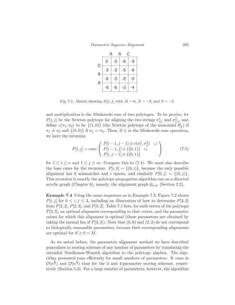
Parametric Sequence Alignment 205
A C
C
A
A
A
0 -3 -9-6
-3
-6
-9
-2
-3
-5 -6
-2 -5
-6 -3 -4
Fig. 7.1. Matrix showing M [i, j] with M = 0, X = −2, and S = −3.
and multiplication is the Minkowski sum of two polytopes. To be precise, let
P [i, j] be the Newton polytope for aligning the two strings σ1≤i and σ2
≤j , and
define v(π1, π2) to be (1, 0) (the Newton polytope of the monomial θ1X) if
π1 6= π2 and (0, 0) if π1 = π2. Then, if ⊕ is the Minkowski sum operation,
we have the recursion
P [i, j] = conv
P [i− 1, j − 1] ⊕ v(σ1i , σ
2j ) ∪
P [i− 1, j]⊕ (0, 1) ∪P [i, j − 1]⊕ (0, 1)
(7.5)
for 1 ≤ i ≤ n and 1 ≤ j ≤ m. Compare this to (7.4). We must also describe
the base cases for the recursion: P [i, 0] = (0, i), because the only possible
alignment has 0 mismatches and i spaces, and similarly P [0, j] = (0, j).This recursion is exactly the polytope propagation algorithm run on a directed
acyclic graph (Chapter 6), namely, the alignment graph Gn,m (Section 2.2).
Example 7.4 Using the same sequences as in Example 7.3, Figure 7.2 shows
P [i, j] for 0 ≤ i, j ≤ 3, including an illustration of how to determine P [3, 3]
from P [2, 2], P [2, 3], and P [3, 2]. Table 7.1 lists, for each vertex of the polytope
P [3, 3], an optimal alignment corresponding to that vertex, and the parameter
values for which this alignment is optimal (these parameters are obtained by
taking the normal fan of P [3, 3]). Note that (0, 6) and (2, 2) do not correspond
to biologically reasonable parameters, because their corresponding alignments
are optimal for S ≥ 0 = M .
As we noted before, the parametric alignment method we have described
generalizes to scoring schemes of any number of parameters by translating the
extended Needleman-Wunsch algorithm to the polytope algebra. The algo-
rithm presented runs efficiently for small numbers of parameters. It runs in
O(n83 ) and O(n
72 ) time for the 3 and 4-parameter scoring schemes, respec-
tively (Section 5.3). For a large number of parameters, however, the algorithm
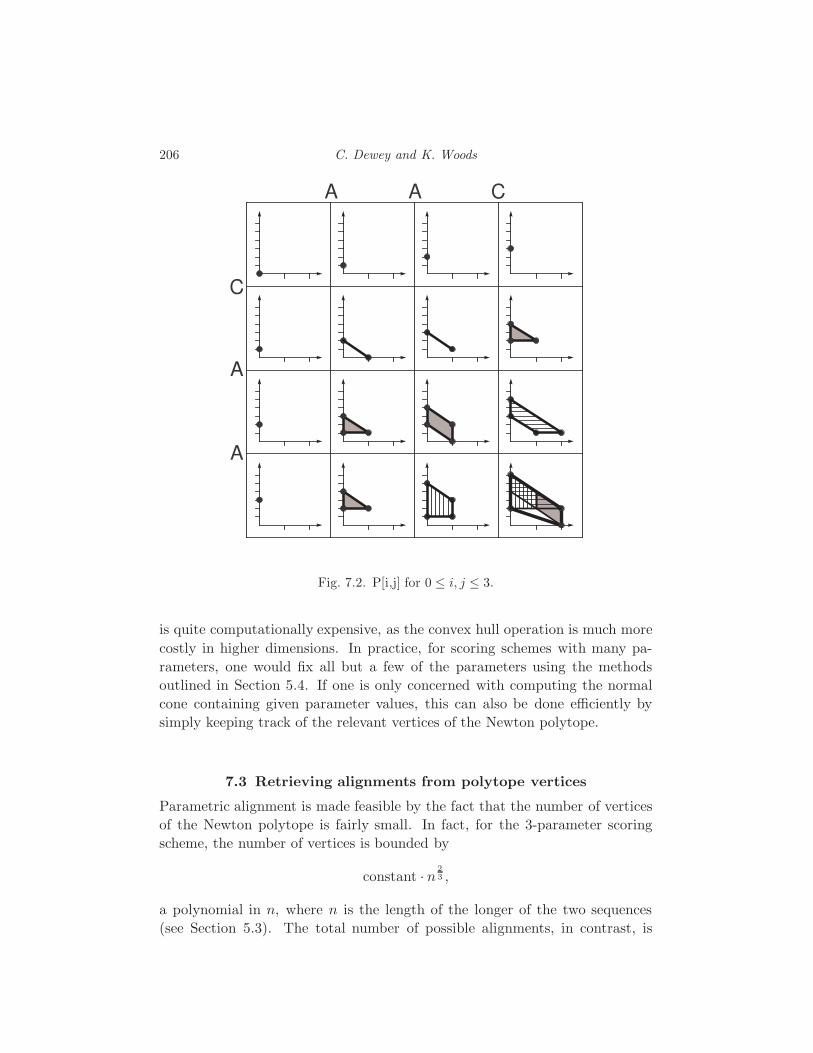
206 C. Dewey and K. Woods
A C
C
A
A
A
Fig. 7.2. P[i,j] for 0 ≤ i, j ≤ 3.
is quite computationally expensive, as the convex hull operation is much more
costly in higher dimensions. In practice, for scoring schemes with many pa-
rameters, one would fix all but a few of the parameters using the methods
outlined in Section 5.4. If one is only concerned with computing the normal
cone containing given parameter values, this can also be done efficiently by
simply keeping track of the relevant vertices of the Newton polytope.
7.3 Retrieving alignments from polytope vertices
Parametric alignment is made feasible by the fact that the number of vertices
of the Newton polytope is fairly small. In fact, for the 3-parameter scoring
scheme, the number of vertices is bounded by
constant · n 23 ,
a polynomial in n, where n is the length of the longer of the two sequences
(see Section 5.3). The total number of possible alignments, in contrast, is
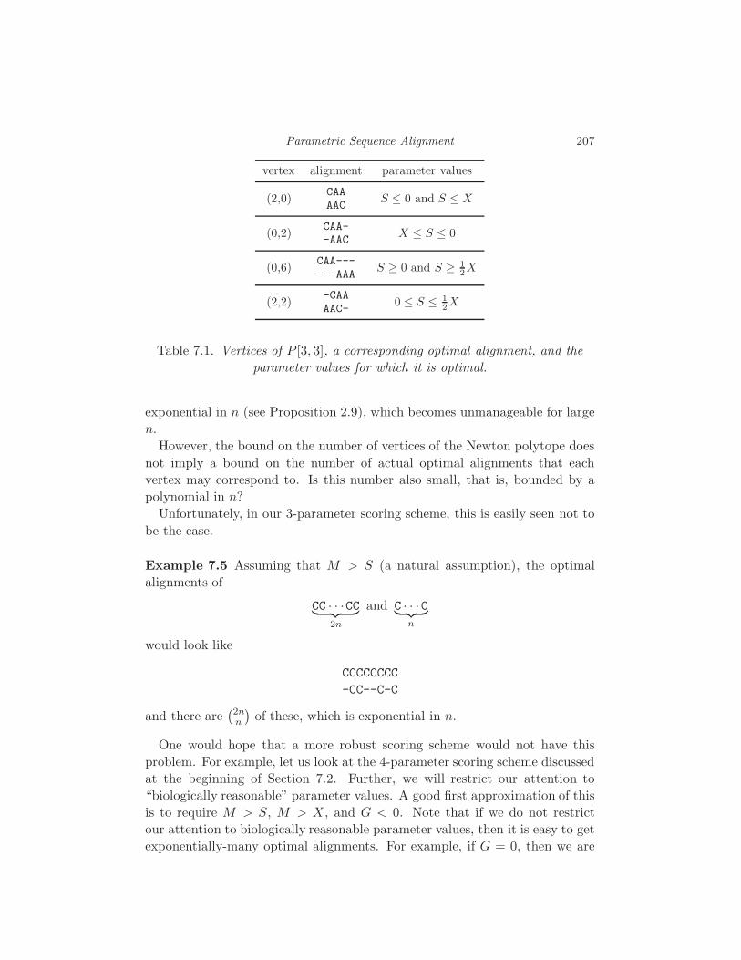
Parametric Sequence Alignment 207
vertex alignment parameter values
(2,0)CAAAAC
S ≤ 0 and S ≤ X
(0,2)CAA--AAC
X ≤ S ≤ 0
(0,6)CAA------AAA
S ≥ 0 and S ≥ 12X
(2,2)-CAAAAC-
0 ≤ S ≤ 12X
Table 7.1. Vertices of P [3, 3], a corresponding optimal alignment, and the
parameter values for which it is optimal.
exponential in n (see Proposition 2.9), which becomes unmanageable for large
n.
However, the bound on the number of vertices of the Newton polytope does
not imply a bound on the number of actual optimal alignments that each
vertex may correspond to. Is this number also small, that is, bounded by a
polynomial in n?
Unfortunately, in our 3-parameter scoring scheme, this is easily seen not to
be the case.
Example 7.5 Assuming that M > S (a natural assumption), the optimal
alignments of
CC · · ·CC︸ ︷︷ ︸2n
and C · · ·C︸ ︷︷ ︸n
would look like
CCCCCCCC
-CC--C-C
and there are(2n
n
)of these, which is exponential in n.
One would hope that a more robust scoring scheme would not have this
problem. For example, let us look at the 4-parameter scoring scheme discussed
at the beginning of Section 7.2. Further, we will restrict our attention to
“biologically reasonable” parameter values. A good first approximation of this
is to require M > S, M > X , and G < 0. Note that if we do not restrict
our attention to biologically reasonable parameter values, then it is easy to get
exponentially-many optimal alignments. For example, if G = 0, then we are

208 C. Dewey and K. Woods
reduced to the 3-parameter scoring scheme, and Example 7.5 shows sequences
with(2n
n
)optimal alignments.
Small experiments do lead one to believe that, if the parameters are biologi-
cally reasonable, then there are not “too many” optimal alignments. Unfortu-
nately, for each such choice of parameters, there are sequences with exponen-
tially many optimal alignments.
Proposition 7.6 Given parameters M,X,G, and S such that M > X , M >
S, and G < 0, choose any k ∈ Z+ such that
k >−G
M − maxX, S.
For a given m ∈ Z+, define the sequences σ1 and σ2 of lengths 4km and 3km,
respectively, as follows: σ1 is
AA · · ·AA︸ ︷︷ ︸2k
CC · · ·CC︸ ︷︷ ︸2k
repeated m times, and σ2 is
AA · · ·AA︸ ︷︷ ︸2k
C · · ·C︸ ︷︷ ︸k
also repeated m times.
Then there are exactly (k+ 1)m optimal alignments, which is exponential in
the lengths of σ1 and σ2.
Proof The obvious choice for optimal alignments are ones like
AAAACCCCAAAACCCCAAAACCCC
AAAACC--AAAAC--CAAAA--CC
(in this example, k = 2 and m = 3) with all of the A’s aligned and with one
gap in each block of C’s in σ2. Since there are m blocks of C’s and k+1 choices
of where to place the gap in each block, there are (k+1)m of these alignments.
Let O denote the set of such alignments. We must prove that there are no
alignments better than those in O.
Note that these alignments have the greatest possible number of matches
(3km) and the least possible number of mismatches (zero). Therefore, the
only way to improve the alignment is to have fewer gaps. Suppose we have
a new alignment, h, with a better score than those in O. We will divide the
alignment scores into 2 parts:
(i) score from gaps in σ2, and
(ii) score from gaps in σ1, and from matches and mismatches in the align-
ment.

Parametric Sequence Alignment 209
Let n be the number of gaps in h appearing in σ2 (there may also be gaps
in σ1). Then n < m, because having fewer gaps is the only way to improve on
the score of the alignments in O. Part 1 of the score is increased by at most
(m− n)(−G),
since the alignments in O have m gaps and km spaces, and h has n gaps and
at least km spaces in σ2.
To see how much part 2 of the score is decreased by changing from an
alignment in O to the alignment h, we partition σ2 into m+ 1 blocks
A · · ·A︸ ︷︷ ︸k
∣∣∣
m−1︷ ︸︸ ︷A · · ·A︸ ︷︷ ︸
k
C · · ·C︸ ︷︷ ︸k
A · · ·A︸ ︷︷ ︸k
∣∣∣ · · ·∣∣∣ A · · ·A︸ ︷︷ ︸
k
C · · ·C︸ ︷︷ ︸k
A · · ·A︸ ︷︷ ︸k
∣∣∣ A · · ·A︸ ︷︷ ︸k
C · · ·C︸ ︷︷ ︸k
.
Ignoring the first block, we concentrate on the last m blocks. In the align-
ment h, at least m − n of these blocks have no gaps inside them. No matter
what part of σ1 is aligned to one of these blocks, there must be at least k total
of mismatches or spaces (each placed at the expense of a match); for example,
AACCCC AACC-- AA--AA
AACCAA AACCAA AACCAA
are possibilities. Then part 2 of the score must be decreased by at least
(m− n) · k(M − maxX, S
)
by changing from an alignment in O to the alignment h.
Since we have assumed that the alignment h has a better score, we combine
parts 1 and 2 of the score and have that
(m− n)(−G) − (m− n)k(M − maxX, S
)≥ 0.
But then
k ≤ −GM − maxX, S,
contradicting our choice of k. Therefore, the alignments in O must have been
optimal (and, in fact, must have been the only optimal alignments), and the
proof follows.
A few comments are in order. Sequences with exponentially many alignments
might often appear in reality. The key condition yielding this exponential
behavior is that there are large regions that are well aligned (the blocks of A’s)
interspersed with regions with more than one optimal alignment (the blocks
of C’s). In situations like this, however, there is some consolation: consensus
alignment would work very well (in the example, the consensus alignment
would have all of the A’s aligned perfectly).
210 C. Dewey and K. Woods
7.4 Achieving biological correctness
The scoring schemes that we have discussed thus far attempt to produce bi-
ologically correct alignments by modeling the evolutionary events undergone
by biological sequences. The 3-parameter scoring scheme introduced in Sec-
tion 7.2 models evolution by simply assigning weights to the events of mutation,
deletion, and insertion. The hope is that a suitable choice of values for the
parameters of this scoring scheme will lead to biologically correct alignments.
In this section, we explore the capability of the 3-parameter scoring scheme
to produce correct alignments. Through the use of the parametric inference
machinery that we have discussed, we may characterize the optimal alignments
determined by this scoring scheme over the entire parameter space.
As in Section 7.3, we restrict ourselves to biologically reasonable parameters
(M > X and M > S). As the following remark shows, parameters that are
not biologically reasonable are not worth considering.
Remark 7.7 For the 3-parameter scoring scheme with parameter values
(M,X, S) = (2α, 2α, α), for α ∈ R, all possible alignments of two sequences,
σ1 and σ2, are optimal.
Proof With this scoring scheme, we have that
Wσ1,σ2(h) = 2α(mh + xh) + αsh
= α(2mh + 2xh + sh)
= α(n +m),
where in the second step we have used Remark 7.1. Note that this weight
is independent of the specific alignment h. Under this scoring scheme all
alignments receive the same weight and are thus all considered to be optimal.
Given any two biological sequences, can the correct alignment be obtained
using biologically reasonable parameters? The hope is that the answer to this
question is “yes”, but, unfortunately, for the 3-parameter scoring scheme, this
is not the case.
Theorem 7.8 There exist two biological sequences, σ1 and σ2, such that the
biologically correct alignment of these sequences is not optimal for any choice of
biologically reasonable parameter values under the 3-parameter scoring scheme.
Proof The first coding exon of the human gene UBE1DC1, which codes for
a ubiquitin-activating enzyme, is particularly hard to align to its ortholog
in the Takifugu rubripes genome. This exon is found in the human genome

Parametric Sequence Alignment 211
(NCBI assembly build 35) on chromosome 3 at bases 133,862,080-133,862,238.
The corresponding exon in the Takifugu rubripes genome is found at bases
151,556,461-151,556,622 of the chrUn sequence (as constructed from unordered
scaffolds of the JGI v3.0 assembly by the UCSC Genome Browser, found at
genome.ucsc.edu).
Here we consider the problem of aligning just the first 57 bases of the human
exon to the first 54 bases of the fugu exon. The sequences of the prefixes of
the two exons are shown below in a hand-made alignment guided by the amino
acid sequences coded for by these exons.
HUMAN AA M A E S V E R L Q Q R V Q E L E R E LHUMAN DNA ATGGCGGAGTCTGTGGAGCGCCTGCAGCAGCGGGTCCAGGAGCTGGAGCGGGAACTTFUGU AA M A - T V E E L K L R V R E L E N E LFUGU DNA ATGGCG---ACAGTCGAGGAACTGAAGCTGCGGGTGCGAGAATTAGAGAATGAATTA
DNA MATCHES ****** * ** *** *** *** ****** * ** * *** *** *REGION 111111222222333333333333333333333333333333333333333333333
Based on the amino acid sequence, it is clear that regions 1 and 3 are aligned
correctly in this hand-made alignment. The alignment of region 2 is somewhat
less clear, although it is likely that the codon coding for S is homologous to the
codon coding for T, as is suggested by this alignment. Since it is unclear what
the correct alignment of region 2 is, we consider the problem of aligning the
two sequences with the first 9 bases of the fugu exon removed. The biologically
correct alignment should be
HUMAN AA M A E S V E R L Q Q R V Q E L E R E LHUMAN DNA ATGGCGGAGTCTGTGGAGCGCCTGCAGCAGCGGGTCCAGGAGCTGGAGCGGGAACTTFUGU AA - - - - V E E L K L R V R E L E N E LFUGU DNA ------------GTCGAGGAACTGAAGCTGCGGGTGCGAGAATTAGAGAATGAATTA
DNA MATCHES ** *** *** *** ****** * ** * *** *** *
We now show that the 3-parameter scoring scheme does not yield the correct
alignment for any biologically reasonable parameter values.
The correct alignment has 28 matches, 17 mismatches, and 12 spaces. Run-
ning the parametric alignment algorithm (as described in Section 7.2) with
these sequences as input (and without M fixed to zero), we obtain a 2-
dimensional polygon in 3-space with vertices shown in Table 7.2.
The optimal alignments correspond to vertices of this polytope or points on
its boundary whose coordinates are integers. None of the vertices correspond
to an alignment with 28 matches, 17 mismatches, and 12 spaces. However, the
point (28, 17, 12) does lie on the edge between vertices 4 and 5, so it is an
optimal alignment for the parameter values in the intersection of the normal
cones at vertices 4 and 5. In this intersection, we have that M = X , which is
not a biologically reasonable parameter constraint. Therefore, no biologically

212 C. Dewey and K. Woods
vertex number (matches, mismatches, spaces)
1 (0, 0, 102)2 (32, 0, 38)3 (32, 11, 16)4 (30, 15, 12)5 (2, 43, 12)6 (0, 43, 16)
Table 7.2. Vertices of the alignment polytope (listed in counterclockwise order
around the polygon, looking in the −z direction).
reasonable parameter values for the 3-parameter scoring scheme allow us to
align these sequences correctly.
Theorem 7.8 shows that the 3-parameter scoring scheme is inadequate for
correctly aligning some biological sequences. Simply using the 4-parameter
scoring scheme is sufficient for obtaining the correct alignment of these partic-
ular sequences. However, we conjecture that 4 parameters is still not sufficient
to correctly align all biological sequences.
Conjecture 7.9 There exist two biological sequences, σ1 and σ2, such that the
biologically correct alignment of these sequences is not optimal for any choice of
biologically reasonable parameter values under the 4-parameter scoring scheme.
As in the 3-parameter case, parametric sequence alignment should be an
invaluable tool in proving this conjecture.
8
Bounds for Optimal Sequence Alignment
Sergi Elizalde
Fumei Lam
One of the most frequently used techniques in determining the similarity be-
tween biological sequences is optimal sequence alignment. In the standard
instance of the sequence alignment problem, we are given two sequences (usu-
ally DNA sequences) that have evolved from a common ancestor via a series of
mutations, insertions and deletions. The goal is to find the best alignment be-
tween the two sequences. The definition of “best” here depends on the choice
of scoring scheme and there is often disagreement about the correct choice. In
[Fitch and Smith, 1983], it is shown that optimizing an inappropriately cho-
sen alignment objective function can miss a biologically accepted homologous
alignment. In parametric sequence alignment, this problem is avoided by in-
stead computing the optimal alignment as a function of variable scores. In
this chapter, we address one such scheme, in which all matches are equally
rewarded, all mismatches are equally penalized and all gaps are equally penal-
ized. For a detailed treatment on the subject of sequence alignment, we refer
the reader to [Gusfield, 1997].
8.1 Alignments and optimality
We first review some notation from Section 2.2. In this chapter, all alignments
will be global alignments between two sequences of the same length, denoted
by n. An alignment between two sequences σ1 and σ2 of length n is specified
either by a string over H, I, D satisfying #H + #D = #H + #I = n, or by
a pair (µ1, µ2) obtained from σ1, σ2 by possibly inserting “−” characters, or
by a path in the alignment graph Gn,n. A match is a position in which µ1 and
µ2 have the same character, a mismatch is a position in which µ1 and µ2 have
different characters, and a space (or indel ) is a position in which exactly one
of µ1 or µ2 has a space.
In the general sequence alignment problem, the number of parameters in a
scoring scheme is 33 (see Section 2.2). In this chapter, we consider the special
213
214 S. Elizalde and F. Lam
case in which the score of any mismatch is −α and the score of any space is
−β. Without loss of generality, we fix the reward for a match to be 1. We
then have only two parameters and the following pair (w, w′) represents our
scoring scheme.
w =
1 −α −α −α −β−α 1 −α −α −β−α −α 1 −α −β−α −α −α 1 −β−β −β −β −β
, w′ =
0 0 0
0 0 0
0 0 0
Observe that in any alignment of two sequences of equal length, the number
of spaces inserted in each sequence is the same. For convenience, we will define
the number of gaps of an alignment to be half the total number of spaces (note
that this is not the same terminology used in [Fernandez-Baca et al., 2002]).
The score of an alignment A with z matches, x mismatches, and y gaps (i.e.,
2y spaces) is then
score(A) = z − xα− yβ.
The vector (x, y, z) will be called the type of the alignment. Note that for
sequences of length n, the type always satisfies x+ y + z = n.
8.2 Geometric Interpretation
For two fixed sequences, different choices of parameters α and β may yield
different optimal alignments. If two alignments have the same score as a func-
tion of α and β, we call them equivalent alignments. Observe that there may
be alignments that are not optimal for any choice of α and β. When α, β are
not fixed, an alignment will be called optimal if there is some choice of the
parameters that makes it optimal for those values of the parameters. Given
two sequences, it is an interesting problem to determine how many different
equivalence classes of alignments can be optimal for some value of α and β.
For each of these classes, consider the region in the αβ-plane corresponding
to the values of the parameters for which the alignments in the given equiv-
alence class are optimal. This gives a decomposition of the αβ-plane into
optimality regions. Such regions are convex polyhedra; more precisely, they
are translates of cones. To see this, note that the score of an alignment with z
matches, xmismatches, and y gaps is z−xα−yβ = n−x(α+1)−y(β+1) (since
x+ y + z = n). To each such alignment, we can associate a point (x, y) ∈ R2.
The convex hull of all such points is a polygon, which we denote Pxy. Then, an
alignment is optimal for those values of α and β such that the corresponding
point (x, y) minimizes the product (x, y) · (α+ 1, β + 1) among all the points
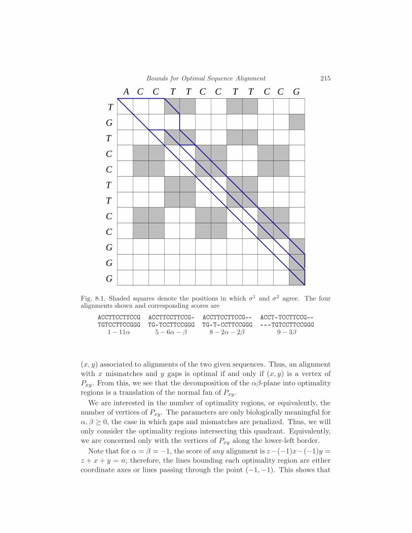
Bounds for Optimal Sequence Alignment 215
A C C C C C C
C
C
C
C
G
G
G
G
GT T T T
T
T
T
T
Fig. 8.1. Shaded squares denote the positions in which σ1 and σ2 agree. The fouralignments shown and corresponding scores are
ACCTTCCTTCCG ACCTTCCTTCCG- ACCTTCCTTCCG-- ACCT-TCCTTCCG--TGTCCTTCCGGG TG-TCCTTCCGGG TG-T-CCTTCCGGG - - -TGTCCTTCCGGG
1 − 11α 5 − 6α− β 8 − 2α− 2β 9 − 3β
(x, y) associated to alignments of the two given sequences. Thus, an alignment
with x mismatches and y gaps is optimal if and only if (x, y) is a vertex of
Pxy. From this, we see that the decomposition of the αβ-plane into optimality
regions is a translation of the normal fan of Pxy.
We are interested in the number of optimality regions, or equivalently, the
number of vertices of Pxy. The parameters are only biologically meaningful for
α, β ≥ 0, the case in which gaps and mismatches are penalized. Thus, we will
only consider the optimality regions intersecting this quadrant. Equivalently,
we are concerned only with the vertices of Pxy along the lower-left border.
Note that for α = β = −1, the score of any alignment is z−(−1)x−(−1)y =
z + x+ y = n; therefore, the lines bounding each optimality region are either
coordinate axes or lines passing through the point (−1,−1). This shows that

216 S. Elizalde and F. Lam
0
3 2
1
β
αFig. 8.2. Decomposition of the parameter space by sequences ACCTTCCTTCCG andACCTTCCTTCCG from Figure 8.1. The boundaries of the regions are given by the coor-dinate axes and the lines β = 1 + 2α, β = 3 + 4α and β = 4 + 5α.
all boundary lines of optimality regions are either coordinate axes or lines of
the form β = c+ (c+ 1)α for some constant c ([Gusfield et al., 1994]).
The polygon Pxy is a projection of the convex hull of the points (x, y, z)
giving the number of mismatches, gaps and matches of each alignment. All
these points lie on the plane x+ y + z = n and their convex hull is a polygon
which we denote P . We call P the alignment polygon. One obtains polygons
combinatorially equivalent to P and Pxy by projecting onto the xz-plane or
the yz-plane instead. It will be convenient for us to consider the projection
onto the yz-plane, which we denote Pyz .
8.2.1 The structure of the alignment polygon
The polygon Pyz is obtained by taking the convex hull of the points (y, z)
whose coordinates are the number of gaps and the number of matches of each
alignment of the two given sequences. Note that any mismatch of an alignment
can be replaced with two spaces, one in each sequence, without changing the
rest of the alignment. If we perform such a replacement in an alignment of
type (x, y, z), we obtain an alignment of type (x− 1, y+ 1, z). By replacing all
mismatches with gaps we obtain an alignment of type (0, x+y, z) = (0, n−z, z).

Bounds for Optimal Sequence Alignment 217
Similarly, replacing a match with two spaces in an alignment of type (x, y, z)
yields one of type (x, y+1, z−1), and performing all such replacements results
in an alignment of type (x, n− x, 0). Note however that the replacement of a
match with spaces never gives an optimal alignment for nonnegative values of
α and β.
From this, we see that if a point (y, z) inside Pyz comes from an alignment,
then the points (y + 1, z) and (y + 1, z − 1) must also come from alignments.
A natural question is whether all lattice points (i.e., points with integral coor-
dinates) inside Pyz come from alignments. We will see in the construction of
Proposition 9.2 that this is not the case in general. This means that there are
instances in which a lattice point (y′, z′) lies inside the convex hull of points
corresponding to alignments, but there is no alignment with y′ gaps and z′
matches.
From the above observation, it follows that P has an edge joining the ver-
tices (0, n, 0) and (0, n − zmax, zmax), where zmax is the maximum number of
matches in any alignment of the two given sequences. Similarly, P has an edge
joining (0, n, 0) and (xmax, n − xmax, 0), where xmax is the maximum number
of mismatches in any alignment. The alignment with no gaps also gives a
vertex of P , which we denote v0 = (x0, 0, z0). Going around P starting from
v0 in the direction where z increases, we label the vertices v1, v2, . . . , vr =
(0, n− zmax, zmax), vr+1 = (0, n, 0), vr+2 = (xmax, n− xmax, 0), . . .
x
y
z
y
z
Fig. 8.3. The alignment polygon P for the sequences in Figure 8.1 and its projec-tion Pyz.
For the meaningful values of the parameters, optimal alignments correspond
to the vertices v0, v1, . . . , vr. We call them relevant vertices of P . For vi =
(xi, yi, zi), we have
z0 < z1 < · · · < zr−1 ≤ zr = zmax,

218 S. Elizalde and F. Lam
0 = y0 < y1 < · · · < yr−1 < yr = n− zmax,
x0 > x1 > · · · > xr−1 > xr = 0.
Each vertex corresponds to an optimality region in the first quadrant of the
αβ-plane. For sequences σ1, σ2, we define g(σ1, σ2) = r+1 to be the number of
such optimality regions. Note that g(σ1, σ2) also equals the number of relevant
vertices of P , and the number of equivalence classes of optimal alignments of
σ1 and σ2 for nonnegative values of α and β.
Let Σ be a fixed alphabet (which can be finite or infinite). We define
fΣ(n) = maxσ1,σ2∈Σng(σ1, σ2).
In other words, fΣ(n) is the maximum number of optimality regions in the
decomposition of the first quadrant induced by a pair of sequences of length n
in the alphabet Σ. We are interested in bounds on fΣ(n).
8.3 Known bounds
The first nontrivial upper bound on fΣ(n) was given in [Gusfield et al., 1994],
where it was shown that fΣ(n) = O(n2/3) for any alphabet Σ (finite or infi-
nite). The more precise bound fΣ(n) = 3(n/2π)2/3 +O(n1/3 logn) is shown in
[Fernandez-Baca et al., 2002], and an example is given for which the bound is
tight if Σ is an infinite alphabet.
The idea used in [Fernandez-Baca et al., 2002] to establish the upper bound
uses the fact that the slopes of the segments connecting pairs of consecutive
relevant vertices of Pyz must be all different. The bound is obtained by calcu-
lating the maximum number of different rational numbers such that the sum
of all the numerators and denominators is at most n. To show that this bound
is tight for an infinite alphabet, for every n, they construct a pair of sequences
of length n for which the above bound on the number of different slopes be-
tween consecutive vertices of Pyz is attained. In their construction, the number
of different symbols that appear in the sequences of length n grows linearly
in n. It is an interesting question whether a similar Ω(n2/3) bound can be
achieved using fewer symbols, even if the number of symbols tends to infinity
as n increases.
This lower bound example only works when the alphabet Σ is infinite. How-
ever, biological sequences encountered in practice are over a finite alphabet,
usually the 4-letter alphabet A, C, G, T. For finite alphabets Σ, the asymp-
totic behavior of fΣ(n) is not known. The upper bound fΣ(n) ≤ 3(n/2π)2/3 +
O(n1/3 logn) seems to be far from the actual value in the case of a finite al-
phabet Σ.
Bounds for Optimal Sequence Alignment 219
8.4 The Square Root Conjecture
In the case of a binary alphabet Σ = 0, 1, for any n, there is a pair of
sequences of length n over Σ such that the number of equivalence classes of
optimal alignments is Ω(√n) ([Fernandez-Baca et al., 2002]). More precisely,
if we let s(n) = s be the largest integer such that s(s − 1)/2 ≤ n, then the
number of relevant vertices of the polygon P corresponding to the constructed
sequences of length n is s(n). This shows that f0,1(n) ≥ s(n) = Ω(√n).
Clearly, for any alphabet Σ of size |Σ| ≥ 2, the same construction using only
two symbols also shows fΣ(n) ≥ s(n) = Ω(√n). For a finite alphabet, the
best known bounds are fΣ(n) = Ω(√n) and fΣ(n) = O(n2/3). It is an open
problem to close this gap. We believe that the actual asymptotic behavior of
f0,1(n) is given by the lower bound.
Conjecture 8.1 f0,1(n) = Θ(√n).
It is clear that increasing the number of symbols in the alphabet Σ cre-
ates a larger number of possible pairs of sequences. In particular, we have
that fΣ′(n) ≥ fΣ(n) whenever |Σ′| ≥ |Σ|. Intuitively, a larger alphabet gives
more freedom on the different alignment polygons that arise, which potentially
increases the upper bound on the number of relevant vertices.
This is indeed the case in practice, as the following example shows. Let
Σ = 0, 1 be the binary alphabet, and let Σ′ = w1, w2, . . . , w6. Take a pair
of sequences of length n = 9 over Σ′ as follows: σ1 = w1w2w3w4w5w5w5w5w5,
σ2 = w6w1w2w6w3w6w6w4w6 (note that this construction is similar to the one
in Figure 8.4). Then, the alignment polygon has 5 relevant vertices, namely
v0 = (9, 0, 0), v1 = (6, 1, 2), v2 = (4, 2, 3), v3 = (1, 4, 4) and v4 = (0, 5, 4). It is
not hard to see that in fact fΣ′(n) = 5. However, one can check by exhaustive
computer search that there is no pair of binary sequences of length 9 such that
their alignment polytope has 5 relevant vertices. Thus, f0,1(n) = 4 < fΣ′(n).
In contrast to this result, the construction that gives the best known lower
bound Ω(√n) for finite alphabets is in fact over the binary alphabet. Thus,
one interesting question is whether the bounds on fΣ(n) are asymptotically
the same for all finite alphabets. In particular, it is an open question whether
an improved upper bound in the case of the binary alphabet would imply an
improved upper bound in the case of a finite alphabet.
One possible approach to reduce from the finite alphabet case to the binary
alphabet case is to consider the sequences σ1 and σ2 under all maps π : Σ →0, 1. There are 2k such maps, which we denote by πj, j = 1, . . . , 2k. For
each j, let P jxy be the convex hull of the points (x, y) giving the number of
mismatches and gaps of the alignments of sequences π(σ1) and π(σ2). We
would like to relate the vertices of Pxy to the vertices of P jxy.
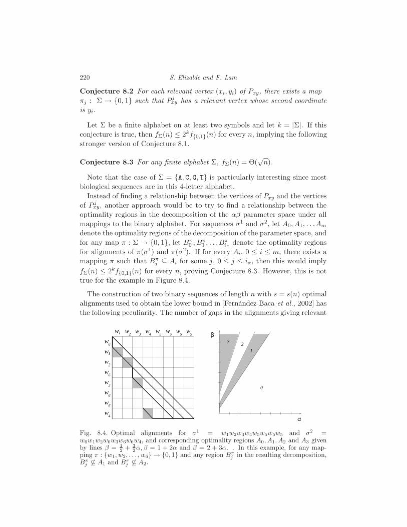
220 S. Elizalde and F. Lam
Conjecture 8.2 For each relevant vertex (xi, yi) of Pxy, there exists a map
πj : Σ → 0, 1 such that Pjxy has a relevant vertex whose second coordinate
is yi.
Let Σ be a finite alphabet on at least two symbols and let k = |Σ|. If this
conjecture is true, then fΣ(n) ≤ 2kf0,1(n) for every n, implying the following
stronger version of Conjecture 8.1.
Conjecture 8.3 For any finite alphabet Σ, fΣ(n) = Θ(√n).
Note that the case of Σ = A, C, G, T is particularly interesting since most
biological sequences are in this 4-letter alphabet.
Instead of finding a relationship between the vertices of Pxy and the vertices
of P jxy, another approach would be to try to find a relationship between the
optimality regions in the decomposition of the αβ parameter space under all
mappings to the binary alphabet. For sequences σ1 and σ2, let A0, A1, . . .Am
denote the optimality regions of the decomposition of the parameter space, and
for any map π : Σ → 0, 1, let Bπ0 , B
π1 , . . .B
πiπ denote the optimality regions
for alignments of π(σ1) and π(σ2). If for every Ai, 0 ≤ i ≤ m, there exists a
mapping π such that Bπj ⊆ Ai for some j, 0 ≤ j ≤ iπ, then this would imply
fΣ(n) ≤ 2kf0,1(n) for every n, proving Conjecture 8.3. However, this is not
true for the example in Figure 8.4.
The construction of two binary sequences of length n with s = s(n) optimal
alignments used to obtain the lower bound in [Fernandez-Baca et al., 2002] has
the following peculiarity. The number of gaps in the alignments giving relevant
w4
w5
w5
w5
w5
w4
w6
w6
w3
w6
w2
w1
w6
w1 w2
w3
0
β
α
1
23
Fig. 8.4. Optimal alignments for σ1 = w1w2w3w4w5w5w5w5 and σ2 =w6w1w2w6w3w6w6w4, and corresponding optimality regions A0, A1, A2 and A3 givenby lines β = 1
2 + 32α, β = 1 + 2α and β = 2 + 3α. . In this example, for any map-
ping π : w1, w2, . . . , w6 → 0, 1 and any region Bπj in the resulting decomposition,
Bπj 6⊆ A1 and Bπ
j 6⊆ A2.

Bounds for Optimal Sequence Alignment 221
vertices of the alignment polygon P are y0 = 0, y1 = 1, y2 = 2, . . . , ys−2 =
s − 2 (see Figure 8.5).
y
x
z
z
y
Fig. 8.5. The alignment polygon P for binary sequences of length n = 15 with s(n) = 6relevant vertices.
The slopes between consecutive relevant vertices in the projected alignment
polygon Pyz are then s, s − 1, s − 2, . . . , 1, 0. In particular, all the slopes are
integral. If this was true of all alignment polytopes coming from binary se-
quences, then Conjecture 8.1 would follow, because the maximum number of
different integral slopes in Pyz is s(n). However, it is not the case in general
that the slopes obtained from binary sequences are always integral.
The smallest counterexample is given by the pair of sequences σ1 = 001011
and σ2 = 111000. The vertices of the corresponding polytope Pyz are (0, 2),
(3, 3), (6, 0) and (10). The slope between the first two vertices is 1/3, which
shows that not all slopes are integral. In fact, it follows from the proof of
Proposition 9.3 that the situation is quite the opposite. We will see in the
next chapter that for any positive integers u, v with u < v, one can construct a
pair of binary sequences of length at most 6v−2u such that the corresponding
(projected) alignment polytope Pyz has a slope u/v between two consecutive
relevant vertices.
9
Inference Functions
Sergi Elizalde
Some of the statistical models introduced in Chapter 1 have the feature that,
aside from the observed data, there is hidden information that cannot be deter-
mined from an observation. These are called observed models, and particular
examples of them are the hidden Markov model and the hidden tree model.
A natural problem in such models is to determine, given a particular observa-
tion, what is the most likely hidden data (which is called explanation) for that
observation. Any fixed values of the parameters determine a way to assign an
explanation to each possible observation. A map obtained in this way is called
an inference function.
Examples of inference functions include gene finding functions. These are
used to determine what parts of a DNA sequence correspond to exons, which
will be translated into proteins, and what parts are introns, which will get
spliced out before the translation. They are inference functions of the hidden
Markov model described in Section 4.4. An observation in this model is a
sequence in the alphabet Σ′ = A, C, G, T.
9.1 What is an inference function?
Let us introduce some notation and make the definition more formal. Consider
a graphical model (as defined in Section 1.5) with n observed random variables
Y1, Y2, . . . , Yn, and q hidden random variables X1, X2, . . . , Xq. To simplify the
notation, we make the assumption, which is often the case in practice, that
all the observed variables are on the same finite alphabet Σ′, and that all the
hidden variables are on the finite alphabet Σ. The state space is then (Σ′)n. Let
l = |Σ| and l′ = |Σ′|. Let d be the number of parameters of the model, which
we denote θ1, θ2, . . . , θd. They express transition probabilities between states.
The model is represented by a positive polynomial map f : Rd −→ R(l′)n. For
each observation τ ∈ (Σ′)n, the corresponding coordinate fτ is a polynomial in
θ1, θ2, . . . , θd which gives the probability of making the particular observation τ .
222

Inference Functions 223
Thus, we have fτ = Prob(Y = τ) =∑
h∈Σq Prob(X = h,Y = τ), where each
summand Prob(X = h,Y = τ) is a monomial in the parameters θ1, θ2, . . . , θd.
For fixed values of the parameters, the basic inference problem is to deter-
mine, for each given observation τ , the value h ∈ Σq of the hidden data that
maximizes Prob(X = h|Y = τ). A solution to this optimization problem is
denoted h and is called an explanation of the observation τ . Each choice of
parameters (θ1, θ2, . . . , θd) defines an inference function τ 7→ h from the set of
observations (Σ′)n to the set of explanations Σq. A brief discussion of inference
functions and their geometric interpretation in terms of the tropicalization of
the polynomial map f was given at the end of Section 3.4.
It is possible that there is more than one value of h attaining the maximum
of Prob(X = h|Y = τ). In this case, for simplicity, we will pick only one such
explanation, according to some consistent tie-breaking rule decided ahead of
time. For example, we can pick the least such h in some given total order of
the set Σq of hidden states. Another alternative would be to define inference
functions as maps from (Σ′)n to subsets of Σq. This would not affect the
results of this chapter, so for the sake of simplicity we consider only inference
functions as defined above.
It is important to observe that the total number of functions (Σ′)n −→Σq is (lq)(l
′)n= lq(l
′)n, which is doubly-exponential in the length n of the
observations. However, most of these are not inference functions for any value
of the parameters. In this chapter we give an upper bound on the number of
inference functions of a graphical model.
We finish this section with some more notation that will be used in the
chapter. We denote by E the number of edges of the underlying graph of the
graphical model. The logarithms of the model parameters will be denoted by
vi = log(θi).
The coordinates of our model are polynomials of the form fτ (θ1, θ2, . . . , θd) =∑i θ
a1,i
1 θa2,i
2 · · ·θad,i
d . Recall from Section 2.3 that the Newton polytope of such
a polynomial is defined as the convex hull in Rd of the exponent vectors
(a1,i, a2,i, . . . , ad,i). We denote the Newton polytope of fτ by NP(fτ ), and
its normal fan by N (NP(fτ )).
Recall also that that the Minkowski sum of two polytopes P and P ′ is
P ⊙ P ′ := x + x′ : x ∈ P, x′ ∈ P ′. The Newton polytope of the map
f : Rd −→ R(l′)nis defined as the Minkowski sum of the individual Newton
polytopes of its coordinates, namely NP(f) :=⊙
τ∈(Σ′)n NP(fτ ).
9.2 The Few Inference Functions Theorem
For fixed parameters, the inference problem of finding the explanation h that
maximizes Prob(X = h|Y = τ) is equivalent to identifying the monomial

224 S. Elizalde
θa1,i
1 θa2,i
2 · · ·θad,i
d of fτ with maximum value. Since the logarithm is a monotone
increasing function, the sought monomial also maximizes the quantity
log(θa1,i
1 θa2,i
2 · · ·θad,i
d ) = a1,i log(θ1) + a2,i log(θ2) + . . .+ ad,i log(θd)
= a1,iv1 + a2,iv2 + . . .+ ad,ivd.
This is equivalent to the fact that the corresponding vertex (a1,i, a2,i, . . . , ad,i)
of the Newton polytope NP(fτ ) maximizes the linear expression v1x1 + . . .+
vdxd. Thus, the inference problem for fixed parameters becomes a linear pro-
gramming problem.
Each choice of the parameters θ = (θ1, θ2, . . . , θd) determines an inference
function. If v = (v1, v2, . . . , vd) is the vector in Rd with coordinates vi =
log(θi), then we denote the corresponding inference function by
Φv : (Σ′)n −→ Σq.
For each observation τ ∈ (Σ′)n, its explanation Φv(τ) is given by the vertex of
NP(fτ ) that is maximal in the direction of the vector v. Note that for certain
values of the parameters there may be more than one vertex attaining the
maximum, if v is perpendicular to a face of NP(fτ ). It is also possible that the
same point (a1,i, a2,i, . . . , ad,i) in the polytope corresponds to several different
values of the hidden data. In both cases, we pick the explanation according to
the tie-braking rule decided ahead of time. This simplification does not affect
the asymptotic number of inference functions.
Different values of θ yield different directions v, which give possibly different
inference functions. We are interested in bounding the number of different
inference functions that a graphical model can have. The next theorem states
that the number of inference functions grows polynomially in the complexity of
the graphical model. In particular, very few of the lq(l′)n
functions (Σ′)n −→ Σq
are inference functions.
Theorem 9.1 (The Few Inference Functions Theorem) Let d be a fixed
positive integer. Consider a graphical model with d parameters, and let E be
the number of edges of the underlying graph. Then, the number of inference
functions of the model is at most
O(Ed2(d−1)/2).
Before proving this theorem, observe that the number E of edges depends
on the number n of observed random variables. In most graphical models, E
is a linear function of n, so the bound becomes O(nd2(d−1)/2). For example,
the hidden Markov model has E = 2n− 1 edges.
Proof We have seen that an inference function is specified by a choice of the
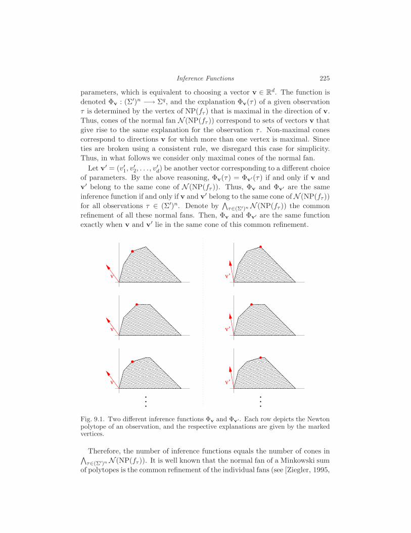
Inference Functions 225
parameters, which is equivalent to choosing a vector v ∈ Rd. The function is
denoted Φv : (Σ′)n −→ Σq, and the explanation Φv(τ) of a given observation
τ is determined by the vertex of NP(fτ ) that is maximal in the direction of v.
Thus, cones of the normal fan N (NP(fτ )) correspond to sets of vectors v that
give rise to the same explanation for the observation τ . Non-maximal cones
correspond to directions v for which more than one vertex is maximal. Since
ties are broken using a consistent rule, we disregard this case for simplicity.
Thus, in what follows we consider only maximal cones of the normal fan.
Let v′ = (v′1, v′2, . . . , v
′d) be another vector corresponding to a different choice
of parameters. By the above reasoning, Φv(τ) = Φv′(τ) if and only if v and
v′ belong to the same cone of N (NP(fτ )). Thus, Φv and Φv′ are the same
inference function if and only if v and v′ belong to the same cone of N (NP(fτ ))
for all observations τ ∈ (Σ′)n. Denote by∧
τ∈(Σ′)n N (NP(fτ )) the common
refinement of all these normal fans. Then, Φv and Φv′ are the same function
exactly when v and v′ lie in the same cone of this common refinement.
v v’
v’v
v v’
Fig. 9.1. Two different inference functions Φv and Φv′. Each row depicts the Newton
polytope of an observation, and the respective explanations are given by the markedvertices.
Therefore, the number of inference functions equals the number of cones in∧τ∈(Σ′)n N (NP(fτ )). It is well known that the normal fan of a Minkowski sum
of polytopes is the common refinement of the individual fans (see [Ziegler, 1995,
226 S. Elizalde
Proposition 7.12]). In our case, the common refinement is the normal fan of
NP(f) =⊙
τ∈(Σ′)n NP(fτ ), the Minkowski sum of the polytopes NP(fτ ) for all
observations τ . Thus, our goal is to bound the number of vertices of NP(f).
Note that for each τ , the polytope NP(fτ ) is contained in the cube [0, E]d.
This is because each parameter θi can appear as a factor of a monomial of fτ
at most E times. Besides, the vertices of NP(fτ ) have integral coordinates,
because they are exponent vectors. Polytopes whose vertices have integral
coordinates are called lattice polytopes. It follows that the edges of NP(fτ ) are
given by vectors where each coordinate is an integer between −E and E. Each
edge of NP(f) has the same direction as an edge of one of its summands NP(fτ ).
Therefore, the normal vector of any facet of NP(f) is obtained as the vector
perpendicular to d − 1 linearly independent vectors in [−E,E]d with integral
coordinates. Since there are only O(Ed) such vectors, the normal vectors of
the facets of NP(fτ ) can take at most O(Ed(d−1)) different directions.
This implies that NP(f) has at most O(Ed(d−1)) facets. By the Upper Bound
Theorem (see [McMullen, 1971]), a d-dimensional polytope with N facets can
have at most O(N d/2) vertices. Thus, the number of vertices of NP(f), and
hence the number of inference functions of the graphical model, is bounded
from above by O(Ed2(d−1)/2).
9.3 Inference functions for sequence alignment
We now show how Theorem 9.1 can be applied to give a tight bound on the
number of inference functions of the model for sequence alignment used in
Chapter 8. Recall the sequence alignment problem from Section 2.2, which
consists in finding the best alignment between two sequences. Given two strings
σ1 and σ2 of lengths n1 and n2 respectively, an alignment is a pair of equal
length strings (µ1, µ2) obtained from σ1, σ2 by inserting “−” characters in
such a way that there is no position in which both µ1 and µ2 have a “−”. A
match is a position where µ1 and µ2 have the same character, a mismatch is a
position where µ1 and µ2 have different characters, and a space is a position
in which one of µ1 and µ2 has a space. A simple scoring scheme consists of
two parameters α and β denoting mismatch and space penalties respectively.
The score of an alignment with z matches, x mismatches, and y spaces is then
z−xα− yβ. Observe that these numbers always satisfy 2z+2x+ y = n1 +n2.
For pairs of sequences of equal length, this is the same scoring scheme used in
Chapter 8, with y = 2y and β = β/2. In this case, y is called the number of
gaps, which is half the number of spaces, and β is the penalty for a gap.
This 2-parameter model for sequence alignment is a particular case of the
pair hidden Markov model discussed in Section 2.2. The problem of determin-
ing the highest scoring alignment for given values of α and β is equivalent to
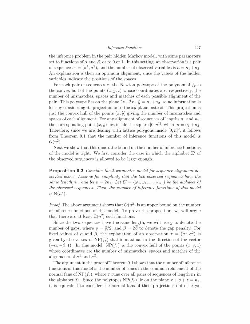
Inference Functions 227
the inference problem in the pair hidden Markov model, with some parameters
set to functions of α and β, or to 0 or 1. In this setting, an observation is a pair
of sequences τ = (σ1, σ2), and the number of observed variables is n = n1 +n2.
An explanation is then an optimum alignment, since the values of the hidden
variables indicate the positions of the spaces.
For each pair of sequences τ , the Newton polytope of the polynomial fτ is
the convex hull of the points (x, y, z) whose coordinates are, respectively, the
number of mismatches, spaces and matches of each possible alignment of the
pair. This polytope lies on the plane 2z+2x+ y = n1+n2, so no information is
lost by considering its projection onto the xy-plane instead. This projection is
just the convex hull of the points (x, y) giving the number of mismatches and
spaces of each alignment. For any alignment of sequences of lengths n1 and n2,
the corresponding point (x, y) lies inside the square [0, n]2, where n = n1 +n2.
Therefore, since we are dealing with lattice polygons inside [0, n]2, it follows
from Theorem 9.1 that the number of inference functions of this model is
O(n2).
Next we show that this quadratic bound on the number of inference functions
of the model is tight. We first consider the case in which the alphabet Σ′ of
the observed sequences is allowed to be large enough.
Proposition 9.2 Consider the 2-parameter model for sequence alignment de-
scribed above. Assume for simplicity that the two observed sequences have the
same length n1, and let n = 2n1. Let Σ′ = ω0, ω1, . . . , ωn1 be the alphabet of
the observed sequences. Then, the number of inference functions of this model
is Θ(n2).
Proof The above argument shows that O(n2) is an upper bound on the number
of inference functions of the model. To prove the proposition, we will argue
that there are at least Ω(n2) such functions.
Since the two sequences have the same length, we will use y to denote the
number of gaps, where y = y/2, and β = 2β to denote the gap penalty. For
fixed values of α and β, the explanation of an observation τ = (σ1, σ2) is
given by the vertex of NP(fτ ) that is maximal in the direction of the vector
(−α,−β, 1). In this model, NP(fτ ) is the convex hull of the points (x, y, z)
whose coordinates are the number of mismatches, spaces and matches of the
alignments of σ1 and σ2.
The argument in the proof of Theorem 9.1 shows that the number of inference
functions of this model is the number of cones in the common refinement of the
normal fans of NP(fτ ), where τ runs over all pairs of sequences of length n1 in
the alphabet Σ′. Since the polytopes NP(fτ ) lie on the plane x+ y + z = n1,
it is equivalent to consider the normal fans of their projections onto the yz-
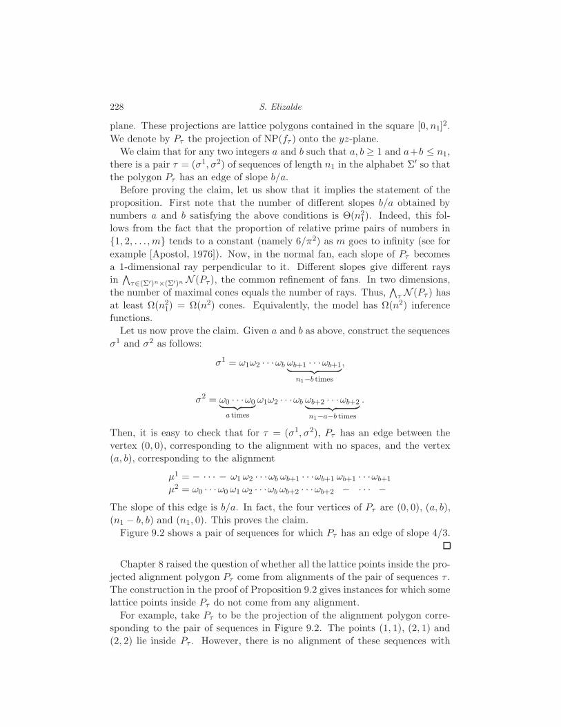
228 S. Elizalde
plane. These projections are lattice polygons contained in the square [0, n1]2.
We denote by Pτ the projection of NP(fτ ) onto the yz-plane.
We claim that for any two integers a and b such that a, b ≥ 1 and a+b ≤ n1,
there is a pair τ = (σ1, σ2) of sequences of length n1 in the alphabet Σ′ so that
the polygon Pτ has an edge of slope b/a.
Before proving the claim, let us show that it implies the statement of the
proposition. First note that the number of different slopes b/a obtained by
numbers a and b satisfying the above conditions is Θ(n21). Indeed, this fol-
lows from the fact that the proportion of relative prime pairs of numbers in
1, 2, . . . , m tends to a constant (namely 6/π2) as m goes to infinity (see for
example [Apostol, 1976]). Now, in the normal fan, each slope of Pτ becomes
a 1-dimensional ray perpendicular to it. Different slopes give different rays
in∧
τ∈(Σ′)n×(Σ′)n N (Pτ ), the common refinement of fans. In two dimensions,
the number of maximal cones equals the number of rays. Thus,∧
τ N (Pτ ) has
at least Ω(n21) = Ω(n2) cones. Equivalently, the model has Ω(n2) inference
functions.
Let us now prove the claim. Given a and b as above, construct the sequences
σ1 and σ2 as follows:
σ1 = ω1ω2 · · ·ωb ωb+1 · · ·ωb+1︸ ︷︷ ︸n1−b times
,
σ2 = ω0 · · ·ω0︸ ︷︷ ︸a times
ω1ω2 · · ·ωb ωb+2 · · ·ωb+2︸ ︷︷ ︸n1−a−b times
.
Then, it is easy to check that for τ = (σ1, σ2), Pτ has an edge between the
vertex (0, 0), corresponding to the alignment with no spaces, and the vertex
(a, b), corresponding to the alignment
µ1 = − · · · − ω1 ω2 · · ·ωb ωb+1 · · ·ωb+1 ωb+1 · · ·ωb+1
µ2 = ω0 · · ·ω0 ω1 ω2 · · ·ωb ωb+2 · · ·ωb+2 − · · · −The slope of this edge is b/a. In fact, the four vertices of Pτ are (0, 0), (a, b),
(n1 − b, b) and (n1, 0). This proves the claim.
Figure 9.2 shows a pair of sequences for which Pτ has an edge of slope 4/3.
Chapter 8 raised the question of whether all the lattice points inside the pro-
jected alignment polygon Pτ come from alignments of the pair of sequences τ .
The construction in the proof of Proposition 9.2 gives instances for which some
lattice points inside Pτ do not come from any alignment.
For example, take Pτ to be the projection of the alignment polygon corre-
sponding to the pair of sequences in Figure 9.2. The points (1, 1), (2, 1) and
(2, 2) lie inside Pτ . However, there is no alignment of these sequences with
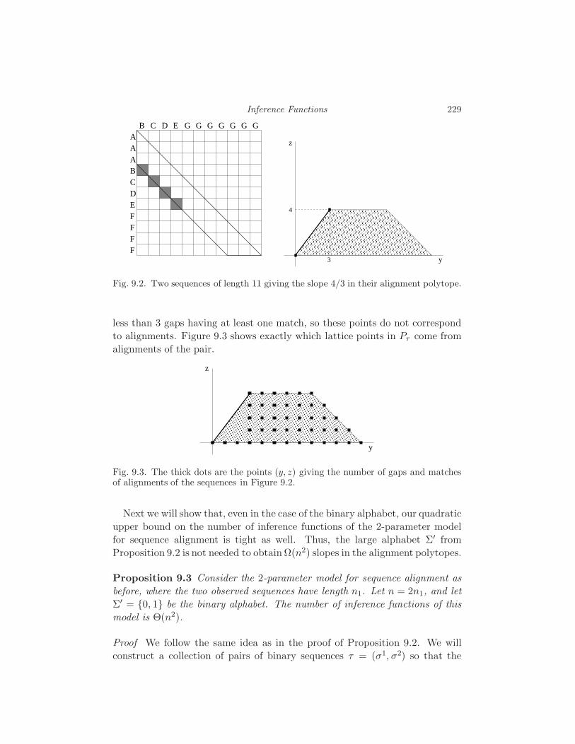
Inference Functions 229
4
z
y
AAABCDEFFFF
CB D E G G G G G GG
3
Fig. 9.2. Two sequences of length 11 giving the slope 4/3 in their alignment polytope.
less than 3 gaps having at least one match, so these points do not correspond
to alignments. Figure 9.3 shows exactly which lattice points in Pτ come from
alignments of the pair.
y
z
Fig. 9.3. The thick dots are the points (y, z) giving the number of gaps and matchesof alignments of the sequences in Figure 9.2.
Next we will show that, even in the case of the binary alphabet, our quadratic
upper bound on the number of inference functions of the 2-parameter model
for sequence alignment is tight as well. Thus, the large alphabet Σ′ from
Proposition 9.2 is not needed to obtain Ω(n2) slopes in the alignment polytopes.
Proposition 9.3 Consider the 2-parameter model for sequence alignment as
before, where the two observed sequences have length n1. Let n = 2n1, and let
Σ′ = 0, 1 be the binary alphabet. The number of inference functions of this
model is Θ(n2).
Proof We follow the same idea as in the proof of Proposition 9.2. We will
construct a collection of pairs of binary sequences τ = (σ1, σ2) so that the
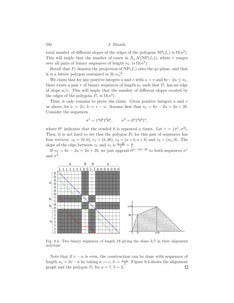
230 S. Elizalde
total number of different slopes of the edges of the polygons NP(fτ ) is Ω(n2).
This will imply that the number of cones in∧
τ N (NP(fτ )), where τ ranges
over all pairs of binary sequences of length n1, is Ω(n2).
Recall that Pτ denotes the projection of NP(fτ ) onto the yz-plane, and that
it is a lattice polygon contained in [0, n1]2.
We claim that for any positive integers u and v with u < v and 6v−2u ≤ n1,
there exists a pair τ of binary sequences of length n1 such that Pτ has an edge
of slope u/v. This will imply that the number of different slopes created by
the edges of the polygons Pτ is Ω(n2).
Thus, it only remains to prove the claim. Given positive integers u and v
as above, let a := 2v, b := v − u. Assume first that n1 = 6v − 2u = 2a + 2b.
Consider the sequences
σ1 = 1a0b1b0a, σ2 = 0a1b0b1a,
where 0a indicates that the symbol 0 is repeated a times. Let τ = (σ1, σ2).
Then, it is not hard to see that the polygon Pτ for this pair of sequences has
four vertices: v0 = (0, 0), v1 = (b, 3b), v2 = (a+ b, a+ b) and v3 = (n1, 0). The
slope of the edge between v1 and v2 is a−2ba = u
v .
If n1 > 6v − 2u = 2a+ 2b, we just append 0n1−2a−2b to both sequences σ1
and σ2.
1 11 1 1 11 0 0 1 1 0 0 0 0 0 0 0000000011001111111
a ab b
b
b
a
a
b a+b
3b
a+b
Fig. 9.4. Two binary sequences of length 18 giving the slope 3/7 in their alignmentpolytope.
Note that if v − u is even, the construction can be done with sequences of
length n1 = 3v−u by taking a := v, b := v−u2 . Figure 9.4 shows the alignment
graph and the polygon Pτ for a = 7, b = 2.

Inference Functions 231
In most cases, one is interested only in those inference functions that are
biologically meaningful. In our case, meaningful values of the parameters occur
when α, β ≥ 0, which means that mismatches and spaces are penalized, instead
of rewarded. Sometimes one also requires that α ≤ β, which means that a
mismatch should be penalized less than two spaces. It is interesting to observe
that our constructions in the proofs of Propositions 9.2 and 9.3 not only show
that the total number of inference functions is Ω(n2), but also that the number
of biologically meaningful ones is still Ω(n2). This is because the different rays
created in our construction have a biologically meaningful direction in the
parameter space.
Let us now relate the results from this section with the bounds given in
the previous chapter. In Chapter 8 we saw that in the 2-parameter model for
sequence alignment, if τ is a pair of sequences of length n in an arbitrarily large
alphabet, then the polygon Pτ can have Θ(n2/3) vertices in the worst case. In
Proposition 9.2 we have shown that the Minkowski sum of these polygons for
all possible such observations τ , namely⊙
τ Pτ , has Θ(n2) vertices.
In the case where the alphabet for the sequences is binary (or more generally,
finite), in Chapter 8 we conjectured that the polygon Pτ can only have Θ(√n)
vertices at most. In Proposition 9.3 we have proved that the polygon⊙
τ Pτ ,
where τ runs over all pairs of binary sequences of length n, has Θ(n2) vertices
as well.
Having shown that the number of inference functions of a graphical model is
polynomial in the size of the model, an interesting next step would be to find
a way to precompute all the inference functions for given models and store
them in the memory. This would allow us to answer queries about a given
observation very efficiently.

10
Geometry of Markov Chains
Eric Kuo
This chapter discusses the differences between Viterbi sequences of Markov
chains and toric Markov chains. When the chains have 2 or 3 states, there
are some sequences that are Viterbi for a toric Markov chain, but not for any
Markov chain. However, when the chain has 4 or more states, the sets of Viterbi
sequences are identical for both Markov chains and toric Markov chains. We
also discuss maximal probability sequences for fully observed Markov models.
10.1 Viterbi Sequences
In this chapter, we number the states of an l-state Markov chain from 0 to
l − 1. Given a Markov chain M , the probability of a sequence is the product
of the initial probability of the first state and all the transition probabilities
between consecutive states. There are ln possible sequences of length n. A
Viterbi path of length n is a sequence of n states (containing n transitions)
with the highest probability. Viterbi paths of Markov chains can be computed
in polynomial time [Forney, 1973, Viterbi, 1967]. A Markov chain may have
more than one Viterbi path of length n; for instance, if 012010 is a Viterbi path
of length 6, then 010120 must also be a Viterbi path since both sequences have
the same initial state and the same set of transitions, only that they appear
in a different order. Two sequences are equivalent if their set of transitions are
the same. The Viterbi paths of a Markov chain might not be all equivalent.
Consider the Markov chain on l states that has a uniform initial distribution
and a uniform transition matrix (i.e. θij = 1l for all states i, j). Since each
sequence of length n has the same probability 1ln , every sequence is a Viterbi
path for this Markov chain.
If a sequence S and all others equivalent to S are the only Viterbi paths
of a Markov chain, then we call S a Viterbi sequence. A simple example of a
Viterbi sequence of length 4 is 0000 since it is the only Viterbi path for the
232

Geometry of Markov Chains 233
two-state Markov chain with transition matrix
θ =
(1 0
0 1
).
An example of a sequence that is not a Viterbi sequence is 0011. If 0011 were a
Viterbi sequence, then its probability must be greater than those of sequences
0001 and 0111. Since p0011 > p0001,
θ00θ01θ11 > θ200θ01,
from which we conclude θ11 > θ00. But from p0011p0111, we get
θ00θ01θ11 > θ01θ211,
from which we get θ00 > θ11, a contradiction.
We can similarly define Viterbi paths and sequences for toric Markov chains.
Recall that the transition matrix for a toric Markov chain is not necessarily
stochastic. Because of this fact, the set Tl of Viterbi sequences of l-state toric
Markov chains may be different from the set Vl of Viterbi sequences of l-state
(regular) Markov chains. Note that Vl is a subset of Tl since every Markov
chain is a toric Markov chain. We call the sequences in the set difference
Tl − Vl pseudo-Viterbi sequences. (For the rest of this article, the term Viterbi
path and sequence will refer to regular Markov chains; for toric Markov chains,
we call them toric Viterbi paths and sequences.
The main result in this article is that for l = 2 and 3, pseudo-Viterbi se-
quences exist. When l ≥ 4, there are no pseudo-Viterbi sequences; the sets of
Viterbi sequences and toric Viterbi sequences are equal.
To help prove these results, we will need to prove some general properties
about Viterbi sequences.
Proposition 10.1 If a Viterbi sequence S has two subsequences T1 and T2 of
length t that both begin with state q1 and end with state q2, then T1 and T2 are
equivalent sequences.
Proof Suppose that T1 and T2 are not equivalent subsequences. Then let S1 be
the sequence obtained by replacing T2 with T1 in S so that pS1 = pSpT1/pT2.
Similarly, let S2 be the sequence obtained by replacing T1 with T2 in S so that
pS2 = pSpT2/pT1. Since S is Viterbi and not equivalent to S1, we must have
pS > pS1, which implies pT2 > pT1. But since S is also not equivalent to S2,
we also have pS > pS2, which implies pT1 > pT2. This is a contradiction, so T1
and T2 must be equivalent.
As an example, 01020 is not a Viterbi sequence since 010 and 020 are non-

234 E. Kuo
A∗ 02m+1 (2m, 0, 0, 0) A∗ 02m+2 (2m+ 1, 0, 0, 0)B 02m1 (2m− 1, 1, 0, 0) B 02m+11 (2m, 1, 0, 0)C 0(01)m (1, m,m− 1, 0) C∗ 0(01)m0 (1, m,m, 0)D∗ (01)m1 (0, m,m− 1, 1) D (01)m10 (0, m,m, 1)E∗ (01)m0 (0, m,m, 0) E∗ (01)m+1 (0, m+ 1, m, 0)F 012m−10 (0, 1, 1, 2m− 2) F 012m0 (0, 1, 1, 2m− 1)G∗ 012m (0, 1, 0, 2m− 1) G∗ 012m+1 (0, 1, 0, 2m)
Table 10.1. Left: Toric Viterbi sequences of length 2m+ 1. Right: Toric
Viterbi sequences of length 2m+ 2. Starred sequences are Viterbi, unstarred
are pseudo-Viterbi.
equivalent subsequences of the same length beginning and ending with 0. Ei-
ther p01010 or p02020 will be greater than or equal to p01020.
The next proposition was illustrated with an earlier example, 0011.
Proposition 10.2 If a transition ii exists in a Viterbi sequence S, then no
other transition jj can appear in S, where j 6= i.
Proof Suppose S did contain transitions ii and jj. Consider the sequences
S1 where subsequence ii is replaced by i and jj is replaced by jjj. Since S is
Viterbi, we must have pS > pS1 , from which we conclude pii > pjj. However,
we can also create another sequence S2 in which ii is replaced with iii and jj is
replaced with j. Once again, pS > pS2, so pjj > pii, giving us a contradiction.
10.2 Two- and Three-State Markov Chains
For toric Markov chains on l = 2 states, there are seven toric Viterbi sequences
with initial state 0 when the length n ≥ 5. They are listed in Table 10.1.
Not all toric Viterbi sequences are Viterbi sequences. In fact, for each n > 3,
three sequences are pseudo-Viterbi because of the following proposition.
Proposition 10.3 No Viterbi sequence on two states can end with 001 or 110.
Proof Suppose that 001 is a Viterbi sequence. Then since p001 > p010, we
must have θ00 > θ10. Also, p001 > p000, so θ01 > θ00. Finally, p001 > p011, so
θ00 > θ11. But then
1 = θ00 + θ01 > θ10 + θ00 > θ10 + θ11 = 1,
which is a contradiction. Thus no Viterbi sequence can end with 001 (or by
symmetry, 110).
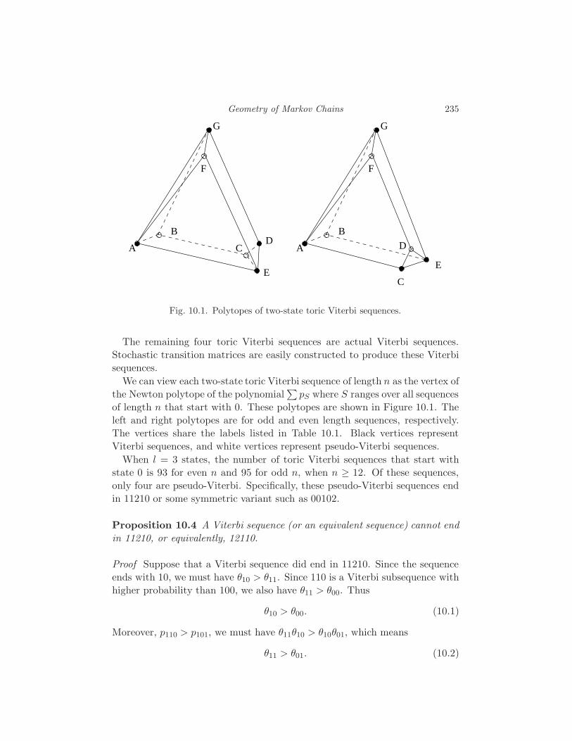
Geometry of Markov Chains 235
A
B
G
F
DC
E
C
A
B
E
G
F
D
Fig. 10.1. Polytopes of two-state toric Viterbi sequences.
The remaining four toric Viterbi sequences are actual Viterbi sequences.
Stochastic transition matrices are easily constructed to produce these Viterbi
sequences.
We can view each two-state toric Viterbi sequence of length n as the vertex of
the Newton polytope of the polynomial∑pS where S ranges over all sequences
of length n that start with 0. These polytopes are shown in Figure 10.1. The
left and right polytopes are for odd and even length sequences, respectively.
The vertices share the labels listed in Table 10.1. Black vertices represent
Viterbi sequences, and white vertices represent pseudo-Viterbi sequences.
When l = 3 states, the number of toric Viterbi sequences that start with
state 0 is 93 for even n and 95 for odd n, when n ≥ 12. Of these sequences,
only four are pseudo-Viterbi. Specifically, these pseudo-Viterbi sequences end
in 11210 or some symmetric variant such as 00102.
Proposition 10.4 A Viterbi sequence (or an equivalent sequence) cannot end
in 11210, or equivalently, 12110.
Proof Suppose that a Viterbi sequence did end in 11210. Since the sequence
ends with 10, we must have θ10 > θ11. Since 110 is a Viterbi subsequence with
higher probability than 100, we also have θ11 > θ00. Thus
θ10 > θ00. (10.1)
Moreover, p110 > p101, we must have θ11θ10 > θ10θ01, which means
θ11 > θ01. (10.2)
236 E. Kuo
Finally, 112 has higher probability than 102, so θ11θ12 > θ10θ02. Then
θ12 >θ10θ02
θ11> θ02 (10.3)
where we use the fact that θ10 > θ11. Thus
1 = θ10 + θ11 + θ12 > θ00 + θ01 + θ02 = 1 (10.4)
which is a contradiction.
However, 0212110 is a toric Viterbi sequence for the toric Markov chain with
the following transition matrix:
0 0 0.1
0.5 0.3 0.2
0 0.6 0
.
10.3 Markov Chains with Many States
Of the seven two-state toric Viterbi sequences of length n that start with state
0, three are pseudo-Viterbi sequences. Out of the 93 or 95 (depending on the
parity of n) three-state toric Viterbi sequences of length n starting with state
0, only four of them are pseudo-Viterbi sequences. So we might ask, how many
pseudo-Viterbi sequences exist as the number of states increases? The answer
lies in the following theorem:
Theorem 10.5 Every toric Viterbi sequence on l ≥ 4 states is a Viterbi se-
quence.
Proof In order to show that a min-weight sequence S (of length n) is Viterbi,
we need the following facts:
(i) For each state i, there exists another state j (which may be the same
as i) for which transition ij does not appear in S.
(ii) If the previous statement is true, then we can find a stochastic matrix
of transition probabilities whose Viterbi sequence of length n is S.
To prove the first fact, we assume there is a state q for which each transition
q0, q1, . . . , q(l− 1) exists at least once in S. Let’s assume q is state 0 (for we
could merely relabel the states in S). We can rearrange S so that the final l
appearances of state 0 take the form 001x102x203x3 . . .0(l−1)xl−1, where each
xi is a (possibly empty) string of states. Thus each transition 00, 01, . . . , 0(l−1)
appears exactly once in this subsequence, and we assume that l−1 is the state
that follows the last 0.
Since l ≥ 4, strings x1 and x2 must be followed by state 0. Strings x1 and
x2 cannot both be empty, for then p010 = p020, violating Proposition 10.1.
Geometry of Markov Chains 237
(Note that for l ≤ 3, this proof fails since x1 and x2 could both be empty.) So
suppose x1 is nonempty. The first state of x1 (immediately following state 1)
cannot be state 1, for then p00 = p11, violating Proposition 10.2. So it must
be some state other than 0 or 1; call it state r. We could rearrange S so that
transition 00 precedes transition 0r. Then within S we have two subsequences
00r and 01r, violating Proposition 10.1. This is a contradiction. Thus there
must be at least one state s that never follows state 0 in S.
To prove the second statement, we construct a stochastic transition matrix
for which S is a Viterbi sequence. Because of the first fact, we can assign every
transition ij in S a probability θij greater than 1/l. (Note that this would be
impossible in the cases 001 for l = 2 and 11210 for l = 3.) For each transition
ij that appears in S, we assign a probability θij between 1l + ǫ and 1
l + αǫ,
where1
l<
1
l+ ǫ <
1
l+ αǫ <
1
l − 1.
If ij is in S, then for the transitions ij ′ that are not in S, we can still let
0 < θij′ < 1/l.
Now if state i does not appear in S or only appears as the final state of S,
then each transition ij is assigned a probability θij not exceeding 1l +η, where
0 < η < ǫ. We attempt to choose α, ǫ, and η so that they satisfy the inequality
(1
l+ η
)(1
l+ αǫ
)n−2
<
(1
l+ ǫ
)n−2 (1
l+ αǫ
). (10.5)
The right hand side represents the minimum possible value for the probabil-
ity of S, for it has at least one transition with the maximum probability 1l +αǫ
while all the others have at least the minimum probability 1l +ǫ. The left hand
side represents the maximum probability any other sequence S ′ can attain in
which S ′ contains a transition not in S. At least one transition has probability
at most 1l + η, while the rest may have maximum probability 1
l + αǫ.
We show that we can choose values for α, ǫ, and η that satisfies the inequality.
If we set α = 1 and η = 0, the inequality is automatically satisfied, and thus
we can increment α and η very slightly and still satisfy the inequality.
Since S is a toric Viterbi sequence, there is a matrix θT for which S is the
toric Viterbi sequence. We then take logarithms so that wij = log θTij for each
transition ij for which θTij 6= 0. Let w1 and w2 be the minimum and maximum
values of wij, respectively, of all the transitions ij that appear in S. We then
let L(w) = aw + b (where a > 0) be the linear transformation that maps w1
to − log( 1l + αǫ) and w2 to − log( 1
l + ǫ). For each transition ij that appears
in S, we set θij such that
− log θij = L(wij) = awij + b. (10.6)

238 E. Kuo
In particular, if all of the transition in another sequence S ′ appears in S, we
have
n−1∑
i=1
L(wSiSi+1) = b(n− 1) + a∑
wSiSi+1
< b(n− 1) + a
n−1∑
i=1
wS′iS
′i+1
=n−1∑
i=1
L(wS′iS
′i+1
)
Note how for each ij in S,
1
l+ ǫ = exp(−L(w2)) ≤ θij = exp(−L(wij)) ≤ exp(−L(w1)) =
1
l+ αǫ.
If ij is a transition in S, then each transition starting with i that is not in S is
assigned a probability not exceeding 1l − ǫ
l−1 . The remaining probabilities are
assigned so that none of them exceed 1l + η.
We now demonstrate that θ is a stochastic matrix for which S is the only
Viterbi path. If sequence S ′ has a transition not in S, then pS is at least the
right-hand side of 10.5, and pS′ is at most the left-hand side of 10.5. Thus
pS > pS′ . If all the transitions in S ′ are in S, then
− log pS = −n−1∑
i=1
log θSiSi+1 =n−1∑
i=1
L(wSiSi+1 )
<
n−1∑
i=1
L(wS′iS
′i+1
)
= −n−1∑
i=1
log θS′iS
′i+1
= − log pS′ .
10.4 Fully Observed Markov Models
We turn our attention to the fully observed Markov model. The states of a
fully observed Markov model are represented by two alphabets Σ and Σ′ of l
and l′ letters, respectively. We parameterize the fully observed Markov model
by a pair of matrices (θ, θ′) with dimensions l × l and l × l′. The entry θij is
the transition probability from state i ∈ Σ to state j ∈ Σ. Entry θ′ij represents
a transition probability from i ∈ Σ to j ∈ Σ′.
The fully observed Markov model generates a pair of sequences S ∈ Σ∗
Geometry of Markov Chains 239
and T ∈ Σ′∗. Sequence S is generated just the same way that a regular
Markov chain with transition matrix θ would. Each state in T is generated
individually from the corresponding state in S with the transition matrix θ′.
Thus if Si = σ is the ith state in S, then the ith state of T would be Ti = σ′
with probability θ′σσ′ . We will call S the state sequence and T the output
sequence of a fully observed sequence (S, T ). A fully observed sequence (S, T )
of length n is generated by a fully observed Markov model with transitions
(θ, θ′) with probability
pS,T = π1θ′S1T1
n∏
i=2
θSi−1Siθ′SiTi
(10.7)
where π1 is the probability of the initial state S1.
In a fully observed Markov model, both transition matrices (θ, θ′) are stochas-
tic. When we don’t require either matrix to be stochastic, we call it a fully
observed toric Markov model.
We now define some terms referring to fully observed sequences of maximal
likelihood. A fully observed Viterbi path of length n of a fully observed Markov
model is the fully observed sequence (S, T ) of length n that the fully observed
Markov model generates with the highest probability. If (S, T ) and (S ′, T ′) are
two fully observed sequences for which each transition (i, j) ∈ Σ×Σ or (i, j ′) ∈Σ × Σ′ appears in each sequence pair an equal number of times, then we say
that (S, T ) and (S ′, T ′) are equivalent. If the only fully observed Viterbi paths
for a fully observed Markov model are (S, T ) and any equivalent sequences,
then (S, T ) is a fully observed Viterbi sequence. The pair (S, T ) will usually
represent the entire equivalence class of sequences. We analogously define a
fully observed toric Viterbi paths and sequences for fully observed toric Markov
models.
We make an immediate observation about fully observed Viterbi sequences:
Lemma 10.6 Let (S, T ) be a fully observed (toric) Viterbi sequence. If Si and
Sj are the same state in Σ, then Ti and Tj are the same state in Σ′.
Proof Suppose that Si = Sj, but Ti 6= Tj. We can create two additional output
sequences T ′ and T ′′ in which we set T ′i = T ′j = Ti and T ′′i = T ′′j = Tj. Then
since pS,T > pS,T ′, we must have
θ′SiTi> θ′SiT
′i= θ′SiTj
. (10.8)
Since we also have pS,T > pS,T ′′ , we must also have
θ′SjTj> θ′SjT ′′
j. (10.9)
240 E. Kuo
Since Si = Sj and T ′′j = Ti, we get
θ′SiTj> θ′SiTi
, (10.10)
contradicting (10.8).
So if state j ∈ Σ′ appears with state i ∈ Σ in a fully observed Viterbi
sequence (S, T ), then j appears in T with every instance of i in S.
We now prove some properties about the state sequence of a fully observed
toric Viterbi sequence.
Lemma 10.7 The state sequence of every fully observed toric Viterbi sequence
is a toric Viterbi sequence.
Proof Let S be the state sequence for the fully observed toric Viterbi sequence
(S, T ) of a fully observed Markov model M with matrices (θ, θ′). Now create
a new toric Markov chain M ′ with transition matrix φ such that
φij = maxkθijθ′jk. (10.11)
Now we show that S is also the only toric Viterbi path of M ′. Its probability
is greater than that of any other sequence S ′ since the probability of S ′ in the
Markov chain is equal to the maximum probability pS′,T ′ of all fully observed
sequences with state sequence S ′. The value pS′,T ′ is less than pS,T .
We finally deduce a criterion for determining whether a fully observed se-
quence is a fully observed Viterbi sequence.
Theorem 10.8 The state sequence S for a fully observed toric Viterbi se-
quence (S, T ) is a Viterbi sequence if and only if (S, T ) is also a fully observed
Viterbi sequence.
Proof Let S be a Viterbi sequence. Then there is a stochastic matrix θ for
which S is the only Viterbi path. We also create another stochastic matrix θ′
in which θ′ij = 1 whenever transition ij appears in (S, T ). (Recall from Lemma
10.6 that for each i, at most one output state j matches with i.) So for all
other fully observed Viterbi sequences (S ′, T ′),
pS,T = pS > pS′ ≥ pS′,T ′ . (10.12)
Thus (S, T ) is a fully observed Viterbi sequence for the fully observed Markov
model with matrices (θ, θ′).
To show the other direction, we assume that the state sequence S is not
a Viterbi sequence. However, we know that S is a toric Viterbi sequence by
Lemma 10.7. Thus S is a pseudo-Viterbi sequence. So there are two cases to
consider:
Geometry of Markov Chains 241
Case I: Σ = 0, 1, and S (or an equivalent sequence) ends with 001 (or
symmetrically, 110). Let A,B ∈ Σ′, and θ′0A and θ′1B are the maximal prob-
ability transitions from states 0 and 1 in θ′. (Note that A and B need not
be distinct.) Then since p001,AAB > p010,ABA, we must have θ00 > θ10. Also,
p001,AAB > p000,AAA, so θ01θ′1B > θ00θ
′0A. Finally, p001,AAB > p011,ABB, so
θ00θ′0A > θ11θ
′1B. Thus θ01θ
′1B > θ11θ
′1B , so θ01 > θ11. But then
1 = θ00 + θ01 > θ10 + θ11 = 1,
which is a contradiction. Thus S is not the state sequence of a fully observed
Viterbi sequence.
Case II: Σ = 0, 1, 2, and S (or an equivalent sequence) ends with 11210
(or any symmetric variant like 00102). Let A,B, C ∈ Σ′ such that θ′0A, θ′1B,
and θ′2C are the greatest probabilities for transitions from states 0, 1, and 2 in
θ′. (Once again, A, B, and C need not be distinct.) Since the sequence ends
with 10, we must have
θ10θ′0A > θ11θ
′1B. (10.13)
We also have p11210,BBCBA > p12100,BCBAA, which implies that
θ11θ′1B > θ00θ
′0A (10.14)
From inequalities 10.13 and 10.14, we conclude θ10θ′0A > θ00θ
′0A, which means
θ10 > θ00. (10.15)
And since p11210,BBCBA > p12101,BCBAB, we must also have
θ11 > θ01. (10.16)
Finally, p11210,BBCBA > p10210,BABCA, so
θ11θ12θ′1B > θ10θ02θ
′0A. (10.17)
Combining inequalities 10.17 and 10.13, we get
θ12 >θ10θ02θ
′0A
θ11θ′1B
> θ02. (10.18)
Finally, by combining inequalities 10.15, 10.16, 10.18, we conclude
1 = θ10 + θ11 + θ12 > θ00 + θ01 + θ02 = 1, (10.19)
which is a contradiction.

11
Equations Defining Hidden Markov Models
Nicolas Bray
Jason Morton
In this chapter, we investigate the ideal of equations involving the probabilities
of observing particular sequences in the hidden Markov model. Two main
techniques for computing this ideal are employed. First, elimination using
Grobner bases is only feasible for small models and yields invariants which
may not be easy to interpret. Second, a technique using linear algebra refined
by two gradings of the ideal of relations. Finally, we interpret and classify
some of the invariants found in this way.
11.1 The Hidden Markov Model
The hidden Markov model was described in Section 1.4.3 as the algebraic sta-
tistical model defined by composing the fully observed Markov model F with
the marginalization ρ, giving a map ρ F : Θ1 ⊂ Cd −→ C(l′)n, where Θ1 is
the subset of Θ defined by requiring row sums equal to one. Here we will write
the hidden Markov model as a composition of three maps, ρ F g, beginning
in a coordinate space Θ′′ ⊂ Rd which parameterizes the l(l − 1) + l(l′ − 1)-
dimensional linear subspace Θ1 lying in the l2 + ll′-dimensional space Θ, so
that Θ1 = g(Θ′′). These maps are shown in the following diagrams:
Cl(l−1)+l(l′−1)g
// Cl2+ll′F //
Clnl′n
ρ//Cl
′n
C[θ′′
i ] C[θij , θ′
ij]g∗oo C[pσ,τ ]
F∗oo C[pσ]
ρ∗oo
In the bottom row of the diagram, we have phrased the hidden Markov
model in terms of rings by considering the ring homomorphism g∗, F ∗ and
ρ∗. The marginalization map ρ : C[pτ ] → C[pσ,τ ] expands pτ to a sum across
hidden states, pτ 7→ ∑σ pσ,τ . The fully observed Markov model ring map
F ∗ : C[pσ,τ ] → C[θij, θ′
ij] expands each probability in terms of the parameters,
242
Equations Defining Hidden Markov Models 243
pσ,τ 7→ θσ1σ2 . . . θσn−1σnθ′
σ1τ1. . . θ
′
σnτn. The map g∗ gives the Θ
′′coordinates
of the Θ parameters, g∗ : θij 7→ θ′′
k ; for example, in the binary case our final
parameter ring will be C[x, y, z, w] with the map g∗ from C[θij, θ′
ij] given by,
(θij)g∗7→
(σ = 0 σ = 1
σ = 0 x 1 − x
σ = 1 1 − y y
)and
(θ′
ij)g∗7→
( τ = 0 τ = 1
σ = 0 z 1 − z
σ = 1 1 −w w
)
As discussed in Section 3.2, the Zariski closure of the image of f := ρ F gis a variety in the space of probability distributions. We are interested in
the ideal If of invariants (polynomials) in C[pτ ] which vanish on this variety.
By plugging observed data into these invariants (even if we don’t know all of
them) and observing if the result is close to zero, it can be checked whether a
hidden Markov model might be appropriate model. In addition, since this ideal
captures the geometry and the restrictions imposed by the choice of model, it
may be useful for inference. For more on parameter inference for the hidden
Markov model, see Chapter 12.
The equations defining the hidden Markov model are precisely the elements
of the kernel of the composed ring map g∗ F ∗ ρ∗, so one way to investigate
this kernel is to look at the kernels of these maps separately. In other words, if
we have an invariant f in the ring C[pτ ], and we trace it to its image in C[θ′′
i ],
at which point does it become zero? In particular we distinguish invariants
which are in the kernel of F ∗ ρ∗ as they have a helpful multigraded struc-
ture not shared by all of the invariants of the constrained model. Mihaescu
[Mihaescu, 2004] has investigated the map F ∗. In section 11.4 we trace how
some of the invariants of this map become invariants of the hidden Markov
model map.
11.2 Grobner Bases
Elimination theory provides an algorithm for computing the implicitization of
a polynomial map such as the one corresponding to the hidden Markov model.
We recall the method from Section 3.2.
Let C[θ′′
i , pτ ] be the ring containing both the parameter and probability
variables, where the θ′′
i are the variables is the final parameter ring. Now let I
be the ideal I = (pτ −(g∗F ∗ρ∗)(pτ )), where (g∗F ∗ρ∗)(pτ) is pτ expanded
as a polynomial in the final parameters, considered as an element of C[θ′′
i , pτ ].
Then the ideal of the hidden Markov model is just the elimination ideal

244 N. Bray and J. Morton
consisting of elements of I involving only the pτ , Ie = I ∩ C[pτ ], and V (Ie) is
the smallest variety in probability space containing the image of the hidden
Markov model map. To actually compute Ie, we compute a Grobner basis G
for I under a term ordering (such as lexicographic) which makes the param-
eter indeterminates “expensive.” Then the elements of G not involving the
parameters form a basis for Ie; see Example 3.19.
The computer packages Macaulay 2 [Grayson and Stillman, 2002] as well as
Singular [Greuel et al., 2003] contain optimized routines for computing such
Grobner bases, and so can be used to find the ideal of the implicitization. These
packages are discussed in Section 2.5. However, Grobner basis computations
suffer from intermediate expression swell. In the worst case, the degree of the
polynomials appearing in intermediate steps of the computation is doubly ex-
ponential in the degree of the polynomials defining I [Cox et al., 1997]. Thus,
these methods are only feasible for small models. Perhaps more importantly,
the basis obtained this way tends to involve complex expressions and many
redundant elements, which makes interpretation of the generators’ statistical
meaning difficult.
The three node binary model is the largest model which has succumbed
to a direct application of the Grobner basis method. For the binary, uncon-
strained model (F ∗ ρ∗, no g∗), the computation takes about seven hours on
a dual 2.8GHz, 4 GB RAM machine running Singular and yields the single
polynomial, reported in [Pachter and Sturmfels, 2004a]:
p2011p
2100 − p001p011p100p101 − p010p011p100p101 + p000p011p
2101
+p001p010p011p110 − p000p2011p110 − p010p011p100p110 + p001p010p101p110
+p001p100p101p110 − p000p2101p110 − p2
001p2110 + p000p011p
2110
−p001p2010p111 + p000p010p011p111 + p2
001p100p111 + p2010p100p111
−p000p011p100p111 − p001p2100p111 − p000p001p101p111 + p000p100p101p111
+p000p001p110p111 − p000p010p110p111
Note that the polynomial is homogeneous. It is also homogeneous with respect
to a multigrading by the total number of ones and zeros appearing among
the τs in a given monomial. An implicitization program using linear alge-
braic techniques and a multigrading of the kernel (to be discussed in section
11.3) computes this polynomial in 45 seconds. The relevant commands for the
Singular-based implementation would be:
makemodel(4,2,2); setring R_0; find_relations(4,1);
Equations Defining Hidden Markov Models 245
The Grobner basis method is very sensitive to the number of ring variables.
Consequently, adding in the constraining map g∗ makes the 3-node binary
Grobner basis computation much faster, taking only a few seconds.
The variety obtained has dimension 4, as expected, and has degree 11. The
computation yields fourteen generators in the reduced Grobner basis for graded
reverse lexicographic order, though the ideal is in fact generated by a subset
of five generators. One of them (homogenized using the sum of the pτ ; see
section 11.3) is the following:
g4 = 2p010p2100 + 2p011p
2100 − p000p100p101 − p001p100p101 + 3p010p100p101
+3p011p100p101 − p2100p101 − p000p
2101 − p001p
2101 + p010p
2101 + p011p
2101
−2p100p2101 − p3
101 − p000p010p110 − p001p010p110 − p2010p110
−p000p011p110 − p001p011p110 − 2p010p011p110 − p2011p110 − p000p100p110
−p001p100p110 + 2p010p100p110 + 2p011p100p110 + p2100p110 − 2p000p101p110
−2p001p101p110 + p010p101p110 + p011p101p110 − p2101p110 − 2p000p
2110
−2p001p2110 − p010p
2110 − p011p
2110 + p100p
2110 + p2
000p111 + 2p000p001p111
+p2001p111 + p000p010p111 + p001p010p111 + p000p011p111 + p001p011p111
+3p010p100p111 + 3p011p100p111 + p2100p111 − p000p101p111 − p001p101p111
+2p010p101p111 + 2p011p101p111 − p2101p111 − 3p000p110p111
−3p001p110p111 − p010p110p111 − p011p110p111 + 2p100p110p111 − p000p2111
−p001p2111 + p100p
2111
Unfortunately, these generators remain a bit mysterious. We would like to
be able to write down a more intuitive set, which has clear statistical and
geometric meaning. To this end, we turn to alternative methods of finding the
invariants of the model.
11.3 Linear Algebra
We may also consider the implicitization problem as a linear algebra problem
by limiting our search to those generators of the ideal which have degree less
than some bound. As we speculate that the ideal of a binary hidden Markov
model of any length is generated by polynomials of low degree (see Conjecture
11.7) this approach is not too unreasonable. Our implementation in Singular
and C++ is available at www.math.berkeley.edu/∼mortonj. In it, we make
use of NTL, a number theory library, for finding exact kernels of integer matrices
[Shoup, 2004], which is in turn made quicker by the GMP library [Swox, 2004] .
246 N. Bray and J. Morton
11.3.1 Finding the relations of a statistical model
Turning for a moment to the general implicitization problem, given a poly-
nomial map f with ring map f∗ : C[p1 . . . pr] → C[θj], we are interested in
calculating the ideal If of relations among the pi. If we denote f(pi) by fi,∏i p
aii by pa, and f(pa) by fa, these are all the expressions
∑a αap
a such that∑a αaf
a = 0.
The Grobner basis methods discussed in the previous section will generate
a basis for If but as we have stated these computations quickly become in-
tractable. However by restricting our attention to If ,δ , the ideal of relations
generated by those of degree at most δ, there are linear-algebraic methods
which are more practical. As If is finitely generated, there is some δ such that
we in fact have that If = If ,δ so eventually these problems coincide. Deciding
which δ will suffice is a difficult question but some degree bounds are available
in Grobner basis theory.
We begin with the simplest case, namely that of δ = 1. Let P = f0 :=
1, f1, . . . , fl′n. A polynomial relation of degree at most δ = 1 is a linear
relation among the fi.
Let M = miki=1 is the collection of all monomials in the θj occurring in
P , so we can write each fi in the form fi =∑
j β)ijmj. An invariant then
becomes a relation
n∑
i=1
αi(
k∑
j=1
βijmj) =
n∑
i=1
k∑
j=1
αiβijmj =
k∑
j=1
(
n∑
i=1
βijαi)mi = 0
This polynomial will equal the zero polynomial if and only if the coefficient of
each monomial is zero. Thus all linear relations between the given polynomials
are given by the common solutions to the relations∑n
i=1 βijαi = 0 for j ∈1, . . . , k. To say that such a vector α = (αi) satisfies these relations is to say
it belongs to the kernel of B = (βij), the matrix of monomial coefficients, and
so a set of generators for If ,1 can be found by computing a linear basis for the
kernel of B. A straightforward method for computing a set of generators for
If ,δ now presents itself: a polynomial relation of degree at most δ is a linear
relation between the products of the pis of degree at most δ, and so we can
simply compute all the polynomials fa and then find linear relations among
them as above.
As exactly computing the kernel of a large matrix is difficult (O(n3)), we will
introduce some refinements to this technique. Some of these are applicable to
any statistical model, while some depend on the structure of the hidden Markov
model in particular.
Suppose we increment the maximum degree, compute the generators of at
most this degree by taking the kernel as above, and repeat. Call the resulting

Equations Defining Hidden Markov Models 247
list of generators, in the order in which they are found, L. There will be many
generators in L which, while linearly independent of preceding generators, lie
in the ideal of those generators. We can save steps and produce a shorter list
of generators by eliminating those monomials pa in higher degree that can be
expressed, using previous relations in L, in terms of monomials of lower degree.
This elimination can be accomplished, after each addition of a generator g to
the list L, by deleting all columns which correspond to monomials pa which
are multiples of leading terms of relations so far included in L. In fact, we can
delete all columns whose corresponding monomials lie in the initial ideal of the
ideal generated by the entries of L.
Since f is an algebraic statistical model, we automatically have the trivial
invariant 1 − ∑ni=1 pi. If the constant polynomial 1 is added to our set of
polynomials then this invariant will automatically be found in the degree one
step of the above procedure, and one of the pis (depending on how they are
ordered) will then be eliminated from all subsequent invariants. However, there
is a better use for this invariant.
Proposition 11.1 Suppose f is an algebraic statistical model, and If is its
ideal of invariants. Then there exists a set L of homogeneous polynomials in
the pi such that 1 −∑i pi ∪ L is a basis for If .
Proof By Hilbert’s basis theorem (Theorem 3.2), If has a finite basis B. For
g ∈ B, let δ be the smallest degree occurring in g; if δ is the smallest degree
occurring in g, it is homogeneous. If not, let gδ be the degree δ part of g.
Since 1 −∑i pi ∈ If , so is (1 − ∑i pi)gd. Then if we replace g ∈ B with
g − (1 −∑i pi)gd, B still generates If , but g has no degree δ part. Repeating
this finitely many times, we have the required L.
Thus we may restrict our search for invariants to homogeneous polynomials.
We summarize the method we have described in Algorithm 11.6. Let m(δ) be
the the set of all degree δ monomials in C[pi].
Algorithm 11.2Input: An algebraic statistical model f and a degree bound DB.Output: Generators for the ideal I_f up to degree DB.
Step 1: Compute ker(f) by letting I = find-relations(DB)
Subroutine: find-relations(delta):If delta=1, return(find-linear-relations(m(1), (0));else I_R = find-relations(delta-1, I_R)
Return(find-linear-relations(m(delta), I_R)
Subroutine: find-linear-relations(m,J):Delete the monomials in m which lie in the initial ideal of J to form a list PWrite the coefficient matrix M by mapping P to the parameter ring, using the given fReturn the kernel of M as relations among the monomials in P
248 N. Bray and J. Morton
11.3.2 Hidden Markov model refinements
In the hidden Markov model, both C[pτ ] and C[θij, θ′ij] can be Nl′-multigraded
by assigning an indeterminate a weight (c1, . . . cl′) where ck is the number of
occurrences of output state k in its subscript. So θij will have a weight vector
of all zeros while θ′ij will have cj = 1 and all other vector entries zero. The key
fact is that this multigrading is preserved by the map F ∗ ρ∗.
Proposition 11.3 If f ∈ C[pτ ] is homogeneous with weight (c1, . . . cl′) then
so is (F ∗ ρ∗)(f). Thus the kernel of F ∗ρ∗ is also multigraded by this grading.
Proof It will suffice to assume that f is a monomial. Each monomial in the pτ
has an image of the form∏∑
σ θσ1σ2 . . . θσn−1σnθ′
σ1τ1. . . θ
′
σnτnand expanding
the product, the same multiset of τi appear in the subscripts of each resulting
monomial. If f ∈ kerF ∗ρ∗ the images of its terms in C[θij, θ′
ij] must cancel.
As there are no relations among the θ′
ij, this means that each monomial must
cancel only with others possessed of the same multiset of τi. Then the ideal
decomposes according to the multigrading.
In particular note that if f is homogeneous with weight (c1, . . . , cl′) then∑k ck is n times the degree of f and so the kernel of F ∗ρ∗ is homogeneous in
the usual sense. When we move to the constrained model g∗F ∗ρ∗ the above
multigrading is no longer preserved, but by Proposition 11.1, the grading by
degree nearly is. Moreover, any invariants of g∗ F ∗ ρ∗ which fail to be
multigraded must contain all output symbols, since otherwise there will still
be no relations among the appearing θ′′
ij and the proof of Proposition 11.3 goes
through.
Using the multigrading to find the kernel of F ∗ ρ∗ yields an immense
advantage in efficiency. For example in the binary case, in degree δ, instead of
finding the kernel of a matrix with(2n+δ−1
δ
)columns, we can instead use nδ
matrices with at most(
nδnδ/2
)= (nδ)!
(nδ/2)!2columns. Computing the ideal of the
four node unconstrained (F ∗ ρ∗) binary hidden Markov model, intractable
for the Grobner basis method, takes only a few minutes to find the invariants
up to degree 4 using the multigrading. The method yields 43 invariants, 9 of
degree 2, 34 of degree 3, and none of degree 4; the coefficients are small, just
1s and 2s. After building the multigraded kernel for F ∗ ρ∗, the full kernel of
g∗ F ∗ ρ∗ up to degree 3 can be computed, yielding 21 additional relations
in degree 2 and 10 in degree 3.
A stronger condition on the output letters also holds: the count of each
letter in each position is the same for the positive and negative terms of any
invariant. Thanks to Radu Mihaescu for suggesting the proof.
Proposition 11.4 For a monomial paτ , let C(pa
τ ) be the matrix of counts with

Equations Defining Hidden Markov Models 249
rows are labeled by output symbols, columns by node number, and entry cijthe number of times symbol i appears in position j among the factors of the
monomial. Then if f =∑
a βapaτ is an invariant of the unconstrained hidden
Markov model,∑
a βaC(paτ ) = 0
Proof We assume the hidden Markov model has at least two hidden states.
Let f be an invariant, and expand f by the map ρ∗ to obtain a sum of terms
in C[pσ,τ ]. The kernel of the fully observed Markov model is graded by the
multiset T of hidden state transitions, as the image of each T -graded piece fT
in C[θij, θ′
ij] must be zero. Moreover, every possible T appears in the expansion
of each monomial in f , since we sum over all hidden states.
Consider the T in which are hidden state transitions are 1, 1 except for a
single 0, 1 transition. Then the factors of any monomials in the T -graded piece
fT must have hidden states consisting of all 1s, except for exactly one factor
which must have a 0 in position 1 and 1 everywhere else. In degree δ, the
expansion of each monomial of f has δ such terms, one for each factor; hence
the image under F ∗ of each term has exactly one θ′
0j, with j the output symbol
in position 1 in the corresponding factor. Then the positive and negative parts
fT must have the same count of each output symbol in position 1. But the
counts of output symbols in position one is the same for all T .
Now let T be all 1, 1 transitions except for a single 0, 1 transition and a single
0, 0 transition. Again the only possibility is that the factors of any monomials
in the T -graded piece have hidden states consisting of all 1s, except one with
its first two hidden states 0. Now the positive and negative parts of fT have
the same multiset of output symbols in the union over positions 1 and 2. But
the contents of position 1 are already accounted for, so it must be that the
positive and negative parts have the same count of output symbols in position
2. Proceeding by induction, we have the result for a model of length n.
To further reduce the number of invariants we must consider, we can also
show that once we have found an invariant, we have found a whole class of
invariants which result from permuting the output alphabet Σ′. We first show
that in the binary case the complement of an invariant will also be an invariant.
Let τ be the complement of τ (e.g. 01101 = 10010). Given that θσ(x, y) is the
product of the transition probabilities within σ where x = θ00 and y = θ11, we
can express θσ(x, y) = θσ(y, x) since we are swapping θ00 with θ11 and θ01 with
θ10. Similarly, if θ′σ,τ (z, w) is the product of the transitions between hidden
and observed nodes (and z = θ′00, w = θ′11), then θ′σ,τ (z, w) = θ′σ,τ (w, z). Then
250 N. Bray and J. Morton
pτ (x, y, z, w) =∑
σ
θσ(x, y)θ′σ,τ (z, w)
=∑
σ
θσ(x, y)θ′σ,τ (z, w)
=∑
σ
θσ(y, x)θ′σ,τ (w, z)
= pτ (y, x, z, w).
Thus by swapping variables x with y and w with z in an invariant relation, we
produce another invariant that is the complement to the original invariant.
We can generalize the idea of complementation to arbitrarily many states.
The key idea behind complementation is that a particular permutation of the
output state alphabet can be induced by a relabeling of the final parameters.
In fact, any permutation of the output alphabet preserves invariants.
Proposition 11.5 Let π ∈ SΣ′ be a permutation of the output alphabet, and
let π∗ be the automorphism of C[pτ ] induced by π∗(pτ ) = pπ(τ ). Then if f is in
the kernel of f∗ = g∗ F ∗ ρ∗, so is π∗(f).
Proof We have two maps from C[pτ ] to C[θ′′
i ], namely f∗ and f∗ π∗. If there
exists an automorphism φ∗ of C[pτ ] such that φ∗f∗π∗ = f∗, then if f∗(f) = 0,
so does f∗ π∗(f) as φ is injective.
C[pτ ]f∗ //
f∗π∗""FF
FFFF
FFF
C[θ′′
i ]
C[θ′′
i ]
φ∗
OO
Thus we need only show that for any π ∈ SΣ′ , there exists such a φ∗. But π
is equivalent to simply permuting the columns of the matrix g∗(θ′), which are
labeled by Σ′. Thus we define φ∗ to be the map induced by π as a permutation
of the columns of g∗(θ′). Note that φ∗ is a ring homomorphism, and in fact an
automorphism of C[θ′′], as required.
As an example of the map induced by π as a permutation of the columns
in the occasionally dishonest casino, let π = (12345). Then φ∗ would be
f1 7→ f2, f2 7→ f3, . . . f5 7→ 1 − ∑ fi, which implies 1 − ∑ fj 7→ f1, and
similarly for the lj. Note that in the multigraded case, we now need only
look at a representative of each equivalence class (given by partitions of nδ
objects into at most l′ places); the proof of Proposition 11.5 works for the
unconstrained case as well. We now revise the algorithm to take into account
these refinements.
Equations Defining Hidden Markov Models 251
Algorithm 11.6
Input: A hidden Markov model f(n,l,l’)=g* F* rho* and a degree bound DB.Output: Generators for the ideal I_f up to degree DB.
Step 1: Compute ker(F* rho*) by letting I_u = find-relations(DB, (0), multigraded)
Step 2: Compute ker(g* F* rho*) by letting I = find-relations(DB,I_u,Z-graded)
Subroutine: find-relations(bound delta, ideal I, grading):If delta=1, return(find-linear-relations(m(1), (0), grading);else
I_R = find-relations(delta-1, I_R, grading)return(find-linear-relations(m(delta), I_R, grading)
Subroutine: find-linear-relations(m, J, grading):Delete the monomials in m which lie in the initial ideal of J to form a list PIf grading=multigrading
For each multigraded piece P_w of P, modulo permutations of the output alphabetWrite the coefficient matrix M_w by mapping P_w to the parameter ring by F* rho*Append to a list K the kernel of M_w as relations among the monomials in P_w
else Write the coefficient matrix M by mapping P to the parameter ring by fLet K be the kernel of M as relations among the monomials in P
Return K
While the above suffices as an algorithm to calculate If ,δ, our goal is to calculate
all of If . One could simply calculate If ,δ for increasing δ, but this would require
a stopping criterion to yield an algorithm. One approach is to bound the degree
using a conjecture based on the linear algebra. We strongly suspect that the
ideals of hidden Markov models of arbitrary length are generated in low degree,
perhaps as low as 3. We can observe directly that this is true of the 3-node
binary model, and the following conjecture of Sturmfels suggests why long
models might be generated in degree 2.
Conjecture 11.7 The ideal of invariants of the binary hidden Markov model
of length n is generated by linear and quadric polynomials if n ≥ 14.
Proof [Idea] Let M be the vector of all monomials occurring in the hidden
Markov model map f∗, i.e., the monomials in the support of f∗(pτ ). #(M) ≤(n+1
2
)(n+2
2
)= O(n4), and fourteen is the first n for which 2n ≥
(n+1
2
)(n+2
2
).
Represent f∗ by a matrix B with rows indexed by the coordinates of M and
columns indexed by output strings τ . Then f∗ = MB.
Hope 1 The rows of B are linearly independent. Then we may choose a
square submatrix A of B which is invertible, corresponding to a set of columns
C. Then f∗ |C= MA so f |C A−1 = MI , and every monomial which occurs in
f can in fact be written as a linear combination of the probabilities pτ .
252 N. Bray and J. Morton
Hope 2 The toric ideal of the map given by expansion of the row labels is
generated by quadrics. These are the the relations that hold on the row labels,
for example, (xy)2 − (x2)(y2) which we would write as m27 −m6m10 if our row
labels began 1, x, y, z, w, x2, xy, xz, xw, y2, . . .
If Hopes 1 and 2 hold, we have that the ideal of the hidden Markov model
If is generated by the kernel of B acting on the right and the quadrics from
Hope 2.
Another conjecture is that there are ’no holes’ in the generating sets:
Conjecture 11.8 If If ,δ 6= 0 is the ideal of invariants in If generated by the
invariants of f of degree less than or equal to δ, and If ,δ = If ,δ+1 then If = If ,δ .
While this does not provide an absolute bound on the degree in which If is
generated, it would provide an algorithmic stopping criterion.
11.4 Invariant Interpretation
We discuss two types of invariants of the hidden Markov model, found by the
linear algebra technique, and which admit a statistical interpretation. They
are Permutation Invariants and Determinantal Invariants
As discussed in [Mihaescu, 2004], the unhidden Markov model has certain
simple invariants called shuffling invariants. These are invariants of the form
pσ,τ − pσ,t(τ ) where t is a permutation of τ which preserves which hidden state
each symbol is output from (clearly such an invariant can be non-trivial only
if there are repeated hidden states in σ). To translate these invariants to the
hidden Markov model, it is tempting to try to simply sum over σ. However,
this is not possible unless every σ has repeated hidden states, and even then the
permutation t will depend on σ and so one would end up with pτ −∑
σ pσ,tσ(τ ).
However, if we also sum over certain permutations of τ then this problem can
be avoided.
Proposition 11.9 If σ has two identical states then for any τ , the polynomial∑
π∈Sτ
(−1)πpσ,π(τ ) (11.1)
is an invariant of the unhidden Markov model.
Proof Suppose that σi = σj and let tσ = (ij). We now have that∑
π∈Sn
(−1)πpσ,π(τ ) =∑
π∈An
pσ,π(τ ) − pσ,(tσπ)(τ )
The result now follows from the fact that each pσ,π(τ ) −pσ,tσ(π(τ )) is a shuffling
invariant.

Equations Defining Hidden Markov Models 253
Corollary 11.10 If l < n then∑
π∈Sτ
(−1)πpπ(τ )
is an invariant of the hidden Markov model.
Proof If l < n then any σ for the n-node model with l hidden states will have
some repeated hidden state and so we can choose a tσ for every σ and sum
over σ to get an invariant of the hidden Markov model.
However, if l′ < n then for any τ , there will be two repeated output states. If
τi = τj and t = (ij) then we have∑
π∈Sn(−1)πpπ(τ ) =
∑π∈An
pπ(τ )−p(πt)(τ ) =∑π∈An
pπ(τ )−pπ(τ ) = 0. So the above corollary gives non-trivial invariants only
when l < n ≤ l′ in which case there are(l′n
)such invariants, each corresponding
to the set of unique output letters occurring in the subscripts.
Note, however, that we did not actually have to sum over the full set of
permutations of τ in the above. In Proposition 11.9, any set B ⊂ Sτ which is
closed under multiplication by tσ would suffice and in the corollary, we need
B to be closed under multiplication by every tσ for some choice of tσ for every
σ. In particular, if we let F be a subset of the nodes of our model and let B
be all permutations fixing F then we will have permutation invariants so long
as l < n − #(F ), since we will then have repeated hidden states outside of
F allowing us to choose tσ to transpose two identical hidden states outside of
F. This will imply that tσB = B. Again these permutation invariants will be
non-trivial only if the output states outside of F are unique and so we will have
permutation invariants for every F such that l < n−#(F ) ≤ l′. In particular,
we will have permutation invariants for every model with l < min(n, l′).
All the linear invariants of the 3-node occasionally dishonest casino (l =
2, l′ = 6) are of the type described in Corollary 11.10 while the 4 node ODC
exhibits permutation invariants with fixed nodes. For example,
−p0253 + p0352 + p2053 − p2350 − p3052 + p3250
is the sum over permutations of 0, 2, 3 with the third letter, 5, fixed.
11.4.1 Determinantal Invariants
Among the degree three invariants of the binary hidden Markov model discov-
ered using the linear algebra method described in the previous section is the
invariant
p0000p0101p1111 + p0001p0111p1100 + p0011p0100p1101
−p0011p0101p1100 − p0000p0111p1101 − p0001p0100p1111
254 N. Bray and J. Morton
Consider the length n hidden Markov model with l hidden states and l′
observed states. For i, j ∈ Σ, τ1 ∈ Σ′k, and τ2 ∈ Σ′n−k, let pτ1,i be the total
probability of outputting τ1 and ending in hidden state i and pj,τ2 be the total
probability of starting in state j and outputting τ2. Conditional independence
for the hidden Markov model then implies that
pτ1τ2 =l∑
i=1
l∑
j=1
pτ1,iθijpj,τ2
Let P be the lk by ln−k matrix whose entries are indexed by pairs (τ1, τ2)
with Pτ1,τ2 = pτ1τ2, let F be the lk by l matrix with Fτ1,i = pτ1,i and let G
be the l by ln−k matrix with Gj,τ2 = pj,τ2. Then the conditional independence
statement says exactly that P = FθG.
Since rank(θ) = l, this factorization implies that rank(P ) ≤ l or, equiva-
lently, that all of its l+1 by l+1 minors vanish. These minors provide another
class of invariants which we call determinantal invariants. For example, the
invariant above is the determinant of the matrix
p0000 p0001 p0011
p0100 p0101 p0111
p1100 p1101 p1111
which occurs as a minor when the four node model is split after the second
node. See Chapter 19 for more on invariants from flattenings along splits.

12
The EM Algorithm for Hidden Markov Models
Ingileif B. Hallgrımsdottir
R. Alexander Milowski
Josephine Yu
In this chapter we study the EM algorithm for hidden Markov models (HMMs).
As discussed in Chapter 1 the EM is an iterative procedure used to obtain
maximum likelihood estimates (MLEs) for the parameters of a statistical model
when only a part of the data is observed and direct estimation of the model
parameters is not possible. An HMM is an example of such a model. The
Baum-Welch algorithm is an efficient way of implementing the EM algorithm
for HMMs. After showing that the Baum-Welch algorithm is equivalent to the
EM algorithm for HMMs we discuss some issues regarding its implementation.
For a few examples of two-state HMMs with binary output we study the exact
form of the likelihood function and look at the paths taken by the EM algorithm
from a number of different starting points.
12.1 The Baum-Welch algorithm
The hidden Markov model was derived in section 1.4.3 from the fully observed
Markov model in section 1.4.2. We will use the same notation as in these sec-
tions, so σ = σ1σ2 . . .σn ∈ Σn is a sequence of states and τ = τ1τ2 . . . τn ∈ (Σ′)n
a sequence of output variables. We assume that we observeN sequences of out-
put variables from an HMM of length n, τ1, τ2, . . . , τN where τ j ∈ (Σ′)n, j =
1, . . . , N , but that the corresponding state sequences σ1, σ2, . . . , σN , where
σj ∈ Σn, j = 1, . . . , N , are not observed (hidden).
The parameters of both the fully observed and hidden Markov models are
an l × l matrix θ of transition probabilities and an l × l′ matrix of emission
probabilities. The entry θrs represents the probability of transitioning from
state r ∈ Σ to state s ∈ Σ, and θ′rt represents the probability of emitting the
symbol t ∈ Σ′ when in state r ∈ Σ. In Section 1.4.2 it is assumed that there
is a uniform distribution on the first state in each sequence, i.e. Prob(σ1 =
r) = 1/l, ∀r ∈ Σ. We will allow an arbitrary distributions on the initial state.
The initial probability θ0r where r ∈ Σ is the probability of starting in state r,
255

256 I. B. Hallgrımsdottir, R. A. Milowski and J. Yu
i.e., Prob(σ1 = r) = θ0r, ∀r ∈ Σ, we require that∑
r∈Σ θ0r = 1. In Proposition
1.18 it is shown that it is easy to solve the maximum likelihood problem for
the fully observed Markov model and the maximum likelihood estimates for
the θrs and θ′rt are given. We will now describe in some detail how they are
calculated, and derive the maximum likelihood estimates for θr0. Let w be an
l2×ln matrix such that there is one row corresponding to every combination rs,
where r ∈ Σ and s ∈ Σ, and one column corresponding to each path σ ∈ Σn.
The entry wrs,σ in row rs and column σ equals the number of indices i such
that σiσi+1 = rs in the path σ. Recall that the data matrix is u ∈ N(l′)n×ln
where u(τ,σ) is the number of times the pair (τ, σ) was observed. Let u be a
vector of length ln such that uσ =∑
τ∈Σ′ u(τ,σ), i.e. uσ equals the number of
times the path σ was used in the dataset. Let v = w · u then vrs is the number
of times a transition from state r to s was made in the data. The MLE for θrs
is the proportion of times a transition from state r to state s was used out of
all transitions starting in state r,
θrs =vrs∑
s′∈Σ vrs′, r ∈ Σ, s ∈ Σ (12.1)
The maximum likelihood estimates for the initial probabilities are obtained
similarly. Let w0r,σ be a l × (l′)n matrix such that w0r,σ is 1 if σ1 = r and 0
otherwise. Also let v0r = w0r,σ · uσ. The maximum likelihood estimator for θ0r
is the proportion of times we started in the state r:
θ0r =v0r
N, r ∈ Σ (12.2)
The MLEs for θ′ are obtained similarly. Let w′ be an (l · l′)× (ln · (l′)n) matrix
such that there is one row corresponding to each pair rt where r ∈ Σ and t ∈ Σ′
and there is one column for each pair (τ, σ) of an output sequence τ ∈ (Σ′)n
and a path σ ∈ Σn. An entry in the matrix, w′rt,τσ equals the number of times
the symbol t is emitted from state r for the pair (τ, σ). Now let u′ be a vector
of length ln · (l′)n which is obtained by concatenating the rows of u into a
vector. Then v′ = w′ · u′ is a column vector of length l · l′ and each entry v′rt
equals the number of times the symbol t was emitted from r in the dataset.
The MLE for θ′rt is the proportion of times the symbol t was emitted when in
state r,
θ′rt =v′rt∑
t′∈Σ′ v′rt′, r ∈ Σ, t ∈ Σ′ (12.3)
To calculate the MLEs the full data matrix u is needed, it is however not
available when only the output sequences have been observed. To estimate the
parameters of a HMM we therefore need to use the EM algorithm. In the E-
step the expected value of each entry in u, uτ,σ = uτfτ (θ,θ′)
fτ,σ(θ, θ′), is calculated
and in the M -step these expected counts are used to obtain updated parameter

The EM Algorithm for Hidden Markov Models 257
values based on the solution of the maximum likelihood problem for the fully
observed Markov model. Running the EM algorithm the way it is stated in
Section 1.4. involves evaluating (and storing) the matrix f where each entry
fτ,σ(θ, θ′) is the joint probability of using the path σ and observing the output
sequence τ . The matrix is of size (l′)n × ln and each entry is a monomial of
degree n(n−1) in l2 + l · l′ variables. This is computationally intensive and re-
quires a lot of memory. We will now write the entries vrs and v′rt in a way that
is much less compact, but will lead us to a more efficient way of implementing
the EM algorithm using dynamic programming, namely the Baum-Welch al-
gorithm. In the following derivation we write wrs,σ =∑n−1
i=1 I(σiσi+1=rs) where
IA is the indicator function which takes the value 1 if the statement A is true
and 0 otherwise.
vrs =∑
σ∈Σ
wrs,σ · uσ
=∑
σ∈Σ
wrs,σ ·∑
τ∈Σ′
uτ,σ
=∑
σ∈Σ
wrs,σ ·∑
τ∈Σ′
uτfτ,σ(θ, θ′)
fτ (θ, θ′)
=∑
τ∈Σ′
uτ
fτ (θ, θ′)
∑
σ∈Σ
wrs,σ · fτ,σ(θ, θ′)
=∑
τ∈Σ′
uτ
fτ (θ, θ′)
n−1∑
i=1
∑
σ∈Σ
I(σiσi+1=rs) · fτ,σ(θ, θ′)
=∑
τ∈Σ′
uτ
fτ (θ, θ′)
n−1∑
i=1
Prob(τ, σi = r, σi+1 = s)
=∑
τ∈Σ′
uτ
fτ (θ, θ′)
n−1∑
i=1
Prob(τ1, . . . , τi, σi = r) · Prob(σi+1 = s|σi = r)
·Prob(τi+1|σi+1 = s) · Prob(τi+2, . . . , τn|σi+1 = s)
=∑
τ∈Σ′
uτ
fτ (θ, θ′)
n−1∑
i=1
Prob(τ1, . . . , τi, σi = r) · θrs · θ′sτi+1
·Prob(τi+2, . . . , τn|σi+1 = s)
=∑
τ∈Σ′
uτ
fτ (θ, θ′)
n−1∑
i=1
fτ,r(i) · θrs · θ′sτi+1· bτ,s(i+ 1)
In the last step we introduced two new quantities,
Definition 12.1 The forward probability fτ,r(i) = Prob(τ1, . . . , τi, σi = r)

258 I. B. Hallgrımsdottir, R. A. Milowski and J. Yu
is the probability of the observed sequence τ up to and including τi, requiring
that we are in state r at position i. The backward probability bτ,r(i) =
Prob(τi+1, . . . , τn|σi = r) is the probability of the observed sequence τ from
τi+1 to the end of the sequence, requiring that we are in state r at position i.
We will return to the forward and backward probabilities later but first we show
how the v′rs can be written in terms of the forward and backward probabilities.
We use that w′rt,(τ,σ) =∑n
i=1 I(σi=r,τi=t).
v′rt =∑
σ∈Σ
∑
τ∈Σ′
w′rt,(τ,σ) · u′(τ,σ)
=∑
σ∈Σ
∑
τ∈Σ′
w′rt,(τ,σ) · u(τ,σ)
=∑
σ∈Σ
∑
τ∈Σ′
w′rt,(τ,σ) · uτfτ,σ(θ, θ′)
fτ (θ, θ′)
=∑
τ∈Σ′
uτ
fτ (θ, θ′)
∑
σ∈Σ
w′rt,(τ,σ) · fτ,σ(θ, θ′)
=∑
τ∈Σ′
uτ
fτ (θ, θ′)
n∑
i=1
∑
σ∈Σ
I(σi=r,τi=t) · fτ,σ(θ, θ′)
=∑
τ∈Σ′
uτ
fτ (θ, θ′)
n∑
i=1
Prob(τ1, . . . , τi−1, τi = t, τi+1, . . . , τn, σi = r)
=∑
τ∈Σ′
uτ
fτ (θ, θ′)
n∑
i=1
Prob(τ1, . . . , τi−1, τi = t, σi = r) · Prob(τi+1, . . . , τn|σi = r)
=∑
τ∈Σ′
uτ
fτ (θ, θ′)
n∑
i=1
fτ,r(i) · bτ,r(i)I(τi=t)
The EM Algorithm for Hidden Markov Models 259
Finally
v0r =∑
σ∈Σ
w0r,σ · uσ
=∑
σ∈Σ
w0r,σ ·∑
τ∈Σ′
uτ,σ
=∑
σ∈Σ
w0r,σ ·∑
τ∈Σ′
uτfτ,σ(θ, θ′)
fτ (θ, θ′)
=∑
τ∈Σ′
uτ
fτ (θ, θ′)
∑
σ∈Σ
w0r,σ · fτ,σ(θ, θ′)
=∑
τ∈Σ′
uτ
fτ (θ, θ′)
∑
σ∈Σ
I(σ1=r) · fτ,σ(θ, θ′)
=∑
τ∈Σ′
uτ
fτ (θ, θ′)Prob(τ, σ1 = r)
=∑
τ∈Σ′
uτ
fτ (θ, θ′)Prob(σ1 = r) · Prob(τ1|σ1 = r) · Prob(τ2, . . . , τn|σ1 = r)
=∑
τ∈Σ′
uτ
fτ (θ, θ′)θ0rθ
′rτ1
· Prob(τ2, . . . , τn|σ1 = r)
=∑
τ∈Σ′
uτ
fτ (θ, θ′)θ0rθ
′rτ1
· bτ,r(1)
The forward and backward probabilities can be calculated recursively in an
efficient manner. It is easy to show [Durbin et al., 1998] that:
fτ,r(1) = θ′rτiθ0r for r ∈ 1, 2, . . . , l,
fτ,r(i) = θ′rτi
∑
s
fτ,s(i− 1)θsr for i ∈ 1, 2, . . . , n and r ∈ 1, 2, . . . , l
and
bτ,r(n) = 1 for r ∈ 1, 2, . . . , lbτ,r(i) =
∑
s
θrsθ′sτi+1
bτ,s(i+ 1) for i ∈ 2, . . . , n and r ∈ 1, 2, . . . , l
The probability of the whole sequence can be calculated based on the forward
probabilities, fτ (θ, θ′) =∑
r∈Σ fτ,r(n). The matrices fτ and bτ of forwards and
backwards probabilities are of size l×n (a total of 2 ·(l′)n · l ·n values), and each
entry can be efficiently obtained based on the values in the previous/subsequent
column. This results in a great saving of both computer memory and processor
260 I. B. Hallgrımsdottir, R. A. Milowski and J. Yu
time, compared to evaluating the (l′)n×ln matrix f where, as was stated before,
each entry is a monomial of degree n(n− 1). Recall that in the EM algorithm
one calculates the expected counts uτ,σ in the E-step and the MLEs for θ and
θ′ in the M -step. However, in each iteration of the Baum-Welch algorithm the
parameters θ and θ′ are updated in the following steps:
Algorithm 12.2 (Baum-Welch)
Initialization: Pick arbitrary model parameters θrs and θ′rt.
Recurrence:
Calculate fτ,r(i) and bτ,r(i).
Calculate vrs and v′rt.
Calculate new θrs and θ′rt.
Termination: Stop if change in ℓobs is less than some predefined threshold.
Below we provide pseudo-code for implementing the Baum-Welch algorithm,
it includes the following functions:
forwards array implements a dynamic programming algorithm to calculate
the forward probabilities (in log-space) for a given output sequence τ ,
each position i in the sequence, and each possible state σi.
backwards array calculates the backward probabilities in a similar way.
count transitions calculates vrs using forward and backward probabilities.
count emissions calculates v′rt using forward and backward probabilities.
Baum Welch implements the Baum Welch algorithm. Explain?
The values fτ,r(i) and bτ,r(i) are in general very small, small enough to
cause underflow problems on most computer systems. Thus it is necessary to
either scale the values or work with logarithms. It is convenient to work with
logarithms and in fact all calculations in the pseudo-code below are performed
in log-space. To evaluate the sum x + y based on logx and log y without
converting back to x and y we use,
log(x+ y) = log x+ log(1 + elog y−log x)
which is codified in the utility function add logs. In the implementation of
the Baum-Welch algorithm below the matrices fτ and bτ are calculated at the
beginning of each iteration (note that we only need to keep one fτ and one bτmatrix in memory at any time). One can also use the recursive property of the
forward and backward probabilities to calculate them for each position r and
output sequence τ , as they are needed in the evaluation of vrs and v′rt. This
adds computation time but removes the need for storing the matrices fτ and
bτ . In the code we use S to denote the transition matrix θ and T to denote
the emission matrix θ′.
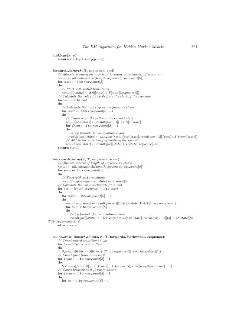
The EM Algorithm for Hidden Markov Models 261
add logs(x, y):return x + log(1 + exp(y − x))
forwards array(S, T, sequence, end):// Allocate memory for matrix of forwards probabilities, of size n × lresult← allocate matrix(length[sequence], row count[S])for state← 1 to row count[S]do
// Start with initial transitionsresult[0][state]← S[0][state] + T [state][sequence[0]]
// Calculate the value forwards from the start of the sequencefor pos← 0 to enddo
// Calculate the next step in the forwards chainfor state← 1 to row count[S] − 1do
// Traverse all the paths to the current stateresult[pos][state]← result[pos− 1][1] + S[1][state]for from← 2 to row count[S] − 1do
// log formula for summation chainsresult[pos][state]← add logs(result[pos][state], result[pos−1][from]+S[from][state])
// Add in the probability of emitting the symbolresult[pos][state]← result[pos][state] + T [state][sequence[pos]]
return result
backwards array(S, T, sequence, start):// Allocate matrix of length of sequence vs statesresult← allocate matrix(length[sequence], row count[S])for state← 1 to row count[S]do
// Start with end transitionsresult[length[sequence]][state] ← S[state][0]
// Calculate the value backwards from endfor pos← length[sequence] − 1 to startdo
for state← 1torow count[S] − 1do
result[pos][state]← result[pos + 1][1] + (S[state][1] + T [1][sequence[pos]])for to← 2 to row count[S] − 1do
// log formula for summation chainsresult[pos][state] ← add logs(result[pos][state], result[pos + 1][to] + (S[state][to] +
T [to][sequence[pos]]))return result
count transitions(S counts, S, T, forwards, backwards, sequence):// Count initial transitions 0-¿nfor to← 1 to row count[S] − 1do
S counts[0][to]← S[0][to] + (T [to][sequence[0]] + backwards[to][1])// Count final transitions n-¿0for from← 1 to row count[S] − 1do
S counts[from][0]← S[from][0] + forwards[from][length[sequence] − 1]// Count transitions k-¿l where k,l!=0for from← 1 to row count[S] − 1do
for to← 1 to row count[S]− 1

262 I. B. Hallgrımsdottir, R. A. Milowski and J. Yu
doS counts[from][to]← forwards[from][0]+(S[from][to]+(T [to][sequence[1]]+backwards[to][1]))for pos← 1 to length[sequence] − 2do
v ← forwards[from][pos]+(S[from][to]+(T [to][sequence[pos]]+backwards[to][pos+1]))
S counts[from][to]← add logs(S counts[from][to], v)return S counts
count emissions(T counts, T, forwards, backwards, sequence):// Count initial transitions 0-¿nfor state← 1 to row count[S] − 1do
T counts[state][sequence[0]] ← forwards[state][0] + backwards[state][0]for state← 1 to row count[S] − 1do
for pos← 1 to length[sequence] − 1do
T counts[state][sequence[pos]] ← add logs(T counts[state][sequence[pos]], forwards[state][pos]+backwards[state][pos])
return T counts
Baum Welch(S, T, sequences, limit):lastLogLikelihood ← −∞repeat
logLikelihood ← 0// These are matricesS counts ← zero matrix(S)new S ← zero matrix(S)T counts ← zero matrix(T )new T ← zero matrix(T )for s← 0 to length[sequences] − 1do
sequence ← sequences[s]// Get the forwards/backwards values for the current sequence & model parametersforwards← forwards array(S,T, sequence, length[sequence] − 1)backwards ← backwards array(S,T, sequence, 0)// Calculate sequence probabilityseqprob← forwards[1][length[sequence]] + S[1][0]for state← 2 to row count[S] − 1do
seqprob← add logs(seqprob, forwards[state][length[sequence]] + S[state][0])// Add contribution to log-likelihoodlogLikelihood ← logLikelihood + seqprob// Calculate the ”counts” for this sequenceS counts ← count transitions(S counts, S, T, forwards, backwards, sequence)T counts ← count emissions(T counts, T, forwards, backwards, sequence)// Calculate contribution for this sequence to the transitionsfor from← 0 to row count[S] − 1do
for to← 1 to row count[S]− 1do
if s = 0then
new S[from][to]← S counts[from][to]− seqprobelse
new S[from][to]← add logs(new S[from][to], S counts[from][to]− seqprob)// Calculate contribution for this sequence to the transitionsfor sym ← 0 to row count[T ]− 1do
if s = 0

The EM Algorithm for Hidden Markov Models 263
thennew T [from][sym]← T counts[from][sym] − seqprob
elsenew T [from][sym]← add logs(new T [from][sym], T counts[from][sym]−seqprob)
// We’ll stop when the log-likelihood changes a small amountchange ← logLikelihood − lastLogLikelihood
until change < limitreturn S, T
12.2 Evaluating the likelihood function
The likelihood function for a hidden Markov model is
Lobs =∏
τ∈(Σ′)n
fτ (θ, θ′)uτ .
Hence Lobs is a polynomial of degreeNn(n−1) whose variables are the unknown
parameters in the matrices θ and θ′. It is in general not possible to obtain the
MLEs, θ and θ′, directly, so the Baum-Welch algorithm is used. However,
for short Markov chains with few states and output variables it is possible
to obtain the MLEs directly. We will look at a few examples of likelihood
functions that arise from two state HMMs of length 3 with binary output (so
l = 2, n = 3, l′ = 2). If we fix the initial probabilities at 0.5 the model has
4 free parameters. For simplicity, we will denote the transition and emission
probabilities by
θ =
(x 1− x
1 − y y
)and θ′ =
(z 1 − z
1 −w w
).
For a fixed set of observed data, the likelihood function Lobs is a polynomial
in the variables x, y, z, and w. We are interested in maximizing Lobs over the
region 0 ≤ x, y, z, w ≤ 1. More generally, we want to study how many critical
points Lobs typically has. We make the following observation; Lobs(x, y, 0.5, 0.5)
is constant with respect to x and y and also Lobs(x, y, z, w) = Lobs(y, x, 1 −w, 1− z) for any x, y, z, w. Therefore the critical points and global maxima of
Lobs occur in pairs for the four parameter model.
In the rest of this section, we will look at the likelihood functions for the
six examples listed in the following table. In each example we either fix one
or two of the emission probabilities or impose symmetry constraints on the
transition probabilities, thereby reducing the number of free parameters to 2
or 3 and allowing visualization in 3 dimensions. For each model a data vector

264 I. B. Hallgrımsdottir, R. A. Milowski and J. Yu
uτ is given.
000 001 010 011 100 101 110 111 N z w
Example 1 113 102 80 59 53 32 28 33 500 12/17 12/17
Example 2 26 31 44 4 9 16 40 35 205 12/17 12/17
Example 3 37 20 35 46 29 13 50 33 263 0.635 0.635
Example 4 73 56 49 51 70 53 67 81 500 free 0.1
Example 5 116 88 67 85 51 37 31 25 500 z = w z = w
Example 6 37 20 35 46 29 13 50 33 263 z = w z = w
In the first three examples we specialize z and w to a constant, so there are
only two free parameters, x and y. Using a Singular implementation, by Luis
Garcia, of the algebraic method for obtaining maximum likelihood estimates
described in Section 3.3, we find that the likelihood function in the first example
has a single critical point (0.68838697, 0.33743958), which is a local and global
maximum.
We can plot the likelihood as a function of x and y using MATHEMAT-
ICA, which was introduced in Chapter 2. For simplicity and better precision,
we use 1 instead of 0.5 for the initial probabilities. This only scales the like-
lihood function by a constant and does not change the critical points. The
MATHEMATICA code is:
s[0,0] := x; s[0,1] := 1-x; s[1,0] := 1-y; s[1,1] := y;t[0,0] := 12/17; t[0,1] := 5/17; t[1,0] := 5/17; t[1,1] := 12/17;f[i_,j_,k_]:=Sum[t[a,i]*Sum[s[a,b]*t[b,j]*Sum[s[b,c]*t[c,k],c,0,1],b,0,1],a,0,1];L := Product[Product[Product[f[i,j,k]^u[i,j,k], k,0,1], j,0,1], i,0,1];u[0,0,0] = 113; u[0,0,1] = 102; u[0,1,0] = 80; u[0,1,1] = 59;u[1,0,0] = 53; u[1,0,1] = 32; u[1,1,0] = 28; u[1,1,1] = 33;Plot3D[L,x,0,1, y,0,1, PlotPoints -> 60, PlotRange -> All];
The resulting plot can be viewed in the first panel of Figure 12.1. This is a
typical likelihood function for this model. In fact we randomly generated sev-
eral hundred data vectors uτ and for each of them we examined the likelihood
as a function of x and y for various values of z = w. There was almost always
only one local maxima. We did find a handful of more interesting examples,
including the ones in Example 2 and Example 3. The following code was used
to generate the data in MATHEMATICA:
<< Graphics‘Animation‘s[0, 0] := x; s[0, 1] := 1-x; s[1, 0] := 1-y; s[1, 1] := y;t[0, 0] := z; t[0, 1] := 1-z; t[1, 0] := 1-z; t[1, 1] := z;f[i_,j_,k_]:=Sum[t[a,i]*Sum[s[a,b]*t[b,j]*Sum[s[b,c]*t[c,k],c,0,1],b,0,1],a,0,1];L := Product[Product[Product[f[i, j, k]^u[i, j, k], k, 0, 1], j, 0, 1], i, 0, 1];For[n = 1, n <= 3, n++,
u[0, 0, 0] = Random[Integer, 1, 50]; u[0, 0, 1] = Random[Integer, 1, 50];u[0, 1, 0] = Random[Integer, 1, 50]; u[0, 1, 1] = Random[Integer, 1, 50];u[1, 0, 0] = Random[Integer, 1, 50]; u[1, 0, 1] = Random[Integer, 1, 50];u[1, 1, 0] = Random[Integer, 1, 50]; u[1, 1, 1] = Random[Integer, 1, 50];Print[u[0, 0, 0], ",", u[0, 0, 1], ",", u[0, 1, 0], ",",u[0, 1, 1], ",",u[1, 0, 0], ",", u[1, 0, 1], ",", u[1, 1, 0], ",", u[1, 1, 1]];

The EM Algorithm for Hidden Markov Models 265
MoviePlot3D[L, x, 0, 1,y, 0, 1, z, 0, 1, PlotPoints -> 40, PlotRange -> All]]
We obtained the critical points for the likelihood functions as before. For
Example 2 there are three critical points in the unit square 0 ≤ x, y ≤ 1, namely
a local and global maximum at (0.13511114, 0.31536773), a local maximum at
(0.7828824, 0.72776217), and a saddle point at (0.61297887, 0.61172163). In
Example 3, the unique global maximum occurs on the boundary of the unit
square but there is also a local maximum at (0.65116323, 0.7092192) and a
saddle point at (0.27783904, 0.55326519). In section 12.3 we will return to
these three examples.
In Examples 4-6 we look at models with three free parameters. It is no
longer possible to obtain the critical values analytically as before, and we can-
not plot a function in three variables. However we can look at level surfaces (3
dimensional contours) of the log-likelihood. For example, the following MATH-
EMATICA code can be used to plot the level surface of the log-likelihood
function in Example 6 at the value −363.5.
<< Graphics‘ContourPlot3D‘s[0, 0] := x; s[0, 1] := 1 - x; s[1, 0] := 1 - y; s[1, 1] := y;t[0, 0] := z; t[0, 1] := 1 - z; t[1, 0] := 1 - z; t[1, 1] := z;f[i_,j_,k_]:=Sum[t[a,i]*Sum[s[a,b]*t[b,j]*Sum[s[b,c]*t[c,k],c,0,1],b,0,1],a,0,1];logL := Sum[Sum[Sum[u[i, j, k]*Log[f[i, j, k]], k, 0, 1], j, 0, 1], i, 0, 1];u[0, 0, 0] = 37; u[0, 0, 1] = 20; u[0, 1, 0] = 35; u[0, 1, 1] = 46;u[1, 0, 0] = 29; u[1, 0, 1] = 13; u[1, 1, 0] = 50; u[1, 1, 1] = 33;ContourPlot3D[logL, x, 0.01, 0.99, y, 0.01, 0.99, z, 0.01, 0.99,
Contours -> -363.5, PlotPoints -> 10, 6, Axes -> True];
In Example 4, we specialize w to a constant and let z vary. The level sur-
face at −686 can be seen in Figure 12.1. In Examples 5 and 6 we impose
the condition that the emission matrix θ is symmetric, i.e. z = w. The sym-
metry Lobs(x, y, z, w) = Lobs(y, x, 1 − w, 1 − z) then becomes Lobs(x, y, z) =
Lobs(y, x, 1− z). We can estimate the global and local maxima by picking the
log likelihood value using binary search and checking if the corresponding level
surface is empty. A weakness of this method is that sometimes MATHEMAT-
ICA mistakenly outputs an empty level surface if the resolution is not high
enough. For Example 5 and 6, the level surfaces gets closer to the boundaries
z = w = 0 and z = w = 1 as we gradually increase the likelihood value.
Hence there seem to be two global maxima on the boundaries z = w = 0 and
z = w = 1 in each example. In Example 6, there are also two local maxima
on the boundaries x = 0 and y = 0. Example 3 has the same data vector as
Example 6, so it is a ”slice” of Example 6.
We did not find any examples where there are local maxima inside the
(hyper)cube, but do not know whether that is true in general. For the two
state HMMs with binary output of length 3 and 4, the coordinate functions
f(τ,σ)(θ, θ′) have global maxima on the boundaries z = 0, z = 1, w = 0, w = 1.
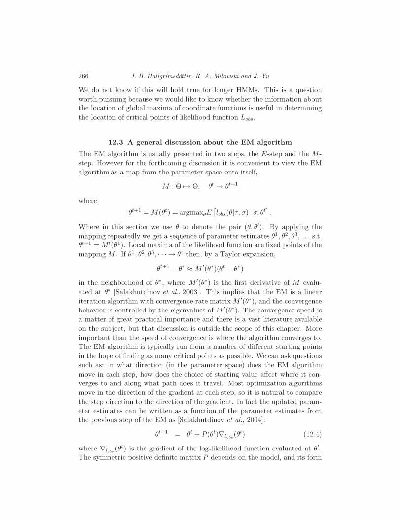
266 I. B. Hallgrımsdottir, R. A. Milowski and J. Yu
We do not know if this will hold true for longer HMMs. This is a question
worth pursuing because we would like to know whether the information about
the location of global maxima of coordinate functions is useful in determining
the location of critical points of likelihood function Lobs.
12.3 A general discussion about the EM algorithm
The EM algorithm is usually presented in two steps, the E-step and the M -
step. However for the forthcoming discussion it is convenient to view the EM
algorithm as a map from the parameter space onto itself,
M : Θ 7→ Θ, θt → θt+1
where
θt+1 = M(θt) = argmaxθE[lobs(θ|τ, σ) | σ, θt
].
Where in this section we use θ to denote the pair (θ, θ′). By applying the
mapping repeatedly we get a sequence of parameter estimates θ1, θ2, θ3, . . . s.t.
θt+1 = M t(θ1). Local maxima of the likelihood function are fixed points of the
mapping M . If θ1, θ2, θ3, · · · → θ∗ then, by a Taylor expansion,
θt+1 − θ∗ ≈M ′(θ∗)(θt − θ∗)
in the neighborhood of θ∗, where M ′(θ∗) is the first derivative of M evalu-
ated at θ∗ [Salakhutdinov et al., 2003]. This implies that the EM is a linear
iteration algorithm with convergence rate matrix M ′(θ∗), and the convergence
behavior is controlled by the eigenvalues of M ′(θ∗). The convergence speed is
a matter of great practical importance and there is a vast literature available
on the subject, but that discussion is outside the scope of this chapter. More
important than the speed of convergence is where the algorithm converges to.
The EM algorithm is typically run from a number of different starting points
in the hope of finding as many critical points as possible. We can ask questions
such as: in what direction (in the parameter space) does the EM algorithm
move in each step, how does the choice of starting value affect where it con-
verges to and along what path does it travel. Most optimization algorithms
move in the direction of the gradient at each step, so it is natural to compare
the step direction to the direction of the gradient. In fact the updated param-
eter estimates can be written as a function of the parameter estimates from
the previous step of the EM as [Salakhutdinov et al., 2004]:
θt+1 = θt + P (θt)∇lobs(θt) (12.4)
where ∇lobs(θt) is the gradient of the log-likelihood function evaluated at θt.
The symmetric positive definite matrix P depends on the model, and its form
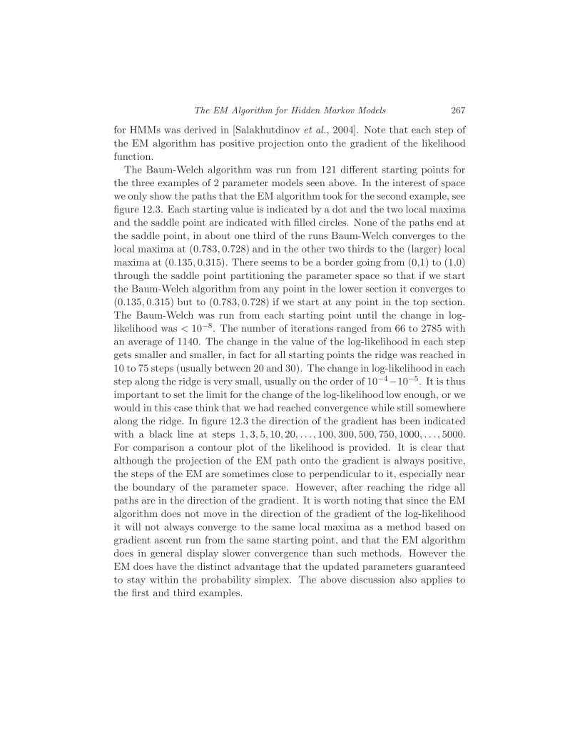
The EM Algorithm for Hidden Markov Models 267
for HMMs was derived in [Salakhutdinov et al., 2004]. Note that each step of
the EM algorithm has positive projection onto the gradient of the likelihood
function.
The Baum-Welch algorithm was run from 121 different starting points for
the three examples of 2 parameter models seen above. In the interest of space
we only show the paths that the EM algorithm took for the second example, see
figure 12.3. Each starting value is indicated by a dot and the two local maxima
and the saddle point are indicated with filled circles. None of the paths end at
the saddle point, in about one third of the runs Baum-Welch converges to the
local maxima at (0.783, 0.728) and in the other two thirds to the (larger) local
maxima at (0.135, 0.315). There seems to be a border going from (0,1) to (1,0)
through the saddle point partitioning the parameter space so that if we start
the Baum-Welch algorithm from any point in the lower section it converges to
(0.135, 0.315) but to (0.783, 0.728) if we start at any point in the top section.
The Baum-Welch was run from each starting point until the change in log-
likelihood was < 10−8. The number of iterations ranged from 66 to 2785 with
an average of 1140. The change in the value of the log-likelihood in each step
gets smaller and smaller, in fact for all starting points the ridge was reached in
10 to 75 steps (usually between 20 and 30). The change in log-likelihood in each
step along the ridge is very small, usually on the order of 10−4−10−5. It is thus
important to set the limit for the change of the log-likelihood low enough, or we
would in this case think that we had reached convergence while still somewhere
along the ridge. In figure 12.3 the direction of the gradient has been indicated
with a black line at steps 1, 3, 5, 10, 20, . . . , 100, 300, 500, 750, 1000, . . . , 5000.
For comparison a contour plot of the likelihood is provided. It is clear that
although the projection of the EM path onto the gradient is always positive,
the steps of the EM are sometimes close to perpendicular to it, especially near
the boundary of the parameter space. However, after reaching the ridge all
paths are in the direction of the gradient. It is worth noting that since the EM
algorithm does not move in the direction of the gradient of the log-likelihood
it will not always converge to the same local maxima as a method based on
gradient ascent run from the same starting point, and that the EM algorithm
does in general display slower convergence than such methods. However the
EM does have the distinct advantage that the updated parameters guaranteed
to stay within the probability simplex. The above discussion also applies to
the first and third examples.
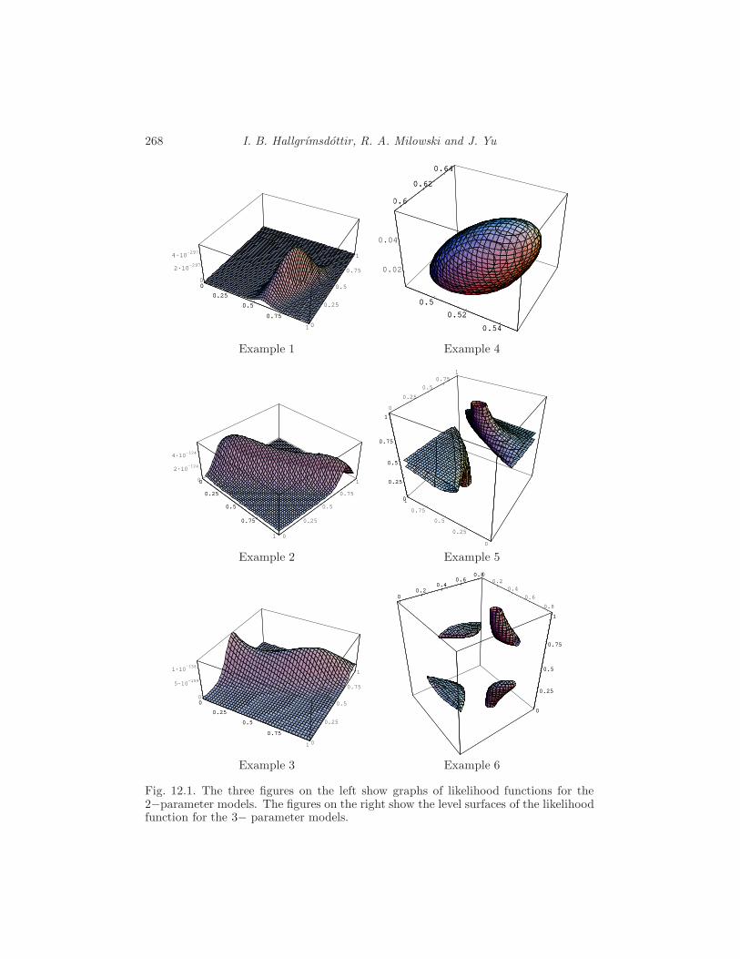
268 I. B. Hallgrımsdottir, R. A. Milowski and J. Yu
0
0.25
0.5
0.75
1 0
0.25
0.5
0.75
1
0
2·10-297
4·10-297
0
0.25
0.5
0.75
0.5
0.52
0.54
0.6
0.62
0.64
0.02
0.04
0.5
0.52
0.54
0.6
0.62
0.64
Example 1 Example 4
0
0.25
0.5
0.75
1 0
0.25
0.5
0.75
10
2·10-124
4·10-124
0
0.25
0.5
0.75
1
0
0.25
0.5
0.751
0
0.25
0.5
0.75
10
0.25
0.5
0.75
1
0
0.25
0.5
0.75
1
Example 2 Example 5
0
0.25
0.5
0.75
1 0
0.25
0.5
0.75
1
0
5·10-159
1·10-158
0
0.25
0.5
0.75
00.2
0.4
0.6
0.8
00.2
0.40.6
0.8
0
0.25
0.5
0.75
1
00.2
0.40.6
0.8
0
0.25
0.5
0.75
1
Example 3 Example 6
Fig. 12.1. The three figures on the left show graphs of likelihood functions for the2−parameter models. The figures on the right show the level surfaces of the likelihoodfunction for the 3− parameter models.
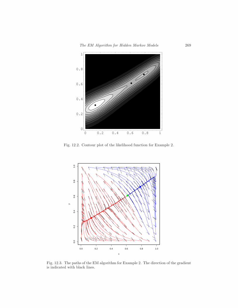
The EM Algorithm for Hidden Markov Models 269
0 0.2 0.4 0.6 0.8 10
0.2
0.4
0.6
0.8
1
Fig. 12.2. Contour plot of the likelihood function for Example 2.
*
*
*
*
*
*
*
*
*
*
*
*
*
*
*
*
*
*
*
*
*
*
*
*
*
*
*
*
*
*
*
*
*
*
*
*
*
*
*
*
*
*
*
*
*
*
*
*
*
*
*
*
*
*
*
*
*
*
*
*
*
*
*
*
*
*
*
*
*
*
*
*
*
*
*
*
*
*
*
*
*
*
*
*
*
*
*
*
*
*
*
*
*
*
*
*
*
*
*
*
*
*
*
*
*
*
*
*
*
*
*
*
*
*
*
*
*
*
*
*
*
0.0 0.2 0.4 0.6 0.8 1.0
0.0
0.2
0.4
0.6
0.8
1.0
x
y
Fig. 12.3. The paths of the EM algorithm for Example 2. The direction of the gradientis indicated with black lines.

13
Homology mapping with Markov Random Fields
Anat Caspi
In this chapter we take a different approach to biological sequence comparison.
We look for portions of the sequences that diverged from the same genomic
region in the closest common ancestor, that is, homologous sequences. We
explore this question as a structured data labelling problem, and offer a toric
model formulation. The exact solution in the general toric model is intractable.
However, for a very relevant subclass of this class of models, we find a linear
(non-integer) formulation that can give us the exact integer solution in polyno-
mial time. This is an encouraging result: for a specific, though widely useful,
subclass of toric models in which the joint probability density is structured,
MAP inference is tractable.
13.1 Genome mapping
Evolution through divergence gives rise to different, though related, present-
day genomes that shared common ancestors. Portions of genomes could also
be seen as genomic entities spawned through some pattern of evolutionary
events from a single entity in the ancestral genome. Such genomic portions
(be they gene-coding regions, conserved non-coding regions, etc) that are re-
lated through divergence from a common region in the ancestral genome are
termed homologs. Homology is therefore a relational term asserting the com-
mon ancestry of two genomic components. Since much of our understanding of
phylogeny and evolution comes from a comparative framework, it is important
to accurately identify those homologous genomic entities in order to compare
components that are actually linked by common ancestry. Additional, more
specific, relational descriptors exist to delineate the evolutionary events that
occurred to initiate the divergence between homologs ; we leave those outside
the scope of this discussion. Our objective is to create a homology mapping :
a mapping between compared sequences in which an element in one sequence
270
Homology mapping with Markov Random Fields 271
mapping to an element in another sequence indicates a homologous relationship
between the two.
Earlier comparative studies aimed to map homology at different levels of res-
olution. At low resolution, gene markers, BAC fingerprints, or chromosomal
locations were used to map entire genes on long genomic regions like chro-
mosomes. At high resolution, nucleotide sequence mapping was designed for
the available genomic sequences: usually short regions coding for one or two
genes. Alignment models such as those discussed in chapter 7 were introduced
. Note that the pair hidden Markov model introduced assumed collinearity
(i.e., that the sequences compared can be mapped sequentially). This was a
result of adopting local alignment models to align relatively short sequences.
This model design primarily intended to deal with point mutations, rather
than large-scale mutations (like gene inversions, or chromosomal duplication)
which are more likely to be found in longer sequences. Assuming collinearity
places an ordering constraint on the mapping produced.
As entire genome sequences are available, we are interested in mapping
longer sequence regions, and must offer a model that does not imbed the or-
dering constraint. However, biological evidence (see [Marcotte et al., 1999],
[P. and G., 2003]) suggests that as genomes diverge, functional constraints ap-
ply pressure against genome shuffling, inversions, and duplications. As a result,
homologs are more likely to occur in sequential syntenic clumps in the genome.
That is, although we shouldn’t constrain our maps to be ordered, we should
look at genomic context and prefer locally collinear homologs. The model sug-
gested here expresses dependencies among locally interacting portions of the
genome, thereby having an affinity towards locally collinear alignments, but
allows mappings that contain rearrangements like duplications and inversions.
The suggested output is a mapping between the genomic sequences that
is not constrained to preserve the order of the sequences if the most likely
mapping contains a rearrangement. Additionally, the mapping may not be
one-to-one: a single component in one sequence may be mapped non-uniquely
to several components in a second sequence, indicating a genomic duplication
event. Due to these differences from the traditional meaning of a sequence
alignment, we use the term homology mapping to describe the desired output.
We can pose the homology mapping problem as a graph assignment prob-
lem. Let us consider a homolog pair as a single entity, representing a single
divergence occurrence from a particular component in an ancestral sequence.
We call a proposed homolog pair a match– a match i, postulates homology
between component a in one sequence, a ∈ S1, with component b in another
sequence, b ∈ S2. The components, a and b, matched by a match need not
be atomic subunits of the sequence (such as a single base-pair), matches could
272 A. Caspi
be proposed between regions of genomic sequences, or even entire structural
domains.
Given genomic sequences for comparison, we introduce a graph in which
proposed homolog pairs (matches) are nodes. We represent the local context
dependencies among matches in our graph by introducing edges among match
nodes whose components are located within a specified base-pair distance in
the genomic sequence of at least one of the two paired components. This
introduces a notion of locality of a node in the graph- where locality denotes
a neighborhood of genome location.
We can choose to attribute weights to the dependencies among the matches.
Edge weights can quantify associations among matches based on proximity
or genomic distance, match density, orientation, or whether considering both
matches homologs would necessitate particular genomic events (like inversions,
duplications or shuffling) in their divergence pattern. Our objective is to choose
a graph coloring for all the nodes in such a way that the sum of the weights
on the edges connecting like-colored nodes is minimized. A discrete binary
coloring scheme (for example, black and white) is natural to this problem
since there are no partial homologs– components either did (black) or did not
(white) share a common ancestor.
We are interested in solving this discrete labelling task probabilistically.
Assuming a common ancestor between two sequences, we treat evolutionary
events as part of a stochastic biological process that results in many pairs of
homologous diverged genomic components that are distributed according to
stochastically defined local spatial relations. To summarize: the model ought
to capture context-dependent interactions among locally-interacting objects in
a probabilistic manner. This is a an instance of a structured labelling problem.
Markov random fields (MRF) are a stochastic approach to modelling struc-
tured labelling problems. In MRFs, the label class (in our case homolog/non-
homolog) pattern is generated by a random process. The parameters of the
process induce the particular configuration of the correct labelling of the nodes.
The random processes modelled by MRFs provide properties of local depen-
dencies whereby the probability of a specific label (in our case, the probability
that a match is or is not a homolog) is entirely dependent on a local subset of
neighboring labels (in our case, a match is dependent on its immediate genomic
context).
13.2 Markov random fields
Our goal here is to introduce the log-linear Markov Random Field model us-
ing algebraic notation (for a more general exposition of MRFs in algebraic
statistics refer to [Geiger et al., 2002]). The model consists of an underlying

Homology mapping with Markov Random Fields 273
topology specified by an undirected graph G ≡ (Y, E) (like the one introduced
in example 1.), and a strictly positive probability distribution which factors
according to the graph. Y = Y1, . . . , YN contains N nodes representing ran-
dom variables. A node i has an assignment σi from a finite alphabet Σi of
li = |Σi| values or states. For example, if our nodes are binary random vari-
ables (for instance, indicating not homolog or homolog), then ΣY = 0, 1, as
there are two possible values for each node factors, and |ΣY| = lY = 2. The
state space is the finite and enumerable product space of all possible assign-
ments Y =∏
Yi∈YΣYi . In the case of a uniform alphabet of size lY for all the
nodes in the graph, this state space comprises of m = |ΣY|N = lNY possible
assignments.
We turn our attention to the set of edges in the graph. E is a subset of Y×Y.
Each edge, denoted eij, is an undirected edge between nodes i and j in Y.
The edges define neighborhood associations in the form of direct dependencies
among nodes. We define the neighborhood of node i as the set of all nodes j
to which i is connected by an edge, Ni = j | i, j ∈ Y, i 6= j, ei,j ∈ E. The
neighborhood of i is sometimes referred to as the Markov blanket of i. While
Markov blankets describe the web of associations for a particular node, the
entire graph could be factorized into subsets of maximally connected subgraphs
in G, known as cliques. Cliques vary in size. The set of cliques of size one,
C(G)1 = i | i ∈ Y, Ni = ∅ is a subset of the nodes in the graph; the set of
cliques of size two is a subset of the adjacent nodes (or pair-matches), C(G)2 =
(i, j) | j ∈ Ni, i ∈ Y; the set of cliques of size three enumerates triples of
neighboring nodes, C(G)3 = (i, j, k) | i, j, k ∈ Y, eij, ejk, eik ∈ E, etc. The
collection of all cliques in the graph is C(G) = C(G)1⋃ C(G)2
⋃C(G)3⋃ · · ·.
C(G) induces a decomposition of the graph into factors. Decomposing a graph
in this way is instrumental both in understanding dependencies among the
nodes, and in performing efficient inference as will be described below.
Each clique factor of a general Markov random field has a potential function
which associates a non-negative value with each possible assignment of the
nodes in that clique. In the log-linear class of models, the positivity constraint
is imposed on the probability density function which in turn restricts the poten-
tial functions to be strictly positive. This restriction is enforced by expressing
the potential valued functions in the exponential family form e(T (σ)), where
T (σ) is the sufficient statistic for the family. We denote the potential value
of a particular instance of a clique by φci(σci), where σci is an instantiation
of all the nodes in clique ci. In the discrete case, the potential function for
each clique ci ∈ C(G) could be represented by a contingency matrix, θci , of k
dimensions (where k is the [size of the clique vs. cardinality of ci], |ci| = k).
θci is indexed by a k-tuple, (σ1, σ2, . . .σk) where σj ∈ Σj, the finite alphabet
from which node j ∈ ci takes its value. This contingency matrix associates
274 A. Caspi
a positive value with each possible assignment for all nodes in the clique. As
noted, positive valued potential functions induce strict positivity on the distri-
butions generated by the cliques. Positivity is one of the two main properties
of the random processes that log-linear MRFs model, and is a requirement of
the Hamemrsley-Clifford theorem.
The random processes addressed by all MRFs preserve the Markov property.
Specifically, as noted above, each edge association is a conditional independence
statement which the probability distribution must satisfy. (Let σi denote the
state (or: a particular assignment) for the node i ∈ Y.)
P(σi|σY\i) = P(σi|σNi) (13.1)
The Markov property states that the probability of a particular labelling for
node i (given the rest of the labelled graph nodes) is only conditioned on the
local Markov blanket of node i. That is, to assess a node’s conditional prob-
ability, we only need the specification of its local neighborhood. Additionally,
we see that two nodes, i and j, that do not share an edge in E must be
conditionally independent because their Markov blankets are disjoint,
P(σi, σj|σY\i,j) = P(σi|σNi)P(σj|σNj) ∀i, j | eijBy definition, every node j not in the Markov blanket of i is conditionally
independent of i given the other nodes in the graph:
i ⊥⊥ j |Y\i, j ∀j * Ni, i, j ∈ Y
Note that the set of Markov statements applied to each node i ∈ Y, is the
full set of conditional independence statements MG (previously introduced in
(1.63)) necessary and sufficient to specify the undirected graphical model in
its quadratic form.
When the individual node probabilities and their Markov blankets are put
together, the graph factorizes as the maximally connected subgraphs in the
graph, introduced above as C(G). In this class of models, specifying the factor-
ization and the potential function for each factor is tantamount to specifying
the joint probability distribution of all variables for the Markov random field.
Specifically, the log linear probability distribution on a full assignment to the
graph labels, σ, is defined as:
P (σ) =1
Z
∏
ci∈C(G)
φci(σci)
where Z is the partition function given by Z =∑
σ∈Σn
∏ci∈C(G)
φci(σci).
The probability is only dependent on the exponential family potential func-
tions, and the node assignments in σ. We can therefore equivalently param-
eterize the model by the collection of contingency matrices, θci , one for each
Homology mapping with Markov Random Fields 275
maximally connected subgraph, ci ∈ C(G). The probability distribution over
the state space is then defined to be proportional to the product of the param-
eters relevant to the particular model instantiation,
Pθ(σ) ∝∏
ci∈C(G)
θci
σ′ci
I(σ′
ci≡ σci) (13.2)
where I(·) is the boolean indicator function. The proportionality constant is
the partition function as above. The components of θ are enumerable. For
instance, in a Markov random field whose nodes take value assignments from
the same alphabet, Σ such that |Σ| = l, the number of (potential values vs.
potential valued functions) in the graph is
d =∑
ci∈C(G)
l|ci|·
We call the cliques in the factorized graph C(G) the model generators, defining
d unknown, positive, model parameters θ = θ1, . . . , θd.We have characterized a class of undirected graphical models which is log-
linear in the parameter values. Given the finite state space Σn, we can define
an associated monomial mapping in θ for each assignment σ ∈ Σn.
fσ(θ) = Pθ(σ) =1
Z
d∏
j=1
θjI(j ∈ σ)
Recall that θ is indexed by a generator and its possible instantiation. Hence,
the degree of each θj is determined by the state of the associated factors in
the assignment. Since every factor must take on one and only one state label,
the degree of all m monomials associated with a valid assignment is the same.
Pooling all such monomials into a single map f , we have specified a toric model
parametrically (for definition of a toric model see 1.26).
f : Rd → Rm , θ 7→ 1∑mj=1 fj(θ)
·(f1(θ), f2(θ), . . . , fm(θ)
).
We can express each of the monomials, fi, as a column vector, thereby
constructing a design d ×m integer matrix, A. As before, the toric model of
A is the image of the orthant θ = Rd>0 under the map:
f : Rd → Rm, θ → 1∑mj=1 θ
aj(θa1 , θa2, . . . θam)
where∑m
j=1 θaj is the partition function. By construction, the joint probabil-
ity distribution, P , is in the image of the mapping f , and we say that P factors
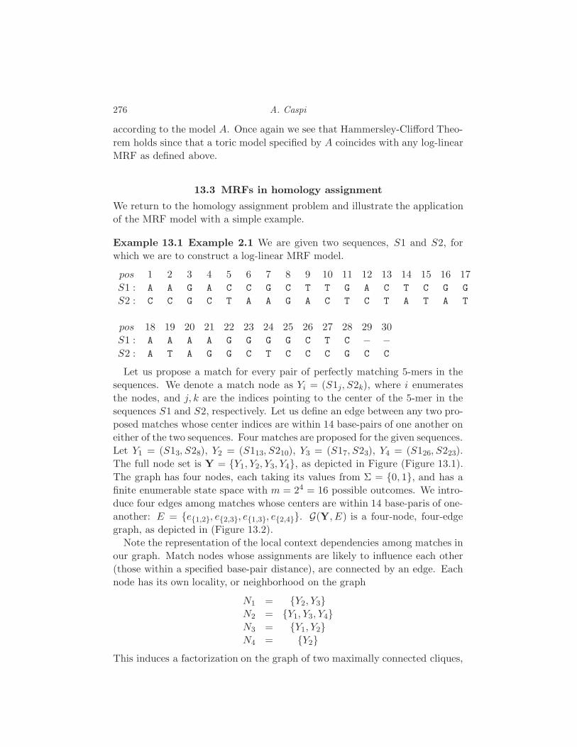
276 A. Caspi
according to the model A. Once again we see that Hammersley-Clifford Theo-
rem holds since that a toric model specified by A coincides with any log-linear
MRF as defined above.
13.3 MRFs in homology assignment
We return to the homology assignment problem and illustrate the application
of the MRF model with a simple example.
Example 13.1 Example 2.1 We are given two sequences, S1 and S2, for
which we are to construct a log-linear MRF model.
pos 1 2 3 4 5 6 7 8 9 10 11 12 13 14 15 16 17
S1 : A A G A C C G C T T G A C T C G G
S2 : C C G C T A A G A C T C T A T A T
pos 18 19 20 21 22 23 24 25 26 27 28 29 30
S1 : A A A A G G G G C T C − −S2 : A T A G G C T C C C G C C
Let us propose a match for every pair of perfectly matching 5-mers in the
sequences. We denote a match node as Yi = (S1j, S2k), where i enumerates
the nodes, and j, k are the indices pointing to the center of the 5-mer in the
sequences S1 and S2, respectively. Let us define an edge between any two pro-
posed matches whose center indices are within 14 base-pairs of one another on
either of the two sequences. Four matches are proposed for the given sequences.
Let Y1 = (S13, S28), Y2 = (S113, S210), Y3 = (S17, S23), Y4 = (S126, S223).
The full node set is Y = Y1, Y2, Y3, Y4, as depicted in Figure (Figure 13.1).
The graph has four nodes, each taking its values from Σ = 0, 1, and has a
finite enumerable state space with m = 24 = 16 possible outcomes. We intro-
duce four edges among matches whose centers are within 14 base-paris of one-
another: E = e1,2, e2,3, e1,3, e2,4. G(Y, E) is a four-node, four-edge
graph, as depicted in (Figure 13.2).
Note the representation of the local context dependencies among matches in
our graph. Match nodes whose assignments are likely to influence each other
(those within a specified base-pair distance), are connected by an edge. Each
node has its own locality, or neighborhood on the graph
N1 = Y2, Y3N2 = Y1, Y3, Y4N3 = Y1, Y2N4 = Y2
This induces a factorization on the graph of two maximally connected cliques,
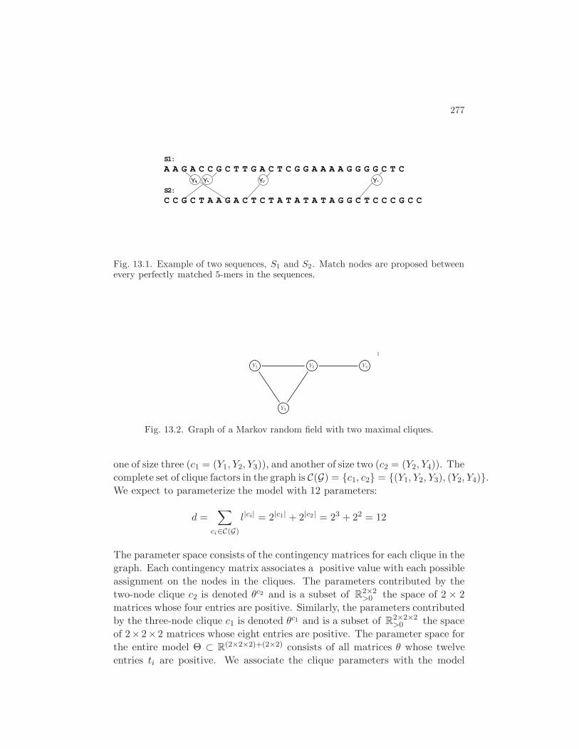
Homology mapping with Markov Random Fields 277
Fig. 13.1. Example of two sequences, S1 and S2. Match nodes are proposed betweenevery perfectly matched 5-mers in the sequences.
1
Y1 Y2 Y4
Y3
Fig. 13.2. Graph of a Markov random field with two maximal cliques.
one of size three (c1 = (Y1, Y2, Y3)), and another of size two (c2 = (Y2, Y4)). The
complete set of clique factors in the graph is C(G) = c1, c2 = (Y1, Y2, Y3), (Y2, Y4).We expect to parameterize the model with 12 parameters:
d =∑
ci∈C(G)
l|ci| = 2|c1| + 2|c2| = 23 + 22 = 12
The parameter space consists of the contingency matrices for each clique in the
graph. Each contingency matrix associates a positive value with each possible
assignment on the nodes in the cliques. The parameters contributed by the
two-node clique c2 is denoted θc2 and is a subset of R2×2>0 the space of 2 × 2
matrices whose four entries are positive. Similarly, the parameters contributed
by the three-node clique c1 is denoted θc1 and is a subset of R2×2×2>0 the space
of 2×2×2 matrices whose eight entries are positive. The parameter space for
the entire model Θ ⊂ R(2×2×2)+(2×2) consists of all matrices θ whose twelve
entries ti are positive. We associate the clique parameters with the model

278 A. Caspi
parameters as follows.
( t1 t2 t3 t4 t5 t6 t7 t8
θc1 = θc1000 θc1
001 θc1010 θc1
011 θc1100 θc1
101 θc1110 θc1
111
)
( t9 t10 t11 t12
θc2 = θc200 θc2
01 θc210 θc2
11
)·
Using this factorization, we can fully characterizes the conditional indepen-
dence relationships among the match nodes. Specifically, we have
P (σ1|σ2, σ3, σ4) = P (σ1|σ2, σ3)
P (σ2|σ1, σ3, σ4) = P (σ2|σ1, σ3, σ4)
P (σ3|σ1, σ2, σ4) = P (σ3|σ1, σ2)
P (σ4|σ1, σ2, σ3) = P (σ4|σ2) ·
There are only 2 pairs of nodes not connected by an edge; the rendered model
is
MG = Y1 ⊥⊥ Y4 | Y2, Y3, Y3 ⊥⊥ Y4 | Y1, Y2, Each such conditional independence statement can be translated into a system
of quadratic polynomials in R[Y]. The representation of independence state-
ments as polynomial equations is an implicit representation of the toric model,
where the common zero set of the polynomials represent the model.
For binary alphabets Σi the following eight quadric forms compose the set
QMGrepresenting the probability distribution from the example above.
p0001p1000 − p0000p1001 , p0001p0010 − p0000p0011 ,
p0011p1010 − p0010p1011 , p0101p0110 − p0100p0111 ,
p0101p1100 − p0100p1101 , p1001p1010 − p1000p1011 ,
p0111p1110 − p0110p1111 , p1101p1110 − p1100p1111.
This set specifies a model which is a subset of the 15-dimensional simplex ∆
with coordinates pσ1σ2σ3σ4. The non-negative points on the variety defined
by this set of polynomials represent probability distributions which satisfy the
conditional independence statements in MG.
The same quadric polynomials can also be determined by the vectors in
the kernel of the parametric matrix d × m model AG . Each quadric form
corresponds to a vector in the kernel of the design matrix AG . The columns
of AG are indexed by the m states in the state space, and the rows represent
the potential values, indexed by a pair consisting of a maximal clique and a
particular assignment possible on that clique, with a separate potential value

Homology mapping with Markov Random Fields 279
for each possible assignment on the clique; 12 parameters in all. Each column
in AG represents a possible assignment of the graph.
0000 0001 0010 0011 0100 0101 0110 0111 1000 1001 1010 1011 1100 1101 1110 1111
000· 1 1 0 0 0 0 0 0 0 0 0 0 0 0 0 0
001· 0 0 1 1 0 0 0 0 0 0 0 0 0 0 0 0
010· 0 0 0 0 1 1 0 0 0 0 0 0 0 0 0 0
011· 0 0 0 0 0 0 1 1 0 0 0 0 0 0 0 0
100· 0 0 0 0 0 0 0 0 1 1 0 0 0 0 0 0
101· 0 0 0 0 0 0 0 0 0 0 1 1 0 0 0 0
110· 0 0 0 0 0 0 0 0 0 0 0 0 1 1 0 0
111· 0 0 0 0 0 0 0 0 0 0 0 0 0 0 1 1
· 0 · 0 1 0 1 0 0 0 0 0 1 0 1 0 0 0 0 0
· 0 · 1 0 1 0 1 0 0 0 0 0 1 0 1 0 0 0 0
· 1 · 0 0 0 0 0 1 0 1 0 0 0 0 0 1 0 1 0
· 1 · 1 0 0 0 0 0 1 0 1 0 0 0 0 0 1 0 1
The geometry of the model is imbedded in this simplex. Each of them columns
of Al,n represents a distinct point in the d-dimensional space. The convex hull
of these points define the polytope fl,n(θ). Referring back to the toric Markov
chain of chapter 1, we saw that the map fl,n was a k dimensional object inside
the (m − 1) dimensional simplex ∆ which consisted of all probability distri-
butions in the state space ln. The dimension k of the polytope is dependent
on the conditionally dependent components, or cliques in the model. In the
modeling literature this is referred to as graph partitions and separators on
the graph.
The equivalence of the expressions of the log-linear Markov distributions
is guaranteed by the important result of the Hammersley-Clifford theorem.
In general, however, without the constraint on strictly positive probability
density functions, px > 0, the class of toric models is larger than the general
MRF exponential model.
13.4 Tractable MAP Inference in a subclass of MRFs
We return to the homology assignment problem. We wished to find the op-
timal factor assignment for Y. In the case we presented, we have a binary
assignment, designating homolog or not homolog. We note that the graph
topology, conditional dependencies among its factors and potential functions
on the graph (the θ vector) were obtained by incorporating observations about
the given biological sequences for which we want homology assignments. In
this case, we are interested in the label assignment to the factors in Y that
280 A. Caspi
maximizes the joint probability of the assignments given the parameter values.
Specifically, we would like to find the mode (peak) of the distribution. This is
called the Maximum A Posteriori (MAP) assignment of the model.
We have already specified the joint probabilities of the assignments Pθ(σ),
given the parameters of the model in 13.2. In terms of the parameters, the
probability of observing σ is the product of the parameters that correspond
to the instantiation of these maximal cliques on the graph normalized by the
partition function. The partition function enumerates (m = |ΣY|N ) possible
assignments, and despite the model factorizing as the graph, calculating the
joint probability is computationally nontrivial. Various mechanisms for esti-
mating the partition function have been suggested. For instance, using Gibbs
distributions, we can obtain a global probability of a labelling by sampling
from the distribution ([Geman and Geman, 1984]). We’re interested in an ex-
act MAP solution that is tractable. Tractable MAP computation is possible
for a specific subclass of toric models which is very relevant to the homology
assignment problem and other discrete labelling problems.
First, let us try to simplify the MAP inference computation. We transform
the problem to logarithmic coordinates log(Θ), where the joint probability
density calculation for every assignment becomes a linear sum:
log(Pθ(σ)) =∑
ci∈C(G)
θci
σ′ci
I(σ′
ci≡ σci)− log(Z)
This is the polytope calculated from the m columns of matrix − log(AG). Com-
puting a vertex on the convex hull of this matrix is the same as tropicalizing
the partition function. This reduces the problem to calculating the convex
hull of − log(Pθ(σ)) and finding the maximal vertex. Evaluating the partition
function is intractable beyond small sized problems because the computation
is exponential in the number of nodes on the graph (for a more detailed dis-
cussion, see chapter 9). This makes computation of the entire joint probability
very difficult. There exists a subclass of log-linear models for which MAP in-
ference can be computed exactly by reformulating the problem as a problem
for which we already have efficient algorithms.
For many integer and combinatorial optimization problem, some very suc-
cessful approximation algorithms are based on linear relaxations, such as branch-
and-cut. In general, these are approximation algorithms. However, for a cer-
tain subclass of the log-linear models called ferromagnetic Ising models, solving
the integer programming problem based on a linear relaxation gives an exact
solution to the problem [Besag, 1986, Kolmogorov and Zabih, 2003]. This sub-
class encodes situations in which locally related variables (nodes in the same
Markov blanket) tend to have the same labelling. In this subclass, the contin-
gency matrix for each generator of the model (maximal clique) is constrained

Homology mapping with Markov Random Fields 281
to have all of the off-diagonal terms be identically one, and all the diagonal
terms be greater than one. When we take the logarithm of these terms, the
off-diagonal terms vanish, and the diagonal terms are strictly positive. Those
familiar with computer vision or physics literature would recognize this is akin
to the generalized Potts, but with no penalty for assignments that do not have
the same label across edges in the graph.
Recall that the diagonal terms are those which assign the same label to all
the nodes in the same maximal clique. This type of value assignment is known
as guilt by association, since being in the same clique (local neighborhood) has a
positive potential value (hence increasing the likelihood) associated with being
assigned the same value. In the context of the homology assignment, this is a
way of representing an underlying evolutionary process in which homologous
matches are related objects whose homology assignment should be consistent
with other local matches. This kind of attractive assignment is important
in many domains in which different labels have structures of affinities within
local neighborhoods. In our formulation, the different labels can have different
affinities.
To formulate the linear relaxation for solving this problem, we must leave the
realm of toric varieties. The state space now comprises of continuous vectors.
In the implicitization of the model, we maintain the quadric polynomials we
had before (that is, the conditional independence statements remain the same).
We present new polynomials that ensure that a particular value assignment,
(σci) = k, on a clique is only possible when all the component nodes j ∈ ciare assigned the same value, k. The new model is represented by the non-
negative set of the added quadric polynomials (a set of inequalities) rather than
the common zero set of all the polynomials as before. These new constraints
did not add points to the model outside the convex hull of the original toric
model. Hence, the polytope remains the same, only the linear formulation
incorporates more than just the integer lattice vertices in the set of feasible
solutions. Importantly, it has been shown that in the binary case, when a
solution exists, the linear relaxation is guaranteed to produce the same integer
solution as the integer model [Besag, 1986, Kolmogorov and Zabih, 2003]. In
practice, this problem conveniently reduces to a problem known as graph min-
cut, which can be solved exactly in polynomial time only in the number of
nodes on the graph.
This is an encouraging result: for a specific, though widely applicable, sub-
class of toric models in which the joint probability density is structured, MAP
inference is tractable.

282 A. Caspi
13.5 The Cystic Fibrosis Transmembrane Regulator
The ’greater Cystic Fibrosis Transmembrane Regulator (CFTR) region’ is a
DNA dataset of 12 megabases (Mb) of high-quality sequences from 12 verte-
brate genomes. The data was collected by Thomas et. al. [Thomas et al., 2003],
targeting a genomic region orthologous to a segment of about 1.8 Mb on hu-
man chromosome 7, which encodes 10 genes. One of the genes encodes CFTR,
which is the gene mutated in cystic fibrosis.
The original comparative study successfully identified 98% of the exons as
well as many conserved noncoding sequences. The gene number and order were
found to be mostly conserved across the 12 species, with strikingly variable
amount of noncoding sequences mainly interspersed repeats. Additionally,
the authors identified three insertions (transposons) that are shared between
the primates and rodents, which confirms the close relationship of the two
lineages and highlights the opportunity such data provides for refining species
phylogenies and characterizing the evolutionary process of genomes.
To demonstrate the use of our method, we took the greater CFTR region
from four currently sequenced vertebrate genomes: human, chicken, rat and
mouse.
In practice, our method delineates the sequence matching (see chapter 7)
from the homology mapping aspects of alignment. To produce homolog map-
pings among multiple sequences, we proceed as follows:
(i) Obtain matches (not necessarily identical) between multiple sequences
in advance of the homology mapping: these matches may be pairs of
single base pairs, larger BLAT hits[Kent, 2002], exons, or even complete
genes.
(ii) Construct the constrained Ising model based on the matches (as above).
(iii) Find the MAP assignment using linear programming.
(iv) Output the nodes that were assigned a value of 1 as homologous matches.
Figure 13.3 displays the CFTR dataset for the four selected genomes. Hor-
izontal shaded bars represent the CFTR region in a fully sequenced chromo-
some. The lines between chromosome bars connecting small segments represent
BLAT[Kent, 2002] output matches.
Our method takes these matches as nodes, and constructs a Markov network
from them. In this particular instance, there are 169 nodes and our network
has nearly six thousand edges. On a (machine spec here) it took 12.18 seconds
to solve the corresponding linear program formulation. The results (that is,
the nodes that were assigned a value of 1, designated as homolog) are depicted
in figure 13.4.
Overall, we have performed this operation on much larger sets of data, with
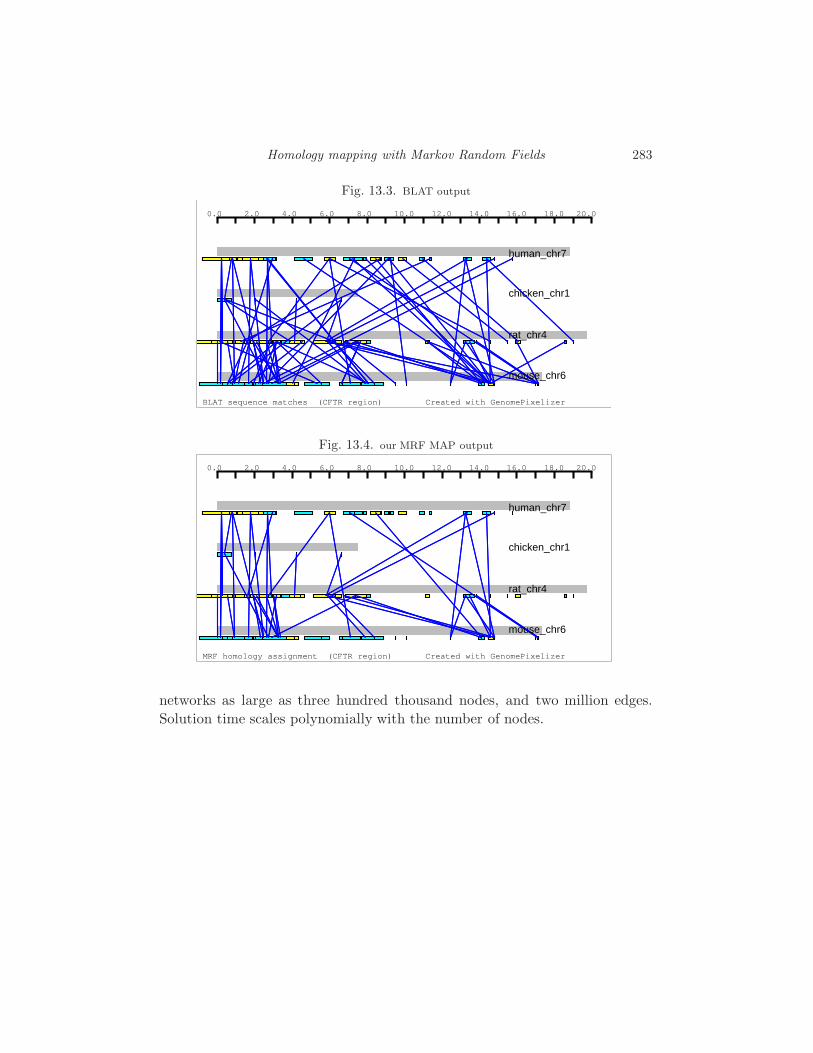
Homology mapping with Markov Random Fields 283
Fig. 13.3. BLAT output
BLAT sequence matches (CFTR region) Created with GenomePixelizer
0.0 2.0 4.0 6.0 8.0 10.0 12.0 14.0 16.0 18.0 20.0
human_chr7
chicken_chr1
rat_chr4
mouse_chr6
Fig. 13.4. our MRF MAP output
MRF homology assignment (CFTR region) Created with GenomePixelizer
0.0 2.0 4.0 6.0 8.0 10.0 12.0 14.0 16.0 18.0 20.0
human_chr7
chicken_chr1
rat_chr4
mouse_chr6
networks as large as three hundred thousand nodes, and two million edges.
Solution time scales polynomially with the number of nodes.
14
Mutagenetic Tree Models
Niko Beerenwinkel
Mathias Drton
Mutagenetic trees are a class of graphical models designed for accumulative
evolutionary processes. We determine the algebraic invariants of mutagenetic
trees and discuss the geometry of mixture models.
14.1 Accumulative Evolutionary Processes
Some evolutionary processes can be described as the accumulation of non-
reversible genetic changes. For example, the progression of tumor development
of several cancer types can be regarded as the accumulation of chromoso-
mal alterations [Vogelstein et al., 1988, Zang, 2001]. This clonal evolutionary
process starts from the set of complete chromosomes and is characterized by
subsequent chromosomal gains and losses or by losses of heterozygosity. Muta-
genetic trees (also called oncogenetic trees in the context of oncogenesis) have
been applied to model the occurrence of chromosome alterations in patients
with renal cancer [Desper et al., 1999, von Heydebreck et al., 2004], ovarian
adenocarcinoma [Simon et al., 2000], and melanoma [Radmacher et al., 2001].
For glioblastoma and prostate cancer, tumor progression along the oncogenetic
tree model has been shown to be an independent marker of patient survival
[Rahnenfuhrer et al., 2005].
Amino acid substitutions may also be modeled as permanent under certain
conditions, such as a very strong selective pressure. For example, the evolution
of human immunodeficiency virus (HIV) under antiviral drug therapy exhibits
this behavior. The development of drug resistance can be regarded as the ac-
cumulation of resistance-conferring mutations. Mixtures of mutagenetic trees
have been applied to data sets obtained from HIV infected patients under differ-
ent antiviral drug regimens [Beerenwinkel et al., 2004, Beerenwinkel et al., 2005a].
This modeling approach has revealed different evolutionary pathways the virus
can take to become resistant, which is important for the design of effective
therapeutic protocols.
284
Mutagenetic Tree Models 285
In general, we consider clonal evolutionary processes on a finite set of events.
An event can be a genetic alteration, such as the loss of a chromosome arm in
a tumor cell or an amino acid substitution in a protein. We assume that
these changes are permanent. Mutagenetic trees aim at modeling the or-
der and rate of occurrence of these changes. A software package for statis-
tical inference with mutagenetic trees and mixtures of these is described in
[Beerenwinkel et al., 2005b].
14.2 Mutagenetic Trees
Consider n binary random variables X1, . . . , Xn each indicating the occurrence
of an event. We will represent an observation of X := (X1, . . . , Xn) as a
binary vector i = (i1, . . . , in) ∈ I := 0, 1n, but sometimes use the equivalent
representation by the subset Si ⊂ [n] = 1, . . . , n of occurred events, i.e.
Si = v ∈ [n] | iv = 1. The inverse of this bijection is simply iS = (1S, 0V \S).
For a subset A ⊂ [n] we denote by XA = (Xv)v∈A the correponding subvector
of random variables taking values in IA := 0, 1|A|.A mutagenetic tree T on n events is a connected branching on the set of nodes
V = V (T ) = 0 ∪ [n], rooted at node 0. The set of edges in T is denoted by
E(T ). There are (n+1)n−1 different mutagentic trees on n events. Indeed, the
set of connected rooted branchings on V is in one-to-one correspondence with
the set of undirected labeled trees on n+1 nodes, and Cayley’s theorem states
that this set has cardinality (n+1)n−1 [Stanley, 1999]. A subbranching of T is
a directed subtree of T with the same root node 0. For any subset V ′ ⊂ V we
denote by TV ′ the induced subgraph. In particular, each state i ∈ I induces a
subgraph Ti := TSi of the mutagenetic tree T . Every node v ∈ [n] has exactly
one entering edge (u, v) ∈ E(T ). We call u the parent of v, denoted pa(v) = u.
For V ′ ⊂ V , pa(V ′) is the vector (pa(v))v∈V ′ . Finally, the outgoing edges of a
node u are called the children of u, and this set is denoted ch(u).
For n = 3 events, there are 42 = 16 mutagenetic trees, which fall into
four distinct groups according to the tree topology. Figure 14.1 shows one
mutagenetic tree from each of the four topology classes.
14.2.1 Statistical Model
With each edge (pa(v), v), v ∈ [n], in a mutagenetic tree T , associate a proba-
bility θv11 ∈ [0, 1] and a matrix
θv = θpa(v),v =
(1 0
1 − θv11 θv
11
). (14.1)

286 N. Beerenwinkel and M. Drton
(a) (b) (c) (d)
0
1 2 3
0
1 2
3
0
1
2 3
0
1
2
3
1 2 3 1 2
3
1
2 3
1
2
3
111
110
101 011
?????
100
010
?????
001
??
??
000
?????
111
110
011
?????
100 010
?????
000
?????
111
110
101
100
000
?????
111
110
100
000
?????
Fig. 14.1. Mutagenetic trees for n = 3 events (first row), their induced directed forests(second row) and lattices of compatible states (third row).
Let Θ = [0, 1]n, and let ∆ = ∆2n−1 be the 2n − 1 dimensional probability
simplex in R2n. Let θ = (θ111, . . . , θ
n11) and consider the polynomial map
f (T ) : Θ → ∆, θ 7→ (fi(θ))i∈I , defined by fi(θ) =n∏
v=1
θvipa(v),iv
, (14.2)
where we set i0 = 1; compare (1.52).
Definition 14.1 The n-dimensional mutagenetic tree model T := f (T )(Θ) ⊂∆ is the fully observed tree model given by the map f (T ). This algebraic
statistical model has parameter space Θ and state space I.
In the model T an event can occur only if all of its ancestor events have already
occurred.
Example 14.2 Let T be the mutagenetic tree in Figure 14.1(b). Then the

Mutagenetic Tree Models 287
map f (T ) has coordinates
f000(θ) = (1− θ111)(1− θ211)(1− θ311), f100(θ) = θ111(1 − θ211),
f001(θ) = 0, f101(θ) = 0,
f010(θ) = (1− θ111)θ211(1− θ311), f110(θ) = θ111θ
211(1− θ311),
f011(θ) = (1− θ111)θ211θ
311, f111(θ) = θ111θ
211θ
311.
From the form of the matrix of transition probabilities in (14.1) and Example
14.2, it is apparent that not all states i ∈ I may occur with positive probability
in a mutagenetic tree model T .
Definition 14.3 Let Γ ⊂ ∆ be a statistical model with state space I. A state
i ∈ I is compatible with Γ if there exists p ∈ Γ such that pi > 0. Otherwise,
i is said to be incompatible with Γ. The set of all states compatible with Γ is
denoted C(Γ).
Lemma 14.4 Let T be a mutagenetic tree. For a state i ∈ I the following are
equivalent:
(i) i ∈ C(T ), i.e. i is compatible with T ,
(ii) for all v ∈ Si, pa(v) ∈ Si ∪ 0,(iii) Ti is a subbranching of T .
Hence, all states i ∈ I are compatible with T if and only if T is a star, i.e.
pa(T ) = 0[n].
Proof By (14.2) and (14.1),
pi =
∏
v:pa(v)∈Si∪0
(θv11)
iv (1− θv11)
1−iv
×
∏
v:pa(v) 6∈Si
0iv11−iv
, (14.3)
from which the stated claims follow immediately; see also [Beerenwinkel et al., 2004].
The following algorithm efficiently generates the set C(T ) of compatible
states.
Algorithm 14.5 (Compatible states)
Input: A mutagenetic tree T .
Output: The set C(T ) of states compatible with T .
Step 1: Sort the nodes of T in any reverse topological order vn, vn−1, . . . , v1, 0.
(For example, use the reverse breadth-first-search order.)

288 N. Beerenwinkel and M. Drton
Step 2: For v = vn, vn−1, . . . , v1:
Let T (v) be the subtree of T rooted at v and set
Cv =
0, 1 if v is a leaf,
0V (T (v)) ∪(1v ×
∏u∈ch(v) Cu
)else.
Step 3: Return the Cartesian product C(T ) =∏
u:u∈ch(v) Cu.
The correctness of the algorithm follows from the fact that the states IT (v)
compatible with T (v) are i = (0, . . . , 0) and those states i with iv = 1 and as
remaining components the free combinations of all states compatible with the
subtree models T (u) for each u ∈ ch(v). For all mutagenetic trees on n = 3
events, the sets of compatible states can be read off from the first eight rows
of Table 14.1, in which the symbol • marks incompatible states.
The following Theorem 14.6 connects mutagenetic tree models to directed
graphical models (Bayesian networks) and yields, in particular, that maximum
likelihood estimates of the parameters θv11 are rational functions of the data
[Lauritzen, 1996]. The theorem is an immediate consequence of the model
defining equation (14.2) and the theory of graphical models (compare Theorem
1.33 and Remark 1.34). Figure 14.1 illustrates the theorem.
Theorem 14.6 Let T be a mutagenetic tree and p ∈ ∆ a probability distribu-
tion. Then, p ∈ T if and only if p is in the directed graphical model based on
the induced directed forest T[n], and pi = 0 for all incompatible states i 6∈ C(T ).
In particular, if X = (X1, . . . , Xn) is distributed according to f (T )(θ), θ ∈ Θ,
i.e. if
Prob(X = i) = fi(θ), ∀ i ∈ I,
then
θv11 =
Prob(Xv = 1) if pa(v) = 0,
Prob(Xv = 1 | Xpa(v) = 1) else.
14.2.2 Algebraic Invariants
The power set of [n], which can be written as Sii∈I, forms a poset ordered
by inclusion. Moreover, (Sii∈I,∪,∩) is a finite distributive lattice. The
corresponding join and meet operations in I are
i ∨ j :=(max(iv, jv)
)v∈[n]
= iSi∪Sj ∈ I,i ∧ j :=
(min(iv, jv)
)v∈[n]
= iSi∩Sj ∈ I, i, j ∈ I,
and we will subsequently work with the isomorphic lattice (I,∨,∧).
Mutagenetic Tree Models 289
Lemma 14.7 For any mutagenetic tree T , the compatible states (C(T ),∨,∧)
form a sublattice of I.
Proof We need to verify that i, j ∈ C(T ) implies that both i ∨ j and i ∧ j are
elements of C(T ). This follows from Lemma 14.4 and the fact that 0 ∈ V (Ti)
for all i ∈ I.
See Figure 14.1 for examples of lattices of compatible states.
Consider now the polynomial ring R := R[pi, i ∈ I] generated by the states
i ∈ I. The statistical model T is an algebraic variety in ∆. Let IT ⊂ R
be the ideal of polynomials that vanish on T . Clearly, the monomial ideals
〈pi, i 6∈ C(T )〉 lie in IT . In addition, Lemma 14.6 implies that certain polyno-
mials encoding conditional independence statements of T lie in IT .
Consider an independence statement XA⊥⊥XB | XC , or A⊥⊥B | C for short.
According to Proposition 1.26 in Chapter 1, its ideal of invariants IA⊥⊥B|C is
generated by the 2 × 2 minors
piAiBiCpjAjB iC − piAjB iCpjAiB iC = det
(piAiB iC piAjB iC
pjAiB iC pjAjB iC
), (14.4)
for all (iA, iB, iC), (jA, jB, iC) ∈ I.
The global Markov property [Lauritzen, 1996] on the mutagenetic tree T
states that A⊥⊥B | C if and only if A is separated from B by C ∪ 0 in T ,
i.e. if every path from a node u ∈ A to a node v ∈ B intersects C ∪ 0. Let
Iglobal(T ) be the sum of the independence ideals IA⊥⊥B|C over all statements
A⊥⊥B | C induced by T . It turns out that Iglobal(T ) is already generated by the
saturated independence statements, i.e. by all A⊥⊥B | C with A∪B∪C = [n];
see also [Geiger et al., 2005]. Note that saturated independence statements
translate into quadratic binomials.
Drawing on previous work on independence ideals in graphical models we
can characterize the ideal IT of invariants of T as follows.
Proposition 14.8
IT = Iglobal(T ) +⟨pi, i 6∈ C(T )
⟩+⟨ ∑
i∈I
pi − 1⟩.
Proof Note that A is separated from B by C ∪ 0 in T if and only if A is
separated from B by C in the induced forest T[n]. The claim follows from
Theorems 6 and 8 in [Garcia et al., 2004] together with Theorem 14.6.
Using the lattice structure from Lemma 14.7, we can find a much smaller
set of the generators for IT . Table 14.1 illustrates the generators for the trees
on n = 3 events.
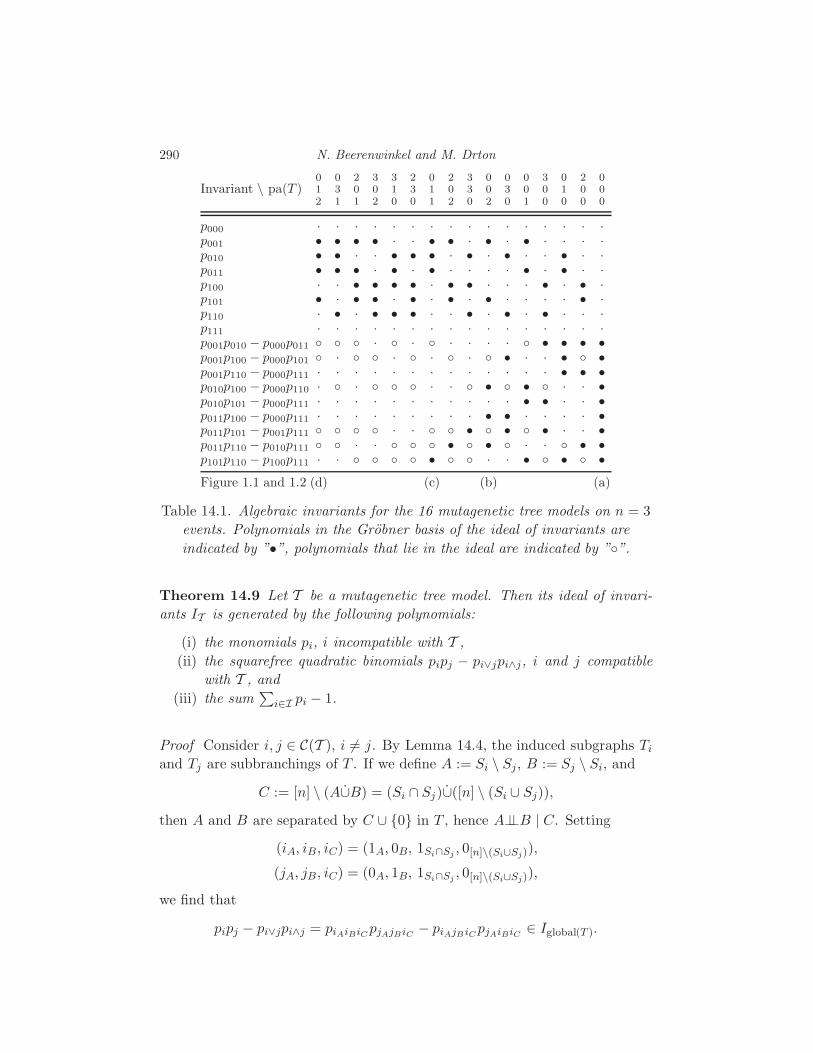
290 N. Beerenwinkel and M. Drton
Invariant \ pa(T )012
031
201
302
310
230
011
202
330
002
030
001
300
010
200
000
p000 · · · · · · · · · · · · · · · ·p001 • • • • · · • • · • · • · · · ·p010 • • · · • • • · • · • · · • · ·p011 • • • · • · • · · · · • · • · ·p100 · · • • • • · • • · · · • · • ·p101 • · • • · • · • · • · · · · • ·p110 · • · • • • · · • · • · • · · ·p111 · · · · · · · · · · · · · · · ·p001p010 − p000p011 · · · · · · • • • •p001p100 − p000p101 · · · · • · · • •p001p110 − p000p111 · · · · · · · · · · · · · • • •p010p100 − p000p110 · · · · • • · · •p010p101 − p000p111 · · · · · · · · · · · • • · · •p011p100 − p000p111 · · · · · · · · · • • · · · · •p011p101 − p001p111 · · • • • · · •p011p110 − p010p111 · · • • · · • •p101p110 − p100p111 · · • · · • • •Figure 1.1 and 1.2 (d) (c) (b) (a)
Table 14.1. Algebraic invariants for the 16 mutagenetic tree models on n = 3
events. Polynomials in the Grobner basis of the ideal of invariants are
indicated by ”•”, polynomials that lie in the ideal are indicated by ””.
Theorem 14.9 Let T be a mutagenetic tree model. Then its ideal of invari-
ants IT is generated by the following polynomials:
(i) the monomials pi, i incompatible with T ,
(ii) the squarefree quadratic binomials pipj − pi∨jpi∧j, i and j compatible
with T , and
(iii) the sum∑
i∈I pi − 1.
Proof Consider i, j ∈ C(T ), i 6= j. By Lemma 14.4, the induced subgraphs Ti
and Tj are subbranchings of T . If we define A := Si \ Sj, B := Sj \ Si, and
C := [n] \ (A∪B) = (Si ∩ Sj)∪([n] \ (Si ∪ Sj)),
then A and B are separated by C ∪ 0 in T , hence A⊥⊥B | C. Setting
(iA, iB, iC) = (1A, 0B, 1Si∩Sj , 0[n]\(Si∪Sj)),
(jA, jB, iC) = (0A, 1B, 1Si∩Sj , 0[n]\(Si∪Sj)),
we find that
pipj − pi∨jpi∧j = piAiBiCpjAjB iC − piAjB iCpjAiBiC ∈ Iglobal(T ).
Mutagenetic Tree Models 291
This establishes the inclusion 〈pipj − pi∨jpi∧j, i, j ∈ C(T )〉 ⊂ IT .
To prove that the stated list of polynomials generates IT , it suffices to con-
sider a saturated conditional independence statement A⊥⊥B | C, and to show
that
IA⊥⊥B|C ⊂⟨pipj − pi∨jpi∧j, i, j ∈ C(T )
⟩+⟨pi, i 6∈ C(T )
⟩.
So consider a generator g of IA⊥⊥B|C ,
g = piAiB iCpjAjBiC − piAjBiCpjAiBiC , (iA, iB, iC), (jA, jB, iC) ∈ I.
First, note that
piAiBiCpjAjBiC ∈ 〈pi | i 6∈ C(T )〉 ⇐⇒ piAjB iCpjAiBiC ∈ 〈pi | i 6∈ C(T )〉 .
Indeed, by Lemma 14.4, k 6∈ C(T ) if and only if there exists (u, v) ∈ E(T ) with
v ∈ V (Tk), but u 6∈ V (Tk). Since A and B are separated by C ∪ 0, such
an edge cannot connect A and B. Therefore, it can only appear in both sets
E(TiAiBiC ) ∪E(TjAjB iC) and E(TiAjB iC ) ∪E(TjAiBiC ).
Assume now that all four states defining g are compatible with T . Then
Lemma 14.7 implies that their joins and meets are also compatible. Moreover,
iAiBiC ∨ jAjBiC = iAjBiC ∨ jAiBiC =: i ∨ jiAiBiC ∧ jAjBiC = iAjBiC ∧ jAiBiC =: i ∧ j
and we can write
g = (piAiBiCpjAjB iC − pi∨jpi∧j) + (pi∨jpi∧j − piAjBiCpjAiB iC )
as an element of 〈pipj − pi∨jpi∧j, i, j ∈ C(T )〉.
Example 14.10 Let S be the mutagenetic tree model defined by the star
topology, i.e. the model of complete independence; cf. Figures 14.1(a). Then
S is the intersection of the probability simplex with the Segre variety
VSegre =
n⋂
k=1
V (pi1...inpj1...jn − pi1...ik−1jkik+1...inpj1...jk−1ikjk+1...jn , i, j ∈ I),
i.e. the image of the n-fold Segre embedding P1 × · · · × P1 → P2n−1. To see
this note that the minors defining the Segre variety lie in
〈pipj − pi∨jpi∧j, i, j ∈ I〉 ,
because both products of the binomials defining VSegre have the same join and
meet. Conversely, let i, j ∈ I, i 6= j. Then there is a sequence of pairs of states
(i, j) = (i(0), j(0)), . . . , (i(m+1), j(m+1)) = (i ∨ j, i ∧ j)

292 N. Beerenwinkel and M. Drton
such that for all l = 1, . . . , m, both i(l+1) and j(l+1) are obtained from i(l) and
j(l), respectively, by exchanging at most one index. Hence, the telescoping sum
pipj − pi∨jpi∧j =
m∑
l=0
(pi(l)pj(l) − pi(l+1)pj(l+1))
lies in ISegre.
Our goal is to find a subset of the generators in Theorem 14.9 that forms a
Grobner basis (compare Chapter 3). More precisely, we seek a Grobner basis
for the ideal
PT := 〈pipj − pi∧jpi∨j, i, j ∈ C(T )〉 + 〈pi | i 6∈ C(T )〉
generated by the homogeneous polynomials in IT . The lexicographic order of
binary vectors in the state space I induces the order
p0...0000 > p0...0001 > p0...0010 > p0...0011 > p0...0100 > · · · > p1...1111
among the pi, i ∈ I. With this order of the indeterminates we use a monomial
order in R[pi, i ∈ I] that selects the underlined terms in the set
GT = pipj − pi∨jpi∧j, i, j ∈ C(T ), (i ∧ j) < i < j < (i ∨ j) (14.5)
as the leading monomials, for example the reverse or the degree-reverse lexi-
cographic order. This monomial order is fixed for the rest of this chapter and
underlies all subsequent results. We first consider the case of the star S.
Lemma 14.11 The polynomials GS form a Grobner basis for PS .
Proof Let i, j, k, l ∈ C(S) = I such that i 6= j and k 6= l. Then (possibly
after relabeling the four states) there exists u ∈ Si \ Sj and v ∈ Sk \ Sl. Set
A := u, v and B := [n] \ A and consider the generic matrix(p(iA,iB)
)iA∈IA, iB∈IB
.
All 2×2 minors of this matrix are elements of GS , and they enjoy the Grobner
basis property. In particular, the S-polynomial
S(pipj − pi∨jpi∧j, pkpl − pk∨lpk∧l)
reduces to zero modulo GS . So, GS is a Grobner basis for PS by Buchberger’s
criterion (Theorem 3.10).
Lemma 14.12 The polynomials GT form a Grobner basis for 〈GT 〉 = 〈GS〉 ∩R[pi, i ∈ C(T )].
Mutagenetic Tree Models 293
Proof We first show the Grobner basis property
〈LT(GT )〉 = 〈LT(〈GS〉 ∩ R[pi, i ∈ C(T )])〉 .
Since GT ⊂ GS ∩ R[pi, i ∈ C(T )], one inclusion is obvious. For the other one,
let f ∈ 〈GS〉 ∩ R[pi, i ∈ C(T )]. By Lemma 14.11, LT(f) is divisible by LT(g)
for some
g = pipj − pi∧jpi∨j ∈ GS .
Since LT(f) ∈ R[pi, i ∈ C(T )], also LT(g) ∈ R[pi, i ∈ C(T )], i.e. i and j are
compatible with T . But then, by Lemma 14.7, i∧j and i∨j are also compatible
with T . Hence, g ∈ GS ∩ R[pi, i ∈ C(T )] = GT .
It remains to show that 〈GS〉 ∩ R[pi, i ∈ C(T )] = 〈GT 〉 but this follows from
the Grobner basis property of GT .
Theorem 14.13 For any mutagenetic tree T , the set GT ∪pi | i 6∈ C(T ) is a
reduced Grobner basis for the ideal PT generated by the homogeneous invariants
of T .
Proof By Buchberger’s criterion we need to show that all S-polynomials S(f, g)
of elements from GT ∪ pi | i 6∈ C(T ) reduce to zero. If both f and g are
elements of GT , this follows from Lemma 14.12. Otherwise, the leading terms
of f and g are relatively prime, and hence the S-polynomial reduces to zero.
The Grobner basis is reduced, because for any f ∈ GT ∪ pi | i 6∈ C(T ),no monomial of f lies in 〈LT((GT ∪ pi | i 6∈ C(T )) \ f)〉 by the definition
(14.5) of GT .
We note that these results can also be derived from work of [Hibi, 1987] on
algebras with straightening laws on distributive lattices. However, the self-
contained derivation given here emphasizes the unexpected relation to inde-
pendence statements and Bayesian networks.
Theorem 14.13 together with Algorithm 14.5 provides an efficient method for
computing a reduced Grobner basis for the ideal of invariants of a mutagenetic
tree model. This approach does not require implicitization (cf. Section 3.2)
and the computational complexity is linear in the size of the output, i.e. the
size of the Grobner basis.
Proposition 14.14 Let T be a mutagenetic tree on n events.
(i) The number of incompatible states is bounded from above by 2n −n−1.
This bound is attained if and only if T is a chain.
(ii) The cardinality of GT is bounded from above by(2n+1
2
)−3n. This bound
is attained if and only if T is the star S.

294 N. Beerenwinkel and M. Drton
Therefore, the cardinality of the Grobner basis in Theorem 14.13 is at most of
order O(4n).
Proof The number of compatible states is n + 1 for the chain model; cf.
Fig. 14.1(d). Any other tree topology has stricly more compatible states; cf.
Algorithm 14.5. This proves (i).
The polynomials in GS are indexed by the set of pairs (i, j) ∈ I2 with
(i ∧ j) < i < j < (i ∨ j). We write this index set as the difference
(i, j) ∈ I2 | i ≤ j \ (i, j) ∈ I2 | i ≤ j, Si ⊂ Sj. (14.6)
The cardinality of the first set is(2n+1
2
). For the second set, we group subsets
according to their cardinality. A subset of cardinality k has 2n−k supersets.
Hence, the second set has cardinality
n∑
k=0
(n
n− k
)2n−k =
n∑
k=0
(n
k
)2k1n−k = (1 + 2)n.
Since the second set in (14.6) is contained in the first one, the bound in (ii)
follows. For the tightness note that if (u, v), u 6= 0, is an edge of T , then the
polynomial indexed by (i, j) with Si = u and Sj = v is not in GT , because
j is not a compatible state.
14.3 Mixture Models
Let K ∈ N>0 and (T1, . . . , TK) be a family of K mutagenetic trees. Define the
map
f (T1,...,TK) : ∆K−1 × ΘK → ∆ = ∆2n−1
(λ, θ(1), . . . , θ(K)) 7→K∑
k=1
λk f (Tk)(θ(k)).(14.7)
Definition 14.15 The K-mutagenetic trees mixture model (T1, . . .TK) :=
f (T1,...,TK)(∆K−1 × ΘK) ⊂ ∆ is given by the map f (T1,...,TK). This algebraic
statistical model has parameter space ∆K−1 × ΘK and state space I.
A state i ∈ I is compatible with the K-mutagenetic trees mixture model
(T1, . . . , TK) if it is compatible with at least one of the mutagenetic tree models
Tk = f (Tk)(Θ), i.e. C(T1, . . . , TK) =⋃K
k=1 C(Tk).
Example 14.16 Consider the family (S, T ), where S is the star in Figure
14.1(a) and T the tree in Figure 14.1(b). All states i ∈ I are compatible

Mutagenetic Tree Models 295
with the resulting mixture model (S, T ). Two example coordinates of the map
f (S,T ) are
f101(λ, θ, θ) = λθ111(1− θ211)θ311,
f100(λ, θ, θ) = λθ111(1− θ211)(1− θ311) + (1− λ)θ111(1− θ211).
The coordinates of the map f (T1,...,TK) defining a mutagenetic trees mix-
ture model are multilinear (cf. Example 1.7). The EM algorithm described in
Chapter 1 permits to compute the maximum likelihood estimates for mixture
models of mutagenetic trees [Beerenwinkel et al., 2004].
Mutagenetic trees mixture models are, like mixture models in general, diffi-
cult to study algebraically. Let us consider an example.
Example 14.17 Let (T1, T2) be the family of mutagenetic trees defined by
the parent vectors pa(T1) = (2, 0, 0, 3) and pa(T2) = (0, 0, 2, 3). The resulting
mixture model (T1, T2) is of dimension 8. The reduced degree-reverse lexico-
graphic Grobner basis for the ideal of invariants contains the 6 polynomials pi,
i 6∈ C(T1, T2) = C(T1)∪C(T2), the sum∑
i∈I pi−1, and the degree-5 polynomial
p0011p0110p0111p1000p1110 − p0010p20111p1000p1110 − p2
0011p0110p1100p1110 + . . .
with 51 terms.
14.3.1 Secant Varieties
Consider the family (T, T ) of two mutagenetic trees, in which a single tree is
repeated. Then every distribution p ∈ (T , T ) is a convex combination of two
distributions pT , p′T ∈ T , i.e. p = λpT +(1−λ)p′T , λ ∈ [0, 1]. Therefore, (T , T )
is a subset of the intersection of the probability simplex ∆ with the first secant
variety of f (T )(CI), i.e. the Zariski closure of the set λpT + (1 − λ)p′T | λ ∈C, pT 6= p′T ∈ CI. This is the correspondence between mixture models and
secant varieties mentioned on page 1; see also Chapter 3.
If T is a chain, then every node in T has at most one child and |C(T )| =
n + 1. The chain model T is equal to the n-dimensional variety obtained by
intersecting the probability simplex ∆ with the 2n − n− 1 hyperplanes pi = 0,
i 6∈ C(T ). Since C(T , T ) = C(T ) and T ⊂ (T , T ) it follows that the chain
mixture model is trivial in the sense that (T , T ) = T .
If T = S is the star, then the mixture model (S, S) is also known as a
naive Bayes model (compare Proposition 14.19). In algebraic terms it is the
first secant variety of the Segre variety. It has been shown that dim(S, S) =
min(2n+ 1, 2n − 1) in this case [Catalisano et al., 2002, Garcia, 2004].
Let us consider an example of a tree that is neither a chain nor the star.
296 N. Beerenwinkel and M. Drton
Example 14.18 Let T be the tree over n = 4 events with vector of parents
pa(T ) = (2, 0, 0, 3). Then dim(T , T ) = 7, whereas dim(T ) = 4. The reduced
degree-reverse lexicographic Grobner basis for the ideal of invariants of Mcontains the 7 polynomials pi, i 6∈ C(T , T ) = C(T ), the sum
∑i∈I pi − 1, as
well as a polynomial of degree 3 with 22 terms.
The K-mutagenetic trees mixture models resulting from repeating a single
tree K times correspond algebraically to the K-th secant variety of the single
tree model. The following proposition and its proof are in analogy to Theorem
14.6.
Proposition 14.19 Let T be a mutagenetic tree and K ∈ N>0. Let M be
the directed acyclic graph obtained from T by adding the edges (0, v), v ∈ [n],
from the root 0 to every node v. Associating a hidden random variable X0 with
K levels with the root node 0 induces a directed graphical model M with one
hidden variable. Then a probability distribution p ∈ ∆ is in the K-mutagenetic
trees mixture model (T, . . . , T ) if and only if p ∈ M and pi = 0 for all i 6∈ C(T ).
14.3.2 The Uniform Star as an Error Model
If the observations contain a state that is incompatible with a tree model
T , then the likelihood function of T is constant and equal to zero. Thus,
in the presence of false positives and false negatives the maximum likelihood
tree will often be the star or have a star-like topology despite the fact that
other pathways may be significantly overrepresented in the data. One way to
account for such states is to mix a mutagenetic tree with a uniform star model;
see [Szabo and Boucher, 2002] for an alternative approach.
Definition 14.20 Let S be the star over n events. The 1-dimensional uni-
form star model Suni := f (Suni)([0, 1]) ⊂ ∆ is given by the specialization map
f (Suni)(θ11) = f (S)(θ11, . . . , θ11).
Note that in the uniform star model the n events occur independently with
the same probability. This is our error model.
Algebraically the uniform star model is the intersection of the probabil-
ity simplex with the rational normal curve of degree n, i.e. the image of the
Veronese map P1 → Pn. To see this note that the coordinates of f only de-
pend on the number k = |Si| of occurred events: fi(θ11) = θk11(1 − θ11)
n−k.
This means that we can identify the ideal ISuni with its image in the ring
R[pk, k = 0, . . . , n] under the ring homomorphism induced by i 7→ |Si|. In this

Mutagenetic Tree Models 297
ring, ISuni is generated by the quadrics (Theorem 14.9)
pk1i1pk2
i2− pl1
j1pl2
j2, k1i1 + k2i2 = l1j1 + l2j2,
0 ≤ k1, k2, l1, l2 ≤ 2, 0 ≤ i1, i2, j1, j2 ≤ n.
These terms are exactly the 2 × 2 minors of the 2 × n matrix(p0 p1 p2 . . . pn−1
p1 p2 p3 . . . pn
),
the defining polynomials of the rational normal curve of degree n.
Proposition 14.21 Let n ≥ 3. Then for any n-dimensional mutagenetic tree
model T the mixture model (Suni, T ) has dimension n+ 2.
Proof Clearly, dim(Suni, T ) ≤ n + 2 because dim(T ) = n and dim(Suni) = 1.
Thus, we have to show that the dimension may not drop below n+ 2.
Consider first a tree T 6= S. It is easy to see that |I \ C(T )| ≥ 2, because
n ≥ 3. Choosing two states j, j ′ 6∈ C(T ) such that pj = pj′ = 0 for all p ∈ T ,
we obtain that the Jacobian matrix J of the map f (Suni,T ) is upper triangular
J =
(λ× JT ∗
0 Jj,j′
), where JT =
(∂fi
∂θv11
)
i∈C(T )\j,j′, v∈[n]
.
The matrix JT depends only on (θ111, . . . , θn11) and up to deletion of two rows
of zeros it is the Jacobian matrix of the map f (T ) and, thus, of full rank in the
interior of the parameter space of (Suni, T ). The matrix
Jj,j′ =
∂fj
∂λ∂fj
∂θ11
∂fj′
∂λ
∂fj′
∂θ11
depends only on (λ, θ11) and its determinant equals 1 − λ times a univariate
polynomial g(θ11). Since g has only finitely many roots, it holds almost ev-
erywhere that the matrix Jj,j′ is of full rank 2 and the Jacobian J of full rank
n + 2. Therefore, dim(Suni, T ) = n + 2; compare [Geiger et al., 2001].
If T = S is the star, then we know that the mixture model (Suni, S) is
obtained by parameter specialization from (S, S). As mentioned in Section
14.3.1, dim(S, S) = 2n + 1 and thus the Jacobian of the map f (S,S) is of full
rank 2n+ 1 almost everywhere. Now it follows from the chain rule that
∂f(Suni,S)i
∂θ11=∑
v∈[n]
∂f(S,S)i
∂θv11
∣∣θv11=θ11
,
which implies that the Jacobian of the map f (Suni,S) is of full rank n+ 2.
15
Catalog of Small Trees
Marta Casanellas
Luis David Garcia
Seth Sullivant
This chapter is concerned with the description of the Small Trees website which
can be found at the following web address:
http://www.math.tamu.edu/∼lgp/small-trees/small-trees.htmlThe goal of the website is to make available in a unified format various alge-
braic features of different phylogenetic models. In the first section, we describe
a detailed set of notational conventions for describing the phylogenetic models
on trees which are listed on this website. This includes conventions for writ-
ing down the parameterizations given a tree as well as describing the Fourier
transform and writing down phylogenetic invariants in Fourier coordinates.
The second section gives a brief description of each of the types of algebraic
information which are associated to a model and a tree on the Small Trees
website. The third section contains an example of a page on the website. The
final section is concerned with simulation studies of using algebraic invariants
to recover phylogenies using the invariants for the Kimura 3–parameter model.
15.1 Notational Conventions
15.1.1 Labeling trees
We assume that each phylogenetic model is presented with a particular tree T
together with a figure representing that tree. The figures of trees with up to
five leaves will be the ones that can be found on the Small Trees website.
15.1.1.1 Rooted trees
If T is a rooted tree, there is a distinguished vertex of T called the root and
labeled by the letter r. The tree T should be drawn with the root r at the top
of the figure and the edges of the tree below the root. Each edge in the tree is
labeled with a lowercase letter a, b, c, . . .. The edges are labeled in alphabetical
order starting at the upper left hand corner, proceeding left to right and top
298

Catalog of Small Trees 299
to bottom. The leaves are labeled with the numbers 1, 2, 3, . . . starting with
the left–most leaf and proceeding left to right. Figure 15.1 shows the “giraffe”
tree with four leaves and its labeling.
1 2 3 4
a b c
d e
Fig. 15.1. The giraffe tree on four leaves
15.1.1.2 Unrooted trees
If T is an unrooted tree, it should be drawn with the leaves in a circle. The
edges of T are labeled with lower–case letters a, b, c, . . . in alphabetical order
starting at the upper left–hand corner of the figure and proceeding left to right
and top to bottom. The leaves are labeled with the numbers 1, 2, 3, . . . starting
at the first leaf “left of 12 o’clock” and proceeding counterclockwise around the
perimeter of the tree. Figure 15.2 illustrates this on the “quartet” tree.
1
2 3
4
a b
c
d e
Fig. 15.2. The quartet tree on four leaves
15.1.2 Parameterizations
Associated to each node in a model is a random variable with two or four states
depending on whether we are looking at binary data or DNA data. In the case
of binary data these states are 0, 1 and for DNA data they are A,C,G, Tin this order.
15.1.2.1 Root Distribution
The root distribution is a vector of length two or four depending on whether
the model is for binary or DNA sequences. The name of this vector is r. Its

300 M. Casanellas, L. D. Garcia, and S. Sullivant
entries are parameters r0, r1, r2, . . . and are filled in from left to right and are
recycled as the model requires.
Example 15.1 In the general strand symmetric model r always denotes the
vector
r = (r0, r1, r1, r0).
We tacitly assume that the entries in r sum to 1, though we do not eliminate
a parameter to take this into account. If the model assumes a uniform root
distribution, then r has the form r = (1/2, 1/2) or r = (1/4, 1/4, 1/4, 1/4)
according to whether the model is for binary or DNA data.
15.1.2.2 Transition Matrices
In each type of model, the letters a, b, c, . . . which label the edges are also
the transition matrices in the model. These are either 2×2 or 4×4 matrices
depending on whether the model is a model for binary data or DNA data.
In each case, the matrix is filled from left to right and top to bottom with
unknown parameters, recycling a parameter whenever the model requires it.
For the transition matrix of the edge labeled with x these entries are called
x0, x1, x2, . . ..
Example 15.2 For example, in the Kimura 3–parameter model the letter a
represents the matrix
a =
a0 a1 a2 a3
a1 a0 a3 a2
a2 a3 a0 a1
a3 a2 a1 a0
.
The Kimura 2–parameter and Jukes–Cantor models give rise to specializa-
tions of the parameters in the Kimura 3–parameter model, and hence the
letters denoting the parameters are recycled. For instance, the letter c in the
Jukes–Cantor DNA model and the letter d in the Kimura 2–parameter model
represent the following matrices
c =
c0 c1 c1 c1c1 c0 c1 c1c1 c1 c0 c1c1 c1 c1 c0
, d =
d0 d1 d2 d1
d1 d0 d1 d2
d2 d1 d0 d1
d1 d2 d1 d0
.
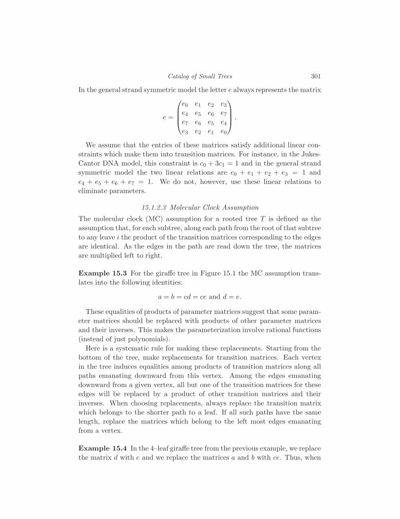
Catalog of Small Trees 301
In the general strand symmetric model the letter e always represents the matrix
e =
e0 e1 e2 e3e4 e5 e6 e7e7 e6 e5 e4e3 e2 e1 e0
.
We assume that the entries of these matrices satisfy additional linear con-
straints which make them into transition matrices. For instance, in the Jukes-
Cantor DNA model, this constraint is c0 + 3c1 = 1 and in the general strand
symmetric model the two linear relations are e0 + e1 + e2 + e3 = 1 and
e4 + e5 + e6 + e7 = 1. We do not, however, use these linear relations to
eliminate parameters.
15.1.2.3 Molecular Clock Assumption
The molecular clock (MC) assumption for a rooted tree T is defined as the
assumption that, for each subtree, along each path from the root of that subtree
to any leave i the product of the transition matrices corresponding to the edges
are identical. As the edges in the path are read down the tree, the matrices
are multiplied left to right.
Example 15.3 For the giraffe tree in Figure 15.1 the MC assumption trans-
lates into the following identities:
a = b = cd = ce and d = e.
These equalities of products of parameter matrices suggest that some param-
eter matrices should be replaced with products of other parameter matrices
and their inverses. This makes the parameterization involve rational functions
(instead of just polynomials).
Here is a systematic rule for making these replacements. Starting from the
bottom of the tree, make replacements for transition matrices. Each vertex
in the tree induces equalities among products of transition matrices along all
paths emanating downward from this vertex. Among the edges emanating
downward from a given vertex, all but one of the transition matrices for these
edges will be replaced by a product of other transition matrices and their
inverses. When choosing replacements, always replace the transition matrix
which belongs to the shorter path to a leaf. If all such paths have the same
length, replace the matrices which belong to the left most edges emanating
from a vertex.
Example 15.4 In the 4–leaf giraffe tree from the previous example, we replace
the matrix d with e and we replace the matrices a and b with ce. Thus, when

302 M. Casanellas, L. D. Garcia, and S. Sullivant
we write the parameterization in probability coordinates only the letters c and
e will appear in the parameterizing polynomials.
15.1.2.4 Specifying the Joint Distribution
The probabilities of the leaf colorations of a tree with n leaves are denoted
by pW where W is a word of length n in the alphabet 0, 1 or A,C,G, T.Every probability indeterminate pW is a polynomial in the parameters of the
model. Two of these probabilities pW and pU are equivalent if their defining
polynomials are identical. This divides the 2n or 4n probabilities into equiva-
lence classes. The elements of each class are ordered lexicographically, and the
classes are ordered lexicographically by their lexicographically first elements.
Example 15.5 For the Jukes–Cantor DNA model with uniform root distri-
bution on a three taxa claw tree there are five equivalence classes:
• Class 1: pAAA pCCC pGGG pTTT
• Class 2: pAAC pAAG pAAT pCCA pCCG pCCT pGGA pGGC pGGT pTTA pTTC
pTTG
• Class 3: pACA pAGA pATA pCAC pCGC pCTC pGAG pGCG pGTG pTAT pTCT
pTGT
• Class 4: pACC pAGG pATT pCAA pCGG pCTT pGAA pGCC pGTT pTAA pTCC
pTGG
• Class 5: pACG pACT pAGC pAGT pATC pATG pCAG pCAT pCGA pCGT pCTA
pCTG pGAC pGAT pGCA pGCT pGTA pGTC pTAC pTAG pTCA pTCG pTGA pTGC
For each class i there will be an indeterminate pi which denotes the sum of
the probabilities in the class i. For these N probabilities the expression for the
probability pi as a polynomial or rational function in the parameters appears
on the webpage (if these expressions are small enough) or in a separate linked
page for longer expressions.
Example 15.6 In the 3–taxa claw tree with Jukes–Cantor model and uniform
root distribution these indeterminates are:
p1 = a0b0c0 + 3a1b1c1p2 = 3a0b0c1 + 3a1b1c0 + 6a1b1c1p3 = 3a0b1c0 + 3a1b0c1 + 6a1b1c1p4 = 3a1b0c0 + 3a0b1c1 + 6a1b1c1p5 = 6a0b1c1 + 6a1b0c1 + 6a1b1c0 + 6a1b1c1
Note that p1+p2 +p3 +p4 +p5 = 1 after substituting a0 = 1−3a1, b0 = 1−3b1and c0 = 1− 3c1.
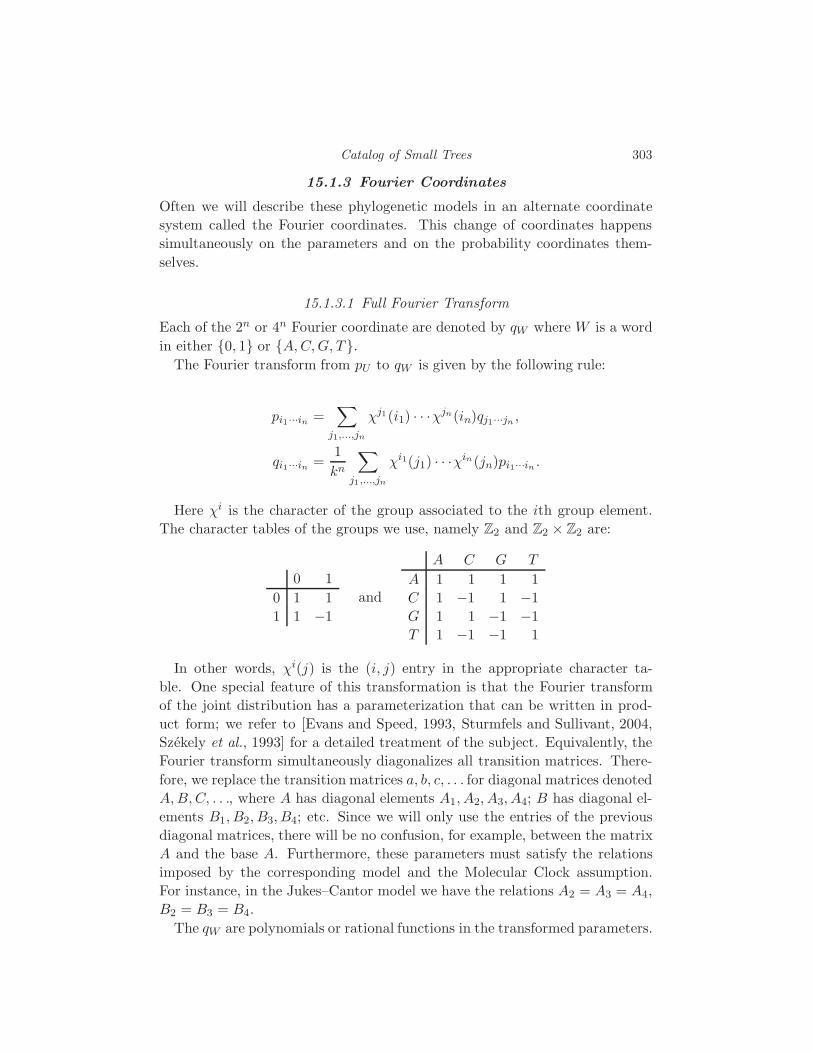
Catalog of Small Trees 303
15.1.3 Fourier Coordinates
Often we will describe these phylogenetic models in an alternate coordinate
system called the Fourier coordinates. This change of coordinates happens
simultaneously on the parameters and on the probability coordinates them-
selves.
15.1.3.1 Full Fourier Transform
Each of the 2n or 4n Fourier coordinate are denoted by qW where W is a word
in either 0, 1 or A,C,G, T.The Fourier transform from pU to qW is given by the following rule:
pi1···in =∑
j1,...,jn
χj1(i1) · · ·χjn(in)qj1···jn ,
qi1···in =1
kn
∑
j1,...,jn
χi1(j1) · · ·χin(jn)pi1···in .
Here χi is the character of the group associated to the ith group element.
The character tables of the groups we use, namely Z2 and Z2 × Z2 are:
0 1
0 1 1
1 1 −1
and
A C G T
A 1 1 1 1
C 1 −1 1 −1
G 1 1 −1 −1
T 1 −1 −1 1
In other words, χi(j) is the (i, j) entry in the appropriate character ta-
ble. One special feature of this transformation is that the Fourier transform
of the joint distribution has a parameterization that can be written in prod-
uct form; we refer to [Evans and Speed, 1993, Sturmfels and Sullivant, 2004,
Szekely et al., 1993] for a detailed treatment of the subject. Equivalently, the
Fourier transform simultaneously diagonalizes all transition matrices. There-
fore, we replace the transition matrices a, b, c, . . . for diagonal matrices denoted
A,B, C, . . ., where A has diagonal elements A1, A2, A3, A4; B has diagonal el-
ements B1, B2, B3, B4; etc. Since we will only use the entries of the previous
diagonal matrices, there will be no confusion, for example, between the matrix
A and the base A. Furthermore, these parameters must satisfy the relations
imposed by the corresponding model and the Molecular Clock assumption.
For instance, in the Jukes–Cantor model we have the relations A2 = A3 = A4,
B2 = B3 = B4.
The qW are polynomials or rational functions in the transformed parameters.
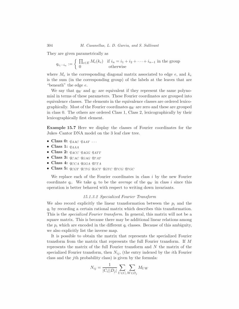
304 M. Casanellas, L. D. Garcia, and S. Sullivant
They are given parametrically as
qi1···in :=
∏e∈E Me(ke) if in = i1 + i2 + · · ·+ in−1 in the group
0 otherwise
where Me is the corresponding diagonal matrix associated to edge e, and ke
is the sum (in the corresponding group) of the labels at the leaves that are
“beneath” the edge e.
We say that qW and qU are equivalent if they represent the same polyno-
mial in terms of these parameters. These Fourier coordinates are grouped into
equivalence classes. The elements in the equivalence classes are ordered lexico-
graphically. Most of the Fourier coordinates qW are zero and these are grouped
in class 0. The others are ordered Class 1, Class 2, lexicographically by their
lexicographically first element.
Example 15.7 Here we display the classes of Fourier coordinates for the
Jukes–Cantor DNA model on the 3 leaf claw tree.
• Class 0: qAAC qAAT . . .
• Class 1: qAAA
• Class 2: qACC qAGG qATT
• Class 3: qCAC qGAG qTAT
• Class 4: qCCA qGGA qTTA
• Class 5: qCGT qCTG qGCT qGTC qTCG qTGC
We replace each of the Fourier coordinates in class i by the new Fourier
coordinate qi. We take qi to be the average of the qW in class i since this
operation is better behaved with respect to writing down invariants.
15.1.3.2 Specialized Fourier Transform
We also record explicitly the linear transformation between the pi and the
qi by recording a certain rational matrix which describes this transformation.
This is the specialized Fourier transform. In general, this matrix will not be a
square matrix. This is because there may be additional linear relations among
the pi which are encoded in the different qi classes. Because of this ambiguity,
we also explicitly list the inverse map.
It is possible to obtain the matrix that represents the specialized Fourier
transform from the matrix that represents the full Fourier transform. If M
represents the matrix of the full Fourier transform and N the matrix of the
specialized Fourier transform, then Nij, (the entry indexed by the ith Fourier
class and the jth probability class) is given by the formula:
Nij =1
|Ci||Dj|∑
U∈Ci
∑
W∈Dj
MUW

Catalog of Small Trees 305
where Ci is the ith equivalence class of Fourier coordinates and Dj is the
jth equivalence class of probability coordinates. We do not include the 0th
equivalence class of Fourier coordinates in the previous formula.
Example 15.8 In the Jukes–Cantor DNA model on the 3 leaf claw tree the
specialized Fourier transform matrix is
1 1 1 1 1
1 1 −13 −1
3 −13
1 −13 1 −1
3 −13
1 −13 −1
3 1 −13
1 −13 −1
3 −13
13
.
15.2 Description of website features
We give a brief description of the various items described on the website.
Dimension (D): The dimension of the model.
Degree (d): The degree of the model. Algebraically, this is defined as the
number of points in the intersection of the model and a generic (i.e. “random”)
subspace of dimension 4n minus the dimension of the model.
Maximum Likelihood Degree (mld): The maximum likelihood degree of
the model. See section 3.
Number of Probability Coordinates (np): Number of equivalences classes
of the probability coordinates. See the preceding section.
Number of Fourier Coordinates (nq): Number of equivalence classes of
Fourier coordinates without counting Class 0 (see the preceding section). This
is also the dimension of the smallest linear space that contains the model.
Specialized Fourier Transform: See the preceding section for a description.
Phylogenetic Invariants: A list of generators of the prime ideal of phyloge-
netic invariants. These are given in the Fourier coordinates.
Singularity Dimension (sD): The dimension of the set of singular points
on the model.
Singularity Degree (sd): The algebraic degree of the set of singular points
on the model.
15.3 Example
Here we describe the Jukes–Cantor model on the quartet tree (see Figure 15.2)
in more detail.
Dimension: D = 5 (note that there are only 5 independent parameters, one
for each transition matrix.)

306 M. Casanellas, L. D. Garcia, and S. Sullivant
Degree: d = 34.
Number of Probability Coordinates: np = 15 and the classes are repre-
sented by:
p1 = a0b0c0d0e0 + 3a1b0c1d1e0 + 3a0b1c1d0e1 + 3a1b1c0d1e1 + 6a1b1c1d1e1,
p2 = 3(a0b1c0d0e0 + 3a1b1c1d1e0 + a0b0c1d0e1 + 2a0b1c1d0e1
+ a1b0c0d1e1 + 2a1b1c0d1e1 + 2a1b0c1d1e1 + 4a1b1c1d1e1),
p3 = 3(a0b1c1d0e0 + a1b1c0d1e0 + 2a1b1c1d1e0 + a0b0c0d0e1
+ 2a0b1c1d0e1 + 2a1b1c0d1e1 + 3a1b0c1d1e1 + 4a1b1c1d1e1),
p4 = 3(a0b0c1d0e0 + a1b0c0d1e0 + 2a1b0c1d1e0 + a0b1c0d0e1
+ 2a0b1c1d0e1 + 2a1b1c0d1e1 + 7a1b1c1d1e1),
p5 = 6(a0b1c1d0e0 + a1b1c0d1e0 + 2a1b1c1d1e0 + a0b1c0d0e1 + a0b0c1d0e1
+ a0b1c1d0e1 + a1b0c0d1e1 + a1b1c0d1e1 + 2a1b0c1d1e1 + 5a1b1c1d1e1),
p6 = 3(a1b0c1d0e0 + a0b0c0d1e0 + 2a1b0c1d1e0 + a1b1c0d0e1
+ 2a1b1c1d0e1 + 2a1b1c0d1e1 + 3a0b1c1d1e1 + 4a1b1c1d1e1),
p7 = 3(a1b1c1d0e0 + a0b1c0d1e0 + 2a1b1c1d1e0 + a1b0c0d0e1 + 2a1b1c1d0e1
+ 2a1b1c0d1e1 + a0b0c1d1e1 + 2a1b0c1d1e1 + 2a0b1c1d1e1 + 2a1b1c1d1e1),
p8 = 6(a1b1c1d0e0 + a0b1c0d1e0 + 2a1b1c1d1e0 + a1b1c0d0e1
+ a1b0c1d0e1 + a1b1c1d0e1 + a1b0c0d1e1 + a1b1c0d1e1
+ a0b0c1d1e1 + a1b0c1d1e1 + 2a0b1c1d1e1 + 3a1b1c1d1e1),
p9 = 3(a1b1c0d0e0 + a0b1c1d1e0 + 2a1b1c1d1e0 + a1b0c1d0e1 + 2a1b1c1d0e1
+ a0b0c0d1e1 + 2a1b1c0d1e1 + 2a1b0c1d1e1 + 2a0b1c1d1e1 + 2a1b1c1d1e1),
p10 = 3(a1b0c0d0e0 + a0b0c1d1e0 + 2a1b0c1d1e0 + 3a1b1c1d0e1
+ a0b1c0d1e1 + 2a1b1c0d1e1 + 2a0b1c1d1e1 + 4a1b1c1d1e1),
p11 = 6(a1b1c0d0e0 + a0b1c1d1e0 + 2a1b1c1d1e0 + a1b0c1d0e1
+ 2a1b1c1d0e1 + a1b0c0d1e1 + a0b1c0d1e1 + a1b1c0d1e1
+ a0b0c1d1e1 + a1b0c1d1e1 + a0b1c1d1e1 + 3a1b1c1d1e1),
p12 = 6(a1b1c1d0e0 + a1b1c0d1e0 + a0b1c1d1e0 + a1b1c1d1e0
+ a1b1c0d0e1 + a1b0c1d0e1 + a1b1c1d0e1 + a0b0c0d1e1
+ a1b1c0d1e1 + 2a1b0c1d1e1 + 2a0b1c1d1e1 + 3a1b1c1d1e1),
p13 = 6(a1b1c1d0e0 + a1b1c0d1e0 + a0b1c1d1e0 + a1b1c1d1e0
+ a1b0c0d0e1 + 2a1b1c1d0e1 + a0b1c0d1e1 + a1b1c0d1e1
+ a0b0c1d1e1 + 2a1b0c1d1e1 + a0b1c1d1e1 + 3a1b1c1d1e1),

Catalog of Small Trees 307
p14 = 6(a1b0c1d0e0 + a1b0c0d1e0 + a0b0c1d1e0 + a1b0c1d1e0 + a1b1c0d0e1
+ 2a1b1c1d0e1 + a0b1c0d1e1 + a1b1c0d1e1 + 2a0b1c1d1e1 + 5a1b1c1d1e1),
p15 = 6(a1b1c1d0e0 + a1b1c0d1e0 + a0b1c1d1e0 + a1b1c1d1e0 + a1b1c0d0e1
+ a1b0c1d0e1 + a1b1c1d0e1 + a1b0c0d1e1 + a0b1c0d1e1 + a0b0c1d1e1
+ a1b0c1d1e1 + a0b1c1d1e1 + 4a1b1c1d1e1).
Number of Fourier Coordinates: nq = 13. The classes are:
q1 = qAAAA,
q2 = qAACC , qAAGG, qAATT ,
q3 = qACAC , qAGAG, qATAT ,
q4 = qACCA, qAGGA, qATTA,
q5 = qACGT , qACTG, qAGCT , qAGTC , qATCG, qATGC ,
q6 = qCAAC , qGAAG, qTAAT ,
q7 = qCACA, qGAGA, qTATA,
q8 = qCAGT , qCATG, qGACT , qGATC , qTACG, qTAGC ,
q9 = qCCAA, qGGAA, qTTAA,
q10 = qCCCC , qCCGG, qCCTT , qGGCC , qGGGG, qGGTT ,
qTTCC , qTTGG, qTTTT ,
q11 = qCGAT , qCTAG, qGCAT , qGTAC , qTCAG, qTGAC ,
q12 = qCGCG, qCGGC , qCTCT , qCTTC , qGCCG, qGCGC ,
qGTGT , qGTTG, qTCCT , qTCTC , qTGGT , qTGTG,
q13 = qCGTA, qCTGA, qGCTA, qGTCA, qTCGA, qTGCA.
Specialized Fourier Transform:
1 1 1 1 1 1 1 1 1 1 1 1 1 1 1
1 −13 −1
3 1 −13 1 −1
3 −13 −1
3 1 −13 −1
3 −13 1 −1
3
1 −13 1 −1
3 −13 −1
3 1 −13 −1
3 1 −13 −1
3 1 −13 −1
3
1 1 −13 −1
3 −13 −1
3 −13 −1
3 1 1 1 −13 −1
3 −13 −1
3
1 −13 −1
3 −13
13 −1
3 −13
13 −1
3 1 −13
13 −1
3 −13
13
1 −13 1 −1
3 −13 1 −1
3 −13 1 −1
3 −13 1 −1
3 −13 −1
3
1 1 −13 −1
3 −13 1 1 1 −1
3 −13 −1
3 −13 −1
3 −13 −1
3
1 −13 −1
3 −13
13 1 −1
3 −13 −1
3 −13
13 −1
313 −1
313
1 1 1 1 1 −13 −1
3 −13 −1
3 −13 −1
3 −13 −1
3 −13 −1
3
1 −13 −1
3 1 −13 −1
3 1 −13 1 −1
3 −13 −1
3 −13 −1
3 1
1 −13 1 −1
3 −13 −1
3 −13
13 −1
3 −13
13 −1
3 −13
13
13
1 −13 −1
3 −13
13 −1
3 1 −13 −1
3 −13
13
13 −1
313 −1
3
1 1 −13 −1
3 −13 −1
3 −13 −1
3 −13 −1
3 −13
13
13
13
13
308 M. Casanellas, L. D. Garcia, and S. Sullivant
Phylogenetic Invariants: We computed the phylogenetic invariants using
the results of [Sturmfels and Sullivant, 2004]. The invariants of degree 2 are:
q1q10 − q2q9, q3q7 − q4q6, q3q8 − q5q6,
q4q8 − q5q7, q3q13 − q4q11, q3q12 − q5q11,
q4q12 − q5q13, q6q13 − q7q11, q6q12 − q8q11,
q7q12 − q8q13.
The invariants of degree 3 associated to the left interior vertex are:
q1q11q11 − q3q6q9, q1q11q13 − q3q7q9, q1q11q12 − q3q8q9,
q1q13q11 − q4q6q9, q1q13q13 − q4q7q9, q1q13q12 − q4q8q9,
q1q12q11 − q5q6q9, q1q12q13 − q5q7q9, q1q12q12 − q5q8q9,
q2q11q11 − q3q6q10, q2q11q13 − q3q7q10, q2q11q12 − q3q8q10,
q2q13q11 − q4q6q10, q2q13q13 − q4q7q10, q2q13q12 − q4q8q10,
q2q12q11 − q5q6q10, q2q12q13 − q5q7q10, q2q12q12 − q5q8q10.
The invariants of degree 3 associated to the right interior vertex are:
q1q5q5 − q3q4q2, q1q5q8 − q3q7q2, q1q5q12 − q3q13q2,
q1q8q5 − q6q4q2, q1q8q8 − q6q7q2, q1q8q12 − q6q13q2,
q1q12q5 − q11q4q2, q1q12q8 − q11q7q2, q1q12q12 − q11q13q2,
q9q5q5 − q3q4q10, q9q5q8 − q3q7q10, q9q5q12 − q3q13q10,
q9q8q5 − q6q4q10, q9q8q8 − q6q7q10, q9q8q12 − q6q13q10,
q9q12q5 − q11q4q10, q9q12q8 − q11q7q10, q9q12q12 − q11q13q10.
The maximum likelihood degree, the singularity dimension and the singular-
ity degree are computationally difficult to achieve and we have not been able
to compute them using computer algebra programs.
15.4 Using the invariants
In this section we report some of the experiments we have made for inferring
small trees using phylogenetic invariants. These experiments were made using
the invariants for trees with 4 taxa on the Kimura 3–parameter model that can
be found in our website [Casanellas et al., 2004] which were computed using
the Sturmfels–Sullivant theorem [Sturmfels and Sullivant, 2004]. The results
obtained show that phylogenetic invariants are an efficient method for tree
reconstruction.

Catalog of Small Trees 309
We implemented an algorithm that performs the following tasks. Given 4
DNA sequences s1, s2, s3, s4, it first counts the number of occurrences of each
pattern for the topology ((s1, s2), s3, s4). Then it changes these absolute fre-
quencies to Fourier coordinates. From this, we have the Fourier transforms in
the other two possible topologies for trees with 4 species. We then evaluate all
the phylogenetic invariants for the Kimura 3–parameter model in the Fourier
coordinates of each tree topology. We call sTf the absolute value of this eval-
uation for the polynomial f and tree topology T . From these values sTf f ,
we produce a score for each tree topology T , namely s(T ) =∑
f |sTf |. The
algorithm then chooses the topology that has minimum score.
There was an attempt to define the score as the Euclidean norm of the
values sTf , but from our experiments, we deduced that the 1–norm chosen
above performs better.
We then tested this algorithm for different sets of sequences. We used the
program evolver from the package PAML [Yang, 1997] to generate sequences
according to the Kimura 2–parameter model with transition/transversion ratio
equal to 2 (typical value of mammalian DNA). In what follows we describe the
different tests we made and the results we obtained.
We generated 4–taxa trees with random branch lengths uniformly distributed
between 0 and 1. We performed 600 tests for sequences of lengths between
1000 and 10,000. The percentage of trees correctly reconstructed can be seen
in Figure 15.3.
We observed that our method fails to reconstruct the right tree mainly when
the length of the interior edge of the tree is small compared to the other branch
lengths. More precisely, in the trees that cannot be correctly inferred, the
length of the interior edge is about 10% the average length of the other edges.
Our method was also tested by letting the edge lengths be normally dis-
tributed with a given mean µ. We chose the values 0.25, 0.05, 0.005 for the
mean µ, following [John et al., 2003]. We also let the standard deviation be
0.1µ. In this case, we tested DNA sequences of lengths ranging from 50 to
10,000. Here, we only display the results for sequences of length up to 1000, be-
cause we checked that for larger sequences, we always infer the correct tree. For
each sequence length in 50, 100, 200, 300, 400, 500, 600, 700, 800, 900, 1000, we
generated edge lengths normally distributed with mean µ using the data analy-
sis program R [R Development Core Team, 2004]. Consequently, we generated
100 sequences for each mean and sequence length. The results are presented
in Figure 15.4.
From Figure 15.4, we see that for µ = 0.25 or µ = 0.05, it is enough to
consider sequences of length 200 to obtain a 100% efficiency. A much smaller
mean such as µ = 0.0005 was also tested. In this case, an efficiency over 90%
was only obtained for sequences of length ≥ 3000.

310 M. Casanellas, L. D. Garcia, and S. Sullivant
2000 4000 6000 8000 10000
5060
7080
9010
0
Uniformly distributed edge lengths in (0,1)
Sequence length
Per
cent
age
of tr
ees
infe
rred
cor
rect
ly
1000 3000 5000 7000 9000
5565
7585
95
Fig. 15.3. Percentage of trees correctly reconstructed with random branch lengthsuniformly distributed between 0 and 1.
200 400 600 800 1000
5060
7080
9010
0
Mean=0.25
Sequence length
Per
cent
age
of tr
ees
infe
rred
cor
rect
ly
50 200 400 600 800 1000 200 400 600 800 1000
5060
7080
9010
0
Mean=0.05
Sequence length
Per
cent
age
of tr
ees
infe
rred
cor
rect
ly
50 200 400 600 800 1000 200 400 600 800 1000
5060
7080
9010
0
Mean=0.005
Sequence length
Per
cent
age
of tr
ees
infe
rred
cor
rect
ly
50 200 400 600 800 1000
Fig. 15.4. Percentage of trees correctly reconstructed with edge lengths normally dis-tributed with mean equal to 0.25, 0.05, 0.005.
The method presented here is by no means the unique form of using these
invariants, so different ways of using them can even improve the tests.
Acknowledgments
Marta Casanellas was partially supported by RyC program of “Ministerio de
Ciencia y Tecnologia”, BFM2003-06001 and BIO2000-1352-C02-02 of “Plan

Catalog of Small Trees 311
Nacional I+D” of Spain. Luis David Garcia was a postdoctoral fellow at the
Mathematical Science Research Institute. Seth Sullivant was supported by
a NSF graduate research fellowship. Much of the research in this chapter
occurred during a visit to University of California, Berkeley, and we are grateful
for their hospitality. We like to thank Serkan Hosten for all his help and
guidance throughout this project.
16
The Strand Symmetric Model
Marta Casanellas
Seth Sullivant
16.1 Introduction
This chapter is devoted to the study of strand symmetric Markov models
on trees from the standpoint of algebraic statistics. By a strand symmetric
Markov model, we mean one whose mutation structure reflects the symmetry
induced by the double-stranded structure of DNA. In particular, a strand sym-
metric model for DNA must have the following equalities of probabilities in
the root distribution:
πA = πT and πC = πG
and the following equalities of probabilities in the transition matrices (θij)
θAA = θTT , θAC = θTG, θAG = θTC , θAT = θTA,
θCA = θGT , θCC = θGG, θCG = θGC , θCT = θGA.
Important special cases of strand symmetric Markov models are the group-
based phylogenetic models including the Jukes-Cantor model and the Kimura
2 and 3 parameter models. The general strand symmetric model or in this
chapter just the strand symmetric model (SSM) has only these eight equalities
of probabilities in the transition matrices and no further restriction on the
transition probabilities. Thus, for each edge in the corresponding phylogenetic
model, there are 6 free parameters.
For the standard group-based models (i.e. Jukes-Cantor and Kimura), the
transition matrices and the entire parametrization can be simultaneously diag-
onalized by means of the Fourier transform of the group Z2 × Z2
[Evans and Speed, 1993, Szekely et al., 1993]. Besides the practical uses of the
Fourier transform for group based models (see for example
[Semple and Steel, 2003]), this diagonalization of the group-based models
makes it possible to compute phylogenetic invariants for these models, by re-
ducing the problem to the claw tree K1,3 [Sturmfels and Yu, 2004]. Our goal
312
The Strand Symmetric Model 313
in this chapter is to extend the Fourier transform from group-based models to
the strand symmetric model. This is carried out in Section 16.2.
In Section 16.3 we focus in on the case of the three taxa tree. The com-
putation of phylogenetic invariants for the SSM in the Fourier coordinates is
still not complete, though we report on what is known about these invariants.
In particular, we describe all invariants of degree three and four. Section 16.5
is concerned with extending known invariants from the three taxa tree to an
arbitrary tree. In particular, we describe how to extend the given degree three
and four invariants from Section 16.3 to an arbitrary binary tree. To do this,
we introduce G-tensors and explore their properties in Section 16.4.
In Section 16.6, we take up the task of extending the “gluing” results for
phylogentic invariants which appear both in the work of Allman and Rhodes
[Allman and Rhodes, 2004a] and Sturmfels and Sullivant
[Sturmfels and Sullivant, 2004]. Our exposition and inspiration mainly comes
from the work of Allman and Rhodes and we deduce that the problem of
determining defining phylogenetic invariants for the strand symmetric model
reduces to finding phylogenetic invariants for the claw tree K1,3. Here defining
means a set of polynomials which generate the ideal of invariants up to rad-
ical; that is, defining invariants have the same zero set as the whole ideal of
invariants. This result is achieved by proving some “block diagonal” versions
of results which appear in the Allman and Rhodes paper. This line of attack
is the heart of Sections 16.4 and 16.6.
16.2 Matrix-Valued Fourier Transform
In this section we introduce the matrix-valued group-based models and show
that the strand symmetric model is a matrix-valued group-based model. Then
we describe the matrix-valued Fourier transform and the resulting simplifica-
tion in the parametrization of these models. We make special emphasis on the
strand symmetric model.
Let T be a rooted tree with n taxa. First, we wish to describe the random
variables associated to each vertex in the tree in the matrix-valued group-based
models. Each random variable Xv takes on kl states where k is the cardinality
of a finite abelian group G. The states of the random variable are 2-ples(ji
)
where j ∈ G and i ∈ 0, 1, . . . , l− 1.Associated to the root node R in the tree is the root distribution Rj1
i1. For
each edge E of T the double indexed set of parameters Ej1j2i1i2
is the transition
matrix associated to this edge. We use the convention that E is both the
edge and the transition matrix associated to that edge, to avoid the need
for introducing a third index on the matrices. Thus Ej1j2i1i2
is the conditional
314 M. Casanellas and S. Sullivant
probability of making a transition from state(j1i1
)to state
(j2i2
)along the edge
E.
Definition 16.1 A phylogenetic model is a matrix-valued group-based model
if for each edge, the matrix transition probabilities satisfy
Ej1j2i1i2
= Ej3j4i1i2
when j1 − j2 = j3 − j4 (where the difference is taken in G) and the root
distribution probabilities satisfy Rj1i = Rj2
i .
Example 16.2 Consider the strand symmetric model and make the identifi-
cation of the states A =(00
), G =
(01
), T =
(10
), and C =
(11
). One can check
directly from the definitions that the strand symmetric model is a matrix-
valued group-based model with l = 2 and G = Z2.
To avoid some even more cumbersome notation, we will restrict attention to
binary trees T and to the strand symmetric model for DNA. While the results
of Section 16.3 and 16.5 are exclusive to the case of the SSM, all our other
results can be easily extended to arbitrary matrix-valued group-based models
with the introduction of the more general Fourier transform, though we will
not explain these generalizations here.
We assume all edges of T are directed away from the root R. Given an edge
E of T let s(E) denote the initial vertex of E and t(E) the trailing vertex.
Then the parametrization of the phylogenetic model is given as follows. The
probability of observing states j1j2...jn
i1i2...inat the leaves is
pj1j2...jn
i1i2...in=
∑
((jviv))∈H
RjRiR
∏
E
Ejs(E)jt(E)
is(E)it(E)
where the product is taken over all edges E of T and the sum is taken over the
set
H = ((jviv
))v∈IntV (T )|jv, iv ∈ 0, 1.
Here IntV (T ) denotes the interior or nonleaf vertices of T .
Example 16.3 For the three leaf claw tree, the parametrization is given by
the expression:
plmnijk = R0
0A0l0iB
0m0j C
0n0k + R1
0A1l0iB
1m0j C
1n0k +R0
1A0l1iB
0m1j C
0n1k + R1
1A1l1iB
1m1j C
1n1k .
The study of this particular tree will occupy a large part of the paper.
The Strand Symmetric Model 315
Because of the role of the group in determining the symmetry in the parame-
trization, the Fourier transform can be applied to make the parametri-zation
simpler. We will not define the Fourier transform in general, only in the specific
case of the group Z2. The Fourier transform applies to all of the probability
coordinates, the transition matrices and the root distribution.
Definition 16.4 The Fourier transform of the probability coordinates is
qj1j2...jni1i2...in
=∑
k1,k2,...,kn∈0,1
(−1)k1j1+k2j2+···+knjnpk1k2...kni1i2...in
.
The Fourier transform of the transition matrix E is
ej1j2i1i2
=1
2
∑
k1,k2∈0,1
(−1)k1j1+k2j2Ek1k2i1i2
.
The Fourier transform of the root distribution is
rji =
∑
k∈0,1
(−1)kjRki .
It is easy to check that ej1j2i1i2
= 0 if j1 + j2 = 1 ∈ Z2 and similarly that rji = 0
if j = 1. In particular, writing e as a matrix, we see that the Fourier transform
replaces the matrix E with a matrix e that is block diagonal. Generally, when
working with our “hands on” the parameters (in particular in Section 16.3)
we will write the transition matrices with only one superscript: eji1i2and the
transformed root distribution ri with no superscript at all, though at other
times it will be more convenient to have the extra superscript around, in spite
of their redundancy.
Lemma 16.5 In the Fourier coordinates the parametrization is given by the
rule
qj1j2...jn
i1i2...in=
∑
(iv)∈H
rjr
ir
∏
e
ejs(e)
is(e)it(e)
where js(e) is the sum of jl such that l is a leaf below s(e) in the tree, jr =
j1 + · · ·+ jn and H denotes the set
H = (iv)v∈IntV (T ) and iv ∈ 0, 1.
Proof We can rewrite the parametrization in the probability coordinates as
pk1k2...kni1i2...in
=∑
(iv)∈H
∑
(kv)∈H ′
RkRiR
∏
E
Eks(E)kt(E)
is(E)it(E)
316 M. Casanellas and S. Sullivant
where H is the set defined in the lemma and
H ′ = (kv)v∈IntV (T ) and kv ∈ Z2.The crucial observation is that for any fixed values of i1, . . . , in and (iv) ∈ H ,
the expression inside the parentheses is a standard group-based model for Z2.
Applying the Fourier transform we have the following expression for qj1j2...jni1i2...in
:
∑
k1,k2,...,kn∈0,1
(−1)k1j1+k2j2+···+knjn∑
(iv)∈H
∑
(kv)∈H ′
RkRiR
∏
E
Eks(E)kt(E)
is(E)it(E)
and interchanging summations
∑
(iv)∈H
∑
k1,k2,...,kn∈0,1
(−1)k1j1+k2j2+···+knjn∑
(kv)∈H ′
RkRiR
∏
E
Eks(E)kt(E)
is(E)it(E)
.
By our crucial observation above, the expression inside the large parenthe-
ses is the Fourier transform of a group-based model and hence by results
in [Evans and Speed, 1993] and [Szekely et al., 1993] the expression inside the
parentheses factors in terms of the Fourier transforms of the transition matri-
ces and root distribution in precisely the way illustrated in the statement of
the lemma.
Definition 16.6 Given a tree T , the projective variety of the SSM given by
the tree T is denoted by V (T ). The notation CV (T ) denotes the affine cone
over V (T ).
Proposition 16.7 (Linear Invariants)
qj1j2...jni1i2...in
= 0
if j1 + j2 + · · ·+ jn = 1 ∈ Z2.
Proof The equation j1+j2 + · · ·+jn = 1 ∈ Z2 implies that in the parametriza-
tion every summand involves r1ir for some ir. However, all of these parameters
are zero.
The linear invariants in the previous lemma are equivalent to the fact that
pj1j2...jn
i1i2...in= pj1j2...jn
i1i2...in
where j = 1− j ∈ Z2.
Up until now, we have implicitly assumed that all the matrices E involved
were actually matrices of transition probabilities and that the root distribution
R was an honest probability distribution. If we drop these conditions and look
The Strand Symmetric Model 317
at the parametrization in the Fourier coordinates, we can, in fact, drop r from
this representation altogether. That is, the variety parametrized by dropping
the transformed root distribution r is the cone over the Zariski closure of the
probabilistic parametrization.
Lemma 16.8 In the Fourier coordinates there is an open subset of CV (T ),
the cone over the strand symmetric model, that can be parametrized as
qj1j2...jni1i2...in
=∑
(iv)∈H
∏
e
ejs(e)
is(e)it(e)
when j1 + · · ·+ jn = 0 ∈ Z2, where js(e) is the sum of jl such that l is a leaf
below s(e) in the tree and H denotes the set
H = (iv)v∈IntV (T ) and iv ∈ 0, 1.
Proof Due to the structure of the reparametrization of the SSM which we will
prove in Section 16.4, it suffices to prove the lemma when T is the 3-leaf claw
tree K1,3. In this case, we are comparing the parametrizations
φ : qmnoijk = r0a
m0ib
n0jc
o0k + r1a
m1ib
n1jc
o1k
and
ψ : qmnoijk = dm
0ien0jf
o0k + dm
1ien1jf
o1k.
In the second case, there are no conditions on the parameters. In the first para-
metrization, the stochastic assumption on the root distribution and transition
matrices translates into the following restrictions on the Fourier parameters
r0 = 1, a0l0 + a0
l1 = 1, b0l0 + b0l1 = 1, c0l0 + c0l1 = 1
for l = 0, 1. We must show that for d, e, f belonging to some open subset U
we can choose r, a, b, c with the prescribed restrictions which realize the same
Q tensor up to scaling. To do this, define
δl = d0l0 + d0
l1, γl = e0l0 + e0l1, λl = f0l0 + f0
l1
for l = 0, 1 and take U the subset where these numbers are all non-zero. Set
amli = δ−1
l dmli , b
nlj = γ−1
l enlj, colk = λ−1
l folk, r0 = 1, and r1 =
δ1γ1λ1
δ0γ0λ0.
Clearly, all the parameters r, a, b, c satisfy the desired prescription. Further-
more, the parameterization with this choice of r, a, b, c differs from the original
parametrization by a factor of (δ0γ0λ0)−1. This proves that ψ(U) ⊂ Im(ψ) ⊂
CV (T ).On the other hand we have that V (T ) ⊂ Im(ψ) because we can always
take dmli = rla
mli , enlj = bnlj, f
olk = colk. Moreover it is clear that Im(ψ) is a cone
318 M. Casanellas and S. Sullivant
and hence CV (T ) ⊂ Im(ψ). The proof of the lemma is completed by taking
the Zariski closure.
Example 16.9 In the particular instance of the three leaf claw tree the Fourier
parametrization of the model is given by the formula
qmnoijk = am
0ibn0jc
o0k + am
1ibn1jc
o1k.
16.3 Invariants for the 3 taxa tree
In this section, we will describe the degree 3 and degree 4 phylogenetic in-
variants for the claw tree K1,3 on the strand symmetric model. We originally
found these polynomial invariants using the computational algebra package
Macaulay2 [Grayson and Stillman, 2002] though we will give a combinatorial
description of these invariants and proofs that they do, in fact, vanish on the
strand symmetric model.
It is still an open problem to decide whether or not the 32 cubics and 18
quartics described here generate the ideal of invariants, or even describe the
SSM set theoretically. Computationally, we determined that they generate
the ideal up to degree 4. Furthermore, one can show that neither the degree
3 nor the degree 4 invariants alone are sufficient to describe the variety set
theoretically.
16.3.1 Degree 3 Invariants
Proposition 16.10 For each l = 1, 2, 3 let ml, nl, ol, il, jl, kl be indices in
0, 1 such that ml+nl +ol = 0, m1 = m2, m3 = 1−m1, n1 = n3, n2 = 1−n1,
o2 = o3, and o1 = 1− o2 in Z2. Let f(m•, n•, o•, i•, j•, k•) be the polynomial in
the Fourier coordinates described as∣∣∣∣∣∣∣
qm1n1o1i1j1k1
qm2n1o1i2j1k1
0
qm1n2o2i1j2k2
qm2n2o2i2j2k2
qm3n3o2i3j3k2
qm1n2o3i1j2k3
qm2n2o3i2j2k3
qm3n3o3i3j3k3
∣∣∣∣∣∣∣−
∣∣∣∣∣∣∣
qm1n3o1i1j3k1
qm2n3o1i2j3k1
0
qm1n2o2i1j2k2
qm2n2o2i2j2k2
qm3n1o2i3j1k2
qm1n2o3i1j2k3
qm2n2o3i2j2k3
qm3n1o3i3j1k3
∣∣∣∣∣∣∣.
Then f(m•, n•, o•, i•, j•, k•) is a phylogenetic invariant for K1,3 on the SSM.
Remark 16.11 The only nonzero cubics invariants forK1,3 arising from Propo-
sition 1 are those satisfying i2 = 1− i1, i3 = i2,j2 = j1, j3 = 1− j1, k2 = 1−k1
and k3 = k1. We maintain all the indices because they are necessary when we
extend invariants to larger trees in section 16.5. In total, we obtain 32 invari-
ants in this way and we verified in Macaulay2 [Grayson and Stillman, 2002]
that these 32 invariants generate the ideal in degree 3.

The Strand Symmetric Model 319
Proof In order to prove this result it is very useful to write the parametrization
in Fourier coordinates as:
qmnoijk =
∣∣∣∣am
0ibn0j −co1k
am1ib
n1j co0k
∣∣∣∣ .
In f(m•, n•, o•, i•, j•, k•) we substitute the Fourier coordinates by their pa-
rametrization and we call D1 the first determinant and D2 the second one so
that
D1 =
∣∣∣∣∣∣∣∣∣∣∣∣∣∣∣
∣∣∣∣∣am1
0i1bn10j1
−co11k1
am11i1bn11j1
co10k1
∣∣∣∣∣
∣∣∣∣∣am2
0i2bn10j1
−co11k1
am21i2bn11j1
co10k1
∣∣∣∣∣ 0∣∣∣∣∣am1
0i1bn20j2
−co21k2
am11i1bn21j2
co20k2
∣∣∣∣∣
∣∣∣∣∣am2
0i2bn20j2
−co21k2
am21i2bn21j2
co20k2
∣∣∣∣∣
∣∣∣∣∣am3
0i3bn30j3
−co21k2
am31i3bn31j3
co20k2
∣∣∣∣∣∣∣∣∣∣am1
0i1bn20j2
−co31k3
am11i1bn21j2
co30k3
∣∣∣∣∣
∣∣∣∣∣am2
0i2bn20j2
−co31k3
am21i2bn21j2
co30k3
∣∣∣∣∣
∣∣∣∣∣am3
0i3bn30j3
−co31k3
am31i3bn31j3
co30k3
∣∣∣∣∣
∣∣∣∣∣∣∣∣∣∣∣∣∣∣∣
.
Now we observe that the indices in the first position are the same for each
column in both determinants involved in f(m•, n•, o•, i•, j•, k•). Similarly, the
indices in the third position are the same for each row in both determinants.
Using recursively the formula
∣∣∣∣∣∣∣∣
∣∣∣∣x1,1 y
x2,1 z
∣∣∣∣∣∣∣∣x1,2 y
x2,2 x
∣∣∣∣∣∣∣∣x1,3 y
x2,3 z
∣∣∣∣x3,1 x3,2 x3,3
x4,1 x4,2 x4,3
∣∣∣∣∣∣∣∣=
∣∣∣∣∣∣∣∣
x1,1 x1,2 x1,3 y
x2,1 x2,2 x2,3 z
x3,1 x3,2 x3,3 0
x4,1 x4,2 x4,3 0
∣∣∣∣∣∣∣∣
it is easy to see that D1 can be written as the following 6 × 6 determinant:
D1 =
∣∣∣∣∣∣∣∣∣∣∣∣∣
am10i1bn10j1
am20i2bn10j1
0 −co11k1
0 0
am11i1bn11j1
am21i2bn11j1
0 co10k1
0 0
am10i1bn20j2
am20i2bn20j2
am30i3bn30j3
0 −co21k2
0
am11i1bn21j2
am21i2bn21j2
am31i3bn31j3
0 co20k2
0
am10i1bn20j2
am20i2bn20j2
am30i3bn30j3
0 0 −co31k3
am11i1bn21j2
am21i2bn21j2
am31i3bn31j3
0 0 co30k3
∣∣∣∣∣∣∣∣∣∣∣∣∣
.
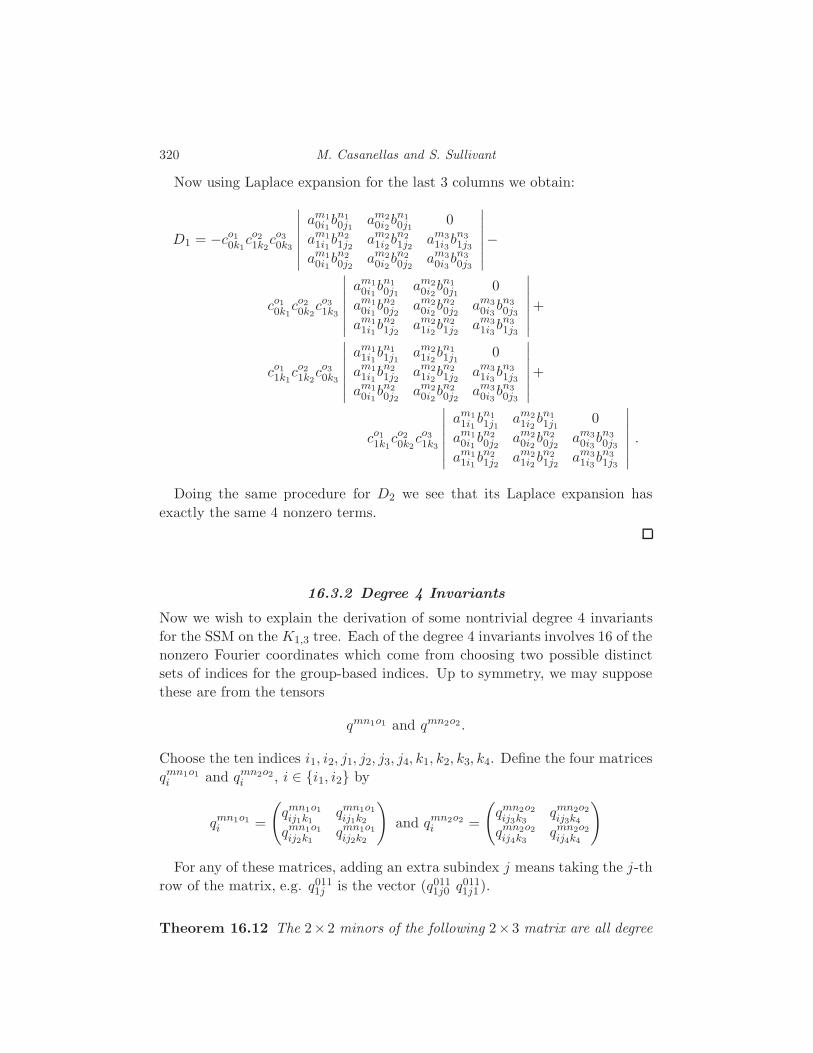
320 M. Casanellas and S. Sullivant
Now using Laplace expansion for the last 3 columns we obtain:
D1 = −co10k1co21k2co30k3
∣∣∣∣∣∣∣
am10i1bn10j1
am20i2bn10j1
0
am11i1bn21j2
am21i2bn21j2
am31i3bn31j3
am10i1bn20j2
am20i2bn20j2
am30i3bn30j3
∣∣∣∣∣∣∣−
co10k1co20k2co31k3
∣∣∣∣∣∣∣
am10i1bn10j1
am20i2bn10j1
0
am10i1bn20j2
am20i2bn20j2
am30i3bn30j3
am11i1bn21j2
am21i2bn21j2
am31i3bn31j3
∣∣∣∣∣∣∣+
co11k1co21k2co30k3
∣∣∣∣∣∣∣
am11i1bn11j1
am21i2bn11j1
0
am11i1bn21j2
am21i2bn21j2
am31i3bn31j3
am10i1bn20j2
am20i2bn20j2
am30i3bn30j3
∣∣∣∣∣∣∣+
co11k1co20k2co31k3
∣∣∣∣∣∣∣
am11i1bn11j1
am21i2bn11j1
0
am10i1bn20j2
am20i2bn20j2
am30i3bn30j3
am11i1bn21j2
am21i2bn21j2
am31i3bn31j3
∣∣∣∣∣∣∣.
Doing the same procedure for D2 we see that its Laplace expansion has
exactly the same 4 nonzero terms.
16.3.2 Degree 4 Invariants
Now we wish to explain the derivation of some nontrivial degree 4 invariants
for the SSM on the K1,3 tree. Each of the degree 4 invariants involves 16 of the
nonzero Fourier coordinates which come from choosing two possible distinct
sets of indices for the group-based indices. Up to symmetry, we may suppose
these are from the tensors
qmn1o1 and qmn2o2.
Choose the ten indices i1, i2, j1, j2, j3, j4, k1, k2, k3, k4. Define the four matrices
qmn1o1i and qmn2o2
i , i ∈ i1, i2 by
qmn1o1i =
(qmn1o1ij1k1
qmn1o1ij1k2
qmn1o1ij2k1
qmn1o1ij2k2
)and qmn2o2
i =
(qmn2o2ij3k3
qmn2o2ij3k4
qmn2o2ij4k3
qmn2o2ij4k4
)
For any of these matrices, adding an extra subindex j means taking the j-th
row of the matrix, e.g. q0111j is the vector (q011
1j0 q0111j1 ).
Theorem 16.12 The 2×2 minors of the following 2×3 matrix are all degree
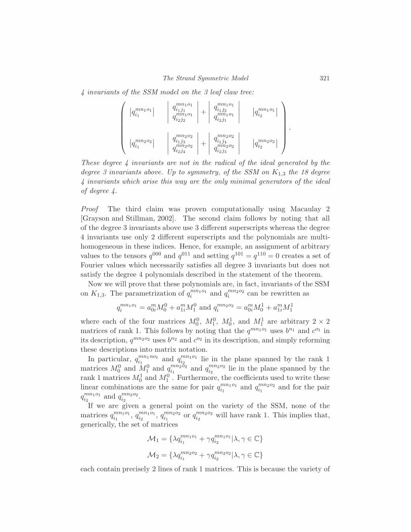
The Strand Symmetric Model 321
4 invariants of the SSM model on the 3 leaf claw tree:
∣∣qmn1o1i1
∣∣∣∣∣∣∣qmn1o1i1j1
qmn1o1i2j2
∣∣∣∣∣ +∣∣∣∣∣qmn1o1i1j2
qmn1o1i2j1
∣∣∣∣∣∣∣qmn1o1
i2
∣∣
∣∣qmn2o2i1
∣∣∣∣∣∣∣qmn2o2i1j3
qmn2o2i2j4
∣∣∣∣∣ +∣∣∣∣∣qmn2o2i1j4
qmn2o2i2j3
∣∣∣∣∣∣∣qmn2o2
i2
∣∣
.
These degree 4 invariants are not in the radical of the ideal generated by the
degree 3 invariants above. Up to symmetry, of the SSM on K1,3 the 18 degree
4 invariants which arise this way are the only minimal generators of the ideal
of degree 4.
Proof The third claim was proven computationally using Macaulay 2
[Grayson and Stillman, 2002]. The second claim follows by noting that all
of the degree 3 invariants above use 3 different superscripts whereas the degree
4 invariants use only 2 different superscripts and the polynomials are multi-
homogeneous in these indices. Hence, for example, an assignment of arbitrary
values to the tensors q000 and q011 and setting q101 = q110 = 0 creates a set of
Fourier values which necessarily satisfies all degree 3 invariants but does not
satisfy the degree 4 polynomials described in the statement of the theorem.
Now we will prove that these polynomials are, in fact, invariants of the SSM
on K1,3. The parametrization of qmn1o1i and qmn2o2
i can be rewritten as
qmn1o1i = am
0iM00 + am
1iM01 and qmn2o2
i = am0iM
10 + am
1iM11
where each of the four matrices M00 , M0
1 , M10 , and M1
1 are arbitrary 2 × 2
matrices of rank 1. This follows by noting that the qmn1o1 uses bn1 and co1 in
its description, qmn2o2 uses bn2 and co2 in its description, and simply reforming
these descriptions into matrix notation.
In particular, qmn1no1i1
and qmn1o1i2
lie in the plane spanned by the rank 1
matrices M00 and M0
1 and qmn2o2i1
and qmn2o2i2
lie in the plane spanned by the
rank 1 matrices M10 and M0
1 . Furthermore, the coefficients used to write these
linear combinations are the same for pair qmn1o1i1
and qmn2o2i1
and for the pair
qmn1o1i2
and qmn2o2i2
.
If we are given a general point on the variety of the SSM, none of the
matrices qmn1o1i1
, qmn1o1i2
, qmn2o2i1
or qmn2o2i2
will have rank 1. This implies that,
generically, the set of matrices
M1 = λqmn1o1i1
+ γqmn1o1i2
|λ, γ ∈ C
M2 = λqmn2o2i1
+ γqmn2o2i2
|λ, γ ∈ Ceach contain precisely 2 lines of rank 1 matrices. This is because the variety of

322 M. Casanellas and S. Sullivant
2×2 rank 1 matrices has degree 2. The set of values of λ and γ which produce
these lines of rank 1 matrices are the same because of the way that qmn1o1i1
,
qmn1o1i2
, qmn2o2i1
or qmn2o2i2
were written in terms of M00 , M0
1 , M10 and M1
1 . In
the first case, this set of λ and γ is the solution set of the quadratic equation∣∣λqmn1o1
i1+ γqmn1o1
i2
∣∣ = 0
and in the second case this set is the solution to the quadratic equation∣∣λqmn2o2
i1+ γqmn2o2
i2
∣∣ = 0.
To say that these two quadrics have the same zero set is equivalent to the
vanishing of the three 2 × 2 minors in the statement of the theorem. Since
the minors in the statement of the theorem vanish for a general point on the
parametrization they must vanish on the entire variety and hence are invariants
of the SSM.
16.4 G-tensors
In this section we introduce the notion of a G-tensor which should be regarded
as a multidimensional analog of a block diagonal matrix. We describe G-tensor
multiplication and a certain variety defined for G-tensors which will be useful
for extending invariants from the 3-leaf claw tree to arbitrary trees. This
variety GV (4r1, 4r2, 4r3) generalizes in a natural way the SSM on the claw tree
K1,3.
Notation. Let G be a group. For an n-tuple j = (j1, . . . , jn) ∈ Gn we denote
by σ(j) the sum j1 + · · ·+ jn ∈ G.
Definition 16.13 Let qj1···jni1···indefine a 4r1 ×· · ·×4rn tensor Q where the upper
indices are ri-tuples in the group G = Z2. We say that Q is G-tensor if
whenever σ(j1) + · · ·+ σ(jn) 6= 0 in G, qj1···jni1···in= 0. If n = 2 then Q is called a
G-matrix.
Lemma 16.14 If Q is a 4×· · ·×4 tensor arising from the SSM in the Fourier
coordinates, then Q is a G-tensor. All the Fourier parameter matrices ej1j2i1i2
are
G-matrices.
Proof This is immediate from Proposition 16.7 and the comments following
Definition 16.4.
Convention. Henceforth, we order any set of indices ( j1 · · · jti1 · · · it
)j1,...,jt,i1,...,it
so that we put first those indices whose upper sum σ(j) = j1 + · · ·+ jt is equal
to zero.
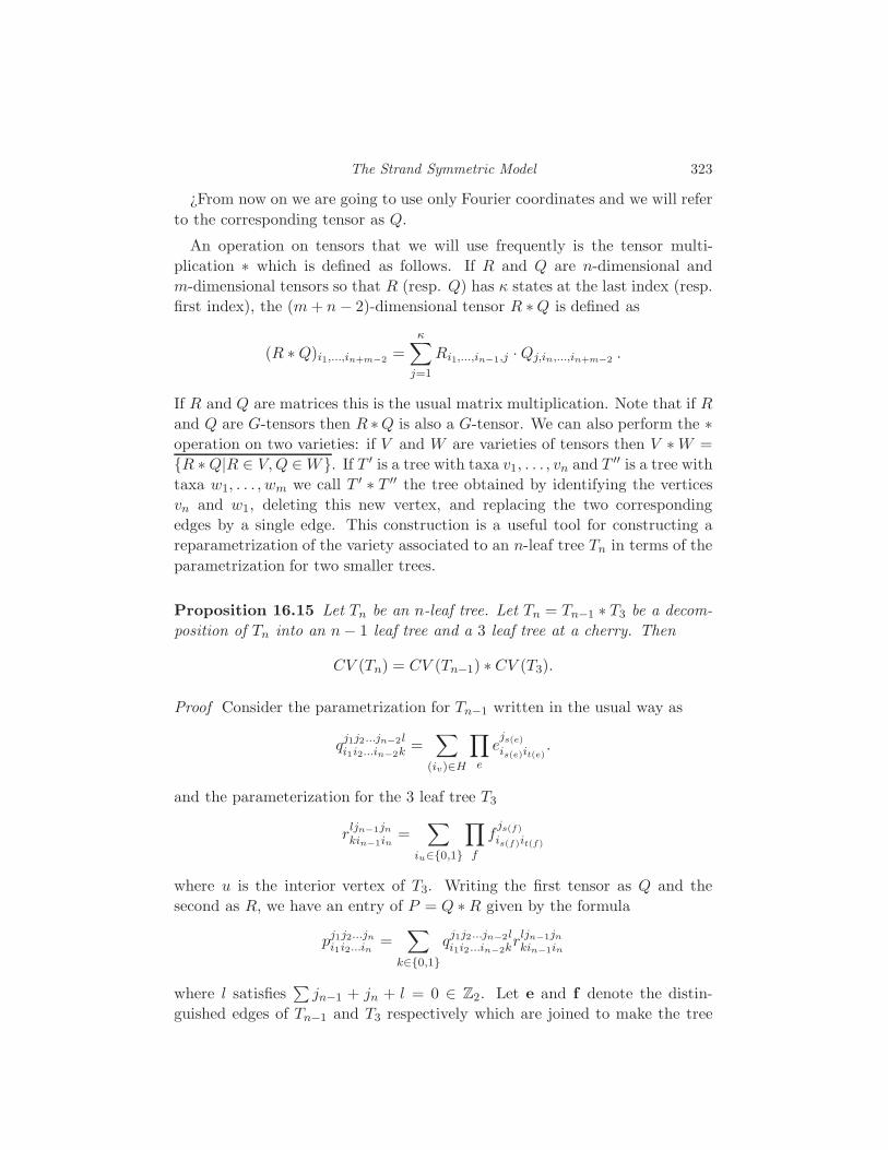
The Strand Symmetric Model 323
¿From now on we are going to use only Fourier coordinates and we will refer
to the corresponding tensor as Q.
An operation on tensors that we will use frequently is the tensor multi-
plication ∗ which is defined as follows. If R and Q are n-dimensional and
m-dimensional tensors so that R (resp. Q) has κ states at the last index (resp.
first index), the (m+ n − 2)-dimensional tensor R ∗Q is defined as
(R ∗Q)i1,...,in+m−2 =
κ∑
j=1
Ri1,...,in−1,j ·Qj,in,...,in+m−2 .
If R and Q are matrices this is the usual matrix multiplication. Note that if R
and Q are G-tensors then R ∗Q is also a G-tensor. We can also perform the ∗operation on two varieties: if V and W are varieties of tensors then V ∗W =
R ∗Q|R ∈ V, Q ∈W. If T ′ is a tree with taxa v1, . . . , vn and T ′′ is a tree with
taxa w1, . . . , wm we call T ′ ∗ T ′′ the tree obtained by identifying the vertices
vn and w1, deleting this new vertex, and replacing the two corresponding
edges by a single edge. This construction is a useful tool for constructing a
reparametrization of the variety associated to an n-leaf tree Tn in terms of the
parametrization for two smaller trees.
Proposition 16.15 Let Tn be an n-leaf tree. Let Tn = Tn−1 ∗ T3 be a decom-
position of Tn into an n− 1 leaf tree and a 3 leaf tree at a cherry. Then
CV (Tn) = CV (Tn−1) ∗ CV (T3).
Proof Consider the parametrization for Tn−1 written in the usual way as
qj1j2...jn−2li1i2...in−2k =
∑
(iv)∈H
∏
e
ejs(e)
is(e)it(e).
and the parameterization for the 3 leaf tree T3
rljn−1jn
kin−1in=
∑
iu∈0,1
∏
f
fjs(f)
is(f)it(f)
where u is the interior vertex of T3. Writing the first tensor as Q and the
second as R, we have an entry of P = Q ∗R given by the formula
pj1j2...jn
i1i2...in=
∑
k∈0,1
qj1j2...jn−2li1i2...in−2kr
ljn−1jn
kin−1in
where l satisfies∑jn−1 + jn + l = 0 ∈ Z2. Let e and f denote the distin-
guished edges of Tn−1 and T3 respectively which are joined to make the tree

324 M. Casanellas and S. Sullivant
Tn. Expanding the expression and regrouping yields
=∑
k∈0,1
∑
(iv)∈H
∏
e
ejs(e)
is(e)it(e)
∑
iv∈0,1
∏
f
fjs(f)
is(f)it(f)
=∑
(iv)∈H
∑
iu∈0,1
∑
k∈0,1
∏
e
ejs(e)
is(e)it(e)
∏
f
fjs(f)
is(f)it(f).
=∑
(iv)∈H
∑
iu∈0,1
∏
e6=e
ejs(e)
is(e)it(e)
∏
f 6=f
fjs(f)
is(f)it(f)
∑
k∈0,1
elis(e)ik
f likit(f)
.
The parenthesized expression is the product of the G-matrices e and f . Re-
placing this expression with a new single G-matrix of parameters along the
conjoined edge ef proves that CV (Tn−1) ∗CV (T3) ⊆ CV (Tn). Now expanding
the paramaterization given in Lemma 16.8 as a sum on the vertex u we obtain
the other inclusion.
Now we define a variety GV (4r1, 4r2, 4r3) which plays a large role when we
extend invariants.
Definition 16.16 For l = 1, 2, 3 let(jlil
)be a string of indices of length rl.
Let lM be an arbitrary G-matrix of size 4rl where the rows are indexed by
( 00 ) , ( 0
1 ) , ( 10 ) , ( 1
1 ) and the columns are indexed by the 4rl indices(jlil
).
Define the parametrization Q = ψr1,r2,r3(1M, 2M, 3M) by
Qj1j2j3i1i2i3
=∑
i∈0,1
1Mσ(j1)j1ii1 2M
σ(j2)j2ii2 3M
σ(j3)j3ii3
if σ(j1) + σ(j2) + σ(j3) = 0 and Qj1j2j3i1i2i3
= 0 if σ(j1) + σ(j2) + σ(j3) = 1. The
projective variety that is the Zariski closure of the image of ψr1,r2,r3 is denotedGV (4r1, 4r2, 4r3). The affine cone over this variety is CGV (4r1, 4r2, 4r3).
Remark 16.17 By the definition of GV (4r1, 4r2, 4r3) any Q ∈ GV (4r1, 4r2, 4r3)
is a G-tensor. Furthermore GV (4, 4, 4) is equal to the variety defined by the
SSM on the three leaf claw tree K1,3.
Besides the fact that GV (4r1, 4r2, 4r3) is equal to the SSM when r1 = r2 =
r3 = 1 the importance of this variety for the strand symmetric model comes
from the fact that GV (4r1, 4r2, 4r3) contains the SSM for any binary tree as
illustrated by the following proposition.

The Strand Symmetric Model 325
Proposition 16.18 Let T by a binary tree and v an interior vertex. Suppose
that removing v from T partitions the leaves of T into the three sets 1, . . . , r1,r1 + 1, · · · , r1 + r2, and r1 + r2 + 1 . . . , r1 + r2 + r3. Then the SSM on T
is a subvariety of GV (4r1, 4r2, 4r3).
In the proposition, the indices in the Fourier coordinates for the SSM are
grouped in the natural way according to the tripartition of the leaves.
Proof In the parametric representation
qj1j2...jn
i1i2...in=
∑
(iv)∈H
∏
e
ejs(e)
is(e)it(e)
perform the sum associated to the vertex v first. This realizes the G-tensor Q
as the sum over the product of entries of three G-tensors.
Our goal for the remainder of this section is to prove a result analogous
to Theorem 7 in Allman and Rhodes [Allman and Rhodes, 2004a]. This the-
orem will provide a method to explicitly determine the ideal of invariants
for GV (4r1, 4r2, 4r3) from the ideal of invariants for GV (4, 4, 4). Denote byGM(2l, 2m) the set of 2l× 2m G-matrices. A fundamental observation is that
if r3′ ≥ r3 then
CGV (4r1, 4r2, 4r′3) = CGV (4r1, 4r2, 4r3) ∗ GM(4r3, 4r′3).
Thus, we need to understand the ∗ operation when V and W are “well-
behaved” varieties.
Lemma 16.19 Let V ⊂ GM(2l, 4) be a variety and suppose that V ∗GM(4, 4) =
V . Let I be the vanishing ideal of V . Let K be the ideal of 3 × 3 G-minors
of the 2l × 2m G-matrix of indeterminates Q. Let Z be 2m × 4 G-matrix of
indeterminates and
L = 〈coeffZ(f(Q ∗ Z))|f ∈ gens(I)〉 .Then K + L is the vanishing ideal of W = V ∗ GM(4, 2m).
By a G-minor we mean a minor which involves only the nonzero entries in
the G-matrix Q.
Proof A useful fact is that
L =< f(Q ∗ A)|f ∈ I, A ∈ GM(2m, 4) > .
Let J be the vanishing ideal of W . By the definition of W , all the polynomials
in K must vanish on it. Moreover if f(Q ∗ A) is a polynomial in L, then it
vanishes at all the points of the form P ∗B, for any P ∈ V and B ∈ GM(4, 2m).
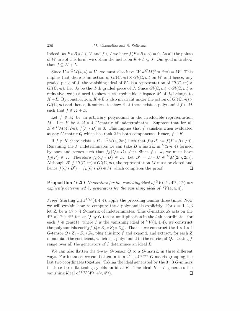
326 M. Casanellas and S. Sullivant
Indeed, as P ∗B ∗A ∈ V and f ∈ I we have f(P ∗B ∗A) = 0. As all the points
of W are of this form, we obtain the inclusion K+L ⊆ J. Our goal is to show
that J ⊆ K + L.
Since V ∗ GM(4, 4) = V , we must also have W ∗ GM(2m, 2m) = W . This
implies that there is an action of Gl(C, m)× Gl(C, m) on W and hence, any
graded piece of J, the vanishing ideal of W , is a representation of Gl(C, m)×Gl(C, m). Let Jd be the d-th graded piece of J. Since Gl(C, m)×Gl(C, m) is
reductive, we just need to show each irreducible subspace M of Jd belongs to
K+L. By construction, K+L is also invariant under the action of Gl(C, m)×Gl(C, m) and, hence, it suffices to show that there exists a polynomial f ∈M
such that f ∈ K + L.
Let f ∈ M be an arbitrary polynomial in the irreducible representation
M . Let P be a 2l × 4 G-matrix of indeterminates. Suppose that for all
B ∈ GM(4, 2m), f(P ∗ B) ≡ 0. This implies that f vanishes when evaluated
at any G-matrix Q which has rank 2 in both components. Hence, f ∈ K.
If f /∈ K there exists a B ∈ GM(4, 2m) such that fB(P ) := f(P ∗ B) 6 ≡0.
Renaming the P indeterminates we can take D a matrix in G(2m, 4) formed
by ones and zeroes such that fB(Q ∗ D) 6 ≡0. Since f ∈ J, we must have
fB(P ) ∈ I . Therefore fB(Q ∗ D) ∈ L. Let B′ = D ∗ B ∈ GM(2m, 2m).
Although B′ /∈ Gl(C, m)×Gl(C,m), the representation M must be closed and
hence f(Q ∗B′) = fB(Q ∗D) ∈M which completes the proof.
Proposition 16.20 Generators for the vanishing ideal of GV (4r1, 4r2, 4r3) are
explicitly determined by generators for the vanishing ideal of GV (4, 4, 4).
Proof Starting with GV (4, 4, 4), apply the preceding lemma three times. Now
we will explain how to compute these polynomials explicitly. For l = 1, 2, 3
let Zl be a 4rl × 4 G-matrix of indeterminates. This G-matrix Zl acts on the
4r1 × 4r2 × 4r3 tensor Q by G-tensor multiplication in the l-th coordinate. For
each f ∈ gens(I), where I is the vanishing ideal of GV (4, 4, 4), we construct
the polynomials coeffZf(Q ∗Z1 ∗Z2 ∗Z3). That is, we construct the 4× 4× 4
G-tensor Q ∗Z1 ∗Z2 ∗Z3, plug this into f and expand, and extract, for each Z
monomial, the coefficient, which is a polynomial in the entries of Q. Letting f
range over all the generators of I determines an ideal L.
We can also flatten the 3-way G-tensor Q to a G-matrix in three different
ways. For instance, we can flatten in to a 4r1 × 4r2+r3 G-matrix grouping the
last two coordinates together. Taking the ideal generated by the 3×3 G-minors
in these three flattenings yields an ideal K. The ideal K + L generates the
vanishing ideal of GV (4r1, 4r2, 4r3).

The Strand Symmetric Model 327
16.5 Extending invariants
In this section we will show how to derive invariants for arbitrary trees from
the invariants introduced in section 16.3. We also introduce the degree 3 de-
terminantal flattening invariants which arise from flatting the n-way G-tensor
associated to a tree T under the SSM along an edge of the tree. The idea
behind all of our results is to use the embedding of the SSM into the varietyGV (4r1, 4r2, 4r3).
Let T be a tree with n taxa on the SSM and let v be any interior vertex.
Removing v creates a tripartition of the leaves into three sets of cardinalities
r1, r2 and r3, which we may suppose, without loss of generality, are the sets
1, . . . , r1, r1 + 1, . . . , r1 + r2, and r1 + r2 + 1, . . . , r1 + r2 + r3.
Proposition 16.21 Let f(m•, n•, o•, i•, j•, k•) be one of the degree 3 invari-
ants for the 3 taxa treeK1,3 introduced in Proposition 16.10. For each l = 1, 2, 3
we choose sets of indices ml, il ∈ 0, 1r1, nl, jl ∈ 0, 1r2, and ol, kl ∈ 0, 1r3
such that σ(ml) = ml σ(nl) = nl and σ(ol) = ol. Then f(m•,n•, o•, i•, j•, k•)
=
∣∣∣∣∣∣∣
qm1n1o1
i1j1k1qm2n1o1
i2j1k10
qm1n2o2
i1j2k2qm2n2o2
i2j2k2qm3n3o2
i3j3k2
qm1n2o3
i1j2k3qm2n2o3
i2j2k3qm3n3o3
i3j3k3
∣∣∣∣∣∣∣−
∣∣∣∣∣∣∣
qm1n3o1
i1j3k1qm2n3o1
i2j3k10
qm1n2o2
i1j2k2qm2n2o2
i2j2k2qm3n1o2
i3j1k2
qm1n2o3
i1j2k3qm2n2o3
i2j2k3qm3n1o3
i3j1k3
∣∣∣∣∣∣∣
is a phylogenetic invariant for T.
Proof The polynomial f(m•,n•, o•, i•, j•, k•) must vanish on the varietyGV (4r1, 4r2, 4r3). This is because choosing m1, m2, . . . in the manner specified
corresponds to choosing a 3×3×3 subtensor of Q which belongs to a 4×4×4
G-subtensor ofQ (after flattening to a 3-way tensor). Since GV (4, 4, 4) arises as
a projection of GV (4r1, 4r2, 4r3) onto this G-subtensor, f(m•,n•, o•, i•, j•, k•)
belongs to the corresponding elimination ideal. Since the variety of the SSM
for T is contained in the variety GV (4r1, 4r2, 4r3), f(m•,n•, o•, i•, j•, k•) is an
invariant for the SSM on T .
Similarly, we can extend the construction of degree four invariants to arbi-
trary trees T by replacing the indices in their definition with vectors of indices.
We omit the proof which follows the same lines as the preceding proposition.
Proposition 16.22 Let m, il ∈ 0, 1r1, nl, jl ∈ 0, 1r2, and ol, kl ∈ 0, 1r3.
Then the three 2× 2 minors of the following matrix are all degree 4 invariants
328 M. Casanellas and S. Sullivant
of the SSM model on the tree T :
∣∣∣qmn1o1
i1
∣∣∣∣∣∣∣∣qmn1o1
i1j1
qmn1o1
i2j2
∣∣∣∣∣ +∣∣∣∣∣qmn1o1
i1j2
qmn1o1
i2j1
∣∣∣∣∣∣∣∣qmn1o1
i2
∣∣∣
∣∣∣qmn2o2
i1
∣∣∣∣∣∣∣∣qmn2o2
i1j3
qmn2o2
i2j4
∣∣∣∣∣ +∣∣∣∣∣qmn2o2
i1j4
qmn2o2
i2j3
∣∣∣∣∣∣∣∣qmn2o2
i2
∣∣∣
.
Now we wish to describe the determinantal edge invariants which arise by
flattening the G-tensor Q to a matrix along each edge of the tree. As we
shall see, there existence is already implied by our previous results, namely
Proposition 16.20. We make the special point of describing them here because
they will be useful in the next section.
Let e be an edge in the tree T . Removing this edge partitions the leaves
of T into two sets of size r1 and r2. The G-tensor Q flattens to a 4r1 × 4r2
G-matrix R. Denote by Fe the set of 3 × 3 G-minors of R.
Proposition 16.23 The 3× 3 G-minors Fe are invariants of the SSM on T .
Proof The edge e is incident to some interval vertex v of T . These 3 × 3
G-minors are in the ideal of say GV (4r1, 4r′2, 4r′3) associated to flattening the
tensor Q to a 3-way G tensor at this vertex. Then by Proposition 16.18 Fe are
invariants of the SSM on T .
16.6 Reduction to K1,3
In this section, we explain how the problem of computing defining invariants for
the SSM on a tree T reduces to the problem of computing defining invariants
on the claw tree K1,3. Our statements and proof are intimately related to the
results of Allman and Rhodes [Allman and Rhodes, 2004a] and we draw much
inspiration from their work.
Given an internal vertex v of T , denote by GVv the variety GV (4r1, 4r2, 4r3)
associated to flattening the G-tensor Q to a 3-way tensor according to the
tripartiiton induced by v.
Theorem 16.24 Let T be a binary tree. For each v ∈ IntV (T ) let Fv be a
set of invariants which define the variety GVv set theoretically. Then
CV (T ) = ∩v∈IntV (T )GVv
and hence
Fflat(T ) = ∪v∈IntV (T )Fv
are a defining set of invariants for the SSM on T .

The Strand Symmetric Model 329
The theorem reduces the computation of defining invariants to K1,3 since
a defining set of invariants for GV (4r1, 4r2, 4r3) can be determined from a set
of defining invariants for GV (4, 4, 4) = V (K1,3). Given the reparametrization
result of Section 16.4, it will suffice to show the following lemma, about the ∗operation on G-matrix varieties.
Lemma 16.25 Let V ⊆ GM(2l, 4) and W ⊆ GM(4, 2m) be two varieties such
that V = V ∗ GM(4, 4) and W = GM(4, 4) ∗W . Then
V ∗W =(V ∗ GM(4, 2m)
)∩(GM(2l, 4) ∗W
).
Proof Call the variety on the right hand side of the equality U . Since both of
the component varieties of U contain V ∗W , we must have V ∗W ⊆ U . Our
goal is to show the reverse inclusion. Let Q ∈ U . This matrix can be visualized
as a block diagonal matrix:
Q =
(Q0 0
0 Q1
).
Since Q ∈ U it must be the case that the rank of Q0 and Q1 are both less than
or equal to 2. Thus we can factorize Q as Q = R ∗ S where R ∈ GM(2l, 4)
and S ∈ GM(4, 2m). Without loss of generality, we may suppose that the
factorization Q = R ∗ S is nondegenerate in the sense that the rank of each
of the matrices R and S has only rank(Q) nonzero rows. Our goal is to show
that R ∈ V and S ∈W as this will imply the theorem.
By our assumption that the factorization Q = R ∗S is nondegenerate, there
exists a G-matrix A ∈ GM(2m, 4) such that Q∗A = R ∗S ∗A = R (A is called
the pseudo-inverse of S). Augmenting the matrix A with extra 0-columns, we
get a G-matrix A′ ∈ GM(2m, 2m). Then Q ∗ A′ ∈ V ∗ GM(4, 2m) since Q is
and V ∗ GM(4, 2m) is closed under multiplication by G-matrices on the right.
On the other hand, the natural projection of Q ∗A′ to GM(2l, 4) is Q ∗A = R.
Since the projection V ∗ GM(4, 2m) → GM(2l, 4) is the variety V because
V = V ∗ GM(4, 4), we have R ∈ V . A similar argument yields S ∈ W and
completes the proof.
Now we are in a position to give the proof the Theorem 16.24.
Proof We proceed by induction on n the number of leaves of T . If n = 3
there is nothing to show since this is the three leaf claw tree K1,3. Let T by
a binary n taxa tree. The tree T has a cherry T3, and thus we can represent
the tree T = Tn−1 ∗ T3 and the resulting variety as V (T ) = V (Tn−1) ∗ V (T3)
by the reparametrization. Now we apply the induction hypothesis to Tn−1
and T3. The varieties V (Tn−1) and V (T3) have the desired representation as

330 M. Casanellas and S. Sullivant
intersections of GVv. By the preceding Lemma, it suffices to show that this
representation extends to the variety V (Tn−1) ∗ GM(4, 16) and GM(4n−1, 4) ∗V (T3). This is almost immediate, since
GV (4r1, 4r2, 4r3) ∗ GM(4, 4s) = GV (4r1, 4r2, 4r3+s−1)
where GM(4, 4s) acts on a single index of GV (4r1, 4r2, 4r3) (recall thatGV (4r1, 4r2, 4r3) can be considered as either a 3-way tensor or an n-way 4 ×· · ·×4 tensor). This equation of varieties applies to each of the component va-
rieties in the intersection representation of V (Tn−1) and V (T3) and completes
the proof.
Acknowledgments
We would like to thank Bernd Sturmfels for some useful conversations about
this problem. Marta Casanellas was partially supported by RyC program of
“Ministerio de Ciencia y Tecnologia”, BFM2003-06001 and BIO2000-1352-C02-
02 of “Plan Nacional I+D” of Spain. Seth Sullivant was supported by a NSF
graduate research fellowship. Much of the research in this chapter occurred
during visits to University of California, Berkeley, and to the Universitat de
Barcelona (2001SGR-00071), and we are grateful for their hospitality.
17
Extending Tree Models to Split Networks
David Bryant
17.1 Introduction
In this chapter take statistical models designed for trees and generalize them to
more general constructions. In Chapter 2 we saw that phylogenetic trees can
be viewed as collections of pair-wise compatible splits (Theorem 2.34), where
each split corresponds to an edge in the tree. Thus a statistical model on a
tree is a statistical model on a collection of pair-wise compatible splits with
weights (or lengths). Our approach here is to drop the condition of pair-wise
compatibility and consider statistical models based on general collections of
splits and the split networks that represent them (Section 17.2).
Geometrically, the models we propose fill in the gaps between statistical
models for different trees. We show how we can relax the constraint that
limits analyses to tree-space. A relaxation of tree models can be used to test
statistically whether or not the data actually supports a tree. Split networks
provide natural swing-bridges between trees which could be used to compare
likelihood ratios or, in a Bayesian setting, used to estimate the ratio of Bayes
factors for two trees. The potential to relax the tree constraint also opens up
a huge range of new search techniques.
One of the more appealing applications of models based on split networks
is the representation of phylogenetic uncertainty. At present, the only widely
used way to represent uncertainty in an estimated phylogeny is to place con-
fidence values (such as posterior probabilities or bootstrap P -values) on the
branches of the phylogeny. A tree with confidence measures shows which part
of the phylogeny is less certain, but gives no indication of the nature of the
conflicting signal. Split networks, on the other hand, provide a means to repre-
sent confidence sets of trees in a single diagram, indicating both the uncertain
parts of the tree and any conflicting secondary signal.
A confusing aspect of split network models is that they are not explicit repre-
sentations of evolutionary history. Rather, they represent summary statistics,
statistics that are more informative than trees contain only a subset of the infor-
331

332 D. Bryant
mation present in a complete recombination history [Griffiths and Marjoram, 1996].
They are can therefore be more reliably estimated than complete reticulation
histories, and perhaps provide a stepping stone in the analysis. On the whole,
population geneticists don’t even dream to think that explicit recombination
histories can be reconstructed exactly. Instead they integrate out over differ-
ent histories and take summary statistics. Split networks are a particularly
informative and graphically appealing set of summary statistics to infer.
The outline of this chapter is:
• In section 17.2 we review the definitions of splits and split networks.
• In section 17.3 we discuss statistical models for split networks based on
distance data.
• In section 17.4 we briefly discuss, and critique, the application of graphical
models to split networks.
• In sections 17.5 to 17.7 we develop a character based model for splits net-
works based on the Fourier calculus for evolutionary trees studied by [Szekely et al., 1993].
• We conclude with open problems and some baseless speculation.
17.2 Trees, splits and split networks
Splits are the foundation of phylogenetic combinatorics, and they will be the
building blocks of our general statistical model. Recall (from Chapter 2) that
a split S = A,B of a finite set X is an unordered partition of X into two
non-empty blocks. An X-tree is a pair T = (T, φ) such that T is a tree and
φ : X → V (T ) is a map for which φ−1(v) is empty whenever v has degree less
than three. We say that T is a phylogenetic tree if T has no vertices of degree
two and φ is a bijection from X to the leaves of T .
Removing an edge e from an X-tree divides the tree into two connected
component, thereby inducing a split of X that we say is the split associated to
e. We use splits(T ) to denote the sets associated to edges of T . The X-tree
T can be reconstructed from the collection splits(T ). The Splits Equivalence
Theorem (Theorem 2.34) tells us that a collection S of splits equals splits(T )
for some X-tree T if and only if the collection is pairwise compatible, that is,
for all pairs of splits A,B, A′, B′ at least one of the intersections
A ∩A′, A ∩B′, B ∩ A′, B ∩ B′
is empty.
If we think ofX-trees as collections of compatible splits then it becomes easy
to generalize trees: we simply consider collections of splits that are not nec-
essarily pairwise compatible. This is the approach taken by Split Decomposi-
tion [Bandelt and Dress, 1992], Median Networks [Bandelt et al., 1995], Spec-
troNet [Huber et al., 2002], Neighbor-Net [Bryant and Moulton, 2004], Con-
Extending Tree Models to Split Networks 333
sensus Networks [Holland et al., 2004] and Z-networks [Huson et al., 2004], many
of which are implemented in the SplitsTree package[Huson, 1998, Huson and Bryant, 2005].
The usefulness of these methods is due to a particularly elegant graphical rep-
resentation for general collections of splits: the splits network.
To define splits networks, we first need to discuss splits graphs. These graphs
have multiple characterizations. We will work with three of these here.
In a graph G let dG denote the (unweighted) shortest path metric. A map
ψ from a graph H to a graph G is an isometric embedding if dH(u, v) =
dG(ψ(u), ψ(v)) for all u, v ∈ V (H). A graphG is a partial cube if there exists an
isometric embedding fromG to a hypercube. Wetzel [Wetzel, 1995] called these
graphs splits graphs. This terminology has persisted in the phylogenetics com-
munity, despite the potential for confusion with the graph-theoretic term ‘split
graph’ (a special class of perfect graphs). Refer to [Imrich and Klavzar, 2000]
for a long list of characterizations for partial cubes.
Wetzel [Wetzel, 1995] (see also Dress and Huson [Dress and Huson, 2004])
characterized splits graphs in terms of isometric colorings. Let σ be an edge
coloring of the graph. For each pair u, v ∈ V (G) let Cσ(u, v) denote the set of
colors appearing on all shortest paths between u and v. We say that σ is an
isometric coloring if dG(u, v) = |Cσ(u, v)| for all pairs u, v ∈ V (G). In other
words, σ is isometric if the edges along any shortest path all have different
colors, while any two shortest paths between the same pair of vertices have the
same set of edge colors. A connected graph is a splits graph if and only if it
has an isometric coloring [Wetzel, 1995].
A third characterization of splits graphs is due to [Winkler, 1984]. We define
a relation Θ on pairs off edges e1 = u1, v1 and e2 = u2, v2 in a graph G by
e1Θe2 ⇔ dG(u1, u2) + dG(v1, v2) 6= dG(u1, v2) + dG(v1, u2). (17.1)
This relation is an equivalence relation if and only if G is a splits graph.
Two edges e1 and e2 in a splits graph have the same color an isometric
coloring if and only if the isometric embedding of the splits graph maps e1 and
e2 to edges in the same dimension, if and only if e1Θe2. Thus, a splits graph
has, essentially, a unique isometric coloring and a unique isometric embedding
into the hypercube. The partition of edges into color classes is completely
determined by the graph.
Suppose now that we have a splits graph G and a map φ : X → V (G).
Using the isometric embedding, one can quickly prove that removing all edges
in a particular color class partitions the graph into exactly two connected (and
convex) components. This in turn induces a split of X , via the map φ. A splits
network is a pair N = (G, φ) such that
(i) G is a splits graph.
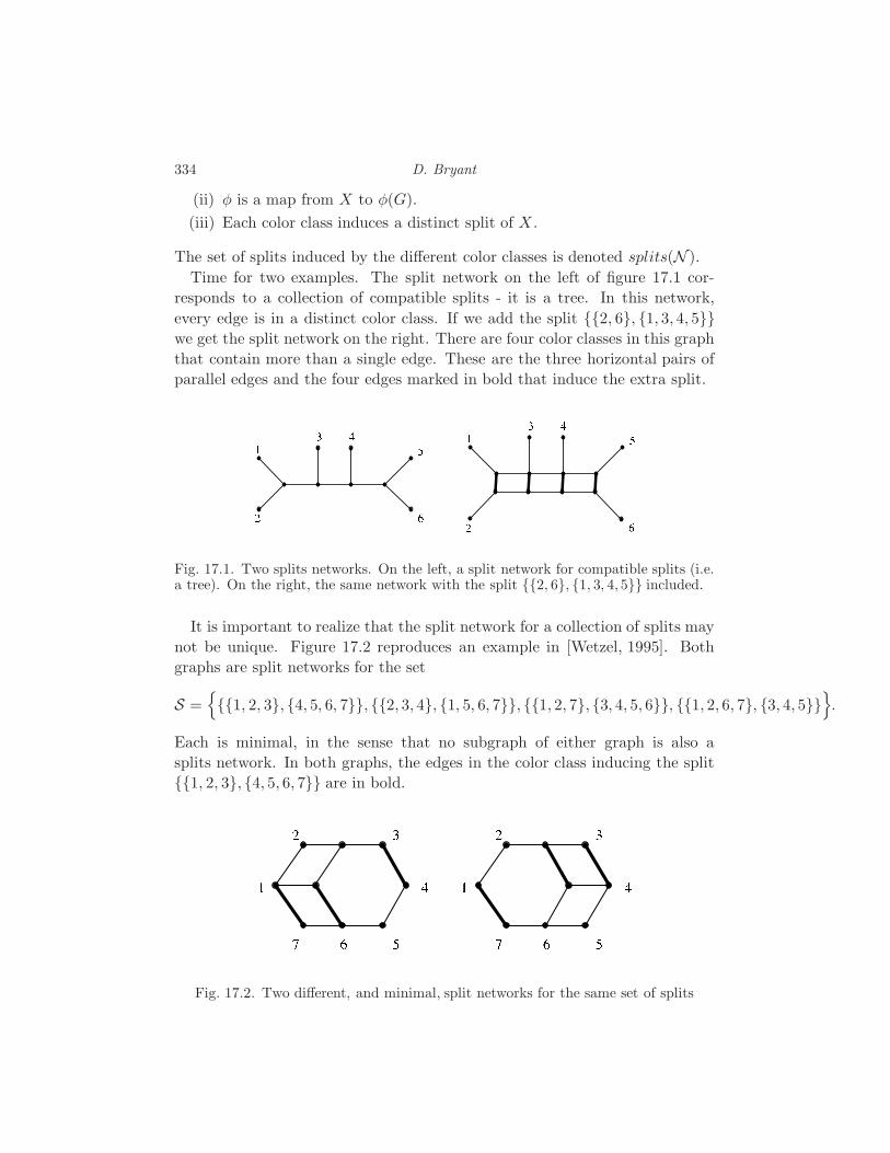
334 D. Bryant
(ii) φ is a map from X to φ(G).
(iii) Each color class induces a distinct split of X .
The set of splits induced by the different color classes is denoted splits(N ).
Time for two examples. The split network on the left of figure 17.1 cor-
responds to a collection of compatible splits - it is a tree. In this network,
every edge is in a distinct color class. If we add the split 2, 6, 1, 3, 4, 5we get the split network on the right. There are four color classes in this graph
that contain more than a single edge. These are the three horizontal pairs of
parallel edges and the four edges marked in bold that induce the extra split.123 4 56
12
3 4 56
Fig. 17.1. Two splits networks. On the left, a split network for compatible splits (i.e.a tree). On the right, the same network with the split 2, 6, 1, 3, 4, 5 included.
It is important to realize that the split network for a collection of splits may
not be unique. Figure 17.2 reproduces an example in [Wetzel, 1995]. Both
graphs are split networks for the set
S =1, 2, 3, 4, 5, 6, 7, 2, 3, 4, 1, 5, 6, 7, 1, 2, 7, 3, 4, 5, 6, 1, 2, 6, 7, 3, 4, 5
.
Each is minimal, in the sense that no subgraph of either graph is also a
splits network. In both graphs, the edges in the color class inducing the split
1, 2, 3, 4, 5, 6, 7 are in bold.
1 2 3 4567 1 2 3 4567Fig. 17.2. Two different, and minimal, split networks for the same set of splits
Extending Tree Models to Split Networks 335
17.3 Distance based models for trees and splits graphs
In molecular phylogenetics, the length of an edge in a tree is typically measured
in terms of the average (or expected) number of mutations that occurred, per
site, along that edge. The evolutionary distance between two sequences equals
the sum of the lengths of the edges along the unique path the connects them
in the unknown ‘true’ phylogeny. There is a host of methods for estimating
the evolutionary distance starting from the sequences alone. These form the
basis of distance based approaches to phylogenetics.
The oldest statistical methods for phylogenetics use models of how evo-
lutionary distances estimated from pairwise comparisons of sequences differ
from the true evolutionary distances (or phyletic distances) in the true, but
unknown, phylogenetic tree [Cavalli-Sforza and Edwards, 1967, Farris, 1972,
Bulmer, 1991]. It is assumed that the pairwise estimates were distributed,
at least approximately, according to a multi-variate normal density centered
on the true distances. The variance-covariance matrix for the density, here
denoted by V , can be estimated from the data [Bulmer, 1991, Susko, 2003],
though early papers used a diagonal matrix, or the identity, for V .
Once we have a variance covariance matrix, and the observed distances, we
can begin maximum likelihood estimation of the true distances δT , from which
we can construct the maximum likelihood tree. Note that the term maximum
likelihood here refers only to our approximate distance based model, not to the
maximum likelihood estimation introduced by Felsenstein [Felsenstein, 1981].
The maximum likelihood estimator is the tree metric δT that maximizes the
likelihood function
L(δT ) = Φ(n2)
(d− δT |V )
where Φm is the probability density function for them dimensional multivariate
normal:
Φm(x|V ) =1
(2π)m2
√det(V )
e−12 xT V −1x.
Equivalently, we can minimize the least squares residue∑
w<x
∑
y<z
(δT (w, x)− d(w, x)
)V−1
(wx)(yz)
(δT (y, z)− d(y, z)
).
In either formulation, the optimization is carried out over all tree metrics in
TX , the space of X-trees (Chapter 2).
We can describe tree metrics in terms of linear combinations of split metrics.
The split metric for a split A,B is the pseudo-metric on X given by
δA,B(x, y) =
0 if x, y ⊆ A or x, y ⊆ B;
1 otherwise.

336 D. Bryant
Let wA,B denote the length of the edge associated to a split A,B ∈splits(T ). Then
δT =∑
A,B∈splits(T )
wA,BδA,B. (17.2)
This formulation is used when we want to estimate edge lengths on a fixed
topology.
Equation (17.2) generalizes immediately to split networks. Suppose that the
lengths of the edges in a split network N are given by the split weights wA,B.
Hence, all edges in the same color class have the same length. The distance
between two labeled vertices x, y is the length of the shortest path between
them, which in turn equals the sum of the weights of the splits separating x
and y. We can therefore define a network metric N by
δN =∑
A,B∈splits(N )
wA,BδA,B.
The statistical model for distances from splits networks then works exactly
as it did for phylogenetic trees. We assume that the observed distances d are
distributed according to a multi-variate normal centered on the network metric
δN . The covariance matrix can be estimated using the non-parametric method
of Susko [Susko, 2003]. The likelihood of a network metric δN is, as before,
given by L(δN ) = Φ(n2)
(d− dN ).
We immediately come across the problem of identifiability. Phylogenetic
trees, together with their edge lengths, are determined uniquely from their
tree metrics. The same does not apply for network distances. The split met-
rics δA,B associated to splits of a network will not, in general, be linearly
independent.
In practice, identifiability has not been too much of a problem. Split de-
composition produces weakly compatible collections of splits. These have lin-
early independent and are uniquely determined from their network metrics
[Bandelt and Dress, 1992]. Neighbor-Net produces networks based on circular
collections of splits which, as a subclass of weakly compatible splits, are also
uniquely determined from their network metrics.
However the most important shortcoming of distance based methods, for
either trees of networks, is that they lack the statistical efficiency of likelihood
methods based on full stochastic models (see, e.g. Felsenstein [Felsenstein, 2003]).
When we estimate distances from pair-wise sequence comparisons we are ef-
fectively ignoring the joint probabilities of larger sets of sequences. What we
gain in speed, we lose in accuracy.

Extending Tree Models to Split Networks 337
17.4 A graphical model on a splits network?
The Markov model for trees outlined in Chapter 2 and Chapter 4 is just
a special case in a general class of graphical models (Section 1.5). Given
the vast literature on graphical models, it seems that the logical generaliza-
tion of the hidden tree model would be a graphical model defined on the
splits network. This was the approach taken by [Strimmer and Moulton, 2000,
Strimmer et al., 2001]. We review this approach here, and point out why it
doesn’t really work.
Let N be a splits network. The first step is to choose a root and direct all
edges away from the root (Figure 17.3). We now can apply a directed graphical
model. The probability that a node is assigned a particular state depends on
the states assigned to its parents: Strimmer and Moulton suggest several ways
that this may be done.
12 3
4567
Fig. 17.3. Edge directions induced by placing the root at the white vertex.
There are several problems with this general approach. Firstly, the prob-
ability of observing the data changes for different positions of the root, even
when the mutation process is a time reversible model. It was claimed that this
permitted estimation of the root, but there is no indication that the differences
in distributions corresponded to any evolutionary phenomenon.
Secondly, different split networks for the same set of splits give different
pattern probabilities, even though the networks represent exactly the same
information.
Thirdly, the internal nodes in split networks do not represent hypothetical
ancestors, they are products of an embedding in a hypercube.
Strimmer et al. eventually concluded that split networks may not provide
a suitable underlying graph for a stochastic network [Strimmer et al., 2001].
It is true that graphical model technology can not be applied ‘straight-off-
338 D. Bryant
the-shelf’ to split networks. We need to be more sensitive to the particular
properties of split networks. In the following section we will develop a model
for split networks that avoids the problems encountered in the graphical model
approach. The downside, however, is that we must first restrict ourselves to a
special class of mutation models: group based models.
17.5 Group based mutation models
A mutation model on state space 1, 2, . . . , r is said to be a group based model
if there exists an abelian group G with elements g1, . . . , gr and a function
ψ : G → ℜ such that the instantaneous rate matrix Q satisfies
Qij = ψ(gj − gi)
for all i, j. The group operation on G is denoted using addition and we will
use 0 for the identity element.
Let f be a function from G to the set of complex numbers C such that
f(g + g′) = f(g)f(g′) for all g, g′ ∈ G. Then f is a homomorphism from G to
C. The set of these homomorphisms forms a group G that is isomorphic to G.
We label the elements of G so that the map g → g taking g ∈ G to g ∈ G is an
isomorphism. If g = 0 then g is the function taking every element of G to 1.
Lemma 17.1 Suppose that g, h, h′ ∈ G, a ∈ Z. Then we have the following
identities:
g(−h) = g(h);
g(h+ h′) = g(h)g(h′);
(h+ h′)(g) = h(g)h′(g);
ag(h) = g(ah);
∑
h∈G
g(h) =
|G| if g = h;
0 otherwise.
Proof See, for example, [Korner, 1989].
Some indexing conventions will make our life easier. Since the elements of
G are in one to one correspondence with 1, 2, . . . , r we will index Q and P (t)
by group elements. So Qgigj is equivalent to Qij .
We start with some basic observations about group valued models.
Lemma 17.2 (i) The eigenvalues of Q are given by
λg =∑
h∈G
g(h)ψ(h).
Extending Tree Models to Split Networks 339
(ii) The transition probabilities are given by
Pgg′(t) =1
r
∑
h∈G
h(g′ − g)eλht.
(iii) The uniform distribution is a stationary distribution.
(iv) If the process is ergodic and time reversible then ψ(g) = ψ(−g) for all
g ∈ G.
Proof Define the r × r matrix K by Kij = gi(gj). Then
(KQ)gg′ =∑
h∈G
g(h)ψ(g′− h)
=∑
h∈G
g(g′ − h)ψ(h) [replacing h by g′ − h]
= g(g′)∑
h∈G
g(h)ψ(h)
= Kgg′λg.
Thus the rows of K are left-eigenvectors for Q. This proves (i). Let Λ be the
diagonal matrix with Λgg = λg. Then Q = K−1ΛK. By the orthogonality
property in Lemma 17.1 we have K−1 = 1|G|K
∗. Thus
Pgg′(t) = (eQt)gg′
=1
|G|(K∗eΛtK)gg′
=1
r
∑
h∈G
h(g)eλhth(g′)
=1
r
∑
h∈G
h(g′ − g)eλht
proving (ii). For (iii), observe that the first row of K gives a left-eigenvector
that is all ones. Finally, if the process is ergodic then the uniform distribution
is the unique stationary distribution. This, together with the assumption that
the process is time reversible, implies that both Q and P (t) are symmetric and
that ψ(g) = ψ(−g) for all g.
We define
φt(g) =1
r
∑
h∈G
h(g)eλht
so that Pgg′(t) = φt(g′ − g) for all g, g′ ∈ G and t ≥ 0.
340 D. Bryant
As an example, consider the case when r = 4. There are two (up to isomor-
phism) abelian groups on four elements, Z4 and Z2 × Z2. If G = Z4 then the
condition that ψ(g) = ψ(−g) implies that Q must have the form
Q =
−2a− b a b a
a −2a− b a b
b a −2a − b a
a b a −2a− b
so the mutation model is a sub-class of the K2P model (Chapter 4). If G =
Z2 × Z2 then we always have g = −g so there are three parameters available
for Q:
Q =
−a− b− c a b c
a −a − b− c c b
b c −a − b− c a
c b a −a − b− c
.
In this case, the mutation models are a subclass of Kimura’s three parameter
model [Kimura, 1981].
17.6 Group based models on trees and splits
Suppose that we have an ergodic, time reversible, group based mutation model
with state set Σ = 1, 2, . . . , r and abelian group G, where Qij = ψ(gj − gi)
for all i, j. Let P (t) = eQt denote the corresponding transition probabilities.
Let T be a phylogenetic tree with n leaves. We use te = tkl to denote the
length of an edge e = kl ∈ E(T ). In terms of the tree model of Chapter 2,
θkl = P (tkl) for all kl ∈ E(T ).
Lemma 17.3 Let σ be a map from N (T ) to Σ. For each edge e = kl define
xe = gσl− gσk
. Then
pσ =1
r
∏
e∈E(T )
φ(xe).
Extending Tree Models to Split Networks 341
Proof By Lemma 17.2 the mutation model has a uniform stationary distribu-
tion. We can therefore apply (1.53), giving
pσ =1
|Σ|∏
kl∈E(T )
θklσkσl
=1
r
∏
kl∈E(T )
φtkl(gσl
− gσk)
=1
r
∏
e∈E(T )
φte(xe).
Let χ be a map from the leaves of T to Σ. We say that σ : N (T ) → Σ extends
χ if σi = χi for all leaves i. Under the hidden tree model the probability of
observing χ is defined
pχ =∑
σ:σ extends χ
pσ.
Suppose that E(T ) = e1, e2, . . . , eq, let Ak, Bk be the split associated to
edge k and let A be the (n − 1)× q matrix defined by
(A)ik =
1 i and n are on opposite sides of Ak, Bk0 otherwise.
(17.3)
The next observation is crucial.
Theorem 17.4 Define the vector y = y[χ] ∈ Gn−1 by yi = χi − χn. Then
pχ =∑
x:Ax=yx∈Gq
∏
e∈E(T )
φte(xe). (17.4)
Proof Suppose that x is defined from σ as in Lemma 17.3. We prove that
Ax = y if and only if σ extends χ, so that the result follows from Lemma 17.3.
For each leaf i, let Ei be the edges on the path from leaf n to leaf i. We will
assume that T is rooted at leaf n, so all edges in Ei are directed away from n.
Then
(Ax)i =∑
kl∈Ei
xkl
=∑
kl∈Ei
(gσl− gσk
)
= gσi − gσn .
342 D. Bryant
Thus Ax = y if and only if gσi = χi for all leaves i, if and only if σ extends χ.
The importance of Theorem 17.4 so far as we are concerned is that pχ is not
expressed in terms of the tree structure: it is defined in terms of splits. We
can therefore generalize the definition of pattern probabilities to any collection
of splits.
Let N be a weighted split network with splits A1, B1, A2, B2, . . . , Aq, Bqand let tk be the length assigned to split Ak, Bk. Let A be the matrix de-
fined by Equation 17.3. The probability of a phylogenetic character χ given Nis then defined by
pχ =∑
x:Ax=yx∈Gq
q∏
k=1
φtk(xk). (17.5)
Astute readers will notice an uncanny similarity between (17.4) and (17.5).
Theorem 17.5 Let N be a weighted split network. If the splits of N are
compatible then the character probabilities correspond to exactly those given by
the tree based model.
We can rephrase this model in terms of graphical models on the splits net-
work. We say that a map σ : V (N ) → Σ is concordant if σl − σk = σj − σi
for all pairs of edges ij, kl ∈ E(N ) in the same color class. The probability of
a map σ is just the product of Pσkσl(tkl) over all edges kl ∈ E(T ), where tkl
is the length of the edge. We then have that pχ equals the probability that a
map σ extends χ, conditional on σ being concordant.
17.7 A Fourier calculus for split networks
Szekely et al. [Szekely et al., 1993] describe a Fourier calculus on evolution-
ary trees that generalizes the Hadamard transform of [Hendy and Penny, 1989,
Steel et al., 1992]. Using their approach, we can take the observed character
frequencies, apply a transformation, and obtain a vector of values from which
we can read off the support for different splits. They show that if the ob-
served character frequencies correspond exactly to the character probabilities
determined by some phylogenetic tree then the split supports will correspond
exactly to the splits and branch lengths in the phylogenetic tree. Conversely,
the inverse transformation gives a single formula for the character probabilities
in any tree.
This theory generalizes seamlessly from trees to split networks—in fact so
seamlessly that the proofs of [Szekely et al., 1993] require almost no modifi-
cations to establish the general case. Their approach was prove that their
Extending Tree Models to Split Networks 343
transform worked when applied to character probabilities from a tree. The
correctness of the inverse formula then followed by applying a Fourier trans-
formation. In this section we will prove the same results but working in the
opposite direction. We show that, starting with weights on the splits, a sin-
gle invertible formula gives the character probabilities. Our rationale is that,
at some point in the future, we will need to generalize these results beyond
Abelian group models, and the elegant Fourier inversion formula may not exist
in this context.
First a little more algebra. For x, y ∈ Gm we define
y(x) =
m∏
i=1
yi(xi).
The set y : y ∈ Gm forms a group under multiplication that is isomorphic
to Gm.
The following can (and should) be proved directly using an elegant result in
algebra, but I could only come up with a low-technology proof.
Lemma 17.6 Suppose that z ∈ Gq and y ∈ Gn−1. Let A be an (n − 1) × q
integer matrix with linearly independent rows. Either∑
x∈Gq:Ax=y
z(x) = 0
or there is u ∈ Gn−1 such that z = ATu and so∑
x∈Gq:Ax=y
z(x) = rq−(n−1) z(u)
Proof Suppose that∑
x∈Gq :Ax=y z(x) 6= 0. For any v such that Av = 0 we
have∑
x∈Gq:Ax=y
z(x) =∑
x∈Gq:Ax=y
z(x+ v) = z(v)∑
x∈Gq:Ax=y
z(x)
so z(v) = 1.
For every x, y ∈ Gn−1 we have
Ax = Ay ⇔ A(x− y) = 0 ⇔ z(x− y) = 1 ⇔ z(x) = z(y).
We can thus define a map f : Gn−1 → C by setting f(Ax) = z(x) for all
x ∈ Gq. This is a homomorphism, since f(Ax+Ay) = f(A(x+y)) = z(x+y) =
z(x)z(y) = f(Ax)f(Ay). Thus there is u such that f = u and, for all x ∈ Gq,
z(x) = u(Ax). The result now follows by expanding u(Ax).
We will assume that N contains all the trivial splits i, X − i since

344 D. Bryant
these can be added and assigned weight zero. Let H be the matrix with rows
and columns indexed by Gn−1 and Hgg′ = g(g). Define the vector b by
bz =
ψ(h)tk if there is h ∈ G and k such that z = Aikh for all i
−∑v∈Gn−1−0 bv if z = 0
0 otherwise.
Theorem 17.7 Let y ∈ Gn−1 be the vector such that yi = gχn − gχi for all
leaves i. Then
pχ =[H−1 exp[Hb]
]y. (17.6)
Proof ¿From (17.5) we have
pχ =∑
x:Ax=yx∈Gq
q∏
k=1
φtk(xk)
=∑
x:Ax=yx∈Gq
q∏
k=1
1
r
∑
h∈G
h(xk)eλhtk
=1
rq
∑
x:Ax=yx∈Gq
∑
z∈Gq
q∏
k=1
zk(xk)eλzk
tk
=1
rq
∑
z∈Gq
∑
x:Ax=yx∈Gq
z(x)
exp
[q∑
k=1
λzktk
].
So far we have just applied the definitions, reversed a summation and product,
and regrouped. From Lemma 17.6 we get that z(x) = 0 unless z = ATu for
some u (the change from u to u is not a problem). Substituting in we obtain
pχ =1
rn−1
∑
u∈Gn−1
u(y)eβu
= H−1 exp[β]
Extending Tree Models to Split Networks 345
where
βu =
q∑
k=1
λ(AT u)ktk
=
q∑
k=1
∑
h∈G
ATuk(h)ψ(h)tk
=
q∑
k=1
∑
h∈G
u(ηkh)ψ(h)tk
=∑
v∈Gn−1
u(v)bv
= Hb.
We have proven, more or less, Theorem 6 of [Szekely et al., 1993] without
any reference to trees. In the special case that r = 2, (17.6) becomes the
classical Hadamard transform of [Hendy and Penny, 1989, Steel et al., 1992].
Note that the formula H−1 exp[Hb is invertible. This means that every
split network gives a different character distribution. We cannot recover split
networks from their distance metrics dN but we can recover them from their
character probabilities. A maximum likelihood estimator based on (17.6) will
be statistically consistent.
17.8 Discussion
We have discussed ways in which stochastic models for trees can be general-
ized to split networks. En route, we have rediscovered the Fourier calculus
approach of [Szekely et al., 1993]. This is comforting: Felsenstein describes
the Hadamard type approach as “one of the nicest applications of mathemat-
ics to phylogenies so far.” While we have not made a substantial mathematical
contribution to the theory, we have proposed a quite different way to look at
these methods.
For us, the Hadamard transform is useful because it gives character proba-
bilities for general collections of splits, not because it is invertible. A maximum
likelihood method, or Bayesian method, only requires a way to compute char-
acter probabilities. The transform taking probabilities to split weights is less
useful in this context, since it requires a huge number of parameters. If we use
the Hadamard as a statistical model we can optimize likelihood and restrict
the number of parameters appropriately.
One key problem remains. The constraint that we only use group based

346 D. Bryant
mutation models is too much of a restriction. For nucleotide data, and es-
pecially for protein data, a uniform stationary distribution is unrealistic. It
is reasonable to believe that some reasonable generalization of these results
exists for more general mutation models: after all there is no such restriction
on distance based methods. What exact form these generalizations will take
is, at the moment, anybody’s guess.
18
Small Trees and Generalized Neighbor-Joining
Mark Contois
Dan Levy
Direct reconstruction of phylogenetic trees by maximum likelihood methods is
computationally prohibitive for trees with many taxa; however, by computing
all trees for subsets of taxa of size m, we can attempt to infer the entire
tree. In particular, if m = 2, the traditional distance-based methods such as
neighbor-joining [Saitou and Nei, 1987] and UPGMA [Sneath and Sokal, 1973]
are applicable. Under distance-based methods, 2-leaf subtrees are completely
determined by the total length between the pairs of leaves. We extend this
idea to m leaves by defining the m-dissimilarity of a set R ∈(Xm
)as the total
length of the subtree spanning R. By building small subtrees of size m and
finding the total length, we can obtain an m-dissimilarity map on X . We will
define the Generalized Neighbor-Joining (GNJ) algorithm [Levy et al., 2004]
for obtaining a phylogenetic X-tree with edge lengths given an m-dissimilarity
map on X .
This algorithm is consistent: given an m-dissimilarity map DT that comes
from a tree T , GNJ returns the correct tree. However, in the case of data that
is “noisy”, e.g., when the observed dissimilarity map does not lie in the space of
X-trees, the accuracy of GNJ depends on the reliability of the subtree lengths.
Numerical methods may run into trouble when models are of high degree (1.3);
exact methods for computing subtrees, therefore, could only serve to improve
the accuracy of GNJ. One family of such methods consists of algorithms to
find critical points of the ML equations as discussed in chapter 15 and in
[Hosten et al., 2004]. We explore the results of this method for the Jukes-
Cantor DNA model on three taxa and conjecture that, for any 3-subtree, there
is at most one critical point yielding edge lengths that are positive and real.
18.1 From Alignments to Dissimilarity
Any method for phylogenetic tree reconstruction begins with a sequence align-
ment. Distance-based methods then proceed by comparing pairs of taxa from
347
348 M. Contois and D. Levy
this alignment to find the distances between them. Let X be the set of taxa
and(X
k
)the set of all subsets R ⊂ X such that |R| = k. Then
(X2
)is the set
of all pairs of taxa and D :(X
2
)→ R>0 assigns a distance to each pair of taxa.
We call D a dissimilarity map on X . Where there is no confusion, we will
write D(a, b) as D(a, b).
If a and b are taxa in X , we may compare their aligned sequences to find
the Jukes-Cantor corrected distance DJC(a, b). If the alignment has a length
of L and a and b differ in k places, then
DJC(a, b) = −3
4log
(1 − 4
3p
)(18.1)
where p = kL . It has been shown in 4.2 that DJC(a, b) is the maximum likeli-
hood branch length estimate of the alignment of a and b, with respect to the
JC model on the simple two-leaf tree. The conceit of distance-based meth-
ods is that the branch length estimate on the two-leaf tree is a good estimate
of the total path length from a to b in the maximum likelihood tree T on
X . Stated in the terms of section 2.4, distance based methods are effective
when DJC is close to δT , the tree metric on X induced by T . (Recall that
δT (a, b) =∑
e∈PablT (e), where Pab is the path from a to b in T and lT is the
length function associated to the edges of T .)
We can extend the notion of dissimilarity maps to subsets of X larger than
two. We define an m-dissimilarity map on X as a function D :(Xm
)→ R>0.
That is, D assigns a positive real value to every subset of X of size m. In
particular, a dissimilarity map is a 2-dissimilarity map. Again, where there
is no confusion, we will write D(x1, ..., xm) as D(x1, ..., xm). For a subset
R ⊆ X , we define [R] as the spanning subtree of R in T : [R] is the smallest
subtree of T containing R. For two leaves, a, b ∈ X , the path from a to b, Pab,
is equivalent to the spanning subtree [a, b].Just as we defined tree metrics induced by a tree T , we can define the m-
dissimilarity map induced by T , DTm :(Xm
)→ R>0 by
DTm(R) =
∑
e∈[R]
lT (e)
for R ⊂ X, |R| = m. DTm(R) is the sum of all the edge lengths in the spanning
subtree of R. We call DTm(R) the m-subtree length of [R]. Since Pab = [a, b],
DT2 (a, b) = δT (a, b), and the 2-dissimilarity map induced by T is a tree metric.
Just as we used the JC corrected distance to approximate δT , we can employ
analytical or numerical methods to find maximum likelihood estimates for the
total branch lengths of subtrees with m leaves. To find an approximate m-
dissimilarity map, D, for all R ∈(Xm
), we find the MLE tree for R and sum
Small Trees and Generalized Neighbor-Joining 349
the branch lengths:
D(R) =∑
e∈T (R)
lT (R)(e)
where T (R) is the MLE tree for R.
18.2 From Dissimilarity to Trees
The neighbor-joining algorithm and its variants are examples of methods that
take an approximate dissimilarity map and construct a “nearby” tree. Sim-
ilarly, we would like to define an algorithm that takes as its input an m-
dissimilarity map and constructs a “nearby” tree, and we would like this
method to be consistent: given an m-dissimilarity map DTm induced by a tree
T , our algorithm should return T .
The crux of our method is the construction of a 2-dissimilarity map SD from
the m-dissimilarity map D. In the case that D is induced by a tree T , then
SD will be the tree metric induced by a tree T ′. Further, T ′ is isomorphic to a
contraction of certain “deep” edges, E>n−m(T ), of T . If |X | > 2m− 1, then T
and T ′ are topologically equivalent. Further, there exists an invertible linear
map from edge lengths of T to the edge lengths of T ′.
The deletion of an edge e in T divides T into two subtrees T1(e) and T2(e).
If L(T1(e)) and L(T2(e)) are the leaves in each subtree, then we define the
depth of e, d(e) by
d(e) = min(|L(T1(e))|, |L(T2(e))|).Observe that the pendant edges are exactly those edges of depth 1, and, if T
has n leaves, then d(e) ≤ n2 for any e ∈ E(T ). We define E>k(T ) = e ∈ E :
d(e) > k. For example, E>1(T ) is all the interior edges of T .
For any edge e in T , we may contract e by deleting the edge and identifying
its vertices. We write the resulting tree as T/e and for a set of edges E ′,
the contraction of each edge in that set is denoted as T/E ′. For example,
T/E>1(T ) contracts all interior edges and has the star topology (figure 18.1).
We may now state our claim explicitly:
Theorem 18.1 Let D be an m-dissimilarity map on a set X of size n. We
define
SD(i, j) =∑
R∈(X\i,jm−2 )
D(i, j, R). (18.2)
If D = DTm then SD = DT ′
and T ′ is isomorphic to T/E>n−m. Further, there
exists an invertible linear transformation between the interior edge lengths of
T ′ to T/E>n−m. If E>n−m is empty, then there is also an invertible linear

350 M. Contois and D. Levy
Fig. 18.1. In the center, we have a tree T surrounded by T/E>k for k = 11, 4, 2, and 1starting at the top left and proceeding clockwise. The red circle represents the vertexto which the edges of E>k have collapsed. Notice that T has 24 leaves and so E>12 = ∅and T/E>12 = T .
transformation between the pendant edges; otherwise, the pendant edges may
not be determined uniquely.
Observe that for a phylogenetic X-tree with edge lengths, T , any linear com-
bination of the m-subtree lengths is a linear combination of the edge lengths
lT (e) in the tree. This is because DTm(R) =
∑e∈[R] lT (e); i.e. every m-subtree
length is the sum of the edge lengths in the spanning subtree. For a linear
function on the m-subtree lengths F : R(nm) → R, let vF (e) denote the coeffi-
cient of lT (e) in F . For instance, vS(i,j)(e) denotes the coefficient of lT (e) in
S(i, j). Note that vF+G(e) = vF (e) + vG(e). We will also use the notation
Li(e) to denote the set of leaves in the component of T \ e that contains leaf i.
Lemma 18.2 Given a pair of leaves a, b and any edge e we have
vS(a,b)(e) =
(n−2m−2
)e ∈ Pab;
(n−2m−2
)−(|La(e)|−2
m−2
)e /∈ Pab.
Proof If e is on the path from a to b, then it will be included in all the subtrees

Small Trees and Generalized Neighbor-Joining 351
[a, b, Y ]. If e is not on the the path from a to b, then the only way it will be
excluded is if all the other leaves fall on the a side of e (which is the same as
the b side); that is, if Y ⊂ La(e) \ a, b. There are(|La(e)|−2
m−2
)such sets.
Lemma 18.3 Given a quartet (a1, a2; a3, a4) in T with interior vertices b1 and
b2 (figure 18.2),
vS(a1,a2)+S(a3,a4)(e) =
2(n−2m−2
)−(n−|Lai (e)|−2
m−2
)e ∈ Paib⌈i/2⌉
;
2(
n−2m−2
)−(|La1(e)|−2
m−2
)−(|La3(e)|−2
m−2
)e ∈ Pb1b2 ;
2(
n−2m−2
)− 2(|La1(e)|−2
m−2
)e /∈ [a1, a2, a3, a4].
vS(a1,a3)+S(a2,a4)(e) =
2(
n−2m−2
)−(n−|Lai (e)|−2
m−2
)e ∈ Paib⌈i/2⌉
;
2(
n−2m−2
)e ∈ Pb1b2 ;
2(n−2m−2
)− 2(|La1(e)|−2
m−2
)e /∈ [a1, a2, a3, a4].
and
vS(a1,a4)+S(a2,a3) = vS(a1,a3)+S(a2,a4)
a1
a2
b1 b2
a3
a4
Fig. 18.2. A quartet (a1, a2; a3, a4)
Proof We use the fact that vS(a1,a2)+S(a3,a4) = vS(a1,a2) + vS(a3,a4) and apply
the previous lemma. We also note that for e /∈ [a1, a2, a3, a4], La1(e) = Lai(e)
for all i.
Corollary 18.4 For a quartet (a1, a2; a3, a4), we define
S(a1, a2; a3, a4) = S(a1, a2) + S(a3, a4)− S(a1, a3)− S(a2, a4).

352 M. Contois and D. Levy
Then,
vS(a1,a2;a3,a4)(e) =
−(|La1(e)|−2
m−2
)−(n−|La1 (e)|−2
m−2
)e ∈ Pb1b2 ;
0 otherwise.
Corollary 18.4 implies that S satisfies the four-point condition (as discussed
in section 2.4 and theorem 2.35) although it may be that vS(a1a2;a3a4)(e) = 0
which means that the edge e has been contracted in T ′. In particular, this
happens when |La1(e)| < m and n − |La1(e)| < m which is equivalent to
d(e) > n −m. So for any quartet (a1, a2; a3, a4), if the splitting path contains
at least one edge e such that d(e) ≤ n − m, then T ′ has the same quartet.
However, if every edge in the splitting path has d(e) > n −m, then T ′ does
not contain that quartet. Consequently, T ′ is isomorphic to T/E>n−m.
It remains to show that there is an invertible linear map between the edge
lengths in the T ′ and T/E>n−m:
Lemma 18.5 If e is an internal edge of T/E>n−m with e′ the corresponding
edge in T ′ then
lT ′(e′) =1
2
((|La(e)| − 2
m− 2
)+
(|Lc(e)| − 2
m− 2
))lT (e)
where a is a leaf in one component of T − e and c a leaf in the other.
Proof Since e is an internal edge, we may choose a, b, c and d such that e is
the only edge on the splitting path of (a, b; c, d) (figure 18.3). Then
lT ′(e′) =1
2S(a, b; c, d)
=1
2
((|La(e)| − 2
m− 2
)+
(|Lc(e)| − 2
m− 2
))lT (e)
=1
2
((d(e)− 2
m− 2
)+
(n− d(e)− 2
m− 2
))lT (e).
Corollary 18.6
lT (e) =2lT ′(e′)((
d(e)−2m−2
)+(n−d(e)−2
m−2
))
which is well defined if d(e) ≤ n −m.
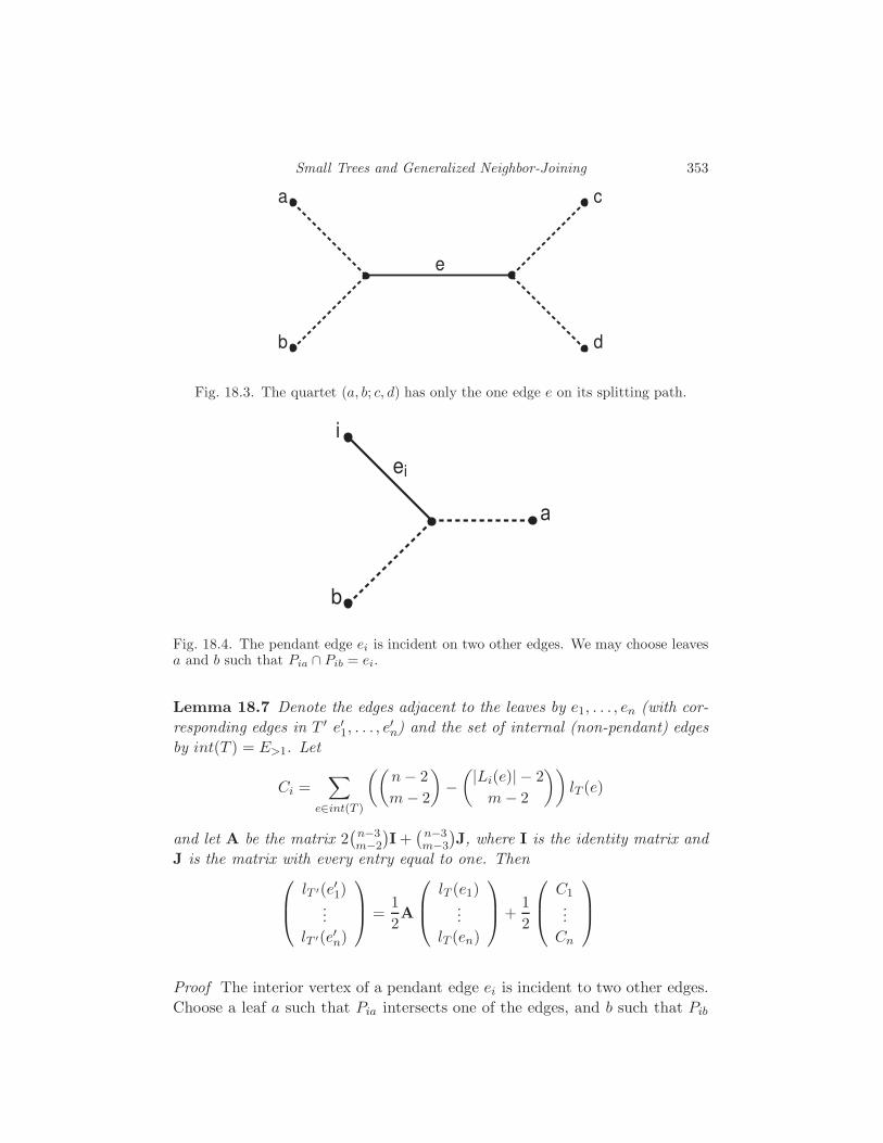
Small Trees and Generalized Neighbor-Joining 353
a
b
c
d
e
Fig. 18.3. The quartet (a, b; c, d) has only the one edge e on its splitting path.
i
b
e i
a
Fig. 18.4. The pendant edge ei is incident on two other edges. We may choose leavesa and b such that Pia ∩ Pib = ei.
Lemma 18.7 Denote the edges adjacent to the leaves by e1, . . . , en (with cor-
responding edges in T ′ e′1, . . . , e′n) and the set of internal (non-pendant) edges
by int(T ) = E>1. Let
Ci =∑
e∈int(T )
((n− 2
m− 2
)−(|Li(e)| − 2
m− 2
))lT (e)
and let A be the matrix 2(
n−3m−2
)I +
(n−3m−3
)J, where I is the identity matrix and
J is the matrix with every entry equal to one. Then
lT ′(e′1)...
lT ′(e′n)
=
1
2A
lT (e1)...
lT (en)
+
1
2
C1...
Cn
Proof The interior vertex of a pendant edge ei is incident to two other edges.
Choose a leaf a such that Pia intersects one of the edges, and b such that Pib
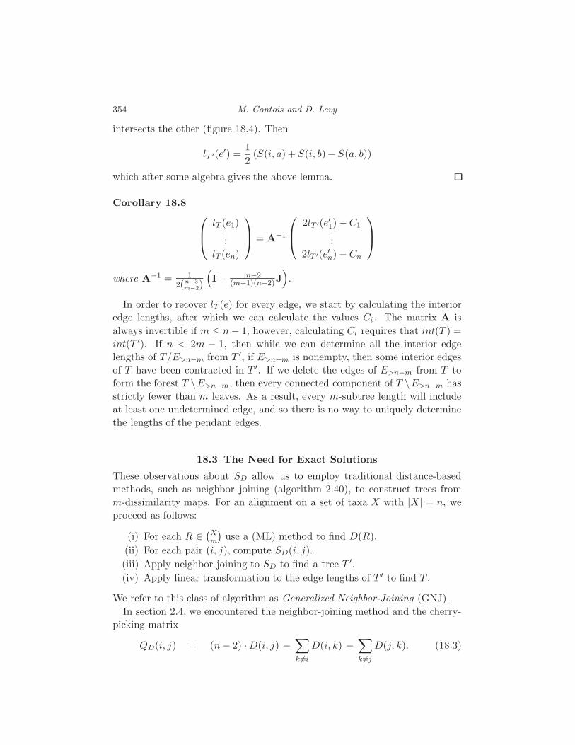
354 M. Contois and D. Levy
intersects the other (figure 18.4). Then
lT ′(e′) =1
2(S(i, a) + S(i, b)− S(a, b))
which after some algebra gives the above lemma.
Corollary 18.8
lT (e1)...
lT (en)
= A−1
2lT ′(e′1) −C1...
2lT ′(e′n) −Cn
where A−1 = 12(n−3
m−2)
(I − m−2
(m−1)(n−2)J).
In order to recover lT (e) for every edge, we start by calculating the interior
edge lengths, after which we can calculate the values Ci. The matrix A is
always invertible if m ≤ n − 1; however, calculating Ci requires that int(T ) =
int(T ′). If n < 2m − 1, then while we can determine all the interior edge
lengths of T/E>n−m from T ′, if E>n−m is nonempty, then some interior edges
of T have been contracted in T ′. If we delete the edges of E>n−m from T to
form the forest T \E>n−m, then every connected component of T \E>n−m has
strictly fewer than m leaves. As a result, every m-subtree length will include
at least one undetermined edge, and so there is no way to uniquely determine
the lengths of the pendant edges.
18.3 The Need for Exact Solutions
These observations about SD allow us to employ traditional distance-based
methods, such as neighbor joining (algorithm 2.40), to construct trees from
m-dissimilarity maps. For an alignment on a set of taxa X with |X | = n, we
proceed as follows:
(i) For each R ∈(Xm
)use a (ML) method to find D(R).
(ii) For each pair (i, j), compute SD(i, j).
(iii) Apply neighbor joining to SD to find a tree T ′.
(iv) Apply linear transformation to the edge lengths of T ′ to find T .
We refer to this class of algorithm as Generalized Neighbor-Joining (GNJ).
In section 2.4, we encountered the neighbor-joining method and the cherry-
picking matrix
QD(i, j) = (n− 2) ·D(i, j) −∑
k 6=i
D(i, k) −∑
k 6=j
D(j, k). (18.3)

Small Trees and Generalized Neighbor-Joining 355
If D is a tree metric for a tree T , then the minimum entry QD(x, y) identifies
x, y as a cherry in T . We also encountered the quartet split length
wD(i, j; k, l) =1
4[2D(i, j)+ 2D(k, l)−D(i, k)−D(i, l)−D(j, k)−D(j, l)]
which was instrumental in constructing an analogue to the cherry picking ma-
trix. Here, we will see that it also plays a crucial rule in describing the effect
of agglomeration on the cherry picking matrix.
Having chosen a pair x, y that minimizes QD, the neighbor joining algo-
rithm proceeds to agglomerate x and y to a single vertex z. We form a new
set X ′ = X \x, y∪z and define D′ as a dissimilarity map on X ′ such that,
for k, l ∈ X ′ \ z,
D′(z, k) =1
2[D(x, k) +D(y, k)−D(x, y)],
D′(k, l) = D(k, l).
A brief computation allows us to explicitly relate the agglomeration update to
the cherry-picking matrix. Specifically:
QD′(z, k) =1
2[QD(x, k) +QD(y, k)] + 2D(x, y),
QD′(k, l) = QD(k, l) + 2wD(x, y; k, l)+ 2D(x, y)
where QD′ is the (n− 1)× (n− 1) cherry-picking matrix after agglomeration.
Given a 2-dissimilarity map D, we may construct a 3-dissimilarity map in-
duced by D as follows:
D3(i, j, k) =1
2[D(i, j) +D(i, k) +D(j, k)]. (18.4)
Theorem 18.9 Given D :(X
2
)→ R>0, define D3 as in equation (18.4). If
we let S = SD3 , then QS is related to QD by an affine transformation. If S ′
and D′ are the 2-dissimilarity maps on X ′ after agglomeration of S and D
respectively, then QS′ and QD′ are also related by an affine transformation.
Proof We first note that
S(i, j) =∑
x∈X\i,j
D3(i, j, x)
=1
2
∑
x∈X\i,j
D(i, j)+D(i, x) +D(j, x)
=1
2[(n− 4)D(i, j)+
∑
x∈X\i
D(i, x) +∑
x∈X\j
D(j, x)]. (18.5)

356 M. Contois and D. Levy
We substitute (18.5) into the cherry picking equation (18.3) and find that
QS =n− 4
2QD − 2T,
where T =∑D(x, y) over all x, y ∈
(X2
).
To compute the effect on the update function, we agglomerate x and y to a
vertex z as above. We first note that
wS(i, j; k, l) =n − 4
2wD(i, j; k, l).
Applying this to the update function (18.4), we obtain
QS′ =n− 4
2QD′ − 2T +
∑
i∈X\x
D(i, x) +∑
y∈X\x
D(i, y).
Corollary 18.10 Given a 2-dissimilarity map D and induced 3-dissimilarity
map D3, neighbor-joining applied to D is equivalent to GNJ applied to D3.
Corollary 18.10 provides a means for comparing GNJ with traditional neighbor-
joining. In particular, given an MLE method for generating trees on alignments
of three taxa, we may compare its fidelity to the true total length with the fi-
delity of the 3-dissimilarity map induced by neighbor-joining’s 2-dissimilarity
map.
To this end, we compared the HKS method applied to Jukes-Cantor claw
trees (described in the following section) with the 3-dissimilarity map D3 con-
structed from Jukes-Cantor corrected 2-distances (as in equation 18.1). We
used seq-gen [Rambaut and Grassly, 1997] to generate pseudorandom align-
ments of triplets evolved from the Jukes-Cantor DNA model (α = 14 ) on four
different tree shapes over a range of total tree lengths. The total lengths varied
from .125 to 7 and for each total length and each tree shape, we generated 100
alignments of length 500. Figure 18.5 shows that as the total length increases,
HKS generated values, are, on average, closer to the true value than those
generated from the Jukes-Cantor corrected 2-distance.
We may infer from this and corollary 18.10 that generalized neighbor-joining
with the HKS claw tree will be more accurate than neighbor-joining with
Jukes-Cantor corrected distances, particularly in trees with large pairwise dis-
tances. Experiments coupling GNJ with fastDNAml, a numerical approxima-
tion method, show an improvement over traditional neighbor-joining [Levy et al., 2004].
If conjecture 18.12 is true, then methods such as fastDNAml which locate a
biologically meaningful local maxima, will be assured to have found the only
global maximum for 3-leaf trees, and therefore, are commensurate with a global
maxima method such as HKS.
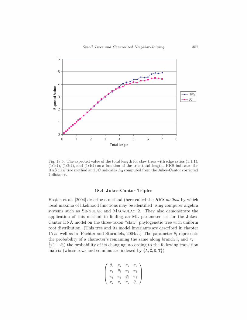
Small Trees and Generalized Neighbor-Joining 357
Fig. 18.5. The expected value of the total length for claw trees with edge ratios (1:1:1),(1:1:4), (1:2:4), and (1:4:4) as a function of the true total length. HKS indicates theHKS claw tree method and JC indicatesD3 computed from the Jukes-Cantor corrected2-distance.
18.4 Jukes-Cantor Triples
Hosten et al. [2004] describe a method (here called the HKS method by which
local maxima of likelihood functions may be identified using computer algebra
systems such as Singular and Macaulay 2. They also demonstrate the
application of this method to finding an ML parameter set for the Jukes-
Cantor DNA model on the three-taxon “claw” phylogenetic tree with uniform
root distribution. (This tree and its model invariants are described in chapter
15 as well as in [Pachter and Sturmfels, 2004a].) The parameter θi represents
the probability of a character’s remaining the same along branch i, and πi =13 (1− θi) the probability of its changing, according to the following transition
matrix (whose rows and columns are indexed by A, C, G, T):
θi πi πi πi
πi θi πi πi
πi πi θi πi
πi πi πi θi

358 M. Contois and D. Levy
We define the members of K = [123], [dis], [12], [13], [23] to be equivalence
classes of observed characters at homologous loci for our three taxa: [123]
indicates that all three characters are identical, and [dis] that all three are
distinct; [12] corresponds to identical characters at taxa 1 and 2 and a different
character at taxon 3; and so on. As described in Chapter 1, an observation here
is just a vector u = (u123, udis , u12, u13, u23) generated by tallying character
similarities over some number of loci.
The probability of making an observation in class k at a given locus is
denoted by pk. For the claw tree, we may write down each of these as a
trilinear form in θ1, θ2, θ3, π1, π2, π3:
p123 = θ1θ2θ3 + 3π1π2π3
pdis = 6θ1π2π3 + 6π1θ2π3 + 6π1π2θ3 + 6π1π2π3
p12 = 3θ1θ2π3 + 3π1π2θ3 + 6π1π2π3
p13 = 3θ1π2θ3 + 3π1θ2π3 + 6π1π2π3
p23 = 3π1θ2θ3 + 3θ1π2π3 + 6π1π2π3
Our wish, as the reader may have anticipated, is to find a parameter θ =
(θ1, θ2, θ3) that maximizes the likelihood function L(θ) =∏
k∈K pukk , or equiv-
alently the log-likelihood function ℓ(θ) =∑
k∈K uk log pk, given an observation
u.
Algebraic statistical methods, including HKS, tend to operate in vector
spaces of arbitrary dimension over algebraically closed fields such as C. For
many problems susceptible to ML methods, there is an obvious motivation to
constrain the solution set to a region (or regions) of the parameter space corre-
sponding to inputs that are in some sense “reasonable” or “meaningful”—this
has already been seen in examples such as 1.6, where only parameters lying in
the preimage of the probability simplex are admissible.
Specifically, for phylogenetic tree models it is natural to define the following
restricted parameter space:
Definition 18.11 Given an algebraic statistical model of a phylogenetic tree
T , a biologically meaningful parameter for the model is a parameter θ ∈ Θ ⊂ Rd
that induces a tree in which all branch lengths are nonnegative real.
In the case of the claw tree, branch lengths may be determined from tran-
sition probabilities by the Jukes-Cantor corrected distance map as given in
equation 18.1 (the transition probability p there is our θi). Now consider the
inverse map:
θi =1 + 3e−4bi/3
4(18.6)
Small Trees and Generalized Neighbor-Joining 359
where bi is the length of branch i. Note that θi ∈ R if and only if Im(bi) ∈3πn/4 | n ∈ Z; when bi is real, branch lengths in [0,∞) go to θi’s in ( 1
4 , 1].
On this tree, therefore, a biologically meaningful parameterization is one in
which 14 < θ1, θ2, θ3 ≤ 1.
We applied the HKS algorithm, using Maple and Singular code due to Gar-
cia and Hosten, to find local maxima of the likelihood function for this model,
and found that, given some 20,000 observation vectors—half with independent
randomly generated components and half derived from seq-gen alignments
—at most one biologically meaningful solution was found for each observation.
Conjecture 18.12 For any observation (uk), the Jukes-Cantor DNA claw
tree model admits at most one local maximum (pk) that gives a biologically
meaningful parameterization θ.
This conjecture, if true, would have a number of interesting consequences:
even if approximate numerical methods are used to target local maxima of the
likelihood function, we could be assured that any maximum occurring in the
biologically meaningful region Θ = (14 , 1]3 was unique. Identifying bounds on
the number of biologically meaningful ML solutions for this and other models
promises to be a rich area of inquiry.
19
Tree Construction Using Singular ValueDecomposition
Nicholas Eriksson
We present a new, statistically consistent algorithm for phylogenetic tree con-
struction that uses the algebraic theory of statistical models (as developed in
Chapters 1 and 3). Our basic tool is the Singular Value Decomposition (SVD)
from numerical linear algebra.
Starting with an alignment of n species, we show that the SVD allows us
to quickly decide whether a split of the species occurs in their phylogenetic
tree, assuming only that evolution follows a tree Markov model. Using this
fact, we have developed an algorithm (jointly with Sagi Snir) to construct a
phylogenetic tree by computing only n2 SVD’s.
We have implemented this algorithm using the SVDLIBC library† and have
done extensive testing with simulated and real data. The algorithm is very
fast in practice on trees with 20-30 taxa.
We begin by describing the general Markov model and then show how to
flatten the joint probability distribution along a partition of the leaves in the
tree. We give rank conditions for the resulting matrix; notably, we give a set
of new rank conditions that are satisfied by non-splits in the tree. Armed with
these rank conditions, we show how to use the SVD to calculate how close a
matrix is to a certain rank and present the tree building algorithm. Finally, we
give experimental results on the behavior of the algorithm with both simulated
and real-life (ENCODE) data.
19.1 The General Markov Model
We assume that evolution follows a tree Markov model, as introduced in Sec-
tion 1.4, with evolution acting independently at different sites of the genome.
We do not assume that the transition matrices for the model are stochastic.
Furthermore, we do not assume the existence of a global rate matrix (as in
Section 4.5).
† Available at http://tedlab.mit.edu/∼dr/SVDLIBC/
360
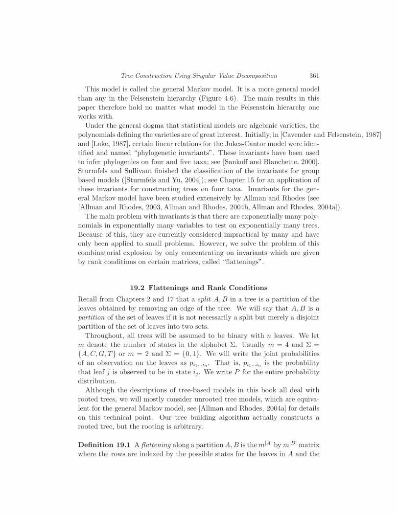
Tree Construction Using Singular Value Decomposition 361
This model is called the general Markov model. It is a more general model
than any in the Felsenstein hierarchy (Figure 4.6). The main results in this
paper therefore hold no matter what model in the Felsenstein hierarchy one
works with.
Under the general dogma that statistical models are algebraic varieties, the
polynomials defining the varieties are of great interest. Initially, in [Cavender and Felsenstein, 1987]
and [Lake, 1987], certain linear relations for the Jukes-Cantor model were iden-
tified and named “phylogenetic invariants”. These invariants have been used
to infer phylogenies on four and five taxa; see [Sankoff and Blanchette, 2000].
Sturmfels and Sullivant finished the classification of the invariants for group
based models ([Sturmfels and Yu, 2004]); see Chapter 15 for an application of
these invariants for constructing trees on four taxa. Invariants for the gen-
eral Markov model have been studied extensively by Allman and Rhodes (see
[Allman and Rhodes, 2003, Allman and Rhodes, 2004b, Allman and Rhodes, 2004a]).
The main problem with invariants is that there are exponentially many poly-
nomials in exponentially many variables to test on exponentially many trees.
Because of this, they are currently considered impractical by many and have
only been applied to small problems. However, we solve the problem of this
combinatorial explosion by only concentrating on invariants which are given
by rank conditions on certain matrices, called “flattenings”.
19.2 Flattenings and Rank Conditions
Recall from Chapters 2 and 17 that a split A,B in a tree is a partition of the
leaves obtained by removing an edge of the tree. We will say that A,B is a
partition of the set of leaves if it is not necessarily a split but merely a disjoint
partition of the set of leaves into two sets.
Throughout, all trees will be assumed to be binary with n leaves. We let
m denote the number of states in the alphabet Σ. Usually m = 4 and Σ =
A,C,G, T or m = 2 and Σ = 0, 1. We will write the joint probabilities
of an observation on the leaves as pi1...in . That is, pi1...in is the probability
that leaf j is observed to be in state ij. We write P for the entire probability
distribution.
Although the descriptions of tree-based models in this book all deal with
rooted trees, we will mostly consider unrooted tree models, which are equiva-
lent for the general Markov model, see [Allman and Rhodes, 2004a] for details
on this technical point. Our tree building algorithm actually constructs a
rooted tree, but the rooting is arbitrary.
Definition 19.1 A flattening along a partitionA,B is them|A| bym|B|matrix
where the rows are indexed by the possible states for the leaves in A and the

362 N. Eriksson
columns are indexed by the possible states for the leaves in B. The entries of
this matrix are given by the joint probabilities of observing the given pattern
at the leaves. We write FlatA,B(P ) for this matrix.
Example 19.2 (Flattening a split on 4 taxa) Let T be a tree with 4 leaves
and let m = 4, Σ = A,C,G,T. The split 1, 3, 2, 4 flattens to the 16× 16
matrix Flat1,3,2,4(P ) where the rows are indexed by bases of taxa 1 and 3
and the columns by bases of taxa 2 and 4:
Flat1,3,2,4(P ) =
AA AC AG AT CA CC . . .
AA pAAAA pAAAC pAAAG pAAAT pACAA pACAC . . .
AC pAACA pAACC pAACG pAACT pACCA pACCC . . .
AG pAAGA pAAGC pAAGG pAAGT pACGA pACGC . . .
AT pAATA pAATC pAATG pAATT pACTA pACTC . . .
CA pCAAA pCAAC pCAAG pCAAT pCCAA pCCAC . . ....
......
......
......
...
.
Next we define a measure of how close a general partition of the leaves is
to being a split. If A is a subset of the leaves of T , we let TA be the subtree
induced by the leaves in A. That is, TA is the minimal set of edges needed to
connect the leaves in A.
Definition 19.3 Suppose that A,B is a partition of [n] and TA is the subtree
of T induced by the leaves in A (similarly for TB). The “distance” between the
partition A,B and the nearest split, written e(A,B), is the number of edges
that occur both in TA and in TB.
Notice that e(A,B) = 0 exactly when A,B is a split.
Example 19.4 Let T be the 6 taxa tree pictured in Figure 19.1. Then
e(1, 2, 3, 4, 5, 6) = 0, but e(1, 2, 3, 4, 5, 6) = 1.
Our main theorem ties together how close a partition is to being a split with
the rank of the flattening associated to that partition.
Theorem 19.5 Let A,B be a partition of [n], let T be a binary, unrooted tree
with leaves labeled by [n], and assume that the joint probability distribution P
comes from a Markov model on T with an alphabet with m letters. Then the
generic rank of the flattening FlatA,B(P ) is given by
mmin(e(A,B)+1,|A|,|B|)
Proof We claim that FlatA,B(P ) can be thought of as the joint distribution
for a simple graphical model. Pick all of the nodes that are shared by the
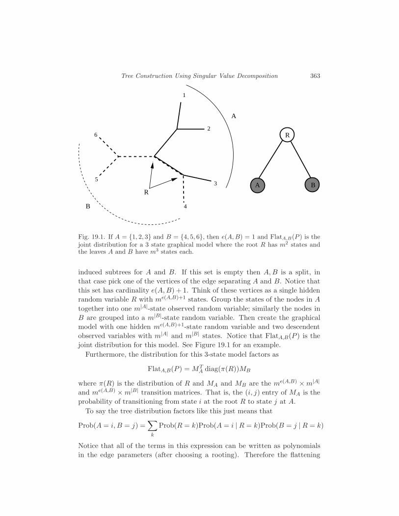
Tree Construction Using Singular Value Decomposition 363
A
R
B
1
2
4
5
6
3
A
B
R
Fig. 19.1. If A = 1, 2, 3 and B = 4, 5, 6, then e(A,B) = 1 and FlatA,B(P ) is thejoint distribution for a 3 state graphical model where the root R has m2 states andthe leaves A and B have m3 states each.
induced subtrees for A and B. If this set is empty then A,B is a split, in
that case pick one of the vertices of the edge separating A and B. Notice that
this set has cardinality e(A,B) + 1. Think of these vertices as a single hidden
random variable R with me(A,B)+1 states. Group the states of the nodes in A
together into one m|A|-state observed random variable; similarly the nodes in
B are grouped into a m|B|-state random variable. Then create the graphical
model with one hidden me(A,B)+1-state random variable and two descendent
observed variables with m|A| and m|B| states. Notice that FlatA,B(P ) is the
joint distribution for this model. See Figure 19.1 for an example.
Furthermore, the distribution for this 3-state model factors as
FlatA,B(P ) = MTA diag(π(R))MB
where π(R) is the distribution of R and MA and MB are the me(A,B) ×m|A|
and me(A,B) ×m|B| transition matrices. That is, the (i, j) entry of MA is the
probability of transitioning from state i at the root R to state j at A.
To say the tree distribution factors like this just means that
Prob(A = i, B = j) =∑
k
Prob(R = k)Prob(A = i | R = k)Prob(B = j | R = k)
Notice that all of the terms in this expression can be written as polynomials
in the edge parameters (after choosing a rooting). Therefore the flattening

364 N. Eriksson
factors, so the rank of FlatA,B(P ) is at most mmin(e(A,B)+1,|A|,|B|). It is not
hard to see that all matrices in this factorization generically have full rank
since the monomials that appear in them are distinct.
This theorem gives rise to a well known corollary upon noticing that if A,B
is a split, then e(A,B) = 0 (see [Allman and Rhodes, 2004a], for example).
Corollary 19.6 If A,B is a split in the tree, the generic rank of FlatA,B(P )
is m.
Example 19.7 In Example 19.2, the 16×16 matrix Flat1,3,2,4(P ) has rank
4 if the split 1, 3, 2, 4 occurs in the tree, otherwise, it has rank 16.
In fact, if m = 2, it has recently been shown by Allman and Rhodes
[Allman and Rhodes, 2004b] that the rank conditions in Corollary 19.6 gen-
erate the ideal of invariants for the general Markov model. However, they do
not suffice if m = 4, in that case a polynomial of degree 9 (see [Strassen, 1983,
Garcia et al., 2004]) lies in the ideal of invariants and [Landsberg and Manivel, 2004]
show that this polynomial is not generated by the degree 5 rank conditions.
19.3 Singular Value Decomposition
The SVD provides a method to compute the distance between a matrix and the
nearest rank k matrix. In this section, we briefly introduce the basic properties
of the SVD. See [Demmel, 1997] for a thorough treatment. Throughout, let A
be a m× n matrix with m ≤ n.
Definition 19.8 A singular value decomposition of a m × n matrix A is a
factorization A = UΣV T where U is n× n orthogonal, V is m×m orthogonal
and Σ =(Σ1 0
), where Σ1 = diag(σ1, σ2, . . . , σm), with σ1 ≥ σ2 ≥ · · · ≥ σm.
Definition 19.9 Let aij be the (i, j) entry of A. The Frobenius norm, written
||A||F , is the root-sum-of-squares norm on Rm·n. That is,
||A||F =√∑
a2ij .
The L2 norm, written ||A||2, is given by
||A||2 = max||x||=1
||Ax||||x||
Theorem 19.10 The distance from A to the nearest rank k matrix is
minRank(B)=k
||A−B||F =
√√√√m∑
i=k+1
σ2i ,
Tree Construction Using Singular Value Decomposition 365
in the Frobenius norm and
minRank(B)=k
||A− B||2 = σk+1
in the L2 norm.
One way of computing the singular values is to compute the eigenvalues
ofATA, the singular values are the square roots of these eigenvalues. Therefore,
general techniques to solve the real symmetric eigenvalue problem can be used
to compute the SVD. These various methods, both iterative and direct, are
implemented by many software packages for either sparse or general matrices.
We will discuss the computational issues with the SVD after we describe how
to use it to construct phylogenetic trees.
19.4 Tree Construction Algorithm
Now that we know how to tell how close a matrix is to being of a certain rank,
we can test if a given split comes from the underlying tree or not by using the
SVD to tell how close a flattening matrix is to being rank m. However, since
there are exponentially many possible splits, we must cleverly search through
this space. We do this by building the tree bottom up, at each step joining
cherries together, in a method reminiscent of neighbor joining (Algorithm 2.40).
It is an interesting open question whether the additional information in The-
orem 19.5 about non-splits that are almost splits can be harnessed to produce
an improved algorithm.
Algorithm 19.11 (Tree construction with SVD, joint with S. Snir)
Input: A multiple alignment of genome data from n species, from the alphabet
Σ with m states.
Output: An unrooted binary tree with n leaves labelled by the species.
Initialization: Compute joint probabilities pi1...in . That is, count occurrences
of each possible column of the alignment, ignoring columns with characters not
in Σ. Store the results in a sparse format.
Loop: For k from n down to 2.
For each of the(k2
)pairs of species compute the SVD for the split pair,
other k − 2 species. Pick the pair that is closest to rank m according to the
Frobenius norm and join this pair together in the tree. That is, consider this
pair as a single element when picking pairs at the next step.
Proposition 19.12 Algorithm 19.11 requires the computation of n2 SVD’s.
Proof At the first step, we compute an SVD(n2
)times. At each subsequent
366 N. Eriksson
step, we only need to compute those splits involving the pair that we just
joined together. Thus we compute (n − 2) + (n − 3) + · · · + 1 =(n−1
2
)total
SVD’s after the first step for(n2
)+(n−1
2
)= n2 SVD computations in total.
The flattenings are very large (size m|A| ×m|B|), yet they are typically very
sparse. If an alignment is of length L, at most L entries of the flattening and
typically many fewer are non-zero. Generally, computing all singular values of
a a × b matrix takes O(a2b + ab2) time. However, Lanczos iterative methods
allow singular values to be computed quickly individually, starting with the
largest. Furthermore, sparse matrix techniques allow us take advantage of this
structure without having to deal with matrices of exponential size.
Since we will be comparing the SVD from different sized splits, we need
to compute distances in the Frobenius norm, which does not change as the
dimensions of the matrices change (as long as the number of entries is constant).
This means that we should compute all singular values, however that is difficult
computationally. But in practice, the singular values typically decrease very
quickly, so it suffices to compute only the largest singular values to estimate
the Frobenius norm.
By exploiting the sparsity and only computing singular values until they
become sufficiently small, we find that we are able to very quickly compute
the SVD for for flattenings coming from trees of size at most 31 with binary
data (m = 2) and roughly size 15 with DNA data (m = 4). This limitation
is due to limits on the size of array indices in SVDLIBC and can probably
be exceeded. Furthermore, there are very good approximation algorithms (see
[Frieze et al., 1998]) for the SVD that could make very large problems practi-
cal.
Theorem 19.13 Algorithm 19.11 is statistically consistent. That is, as the
probability distribution converges to a distribution that comes from the general
Markov model on a binary tree T , the probability that Algorithm 19.11 outputs
T goes to 1.
Proof We must show that the algorithm picks a correct split at each step, that
is, that as the distribution approaches the true distribution, the probability
of choosing a bad split goes to zero. By Corollary 19.6, we see that a true
split will lead to a flattening that approaches a rank m matrix, while other
partitions will approach a matrix of higher rank (except for partitions where
one set contains only one element, however, these are never considered in the
algorithm). Therefore, as the distribution approaches the true one, the distance
from rank m of the split will go to zero while the distance from rank m of the
non-split will not go to zero.

Tree Construction Using Singular Value Decomposition 367
Example 19.14 We start with an alignment of DNA data of length 500 for 5
species, labeled 0, . . . , 4. For the first step, we look at all pairs of the 5 species.
The score column is the distance in the Frobenius norm from the flattening to
the nearest rank 4 matrix.
Split Score
0 1 | 2 3 4 2.7661
2 3 | 0 1 4 3.1513
3 4 | 0 1 2 5.9997
2 4 | 0 1 3 6.0359
0 4 | 1 2 3 6.8419
1 4 | 0 2 3 6.9895
1 3 | 0 2 4 8.0600
0 2 | 1 3 4 8.0673
1 2 | 0 3 4 8.1503
0 3 | 1 2 4 8.2082
picked split 0 1 | 2 3 4
tree is 2 3 4 (0,1)
After the first step, we see that the split 0, 1, 2, 3, 4 is best, so we join the
nodes 0, 1 together in the tree.
Split Score
2 3 | 0 1 4 3.1513
0 1 4 | 2 3 3.1513
3 4 | 0 1 2 5.9997
0 1 2 | 3 4 5.9997
0 1 3 | 2 4 6.0359
2 4 | 0 1 3 6.0359
picked split 0 1 4 | 2 3
tree is 4 (0,1) (2,3)
We have found another cherry in the tree, this time we join 2, 3 together.
Split Score
2 3 4 | 0 1 2.7661
0 1 4 | 2 3 3.1513
picked split 0 1 | 2 3 4
tree is ((0,1),(4,(2,3)))
Finally we find that node 4 should be joined with the 2, 3 cherry, and the
tree is complete.

368 N. Eriksson
b
b
a/2
b
a
b1b
b2b
b
a
b3b
b4b
b
a/2
b
a
b5b
b6b
b
a
b7b
b8b
Fig. 19.2. The 8-taxa tree used for simulation with (a, b) = (0.01, 0.07) and(0.02, 0.19).
19.5 Performance Analysis
19.5.1 Building Trees with Simulated Data
The idea of simulation is that we first pick a tree and simulate a model on
that tree to obtain aligned sequence data. Then we build a tree using Algo-
rithm 19.11 and other methods from that data and compare the answers to
the original tree.
We used the program seq-gen [Rambaut and Grassly, 1997] to simulate
data of various lengths for the tree in Figure 19.2 with various branch lengths.
This tree was chosen as a particularly difficult tree.
We simulated data under the general reversible model (the most general
model supported by seq-gen). Random numbers uniformly distributed be-
tween 1 and 2 were chosen on each run for the six transition parameters (see
Figure 4.6). The root frequencies were all set to 1/4.
Next, the data was collapsed to binary data (that is, A and G were identified,
similarly C and T). We used binary data instead of DNA data because of
numerical instability with the SVD using the much larger matrices from the
DNA data. It should be noted that Algorithm 19.11 performed better on
binary data than on DNA data. This may be due to the instability, however,
it may also be because the rank conditions define the entire ideal for binary
data.
We ran all tests using our Algorithm 19.11 as well as two algorithms from
the PHYLIP package (see Section 2.5): neighbor joining (i.e., Algorithm 2.40),
and a maximum likelihood algorithm (dnaml). All three algorithms took ap-

Tree Construction Using Singular Value Decomposition 369
0
10
20
30
40
50
60
70
80
90
100
0 200 400 600 800 1000 1200 1400 1600 1800 2000
Per
cent
of t
rees
rec
onst
ruct
ed
Sequence Length
a = 0.01, b = 0.07
SVDdnaml
NJ
Fig. 19.3. Percent of trees reconstructed correctly (for the 8 taxa tree with branchlengths (a, b) = (0.01, 0.07)) using our SVD algorithm and two PHYLIP packages.
proximately the same amount of time, except for dnaml, which slowed down
considerably for long sequences.
Figures 19.3 and 19.4 show the results of the simulations. Each algorithm
was run 1000 times for each tree and sequence length. While the SVD per-
formed slightly worse than the others, it showed very comparable behavior. It
should be noted that this tree is very difficult, requiring much more data than
a typical tree on 8 taxa.
19.5.2 Building Trees with Real Data
For data, we use the October 2004 freeze of the ENCODE alignments. For
detailed information on these, see Section 4.3, Chapters 21 and 22.
As in Chapter 21, we restricted our attention to 8 species: human, chimp,
galago, mouse, rat, cow, dog, and chicken. We processed each of the 44 EN-
CODE regions to obtain 3 data sets. First, for each region, all of the ungapped
columns were chosen. Second, within each region, all ungapped columns that
corresponded to refSeq annotated human genes were chosen. Third, we re-
stricted even further to only the human exons within the genes. Bins without
all 8 species and bins with less than 100 ungapped positions in the desired class
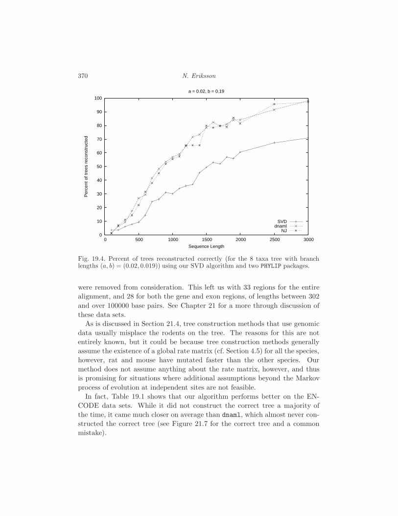
370 N. Eriksson
0
10
20
30
40
50
60
70
80
90
100
0 500 1000 1500 2000 2500 3000
Per
cent
of t
rees
rec
onst
ruct
ed
Sequence Length
a = 0.02, b = 0.19
SVDdnaml
NJ
Fig. 19.4. Percent of trees reconstructed correctly (for the 8 taxa tree with branchlengths (a, b) = (0.02, 0.019)) using our SVD algorithm and two PHYLIP packages.
were removed from consideration. This left us with 33 regions for the entire
alignment, and 28 for both the gene and exon regions, of lengths between 302
and over 100000 base pairs. See Chapter 21 for a more through discussion of
these data sets.
As is discussed in Section 21.4, tree construction methods that use genomic
data usually misplace the rodents on the tree. The reasons for this are not
entirely known, but it could be because tree construction methods generally
assume the existence of a global rate matrix (cf. Section 4.5) for all the species,
however, rat and mouse have mutated faster than the other species. Our
method does not assume anything about the rate matrix, however, and thus
is promising for situations where additional assumptions beyond the Markov
process of evolution at independent sites are not feasible.
In fact, Table 19.1 shows that our algorithm performs better on the EN-
CODE data sets. While it did not construct the correct tree a majority of
the time, it came much closer on average than dnaml, which almost never con-
structed the correct tree (see Figure 21.7 for the correct tree and a common
mistake).

Tree Construction Using Singular Value Decomposition 371
SVD dnaml
Ave. distance % correct Ave. distance % correct
All 2.06 5.8 3.29 2.9Gene 1.93 10.3 3.21 0.0Exon 2.43 21.4 3.0 3.5
Table 19.1. Comparison of the SVD algorithm and dnaml on data from the
ENCODE project. Distance between trees is given by the Robinson-Foulkes
measure.

372 N. Eriksson
s

20
Applications of Interval Methods to Phylogenetics
Raazesh Sainudiin
Ruriko Yoshida
In this chapter, we will apply interval methods to problems in phylogenetics.
An interval extension of the recursive formulation for the likelihood function
of the simplest Markov model of DNA evolution on unrooted phylogenetic
trees with a fixed topology is used to obtain rigorous enclosure(s) of the global
maximum likelihood. Thus, we can obtain the validated global maximizer(s)
inside any compact set of the parameter space which is the set of all branch
lengths of the tree. The algorithm is an adaptation of a widely applied global
optimization method using interval analysis for the phylogenetic context. The
method is applied to enclose the most likely 2, 3, and 4 taxa trees under the
simplest model of DNA evolution. The method is general and can provide
rigorous estimates when coupled with standard phylogenetic algorithms.
20.1 Interval methods for exact solutions
When statistical inference is conducted in a maximum likelihood (ML) frame-
work, one is interested in the global maximum of the likelihood function over
the parameter space. In practice one settles for a local optimization algorithm
to numerically approximate the global solution since explicit analytical solu-
tions for the maximum likelihood estimates (MLEs) are not available. How-
ever, statistical inference procedures that rely on finding some global optimum
through any numerical approach may suffer from at least five major sources of
errors. To fully appreciate the sources of errors one needs some understand-
ing of a number screen. Computers only support a finite set of numbers that
are usually represented in a semi-logarithmic manner as a set of fixed length
binary floating-point numbers of the form, x = ±m · 2e = ±0.1m2 · · ·mp · 2e,
where m is the signed mantissa (mi ∈ 0, 1, ∀i, 1 < i ≤ p) with base 2, p is
the precision, and e is the exponent (e ≤ e ≤ e) [IEEE Task P754, 1985].
Thus, the smallest and largest machine-representable numbers in absolute
value are x = 0.10 · · ·0 · 2e and x = 0.11 · · ·1 · 2e, respectively. Thus, the
373

374 R. Sainudiin and R. Yoshida
binary floating-point system of most machines R = R(2, p, e, e) is said to form
a screen of the real numbers in the interval [−x,+x] with 0 uniquely rep-
resented by 0.00 · · ·0 · 2e. Arithmetic on a machine is typically performed
with such a screen in an inexact manner and may suffer from the following
errors: roundoff error – the difference between computed and exact result
[Cuyt et al., 2001, Loh and Walster, 2002], truncation error – from having to
truncate an infinite sequence of operations, conversion error – inability to
machine-represent decimals with infinite binary expansion, and ill-posed sta-
tistical experiment – presence of unknown nonidentifiable subspaces.
The verified global optimization method [Hansen, 1980] sketched below rig-
orously encloses the global maximum of the likelihood function through interval
analysis [Moore, 1967]. Such interval methods evaluate the likelihood function
over a continuum of points including those that are not machine-representable
and account for all sources of errors described earlier. In the sequel we will see
that interval methods, in contrast to heuristic local search methods, can enclose
the global optimum with guaranteed accuracy by exhaustive search within any
compact set of the parameter space. We begin with a brief introduction to
interval analysis.
Lower case letters denote real numbers, e.g. x ∈ R. Upper case letters
represent compact real intervals, e.g. X = [x, x] = [inf(X), sup(X)]. Any
compact interval X ∈ IR := [a, b] : a ≤ b, a, b ∈ R, the set of all compact
real intervals. The diameter and the midpoint of X are d(X) := x − x and
m(X) := (x + x)/2, respectively. The magnitude of X is 〈X〉 := min|x| :
x ∈ X = min|x|, |x|, if 0 /∈ X , and 0 otherwise. The magnitude of X
is |X | := max|x| : x ∈ X = max|x|, |x|, while the absolute value of an
interval X is |X |[ ] := |x| : x ∈ X = [〈X〉, |X |]. The relative diameter of an
interval X , denoted by drel, is the diameter d(X) itself if 0 ∈ X and d(X)/〈X〉otherwise. An interval X with zero diameter is called a thin interval with
x = x = x. The hull of two intervals is X∪Y := [minx, y,minx, y].By the notation X ⋐ Y , it is meant that X is completely contained in Y ,
i.e. x > y and x < y. No notational distinction is made between a real
number x ∈ R and a real vector x = (xi, · · · , xn)T ∈ Rn and between a
real interval X and a real interval vector or box X = (X1, · · · , Xn)T ∈ IRn,
i.e. Xi = [xi, xi] = [inf(Xi), sup(Xi)] ∈ IR, where i = 1, · · · , n. For an inter-
val vector X , the diameter, relative diameter, midpoint, and hull operations
are defined component-wise to yield vectors, while the maximum over its com-
ponents is taken to obtain the maximal diameter and the maximal relative
diameter, d∞(X) = maxi d(Xi) and drel,∞(X) = maxi drel(Xi), respectively.
Also IR under the metric h, given by h(X, Y ) := max|x−y|, |x−y|, is a com-
plete metric space. Convergence of a sequence of intervals X (i) to an interval
X under the metric h is equivalent to the sequence h(X (i), X) approaching 0
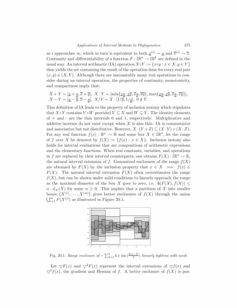
Applications of Interval Methods to Phylogenetics 375
as i approaches ∞, which in turn is equivalent to both x(i) → x and x(i) → x.
Continuity and differentiability of a function F : IRn → IRk are defined in the
usual way. An interval arithmetic (IA) operationXY := xy : x ∈ X, y ∈ Y thus yields the set containing the result of the operation done for every real pair
(x, y) ∈ (X, Y ). Although there are uncountably many real operations to con-
sider during an interval operation, the properties of continuity, monotonicity,
and compactness imply that:
X + Y = [x+ y, x+ y], X · Y = [minxy, xy, xy, xy,maxxy, xy, xy, xy],X − Y = [x− y, x− y], X/Y = X · [1/y, 1/y], 0 /∈ Y.
This definition of IA leads to the property of inclusion isotony which stipulates
that X Y contains V W provided V ⊆ X and W ⊆ Y . The identity elements
of + and · are the thin intervals 0 and 1, respectively. Multiplicative and
additive inverses do not exist except when X is also thin. IA is commutative
and associative but not distributive. However, X · (Y +Z) ⊆ (X ·Y )+ (X ·Z).
For any real function f(x) : Rn → R and some box X ∈ IRn, let the range
of f over X be denoted by f(X) := f(x) : x ∈ X. Inclusion isotony also
holds for interval evaluations that are compositions of arithmetic expressions
and the elementary functions. When real constants, variables, and operations
in f are replaced by their interval counterparts, one obtains F (X) : IRn → R,
the natural interval extension of f . Guaranteed enclosures of the range f(X)
are obtained by F (X) by the inclusion property that x ∈ X =⇒ f(x) ∈F (X). The natural interval extension F (X) often overestimates the range
f(X), but can be shown under mild conditions to linearly approach the range
as the maximal diameter of the box X goes to zero, i.e. h(F (X), f(X)) ≤α · d∞(X) for some α ≥ 0. This implies that a partition of X into smaller
boxes X (1), · · · , X (m) gives better enclosures of f(X) through the union⋃mi=1 F (X (i)) as illustrated in Figure 20.1.
-10 -7.5 -5 -2.5 0 2.5 5
-150
-100
-50
0
50
100
150
Fig. 20.1. Range enclosure of −∑5k=1 k x sin (k(x−3)
3 ) linearly tightens with mesh
Let F (x) and 2F (x) represent the interval extensions of f(x) and
2f(x), the gradient and Hessian of f . A better enclosure of f(X) is pos-
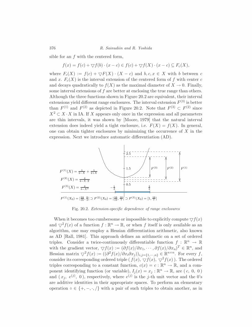
376 R. Sainudiin and R. Yoshida
sible for an f with the centered form,
f(x) = f(c) + f(b) · (x− c) ∈ f(c) + f(X) · (x− c) ⊆ Fc(X),
where Fc(X) := f(c) + F (X) · (X − c) and b, c, x ∈ X with b between c
and x. Fc(X) is the interval extension of the centered form of f with center c
and decays quadratically to f(X) as the maximal diameter of X → 0. Finally,
some interval extensions of f are better at enclosing the true range than others.
Although the three functions shown in Figure 20.2 are equivalent, their interval
extensions yield different range enclosures. The interval extension F (3) is better
than F (1) and F (2) as depicted in Figure 20.2. Note that F (3) ⊂ F (2) since
X2 ⊂ X ·X in IA. If X appears only once in the expression and all parameters
are thin intervals, it was shown by [Moore, 1979] that the natural interval
extension does indeed yield a tight enclosure, i.e. F (X) = f(X). In general,
one can obtain tighter enclosures by minimizing the occurrence of X in the
expression. Next we introduce automatic differentiation (AD).
F (1)
0.5
1.5
2.5
F (2)
F(1)(X) = 1
2−X + 12+X
F(2)(X) = 4
4−X·X
F(3)(X) = 4
4−X2
F (1)(X0) = [ 2435
, 83] ⊃ F (2)(X0) = [ 16
19, 16
7] ⊃ F (3)(X0) = [1, 16
7]
− 12
32
F (3)
Fig. 20.2. Extension-specific dependence of range enclosures
When it becomes too cumbersome or impossible to explicitly compute f(x)
and 2f(x) of a function f : Rn → R, or when f itself is only available as an
algorithm, one may employ a Hessian differentiation arithmetic, also known
as AD [Rall, 1981]. This approach defines an arithmetic on a set of ordered
triples. Consider a twice-continuously differentiable function f : Rn → Rwith the gradient vector, f(x) := (∂f(x)/∂x1, · · · , ∂f(x)/∂xn)
T ∈ Rn, and
Hessian matrix 2f(x) := ((∂2f(x)/∂xi∂xj))i,j=1,··· ,n ∈ Rn×n. For every f ,
consider its corresponding ordered triple ( f(x), f(x), 2f(x) ). The ordered
triples corresponding to a constant function, c(x) = c : Rn → R, and a com-
ponent identifying function (or variable), Ij(x) = xj : Rn → R, are ( c, 0, 0 )
and ( xj, e(j), 0 ), respectively, where e(j) is the j-th unit vector and the 0’s
are additive identities in their appropriate spaces. To perform an elementary
operation ∈ +,−, ·, / with a pair of such triples to obtain another, as in
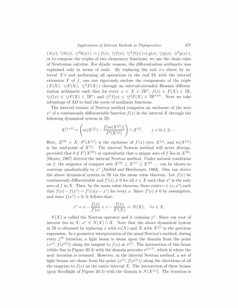
Applications of Interval Methods to Phylogenetics 377
( h(x), h(x), 2h(x) ) := ( f(x), f(x), 2f(x) )( g(x), g(x), 2g(x) ),
or to compose the triples of two elementary functions, we use the chain rules
of Newtonian calculus. For dyadic reasons, the differentiation arithmetic was
explained only in terms of reals. By replacing the real x’s above by in-
terval X ’s and performing all operations in the real IA with the interval
extension F of f , one can rigorously enclose the components of the triple
(F (X), F (X), 2F (X) ) through an interval-extended Hessian differen-
tiation arithmetic such that for every x ∈ X ∈ IRn, f(x) ∈ F (X) ∈ IR,
f(x) ∈ F (X) ∈ IRn, and 2f(x) ∈ 2F (X) ∈ IRn×n. Next we take
advantage of AD to find the roots of nonlinear functions.
The interval version of Newton method computes an enclosure of the zero
x∗ of a continuously differentiable function f(x) in the interval X through the
following dynamical system in IR:
X (j+1) =
(m(X (j)) − f(m(X (j)))
F ′(X (j))
)∩X (j), j = 0, 1, 2, · · ·
Here, X (0) = X , F ′(X (j)) is the enclosure of f ′(x) over X (j), and m(X (j))
is the mid-point of X (j). The interval Newton method will never diverge,
provided that 0 /∈ F ′(X (0)) or equivalently that a unique zero of f lies in X (0).
[Moore, 1967] derived the interval Newton method. Under natural conditions
on f , the sequence of compact sets X (0) ⊇ X (1) ⊇ X (2) · · · can be shown to
converge quadratically to x∗ [Alefeld and Herzberger, 1983]. One can derive
the above dynamical system in IR via the mean value theorem. Let f(x) be
continuously differentiable and f ′(x) 6= 0 for all x ∈ X such that x∗ is the only
zero of f in X . Then, by the mean value theorem, there exists c ∈ (x, x∗) such
that f(x)− f(x∗) = f ′(c)(x− x∗) for every x. Since f ′(c) 6= 0 by assumption,
and since f(x∗) = 0, it follows that:
x∗ = x− f(x)
f ′(c)∈ x− f(x)
F ′(X)=: N (X), ∀x ∈ X.
N (X) is called the Newton operator and it contains x∗. Since our root of
interest lies in X , x∗ ∈ N (X) ∩ X . Note that the above dynamical system
in IR is obtained by replacing x with m(X) and X with X (j) in the previous
expression. In a geometric interpretation of the usual Newton’s method, during
every jth iteration, a light beam is shone upon the domain from the point
(x(j), f(x(j))) along the tangent to f(x) at x(j). The intersection of this beam
(white line in Figure 20.3) with the domain provides x(j+1), which is where the
next iteration is resumed. However, in the interval Newton method, a set of
light beams are shone from the point (x(j), f(x(j))) along the directions of all
the tangents to f(x) on the entire interval X . The intersection of these beams
(gray floodlight of Figure 20.3) with the domain is N (X (j)). The iteration is
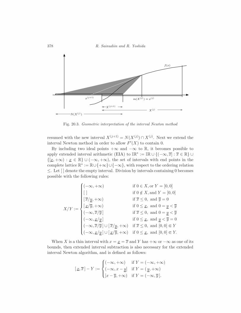
378 R. Sainudiin and R. Yoshida
f(x)
m(X(j)) = x(j)
X(j)
x(j+1)
N(X(j))
X(j+1)
Fig. 20.3. Geometric interpretation of the interval Newton method
resumed with the new interval X (j+1) = N (X (j)) ∩X (j). Next we extend the
interval Newton method in order to allow F ′(X) to contain 0.
By including two ideal points +∞ and −∞ to R, it becomes possible to
apply extended interval arithmetic (EIA) to IR∗ := IR ∪ (−∞, x] : x ∈ R ∪[x,+∞) : x ∈ R ∪ (−∞,+∞), the set of intervals with end points in the
complete lattice R∗ := R∪+∞∪−∞, with respect to the ordering relation
≤. Let [ ] denote the empty interval. Division by intervals containing 0 becomes
possible with the following rules:
X/Y :=
(−∞,+∞) if 0 ∈ X, or Y = [0, 0]
[ ] if 0 /∈ X, and Y = [0, 0]
[ x/y,+∞) if x ≤ 0, and y = 0
[ x/y,+∞) if 0 ≤ x, and 0 = y < y
(−∞, x/y ] if x ≤ 0, and 0 = y < y
(−∞, x/y ] if 0 ≤ x, and y < y = 0
(−∞, x/y ] ∪ [ x/y,+∞) if x ≤ 0, and [0, 0] ⋐ Y
(−∞, x/y ] ∪ [ x/y,+∞) if 0 ≤ x, and [0, 0] ⋐ Y.
When X is a thin interval with x = x = x and Y has +∞ or −∞ as one of its
bounds, then extended interval subtraction is also necessary for the extended
interval Newton algorithm, and is defined as follows:
[ x, x ]− Y :=
(−∞,+∞) if Y = (−∞,+∞)
(−∞, x− y] if Y = ( y,+∞)
[x− y,+∞) if Y = (−∞, y ].
Applications of Interval Methods to Phylogenetics 379
The extended interval Newton method uses the EIA described above and
is a variant of the method based on [Hansen and Sengupta, 1981] with Ratz’s
modifications [Ratz, 1992] as implemented in [Hammer et al., 1995]. It can be
used to enclose the roots of a continuously differentiable f : Rn → Rn in a
given box X ∈ IRn. Let Jf (x) := ((∂fi(x)/∂xj))i,j=1,··· ,n ∈ Rn×n denote
the Jacobian matrix of f at x. Let JF (X) ⊃ Jf(X) denote the Jacobian
of the interval extension of f . The Jacobian can be computed via AD by
computing the gradient of each component fi of f . By the mean value theorem,
f(m(X))−f(x∗) = Jf (w)·(m(X)−x∗), for some x∗ ∈ X,w = (w1, w2, · · · , wn),
where wi ∈ X, ∀i ∈ 1, 2, · · · , n. Interest in x∗ with f(x∗) = 0 yields the
following relation provided that JF (x) ∀x ∈ X is invertible: x∗ ∈ N (X) ∩ X ,
where N (X) := m(X)−( JF (X) )−1 ·F (m(X)). An iteration scheme X (j+1) :=
N (X (j)) ∩ X (j) for j = 0, 1, · · · , and X (0) := X will enclose the zeros of
f contained in X . To relax the assumption that every matrix in JF (X) be
invertible, the inverse of the midpoint of JF (X), i.e. (m(JF (X)))−1 =: p ∈Rn×n, is used as a matrix preconditioner. The extended interval Gauss-Seidel
iteration, which is also applicable to singular systems [Neumaier, 1990], is used
to solve the preconditioned interval linear equation,
p · F (m(X)) = p · JF (X) · (m(X)− x∗)
a = G · (c− x∗),
where a ∈ A := p · F (m(X)), G := p · JF (X), and c := m(X). Thus, the
solution set S := x ∈ X : g · (c − x) = a, ∀g ∈ G of the interval linear
equation a = G · (c− x) has the component-wise solution set Si = xi ∈ Xi :∑nj=1 ( gi,j · (cj − xj) ) = ai, ∀g ∈ G, ∀i ∈ 1, · · · , n. Now set Y = X , and
solve the ith equation for the ith variable iteratively for each i as follows:
yi = ci − 1gi,i
(ai +
∑nj=1,j 6=i( gi,j · (yj − cj) )
)
∈(ci − 1
Gi,i
(Ai +
∑nj=1,j 6=i(Gi,j · (Yj − cj) )
))∩ Yi.
The interval vector(s) Y obtained at the end of such an iteration is the set,
NGS(X), resulting from one extended interval Newton Gauss-Seidel step such
that S ⊆ NGS(X) ⊆ X . Thus, the roots of f are enclosed by the discrete
dynamical system X (j) = NGS(X (j)) in IRn. Every 0 of f that lies in X also
lies in NGS(X). If NGS(X) = [ ], the empty interval, then f has no solution
in X . If NGS (X) ⋐ X , then f has a unique solution in X [Hansen, 1992].
When Gii ⊃ 0, the method is applicable with EIA that allows for division by
0. In such cases, one may obtain up to two disjoint compact intervals for Yi
subsequent to EIA and intersection with the previous compact interval Xi. In
such cases, the iteration is applied to each resulting sub-interval.
All IA was done above with real intervals. However, R, the set of floating-
380 R. Sainudiin and R. Yoshida
point numbers available on a computing machine, is finite. A machine interval
is a real interval with floating-point bounds. One works with IR := X ∈IR : x, x ∈ R, the set of all machine intervals, in a computer. In spite of the
finiteness of IR, the strength of IA lies in a machine interval X being able to
enclose the entire continuum of reals between its machine-representable bound-
aries. Operations with real intervals can be tightly enclosed by the rounding di-
rected operations, provided by the IEEE arithmetic standard, with the smallest
machine intervals containing them [Hammer et al., 1995, Kulisch et al., 2001].
20.2 Enclosing the likelihood of a compact set of trees
Let D denote a homologous set of distinct DNA sequences of length v from n
species. We want the MLEs of branch lengths for the most likely tree under
a particular topology. Let b denote the number of branches and s denote the
number of nodes of a tree with topology τ . Thus, for a given unrooted topology
τ with n leaves and b branches, the unknown parameter θ = ( θ1, · · · , θb ) is
the real vector of branch lengths in the positive orthant (θq ∈ R+). An explicit
model of DNA evolution is needed to construct the likelihood function which
gives the probability of observing data D as a function of the parameter θ.
The simplest such continuous time Markov chain model (JC69) on the state
space Σ is due to [Jukes and Cantor, 1969]. One may compute ℓ(k)(θ), the
log likelihood at site k ∈ 1, · · · , v through the following post-order traversal
[Felsenstein, 1981]:
(i) Associate with each node q ∈ 1, · · · , s with m descendants, a partial
likelihood vector, lq := (lAq , lCq , l
Gq , l
Tq ) ∈ R4, and let the length of the
branch leading to its ancestor be θq.
(ii) For a leaf node q with nucleotide i, set liq = 1 and ljq = 0 for all j 6= i.
For any internal node q, set lq := (1, 1, 1, 1).
(iii) For an internal node q with descendants s1, s2, · · · , sm,
liq =∑
j1,··· ,jm∈Σ
lj1s1· Pi,j1(θs1) · lj2s2
· Pi,j2(θs2) · · · ljmsm
· Pi,jm(θsm) .
(iv) Compute lq for each sub-terminal node q, then those of their ancestors
recursively to finally compute lr for the root node r to obtain the log
likelihood for site k, ℓ(k)(θ) = lr = log∑
i∈Σ (πi · lir ).
Assuming independence across sites one obtains ℓ(θ) =∑v
k=1 ℓ(k)(θ), the nat-
ural logarithm of the likelihood function for the data D by multiplying the
site-specific likelihoods. The problem of finding the global maximum of this
likelihood function is equivalent to finding the global minimum of l(θ) := −ℓ(θ).Replacing every constant c by its corresponding constant triple (C, 0, 0), every

Applications of Interval Methods to Phylogenetics 381
variable θj by its triple ( Θj, e(j), 0 ), and every real operation or elementary
function by its counterpart in interval-extended Hessian differentiation arith-
metic in the above post-order traversal yields a rigorous enclosure of the nega-
tive log likelihood triple (L(Θ),L(Θ),2L(Θ) ) of the negative log likelihood
function l(θ) over Θ.
20.3 Global Optimization
20.3.1 Branch-and-bound
The most basic strategy in global optimization through enclosure methods is
to employ rigorous branch-and-bound techniques. Such techniques recursively
partition (branch) the original compact space of interest into compact sub-
spaces and discard (bound) those subspaces that are guaranteed to not contain
the global optimizer(s). For the real scalar-valued multi-dimensional objective
function l(θ), the interval branch-and-bound technique can be applied to its
natural interval extension L(Θ) to obtain an interval enclosure L∗ of the global
minimum value l∗ as well as the set of minimizer(s) to a specified accuracy ǫ.
Note that this set of minimizer(s) of L(θ) is the set of maximizer(s) of the
likelihood function for the observed data D. The strength of such methods
arises from the algorithmic ability to discard large sub-boxes from the original
search region,
Θ(0) = ( Θ(0)1 , · · · ,Θ(0)
b ) := ( [θ(0)1 , θ
(0)1 ], · · · , [θ (0)
b , θ(0)b ] ) ⊂ IRb,
that are not candidates for global minimizer(s). Four tests that help discard
sub-regions are described below. Let L denote a list of ordered pairs of the
form ( Θ(i),LΘ(i) ), where Θ(i) ⊆ Θ(0), and LΘ(i) := min (L(Θ(i)) ) is a lower
bound for the range of the negative log likelihood function l over Θ(i). Let l be
an upper bound for l∗ and L(Θ(i))k denote the k-th interval of the gradient
box L(Θ(i)). If no information is available for l, then l = ∞.
20.3.1.1 Midpoint cut-off test
The basic idea of the midpoint cut-off test is to discard sub-boxes of the search
space Θ(0) with the lower bound for their range enclosures above l, the current
best estimate of an upper bound for l∗. Figure 20.4 shows a multi-modal l as a
function of a scalar valued θ over Θ(0) = ∪16i=1Θ
(i). For this illustrative example,
l is set as the upper bound of the range enclosure of l over the smallest machine
interval containing the midpoint of Θ(15), the interval with the smallest lower
bound of its range enclosure. The shaded rectangles show the range enclosures
over intervals that lie strictly above l. In this example the midpoint cut-off test
would discard all other intervals except Θ(1), Θ(2), and Θ(4).
• Given a list L and l.
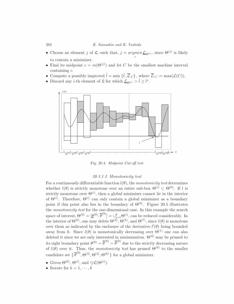
382 R. Sainudiin and R. Yoshida
• Choose an element j of L, such that, j = argmini
LΘ(i) , since Θ(j) is likely
to contain a minimizer.
• Find its midpoint c = m(Θ(j)) and let C be the smallest machine interval
containing c.
• Compute a possibly improved l = min l ,L C , where L C := max(L(C)).
• Discard any i-th element of L for which LΘ(i) > l ≥ l∗.
Θ(16)
l(θ)
θ
l
Θ(4)Θ(3)Θ(2)Θ(1) Θ(15)
Fig. 20.4. Midpoint Cut-off test
20.3.1.2 Monotonicity test
For a continuously differentiable function l(θ), the monotonicity test determines
whether l(θ) is strictly monotone over an entire sub-box Θ(i) ⊂ Θ(0). If l is
strictly monotone over Θ(i), then a global minimizer cannot lie in the interior
of Θ(i). Therefore, Θ(i) can only contain a global minimizer as a boundary
point if this point also lies in the boundary of Θ(0). Figure 20.5 illustrates
the monotonicity test for the one-dimensional case. In this example the search
space of interest, Θ(0) = [θ(0), θ(0)
] = ∪8i=1Θ
(i), can be reduced considerably. In
the interior of Θ(0), one may delete Θ(2), Θ(5), and Θ(7), since l(θ) is monotone
over them as indicated by the enclosure of the derivative l′(θ) being bounded
away from 0. Since l(θ) is monotonically decreasing over Θ(1) one can also
deleted it since we are only interested in minimization. Θ(8) may be pruned to
its right boundary point θ(8) = θ(8)
= θ(0)
due to the strictly decreasing nature
of l(θ) over it. Thus, the monotonicity test has pruned Θ(0) to the smaller
candidate set θ(0),Θ(3),Θ(4),Θ(6) for a global minimizer.
• Given Θ(0), Θ(i), and L(Θ(i)).
• Iterate for k = 1, · · · , b
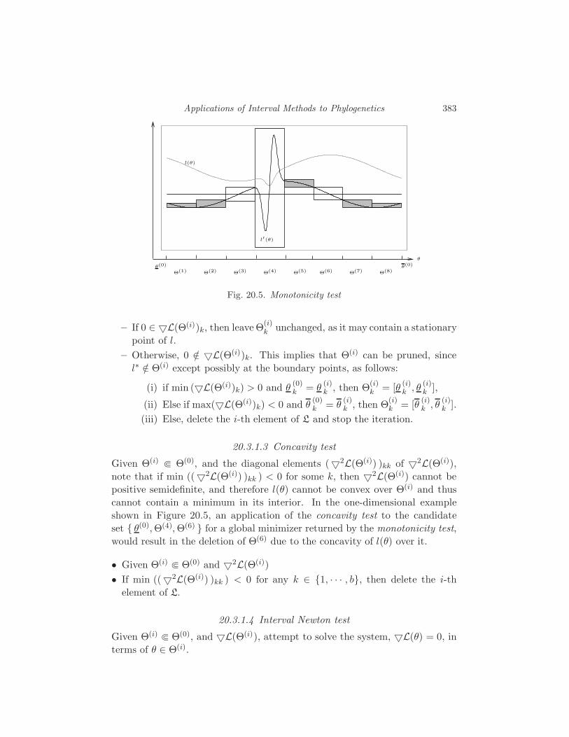
Applications of Interval Methods to Phylogenetics 383
θ
θ(0)θ(0)
Θ(7) Θ(8)Θ(1) Θ(2) Θ(3) Θ(4) Θ(5) Θ(6)
l(θ)
l′(θ)
Fig. 20.5. Monotonicity test
– If 0 ∈ L(Θ(i))k, then leave Θ(i)k unchanged, as it may contain a stationary
point of l.
– Otherwise, 0 /∈ L(Θ(i))k. This implies that Θ(i) can be pruned, since
l∗ /∈ Θ(i) except possibly at the boundary points, as follows:
(i) if min (L(Θ(i))k) > 0 and θ(0)k = θ
(i)k , then Θ
(i)k = [θ
(i)k , θ
(i)k ],
(ii) Else if max(L(Θ(i))k) < 0 and θ(0)k = θ
(i)k , then Θ
(i)k = [θ
(i)k , θ
(i)k ].
(iii) Else, delete the i-th element of L and stop the iteration.
20.3.1.3 Concavity test
Given Θ(i)⋐ Θ(0), and the diagonal elements (2L(Θ(i)) )kk of 2L(Θ(i)),
note that if min ((2L(Θ(i)) )kk ) < 0 for some k, then 2L(Θ(i)) cannot be
positive semidefinite, and therefore l(θ) cannot be convex over Θ(i) and thus
cannot contain a minimum in its interior. In the one-dimensional example
shown in Figure 20.5, an application of the concavity test to the candidate
set θ(0),Θ(4),Θ(6) for a global minimizer returned by the monotonicity test,
would result in the deletion of Θ(6) due to the concavity of l(θ) over it.
• Given Θ(i)⋐ Θ(0) and 2L(Θ(i))
• If min ((2L(Θ(i)) )kk ) < 0 for any k ∈ 1, · · · , b, then delete the i-th
element of L.
20.3.1.4 Interval Newton test
Given Θ(i)⋐ Θ(0), and L(Θ(i)), attempt to solve the system, L(θ) = 0, in
terms of θ ∈ Θ(i).

384 R. Sainudiin and R. Yoshida
• Apply one extended interval Newton Gauss-Seidel step to the linear interval
equation a = G · (c − θ), where a := p · L(m(Θ(i))), G := p · 2L(Θ(i)),
c := m(Θ(i)), and p := (m(2F (X)))−1, in order to obtain N ′GS(Θ(i)).
• One of the following can happen,
(i) If N ′GS(Θ(i)) is empty, then discard Θ(i).
(ii) If N ′GS(Θ(i)) ⋐ Θ(i), then replace Θ(i) by the contraction N ′GS (Θ(i))∩Θ(i).
(iii) If 0 ∈ Gjj , and the extended interval division splits Θ(i)j into a non-
empty union of Θ(i),1j and Θ
(i),2j , then the iteration is continued on
Θ(i),1j , while Θ
(i),2j , if non-empty, is stored in L for future processing.
Thus, one extended interval Newton Gauss-Seidel step can add at
most b+ 1 sub-boxes to L.
20.3.2 Verification
Given a collection of sub-boxes, Θ(1), · · · ,Θ(n) , each of width ≤ ǫ, that
could not be discarded by the tests in Section 20.3.1, one can attempt to verify
the existence and uniqueness of a local minimizer within each sub-box θ(i) by
checking whether the conditions of the following two theorems are satisfied.
For proof of these two theorems see [Hansen, 1992] and [Ratz, 1992].
(i) If N ′GS(Θ(i)) ⋐ Θ(i), then there exists a unique stationary point of L,
i.e. a unique zero of L exists in Θ(i).
(ii) If ( I + 1κ · (2L(Θ(i))) ) · Z ⋐ Z, where (2L(Θ(i)))d,∞ ≤ κ ∈ R, for
some Z ∈ IRn, then the spectral radius ρ(s) < 1 for all s ∈ ( I −1κ · (2L(Θ(i))) ) and all symmetric matrices in 2L(Θ(i)) are positive
definite.
If the conditions of the above two theorems are satisfied by some Θ(i), then a
unique stationary point exists in Θ(i) and this stationary point is a local min-
imizer. Therefore, if exactly one candidate sub-box for minimizer(s) remained
after pruning the search box Θ(0) with the tests in Section 20.3.1, and if this
sub-box satisfies the above two conditions for the existence of a unique local
minimizer within it, then one has rigorously enclosed the global minimizer in
the search interval. On the other hand, if there are two or more sub-boxes
in our candidate list for minimizer(s) that satisfy the above two conditions,
then one may conclude that each sub-box contains a candidate for a global
minimizer which may not necessarily be unique (disconnected sub-boxes, for
example). Observe that failure to verify the uniqueness of a local minimizer in
a sub-box can occur if it contains two or more points or even a continuum of
points that are stationary.
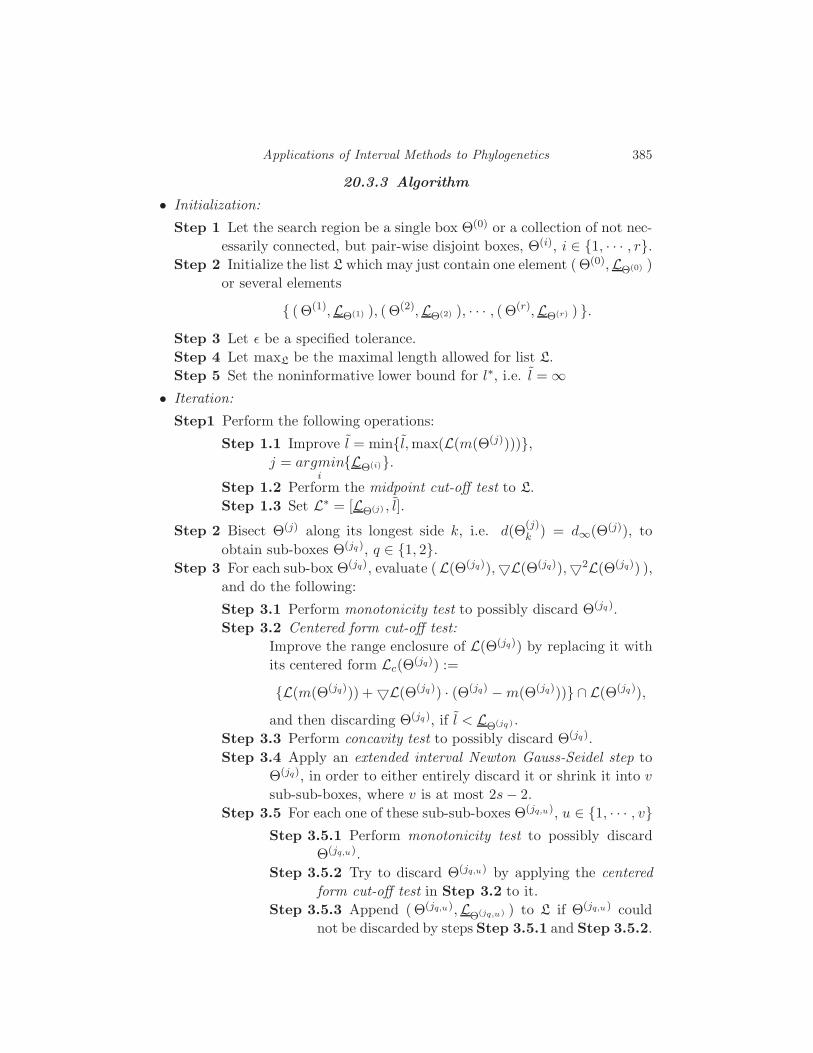
Applications of Interval Methods to Phylogenetics 385
20.3.3 Algorithm
• Initialization:
Step 1 Let the search region be a single box Θ(0) or a collection of not nec-
essarily connected, but pair-wise disjoint boxes, Θ(i), i ∈ 1, · · · , r.Step 2 Initialize the list L which may just contain one element ( Θ(0),LΘ(0) )
or several elements
( Θ(1),LΘ(1) ), ( Θ(2),LΘ(2) ), · · · , ( Θ(r),LΘ(r) ) .Step 3 Let ǫ be a specified tolerance.
Step 4 Let maxL be the maximal length allowed for list L.
Step 5 Set the noninformative lower bound for l∗, i.e. l = ∞• Iteration:
Step1 Perform the following operations:
Step 1.1 Improve l = minl,max(L(m(Θ(j)))),j = argmin
iLΘ(i).
Step 1.2 Perform the midpoint cut-off test to L.
Step 1.3 Set L∗ = [LΘ(j) , l].
Step 2 Bisect Θ(j) along its longest side k, i.e. d(Θ(j)k ) = d∞(Θ(j)), to
obtain sub-boxes Θ(jq), q ∈ 1, 2.Step 3 For each sub-box Θ(jq), evaluate (L(Θ(jq)),L(Θ(jq)),2L(Θ(jq)) ),
and do the following:
Step 3.1 Perform monotonicity test to possibly discard Θ(jq).
Step 3.2 Centered form cut-off test:
Improve the range enclosure of L(Θ(jq)) by replacing it with
its centered form Lc(Θ(jq)) :=
L(m(Θ(jq))) + L(Θ(jq)) · (Θ(jq) −m(Θ(jq))) ∩ L(Θ(jq)),
and then discarding Θ(jq), if l < LΘ(jq ) .
Step 3.3 Perform concavity test to possibly discard Θ(jq).
Step 3.4 Apply an extended interval Newton Gauss-Seidel step to
Θ(jq), in order to either entirely discard it or shrink it into v
sub-sub-boxes, where v is at most 2s− 2.
Step 3.5 For each one of these sub-sub-boxes Θ(jq,u), u ∈ 1, · · · , vStep 3.5.1 Perform monotonicity test to possibly discard
Θ(jq,u).
Step 3.5.2 Try to discard Θ(jq,u) by applying the centered
form cut-off test in Step 3.2 to it.
Step 3.5.3 Append ( Θ(jq,u),LΘ(jq,u) ) to L if Θ(jq,u) could
not be discarded by steps Step 3.5.1 and Step 3.5.2.
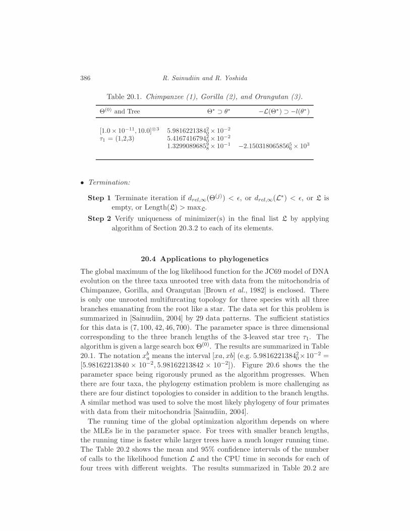
386 R. Sainudiin and R. Yoshida
Table 20.1. Chimpanzee (1), Gorilla (2), and Orangutan (3).
Θ(0) and Tree Θ∗ ⊃ θ∗ −L(Θ∗) ⊃ −l(θ∗)
[1.0× 10⁻¹¹, 10.0]⊗3 5.981622138420 × 10⁻²
τ1 = (1,2,3) 5.416741679420 × 10⁻²
1.329908968598 × 10⁻¹ −2.1503180658565
6 × 10³
• Termination:
Step 1 Terminate iteration if drel,∞(Θ(j)) < ǫ, or drel,∞(L∗) < ǫ, or L is
empty, or Length(L) > maxL.
Step 2 Verify uniqueness of minimizer(s) in the final list L by applying
algorithm of Section 20.3.2 to each of its elements.
20.4 Applications to phylogenetics
The global maximum of the log likelihood function for the JC69 model of DNA
evolution on the three taxa unrooted tree with data from the mitochondria of
Chimpanzee, Gorilla, and Orangutan [Brown et al., 1982] is enclosed. There
is only one unrooted multifurcating topology for three species with all three
branches emanating from the root like a star. The data set for this problem is
summarized in [Sainudiin, 2004] by 29 data patterns. The sufficient statistics
for this data is (7, 100, 42, 46, 700). The parameter space is three dimensional
corresponding to the three branch lengths of the 3-leaved star tree τ1. The
algorithm is given a large search box Θ(0). The results are summarized in Table
20.1. The notation xba means the interval [xa, xb] (e.g. 5.98162213842
0×10−2 =
[5.98162213840 × 10⁻², 5.98162213842 × 10⁻²]). Figure 20.6 shows the the
parameter space being rigorously pruned as the algorithm progresses. When
there are four taxa, the phylogeny estimation problem is more challenging as
there are four distinct topologies to consider in addition to the branch lengths.
A similar method was used to solve the most likely phylogeny of four primates
with data from their mitochondria [Sainudiin, 2004].
The running time of the global optimization algorithm depends on where
the MLEs lie in the parameter space. For trees with smaller branch lengths,
the running time is faster while larger trees have a much longer running time.
The Table 20.2 shows the mean and 95% confidence intervals of the number
of calls to the likelihood function L and the CPU time in seconds for each of
four trees with different weights. The results summarized in Table 20.2 are

Applications of Interval Methods to Phylogenetics 387
0
5
0
5
5
0
5
0
5
0
0.25
0
0.25
0.25
0
0.25
0
0.25
0.059
0.0605
0.0535
0.055
0.132
0.133
0.059
0.0605
0.0535
0.055
0.059
0.0605
0.0535
0.055
0.132
0.133
0.059
0.0605
0.0535
0.055
05
10
0
5
10
5
10
05
10
0
5
10
05
10
0
5
10
5
10
05
10
0
5
10
05
10
0
5
10
5
10
05
10
0
5
10
0
5
0
5
5
0
5
0
5
Fig. 20.6. Progress of the algorithm as it prunes [0.001, 10.0]⊗3.
Table 20.2. Computational efficiency for four different 3 taxa trees.
True Tree Calls to L(Θ∗) CPU time
(1 : 0.01, 2 : 0.07, 3 : 0.07) 1272 [1032, 1663] 0.55 [0.45, 0.72](1 : 0.02, 2 : 0.19, 3 : 0.19) 3948 [2667, 6886] 1.75 [1.17, 3.05](1 : 0.03, 2 : 0.42, 3 : 0.42) 20789 [12749, 35220] 9.68 [5.94, 16.34](1 : 0.06, 2 : 0.84, 3 : 0.84) 245464 [111901, 376450] 144.62 [64.07, 232.94]
from 100 data sets, each of sequence length 1000, simulated under JC69 model
upon each one of the four trees shown in the first column.
The MLEs obtained by means of interval methods are equivalent to numer-
ical proofs for the MLEs. The method is robust in the presence of multiple
local maxima or nonidentifiable manifolds with the same ML value. For ex-
ample, when a time reversible Markov chain, such as JC69, is super-imposed
on a rooted tree, only the sum of the branch lengths emanating from the
root is identifiable. Identifiability is a prerequisite for statistical consistency
of estimators. To demonstrate the ability of interval methods to enclose the
nonidentifiable ridge along θ1 + θ2 in the simplest case of a two-leaved tree, a
nonidentifiable negative log likelihood function l(θ1, θ2) is formulated with its
global minimizers along θ1 + θ2 = 34 log (45/17) = 0.730087 under a fictitious
dataset for which 280 out of 600 sites are polymorphic. Figure 20.7 shows the
contours of l(θ1, θ2) in gray scale and the solutions of the interval method (gray
and black rectangles) and those of 10 Quasi-Newton searches with random ini-
tializations (10 pairs of colored ovals). Observe that the basin of attraction for
each point on θ1 +θ2 = 0.730087 under a Quasi-Newton local search algorithm
is the line running orthogonal to it.
Interval methods can be slow on currently available processors that are op-
timized for floating-point arithmetic, especially when applied naively. If one
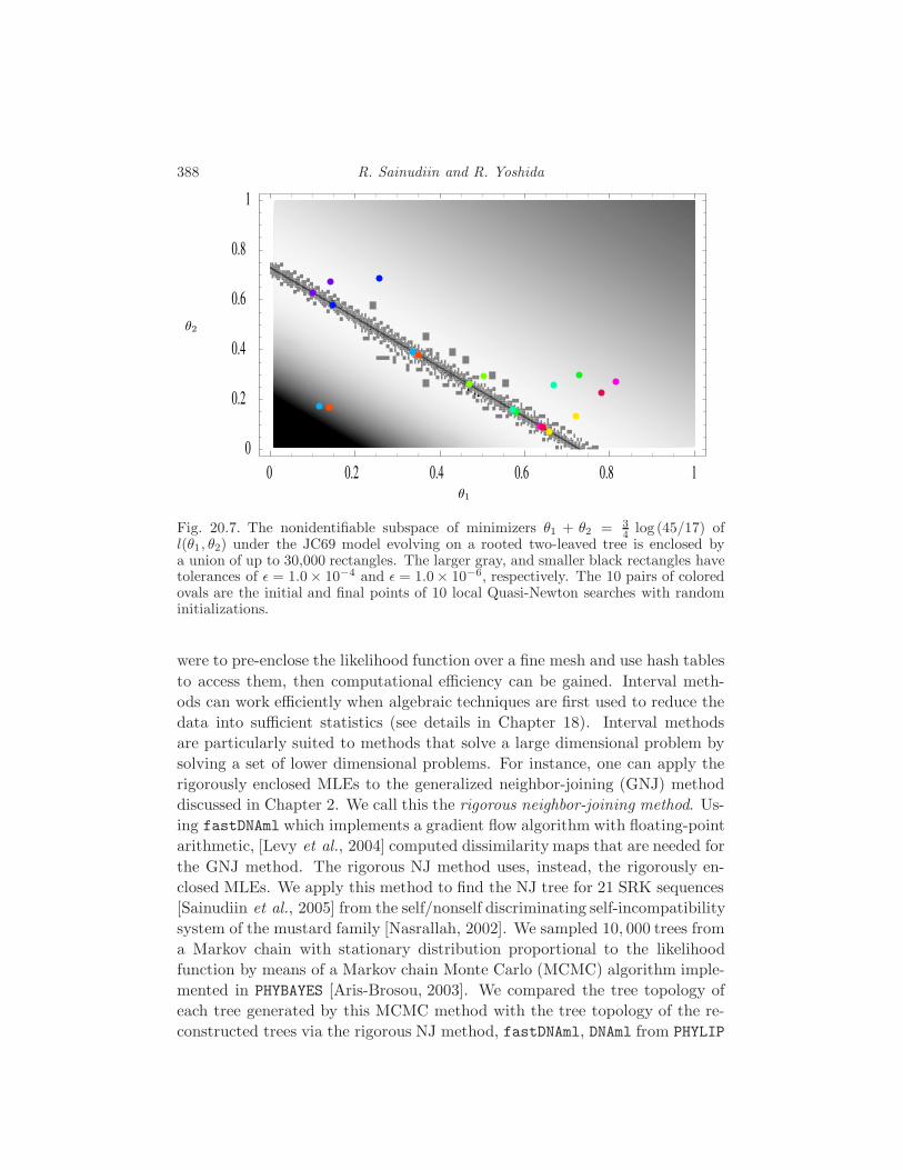
388 R. Sainudiin and R. Yoshida
0 0.2 0.4 0.6 0.8 1
0
0.2
0.4
0.6
0.8
1
θ2
θ1
Fig. 20.7. The nonidentifiable subspace of minimizers θ1 + θ2 = 34
log (45/17) ofl(θ1 , θ2) under the JC69 model evolving on a rooted two-leaved tree is enclosed bya union of up to 30,000 rectangles. The larger gray, and smaller black rectangles havetolerances of ǫ = 1.0× 10⁻⁴ and ǫ = 1.0× 10⁻⁶, respectively. The 10 pairs of coloredovals are the initial and final points of 10 local Quasi-Newton searches with randominitializations.
were to pre-enclose the likelihood function over a fine mesh and use hash tables
to access them, then computational efficiency can be gained. Interval meth-
ods can work efficiently when algebraic techniques are first used to reduce the
data into sufficient statistics (see details in Chapter 18). Interval methods
are particularly suited to methods that solve a large dimensional problem by
solving a set of lower dimensional problems. For instance, one can apply the
rigorously enclosed MLEs to the generalized neighbor-joining (GNJ) method
discussed in Chapter 2. We call this the rigorous neighbor-joining method. Us-
ing fastDNAml which implements a gradient flow algorithm with floating-point
arithmetic, [Levy et al., 2004] computed dissimilarity maps that are needed for
the GNJ method. The rigorous NJ method uses, instead, the rigorously en-
closed MLEs. We apply this method to find the NJ tree for 21 SRK sequences
[Sainudiin et al., 2005] from the self/nonself discriminating self-incompatibility
system of the mustard family [Nasrallah, 2002]. We sampled 10, 000 trees from
a Markov chain with stationary distribution proportional to the likelihood
function by means of a Markov chain Monte Carlo (MCMC) algorithm imple-
mented in PHYBAYES [Aris-Brosou, 2003]. We compared the tree topology of
each tree generated by this MCMC method with the tree topology of the re-
constructed trees via the rigorous NJ method, fastDNAml, DNAml from PHYLIP
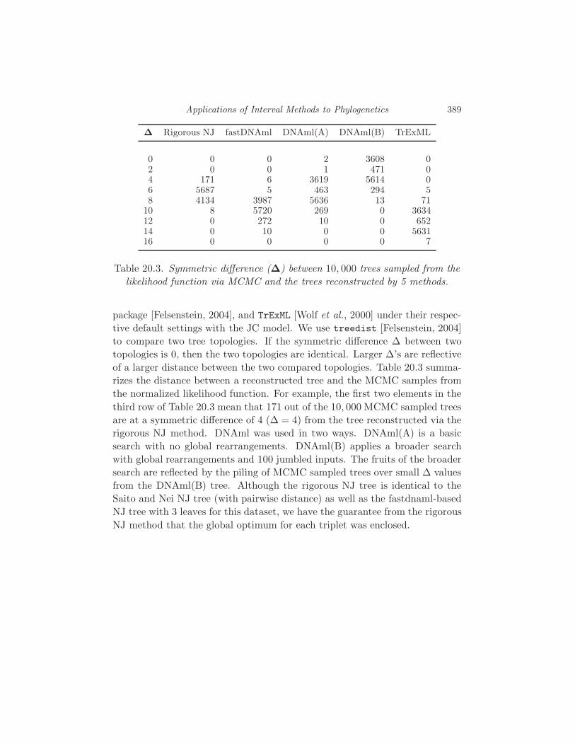
Applications of Interval Methods to Phylogenetics 389
∆ Rigorous NJ fastDNAml DNAml(A) DNAml(B) TrExML
0 0 0 2 3608 02 0 0 1 471 04 171 6 3619 5614 06 5687 5 463 294 58 4134 3987 5636 13 71
10 8 5720 269 0 363412 0 272 10 0 65214 0 10 0 0 563116 0 0 0 0 7
Table 20.3. Symmetric difference (∆) between 10, 000 trees sampled from the
likelihood function via MCMC and the trees reconstructed by 5 methods.
package [Felsenstein, 2004], and TrExML [Wolf et al., 2000] under their respec-
tive default settings with the JC model. We use treedist [Felsenstein, 2004]
to compare two tree topologies. If the symmetric difference ∆ between two
topologies is 0, then the two topologies are identical. Larger ∆’s are reflective
of a larger distance between the two compared topologies. Table 20.3 summa-
rizes the distance between a reconstructed tree and the MCMC samples from
the normalized likelihood function. For example, the first two elements in the
third row of Table 20.3 mean that 171 out of the 10, 000 MCMC sampled trees
are at a symmetric difference of 4 (∆ = 4) from the tree reconstructed via the
rigorous NJ method. DNAml was used in two ways. DNAml(A) is a basic
search with no global rearrangements. DNAml(B) applies a broader search
with global rearrangements and 100 jumbled inputs. The fruits of the broader
search are reflected by the piling of MCMC sampled trees over small ∆ values
from the DNAml(B) tree. Although the rigorous NJ tree is identical to the
Saito and Nei NJ tree (with pairwise distance) as well as the fastdnaml-based
NJ tree with 3 leaves for this dataset, we have the guarantee from the rigorous
NJ method that the global optimum for each triplet was enclosed.

21
Analysis of Point Mutations in Vertebrate Genomes
Jameel Al-Aidroos
Sagi Snir
Using biological sequence from homologs in eight vertebrates of the human
ENCODE regions, we present a concrete example of the estimation of muta-
tion rates in the models of evolution introduced in Chapter 4. We detail the
process of data selection from within a multiple alignment of the vertebrates,
and compare rate estimates for each of the models in the Felsenstein Hierar-
chy of figure 4.6. In the course of the example we also address a standing
problem in vertebrate evolution, namely the resolution of the phylogeny of the
Eutherian orders, and discuss some of the challenges of molecular sequence
analysis in inferring the phylogeny of this subclass. In particular, we consider
the question of the position of the rodents relative to the primates, carnivora
and artiodactyla; a question we affectionately dub the rodent problem.
21.1 Estimating mutation rates
Given an alignment of sequence homologs from various taxa, and a choice of
evolutionary model from among the models in Figure 4.6, we are naturally led
to ask the question,“What tree (with what branch lengths) and what values
of the parameters in the rate matrix for that model are suggested by the
alignment?” One answer to this question, the so-called maximum-likelihood
solution, is, “The tree and rate parameters which maximize the probability
that the given alignment would be generated by the given model.”
There are a number of available software packages which find, to varying de-
grees, this maximum-likelihood solution. For example, for a few of the most re-
strictive models in the Felsenstein hierarchy, the package PHYLIP [Felsenstein, 2004]
will very efficiently search the tree space for the maximum-likelihood tree, and
rate parameters. The commercially available software PAUP* [Swofford, 1998]
effectively searches the tree space, and implements a wider range of models
than PHYLIP. Another package, PAML [Yang, 1997], though it does not reliably
search the tree space, is flexible enough, given a particular tree topology, to
390
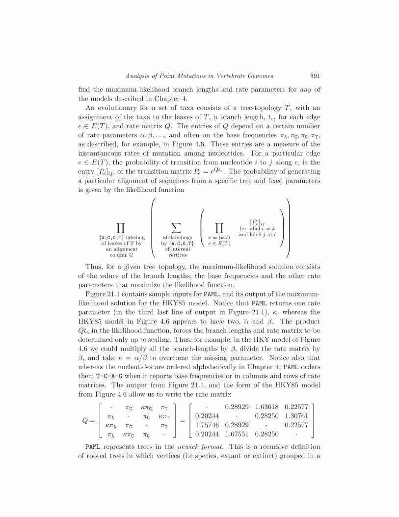
Analysis of Point Mutations in Vertebrate Genomes 391
find the maximum-likelihood branch lengths and rate parameters for any of
the models described in Chapter 4.
An evolutionary for a set of taxa consists of a tree-topology T , with an
assignment of the taxa to the leaves of T , a branch length, te, for each edge
e ∈ E(T ), and rate matrix Q. The entries of Q depend on a certain number
of rate parameters α, β, . . ., and often on the base frequencies πA, πC, πG, πT,
as described, for example, in Figure 4.6. These entries are a measure of the
instantaneous rates of mutation among nucleotides. For a particular edge
e ∈ E(T ), the probability of transition from nucleotide i to j along e, is the
entry [Pe]ij, of the transition matrix Pe = eQte . The probability of generating
a particular alignment of sequences from a specific tree and fixed parameters
is given by the likelihood function
∏
A,C,G,T-labelingof leaves of T by
an alignmentcolumn C
∑
all labelingsby A,C,G,T
of internalvertices
∏
e = (k, l)e ∈ E(T )
[Pe]ijfor label i at kand label j at l
Thus, for a given tree topology, the maximum-likelihood solution consists
of the values of the branch lengths, the base frequencies and the other rate
parameters that maximize the likelihood function.
Figure 21.1 contains sample inputs for PAML, and its output of the maximum-
likelihood solution for the HKY85 model. Notice that PAML returns one rate
parameter (in the third last line of output in Figure 21.1), κ, whereas the
HKY85 model in Figure 4.6 appears to have two, α and β. The product
Qte in the likelihood function, forces the branch lengths and rate matrix to be
determined only up to scaling. Thus, for example, in the HKY model of Figure
4.6 we could multiply all the branch-lengths by β, divide the rate matrix by
β, and take κ = α/β to overcome the missing parameter. Notice also that
whereas the nucleotides are ordered alphabetically in Chapter 4, PAML orders
them T-C-A-G when it reports base frequencies or in columns and rows of rate
matrices. The output from Figure 21.1, and the form of the HKY85 model
from Figure 4.6 allow us to write the rate matrix
Q =
· πC κπG πTπA · πG κπTκπA πC · πTπA κπC πG ·
=
· 0.28929 1.63618 0.22577
0.20244 · 0.28250 1.30761
1.75746 0.28929 · 0.22577
0.20244 1.67551 0.28250 ·
PAML represents trees in the newick format. This is a recursive definition
of rooted trees in which vertices (i.e species, extant or extinct) grouped in a
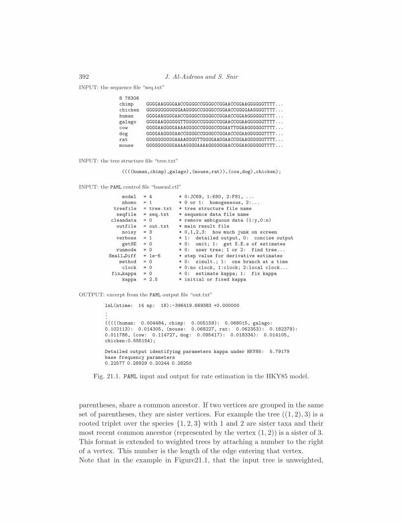
392 J. Al-Aidroos and S. Snir
INPUT: the sequence file “seq.txt”
8 78306chimp GGGGAAGGGGAACCGGGGCCGGGGCCGGAACCGGAAGGGGGGTTTT...chicken GGGGGGGGGGGGAAGGGGCCGGGGCCGGAACCGGGGAAGGGGTTTT...human GGGGAAGGGGAACCGGGGCCGGGGCCGGAACCGGAAGGGGGGTTTT...galago GGGGAAGGGGGGTTGGGGCCGGGGCCGGAACCGGAAGGGGGGTTTT...cow GGGGAAGGGGAAAAGGGGCCGGGGCCGGAATTGGAAGGGGGGTTTT...dog GGGGAAGGGGAACCGGGGCCGGGGCCGGAACCGGAAGGGGGGTTTT...rat GGGGGGGGGGAAAAGGGGTTGGGGAAGGAACCGGAAGGGGGGTTTT...mouse GGGGGGGGGGAAAAGGGGAAAAGGGGGGAACCGGAAGGGGGGTTTT...
INPUT: the tree structure file “tree.txt”
((((human,chimp),galago),(mouse,rat)),(cow,dog),chicken);
INPUT: the PAML control file “baseml.ctl”
model = 4 * 0:JC69, 1:K80, 2:F81, ...nhomo = 1 * 0 or 1: homogeneous, 2:...
treefile = tree.txt * tree structure file nameseqfile = seq.txt * sequence data file name
cleandata = 0 * remove ambiguous data (1:y,0:n)outfile = out.txt * main result file
noisy = 3 * 0,1,2,3: how much junk on screenverbose = 1 * 1: detailed output, 0: concise output
getSE = 0 * 0: omit; 1: get S.E.s of estimatesrunmode = 0 * 0: user tree; 1 or 2: find tree...
Small Diff = 1e-6 * step value for derivative estimatesmethod = 0 * 0: simult.; 1: one branch at a timeclock = 0 * 0:no clock, 1:clock; 2:local clock...
fix kappa = 0 * 0: estimate kappa; 1: fix kappakappa = 2.5 * initial or fixed kappa
OUTPUT: excerpt from the PAML output file “out.txt”
lnL(ntime: 14 np: 18):-396419.669383 +0.000000
.
.
.(((((human: 0.004484, chimp: 0.005159): 0.068015, galago:0.102113): 0.014305, (mouse: 0.068227, rat: 0.062353): 0.182379):0.011786, (cow: 0.114727, dog: 0.095417): 0.018334): 0.014105,chicken:0.555154);
Detailed output identifying parameters kappa under HKY85: 5.79179base frequency parameters0.22577 0.28929 0.20244 0.28250
Fig. 21.1. PAML input and output for rate estimation in the HKY85 model.
parentheses, share a common ancestor. If two vertices are grouped in the same
set of parentheses, they are sister vertices. For example the tree ((1, 2), 3) is a
rooted triplet over the species 1, 2, 3 with 1 and 2 are sister taxa and their
most recent common ancestor (represented by the vertex (1, 2)) is a sister of 3.
This format is extended to weighted trees by attaching a number to the right
of a vertex. This number is the length of the edge entering that vertex.
Note that in the example in Figure21.1, that the input tree is unweighted,
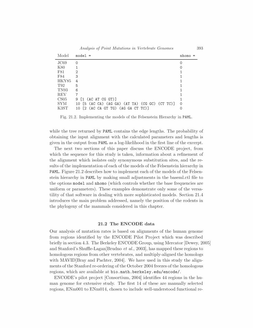
Analysis of Point Mutations in Vertebrate Genomes 393
Model model = nhomo =
JC69 0 0K80 1 0F81 2 1F84 3 1HKY85 4 1T92 5 1TN93 6 1REV 7 1CS05 9 [1 (AC AT CG GT)] 1SYM 10 [5 (AC CA) (AG GA) (AT TA) (CG GC) (CT TC)] 0K3ST 10 [2 (AC CA GT TG) (AG GA CT TC)] 0
Fig. 21.2. Implementing the models of the Felsenstein Hierarchy in PAML.
while the tree returned by PAML contains the edge lengths. The probability of
obtaining the input alignment with the calculated parameters and lengths is
given in the output from PAML as a log-likelihood in the first line of the excerpt.
The next two sections of this paper discuss the ENCODE project, from
which the sequence for this study is taken, information about a refinement of
the alignment which isolates only synonymous substitution sites, and the re-
sults of the implementation of each of the models of the Felsenstein hierarchy in
PAML. Figure 21.2 describes how to implement each of the models of the Felsen-
stein hierarchy in PAML by making small adjustments in the baseml.ctl file to
the options model and nhomo (which controls whether the base frequencies are
uniform or parameters). These examples demonstrate only some of the versa-
tility of that software in dealing with more sophisticated models. Section 21.4
introduces the main problem addressed, namely the position of the rodents in
the phylogeny of the mammals considered in this chapter.
21.2 The ENCODE data
Our analysis of mutation rates is based on alignments of the human genome
from regions identified by the ENCODE Pilot Project which was described
briefly in section 4.3. The Berkeley ENCODE Group, using Mercator [Dewey, 2005]
and Stanford’s Shuffle-Lagan[Brudno et al., 2003], has mapped these regions to
homologous regions from other vertebrates, and multiply-aligned the homologs
with MAVID[Bray and Pachter, 2004]. We have used in this study the align-
ments of the Stanford re-ordering of the October 2004 freezes of the homologous
regions, which are available at bio.math.berkeley.edu/encode/.
ENCODE’s pilot project [Consortium, 2004] identifies 44 regions in the hu-
man genome for extensive study. The first 14 of these are manually selected
regions, ENm001 to ENm014, chosen to include well-understood functional re-

394 J. Al-Aidroos and S. Snir
Manual ENCODE RegionsBin Importance or Expected function
[ENm001] CFTR - Cystic FibrosisENm002 Interleukin Cluster - immune system regulationENm003 Apo Cluster - liver and intestinal functionENm004 region from Chromosome 22ENm005 region from Chromosome 21ENm006 region from Chromosome X[ENm007] region from Chromosome 19ENm008 α-globin - implicated in α-thalassemia (anemia)ENm009 β-globin - implicated in Sickle Cell AnemiaENm010 HOXA Cluster embryonic development: body axis and limb patterning[ENm011] IGF2/H19 - insulin growth factor: growth and early developmentENm012 FOXP2 - language and speech developmentENm013 region from Chromosome 7 - selected to balance stratificationENm014 region from Chromosome 7 - selected to balance stratification
Random ENCODE Regionsdensity of density ofconserved genic basesnon-exonic low medium highbases (0-50%-ile) (60-80%-ile) (80-100%-ile)
low(0-50%-ile)
ENr111, [ENr112]ENr113, ENr114
ENr121, ENr122ENr123
ENr131, ENr132ENr133
medium(50-80%-ile)
ENr211, ENr212[ENr213]
ENr221, ENr222ENr223
ENr231, ENr232ENr233
high(80-100%-ile)
ENr311, [ENr312]ENr313
ENr321, ENr322ENr323, ENr324
ENr331, ENr332ENr333,[ENr334]
Fig. 21.3. Summary of the manual and random ENCODE regions. [..] denotes aregion that was not considered in this study because a homolog was missing for atleast one of the seven other vertebrates at the time the data was generated.
gions of the genome. For example, ENm001 contains the gene CFTR, associ-
ated with cystic fibrosis, which has been studied extensively since its discovery
in 1989. The remaining 30 regions, the so-called “random” regions, were cho-
sen pseudo-randomly to represent varying degrees of non-exonic conservation
with respect to orthologous sequence from the mouse genome, and varying de-
grees of gene density. Figure 21.3 describes the manual and random ENCODE
regions.
A primary goal of the Berkeley ENCODE Group is to generate mappings
from the human genome in the ENCODE regions to homologous regions in
assemblies of sequence from other vertebrates, and to align the homologs. Such
alignments have been generated for each ENCODE region, although the set of
taxa in which homologs have been identified varies from region to region. In
this study, we restricted our attention to the eight vertebrates human (Homo
sapiens), galago monkey (Otolemur garnettii), chimp (Pan troglodytes), rat
(Rattus norvegicus), mouse (Mus musculus), dog (Canis familiaris), cow (Bos
taurus) and chicken (Gallus gallus), and considered only the 37 ENCODE
regions which, at the time we generated data, had alignments of homologs for

Analysis of Point Mutations in Vertebrate Genomes 395
all eight taxa. In Figure 21.3, the regions that appear in square braces are those
for which the homolog was missing for at least one of our eight vertebrates,
and which were not considered.
21.3 Synonymous substitutions
Starting with the MAVID alignment of the homologs of the human ENCODE
regions, we refined the alignment by isolating only those columns corresponding
to synonymous substitution sites in exons. In this section we define synony-
mous substitution, and describe the process for identifying these columns of
the alignment.
Recall from Table 4.1 in Chapter 4 that every amino acid is coded by a
sequence of three nucleotides, called a codon. As there are four (types of)
nucleotides, this scheme allows for 43 = 64 different codons. However, since
there are only twenty amino acids, the above implies that some amino acids are
encoded by a few different codons, giving some redundancy to the amino acid
coding scheme. Nucleotide mutations in the gene (which necessarily change
the codons in the gene) are divided into three types, depending on what amino
acid is encoded by the new codon:
(i) synonymous mutations: mutations that, although they alter a particular
codon, they do not alter the encoded amino acid.
(ii) missense mutations: mutations that alter the codon so as to produce
an different amino acid.
(iii) nonsense mutations: mutations that change a codon that encodes an
amino acid into one of the STOP codons (TAA, TAG, or TGA).
Because synonymous mutations do not alter the amino acid, they do not alter
the protein. Such mutations produce no functional changes, and are thus con-
sidered to be free from selective pressure. By removing the selective pressure,
we restrict our attention to those sites whose mutation is more likely to be-
have according to a random Markov process. Furthermore, by isolating these
synonymous substitution sites, we impose a level of homogeneity on the data.
For example, although PAML implements models that allow for the rate matrix
to vary among sites, we believe that by selecting the neutral mutation sites,
we substantially reduce the need for this introduction of extra parameters into
the models.
The procedure for refinement of the data consisted of mapping annota-
tions of human genes to the alignment, and identifying triples of columns
containing synonymous codons. For each of the 37 ENCODE regions, we
identified the manually verified (refSeq) annotations of genes in that re-
gion by consulting the refGene table in the UCSC annotation database

396 J. Al-Aidroos and S. Snir
a.a. GlnMetGlnGlnLeuGlnGlnGlnGlnHisLeuLeu...LeuGln...GlnGlyLeuIle
human CAGATGCAACAACTCCAGCAGCAGCAGCATCTGCTCAGCCTTCAGCGTCAGGGACTCATCgalago CAGATGCAACAACTCCAGCAGCAGCAGCATCTGCTCAGCCTTCAGCGTCAGGGACTCATCmouse CAAATGCAGCAGCTACAGCAGCAACAACATCTGCTCAGCCTTCAGCGCCAGGGCCTCATC
rat CAGATGCAGCAACTACAGCAGCAGCAGCATCTGCTCAGCCTTCAGTGTCAGGGCCTCATCcow CAGATGCAACAACTCCAGCAGCAGCAGCATCTGCTCAGCCTTCAGCGTCAGGGACTCATC
chicken CAGATGCAACAACTTCAGCAGCAGCAACATCTGCTGAACCTTCAGCGTCAGGGACTCATTchimp CAGATGCAACAACTCCAGCAGCAGCAGCATCTGCTCAGCCTTCAGCGTCAGGGACTCATC
dog CAGATGCAACAACTCCAGCAGCAGCAGCATCTGCTCAGCCTTCAGCGTCAGGGACTCATC
..*.....*..*..*..*..*..*..*..*..*..*.....*..*.....*..*..*..*123123123123123123123123123123123123123123123123123123123123
Fig. 21.4. Excerpt of alignment from FOXP2 (RefSeq annot. NM 148900) in ENm012.The top row indicates the amino acid translation of the codon (where all there isagreement among all the taxa). The stars denote columns corresponding to the thirdpositions in codons all coding for the same amino acid. The bottom row indicates theframe dictated by the human gene annotation, where 1 denotes the first position in acodon.
(hgdownload.cse.ucsc.edu/downloads.html). For each gene in the region,
we mapped the annotation of its coding region to the MAVID alignment, and
extracted the relevant columns. Below each codon triple in the human se-
quence, we identified the amino acids encoded by the triple in each of the
homologs. We automatically discarded all triples which contained gaps in any
of the homologs, and extracted the third column from each triple in which
each homolog’s codon encoded the amino acid in the human sequence. We
note here that because of gaps in the alignment and because we use only the
frame of the human annotation to identify coding triples, it is possible that
some sites chosen correspond to a second or third position in a codon of one
of the other vertebrates. The high degree of conservation in the aligned ex-
ons, and the stringent requirement of agreement in the preceding two columns,
however, meant that extracted columns were very unlikely to suffer from this
fault; a visual inspection of the alignments revealed that extracted columns
very reliably consisted of third positions. An excerpt of the alignment from
the speech and language development gene, FOXP2, is given in Figure 21.4.
With the refined sequence data in hand we used PAML to find the maximum-
likelihood solutions for the rate parameters, base frequencies and branch
lengths. However, as was indicated in the introductory chapter, PAML does
not reliably search the tree space, so we restricted ourselves to only the two
trees in Figure 21.7, namely the tree tree (that is, the actual tree representing
the evolutionary history of those species), and the maximum likelihood tree
(The tree attaining the biggest likelihood under all models studied). The rate
Analysis of Point Mutations in Vertebrate Genomes 397
Fig. 21.5. The Felsenstein Hierarchy for the ML Tree.
Fig. 21.6. The Felsenstein Hierarchy for the True Tree.
matrices and log-likelihoods for each model are displayed in Figures 21.5 and
21.6.
21.4 The rodent problem
Rodents have the special characteristic that although their molecular informa-
tion closely resembles that of the primates, they exhibit very different mor-
phological features. This discrepancy has attracted a lot of attention and has
formed the basis of much research.
In this section we point out the phenomenon that current tree reconstruc-
tion methods misplace the two rodents mouse and rat on the tree, with
respect to other mammals. The real phylogenetic tree describing the evo-
lution of the taxa in this study is agreed among most of the evolution-
ary biologists nowadays. It is supported by either fossil records or molecu-
lar data ([Madsen et al., 2001, Murphy et al., 2001, Phillips and Penny, 2003,
Lin et al., 2002, Schmitz and Zischler, 2003] to mention a few). In that tree
(see Figure 21.7 up), we have the primate clade, composed of the siblings
human and chimpanzee and then the galago as an outgroup to these two.
The rodents clade mouse and rat, is a sister group to the primates and an
artiodactyls-carnivores clade is an outgroup to the former species. By using
the chicken as an outgroup to all these, we get a rooting of the tree. How-
ever, the currently available phylogenetic reconstruction methods, regardless
of the evolutionary model, misplace the rodents and put them as an outgroup
to the primates and artiodactyls-carnivores (see Figure 21.7 down). A partial
explanation to this phenomenon is given by the fact that rodents have shorter
generation time. This causes the rate of synonymous substitutions in the ro-
dents to be 2.0 times faster than in human and the rate of non-synonymous
substitutions to be 1.3 times faster [Wu and Li, 1985].
This question of rodents divergence time (and the relative location of
this event on the phylogeny) has a long history and is still gaining a
lot of popularity with the increasing availability of complete mammalian
genomes (e.g. [International Human Genome Sequencing Consortium, 2001,
Waterston et al., 2002, Hillier et al., 2004, Gibbs et al., 2004]). Recent works
( [Adkins et al., 2001, Thomas et al., 2003]) have also addressed the question
that few methods fail to estimate correctly this event. [Adkins et al., 2001]
addressed the question of monophyly of the rodents order and noticed that
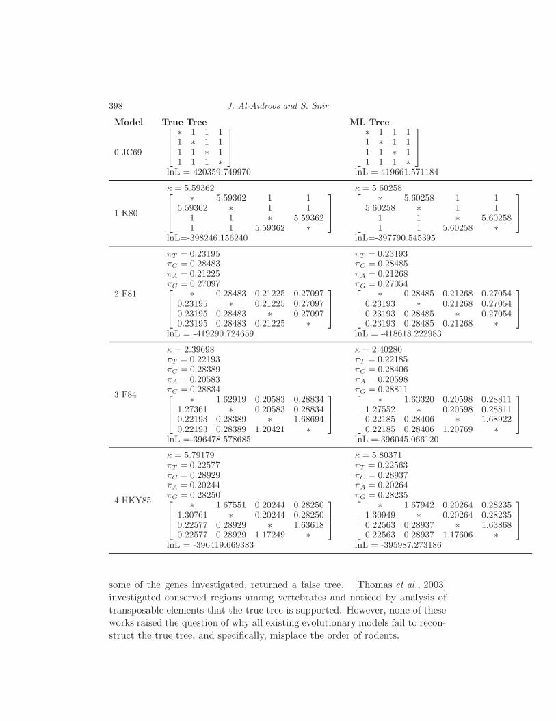
398 J. Al-Aidroos and S. Snir
Model True Tree ML Tree
0 JC69
∗ 1 1 11 ∗ 1 11 1 ∗ 11 1 1 ∗
lnL =-420359.749970
∗ 1 1 11 ∗ 1 11 1 ∗ 11 1 1 ∗
lnL =-419661.571184
1 K80
κ = 5.59362
∗ 5.59362 1 15.59362 ∗ 1 1
1 1 ∗ 5.593621 1 5.59362 ∗
lnL=-398246.156240
κ = 5.60258
∗ 5.60258 1 15.60258 ∗ 1 1
1 1 ∗ 5.602581 1 5.60258 ∗
lnL=-397790.545395
2 F81
πT = 0.23195πC = 0.28483πA = 0.21225πG = 0.27097
∗ 0.28483 0.21225 0.270970.23195 ∗ 0.21225 0.270970.23195 0.28483 ∗ 0.270970.23195 0.28483 0.21225 ∗
lnL = -419290.724659
πT = 0.23193πC = 0.28485πA = 0.21268πG = 0.27054
∗ 0.28485 0.21268 0.270540.23193 ∗ 0.21268 0.270540.23193 0.28485 ∗ 0.270540.23193 0.28485 0.21268 ∗
lnL = -418618.222983
3 F84
κ = 2.39698πT = 0.22193πC = 0.28389πA = 0.20583πG = 0.28834
∗ 1.62919 0.20583 0.288341.27361 ∗ 0.20583 0.288340.22193 0.28389 ∗ 1.686940.22193 0.28389 1.20421 ∗
lnL =-396478.578685
κ = 2.40280πT = 0.22185πC = 0.28406πA = 0.20598πG = 0.28811
∗ 1.63320 0.20598 0.288111.27552 ∗ 0.20598 0.288110.22185 0.28406 ∗ 1.689220.22185 0.28406 1.20769 ∗
lnL =-396045.066120
4 HKY85
κ = 5.79179πT = 0.22577πC = 0.28929πA = 0.20244πG = 0.28250
∗ 1.67551 0.20244 0.282501.30761 ∗ 0.20244 0.282500.22577 0.28929 ∗ 1.636180.22577 0.28929 1.17249 ∗
lnL = -396419.669383
κ = 5.80371πT = 0.22563πC = 0.28937πA = 0.20264πG = 0.28235
∗ 1.67942 0.20264 0.282351.30949 ∗ 0.20264 0.282350.22563 0.28937 ∗ 1.638680.22563 0.28937 1.17606 ∗
lnL = -395987.273186
some of the genes investigated, returned a false tree. [Thomas et al., 2003]
investigated conserved regions among vertebrates and noticed by analysis of
transposable elements that the true tree is supported. However, none of these
works raised the question of why all existing evolutionary models fail to recon-
struct the true tree, and specifically, misplace the order of rodents.

Analysis of Point Mutations in Vertebrate Genomes 399
5 T92
κ =πT =πC =πA =πG =
∗ πC πA πG
πT ∗ πA πG
πT πC ∗ πG
πT πC πA ∗
lnL =
πT =πC =πA =πG =
∗ πC πA πG
πT ∗ πA πG
πT πC ∗ πG
πT πC πA ∗
lnL =
6 TN93
κ1 = 6.29360κ2 = 5.28772πT = 0.21984πC = 0.28271πA = 0.20870πG = 0.28874
∗ 1.77926 0.20870 0.288741.38359 ∗ 0.20870 0.288740.21984 0.28271 ∗ 1.526780.21984 0.28271 1.10355 ∗
lnL =-396308.224349
κ1 = 6.29927κ2 = 5.30517πT = 0.21979πC = 0.28288πA = 0.20884πG = 0.28849
∗ 1.78194 0.20884 0.288491.38452 ∗ 0.20884 0.288490.21979 0.28288 ∗ 1.530490.21979 0.28288 1.10793 ∗
lnL =-395879.760438
7 REV
∗ 0.928553 0.153082 0.1142290.719295 ∗ 0.138117 0.1171850.167314 0.194874 ∗ 0.8227510.084580 0.112011 0.557377 ∗
lnL =-395649.076601
∗ 0.928911 0.155345 0.1130080.718400 ∗ 0.137595 0.1162500.169773 0.194438 ∗ 0.8242700.083624 0.111230 0.558110 ∗
lnL = -395194.825177
9 CS05
−1.126077 0.873315 0.105515 0.1472470.681559 −0.934321 0.105515 0.1472470.117676 0.150784 −1.121289 0.8528280.117676 0.150784 0.611124 −0.879585
lnL =-396419.669383
−1.126393 0.873994 0.1054580.681474 −0.933873 0.1054580.117421 0.150592 −1.1208140.117421 0.150592 0.612049
lnL = -395987.273185
10 SYM
−1.066465 0.809931 0.159339 0.0971940.809931 −1.087021 0.158949 0.1181410.159339 0.158949 −0.974734 0.6564460.097194 0.118141 0.656446 −0.871780
lnL =-397702.025844
−1.067056 0.809476 0.1614380.809476 −1.085413 0.1584480.161438 0.158448 −0.9768930.096143 0.117489 0.657007
lnL = -397237.324766
11 K3ST
−1.000000 0.736581 0.135559 0.1278600.736581 −1.000000 0.127860 0.1355590.135559 0.127860 −1.000000 0.7365810.127860 0.135559 0.736581 −1.000000
lnL =-395649.076601
−1.000000 0.736880 0.1359500.736880 −1.000000 0.1271700.135950 0.127170 −1.0000000.127170 0.135950 0.736880
lnL = -398241.937632
A common feature of many of the most popular models used to reconstruct
the evolutionary tree is the assumption of a constant rate matrix along all
branches. This leaves the time as the only free parameter between the dif-
ferent branches of the tree. As a consequence, it causes distortion in the
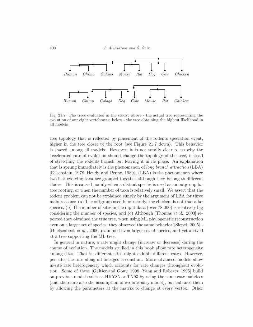
400 J. Al-Aidroos and S. Snir
b
b
bb
b
b
Humanb
Chimpb
Galago
b
b
Mouseb
Rat
b
b
Dogb
Cowb
Chicken
b
bb
bb
b
Humanb
Chimpb
Galago
b
b
Dogb
Cow
b
b
Mouseb
Ratb
Chicken
Fig. 21.7. The trees evaluated in the study: above - the actual tree representing theevolution of our eight vertebrates; below - the tree obtaining the highest likelihood inall models
tree topology that is reflected by placement of the rodents speciation event,
higher in the tree closer to the root (see Figure 21.7 down). This behavior
is shared among all models. However, it is not totally clear to us why the
accelerated rate of evolution should change the topology of the tree, instead
of stretching the rodents branch but leaving it in its place. An explanation
that is sprung immediately is the phenomenon of long branch attraction (LBA)
[Felsenstein, 1978, Hendy and Penny, 1989]. (LBA) is the phenomenon where
two fast evolving taxa are grouped together although they belong to different
clades. This is caused mainly when a distant species is used as an outgroup for
tree rooting, or when the number of taxa is relatively small. We assert that the
rodent problem can not be explained simply by the argument of LBA for three
main reasons: (a) The outgroup used in our study, the chicken, is not that a far
species, (b) The number of sites in the input data (over 78,000) is relatively big
considering the number of species, and (c) Although [Thomas et al., 2003] re-
ported they obtained the true tree, when using ML phylogenetic reconstruction
even on a larger set of species, they observed the same behavior([Siepel, 2005]).
[Huelsenbeck et al., 2000] examined even larger set of species, and yet arrived
at a tree supporting the ML tree.
In general in nature, a rate might change (increase or decrease) during the
course of evolution. The models studied in this book allow rate heterogeneity
among sites. That is, different sites might exhibit different rates. However,
per site, the rate along all lineages is constant. More advanced models allow
in-site rate heterogeneity which accounts for rate changes throughout evolu-
tion. Some of these [Galtier and Gouy, 1998, Yang and Roberts, 1995] build
on previous models such as HKY85 or TN93 by using the same rate matrices
(and therefore also the assumption of evolutionary model), but enhance them
by allowing the parameters at the matrix to change at every vertex. Other
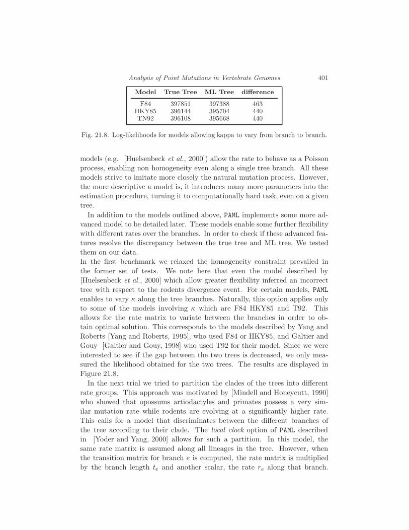
Analysis of Point Mutations in Vertebrate Genomes 401
Model True Tree ML Tree difference
F84 397851 397388 463HKY85 396144 395704 440TN92 396108 395668 440
Fig. 21.8. Log-likelihoods for models allowing kappa to vary from branch to branch.
models (e.g. [Huelsenbeck et al., 2000]) allow the rate to behave as a Poisson
process, enabling non homogeneity even along a single tree branch. All these
models strive to imitate more closely the natural mutation process. However,
the more descriptive a model is, it introduces many more parameters into the
estimation procedure, turning it to computationally hard task, even on a given
tree.
In addition to the models outlined above, PAML implements some more ad-
vanced model to be detailed later. These models enable some further flexibility
with different rates over the branches. In order to check if these advanced fea-
tures resolve the discrepancy between the true tree and ML tree, We tested
them on our data.
In the first benchmark we relaxed the homogeneity constraint prevailed in
the former set of tests. We note here that even the model described by
[Huelsenbeck et al., 2000] which allow greater flexibility inferred an incorrect
tree with respect to the rodents divergence event. For certain models, PAML
enables to vary κ along the tree branches. Naturally, this option applies only
to some of the models involving κ which are F84 HKY85 and T92. This
allows for the rate matrix to variate between the branches in order to ob-
tain optimal solution. This corresponds to the models described by Yang and
Roberts [Yang and Roberts, 1995], who used F84 or HKY85, and Galtier and
Gouy [Galtier and Gouy, 1998] who used T92 for their model. Since we were
interested to see if the gap between the two trees is decreased, we only mea-
sured the likelihood obtained for the two trees. The results are displayed in
Figure 21.8.
In the next trial we tried to partition the clades of the trees into different
rate groups. This approach was motivated by [Mindell and Honeycutt, 1990]
who showed that opossums artiodactyles and primates possess a very sim-
ilar mutation rate while rodents are evolving at a significantly higher rate.
This calls for a model that discriminates between the different branches of
the tree according to their clade. The local clock option of PAML described
in [Yoder and Yang, 2000] allows for such a partition. In this model, the
same rate matrix is assumed along all lineages in the tree. However, when
the transition matrix for branch e is computed, the rate matrix is multiplied
by the branch length te and another scalar, the rate re along that branch.

402 J. Al-Aidroos and S. Snir
Model True Tree ML Tree difference
HKY85 396604 396339 265T92 396711 396443 268
TN93 396493 396232 261REV 395834 395559 275
UNREST 395646 395365 281
Fig. 21.9. Log-likelihoods for models using local clock option.
This provides the model with the property that the tree inferred satisfies
the molecular clock property, while allowing rate heterogeneity. Indeed in
[Douzery E. J. P. and D., 2003] this model was used with very similar group-
ing (as the set of taxa was different) for the study of the discrepancy between
fossil calibration and estimation based on molecular data. However, in their
study, only the true tree was considered as the different goals were posed. , we
the leaves into 3 groups:
(i) The chicken clade (which comprise the branch from the root to the
chicken)
(ii) The rodents clade (comprises all edge joining the ancestral rodent)
(iii) All the rest
the results obtained under this model are depicted in Figure 21.9. It can be
seen that under this model the difference in the log likelihood is diminished,
nevertheless, still the ML tree prevails.
22
Ultra-Conserved Elements in Vertebrate and FlyGenomes
Mathias Drton
Nicholas Eriksson
Garmay Leung
Ultra-conserved elements in multiple aligned genomes consist of consecutive
nucleotides that are in perfect agreement across all the genomes. For aligned
vertebrate and aligned fly genomes, we give descriptive statistics of ultra-
conserved elements, explain their biological relevance, and calculate the prob-
ability of occurrence of ultra-conserved elements using statistical models.
22.1 The Data
Our analyses of ultra-conserved elements are based on multiple sequence align-
ments produced by MAVID [Bray and Pachter, 2004]. Prior to the alignment
of multiple genomes, homology mappings (from Mercator [Dewey, 2005]) bin
together genomic regions that are anchored together by homologous exons. A
multiple sequence alignment is then produced for each of these alignment bins.
MAVID is a global multiple alignment program, and therefore homologous re-
gions with more than one homologous hit to another genome may not be found
aligned together.
The vertebrate dataset consists of 10,279 bins over 9 genomes: zebra
fish (Danio rerio), fugu fish (Takifugu rubripes), puffer fish (Tetraodon ni-
groviridis), dog (Canis familiaris), human (Homo sapiens), chimp (Pan troglo-
gytes), mouse (Mus musculus), rat (Rattus norvegicus) and chicken (Gallus
gallus). The genome sizes range from 260 Mbp (million base pairs) to 4.2 Gbp
(billion base pairs). A total of 4,368 bins (42.5%) contain alignments across
all 9 species. The evolutionary relationships between these species (which first
diverged about 450 million years ago) are shown in Figure 22.1.
The fruit fly dataset consists of 8 Drosophila genomes: D. melanogaster, D.
simulans, D. yakuba, D. erecta, D. ananassae, D. pseudoobscura, D. virilis and
D. mojavensis. Each of these genomes consists of 114 to 177 Mbp, and 2,985 of
the 3,731 alignment bins (80.0%) contain all 8 species, indicative of a smaller
403
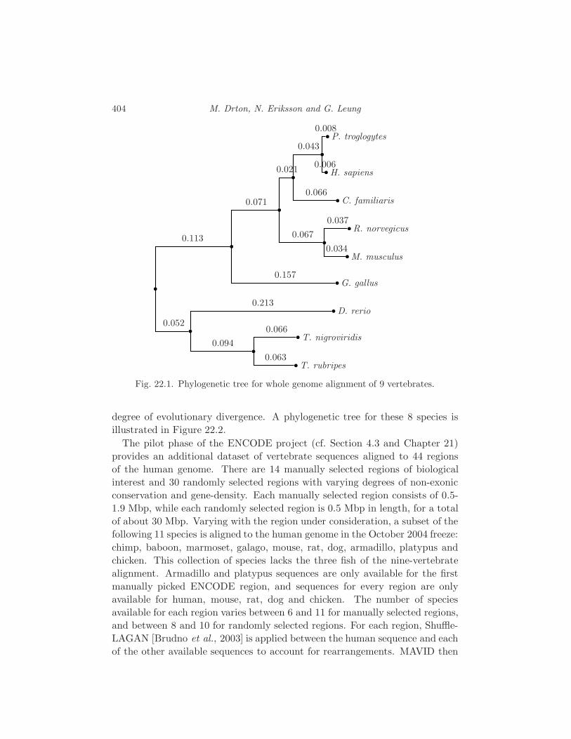
404 M. Drton, N. Eriksson and G. Leung
b
b
0.113
b
0.071
b
0.021
b
0.043
bP. troglogytes0.008
bH. sapiens0.006
bC. familiaris0.066
b
0.067bR. norvegicus
0.037
bM. musculus0.034
bG. gallus0.157
b
0.052
bD. rerio0.213
b
0.094bT. nigroviridis
0.066
bT. rubripes0.063
Fig. 22.1. Phylogenetic tree for whole genome alignment of 9 vertebrates.
degree of evolutionary divergence. A phylogenetic tree for these 8 species is
illustrated in Figure 22.2.
The pilot phase of the ENCODE project (cf. Section 4.3 and Chapter 21)
provides an additional dataset of vertebrate sequences aligned to 44 regions
of the human genome. There are 14 manually selected regions of biological
interest and 30 randomly selected regions with varying degrees of non-exonic
conservation and gene-density. Each manually selected region consists of 0.5-
1.9 Mbp, while each randomly selected region is 0.5 Mbp in length, for a total
of about 30 Mbp. Varying with the region under consideration, a subset of the
following 11 species is aligned to the human genome in the October 2004 freeze:
chimp, baboon, marmoset, galago, mouse, rat, dog, armadillo, platypus and
chicken. This collection of species lacks the three fish of the nine-vertebrate
alignment. Armadillo and platypus sequences are only available for the first
manually picked ENCODE region, and sequences for every region are only
available for human, mouse, rat, dog and chicken. The number of species
available for each region varies between 6 and 11 for manually selected regions,
and between 8 and 10 for randomly selected regions. For each region, Shuffle-
LAGAN [Brudno et al., 2003] is applied between the human sequence and each
of the other available sequences to account for rearrangements. MAVID then
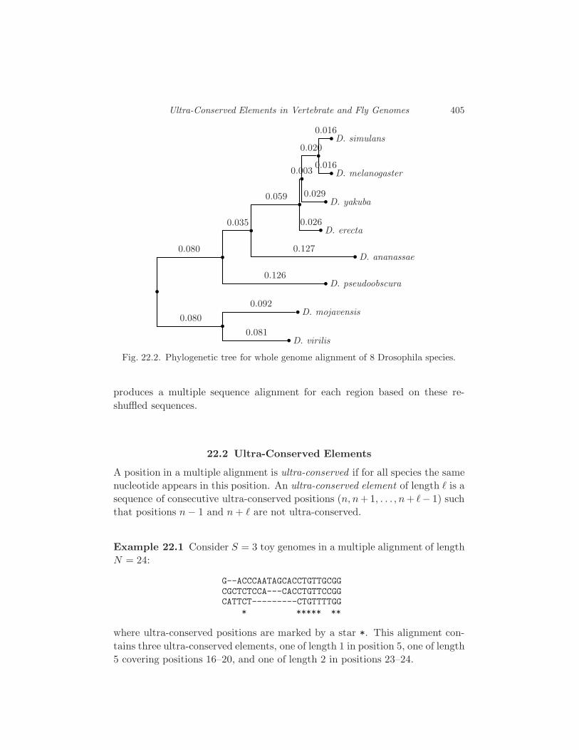
Ultra-Conserved Elements in Vertebrate and Fly Genomes 405
b
b
0.080
b
0.035
b
0.059
b
0.003
b
0.020
bD. simulans0.016
bD. melanogaster0.016
bD. yakuba0.029
bD. erecta0.026
bD. ananassae0.127
bD. pseudoobscura0.126
b
0.080bD. mojavensis
0.092
bD. virilis0.081
Fig. 22.2. Phylogenetic tree for whole genome alignment of 8 Drosophila species.
produces a multiple sequence alignment for each region based on these re-
shuffled sequences.
22.2 Ultra-Conserved Elements
A position in a multiple alignment is ultra-conserved if for all species the same
nucleotide appears in this position. An ultra-conserved element of length ℓ is a
sequence of consecutive ultra-conserved positions (n, n+ 1, . . . , n+ ℓ− 1) such
that positions n− 1 and n+ ℓ are not ultra-conserved.
Example 22.1 Consider S = 3 toy genomes in a multiple alignment of length
N = 24:
G--ACCCAATAGCACCTGTTGCGGCGCTCTCCA---CACCTGTTCCGGCATTCT---------CTGTTTTGG
* ***** **
where ultra-conserved positions are marked by a star *. This alignment con-
tains three ultra-conserved elements, one of length 1 in position 5, one of length
5 covering positions 16–20, and one of length 2 in positions 23–24.
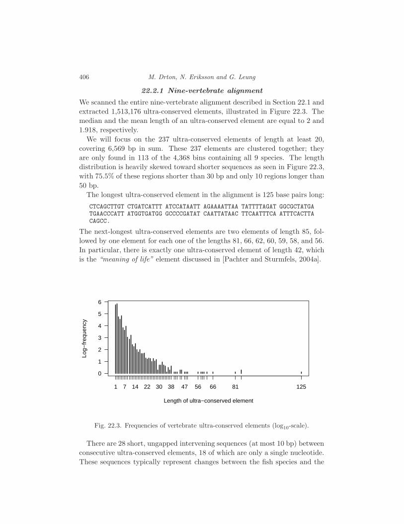
406 M. Drton, N. Eriksson and G. Leung
22.2.1 Nine-vertebrate alignment
We scanned the entire nine-vertebrate alignment described in Section 22.1 and
extracted 1,513,176 ultra-conserved elements, illustrated in Figure 22.3. The
median and the mean length of an ultra-conserved element are equal to 2 and
1.918, respectively.
We will focus on the 237 ultra-conserved elements of length at least 20,
covering 6,569 bp in sum. These 237 elements are clustered together; they
are only found in 113 of the 4,368 bins containing all 9 species. The length
distribution is heavily skewed toward shorter sequences as seen in Figure 22.3,
with 75.5% of these regions shorter than 30 bp and only 10 regions longer than
50 bp.
The longest ultra-conserved element in the alignment is 125 base pairs long:
CTCAGCTTGT CTGATCATTT ATCCATAATT AGAAAATTAA TATTTTAGAT GGCGCTATGATGAACCCATT ATGGTGATGG GCCCCGATAT CAATTATAAC TTCAATTTCA ATTTCACTTACAGCC.
The next-longest ultra-conserved elements are two elements of length 85, fol-
lowed by one element for each one of the lengths 81, 66, 62, 60, 59, 58, and 56.
In particular, there is exactly one ultra-conserved element of length 42, which
is the “meaning of life” element discussed in [Pachter and Sturmfels, 2004a].
0
1
2
3
4
5
6
Length of ultra−conserved element
Log−
freq
uenc
y
1 7 14 22 30 38 47 56 66 81 125
Fig. 22.3. Frequencies of vertebrate ultra-conserved elements (log10-scale).
There are 28 short, ungapped intervening sequences (at most 10 bp) between
consecutive ultra-conserved elements, 18 of which are only a single nucleotide.
These sequences typically represent changes between the fish species and the

Ultra-Conserved Elements in Vertebrate and Fly Genomes 407
other vertebrates. Stringing together elements separated by less than 10 bases
would reduce the number of ultra-conserved elements to 209, increase the base
coverage to 6,636 bp, and bring the total number of regions greater than 50
bp in length to 26.
In the human genome, the GC-ratio (proportion of G and C among all nu-
cleotides) is 41.0%. The ultra-conserved elements are slightly more AT-rich;
for the 237 elements of length 20 or longer, the GC-ratio is 35.8%. Similar
AT-richness is, however, also present in some parts of the alignment that do
not contain ultra-conserved elements, which constitutes one of the reasons why
our attempts at predicting ultra-conserved elements from single species data
using a hidden Markov model were unsuccessful.
22.2.2 ENCODE alignment
The 44 ENCODE regions contain 139,043 ultra-conserved elements, 524 of
which are longer than 20 base pairs. These long elements cover 17,823 bp. By
base coverage, 73.5% of the long elements are found in the manually chosen
regions. The longest one is in region ENm012, of length 169 and consists of the
DNA sequence:
AAGTGCTTTG TGAGTTTGTC ACCAATGATA ATTTAGATAG AGGCTCATTA CTGAACATCACAACACTTTA AAAACCTTTC GCCTTCATAC AGGAGAATAA AGGACTATTT TAATGGCAAGGTTCTTTTGT GTTCCACTGA AAAATTCAAT CAAGACAAAA CCTCATTGA.
It does not contain a subsequence of length 20 or longer that is ultra-conserved
in the nine-vertebrate alignment, however, the 169 base pairs are also ultra-
conserved in the nine-vertebrate alignment if one excludes the three fish from
consideration. The only overlap between the nine-vertebrate and ENCODE
ultra-conserved elements occurs in the regions ENm012 and ENm005, where there
are 3 elements that are extensions of ultra-conserved elements in the nine-
vertebrate alignment.
Table 22.1 shows the number of species aligned in the 44 ENCODE align-
ments and the respective five longest ultra-conserved elements that are of
length 20 or larger. Omitted randomly selected regions do not contain any
ultra-conserved elements of length at least 20.
22.2.3 Eight-Drosophila alignment
There are 5,591,547 ultra-conserved elements in the Drosophila dataset, with
1,705 elements at least 50 bp long and the longest of length 209 bp. We
focus on the 255 Drosophila ultra-conserved elements of length of at least 75
bp, covering 23,567 bp total. These regions are also found clustered together,
occurring over 163 bins out of the 2,985 bins with all 8 species aligned together.
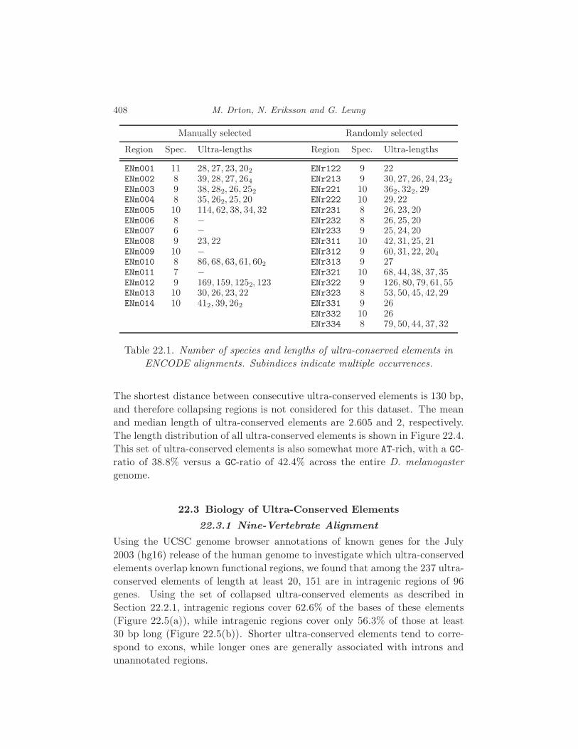
408 M. Drton, N. Eriksson and G. Leung
Manually selected Randomly selected
Region Spec. Ultra-lengths Region Spec. Ultra-lengths
ENm001 11 28, 27, 23, 202 ENr122 9 22ENm002 8 39, 28, 27, 264 ENr213 9 30, 27, 26, 24, 232
ENm003 9 38, 282, 26, 252 ENr221 10 362, 322, 29ENm004 8 35, 262, 25, 20 ENr222 10 29, 22ENm005 10 114, 62, 38, 34, 32 ENr231 8 26, 23, 20ENm006 8 − ENr232 8 26, 25, 20ENm007 6 − ENr233 9 25, 24, 20ENm008 9 23, 22 ENr311 10 42, 31, 25, 21ENm009 10 − ENr312 9 60, 31, 22, 204
ENm010 8 86, 68, 63, 61, 602 ENr313 9 27ENm011 7 − ENr321 10 68, 44, 38, 37, 35ENm012 9 169, 159, 1252, 123 ENr322 9 126, 80, 79, 61, 55ENm013 10 30, 26, 23, 22 ENr323 8 53, 50, 45, 42, 29ENm014 10 412, 39, 262 ENr331 9 26
ENr332 10 26ENr334 8 79, 50, 44, 37, 32
Table 22.1. Number of species and lengths of ultra-conserved elements in
ENCODE alignments. Subindices indicate multiple occurrences.
The shortest distance between consecutive ultra-conserved elements is 130 bp,
and therefore collapsing regions is not considered for this dataset. The mean
and median length of ultra-conserved elements are 2.605 and 2, respectively.
The length distribution of all ultra-conserved elements is shown in Figure 22.4.
This set of ultra-conserved elements is also somewhat more AT-rich, with a GC-
ratio of 38.8% versus a GC-ratio of 42.4% across the entire D. melanogaster
genome.
22.3 Biology of Ultra-Conserved Elements
22.3.1 Nine-Vertebrate Alignment
Using the UCSC genome browser annotations of known genes for the July
2003 (hg16) release of the human genome to investigate which ultra-conserved
elements overlap known functional regions, we found that among the 237 ultra-
conserved elements of length at least 20, 151 are in intragenic regions of 96
genes. Using the set of collapsed ultra-conserved elements as described in
Section 22.2.1, intragenic regions cover 62.6% of the bases of these elements
(Figure 22.5(a)), while intragenic regions cover only 56.3% of those at least
30 bp long (Figure 22.5(b)). Shorter ultra-conserved elements tend to corre-
spond to exons, while longer ones are generally associated with introns and
unannotated regions.

Ultra-Conserved Elements in Vertebrate and Fly Genomes 409
0
1
2
3
4
5
6
Length of ultra−conserved element
Log−
freq
uenc
y
1 9 19 30 41 52 63 74 85 96 109 123 137 155 169 192 209
Fig. 22.4. Frequencies of Drosophila ultra-conserved elements (log10-scale).
IntronsExons
UTRs
Unannotated
(a) 209 elements ≥ 20 bp
Introns
Exons
UTRs
Unannotated
(b) 59 elements ≥ 30 bp
Fig. 22.5. Functional base coverage of collapsed vertebrate ultra-conserved elementsbased on annotations of known human genes.
On average, each gene is associated with 42.5 bp of ultra-conserved elements.
Nine ultra-conserved elements cover a total of 306 bp in the intronic regions
of DPOA, the alpha catalytic subunit of DNA polymerase. Six other genes
are associated with more than 100 bp of ultra-conserved elements. Four of
these genes are transcription factors involved in development (SOX6, FOXP2,
DACH1, TCF7L2 ).
The remaining 86 elements of the original 237 did not overlap any annotated
gene. However, by grouping together elements that have the same upstream
and downstream flanking genes, there are only 27 super-regions to consider,
with 51 unique flanking genes. Fifteen of these super-regions contain only

410 M. Drton, N. Eriksson and G. Leung
one ultra-conserved element less than 30 bp in length, but there are 6 super-
regions with at least 99 bp overlapping with ultra-conserved elements. At least
one of the flanking genes for each of these 6 super-regions is a transcription
factor located 1-314 kb away (IRX3, IRX5, IRX6, HOXD13, DMRT1, DMRT3,
FOXD3, TFEC ). The overall average distance to the closest flanking gene on
either side is 138 kb and ranges from 312 bp to 1.2 Mbp.
We next study whether the genes near or overlapping with ultra-conserved
elements tend to code for similar proteins. We divided the set of 96 genes with
intragenic overlap into 3 groups based on where in the gene the overlap oc-
curred: exon, intron or untranslated region (UTR). If ultra-conserved elements
overlap more than one type of genic region, then the gene is assigned to each
of the appropriate groups. The 51 genes flanking ultra-conserved elements in
unannotated regions form a 4th group of genes. The Gene Ontology (GO) Con-
sortium provides annotations for genes with respect to the molecular function
of their gene products, the associated biological processes and their cellular lo-
calization [Ashburner et al., 2000]. These GO annotations are available for 46
of the 54 genes with exonic overlap, for all of the 28 with intronic overlap, for 14
of the 20 with UTR overlap, and for 30 of the 51 genes flanking unannotated el-
ements. Considering one GO annotation and one of the 4 gene groups at a time,
we counted how many of the genes in the group are associated with the consid-
ered annotation. Using counts of how often this annotation occurs among all
proteins found in the Uniprot database (release 4.1), we computed a p-value
from Fisher’s exact test for testing independence of association with the anno-
tation and affiliation with the considered gene group. Annotations associated
with at least 3 genes in a group and with a p-value smaller than 3.0×10⁻² are
reported in Table 22.2. DNA-dependent regulation of transcription and tran-
scription factor activity are found to be enriched in non-exonic ultra-conserved
elements, corresponding to previously reported findings [Bejerano et al., 2004,
Boffelli et al., 2004a, Sandelin et al., 2004, Woolfe et al., 2005]. Conserved ex-
onic elements tend to be involved in protein modification.
We scanned the human genome for repeated instances of these ultra-
conserved elements and found that 14 of the original 237 elements have at
least one other instance within the human genome. Each of these elements is
at most 35 bp in length. Seven of them are found both between IRX6 and
IRX5 and between IRX5 and IRX3 on chromosome 16. These genes belong
to a cluster of Iroquois homeobox genes involved in embryonic pattern forma-
tion [Peters et al., 2000]. These repeated elements include two 32 bp sequences
that are perfect reverse complements of each other and two (of lengths 23 bp
and 28 bp) that are truncated reverse complements of each other. Overall,
there are 5 distinct sequences within 226 bp regions on either side of IRX5
that are perfect reverse complements of each other and found in the same
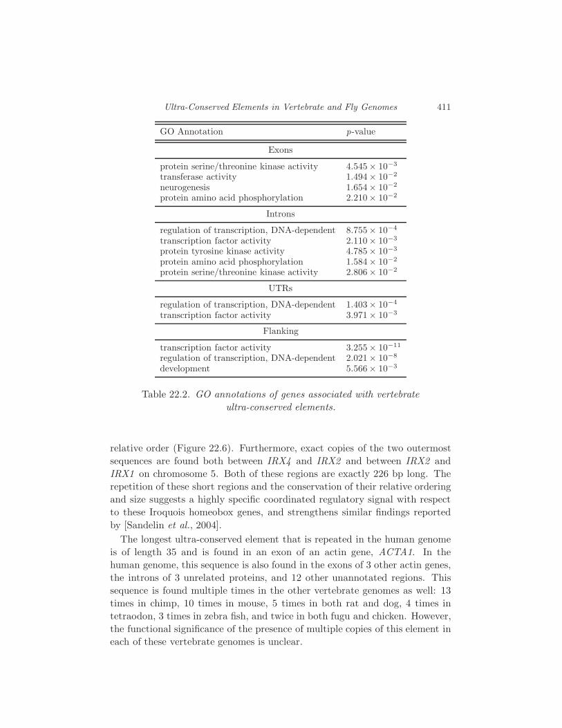
Ultra-Conserved Elements in Vertebrate and Fly Genomes 411
GO Annotation p-value
Exons
protein serine/threonine kinase activity 4.545× 10⁻³
transferase activity 1.494× 10⁻²
neurogenesis 1.654× 10⁻²
protein amino acid phosphorylation 2.210× 10⁻²
Introns
regulation of transcription, DNA-dependent 8.755× 10⁻⁴
transcription factor activity 2.110× 10⁻³
protein tyrosine kinase activity 4.785× 10⁻³
protein amino acid phosphorylation 1.584× 10⁻²
protein serine/threonine kinase activity 2.806× 10⁻²
UTRs
regulation of transcription, DNA-dependent 1.403× 10⁻⁴
transcription factor activity 3.971× 10⁻³
Flanking
transcription factor activity 3.255× 10⁻¹¹
regulation of transcription, DNA-dependent 2.021× 10⁻⁸
development 5.566× 10⁻³
Table 22.2. GO annotations of genes associated with vertebrate
ultra-conserved elements.
relative order (Figure 22.6). Furthermore, exact copies of the two outermost
sequences are found both between IRX4 and IRX2 and between IRX2 and
IRX1 on chromosome 5. Both of these regions are exactly 226 bp long. The
repetition of these short regions and the conservation of their relative ordering
and size suggests a highly specific coordinated regulatory signal with respect
to these Iroquois homeobox genes, and strengthens similar findings reported
by [Sandelin et al., 2004].
The longest ultra-conserved element that is repeated in the human genome
is of length 35 and is found in an exon of an actin gene, ACTA1. In the
human genome, this sequence is also found in the exons of 3 other actin genes,
the introns of 3 unrelated proteins, and 12 other unannotated regions. This
sequence is found multiple times in the other vertebrate genomes as well: 13
times in chimp, 10 times in mouse, 5 times in both rat and dog, 4 times in
tetraodon, 3 times in zebra fish, and twice in both fugu and chicken. However,
the functional significance of the presence of multiple copies of this element in
each of these vertebrate genomes is unclear.

412 M. Drton, N. Eriksson and G. Leung
54102348 TGTAATTACAATCTTACAGAAACCGGGCCGATCTGTATATAAATCTCACCATCCAATTAC54102408 AAGATGTAATAATTTTGCACTCAAGCTGGTAATGAGGTCTAATACTCGTGCATGCGATAA54102468 TCCCCTCTGGATGCTGGCTTGATCAGATGTTGGCTTTGTAATTAGACGGGCAGAAAATCA
54102528 TTATTTCATGTTCAAATAGAAAATGAGGTTGGTGGGAAGTTAATTT
55002049 AAATTAACTTCCCACCAACCTAATTTTTTCCTGAACATGAAATAATGATTTTCTGCCCGT55002109 CTAATTACAAAGCCAACATCTGATCAAGCCAGCATCCAGAGGGGATTATCGCATGCACGA
55002169 GTATTAGACCTCATTACCAGCTTGAGTGCAAAATTATTACATCTTGTAATTGGATGGTGA55002229 GATTTATATACAGATCGGCCCGGTTTCTGTAAGATTGTAATTACA
Fig. 22.6. Sequences found on either side of IRX5. Sequences underlined with a thickline are ultra-conserved with respect to the nine-vertebrate alignment. Sequencesunderlined with a thin line are not ultra-conserved but their reverse complement is.Indices are with respect to chromosome 16.
22.3.2 ENCODE Alignment
Based on the annotations of known human genes provided by the UCSC
Genome Browser, 69.2% of the bases of the ultra-conserved elements of
length at least 20 in the ENCODE alignment overlap intragenic regions (Fig-
ure 22.7(a)). However, longer sequences (at least 50 bp) are heavily biased
towards intronic overlap, accounting for 67.7% of these sequences by base cov-
erage (Figure 22.7(b)).
Introns
Exons
UTRs Unannotated
(a) 524 elements ≥ 20 bp
Introns
ExonsUTRs
Unannotated
(b) 79 elements ≥ 50 bp
Fig. 22.7. Functional base coverage of ultra-conserved elements found in ENCODEregions based on annotations of known human genes.
Values for the gene density and non-exonic conservation level (human-mouse)
are available for the randomly selected ENCODE regions (see Chapter 21 for a
description). For these regions, the amount of base coverage by ultra-conserved
elements is not correlated with gene density (Pearson correlation = -0.0589)
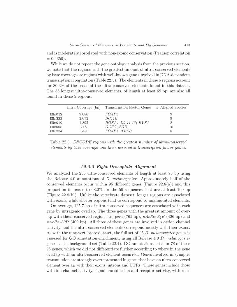
Ultra-Conserved Elements in Vertebrate and Fly Genomes 413
and is moderately correlated with non-exonic conservation (Pearson correlation
= 0.4350).
While we do not repeat the gene ontology analysis from the previous section,
we note that the regions with the greatest amount of ultra-conserved elements
by base coverage are regions with well-known genes involved in DNA-dependent
transcriptional regulation (Table 22.3). The elements in these 5 regions account
for 80.3% of the bases of the ultra-conserved elements found in this dataset.
The 35 longest ultra-conserved elements, of length at least 69 bp, are also all
found in these 5 regions.
Ultra Coverage (bp) Transcription Factor Genes # Aligned Species
ENm012 9,086 FOXP2 9ENr322 2,072 BC11B 9ENm010 1,895 HOXA1-7,9-11,13 ; EVX1 8ENm005 718 GCFC ; SON 10ENr334 549 FOXP4 ; TFEB 8
Table 22.3. ENCODE regions with the greatest number of ultra-conserved
elements by base coverage and their associated transcription factor genes.
22.3.3 Eight-Drosophila Alignment
We analyzed the 255 ultra-conserved elements of length at least 75 bp using
the Release 4.0 annotations of D. melanogaster. Approximately half of the
conserved elements occur within 95 different genes (Figure 22.8(a)) and this
proportion increases to 68.2% for the 59 sequences that are at least 100 bp
(Figure 22.8(b)). Unlike the vertebrate dataset, longer regions are associated
with exons, while shorter regions tend to correspond to unannotated elements.
On average, 125.7 bp of ultra-conserved sequences are associated with each
gene by intragenic overlap. The three genes with the greatest amount of over-
lap with these conserved regions are para (765 bp), nAcRα-34E (426 bp) and
nAcRα-30D (409 bp). All three of these genes are involved in cation channel
activity, and the ultra-conserved elements correspond mostly with their exons.
As with the nine-vertebrate dataset, the full set of 95 D. melanogaster genes is
assessed for GO annotation enrichment, using all Release 4.0 D. melanogaster
genes as the background set (Table 22.4). GO annotations exist for 78 of these
95 genes, which we did not differentiate further according to where in the gene
overlap with an ultra-conserved element occurred. Genes involved in synaptic
transmission are strongly overrepresented in genes that have an ultra-conserved
element overlap with their exons, introns and UTRs. These genes include those
with ion channel activity, signal transduction and receptor activity, with roles
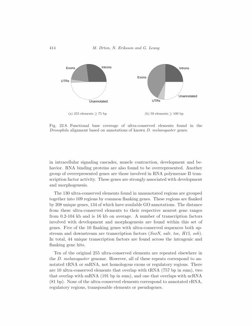
414 M. Drton, N. Eriksson and G. Leung
IntronsExons
UTRs
Unannotated
(a) 255 elements ≥ 75 bp
Introns
Exons
UTRsUnannotated
(b) 59 elements ≥ 100 bp
Fig. 22.8. Functional base coverage of ultra-conserved elements found in theDrosophila alignment based on annotations of known D. melanogaster genes.
in intracellular signaling cascades, muscle contraction, development and be-
havior. RNA binding proteins are also found to be overrepresented. Another
group of overrepresented genes are those involved in RNA polymerase II tran-
scription factor activity. These genes are strongly associated with development
and morphogenesis.
The 130 ultra-conserved elements found in unannotated regions are grouped
together into 109 regions by common flanking genes. These regions are flanked
by 208 unique genes, 134 of which have available GO annotations. The distance
from these ultra-conserved elements to their respective nearest gene ranges
from 0.2-104 kb and is 16 kb on average. A number of transcription factors
involved with development and morphogenesis are found within this set of
genes. Five of the 10 flanking genes with ultra-conserved sequences both up-
stream and downstream are transcription factors (SoxN, salr, toe, H15, sob).
In total, 44 unique transcription factors are found across the intragenic and
flanking gene hits.
Ten of the original 255 ultra-conserved elements are repeated elsewhere in
the D. melanogaster genome. However, all of these repeats correspond to an-
notated tRNA or snRNA, not homologous exons or regulatory regions. There
are 10 ultra-conserved elements that overlap with tRNA (757 bp in sum), two
that overlap with snRNA (191 bp in sum), and one that overlaps with ncRNA
(81 bp). None of the ultra-conserved elements correspond to annotated rRNA,
regulatory regions, transposable elements or pseudogenes.

Ultra-Conserved Elements in Vertebrate and Fly Genomes 415
GO Annotation p-value
Exons, Introns, and UTRs
synaptic transmission 3.290× 10⁻⁹
specification of organ identity 1.044× 10⁻⁶
ventral cord development 3.674× 10⁻⁶
RNA polymerase II transcription factor activity 4.720× 10⁻⁶
muscle contraction 8.714× 10⁻⁶
voltage-gated calcium channel activity 3.548× 10⁻⁵
RNA binding 7.650× 10⁻⁵
synaptic vesicle exocytosis 3.503× 10⁻⁴
leg morphogenesis 3.503× 10⁻⁴
calcium ion transport 6.401× 10⁻⁴
Flanking
regulation of transcription 8.844× 10⁻⁷
neurogenesis 5.339× 10⁻⁶
ectoderm formation 8.285× 10⁻⁶
endoderm formation 2.125× 10⁻⁵
salivary gland morphogenesis 5.870× 10⁻⁵
Notch signaling pathway 1.591× 10⁻⁴
leg joint morphogenesis 1.788× 10⁻⁴
RNA polymerase II transcription factor activity 2.381× 10⁻⁴
salivary gland development 4.403× 10⁻⁴
signal transducer activity 5.308× 10⁻⁴
foregut morphogenesis 8.004× 10⁻⁴
Table 22.4. GO annotations of genes associated with Drosophila
ultra-conserved elements.
22.3.4 Discussion
Previous studies have considered long stretches of perfectly conserved regions
across shorter evolutionary distances [Bejerano et al., 2004], or aligned regions
above some relatively high threshold level of conservation [Boffelli et al., 2004a,
Sandelin et al., 2004, Woolfe et al., 2005]. We, however, focused on ultra-
conserved elements across large evolutionary distances. This approach pre-
cludes our ability to capture all regions containing high levels of conservation,
but allows us to identify regions that appear to be under the most stringent
evolutionary constraints.
As found in previous studies of highly conserved sequences across vertebrate
genomes, non-coding sequences near genes involved in transcriptional regu-
lation are under exceptionally strong evolutionary constraints. Non-coding
regions that are perfectly conserved across all 9 species, such as those found
near the Iroquois homeobox genes on chromosome 16, are excellent candidates

416 M. Drton, N. Eriksson and G. Leung
to be precise regulatory signals. Non-coding sequences near transcription fac-
tors are also found among the Drosophila conserved elements. However, in
the fruit fly dataset, the exonic conservation is more more substantial. Al-
though this conservation is due in part to a much shorter period of evolution,
the exact conservation of exons whose gene products are involved in synaptic
transmission may be fly-specific.
22.4 Probability of Ultra-Conservation
How long of an ultra-conserved element could occur simply by chance? In or-
der to give an answer to this question, let us first assume that the nucleotides
in the different positions in the alignment are mutually independent. Under
this simplifying assumption, we compute the probability of observing an ultra-
conserved element of a given length for the nine-vertebrate and Drosophila-
alignments. While we assume that evolutionary changes to DNA at one po-
sition in the alignment occur independently from changes at all other, and in
particular, neighboring positions, we allow for dependence of the occurrence
of nucleotides in the genomes of different species (at any given position in the
aligned genomes). More precisely, we use a phylogenetic tree model for our
probability calculation.
Before being able to compute a probability, we must build a phyloge-
netic tree and estimate the parameters of the associated model. The tree
for the nine-vertebrate alignment is shown in Figure 22.1. The topology of
this tree is well-known, so we assume it fixed and use paml [Yang, 1997]
to estimate model parameters by maximum likelihood. As input to paml,
we choose the entire alignments with all columns containing a gap removed.
The resulting alignment was 6,300,344 positions long for the vertebrates and
26,216,615 positions long for the Drosophila. Other authors (see Chapter 21
or [Pachter and Sturmfels, 2004a]) have chosen to focus only on synonymous
substitutions in coding regions, since they are likely not selected for or against
and thus give good estimates for neutral substitution rates. However, our in-
dependence model does not depend on the functional structure of the genome,
that is, it sees the columns as i.i.d. samples. Thus, we believe that it is more
appropriate to use all the data available to estimate parameters.
Many phylogenetic tree models exist (cf. Section 4.5) and we concentrate here
on the Jukes-Cantor and HKY models. With the parameter estimates from
paml, we can compute the probability pcons of observing an ultra-conserved
position in the alignment. Recall that the probability pi1...is of seeing the
nucleotide vector (i1, . . . , is) ∈ A, C, G, Ts in a column of the alignment of s
species is given by a polynomial in the entries of the transition matrices Pe(t),
which are obtained as Pe(t) = exp(Qte) where te is the length of the edge e
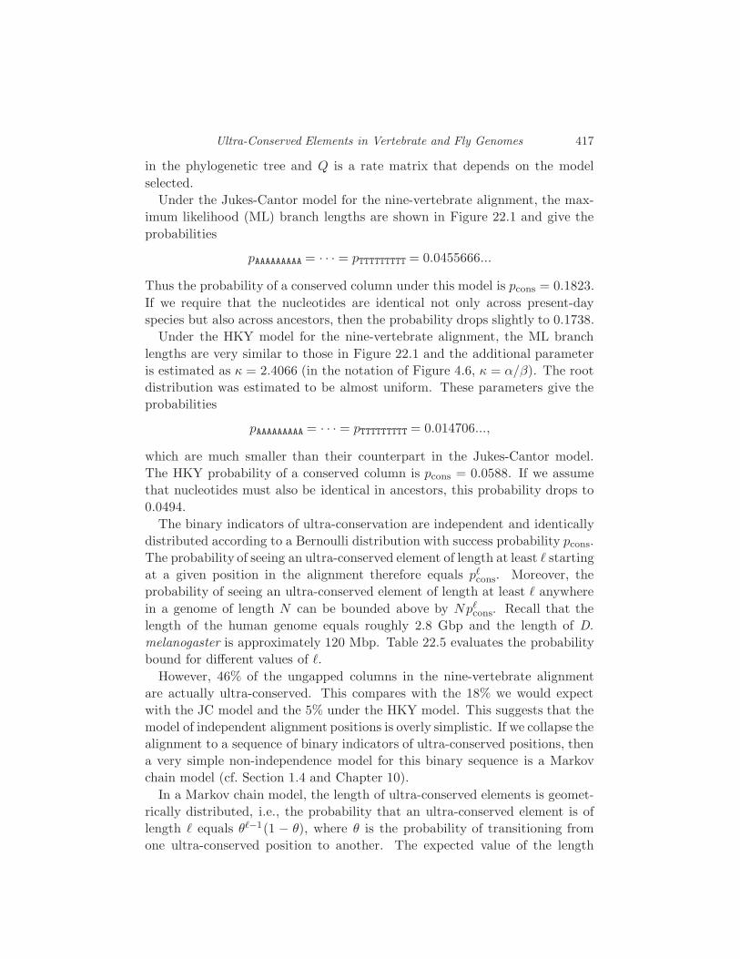
Ultra-Conserved Elements in Vertebrate and Fly Genomes 417
in the phylogenetic tree and Q is a rate matrix that depends on the model
selected.
Under the Jukes-Cantor model for the nine-vertebrate alignment, the max-
imum likelihood (ML) branch lengths are shown in Figure 22.1 and give the
probabilities
pAAAAAAAAA = · · · = pTTTTTTTTT = 0.0455666...
Thus the probability of a conserved column under this model is pcons = 0.1823.
If we require that the nucleotides are identical not only across present-day
species but also across ancestors, then the probability drops slightly to 0.1738.
Under the HKY model for the nine-vertebrate alignment, the ML branch
lengths are very similar to those in Figure 22.1 and the additional parameter
is estimated as κ = 2.4066 (in the notation of Figure 4.6, κ = α/β). The root
distribution was estimated to be almost uniform. These parameters give the
probabilities
pAAAAAAAAA = · · · = pTTTTTTTTT = 0.014706...,
which are much smaller than their counterpart in the Jukes-Cantor model.
The HKY probability of a conserved column is pcons = 0.0588. If we assume
that nucleotides must also be identical in ancestors, this probability drops to
0.0494.
The binary indicators of ultra-conservation are independent and identically
distributed according to a Bernoulli distribution with success probability pcons.
The probability of seeing an ultra-conserved element of length at least ℓ starting
at a given position in the alignment therefore equals pℓcons. Moreover, the
probability of seeing an ultra-conserved element of length at least ℓ anywhere
in a genome of length N can be bounded above by Npℓcons. Recall that the
length of the human genome equals roughly 2.8 Gbp and the length of D.
melanogaster is approximately 120 Mbp. Table 22.5 evaluates the probability
bound for different values of ℓ.
However, 46% of the ungapped columns in the nine-vertebrate alignment
are actually ultra-conserved. This compares with the 18% we would expect
with the JC model and the 5% under the HKY model. This suggests that the
model of independent alignment positions is overly simplistic. If we collapse the
alignment to a sequence of binary indicators of ultra-conserved positions, then
a very simple non-independence model for this binary sequence is a Markov
chain model (cf. Section 1.4 and Chapter 10).
In a Markov chain model, the length of ultra-conserved elements is geomet-
rically distributed, i.e., the probability that an ultra-conserved element is of
length ℓ equals θℓ−1(1 − θ), where θ is the probability of transitioning from
one ultra-conserved position to another. The expected value of the length
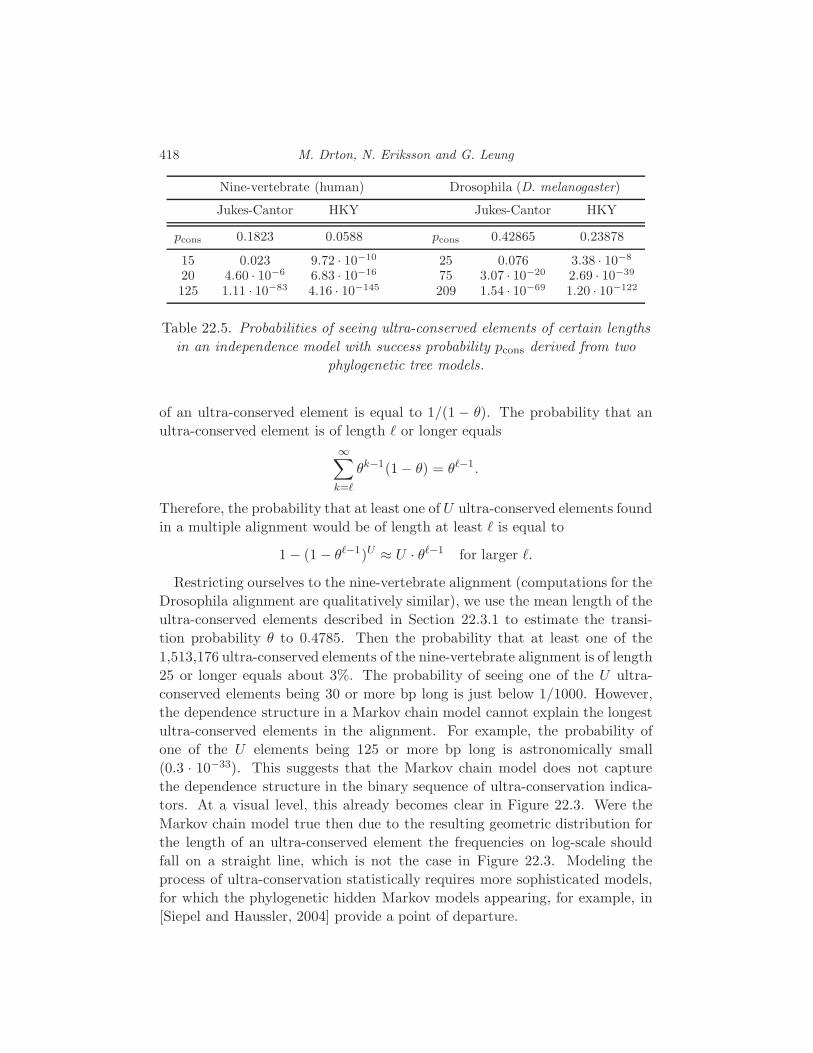
418 M. Drton, N. Eriksson and G. Leung
Nine-vertebrate (human) Drosophila (D. melanogaster)
Jukes-Cantor HKY Jukes-Cantor HKY
pcons 0.1823 0.0588 pcons 0.42865 0.23878
15 0.023 9.72 · 10−10 25 0.076 3.38 · 10−8
20 4.60 · 10−6 6.83 · 10−16 75 3.07 · 10−20 2.69 · 10−39
125 1.11 · 10−83 4.16 · 10−145 209 1.54 · 10−69 1.20 · 10−122
Table 22.5. Probabilities of seeing ultra-conserved elements of certain lengths
in an independence model with success probability pcons derived from two
phylogenetic tree models.
of an ultra-conserved element is equal to 1/(1 − θ). The probability that an
ultra-conserved element is of length ℓ or longer equals
∞∑
k=ℓ
θk−1(1− θ) = θℓ−1.
Therefore, the probability that at least one of U ultra-conserved elements found
in a multiple alignment would be of length at least ℓ is equal to
1 − (1 − θℓ−1)U ≈ U · θℓ−1 for larger ℓ.
Restricting ourselves to the nine-vertebrate alignment (computations for the
Drosophila alignment are qualitatively similar), we use the mean length of the
ultra-conserved elements described in Section 22.3.1 to estimate the transi-
tion probability θ to 0.4785. Then the probability that at least one of the
1,513,176 ultra-conserved elements of the nine-vertebrate alignment is of length
25 or longer equals about 3%. The probability of seeing one of the U ultra-
conserved elements being 30 or more bp long is just below 1/1000. However,
the dependence structure in a Markov chain model cannot explain the longest
ultra-conserved elements in the alignment. For example, the probability of
one of the U elements being 125 or more bp long is astronomically small
(0.3 · 10−33). This suggests that the Markov chain model does not capture
the dependence structure in the binary sequence of ultra-conservation indica-
tors. At a visual level, this already becomes clear in Figure 22.3. Were the
Markov chain model true then due to the resulting geometric distribution for
the length of an ultra-conserved element the frequencies on log-scale should
fall on a straight line, which is not the case in Figure 22.3. Modeling the
process of ultra-conservation statistically requires more sophisticated models,
for which the phylogenetic hidden Markov models appearing, for example, in
[Siepel and Haussler, 2004] provide a point of departure.

Bibliography
[Abril et al., 2005] JF Abril, R Castelo, and R Guigo. Comparison of splice sites inmammals and chicken. Genome Research, 15:111–119, 2005. pages 152
[Adkins et al., 2001] RM Adkins, EL Gelke, D Rowe, and RL Honeycutt. MolecularPhylogeny and Divergence Time Estimates for Major Rodent Groups: Evidencefrom Multiple Genes. Mol Biol Evol, 18(5):777–791, 2001. pages 397
[Agresti, 1990] A Agresti. Categorical data analysis. Wiley Series in Probability andMathematical Statistics: Applied Probability and Statistics. John Wiley & SonsInc., New York, 1990. A Wiley-Interscience Publication. pages 14
[Aji and McEliece, 2000] SM Aji and RJ McEliece. The generalized distributive law.IEEE Trans. Inform. Theory, 46(2):325–343, 2000. pages 44
[Alefeld and Herzberger, 1983] G Alefeld and J Herzberger. An introduction to intervalcomputations. Academic press, New York, 1983. pages 377
[Alexandersson et al., 2003] M Alexandersson, S Cawley, and L Pachter. Slam: cross-species gene finding and alignment with a generalized pair hidden markov model.Genome Res, 13(3):496–502, 2003. pages 154
[Allman and Rhodes, 2003] ES Allman and JA Rhodes. Phylogenetic invariants forthe general Markov model of sequence mutation. Math. Biosci., 186(2):113–144,2003. pages 161, 361
[Allman and Rhodes, 2004a] ES Allman and JA Rhodes. Phylogenetic ideals and va-rieties for the general markov model, 2004. pages 313, 325, 328, 361, 364
[Allman and Rhodes, 2004b] ES Allman and JA Rhodes. Quartets and parameter re-covery for the general Markov model of sequence mutation. AMRX Appl. Math.Res. Express, 2004(4):107–131, 2004. pages 108, 361, 364
[Altschul et al., 1990] SF Altschul, W Gish, W Miller, EW Myers, and DJ Lipman.Basic local alignment search tool. J Molecular Biology, 215:403–410, 1990. pages85
[Andrews, 1963] G Andrews. A lower bound on the volume of strictly convex bodieswith many boundary points. Trans. Amer. Math. Soc., 106:270–279, 1963. pages181
[Apostol, 1976] TM Apostol. Introduction to analytic number theory. Springer-Verlag,New York, 1976. Undergraduate Texts in Mathematics. pages 228
[Ardila, 2004] F Ardila. A tropical morphism related to the hyperplane arrangement ofthe complete bipartite graph. Discrete and Computational Geometry, to appear,2004. pages 123
[Aris-Brosou, 2003] S Aris-Brosou. How bayes tests of molecular phylogenies comparewith frequentist approaches. Bioinformatics, 19:618–624, 2003. pages 388
[Ashburner et al., 2000] M Ashburner, CA Ball, JA Blake, D Botstein, H Butler,JM Cherry, K Dolinski, SS Dwight, JT Eppig, MA Harris, DP Hill, L Issel-Tarver,A Kasarskis, S Lewis, JC Matese, JE Richardson, M Ringwald, GM Rubin, andG Sherlock. Gene ontology: tool for the unification of biology. the gene ontologyconsortium. Nature Genetics, 25:25–29, 2000. pages 410
[Bandelt and Dress, 1992] HJ Bandelt and AWM Dress. A canonical decompositiontheory for metrics on a finite set. Advances in Mathematics, 92:47–105, 1992.pages 332, 336
[Bandelt et al., 1995] HJ Bandelt, P Forster, BC Sykes, and MB Richards. Mitochon-drial portraits of human population using median networks. Genetics, 141:743–753, 1995. pages 332
[Basu et al., 2003] S Basu, R Pollack, and MF Roy. Algorithms in real algebraic geom-etry, volume 10 of Algorithms and Computation in Mathematics. Springer-Verlag,Berlin, 2003. pages 101
419
[Beerenwinkel et al., 2004] N Beerenwinkel, J Rahnenfuhrer, M Daumer, D Hoffmann,R Kaiser, J Selbig, and T Lengauer. Learning multiple evolutionary pathwaysfrom cross-sectional data. In Proc. 8th Ann. Int. Conf. on Res. in Comput. Biol.(RECOMB ’04), 27–31 March 2004, San Diego, CA, pages 36–44, 2004. to appearin J. Comp. Biol. pages 284, 287, 295
[Beerenwinkel et al., 2005a] N Beerenwinkel, M Daumer, T Sing, J Rahnenfuhrer,T Lengauer, J Selbig, D Hoffmann, and R Kaiser. Estimating HIV evolution-ary pathways and the genetic barrier to drug resistance. J. Infect. Dis., 2005. toappear. pages 284
[Beerenwinkel et al., 2005b] N Beerenwinkel, J Rahnenfuhrer, R Kaiser, D Hoffmann,J Selbig, and T Lengauer. Mtreemix: a software package for learning and usingmixture models of mutagenetic trees. Bioinformatics, 2005. to appear. pages285
[Bejerano et al., 2004] G Bejerano, M Pheasant, I Makunin, S Stephen, WJ Kent,JS Mattick, and D Haussler. Ultraconserved elements in the human genome.Science, 304:1321–1325, 2004. pages 410, 415
[Besag, 1986] J Besag. On the statistical analysis of dirty pictures. Journal of theRoyal Statistical Society, B 48 No. 3:259–302, 1986. pages 280, 281
[Bickel, 1971] PJ Bickel. Mathematical Statistics, Part I. Holden-Day Inc., San Fran-cisco, Calif., 1971. Basic ideas and selected topics, Holden-Day Series in Proba-bility and Statistics. pages 6, 8
[Boffelli et al., 2003] Dario Boffelli, Jon McAuliffe, Dmitriy Ovcharenko, Keith DLewis, Ivan Ovcharenko, Lior Pachter, and Edward M Rubin. Phylogenetic shad-owing of primate sequences to find functional regions of the human genome. Sci-ence, 299(5611):1391–4, 2003. pages 138, 164
[Boffelli et al., 2004a] D. Boffelli, M.A. Nobrega, and E.M. Rubin. Comparative ge-nomics at the vertebrate extremes. Nature Reviews Genetics, 5:456–465, 2004.pages 410, 415
[Boffelli et al., 2004b] D Boffelli, CV Weer, L Weng, KD Lewis, MI Shoukry, L Pachter,DN Keys, and EM Rubin. Intraspecies sequence comparisons for annotatinggenomes. Genome Research, 14:2406–2411, 2004. pages 138
[Bosma et al., 1997] Wieb Bosma, John Cannon, and Catherine Playoust. TheMAGMA algebra system I: the user language. J. Symb. Comput., 24(3-4):235–265, 1997. pages 81
[Bourque et al., 2004] Guillaume Bourque, Pavel A Pevzner, and Glenn Tesler. Recon-structing the genomic architecture of ancestral mammals: lessons from human,mouse, and rat genomes. Genome Res, 14(4):507–16, 2004. pages 139
[Bray and Pachter, 2004] N Bray and L Pachter. Mavid: constrained ancestral align-ment of multiple sequences. Genome Res, 14(4):693–9, 2004. pages 86, 393,403
[Brown et al., 1982] WM Brown, EM Prager, A Wang, and AC Wilson. MitochondrialDNA sequences of primates, tempo and mode of evolution. Journal of MolecularEvolution, 18:225–239, 1982. pages 386
[Brown, 2002] TA Brown. Genomes 2. John Wiley & Son, Inc., 2002. pages 2, 138[Brudno et al., 2003] M. Brudno, S. Malde, A. Poliakov, C. Do, O. Courone,
I. Dubchak, and S. Batzoglou. Global alignment: finding rearrangements duringalignment. Special issue on the Proceedings of the ISMB 2003, Bioinformatics,19:54i–64i, 2003. pages 393, 404
[Bryant and Moulton, 2004] D Bryant and V Moulton. Neighbornet: An agglomerativealgorithm for the construction of planar phylogenetic networks. Molecular BiologyAnd Evolution, 21:255–265, 2004. pages 332
[Buchberger, 1965] B Buchberger. An algorithm for finding a basis for the residue
420

class ring of a zero-dimensional polynomial ideal (in German). PhD thesis, Univ.Innsbruck, Dept. of Math., Innsbruck, Austria, 1965. pages 98
[Bulmer, 1991] D Bulmer. Use of the method of generalized least squares in reconstruct-ing phylogenies from sequence data. Molecular Biology and Evolution, 8(6):868–883, 1991. pages 335
[Burge and Karlin, 1997] C Burge and S Karlin. Prediction of complete gene structuresin human genomic DNA. Journal of Molecular Biology, 268(1):78–94, 1997. pages154
[Campbell et al., 1999] A Campbell, J Mrazek, and S Karlin. Genome signature com-parisons among prokaryote, plasmid and mitochondrial DNA. Proceedings of theNational Academy of Sciences USA, 96(16):9184–9189, 1999. pages 136, 137
[Casanellas et al., 2004] M. Casanellas, L.D. Garcia, and S. Sullivant. Small phy-logenetic trees. http://www.math.tamu.edu/∼lgp/small-trees/small-trees.html,2004. pages 308
[Catalisano et al., 2002] M. V. Catalisano, A. V. Geramita, and A. Gimigliano. Ranksof tensors, secant varieties of Segre varieties and fat points. Linear Algebra Appl.,355:263–285, 2002. pages 295
[Catanese et al., 2004] Fabrizio Catanese, Serkan Hosten, Amit Khetan, and BerndSturmfels. The maximum likelihood degree. to appear in the American Journalof Mathematics, 2004. pages 11, 112
[Cavalli-Sforza and Edwards, 1967] L. Cavalli-Sforza and A. Edwards. Phylogeneticanalysis models and estimation procedures. Evolution, 32:550–570, 1967. pages335
[Cavender and Felsenstein, 1987] J. Cavender and J. Felsenstein. Invariants of phylo-genies in a simple case with discrete states. Journal of Classification, 4:57–71,1987. pages 361
[Chargaff, 1950] E Chargaff. Chemical specificity of nucleic acids and mechanism forthe enzymatic degradation. Experientia, 6:201–209, 1950. pages 135
[Chazelle, 1991] B Chazelle. An optimal convex hull algorithm and new results oncuttings. In Proc. 32nd IEEE Symp. on Foundations of Computer Science, pages29–38, 1991. pages 183
[Chazelle, 1993] B Chazelle. An optimal convex hull algorithm in any fixed dimension.Discrete Computational Geometry, 10:377–409, 1993. pages 183
[Cohen and Rothblum, 1993] Joel E. Cohen and Uriel G. Rothblum. Nonnegativeranks, decompositions, and factorizations of nonnegative matrices. Linear Al-gebra Appl., 190:149–168, 1993. pages 123
[Cohen, 2004] Joel E Cohen. Mathematics is biology’s next microscope, only better;biology is mathematics’ next physics, only better. PLoS Biol, 2(12):e439, 2004.pages 2
[Consortium, 2004] ENCODE Project Consortium. The encode (encyclopedia of dnaelements) project. Science, 306(5696):636–40, 2004. pages 149, 393
[Cox et al., 1997] David Cox, John Little, and Donal O’Shea. Ideals, varieties, andalgorithms. Undergraduate Texts in Mathematics. Springer-Verlag, New York,second edition, 1997. An introduction to computational algebraic geometry andcommutative algebra. pages 2, 93, 97, 101, 103, 244
[Craciun and Feinberg, 2004] G Craciun and M Feinberg. Multiple equilibria in com-plex chemical reaction networks: I. the injectivity property. SIAM Journal ofApplied Mathematics, 2004. pages 100
[Cuyt et al., 2001] A Cuyt, B Verdonk, S Becuwe, and P Kuterna. A remarkable exam-ple of catastrophic cancellation unraveled. Computing, 66:309–320, 2001. pages374
[Darwin, 1859] C Darwin. On the origin of species by means of natural selection, or
421

the preservation of favoured races in the struggle for life. John Murray, London,1859. pages 71, 147
[De Concini et al., 1982] Corrado De Concini, David Eisenbud, and Claudio Procesi.Hodge algebras, volume 91 of Asterisque. Societe Mathematique de France, Paris,1982. With a French summary. pages 107
[Demmel, 1997] James W. Demmel. Applied numerical linear algebra. Society for In-dustrial and Applied Mathematics (SIAM), Philadelphia, PA, 1997. pages 364
[Desper et al., 1999] R. Desper, F. Jiang, O.-P. Kallioniemi, H. Moch, C.H. Papadim-itriou, and A.A. Schaffer. Inferring tree models for oncogenesis from comparativegenome hybridization data. J. Comp. Biol., 6(1):37–51, 1999. pages 284
[Develin and Sturmfels, 2004] Mike Develin and Bernd Sturmfels. Tropical convexity.Doc. Math., 9:1–27 (electronic), 2004. pages 121, 123
[Develin et al., 2003] M Develin, F Santos, and B Sturmfels. On the tropical rank of amatrix. MSRI Proceedings, to appear, 2003. pages 121, 123
[Dewey et al., 2004] Colin Dewey, Jia Qian Wu, Simon Cawley, Marina Alexandersson,Richard Gibbs, and Lior Pachter. Accurate identification of novel human genesthrough simultaneous gene prediction in human, mouse, and rat. Genome Res,14(4):661–4, 2004. pages 137
[Dewey, 2005] Colin Dewey. Mercator: software for multi-ple whole-genome orthology map construction. Available athttp://hanuman.math.berkeley.edu/ cdewey/mercator/, 2005. pages 393,403
[Deza and Laurent, 1997] Michel Marie Deza and Monique Laurent. Geometry of cutsand metrics, volume 15 of Algorithms and Combinatorics. Springer-Verlag, Berlin,1997. pages 71
[Douzery E. J. P. and D., 2003] Stanhope M. J. Douzery E. J. P., Delsuc F. and Hu-chon D. Local molecular clocks in three nuclear genes: divergence ages of rodentsand other mammals, and incompatibility between fossil calibrations. MolecularBiology and Evolution, 57:201–213, 2003. pages 402
[Dress and Huson, 2004] A. Dress and Daniel Huson. Constructing splits graphs.IEEE/ACM Transactions in Computational Biology and Bioinformatics, 2004.pages 333
[Dress and Terhalle, 1998] Andreas Dress and Werner Terhalle. The tree of life andother affine buildings. In Proceedings of the International Congress of Mathemati-cians, number Extra Vol. III in Vol. III (Berlin, 1998), pages 565–574 (electronic),1998. pages 125
[Dress et al., 2002] A. Dress, J. H. Koolen, and V. Moulton. On line arrangements inthe hyperbolic plane. European J. Combin., 23(5):549–557, 2002. pages 107
[Durbin et al., 1998] R Durbin, S Eddy, A Korgh, and G Mitchison. Biological Se-quence Analysis: Probabilistic Models of Proteins and Nucleic Acids. CambridgeUniversity Press, 1998. pages 2, 3, 4, 25, 28, 31, 150, 259
[Eichler and Sankoff, 2003] EE Eichler and D. Sankoff. Structural dynamics of eukary-otic chromosome evolution. Science, 301:793–797, 2003. pages 138
[Evans and Speed, 1993] S Evans and T Speed. Invariants of some probability modelsused in phylogenetic inference. The Annals of Statistics, 21:355–377, 1993. pages161, 303, 312, 316
[Farris, 1972] J.S. Farris. Estimating phylogenetic trees from distance matrices. Amer-ican Naturalist, 106:645–668, 1972. pages 335
[Felsenstein, 1978] J. Felsenstein. Cases in which parsimony or compatibility methodswill be positively misleading. Syst. Zool., 22:240–249, 1978. pages 400
[Felsenstein, 1981] J Felsenstein. Evolutionary trees from DNA sequences: a maximumlikelihood approach. Journal of Molecular Evolution, 17:368–376, 1981. pages
422

335, 380[Felsenstein, 2003] J Felsenstein. Inferring Phylogenies. Sinauer Associates, Inc., 2003.
pages vii, 71, 156, 161, 336[Felsenstein, 2004] J Felsenstein. PHYLIP (Phylogeny Inference Package) version 3.6.
Distributed by the author, Department of Genome Sciences, University of Wash-ington, Seattle, 2004. pages 88, 389, 390
[Fernandez-Baca et al., 2002] D Fernandez-Baca, T Seppalainen, and G Slutzki.Bounds for parametric sequence comparison. Discrete Applied Mathematics,118:181–198, 2002. pages 214, 218, 219, 220
[Fitch and Smith, 1983] Walter M. Fitch and Temple F. Smith. Optimal SequenceAlignments. PNAS, 80(5):1382–1386, 1983. pages 213
[Fleischmann et al., 1995] RD Fleischmann, MD Adams, O White, RA Clayton,EF Kirkness, AR Kerlavage, CJ Bult, JF Tomb, BA Dougherty, and JM Merricket al. Whole-genome random sequencing and assembly of haemophilus influenzaRd. Science, 269(5223):496–512, 1995. pages 133
[Floyd, 1962] RW Floyd. Algorithm 97: shortest path. Communications of ACM,5(6):345, 1962. pages 48
[Forney, 1973] G.D. Forney. The viterbi algorithm. Proc. of the IEEE, 61(3):268–278,1973. pages 232
[Frieze et al., 1998] A. Frieze, R. Kannan, and S. Vempala. Fast Monte Carlo algo-rithms for low rank approximation. In 39th Symposium on Foundations of Com-puting, pages 370–378, 1998. pages 366
[Fukuda, 2004] Komei Fukuda. From the zonotope construction to the Minkowski ad-dition of convex polytopes. J. Symbolic Comput., 38(4):1261–1272, 2004. pages194
[Galtier and Gouy, 1998] N. Galtier and M. Gouy. Inferring pattern and process: max-imum likelihood implementation of a non-homogeneous model of dna sequenceevolution for phylogenetic analysis. Molecular Biology and Evolution, 154(4):871–879, 1998. pages 400, 401
[Garcia et al., 2004] L. D. Garcia, M. Stillman, and B. Sturmfels. Algebraic geometry ofBayesian networks. J. Symbolic Comput., 2004. Special Issue Methodes Effectivesen Geometrie Algebrique (MEGA). pages 42, 108, 289, 364
[Garcia, 2004] L. D. Garcia. Algebraic statistics in model selection. In M. Chickeringand J. Halpern, editors, Proceedings of the 20th Conference on Uncertainty inArtificial Intelligence, pages 177–184. AUAI Press, Arlington, VA, 2004. pages295
[Gatermann and Wolfrum, 2005] K Gatermann and M Wolfrum. Bernstein’s secondtheorem and viro’s method for sparse polynomial systems in chemistry. Advancesin Applied Mathematics, 34(2):252–294, 2005. pages 100
[Gawrilow and Joswig, 2000] Ewgenij Gawrilow and Michael Joswig. polymake: aframework for analyzing convex polytopes. In Gil Kalai and Gunter M. Ziegler,editors, Polytopes — Combinatorics and Computation, pages 43–74. Birkhauser,2000. pages 84
[Gawrilow and Joswig, 2001] Ewgenij Gawrilow and Michael Joswig. polymake: anapproach to modular software design in computational geometry. In Proceedings ofthe 17th Annual Symposium on Computational Geometry, pages 222–231. ACM,2001. June 3-5, 2001, Medford, MA. pages 84
[Geiger et al., 2001] Dan Geiger, David Heckerman, Henry King, and ChristopherMeek. Stratified exponential families: graphical models and model selection.Ann. Statist., 29(2):505–529, 2001. pages 297
[Geiger et al., 2002] D. Geiger, C. Meek, and B. Sturmfels. On the toric algebra ofgraphical models. Annals of Statistics, 2002. pages 272
423

[Geiger et al., 2005] D. Geiger, C. Meek, and B. Sturmfels. On the toric algebra ofgraphical models. Ann. Statist., to appear, 2005. pages 40, 289
[Geman and Geman, 1984] S. Geman and D. Geman. Stochastic relaxation, gibbs dis-tributions and the bayesian restoration of images. IEEE Transactions on PatternAnalysis and Machine Intelligence, PAMI-6, pages 721–741, 1984. pages 280
[Gentleman et al., 2004] Robert C Gentleman, Vincent J. Carey, Douglas M. Bates,Ben Bolstad, Marcel Dettling, Sandrine Dudoit, Byron Ellis, Laurent Gautier,Yongchao Ge, Jeff Gentry, Kurt Hornik, Torsten Hothorn, Wolfgang Huber, Ste-fano Iacus, Rafael Irizarry, Friedrich Leisch Cheng Li, Martin Maechler, An-thony J. Rossini, Gunther Sawitzki, Colin Smith, Gordon Smyth, Luke Tierney,Jean Y. H. Yang, and Jianhua Zhang. Bioconductor: Open software developmentfor computational biology and bioinformatics. Genome Biology, 5:R80, 2004.pages 84
[Gentles and Karlin, 2001] AJ Gentles and S Karlin. Genome-scale compositional com-parisons in eukaryotes. Genome Research, 4:540–546, 2001. pages 136
[Gibbs et al., 2004] Richard A Gibbs, George M Weinstock, Michael L Metzker,Donna M Muzny, Erica J Sodergren, Steven Scherer, Graham Scott, David Stef-fen, Kim C Worley, Paula E Burch, Geoffrey Okwuonu, Sandra Hines, Lora Lewis,Christine DeRamo, Oliver Delgado, Shannon Dugan-Rocha, George Miner, Mar-garet Morgan, Alicia Hawes, Rachel Gill, Robert A Holt, Mark D Adams, Peter GAmanatides, Holly Baden-Tillson, Mary Barnstead, Soo Chin, Cheryl A Evans,Steve Ferriera, Carl Fosler, Anna Glodek, Zhiping Gu, Don Jennings, Cheryl LKraft, Trixie Nguyen, Cynthia M Pfannkoch, Cynthia Sitter, Granger G Sutton,J Craig Venter, Trevor Woodage, Douglas Smith, Hong-Mei Lee, Erik Gustafson,Patrick Cahill, Arnold Kana, Lynn Doucette-Stamm, Keith Weinstock, Kim Fech-tel, Robert B Weiss, Diane M Dunn, Eric D Green, Robert W Blakesley, Ger-ard G Bouffard, Pieter J De Jong, Kazutoyo Osoegawa, Baoli Zhu, Marco Marra,Jacqueline Schein, Ian Bosdet, Chris Fjell, Steven Jones, Martin Krzywinski, Car-rie Mathewson, Asim Siddiqui, Natasja Wye, John McPherson, Shaying Zhao,Claire M Fraser, Jyoti Shetty, Sofiya Shatsman, Keita Geer, Yixin Chen, SofyiaAbramzon, William C Nierman, Paul H Havlak, Rui Chen, K James Durbin,Amy Egan, Yanru Ren, Xing-Zhi Song, Bingshan Li, Yue Liu, Xiang Qin, Si-mon Cawley, A J Cooney, Lisa M D’Souza, Kirt Martin, Jia Qian Wu, Manuel LGonzalez-Garay, Andrew R Jackson, Kenneth J Kalafus, Michael P McLeod,Aleksandar Milosavljevic, Davinder Virk, Andrei Volkov, David A Wheeler,Zhengdong Zhang, Jeffrey A Bailey, Evan E Eichler, Eray Tuzun, Ewan Bir-ney, Emmanuel Mongin, Abel Ureta-Vidal, Cara Woodwark, Evgeny Zdobnov,Peer Bork, Mikita Suyama, David Torrents, Marina Alexandersson, Barbara JTrask, Janet M Young, Hui Huang, Huajun Wang, Heming Xing, Sue Daniels,Darryl Gietzen, Jeanette Schmidt, Kristian Stevens, Ursula Vitt, Jim Wingrove,Francisco Camara, M Mar Alba, Josep F Abril, Roderic Guigo, Arian Smit,Inna Dubchak, Edward M Rubin, Olivier Couronne, Alexander Poliakov, Nor-bert Hubner, Detlev Ganten, Claudia Goesele, Oliver Hummel, Thomas Kreitler,Young-Ae Lee, Jan Monti, Herbert Schulz, Heike Zimdahl, Heinz Himmelbauer,Hans Lehrach, Howard J Jacob, Susan Bromberg, Jo Gullings-Handley, Michael IJensen-Seaman, Anne E Kwitek, Jozef Lazar, Dean Pasko, Peter J Tonellato,Simon Twigger, Chris P Ponting, Jose M Duarte, Stephen Rice, Leo Goodstadt,Scott A Beatson, Richard D Emes, Eitan E Winter, Caleb Webber, Petra Brandt,Gerald Nyakatura, Margaret Adetobi, Francesca Chiaromonte, Laura Elnitski,Pallavi Eswara, Ross C Hardison, Minmei Hou, Diana Kolbe, Kateryna Makova,Webb Miller, Anton Nekrutenko, Cathy Riemer, Scott Schwartz, James Taylor,Shan Yang, Yi Zhang, Klaus Lindpaintner, T Dan Andrews, Mario Caccamo,
424

Michele Clamp, Laura Clarke, Valerie Curwen, Richard Durbin, Eduardo Eyras,Stephen M Searle, Gregory M Cooper, Serafim Batzoglou, Michael Brudno, ArendSidow, Eric A Stone, Bret A Payseur, Guillaume Bourque, Carlos Lopez-Otin,Xose S Puente, Kushal Chakrabarti, Sourav Chatterji, Colin Dewey, Lior Pachter,Nicolas Bray, Von Bing Yap, Anat Caspi, Glenn Tesler, Pavel A Pevzner, DavidHaussler, Krishna M Roskin, Robert Baertsch, Hiram Clawson, Terrence S Furey,Angie S Hinrichs, Donna Karolchik, William J Kent, Kate R Rosenbloom, HeatherTrumbower, Matt Weirauch, David N Cooper, Peter D Stenson, Bin Ma, MichaelBrent, Manimozhiyan Arumugam, David Shteynberg, Richard R Copley, Mar-tin S Taylor, Harold Riethman, Uma Mudunuri, Jane Peterson, Mark Guyer,Adam Felsenfeld, Susan Old, Stephen Mockrin, and Francis Collins. Genome se-quence of the brown norway rat yields insights into mammalian evolution. Nature,428(6982):493–521, 2004. pages 138, 397
[Grayson and Stillman, 2002] Daniel R. Grayson and Michael E. Stillman. Macaulay2, a software system for research in algebraic geometry. Available athttp://www.math.uiuc.edu/Macaulay2/, 2002. pages 80, 244, 318, 321
[Greuel and Pfister, 2002] GM Greuel and G Pfister. A Singular Introduction to Com-mutative Algebra. Springer-Verlag, Berlin and Heidelberg, 2002. pages 84
[Greuel et al., 2003] GM Greuel, G. Pfister, and H. Schoenemann. Singular,a computer algebra system for polynomial computations. Available athttp://www.singular.uni-kl.de/, 2003. pages 244
[Griffiths and Marjoram, 1996] R. C. Griffiths and P. Marjoram. Ancestral inferencefrom samples of dna sequences with recombination. Journal of ComputationalBiology, 3(4):479–502, 1996. pages 332
[Grotschel et al., 1993] Martin Grotschel, Laszlo Lovasz, and Alexander Schrijver. Ge-ometric Algorithms and Combinatorial Optimization, volume 2 of Algorithms andCombinatorics. Springer-Verlag, 1993. pages 182, 192
[Grunbaum, 2003] Branko Grunbaum. Convex polytopes, volume 221 of Graduate Textsin Mathematics. Springer-Verlag, New York, second edition, 2003. Prepared andwith a preface by Volker Kaibel, Victor Klee and Gunter M. Ziegler. pages 63
[Guigo et al., 2004] R Guigo, E Birbey, M Brent, E Dermitzakis, L Pachter, H RoestCrollius, V Solovyev, and MQ Zhang. Needed for completion of the humangenome: hypothesis driven experiments and biologically realistic mathematicalmodels. arXiv q-bio.GN/0410008, 2004. pages 138
[Gusfield et al., 1994] D Gusfield, K Balasubramanian, and D Naor. Parametric opti-mization of sequence alignment. Algorithmica, 12:312–326, 1994. pages 58, 201,216, 218
[Gusfield, 1997] D Gusfield. Algorithms on Strings, Trees, and Sequences. CambridgeUniversity Press, 1997. pages 52, 58, 202, 213
[Hacijan, 1979] L. G. Hacijan. A polynomial algorithm in linear programming. Dokl.Akad. Nauk SSSR, 244(5):1093–1096, 1979. pages 192
[Hallgrimsdottir and Sturmfels, 2004] I Hallgrimsdottir and B Sturmfels. Resultantsin genetic linkage analysis. Journal of Symbolic Computation, to appear, 2004.pages 134
[Hammer et al., 1995] R Hammer, M Hocks, U Kulisch, and D Ratz. C++ toolboxfor verified computing: basic numerical problems. Springer-Verlag, Berlin, 1995.pages 379, 380
[Hannenhalli and Pevzner, 1999] Sridhar Hannenhalli and Pavel A. Pevzner. Trans-forming cabbage into turnip: polynomial algorithm for sorting signed permuta-tions by reversals. Journal of the ACM, 46(1):1—-27, 1999. pages 138
[Hansen and Sengupta, 1981] E Hansen and S Sengupta. Bounding solutions of systemsof equations using interval analysis. BIT, 21:203–211, 1981. pages 379
425

[Hansen, 1980] E Hansen. Global optimization using interval analysis - the multi-dimensional case. Numerische Mathematik, 34:247–270, 1980. pages 374
[Hansen, 1992] E Hansen. Global optimization using interval analysis. Marcel Dekker,New York, 1992. pages 379, 384
[Hendy and Penny, 1989] M. Hendy and D. Penny. A framework for the quantitativestudy of evolutionary trees. Systematic Zoology, 38(4), 1989. pages 342, 345, 400
[Hendy and Penny, 1993] MD Hendy and D Penny. Spectral analysis of phylogeneticdata. Journal of Classification, 10:5–24, 1993. pages 161
[Hibi, 1987] T. Hibi. Distributive lattices, affine semigroup rings and algebras withstraightening laws. Advanced Studies in Pure Mathematics, 11:93–109, 1987.pages 293
[Hillier et al., 2004] Ladeana W Hillier, Webb Miller, Ewan Birney, Wesley Warren,Ross C Hardison, Chris P Ponting, Peer Bork, David W Burt, Martien A MGroenen, Mary E Delany, Jerry B Dodgson, Asif T Chinwalla, Paul F Cliften,Sandra W Clifton, Kimberly D Delehaunty, Catrina Fronick, Robert S Fulton,Tina A Graves, Colin Kremitzki, Dan Layman, Vincent Magrini, John D McPher-son, Tracie L Miner, Patrick Minx, William E Nash, Michael N Nhan, Joanne ONelson, Lachlan G Oddy, Craig S Pohl, Jennifer Randall-Maher, Scott M Smith,John W Wallis, Shiaw-Pyng Yang, Michael N Romanov, Catherine M Rondelli,Bob Paton, Jacqueline Smith, David Morrice, Laura Daniels, Helen G Tempest,Lindsay Robertson, Julio S Masabanda, Darren K Griffin, Alain Vignal, ValerieFillon, Lina Jacobbson, Susanne Kerje, Leif Andersson, Richard P M Crooijmans,Jan Aerts, Jan J van der Poel, Hans Ellegren, Randolph B Caldwell, Simon JHubbard, Darren V Grafham, Andrzej M Kierzek, Stuart R McLaren, Ian MOverton, Hiroshi Arakawa, Kevin J Beattie, Yuri Bezzubov, Paul E Boardman,James K Bonfield, Michael D R Croning, Robert M Davies, Matthew D Francis,Sean J Humphray, Carol E Scott, Ruth G Taylor, Cheryll Tickle, William R ABrown, Jane Rogers, Jean-Marie Buerstedde, Stuart A Wilson, Lisa Stubbs, IvanOvcharenko, Laurie Gordon, Susan Lucas, Marcia M Miller, Hidetoshi Inoko,Takashi Shiina, Jim Kaufman, Jan Salomonsen, Karsten Skjoedt, Gane Ka-ShuWong, Jun Wang, Bin Liu, Jian Wang, Jun Yu, Huanming Yang, Mikhail Nefedov,Maxim Koriabine, Pieter J Dejong, Leo Goodstadt, Caleb Webber, Nicholas JDickens, Ivica Letunic, Mikita Suyama, David Torrents, Christian von Mer-ing, Evgeny M Zdobnov, Kateryna Makova, Anton Nekrutenko, Laura Elnit-ski, Pallavi Eswara, David C King, Shan Yang, Svitlana Tyekucheva, AnushaRadakrishnan, Robert S Harris, Francesca Chiaromonte, James Taylor, Jian-bin He, Monique Rijnkels, Sam Griffiths-Jones, Abel Ureta-Vidal, Michael MHoffman, Jessica Severin, Stephen M J Searle, Andy S Law, David Speed,Dave Waddington, Ze Cheng, Eray Tuzun, Evan Eichler, Zhirong Bao, PaulFlicek, David D Shteynberg, Michael R Brent, Jacqueline M Bye, Elizabeth JHuckle, Sourav Chatterji, Colin Dewey, Lior Pachter, Andrei Kouranov, Zissi-mos Mourelatos, Artemis G Hatzigeorgiou, Andrew H Paterson, Robert Ivarie,Mikael Brandstrom, Erik Axelsson, Niclas Backstrom, Sofia Berlin, Matthew TWebster, Olivier Pourquie, Alexandre Reymond, Catherine Ucla, Stylianos EAntonarakis, Manyuan Long, J J Emerson, Esther Betran, Isabelle Dupanloup,Henrik Kaessmann, Angie S Hinrichs, Gill Bejerano, Terrence S Furey, Rachel AHarte, Brian Raney, Adam Siepel, W James Kent, David Haussler, EduardoEyras, Robert Castelo, Josep F Abril, Sergi Castellano, Francisco Camara, GenisParra, Roderic Guigo, Guillaume Bourque, Glenn Tesler, Pavel A Pevzner, Ar-ian Smit, Lucinda A Fulton, Elaine R Mardis, and Richard K Wilson. Sequenceand comparative analysis of the chicken genome provide unique perspectives onvertebrate evolution. Nature, 432(7018):695–716, 2004. pages 138, 397
426

[Holland et al., 2004] B. Holland, K.T. Huber, V. Moulton, and P. Lockhart. Usingconsensus networks to visualize contradictory evidence for species phylogeny.Molecular Biology and Evolution, 21(7):1459–1461, 2004. pages 333
[Hosten et al., 2004] Serkan Hosten, Amit Khetan, and Bernd Sturmfels. Solving thelikelihood equations. math.ST/0408270, 2004. pages 114, 347
[Huber et al., 2002] K.T. Huber, M. Langton, V. Penny, D.and Moulton, andM. Hendy. Spectronet: A package for computing spectra and median networks.Applied Bioinformatics, 1(3):2041–2059, 2002. pages 332
[Huelsenbeck et al., 2000] J. P. Huelsenbeck, B. Larget, and D. L. Swofford. A com-pound poisson process for relaxing the molecular clock. Genetics, 154(4):1879–1892, 2000. pages 400, 401
[Human Genome Sequencing Consortium, 2004] International Human Genome Se-quencing Consortium. Finishing the euchromatic sequence of the human genome.Nature, 431(7011):931–945, 2004. pages 133, 134, 137, 143
[Huson and Bryant, 2005] Daniel Huson and D. Bryant. Estimating phylogenetic treesand networks using splitstree4. ???, 2005. pages 333
[Huson et al., 2004] D Huson, T Dezulian, T Kloepper, and M Steel. Phylogeneticsuper-networks from partial trees. IEEE Transactions on Computational Biologyand Bioinformatics, 1(4):151–158, 2004. pages 333
[Huson, 1998] D. Huson. Splitstree - a program for analyzing and visualizing evolu-tionary data. Bioinformatics, 14(1):68–73, 1998. pages 333
[IEEE Task P754, 1985] IEEE, New York. ANSI/IEEE 754-1985, Standard for Bi-nary Floating-Point Arithmetic, 1985. A preliminary draft was published in theJanuary 1980 issue of IEEE Computer, together with several companion articles.Available from the IEEE Service Center, Piscataway, NJ, USA. pages 373
[Ihaka and Gentleman, 1996] Ross Ihaka and Robert Gentleman. R: A language fordata analysis and graphics. Journal of Computational and Graphical Statistics,5(3):299–314, 1996. pages 84
[Imrich and Klavzar, 2000] Wilfried Imrich and Sandi Klavzar. Product graphs. Wiley-Interscience Series in Discrete Mathematics and Optimization. Wiley-Interscience,New York, 2000. Structure and recognition, With a foreword by Peter Winkler.pages 333
[International Human Genome Sequencing Consortium, 2001] International HumanGenome Sequencing Consortium. Initial sequencing and analysis of the humangenome. Nature, 409(6822):860–921, February 2001. pages 397
[John et al., 2003] K. St. John, T. Warnow, B.Moret, and L. Vawter. Performancestudy of phylogenetic methods: (unweighted) quartet methods and neighbor join-ing. Journal of Algorithms, 48:174–193, 2003. pages 309
[Jukes and Cantor, 1969] TH Jukes and C Cantor. Evolution of protein molecules.In HN Munro, editor, Mammalian Protein Metabolism, pages 21–32. New YorkAcademic Press, 1969. pages 161, 380
[Karlin and Altschul, 1990] S Karlin and SF Altschul. Methods for assessing the statis-tical significance of molecular sequence features by using general scoring schemes.Proceedings of the National Academy of Sciences, USA, 87:2264–2268, 1990.pages 85
[Kellis et al., 2004] M. Kellis, B. Birren, and E. Lander. Proof and evolutionary anal-ysis of ancient genome duplication in the yeast saccharomyces cerevisae. Nature,8:617–624, 2004. pages 138
[Kent, 2002] James Kent. Blat- the blast like alignment tool. Genome Biology,12(4):656–664, 2002. pages 86, 282
[Khachiyan, 1980] L.G. Khachiyan. Polynomial algorithms in linear programming.USSR Computational Mathematics and Mathematical Physics, 20:53–72, 1980.
427

pages 183[Kimura, 1981] M. Kimura. Estimation of evolutionary sequences between homologous
nucleotide sequences. Proc. Nat. Acad. Sci. U.S.A., 78:454–458, 1981. pages 340[Kolmogorov and Zabih, 2003] Vladimir Kolmogorov and Ramin Zabih. Multi-camera
scene reconstruction via graph cuts. European Conference on Computer Vision(ECCV), 2003. pages 280, 281
[Korf et al., 2001] I. Korf, P. Flicek, D. Duan, and M. R. Brent. Integrating genomichomology into gene structure prediction. Bioinformatics, 17 Suppl 1:S140–8,2001. pages 137
[Korf et al., 2003] I Korf, M Yandell, and J Bedell. BLAST. O’Reilly & Associates,Sebastopol, CA, 2003. pages 86
[Korner, 1989] T. W. Korner. Fourier analysis. Cambridge University Press, Cam-bridge, second edition, 1989. pages 338
[Kuhn, 1955] HW Kuhn. The hungarian method for the assignment problem. NavalResearch Logistics Quarterly, 2:83–97, 1955. pages 51
[Kulisch et al., 2001] U Kulisch, R Lohner, and A Facius, editors. Perspectives onencolsure methods. Springer-Verlag, New York, 2001. pages 380
[Kulp et al., 1996] David Kulp, David Haussler, Martin G. Reese, and Frank H. Eeck-man. A generalized hidden markov model for the recognition of human genes indna. In Proceedings of the Fourth International Conference on Intelligent Systemsfor Molecular Biology, pages 134–142. AAAI Press, 1996. pages 154
[Lake, 1987] J. A. Lake. A rate-independent technique for analysis of nucleaic acidsequences: evolutionary parsimony. Molecular Biology and Evolution, 4:167–191,1987. pages 361
[Lander and Waterman, 1988] ES Lander and MS Waterman. Genomic mapping byfingerprinting random clones: a mathematical analysis. Genomics, 2:231–239,1988. pages 142
[Landsberg and Manivel, 2004] J.M. Landsberg and L. Manivel. On the ideals of secantvarieties of segre varieties. Foundations of Computational Mathematics, 4(4):397–422, 2004. pages 364
[Laubenbacher, 2003] R Laubenbacher. A computer algebra approach to biologicalsystems. In Proc. 2003 Intl. Symposium on Symbolic and Algebraic Computation,2003. pages 100
[Lauritzen, 1996] Steffen L. Lauritzen. Graphical models, volume 17 of Oxford Statis-tical Science Series. The Clarendon Press Oxford University Press, New York,1996. Oxford Science Publications. pages 38, 40, 42, 288, 289
[Lenstra, 1983] H. W. Lenstra, Jr. Integer programming with a fixed number of vari-ables. Math. Oper. Res., 8(4):538–548, 1983. pages 50
[Levinson and Gutman, 1987] G Levinson and GA Gutman. Slipped-strand mispair-ing: a major mechanism for DNA sequence evolution. Molecular Biology andEvolution, 4:203–221, 1987. pages 165
[Levy et al., 2004] D. Levy, R. Yoshida, and L. Pachter. Neighbor joining with subtreeweights. preprint, 2004. pages 347, 356, 388
[Lin et al., 2002] Y.-H. Lin, P.A McLenachan, A.R. Gore, M.J. Phillips, R. Ota, M.D.Hendy, and Penny D. Four new mitochondrial genomes and the increased stabil-ity of evolutionary trees of mammals from improved taxon sampling. MolecularPhylogenetics and Evolution, 19:2060–2070, 2002. pages 397
[Litvinov, 2005] G Litvinov. The maslov dequantization, idempotent and tropicalmathematics: a very brief introduction. arXiv.org:math/0501038, 2005. pages52
[Loh and Walster, 2002] E Loh and GW Walster. Rump’s example revisited. ReliableComputing, 8:245–248, 2002. pages 374
428

[Madsen et al., 2001] O Madsen, M Scally, CJ Douady, DJ Kao, RW Debry, R Adkins,HM Ambrine, MJ Stanhope, WW DeJong, and MS Springer. Parallel adaptiveradiations in two major clades of placental mammals. Nature, 409:610–614, 2001.pages 397
[Marcotte et al., 1999] E. M. Marcotte, M. Pellegrini, M. J. Thompson, T. Yeates,and D. Eisenberg. A combined algorithm for genome-wide prediction of proteinfunction. Nature, 402:83–86, 1999. pages 271
[McAuliffe et al., 2004] Jon D McAuliffe, Lior Pachter, and Michael I Jordan. Multiple-sequence functional annotation and the generalized hidden markov phylogeny.Bioinformatics, 20(12):1850–60, 2004. pages 164
[McMullen, 1971] P. McMullen. The maximum numbers of faces of a convex polytope.J. Combinatorial Theory, Ser. B, 10:179–184, 1971. pages 226
[Megiddo, 1984] Nimrod Megiddo. Linear programming in linear time when the di-mension is fixed. J. Assoc. Comput. Mach., 31(1):114–127, 1984. pages 192
[Mihaescu, 2004] Radu Mihaescu. The toric ideal of the unhidden markov model. ???,2004. pages 243, 252
[Mindell and Honeycutt, 1990] D. P. Mindell and R. L. Honeycutt. Ribosomal rnain vertebrates: evolution and phylogenetic applications. Ann. Rev. Ecol. Syst.,21:541–566, 1990. pages 401
[Mond et al., 2003] DMQ Mond, JQ Smith, and D Van Straten. Stochastic factorisa-tions, sandwiched simplices and the topology of the space of explanations. Proc.R. Soc. London A, 459:2821–2845, 2003. pages 25
[Moore, 1967] RE Moore. Interval analysis. Prentice-Hall, Englewood Cliffs, NewJersey, 1967. pages 374, 377
[Moore, 1979] RE Moore. Methods and Applications of Interval analysis. SIAM,Philadelphia, Pennsylvania, 1979. pages 376
[Mount, 1982] SM Mount. A catalogue of splice junction sequence. Nucleic AcidsResearch, 10(2):459–472, 1982. pages 152
[Murphy et al., 2001] WJ Murphy, E Eizirik, WE Johnson, YP Zhang, OA Ryder,and SJ O’Brien. Molecular phylogenetics and the origins of placental mammals.Nature, 409:614–618, 2001. pages 397
[Myers, 1999] E Myers. Whole-genome dna sequencing. IEEE Computational Engi-neering and Science, 3(1):33–43, 1999. pages 135
[Nasrallah, 2002] JB Nasrallah. Recognition and rejection of self in plant reproduction.Science, 296:305–308, 2002. pages 388
[Neumaier, 1990] A Neumaier. Interval methods for systems of equations. Cambridgeuniversity press, 1990. pages 379
[Ota and Li, 2000] Satoshi Ota and Wen-Hsiung Li. Njml: A hybrid algorithm forthe neighbor-joining and maximum likelihood methods. Molecular Biology andEvolution, 17(9):1401–1409, 2000. pages
[P. and G., 2003] Pevzner P. and Tesler G. Genome rearrangements in mammalianevolution: lessons from human and mouse genomes. Genome Research, 13(1):37–45, 2003. pages 271
[Pachter and Sturmfels, 2004a] L Pachter and B Sturmfels. The mathematics of phy-logenomics. submitted, 2004. pages 171, 244, 357, 406, 416
[Pachter and Sturmfels, 2004b] Lior Pachter and Bernd Sturmfels. Parametric infer-ence for biological sequence analysis. Proc Natl Acad Sci U S A, 101(46):16138–43,2004. pages 201
[Pachter and Sturmfels, 2004c] Lior Pachter and Bernd Sturmfels. Tropical geometryof statistical models. Proc Natl Acad Sci U S A, 101(46):16132–7, 2004. pages122
[Pachter et al., 2002] Lior Pachter, Marina Alexandersson, and Simon Cawley. Appli-
429

cations of generalized pair hidden markov models to alignment and gene findingproblems. J Comput Biol, 9(2):389–99, 2002. pages 154
[Peters et al., 2000] T. Peters, R. Dildrop, K. Ausmeier, and U. Ruther. Organizationof mouse iroquois homeobox genes in two clusters suggests a conserved regulationand function in vertebrate development. Genome Research, 10:1453–1462, 2000.pages 410
[Phillips and Penny, 2003] M.J. Phillips and D. Penny. The root of the mammaliantree inferred from whole mitochondrial genomes. Molecular Phylogenetics andEvolution, 28:171–185, 2003. pages 397
[Pin, 1998] Jean-Eric Pin. Tropical semirings. In Idempotency (Bristol, 1994), vol-ume 11 of Publ. Newton Inst., pages 50–69. Cambridge Univ. Press, Cambridge,1998. pages 52
[Pistone et al., 2001] Giovanni Pistone, Eva Riccomagno, and Henry P. Wynn. Com-putational commutative algebra in discrete statistics. In Algebraic methods instatistics and probability (Notre Dame, IN, 2000), volume 287 of Contemp. Math.,pages 267–282. Amer. Math. Soc., Providence, RI, 2001. pages 3
[R Development Core Team, 2004] R Development Core Team. R: A language andenvironment for statistical computing. R Foundation for Statistical Computing,Vienna, Austria, 2004. 3-900051-07-0. pages 309
[Radmacher et al., 2001] M.D. Radmacher, R. Simon, R. Desper, R. Taetle, A.A.Schaffer, and M.A. Nelson. Graph models of oncogenesis with an applicationto melanoma. J. Theor. Biol., 212:535–548, 2001. pages 284
[Rahnenfuhrer et al., 2005] J. Rahnenfuhrer, N. Beerenwinkel, W.A. Schulz, C. Hart-mann, A. von Deimling, B. Wullich, and T. Lengauer. Estimating cancer survivaland clinical outcome based on genetic tumor progression scores. Bioinformatics,2005. to appear. pages 284
[Rall, 1981] LB Rall. Automatic differentiation, techniques and applications, volume120 of Springer lecture notes in computer science. Springer-Verlag, New York,1981. pages 376
[Rambaut and Grassly, 1997] A. Rambaut and N. C. Grassly. Seq-Gen: An applicationfor the Monte Carlo simulation of dna sequence evolution along phylogenetic trees.Comput. Appl. Biosci., 13:235–238, 1997. pages 356, 368
[Raphael and Pevzner, 2004] B Raphael and P Pevzner. Reconstructing tumor ampli-somes. Bioinformatics, 20 Suppl 1, Special ISMB/ECCB 2004 issue:I265–I273,2004. pages 139
[Ratz, 1992] D Ratz. Automatische ergebnisverifikation bei globalen optimierungsprob-lemen. Ph.D. dissertation, Universitat Karlsruhe, Karlsruhe, Germany, 1992.pages 379, 384
[Richter-Gebert et al., 2003] J Richter-Gebert, B Sturmfels, and T Theobald. Firststeps in tropical geometry. In GL Litvinov and VP Maslov, editors, Proc. Con-ference on Idempotent Mathematics and Mathematical Physics, 2003. pages 118
[Sainudiin et al., 2005] R Sainudiin, SW Wong, K Yogeeswaran, J Nasrallah, Z Yang,and R Nielsen. Detecting site-specific physicochemical selective pressures: ap-plications to the class-I HLA of the human major histocompatibility complexand the SRK of the plant sporophytic self-incompatibility system. Journal ofMolecular Evolution, in press, 2005. pages 388
[Sainudiin, 2004] R Sainudiin. Enclosing the maximum likelihood of the simplest DNAmodel evolving on fixed topologies: towards a rigorous framework for phyloge-netic inference. Technical Report BU1653-M, Department of Biol. Stats. andComp. Bio., Cornell University, 2004. pages 386
[Saitou and Nei, 1987] N Saitou and M Nei. The neighbor joining method: a newmethod for reconstructing phylogenetic trees. Molecular Biology and Evolution,
430

4(4):406–425, 1987. pages 75, 347[Salakhutdinov et al., 2003] R. Salakhutdinov, S. Roweis, and Ghahramani Z. Op-
timization with em and expectation-conjugate-gradient. In Proceedings of theTwentieth International Conference on Machine Learning (ICML-2003), 2003.pages 266
[Salakhutdinov et al., 2004] R. Salakhutdinov, S. Roweis, and Ghahramani Z. Rela-tionship between gradient and em steps in latent variable models. in preparation,2004. pages 266, 267
[Sandelin et al., 2004] A. Sandelin, P. Bailey, S. Bruce, P.G. Engstrom, J.M. Klos,W.W. Wasserman, J. Ericson, and B. Lenhard. Arrays of ultraconserved non-coding regions span the loci of key developmental genes in vertebrate genomes.BMC Genomics, 5:99, 2004. pages 410, 411, 415
[Sankoff and Blanchette, 2000] D Sankoff and M Blanchette. Comparative genomicsvia phylogenetic invariants for Jukes-Cantor semigroups. In Stochastic models(Ottawa, ON, 1998), volume 26 of CMS Conf. Proc., pages 399–418. Amer. Math.Soc., Providence, RI, 2000. pages 361
[Sankoff and Nadeau, 2003] D Sankoff and JH Nadeau. Chromosome rearrangementsin evolution: from gene order to genome sequence and back. Proceedings of theNational Academy of Sciences, USA, 100:11188–11189, 2003. pages 138
[Schmitz and Zischler, 2003] J. Schmitz and H. Zischler. A novel family of trna-derivedsines in the colugo and two new retrotransposable markers separating dermopter-ans from primates. Molecular Phylogenetics and Evolution, 28:341–349, 2003.pages 397
[Schrijver, 1986] Alexander Schrijver. Theory of linear and integer programming.Wiley-Interscience Series in Discrete Mathematics. John Wiley & Sons Ltd.,Chichester, 1986. A Wiley-Interscience Publication. pages 50
[Schwartz et al., 2003] S Schwartz, WJ Kent, A Smit, Z Zhang, R Baertsch, RC Hardi-son, D Haussler, and W Miller. Human-mouse alignments with blastz. GenomeResearch, 13:103–107, 2003. pages 57, 86
[Seidel, 2004] Raimund Seidel. Convex hull computations. In Jacob E. Goodman andJoseph O’Rourke, editors, Handbook of discrete and computational geometry, Dis-crete Mathematics and its Applications (Boca Raton), chapter 22. Chapman &Hall/CRC, Boca Raton, FL, second edition, 2004. pages 192
[Semple and Steel, 2003] Charles Semple and Mike Steel. Phylogenetics, volume 24 ofOxford Lecture Series in Mathematics and its Applications. Oxford UniversityPress, Oxford, 2003. pages vii, 71, 161, 312
[Shoup, 2004] Victor Shoup. NTL, A Library for doing Number Theory. Available athttp://shoup.net/ntl/, 2004. pages 245
[Siepel and Haussler, 2004] A Siepel and D Haussler. Combining phylogenetic and hid-den markov models in biosequence analysis. Journal of Computational Biology,11:413–428, 2004. pages 164, 418
[Siepel, 2005] A. Siepel. personal communication, 2005. pages 400[Simon et al., 2000] R. Simon, R. Desper, C.H. Papadimitriou, A. Peng, D.S. Alberts,
R. Taetle, J.M. Trent, and A.A. Schaffer. Chromosome abnormalities in ovarianadenocarcinoma: III. Using breakpoint data to infer and test mathematical mod-els for oncogenesis. Genes, Chromosomes & Cancer, 28:106–120, 2000. pages284
[Sneath and Sokal, 1973] Peter H.A. Sneath and Robert R. Sokal. Numerical taxon-omy: the principles and practice of numerical classification. W.H. Freeman, SanFrancisco, 1973. pages 347
[Speyer and Sturmfels, 2004] David Speyer and Bernd Sturmfels. The tropical Grass-mannian. Adv. Geom., 4(3):389–411, 2004. pages 125, 129
431

[Speyer and Williams, 2004] D Speyer and L Williams. The tropical totally positivegrassmanian. Journal of Algebraic Combinatorics, in press, 2004. pages 122
[Speyer, 2004] D Speyer. Tropical linear spaces. submitted, 2004. pages 128[Stanley, 1999] Richard P. Stanley. Enumerative combinatorics. Vol. 2, volume 62 of
Cambridge Studies in Advanced Mathematics. Cambridge University Press, Cam-bridge, 1999. With a foreword by Gian-Carlo Rota and appendix 1 by SergeyFomin. pages 53, 285
[Steel et al., 1992] M. A. Steel, M. D. Hendy, L. A. Szekely, and P. L. Erdos. Spectralanalysis and a closest tree method for genetic sequences. Appl. Math. Lett.,5(6):63–67, 1992. pages 342, 345
[Strassen, 1983] V. Strassen. Rank and optimal computation of generic tensors. LinearAlgebra Appl., 52/53:645–685, 1983. pages 364
[Strimmer and Moulton, 2000] K. Strimmer and V. Moulton. Likelihood analysis ofphylogenetic networks using directed graphical models. Molecular Biology andEvolution, 17:875–881, 2000. pages 337
[Strimmer et al., 2001] K. Strimmer, C. Wiuf, and V. Moulton. Recombination analysisusing directed graphical models. Molecular Biology and Evolution, 18:97–99, 2001.pages 337
[Studier and Keppler, 1988] JA Studier and KJ Keppler. A note on the neighbor-joining method of saitou and nei. Molecular Biology and Evolution, 5:729–731,1988. pages 75
[Sturmfels and Sullivant, 2004] B Sturmfels and S Sullivant. Toric ideals of phyloge-netic invariants. ???, 2004. pages 161, 303, 308, 313
[Sturmfels and Yu, 2004] B Sturmfels and J Yu. Classification of six-point metrics.Electron. J. Combin., 11:Research Paper 44, 16 pp. (electronic), 2004. pages312, 361
[Sturmfels, 1990] B Sturmfels. Grobner bases and Stanley decompositions of determi-nantal rings. Math. Z., 205(1):137–144, 1990. pages 98
[Sturmfels, 1993] B Sturmfels. Algorithms in invariant theory. Texts and Monographsin Symbolic Computation. Springer-Verlag, Vienna, 1993. pages 105
[Sturmfels, 2002] B Sturmfels. Solving systems of polynomial equations, volume 97 ofCBMS Regional Conference Series in Mathematics. Published for the ConferenceBoard of the Mathematical Sciences, Washington, DC, 2002. pages 93, 118
[Susko, 2003] E Susko. Confidence regions and hypothesis tests for topologies usinggeneralized least squares. Molecular Biology and Evolution, 2003. pages 335, 336
[Swofford, 1998] DL Swofford. PAUP*. Phylogenetic analysis using parsimony (* andother methods). Sunderland Mass., 1998. pages 390
[Swox, 2004] AB Swox. Gmp, the gnu multiple precision arithmetic library. Availableat http://swox.com/gmp/, 2004. pages 245
[Szabo and Boucher, 2002] A Szabo and K Boucher. Estimating an oncogenetic treewhen false negatives and positives are present. Math. Biosci., 176:219–240, 2002.pages 296
[Szekely et al., 1993] LA Szekely, MA Steel, and PL Erdos. Fourier calculus on evolu-tionary trees. Adv. in Appl. Math., 14(2):200–210, 1993. pages 303, 312, 316,332, 342, 345
[Tesler, 2002] G Tesler. Efficient algorithms for multichromosomal genome rearrange-ments. Journal of Computer and System Sciences, 65(3):587–609, 2002. pages138, 139
[Thomas et al., 2003] J W Thomas, J W Touchman, R W Blakesley, G G Bouffard,S M Beckstrom-Sternberg, E H Margulies, M Blanchette, A C Siepel, P J Thomas,J C McDowell, B Maskeri, N F Hansen, M S Schwartz, R J Weber, W J Kent,D Karolchik, T C Bruen, R Bevan, D J Cutler, S Schwartz, L Elnitski, J R Idol,
432
A B Prasad, S-Q Lee-Lin, V V B Maduro, T J Summers, M E Portnoy, N LDietrich, N Akhter, K Ayele, B Benjamin, K Cariaga, C P Brinkley, S Y Brooks,S Granite, X Guan, J Gupta, P Haghighi, S-L Ho, M C Huang, E Karlins, P LLaric, R Legaspi, M J Lim, Q L Maduro, C A Masiello, S D Mastrian, J C Mc-Closkey, R Pearson, S Stantripop, E E Tiongson, J T Tran, C Tsurgeon, J L Vogt,M A Walker, K D Wetherby, L S Wiggins, A C Young, L-H Zhang, K Osoegawa,B Zhu, B Zhao, C L Shu, P J De Jong, C E Lawrence, A F Smit, A Chakravarti,D Haussler, P Green, W Miller, and E D Green. Comparative analyses of multi-species sequences from targeted genomic regions. Nature, 424(6950):788–93, 2003.pages 282, 397, 398, 400
[Valiant, 1979] L Valiant. The complexity of computing the permanent. TheoreticalComputer Science, 8:189–201, 1979. pages 51
[Varchenko, 1995] A Varchenko. Critical points of the product of powers of linearfunctions and families of bases of singular vectors. Compositio Math., 97(3):385–401, 1995. pages 11
[Venter et al., 2001] J C Venter, M D Adams, E W Myers, P W Li, R J Mural, G GSutton, H O Smith, M Yandell, C A Evans, R A Holt, J D Gocayne, P Ama-natides, R M Ballew, D H Huson, J R Wortman, Q Zhang, C D Kodira, X HZheng, L Chen, M Skupski, G Subramanian, P D Thomas, J Zhang, G L Ga-bor Miklos, C Nelson, S Broder, A G Clark, J Nadeau, V A McKusick, N Zinder,A J Levine, R J Roberts, M Simon, C Slayman, M Hunkapiller, R Bolanos,A Delcher, I Dew, D Fasulo, M Flanigan, L Florea, A Halpern, S Hannen-halli, S Kravitz, S Levy, C Mobarry, K Reinert, K Remington, J Abu-Threideh,E Beasley, K Biddick, V Bonazzi, R Brandon, M Cargill, I Chandramouliswaran,R Charlab, K Chaturvedi, Z Deng, V Di Francesco, P Dunn, K Eilbeck, C Evan-gelista, A E Gabrielian, W Gan, W Ge, F Gong, Z Gu, P Guan, T J Heiman,M E Higgins, R R Ji, Z Ke, K A Ketchum, Z Lai, Y Lei, Z Li, J Li, Y Liang,X Lin, F Lu, G V Merkulov, N Milshina, H M Moore, A K Naik, V A Narayan,B Neelam, D Nusskern, D B Rusch, S Salzberg, W Shao, B Shue, J Sun, Z Wang,A Wang, X Wang, J Wang, M Wei, R Wides, C Xiao, C Yan, A Yao, J Ye,M Zhan, W Zhang, H Zhang, Q Zhao, L Zheng, F Zhong, W Zhong, S Zhu,S Zhao, D Gilbert, S Baumhueter, G Spier, C Carter, A Cravchik, T Woodage,F Ali, H An, A Awe, D Baldwin, H Baden, M Barnstead, I Barrow, K Beeson,D Busam, A Carver, A Center, M L Cheng, L Curry, S Danaher, L Davenport,R Desilets, S Dietz, K Dodson, L Doup, S Ferriera, N Garg, A Gluecksmann,B Hart, J Haynes, C Haynes, C Heiner, S Hladun, D Hostin, J Houck, T How-land, C Ibegwam, J Johnson, F Kalush, L Kline, S Koduru, A Love, F Mann,D May, S McCawley, T McIntosh, I McMullen, M Moy, L Moy, B Murphy, K Nel-son, C Pfannkoch, E Pratts, V Puri, H Qureshi, M Reardon, R Rodriguez, Y HRogers, D Romblad, B Ruhfel, R Scott, C Sitter, M Smallwood, E Stewart,R Strong, E Suh, R Thomas, N N Tint, S Tse, C Vech, G Wang, J Wetter,S Williams, M Williams, S Windsor, E Winn-Deen, K Wolfe, J Zaveri, K Za-veri, J F Abril, R Guigo, M J Campbell, K V Sjolander, B Karlak, A Kejariwal,H Mi, B Lazareva, T Hatton, A Narechania, K Diemer, A Muruganujan, N Guo,S Sato, V Bafna, S Istrail, R Lippert, R Schwartz, B Walenz, S Yooseph, D Allen,A Basu, J Baxendale, L Blick, M Caminha, J Carnes-Stine, P Caulk, Y H Chiang,M Coyne, C Dahlke, A Mays, M Dombroski, M Donnelly, D Ely, S Esparham,C Fosler, H Gire, S Glanowski, K Glasser, A Glodek, M Gorokhov, K Graham,B Gropman, M Harris, J Heil, S Henderson, J Hoover, D Jennings, C Jordan,J Jordan, J Kasha, L Kagan, C Kraft, A Levitsky, M Lewis, X Liu, J Lopez,D Ma, W Majoros, J McDaniel, S Murphy, M Newman, T Nguyen, N Nguyen,M Nodell, S Pan, J Peck, M Peterson, W Rowe, R Sanders, J Scott, M Simpson,
433

T Smith, A Sprague, T Stockwell, R Turner, E Venter, M Wang, M Wen, D Wu,M Wu, A Xia, A Zandieh, and X Zhu. The sequence of the human genome.Science, 291(5507):1304–51, 2001. pages 134
[Viterbi, 1967] AJ Viterbi. Error bounds for convolutional codes and an asymptoticallyoptimum decoding algorithm. IEEE Transactions on Information Theory, 13:260–269, 1967. pages 232
[Vogelstein et al., 1988] B Vogelstein, E Fearon, and S Hamilton. Genetic alterationsduring colorectal-tumor development. N. Engl. J. Med., 319:525–532, 1988. pages284
[von Heydebreck et al., 2004] A. von Heydebreck, B. Gunawan, and L. Fuzesi. Maxi-mum likelihood estimation of oncogenetic tree models. Biostatistics, 5(4):545–556,2004. pages 284
[Warshall, 1962] S Warshall. A theorem on boolean matrices. Journal of the ACM,9(1):18, 1962. pages 48
[Waterston et al., 2002] Robert H Waterston, Kerstin Lindblad-Toh, Ewan Birney,Jane Rogers, Josep F Abril, Pankaj Agarwal, Richa Agarwala, Rachel Ainscough,Marina Alexandersson, Peter An, Stylianos E Antonarakis, John Attwood, RobertBaertsch, Jonathon Bailey, Karen Barlow, Stephan Beck, Eric Berry, Bruce Bir-ren, Toby Bloom, Peer Bork, Marc Botcherby, Nicolas Bray, Michael R Brent,Daniel G Brown, Stephen D Brown, Carol Bult, John Burton, Jonathan But-ler, Robert D Campbell, Piero Carninci, Simon Cawley, Francesca Chiaromonte,Asif T Chinwalla, Deanna M Church, Michele Clamp, Christopher Clee, Fran-cis S Collins, Lisa L Cook, Richard R Copley, Alan Coulson, Olivier Couronne,James Cuff, Val Curwen, Tim Cutts, Mark Daly, Robert David, Joy Davies,Kimberly D Delehaunty, Justin Deri, Emmanouil T Dermitzakis, Colin Dewey,Nicholas J Dickens, Mark Diekhans, Sheila Dodge, Inna Dubchak, Diane M Dunn,Sean R Eddy, Laura Elnitski, Richard D Emes, Pallavi Eswara, Eduardo Eyras,Adam Felsenfeld, Ginger A Fewell, Paul Flicek, Karen Foley, Wayne N Frankel,Lucinda A Fulton, Robert S Fulton, Terrence S Furey, Diane Gage, Richard AGibbs, Gustavo Glusman, Sante Gnerre, Nick Goldman, Leo Goodstadt, DarrenGrafham, Tina A Graves, Eric D Green, Simon Gregory, Roderic Guigo, MarkGuyer, Ross C Hardison, David Haussler, Yoshihide Hayashizaki, LaDeana WHillier, Angela Hinrichs, Wratko Hlavina, Timothy Holzer, Fan Hsu, Axin Hua,Tim Hubbard, Adrienne Hunt, Ian Jackson, David B Jaffe, L Steven Johnson,Matthew Jones, Thomas A Jones, Ann Joy, Michael Kamal, Elinor K Karlsson,Donna Karolchik, Arkadiusz Kasprzyk, Jun Kawai, Evan Keibler, Cristyn Kells,W James Kent, Andrew Kirby, Diana L Kolbe, Ian Korf, Raju S Kucherlapati,Edward J Kulbokas, David Kulp, Tom Landers, J P Leger, Steven Leonard, IvicaLetunic, Rosie Levine, Jia Li, Ming Li, Christine Lloyd, Susan Lucas, Bin Ma,Donna R Maglott, Elaine R Mardis, Lucy Matthews, Evan Mauceli, John HMayer, Megan McCarthy, W Richard McCombie, Stuart McLaren, KirstenMcLay, John D McPherson, Jim Meldrim, Beverley Meredith, Jill P Mesirov,Webb Miller, Tracie L Miner, Emmanuel Mongin, Kate T Montgomery, MichaelMorgan, Richard Mott, James C Mullikin, Donna M Muzny, William E Nash,Joanne O Nelson, Michael N Nhan, Robert Nicol, Zemin Ning, Chad Nusbaum,Michael J O’Connor, Yasushi Okazaki, Karen Oliver, Emma Overton-Larty, LiorPachter, Genis Parra, Kymberlie H Pepin, Jane Peterson, Pavel Pevzner, RobertPlumb, Craig S Pohl, Alex Poliakov, Tracy C Ponce, Chris P Ponting, Simon Pot-ter, Michael Quail, Alexandre Reymond, Bruce A Roe, Krishna M Roskin, Ed-ward M Rubin, Alistair G Rust, Ralph Santos, Victor Sapojnikov, Brian Schultz,Jorg Schultz, Matthias S Schwartz, Scott Schwartz, Carol Scott, Steven Sea-man, Steve Searle, Ted Sharpe, Andrew Sheridan, Ratna Shownkeen, Sarah Sims,
434

Jonathan B Singer, Guy Slater, Arian Smit, Douglas R Smith, Brian Spencer,Arne Stabenau, Nicole Stange-Thomann, Charles Sugnet, Mikita Suyama, GlennTesler, Johanna Thompson, David Torrents, Evanne Trevaskis, John Tromp,Catherine Ucla, Abel Ureta-Vidal, Jade P Vinson, Andrew C Von Niederhausern,Claire M Wade, Melanie Wall, Ryan J Weber, Robert B Weiss, Michael C Wendl,Anthony P West, Kris Wetterstrand, Raymond Wheeler, Simon Whelan, JameyWierzbowski, David Willey, Sophie Williams, Richard K Wilson, Eitan Winter,Kim C Worley, Dudley Wyman, Shan Yang, Shiaw-Pyng Yang, Evgeny M Zdob-nov, Michael C Zody, and Eric S Lander. Initial sequencing and comparativeanalysis of the mouse genome. Nature, 420(6915):520–62, 2002. pages 397
[Watson and Crick, 1953] J Watson and F Crick. A structure for deoxyribose nucleicacid. Nature, 171:964–967, 1953. pages 134
[Wetzel, 1995] R Wetzel. Zur visualisierung abstrakter Ahnlichkeitsbeziehungen. Mas-ter’s thesis, Fakultat Mathematik, Universitat Bielefeld, 1995. pages 333, 334
[Winkler, 1984] P Winkler. Isometric embeddings in products of complete graphs.Discrete Applied Mathematics, 7:221–225, 1984. pages 333
[Wolf et al., 2000] M. J. Wolf, S. Easteal, M. Kahn, B. D. McKay, and L. S. Jermiin.Trexml: A maximum likelihood program for extensive tree-space exploration.Bioinformatics, 16:383–394, 2000. pages 389
[Woolfe et al., 2005] A. Woolfe, M. Goodson, D.K. Goode, P. Snell, G.K. McEwen,T. Vavouri, S.F. Smith, P. North, H. Callaway, K. Kelly, K. Walter, I. Abnizova,W. Gilks, Y.J.K. Edwards, J.E. Cooke, and G. Elgar. Highly conserved non-coding sequences are associated with vertebrate development. PLoS Biology, 3:7,2005. pages 410, 415
[Wu and Jeff, 1983] C Wu and F Jeff. On the convergence properties of the EM algo-rithm. Ann. Statist., 11(1):95–103, 1983. pages 21
[Wu and Li, 1985] CI Wu and WH Li. Evidence for Higher Rates of Nucleotide Sub-stitution in Rodents Than in Man. PNAS, 82(6):1741–1745, 1985. pages 397
[Yang and Roberts, 1995] Z Yang and D Roberts. On the use of nucleic acid sequencesto infer early branchings in the tree of life. Molecular Biology and Evolution,12:451–458, 1995. pages 400, 401
[Yang, 1997] Z Yang. PAML: A program package for phylogenetic analysis by maximumlikelihood. CABIOS, 15:555–556, 1997. pages 309, 390, 416
[Yap and Pachter, 2004] Von Bing Yap and Lior Pachter. Identification of evolutionaryhotspots in the rodent genomes. Genome Res, 14(4):574–9, 2004. pages 162
[Yoder and Yang, 2000] AD Yoder and Z Yang. Estimation of primate speciation datesusing local molecular clocks. Molecular Biology and Evolution, 17:1081–1090,2000. pages 401
[Yu et al., 2002] Jun Yu, Songnian Hu, Jun Wang, Gane Ka-Shu Wong, Songgang Li,Bin Liu, Yajun Deng, Li Dai, Yan Zhou, Xiuqing Zhang, Mengliang Cao, Jing Liu,Jiandong Sun, Jiabin Tang, Yanjiong Chen, Xiaobing Huang, Wei Lin, Chen Ye,Wei Tong, Lijuan Cong, Jianing Geng, Yujun Han, Lin Li, Wei Li, GuangqiangHu, Xiangang Huang, Wenjie Li, Jian Li, Zhanwei Liu, Long Li, Jianping Liu,Qiuhui Qi, Jinsong Liu, Li Li, Tao Li, Xuegang Wang, Hong Lu, Tingting Wu,Miao Zhu, Peixiang Ni, Hua Han, Wei Dong, Xiaoyu Ren, Xiaoli Feng, Peng Cui,Xianran Li, Hao Wang, Xin Xu, Wenxue Zhai, Zhao Xu, Jinsong Zhang, Sijie He,Jianguo Zhang, Jichen Xu, Kunlin Zhang, Xianwu Zheng, Jianhai Dong, WanyongZeng, Lin Tao, Jia Ye, Jun Tan, Xide Ren, Xuewei Chen, Jun He, Daofeng Liu,Wei Tian, Chaoguang Tian, Hongai Xia, Qiyu Bao, Gang Li, Hui Gao, Ting Cao,Juan Wang, Wenming Zhao, Ping Li, Wei Chen, Xudong Wang, Yong Zhang,Jianfei Hu, Jing Wang, Song Liu, Jian Yang, Guangyu Zhang, Yuqing Xiong,Zhijie Li, Long Mao, Chengshu Zhou, Zhen Zhu, Runsheng Chen, Bailin Hao,
435

Weimou Zheng, Shouyi Chen, Wei Guo, Guojie Li, Siqi Liu, Ming Tao, JianWang, Lihuang Zhu, Longping Yuan, and Huanming Yang. A draft sequenceof the rice genome (oryza sativa l. ssp. indica). Science, 296(5565):79–92, 2002.pages 143
[Yu et al., 2005] J Yu, J Wang, W Lin, S Li, H Li, J Zhou, P Ni, W Dong, S Hu,C Zeng, J Zhang, Y Zhang, R Li, Z Xu, X Li, H Zheng, L Cong, L Lin, J Yin,J Geng, G Li, J Shi, J Liu, H Lv, J Li, Y Deng, L Ran, X Shi, X Wang, Q Wu,C Li, X Ren, D Li, D Liu, X Zhang, Z Ji, W Zhao, Y Sun, Z Zhang, J Bao,Y Han, L Dong, J Ji, P Chen, S Wu, Y Xiao, D Bu, J Tan, L Yang, C Ye, J Xu,Y Zhou, Y Yu, B Zhang, S Zhuang, H Wei, B Liu, M Lei, H Yu, Y Li, H Xu,S Wei, X He, L Fang, X Huang, Z Su, W Tong, Z Tong, J Ye, L Wang, T Lei,C Chen, H Chen, H Huang, F Zhang, N Li, C Zhao, Y Huang, L Li, Y Xi, Q Qi,W Li, W Hu, X Tian, Y Jiao, X Liang, J Jin, L Gao, W Zheng, B Hao, S Liu,W Wang, L Yuan, M Cao, J McDermott, R Samudrala, GK Wong, and H Yang.The genomes of oryza sativa: A history of duplications., 2005. pages 143
[Zang, 2001] KD Zang. Meningioma: a cytogenetic model of a complex benign humantumor, including data on 394 karyotyped cases. Cytogenet. Cell Genet., 93:207–220, 2001. pages 284
[Ziegler, 1995] GM Ziegler. Lectures on polytopes, volume 152 of Graduate Texts inMathematics. Springer-Verlag, New York, 1995. pages 63, 226
436

Index
m-dissimilarity map, 784TI2, 79
euchromatin, 143
acceptor site, 147algebraic invariants, 289algebraic number, 93algebraic statistical model, 7algebraic statistics, 3algebraic variety, 93alignment, 145alignment graph, 54assignment problem, 50autosome, 134
Bezout’s theorem, 93Baum-Welch algorithm, 31Bayesian networks, 288bipyramid, 68BLAST, 85bounded region, 11branch length, 158Buchberger’s algorithm, 95, 99
cancer, 284cherry, 74, 76chromosome, 134codon usage, 136comparative genomics, 138compatible state, 287compatible splits, 72concave function, 10conditional independence, 289contigs, 142convex hull, 62convex optimization, 9convex polyhedron, 63convex polytope, 62coverage, 142CpG island, 4, 137Cramer’s rule, 128
Delannoy numbers, 53DiaNA, 4, 6, 7
dissimilarity map, 71DNA, 134DNA sequence, 4donor site, 147drug resistance, 284dynamic programming, 46
empirical distribution, 6, 8entropy, 14estimation, 4Euclidean algorithm, 100eukaryote, 134evolutionary model, 156exon, 147Expectation-Maximization, 17, 295exponential family, 12expression, 137extended alignment graph, 57
f-vector, 64Felsenstein hierarchy, 161finished genome, 143Floyd-Warshall algorithm, 48Fort-Lauderdale agreement, 140forward algorithm, 173, 174four point condition, 73four-point condition, 125Fourier transform, 161Freshman’s dream, 47fully observed tree model, 32
Galois group, 94Gaussian elimination, 100gene, 136genetic code, 136genome, 3genome signatures, 137genomics, 146global alignment, 56global Markov property, 289Grobner basis, 5, 95, 292grobner basis, 243graphical models, 288
H-polytope, 63
437

Hadamard conjugation, 161Hardy-Weinberg curve, 91Hessian matrix, 10heterochromatin, 143hidden Markov model, 242hidden tree model, 32Hilbert’s basis theorem, 94HIV, 284homogeneous polynomial, 92homology, 139human genome, 133, 143hyperplane arrangement, 10, 123hypersurface, 91
implicitization, 102, 243–245independence model, 16initial form, 68initial ideal, 94initial monomial, 91integer linear programming, 49intron, 147invariants, 243
Jukes-Cantor correction, 163Jukes-Cantor model, 12, 158
lattice, 288lexicographic monomial order, 91likelihood, 5
equations, 10function, 5
likelihood function, 8linear model, 9LINPACK, 80log-likelihood function, 5, 9, 10log-linear models, 12log-odds ratio, 59
MACAULAY2, 80MAGMA, 81MAP inference, 43MAPLE, 82marginalization, 242marginalization map, 18marginalized product function, 44Markov chain, 28MATHEMATICA, 82MATLAB, 82MAVID, 86maximum a-posteriori probability, 176maximum likelihood, 5maximum likelihood estimation, 9metric cone, 71metric space, 71microbial genomes, 133Minkowski sum, 67mixture model, 7, 294model selection, 35monomial order, 91, 292monomials, 91mutagenetic tree, 285mutagenetic tree model, 286mutagenetic trees mixture model, 294
naive Bayes model, 108, 295natural selection, 138, 147Needleman-Wunsch algorithm, 56, 140neighbor joining, 75Newton polytope, 68, 122normal cone, 64normal fan, 64nucleotide, 134
oncogenetic trees, 284open reading frame, 153optimization problem, 9
pair hidden Markov model, 58PAML, 88parameter space, 7parameter specialization, 184parametric alignment, 58parametric inference, 171partition function, 12Petersen graph, 126PHYLIP, 88Phylogenetic hidden Markov models, 164phylogenetic shadowing, 164polyhedron, 11POLYMAKE, 84polynomial ring, 91polytomy, 126polytope, 14, 62
algebra, 67propagation, 70
polytope propagation algorithm, 177position specific scoring matrix, 152probability simplex, 6prokaryote, 134protein, 136purine, 134pyrimidine, 134
quality score, 141quartet, 73
random variable, 6rational normal curve, 296reads, 140reduced Grobner basis, 293reduced Grobner basis, 95regulation, 155reversal, 139rice genome, 143
sample size, 8scoring scheme, 55secant variety, 295, 296Segre variety, 291, 295sex chromosome, 134signed permutation, 139SINGULAR, 84space of trees, 72, 125splicing, 147split, 72SPLITSTREE, 89state space diagram, 152
438

statistical inference, 3statistical model, 4, 6substitution matrix, 157sufficient statistic, 8sum-product decomposition, 173super-contigs, 142
term ordering, 244tetrahedral dice, 4tetrahedron, 6, 7toric Markov chain, 26toric model, 12trace, 141trace archive, 141transcription, 137transition, 162translation, 137transversion, 162tree metric, 72tropical
arithmetic, 46determinant, 50product, 46rank, 47semiring, 46sum, 46
tropical geometry, 115tropical Grassmannian, 125tropicalization, 49, 119true dimension, 181tumor development, 284
uniform star model, 296
V-polytope, 63Varchenko’s formula, 11variety, 93Veronese map, 296Viterbi algorithm, 174
weight matrix, 152whole genome shotgun, 140
Zariski closure, 243zonotope, 123
439


![Function: SP:-SPversion - displays current version …...Computational Algebraic Geometry and Commutative Algebra", Third Edition, Springer, New York, 2007 [2] B. Sturmfels: "Algorithms](https://img.dokumen.tips/doc/110x75/5edc5a89ad6a402d6666fb7c/function-sp-spversion-displays-current-version-computational-algebraic-geometry.jpg)