Contagionthroughlearning - University of Toronto T-Space · Contagionthroughlearning Jakub Steiner ... Ben Polak, Marzena Rostek, ... a function of a continuous variable using only

Theoretical Economics 3 (2008), 431–458 1555-7561/20080431

Contagion through learning

J S

School of Economics, University of Edinburgh

C S

Department of Economics, University of Toronto

We study learning in a large class of complete information normal form games.Players continually face new strategic situations and must form beliefs by extrap-olation from similar past situations. We characterize the long-run outcomes oflearning in terms of iterated dominance in a related incomplete information gamewith subjective priors. The use of extrapolations in learning may generate conta-gion of actions across games even if players learn only from games with payoffsvery close to the current ones. Contagion may lead to unique long-run outcomeswhere multiplicity would occur if players learned through repeatedly playing thesame game. The process of contagion through learning is formally related to con-tagion in global games, although the outcomes generally differ.

K. Similarity, learning, contagion, case-based reasoning, global games.

JEL . C7, D8.

1. I

In standard models of learning, players repeatedly interact in the same game, and usetheir experience from the history of play to decide which action to choose in each pe-riod. In many cases of interest, decision-makers are faced with many different strategicsituations, and the number of possibilities is so vast that a particular situation is virtu-ally never experienced twice. The history of play may nonetheless be informative when

Jakub Steiner: [email protected] Stewart: [email protected] earlier version of this paper was distributed under the title “Learning by Similarity in CoordinationProblems.” We are grateful to Eddie Dekel, Eduardo Faingold, Li Hao, Ed Hopkins, Philippe Jehiel, GeorgeMailath, Ben Polak, Marzena Rostek, József Sákovics, Larry Samuelson, Santiago Sánchez-Pagés, the coedi-tor Bart Lipman, and several anonymous referees for their comments. We especially thank Stephen Morrisand Avner Shaked for many valuable discussions throughout the project, and Hans Carlsson for generouslyproviding simulation results. We also wish to thank the organizers of the VI Trento Summer School in Adap-tive Economic Dynamics, and seminar participants at Cambridge, Edinburgh, MIT, NYU, Penn State, PSE,Queen’s, Stanford, Toronto, UBC, Washington University in St. Louis, Western Ontario, Wisconsin, Yale, theEconometric Society meetings in Minneapolis and Vienna, and the Global Games workshop at Stony Brook.Jakub Steiner benefited from the grant “Stability of the Global Financial System: Regulation and Policy Re-sponse” during his research stay at LSE and from grant no. LC542 of the Ministry of Education of the CzechRepublic.

Copyright c© 2008 Jakub Steiner and Colin Stewart. Licensed under the Creative Commons Attribution-NonCommercial License 3.0. Available at http://econtheory.org.

http://creativecommons.org/licenses/by-nc/3.0

http://creativecommons.org/licenses/by-nc/3.0

http://econtheory.org

432 Steiner and Stewart Theoretical Economics 3 (2008)

Invest Not InvestInvest θ ,θ θ −1, 0

Not Invest 0,θ −1 0, 0

T 1. Payoffs in the example of Section 2.

choosing an action, as previous situations, though different, may be similar to the cur-rent one. Thus, a tacit assumption of standard learning models is that players extrapo-late their experience from previous interactions similar to the current one.

The central message of this paper is that such extrapolation has important effects:similarity-based learning can lead to contagion of behavior across very different strate-gic situations. Two situations that are not directly similar may be connected by a chainof intermediate situations, each of which is similar to the neighboring ones. One effectof this contagion is to select a unique long-run action in situations that would allow formultiple steady states if analyzed in isolation. For this to occur, the extrapolations ateach step of the similarity-based learning process need not be large; in fact, the con-tagion effect remains even in the limit as extrapolation is based only on increasinglysimilar situations.

Our main application of similarity-based learning is to coordination games. Con-sider, as an example, the class of 2× 2 games Γ(θ ) in Table 1 parameterized by a stateθ . The action Invest is strategically risky, as its payoff depends on the action of the op-ponent. The safe action, Not Invest, gives a constant payoff of 0. For extreme values ofθ , the game Γ(θ ) has a unique equilibrium as investing is dominant for θ > 1, and notinvesting is dominant for θ < 0. When θ lies in the interval (0, 1), the game has two strictpure strategy equilibria.

The contagion effect can be sketched without fully specifying the learning process,which we postpone to Section 3. Two myopic players interact in many periods in a gameΓ(θt ), with θt selected at random in each period. Roughly, we assume that, after observ-ing the current state θt , players estimate their payoffs for each action on the basis of pastexperience with states similar to θt . Two games Γ(θt ) and Γ(θs ) are viewed by players assimilar if the difference |θt −θs | is small.

Since investing is dominant for all sufficiently high states, there is some θ abovewhich players eventually learn to invest. Once these high states have occurred suffi-ciently many times, the initial phase in which players may not have invested above θbecomes negligible for the payoff estimates. Now suppose that a state θt = θ − ε justbelow θ is drawn. At θt , investing may not be dominant, but players view some pastgames with values of θ above θ as similar. Since the opponent has learned to invest inthese similar games, strategic complementarities in payoffs increase the estimated gainfrom investing. When ε is small, this increase outweighs any loss that may have occurredfrom investing in games below θ if the opponent did not also invest. Thus players even-tually learn to invest in games with states below, but close to θ , giving a new thresholdθ ′ above which both players invest.

Repeating the argument with θ replaced by θ ′, investment continues to spread togames with smaller states, even though these are not directly similar to games in the

Theoretical Economics 3 (2008) Contagion through learning 433

dominance region. The process continues until a threshold state θ ∗ is reached at which,on average, the gain from investment by the opponent above θ ∗ is exactly balanced bythe loss that would occur if the opponent did not invest below θ ∗. Not investing spreadscontagiously beginning from low states by a symmetric process. These processes meetat the same threshold, giving rise to a unique long-run outcome provided that playersplace enough weight on states very close to the current one when forming their payoffestimates.

Contagion effects have previously been studied in local interaction and incompleteinformation games. In local interaction models, actions may spread contagiously acrossmembers of a population because each has an incentive to coordinate with her neigh-bors in a social network (e.g. Morris 2000). In incomplete information games with strate-gic complementarities (global games), actions may spread contagiously across typesbecause private information gives rise to uncertainty about the actions of other players(Carlsson and Damme 1993). Unlike these models, contagion through learning dependsneither on any network structure nor on high orders of reasoning about the beliefs ofother players. The contagion is driven solely by a natural solution to the problem oflearning the payoffs to one’s actions when the strategic situation is continually chang-ing. This problem is familiar from econometrics, where one often wishes to estimatea function of a continuous variable using only a finite data set.1 The similarity-basedpayoff estimates used by players in our model have a direct parallel in the use of kernelestimators by econometricians. Moreover, Gilboa and Schmeidler (2001) provide ax-iomatic foundations for choice according to similarity-weighted payoff estimation in asingle-agent context. Our learning model applies case-based decision making to strate-gic environments.

The main tool for understanding the result of contagion through learning is a for-mal parallel to equilibrium play in a modified version of the game. One may view theoriginal family of games as a single game of complete information with a move by Na-ture. Taking this perspective, the modified game differs from the original game only inthe prior beliefs: we show that players eventually behave as if they incorrectly believetheir own observation of the state to be noisy, while correctly believing that other play-ers perfectly observe the true state. More precisely, players learn not to play strategiesthat would be serially dominated in the modified version of the game (see Theorem 1).The distribution of the noise in the modified game corresponds directly to the similarityfunctions used in the learning process. Thus, in the long-run, the use of extrapolationsacross states in learning plays a role analogous to subjective uncertainty across states instatic equilibrium.

The relationship between the long-run outcomes of similarity-based learning andserially undominated strategies in the modified game is quite robust. The result holdsfor a broad class of games and a large class of learning processes that vary in the knowl-edge players have of the environment. In addition, very little structure is imposed on thesimilarity functions used by the players in the learning process. Roughly speaking, the

1An important difference between the usual econometric problem and our setting is that players’ actionscan affect their future estimates by influencing other players’ action choices.


modified game result holds as long as payoffs and similarity are sufficiently continuousin the state.

In Section 5, we apply the theory to learning in coordination problems. By solvingthe modified game, we identify the long-run learning outcomes in a class of binary-action coordination games closely related to the global games of Carlsson and Damme(1993) (see Morris and Shin 2003 for a survey). The original game has a continuum ofequilibria, but contagion leads to a unique history-independent learning outcome whensimilarity is concentrated on nearby states. As in global games, this outcome involvessymmetric strategies characterized by a single threshold state at which players switchactions. However, the value of the threshold depends on the shape of the similarityfunction. The similarity between the learning outcome and the global game equilib-rium selection arises because the modified game shares much of the structure of globalgames. However, the learning outcome generally differs from the global game equilib-rium. In terms of the modified game characterization, this difference results from theheterogeneity of the priors in the modified game as opposed to the common priors usedin global games.

2. E

Before introducing the general model in Section 3, we elaborate on the example fromthe previous section to illustrate in more detail the process of contagion through learn-ing. The underlying family of coordination problems consists of the 2-player games inTable 1. We denote by U (θ , a i , a−i ) the payoff to action a i in state θ when the oppo-nent chooses action a−i . To simplify notation, we refer to investing as action 1 and notinvesting as action 0.

The game is played repeatedly in periods t ∈ N, with the state θt drawn indepen-dently across periods according to a uniform distribution on an interval [−b , 1 + b ],where b > 0. Each realization θt is perfectly observed by both players, who play a my-opic best response to their beliefs in each period. Beliefs are based on players’ previousexperience, but since θ is drawn from a continuous distribution, players (almost surely)have no past experience with the current game Γ(θt ), and must extrapolate from theirexperience playing different games. In each period, players estimate their payoffs as aweighted average of historical payoffs in which the weights are determined by the simi-larity between the current and past states. In forming these estimates, players treat thepast actions of their opponents as given. Thus following any history h t = θs , a 1

s , a 2s s<t ,

the estimated payoff to player i from choosing action a i given the state θt is

r (θt , a i ; h t ) =

∑

s<t g (θs −θt )U (θs , a i , a−is )

∑

s<t g (θs −θt ), (1)

where g ≥ 0 is the similarity function determining the relative weight assigned topast cases. Each player chooses the action giving the highest estimated payoff. Esti-mates may be chosen arbitrarily if the history contains no state similar to θt , that is, if∑

s<t g (θs −θt ) = 0.


θθtθt −τ θt +τ

1

τ

g (θ −θt )

(a) Example similarity function g .

θθt

u (·)

r (θ , a i ; h t )

(b) Example payoff estimates. Dots rep-resent observed past payoffs.

F 1. Example similarity function with corresponding payoff estimates according to (1).

For this example, suppose that g is the piecewise-linear function illustrated in Fig-ure 1(a). Figure 1(b) illustrates the estimated payoffs from choosing action 1 as a func-tion of θ for a particular history of observed payoffs using this similarity function.

The learning process is stochastic, but suppose that the empirical distribution of re-alized cases may be approximated by the true distribution over θ (this idea is formalizedin Section 3). If the opponent plays according to a fixed strategy s−i , player i ’s expectedestimated return to investing in state θ ∈ [−b +τ, 1+b −τ] is given by

∫

Θ

U (θ ′, 1, s−i (θ ′))g (θ ′−θ )dθ ′. (2)

This expression is formally equivalent to the conditional expectation

E [U (θ ′, 1, s−i (θ ′)) | θ ]when θ is an imprecise signal of θ ′, with θ ′ − θ distributed according to the densityg . Thus, in the long-run, the similarity-based learner behaves as if she observes onlya noisy signal of the true state. Theorem 1 makes this connection precise by showingthat players learn to play strategies that would be serially undominated in a modifiedgame of incomplete information in which each holds these (subjective) beliefs aboutthe information structure.

The long-run outcome of the learning process may be identified by solving this mod-ified game. Suppose that both players follow cut-off strategies with threshold θ ∗; that is,both choose action 0 at signals below θ ∗ and action 1 at signals above θ ∗. Each playerassigns probability 1

2 to the true state being greater than her own signal. Since eachbelieves that the other player observes the true state, a player who receives exactly thethreshold signal θ ∗ believes that the other player chooses action 1 with probability 1

2 .In order for this strategy profile to be a Bayesian Nash equilibrium, players must be in-different between their two actions at the threshold signal. Therefore, θ ∗ is the uniquesolution to

12U (θ , 1, 0)+ 1

2U (θ , 1, 1) = 0. (3)


This equilibrium turns out to be the unique serially undominated strategy profile in themodified game, and therefore the unique long-run outcome of the learning process (inthe original family of games).

The particular form of condition (3) depends on the symmetry of the similarity func-tion. For asymmetric similarity functions, the probability a player assigns to the truestate being greater than her signal can differ from 1

2 . Under general conditions, there isagain a unique long-run outcome of learning, but the coefficients in (3) depend on thesimilarity function g .

The process of contagion through learning has a flavor similar to contagion due toincomplete information in global games. For example, the static game of Table 1 be-comes a global game if players observe θ with some private noise. When the noise issmall, this game has a unique equilibrium in which players follow the threshold strategycharacterized by (3) independently of the shape of the noise (see Carlsson and Damme1993). Therefore, with asymmetric similarity functions, the learning outcome generallydiffers from the global game selection. This difference arises through the heterogeneityof the priors in the modified game. In global games with common priors, each playerassigns probability 1

2 to her opponent’s expectation of the state being higher than herown, and therefore the threshold type believes that her opponent invests with probabil-ity 1

2 (regardless of the shape of the noise). In the modified game, this belief dependson the similarity function. Moreover, in games with more than two players, a differencein outcomes can arise even with symmetric similarity. We leave a detailed discussion ofthis comparison to Section 5.

3. T

3.1 The model

We begin with a formal description of the stochastic learning process. A fixed set of I ≥ 2players interact in periods t = 0, 1, . . . as follows.

1. At the beginning of each period t , Nature draws a state θt ∈Θ according to a con-tinuous distribution Φwith support on a compact, convex setΘ⊂RN and contin-uous, positive densityφ.2 Draws are independent across periods.3

2. All players perfectly observe the realized state θt , and then simultaneously chooseactions a i ∈ A i according to rules described below. The action set A i available toeach player i is the same across all states inΘ and all periods. Each set A i is finite.As usual, we write A =×I

i=1A i for the set of action profiles.

3. At the end of the period, each player i observes signals v i (θt , a i , a−it ) for each

a i ∈ A i , where v i : Θ× A −→ V i is the signal function mapping to an arbitrary

2The modified game result, Theorem 1, holds also for discrete distributions over Θ; in fact, the prooffor the discrete case is much simpler. Our main focus, however, is on the continuous case, which bettercaptures the idea that players cannot learn from repeated interaction in the same game.

3All of our results continue to hold as long as the process generating states θt is strictly stationary andergodic, with stationary distribution Φ.


set V i . To simplify notation, we denote by v it (a

i ) the realized signal v i (θt , a i , a−it )

for action a i in period t given θt and a−it . We write v i

t for the vector of signals(v i

t (ai ))a i∈A i . Note that player i observes counterfactual signals v i

t (ai ) for actions

a i 6= a it that she did not play at t . We discuss the assumption of counterfactual

observations in Section 3.2.

Action choices in each period t are determined as follows. After observing θt , eachplayer i forms beliefs over the possible signals v i

t (ai ), and chooses a i

t to maximize theexpected payoff u i (θt , a i , v i

t (ai )), for some fixed u i : Θ× A i × V i −→ R. Defining the

payoff functions

U i (θ , a )≡ u i (θ , a i , v i (θ , a i , a−i )),

the process describes learning in a family of simultaneous-move games Γ(θ ) with pay-offs U i (θ , a ). Beliefs over v i

t (ai ) are formed based on the realized values of v i

s (ai ) in past

periods s < t in which the realized state θs was similar to θt .Similarity is measured according to a fixed similarity function g i : Θ×Θ −→ R+ for

each player i , where, for each θ , g i (·,θ ) is integrable. The value g i (θs ,θt ) represents theweight assigned to the past state θs given that the current state is θt .

Following a private history (θ0, v i0 , . . . ,θt−1, v i

t−1,θt ), player i forms her beliefs as fol-lows. If

∑

s<t g i (θs ,θt ) = 0, then player i forms arbitrary beliefs. The interpretation ofthis case is that player i perceives all past data to be irrelevant to the problem in state θt ,and hence ignores it. All of our results are independent of the initial beliefs of players inthe learning process.4

If, on the other hand,∑

s<t g i (θs ,θt )> 0, then for each a i , player i forms the follow-ing belief concerning the distribution of v i

t (ai ):

Pr

v it (a

i ) = v

=

∑

s<t g i (θs ,θt )1v

v is (a

i )

∑

s<t g i (θs ,θt )

for each v ∈ V i , where 1v denotes the indicator function for the set v . That is, playeri believes that v i

t (ai ) is distributed according to the past frequency of signals v i

s (ai ),

weighted according to the degree of similarity between θs and θt . These are preciselythe beliefs that would arise if players used kernel estimators to estimate the distributionof v i

t (ai ) conditional on the state θt using the kernel function g i (·,θt ).

After forming her beliefs about v it (a

i ), player i chooses her action a it to maximize

her expected payoff in period t . That is, she chooses action a it according to

a it ∈ arg max

a i∈A i

∑

s<t u i (θt , a i , v is (a

i ))g i (θs ,θt )∑

s<t g i (θs ,θt ). (4)

In case there is more than one optimal action, the choice among them is according toan arbitrary fixed rule.

4All of our results hold without modification if, instead of initial beliefs, players begin with an arbitraryfinite history of play that is sufficiently rich to prevent the case

∑

s<t g i (θs ,θt ) = 0 from occurring.


Following any history h t = (θs , a s )t−1s=0, the learning process defines a pure strategy

s it : Θ −→ A i for each player describing the action that would be chosen in period t

at each possible state θ if the realized state were θt = θ . The process therefore givesrise to a probability distribution over sequences of strategy profiles (s0, s1, . . .). All ourprobabilistic results are with respect to this distribution.

Having formally described the stochastic process we now elaborate on its interpre-tation as a model of learning. First, note that players form beliefs over signals v i

t (ai ) di-

rectly and do not make further inferences about the action profiles that generate thesesignals. Our interpretation is that players do not know the functional form of the signal-generating process v i , and are therefore unable to “back out” any further informationfrom the signals they receive. This formulation is without loss of generality becausecases in which players make inferences based on received signals can be captured bychoosing the signal function v i to include all information inferred by player i . Underthis interpretation, although player i knows the function u i , she may not know the gamepayoffs U i since she does not know the signal function v i .

For a given family of games with payoffs U i (θ , a ), there are many different learningprocesses corresponding to different ways of decomposing U i (θ , a ) = u i (θ , a i , v i (θ , a ))into functions u i and v i . The various processes differ in the informational feedbackplayers receive. Two natural cases arise when players observe opponents’ actions andwhen they observe only their own payoffs.

Strategy-based learning Observed signals consist precisely of opponents’ action pro-files, so that V i = A−i and v i (θ , a i , a−i ) ≡ a−i . In particular, signals are indepen-dent of a i . In this case, the payoff functions U i and u i are identical: U i (θ , a ) ≡u i (θ , a i , v ) = u i (θ , a i , a−i ).

Payoff-based learning Observed signals consist only of the player’s own payoffs, so thatV i = R and u i (θ , a i , v ) ≡ v . In this case, the functions U i and v i are identical:U i (θ , a )≡ v i (θ , a ).

Strategy-based learning requires that each player i knows her own payoff functionU i (θ , a i , a−i ) and needs to estimate only her opponents’ action profile a−i

t at θt . Beforechoosing the action a i

t , player i forms beliefs about her opponents’ actions a−it accord-

ing to their similarity weighed frequency in past periods s < t . That is, player i choosesher action a i

t to maximize

∑

s<t U i (θt , a it , a−i

s )gi (θs ,θt )

∑

s<t g i (θs ,θt ).

The informational feedback required for this process is minimal: each player observesonly her opponents’ actions a−i

s at the end of each period s , and no counterfactual ob-servations are needed.

Payoff-based learning places no requirements on players’ knowledge of the payofffunctions U i . At the end of each period s , player i observes the payoffs U i (θs , a i , a−i

s )that she received or would have received for each action a i ∈ A i . Before choosing an


action a it in period t , each player forms beliefs about the payoff to each action according

to a similarity-weighted average of the performance of that action in past states θs . Thatis, player i chooses her action a i

t to maximize

∑

s<t U i (θs , a it , a−i

s )gi (θs ,θt )

∑

s<t g i (θs ,θt ).

Players in this learning process are strategically naïve in the sense that they do not rea-son about the actions of other players; indeed, they treat the problem simply as a single-person decision problem with unknown payoffs and they may not be aware that theyare interacting with other players.

In addition to these two processes, the general model encompasses many other pro-cesses with varying degrees of informational feedback. Since player i knows the func-tion u i , these processes also differ in the knowledge of the payoff function U i that playeri must possess.

We impose the following technical assumptions on the learning process.

A1 (Bounded payoffs) There exist upper and lower bounds on u i (θ , a i , v ) uniformlyover all (θ , a i , v )∈Θ×A i ×V i .

A2 Each similarity function g i is bounded.

The following assumption ensures that players eventually obtain relevant data forevery state.

A3 For each θ ,∫

Θφ(θ ′)g i (θ ′,θ )dθ ′ > 0.

We require the following continuity assumption.

A4 For every a i and a−i , the expression u i (θ , a i , v i (θ ′, a i , a−i ))g i (θ ′,θ ) is continuousin θ uniformly over all θ ′.5

Note that the continuity in Assumption A4 is uniform over (θ ,θ ′, a i , a−i ) ∈Θ×Θ×A i ×A−i because Θ is compact and the action sets are finite. Also note that in the case ofpayoff-based learning described above, Assumption A4 holds if g i (θ ′,θ ) is continuous.

3.2 Discussion of the model

In order to form the payoff estimates in (4), player i must observe only values ofv i (a i ,θs , a−i

s ) at the end of each period s given the particular state θs and given theparticular actions a−i

s chosen by the opponents in that period. However, player i mustobserve the value of v i (θs , a i , a−i

s ) for every action a i ∈ A i , regardless of the action sheactually chose in period s . In some instances of the learning process, such as strategy-based learning, the value of v i (θs , a i , a−i

s ) does not depend on a i , and hence each

5Formally, for each a i and a−i , given any ε > 0, there exists some δ > 0 (independent of θ and θ ′) suchthat |u i (θ , a i , v i (θ ′, a i , a−i ))g i (θ ′,θ )−u i (θ ′′, a i , v i (θ ′, a i , a−i ))g i (θ ′,θ ′′)|< ε whenever |θ −θ ′′|<δ.


player needs to observe v i (θs , a is , a−i

s ) only for the action a is she actually chose. In other

cases, however, players must observe certain counterfactual values of v i . The observa-tion of these counterfactuals may be viewed as an approximation to a model in which,in each period, players choose according to the preceding rules with high probability,but experiment with some small independent probability by choosing a random actionfrom A i .

The role of the counterfactual observations is to prevent uninteresting cases inwhich players fail to learn simply because they never take a particular action. If playersobserved only the signal for the action actually chosen in each period, one could mod-ify the learning model by basing belief formation for each action only on signals in pastperiods in which that action was chosen. In the application to coordination problems inSection 5, all of our results hold in the model without counterfactuals if we suppose thateach player always plays her dominant action in an open set of states in each dominanceregion. The choice of dominant actions suffices to begin the process of contagion.

Our notion of similarity g i (θt ,θs ) is not directly linked to strategic considerations.Players may view games in states θt and θs as similar even if they differ in terms of strate-gic structure. For instance, in the example of Section 2, players may treat the game instate θt = .99 as similar to the game in state θs = 1.01 even though investing is dominantonly in the latter state. While a similarity function that distinguishes sharply betweenstrategically different games may be reasonable for players with precise knowledge ofpayoffs, the connection must be weaker if players do not know exactly where the divi-sions lie. For example, if a player who is trying to estimate her opponent’s actions doesnot know her opponent’s payoffs, she may expect her opponent to behave similarly evenin situations that her opponent views as strategically different.

We rule out time-dependent similarity functions in order to simplify the analysis.More generally, one could suppose that observations are discounted over time accord-ing to a nonincreasing sequence δ(τ) ∈ (0, 1] by modifying equation (4) to include anadditional factor of δ(t − s ) in both sums. In the undiscounted model, the convergenceresults presented below rely on the property that changes in payoff estimates in a sin-gle period become negligible once players have accumulated enough experience. Sincethis property continues to hold as long as the series

∑∞τ=0δ(τ) diverges, we conjecture

that all of our results hold in this more general setting. If, on the other hand, this sumconverges, then the situation becomes more complicated, as the learning process doesnot converge in general. It is therefore not possible for the long-run behavior to agreewith that of the undiscounted process in every period. However, as long as memory is“sufficiently long,” we expect this agreement to occur in a large fraction of periods. Forexample, if memory is discounted exponentially, so that δ(τ) = ρτ for some ρ ∈ (0, 1),then we expect play to be consistent with our results most of the time when ρ is closeto 1. Simulations run by Carlsson (personal communication) lend some support to thisconjecture. In an environment similar to the example of Section 2, Carlsson simulates alearning model akin to strategy-based learning with a fixed finite memory. In these sim-ulations, strategies converge to the long-run outcomes of our model except in a smallmeasure of states around the threshold, where behavior oscillates.


4. L-

In this section, we characterize the long-run outcomes of the learning process from Sec-tion 3 in terms of the equilibria of a particular game, which we call the modified game.We begin by informally outlining an observation that lies at the core of this connection.The informal outline is based on a heuristic application of the Law of Large Numberstreating the strategies as stationary; Theorem 1 below formalizes the connection allow-ing for strategies to change over time.

Suppose that the learning process converges to a time-invariant strategy profile s (θ ).By the Law of Large Numbers, player i ’s long-run estimated payoff for action a i in stateθt against the profile s−i approaches∫

Θu i (θt , a i , v i (θ , a i , s−i (θ )))φ(θ )g i (θ ,θt )dθ

∫

Θφ(θ ′)g i (θ ′,θt )dθ ′

=

∫

Θ

u i (θt , a i , v i (θ , a i , s−i (θ )))q i (θ | θt )dθ ,

where

q i (θ | θt ) =φ(θ )g i (θ ,θt )

∫

Θφ(θ ′)g i (θ ′,θt )dθ ′

.

That is, player i ’s expected estimated payoff at state θt against the strategy profile s−i

coincides with the expected payoff against the same strategy profile of a player withpayoffs u i (θt , a i , v i (θ , a i , s−i (θ ))) and beliefs q i (θ | θt ) over the state θ .

The virtual conditional belief q i (θ | θt ) has a convenient interpretation. Supposethat the state θ is drawn according to the distribution Φ, and player i observes only anoisy signal θt of θ , where the signal is conditionally distributed according to the den-sity g i (θ , ·)/∫

Θg i (θ ,θ ′)dθ ′. Then q i (θ | θt ) is precisely the density describing player i ’s

posterior beliefs over θ after observing the signal θt . Thus a player with beliefs q i (θ | θt )can be seen as viewing her observation of θ to be noisy, corresponding to the use ofdifferent past values of θ in the learning process. This interpretation motivates the fol-lowing definition.

D 1. The modified game is a Bayesian game with heterogeneous priors. Theplayers i ∈ 1, . . . , I simultaneously choose actions a i ∈ A i . The state space is givenby Ω = ΘI+1, with typical member (θ ,θ 1, . . . ,θ I ), where each θ i denotes the type ofplayer i , and θ is a common payoff parameter. Each player i has payoff functionu i (θ i , a i , v i (θ , a i , a−i )). Player i assigns probability 1 to the event that θ j = θ for all j 6=i , and has prior beliefs over (θ ,θ i ) given by the densityφ(θ )g i (θ ,θ i )/

∫

Θg i (θ ,θ ′)dθ ′.

Whereas the family of games Γ(θ ) describes the actual environment in which theplayers interact, the modified game describes a virtual setting. The beliefs in the modi-fied game do not describe what players literally believe in the learning process. Rather,the modified game merely provides a useful tool for studying the learning outcomes be-cause the learning process converges, in a sense that is made precise below, to the set ofstrategies that are serially undominated in the modified game.


In order to describe this connection formally, note first that for any game with sub-jective priors, we may define (interim) dominated strategies in the same way as forBayesian games with common priors.6 In fact, we also use a stronger form of domi-nance in which the payoff difference exceeds some fixed π ≥ 0. Consider any functionai : Θ −→ 2A i . We interpret ai (θ ) as the set of admissible actions for player i at type θ .The profiles (ai )i and (aj )j 6=i are denoted, as usual, by a and a−i respectively.

D 2. A strategy s i is consistent with ai if s i (θ ) ∈ ai (θ ) for all θ ∈ Θ. A strategyprofile s−i is consistent with a−i if each component of s−i is consistent with the corre-sponding component of a−i .

For any profile a, action a i ∈ ai (θ ) is said to be π-dominated7 at θ under the profilea if there exists a i ′ ∈ ai (θ ) such that for all s−i consistent with a−i ,

Eq (θ ′|θ )

u i (θ , a i ′, v i (θ ′, a i ′, s−i (θ ′)))−u i (θ , a i , v i (θ ′, a i , s−i (θ ′))) | θ >π.

We define iterated elimination of π-dominated strategies in the usual way. For each iand π > 0, let ai

0,π(θ ) ≡ A i . For k = 1, 2, . . ., define aik ,π(θ ) to be the set of actions that

are not π-dominated for type θ of player i under the profile ak−1,π. The set of seriallyπ-undominated actions for type θ of player i is given by ai∞,π(θ ) =

⋂

k aik ,π(θ ). Since

π-domination agrees with the usual notion of strict dominance whenπ= 0, we drop theprefix π in that case.

The need to consider π-domination instead of ordinary strict domination arises be-cause of the difference between estimated payoffs following finite histories and theirlong-run expectations. In the proof of Theorem 1 below, we show that for any π> 0, es-timated payoffs under the learning process almost surely eventually lie within π of thecorresponding expected payoffs in the modified game. It follows that actions that areserially π-dominated in the modified game will (almost surely eventually) not be playedunder the learning process. The following lemma, proved in the Appendix, shows thatconsidering serial π-domination for arbitrary π> 0 suffices to prove the result for π= 0,that is, for serial strict domination. The lemma is trivial for a single round of elimination,but not for multiple rounds since differences betweenπ-domination and strict domina-tion generally become compounded as the iterative elimination proceeds.

L 1. Fix any type θ of player i in the modified game and any k ∈N. If a i /∈ aik ,0(θ ),

then there exists some π> 0 such that a i /∈ aik ,π(θ ).

The main result of this section, given in the following theorem (which is proved inthe Appendix), shows that, in the long-run, players do not play strategies that are seriallydominated in the modified game. Note that strategies in each period of the learningprocess are defined over the set of states Θ, which is identical to the type space for each

6Since no other notion of domination is employed here, we henceforth drop the term “interim” and refersimply to “dominated strategies.”

7The notion of π-domination should not be confused with the unrelated concept of p -dominance thathas appeared in the literature on higher-order beliefs.


player in the modified game. Strategies s it under the learning process may therefore be

identified with strategies s i in the modified game; to keep the notation simple, we donot distinguish between the two.

T 1. (i) For any k ∈ N and any π > 0, the strategy profiles s t under the learningprocess are almost surely eventually consistent with ak ,π.8

(ii) The probability that the action profile in period t under the learning dynamics isconsistent with the set of serially undominated actions at θt in the modified gameapproaches one as time tends to infinity. That is,

Pr(s it (θt ) is consistent with ai

∞,0(θt ) ∀i )→ 1

as t →∞.

Using the Strong Law of Large Numbers, it is relatively straightforward to show thatin a given state against a fixed strategy, the long-run payoff estimate in the learningprocess approaches the expected payoff in the modified game. The main difficulty inthe proof of the preceding theorem arises because, in order for the analogue of iter-ated elimination of dominated strategies to occur under the learning dynamics, playersmust learn not to play dominated actions in finite time at an uncountable set of states.Accordingly, the proof demonstrates that it is possible to reduce the problem to one in-volving a finite state space while introducing only an arbitrarily small error in the payoffestimates.

Theorem 1 characterizes a set of strategy profiles to which the learning process con-verges with probability 1. We focus below on cases in which this set consists of a singleelement. More generally, if the set is not a singleton, a natural question is whether onecan identify a smaller set of outcomes to which the learning process must converge.While a full characterization is beyond the scope of this paper, it is possible to suggestthe form that such restrictions might take. Note that when similarity varies continu-ously in θ , payoff estimates in the learning process must also be continuous in θ afterany history. It follows that, unless payoff estimates happen to be identical for two actionsacross an interval of states, strategies under learning must not be highly discontinuousin θ . Thus, for instance, strategies with a dense set of discontinuities generally do notappear even if they are serially undominated in the modified game. Carlsson (2004) pro-poses a related restriction on strategies that simplifies the characterization of monotoneequilibria in a large class of games.

A different approach is to consider alternative equilibrium concepts in the modi-fied game. Thus, for example, one might ask whether the learning process must con-verge to the set of Bayesian Nash equilibria of the modified game. Roughly speaking,if the strategies in the learning process converge with positive probability, then, con-ditional on convergence, convergence is almost surely to Bayesian Nash equilibrium.Otherwise, the long-run payoff estimates must differ from the expected payoffs in themodified game, which is a zero probability event.

8Recall that a property holds eventually if there exists some T such the property holds for all t ≥ T .


5. C

We now focus on learning by similarity in a class of symmetric binary-action coordina-tion games Γ(θ ), where the distribution Φ(θ ) has support Θ = [θ ,θ ].9 Each of I playerschooses between two actions, 0 and 1. We normalize the payoff from action 0 to be 0 inevery state θ against every action profile. We denote by U (θ , l ) the payoff from choosingaction 1 in state θ when l ∈ 0, . . . , I −1 opponents choose action 1.

The similarity function is identical across players, and depends only on the differ-ence θ ′−θ between states and a scaling parameter τ> 0 according to

g i (θ ′,θ )≡ 1

τg

θ ′−θτ

,

where g : R −→ R+. We normalize g to be a probability density function. While addi-tional restrictions on the similarity function seem natural—for example, that g be de-creasing in |θ ′−θ |—our main results hold whether or not we impose such restrictions.

We focus on outcomes in the limit as τ tends to 0, where similarity is narrowly con-centrated on nearby states. Away from this limit, similarity-based learning generallyleads to inconsistent estimates (in the statistical sense) even if the opponents’ strategiesare fixed. This inconsistency arises because nonlinearities in payoffs or asymmetriesin similarity can push the similarity-weighted average of payoffs around θ away fromthe payoff at θ . When τ is small, if play converges, these inconsistencies become smallexcept possibly in states close to discontinuities in payoffs.

As before, the learning process may take different forms, such as payoff-based orstrategy-based learning, depending on the feedback players receive over time. To cap-ture this, we write the payoff to action 1 as

U (θ , l ) = u (θ , v (θ , l )).

Whenever∑

s<t g

(θs−θt )/τ

> 0, the estimated payoff for action 0 is simply 0, and thatfor action 1 is given by

∑

s<t u (θt , v (θs , l s )) 1τ

gθs−θt

τ

∑

s<t1τ

gθs−θt

τ

.

In addition to the general assumptions from Section 3, we assume the following.

A5 (State Monotonicity) The payoffs U (θ , 0) and U (θ , I −1) are strictly increasing in θ .

A6 (Extremal Payoffs at Extremal Profiles) For all l = 0, . . . , I − 1 and all θ ∈ Θ, U (θ , 0) ≤U (θ , l )≤U (θ , I −1).

9Frankel et al. (2003) prove existence, uniqueness, and monotonicity of equilibria in asymmetric globalgames with many actions. Although they assume common priors, their argument does not rely on com-monality per se, and can in principle be extended to global games with heterogeneous priors of the formconsidered here. We restrict our attention to symmetric binary-action games to facilitate explicit charac-terization of the equilibrium.


A7 (Dominance Regions) There exist some θ ′,θ ′ ∈ (θ ,θ ) such that action 0 is dominantat every state below θ ′ and action 1 is dominant at every state above θ ′.

A8 (Continuity) The payoffs U (θ , 0) and U (θ , I −1) are continuous in θ .

Assumptions A5–A8 are variants of standard global game assumptions, though somedetails differ. Assumption A6 substantially weakens the strategic complementarity as-sumption typically used in global games since we do not require that U (θ , l ′) ≥U (θ , l )if 0 < l < l ′ < I − 1. In fact, we do not impose any restrictions on the relative values ofU (θ , l ′) for l ′ 6= 0, I −1, and the outcome of the model is independent of these values. Incontrast, by choosing values of U (θ , l ′) for l ′ 6= 0, I −1 that violate strategic complemen-tarity, one may readily construct games satisfying Assumption A6 for which the globalgames approach does not select a unique equilibrium.

Let G be the cumulative distribution function corresponding to the density g . De-fine the threshold θ ∗ to be the (unique) solution to

G (0)U (θ , 0)+ (1−G (0))U (θ , I −1) = 0. (5)

The existence of this solution is guaranteed by the existence of dominance regions (As-sumption A7), and its uniqueness by state monotonicity (Assumption A5).

P 1. For any δ > 0, there exists τ > 0 such that for any τ ∈ (0,τ), in the learn-ing process with parameter τ, all players almost surely eventually choose action 0 when-ever θt <θ ∗−δ and action 1 whenever θt >θ ∗+δ.

This proposition provides a stark contrast to learning in a fixed game. If instead ofvarying in each period the state θ is fixed over all periods, then the learning processreduces to standard fictitious play (as long as g i (θ ,θ ) > 0). For any θ outside of thedominance regions, there are multiple long-run learning outcomes that depend on theinitial strategies used by players in the game. For instance, if all players are initiallycoordinated on one of the two actions, then they continue to choose this action in everyperiod. In contrast, Proposition 1 indicates that extrapolation from different past statesmay lead to a unique long-run outcome in many of these states θ , independent of theinitial strategies players use in the learning process.

The following proof draws on techniques from the proofs of Propositions 2.1 and 2.2in Morris and Shin (2003) for the corresponding result in global games. The first part ofthe proof characterizes contagion away from the small-τ limit. As in global games awayfrom the small-noise limit, the dominant actions spread from the dominance regions,but if the distribution of states is not uniform, the contagion from above and below maynot meet at a unique threshold. The second part of the proof shows that the interme-diate region with multiple learning outcomes collapses to a single point in the small-τlimit exactly as in global games with vanishing noise. Intuitively, as τ becomes small,the distribution of states becomes locally uniform.

P P . Define mτ(θ , k ) to be the expected payoff to action 1 for typeθ in the modified game when the opponents play a threshold strategy with threshold k .


That is

mτ(θ , k )

≡∫ k

θφ(θ ′) 1

τgθ ′−θ

τ

u (θ , v (θ ′, 0))dθ ′+∫ θ

kφ(θ ′) 1

τgθ ′−θ

τ

u (θ , v (θ ′, I −1))dθ ′∫

Θφ(θ ) 1

τg θ−θτ

d θ.

(6)

First, we prove that action 0 is serially dominated for θ > θ ∗ and action 1 is seri-ally dominated for θ < θ ∗, where θ ∗ and θ ∗ are, respectively, the maximal and minimalroots of mτ(θ ,θ ) = 0.10 Note that the function mτ(θ , k ) is continuous and decreasing ink . Moreover, for sufficiently small τ, the existence of dominance regions (AssumptionA7) implies that mτ(θ , k ) is negative for small enough values of θ and positive for largeenough values.

Let θ 0 = θ , and for k = 1, 2, . . ., recursively define θ k to be the maximal solution tothe equation

mτ(θ ,θ k−1) = 0.

Let Sk denote the set of strategies remaining for each player after k rounds of deletionof dominated strategies. We prove by induction that action 0 is dominated for all typesof each player above θ k against profiles of strategies from the set Sk−1. Suppose that theclaim holds for k − 1. By Assumption A6, if opponents play strategies in Sk−1, then thepayoff to action 1 for any type θ is at least as large as if every opponent played a cut-offstrategy with threshold θ k−1 (i.e. a strategy choosing action 0 at any type below θ k−1 andaction 1 at any type above θ k−1). Hence the expected payoff for action 1 at θ is at leastmτ(θ ,θ k−1) regardless of which strategies from Sk−1 are chosen by the opponents. Thisexpected payoff must be positive above the maximal root θ k because mτ(θ , ·) is contin-uous everywhere and positive for sufficiently large θ . Therefore, action 0 is dominatedabove θ k , as claimed.

Next, we show by induction that (θ k )∞k=1 is a nonincreasing sequence. Note first

that θ 1 ≤ θ 0 trivially because θ 0 lies at the upper boundary of Θ. Suppose that θ k−1 ≤θ k−2. Then mτ(θ ,θ k−1)≥mτ(θ ,θ k−2) because mτ(θ , k ) decreases in k , and hence themaximal root of mτ(θ ,θ k−1) = 0 must be weakly smaller than that of mτ(θ ,θ k−2) = 0,which establishes the induction step.

The nonincreasing sequence (θ k )∞k=1 converges to some θ ∗ which, from the conti-nuity of mτ, must be a solution to mτ(θ ,θ ) = 0. Therefore, action 0 is indeed seriallydominated at every type above θ ∗. The symmetric argument from below establishesthat action 1 is serially dominated below the minimal solution θ ∗ of mτ(θ ,θ ) = 0.

Note that since∫ θ+ε

θ−ε

1

τg

θ ′−θτ

dθ ′ =∫ ε/τ

−ε/τg (z )d z ,

10One can alternatively prove this statement by applying Theorem 5 of Milgrom and Roberts (1990) to theex ante game (in which heterogeneous priors are no longer an issue). However, the direct argument givenhere better illustrates the process of contagion, and avoids technical issues that arise in moving to the exante game.


given any δ> 0 and ε > 0, there exists some τ> 0 such that for all τ∈ (0,τ),∫ θ+ε

θ−ε

1

τg

θ ′−θτ

dθ ′ > 1−δ.

In particular, for any functionψ that is continuous at θ , we have

limτ→0

∫

Θ

ψ(θ ′)1

τg

θ ′−θτ

dθ ′ =ψ(θ ), (7)

and similarly

limτ→0

∫ θ

−∞ψ(θ ′)

1

τg

θ ′−θτ

dθ ′ =ψ(θ )G (0) (8)

and limτ→0

∫ +∞

θ

ψ(θ ′)1

τg

θ ′−θτ

dθ ′ =ψ(θ )(1−G (0)). (9)

Moreover the convergence of the limits in (7)–(9) is uniform over θ in some set X as longas the functionψ(θ ) is uniformly continuous on X .

Applying (7)– (9) to the definition of mτ(θ ,θ ) from (6) gives

limτ→0

mτ(θ ,θ ) =G (0)u (θ , v (θ , 0))+ (1−G (0))u (θ , v (θ , I −1))

=G (0)U (θ , 0)+ (1−G (0))U (θ , I −1)

on the open interval (θ ,θ ). The convergence is uniform on any compact subinterval ofΘ since φ(θ ), U (θ , 0), and U (θ , I − 1) are uniformly continuous on compact sets. Wecan choose such a compact subinterval Θ of (θ ,θ ) to intersect with both dominanceregions, so that all roots of mτ(θ ,θ ) = 0 must lie in Θ. Define m (θ ) ≡ limτ→0 mτ(θ ,θ )for θ ∈ Θ. Given any neighborhood N of the unique root θ ∗ of m (θ ), there exists someε > 0 such that m (θ ) is uniformly bounded away from 0 by ε outside of N . Choosingτ> 0 small enough so that whenever τ< τ, mτ(θ ,θ ) is within ε of m (θ ) everywhere onΘ guarantees that mτ(θ ,θ ) has no root in Θ \N .

The uniqueness of the learning outcome results from a process of contagion drivenby the use of similarity in learning. The structure of the similarity function implicitlyprecludes discontinuities that could block the contagion process. For example, if thereexists some state θ such that all players assign zero similarity to states lying on oppositesides of θ , then no action can spread contagiously across θ . Such discontinuities areexogenously assumed by Jehiel (2005), who models similarity as a partition of the statespace. As noted above, the continuity of our similarity measure is intended to captureplayers’ imperfect knowledge of the structure of the game. Note, however, that conta-gion may occur even with Jehiel’s discontinuous similarity if players do not use the samesimilarity classes. If similarity classes differ, the spread of an action within an element ofone player’s similarity partition can cause the same action to spread across a boundaryof another’s partition.


Since our results focus on the long-run outcomes of learning, a natural questionis whether convergence occurs sufficiently quickly for these outcomes to be relevant.Convergence of behavior is not uniform across states, and in the coordination environ-ment studied here, is likely to be particularly slow close to the long-run threshold. How-ever, states very close to the threshold occur only rarely, so convergence to the predictedbehavior in most periods may occur relatively quickly. As mentioned above, Carlssonhas simulated a bounded-memory variant of strategy-based learning in an environmentsimilar to the one in Section 2. He finds approximate convergence on the order of hun-dreds of rounds even in the worst-case scenario in which initial play is biased entirely infavor of one action.11 With unbiased initial strategies, convergence is generally faster.

Theorem 1 identifies a formal parallel between contagion through learning and con-tagion through incomplete information in the modified game. This connection explainsin part why many features of the two kinds of contagion appear similar. However, theinformation structure of the modified game is inherently different from that of globalgames with a common prior. Consequently, important differences arise between theoutcomes of contagion through learning and those of contagion in global games.

The equilibrium threshold in the standard binary action global game model is inde-pendent of the noise distribution, while the threshold in the similarity learning modeldepends on the similarity function g (which determines the noise distribution in themodified game). The noise-independence result in global games is driven by the com-mon prior, which generates, in equilibrium, uniform beliefs over l at the threshold typeregardless of the noise distribution. With learning by similarity, beliefs over l at thethreshold in the modified game depend on g because of the heterogeneity of the pri-ors. Proposition 1 allows us to identify how the learning outcome changes if we varythe similarity function. We say that a similarity function g is more optimistic than g ifG (0)<G (0). Equation (5) immediately implies the following result.

C 1. Suppose that the similarity function g is more optimistic than g . Then thethreshold θ ∗ when players learn according to g is less than or equal to that when playerslearn according to g . That is, in the narrow-similarity limit, players using g coordinateon the Pareto dominant equilibrium for a (weakly) larger set of states than do playersusing g .

Izmalkov and Yildiz (2008) obtain a similar result in a global game without commonpriors in which two players observe private signals x i = θ + εi and payoffs are as in Ta-ble 1. They define the notion of investor sentiment to be the value q = Pri (x−i > x i | x i ).The unique symmetric equilibrium of their game is characterized by a threshold signalx ∗ satisfying the indifference condition x ∗ + q = 0 because the threshold type assignsprobability q to the event that her opponent invests. Investor sentiment q is 1

2 underthe common prior specification, but can attain any value in (0, 1) under non-commonpriors. The definition of investor sentiment naturally extends to the class of modified

11Carlsson’s simulated model differs from ours in that there is an initial phase in which players play fixedstrategies, which slows learning by making initial beliefs persistent. The results reported here are based onan initial phase of one hundred periods.


games studied in the present section. In this setting, sentiment q is equal to 1−G (0), thebelief that each player assigns to the true state exceeding her signal. Hence any senti-ment q ∈ (0, 1) and any equilibrium threshold θ ∗ outside the dominance regions can besupported by some similarity function.

While the precise outcome of learning depends on the similarity function, qualita-tive comparative statics do not. Suppose that the payoffs U (θ , l ; z )depend differentiablyon an exogenous parameter z , and that the derivative (∂ /∂ z )U (θ , l ; z ) has the same signfor all θ and l = 0, I −1. Implicitly differentiating (5) gives the following result.

C 2. For any similarity function g , we have sgn(∂ θ ∗/∂ z ) =−sgn(∂U/∂ z ) .

One restriction on the similarity function that may seem natural is that θ and θ ′should be perceived as similar to the same degree that θ ′ and θ are.

A9 (Symmetry) For every θ and θ ′, g (θ ′−θ ) = g (θ −θ ′).The fact that G (0) = 1

2 for symmetric similarity functions implies the following result.

C 3. If the similarity function is symmetric, then the threshold θ ∗ solves

12U (θ ∗, 0)+ 1

2U (θ ∗, I −1) = 0. (10)

Even when similarity is symmetric, the outcome of contagion through learning gen-erally differs from that in global games, where the threshold solves

I−1∑

l=0

U (θ ∗, l )I

= 0. (11)

The solutions of (10) and (11) generally differ if payoffs are not linear in l .The difference between the threshold indifference conditions (10) and (11) indi-

cates why the learning model requires weaker strategic complementarity than the globalgame model. The threshold of the learning model is independent of the payoffs U (·, l )for values of l other than 0 and I −1. In the modified game, the threshold player placeszero probability on intermediate values of l , and thus full monotonicity of U (·, l ) withrespect to l is not necessary. In global games with common priors, the threshold playerhas uniform beliefs over l , and equilibrium uniqueness may fail without full strategiccomplementarity.

6. R

Processes of learning from similar games have been examined in several papers, whichtypically define similarity by an equivalence relation on a given set of games (Germano2007, Katz 1996 (Chapter 1), LiCalzi 1995, Mengel 2007). Stahl and Van Huyck (2002)demonstrate learning from similar games experimentally.

Jehiel (2005), Jehiel and Koessler (2008), and Eyster and Rabin (2005) study equilib-rium concepts in which players best respond to coarsenings of their opponents’ strate-gies, where the coarsenings arise from aggregation across similar states. These models


focus on interesting deviations from standard equilibrium behavior arising from persis-tent errors in beliefs. We, on the other hand, focus on the case in which these errors aresmall, leading to a selection among equilibria.

Carlsson (2004) proposes an evolutionary justification of global games equilibriumusing strategy-based learning by similarity. Carlsson offers an informal argument tosuggest that the learning process can be approximated by the best-response dynamicsof a modified game. Theorem 1 above formalizes this result in terms of long-run out-comes. The outcome of the learning process coincides with the global game predictionin Carlsson’s (2004) two-player model. With more than two players, Proposition 1 aboveindicates that the learning outcome generally shares only the qualitative features of theglobal game solution, while quantitatively they differ.

Argenziano and Gilboa (2005) study multiplicity of similarity-based learning out-comes in coordination problems. With finitely many states, the long-run outcome de-pends on historical accidents when games with dominant actions are sufficiently rare.

Milgrom and Roberts (1990) study supermodular games, of which the coordinationenvironment studied here is a special case, and show that only serially undominatedstrategies are played in the long-run under a large class of adaptive dynamics. Thesedynamics, however, require that players adjust to the full strategies of their opponents.In games with large state spaces, where play of the game (at most) reveals the actionss (θt ) assigned by strategies s to the particular states θt that are drawn, such dynamicsare difficult to justify. The use of similarity in learning can be seen as generating “closeto” adaptive dynamics, as reflected in the modified serially undominated result of The-orem 1.12

An alternative approach to learning in certain binary action supermodular gamesis offered by Beggs (2005). Play almost surely converges to an equilibrium of the gameif players follow learning rules that adapt threshold strategies based on payoffs fromsimilar types.

7. D

7.1 Sources of contagion

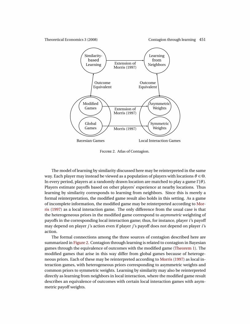
Morris (1997) identifies a formal relationship between contagion across types in incom-plete information games and contagion across players in local interaction games. Start-ing with some incomplete information game, one may reinterpret the types in the gameas players situated in various locations. Each of these players interacts with some sub-set of the population, her neighbors, and must choose the same action against all oppo-nents. Payoffs in the local interaction game are obtained by a weighted sum of payoffsfrom interactions with all neighbors, where the weights correspond to the posterior be-liefs over opponents’ types in the incomplete information game (see Morris 1997 fordetails).

12In addition, Samuelson and Zhang (1992), Nachbar (1990), and Heifetz et al. (2007) identify classes oflearning processes under which players learn not to play serially dominated strategies. However, all threepapers assume finite or real-valued strategy spaces. The strategy space in our environment, consisting offunctions s :Θ−→0, 1, is larger.


Bayesian Games

GlobalGames

ModifiedGames Extension of

Morris (1997)

Morris (1997)

Local Interaction Games

SymmetricWeights

AsymmetricWeights

OutcomeEquivalent

OutcomeEquivalent

Similarity-based

Learning Extension ofMorris (1997)

Learningfrom

Neighbors

F 2. Atlas of Contagion.

The model of learning by similarity discussed here may be reinterpreted in the sameway. Each player may instead be viewed as a population of players with locations θ ∈Θ.In every period, players at a randomly drawn location are matched to play a game Γ(θ ).Players estimate payoffs based on other players’ experience at nearby locations. Thuslearning by similarity corresponds to learning from neighbors. Since this is merely aformal reinterpretation, the modified game result also holds in this setting. As a gameof incomplete information, the modified game may be reinterpreted according to Mor-ris (1997) as a local interaction game. The only difference from the usual case is thatthe heterogeneous priors in the modified game correspond to asymmetric weighting ofpayoffs in the corresponding local interaction game; thus, for instance, player i ’s payoffmay depend on player j ’s action even if player j ’s payoff does not depend on player i ’saction.

The formal connections among the three sources of contagion described here aresummarized in Figure 2. Contagion through learning is related to contagion in Bayesiangames through the equivalence of outcomes with the modified game (Theorem 1). Themodified games that arise in this way differ from global games because of heteroge-neous priors. Each of these may be reinterpreted according to Morris (1997) as local in-teraction games, with heterogeneous priors corresponding to asymmetric weights andcommon priors to symmetric weights. Learning by similarity may also be reinterpreteddirectly as learning from neighbors in local interaction, where the modified game resultdescribes an equivalence of outcomes with certain local interaction games with asym-metric payoff weights.


7.2 Learning with incomplete information

An earlier version of this paper (Steiner and Stewart 2007) considers learning by similar-ity in games with incomplete information. The environment is close to that of Section 5,except that each player receives only a noisy signal x i

t = θt +σεit of the state θt in each

period t . Players estimate payoffs based on payoffs from similar past types. The mod-ified game result of Theorem 1 extends naturally to this setting, and may be used todemonstrate that there is a unique outcome of learning when both σ and τ are small(i.e. the noise in signals is small and players use narrow similarity functions). This out-come depends on the ratioσ/τ. Ifσ is small relative to τ, then we recover the completeinformation learning outcome of Proposition 1. Ifσ is large relative toτ, then we recoverthe usual global game solution.

8. C

The theory of global games has shown that relaxing the common knowledge assumptionin games can lead to a process of contagion that generates a unique selection amongmultiple equilibria. This paper identifies a similar effect that arises under learning if werelax the assumption that players learn from repeated play in exactly the same game.Moreover, the learning outcome is formally related to the equilibrium of a global gamewith subjective priors, which we call the modified game. While the connection to themodified game is very general, the set of learning outcomes may be difficult to identifyin games outside the coordination environment studied here. The unique outcome oflearning in this environment relies on the dominance solvability of the modified game.In more general settings, learning outcomes correspond to rationalizable profiles of thegame when beliefs are perturbed in a particular way that depends on the similarity func-tion. In a different setting, Weinstein and Yildiz (2007) show that for any finite type,given any rationalizable action, there exists a perturbation of beliefs in the universaltype space for which this action is uniquely rationalizable. A natural question, then, iswhether the corresponding result holds under learning by similarity in general classesof games; in other words, given any state in the original game, whether any equilibriummay be uniquely selected by an appropriate choice of similarity function.

A

L A.1. For any ε > 0, there exists some δ > 0 such that changing the opponents’strategies on a set of type profiles of Lebesgue measure at most δ changes the expectedpayoff of every type of player i from each action a i by at most ε.

P. Denote i ’s expected payoff from action a i at type θ against the profile s−i by

U i (θ , a i , s−i ) =

∫

Θu i (θ , a i , v i (θ ′, a i , s−i (θ ′)))φ(θ ′)g i (θ ′,θ )dθ ′

∫

Θφ(θ )g i (θ ,θ )d θ

.

The denominator is bounded above zero because it is continuous and positive by As-sumption A3, and hence attains a positive minimum on the compact set Θ. Recall that


the functions u i , g i , and φ are bounded by assumption. Hence there exists a constantK such that if s−i changes only on a set of measure δ, then the numerator changes by atmost Kδ.

L A.2. Fix a profile a and an arbitrary action a i . For any δ > 0, there exists someπ > 0 such that the set of types of player i for which action a i is dominated but not π-dominated under the profile a has measure at most δ.

P. Consider any decreasing sequence π1,π2, . . . such that limn→∞πn = 0. LetΘ(n )denote the set of types for which action a i is πn -dominated under a, and let Θ denotethe set of types for which a i is dominated under a. Then Θ(n ) is a monotone sequenceof sets, and it suffices to show that limn→∞Θ(n ) =Θ.

Suppose for contradiction thatΘ\limn→∞Θ(n ) contains some type θ . Then there ex-ists some action a i ′ that dominates a i at θ under the profile a, but does notπ-dominatea i at θ under a for any π> 0. Hence we have

infs−i∈a−i

U i (θ , a i ′, s−i )−U i (θ , a i , s−i ) = 0,

where we abuse notation by writing s−i ∈ a−i to mean that s−i is consistent with a−i .Define a strategy profile s−i by choosing

s−i (θ ′)∈ arg mina−i∈a−i (θ ′)

u i (θ , a i ′, v i (θ ′, a i ′, a−i ))−u i (θ , a i , v i (θ ′, a i , a−i ))

for each θ ′. The profile s−i is consistent with a−i , and satisfies

U i (θ , a i ′, s−i )−U i (θ , a i , s−i ) = infs−i∈a−i

U i (θ , a i ′, s−i )−U i (θ , a i , s−i ) = 0,

contradicting that a i ′ dominates a i at θ under a.

L A.3. For any k and θ , we have aik ,π(θ )⊆ ai

k ,π′ (θ )whenever π≤π′.P. Note that the statement is trivial for k = 0. Suppose for induction that the state-ment holds for k (for all θ ). We need to show that if a i is π′-dominated at θ under ak ,π′

then a i is π-dominated at θ under ak ,π. Accordingly, suppose that a i is π′-dominatedat θ under ak ,π′ ; that is, there exists a i ′ ∈ ai

k ,π′ for which

U (θ , a i ′, s−i )−U (θ , a i , s−i )>π′ for all s−i consistent with a−ik ,π′ . (12)

Since, by the inductive hypothesis, we have a−ik ,π ⊆ a−i

k ,π′ , (12) implies

U (θ , a i ′, s−i )−U (θ , a i , s−i )>π for all s−i consistent with a−ik ,π. (13)

If a i ′ ∈ aik ,π(θ ), then we are done. Otherwise, there exists some a i ′′ ∈ ai

k ,π(θ ) such thata i ′′ dominates a i ′ at θ under the profile ak ,π. Thus we have

U (θ , a i ′′, s−i )−U (θ , a i ′, s−i )> 0 for all s−i consistent with a−ik ,π.

Combining this with (13) gives the result.


P L . Given any type θ for which a i ∈ aik−1,0 \ ai

k ,0, there exists some

π(θ )> 0 such that, against any profile s−i consistent with a−ik−1,0, the expected payoff for

some action a i ′ ∈ aik ,0(θ ) is at least π(θ ) greater than that for action a i . By Lemma A.3,

we have a i ′ ∈ aik ,π(θ ) for all π > 0, and hence it suffices to show that a i ′ dominates a i

under the profile ak−1,π for some π> 0. By Lemma A.1, it suffices to show that given anyδ > 0, there exists some π> 0 small enough so that, for any player i , ai

k−1,π differs from

aik−1,0 on a set of measure at most δ.

We proceed by induction. The result is trivial for k = 1. For k > 1, assume for induc-tion that the result is true for k − 1; that is, assume that for any δ > 0, there exists someπ> 0 for which ai

k−2,π differs from aik−2,0 on a set of measure at most δ.

By Lemma A.2, given δ > 0, we can choose π′ > 0 small enough so that the set oftypes of player i for which the action a i is dominated but notπ′-dominated under ak−2,0

has measure at most δ. By Lemma A.1, starting from any strategy profile, there existssome δ′ > 0 such that changing the actions of at most a measure of δ′ of the opponents’types changes the expected payoff of each type of player i by at most π′/4. By the in-ductive hypothesis, we can choose π′′ > 0 such that a−i

k−2,π′′ differs from a−ik−2,0 on a set of

types of measure at most δ′. Consider π =minπ′/2,π′′. We need to show that aik−1,π

differs from aik−1,0 on a set of types of measure at most δ.

Consider any type θ and actions a i , a i ′ ∈ a−ik−2,0(θ ). By Lemma A.3, a i and a i ′ also

belong to a−ik−2,π(θ ) for all π > 0. Also by Lemma A.3, a−i

k−2,π(θ′) ⊆ a−i

k−2,π′′ (θ′) for all θ ′.

Therefore, we have

sups−i∈a−i

k−2,π

[U (θ , a i , s−i )−U (θ , a i ′, s−i )]≤ sups−i∈a−i

k−2,π′′[U (θ , a i , s−i )−U (θ , a i ′, s−i )], (14)

where, as above, we write s−i ∈ a−ik ,π to mean that the strategy profile s−i is consistent

with a−ik ,π. By the definition of π′′, we have

sups−i∈a−i

k−2,π′′[U (θ , a i , s−i )−U (θ , a i ′, s−i )]

≤ sups−i∈a−i

k−2,0

[U (θ , a i , s−i )−U (θ , a i ′, s−i )+ 12π′]. (15)

If action a i is π′-dominated by a i ′ for type θ of player i under ak−2,0, then

sups−i∈a−i

k−2,0

U (θ , a i , s−i )−U (θ , a i ′, s−i )+ 12π′<− 1

2π′.

Combining (14) and (15) gives the following: if action a i is π′-dominated for i at typeθ under ak−2,0, then a i must be π′/2-dominated, and hence also π-dominated underak−2,π. Therefore, if, at some θ , a i is dominated under ak−2,0 but not π-dominated un-der ak−2,π, then a i is dominated under ak−2,0 but not π′-dominated under ak−2,0. Thelatter can happen only on a set of types of measure δ.


We have shown that the set of types θ for which a i ∈ aik−2,π(θ ) but a i /∈ ai

k−2,0(θ ) hasmeasure at most δ. The result now follows since the number of players and the numberof actions are both finite.

P T . (i) Assume for induction that there almost surely exists some pe-riod after which the strategies s i

t are consistent with aik−1,π .

In the first step, we consider payoff estimates at a fixed state θ ∗. Suppose that actiona i is π-dominated by some action a i ′ for type θ ∗ of player i in the modified game underthe profile ak−1,π. Let

π′(θ ∗) =π∫

Θ

g i (θ ,θ ∗)dΦ(θ ).

We show that, under the learning process, there almost surely exists some period afterwhich the estimated payoff to action a i ′ at θ ∗ exceeds that to action a i by at leastπ. Thisis the case if

1

t

∑

s<t

u i (θ ∗, a i ′, v i (θs , a i ′, a−is ))−u i (θ ∗, a i , v i (θs , a i , a−i

s ))

g i (θs ,θ ∗)>π′(θ ∗). (16)

For each θ , θ ′ and a−i , let

∆(θ ,θ ′, a−i ) = u i (θ , a i ′, v i (θ ′, a i ′, a−i ))−u i (θ , a i , v i (θ ′, a i , a−i )).

Keeping θ ∗ fixed, choose the strategy profile s−imin(θ ) to minimize the payoff advantage

of a i ′ over a i at θ ∗; that is,

s−imin(θ )∈ arg min

a−i∈a−ik−1,π(θ )

∆(θ ∗,θ , a−i ).

Define a random variable

X =∆(θ ∗,θ , s−imin(θ ))g

i (θ ,θ ∗),

where the distribution of X is induced from the distribution Φ of θ .By the inductive hypothesis, opponents play actions in a−i

k−1,π(θs ) in every periods ≥ t0 for some t0. For large enough t > t0, periods up to t0 receive an arbitrarily smallweight in each player’s payoff estimates. Thus assuming that a−i

s ∈ a−ik−1,π(θs ) for all

s introduces only an arbitrarily small error in the payoff estimates. Note that for anyhistory (θs , a i

s , a−is )

t−1s=1 in which a−i

s ∈ a−ik−1,π(θs ), we have

1

t

∑

s<t

∆(θ ∗,θs , a−is )g

i (θs ,θ ∗)≥ 1

t

∑

s<t

∆(θ ∗,θs , s−imin(θs ))g i (θs ,θ ∗),

so it suffices to prove that (16) holds when a−is = s−i

min(θs ) for every s .By the Strong Law of Large Numbers, the weighted payoff difference

1

t

∑

s<t

∆(θ ∗,θs , s−imin(θs ))g i (θs ,θ ∗)


almost surely tends to the expectation of X , that is, to

∫

Θ

∆(θ ∗,θ , s−imin(θ ))g

i (θ ,θ ∗)dΦ(θ ).

By the assumption that a i ′ π-dominates a i , the last expression is greater than π′(θ ∗).Therefore, there almost surely exists some period T such that (16) holds for every t > T ,as desired.

In the second step, we show that there exists some δ> 0 such that if (16) holds at θ ∗,then s i

t (θ ) 6= a i for all θ ∈ (θ ∗−δ,θ ∗+δ). Let

π′ = infθ∈Θπ′(θ ).

By Assumption A3,π′(θ ) is positive everywhere, and since it is continuous, the compact-ness of Θ guarantees that π′ is bounded away from zero.

Define the function

k (h t ,θ ) =1

t

∑

s<t

u i (θ , a i ′, v i (θs , a i ′, a−is ))−u i (θ , a i , v i (θs , a i , a−i

s ))

g i (θs ,θ )

=1

t

∑

s<t

∆(θ ,θs , a−is )g

i (θs ,θ )

for finite histories h t = (θs , a is , a−i

s )s<t and states θ . Player i does not choose action a i

at state θ following history h t if k (h t ,θ ) > 0. Thus the second step will be complete ifwe show that, for some δ> 0, after any history h t , we have

k (h t ,θ )−k (h t ,θ ′)

<π′

whenever |θ −θ ′|<δ.By Assumption A4,∆(θ ,θs , a−i

s )gi (θs ,θ ) is uniformly continuous in θ over all θs and

a−is . Hence the average k (h t ,θ ) is also continuous in θ uniformly over all values of θ and

all histories h t , as needed.Finally, partition the setΘ into a finite number of subsetsΘ1, . . . ,Θm , each of diame-

ter less than δ (where δ is chosen given π′ as in the second step above). Consider any ofthese subsetsΘl . IfΘl contains some θ ∗ at which a i is π-dominated by a i ′ (under someprofile), then by the first step, k (h t ,θ ∗) is eventually larger than π′. By the second step,k (h t ,θ ) is therefore positive for all types in Θl . Hence there almost surely exists someperiod Tl after which player i never plays action a i at any state in Θl . Since there areonly finitely many sets Θl , there almost surely exists some T after which player i neverplays action a i at any state θ for which it is serially π-dominated for the correspondingtype in the modified game. The result now follows from the finiteness of the action andplayer sets.

(ii) First we claim that for any k , the probability that play is consistent with k roundsof IEDS in the modified game approaches one as time tends to infinity. In the proofof Lemma 1, we show that for any δ > 0, there exists some π > 0 such that the set of


types θ at which k rounds of IEDS differ from k rounds of IEπDS has measure at mostδ. Thus the probability that θt lies in this set can be made arbitrarily small by choosingπ to be sufficiently small. Note that outside of this set, play under the learning processis almost surely eventually consistent with k rounds of IEDS by part (i) of the theorem.This proves the claim.

For each k = 1, 2, . . ., denote by Θik the set of types of player i for which all se-

rially dominated actions are eliminated within the first k rounds of IEDS. Let Θk =⋂

i=1,...,I Θik . The sequence of sets Θk is nondecreasing in k , and converges to the set

Θ. Hence the measure of the set Θ \Θk converges to zero as k tends to infinity. Fromthe previous paragraph, the probability that play is consistent with IEDS onΘk tends toone over time, and the probability that the state θt lies inΘ \Θk can be made arbitrarilysmall by choosing k to be sufficiently large.

R

Argenziano, Rossella and Itzhak Gilboa (2005), “History as a coordination device.” Un-published paper, Department of Economics, University of Essex. [450]

Beggs, Alan (2005), “Learning in Bayesian games with binary actions.” Economics SeriesWorking Paper 232, University of Oxford, Department of Economics. [450]

Carlsson, Hans (2004), “Rational and adaptive play in two-person global games.” Un-published paper, Department of Economics, Lund University. [443, 450]

Carlsson, Hans and Eric van Damme (1993), “Global games and equilibrium selection.”Econometrica, 61, 989–1018. [433, 434, 436]

Eyster, Erik and Matthew Rabin (2005), “Cursed equilibrium.” Econometrica, 73, 1623–1672. [449]

Frankel, David M., Stephen Morris, and Ady Pauzner (2003), “Equilibrium selection inglobal games with strategic complementarities.” Journal of Economic Theory, 108, 1–44.[444]

Germano, Fabrizio (2007), “Stochastic evolution of rules for playing finite normal formgames.” Theory and Decision, 62, 311–333. [449]

Gilboa, Itzhak and David Schmeidler (2001), A Theory of Case-Based Decisions. Cam-bridge University Press, Cambridge. [433]

Heifetz, Aviad, Chris Shannon, and Yossi Spiegel (2007), “The dynamic evolution of pref-erences.” Economic Theory, 32, 251–286. [450]

Izmalkov, Sergei and Muhamet Yildiz (2008), “Investor sentiments.” Unpublished paper,Department of Economics, Massachusetts Institute of Technology. [448]

Jehiel, Philippe (2005), “Analogy-based expectation equilibrium.” Journal of EconomicTheory, 123, 81–104. [447, 449]


Jehiel, Philippe and Frederic Koessler (2008), “Revisiting games of incomplete infor-mation with analogy-based expectations.” Games and Economic Behavior, 62, 533–557.[449]

Katz, Kimberly F. (1996), Three Applications of Game Theory. Ph.D. thesis, University ofPennsylvania. [449]

LiCalzi, Marco (1995), “Fictitious play by cases.” Games and Economic Behavior, 11, 64–89. [449]

Mengel, Friederike (2007), “Learning across games.” Working Paper WP-AD 2007-05, In-stituto Valenciano de Investigaciones Económicas. [449]

Milgrom, Paul and John Roberts (1990), “Rationalizability, learning, and equilibrium ingames with strategic complementarities.” Econometrica, 58, 1255–1277. [446, 450]

Morris, Stephen (1997), “Interaction games: A unified analysis of incomplete informa-tion, local interaction and random matching.” Working Paper 97-08-072, Santa Fe Insti-tute. [450, 451]

Morris, Stephen (2000), “Contagion.” Review of Economic Studies, 67, 57–78. [433]

Morris, Stephen and Hyun Song Shin (2003), “Global games: Theory and applications.”In Advances in Economics and Econometrics, Volume 1 (Mathias Dewatripont, Lars Pe-ter Hansen, and Stephen J. Turnovsky, eds.), 56–114, Cambridge University Press, Cam-bridge. [434, 445]

Nachbar, John H. (1990), “‘Evolutionary’ selection dynamics in games: Convergence andlimit properties.” International Journal of Game Theory, 19, 59–89. [450]

Samuelson, Larry and Jianbo Zhang (1992), “Evolutionary stability in asymmetricgames.” Journal of Economic Theory, 57, 363–391. [450]

Stahl, Dale O. and John Van Huyck (2002), “Learning conditional behavior in similar staghunt games.” Unpublished paper. [449]

Steiner, Jakub and Colin Stewart (2007), “Learning by similarity in coordination prob-lems.” Working Paper 324, Center for Economic Research and Graduate Education, Eco-nomics Institute, Charles University. [452]

Weinstein, Jonathan and Muhamet Yildiz (2007), “A structure theorem for rationalizabil-ity with application to robust predictions of refinements.” Econometrica, 75, 365–400.[452]

Submitted 2007-12-14. Final version accepted 2008-8-11. Available online 2008-8-20.

Documents

Contagionthroughlearning - University of Toronto T-Space · Contagionthroughlearning Jakub Steiner ... Ben Polak, Marzena Rostek, ... a function of a continuous variable using only