Constructivism Learning: A Learning Paradigm for

Constructivism Learning:A Learning Paradigm for Transparent Predictive Analytics

By

Xiaoli Li

Submitted to the graduate degree program in Department of Electrical Engineering and ComputerScience and the Graduate Faculty of the University of Kansas in partial fulfillment of the

requirements for the degree of Doctor of Philosophy.

Committee members

Jun Huan, Committee Chair

Victor S. Frost, Committee Member

Bo Luo, Committee Member

Guanghui Wang, Committee Member

Alfred Tat-Kei Ho, Committee Member

Date defended:

The Thesis Committee for Xiaoli Li certifiesthat this is the approved version of the following thesis :

Constructivism Learning:A Learning Paradigm for Transparent Predictive Analytics

Jun Huan, Committee Chair

Date approved:

ii

Acknowledgements

Sincere gratitude and appreciation are extended to my advisor, Dr. Huan, for his guidance, which

points me to the moon, and his consistent support through my Ph.D. study. I also would like to

express my gratitude to my committee members, Dr. Frost, Dr. Luo, Dr. Wang, and Dr. Ho, for

their help and valuable time.

The ITTC help team also deserves my warmest thanks. They are always ready to help. Without

their timely support, it will be difficult for me to finish all the experiments in this work.

My last thanks go to my friends who have accompanied me and encouraged me through this

long journey.

iii

Abstract

Aiming to achieve the learning capabilities possessed by intelligent beings, especially

human, researchers in machine learning field have the long-standing tradition of bor-

rowing ideas from human learning, such as reinforcement learning, active learning,

and curriculum learning. Motivated by a philosophical theory called "constructivism",

in this work, we propose a new machine learning paradigm, constructivism learning.

The constructivism theory has had wide-ranging impact on various human learning

theories about how human acquire knowledge. To adapt this human learning theory

to the context of machine learning, we first studied how to improve leaning perfor-

mance by exploring inductive bias or prior knowledge from multiple learning tasks

with multiple data sources, that is multi-task multi-view learning, both in offline and

lifelong setting. Then we formalized a Bayesian nonparametric approach using se-

quential Dirichlet Process Mixture Models to support constructivism learning. To fur-

ther exploit constructivism learning, we also developed a constructivism deep learning

method utilizing Uniform Process Mixture Models.

iv

Contents

1 Introduction 1

2 Nailing Interactions in Multi-Task Multi-View Multi-Label Learning 5

2.1 Introduction . . . . . . . . . . . . . . . . . . . . . . . . . . . . . . . . . . . . . . 5

2.2 Related work . . . . . . . . . . . . . . . . . . . . . . . . . . . . . . . . . . . . . 8

2.2.1 Bilinear Factor Analysis and Multilinear Factor Analysis . . . . . . . . . . 8

2.2.2 MTVL Learning . . . . . . . . . . . . . . . . . . . . . . . . . . . . . . . 9

2.2.3 MTV Learning . . . . . . . . . . . . . . . . . . . . . . . . . . . . . . . . 9

2.3 Preliminary . . . . . . . . . . . . . . . . . . . . . . . . . . . . . . . . . . . . . . 10

2.3.1 Notation . . . . . . . . . . . . . . . . . . . . . . . . . . . . . . . . . . . 10

2.3.2 Definitions for Tensors . . . . . . . . . . . . . . . . . . . . . . . . . . . . 10

2.3.3 Probabilistic Multilinear Factor Analyzers (MLFA) . . . . . . . . . . . . . 13

2.4 Algorithm . . . . . . . . . . . . . . . . . . . . . . . . . . . . . . . . . . . . . . . 14

2.4.1 Problem Formulation . . . . . . . . . . . . . . . . . . . . . . . . . . . . . 15

2.4.2 MTVL Learning with Task-View-Label Interactions . . . . . . . . . . . . 15

2.4.2.1 Adaptive-basis Multilinear Factor Analyzers (aptMLFA) . . . . . 16

2.4.2.2 MTVL Learning using aptMLFA (aptMTVL) . . . . . . . . . . 18

2.4.2.3 Optimization for aptMTVL . . . . . . . . . . . . . . . . . . . . 21

2.4.3 MTVL Learning without Interactions

(aptMTVL−) . . . . . . . . . . . . . . . . . . . . . . . . . . . . . . . . . 23

2.5 Experimental Studies . . . . . . . . . . . . . . . . . . . . . . . . . . . . . . . . . 26

2.5.1 Data Sets . . . . . . . . . . . . . . . . . . . . . . . . . . . . . . . . . . . 28

2.5.2 Experimental Protocol . . . . . . . . . . . . . . . . . . . . . . . . . . . . 29

v

2.5.3 Experimental Results and Discussion . . . . . . . . . . . . . . . . . . . . 30

2.6 Conclusion . . . . . . . . . . . . . . . . . . . . . . . . . . . . . . . . . . . . . . 31

3 Multilinear Dirichlet Processes 32

3.1 Introduction . . . . . . . . . . . . . . . . . . . . . . . . . . . . . . . . . . . . . . 32

3.2 Related Work . . . . . . . . . . . . . . . . . . . . . . . . . . . . . . . . . . . . . 34

3.3 Preliminary . . . . . . . . . . . . . . . . . . . . . . . . . . . . . . . . . . . . . . 34

3.3.1 Notations . . . . . . . . . . . . . . . . . . . . . . . . . . . . . . . . . . . 35

3.3.2 Basic definitions for Tensors . . . . . . . . . . . . . . . . . . . . . . . . . 35

3.3.3 Multilinear Factor Analyzers . . . . . . . . . . . . . . . . . . . . . . . . . 35

3.4 Algorithm . . . . . . . . . . . . . . . . . . . . . . . . . . . . . . . . . . . . . . . 36


3.4.2 Multilinear Dirichlet Processes . . . . . . . . . . . . . . . . . . . . . . . . 37

3.4.3 MLDP Mixture of Models . . . . . . . . . . . . . . . . . . . . . . . . . . 40

3.4.4 Computation . . . . . . . . . . . . . . . . . . . . . . . . . . . . . . . . . 41


3.5.1 Density Estimation . . . . . . . . . . . . . . . . . . . . . . . . . . . . . . 45

3.5.2 Multilinear Multi-task Learning (MLMTL) . . . . . . . . . . . . . . . . . 47

3.5.3 Context-aware Recommendation . . . . . . . . . . . . . . . . . . . . . . . 49

3.5.4 Time Performance Evaluation . . . . . . . . . . . . . . . . . . . . . . . . 50

3.6 Conclusion . . . . . . . . . . . . . . . . . . . . . . . . . . . . . . . . . . . . . . 51

4 Lifelong Multi-task Multi-view Learing 52

4.1 Introduction . . . . . . . . . . . . . . . . . . . . . . . . . . . . . . . . . . . . . . 52

4.2 Related Work . . . . . . . . . . . . . . . . . . . . . . . . . . . . . . . . . . . . . 54

4.3 Algorithm . . . . . . . . . . . . . . . . . . . . . . . . . . . . . . . . . . . . . . . 55

4.3.1 Notations . . . . . . . . . . . . . . . . . . . . . . . . . . . . . . . . . . . 55


vi

4.3.3 Latent Space MTMV Learning . . . . . . . . . . . . . . . . . . . . . . . . 56

4.3.4 Latent Space MTMV Learning Details . . . . . . . . . . . . . . . . . . . . 59

4.3.5 Latent Space Lifelong MTMV learning . . . . . . . . . . . . . . . . . . . 60


4.4.1 Datasets . . . . . . . . . . . . . . . . . . . . . . . . . . . . . . . . . . . . 67



4.4.3.1 Performance Comparison of Offline Algorithms . . . . . . . . . 70

4.4.3.2 Performance Comparison of Lifelong Learning Algorithms . . . 71

4.4.3.3 Training Time Comparison . . . . . . . . . . . . . . . . . . . . 71

4.5 Conclusion . . . . . . . . . . . . . . . . . . . . . . . . . . . . . . . . . . . . . . 74

5 Constructivism Learning 75

5.1 introduction . . . . . . . . . . . . . . . . . . . . . . . . . . . . . . . . . . . . . . 75

5.2 Related Work . . . . . . . . . . . . . . . . . . . . . . . . . . . . . . . . . . . . . 77

5.2.1 Transparent Machine Learning . . . . . . . . . . . . . . . . . . . . . . . . 78

5.2.2 Constructivism Learning . . . . . . . . . . . . . . . . . . . . . . . . . . . 78

5.2.3 Learning with Task Construction . . . . . . . . . . . . . . . . . . . . . . . 78

5.3 Preliminary . . . . . . . . . . . . . . . . . . . . . . . . . . . . . . . . . . . . . . 79

5.3.1 Dirichlet Process Mixtures . . . . . . . . . . . . . . . . . . . . . . . . . . 79

5.3.2 Sequential DP Mixture Models (sDPMM) . . . . . . . . . . . . . . . . . . 81

5.4 Algorithm . . . . . . . . . . . . . . . . . . . . . . . . . . . . . . . . . . . . . . . 82

5.4.1 Notation . . . . . . . . . . . . . . . . . . . . . . . . . . . . . . . . . . . 82

5.4.2 Problem Setting and Challenges . . . . . . . . . . . . . . . . . . . . . . . 83

5.4.3 Sequential DP Mixture of Classification Model . . . . . . . . . . . . . . . 84

5.4.3.1 DP Mixture of Classification Model . . . . . . . . . . . . . . . . 85

5.4.3.2 Variational Approximation of Logistic Regression . . . . . . . . 86

vii

5.4.4 Sequential DP Mixture of Classification Model with Selection Principle

(sDPMCM-s) . . . . . . . . . . . . . . . . . . . . . . . . . . . . . . . . . 88

5.4.4.1 Selection Principle . . . . . . . . . . . . . . . . . . . . . . . . . 88

5.4.4.2 Applying Selection principle . . . . . . . . . . . . . . . . . . . 89

5.4.5 Inference . . . . . . . . . . . . . . . . . . . . . . . . . . . . . . . . . . . 89

5.4.5.1 Utility Computation . . . . . . . . . . . . . . . . . . . . . . . . 90

5.4.5.2 Sequential Inference for sDPMCM-s . . . . . . . . . . . . . . . 90

5.4.5.3 Prediction . . . . . . . . . . . . . . . . . . . . . . . . . . . . . 92


5.5.1 Data Sets . . . . . . . . . . . . . . . . . . . . . . . . . . . . . . . . . . . 92

5.5.1.1 Synthetic Data Sets . . . . . . . . . . . . . . . . . . . . . . . . 93

5.5.1.2 Real-world Data Sets . . . . . . . . . . . . . . . . . . . . . . . 93

5.5.2 Experiment Protocol . . . . . . . . . . . . . . . . . . . . . . . . . . . . . 94

5.5.3 Performance Evaluation Results . . . . . . . . . . . . . . . . . . . . . . . 95

5.5.3.1 Comparison on Synthetic Data Sets . . . . . . . . . . . . . . . . 95

5.5.3.2 Comparison on Real Data Sets . . . . . . . . . . . . . . . . . . 96

5.5.4 Transparency Evaluation . . . . . . . . . . . . . . . . . . . . . . . . . . . 97

5.5.4.1 Evaluation on Synthetic Data Sets . . . . . . . . . . . . . . . . . 97

5.5.4.2 Evaluation on Real-World Data Sets . . . . . . . . . . . . . . . 97

5.6 Conclusion . . . . . . . . . . . . . . . . . . . . . . . . . . . . . . . . . . . . . . 99

6 Constructivism Learning for Local Dropout Architecture Construction 100

6.1 Introduction . . . . . . . . . . . . . . . . . . . . . . . . . . . . . . . . . . . . . . 100

6.2 Related Work . . . . . . . . . . . . . . . . . . . . . . . . . . . . . . . . . . . . . 103

6.2.1 Dropout Training for Deep Neural Networks . . . . . . . . . . . . . . . . 103

6.2.2 Constructivism Learning in Machine Learning . . . . . . . . . . . . . . . 104

6.3 Preliminary . . . . . . . . . . . . . . . . . . . . . . . . . . . . . . . . . . . . . . 104

6.3.1 Notations . . . . . . . . . . . . . . . . . . . . . . . . . . . . . . . . . . . 105

viii

6.3.2 Uniform Process . . . . . . . . . . . . . . . . . . . . . . . . . . . . . . . 105

6.4 Algorithm . . . . . . . . . . . . . . . . . . . . . . . . . . . . . . . . . . . . . . . 106

6.4.1 Constructivism Learning for Local Dropout Architecture Construction (CODA)107

6.4.2 UP Mixture Models for CODA . . . . . . . . . . . . . . . . . . . . . . . . 108

6.4.3 Computation . . . . . . . . . . . . . . . . . . . . . . . . . . . . . . . . . 111

6.4.3.1 Update architecture Assignment . . . . . . . . . . . . . . . . . . 111

6.4.3.2 Update Z . . . . . . . . . . . . . . . . . . . . . . . . . . . . . . 113

6.4.3.3 Update W . . . . . . . . . . . . . . . . . . . . . . . . . . . . . 114

6.4.3.4 Prediction . . . . . . . . . . . . . . . . . . . . . . . . . . . . . 115

6.5 Experiments . . . . . . . . . . . . . . . . . . . . . . . . . . . . . . . . . . . . . . 116

6.5.1 Data Sets . . . . . . . . . . . . . . . . . . . . . . . . . . . . . . . . . . . 116

6.5.1.1 Synthetic Data Sets . . . . . . . . . . . . . . . . . . . . . . . . 116

6.5.1.2 Real-world Data Sets . . . . . . . . . . . . . . . . . . . . . . . 117

6.5.2 Compared Methods . . . . . . . . . . . . . . . . . . . . . . . . . . . . . . 118



6.5.4.1 Optimization Evaluation . . . . . . . . . . . . . . . . . . . . . . 120

6.5.4.2 Performance Evaluation . . . . . . . . . . . . . . . . . . . . . . 122

6.5.4.3 Case Study . . . . . . . . . . . . . . . . . . . . . . . . . . . . . 123

6.6 Conclusion . . . . . . . . . . . . . . . . . . . . . . . . . . . . . . . . . . . . . . 124

7 Conclusion 125

A Proof and Optimization for Chapter 2 142

A.1 Proof of Proposition 3 . . . . . . . . . . . . . . . . . . . . . . . . . . . . . . . . . 142

A.2 Proof of Proposition 4 . . . . . . . . . . . . . . . . . . . . . . . . . . . . . . . . . 144

A.2.1 Proof of Proposition 5 . . . . . . . . . . . . . . . . . . . . . . . . . . . . 146

A.3 Optimization . . . . . . . . . . . . . . . . . . . . . . . . . . . . . . . . . . . . . 147

ix

A.3.1 Optimization for pt . . . . . . . . . . . . . . . . . . . . . . . . . . . . . . 147

A.3.2 Optimization for qv . . . . . . . . . . . . . . . . . . . . . . . . . . . . . . 149

A.3.3 Optimization for sl . . . . . . . . . . . . . . . . . . . . . . . . . . . . . . 150

x

List of Figures

2.1 Illustration of n-mode fibers. I: a tensor A ∈ R2×3×2, II:1-mode (column) fibers,

III:2-mode (row) fibers, IV:3-mode (tube) fibers. . . . . . . . . . . . . . . . . . . . 12

2.2 Performance Comparison w/o Task-view-label Interactions . . . . . . . . . . . . . 30

3.1 Form Left to Right: 1. SDS1; 2. SDS2; 3.SDS3. . . . . . . . . . . . . . . . . . . . 46

3.2 Form Left to Right: 1. MLMTL on Restaurant & Consumer Data set; 2. MLMTL

on School Data set; 3. CARS on Frappe Data Set; 4. CARS on Japan Restaurant

Data Set. Algorithms: a. DP-MRM; b: MXDP-MRM; c: ANOVADP-MRM; d:

MLMTL-C; e:TPG; f: CSLIM; g:MLDP-MRM . . . . . . . . . . . . . . . . . . . 46

4.1 Lifelong Learning Problem . . . . . . . . . . . . . . . . . . . . . . . . . . . . . . 57

4.2 Latent Space MTMV Learning . . . . . . . . . . . . . . . . . . . . . . . . . . . . 58

4.3 Training time comparison of different algorithms on synthetic data set with varying

number of features from 100 to 1000. Left: Comparison of lslMTMV with other

three baseline algorithms. Right: Comparison of lslMTMV with CoRegMTMV . . 73

4.4 Training time comparison of different algorithms on synthetic data set with vary-

ing number of tasks from 10 to 100. Left: Comparison of lslMTMV with other

three baseline algorithms. Middle: Comparison of lslMTMV with ELLA. Right:

Performance of lslMTMV . . . . . . . . . . . . . . . . . . . . . . . . . . . . . . 73

4.5 Training time comparison of different algorithms on synthetic data set with varying

number of views from 2 to 20. Left: Comparison of lslMTMV with CoRegMTMV

and MAMUDA. Right: Performance of lslMTMV . . . . . . . . . . . . . . . . . . 74

xi

5.1 Issue of Fitness Principle: Left: Gound Truth; Middle: Tasks Constructed without

Using the Fitness Principle; Right: Tasks Constructed using the Selection Principle. 84

5.2 Function of Selection Principle: s1: mean of positive samples; s2: mean of negative

samples; s3: close to decision boundary; s4; far away from decision boundary. . . . 89

5.3 Transparency Evaluation on Synthetic Data Set SDS2. Top: SVM, Middle: Ran-

dom Forest, Bottom: sDPMCM-s. . . . . . . . . . . . . . . . . . . . . . . . . . . 98

5.4 Tasks Construction Comparison: Left: Ground Truth, Middle: Tasks Constructed

by sDPMCM, Right: Tasks Constructed by sDPMCM-s . . . . . . . . . . . . . . . 98

5.5 Transparency Evaluation on School Data Set. Top: SVM, Middle: Random Forest,

Bottom: sDPMCM-s. . . . . . . . . . . . . . . . . . . . . . . . . . . . . . . . . . 98

6.1 Constructivism Deep Learning. Left: The Network Architecture of a DNN. Middle

and Right: Two Different Dropout Architectures. The first dropout architecture is

shared by instances (x1,y1) and (x4,y4). The second dropout architecture is shared

by instances (x2,y2) and (x3,y3). . . . . . . . . . . . . . . . . . . . . . . . . . . . 102

6.2 Case Study. Group1: Recommended for Banquets; Group2: Not Recommended

for Banquets; Blue: Training with All Instances; Red: Training with Splitted In-

stances. . . . . . . . . . . . . . . . . . . . . . . . . . . . . . . . . . . . . . . . . 124

xii

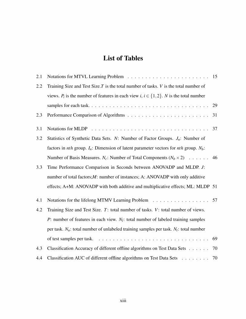
List of Tables

2.1 Notations for MTVL Learning Problem . . . . . . . . . . . . . . . . . . . . . . . 15

2.2 Training Size and Test Size.T is the total number of tasks. V is the total number of

views. Pi is the number of features in each view i, i ∈ 1,2. N is the total number

samples for each task. . . . . . . . . . . . . . . . . . . . . . . . . . . . . . . . . . 29

2.3 Performance Comparison of Algorithms . . . . . . . . . . . . . . . . . . . . . . . 31

3.1 Notations for MLDP . . . . . . . . . . . . . . . . . . . . . . . . . . . . . . . . . 37

3.2 Statistics of Synthetic Data Sets. N: Number of Factor Groups. Jn: Number of

factors in nth group. In: Dimension of latent parameter vectors for nth group. Nb:

Number of Basis Measures. Nc: Number of Total Components (Nb×2) . . . . . . 46

3.3 Time Performance Comparison in Seconds between ANOVADP and MLDP. J:

number of total factors;M: number of instances; A: ANOVADP with only additive

effects; A+M: ANOVADP with both additive and multiplicative effects; ML: MLDP 51

4.1 Notations for the lifelong MTMV Learning Problem . . . . . . . . . . . . . . . . 57

4.2 Training Size and Test Size. T : total number of tasks. V : total number of views.

P: number of features in each view. Nl: total number of labeled training samples

per task. Nu: total number of unlabeled training samples per task. Nt : total number

of test samples per task. . . . . . . . . . . . . . . . . . . . . . . . . . . . . . . . 69

4.3 Classification Accuracy of different offline algorithms on Test Data Sets . . . . . . 70

4.4 Classification AUC of different offline algorithms on Test Data Sets . . . . . . . . 70

xiii

4.5 Classification Accuracy of the lslMTMV algorithm with Different Training Meth-

ods and of ELLA algorithm on Test Data Sets. M1: Sequential Training. M2:

Round-robin Training. M3: Random Training. For comparison we duplicate the

classification accuracy and AUC data of lsMTMV. . . . . . . . . . . . . . . . . . . 71

4.6 Classification AUC of the lslMTMV algorithm with Different Training Methods

and of ELLA algorithm on Test Data Sets. . . . . . . . . . . . . . . . . . . . . . 72

5.1 Comparison of KLD and Posterior Predictive Probability (Pr) . . . . . . . . . . . . 88

5.2 Statistics of Synthetic Data Sets. T: Number of Hidden Tasks. N: Number of

Samples. . . . . . . . . . . . . . . . . . . . . . . . . . . . . . . . . . . . . . . . . 93

5.3 Statistics of Real Data Sets. N: number of samples d: number of features . . . . . . 94

5.4 Comparison of Algorithms on Synthetic Data Sets. AUC is used for the perfor-

mance metric.*: statistically significant with 5% significance level. . . . . . . . . . 96

5.5 Comparison of Algorithms on Real Data Sets. AUC is used for the performance

metric.*: statistically significant with 5% significance level. . . . . . . . . . . . . . 96

6.1 Notations for CODA . . . . . . . . . . . . . . . . . . . . . . . . . . . . . . . . . 106

6.2 Statistics of Synthetic Data Sets. N: Number of Instances, D: Number of features,

L: Number of Labels, U: number of hidden units in each hidden layer, K: number

of dropout architectures . . . . . . . . . . . . . . . . . . . . . . . . . . . . . . . . 117

6.3 Statistics of Real-world Data Sets. N: Number of Instances, D: Number of features,

L: Number of Labels. . . . . . . . . . . . . . . . . . . . . . . . . . . . . . . . . . 118

6.4 Optimization Evaluation on Synthetic Data Sets. **: statistically significant with

1% significance level; *: statistically significant with 5% significance level. . . . . 121

6.5 Optimization Evaluation on Real-world Data Sets . . . . . . . . . . . . . . . . . . 122

6.6 Model Performance using F1 score with Different Methods on Synthetic Data Sets 123

6.7 Model Performance using F1 score with Different Methods on Real-world Data Sets123

xiv

Chapter 1

Introduction

To implant learning capabilities possessed by intelligent beings, especially human, into computers,

machine learning researchers have strived for decades to acquire inspirations from various sources

and devise novel algorithms based on those inspirations. Among those different sources, one

important source is human intelligence and learning. Many lines of research in machine learning

can trace its underling ideas to this source, for example, reinforcement learning, active learning,

curriculum learning, and deep learning.

Following this long-standing tradition in machine learning, in this work, we try to simulate and

investigate the human learning situation where a learner will learn multiple tasks under different

cases. Specially, we aim to answer the following questions:

• How to model the interactions among different learning factors when those learning tasks

have information from multiple data sources with multiple labels or there exist a complex

structure among those tasks?

• How to gradually and efficiently improve the learning performance by borrowing knowledge

from previous learning when those tasks arrive over time?

• If those learning tasks are not predefined, how the learning algorithm can posses the capa-

bility to determine when a new task should be constructed for a new experience and acquire

new knowledge?

To answer those questions, we start our study from a new direction of multi-task multi-view

learning where we have data sets with multiple tasks, multiple views and multiple labels. We call

1

this problem a multi-task multi-view multi-label learning problem or MTVL learning for short.

There is a wide application of MTVL leaning where examples include Internet of Things, brain

science, and document classification. In designing effective MTVL learning algorithms, we hy-

pothesize that a key component is to “disentangle” interactions among tasks, views, and labels, or

the task-view-label interactions. For that purpose we have developed an adaptive-basis multilinear

analyzers(aptMLFA) that utilizes a loading tensor to modulate interactions among multiple latent

factors. With aptMLFA we designed a new MTVL learning algorithm, aptMTVL, and evaluated

its performance on 3 real-world data sets. The experimental results demonstrated the effectiveness

of our proposed method as compared to the state-of-the-art MTVL learning algorithm.

To accommodate the complex dependent structure that may exist in multiple tasks, we investi-

gate to utilize Dependent Dirichlet processes (DDP). DDP have been widely applied to model data

from distributions over collections of measures which are correlated in some way. However, few

researchers have addressed the heterogeneous relationship in data brought by modulation of mul-

tiple factors resulting from the complex dependent structure using techniques of DDP. To bridge

this gap, we propose a novel technique, MultiLinear Dirichlet Processes (MLDP), to construct

DDPs by combining DP with a state-of-the-art factor analysis technique, multilinear factor analyz-

ers (MLFA). We have evaluated MLDP on real-word data sets for different applications and have

achieved state-of-the-art performance.

To answer the second question, we study the problem of MTMV learning in a lifelong learn-

ing framework. Lifelong machine learning, like human lifelong learning, learns multiple tasks

over time. Lifelong multi-task multi-view (Lifelong MTMV) learning is a new data mining and

machine learning problem where new tasks and/or new views may come in anytime during the

learning process. Our goal is to efficiently learn a model for a new task or new view by selectively

transferring knowledge learned from previous tasks or views. To this end, we propose a latent

space lifelong MTMV (lslMTMV) learning method to exploit task relatedness and information

from multiple views. In this new method we map views to a shared latent space and then learn a

decision function in the latent space. Our new method supports knowledge sharing among mul-

2

tiple views and knowledge transfer from existing tasks to a new learning task naturally. We have

evaluated our method using 3 real-world data sets. The experimental study results demonstrate that

the classification accuracy of our algorithm is close or superior to state-of-the-art offline MTMV

learning algorithms while the time needed to training such models is orders of magnitude less.

Learning with multiple tasks is an effective way to exploit inductive bias or prior knowlege.

However, in human learning, it is often the situation that learning tasks are not predefined, which

raises the third question we mentioned before. In the meantime, we aim to achieve transparent

predictive analytics and understand the internal and often complicated modeling processes. To this

end, we adopt a contemporary philosophical concept called “constructivism”, which is a theory

regarding how human learns. We hypothesis that a critical aspect of transparent machine learn-

ing is to “reveal” model construction with two key process: (1) the assimilation process where

we enhance our existing learning models and (2) the accommodation process where we create

new learning models. With this intuition we propose a new learning paradigm using a Bayesian

nonparametric to dynamically handle the creation of new learning tasks. Our empirical study on

both synthetic and real data sets demonstrate that the new learning algorithm is capable of deliv-

ering higher quality models (as compared to base lines and state-of-the-art) and at the same time

increasing the transparency of the learning process.

To further exploit the advantage of constructivism learning, we also apply it to deep learning.

Specially, we propose a method called constructivism deep learning. Based on dropout, which

has attracted widespread interest due to its effectiveness in training deep neural networks, the goal

of constructivism deep learning is to determine whether a new dropout architecture or an existing

dropout architecture should be used for an instance. Mathematically, we design a method, Uniform

Process Mixture Models, based on a Bayesian nonparametric method, Uniform process. We have

evaluated our proposed method on 3 real-world datasets and compared the performance with other

state-of-the-art dropout techniques. The experimental results demonstrated the effectiveness of our

method.

The reminder of this work is organized as follows. In the first three chapters, we present our

3

research on three different learning problems related to learning with multiple tasks, multi-task

multi-view multi-label learning, multilinear multi-task learning, and lifelong multi-task learning.

Then we introduce our work on constructivism learning in chapter 5 and chapter 6. We conclude

the whole work in chapter 7.

4

Chapter 2

Nailing Interactions in Multi-Task Multi-View Multi-Label

Learning

2.1 Introduction

We investigate a new setting of multi-task multi-view (MTV) learning where we have multiple

related learning tasks. For each task the data is collected from multiple sources and is labeled

with more than one labels. We call this type of data analytics problems multi-task, multi-view, and

multi-label learning, or MTVL learning for short. Our research is motivated by the observation that

with the fast accumulation of big data there is a clear interaction between data sources, labels of

data, and learning tasks. Specifically we list a few examples of MTVL with real-world application

below.

• In the application of Internet of Things to targeted marketing of products and services, we

collect behavioral statistics of users who use various kinds of devices connected by Internet

to recommend products or services to users. We may treat each user as a task, the information

acquired through each kind of device as a view, and each type of product or service as a label.

Then we use MTVL learning techniques to construct personalized product recommendations

for users [Moss, 2015].

• To understand how the brain works, scientists often collect different types of features of

brain imaging. Examples include the firing activity of a neural circuit, the connectivity of the

circuit, and the functional or behavioral output of the circuit. These data is used to construct

predictive models to understand the set of objects that a human subject is thinking. If we

5

treat each experimental subject (i.e., a person) as a task, each object as a label, we formalize

this problem as a MTVL learning problem [Alivisatos et al., 2012, Wehbe et al., 2014].

• In hierarchical document classification the categories are organized in a tree. In order to

perform efficient categorization, we often collect multiple feature groups, each of which is

considered as a view. We then treat all leaf categories as labels and we may select some

internal nodes as tasks [Yang & He, 2015]. If we formalize the learning process as outlined

here we have a MTVL learning problem.

To the best of our knowledge Yang and He developed the first and the only MTVL algorithm,

hierarchical Multi-Latent Space Model(HiMLS) [Yang & He, 2015]. In HiMLS, the object-feature

matrices and object-label matrices are decomposed using a 3-way non-negative matrix factoriza-

tion. Task-view interactions and task-label interactions were captured through two groups of co-

latent space matrices. Though produced promising preliminary data, the limitation of HiMLS is

that HiMLS can only handle features with positive values due to the application of non-negative

matrix factorization (NMF). In addition, HiMLS tries to decompose data instead of parameters.

This may limit the scalability of the algorithm since the dimensionality of data is usually much

higher than the dimensionality of parameters. Moreover HiMLS handles only two types of pair-

wise interactions, i.e. task-view interactions and task-label interactions, and ignores completely

the interactions between view and labels. The triplewise interaction, task-view-label interactions,

is not captured as well.

We believe that we have an effective multi-task multi-view multi-label (MTVL) algorithm that

avoids the aforementioned deficiencies. In our research we argue that a key component of MTVL

is the capacity of handling interactions among latent factors that characterize tasks, views and

labels. For example different tasks may rely on different views to make decisions. The relation-

ship between tasks and views, however, are contingent on labels. To better handle task-view-label

interactions we propose a novel MTVL learning algorithm that adopts a multilinear factor anal-

ysis (MLFA) technique, or specifically the recently developed Tensor Analyzer (TA) algorithm

6

[Tang et al., 2013] for our purposes. Tensor Analyzer (TA 1) is a generalization of Bayesian Factor

Analyzer (BFA) by replacing the factor loading matrix of BFA by a factor-loading tensor to model

the interactions of multiple latent factors. Although BFA is widely applied, TA only finds limited

applications outside image processing as of today. With comprehensive literature survey, we be-

lieve that we are the first group to explore the utility of multi-linear factor analysis in a multi-task

multi-view multi-label learning setting.

The adaptation of TA for MTVL is by no means straightforward. Specifically different views

may have different number of features, which hinders the direct application of the existing TA

to MTVL learning. To handle this, we developed a flexible multilinear factor analysis method,

which we call adaptive-basis multilinear analyzers, for modeling data with different dimensions.

Different from the empirical Bayesian framework under which the original TA algorithm was de-

veloped, we formalized an optimization based framework for the efficient parameter learning and

showed that we could derive a closed form solution by computing gradients of tensor products. We

then designed an efficient MTVL algorithm and tested the algorithm on three real-world data sets.

The experimental results demonstrate the effectiveness of our proposed method comparing to the

state-of-the-art MTVL algorithm HiMLS.

We summarize the main contributions of this work below.

• We modified the existing multilinear factor analyzers (i.e. the Tensor Analyzer) to handle the

interactions between tasks, views, and labels by designing a flexible adaptive-basis multilin-

ear factor analyzers, which support factors with different dimensions, using a transformation

matrix for each factor.

• We derived an efficient optimization and developed a new algorithm aptMTVL for the multi-

task multi-view multi-label learning problem.

• We have tested our algorithm on three real-world data sets and achieved performance gain

with large margin, as compared to the state-of-the-art MTVL learning method HiMLS.

1Precisely TA should be called Bayesian Tensor Analyzer due to its empical Bayesian framework

7

The remainder of the chapter is organized in the following way. First, we introduce related

studies in Section 2.2. Next, we describe some basic definitions about tensors and give a brief

description of multilinear factor analyzers in Section 2.3. In Section 2.4 we first extend the ordi-

nary multilinear factor analyzers to a flexible adaptive-basis multilinear factor analyzers; and then

we formally define our MTVL learning approach. We present experimental setup and results in

Section 2.5. A detailed discussion is also given in this section. We conclude the whole current

work in Section 2.6. possible future work

2.2 Related work

We organize related research work by two threads: that of multilinear factor analysis and that

of machine learning algorithms involving combinations of multi-task, multi-view, and multi-label

learning.

2.2.1 Bilinear Factor Analysis and Multilinear Factor Analysis

The relationship between Tensor Analyzer and Bayesian Factor Analyzer is well explained in the

original paper of TA [Tang et al., 2013]. Below we review TA through the angle of multilinear fac-

tor analysis and show that it is an extension of the widely used bilinear models [Tenenbaum & Freeman, 2000].

This relationship helps us see why TA is a great start point if we want to handle the interactions of

tasks, views, and labels.

Bilinear models, originally developed in image processing, aim to “disentangle” the inter-

actions of two factors. One example of a pair of interacting factors (in the context of image

processing) is illuminant and object colors in that if we change illuminant, the perceived color

of an object may change. Other examples include face identification and head pose, and font

and letter classes. In bilinear models, each factor is described by a vector. The interaction be-

tween the two factors is captured by a tensor of order 3 to produce a generative model. Dif-

ferent from bilinear models, the objective of MLFA is to explain variations of data and to dis-

8

entangle interactions with multiple latent factors. Although bilinear models are extensively ap-

plied in areas such as image processing [Olshausena et al., 2007], robotic movements genera-

tion [Matsubara et al., 2015], latent feature extraction [Matsubara & Morimoto, 2013], and rec-

ommender systems [Chu & Park, 2009, Luo et al., 2015], MLFA is primarily applied in image

processing. In addition MLFA can only model data with same dimensions. Thus they cannot

be directly applied to model the parameters of predictors for different tasks and views due to the

various dimensionality of data from different views.

2.2.2 MTVL Learning

The only work we have seen in MTVL learning was proposed by Yang and He [Yang & He, 2015].

They proposed to use hierarchical multi-way clustering along features and samples through NMF

to model task-view interactions and task-label interactions. At the same time, task relatedness was

achieved by sharing feature clustering coefficients across tasks and sample clustering coefficients

across views. However, they cannot capture the three-way interactions, task-view-label interactions

directly.

In addition to MTVL that are closely related to our work, various research work has also been

done for other machine learning problems including more than one type of relationships, such

as multi-task multi-view learning (MTV), multi-task multi-label (MTL) learning and multi-view

multi-label (MVL) learning. Due to space limitation, we only highlight MTV learning below. For

other topics, readers see the related references such as [Huang et al., 2013, Saha et al., 2015] for

Multi-task multi-label learning and [Fang & Zhang, 2012, He et al., 2015] for Multi-view multi-

label learning.

2.2.3 MTV Learning

MTV learning has been applied to both classification and clustering problems. To handle inter-task

relationship and inter-view relationship, a common strategy which the existing MTMV learning al-

gorithms used is to decompose the MTMV learning problem into multi-task learning problems in

9

each view by enforcing similar predictors among tasks, using shared latent space [Jin et al., 2014,

Jin et al., 2015], or feature-based functions [He & Lawrence, 2011, Yang et al., 2015] and multi-

view learning problems in each task using co-regularization [Nie et al., 2015], covariance matrices

[Yang & He, 2014], instance-based functions [He & Lawrence, 2011, Yang et al., 2015] or simi-

larity matrices of clustering [Zhang et al., 2015]. The limitation of the above mentioned work is

that the interactions among tasks and views are not considered.

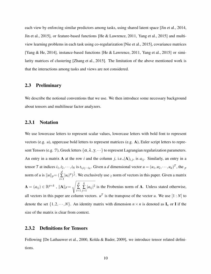
2.3 Preliminary

We describe the notional conventions that we use. We then introduce some necessary background

about tensors and multilinear factor analyzers.

2.3.1 Notation

We use lowercase letters to represent scalar values, lowercase letters with bold font to represent

vectors (e.g. u), uppercase bold letters to represent matrices (e.g. A), Euler script letters to repre-

sent Tensors (e.g. T), Greek letters α,λ ,γ, · · · to represent Lagrangian regularization parameters.

An entry in a matrix A at the row i and the column j, i.e.,(A)i, j, is ai j. Similarly, an entry in a

tensor T at indices i1, i2, · · · , iN is ti1i2···iN . Given a d dimensional vector u = (u1,u2, · · · ,ud)T , the p

norm of u is ‖u‖p= (d∑

i=1|ui|p)

1p . We exclusively use 2 norm of vectors in this paper. Given a matrix

A = (ai j) ∈ Rp×k , ‖A‖F=

√p∑

i=1

k∑j=1|ai j|2 is the Frobenius norm of A. Unless stated otherwise,

all vectors in this paper are column vectors. uT is the transpose of the vector u. We use [1 : N] to

denote the set 1,2, · · · ,N. An identity matrix with dimension n× n is denoted as In or I if the

size of the matrix is clear from context.

2.3.2 Definitions for Tensors

Following [De Lathauwer et al., 2000, Kolda & Bader, 2009], we introduce tensor related defini-

tions.

10

Definition 1 (Tensor Order). The order of a tensor is the number of its dimensions. Given an

Nth-order tensor T ∈ RI1×I2×···×IN with N indices, each index addressing a mode of T.

Example 1. We use the tensor A ∈ R2×3×2 where I1 = 2, I2 = 3, I3 = 2 through out this paper for

illustration purposes. In this example A is specified as

A:,:,1 =

1 1 0

2 1 3

,A:,:,2 =

2 1 2

1 1 0

,

where A:,:,1 is the matrix found in the tensor A by fixing the last index and varying other indices.

Clearly the order of A is 3.

Definition 2 (n-mode Fibers). Fibers are generalization of row/column vectors of a tensor. A

n-mode tensor fiber of a tensor T is any vector obtained in T by fixing all but the nth index of T.

Example 2. For a 2nd-order tensor ( i.e., a matrix), the 1-mode fibers are its columns and the

2-mode fibers are its rows.

In Fig. 2.1, we illustrate the three n-mode fibers of A, where n = 1,2,3. Each 1-mode fiber of

A is a vector of length I1 = 2 and there are a total of I2× I3 = 3×2 = 6 1-mode fibers in A. Those

fibers are: 1

2

,

2

1

,

1

1

,

1

1

,

0

3

,

2

0

.

By convention 1-mode fibers are called column fibers, 2-mode fibers are row fibers, and 3-mode

fibers are tube fibers. For a tensor T with order 3, we use t(:, j,k) to denotes its column fibers, t(i,:,k)

for its row fibers, t(i, j,:) for its tube fibers.

Definition 3 (n-mode Product). Given an Nth-order tensor T ∈RI1×I2×···×IN and a vector v∈R1×In ,

the n-mode tensor-vector product (1 ≤ n ≤ N) between T and v is a tensor of order N-1, denoted

by

11

2X3X2I1

I2

I3

II

III IV

I

Figure 2.1: Illustration of n-mode fibers. I: a tensor A ∈ R2×3×2, II:1-mode (column) fibers, III:2-mode (row) fibers, IV:3-mode (tube) fibers.

T×n v ∈ RI1×I2×···×In−1×In+1×···×IN , and the entries of the new tensor are given by

(T×n v)i1i2···in−1in+1···iN = ∑in

ti1i2···in−1inin+1···iN vin. (2.1)

Example 3. Let v = [1 2 1], the 2-mode tensor vector product between A and v is a matrix where

elements are the inner products between the row-fibers of A and v, or

A×2 v =

va(1,:,1) va(1,:,2)

va(2,:,1) va(2,:,2)

=

3 6

7 3

Throughout this paper we only use tensor vector multiplication and hence we do not attempt to

define tensor matrix multiplication.

Tensor matricization is a widely used operation to “unfold” a tensor into a matrix, as defined

below.

Definition 4 (n-mode Matricization). Given a tensor T, the n-mode matricization, denoted as

T(n) ∈ RIn×(In+1In+2···IN I1I2···In−1), is the matrix T(n) whose columns are the n-mode fibers of T.

Example 4. For the tensor A, it has three n-mode matricization, where n = 1,2,3. Its 1-mode

12

matricization is A(1) of size RI1×(I2I3), where I1 = 2, I2I3 = 3×2 = 6.

A(1) =

(a(:,1,1) a(:,1,2) a(:,2,1) a(:,2,2) a(:,3,1) a(:,3,2)

)

=

1 2 1 1 0 2

2 1 1 1 3 0

.

2.3.3 Probabilistic Multilinear Factor Analyzers (MLFA)

Extending from classical factor analyzer (FA), which use one latent variable, bilinear models

[Tenenbaum & Freeman, 2000] consider the situation where observations are modulated by two

latent variables. Multilinear factor analyzers (MLFA) [Tang et al., 2013] are further generalization

of bilinear models so that they model multiplicative interactions of N different latent variables,

corresponding to N groups of factors. Given an observed vector x ∈ RP, N latent variables as

z1,z2 · · ·zN where zi ∈RIi , a factor loading tensor D∈RP×I1×I2×···×IN with order N+1, a generative

model for x can be conveniently formulated by the tensor vector multiplication as:

x =D×2 z1×3 z2 · · ·×N+1 zN + ε (2.2)

where ε is an i.i.d error term following a multinomial Gaussian distribution. With the error term ε ,

one may apply maximum likelihood estimation or Bayesian to estimate model parameters such as

zs and/or D for different learning tasks.

Before we start to connect probabilistic MLFA to MTVL learning, we show two variations

of (2.2). These variations are obtained by straightforward algebraic operations but are useful in

extending the calculation to MVTL learning and in deriving efficient optimization techniques.

13

Proposition 1. With the same set up of (2.2), we have

D×2 z1×3 z2 · · ·×N+1 zN

=D(1)(z1⊗ z2⊗ . . .⊗ zN) (2.3)

= ∑(i1,i2,···,iN)

(N

∏k=1

zk,ik)d:,i1,···,iN (2.4)

where D(1) is the 1-mode matricization of the loading tensor D, ⊗ is the Kronecker product

operator, d:,i1,···,iN is a column fiber (1-mode fiber) of D. zk,ik is the ikth element of the vector zk.

The significance of (2.3) is that it shows tensor vector multiplication has an equivalent matrix

vector multiplication format. We use this property to derive efficient optimization techniques in

the next section. (2.4) shows that the same calculation can be viewed as a linear span of 1-mode

fibers of the tensor D where the weight are provided by (multiplicative) interactions of the vectors.

We use this formula to extend MLFA to generate vectors with different lengths.

The proof of the propositions is a straightforward application of definitions that we provide

before. Readers may check the appendix A for expanded details of proofs that we omit in this

section and the next section.

2.4 Algorithm

In this section, we first formally define the MTVL learning problem. We then develop a new multi-

linear factor analysis algorithm, adaptive-basis multilinear factor analyzers (aptMLFA). Based on

aptMLFA, We propose an algorithm aptMTVL for MTVL learning to disentangle task-view-label

interactions. We also develop a variation of our own method without considering interactions for

the comparison with aptMTVL.

14

Table 2.1: Notations for MTVL Learning Problem

T Total number of tasksV Total number of viewsL Total number of labels

Xt,v Object-feature matrix of the labeled trainingdata for the task t in the view v

Yt,v Object-label matrix of the training data forthe task t in the view v

Xt,vu Object-feature matrix of the unlabeled training

data for the task t in the view vVt The set of views present in the task tTv The set of tasks having the view v

2.4.1 Problem Formulation

Suppose we have data from T tasks, V views. The label space of the data is denoted as L =

l1, l2, · · · , lL with L possible labels. For each task t ∈ [1 : T ] from view v ∈ [1 : V ], we have labeled

training data (Xt,v,Yt,v) and unlabeled training data Xt,vu . Xt,v ∈RNt×Pv

is the object-feature matrix

for the labeled training data. Yt,v ∈ 0,1Nt×L is the binary object-label matrices for the labeled

training set where each row corresponds to a sample and each column is a label for the sample.

The entry of Yt,v at the ith row and jth column is 1 if the sample i is annotated with the label l j

and 0 otherwise. Nt is the total number of labeled training samples for the task t. In addition, we

denote the set of views present in task t as Vt ,|Vt |≤V .

We assume that each sample of task t has the same number of views, i.e., if a view is present

in one sample in a task, it is present in every sample in this task. The set of tasks having the view

v is denoted as Tv, where |Tv|≤ T .

We summarize some important notations used for our problem in Table 6.1.

2.4.2 MTVL Learning with Task-View-Label Interactions

The goal of our algorithm is to learn a predictor f t,v,l for each task t from view v associated with

label l. For simplicity we assume the function is linear and is parameterized by a vector θt,v,l . Our

hypothesis is that those vector θt,v,l are modulated simultaneously by three types of factors, tasks,

15

views and labels, naming as task factor, view factor and label factor respectively. These 3 types of

factors influence each other on the predictors. A learning model that is capable of accommodating

the interactions between these different types of factors should achieve better performance. To

this end, we treat θt,v,l as “observed data" in MLFA; and use three latent variables to represent

task, view and label respectively. However, multilinear factor analyzers cannot be directly applied

to MTVL learning problem because the vectors generated by MLFA must have the same length.

However in our case the length of the model parameters may be different for different views.

Therefore, those θt,v,ls cannot share the same factor loading tensor. To handle this, we develop a

flexible multilinear factor analyzers, adaptive-basis multilinear factor analyzers, where each group

of factors can affect the basis vectors in some way.

2.4.2.1 Adaptive-basis Multilinear Factor Analyzers (aptMLFA)

In adaptive-basis multilinear factor analyzers, we expect that each factor may have its own loading

tensor. To avoid having too many parameters, some information must be shared among those

loading tensors. To this end, our idea is to introduce another type of latent variables for each

group of factors so that each factor may modulate the factor loading tensor. Specifically, given N

groups of factors, for the nth group, there are Jn factors. We denote the jnth factor in this group as

zn, jn , where zn, jn ∈ RIn,n ∈ [1 : N]. For each factor zn, jn , we introduce another latent factor Un, jn ,

which corresponds to a transformation matrix. Let D∈RP×I1×I2×···×IN be the factor loading tensor.

Then we use the following generative model for the observed data x modulated by latent vectors

z1, j1,z2, j2 , · · · ,zN, jN as

x j1, j2,···, jN

=∑(z1, j1i1 U1, j1)(z2, j2

i2 U2, j2) · · ·(zN, jNiN UN, jN )d:,i1,i2,···,iN + ε (2.5)

16

where the summation is across all tuples (i1, i2, · · · , iN). d:,i1,i2,···,iN are 1-mode fibers of D. Note

that the dimensions of Un, jn’s need to be compatible. Different from the preliminary section, we

use superscripts rather than subscripts for vector z. The notation change makes sense since we

are adapting MLFA to MTVL learning where we will soon use superscripts for tasks, views, and

labels.

In classical MLFA, each observed data x can be seen as a point in a I1×I2×·· ·×IN-dimensional

space. Each dimension of that space represents a prototype of data identified by a basis vector,

which is a 1-mode fiber of the loading tensor D. The coordinates of x in this space are determined

by the N latent factors. Note that the dimension of each basis vector must be the same since all

latent factors share the same loading tensor. Therefore, MLFA cannot be used to model data with

different dimensions.

Different from MLFA, aptMLFA avoids the vector length limitation by enabling each factor

to use a specific loading tensor, which may be different from the loading tensors used by other

factors. At the same time, those factor-specific loading tensors are related to each other through

a basic loading tensor D. The interpretation of aptMLFA is that each observed data x can be in a

different I1× I2×·· ·× IN-dimensional space. Those spaces are transformations of the basic space

formed by the 1-mode fibers of D. Those transformations are realized through modifying basis

vectors of prototypes. In other words, (2.5) suggests that to generate x we simultaneously take two

considerations: (i) the linear span of 1-mode fibers of a loading tensor where the weights are pro-

vided by multiplication of components in zs, and (ii) the transformation itself is the multiplication

of transformations associated with each z.

With AptMLFA we are ready to present our design of the MTVL learning algorithm that are

capable of disentangling interactions of tasks, views, and labels. In this set up we have three factor

groups: tasks, views, and labels, and hence N = 3. For each group we have multiple factors. For

example for the task group we have multiple tasks and each task is described by a latent vector z.

Associated with latent vector is a transformation matrix U and all of the latent vectors share the

same loading tensor (of order 4). Below we present the algorithm to “learn” those latent vectors,

17

transformation matrices, and the order 4 loading tensors in an efficient approach.

2.4.2.2 MTVL Learning using aptMLFA (aptMTVL)

In this section, we give the details of using adaptive-basis multilinear factor analyzers to design

MTVL learning. For simplicity, we formulate our algorithm using linear function as the prediction

function f t,v,l . The objective function J of aptMTVL consists of four components, as denoted

below:

J = O +C +I +R (2.6)

The first term in (2.6) is the squared loss for labeled training samples and we have:

O =T

∑t=1

|Vt |

∑v=1‖Yt,v−Xt,v

Θt,v‖2

F

The second term is employed to achieve view consistency using co-regularization technique

[Sindhwani et al., 2005] by penalizing the difference among the prediction results on unlabeled

samples from different views of the same task t. To be specific,

C = α

T

∑t=1

|Vt |

∑v,v′=1‖Xt,v

u Θt,v−Xt,v′

u Θt,v′‖2

F (2.7)

here α ∈ R is a parameter for controlling the weight of this term in the objective function.

The third term is used to model the task-view-label interactions. To be specific, each θt,v,l is

modeled as interactions of three groups of factors, task factors, view factors and label factors. Let

pt ∈ Rm denote the task factor of task t, qv ∈ Rn the view factor of view v and sl ∈ Rk the label

factor for label l. For task factors and label factors, we assume that they do not change the factor

loading tensor. That is, the transformation matrices for task factors and label factors are identity

matrices I. That is, Ut = IPv and Ul = IP. For view factor qv, we denote the transformation matrix

18

as Uv ∈ RPv×P. Let D ∈ RP×m×n×k be the factor loading tensor, then θt,v,l can be formulated as

θt,v,l = ∑

i, j,h(pt

iUt)(qv

jUv)(sl

hUl)d:,i, j,h

= ∑i, j,h

(ptiIPv)(q

vjU

v)(slhIP)d:,i, j,h

= ∑i, j,h

ptiq

vjs

lhUvd:,i, j,h (2.8)

For convenience, we represent this formulation in a more concise but equal form,

θt,v,l = Wv

(1)(pt⊗qv⊗ sl), (2.9)

where Wv(1) = UvD(1). Wv

(1) is the 1-mode matricization of the transformed loading tensor Wv ∈

RPv×m×n×k for the view v and D(1) is the 1-mode matricization of the basic loading tensor D. The

equivalence of (2.8) and (2.9) follows from proposition (4).

To sum, applying aptMLFA we introduce a view specific loading tensor Wv. To avoid leaning

too many parameters we require that all the view specific loading tensors are transformations of a

common base loading tensor. Mathematically we specify the third term in (2.6) as:

I =β

T

∑t=1

|Vt |

∑v=1

L

∑l=1‖θ t,v,l−Wv

(1)(pt⊗qv⊗ sl)‖22+

γ

V

∑v=1‖Wv

(1)−UvD(1)‖2F (2.10)

The last term in (2.6) regularizes the complexity of predictor parameters using norms of pa-

19

rameters and hence avoids overfitting. It is:

R =λ

V

∑v=1‖Uv‖2

F+µ‖D(1)‖2F+

η

T

∑t=1‖pt‖2

2+ζ

V

∑v=1‖qv‖2

2+

ρ

L

∑v=1‖sl‖2

2 (2.11)

By utilizing multilinear factor analyzers, we provide a principled framework to design machine

learning algorithms entangling interactions of many factors. Our model can be easily applied to

multi-task multi-view learning, multi-view multi-label learning, and multi-task multi-label learn-

ing. When there are new types of relationship need to be considered, our model can be easily

extended to incorporate the new relationship by introducing a new group of factors. In addition

missing data including missing views and missing labels can also be addressed in aptMTVL by

only regulating the interactions between existing labels in a task and a view. More over transfer

learning can be realized for missing views or missing labels. To be specific, for missing views in

a task, view factor qv learned from other tasks can be leveraged to estimate θ . Similarly, a label

factor sl learned from other tasks can be used for a task with missing labels. Rather than extending

those points in the subsequence study we focus on the approach that we use to efficiently learn

those parameters.

We denote all the model parameters as

Ω = (θ t,v,l,Wv(1),U

v, pt ,qv,sl,D(1)),

∀ t ∈ [1 : T ],v ∈ [1 : V ], l ∈ [1 : L]

then our aim is to solve the optimization problem:

argminΩ

J (2.12)

20

2.4.2.3 Optimization for aptMTVL

For optimization, we use an alternating method to solve θt,v,l,Wv

(1),Uv, pt ,qv,sl,D(1) iteratively. In

each iteration, we identify the optimal value for a parameter by fixing the rest parameters. To do so

we compute the gradient of the corresponding objective function and we show that we have close

form solution. The non-trivial part in gradient calculation is to identify optimal values for pt ,qv,sl

because of the Kronecker product. For that we derive a set of propositions to assist the calculation.

Our strategy is to first convert Wv(1)(pt ⊗ qv⊗ sl) into an equivalent tensor multiplication form

W×2 (pt)T ×3 (qv)T ×4 (sl)T (Proposition 4) and then calculate the derivative of W×2 (pt)T ×3

(qv)T ×4 (sl)T using a general and simple formula (Proposition 5).

Proposition 2. Given the tensor T ∈RI1×I2×···×IN and the vectors x2 ∈R1×I2, x3 ∈R1×I3, · · · , xN ∈

R1×IN , one has

∂ (T×2 x2×3 x3 · · ·×N xN)

∂ (xk)T =

(T×2 x2 · · ·×k−1 xk−1×k+1 xk+1 · · ·×N xN)T (2.13)

Rather than proving the proposition we provide an example to illustrate the calculation.

Example 5. Given a tensor A, which is a matrix A∈RI1×I2 , and a vector x∈RI2 , we have A×2 x∈

RI1 according to Def. 3 and the entries of A×2 x are given by

(A×2 x)i1 =I2

∑i2=1

ai1i2xi2

It is obvious that AxT ∈ RI1 and

(AxT )i1 =I2

∑i2=1

ai1i2xi2

Thus, we have A×2 x = AxT and ∂ (A×2x)∂xT = ∂ (AxT )

∂xT = AT .

21

Below we provide the results of our calculation. The proof of the proposition (5) and the

details derivation process of the optimization are documented in the Appendix section of this paper,

available online.

θt,v,l =((Xt,v)T Xt,v +α(|Vt |−1)(Xt,v

u )T Xt,vu +β IPv)−1

((Xt,v)T yt,v +α

|Vt |

∑v′ 6=v,v′=1

(Xt,vu )T Xt,v′

u θt,v′,l)+

βWv(1)(pt⊗qv⊗ sl)) (2.14)

pt = (βCp +ηIm)−1

β

|Vt |

∑v=1

L

∑l=1

(Av,lp )T

θt,v,l (2.15)

Where Av,lp =W×3 (qv)T×4 (sl)T ∈RPv×m. The c-th column of Cp is

|Vt |∑

v=1

L∑

l=1

n∑

i=1

k∑j=1

b:,(c−1)nk+(i−1)k+ jqvi sl

j,

where b’s are columns of Bv,lp = (Av,l

p )T Wv(1)

qv = (βCq +ζ In)−1

β

|Tv|

∑t=1

L

∑l=1

(At,lq )T

θt,v,l (2.16)

Where At,lq =W×2 (pt)T×4 (sl)T ∈RPv×n. The c-th column of Cq is

|Tv|∑

t=1

L∑

l=1

n∑

i=1

k∑j=1

b:,(i−1)nk+(c−1)k+ j ptis

lj,

where b’s are columns of Bt,lq = (At,l

q )T Wv(1)

sl = (βCs +ηIk)−1

β

T

∑t=1

V

∑v=1

(At,vs )T

θt,v,l (2.17)

Where At,vs =W×2 (pt)T×3 (qv)T ∈RPv×k. The c-th column of Cs is

T∑

t=1

V∑

v=1

n∑

i=1

k∑j=1

b:,(i−1)nk+( j−1)k+c ptiq

vj,

where b’s are columns of Bt,vs = (At,v

s )T Wv(1)

22

Wv(1) =(β

|Tv|

∑t=1

θt,v(pt⊗qv⊗ sl)T + γUvD(1))

(β|Tv|

∑t=1

(pt⊗qv⊗ sl)(pt⊗qv⊗ sl)T + γImnk)−1 (2.18)

Uv = γWv(1)D

T(1)(γD(1)DT

(1)+λ IP)−1 (2.19)

D(1) = (γV

∑v=1

((Uv)T Uv +µIP)−1

γ

V

∑v=1

((Uv)T Wv(1)) (2.20)

We summarize our algorithm in Algorithm 1.

2.4.3 MTVL Learning without Interactions

(aptMTVL−)

To demonstrate the effect of modeling task-view-label interactions, we propose a base-line method

without considering the interactions. The objective functions of this base-line method is also com-

posed of four components:

J − = O +C +I −+R− (2.21)

The first term and the second term are the same as the corresponding terms in (2.6). For the third

term, we replace pt⊗qv⊗ sl with rt,v,l so that the interactions are not formulated. Thus we denote

23

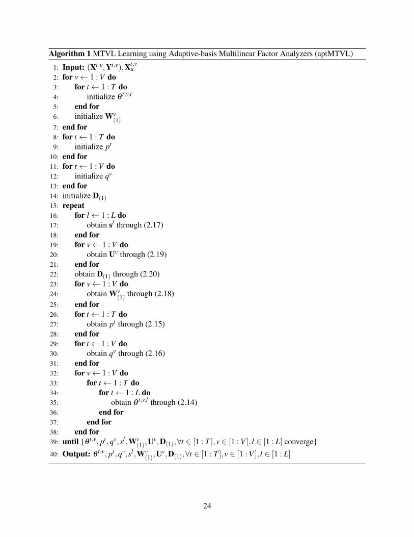
Algorithm 1 MTVL Learning using Adaptive-basis Multilinear Factor Analyzers (aptMTVL)

1: Input: (Xt,v,Yt,v),Xt,vu

2: for v← 1 : V do3: for t← 1 : T do4: initialize θ

t,v,l

5: end for6: initialize Wv

(1)7: end for8: for t← 1 : T do9: initialize pt

10: end for11: for t← 1 : V do12: initialize qv

13: end for14: initialize D(1)15: repeat16: for l← 1 : L do17: obtain sl through (2.17)18: end for19: for v← 1 : V do20: obtain Uv through (2.19)21: end for22: obtain D(1) through (2.20)23: for v← 1 : V do24: obtain Wv

(1) through (2.18)25: end for26: for t← 1 : T do27: obtain pt through (2.15)28: end for29: for t← 1 : V do30: obtain qv through (2.16)31: end for32: for v← 1 : V do33: for t← 1 : T do34: for t← 1 : L do35: obtain θ

t,v,l through (2.14)36: end for37: end for38: end for39: until θ

t,v, pt ,qv,sl,Wv(1),U

v,D(1),∀t ∈ [1 : T ],v ∈ [1 : V ], l ∈ [1 : L] converge

40: Output: θt,v, pt ,qv,sl,Wv

(1),Uv,D(1),∀t ∈ [1 : T ],v ∈ [1 : V ], l ∈ [1 : L]

24

it as:

I − =β

T

∑t=1

|Vt |

∑v=1

L

∑l=1‖θ t,v,l−Wvrt,v,l‖2

2+

γ

V

∑v=1‖Wv−UvD‖2

F (2.22)

and modify the regularization term correspondingly:

R− =λ

V

∑v=1‖Uv‖2

F+µ‖D‖2F+

η

T

∑t=1

V

∑v=1

L

∑l=1‖rt,v,l‖2

2 (2.23)

This formulation can be seen as an extension of the latent space based approach proposed in

[Kumar & Daumé III, 2012] for multi-task learning to MTVL learning using the strategy pro-

posed in previous MTMV learning methods [Yang & He, 2014, Zhang & Huan, 2012]. That is, we

decompose MTVL learning into V multi-task multi-label learning problems with one multi-task

multi-label learning problem in each view. To capture the inter-task and inter-label relationship in

view v, we assume that each θ t,v,l,∀t ∈ Tv,∀l ∈ L, can be factorized into two factors, a latent basis

Wv and a vector rt,v,l , where Wv ∈ RPv×k, rt,v,l ∈ Rk. Wv is shared among all tasks in v and rt,v,l

is task, view and label specific. In addition, to handle the inter-view relationship, we assume latent

bases Wvs for different views are linear transformations of a underlying latent space, denoted as

D ∈ RP×k. We denote the transformation matrix for view v as Uv ∈ RPv×P.

Using the similar method for optimizing (2.6), we can get closed form solution for θt,v,l,rt,v,l,Wv,Uv,D,∀t ∈

25

[1 : T ],v ∈ [1 : V ] at each step of iteration:

θt,v,l =((Xt,v)T Xt,v +α(|Vt |−1)(Xt,v

u )T Xt,vu +β IPv×Pv)−1

((Xt,v)T yt,v,l +α

|Vt |

∑v′ 6=v,v′=1

(Xt,vu )T Xt,v′

u θt,v′,l)+

βWvrt,v,l) (2.24)

rt,v,l = (β (Wv)T Wv +ηI)−1β (Wv)T

θt,v,l (2.25)

Wv =(β|Tv|

∑t=1

L

∑l=1

θt,v,l(rt,v,l)T + γUvD)

(β|Tv|

∑t=1

L

∑l=1

rt,v,l(rt,v,l)T + γIk)−1 (2.26)

Uv = γWvDT (γDDT +λ IP)−1 (2.27)

D = (γV

∑v=1

((Uv)T Uv +µIP)−1

γ

V

∑v=1

((Uv)T Wv) (2.28)

We summarize aptMTMV− in Algorithm 2.

2.5 Experimental Studies

We implemented the proposed aptMTVL learning algorithm using Matlab. We conducted several

experiments to evaluate the classification accuracy of aptMTVL learning using multiple real-world

data sets. We compared our algorithm with HiMLS since it is the only existing work on MTVL

learning and its effectiveness has been demonstrated in [Yang & He, 2015] in comparing with other

26

Algorithm 2 MTVL Learning without task-view-label Interactions (aptMTVL−)

1: Input: (Xt,v,Y t,v,l),Xt,vu

2: for v← 1 : V do3: for t← 1 : T do4: initialize θ

t,v,l

5: end for6: initialize Wv

7: end for8: initialize D9: repeat

10: for v← 1 : V do11: for t← 1 : T do12: for l← 1 : L do13: obtain rt,v,l through (2.25)14: end for15: end for16: end for17: for v← 1 : V do18: obtain Uv through (2.27)19: end for20: obtain D through (2.28)21: for v← 1 : V do22: obtain Wv through (2.26)23: end for24: for v← 1 : V do25: for t← 1 : T do26: for l← 1 : L do27: obtain θ

t,v,l through (2.24)28: end for29: end for30: end for31: until θ

t,v,l,rt,v,l,Wv,Uv,D,∀t ∈ [1 : T ],v ∈ [1 : V ] converge32: Output: θ

t,v,l,rt,v,l,Wv,Uv,D,∀t ∈ [1 : T ],v ∈ [1 : V ]

multi-label or multi-view multi-label learning algorithms. We obtained the matlab sources code

of HiMLS from the original developing teams. In order to further evaluate the effectiveness of

aptMTVL we also implemented the aptMTVL− algorithm which does not handle the interactions

with tasks, views, and labels.

In the following, we first describe the data sets and our experimental protocol. We then present

the experimental results and a brief discussion.

27

2.5.1 Data Sets

The three data sets used in experiments are described as follows.

Enron Data Set. This data set [Alcalá et al., ] contains 1,702 email messages labeled using 53

labels that forms a hierarchy of two levels. Bag-of-words is used for features and the number of

features for each message is 1001. We used 33 leaf labels for our experiments by excluding those

leaf labels with less than 50 messages. Each label in the top level is considered as a task. Thus

we generate 3 tasks by using all the documents that belong to the corresponding first-level label

as training and test data. we applied two dimensionality reduction methods, ICA and PCA, to the

original features to generate 2 views.

Eurlex Data Set. This data set [Loza Mencíá & Fúrnkranz, 2010] is a collection of 19,348

documents about European Union law. The first most frequent 5,000 words are used to calculate

TF-IDF features for each document. All the documents are classified using 412 categories orga-

nized in a hierarchy of four levels. Leaf categories can be in any level of the hierarchy. We use

leaf categories with more than 100 documents as selected labels to get 65 labels. Each category

in the top level is treated as a task. Those first-level categories whose child nodes do not contain

any selected labels are excluded. We generate 17 tasks in total. For each label in each task, we

randomly select less than 200 documents to generate training and test data samples. Similar to

Enron data set, we also applied two dimensionality reduction methods to the original features to

generate 2 views.

Reuters Corpus Data Set. Reuters Corpus data set [Lewis et al., 2004] contains 80,4414 doc-

uments classified using 101 hierarchical categories. We constructed the data for our experiments

using a subset of this data set using the following process. We generate 9 tasks from 13 second-

level categories that do not correspond to assignable categories by selecting those categories that

contain at least 2 child categories and in whose documents at least 50 assignable categories present.

We selected those leaf categories that present in each task and contains at least 40 documents to

generate 11 labels. For each task and each label, we randomly selected 100 documents to generate

training and test data samples. Two views are generated by applying PCA to features generated

28

using TF-IDF and bag-of-words.

For clarity, we summarize the characteristics for each data set in Table 2.2.

Table 2.2: Training Size and Test Size.T is the total number of tasks. V is the total number ofviews. Pi is the number of features in each view i, i ∈ 1,2. N is the total number samples foreach task.

Data Set T V P1 P2 NEnron 3 2 371 514 3,841Eurlex 17 2 1,360 1,800 11,724

Reuters 9 2 3,205 3,205 9,699

2.5.2 Experimental Protocol

In this section, we explain the procedure we used for model selection and the metrics used for

performance evaluation

Model Selection. For each algorithm, we randomly select 80% of the samples from each task

for training and the rest for test.

We tuned all the parameters of aptMTVL and other baseline methods using 5-fold cross val-

idation on the training data set. In this approach 80% of the training data was used for building

a model, the rest was used for validation. After the optimal parameters were found, final mod-

els were trained using all the training data. Then we applied final models to the test data to get

experimental results.

We repeated our training, model selection, and model evaluation process for 10 times. We

report the average the performance on the testing data sets.

Model Evaluation Metrics. We use both F1 and the area under the ROC curve (AUC) to

compare performance of algorithms. F1 is defined as follows,

F1 =1L

L

∑l=1

2×T Pl

2×T Pl +FPl +FNl

Where T Pl,FPl,FNl are true positives, false positives, false negatives for the lth label respec-

tively. We then calculate the average F1 score across all labels. In literature this is known as the

29

Enron Eurlex Reuters

0.05

0.1

0.15

0.2

0.25

0.3

0.35

0.4

0.45

0.5

F1

aptMTVL

aptMTVL−

Enron Eurlex Reuters

0.65

0.7

0.75

0.8

0.85

0.9

0.95

1

AU

C

aptMTVL

aptMTVL−

Figure 2.2: Performance Comparison w/o Task-view-label Interactions

macro-F1 score.

AUC is calculated as the average AUC for each label using

AUC =1L

L

∑l=1

AUCl

Where AUCl is calculated for the lth label. In literature this is known as the macro AUC.

2.5.3 Experimental Results and Discussion

To test our hypothesis that handling interactions of tasks, views, and labels is the key factor for

the success of multi-task, multi-view, multi-label learning, we compare our proposed algorithm

aptMTVL with the base line method,

aptMTVL−, where interactions are not modeled. We then present the results of performance com-

parison between

aptMTVL and HiMLS.

Performance Comparison Between aptMTVL and aptMTVL−. In Fig. 2.2 we show

the comparison results between aptMTVL and its variation, aptMTVL−. We see that aptMTVL

achieved better performance than aptMTVL− on all three data sets. On Enron data set, the perfor-

mance of aptMTVL− is close to aptMTVL. The reason of this may be that the relatedness between

leaf categories that belong to different parent categories are weak.

Performance Comparison Between aptMTVL and HiMLS.2 We present the performance

2It is worth noting that we use subsets of Eurlex and Reuters different from those used in [Yang & He, 2015] for

30

Table 2.3: Performance Comparison of Algorithms

AUC F1Data Set HiMLS aptMTVL HiMLS aptMTVL

Enron 0.570 0.652 0.054 0.187Eurlex 0.909 0.957 0.009 0.086

Reuters 0.517 0.810 0.056 0.476

comparison of between aptMTVL and HiMLS in Table 2.3. From the results we see that aptMTVL

consistently outperforms HiMLS on all three data sets on AUC and F1 scores. Note that HiMLS

has a very low macroF1 score on Eurlex. To uncover the possible reason, we examined the predic-

tion results of HiMLS and found that the results were predicted according to majority vote. That

is, the predicted labels for all the samples are the same as the true label that had majority number

of samples. For the Reuters Corpus data set we notice that the object-feature matrices of reuters

corpus data set is very sparse, in which about 98% entries are zero. This may pose a challenge

for learning relationship among data through matrix factorization, which is the technique used by

HiMLS. From the testing results aptMTVL tolerates sparse matrices well.

2.6 Conclusion

We studied MTVL learning that involving complex relationship modulated by three types of fac-

tors, task factors, view factors and label factors. To tackle the complex relationship, we developed

an adaptive basis multilinear factor analyzers and applied it to MTVL learning. The flexibility

of aptMTVL enables our algorithm to be easily adapted to other machine learning problems with

relationship affected by more than one factor, such as MTV, MTL and MVL learning. In addition,

our algorithm can also be extended to incorporate new kinds of relationships by simply introduc-

ing new factors. We compared our proposed algorithm with the state-of-the-art MTVL learning

algorithm using three real-world data sets and demonstrated the effectiveness of the algorithm.

our experiments. In addition, random splitting instead of a specific splitting of training and test is performed in ourexperiments.

31

Chapter 3

Multilinear Dirichlet Processes

3.1 Introduction

Dependent Dirichlet processes (DDP) have been widely applied to model data from distribu-

tions over collections of measures which are correlated in some way. To introduce dependency

into DDP, various techniques have been developed via correlating through components of atomic

measures, such as atom sizes [Griffin & Steel, 2006, Rodriguez & Dunson, 2011] and atom lo-

cations [De Iorio et al., 2004, Gelfand et al., 2005], sampling from a DP with random distribu-

tions as atoms [Rodriguez et al., 2008], operating on underlying compound Poisson processes

[Lin et al., 2010], regulating by Lévy Copulas [Leisen et al., 2013], or constructing those mea-

sures through a mixture of several independent measures drawn from DPs [Hatjispyros et al., 2016,

Kolossiatis et al., 2013, Ma et al., 2015].

On the other hand, in recent years, increasing research efforts in machine learning and data min-

ing have been dedicated to dealing with heterogeneously related data involving interactions from

two or more factors. For example, in multilinear multi-task learning [Romera-Paredes et al., 2013],

predictions of a student’s achievement may be affected by both her school environment and time.

In context aware recommender systems, different conceptual factors, such as time and companions,

play major roles on a user’s preferences for restaurants.

However, few researchers have addressed the heterogeneous relationship in data brought by

modulation of multiple factors using techniques of DDP. To the best of our knowledge, the only

work that considered multiple groups of factors was proposed by De Iorio et al. [De Iorio et al., 2009,

De Iorio et al., 2004]. In their work, the dependence in collections of related data was introduced

32

by building an ANOVA structure across atom locations of random measures. The main weak-

ness of ANOVA based DDP is that the model becomes cumbersome when the number of factors

increases and the inference may be computationally daunting, especially when the multiplicative

interactions of factors are also included in the ANOVA effects. In addition, the method assumes

that the effects of a factor are the same for those samples which are affected by that factor. How-

ever, this assumption may be invalid in some situations. For example, the school environment may

have varying degrees of impact in the academic performance of each student.

In this work, we propose a novel technique of constructing DDP based on DP and multilinear

factor analyzers (MLFA) [Tang et al., 2013] to overcome the limitations in aforementioned studies.

We refer to this method as Multilinear Dirichlet Processes (MLDP). Specifically, we are trying to

model S sets of samples that are correlated through N groups of factors by constructing S dependent

random measures, with one random measure used to model the distribution of one set of samples.

To capture the correlations among different sets of samples, we hypothesize that those S dependent

random measures are the results of multiplicative interactions of N groups of factors. Specifically,

we represent each random measure as a linear combination of I different latent basis measures. We

may consider each basis measure as a 1-mode fiber of a shared latent factor tensor in MLFA. Then

we determine the weights of those linear combinations using multiplicative interactions of latent

parameter vectors that correspond to different factor groups by borrowing the ideas from MLFA.

To evaluate the performance of MLDP, we have compared it with DP-based methods using

3 synthetic data sets and 4 real world data sets. In addition, we have applied MLDP to various

machine learning problems, multilinear multi-task learning, and context-aware recommendation,

which have received much attention from researchers recently. The comprehensive experiments

demonstrate the effectiveness of MLDP on different applications.

The contribution of this work is two-fold:

• We have developed a novel technique MLDP to construct DDPs by combine DP with multi-

liear factor analyzers to model the distributions of data modulated by different factors.

• We have demonstrated the effectiveness of MLDP by applying it to density estimation and

33

two real world applications, multilinear multi-task learning and context-aware recommender

systems and evaluating MLDP on 4 real-word data sets. The state-of-the-art performance

achieved by MLDP has validated its applicability to those applications.

3.2 Related Work

Dependent Dirichlet Processes has long standing in the literature of Bayesian nonparametric meth-

ods. A wide variety of techniques have been developed to address various correlations of sets

of samples. The interested reader is referred to a comprehensive survey conducted by Foti and

Williamson [Foti & Williamson, 2015]. Those techniques can be categorized into two groups

according to the heterogeneity of underlying factors which a method aims to capture for un-

tangling the correlations. Most of existing techniques of DDP, which belong to the first group,

only consider one underlying factor which leads to the correlations among samples, such as space

[Gelfand et al., 2005], time [Caron et al., 2007], study [Muller et al., 2004], or pairwise distance

[Blei & Frazier, 2011].

For the methods in the second group, multiple groups of factors were taken into account

when modeling correlations. Compared with the considerably large number of previous works

in the first group, few studies have been dedicated to capturing multiple factors. De Iorio et al.

[De Iorio et al., 2004] proposed a method to model dependence across related random measures

by building an ANOVA dependence structure among atom locations of random measures. In a

later work, De Iorio et al. [De Iorio et al., 2009] further proposed a linear DDP model by ex-

tending the ANOVA DDP model to include continuous covariates through a DP mixture of linear

models.

3.3 Preliminary

In this section, we introduce necessary background knowledge about tensors and Multilinear Factor

Analyzers on which our method is based.

34

3.3.1 Notations

For clarity, we introduce the notations that will be used throughout the paper. We use lowercase

letters to represent scalar values, lowercase letters with bold font to represent vectors (e.g. u),

uppercase bold letters to represent matrices (e.g. A), and Euler script letters to represent Tensors

(e.g. T). Unless stated otherwise, all vectors in this paper are column vectors. We use [1 : N] to

denote the set 1,2, . . . ,N.

3.3.2 Basic definitions for Tensors

Following [De Lathauwer et al., 2000, Kolda & Bader, 2009], we introduce some basic definitions

for tensors.

Definition 5 (Order). The order of a tensor is defined as the number of dimensions of a tensor. A

Nth-order tensor, denoted as A ∈ RI1×I2×···×In , has N indices with each index addressing a mode

of A.

Definition 6 (n-mode Fiber). Fibers are defined as vectors that constitute a tensor. A n-mode tensor

fiber is obtained by varying the nth index of the tensor while fixing all other indices. Columns and

rows are 1-mode and 2-mode fibers for a matrix, i.e. a 2nd-order tensor, respectively.

3.3.3 Multilinear Factor Analyzers

As an extension of bilinear models [Tenenbaum & Freeman, 2000], which was originally devel-

oped to untangle “content" and “style" factors in images, Multilinear factor analyzers (MLFA)

[Tang et al., 2013] were developed to model data that is the result of multiplicative interactions of

N groups of factors, with Jn factors in each group. Let denote the jnth factor in factor group n

using a latent parameter vector zn, jn , where j ∈ [1 : Jn], zn, jn ∈ RIn , and n ∈ [1 : N], then MLFA

formulate an observed vector x j1,..., jN ∈ RP modulated by factors j1, . . . , jN using a shared latent

35

factor tensor D ∈ RP×I1×I2×...×IN as follows [Li & Huan, 2016]:

x j1,..., jN = ∑i1,...,iN

(N

∏n=1

zn, jnin )d:,i1,...,iN + ε (3.1)

where d:,i1,...,iN is a 1-mode fiber of D. zn, jnin is the inth element of the vector zn, jn . ε is an i.i.d error

term following a multivariate Normal distribution.

3.4 Algorithm

In this section, we first formulate the problem we aim to solve. Then we describe the details of

the proposed method multilienar Dirichlet Processes (MLDP). Lastly, we present the inference

algorithm we have developed for MLDP.


Given N groups of factors, and Jn observed factors in the nth group , we collect a set of samples,

X j1,..., jN ∈ RM j1,..., jN×P, for each combination of factors from N groups, where one factor is used

for each group, to get S = J1×J2 . . .JN sets of samples in total. Here jn is used to specify that jnth

factor in group n is used in the combination. For example, suppose there are 2 groups of factors

with 2 factors in each group, i.e. J1 = J2 = 2, then we have S = J1× J2 = 4 sets of samples X1,1,

X2,1, X1,2, X2,2, where X1,2 is affected by two factors, 1st factor in factor group 1 and 2nd factor

in factor group 2.

Our goal is to fit S sets of samples using generative models based on DDP techniques. Note

that those S sets of samples are modulated by the interactions of N groups of factors. Therefore, to

better fit the data, a model that can capture the interactions among different factors is needed. To

this end, we propose Multilinear Dirichlet Processes by borrowing ideas of modeling interactions

among factors from Mulitlinear factor analyzers (MLFA). Note that MLFA were designed for fac-

tor analysis of observed samples represented in vectors. It cannot be directly applied to modeling

distributions. To leverage the advantage of MLFA for tackling multiplicative interactions of fac-

36

Table 3.1: Notations for MLDP

N Total number of factor groupsJn Total number of factors in the nth

factor groupS Total number of sets of samples

X j1,..., jN The set of samples modulated byfactors j1, . . . , jN

In Total number of basis measures forthe nth factor group

G∗i1,...,iN The basis measure indexed by(i1, . . . , iN)

G j1,..., jN The random measure used to modelX j1,..., jN

un, jn The latent parameter vector for jnthfactor in factor group n

w j1,..., jNi1,...,iN The linear combination weight

of G∗i1,...,iN for G j1,..., jN

tors, we equate a group of basis random measures with the shared latent factor tensor D in MLFA,

treating each basis measure as a 1-mode fiber of D. Then a random measure can be constructed

using a linear combination of those basis random measures by determining the weights of linear

combinations using the same technique in MLFA. However, there is another challenge posed by

employing MLFA for model random distribution. In MLFA, the weights of linear combinations

can be any real numbers. In order to construct a valid random measure, the weights of a linear com-

bination must be positive and sum to one. To this end, we utilize a softmax function to normalize

the weights.

Before proceeding to the formulation of MLDP, we summarize important notations for MLDP

in Table 3.1.

3.4.2 Multilinear Dirichlet Processes

Given N groups of factors, we assume that each factor in a factor group corresponds to a latent

parameter vector u ∈ RIn . Then we use linear combinations of I = I1× I2 . . . IN basis measures G∗

37

to define Multilinear Dirichlet Processes (MLDP) as follows:

G j1,..., jN = ∑i1,...,iN

w j1,..., jNi1,...,iN G∗i1,...,iN

G∗i1,...,iN ∼ DP(α,H)

f or jn ∈ [1 : Jn], in ∈ [1 : In],n ∈ [1 : N] (3.2)

G∗i1,...,iN is represented using the form:

G∗i1,...,iN =∞

∑k=1

πki1,...,iN δ

φ ki1,...,iN

where the weights πki1,...,iN can be iteratively constructed using a stick-breaking process with pa-

rameter α [Sethuraman, 1994]. And each atom φ ki1,...,iN is an i.i.d draw from the base distribution

H.

The weights for the linear combinations of basis measures G∗’s are determined by latent pa-

rameter vectors u’s through softmax functions:

w j1,..., jNi1,...,iN =

eu1, j1i1

u2, j2i2

...uN, jNiN

∑k1,k2,...,kN

eu1, j1k1

u1, j2k2

...uN, jNkN

un, jnin ∼ N(0,(σn

u )2) log((σn

u )2)∼ N(0,σ2

0 )

f or in ∈ [1 : In], jn ∈ [1 : Jn],n ∈ [1 : N]

where un, jn = [un, jn1 , . . . ,un, jn

In]T is a latent parameter vector for jnth factor in factor group n. un, jn

in is

the inth element of un, jn . Note that w j1,..., jNi1,...,iN has the property that ∑

i1,...,iNw j1,..., jN

i1,...,iN = 1.

Properties of MLDP. Let denote all the latent parameter vectors u’s as U, then it is apparent

38

that for any Borel set B, we have:

EG j1,..., jN (B)|U

= ∑i1,...,iN

w j1,..., jNi1,...,iN H(B) = H(B) (3.3)

VG j1,..., jN (B)|U

= ∑i1,...,iN

(w j1,..., jNi1,...,iN )2

1+αH(B)(1−H(B)) (3.4)

From the above properties of MLDP, we can see that the expectation of each random distribution,

G j1,..., jN (B), which corresponds to a combination of factors from N groups, is the same given U.

And the difference in variance of G j1,..., jN (B) is determined by ∑i1,...,iN

(w j1,..., jNi1,...,iN )2.

It is worth noting that DP is a special case of MLDP when the dimensions of u’s are 1.

w j1,..., jN1,1,...,1 =

eu1, j11 u2, j2

1 ...uN, jN1

eu1, j11 u1, j2

1 ...uN, jN1

= 1

G j1,..., jN = w j1,..., jN1,1,...,1 G∗1,1,...,1 = G∗

f or jn ∈ [1 : Jn],n ∈ [1 : N]

From the above derivation, we can see that here is only one basis measure when the dimensions of

u’s are 1 and this basis measure is a draw from a DP. That is, G j1,..., jN is a draw from a classical

DP and a MLDP degenerates to a DP.

In the above definition of MLDP (3.2), we assume that basis measures are drawn from the same

DP(α,H) to allow rather limited heterogeneity in data. On the other end of the spectrum of the

heterogeneity, we may use DP’s with different parameters for G∗s to have:

G∗i1,...,iN ∼ DP(αi1,...,iN ,Hi1,...,iN )

f or in ∈ [1 : In],n ∈ [1 : N] (3.5)

39

G∗i1,...,iN can be represented using the form:

G∗i1,...,iN =∞

∑k=1

πki1,...,iN δ

φ ki1,...,iN

Similarly, the weights πki1,...,iN can be iteratively constructed using a stick-breaking process with

parameter αi1,...,iN . And each atom φ ki1,...,iN is an i.i.d draw from base distribution Hi1,...,iN .

Although the high flexibility of MLDP allows it to model extremely heterogeneous data, this

may entail the issue of unidentifiability. To address this issue, we may add constraints to those

factor loadings u’s or induce sparsity into MLDP. Specially, we may consider using sparsity-

promotion priors, such as a hierarchical Student-t prior [Tipping, 2001] or a spike-and-slab prior

[Ishwaran & Rao, 2005], to allow a small set of basis measures are used and improve identifiability.

We defer this topic to future work.

3.4.3 MLDP Mixture of Models

Having defined MLDP, the mixture of models using MLDP is straightforward. Given a set of

samples, X j1,..., jN ∈ RM j1,..., jN×P, for each combination of factors from N groups, where there are

Jn factors in the nth factor group. We use the following generative model for X’s

x j1,..., jNm ∼ f (·|θ j1,..., jN

m )

θj1,..., jN

m ∼ G j1,..., jN

G j1,..., jN ∼MLDP

f or m ∈ [1 : M j1,..., jN ], jn ∈ [1 : Jn],n ∈ [1 : N]

where x j1,..., jNm ∈ R1×P is the mth row of X j1,..., jN .

40

3.4.4 Computation

We use approximate inference based on Markov Chain Monte Carlo (MCMC) methods for MLDP

since the inference cannot be obtained analytically. Specifically, we use a Gibbs sampler to approx-

imate the posterior distribution of model parameters (φ ki1,...,iN ,u

n, jn,σnu ) by extending Algorithm 8

proposed in [Neal, 2000] since it does not require fixed truncation and can handle non-conjugate

base measures by using auxiliary clusters.

There are two main challenges in inference of MLDP. First, a mixture of multiple basis mea-

sures is used in MLDP. Secondly, the weights of the mixture are determined by groups of factors

in a multilinear way. For the first challenge, we introduce additional indicator variables b j1,..., jNm to

specify which basis measure is used for a sample. To be specific, we have b j1,..., jNm = (i1, . . . , iN)

if and only if the corresponding basis measure for x j1,..., jNm is G∗i1,...,iN . For the second challenge,

that is, the posterior approximation of w j1,..., jNi1,...,iN , we have developed a method based on Hamiltonian

dynamics [Neal et al., 2011] to update un, jn since w are deterministic given u.

In the following, we give the detailed process of computing model parameters (φ ki1,...,iN ,u

n, jn ,σnu )

in each iteration of MCMC. We first describe the steps of assigning a sample to a basis measure

and a cluster of that basis measure. Then we present the formulations used for updating model

parameters.

Update cluster and basis measure assignments. The major difference between the inference

of MLDP and that of classical DP is that we also need to determine which basis measure, i.e. G∗, is

used for a specific sample in addition to cluster assignment decisions. To tackle this, We introduce

additional indicator variables b j1,..., jNm to indicate which basis measure is used for a sample. To be

specific, we have b j1,..., jNm = (i1, . . . , iN) if and only if the corresponding basis measure for x j1,..., jN

m

is G∗i1,...,iN . In addition, similar to the inference in classical DP, we also introduce a latent indicator

variable c j1,..., jNm , which specify the cluster a sample x j1,..., jN

m belongs to, to facilitate the inference.

We use the following procedure in each iteration to update b j1,..., jNm , c j1,..., jN

m , for m ∈ [1 : M j1,..., jN ],

jn ∈ [1 : Jn], n ∈ [1 : N].

41

First let define:

ρki1,...,iN =

rw j1,..., jN

i1,...,iNl−m,ki1,...,iN

L−mi1,...,iN

+αf (x j1,..., jN

m |φ ki1,...,iN )

f or k = 1, . . . ,K−mi1,...,iN

rw j1,..., jN

i1,...,iNα/s

L−mi1,...,iN

+αf (x j1,..., jN

m |φ ki1,...,iN )

f or k = K−mi1,...,iN +1, . . . ,K−m

i1,...,iN + s

here r is the appropriate normalizing constant; s is the number of auxiliary clusters; K−mi1,...,iN is the

number of active clusters in basis measure G∗i1,...,iN ; L−mi1,...,iN is the total number of samples assigned

to the basis measure G∗i1,...,iN ; and l−m,ki1,...,iN is the number of samples that are allocated to cluster k.

Note that we use the superscript −m to denote that the sample x j1,..., jNm is excluded. φ k

i1,...,iN ’s are

drawn from the base distribution of G∗i1,...,iN when K−mi1,...,iN +1≤ k ≤ K−m

i1,...,iN + s.

Then we generate a draw (b j1,..., jNm , c j1,..., jN

m ) based on the following probability:

(b j1,..., jNm = i1, . . . , iN ,c j1,..., jN

m = k |Ω)

= ρki1,...,iN (3.6)

where Ω = (x j1,..., jNm ,U,B−m,C−m,Φ). We use U to denote all the latent vectors un, jn’s. B−m and

C−m are used to denote sets of indicator variables b j1,..., jNm ’s and c j1,..., jN

m ’s respectively without

considering x j1,..., jNm . And Φ is the set of φ k

i1,...,iN ’s.

Update U. To update U, we use the Hamiltonian dynamics method [Neal et al., 2011]. A non-

trivial step in applying Hamiltonian dynamics is to compute the derivative of log probability of B

w.r.t. U. To tackle this, we first encode the value of b j1,..., jNm using a vector z j1,..., jN

m ∈ RI1×I2×···×IN ,

where the i1, . . . , iN th element of z j1,..., jNm is 1 if b j1,..., jN

m = i1, . . . , iN . For the following derivation,

we use z by omitting the superscript and subscript of z j1,..., jNm for clarity.

42

According to MLDP, the probability of b j1,..., jNm given U can be written as:

p(b j1,..., jNm = i1, . . . , iN |U)

=eu1, j1

i1u2, j2

i2...uN, jN

iN

∑k1,k2,...,kN

eu1, j1k1

u2, j2k2

...uN, jNkN

=e(u

1, j1⊗u2, j2 ...⊗uN, jN )T×z

∑k1,k2,...,kN

eu1, j1k1

u1, j2k2

...uN, jNkN

Then the log probability of all b’s which are determined by un, jnin has the following form:

L = log ∏J−n

M j1,..., jN

∏m=1

p(b j1,..., jNm )

= ∑J−n

(M j1,..., jN

∑m=1

(u1, j1⊗u2, j2 . . .⊗uN, jN )T × z−

M j1,..., jN log ∑k1,k2,...,kN

eu1, j1k1

u2, j2k2

...uN, jNkN )

The derivative of L w.r.t un, jnin is calculated using:

∂L

∂un, jnin

= ∑J−n

(M j1,..., jN

∑m=1

(u1, j1⊗ . . .

un−1, jn−1⊗un+1, jn+1 . . .⊗uN, jN )T × z−

∑K−n

u1, j1k1

. . .uN, jNkN

eα) (3.7)

43

where

α =u1, j1k1

. . .uN, jNkN

un, jnin −

log ∑k1,k2,...,kN

eu1, j1k1

u1, j2k2

...uN, jNkN ,

J−n = j1, . . . , jn−1, jn+1, . . . , jN,

I−n =i1, . . . , in−1, in+1, . . . , iN,

K−n =k1, . . . ,kn−1,kn+1, . . . , iN,

and z only contains elements of z which will multiply un, jnin in u1, j1⊗u2, j2 . . .⊗uN, jN .

After having derived ∂L/∂un, jnin , the updating of U is straightforward. The interested user is

referred to [Neal et al., 2011] for details.

Update Σu. Given un, jn , for jn ∈ [1 : Jn], n∈ [1 : N], we can sample σnu from the posterior using:

p(σnu |·) ∝

Jn

∏jn=1

In

∏in=1

p(un, jnin |σ

nu )p(σn

u ) (3.8)

Update Φ. To reduce clutter, we abbreviate the subscript and superscript of x j1,..., jNm as g =

[m,( j1, . . . , jN)] and denote x j1,..., jNm as xg. Let use G k

i1,...,iN to denote the set of g’s of x’s which

belong to cluster k of basis measure G∗i1,...,iN . Then we draw a new value for φ ki1,...,iN according to

the following probability:

p(φ ki1,...,iN |·) ∝ ∏

g∈G ki1,...,iN

f (xg|φ ki1,...,iN )H(φ k

i1,...,iN ) (3.9)


In this section, we evaluate the performance of MLDP by applying it to density estimation and two

real world applications: multilinear multi-task learning (MLMTL), and context-aware recommen-

dation system (CARS) using 3 synthetic data sets and 4 real-world data sets. For each data set, we

44

randomly selected r% of samples as training data set and used all the rest as test data set, where

r = 10,20, . . . ,80 for experiments of density estimation and r = 50 for experiments of MLMTL and

CARS. We repeated this process 10 times for each data set and reported the averaged performance

on the test data set. We select the hyperparameters through 10-fold cross validation. For MCMC,

we ran for 5,000 iterations with a burn in period of 3,000. The inference did converge according to

our examination of the parameters for each cluster. We computed the final results by following the

method used in [Shahbaba & Neal, 2009]. Specially, 2,000 post-convergence samples simulated

from MCMC were used to estimate posterior predictive probabilities.

3.5.1 Density Estimation

To study the performance of MLDP on estimating the density of heterogeneous data that is mod-

ulated by different groups of factors, we generate 3 synthetic data sets according to our MLDP

model, except the number of components in each basis measure is fixed to 2. The statistics of these

data sets are summarized in Table 3.2. We use Normal Gamma distribution NG(µ0,λ0,κ1,κ2) as

the base distribution for each basis measure. For the parameters, we have µ0 = 100∗ i, λ0 = 0.01,

κ1 = 2 ∗ i, κ2 = 0.01, and σ0u = 1, where i ∈ [1 : 2×Nb] and Nb is the number of total basis

measures.

For the comparison methods, we use DP, and two DDP methods, a mixture of Dirichlet Pro-

cesses (MXDP) proposed in [Muller et al., 2004], and ANOVA-based dependent Dirichlet pro-

cesses (ANOVADP) [De Iorio et al., 2004].

The results are presented in Fig. 3.1. We observe that MXDP, ANOVADP, and MLDP outper-

forms DP on both SDS1 and SDS2, which demonstrates the effectiveness of DDP-based methods

on borrowing strength across sets of samples. On all 3 data sets, MLDP achieves best performance,

showing a clear advantage over the other 3 methods. This strengthens our conviction that MLDP

can better model heterogeneous data modulated by different factors.

45

Data Set N Jn In Nb NcSDS1 2 2 2 4 8SDS2 2 2 3 9 18SDS3 3 2 2 8 16

Table 3.2: Statistics of Synthetic Data Sets. N: Number of Factor Groups. Jn: Number of factorsin nth group. In: Dimension of latent parameter vectors for nth group. Nb: Number of BasisMeasures. Nc: Number of Total Components (Nb×2)

0 0.2 0.4 0.6 0.8−6.5

−6

−5.5

−5

−4.5

−4

−3.5

−3

avg log p

robabili

ty

DP

MXDP

ANOVADP

MLDP

0 0.2 0.4 0.6 0.8−7.5

−7

−6.5

−6

−5.5

−5

−4.5

−4

avg log p

robabili

ty

DP

MXDP

ANOVADP

MLDP

0 0.2 0.4 0.6 0.8−7.5

−7

−6.5

−6

−5.5

−5

−4.5

−4

−3.5

avg log p

robabili

ty

DP

MXDP

ANOVADP

MLDP

Figure 3.1: Form Left to Right: 1. SDS1; 2. SDS2; 3.SDS3.

a b c d e g0.5

1

1.5

2

2.5

3

RM

SE

a b c d e g10

12

14

16

18

20

RM

SE

a b c f g200

250

300

350

400

450

500

550

RM

SE

a b c f g0.6

0.65

0.7

0.75

AU

C

Figure 3.2: Form Left to Right: 1. MLMTL on Restaurant & Consumer Data set; 2. MLMTLon School Data set; 3. CARS on Frappe Data Set; 4. CARS on Japan Restaurant Data Set.Algorithms: a. DP-MRM; b: MXDP-MRM; c: ANOVADP-MRM; d: MLMTL-C; e:TPG; f:CSLIM; g:MLDP-MRM

46

3.5.2 Multilinear Multi-task Learning (MLMTL)

In multilinear multi-task learning (MLMTL), each task is associated with two or multiple modes.

For example, in predicting ratings given by a specific consumer to different aspects of a restaurant,

such as food quality or service quality, a MLMTL algorithm formulates the problem by considering

each combination of one consumer and one aspect (two modes) as a task using a 2-dimensional

indexing.

To handle MTMTL, we use MLDP Mixture of Regression Models (MLDP-MRM) by treating

each mode as a factor group. Suppose there is a set of tasks associated with N modes with Jn aspects

in the nth mode. For a task indexed by ( j1, . . . , jN), we obtain a set of samples (X j1,..., jN ,y j1,..., jN ),

where X j1,..., jN ∈ RM j1,..., jN×P and y j1,..., jN ∈ RM j1,..., jN . The following MLDP-MRM model is used

in our experiments:

x j1,..., jNm ∼ N(µ j1,..., jN

x,m ,Σ j1,..., jNx,m )

y j1,..., jNm ∼ N(x j1,..., jN

m βj1,..., jNm ,σ j1,..., jN

y,m )

(µ j1,..., jNm ,Σ j1,..., jN

x,m ,β j1,..., jNm ,σ j1,..., jN

y,m )∼ G j1,..., jN

G j1,..., jN ∼MLDP

f or m ∈ [1 : M j1,..., jN ], jn ∈ [1 : Jn],n ∈ [1 : N]

We use generative regression models to model the distributions of both x and y since they have

been widely used for DP-based mixture models and their effectiveness has been demonstrated in

previous work [Wade et al., 2014, Shahbaba & Neal, 2009]. But note that it is not the limitation of

MLDP and other types of regression models can also be used with MLDP, for example, we may

only model the distribution of y given x.

47

For computationally convenient, we use the following priors for basis distribution H

H(µx,Σx,β ,σy) =NIW(µx,Σx; µ0x ,λ0,Ψ

0x ,ν0)

N(β ;0,σ2y V)IG(σ2

y ;ay,by) (3.10)

We compared MLDP-MRM with 3 other Mixture of Generative Regression Models, DP-MRM,

MXDP-MRM and ANOVADP-MRM, using different mixing measure, DP, MXDP [Muller et al., 2004],

and ANOVADP [De Iorio et al., 2004] respectively. In addition, we also used two state-of-the-art

MLMTL algorithms, MLMTL-C [Romera-Paredes et al., 2013], which is based on convex tensor

trace norm regularization, and TPG [Yu & Liu, 2016], which is based on prototypical method of

projected gradient descent, for comparison. 2 real-world data sets, restaurant data set and school

data set, were utilized for the experiments, which we describe in the following.

Restaurant & Consumer Data Set. This data set contains 1161 ratings, including food rating,

service rating, and overall rating, from 131 consumers for 130 restaurants [Vargas-Govea et al., 2011].

The task is to predict a consumer’s rating for a restaurant given the attributes of the consumer and

the restaurant. We converted categorical attributes using binary coding to obtain 71 features for

each sample. Then we applied PCA to the training data set to keep the first 25 components and

then performed the same transformation on the test data set using the learned loadings. There are 2

groups of factors, corresponding to consumers and different aspects of the ratings. For the number

of factors, we have J1 = 131 and J2 = 3.

School Data Set. The school data set consists of examination records from 140 secondary

schools in years 1985,1986 and 1987. The attributes of the data include 4 school-specific at-

tributes and 3 student-specific attributes, where categorical attributes are expressed as binary fea-

tures [Argyriou et al., 2008]. The number of features used in the experiments were 19 after apply-

ing PCA. We organized the data according to 2 groups of factors, corresponding to schools and

years of examination. We excluded those schools which did not contain records from all 3 years to

obtain 64 schools. Thus we have J1 = 64 and J2 = 3. The prediction goal is to estimate a student’s

48

examination score.

Root mean squared error (RMSE) was employed to evaluate the results. The performance of

different algorithms is showed in the first 2 sub-figures of Fig. 3.2. On the restaurant & con-

sumer data set, we observe that DDP-based methods, i.e. MXDP-MRM, ANOVADP-MRM, and

MLDP-MRM, outperforms DP-MRM with a large margin. Compared with MXDP-MRM and

ANOVADP-MRM, MLMTL-C, which is specially designed for MLMTL, has a clear advantage.

However, it is worth noting that our proposed method has achieved better performance than both

MLMTL and TPG. The results on school data set, showed in the 2nd sub-figure of Fig. 3.2,

present the similar trend except that ANOVADP-MRM performed worse than DP-MRM. This

demonstrated the applicability of MLDP to multilinear multi-task learning problems.

3.5.3 Context-aware Recommendation

In context-aware recommender systems, conceptual variables are also considered in making rec-

ommendations in addition to the attributes of users and items. In this experiment, we evaluate the

performance of rating predictions based on MLDP models. To apply MLDP to context-aware rec-

ommendation, we map each conceptual variable to a factor group and treat each context condition

as a factor.

Similar to the experiment for MLMTL, we used MLDP-MRM for prediction tasks and com-

pared it with DP-MRM, MXDP-MRM, and ANOVADP-MRM. Furthermore, we compared MLDP-

MRM with a context-aware recommender system, CSLIM [Zheng et al., 2014], to investigate whether

MLDP-MRM is competitive with the current state-of-the-art technique. Two real-world data sets,

Japan Restaurant Data set and Frappe Data set were utilized in the experiment. We describe them

in the following.

Frappe Data Set. This data set consists of usage history logs of 4082 context-aware mobile

apps from 957 users [Baltrunas et al., 2015]. There are 96203 entries in total. We randomly se-

lected 2000 entries for our experiment. For MLDP, we use 2 features, daytime and isweekend, as

2 factor groups, with J1 = 2 and J2 = 7, to organize the data. For CSLIM, we use all the features

49

as context parameters. The prediction goal is to estimate the number of times an app is used by a

user.

Japan Restaurant Data Set. It consists of 800 ratings from 8 users for 69 restaurants in Japan

[Oku et al., 2006]. There are 31 features in the data set. The prediction task for this data set is to

estimate a user’s rating for a restaurant given the restaurant attributes and context conditions. For

MLDP, we use 2 event parameters, holiday and relation, and users as 3 factor groups with J1 = 6,

J2 = 6 and J3 = 8. For CSLIM, we use all the features as context parameters.

We show the results of comparison using the last 2 sub-figures of Fig. 3.2. Similar to MLMTL,

RMSE was used for performance evaluation on Frappe data set. For this data set, we observed

large variance. The app usage count varies from 1 to about 20,00. For the results, we notice that

DP or DDP based methods outperforms the state-of-the-art context aware recommender method,

CSLIM. Among DP or DDP based methods, our proposed methods MLDP-MRM is significantly

better than other methods. It is worth pointing out that we conducted two studies use two different

definitions of MLDP, (3.2) and (3.5), due to the large variance in the data. We found that MLDP-

MRM achieved better performance when using (3.5) (In Fig. 3.2, we only show the results of

using (3.5)). This provides further evidence that MLDP has advantage in handling heterogeneous

data. For Japan restaurant data set, we used AUC since the labels are binary. On this data set,

CSLIM performed better than DP-MRM while the performance is worse than 3 other DDP based

methods, ANOVADP-MRM, MXDP-MRM and MLDP-MRM. Among those 3 methods, MXDP-

MRM performed consistently better.

3.5.4 Time Performance Evaluation

To evaluate the computation efficiency of MLDP, we conducted experiments using 4 real world

data sets on a machine with 3.5GHz CPU and 16GB memory. We reports the time (in seconds)

needed for each iteration in MCMC of ANOVADP and MLDP in table 3.3. From the results we

can see that the performance of ANOVADP decreases dramatically when the total number of fac-

tors increases, which confirms the weakness of ANOVADP in handling relatively large number of

50

Table 3.3: Time Performance Comparison in Seconds between ANOVADP and MLDP. J: num-ber of total factors;M: number of instances; A: ANOVADP with only additive effects; A+M:ANOVADP with both additive and multiplicative effects; ML: MLDP

J M A A+M MLRestaurant 134 1662 350 1330 15

School 67 4732 100 415 34Frappe 9 1000 6 22 4JapanR 20 400 33 489 2

factors. Compared with ANOVADP, the advantage of MLDP in computation efficiency is signifi-

cant. Especially for Restaurant & Consumer and JapanRestaurant data sets, it required two orders

of magnitude less time .

3.6 Conclusion

In this work, we have devised a novel DDP technique, MLDP, for tackling heterogeneous data

modulated by multiple groups of factors, which has been largely ignored in the field of DDP-based

methods. To demonstrate the effectiveness of our proposed method, we have applied MLDP to

different applications, multilinear multi-task learning, and context aware recommendations using

4 real-world data sets. Compared with other state-of-the-art methods, MLDP has achieved better or

competitive performance. This confirms the usefulness of MLDP as a way to handle data affected

by multiple factors.

51

Chapter 4

Lifelong Multi-task Multi-view Learing

4.1 Introduction

As a promising method to exploit information from multiple related tasks with multiple data

sources (a.k.a. views), Multi-task multi-view(MTMV) learning has begun to gain attention from

investigators in the data mining and machine learning communities [He & Lawrence, 2011, Jin et al., 2013,

Jin et al., 2014, Yang & He, 2014, Zhang & Huan, 2012]. MTMV learning aims to improve per-

formance of learning algorithms by leveraging relatedness from both tasks and views. To this

end, different MTMV methods have been proposed to model task and view relatedness simul-

taneously and have been applied to many application areas including web page classification

[He & Lawrence, 2011], image recognition and classification [Zhang & Huan, 2012], and spam

email filtering [Yang & He, 2014].

Differing from previously investigated MTMV learning topics, in this paper we study the prob-

lem of MTMV learning in a lifelong learning framework. Lifelong machine learning, like human

lifelong learning, learns multiple tasks over time [Silver et al., 2013]. Lifelong multi-task multi-

view (Lifelong MTMV) learning is a new data mining and machine learning problem where new

tasks and/or new views may come in anytime during the learning process.

To the best of our knowledge, there has been no previous effort dedicated to lifelong MTMV

learning. Our study of lifelong MTMV learning problem is motivated by many real-world appli-

cations. Examples are:

• In object recognition, MTMV learning has been utilized to improve prediction modeling by

leveraging the shared representation among different object categories (tasks) and different

52

types of features, such as shape, margin and texture. However, current MTMV learning

approaches do not consider the situation where learning systems may encounter objects from

new categories or new types of features.

• In user behavior prediction, investigators usually exploit similarity among different users

(tasks) for better modeling. In addition, the prevalence of social media sites like Facebook,

Twitter and LinkedIn provides the possibility to utilize information from multiple sources,

such as connections, blogs, and interest. How to deal with new users and/or information from

different sources of social media poses a challenge for current MTMV learning algorithms.

• Although MTMV learning has been successfully applied to spam email filtering [Yang & He, 2014],

how to adapt learned models to identify spam emails for new users (tasks) is still an issue.

Moreover, we may get new views, such as features about the sender’s domain. How to incor-

porate these new views into learning process at any time without modifications to existing

learning systems is also a problem.

To design efficient algorithms for lifelong MTMV we propose a latent space lifelong MTMV

(lslMTMV) learning method to exploit task relatedness and information from multiple views. In

this new method we map views to a shared latent space and then learn a decision function in the

latent space. Specifically, for each task and for each view in the task we learn a predictive model.

To handle view and task relationship we factorize the predictive model for a task t and a view

v into two components: a view specific mapping that maps the view v to a latent space and a

task specific decision function that maps from the latent space to the decision space. We further

hypothesize that the view specific mapping is shared among all tasks and the task specific mapping

is shared among all views. Our model has many advantages among which the most significant one

is that we could retain the learned knowledge from previous tasks or view and transfer it to a new

model easily when a new task w/o new views arrive. To meet the efficiency requirement of lifelong

learning when more and more data arrives, we develop an optimization algorithm with low time

complexity by employing techniques from recursive least squares (RLS) for dictionary learning

53

[Skretting & Engan, 2010] and stochastic gradient descent (SGD). We have evaluated our method

using 3 real-world data sets. The experimental study results demonstrate that the classification

accuracy of our algorithm is close or superior to state-of-the-art offline MTMV learning algorithms

while the time needed to training such models is orders of magnitude less.

The main contributions of this work are three-fold:

• We are the first to study the MTML learning problem in an lifelong learning setting.

• We propose a latent space based MTMV learning algorithm (lslMTMV) to model relatedness

between tasks and views.

• We adapt our MTMV learning method to an lifelong learning setting by utilizing RLS and

SGD, allowing for efficiently coping with both new views and new tasks using learned

knowledge while refining it over time.

4.2 Related Work

Our work is related to two lines of research, MTMV learning and lifelong learning. We discuss

them separately in the following part.

MTMV Learning. To model task relatedness and view consistency, various techniques have

been developed by employing bipartite graph [He & Lawrence, 2011] or tree [Song et al., 2015],

regularization based method [Jin et al., 2013, Nie et al., 2015, Zhang & Huan, 2012], Bayesian non-

parametric [Yang & He, 2014], or LDA [Jin et al., 2014]. In addition to supervised learning, MTMV

learning has also been used for clustering [Zhang et al., 2015] by using bipartite graph co-clustering.

It is worth noting that all the previous works in MTMV learning are designed for the situation

where the training data are collected before the learning starts. One shortcoming of this offline

strategy is that it cannot efficiently deal with large training sets. In addition, they cannot handle

new tasks or new views.

Lifelong Learning. Lifelong learning is an active research area. It has been applied to super-

vised learning, semi-supervised learning, unsupervised learning and reinforcement learning. For

54

supervised learning, Silver et al. have proposed variants of sequential learning and consolidation

systems based on neural networks to address the problem of knowledge consolidation and the

stability-plasticity problem using task rehearsal [Fowler & Silver, 2011, Oquinn et al., 2005]. In

recent years, Lifelong learning has began to be applied to sentiment classification[Chen et al., 2015]

and opinion mining[Wang et al., 2016]. For semi-supervised learning, Mitchell & Cohen have de-

veloped Never-Ending Language Learner to cumulatively learning to read the web by acquiring

knowledge from the web 24 hours/day [Mitchell & Cohen, 2015]. For unsupervised learning, one

of the most recent work is [Le et al., 2012]. Le et al. have proposed a model, a deep autoencoder

with pooling and local contrast normalization using deep learning method, to build high-level fea-

tures for large-scale applications using only unlabeled data. Chen and Liu [Chen & Liu, 2014]

applied lifelong learning to topic modeling using topics from many domains. For reinforcement

learning, Ammar et al. recently developed a multi-task policy gradient method to learn decision

making tasks consecutively, transferring knowledge between tasks to accelerate learning.

Mostly related to our work, Ruvolo and Eaton [Ruvolo & Eaton, 2013c] developed an algo-

rithm to incorporate aspects of both transfer and multi-task learning using latent task structure

for lifelong learning. In an extended work [Ruvolo & Eaton, 2013a], they proposed to use active

task selection to boost performance in lifelong learning. None of the aforementioned algorithms

handles training data from multiple views.

In summary, although a considerable amount of research work has been carried out for lifelong

learning and MTMV learning separately. The investigation of the interplay of lifelong learning

and MTMV learning has just started and that is the focus of our paper.

4.3 Algorithm

4.3.1 Notations

We use the following notations throughout the rest of the paper. We use lowercase letters to rep-

resent scalar values, lowercase letters with bold font to represent vectors (e.g. u), uppercase bold

55

letters to represent matrices (e.g. A), Greek letters α,λ ,γ, · · · to represent regularization pa-

rameters. Given a p dimensional vector u = (u1,u2, . . . ,up)T , we define the Lq norm of u as

‖u‖q= (p∑

i=1|ui|q)

1q . Specially, we L2 norm of vectors in this paper. Given a matrix A= (ai, j)∈Rp×k

, ‖A‖F=

√p∑

i=1

k∑j=1|ai j|2 is the Frobenius norm of A. Unless stated otherwise, all vectors in this pa-

per are column vectors. uT is the transpose of the vector u.

We use superscripts to denote indices of views or tasks when we iterate over all the views or

tasks.


Suppose that we are given T tasks with features from V views. The number of features from some

view v ∈ 1,2, ...V is denoted as Pv. For some task t ∈ 1,2, ...,T , we are given Nt labeled and

Mt unlabeled training samples from |V t |≤ V views, where V t is a set containing views present in

task t. We assume that each batch data of task t has the same number of views, i.e., if a view

is present in one sample in a batch, it is present in every sample in this batch. For some view

v ∈V t present in the task t, we denote the training set from the view of the task t as (Xt,v,Ut,v,yt,v),

where Xt,v ∈ RNt×Pvis the object-feature matrix for the labeled training set, Ut,v ∈ RMt×Pv

is the

object-feature matrix for the unlabeled training set, and yt,v ∈RNtis the label vector for the labeled

training set. The set of tasks having the view v is denoted as T v, where |T v|≤ T . For example,

in Figure 4.1, we have T 1 = 1,2 for view 1, T 2 = 1,2 for view 2, T 3 = 1 for view 3, and

T 4 = 4 for view 4.

We summarize some important notations used for our problem in Table 4.1.

4.3.3 Latent Space MTMV Learning

Before we present our algorithm for the lifelong multi-task multi-view problem, we first present a

latent space based approach for the off-line multi-task multi-view (MTMV) learning problem. In

our method, for each view v of each task t, we first learn a prediction function f t,v(x) = f (x;θt,v),

56

View1 View2 View3 View4

Task1

Task2

Task1

Task3

Time

m0

m1

m2

m3

Figure 4.1: Lifelong Learning Problem

Table 4.1: Notations for the lifelong MTMV Learning Problem

T Total number of tasksV Total number of views

Xt,v Object-feature matrix of the labeled training data forthe task t in the view v

yt,v Labels of the training data for the task t in the view vUt,v Object-feature matrix of the unlabeled training data for

the task t in the view vLv The latent space shared by tasks from view vst The weight vector shared by all views in the task t

V t The set of views present in the task tT v The set of tasks having the view v

parameterized on θt,v ∈RPv

. We then make prediction by averaging the prediction results from all

views of task t. Instead of using training data only from the view v in the task t, we hope to learn a

better model for the task t by exploiting sharable knowledge from related tasks and multiple views.

To achieve this, we factorize θt,v into two latent factors, θ

t,v = Lvst , where Lv is a matrix factor

shared by all the tasks from the view v and st is a vector factor shared by all the views from the

task t. In essence, we characterize views using L and tasks using s. The interaction between Lv

and st captures the interaction between view v and task t. We assume that features of each task in

the same view v have similar contributions to that task so that they can share a latent space Lv.

We illustrate the factorization in a schematic plot in Figure 4.2. In this figure, θ1,1 and θ

2,1

share L1 since they are from the same view. θ1,1, θ

1,2 and θ1,3 share s1 since they are from

the same task. If the function f is a linear functional (which we focus in this paper) we have

57

f (x;θ t,v) = xT θ t,v = xT Lvst . We see that Lv maps the raw data to a latent space and st maps

from the latent space to a decision space. Following this interpretation, the matrix factorization is

interpreted as for a given view the mapping from the raw space to the latent space is shared among

all tasks (and hence Lv is task invariant). For a given task, different views are mapped to the shared

latent space and the final decision is made based on the information of the latent space (and hence

st is view invariant).

Task1

Task2

S

S

LL L

Ѳ1,1Ѳ1,2 Ѳ1,3

Ѳ2,1Ѳ2,2 Ѳ2,3

View1 View2 View3

1 2 3

L1 L2 L3

1

2

Figure 4.2: Latent Space MTMV Learning

Our latent space formalization for MTMV is novel and was never explored for MTMV prob-

lems. The advantages of this formalization, especially for lifelong learning with new tasks and new

views, are multifaceted. First, knowledge sharing among views is natural. All views are mapped to

the same latent space and the sharing of the knowledge gained from different views is very intuitive

and natural. Second, knowledge transfer among tasks can be easily achieved. When new tasks with

views that have seen before arrives (Case 2), knowledge learned from other tasks with same views

can be utilized to learn a better model for these tasks by sharing L. Similarly, when new views for

a task that has been studied before arrives (Case 3), the learned s can be used as a prior knowledge

so that there is no need to learn from scratch. Third, knowledge learned from new tasks or new

views can also be used to refine the model of tasks studied before since Lv is shared by all the tasks

in the same view v and st is shared across views for some task t. Moreover this formalization han-

dles missing views naturally. For tasks with missing (training) views, we are still able to use those

views if they are present in the test data set since we can use L of those missing views learned from

other tasks. We want to point out that our approach is a general form for the methods proposed

in [Kumar & Daumé III, 2012] and [Jia et al., 2010]. When there is only one view, our approach

58

degenerates to a latent space multi-task single view learning problem [Kumar & Daumé III, 2012].

When there is only one task, our method degenerates to a single task multi-view learning problem

[Jia et al., 2010], where we have the relationship: Lv = ((Dv)T Dv)−1(Dv)T . Note that the only

difference is that we use L2 norm instead of L1 norm for st .

Below we first give out details of the latent space MTMV learning algorithm and then we

present our strategy to adapt the algorithm for on-line and lifelong learning.

4.3.4 Latent Space MTMV Learning Details

We introduce our algorithm in an off-line setting here. For simplicity, we formulate our algorithm

using linear function as the prediction function f t,v. Our objective function is formalized as:

argminL,S

T

∑t=1

∑v∈V t

1Nt ‖y

t,v−Xt,vLvst‖22

+µ

T

∑t=1

∑v,u∈V t

v6=u

1Mt ‖U

t,vLv−Ut,uLu‖22

+λ

T

∑t=1‖st‖2

2+γ

V

∑v=1‖Lv‖2

F (4.1)

The first term in Equation 4.1 is the squared loss for labeled training samples. The second

term is used to achieve view consistency by penalizing the difference among prediction results

on unlabeled samples from different views of the same task t, where µ regulates the degree of

disagreement on different views. The parameter λ is used to control the complexity of st . The last

term regularizes the complexity of predictor parameters and hence avoids overfitting. The number

of latent bases is determined by parameter k, we use cross validation to obtain the optimal value of

k.

We use an alternating method to iteratively optimize Equation 4.1 between L and S since the

equation is not jointly convex but is convex with respect to L or S. For a fixed L, the optimization

59

function for a specific st is as follows:

argminst

∑v∈V t

1Nt ‖y

t,v−Xt,vLvst‖22+λ‖st‖2

2 (4.2)

To find the optimal Lv, we fix S and the rest of Lus (u ∈ 1,2, ...,V and u 6= v), and solve the

following optimization function:

argminLv

∑t∈T v

1Nt ‖y

t,v−Xt,vLvst‖22

+µ ∑t∈T v

∑u∈V t

v6=u

1Mt ‖U

t,vLv−Ut,uLu‖22+γ‖Lv‖2

F (4.3)

The calculation for st and Lv is straightforward. We can have closed-form solutions for st and

Lv by setting the derivative of (4.2) w.r.t. st and (4.3) w.r.t. Lv to zero. We omit the details due to

the space limit.

4.3.5 Latent Space Lifelong MTMV learning

In this section, we adapt our proposed method to an lifelong setting where training data are given

in mini-batches. Our goal is to design an lifelong MTMV learning algorithm that has lower com-

putational cost in terms of CPU time and memory space than the offline version. The basic ideas

are:

• We introduce intermediate variables θt,v so that batches of training data can be used itera-

tively to gradually update L . In addition, the complexity for optimization of S increases

with the total number of views instead of the amount of training data.

• We apply the optimization technique from Recursive Least Squares (RLS) [Skretting & Engan, 2010]

to continuously update θt,v.

• We utilize stochastic gradient descent (SGD) to gradually improve L.

60

• We partially update L, θt,v and S at each time stamp.

Objective function For Lifelong MTMV learning

For the offline algorithm, all training data needs to be stored in memory and used to update L and

S in each iteration since we try to exploit task relatedness and additional information from multiple

views. To deal with this inefficiency, we first introduce intermediate variables θt,v for each task t

from view v. We use m ∈ 1,2, . . . to index each time stamp when a batch of new training data

arrives. And we assume that the training data in each batch is from the same task. Then at each

time stamp m, we have the following objective function:

J =

T(1:m)

∑t=1

∑v∈V t

(1:m)

1Nt(1:m)

‖yt,v(1:m)−Xt,v

(1:m)θ

t,v‖22

+

T(1:m)

∑t=1

∑v∈V t

(1:m)

‖θ t,v−Lvst‖22

+µ

T(1:m)

∑t=1

∑v,u∈V t

(1:m)

v6=u

1Mt

(1:m)

‖Ut,v(1:m)

Lv−Ut,u(1:m)

Lu‖22

+λ

T(1:m)

∑t=1‖st‖2

2+γ

V(1:m)

∑v=1‖Lv‖2

F (4.4)

And our goal is to solve the following minimization problem:

argminL,S,Θ

J (4.5)

Where Θ = θt,v, ∀t ∈ 1,2, · · · ,T(1:m), v ∈ 1,2, · · · ,V(1:m). In the above Equation, we use sub-

script m to denote the value of a variable in time stamp m, (1 : m) to denote the cumulative values

of a variable from time stamp 1 to m. For examples, Xt,v(1:m)

denotes all the labeled training data

has been received until m, Xt,vm the labeled training data arriving at time stamp m, T(1:m) the total

number of seen tasks, V t(1:m) the set of seen views in task t.

61

To solve (4.4), if we directly apply alternating method used in offline learning to this objective

function, the complexity will increase dramatically with more and more data coming in because

all the received training data needs to be stored and used for optimization at each m. Suppose at

time stamp m, we receive a batch of data Xt,vm ∈RNm×Pv

,Ut,vm ∈RMm×Pv

and yt,vm ∈RNm ,∀v ∈V t

m, we

introduce different techniques for efficiently solving Θ, L and S in the following.

Optimization for Θ

The straightforward way to solve θt,v is to directly compute the following equation obtained y

setting the first derivative of (4.4) w.r.t θt,v to zero:

θt,vm = ((Xt,v

(1:m))T Xt,v

(1:m))−1(Xt,v

(1:m)yt,v(1:m)

+Lvmst

m) (4.6)

Note that in order to solve the above equation, we need to store and use all the received training data

until m. To tackle this inefficiency, we let At,vm = ((Xt,v

(1:m))T Xt,v

(1:m))−1 and Bt,v

m = (Xt,v(1:m)

yt,v(1:m)

+

Lvmst

m), and update At,vm and Bt,v

m iteratively as follows.

Updating At,vm Utilizing the techniques from RLS (Woodbury matrix identity), we can use the

following equation to update At,vm :

At,vm =At,v

m−1−

At,vm−1(X

t,vm )T ((Xt,v

m )At,vm−1(X

t,vm )T )−1(Xt,v

m )At,vm−1 (4.7)

By saving At,vm−1 and using it to sequentially update At,v

m , all the received training data does not

need to be stored and used at each time stamp.

Updating Bt,vm Similarly, we can sequentially update Bt,v

m by applying linear algebra to avoid

the cost of calculating using all the received data:

Bt,vm = Bt,v

m−1 +(Xt,vm )T yt,v

m +Ct,vm (4.8)

62

Where Ct,vm = αLv

mstm−αLv

m−1stm−1 is used to adjust the difference of Lv and st in previous step

and current step.

After updating At,vm and Bt,v

m , we can compute:

θt,vm = At,v

m Bt,vm (4.9)

Optimization for L

Assuming the received training data at m is composed of i.i.d samples from different views of a

task and utilizing stochastic gradient descent, we update Lvm as follows:

Lvm = Lv

m−1−ηm∇Jm(Lvm−1) (4.10)

Where ∇Jm(Lvm−1) is a gradient estimator of ∇J (Lv) using the batch of data at time stamp m:

∇Jm(Lvm−1) =

1Mt

m(αLv

m−1 ∑t∈T v

(1:m)

stm(s

tm)

T

+λ I+µ(|Vm−1|)(Xt,vm )T Xt,v

m Lvm−1

−α ∑t∈T v

(1:m)

θmt,v(sm

t)T

−µ ∑u∈V t

mu6=v

(Xt,vm )T Xt,u

m Lum−1) (4.11)

Where ηm is the gradient step at time stamp m.

In the above equation, the complexity of computing ∑t∈T v

(1:m)

stm(s

tm)

T and ∑t∈T v

(1:m)

θmt,v(sm

t)T in-

creases with the number of tasks. We may also alleviate this by letting Cvm = ∑

t∈T v(1:m)

stm(s

tm)

T and

63

Dvm = ∑

t∈T v(1:m)

θmt,v(sm

t)T and update Cvm and Dv

m iteratively to avoid summation over all tasks:

Cvm =Cv

m−1− stm−1(s

tm−1)

T + stm(s

tm)

T (4.12)

Dvm =Dv

m−1−θt,vm−1(s

tm−1)

T +θt,vm (st

m)T (4.13)

Note that the past information aggregated through stm and θ

t,vm can be used to improve Lv

m.

Optimization for S

By introducing Θ, the updating of st is relatively easy without incurring too much additional com-

puting complexity when new data arrives. Specially, by setting the derivative of (4.4) w.r.t st to

zero, we have:

stm =( ∑

v∈V t(1:m)

(Lvm−1)

T Lvm−1 + γI)−1

( ∑v∈V t

(1:m)

(Lvm−1)

Tθ

t,vm ) (4.14)

Partially Update L, S and Θ

Instead of updating each θt,v, Lv and st when new training data arrives, we only update θ

t,v, st of

task t to which new training data comes from and Lv of those views that present in task t due to the

reason that statistics information from previous training data can be accumulated through st and Lv

and transferred to tasks and views arriving later. Without significantly degrading the performance,

this method has been proved to be computationally efficient by our experiments on three real-world

data sets.

Algorithm 3 outlines the detailed steps for our approach.

64

Algorithm 3 Lifelong MTMV Learning using Latent Spaces

1: Input: µ,λ ,γ,α,k2: Initialize: T ← 0,V ← 03: for each m = 1,2, · · · do4: (Xnew,ynew,Unew, t,V t)← getNewData()5: if isNewTask(t)||isNewView(v) then6: Initialize θ

t,vm

7: end if8: if isNewView(v) then9: Initialize Lv

m10: end if11: Compute st

m using (4.14)12: for each v ∈V t do13: update At,v

m using (4.7)14: update Bt,v

m using (4.8)15: Compute θ

t,vm using (4.9)

16: end for17: for each v = 1 : V(1:m) do18: if viewHasTask(v, t) then19: update Cv

m and Dvm using (6.5)

20: end if21: end for22: for each v ∈V t do23: Compute ∇Jm(Lv

m−1) using (4.11)24: Update Lv

m using (4.10)25: end for26: save L: Lold ← L27: save S: Sold ← S28: end for29: Output: L,S,Θ

Analysis of Algorithm

Computational Complexity For simplicity, we assume the number of samples and the number of

views in each batch are the same. Then we give the time complexity for updating θt,v, st and Lv,

∀v ∈ V tm respectively, which are the three main steps in each iteration. For simplicity, we use P

as the maximum number of features in a view, omit subscript for the batch size Nm and the total

number of seen views V(1:m). For computing θt,v,∀v ∈ V t

m, the time complexity is O(|V tm|(NP2 +

PN2+N3+PN+PK)). Since we usually expect a small number of samples in each batch, then we

65

have PN. And we also assume P> k in general cases, thus the complexity will be dominated by

|V tm|NP2. For updating st , the time complexity is O(|V t

(1:m)|k2P+ |V t

(1:m)|kP+ k3), the complexity

will be dominated by |V tm|k2P since by utilizing the same assumption that P > k in general cases.

The time complexity for updating Lv,∀v ∈ V tm is O(|V t

m|(k2P+ |V tm|(NP2 + kP2))+V (k2 + kP)).

We can see that the major computational cost is from calculating |V tm|2kP2 +V kP. To sum, the

total complexity in each iteration is O(|V tm|NP2 + |V t

m|k2P+ |V tm|2kP2 +V kP) by only counting

the dominant terms of complexity. If we assume the number of views in each batch is small and

the total number of views V < P, the complexity can be further simplified to O(kP2). It is lower

than the complexity O(k2P3) of the multi-task single-view lifelong learning algorithm proposed in

[Ruvolo & Eaton, 2013c]. We also demonstrated the efficiency of our algorithm in the experiments

section.


We empirically evaluated the classification accuracy and the training time efficiency of our pro-

posed methods using multiple real-world and synthetic data sets. We have compared the offline ver-

sion of our methods lsMTMV to two state-of-the-art MTMV learning: the co-regularized MTMV

learning method CoRegMTMV [Zhang & Huan, 2012] and the MAMUDA method [Jin et al., 2014].

In addition, we compare (lslMTMV) with a lifelong multi-task single-view learning algorithm

ELLA. We could not compare with other algorithms in lifelong MTMV learning since we are the

first group to propose an algorithm for lifelong MTMV learning. To compare with ELLA, we

have concatenated features from all views to form a single view and used it as the training data for

ELLA.

Below we briefly review the data sets that we used and our experimental protocol. We then

present the results of the experimental study.

66

4.4.1 Datasets

We evaluate the performance of the proposed approach on the following three real-world data sets.

20 Newsgroups Data Set

The 20 Newsgroups data set consists of about 20,000 documents from 20 different newsgroups.

We generate TF-IDF for all the documents in each newsgroup. Then we applied dimensionality

reduction method PCA and ICA to generate 2 views for each document, with each view having

100 features. We treat each newsgroup as a task to form 20 tasks. The classification goal is to

determine whether each document belong to a newsgroup or not.

WebKB Data Set This data set contains a subset of the web pages collected from computer

science departments of 4 universities in January 1997 by the World Wide Knowledge Base (We-

bKb) project of the CMU text learning group [Rennie, 2007]. It is composed of 230 course pages

and 821 non-course pages. For each web page, two types of representation are provided, text on

the web page and anchor text of the hyperlinks to that page.

We treat each university as a task to form 4 tasks. Two views are created for each task using

TF-IDF. we generate the first view from text on the web pages and the second view from the

anchor text on the hyperlinks pointing to the corresponding pages. The classification goal here is

to determine whether a web page is a course page or not.

Diabetes Data Set The diabetes data set was collected from the Comparative Toxicogenomic

Database (CTD) [A.P. et al., 2016]. For our data set, we focussed on four diabetes diseases namely

Diabetes Mellitus, Diabetes Neuropathies, Diabetic Cardiomyopathies and Diabetes Angiopathies.

We treat each diabetes disease as a task to form 4 tasks and use 2d descriptors, gene and

pathway to form 3 views. For classification goal, we try to determine whether a drug interact with

a specific disease or not.

Synthetic Data Sets We generate multiple synthetic data sets to evaluate the training time

efficiency of different algorithms. To generate the data set, we first generate the shared matrix

factor Lv,∀v∈1,2, · · · ,V for each view and st ,∀t ∈1,2, · · · ,T for each task using the following

67

procedure:

µv i.i.d.∼ N (10,1)

σv i.i.d.∼ N (2,1)

Lv(i, j) i.i.d.∼ N (µv,(σ v)2),

∀i ∈ 1,2, · · · ,Pv, j ∈ 1,2, · · · ,k

st i.i.d.∼ N (0,Σs) (4.15)

Where N is Gaussian distribution, Σs is a diagonal matrix with 10 in the main diagonal. Then we

generate features in the first view using:

X t,1(i, j) i.i.d.∼ N (0,1),

∀i ∈ 1,2, · · · ,Nt, j ∈ 1,2, · · · ,Pv (4.16)

The features from other views are computed according to the following equation:

X t,v = X t,1L1(Lv)T (Lv(Lv)T +λ I)−1 (4.17)

Where I ∈ RPv×Pvis an identity matrix, λ = 1e−5.

We generate 3 groups of synthetic data sets. For the first group, we vary the number of features

in each view from 100 to 1000 incremented by 100 for 10 tasks from 2 views. For the second

group, we have incremented the number of tasks from 10 to 100 by 10 while keeping 2 views

and 500 features in each view fixed. To further study the performance of algorithms with varying

number of views, we have prepared a data set by increasing the number of views from 2 to 20 by

2 and kept 10 tasks and 500 features in each view fixed.

The specific numbers for each data set are summarized in Table 4.2.

68

Table 4.2: Training Size and Test Size. T : total number of tasks. V : total number of views. P:number of features in each view. Nl: total number of labeled training samples per task. Nu: totalnumber of unlabeled training samples per task. Nt : total number of test samples per task.

Data Set T V P Nl Nu Nt20 Newsgroups 20 2 100 136 144 144

WebKB 4 2 100 121∼199 121∼199 121∼199Diabetes 4 3 65∼295 39 157 157

Synthetic 10∼100 2∼20 100∼1000 300 300 300


Training Methods for lslMTMV. Considering that the performance of lslMTMV algorithm may

be affected by the arrival order of new batch data, we trained the lslMTMV algorithm using the

following 3 methods. For training method 1, tasks arrived sequentially according to a specific

order. For example if we have 3 tasks. We first feed all the data belongs to the task 1 to our

learning system. We then feed all the data belongs to task 2 to learning system and so on so forth.

We call this training sequential training. Sequential training is a form of lifelong learning where

tasks arrives in a sequential order. For training method 2, tasks arrived in a round-robin approach.

In this method we divided all the data of each task into n batches with same batch size. In training

the learning system receives the first batch of the first task, then the second task, the third task until

the last task. Then the learning system receives the second batch of the first task, the second task,

and so on so forth. For training method 3, batches of data from different tasks arrived randomly.

Model Selection. For offline algorithms, we tuned all the parameters of each algorithm using

5-fold cross-validation on the training data set. 80% of training samples from each task are used

for training and the rest 20% are used for validation.

Once we obtain the optimal parameters, we use all the training data to get a final model and

apply the model to the test data.

Model Evaluation Metrics. We use accuracy and area under ROC, i.e. AUC, to compare

performance of algorithms. Accuracy is defined as follows,

accuracy =T P+T N

T P+T N +FP+FN

69

Table 4.3: Classification Accuracy of different offline algorithms on Test Data Sets

Data Set CoRegMTMV MAMUDA lsMTMV20Newsgroups 0.708 0.670 0.715

WebKB 0.909 0.931 0.944Diabetes 0.771 0.646 0.794

Table 4.4: Classification AUC of different offline algorithms on Test Data Sets

Data Set CoRegMTMV MAMUDA lsMTMV20Newsgroups 0.785 0.670 0.793

WebKB 0.967 0.876 0.989Diabetes 0.752 0.510 0.785

Where TP is the number of true positives, TN is the number of true negatives, FP is the number of

false positives and FN is the number of false negatives. All the statistics are collected on test data

only.

For classification accuracy we compared our method lsMTMV and lslMTMV with CoRegMTMV

and MAMUDA. We did not compare our algorithm with IteM2 [He & Lawrence, 2011] for two

reasons. First it cannot deal with negative features which is a problem in our data sets. Second

several previous studies demonstrated that CoRegMTMV and MAMUDA are better than IteM2.


4.4.3.1 Performance Comparison of Offline Algorithms

Table 4.3 and 4.4 show the results of classification accuracy and AUC comparison among differ-

ent algorithms. From the results, we observe that CoRegMTMV has better performances on all

three data sets in terms of AUC compared with MAMUDA. In terms of accuracy, the advantage

of CoRegMTMV is clear on 20 Newsgroups and Diabetes data sets while performs worth than

MAMUDA on WebKB data set. For lsMTMV, it consistently outperforms CoRegMTMV and

MAMUDA on all three data sets.

70

Table 4.5: Classification Accuracy of the lslMTMV algorithm with Different Training Methodsand of ELLA algorithm on Test Data Sets. M1: Sequential Training. M2: Round-robin Training.M3: Random Training. For comparison we duplicate the classification accuracy and AUC data oflsMTMV.

lslMTMVELLA lsMTMV

Data Set M1 M2 M320 Newsgroups 0.692 0.691 0.692 0.610 0.715

WebKB 0.914 0.912 0.917 0.904 0.944Diabetes 0.787 0.794 0.788 0.738 0.794

4.4.3.2 Performance Comparison of Lifelong Learning Algorithms

We evaluated the performance of lslMTMV using the three training methods as mentioned before

on the same three real-world data sets and compared the performance with ELLA. We present the

results in Table 4.5 and 4.6. For sequential training we repeat the experiments 10 times. Each

time we pick up a different task order, train the model, and evaluate the model on test data. The

results is average test data set error for the 10 trials. We use the same procedure for the round-

robin training. For random training, batches of data from tasks are randomly fed to the model each

time. From the table we observe that the three training methods have comparable performances.

Compared with offline learning algorithms, lslMTMV has a classification accuracy and AUC that is

comparable to that of the offline lsMTMV algorithm using either training method. It achieves better

results than CoRegMTMV on WebKB and Diabetes data set. It also has better performance than

MAMUDA on all 3 data sets in terms of Accuracy and AUC; the only exception is the accuracy

on WebKB. Compared with lifelong learning algorithm ELLA, lslMTMV outperforms it by large

margin. This experimental study provides evidence to support our design of using latent space for

MTMV learning.

4.4.3.3 Training Time Comparison

To study the time complexity of lslMTMV, we also compared the training time required by different

algorithms to learn all tasks. We have conducted 3 experiments by varying the number of features

in each task, the total number of views and the total number of tasks using synthetic data. Note that

71

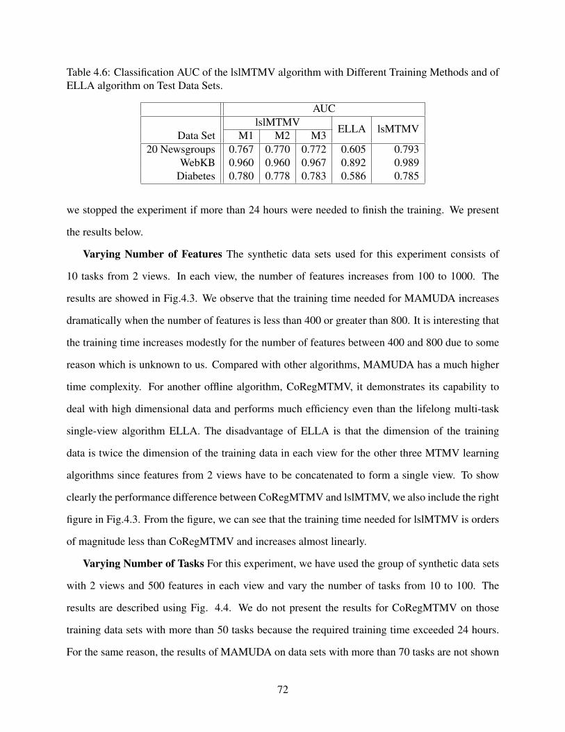
Table 4.6: Classification AUC of the lslMTMV algorithm with Different Training Methods and ofELLA algorithm on Test Data Sets.

AUClslMTMV

ELLA lsMTMVData Set M1 M2 M3

20 Newsgroups 0.767 0.770 0.772 0.605 0.793WebKB 0.960 0.960 0.967 0.892 0.989

Diabetes 0.780 0.778 0.783 0.586 0.785

we stopped the experiment if more than 24 hours were needed to finish the training. We present

the results below.

Varying Number of Features The synthetic data sets used for this experiment consists of

10 tasks from 2 views. In each view, the number of features increases from 100 to 1000. The

results are showed in Fig.4.3. We observe that the training time needed for MAMUDA increases

dramatically when the number of features is less than 400 or greater than 800. It is interesting that

the training time increases modestly for the number of features between 400 and 800 due to some

reason which is unknown to us. Compared with other algorithms, MAMUDA has a much higher

time complexity. For another offline algorithm, CoRegMTMV, it demonstrates its capability to

deal with high dimensional data and performs much efficiency even than the lifelong multi-task

single-view algorithm ELLA. The disadvantage of ELLA is that the dimension of the training

data is twice the dimension of the training data in each view for the other three MTMV learning

algorithms since features from 2 views have to be concatenated to form a single view. To show

clearly the performance difference between CoRegMTMV and lslMTMV, we also include the right

figure in Fig.4.3. From the figure, we can see that the training time needed for lslMTMV is orders

of magnitude less than CoRegMTMV and increases almost linearly.

Varying Number of Tasks For this experiment, we have used the group of synthetic data sets

with 2 views and 500 features in each view and vary the number of tasks from 10 to 100. The

results are described using Fig. 4.4. We do not present the results for CoRegMTMV on those

training data sets with more than 50 tasks because the required training time exceeded 24 hours.

For the same reason, the results of MAMUDA on data sets with more than 70 tasks are not shown

72

0 200 400 600 800 10000

1000

2000

3000

4000

5000

6000

7000

8000

9000

# of featuresseconds

MAMUDA

ELLA

CoRegMTMV

lslMTMV

0 200 400 600 800 10000

50

100

150

200

250

# of features

seconds

CoReg

lslMTMV

Figure 4.3: Training time comparison of different algorithms on synthetic data set with varyingnumber of features from 100 to 1000. Left: Comparison of lslMTMV with other three baselinealgorithms. Right: Comparison of lslMTMV with CoRegMTMV

0 20 40 60 80 1000

2

4

6

8

10x 10

4

# of tasks

seconds

CoReg

MAMUDA

ELLA

lslMTMV

0 20 40 60 80 1000

1000

2000

3000

4000

5000

# of tasks

seconds

ELLA

lslMTMV

0 20 40 60 80 1000

5

10

15

20

25

# of tasks

seconds

lslMTMV

Figure 4.4: Training time comparison of different algorithms on synthetic data set with varyingnumber of tasks from 10 to 100. Left: Comparison of lslMTMV with other three baseline algo-rithms. Middle: Comparison of lslMTMV with ELLA. Right: Performance of lslMTMV

here. We observe that the training time for CoRegMTMV increases exponentially although it

achieves much better performance than MAMUDA and ELLA when the number of tasks is less

than 40. Thus there is difficulty for it to be applied to the training data with large number of tasks.

The training time for MAMUDA increases almost linearly when the number of tasks is less than

70 and has a dramatic growth when there are more tasks. Compared with the two lifelong learning

algorithms, ELLA and lslMTMV, the training time for MAMUDA is over ten times longer than

ELLA and thousands of times longer than lslMTMV. This demonstrates the efficiency of lifelong

learning algorithms when more and more tasks coming in. From the comparison between two

lifelong learning algorithms, we see that lslMTMV achieves two orders of magnitude speedup in

training time.

Varying Number of Views The group of synthetic data sets generated for this experiment

contain 10 tasks and 500 features in each view while the number of views vary from 2 to 20.

73

0 5 10 15 200

0.5

1

1.5

2

2.5x 10

4

# of viewsseconds

CoReg

MAMUDA

lslMTMV

0 5 10 15 200

10

20

30

40

50

60

70

80

# of views

seconds

lslMTMV

Figure 4.5: Training time comparison of different algorithms on synthetic data set with varyingnumber of views from 2 to 20. Left: Comparison of lslMTMV with CoRegMTMV and MA-MUDA. Right: Performance of lslMTMV

We describe the results using Fig. 4.5. We did not carry out this experiment for ELLA since

it can only handle sing-view data. For MAMUDA, the training time is much higher than the

other two algorithms when the number of views is less than 8. However, it achieves almost the

same efficiency as CoRegMTMV when the number of views is 8 and outperforms it after that.

MAMUDA has an almost linear growth although the increase is rather steep. For CoRegMTMV,

we only show the results for data set with less than 10 views due to the training time needed

for each data set with more views exceeded 24 hours. Compared with other two algorithms, the

growth of training time for CoRegMTMV increases exponentially and can hardly be scaled to data

set with large number of views. lslMTMV has achieved much better scalability than the other

offline algorithms with more than two orders of magnitude less time.

4.5 Conclusion

In this work, we first propose a latent space based MTMV learning algorithm, lsMTMV, to improve

prediction models by utilizing task relatedness and consistency among multiple views. Then we

adapt it to a lifelong setting and propose an algorithm for lifelong MTMV learning, lslMTMV.

lslMTMV can effectively handle new tasks and new views which may arrive at any time during

learning process. Furthermore, it achieves lower computational cost through various techniques.

74

Chapter 5

Constructivism Learning

5.1 introduction

Developing transparent predictive analytics has attracted significant research attention recently

[Amershi et al., 2014, Burrell, 2016]. There are many applications where transparent models are

critical for the successful deployment of such systems. For example in the medical domain, it

is hard for a physician to use results from predictive modeling without knowing how the results

are derived. To better train robots, Thomaz and Breazeal showed that if a learning algorithm

can reveal its uncertainty of an action in reinforcement learning, that information provides great

help for human to better train robots [Thomaz & Breazeal, 2006]. In addition in legal system for

recidivism prediction, using black box predictive analytics may lead to unfair treatment of minority

groups and thus commit illegal discrimination [Zeng et al., 2016].

There is intensive discussion on how to define transparency and how to introduce transparency

in a predictive analytics. There is a large body of literature focuses on explaining the results of

the prediction [Hara & Hayashi, 2016, Kim, 2015]. The premise is that if we are able to explain

the model results, we improve the transparency of the model and in this sense interpretability and

transparency are two closely interleaved concepts. Exemplar work in this category includes sparse

linear models [Ustun & Rudin, 2016], prototype based methods such as Bayesian case models

[Kim et al., 2014], and approximating opaque models using local and interpretable models such as

decision trees [Ribeiro et al., 2016], among others. Additional theoretic model includes Situated

Learning Theory [Thomaz & Breazeal, 2006], regarding human learning in the context of social

interactions and “black box in a glass box” [Höök, 2000, Laura Chiticariu & Reiss, 2015] where

75

different levels of modeling transparency are discussed.

The critical limitation of existing discussion is that all the aforementioned works focus on either

making sense of the produced model to or delivering models that are easily understandable by end

users. They do not aim to understand the internal and often complicated modeling process. We

view machine learning decision process as a process of “trade-off” between model fitness (usually

evaluated by a loss function) and modeler’s experience (usually encoded as the prior distribution

in Bayesian learning or the regularization in PAC learning). We argue that in order to achieve

transparency we have to at least reveal the internal trade-off process that involves features, hyper-

parameters, learning machines, and key results statistics, to the end user as advocated for example

in [Zhou et al., 2013].

Our work is motivated by a much broader philosophical discussion called “constructivism",

which has profound impact of modern viewpoint about the nature of knowledge. In the construc-

tivism theory, the learner constructs new knowledge through her interaction with the world with

two key processes assimilation and accommodation. Through assimilation, a learner incorporates

new experience into an existing knowledge framework without changing that framework. Through

accommodation, a learner changes her internal representation of the external world according to

the new experience.

With this intuition, we propose a new learning paradigm where when we have new interactions

with the world (i.e. through a new training sample), we evaluate whether existing knowledge can

generalize well to this new interaction with minor modifications. If not we conclude that new

knowledge should be constructed. Specifically in the context of data analytics, we assume samples

arrive sequentially. For each newly introduced sample we evaluate our trained models and decide

whether we should simply update the existing models (assimilation) or we should create a new

learning model since we have sufficient evidence to believe that there is a new learning task in our

data sets (accommodation). Here “we” is a machine learning algorithm.

We formalized a Bayesian nonparametric approach using sequential Dirichlet Process Mixture

Models (DPMM) to support constructivism learning. The advantage of Bayesian nonparametric

76

is that we do not need to specify the total number of classification models up front and we use

data driven approaches to explore a set with potentially infinite number of models. At the core of

this new DPMM we aim to evaluate whether a newly introduced sample belongs to a particular

classification task. For that we introduced a technique called the selection principle to improve the

fitness principle, which is commonly used in traditional Dirichlet Process Mixture of models.

In summary the major contributions that we made in this paper towards transparent predictive

analytics are highlighted below.

• We introduced the theory of constructivism in order to offer transparency in the learning

process using two concepts: assimilation and accommodation. Based on the theory, we

designed a principled approach called constructivism learning.

• We launched a systematic investigation and formalized the related learning problem as a

novel sequential Dirichlet Process Mixture of Classification Model problem (a.k.a. sDPMCM)

where with new training samples we may either update existing learning models or identify

a new learning task.

• We introduced a novel and efficient variational inference method for sDPMCM with a tech-

nique that we call selection principle.

• Our experimental study confirmed the efficiency of the new learning paradigm and showed

that the new paradigm revealed useful insights and improved transparency of the modeling

process.

5.2 Related Work

We review related work in three highly relevant categories: transparent machine learning, con-

structivism (human) learning, and task construction in functional data analysis.

77

5.2.1 Transparent Machine Learning

We notice that there are a few recent efforts aiming to reveal the underlying reasoning mechanics

of a machine learning algorithm. For example Krause et al. [Krause et al., 2016] employed a vi-

sual analytics to depict input-output relationship by treating the algorithm as a black-box. In this

way the user gets a sense of internal learning process by observing how the output may change

according to the change of input. Zhou et al. [Zhou et al., 2013] developed a technique to improve

transparency by revealing the internal status of a hierarchical beta process. In their study they vi-

sualize how output statistics (e.g. precision, recall) change according to different hyperparameter

settings. However we lack principled and systematic approaches to address the problem. To ini-

tialize the discussion in this paper we adopted the theory of constructivism in human learning and

designed an approach with comprehensive experimental study.

5.2.2 Constructivism Learning

We briefly review the constructivism theory in order to provide further background information

and motivation of our work. The full treatment of the concept is clearly beyond this technical

discussion and useful references can be found in [Piaget, 1985]. Constructivism aims to better

understand the nature of knowledge and thus it belongs to epistemology, a branch of philosophy

dated back to Aristotle. In that constructivism is not merely a pedagogy though it has been widely

used in designing education methods. Following constructivism in education, the focus is to change

the role of an educator from a supervisor to a facilitator. Construtivism thus promotes active

learning where instructor provide all the necessary information aiming to help students acquire

new knowledge.

5.2.3 Learning with Task Construction

Dynamically identifying learning tasks using Bayesian non-parametrics have been identified in

different context, primarily in functional data clustering [Jacques & Preda, 2014]. In functional

78

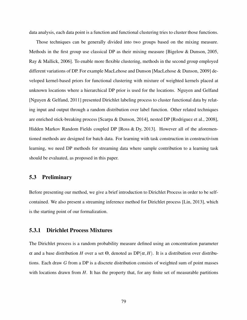
data analysis, each data point is a function and functional clustering tries to cluster those functions.

Those techniques can be generally divided into two groups based on the mixing measure.

Methods in the first group use classical DP as their mixing measure [Bigelow & Dunson, 2005,

Ray & Mallick, 2006]. To enable more flexible clustering, methods in the second group employed

different variations of DP. For example MacLehose and Dunson [MacLehose & Dunson, 2009] de-

veloped kernel-based priors for functional clustering with mixture of weighted kernels placed at

unknown locations where a hierarchical DP prior is used for the locations. Nguyen and Gelfand

[Nguyen & Gelfand, 2011] presented Dirichlet labeling process to cluster functional data by relat-

ing input and output through a random distribution over label function. Other related techniques

are enriched stick-breaking process [Scarpa & Dunson, 2014], nested DP [Rodriguez et al., 2008],

Hidden Markov Random Fields coupled DP [Ross & Dy, 2013]. However all of the aforemen-

tioned methods are designed for batch data. For learning with task construction in constructivism

learning, we need DP methods for streaming data where sample contribution to a learning task

should be evaluated, as proposed in this paper.

5.3 Preliminary

Before presenting our method, we give a brief introduction to Dirichlet Process in order to be self-

contained. We also present a streaming inference method for Dirichlet process [Lin, 2013], which

is the starting point of our formalization.

5.3.1 Dirichlet Process Mixtures

The Dirichlet process is a random probability measure defined using an concentration parameter

α and a base distribution H over a set Θ, denoted as DP(α,H). It is a distribution over distribu-

tions. Each draw G from a DP is a discrete distribution consists of weighted sum of point masses

with locations drawn from H. It has the property that, for any finite set of measurable partitions

79

A1,A2, · · · ,Ak of Θ,

(G(A1),G(A2), · · · ,G(Ak))∼ Dir(αH(A1),αH(A2), · · · ,αH(Ak))

Where Dir denotes a Dirichlet distribution.

Consider drawing i.i.d sequence θ1,θ2, · · ·θn ∼ G, the predictive distribution of θi conditioned

on other θ j, j < i, written θ−i is:

θi|θ−i =1

α +n−1 ∑j<i

δθ j +α

α +n−1H (5.1)

Note that (5.1) implies clustering property of DP, i.e., θs in the same cluster have the same value,

due to the positive probability that θi will take on the same value as other θ−i.

Relying on this clustering property of DP, we formalize DP mixture of classification models

for data (xi,yi), i ∈ [1 : N], where xi is a feature vector and yi is a label, as follows:

yi|xi,β i ∼ Fy(·|xi,β i)

xi|θ i ∼ Fx(·|θ i)

(θ i,β i)|G∼ G

G∼ DP(α,Hθ ×Hβ ) (5.2)

Here we model the joint distribution of xi and yi and assume that the base distribution Hθ ×Hβ

is independent between parameters θ i and β i. Through this formulation, data are grouped into

different clusters with each cluster k represented by a generative model parameterized by (θ ∗k ,β∗k).

We have θ i = θ∗k and β i = β

∗k if (xi,yi) is generated using the model of cluster k. Fx and Fy are

generative probabilistic models.

80

5.3.2 Sequential DP Mixture Models (sDPMM)

To handle streaming data for the following generic DP mixture model:

xi|θ i ∼ F(·|θ i)

θ i|G∼ G

G∼ DP(α,H)

Lin proposed a sequential variational approximation method [Lin, 2013]. The advantage of

Lin’s method is that it is truncation free and a single pass over data can reliably estimate a DP

mixture model. In this method suppose θs are grouped into K clusters, and there is a cluster

indicator ci for each θ i,∀i ∈ [1 : N] such that θ i belongs to the kth cluster, i.e., θ i = θ∗k , if ci = k.

Lin proposed to approximate distribution:

p(G|x1:N) = ∑c1:N

p(c1:N |x1:N)p(G|c1:N ,x1:N)

using a tractable distribution with the following form:

q(G|x1:N) = ∑c1:N

(N

∏i=1

ρ(ci))q(c)ν (G|c1:N).

Here θ∗k ∼ νk, which is an independent distribution. The task of inference is to optimize two sets

of parameters ρ , (ρ1,ρ2, · · · ,ρi) and νi , (ν i1),ν

i2, · · · ,ν i

K) so that q(G|x1:N) best approximates

the true posterior p(G|x1:N).

By using variational approximation technique to minimize the Kullback-Leibler divergence

between the true posterior and the approximate posterior, we have sequential approximation for

81

the optimal settings of ρi+1 and ν i+1 after processing i samples:

ρi+1 ∝

wi

k

´θ

F(xi+1|θ)ν ik(dθ) k ≤ K

α´

θF(xi+1|θ)H(dθ) k = K +1

(5.3)

Where wik = ∑

ij=1 ρ j(k).

νi+1k (dθ) ∝

H(dθ)∏

i+1j=1(F(x j|θ))ρ j(k) k ≤ K

H(dθ)(F(xi+1|θ))ρi+1(k) k = K +1(5.4)

ρi(k), ∀k ∈ [1 : K +1], i = 1,2, · · · , are computed using:

ρi(k) =wi−1

k exp(hi(k))

∑K+1c=1 wi−1

c exp(hi(c))(5.5)

Where hi(k) is marginal log-likelihood of xi belonging to cluster k.

5.4 Algorithm

In this section, we describe our proposed algorithm for constructivism learning (CL). We begin by

formalizing the problem setting of CL. This is followed by the description of our sequential DP

mixture of classification model(sDPMCM). Then we propose an improved version of sDPMCM

, sequential DP mixture of classification model with selection (sDPMCM-s), which is enhanced

using an approach we call the selection principle. In the last section, we present the sequential

variational inference algorithm for sDPMCM-s adapted from [Lin, 2013].

5.4.1 Notation

For clarity, we introduce the following notations. We use lowercase letters to represent scalar

values, lowercase letters with bold font to represent vectors (e.g. u), uppercase bold letters to

82

represent matrices (e.g. A), Greek letters α,λ ,γ, . . . to represent parameters. Given a matrix

A = (ai, j) ∈ Rp×k , |A| is the determinant of A. Unless stated otherwise, all vectors in this paper

are column vectors. uT is the transpose of the vector u. We use [1 : N] to denote the set 1,2, . . . ,N.

5.4.2 Problem Setting and Challenges

Suppose that we have data that arrives sequentially, we aim to determine whether newly arrived

sample (xi,yi) can be well classified using existing tasks constructed from previous data (x j,y j),

j = 1,2, . . . , i− 1, or a new task needs to be constructed from scratch. Here xi ∈ Rd is a feature

vector and yi ∈ 0,1 its corresponding label. Giving a sequence of training samples (xt ,yt),

indexed by t, the outcome of our learning algorithm is a set of classification models.

There are two technical challenges. First the number of tasks needed for the training data is not

known a priori. Second the assignment of a sample to a classification task needs to be determined.

Our setting is different from the classical machine learning setting where all the data belong to one

model, or the setting for multi-task learning where we know which task a sample belongs to.

To determine the number of tasks, a common strategy is to use model selection to pick the

“optimal” one from a range of arbitrary numbers. However model selection would incur substantial

computational costs and the search space that contains the optimal number is difficult to determine.

Furthermore, it is suboptimal for streaming data to use a pre-specified number of tasks. To tackle

this, we resort to Bayesian nonparametric models that have infinite-dimensional space. Given a

finite number of samples, only a finite subset of parameter dimensions is needed. This enables that

the complexity of models adapts to data so that the number of tasks can be inferred from the data.

For the second challenge, we rely on the clustering property of DPMM models. In DPMM,

the decision of assigning a sample to a task is based on the fitness principle, i.e., evaluating the

likelihood that the sample is generated from the task. The drawback of this principle is that the

contribution of a sample to a task is ignored. When DPMM is applied to streaming data for

classification models, this may lead to undesirable tasks since they are estimated in a single pass

over the data.

83

−5 0 51

2

3

4

5

6

7

8

T1 -T1 +T2 -T2 +

−5 0 51

2

3

4

5

6

7

8

T1 -

T1 +

T2 -

T3 -

T3 +

T4 +

−5 0 51

2

3

4

5

6

7

8

T1 -

T1 +

T2 -

T2 +

Figure 5.1: Issue of Fitness Principle: Left: Gound Truth; Middle: Tasks Constructed withoutUsing the Fitness Principle; Right: Tasks Constructed using the Selection Principle.

We illustrate the problem of fitness principle using a synthetic data set as shown in Fig. 5.1.

Here we have samples from two hidden tasks T1 and T2 (Left panel). We adopted a DPMM, which

outputted 4 tasks, rather than 2. In addition task T4 has only positive samples and T2 has only

negative samples. Moreover the samples in T1 are highly unbalanced. We believe the reason why

DPMM produces large number of single-class tasks is that the samples in those tasks can be well

classified and hence well well fitted. However, those tasks constructed by DPMM based only

on fitness principle can hardly generalize well to unseen samples. Inspired by this observation,

we develop a new DPMM model enhanced with selection principle utilizing Kullback-Leibler

divergence (KLD). It is a complement to the fitness principle. When making assignment decision,

the contribution of a sample to a task is considered.

To handle streaming data, we first adapt the method proposed in [Lin, 2013] to DP mixture of

classification models. Then we modify a variational approximation technique of logistic regression

[Jaakkola & Jordan, 2000] to achieve efficient parameter updating.

5.4.3 Sequential DP Mixture of Classification Model

In this section, we introduce the details of sequential DP mixture of classification models we use for

CL. We first present the formulation of DP mixture of classification model using logistic regression

as classification models within a task. This poses a challenge for model estimation of streaming

data because the computation of posterior and posterior predictive are intractable. To tackle this,

we introduce the variational approximation technique for logistic regression.

84

5.4.3.1 DP Mixture of Classification Model

The DP Mixture of Classification Model (DPMCM) we use for CL is based on the general formu-

lation (5.2). Here we model the joint distribution of x and y, p(x,y) = p(y|x) p(x), instead of only

modeling the conditional distribution p(y|x). This provide us the benefit of discovering hidden

structure of data by clustering x [Shahbaba & Neal, 2009]. Within each task of the mixture, we as-

sume that x follow a Multivariate Normal (MN) distribution with mean mx and covariance matrix

Σx. For simplicity of computation, we assume a conjugate prior, Normal-Inverse-Wishart(NIW),

for (mx,Σx). To model the relationship between x and y, we use logistic regression:

Fy(y|x,β ) =exp(yxT β )

1+ exp(xT β )(5.6)

Where β ∈ Rd . And we use a Multivariate Normal distribution for βy with parameters (µβ

0 ,Ψβ

0 ).

Note that we assume independence between (mx,Σx) and βy, and the distribution of y does not

depend on (mx,Σx) given x. This results in simplified computations.

The complete DPMCM for CL is summarized as follows:

G∼ DP(α,NIW(µx0,κ

x0 ,Ψ

x0,ν

x0)MN(µ

β

0 ,Ψβ

0 )) (5.7)

For i = 1,2, . . . , draw i.i.d using:

yi|xi,βyi ∼ Fy(·|xi,β

yi )

xi|mxi ,Σ

xi ∼MN(·|mx

i ,Σxi )

(mxi ,Σ

xi ,β

yi )|G∼ G

(5.8)

Due to the clustering property of DP, Θ = (mxi ,Σ

xi ,β

yi ) will be grouped into different clusters.

Θs in the same cluster have an identical value.

85

Different from sDPMM model where only x is clustered, we cluster both x and y by modeling

the joint distribution of x and y. Thus sDPMM cannot be directly applied to DP mixture of classi-

fication models. The main change required here is to modify the sequential approximation of ρi+1

and ν i+1 as follows :

ρi+1 ∝wi

k

´Θ

F(xi+1,yi+1|Θ)ν ik(dΘ) k ≤ K

α´

ΘF(xi+1,yi+1|Θ)H(dΘ) k = K +1

(5.9)

νi+1k (dΘ) ∝H(dΘ)∏

i+1j=1(F(x j|µx,Σx)F(y j|β y))ρ j(k) k ≤ K

H(dΘ)(F(xi+1|µx,Σx)F(yi+1|β y))ρi+1(k) k = K +1(5.10)

5.4.3.2 Variational Approximation of Logistic Regression

Using logistic regression to model the relationship between x and y poses challenges for computing

posterior distribution of model parameters and predictive distribution since they are computation-

ally intractable. To tackle this, we adopt the variational approximation proposed in [Jaakkola & Jordan, 2000]

to replace the logistic function with an adjustable lower bound that has a Gaussian form. This re-

sults in the Gaussian form of posterior due to the Gaussian prior of βy and Gaussian variational

form of p(y|x,β y,ξ ). Here ξ is a variational parameter. Then the approximate Bayesian updates

take the following form when receiving a new sample (xi+1,yi+1):

Ψβ

i+1 =[(Ψ

β

i )−1 +2 f (ξ )xi+1xT

i+1

]−1

µβ

i+1 = Ψβ

i+1

[(Ψ

β

i )−1

µβ

i +(yi+1−12)xi+1

]

86

Where f (ξ ) = tanh(ξ/2)/(4ξ ). And the closed-form update equation for ξ is

ξ2 = xT

i+1Ψβ

i+1xi+1 +(xTi+1µ i+1)

2

To use this variational approximation for DPMM in sequential setting, we need to modify the

updating of parameters Ψβ ,µβ ,ξ so that the uncertainty of clustering brought by sequential infer-

ence can be incorporated. With straightforward calculation, we derive the following modification

to the updating of parameters when ρi+1 > 0:

Ψβ

i+1 =[(Ψ

β

i )−1 +2ρi+1 f (ξ )xi+1xT

i+1

]−1

µβ

i+1 = Ψβ

i+1

[(Ψ

β

i )−1

µβ

i +(ρi+1yi+1−12)xi+1

](5.11)

ξ2 = ρi+1

[xT

i+1Ψβ

i+1xi+1 +(xTi+1µ

β

i+1)2]

For the predictive lower bound for sample xi+1,yi+1, it takes the form:

lnq(yi+1|xi+1,D) = lng(ξi+1)−ξi+1

2+ f (ξi+1)ξ

2i+1

− 12(µ

β

i )T (Ψ

β

i )−1

µβ

i

+12(µ

β

i+1)T (Ψ

β

i+1)−1

µβ

i+1

+12

ln|Ψβ

i+1|

|Ψβ

i |(5.12)

Where D = (x1,y1),(x2,y2), . . . ,(xi,yi).

87

s1 s2 s3 s4KLD 4.485 4.486 4.547 4.491

Pr 0.972 0.967 0.729 0.953

Table 5.1: Comparison of KLD and Posterior Predictive Probability (Pr)

5.4.4 Sequential DP Mixture of Classification Model with Selection Princi-

ple (sDPMCM-s)

5.4.4.1 Selection Principle

In selection principle, we focus on evaluating the contribution of a sample to a task. Specially, we

aim to measure the utility of an observation of a random variable, i.e. a sample, to other random

variables, i.e., task parameters. To this end, we utilize Kullback-Leibler divergence (KLD). This

technique has been used in Bayesian optimal experiment design (BOED) [Ryan et al., 2015] to

select the optimal design of experiment so that the expected utility of the experiment outcome can

be maximized. Different from the general case in BOED, we focus on the utility of a given sample

instead of the expected utility. Specifically, we assign a sample to a task so that KLD between the

prior distribution of task parameters and the posterior given the sample is maximized. Suppose we

have a sample (x,y) and task parameters βy, the utility is defined as:

U(β y;x,y) = DKL(p(β y|x,y) ‖ p(β y))

The goal of selection principle is to assign a sample (x,y) to a task with parameter βy such that

U(β y;x,y) is maximized. To understand the function of selection principle, we illustrate it using

Fig. 5.2 and Table 5.1. In this example we selected four representative samples in a task. s1 and

s2 are mean of positive and negative samples separately. s3 is close to decision boundary. s4 is far

away from decision boundary. We observe that although s1, s2, s4 have higher posterior predictive

probabilities, their utility to the task is lower than s3. This example confirms our hypothesis that

the selection principle can act as a regularization factor to regulate the range of a task to form more

compact clusters.

88

−22 −20 −18 −16 −14 −12 −10 −81

2

3

4

5

6

7

8

9

S1

S2

S3

S4

Figure 5.2: Function of Selection Principle: s1: mean of positive samples; s2: mean of negativesamples; s3: close to decision boundary; s4; far away from decision boundary.

5.4.4.2 Applying Selection principle

To incorporate selection principle when making assignment decision, we modify the computation

of task assignment probability ρi+1 as follows:

ρi+1 ∝

wi

ksi+1k

´Θ

F(xi+1,yi+1|Θ)ν ik(dΘ) k ≤ K

αsi+1k

´Θ

F(xi+1,yi+1|Θ)H(dΘ) k = K +1(5.13)

Where si+1k = exp(γU(β y;xi+1,yi+1)), where γ is a coefficient to regularize the effect of selection

principle. Through si+1k , the utility of xi+1,yi+1 to the model parameter β

y is also considered when

making task assignment decisions.

5.4.5 Inference

Several issues need to be addressed for the inference of the proposed sDPMCM-s for streaming

data. First, an efficient method is needed to compute U(β y;(x,y)) when new samples arrive. Sec-

ondly, posterior distribution for Θ and prediction distribution for x and y needs to be updated with

relatively low complexity during streaming inference. Thirdly, the inference method, i.e. sDPMM,

proposed by Lin was designed for DPMM instead of DPMCM. Thus some modification is needed

to adapt it to DPMCM. The first two problems can be directly solved with the adoption of vari-

89

ational approximation for logistic regression and the using of conjugate prior for µx,Ψx. For the

third problem, we adopt the modification of approximation of proposed in (5.9) and (5.10) to clus-

ter both x and y.

In the following, we give the specific formula for utility computation, describe the details of

sequential inference for sDPMCM-s and introduce the strategy we use for prediction.

5.4.5.1 Utility Computation

The computation of U(β y;xi+1,yi+1) is straightforward after the variational approximation is used

for logistic regression. Let denote the distribution as pi(βy | µβ

i ,Ψβ

i ) before (xi+1,yi+1) is assigned

to a model and pi+1(βy | µ

β

i+1,Ψβ

i+1) after assignment, we can calculate the KLD of two MN

distributions pi and pi+1:

U(β y;xi+1,yi+1) =12

[ln|Ψβ

i ||Ψβ

i+1|−d + tr((Ψβ

i )−1

Ψβ

i+1)+

(µβ

i −µβ

i+1)T (Ψ

β

i )−1(µ

β

i −µβ

i+1)]

5.4.5.2 Sequential Inference for sDPMCM-s

To handle streaming data, we consider the method proposed in [Lin, 2013]. The advantage of this

method is that it starts with one model and increases the number of models on the fly when existing

models cannot generalize well to new samples. Specifically, when a new sample arrives, we first

determine whether it will be assigned to an existing task or a new task. Then the model parameters

of assigned task are updated. We describe these two steps separately in the following.

Task Assignment. To determine which task a newly arriving sample belongs to, we need to

compute the assignment probability ρi+1 based on (5.9) and (5.10). The probability of assigning

newly arrived sample (xi+1,yi+1) to task k, denoted as ρi+1(k), is computed using:

ρi+1(k) =wi

ksi+1k exp(hi+1(k))

∑K+1c=1 wi

csi+1c exp(hi+1(c))

(5.14)

90

Where hi+1(k) is the log posterior predictive of (xi+1,yi+1) belonging to cluster k. It can be de-

composed into two parts hi+1(k) = hxi+1(k)+hy

i+1(k). Due to the conjugate property, the posterior

predictive, i.e. hxi+1(k), is a multivariate t distribution with density function:

Γ [(δi +d)/2]Γ(δi/2)δ d/2πd/2|Φi|1/2

[1+

1δi(x−υ i)

TΦ−1i (x−υ i)

](5.15)

Where

δi = νxi (k)−d +1

υ i = µxi (k)

Φi =κx

i (k)+1κx

i (k)(νxi (k)−d +1)

Ψxi (k)

µxi (k),Ψ

xi (k),κ

xi (k),ν

xi (k) are posterior parameters of a NIW distribution for task k after re-

ceiving i samples. With (5.15), hxi+1(k) can be computed directly.

For the computation of hyi+1(k), we use the lower bound specified in (5.12) derived from a

variational approximation of logistic regression.

Updating Model parameters. Relying on the conjugate property, posterior parameters of the

NIW distribution of task k have a closed-form updating when receiving a new sample xi+1. For

simplicity, we update natural parameters Λ = (η1i (k),η

2i (k),η

3i (k),η

4i (k)) of NIW distribution for

task k at each step. They can be derived from µxi (k), Ψx

i (k), κxi (k), νx

i (k) using:

η1i (k) = κ

xi (k)µ

xi (k)

η2i (k) = κ

xi (k)

η3i (k) = Ψ

xi (k)+κ

xi (k)µ

xi (k)(µ

xi (k))

T

η4i (k) = ν

xi (k)+d +2

Modified from the sufficient statistics of the NIW distribution [Foti et al., 2014], the following

91

form of updating for Λ with considering the uncertainty of task assignment are used:

η1i+1(k) = η

1i (k)+ρi+1(k)xi+1

η2i+1(k) = η

2i (k)+ρi+1(k)

η3i+1(k) = η

3i (k)+ρi+1(k)xi+1(xi+1)

T

η4i+1(k) = η

4i (k)+ρi+1(k)

For the updating of parameters µβ

i ,Ψβ

i for βyi , we use the variational approximation in (5.11).

5.4.5.3 Prediction

For predicting the label of a test sample x, we use the following strategy. First, we use all the

K tasks learned from training data to predict the label of x to get K labels, y1, y2, . . . , yK . Then

we compare the posterior predictive of P(x, yk), ∀k ∈ [1 : K] and set the label of x to yk∗ so that

P(x, yk∗) = max(P(x, y1),P(x, y2), . . . ,P(x, yK)).


In this section, we first introduce the data sets and experimental protocol used in our experi-

ments. Then we evaluate the performance of our proposed methods, sDPMCM and its variation

sDPMCM-s, by comparing them with base-line methods SVM, Random Forest, and a state-of-

the-art classification model based on enriched Dirichlet Process Mixture model (EDPMM) on 4

synthetic data sets and 3 real-world data sets. Lastly, we demonstrate how transparency can be

improved through task construction.

5.5.1 Data Sets

For the experiments, we used both synthetic data sets and real-worlds data sets, as detailed below.

92

5.5.1.1 Synthetic Data Sets

we constructed 4 synthetic data sets with K hidden tasks each, where K ∈ [2 : 5]. For each task,

we randomly draw its parameters from a NIW prior and a MN prior. For the NIW prior of mx

and Σx, we use zero mean and a diagonal scale matrix ψ0I, where ψ0 = 2. We set κx0 = 0.04 and

degree of freedom νx0 = d + 3, where d is the dimension of x. For the MN prior of β

y, we use a

MN distribution with zero mean and a unit diagonal covariance matrix. The data x,y are generated

using the distribution described in (5.16). We summarize the statistics of 4 synthetic data sets in

Table 5.2.

yi|xi,βyi ∼ Fy(·|xi,β

yi )

xi|mxi ,Σ

xi ∼MN(·|mx

i ,Σxi )

(5.16)

Data Set SDS1 SDS2 SDS3 SDS4T 2 3 4 5N 205 317 406 500

Table 5.2: Statistics of Synthetic Data Sets. T: Number of Hidden Tasks. N: Number of Samples.

5.5.1.2 Real-world Data Sets

We used 3 real-world data sets: WebKB, School Performance and Landmine.

WebKB. This data set contains a subset of the web pages collected from computer science de-

partments of 4 universities in January 1997 by the World Wide Knowledge Base (WebKb) project

of the CMU text learning group 1. It is composed of 230 course pages and 821 non-course pages.

For each web page, two types of representation are provided, text on the web page and anchor text

of the hyperlinks to that page. We generate the features from text on the web pages using TF-IDF.

1http://www.cs.cmu.edu/afs/cs/project/theo-20/www/data/

93

http://www.cs.cmu.edu/afs/cs/project/theo-20/www/data/

Then we applied PCA to the features to keep the first 30 components. The classification goal here

is to determine whether a web page is a course page or not.

School Performance. The school data set comes from the Inner London Education Authority

(ILEA). It is composed of examination records from 140 secondary schools in years 1985,1986

and 1987. The original data includes the year of examination, 4 school-specific attributes and

3 student-specific attributes. In our experiments, we use the processed data set provided by

[Argyriou et al., 2008], where categorical features are expressed as binary features. To use this

data set for classification, we labeled those samples with examination scores larger than 30 as pos-

itive and others as negative. We use data from 123 schools by removing those schools with less

than 5 positive or 5 negative samples.

LandMine. The land mine data set [Ruvolo & Eaton, 2013b, Xue et al., 2007] consists of

14,820 samples from 29 different geographical regions. The features are extracted from radar

data, including four-moment based features, three correlation-based features, one energy-ratio fea-

ture, one spatial variance feature, and a bias term. The classification goal is to detect whether or

not a land mine is present in an area. We used 20% of the data for our experiments.

For each data set, we randomly chose 50% of the data for training and the other 50% for testing.

We applied bootstrap resampling to training data sets to create balanced data sets. The statistics

about 3 data sets are summarized in Table 5.3.

Data Set N dWebKB 1051 30School 11966 17

LandMine 2972 9

Table 5.3: Statistics of Real Data Sets. N: number of samples d: number of features

5.5.2 Experiment Protocol

Baseline Methods. To the best of our knowledge, there is no previous work on learning with

task construction for classification of streaming data. Thus we only compare our methods with

94

two widely applied batch learning methods, SVM and Random Forest, and one state-of-the-art DP

mixture of classification model, joint enriched Dirichlet process mixture model (EDPMM) pro-

posed in [Wade et al., 2014]. For SVM, we used a SVM classifier with a RBF kernel provided

in Matlab. For Random Forest, we used the algorithm implemented in scikit-learn python pack-

age. For EDPMM, we used the R code developed by the original authors. We implemented both

sDPMCM and sDPMCM-s in Matlab.

Model Selection. We performed grid search to select optimal model parameters using 10-fold

cross validation that was performed on the training data.

Evaluation Metrics. We used AUC, the area under a ROC curve, calculated on testing data

only, to compare the performance of different algorithms.

5.5.3 Performance Evaluation Results

To evaluate the performance of our proposed methods, we compared them with 4 baseline methods

on 4 synthetic data sets and 3 real-world data sets.

5.5.3.1 Comparison on Synthetic Data Sets

Table 5.4 presents the results of comparison on 4 synthetic data sets. Compared with SVM and

RF, DP-based methods achieves competitive or better results on 4 data sets. As we expected,

batch DP mixture model, EDPMM, outperforms sDPMCM and sDPMCM-s on the 3 synthetic

data sets. However, the performance difference on SDS1 and SDS2 is not statistically significant

according to the paired student t test. Comparing sDPMCM and sDPMCM-s, we observe that

sDPMCM- always outperforms sDPMCM. This demonstrates the effectiveness of selection prin-

ciple on improving performance. It is worth noting that sDPMCM is comparable with EDPMM

on SDS4 data set. And sDPMCM-s even performs significantly better than EDPMM on this data

set. Our explanation is that the covariance structure may be more complicated with more hidden

tasks. Compared with the Inverse-Gamma distribution adopted by EDPMM, the Inverse-Wishart

distribution we used for sDPMCM and sDPMCM-s allows richer covariance structure.

95

DataSet SVM RF EDPMM sDPMCM sDPMCM-sSDS1 0.812 0.801 0.860 0.847 0.856SDS2 0.787 0.748 0.806∗ 0.788 0.798SDS3 0.814 0.789 0.823 0.813 0.822SDS4 0.823 0.814 0.839 0.838 0.852∗

Table 5.4: Comparison of Algorithms on Synthetic Data Sets. AUC is used for the performancemetric.*: statistically significant with 5% significance level.

5.5.3.2 Comparison on Real Data Sets

DataSet SVM RF EDPMM sDPMCM sDPMCM-sWebKB 0.873 0.896 0.894 0.897 0.910∗School 0.718 0.718 0.676 0.715 0.717

LandMine 0.676 0.670 0.552 0.670 0.687∗

Table 5.5: Comparison of Algorithms on Real Data Sets. AUC is used for the performance met-ric.*: statistically significant with 5% significance level.

We show the results of comparison of algorithms on real data sets in Table 5.5. Compared

with base-line methods, EDPMM achieves similar performance on WebKB data set. However,

its performance on LandMine data set is much worse than those of SVM and RF. There are two

possible reasons. First, as we mentioned before, it is possible that the Inverse-Gamma prior adopted

by EDPMM cannot explain the complicated covariance structure of data. Secondly, EDPMM used

a nested structure to form hierarchical clusters, where X-clusters are nested into each y-cluster.

This choice of ordering X and y may be inappropriate for this data set. Although it is possible

to use a different ordering, this choice is problem specific and the work did not provide a way

to guide this decision. For the school data set, EDPMM also has the worst performance among

all algorithms. But note that we collect the result of EDPMM from one run of the experiment

due to the high computation cost. For our proposed method, sDPMCM, it achieves comparable

performance with random forest. Relying on selection principle, sDPMCM-s achieves statistically

significant advantages over other algorithms on WebKB and Landmine data sets.

96

5.5.4 Transparency Evaluation

To study how the transparency of each model changes when the heterogeneity of data increases,

we primarily focus on synthetic data sets where we know the number of tasks embedded in the

data sets and hence a direct comparison is possible. For real-world data sets, we do not have such

information. We evaluate an indirect metric in order to gain insights of the model transparency.

5.5.4.1 Evaluation on Synthetic Data Sets

We first picked up the data set SDS3 and recorded model complexity of different algorithms with

a increasing number of samples. To evaluate model complexity, for SVM, we record the number

of support vectors. For Random Forest, we record the number of trees and for sDPMCM-s the

number of constructed tasks. The results are shown in Fig. 5.3. In this test, the number of samples

are sequentially introduced in such way that the first n samples are all from one task, then we have

two tasks, three tasks and so on so forth. In Fig. 5.3 we observe the model complexity increases as

we have more samples (or more hidden tasks). sDPMCM-s captures precisely the right number of

hidden tasks.

To further investigate the issue, in Fig. 5.4 we display the tasks constructed when evaluating

sDPMCM and sDPMCM-s on SDS3. With more samples, both algorithms can construct more

tasks to accommodate the data. However, sDPMCM cannot correctly identify those hidden tasks

due to the limitation of only using fitness principle. Although the complexity of models learned

by sDPMCM-s increased in terms of number of tasks, it provides insights into the structure of data

with newly constructed tasks. Compared with SVM and Random Forest, it affords explanation

why higher complexity is needed. We observe the same trend in other synthetic data sets. With the

space limitation, we do not show (similar) figures for other synthetic data sets.

5.5.4.2 Evaluation on Real-World Data Sets

For real-world data sets, we do not know precisely the number of hidden tasks. In addition the

data are in a much higher dimensional space and it is difficult to visualize the cluster structure that

97

54 102 158 202 2490

100

200

# o

f S

V

54 102 158 202 2490

50

100

# o

f T

rees

54 102 158 202 2490

5

10

# o

f T

asks

# of Samples

Figure 5.3: Transparency Evaluation on Synthetic Data Set SDS2. Top: SVM, Middle: RandomForest, Bottom: sDPMCM-s.

−4 −2 0 2 4−2

0

2

4

6

8

10

T1 -T1 +T2 -T2 +T3 -T3 +

−4 −2 0 2 4−2

0

2

4

6

8

10

T1 -

T1 +

T2 +

T3 -

T3 +

T4 -

T5 -

−4 −2 0 2 4−2

0

2

4

6

8

10

T1 -

T1 +

T2 -

T3 -

T3 +

T4 +

Figure 5.4: Tasks Construction Comparison: Left: Ground Truth, Middle: Tasks Constructed bysDPMCM, Right: Tasks Constructed by sDPMCM-s

675 1192 1928 2581 3315 3911 44410

5000

10000

# o

f S

V

675 1192 1928 2581 3315 3911 44410

50

100

# o

f T

rees

675 1192 1928 2581 3315 3911 44410

10

20

# o

f T

asks

# of Samples

Figure 5.5: Transparency Evaluation on School Data Set. Top: SVM, Middle: Random Forest,Bottom: sDPMCM-s.

98

we learned. Therefore we collect statistics regarding model complexity as we did for the synthetic

data. In Fig. 5.5, we show how model complexity changes with increasing number of samples.

Results are averaged over 10 runs at each collected point.

We notice that the number of support vectors of the SVM model consistently increases with

increasing number of samples and the standard deviation across different runs is low. Compared

with SVM, Random Forest and sDPMCM-s are more robust in the sense that the model complexity

are not sensitive to the increasing number of samples. Comparing Random Forest and sDPMCM-

s, we notice that sDPMCM-s are more “stable” in the sense the variance of the number of tasks

across different runs is much smaller. This phenomenon increases our confidence that sDPMCM-s

captures the hiddern but important tasks embedded in the data sets.

5.6 Conclusion

In this work we proposed a new learning paradigm for transparent predictive analytics where we

incorporate a contemporary philosophical concept of constructivism in machine learning. We de-

veloped a model formalization using Dirichlet Process Mixture Models for streaming data with

efficient inference. Our experimental study demonstrated the utility of the proposed methods. Our

future work is to extend the current algorithm to other learning scenarios such as semi-supervised

learning.

99

Chapter 6

Constructivism Learning for Local Dropout Architecture

Construction

6.1 Introduction

Dropout is attracting intensive research interest in deep learning as an efficient approach to prevent

overfitting [Hinton et al., 2012]. In the training phase, for each mini-batch, dropout works by ran-

domly omitting some units from the original deep neural network to create a sub-network. In the

testing phase, dropout simply computes the average of all the explored subnetworks. Since there

is an exponential number of possible sub-networks for a given neural network, it is impractical

to explore all of them and then perform model averaging. This requires huge amount of data and

computing power, even for deep learning. Drop-out circumvents the problem by adding a regular-

ization that all subnetworks must share the same weights on any shared nodes. With the constraint,

the total number of weights need to be trained is still quadratic (assuming a fully connected net-

work) to the number of nodes in the network. The power of dropout for overfitting prevention is

attributed primarily to two factors: model averaging with bagging and model regularization. Both

reduce model variance.

To design better dropout schemes, a large number of studies in the literature have focused on

randomly dropped out some units in a network according to a predefined dropout rate [Gal & Ghahramani, 2016,

Wang & Manning, 2013] or learned distributions on dropout rates [Ba & Frey, 2013, Kingma et al., 2015,

Li et al., 2016, Maeda, 2014, Molchanov et al., 2017]. Recently incorporating “structural” infor-

mation when deciding which units to drop out produced promising results comparing to methods

100

that ignore the structural information. For example the work in [Li et al., 2017, Tompson et al., 2015,

Neverova et al., 2016] proposed to drop out a group of units simultaneously based on prior knowl-

edge such as a specific feature map in a convolutional network or modality related information.

Murdock et al. [Murdock et al., 2016] developed a method, Blockout, to group the units of a net-

work into clusters which are learned from the data and each dropout architecture consists of the

units in a cluster. Both methods have obtained better empirical performance in various applica-

tions.

A major issue of the above mentioned work is that existing work constructed and applied drop

out architectures globally to all the instances. It failed to differentiate among instances when

constructing the dropout architecture. This can be a significant deficiency for certain applications.

For example, when predicting the ratings given by consumers to different restaurants, consumers

may weight the features of a restaurant differently in different activities, such as banquets or dates.

Thus a neural network is more likely to achieve better performance if it has the capability to

differentiate among instances and construct different dropout architectures for them so that varying

weights can be given to the features.

To tackle this issue, we propose a method, CODA, for local dropout architecture construction,

which is inspired from a philosophical theory regarding human learning, constructivism learning

[Piaget, 1985, Li & Huan, 2017]. This theory has had wide-ranging impact on human learning the-

ories. The essence of this theory is that how human acquire knowledge from experiences through

two fundamental processes: assimilation and accommodation. In assimilation, an experience can

be incorporated into a learner’s existing knowledge framework without changing that framework.

In accommodation, new knowledge must be constructed in order to accommodate the experience.

Applying this theory to deep learning, for each instance, the algorithm decides whether an ex-

isting dropout architecture should be used, i.e., assimilation, or a new dropout architecture should

be constructed, i.e., accommodation. We illustrate the concept of constructivism deep learning in

Figure 6.1, where we have a deep neural network (DNN) with two hidden layers, depicted in the

left figure. Given 4 instances (x1,y1),(x2,y2),(x3,y3),(x4,y4), a dropout architecture, depicted

101

(x1, y1), (x2, y2), (x3, y3), (x4, y4) (x1, y1), (x4, y4) (x2, y2), (x3, y3)

Figure 6.1: Constructivism Deep Learning. Left: The Network Architecture of a DNN. Middle andRight: Two Different Dropout Architectures. The first dropout architecture is shared by instances(x1,y1) and (x4,y4). The second dropout architecture is shared by instances (x2,y2) and (x3,y3).

in the middle figure, is constructed and used for the first instance (x1,y1). For the second instance,

since it is quite different from the first instance, accommodation happens and a new dropout archi-

tecture, depicted in the right figure, is constructed for it. For the instance (x3,y3), it triggers the

assimilation process, sharing the same dropout architecture with (x2,y2). It is the similar situation

for (x4,y4), which shares the same dropout architecture with (x1,y1).

There are many challenges in adapting human constructivism learning to deep learning. First,

we need to decide which instances should share the same dropout architecture; Secondly, we need

to decide the optimal dropout architecture for those instances. We opted for Bayesian noparametric

techniques for overcoming those challenges by adopting Uniform Process.

Specially, given an instance, we will determine which dropout architecture should be used

according to the loss of that architecture and the similarity among different instances. Meanwhile,

this process allows new architecture to be selected due to its nonparametric characteristics.

We have laughed a comprehensive experimental study with both synthetic and real-world data

sets. Comparing the performance with other state-of-the-art dropout techniques, the experimental

results demonstrated the effectiveness of our proposed method.

The contributions of this paper is as follows:

• We have adapted human constructivism learning to deep learning for local dropout architec-

ture construction.

• We have designed an algorithm, Uniform Process Mixture Models (UPMM), for construc-

102

tivism deep learning based on a Bayesian nonparametric technique, Uniform Process. In ad-

dition, we have developed an effective inference method for efficient computation of UPMM.

• We have compared our methods with 2 state-of-the-art techniques using 5 real-world data

sets and demonstrated the effectiveness of our method.

6.2 Related Work

In this section, we review two lines of research which are mostly related to our work, dropout

training and constructivism learning.

6.2.1 Dropout Training for Deep Neural Networks

Previous work in dropout training for deep neural networks can be categorized into two groups

based on whether the dropout architectures are determined without or with considering prior

knowledge related structure.

For the methods in the first group, the first study was conducted by Hinton et al. in [Hinton et al., 2012],

where hidden units were randomly selected using a fixed dropout rate for all the units. In re-

cent years, different variations of dropout techniques have been developed by approximating the

original dropout technique [Gal & Ghahramani, 2016, Wang & Manning, 2013] or learning adap-

tive dropout rates through imposing on different distributions, such as multinominal distributions

[Li et al., 2016], Bernoulli distributions [Srinivas & Babu, 2016], distributions based on input ac-

tivities [Ba & Frey, 2013], or employing variational Bayesian inference methods [Kingma et al., 2015,

Maeda, 2014, Molchanov et al., 2017].

To incorporate a priori structural information in determining dropout architectures, Tompson

et al. [Tompson et al., 2015] developed the SpatialDropout method for convolutional networks to

drop out all the units in a feature map simultaneously so that adjacent pixels in the feature map

are either all inactive or all active. Neverova et al. [Neverova et al., 2016] employed the modality

information to drop out the input form a channel to achieve robustness in fusion of multiple modal-

103

ity channels for gesture recognition. Different from utilizing these structural information specific

to some applications, Murdock et al. [Murdock et al., 2016] aimed to construct general dropout

architectures by grouping units into different clusters with learned probabilities. [Li et al., 2017]

extended this idea to multi-modal learning by constructing dropout architectures so that subsets of

units correspond to individual modalities.

It is worth noting that all the aforementioned work has failed to address the issue of learn-

ing structured dropout where different instances may share different dropout architectures or sub-

networks.

6.2.2 Constructivism Learning in Machine Learning

Constructivism learning [Piaget, 1985] provides a comprehensive framework of human cognitive

development. It has been exploited for interactive machine learning [Sarkar, 2016] and extensively

studied in robotic learning [Aguilar & Pérez y Pérez, 2017]. A complete survey in this field is

beyond the scope of this paper and the interested reader may refer to [Stojanov, 2009] for a detailed

discussion.

In our previous work [Li & Huan, 2017], to achieve modeling transparency, we adapted con-

structivism learning to machine learning by taking advantage of Bayesian nonparametric tech-

niques, Dirichlet process mixture models.

Note that in this paper, we adapted constructivism learning to deep learning, which has not

been explored in the above mentioned studies.

6.3 Preliminary

In this section, we first introduce the notations used throughout the paper. Then we give a brief

overview of the Bayesian nonparametric technique, Uniform Process, on which our proposed

method is based.

104

6.3.1 Notations

For clarity, we introduce the following notations. We use lowercase letters to represent scalar

values, lowercase letters with bold font to represent vectors (e.g. u), uppercase bold letters to

represent matrices (e.g. A), Greek letters α,λ ,γ, . . . to represent parameters. Unless stated

otherwise, all vectors in this paper are column vectors. uT is the transpose of the vector u. We use

[1 : N] to denote the set 1,2, . . . ,N.

6.3.2 Uniform Process

To conquer the challenges of adapting constructivism learning to deep learning which we men-

tioned before, we rely on Bayesian nonparametric (BNP) clustering techniques. The advantage

of BNP is that it provides a principled mechanicism for determining the partition of instances by

imposing a prior over the partition. Meanwhile, it allows new clusters to be constructed when the

existing clusters cannot fit a new instance well.

To be specific, we used uniform process (UP) [Jensen & Liu, 2008, Wallach et al., 2010] for

constructivism learning. Uniform process is a variation of Dirichlet Process [Ferguson, 1973].

Different variations of DP has been extensively studied and applied to a wide range of applica-

tions in the machine learning literature [Paisley et al., 2015, Teh et al., 2012]. A implicit priori

property of DP is “rich-get-richer”, i.e., new instances are more likely to be assigned to clusters

with more instances. Thus the sizes of clusters induced by DP are often non-uniform, with a few

very large clusters and some small clusters. Compared with DP, uniform process exhibits uniform

distributions over cluster sizes.

The partition of a set of observed instances, x1,x2, . . . , can be sequentially constructed using UP

as follows. Given that N− 1 instances, x1,x2, . . . ,xN−1, are partitioned into K clusters, let denote

the cluster assignment of xn using an indicator variable cn. Then for a new instance xN , it will be

105

Table 6.1: Notations for CODA

N Total number of instancesM Total number of units in a nerual networkL Total number of labelsD dimension of featuresK Total number of architecturesxn feature vector of the instance nyn label for xn encoded as a 1-of-L binary

vectorzn dropout indicator for instance nz∗k dropout indicator for architecture kcn architecture indicator for instance n

Nk indices of instances assigned to architecture kα Concentration parameter for UP

G0 Base Distribution for UP

either assigned to an existing cluster or a new cluster according to the following probability:

p(cN+1 = k|) =

1

K+αk ≤ K

α

K+αk = K +1

(6.1)

where α is a concentration parameter. It regulates the probability of assigning an instance to a new

cluster. The higher it is, the more likely a new cluster will be constructed for a new instance.

6.4 Algorithm

In this section, we first formalize the problem of COnstructivism learning for local Dropout Architecture

construction (CODA) which we aim to solve. Then we describe the details of our proposed method

using UP of mixture models (UPMM) for CODA. Lastly, we outline the inference method designed

for the computation of UPMM.

Before proceeding to the details of algorithm, for convenience, we summarize important nota-

tions for CODA in Table 6.1.

106

6.4.1 Constructivism Learning for Local Dropout Architecture Construc-

tion (CODA)

Suppose we have a set of instances, denoted as a matrix :

X = [x1;x2; . . . ;xN ]

where each row xn ∈ RD is a row vector and corresponds to an instance, and their corresponding

labels, denoted as a vector y = [y1;y2; . . . ;yN ], yn ∈ [1 : L]. When a deep neural network is trained

using X and y, the previous proposed dropout methods did not consider the possible structure in

data or evaluate the relationship among instances when making decisions about which units to

drop out. Accordingly, the units in the network are randomly selected to omit only according to

the drop out rates, which may be fixed or adaptively learned from the data. To overcome this

limitation, we propose to use COnstructivism learning for local Dropout Architecture construction

(CODA). During the training of a deep neural network, the goal of CODA is to determine:

1. Which instances should share the same dropout architecture for prediction and what the

architecture is?

2. When a new dropout architecture should be constructed?

The above goal characterizes the critical challenge of CODA, that is to recognize assimilation,

assigning an instance to an existing dropout architecture and accommodation, constructing a new

dropout architecture for a instance, which corresponds to two fundamental processes of human

constructivism learning. The solution therefore we seek to implement CODA must have the ca-

pability to address this critical challenge. Specifically, it first needs to have a mechanicism for

clustering instances so that the dropout architecture inferred from those instances are optimal for

the prediction performance of the member instances in that cluster. Secondly, it should afford a

principled way for constructing a new dropout architecture when a instance cannot be well fitted

by existing dropout architectures, which implies the complexity of the model, mainly assessed by

107

the number of dropout architectures or the amount of knowledge learned by the model, needs to be

automatically adaptive to the heterogeneity of the data.

Bayesian nonparametric (BNP) methods has long standing in the literature of statistical and ma-

chine learning. One major characteristics of BNP is that it is endowed with infinite-dimensional pa-

rameter space so that the complexity of model parameters is potentially unbounded and the amount

of knowledge captured by the model increases with increasing number of instances. Counting on

this characteristic, we can devise a model based on BNP to handle accommodation, constructing

new knowledge for an unseen pattern in data. For assimilation, we resort to BNP clustering tech-

niques to decide which instances can share the same dropout architecture, i.e., explained by the

existing knowledge. Specially, we adopt uniform process (UP), a variation of Dirichlet process,

and design a UP of mixture models for CODA, for which we present the details in the following

section.

6.4.2 UP Mixture Models for CODA

Mixture model based on BNP has been widely considered to be one of the most important method

for regression and classification problems [Bastani et al., 2016, Hannah et al., 2011, Shahbaba & Neal, 2009,

Wade et al., 2014]. It utilizes local regression or classification models, such as linear regression or

logistic regression, as basic building blocks for instances partitioned into different clusters, where

instances in the same cluster share the same model. The distribution of cluster assignments is

determined by a mixing measure, which can be a Dirichlet process or different variations of DP.

Generally, the mixture model based on BNP for data X and y assuming the following form:

yn|P∼ f (y|G)

f (y|G) =

ˆF(y|Φ)dG(Φ)

108

where F is formulated by the local model used for each cluster and G is determined by the mixing

measure.

Then for each instance (xn,yn),∀n ∈ [1 : N], the generative process using DP as the mixing

measure takes the form:

yn ∼ F(y|xn,Φn)

Φn|G∼ G

G∼ DP(α,G0) (6.2)

where α is a concentration parameter of DP, which regulates how likely a new cluster will be con-

structed. G0 is a base distribution for model parameters Φn. Due to the almost sure discreteness of

G, some Φ’s will have identical values. Then instances and their corresponding model parameters,

Φ’s, form clusters; and instances in the same cluster will share the same Φ.

In Bayesian nonparametric mixture models for classification or regression, for each cluster

of instances, we need to determine the model parameters Φ, such as regression coefficients in

linear regression. For CODA, however, our goal is to select dropout architectures. To this end,

we parametrize each cluster-specific model with a vector consisting of Bernoulli variables z =

[z1;z2; . . . ;zM], where M is the total number of neural units in a DNN. zi = 0 if unit i is dropped out

from the neural network. For the mixing measure, we use uniform process, a variation of Dirichlet

process. Then the model we proposed for CODA can be described as:

109

G0 =M

∏m=1

Ber(θm)

G∼ UP(α,G0)

zn|G∼ G, f or n = [1 : N]

yn|xn,zn,W ∼ f (xn,zn,W ) f or n = [1 : N]

(6.3)

where we use Ber to denote Bernoulli distribution and θ ’s are parameters of Bernoulli distribution.

M is the total number of neural units in DNN. wi j is the weight from unit i to unit j and these two

units are not in the same layer of DNN. And we use W to denote the set of all wi j’s. N is the total

number of instances. Note that for simplicity, we assume independence for Bernoulli variables z’s.

The choice of probability form for yn depends on the type of a neural network and its output.

For example, for multi-layered neural networks with Gaussian outputs, we may use a multivariate

Gaussian for the distribution of yn. In this paper, we focus on relatively simple neural networks

with softmax function as output layers. We therefore compute the probability of yn using:

p(yn|yn) = exp

[L

∑l=1

yn,l log yn,l

](6.4)

where yn is generated by encoding yn as a 1-of-L binary vector. y = [yn,1; yn,2, . . . , yn,L] is the output

value after propagation of xn through the network.

Similar to the Dirichlet process, G drawn from UP is discrete a.s.. Hence z’s present ties with

positive probability. Accordingly, instances are partitioned into different clusters, with the same z

being shared by all the instances in the same cluster. Since the dropout architecture is completely

determined by z, the instances in a cluster will also share the same dropout architecture. This pro-

vides the model a mechanisim for determining which instances should share a dropout architecture,

i.e., assimilation. On the other hand, from (6.1) we can observe that given the partitions of N−1

110

instances into K clusters, a new instance has a positive probability proportional to α/(K +α) to

be assigned to a new architecture, which enables accommodation.

For the computation of (6.3), we need to infer the parameters: Ω = Z∗,W . Here we use

Z∗ = [z∗1,z∗2, . . . ,z

∗K] to denote the distinct values of zn, ∀n ∈ [1 : N]. We outline the procedure of

computation Ω in the following section.

6.4.3 Computation

We adapted the method proposed in [Lin, 2013] for the computation of UPMM since it is sequential

and can be used for non-conjugate situations, which is the case in our proposed UPMM model. In

addition, it allows model parameters W to be efficiently updated in mini-batches using stochastic

optimization methods.

One major issue of computation of UPMM is the inference of Z∗ since it is discrete and opti-

mization methods based on stochastic gradients are infeasible. To solve this issue, we propose a

method for updating z∗k using all the instances that share z∗k at once instead of updating stochasti-

cally by mini-batches. Although this method may incur more computation time, we found that the

efficiency performance is acceptable for the data sets we used in our experiments.

In the following, we first describe how to assign instances to different architectures. Then we

give the details of updating model parameters W and Z∗. Lastly, we present how the model is used

for the prediction of test instances.

6.4.3.1 Update architecture Assignment

To determine which instances should share the same dropout architecture, that is, which instances

should be partitioned into the same cluster, we introduce latent variables cn for instance (xn,yn) to

indicate the assignment of the architecture. We have cn = k iff (xn,yn) is assigned to architecture

k. Then the probability of architecture assignment for (xn,yn) given the architecture assignments

111

of other instances is as follows:

ρk(cn = k|·) ∝

´

z∗ f (yn|z∗,W )νk(dz∗) k ≤ K

α´

z∗ f (yn|z∗,W )G0(dz∗) k = K +1(6.5)

Note that our method is different from [Lin, 2013] in that we use hard-clustering for each

instance. We choose this strategy due to the following considerations. First, we estimate the model

parameters through a number of iterations while [Lin, 2013] only performs one single pass over the

data. Secondly and most importantly, by using hard-clustering, we only need use those instances

belonging to architecture k to update architecture-specific parameters z. With soft-clustering, all

the instances need to be used for the updating of parameters of each architecture. This may be

computationally daunting when inferring from relatively large data sets.

Regularization through Similarity among Instances. In (6.5), the assignment of dropout ar-

chitectures is mainly determined by the prediction performance of each architecture. This strategy

may raise two issues. Firstly, the probability that several architectures have similar prediction per-

formance is high. Although each dropout architecture corresponds to a different decision bound-

ary, the number of potential decision boundaries that have similar prediction performance for one

instance is large. Thus it poses challenge in determining which architecture should be used. Sec-

ondly, it is likely to construct a relatively large number of architectures with a small number of

instances assigned to each architecture if the prediction performance is used as the only assign-

ment criteria. This may lead to overfitting since it is difficult to have a architecture well trained

with limited number of instances and the generalization performance will be low.

To alleviate these two problems, we propose to regularize the architecture assignment based on

similarity among instances. Our assumption is that similar instances tend to use the same dropout

architecture. Specially, when making the decision whether an instance (xn,yn) should be assigned

to the architecture k, we also consider the similarity between xn and other instances which have

been assigned to architecture k in addition to the prediction performance of using architecture k.

112

Thus we add an regularization term to (6.5) to get the following equation:

ρk(cn = k|·) ∝

sβ1

k (´

z∗ f (yn|z∗,W )νk(dz∗))β2 k ≤ K

α´

z∗ f (yn|z∗,W )G0(dz∗) k = K +1(6.6)

where sk ∈ R is used to denote the similarity between (xn,yn) and other instances assigned to

architecture k. β1,β2 ∈R are regularization parameters. Let denote the set of instances assigned to

architecture k as Nk. To compute sk, we first compute the mean of Nk using:

mk =1|Nk| ∑

xi∈Nk

xi

Then sk is computed based on the distance between mk and xn:

sk = exp(−‖xn−mk‖22)

6.4.3.2 Update Z

Since G0 and f (yn|zn,W ) are not a conjugate pair, there exist no closed-form formulas for calcu-

lating the posterior probability of z∗. Given the architecture assignments of instances, we can only

know that the posterior probability of z∗ proportional to the form:

νk(dz∗) ∝

G0(dz∗) ∏

i∈Nk

f (yn|z∗,W ) k ≤ K

G0(dz∗) f (yn|z∗,W ) k = K +1

(6.7)

Thus we propose to address this problem using MAP point estimation since z∗ is discrete and each

element z∗m,∀m ∈ [1 : M] in z∗ will take on either value 1 or value 0. Specially, for the estimation

of z∗m, we fix the values of z∗i ,∀i ∈ [1 : M] and i 6= m, then select the value of z∗m so that (6.7) is

maximized.

Preventing Local Optimum. The disadvantage of using MAP point estimation for updating

113

Z is that it may trap into local optimum. To avoid this, we employ an updating strategy based on

the Simulated Annealing (SA) algorithm proposed in [Locatelli, 2001]. In each iteration, when

determine whether the new value of z∗m should be accepted, there are two cases. In the first case,

z∗m will take on the new value if the value of (6.7) is larger. In the second case, z∗m will take on the

new value with probability p even if the value of (6.7) is smaller. Here p is calculated as follows:

p = exp(logνnk − logν

ok )/T )

where νnk is calculated from (6.7) using the new value of z∗m; and νn

k is calculated using the old

value of z∗m. T is updated in each iteration with T = γ1(logνk)γ2 . Here νk = νn

k if the new value is

assigned to z∗m, otherwise νk = νok . The intuition behind this strategy is that when νk is far away

from the optimal value, the probability of z∗m taking on the new value is high even if that new value

leads to smaller νk so that the parameter space explored by the algorithm will be larger.

6.4.3.3 Update W

To reduce the variance of gradient estimation, we use mini-batches for the updating of W through

backpropagation. The specific procedure is as follows. In each iteration of training, the train-

ing data arrive sequentially in mini-batches. Given the bth mini-batch containing I instances

(xb,1,yb,1), (xb,1,yb,1),. . . , (xb,I,yb,I) we first determine the architecture assignments of each in-

stance according to (6.6) to get cb,1,cb,2, . . . ,cb,I . Let denote the distinct values of cb,1,cb,2, . . . ,cb,I

as d1;d2; , . . . ;dJ and the set of instances assigned to architecture d j as S j, then for each architec-

ture d j, we update the weights of that architecture following the same process in original dropout

training by using S j, back propogating only through those nodes which are kept in the architecture

after dropout.

114

6.4.3.4 Prediction

The strategy we use for the prediction of a test sample x is as follows. First, we propagate forward

through each dropout architecture to generate the K output vectors, y1, y2, . . . , yK . Next we select

the maximum element in in each vector to get y∗1, y∗2, . . . , y∗K and their corresponding indices, i1, i2,

. . . ,iK , in each output vector. After have computed the similarity between x and Nk, ∀k ∈ [1 : K] to

get s1, s2, . . . , sk, we assign x to the architecture k based on both y∗1 and s1. That is, we have the

cluster assignment of x:

c = maxk

sβ1k (y∗k)

β2 (6.8)

and assign the label of x to ic.

We summarize the computation procedure in Algorithm 4.

Algorithm 4 CODA using UPMM1: Input: X,Y,numE pochs,numBatches2: Initialize: T ← 0,V ← 03: for t < numE poths do4: for b < numBatchs do5: get bth batch of instances (Xb,Yb)6: for each instance (xb,i,yb,i) in (Xb,Yb) do7: Assign dropout architecture according to (6.5)8: end for9: Update W according to architecture assignments of

10: (Xb,Yb)11: b← b+112: end for13: for k = 1 to K do14: Update dropout indicator z∗k15: end for16: t← t +117: end for18: Output: Z∗,W

115

6.5 Experiments

To investigate the performance of our proposed method, we evaluated it on 5 real-world data sets

and compared the results with 2 other state-of-the-art dropout techniques. In the following, we

begin by describing the details of those data sets and methods being compared. Then we present

the specific protocol used for the experiments. Lastly, we analyze the experimental results and give

a detailed discussion.

6.5.1 Data Sets

We used 5 real-world data sets and 4 synthetic data sets for our experiments. For the properties of

real-world and synthetic data sets, we describe in the following.

6.5.1.1 Synthetic Data Sets

. The group of synthetic data sets, denoted as SDS1, . . . , SDS4, were generated using multi-

layer neural networks with 2 hidden layers, with U units in each hidden layer. The weights were

generated from a Normal distribution:

wi j ∼ N(0,1)

where i is the index of a unit in layer h and j is the index of a unit in layer h+ 1. Here h ∈ [1 :

H−1] and H is the total number of layers. We generated the features using a Multivariate Normal

Distribution:

xn ∼MN(0,Σx) f or n = [1 : N]

where 0 ∈ RD is a vector with all the elements equalling to 0. And Σx is a diagonal matrix having

50’s as its diagonal elements. D is the dimension of a data set and N is the total number of instances

in that data set. For each data set, we constructed 3 different dropout architectures by randomly

116

Data set N D L U KSDS1 6000 50 2 25 3SDS2 6000 100 2 50 3SDS3 6000 150 2 75 3SDS4 6000 200 2 100 3

Table 6.2: Statistics of Synthetic Data Sets. N: Number of Instances, D: Number of features,L: Number of Labels, U: number of hidden units in each hidden layer, K: number of dropoutarchitectures

and uniformly dropout 50% of the units in each hidden layer. For each dropout architecture, 2000

instances were generated from Multivariate Normal distributions using mean mk ∈ RD, k ∈ [1 : 3],

where m1,d = 0, m2,d = 5, and m3,d = −5. Here we use mk,d to denote the dth element in vector

mk. After having generated the weights and features, we propagate forward through the dropout

architecture to get the labels. The details of each data set are summarized in Table 6.2.

6.5.1.2 Real-world Data Sets

. In this section, we introduce the 5 real-world data sets, which are Japan Restaurant data set, Spam

E-mail data set, Income data set, Crime data set, and Creditcard data set, which we used for the

performance evaluation of different algorithms.

Japan Restaurant Data Set. This data set contains 800 ratings on 69 restaurants in Japan

from 8 users [Oku et al., 2006]. There are 30 features, including both restaurant attributes and

event related parameters. All the features are used in the experiment. The prediction task for this

data set is to estimate a user’s rating for a restaurant given the restaurant’s attributes and context

conditions.

Spam E-mail Data Set. This data set [Lichman, 2013] is composed of 4601 instances with

57 features for each instance. The first 54 features denote whether a particular word or character

is frequently occurring in an e-mail. The rest of the features indicate the length of sequences of

consecutive capital letters. The prediction task for this data set is to determine whether an e-mail

is a spam or not.

Income Data Set. The 45222 instances in the income data set [Lichman, 2013] were generated

117

Data set N D LJapan Restaurant 800 30 2

Spam E-mail 4601 57 2Income 45222 65 2Crime 1994 100 2

Creditcard 30000 23 2

Table 6.3: Statistics of Real-world Data Sets. N: Number of Instances, D: Number of features, L:Number of Labels.

in 1994 from census data of the United States. The original data set has 14 features consisting of

both continuous and nominal attributes, describing some social information, such as age, race, sex,

and marital status, about the registered citizens. We encoded those categorical features with C

unique values as 1-of-C binary vectors to get 65 features. The task is to predict whether a citizen’s

income exceeds fifty thousand dollars per year or not.

Crime Data Set. The original data set consists of 1994 instances with 128 features by com-

bining socio-economic data from the 1990 US Census, law enforcement data from the 1990 US

LEMAS survey, and crime data from the 1995 FBI UCR [Lichman, 2013]. The predicted label

is the normalized total number of violent crimes per 100K population. In our experiments, we

removed those features with missing data and only used the rest 100 features. For the label, we

converted it to 1 when it is larger than 0.5, and 0 otherwise.

Creditcard Data Set. This data set provides 30000 records of credit card clients in Taiwan

[Yeh & Lien, 2009]. There are 23 features, containing data about clients’ payment history and

personal information, such as age, gender, and education. The task is to predict whether a client

will default payment or not.

We summarize the statistics of the 5 data sets in Table 6.3.

6.5.2 Compared Methods

For the compared methods, we used fully connected multi-layer deep neural networks (DNN)

without dropout as the baseline. In addition, we compared our proposed method with the original

dropout method proposed by Hinton et al. [Hinton et al., 2012] and other 2 variations of dropout

118

techniques, a very recently developed sparse variational dropout (sparseVD) method [Molchanov et al., 2017]

which does not consider the structural information, and the Blockout method [Murdock et al., 2016]

which assumes that there exist a predefined number of dropout architectures and groups the units

accordingly.


Network Architecture. In this paper, we focus on multi-layer neural networks. For each data set,

we use the same architecture for all the algorithms. Specifically, we used 3 hidden layers and 20

units in each layer for all the real-world data sets expect crime data set. The crime data set has

relatively large number of features. Thus 50 units were used in each hidden layer. For synthetic

data sets, we used the same network architectures from which the data were generated. For the

activation function and output function, we use sigmoid and softmax respectively. Accordingly,

cross-entropy loss is employed for gradient descent optimization. The loss is defined as:

− 1N

N

∑n=1

L

∑l=1

yn,l log yn,l (6.9)

where N is total number of instances. L is the total number of labels. yn is generated by encoding

the label of the instance xn as a 1-of-L binary vector. y = [yn,1; yn,2; . . . ; yn,L] is the output value

after propagation of xn through the network. Note that all the networks were trained with random

initialization.

Model Selection. For each data set, we used 50% the data as training data and the rest as

test data. We tuned model parameters for each algorithm using 10-fold cross validation. After

having acquired the optimal parameters, we utilized all the training data for each algorithm to

obtain the final models and then evaluate the model performance on the testing data. We repeat the

experiments 10 times to evaluate statistical significance.

Model Evaluation Metric. We chose F1 score as the performance metric because Creditcard

119

and Crime data sets are rather imbalanced. F1 score is defined as follows,

F1 =2∗P∗R

P+R

where P is precision and R is recall, and we have

P =T P

T P+FP, R =

T PT P+FN

here TP is the number of true positives, TN is the number of true negatives, FP is the number of

false positives, and FN is the number of false negatives. we collected F1 score only for the testing

data set

Significance Test. When comparing different methods, we made sure that those methods were

trained using the same training data sets and were evaluated on the same testing data sets. To

evaluate the statistical significance of the difference between different results, we conducted paired

student’s t test.


We conducted experiments using two types of data sets, synthetic data sets and real-world data

sets, to evaluate the performance of our proposed method. For each data set, we first studied the

effectiveness of our proposed optimization method. Specially, we investigated the effects of two

techniques, similarity based regularization (SReg) and utilizing utilizing Simulated Annealing for

preventing local optimum (SA), on improving the performance of optimization. Then we compared

the performance of different algorithms using F1 score.

6.5.4.1 Optimization Evaluation

To see how SReg and SA can affect the effectiveness of optimization, we designed 4 experiments

for each data set as follows. As the baseline method, we performed the optimization using neither

120

Data set Base SA SReg SA+SRegSDS1 0.671 0.686 0.733 0.737SDS2 0.614 0.642 0.712 0.722*SDS3 0.590 0.613 0.703 0.711**SDS4 0.622 0.635 0.686 0.694*

Table 6.4: Optimization Evaluation on Synthetic Data Sets. **: statistically significant with 1%significance level; *: statistically significant with 5% significance level.

SReg or SA. Then we use SReg or SA separately for optimization. For the last experiment, we

evaluated the combining effects of SReg and SA on the optimization.

We show the comparison among different optimization strategies on synthetic data sets in Table

6.4. We observe consistent improvement brought by employing SA, SReg, or both on synthetic

data sets. For all the 4 data sets, we achieved better performance when applying SA during the

optimization process. Compared with SA, the advantage of utilizing SReg is more significant. It

outperforms the baseline method with a large margin. By combining SA with SReg, the perfor-

mance can be further boosted and the difference is statistically significant on 3 data sets.

The optimization evaluation on real-world data sets is presented in Table 6.5. Although it has

slightly worse performance than the baseline method on Income data set, the utility of applying SA

can still be validated on the other 4 data sets. Especially on Creditcard data set, the performance

differs by more than one order of magnitude. Taking advantage of SReg, we achieved better

performance than using SA on 3 data sets, JapanRestaurant, Income, Creditcard. On the other two

data sets, it shows an advantage over the baseline method although it performed worse than SA.

For the combining of SA and SReg, the performance is slightly worse than using SA on Crime

data set and comparable to SReg on Creditcard data set. But the apparent improvement attained on

the first 3 data sets, JapanRestaurant, Spam, and Income underlines the importance of using both

SA and SReg. Interestingly, despite the undesirable performance of SA on Income data set, the

synergistic effect of combining both SA and SReg on improving optimization is evident.

121

Data set Base SA SReg SA+SRegJapan Restaurant 0.524 0.533 0.559 0.602**

Spam E-mail 0.546 0.570 0.553 0.628*Income 0.502 0.496 0.561 0.603*Crime 0.591 0.613 0.600 0.590

Creditcard 0.059 0.190 0.285 0.291

Table 6.5: Optimization Evaluation on Real-world Data Sets

6.5.4.2 Performance Evaluation

We compared our proposed method, CODA, with the baseline method, fully connected multi-layer

deep neural networks (DNN), and different variations of dropout methods on both synthetic data

sets and real-world data sets, as shown in Table 6.6 and Table 6.7 respectively.

For the synthetic data sets, dropout surpasses the baseline method narrowly on SDS2 while

performance slightly worse on the other 3 data sets. For sparseVD, It shows advantageous or

comparable performance over DNN and Dropout on all the 4 data sets. Compared with other

methods, Blockout performs worse on all the synthetic data sets, with an noticeable sharp decrease

on SDS1. The reason for this discrepancy is unclear to us. The possible explanation for this

result is that there is no constraint enforcing the probabilities of dropout architecture assignments

between 0 and 1 during the optimization process, which may lead to undesirable effects. For our

proposed method, CODA, the advantage over other methods is statistically significant on all the

synthetic data sets.

From the comparison results of different algorithms on the real-world data sets, we observe

that Dropout only achieves better performance than DNN on Crime data set. For sparseVD, the

performance on Crime data set is comparable to DNN and Dropout despite that it performs much

worse on the other 4 data sets. Compared with sparseVD, Blockout has achieved better or compa-

rable performance on 4 data sets. However, it performs significantly worse than other methods on

Crime data set. CODA beats other methods with statistical significance level 1% on Japan, Spam,

and Income data sets and 5% on Creditcard data set. This result confirms the advantage of our

method.

122

Data set DNN Dropout sparseVD Blockout CODASDS1 0.682 0.680 0.683 0.001 0.737**SDS2 0.648 0.641 0.659 0.609 0.722**SDS3 0.628 0.635 0.646 0.462 0.711**SDS4 0.649 0.645 0.652 0.593 0.694**

Table 6.6: Model Performance using F1 score with Different Methods on Synthetic Data Sets

Data set DNN Dropout sparseVD Blockout CODAJapan Restaurant 0.531 0.396 0.133 0.154 0.602**

Spam E-mail 0.533 0.363 0.284 0.400 0.628**Income 0.193 0.116 0.077 0.155 0.603**Crime 0.582 0.604 0.594 0.014 0.613

Creditcard 0.182 0.109 0.182 0.182 0.291*

Table 6.7: Model Performance using F1 score with Different Methods on Real-world Data Sets

6.5.4.3 Case Study

We conducted a case study on Japan Restaurant data set to investigate how local dropout archi-

tecture construction can affect the performance of algorithms. To this end, we analyzed the 2

dropout architectures, denoted as d1 and d2, constructed by CODA for the data set and noticed a

discrepancy between the instances assigned to d1 and the ones assigned to d2. It was found that the

number of instances having the feature, recommended for banquets, denoted as b, in d1 is almost

twice the number of instances having this feature in d2. Based on this observation, we hypothesize

that the performance can be improved if we split the instances into 2 groups according to whether

they have the feature b or not and train 2 different networks for them.

We carried out the experiment based on this hypothesis and depicted the results in Figure

6.2. Group1 contains the test instances having the feature b and Group2 contains the rest of the

test instances. To get the performance showed using the blue bar, we trained a neural network

without splitting the training data and calculated F1 scores for Group1 and Group2 separately.

As a comparison showed using the red bar, we trained two neural networks with two groups of

training data splitted using the aforementioned method. We observe the clear advantage of training

and predicting using two different neural networks. This offers compelling evidence for the utility

of local dropout architecture construction.

123

Group 1 Group 20.5

0.52

0.54

0.56

0.58

F1 S

core

Figure 6.2: Case Study. Group1: Recommended for Banquets; Group2: Not Recommended forBanquets; Blue: Training with All Instances; Red: Training with Splitted Instances.

6.6 Conclusion

In this paper, we proposed a method CODA for local dropout architecture construction by applying

the human learning theory, constructivism learning to deep learning. To this end, we proposed a

Bayesian nonparametric method, Uniform Process Mixture Models. This empowers our method

with the ability to perform assimilation and accommodation, which are two fundamental processes

of human constructivism learning. The experimental results show that our proposed method has

achieved state-of-the-art performance on both synthetic data sets and real-world data sets.

124

Chapter 7

Conclusion

In this work, we first studied how machine learning can benefit from multiple related tasks from

multiple data sources, which is similar to the human learning situation where we usually learn

different things simultaneously from different sources. Specially, we investigate three different

directions of multi-task multi-view learning, multi-task multi-view multi-label learning, multilin-

ear mulit-task learning, and lifelong multi-task learning. For multi-task multi-view multi-label

learning, we try to capture the interactions among different factors of learning using adaptive-basis

multilinear analyzers(APTs) to allow each group of factors to modify the factor loading tensor

in some way so that APTs can handle data with different dimensions. For multilinear multi-task

learning, we designed a Dependent Dirichlet processes method, multilinear Dirichlet processes, to

model the heterogeneous relationship in data brought by modulation of multiple factors. To sim-

ulate the human lifelong learning, where a learner learns multiple tasks over time, we conducted

research on Lifelong multi-task multi-view (Lifelong MTMV) learning is a new data mining and

machine learning problem where new tasks and/or new views may come in anytime during the

learning process. Based on the latent space technique, we proposed an efficient and effective

method to conquer the lifelong learning problem by exploiting task relatedness and information

from multiple views over time.

After have explored how to boost learning performance using related tasks and different sources

of information, we proposed a new machine learning paradigm, constructivism learning, where the

learning algorithm has the capability to determine whether a new learning task, i.e, new knowledge,

should be constructed when facing a new experience. To support constructivism learning, we relied

on a Bayesian nonparametric to dynamically handle the creation of new learning tasks. To further

125

exploit the advantage of constructivism learning, we applied it to deep learning and developed a

constructivism learning method by utilizing Uniform Process Mixture Models. It will determine

whether a new dropout architecture should be constucted or an existing dropout architecture should

be used for a instance.

To achieve human-level learning capability in computers has long been and will continue to be

a goal for machine learning researchers. Our work is just a small step towards this goal and there

is still a long way to go. "The way ahead is long, I shall search high and low."

126

References

[Aguilar & Pérez y Pérez, 2017] Aguilar, W. & Pérez y Pérez, R. (2017). Emergence of eye–hand

coordination as a creative process in an artificial developmental agent. Adaptive Behavior,

25(6), 289–314.

[Alcalá et al., ] Alcalá, J., Fernández, A., Luengo, J., Derrac, J., García, S., Sánchez, L., & Her-

rera, F. Keel data-mining software tool: Data set repository, integration of algorithms and

experimental analysis framework.

[Alivisatos et al., 2012] Alivisatos, A. P., Chun, M., Church, G. M., Greenspan, R. J., Roukes,

M. L., & Yuste, R. (2012). The brain activity map project and the challenge of functional

connectomics. Neuron, 74(6), 970–974.

[Amershi et al., 2014] Amershi, S., Cakmak, M., Knox, W. B., & Kulesza, T. (2014). Power to

the people: The role of humans in interactive machine learning. AI Magazine, 35(4), 105–120.

[A.P. et al., 2016] A.P., D., C.J., G., R.J., J., D., S., B.L., K., R., M., J., W., T.C., W., & C.J., M.

(2016). The comparative toxicogenomics database: update 2017. Nucleic acids research.

[Argyriou et al., 2008] Argyriou, A., Evgeniou, T., & Pontil, M. (2008). Convex multi-task feature

learning. Machine Learning, 73(3), 243–272.

[Ba & Frey, 2013] Ba, J. & Frey, B. (2013). Adaptive dropout for training deep neural networks.

In Advances in Neural Information Processing Systems (pp. 3084–3092).

[Baltrunas et al., 2015] Baltrunas, L., Church, K., Karatzoglou, A., & Oliver, N. (2015). Frappe:

Understanding the usage and perception of mobile app recommendations in-the-wild.

127

[Bastani et al., 2016] Bastani, V., Marcenaro, L., & Regazzoni, C. S. (2016). Online nonparamet-

ric bayesian activity mining and analysis from surveillance video. IEEE Transactions on Image

Processing, 25(5), 2089–2102.

[Bigelow & Dunson, 2005] Bigelow, J. & Dunson, D. B. (2005). Semiparametric classification in

hierarchical functional data analysis. Duke University ISDS Discussion paper, (pp. 05–18).

[Blei & Frazier, 2011] Blei, D. M. & Frazier, P. I. (2011). Distance dependent chinese restaurant

processes. Journal of Machine Learning Research, 12(Aug), 2461–2488.

[Burrell, 2016] Burrell, J. (2016). How the machine ‘thinks’: Understanding opacity in machine

learning algorithms. Big Data & Society, 3(1).

[Caron et al., 2007] Caron, F., Davy, M., & Doucet, A. (2007). Generalized polya urn for time-

varying dirichlet process mixtures. In Proceedings of the Twenty-Third Conference on Uncer-

tainty in Artificial Intelligence (pp. 33–40).: AUAI Press.

[Chen & Liu, 2014] Chen, Z. & Liu, B. (2014). Topic modeling using topics from many domains,

lifelong learning and big data.

[Chen et al., 2015] Chen, Z., Ma, N., & Liu, B. (2015). Lifelong learning for sentiment classifi-

cation. Volume 2: Short Papers, (pp. 750).

[Chu & Park, 2009] Chu, W. & Park, S.-T. (2009). Personalized recommendation on dynamic

content using predictive bilinear models. In Proceedings of the 18th international conference

on World wide web (pp. 691–700).: ACM.

[De Iorio et al., 2009] De Iorio, M., Johnson, W. O., Muller, P., & Rosner, G. L. (2009). Bayesian

nonparametric nonproportional hazards survival modeling. Biometrics, 65(3), 762–771.

[De Iorio et al., 2004] De Iorio, M., Muller, P., Rosner, G. L., & MacEachern, S. N. (2004). An

anova model for dependent random measures. Journal of the American Statistical Association,

99(465), 205–215.

128

[De Lathauwer et al., 2000] De Lathauwer, L., De Moor, B., & Vandewalle, J. (2000). On the best

rank-1 and rank-(r 1, r 2,..., rn) approximation of higher-order tensors. SIAM Journal on Matrix

Analysis and Applications, 21(4), 1324–1342.

[Fang & Zhang, 2012] Fang, Z. & Zhang, Z. (2012). Simultaneously combining multi-view multi-

label learning with maximum margin classification. In Data Mining (ICDM), 2012 IEEE 12th

International Conference on (pp. 864–869).: IEEE.

[Ferguson, 1973] Ferguson, T. S. (1973). A bayesian analysis of some nonparametric problems.

The annals of statistics, (pp. 209–230).

[Foti et al., 2014] Foti, N., Xu, J., Laird, D., & Fox, E. (2014). Stochastic variational inference

for hidden markov models. In Advances in Neural Information Processing Systems (pp. 3599–

3607).

[Foti & Williamson, 2015] Foti, N. J. & Williamson, S. A. (2015). A survey of non-exchangeable

priors for bayesian nonparametric models. IEEE transactions on pattern analysis and machine

intelligence, 37(2), 359–371.

[Fowler & Silver, 2011] Fowler, B. & Silver, D. (2011). Consolidation using context-sensitive

multiple task learning. In C. Butz & P. Lingras (Eds.), Advances in Artificial Intelligence,

volume 6657 of Lecture Notes in Computer Science (pp. 128–139). Springer Berlin Heidelberg.

[Gal & Ghahramani, 2016] Gal, Y. & Ghahramani, Z. (2016). Dropout as a bayesian approxima-

tion: Representing model uncertainty in deep learning. In international conference on machine

learning (pp. 1050–1059).

[Gelfand et al., 2005] Gelfand, A. E., Kottas, A., & MacEachern, S. N. (2005). Bayesian non-

parametric spatial modeling with dirichlet process mixing. Journal of the American Statistical

Association, 100(471), 1021–1035.

129

[Griffin & Steel, 2006] Griffin, J. E. & Steel, M. J. (2006). Order-based dependent dirichlet pro-

cesses. Journal of the American statistical Association, 101(473), 179–194.

[Hannah et al., 2011] Hannah, L. A., Blei, D. M., & Powell, W. B. (2011). Dirichlet process

mixtures of generalized linear models. Journal of Machine Learning Research, 12(Jun), 1923–

1953.

[Hara & Hayashi, 2016] Hara, S. & Hayashi, K. (2016). Making Tree Ensembles Interpretable.

2016 ICML Workshop on Human Interpretability in Machine Learning.

[Hatjispyros et al., 2016] Hatjispyros, S. J., Nicoleris, T., & Walker, S. G. (2016). Random density

functions with common atoms and pairwise dependence. Computational Statistics & Data

Analysis, 101, 236–249.

[He & Lawrence, 2011] He, J. & Lawrence, R. (2011). A graph-based framework for multi-task

multi-view learning. In L. Getoor & T. Scheffer (Eds.), Proceedings of the 28th International

Conference on Machine Learning (ICML-11), ICML ’11 (pp. 25–32). New York, NY, USA:

ACM.

[He et al., 2015] He, Z., Chen, C., Bu, J., Li, P., & Cai, D. (2015). Multi-view based multi-label

propagation for image annotation. Neurocomputing.

[Hinton et al., 2012] Hinton, G. E., Srivastava, N., Krizhevsky, A., Sutskever, I., & Salakhutdinov,

R. R. (2012). Improving neural networks by preventing co-adaptation of feature detectors. arXiv

preprint arXiv:1207.0580.

[Höök, 2000] Höök, K. (2000). Steps to take before intelligent user interfaces become real. Inter-

acting with computers, 12(4), 409–426.

[Huang et al., 2013] Huang, S., Peng, W., Li, J., & Lee, D. (2013). Sentiment and topic analysis

on social media: a multi-task multi-label classification approach. In Proceedings of the 5th

annual ACM web science conference (pp. 172–181).: ACM.

130

[Ishwaran & Rao, 2005] Ishwaran, H. & Rao, J. S. (2005). Spike and slab variable selection:

frequentist and bayesian strategies. Annals of Statistics, (pp. 730–773).

[Jaakkola & Jordan, 2000] Jaakkola, T. S. & Jordan, M. I. (2000). Bayesian parameter estimation

via variational methods. Statistics and Computing, 10(1), 25–37.

[Jacques & Preda, 2014] Jacques, J. & Preda, C. (2014). Functional data clustering: a survey.

Advances in Data Analysis and Classification, 8(3), 231–255.

[Jensen & Liu, 2008] Jensen, S. T. & Liu, J. S. (2008). Bayesian clustering of transcription factor

binding motifs. Journal of the American Statistical Association, 103(481), 188–200.

[Jia et al., 2010] Jia, Y., Salzmann, M., & Darrell, T. (2010). Factorized latent spaces with struc-

tured sparsity. In J. Lafferty, C. Williams, J. Shawe-Taylor, R. Zemel, & A. Culotta (Eds.),

Advances in Neural Information Processing Systems 23 (pp. 982–990). Curran Associates, Inc.

[Jin et al., 2015] Jin, X., Zhuang, F., Pan, S. J., Du, C., Luo, P., & He, Q. (2015). Heterogeneous

multi-task semantic feature learning for classification. In Proceedings of the 24th ACM Inter-

national on Conference on Information and Knowledge Management (pp. 1847–1850).: ACM.

[Jin et al., 2013] Jin, X., Zhuang, F., Wang, S., He, Q., & Shi, Z. (2013). Shared structure learning

for multiple tasks with multiple views. In Machine Learning and Knowledge Discovery in

Databases, volume 8189 of Lecture Notes in Computer Science (pp. 353–368). Springer Berlin

Heidelberg.

[Jin et al., 2014] Jin, X., Zhuang, F., Xiong, H., Du, C., Luo, P., & He, Q. (2014). Multi-task

multi-view learning for heterogeneous tasks. In Proceedings of the 23rd ACM International

Conference on Conference on Information and Knowledge Management, CIKM ’14 (pp. 441–

450). New York, NY, USA: ACM.

[Kim, 2015] Kim, B. (2015). Interactive and interpretable machine learning models for human

machine collaboration. PhD thesis, Massachusetts Institute of Technology.

131

[Kim et al., 2014] Kim, B., Rudin, C., & Shah, J. (2014). The Bayesian Case Model: A Gen-

erative Approach for Case-Based Reasoning and Prototype Classification. Neural Information

Processing Systems, (pp. 1–9).

[Kingma et al., 2015] Kingma, D. P., Salimans, T., & Welling, M. (2015). Variational dropout and

the local reparameterization trick. In Advances in Neural Information Processing Systems (pp.

2575–2583).

[Kolda & Bader, 2009] Kolda, T. G. & Bader, B. W. (2009). Tensor decompositions and applica-

tions. SIAM review, 51(3), 455–500.

[Kolossiatis et al., 2013] Kolossiatis, M., Griffin, J. E., & Steel, M. F. (2013). On bayesian non-

parametric modelling of two correlated distributions. Statistics and Computing, 23(1), 1–15.

[Krause et al., 2016] Krause, J., Perer, A., & Bertini, E. (2016). Using Visual Analytics to In-

terpret Predictive Machine Learning Models. ICML Workshop on Human Interpretability in

Machine Learning, (pp. 106–110).

[Kumar & Daumé III, 2012] Kumar, A. & Daumé III, H. (2012). Learning task grouping and

overlap in multi-task learning. In International Conference on Machine Learning (ICML).

[Laura Chiticariu & Reiss, 2015] Laura Chiticariu, Y. L. & Reiss, F. (2015). Transparent machine

learning for information extraction: State-of-the-art and the future. In Proceedings of the 2015

Conference on Empirical Methods in Natural Language Processing (pp. 4–6).

[Le et al., 2012] Le, Q. V., Monga, R., Devin, M., Chen, K., Corrado, G. S., Dean, J., & Ng, A. Y.

(2012). Building high-level features using large scale unsupervised learning. In In International

Conference on Machine Learning, 2012. 103.

[Leisen et al., 2013] Leisen, F., Lijoi, A., Spanó, D., et al. (2013). A vector of dirichlet processes.

Electronic Journal of Statistics, 7, 62–90.

132

[Lewis et al., 2004] Lewis, D. D., Yang, Y., Rose, T. G., & Li, F. (2004). Rcv1: A new benchmark

collection for text categorization research. The Journal of Machine Learning Research, 5, 361–

397.

[Li et al., 2017] Li, F., Neverova, N., Wolf, C., & Taylor, G. (2017). Modout: Learning multi-

modal architectures by stochastic regularization. In Automatic Face & Gesture Recognition

(FG 2017), 2017 12th IEEE International Conference on (pp. 422–429).: IEEE.

[Li & Huan, 2016] Li, X. & Huan, J. (2016). aptmtvl: Nailing interactions in multi-task multi-

view multi-label learning using adaptive-basis multilinear factor analyzers. In Proceedings of

the 25th ACM International on Conference on Information and Knowledge Management (pp.

1171–1180).: ACM.

[Li & Huan, 2017] Li, X. & Huan, J. (2017). Constructivism learning: A learning paradigm for

transparent predictive analytics. In Proceedings of the 23rd ACM SIGKDD International Con-

ference on Knowledge Discovery and Data Mining (pp. 285–294).: ACM.

[Li et al., 2016] Li, Z., Gong, B., & Yang, T. (2016). Improved dropout for shallow and deep

learning. In Advances in Neural Information Processing Systems (pp. 2523–2531).

[Lichman, 2013] Lichman, M. (2013). UCI machine learning repository.

[Lin, 2013] Lin, D. (2013). Online learning of nonparametric mixture models via sequential vari-

ational approximation. In Advances in Neural Information Processing Systems (pp. 395–403).

[Lin et al., 2010] Lin, D., Grimson, E., & Fisher, J. W. (2010). Construction of dependent dirichlet

processes based on poisson processes. In J. D. Lafferty, C. K. I. Williams, J. Shawe-Taylor, R. S.

Zemel, & A. Culotta (Eds.), Advances in Neural Information Processing Systems 23 (pp. 1396–

1404). Curran Associates, Inc.

133

[Locatelli, 2001] Locatelli, M. (2001). Convergence and first hitting time of simulated annealing

algorithms for continuous global optimization. Mathematical Methods of Operations Research,

54(2), 171–199.

[Loza Mencíá & Fúrnkranz, 2010] Loza Mencíá, E. & Fúrnkranz, J. (2010). Efficient multilabel

classification algorithms for large-scale problems in the legal domain. In Semantic Processing

of Legal Texts – Where the Language of Law Meets the Law of Language, volume 6036 (pp.

192–215). Springer-Verlag, 1 edition.

[Luo et al., 2015] Luo, C., Cai, X., & Chowdhury, N. (2015). Probabilistic temporal bilinear

model for temporal dynamic recommender systems. In Neural Networks (IJCNN), 2015 Inter-

national Joint Conference on (pp. 1–8).: IEEE.

[Ma et al., 2015] Ma, T., Sato, I., & Nakagawa, H. (2015). The hybrid nested/hierarchical dirichlet

process and its application to topic modeling with word differentiation. In Proceedings of the

Twenty-Ninth AAAI Conference on Artificial Intelligence (pp. 2835–2841).

[MacLehose & Dunson, 2009] MacLehose, R. F. & Dunson, D. B. (2009). Nonparametric bayes

kernel-based priors for functional data analysis. Statistica Sinica, (pp. 611–629).

[Maeda, 2014] Maeda, S.-i. (2014). A bayesian encourages dropout. arXiv preprint

arXiv:1412.7003.

[Matsubara & Morimoto, 2013] Matsubara, T. & Morimoto, J. (2013). Bilinear modeling of emg

signals to extract user-independent features for multiuser myoelectric interface. Biomedical

Engineering, IEEE Transactions on, 60(8), 2205–2213.

[Matsubara et al., 2015] Matsubara, T., Uchikata, A., & Morimoto, J. (2015). Spatiotemporal syn-

chronization of biped walking patterns with multiple external inputs by style-phase adaptation.

Biological Cybernetics, 109(6), 597–610.

134

[Mitchell & Cohen, 2015] Mitchell, T. & Cohen, W. (2015). Erh jr. PP Talukdar, J. Betteridge, A.

Carlson, BD Mishra, M. Gardner, B. Kisiel, J. Krishnamurthy, N. Lao, K. Mazaitis, T. Mohamed,

N. Nakashole, EA Platanios, A. Ritter, M. Samadi, B. Settles, RC Wang, DT Wijaya, A. Gupta,

X. Chen, A. Saparov, M. Greaves, and J. Welling. Never-ending learning. In AAAI, (pp. 2302–

2310).

[Molchanov et al., 2017] Molchanov, D., Ashukha, A., & Vetrov, D. (2017). Variational dropout

sparsifies deep neural networks. In D. Precup & Y. W. Teh (Eds.), Proceedings of the 34th In-

ternational Conference on Machine Learning, volume 70 of Proceedings of Machine Learning

Research (pp. 2498–2507). International Convention Centre, Sydney, Australia: PMLR.

[Moss, 2015] Moss, J. (2015). The internet of things: unlocking the marketing potential.

[Muller et al., 2004] Muller, P., Quintana, F., & Rosner, G. (2004). A method for combining in-

ference across related nonparametric bayesian models. Journal of the Royal Statistical Society:

Series B (Statistical Methodology), 66(3), 735–749.

[Murdock et al., 2016] Murdock, C., Li, Z., Zhou, H., & Duerig, T. (2016). Blockout: Dynamic

model selection for hierarchical deep networks. In Proceedings of the IEEE Conference on

Computer Vision and Pattern Recognition (pp. 2583–2591).

[Neal, 2000] Neal, R. M. (2000). Markov chain sampling methods for dirichlet process mixture

models. Journal of computational and graphical statistics, 9(2), 249–265.

[Neal et al., 2011] Neal, R. M. et al. (2011). Mcmc using hamiltonian dynamics. Handbook of

Markov Chain Monte Carlo, 2, 113–162.

[Neverova et al., 2016] Neverova, N., Wolf, C., Taylor, G., & Nebout, F. (2016). Moddrop: adap-

tive multi-modal gesture recognition. IEEE Transactions on Pattern Analysis and Machine

Intelligence, 38(8), 1692–1706.

135

[Nguyen & Gelfand, 2011] Nguyen, X. & Gelfand, A. E. (2011). The dirichlet labeling process

for clustering functional data. Statistica Sinica, (pp. 1249–1289).

[Nie et al., 2015] Nie, L., Zhang, L., Yang, Y., Wang, M., Hong, R., & Chua, T.-S. (2015). Beyond

doctors: Future health prediction from multimedia and multimodal observations. In Proceedings

of the 23rd Annual ACM Conference on Multimedia Conference (pp. 591–600).: ACM.

[Oku et al., 2006] Oku, K., Nakajima, S., Miyazaki, J., & Uemura, S. (2006). Context-aware svm

for context-dependent information recommendation. In Mobile Data Management, 2006. MDM

2006. 7th International Conference on (pp. 109–109).: IEEE.

[Olshausena et al., 2007] Olshausena, B. A., Cadieub, C., Culpepperc, J., & Warlandd, D. K.

(2007). Bilinear models of natural images.

[Oquinn et al., 2005] Oquinn, R. J., Silver, D. L., & Poirier, R. (2005). Continued practice and

consolidation of a learning task. In In Proceedings of the Meta-Learning Workshop, 22nd In-

ternational Conference on Machine Learning (ICML 2005.

[Paisley et al., 2015] Paisley, J., Wang, C., Blei, D. M., & Jordan, M. I. (2015). Nested hierarchical

dirichlet processes. IEEE Transactions on Pattern Analysis and Machine Intelligence, 37(2),

256–270.

[Piaget, 1985] Piaget, J. (1985). The equilibration of cognitive structures: The central problem of

intellectual development. University of Chicago Press.

[Ray & Mallick, 2006] Ray, S. & Mallick, B. (2006). Functional clustering by bayesian wavelet

methods. Journal of the Royal Statistical Society: Series B (Statistical Methodology), 68(2),

305–332.

[Rennie, 2007] Rennie, J. (2007). 20 newsgroups data set, http://qwone.com/ ja-

son/20newsgroups/.

136

[Ribeiro et al., 2016] Ribeiro, M. T., Singh, S., & Guestrin, C. (2016). Why should i trust you?

explaining the predictions of any classifier. In Proceedings of the 22nd ACM SIGKDD Interna-

tional Conference on Knowledge Discovery and Data Mining (pp. 1135–1144).: ACM.

[Rodriguez & Dunson, 2011] Rodriguez, A. & Dunson, D. B. (2011). Nonparametric bayesian

models through probit stick-breaking processes. Bayesian analysis (Online), 6(1).

[Rodriguez et al., 2008] Rodriguez, A., Dunson, D. B., & Gelfand, A. E. (2008). The nested

dirichlet process. Journal of the American Statistical Association, 103(483), 1131–1154.

[Romera-Paredes et al., 2013] Romera-Paredes, B., Aung, H., Bianchi-Berthouze, N., & Pontil,

M. (2013). Multilinear multitask learning. In International Conference on Machine Learning

(pp. 1444–1452).

[Ross & Dy, 2013] Ross, J. C. & Dy, J. G. (2013). Nonparametric mixture of gaussian processes

with constraints. In Proceedings of the 30 th International Conference on Machine Learning,

volume 28 (pp. 1346–1354).

[Ruvolo & Eaton, 2013a] Ruvolo, P. & Eaton, E. (2013a). Active task selection for lifelong ma-

chine learning. In AAAI.

[Ruvolo & Eaton, 2013b] Ruvolo, P. & Eaton, E. (2013b). Ella: An efficient lifelong learning

algorithm. ICML (1), 28, 507–515.

[Ruvolo & Eaton, 2013c] Ruvolo, P. L. & Eaton, E. (2013c). Ella: An efficient lifelong learning

algorithm. In Proceedings of the 30th International Conference on Machine Learning (ICML-

13) (pp. 507–515).

[Ryan et al., 2015] Ryan, E. G., Drovandi, C. C., McGree, J. M., & Pettitt, A. N. (2015). A re-

view of modern computational algorithms for bayesian optimal design. International Statistical

Review.

137

[Saha et al., 2015] Saha, B., Gupta, S. K., & Venkatesh, S. (2015). Prediciton of emergency

events: A multi-task multi-label learning approach. In Advances in Knowledge Discovery and

Data Mining (pp. 226–238). Springer.

[Sarkar, 2016] Sarkar, A. (2016). Constructivist design for interactive machine learning. In Pro-

ceedings of the 2016 CHI Conference Extended Abstracts on Human Factors in Computing

Systems (pp. 1467–1475).: ACM.

[Scarpa & Dunson, 2014] Scarpa, B. & Dunson, D. B. (2014). Enriched stick-breaking processes

for functional data. Journal of the American Statistical Association, 109(506), 647–660.

[Sethuraman, 1994] Sethuraman, J. (1994). A constructive definition of dirichlet priors. Statistica

sinica, (pp. 639–650).

[Shahbaba & Neal, 2009] Shahbaba, B. & Neal, R. (2009). Nonlinear models using dirichlet pro-

cess mixtures. Journal of Machine Learning Research, 10(Aug), 1829–1850.

[Silver et al., 2013] Silver, D. L., 0001, Q. Y., & Li, L. (2013). Lifelong machine learning systems:

Beyond learning algorithms. In AAAI Spring Symposium: Lifelong Machine Learning, volume

SS-13-05 of AAAI Technical Report: AAAI.

[Sindhwani et al., 2005] Sindhwani, V., Niyogi, P., & Belkin, M. (2005). A co-regularization

approach to semi-supervised learning with multiple views. In Proceedings of ICML workshop

on learning with multiple views (pp. 74–79).

[Skretting & Engan, 2010] Skretting, K. & Engan, K. (2010). Recursive least squares dictionary

learning algorithm. IEEE Transactions on Signal Processing, 58(4), 2121–2130.

[Song et al., 2015] Song, X., Nie, L., Zhang, L., Liu, M., & Chua, T.-S. (2015). Interest inference

via structure-constrained multi-source multi-task learning. In Proceedings of the 24th Interna-

tional Conference on Artificial Intelligence (pp. 2371–2377).: AAAI Press.

138

[Srinivas & Babu, 2016] Srinivas, S. & Babu, R. V. (2016). Generalized dropout. arXiv preprint

arXiv:1611.06791.

[Stojanov, 2009] Stojanov, G. (2009). History of usage of piaget’s theory of cognitive develop-

ment in ai and robotics: A look backwards for a step forwards. In Proceedings of the Ninth

International Conference on Epigenetic Robotics, Venice, Italy.

[Tang et al., 2013] Tang, Y., Salakhutdinov, R., & Hinton, G. (2013). Tensor analyzers. In Pro-

ceedings of The 30th International Conference on Machine Learning (pp. 163–171).

[Teh et al., 2012] Teh, Y. W., Jordan, M. I., Beal, M. J., & Blei, D. M. (2012). Hierarchical

dirichlet processes. Journal of the american statistical association.

[Tenenbaum & Freeman, 2000] Tenenbaum, J. B. & Freeman, W. T. (2000). Separating style and

content with bilinear models. Neural computation, 12(6), 1247–1283.

[Thomaz & Breazeal, 2006] Thomaz, A. L. & Breazeal, C. (2006). Transparency and socially

guided machine learning. In 5th Intl. Conf. on Development and Learning (ICDL).

[Tipping, 2001] Tipping, M. E. (2001). Sparse bayesian learning and the relevance vector ma-

chine. Journal of machine learning research, 1(Jun), 211–244.

[Tompson et al., 2015] Tompson, J., Goroshin, R., Jain, A., LeCun, Y., & Bregler, C. (2015). Effi-

cient object localization using convolutional networks. In Proceedings of the IEEE Conference

on Computer Vision and Pattern Recognition (pp. 648–656).

[Ustun & Rudin, 2016] Ustun, B. & Rudin, C. (2016). Supersparse linear integer models for opti-

mized medical scoring systems. Machine Learning, 102(3), 349–391.

[Vargas-Govea et al., 2011] Vargas-Govea, B., González-Serna, G., & Ponce-Medellın, R. (2011).

Effects of relevant contextual features in the performance of a restaurant recommender system.

ACM RecSys, 11(592), 56.

139

[Wade et al., 2014] Wade, S., Dunson, D. B., Petrone, S., & Trippa, L. (2014). Improving pre-

diction from dirichlet process mixtures via enrichment. The Journal of Machine Learning Re-

search, 15(1), 1041–1071.

[Wallach et al., 2010] Wallach, H., Jensen, S., Dicker, L., & Heller, K. (2010). An alternative prior

process for nonparametric bayesian clustering. In Proceedings of the Thirteenth International

Conference on Artificial Intelligence and Statistics (pp. 892–899).

[Wang et al., 2016] Wang, S., Chen, Z., & Liu, B. (2016). Mining aspect-specific opinion using

a holistic lifelong topic model. In Proceedings of the 25th International Conference on World

Wide Web (pp. 167–176).: International World Wide Web Conferences Steering Committee.

[Wang & Manning, 2013] Wang, S. & Manning, C. (2013). Fast dropout training. In Proceedings

of the 30th International Conference on Machine Learning (ICML-13) (pp. 118–126).

[Wehbe et al., 2014] Wehbe, L., Murphy, B., Talukdar, P., Fyshe, A., Ramdas, A., & Mitchell,

T. (2014). Simultaneously uncovering the patterns of brain regions involved in different story

reading subprocesses. PloS one, 9(11), e112575.

[Xue et al., 2007] Xue, Y., Liao, X., Carin, L., & Krishnapuram, B. (2007). Multi-task learning

for classification with dirichlet process priors. Journal of Machine Learning Research, 8(Jan),

35–63.

[Yang & He, 2014] Yang, H. & He, J. (2014). Learning with dual heterogeneity: A nonparametric

bayes model. In Proceedings of the 20th ACM SIGKDD International Conference on Knowl-

edge Discovery and Data Mining, KDD ’14 (pp. 582–590). New York, NY, USA: ACM.

[Yang & He, 2015] Yang, P. & He, J. (2015). Model multiple heterogeneity via hierarchical multi-

latent space learning. In Proceedings of the 21th ACM SIGKDD International Conference on

Knowledge Discovery and Data Mining (pp. 1375–1384).: ACM.

[Yang et al., 2015] Yang, P., He, J., & Pan, J.-Y. (2015). : SIAM.

140

[Yeh & Lien, 2009] Yeh, I.-C. & Lien, C.-h. (2009). The comparisons of data mining techniques

for the predictive accuracy of probability of default of credit card clients. Expert Systems with

Applications, 36(2), 2473–2480.

[Yu & Liu, 2016] Yu, R. & Liu, Y. (2016). Learning from multiway data: Simple and efficient

tensor regression. In International Conference on Machine Learning.

[Zeng et al., 2016] Zeng, J., Ustun, B., & Rudin, C. (2016). Interpretable classification models for

recidivism prediction. Journal of the Royal Statistical Society: Series A (Statistics in Society).

[Zhang & Huan, 2012] Zhang, J. & Huan, J. (2012). Inductive multi-task learning with multiple

view data. In Proceedings of the 18th ACM SIGKDD International Conference on Knowledge

Discovery and Data Mining, KDD ’12 (pp. 543–551). New York, NY, USA: ACM.

[Zhang et al., 2015] Zhang, X., Zhang, X., & Liu, H. (2015). Multi-task multi-view clustering for

non-negative data. In Proceedings of the 24th International Conference on Artificial Intelligence

(pp. 4055–4061).: AAAI Press.

[Zheng et al., 2014] Zheng, Y., Mobasher, B., & Burke, R. (2014). Cslim: Contextual slim recom-

mendation algorithms. In Proceedings of the 8th ACM Conference on Recommender Systems

(pp. 301–304).: ACM.

[Zhou et al., 2013] Zhou, J., Wang, Y., Li, Z., & Chen, F. (2013). Transparent machine learning

revealing internal states of machine learning. 18th International Conference on Intelligent User

Interfaces, (pp. 1–3).

141

Appendix A

Proof and Optimization for Chapter 2

A.1 Proof of Proposition 3

Proposition 3. Commutative property of tensor multiplication: Given the tensor A ∈RI1×I2×···×IN

and the matrices X1 ∈ RP1×Im1 , X2 ∈ RP2×Im2 , · · · , XK ∈ RPK×ImK , m1,m2, · · · ,mK ∈ [1 : N],one has

A×m1 X1×m2 X2 · · ·×mK XK =

A×m j1X j1×m j2

X j2 · · ·×m jKX jK (A.1)

Where j1, j2, · · · , jK is a permutation of 1,2, · · · ,K.

Proof. Since the permutation j1, j2, · · · , jK can be achieved through a finite number of exchanges

of a pair of numbers in 1,2, · · · ,K, we only need to prove that the the product of A with the matrices

X1,X2 · · ·XK , denoted as P, will not change during each step of the permutation.

We start from the first exchange of the multiplication order of any two matrices Xi and Xk,∀i,k∈

[1 : K]. We assume i < k w.l.o.g. and prove that P will not change for two situations.

(1)k− i = 1

After exchanging Xi and Xk, we have A×m1 X1×m2 X2 · · · ×mi−1 Xi−1×mk Xk ×mi Xi×mi+2

Xi+2 · · · ×mK XK Let B1 = A×m1 X1×m2 X2 · · · ×mi−1 Xi−1, then according to the Property 1 in

[De Lathauwer et al., 2000], we can exchange the multiplication order of Xk and Xi without chang-

ing P. Thus, we have A×m1 X1×m2 X2 · · ·×mi−1 Xi−1×mk Xk×mi Xi×mi+2 Xi+2 · · ·×mK XK = P

(2)k− i > 1

After exchanging Xi and Xk, we have

142

C=A×m1 X1×m2 X2 · · ·×mi−1 Xi−1×mk Xk×mi+1 Xi+1 · · ·×mk−1 Xk−1×mi Xi×mk+1 Xk+1 · · ·×mK

XK

Let B1 =A×m1 X1×m2 X2 · · ·×mi−1 Xi−1, according to the Property 1 in [De Lathauwer et al., 2000],we

can exchange the multiplication order of Xk and Xi+1 without changing C:

C=B1×mk Xk×mi+1 Xi+1×mi+2 Xi+2 · · ·

×mk−1 Xk−1×mi Xi×mk+1 Xk+1 · · ·×mK XK

=B1×mi+1 Xi+1×mk Xk×mi+2 Xi+2 · · ·

×mk−1 Xk−1×mi Xi×mk+1 Xk+1 · · ·×mK XK

=B2×mk Xk×mi+2 Xi+2 · · ·

×mk−1 Xk−1×mi Xi×mk+1 Xk+1 · · ·×mK XK (A.2)

Where B2 =B1×mi+1 Xi+1. Then we can exchange the multiplication order of Xi+2 and Xk without

changing C. By repeating this step for k− i times, then let Bk−i =Bk−i−1×mk−1 Xk−1 and exchange

the multiplication order of Xi and Xk to get:

C=Bk−i×mk Xk×mi Xi×mk+1 Xk+1 · · ·×mK XK

=A×m1 X1×m2 X2 · · ·×mi−1 Xi−1×mi+1 Xi+1 · · ·

×mk−1 Xk−1×mk Xk×mi Xi×mk+1 Xk+1 · · ·×mK XK (A.3)

Using similar strategy, we can change the multiplication order of Xi by exchanging Xi with its

previous matrix iteratively until we have

C=A×m1 X1×m2 X2 · · ·×mi−1 Xi−1×mi Xi×mi+1 Xi+1 · · ·

×mk−1 Xk−1×mk Xk×mk+1 Xk+1 · · ·×mK XK

=P (A.4)

143

Thus, we proved that the P will not change if we change the multiplication order of any two

matrices. Applying this to each step of the permutation from j1, j2, · · · , jK to 1,2, · · · ,K, we prove

the commutative property of tensor multiplication.

A.2 Proof of Proposition 4

Proposition 4. Given the tensor A∈RI1×I2×···×IN and the vectors x2 ∈R1×I2, x3 ∈R1×I3 , · · · , xN ∈

R1×IN , one has

A×2 x2×3 x3 · · ·×N xN

= ∑(i1,i2,···,iN)

N

∏j=2

x j,i ja:,i2,···,iN (A.5)

where a:,i2,···,iN are 1-mode fibers of A.

And

A×2 x2×3 x3 · · ·×N xN

=A(1)(x2⊗ x3 · · ·⊗ xN)T (A.6)

Proof. For the left side of Equation A.5 and A.6 , we have the following according to Proposition

3:

A×2 x2×3 x3 · · ·×N xN =

A×N xN×N−1 xN−1 · · ·×2 x2 (A.7)

Let BN−1 =A×N xN , then BN−1 ∈ RI1×I2×···×IN−1 and the entries are given by

(BN−1)i1i2···iN−1 = ∑iN

ai1i2···iN xN,iN

144

Then let BN−2 =BN−1×N−1 xN−1, we have BN−2 ∈ RI1×I2×···×IN−2 and the entries are given by

(BN−2)i1i2···iN−2 = ∑iN−1

bN−1i1i2···iN−1

xN−1,iN−1

= ∑iN−1

∑iN

ai1i2···iN xNiN xN−1,iN−1 (A.8)

Repeating the above process for N−1 times, we can have B1 = B2×2 x2, then B1 ∈ RI1 and the

entries are given by

(B1)i1 = ∑i2

b2i1i2x2,i2

= ∑i2

∑i3

· · ·∑iN

ai1i2···iN xN,iN xN−1,iN−1 · · ·x2,i2

= ∑(i1,i2,···,iN)

ai1i2···iN

N

∏j=2

x j,i j (A.9)

Since (B1)i1 = (A×2 x2×3 x3 · · ·×N xN)i1 , therefore

A×2 x2×3 x3 · · ·×N xN = ∑(i1,i2,···,iN)

N

∏j=2

x j,i ja:,i2,···,iN (A.10)

For the right side of A.6, we know that A(1) ∈ RI1×I2I3···IN according to Definition 4. Let c =

A(1)(x2⊗ x3 · · ·⊗ xN)T , then c ∈ RI1 and the i1th element of c is

I2I3···IN

∑j

(a(1))i1 jg j =

∑i2

∑i3

· · ·∑iN

ai1i2···iN x2,i2x3,i3 · · ·xN,iN (A.11)

Where (a(1))i1 j is the entry of A(1) in i1th row and jth column, g j is the jth element of g =

(x2⊗ x3 · · · ⊗ xN)T and we use i2, i3 · · · , iN , i2 ∈ [1 : I2], i3 ∈ [1 : I3], · · · , iN ∈ [1 : IN ] to index the

elements of A(1) and g based on Def. 4. From above, we can see the i1th element of c is the same

as the i1th element of B1. Thus, we finish the proof for Proposition 2.

145

A.2.1 Proof of Proposition 5

Proposition 5. Given the tensor A∈RI1×I2×···×IN and the vectors x2 ∈R1×I2, x3 ∈R1×I3 , · · · , xN ∈

R1×IN , one has

∂ (A×2 x2×3 x3 · · ·×N xN)

∂ (xk)T =

(A×2 x2 · · ·×k−1 xk−1×k+1 xk+1 · · ·×N xN)T (A.12)

Proof. First , according to Proposition 4

g =A×2 x2×3 x3 · · ·×N xN

= ∑(i1,i2,···,iN)

N

∏j=2

x j,i ja:,i2,···iN (A.13)

Where g ∈ RI1 and a is a 1-mode fiber of A.

Then , we can calculate the ikth-row of C =∂g∂xk

by calculating ∂g∂xk,ik

, ik ∈ [1 : Ik]:

∑(i1,i2,···,ik−1,ik+1,···,iN)

a1i2···ik−1ikik+1···iNN∏

j=2,j 6=k

x j,i j

∑(i1,i2,···,ik−1,ik+1,···,iN)

a2i2···ik−1ikik+1···iNN∏

j=2,j 6=k

x j,i j

∑(i1,i2,···,ik−1,ik+1,···,iN)

aI1i2···ik−1ikik+1···iNN∏

j=2,j 6=k

x j,i j

T

(A.14)

Here C ∈ RIk×I1 .

Using the similar method in the proof of Proposition 2 and let B =A×2 x2 · · ·×k−1 xk−1×k+1

146

xk+1 · · ·×N xN , then B ∈ RI1×Ik and the entries of B are given by:

(B)i1ik = ∑(i1,i2,···,ik−1,ik+1,···,iN)

a1i2···ik−1ikik+1···iN

N

∏j=2,j 6=k

x j,i j (A.15)

It is the same as (C)iki1 . Therefore, we have

∂g∂ (xk)T = (A×2 x2 · · ·×k−1 xk−1×k+1 xk+1 · · ·×N xN)

T (A.16)

A.3 Optimization

A.3.1 Optimization for pt

Let gt,v,l = Wv(1)(pt⊗qv⊗ sl), then the objective function for optimizing pt is:

f = β

|Vt |

∑v=1

L

∑l=1‖θ t,v,l−gt,v,l‖2

2+η‖pt‖22 (A.17)

First, we give the first partial directive of Equation w.r.t pt as follows:

∂ f∂ pt =−2β

|Vt |

∑v=1

L

∑l=1

∂gt,v,l

∂ pt (θ t,v,l−gt,v,l)+2η pt (A.18)

For ∂gt,v,l

∂ pt , we have:

∂gt,v,l

∂ pt = (W×3 (qv)T ×4 (sl)T )T (A.19)

We denote W×3 (qv)T ×4 (sl)T as Av,l , substitute it into Equation A.18, and set the equation to

147

0:

2β

|Vt |

∑v=1

L

∑l=1

(Av,lp )T (θ t,v,l−gt,v,l)−2η pt = 0 (A.20)

We rewrite|Vt |∑

v=1

L∑

l=1(Av,l

p )T gt,v,l using the following form:

|Vt |

∑v=1

L

∑l=1

(Av,lp )T gt,v,l

=|Vt |

∑v=1

L

∑l=1

(Av,lp )T Wv

(1)(pt⊗qv⊗ sl)

=|Vt |

∑v=1

L

∑l=1

Bv,lp (pt⊗qv⊗ sl)

=|Vt |

∑v=1

L

∑l=1

(b:,1 b:,2 . . . b:,mnk

)(pt⊗qv⊗ sl)

=

(|Vt |∑

v=1

L∑

l=1

n∑

i=1

k∑j=1

b(i−1)k+ jqvi sl

j)T

(|Vt |∑

v=1

L∑

l=1

n∑

i=1

k∑j=1

bnk+(i−1)k+ jqvi sl

j)T

...

(|Vt |∑

v=1

L∑

l=1

n∑

i=1

k∑j=1

b(m−1)nk+(i−1)k+ jqvi sl

j)T

T

pt1

pt2...

ptn

=Cp pt (A.21)

Thus, we can obtain a closed-form solution for pt :

pt = (βCp +ηI)−1β

|Vt |

∑v=1

L

∑l=1

(Av,lp )T

θt,v,l (A.22)

148

A.3.2 Optimization for qv

Let gt,v,l = Wv(1)(pt⊗qv⊗ sl), then the objective function for optimizing qv is:

f = β

|Vt |

∑v=1

L


2+ζ‖qv‖22 (A.23)

First, we give the first partial directive of Equation w.r.t qv as follows:

∂ f∂qv =−2β

|Vt |

∑v=1

L

∑l=1

∂gt,v,l

∂qv (θ t,v,l−gt,v,l)+2ηqv (A.24)

For ∂gt,v,l

∂qv , we have:

∂gt,v,l

∂qv = (W×2 (pt)T ×4 (sl)T )T (A.25)

We denote W×2 (pt)T ×4 (sl)T as At,lq , substitute it into Equation A.24, and set the equation to

0:

2β

|Tv|

∑t=1

L

∑l=1

(At,lq )T (θ t,v,l−gt,v,l)−2ηqv = 0 (A.26)

149

We rewrite|Tv|∑

t=1

L∑

l=1(At,l

q )T gt,v,l using the following form:

|Tv|

∑t=1

L

∑l=1

(At,lq )T gt,v,l

=|Tv|

∑t=1

L

∑l=1

(At,lq )T Wv

(1)(pt⊗qv⊗ sl)

=|Tv|

∑t=1

L

∑l=1

Bt,lq (pt⊗qv⊗ sl)

=|Tv|

∑t=1

L

∑l=1

(b:,1 b:,2 . . . b:,mnk

)(pt⊗qv⊗ sl)

=

(|Tv|∑

t=1

L∑

l=1

m∑

i=1

k∑j=1

b(i−1)nk+ j ptis

lj)

T

(|Tv|∑

t=1

L∑

l=1

m∑

i=1

k∑j=1

b(i−1)nk+k+ j ptis

lj)

T

...

(|Tv|∑

t=1

L∑

l=1

m∑

i=1

k∑j=1

b(i−1)nk+(n−1)k+ j ptis

lj)

T

T

qv1

qv2...

qvn

=Cqqv (A.27)

Thus, we can obtain a closed-form solution for qv:

qv = (βCq +ζ I)−1β

|Tv|

∑t=1

L

∑l=1

(At,lq )T

θt,v,l (A.28)

A.3.3 Optimization for sl

Let gt,v,l = Wv(1)(pt⊗qv⊗ sl), then the objective function for optimizing sl is:

f = β

|Vt |

∑v=1

L


2+ρ‖sl‖22 (A.29)

150

First, we give the first partial directive of Equation w.r.t sl as follows:

∂ f∂ sl =−2β

|Vt |

∑v=1

L

∑l=1

∂gt,v,l

∂ sl (θ t,v,l−gt,v,l)+2ρsl (A.30)

Then , for ∂gt,v,l

∂sl , we have:

∂gt,v,l

∂ sl = (W×2 (pt)T ×3 (qv)T )T (A.31)

We denote W×2 (pt)T ×3 (qv)T as At,vs , substitute it into Equation A.30, and set the equation

to 0:

2β

T

∑t=1

V

∑v=1

(At,vs )T (θ t,v,l−gt,v,l)−2ρsl = 0 (A.32)

151

We rewriteT∑

t=1

V∑

v=1(At,v

s )T gt,v,l using the following form:

T

∑t=1

V

∑v=1

(At,vs )T gt,v,l

=T

∑t=1

V

∑v=1

(At,vs )T Wv

(1)(pt⊗qv⊗ sl)

=T

∑t=1

V

∑v=1

Bt,vs (pt⊗qv⊗ sl)

=T

∑t=1

V

∑v=1

(b:,1 b:,2 . . . b:,mnk

)(pt⊗qv⊗ sl)

=

(T∑

t=1

V∑

v=1

m∑

i=1

n∑j=1

b(i−1)k+ j ptiq

vj)

T

(T∑

t=1

V∑

v=1

m∑

i=1

n∑j=1

bnk+(i−1)k+ j ptiq

vj)

T

...

(T∑

t=1

V∑

v=1

m∑

i=1

n∑j=1

b(m−1)nk+(i−1)k+ j ptiq

vj)

T

T

sl1

sl2...

sln

=Cpt (A.33)

Thus, we can obtain a closed-form solution for sl:

sl = (βCs +ηI)−1β

T

∑t=1

V

∑v=1

(At,vs )T

θt,v,l (A.34)

152

Documents

Constructivism Learning: A Learning Paradigm for