Constructing an Area-based Socioeconomic Index: A ... · Constructing an Area-based Socioeconomic Index: ... but also helps to design theories and conceptual frameworks of a ... means

Constructing an Area-based Socioeconomic Index:

A Principal Components Analysis Approach*

Vijaya Krishnan, Ph.D. Email: [email protected]

Early Child Development Mapping Project (ECMap), Community-University Partnership (CUP),

Faculty of Extension, University of Alberta, Edmonton, Alberta T5J 4P6, CANADA

© May 2010, V. Krishnan

* An earlier version of this paper was presented at the Early Childhood Intervention Australia

(ECIA) 2010 Conference, “Every day in every way: Creating learning experiences for every

child”, National Convention Centre, Canberra, Australia, 20-22 May 2010

Constructing an Area-based Socioeconomic Status Index...

Page 2 of 26

Abstract

This paper reviews methods to create a socioeconomic index that apply standardization

procedures and factor scores, and discusses the advantages and disadvantages among

methods. In the absence of individual data, ecological or contextual measures of

socioeconomic status are frequently used to draw the relationship between socioeconomic

inequalities and health outcomes. The paper focuses on the development of a

socioeconomic index that can be used to differentiate disadvantaged areas from more

privileged ones in a multivariate context. The index was derived from a Principal

Components Analysis (PCA) of 2006 national census data from Alberta, at the

Dissemination Area (DA) level. Data on 26 variables measuring multiple aspects of

socioeconomic status (e.g., income, education, occupation, housing, family and

household, ethnicity) were utilized to extract their underlying constructs. Several

statistical tests (e.g., KMO, Bartlett’s Test of Sphericity) were used to assess the

appropriateness of using PCA. Five factors were discovered which together explained 56

per cent of the total variation. Factor scores were utilized to derive standardized indices

and quintiles. The PCA-based index suggests a simple and robust measure, whose values

and groupings can only be moderately affected by changes in the socioeconomic

landscapes.

Key words: Multivariate Analysis; Principal Components Analysis (PCA); Macro

Analysis; Socio-economic Index (SEI)


Page 3 of 26

Introduction

Historically, child development researchers have focused on a child’s biological

characteristics in describing his or her development. In recent years, however, interest has

grown in exploring children’s developmental outcomes using a multi-dimensional

approach incorporating social, economic, and cultural factors along with biological

factors as predictors (Evans & Wachs, 2010; Lustig, 2010; Perreia & Smith, 2007;

Program Effectiveness Data Analysis Coordinators of Eastern Ontario, 2009). Much of

the evidence supports the notion that socioeconomic features of communities and

neighborhoods in which children live may be inversely related to developmental

outcomes such as school readiness or educational performance (Crosnoe, 2007; Liu &

Lu, 2008). However, the current child developmental literature lacks a uniform approach

to combine indicators that result in a composite index and its application in capturing

inequalities in early child development outcomes. Rather than using various abstract

variables in the form of numbers or proportions separately, a single index quantifying the

complex conditions or circumstances can be more meaningful in understanding area-level

factors that shape children’s development. Such an approach not only allows comparisons

across groups, but also helps to design theories and conceptual frameworks of a complex

phenomenon, such as health.

In the absence of individual-level measures which are not routinely collected, ecological

or contextual measures specifying the features of areas are frequently used in determining

health and child developmental outcomes. While some researchers use a single

characteristic, such as poverty, education, or occupation (Crosnoe, 2007; Perreira &

Smith, 2007; Program Effectiveness Data Analysis Coordinators of Eastern Ontario,

2009), others use a combination of several variables, such as housing, income, or

occupation to create indices of the overall socioeconomic condition (Braveman, Cubbin,

Egerter, Chideya, Marchi, Metzier, & Posner, 2005; Cubbin, LeClere, & Smith, 2000;

Diez-Roux, 2003) to describe the social context of health.1 The availability of

demographic and socioeconomic data through national censuses, especially since the

1990s, resulted in the development and discussion of numerous area-based indices,

variously termed as, socioeconomic deprivation index, index of multiple deprivation,

human economic hardship, or healthy communities index, around the world (British

Columbia, 2009; Canadian Institute for Health Information, 2005; Davis, McLeod,

Ransom, Ongley, Pearce, & Howden-Chapman, 1999; Eibner & Sturm, 2006; Fukuda,

Nakamura, & Takano, 2007; Pampalon & Raymond, 2000). However, the variability in

their approaches to compute indices, and the lack of conceptual frameworks for guiding

1 Although it is common to use the terms, variables and indicators interchangeably, because of

their differing scopes in the present context, they need to be distinguished. An indicator here means a variable that reflects a concept. For example, women’s age is an indicator of fertility

behavior, and serves as an indicator of the total fertility rate (TFR) variable.


Page 4 of 26

research, make it a challenge to systematically assess the associations between the overall

environmental context and health and/or developmental outcomes.

The purpose of this paper is to develop a socioeconomic index, derived from small area

statistics, in order to understand differences in early childhood developmental outcomes,

using many aspects that reflect the complex nature of Canadian society (e.g., income,

education, housing, and ethnicity). The paper is organized as follows: First, a brief

description of the rationale for focusing on the characteristics of areas, rather than

individuals is provided. Second, a brief overview of selected methods that are used to

compute a composite index is presented. This exercise will provide a basis for applying

the Principal Components Analysis (PCA) to construct a composite index using

uncorrelated components, where each component captures the largest possible variation

in the original variables. Third, an algorithm is presented, outlining the processes

involved in constructing the index from variable selection to index construction with

special attention to the normalization procedures and the appropriateness of using factor

analysis. Fourth, the computation procedures of the composite index are discussed, within

the context of PCA. Fifth, the aspect of classification (quintiles) is described. This will

make the scores easy to interpret, and will make it possible to rank and map communities

for their socioeconomic inequalities and developmental outcomes. Finally, the paper

concludes with some cautionary remarks on the index to help researchers in their

evaluation and application of the index.

Rationale for Considering Area-level Socioeconomic Index

It is important to consider the characteristics of the individuals and the context in which

they live in order to fully understand the standard of living and the development, in

general. A parent’s education, for example, may influence income and purchasing power

or commodity consumption, of cars and housing for example. Education may also

directly affect an individual’s choices and behavior, positively contributing to child

welfare. Other factors such as, health problems or social discrimination may impact an

individual’s ability to utilize his/her education to earn a living. In such instances, quality

child-care programs can at least partly mitigate the adverse effect of poor economic

circumstances (Fotso & Kuate-defo, 2005; Reed, Habicht, & Niameogo, 1996). At a

community level, living in an area where most people are educated may mean the

availability of better services and programs in the community.

There are theoretical reasons to believe that a socioeconomic status variable, such as

wealth, may influence health outcomes differently, based on how it is being perceived or

measured. A variable, such as car ownership, reflects a different picture about our

understanding of wealth from that of home ownership, but both contribute to an

understanding of a person’s or area’s wealth. The interactions between the two measures

of the same variable is also worthy of interest.


Page 5 of 26

The reasons for differences in relationships to an outcome variable, such as health, of the

two levels of variables can be due to, among other things, differences in size of the

geographic unit, and the variables themselves. While some researchers see the

relationships between health outcomes and socioeconomic conditions as being stronger

when they are measured at the individual-level (e.g., Geronimus & Bound, 1998; see

also, Pampalon, Hamel, & Gamache, 2009), others see the magnitude of relationships as

similar in both instances, for the entire or a portion of the population (e.g., Davey & Hart,

1999; Subramanian, Chen, Rehkopf, Waterman, & Krieger, 2006). However, there is

agreement among researchers that the two levels of socioeconomic status do not reflect

the same reality, and are based on different constructs, contributing to the explanatory

variable differently.

The study by Steenland, Henley, Calle, & Thun (2004) in the US noticed the differences

in the predictive value of socioeconomic status variables, measured at the two levels, on

mortality. According to the authors, both types of variables act through a complex web of

intermediate risk factors, including conventional ones, such as smoking as well as factors

affecting access to and quality of care. As they put it, “The fact that area-level

socioeconomic status variables continue to retain some predictive power for vascular

disease mortality even after adjustment for individual-level socioeconomic status

variables would suggest either that they are capturing residual confounding at the

individual level not fully controlled by individual-level socioeconomic status, or that

ecologic variables themselves in fact have independent predictive power because they are

capturing community-wide factors that influence mortality (e.g., access to medical care,

stress resulting from community-wide poverty” (p. 1055). In Manitoba, Canada, the

variations associated with income deciles were found to be similar at the individual and

area-based levels for all health outcomes (mortality, disability, nursing home admissions,

morbidity related to care and hospitalization, mental health problems, and fertility from

1986 to 1989), except for disability and the prevalence of mental health problems

(Mustard, Derksen, Berthelot, & Wolfson, 1999). As Pampalon, Hamel, & Gamache,

(2009) suggest, area-level socioeconomic status, not only reflect the characteristics of the

population, but also of the physical and social context in which people live.

Regardless of the fact that individual level variables exert a different relationship to

health outcomes, whether or not they are measured by one or many indicators, they can

serve as a proxy for area-level socioeconomic conditions. The inclusion of both levels of

socioeconomic characteristics is often not possible in developmental studies because of

lack of data. Thus, investigations often examine the impact of socioeconomic status at the

area-level (Ackerman & Brown, 2010; Kershaw, Irwin, Trafford, & Hertzman, 2005). It

is now a common practice that developmental studies control area-level socioeconomic

status as a way of accounting for the variation in different environmental stressors on

families and children. Within such research designs, socially and economically


Page 6 of 26

disadvantaged areas are found to have proportionately large numbers of developmentally

at-risk children (Evans, 2004; 2006).

From the discussion so far, it is clear that to measure any single concept we need many

variables and also a theoretical understanding of relationships among variables, whatever

level they are measured. Since individuals’ incomes can alter areas’ incomes, area-level

socioeconomic status can be equally important as individual-level socioeconomic status

in explaining children’s development. It is not the intention of this study to question the

choice of variables or to demonstrate that one level of measurement is superior to the

other, but to examine closely the construction of a context-specific composite index that

does not suffer from the problems of theoretical and methodological underpinnings.

Consequently, it offers a strategy comparing socioeconomic conditions in early child

developmental outcomes, within and among communities. From the standpoint of a

policy-maker, it is important that the index is an easily understandable and generally

acceptable yardstick to assess the relative position of communities and/or neighborhoods

in health outcomes.

Methods for Constructing Socioeconomic Indices

A number of indices have been devised over the years, including Duncan’s index that

classifies occupation according to education and income (Oakes & Rossi, 2003),

Townsend’s index designed to explain variation in health in terms of material deprivation

(Morris & Castairs, 1991), and the Living Conditions Index developed by the Social and

Cultural Planning Office of the Netherlands to measure inequities in housing, health, etc.

(Boelhouwer & Stoop, 1999), to name a few (see also, Fotso & Kuate-defo, 2005). A

major problem facing researchers when constructing indexes is determining an

appropriate aggregation strategy to combine multidimensional variables into a composite

index. Despite some efforts to formulate area-level socioeconomic characteristics in a

multivariate context, there is a lack of consensus in aggregation and weighting methods.

Summation of Standardized Variables

Initially developed by Shevky & Bell (1955), Markides & McFarland (1982) used a

variation of their index to test the infant mortality-socieconomic index relationship of 115

census tracts in San Antonio. The census tracts were ranked according to three

socioeconomic variables median family income, median number of years of school

completed by persons 25 years old and over, and percent of labor force employed in

professional, managerial, and other white-collar occupations using the formula:


Page 7 of 26

X 100

Where:

The three computed scores, ranging from 0 to 100, were then averaged to yield a

composite index for each census tract. The census tracts were divided into four

groupings: High (75-100), Medium-high (50-74), Medium-low (25-49), and Low (0-24).

Data on the same groupings from the late 1970s were compared to those from the early

1970s in order to examine the trends in the infant mortality-socioeconomic status

relationship. The decline in the neonatal rate was found to be much steeper in the lowest

grouping than in the highest with the other two groupings showing intermediate drops.

The division by an entity, which is the simple difference between the highest and lowest

values, may lead to extreme high and low values, and consequently can distort the true

variation in the index across census tracts.

To formulate a single index indicating area deprivation, Fukuda, Nakamura, & Takano

(2007) used two methods: z-score and factor analysis.2 A z-score of each variable-

unemployment rate, dwelling rooms per household, number of households with public

assistance, percentage of persons with the highest education, percentage of owned

houses, per-capita income, and percentage of aged single households- was computed as:

The results were then summed up in an index called ‘the deprivation index’. The indices

computed were found to have a strong correlation among them, and consequently similar

relations of the indices to mortality for prefectures and municipalities across Japan.

Standardization is generally acknowledged as a necessary step before proceeding to an

aggregation process. This is important to avoid giving variables with different

measurement units and disproportionate ranges undue importance at the expense of others

(Gilthorpe, 1995). According to Gilthorpe, transformation of constituent variables and

2 Standardization means values for each of the different variables are converted to the same scale so that different variables can be compared. It is, however, more appropriate when applied to the

distribution that are normal (Gjolberg, 2009).


Page 8 of 26

removal of skewness, however, are critical when generating a composite index.3 In

addition, Gilthorpe argued that even where weights are to be applied based on a

variable’s relative importance, which significantly alters the final index value,

appropriate transformation procedures should be adopted for consistency over time and

between different geographical areas.

In Canada, British Columbia’s (2009) Ministry of Labour & Citizens Services adopted a

methodology to produce summary indicators of social and economic conditions for

regions within the province (28 regional districts and 83 local health areas). An overall

weighted average of six composite indices-economic hardship (weight=30%), crime

(weight=20%), health problems (weight=20%), education concerns (weight=20%),

children at risk (weight=5%), and youth at risk (weight=5%) - was computed, employing

the standardization procedures using the interquartile range.4

The index value for each

region was computed using the formula (p. 3):

Ij =

Where:

Ij = the index value for region j5

Dj=the data observation for region j

DMedian =the median observation for data variable D

D25th and D75th are respectively the 25th and 75

th percentile observations for

data variable D

Each of the constituent variables within the index was also given a weight so that the sum

of the weights equaled one. For example, the economic hardship contained three

variables with weights as: percentage of the 0-64 –year- old population receiving income

assistance for more than one year received a weight of 50 per cent, percentage of the 0-

64-year- old population receiving income assistance for less than one year received a

weight of 25 per cent, and percentage of 65 and older population receiving the maximum

Guaranteed Income Supplement (GIS) received a weight of 25 per cent. The economic

3 The degree of asymmetry of a distribution around the mean value can be detected from the

measure of skewness; zero skewness is indicative of a symmetric distribution. 4 The standardization method was recommended by Michael Wolfson, Ex-Director General,

Institutions and Social Statistics Division, Statistics Canada. The interquartile range is the

difference between the 75th

and 25th percentile values. It is less affected by extreme values than

the simple difference between the maximum and minimum values (range). 5 The formula was further refined to remove outliers. An outlier was defined as an index value

with an absolute value greater than two times the interquartile values (>+1.0 or <-1.0). In this

instance, the cube root of the index value was used. That is, if Ij>1.0, then , if Ij<1.0,

then Ij= x (-1).


Page 9 of 26

hardship dimension was computed using exactly the same formula for computing the

composite index.

The index has taken into account the extreme values in a variable or has made provisions

for removing the outliers. This is important because variables, such as unemployment rate

can have large values in some regions and very low values in others. The weights applied

to the constituent variables that make up individual as well as composite indices,

however, are somewhat subjective, raising questions about internal coherence and

robustness. For example, the composite index and its constituent parts will likely produce

different values for other regions, even if the same set of variables are used in its

construction. The variables’ location or province-specific realities pose important

empirical and interpretive challenges for future researchers, deserving further

investigation. Although not comprehensive, it is easy to compute and can measure some

variations in economic, health, education, crime, and children at risk.

Summation of Factor Scores from Principal Components Analysis (PCA)

The earliest description of a technique now known as PCA was given by Pearson (1901)

though it is often attributed to Hotelling (1933). PCA is a useful technique for

transforming a large number of variables in a data set into a smaller and more coherent

set of uncorrelated (orthogonal) factors, the principal components. The principal

components account for much of the variance among the set of original variables. Each

component is a linear weighted combination of the initial variables.6 The components are

ordered so that the first component accounts for the largest possible amount of variation

in the original variables. The second component is completely uncorrelated with the first

component, and accounts for the maximum variation that is not accounted for the first.

The third accounts for the maximum that the first and the second not accounted for and so

on.

Factor analysis encompasses both the PCA and principal factors analyses, the PCA being

an approximation to principal factor analysis, particularly if the components are rotated.7

The defining characteristic that distinguishes between the two techniques is that in PCA

we assume that all variability in a variable should be used in the analysis, while in

6 The weights for each principal component are given by the eigenvectors of the correlation matrix or the covariance matrix, if the data were standardized. The variance for each principal

component is represented by the eigenvalue of the corresponding eigenvector. 7 Typical rotational strategies are: varimax, quarimax, and equamax. In general, the goal in utilizing a strategy is to obtain a clear pattern of high loadings for some variables and low for

others. The concept of factor loadings refers to the correlations between the variables and the

factors. The varimax is a variance maximizing strategy where the goal of rotation is to maximize the variance (variability) of the factor (component), or put another way, to obtain a pattern of

loadings on each factor that is as diverse as possible.


Page 10 of 26

principal factor analysis we only use the variability in a variable that is common with the

other variables. In most cases, the two methods yield similar results. However, PCA is a

preferred method for data reduction while principal factor analysis is a preferred method

for detecting structure.

PCA was first used to combine socioeconomic indicators into a single index (Boelhouwer

& Stoop, 1999). Acknowledging the inappropriateness of simple aggregation procedures,

Lai (2003) modified the UNDP Human Development Index by using PCA to create a

linear combination of indicators of development. Several researchers have used PCA,

especially since late 1990s, to compute area socioeconomic indices (Antony & Rao,

2007; Fukuda, Nakamura, & Takano, 2007; Fotso & Kuate-defo, 2005; Havard, Deguen,

Bodin, Louis, & Laurent, 2008; Messer, Vinikoor, Laraia, Kaufman, Eyster, Holzman,

Culhane, Elo, Burke, & O’Campo, 2008; Rygel, O’Sullivan, & Yarnal, 2006; Tata &

Schultz, 1988; Sekhar, Indrayan, & Gupta, 1991; Vyas & Kumaranayake, 2006;

Zagorski, 1985). A detailed discussion of these works is beyond the scope of this paper.

However, in the absence of individual level variables, the approach of constructing area-

based socioeconomic indices built from weights derived from PCA have the potential to

explain inequality between areas with readily available data that are comprehensive.

Further, PCA is computationally easy and also avoids many of the problems associated

with the traditional methods, such as aggregation, standardization, and nonlinear

relationships of variables affecting socioeconomic inequalities (refer Vyas &

Kumaranayake, 2006, for an assessment of advantages and disadvantages of PCA and

Saltelli, Nardo, Saisana, & Tarantola, 2004, for the pros and cons of composite indicators,

in general).

The Construction of the Socioeconomic Index

A composite index, based on the 2006 Census of Canada for the province of Alberta, was

developed by using PCA of 26 variables, compiled and/or computed. The index relates to

the socioeconomic conditions in an area, the smallest of which is the Dissemination Area

(DA). It is derived from attributes such as age dependency, low income, unemployment

rate, and professional/managerial occupations. Data for Alberta from the 2006 Census

figures were extracted and supplied by the University of Alberta’s data library.

To enable non-experts to generally understand the steps involved in constructing the

index, the processes are highlighted in Figure 1. The steps taken were:

1. Identify variables by which we can not only explain, but also map socioeconomic

inequalities by communities;


Page 11 of 26

2. Transform variables when there is concern that the distribution is nonlinear so that

the assumptions of the various parametric techniques (e.g., Pearson correlation,

ANOVA) are met8;

3. Remove outliers, as factor analysis can be sensitive to outliers;

4. Inspect the correlation matrix for evidence of very low and very high correlations

(multicollinearity)9;

5. Test for factorability of the correlation matrix; and

6. Compute the index and quintiles of areas.

Each of these steps is discussed below in more detail. However, before proceeding to do

that, it is important to mention that there is no firm consensus about variables, statistical

procedures, or assumptions underlying such procedures. Therefore, computation of an

index is based on availability of variables, good judgment, or some evidence of a pattern

of relationships between variables and their underlying constructs. In many instances, the

choice of variables is somewhat arbitrary.

Figure 1: The Socioeconomic index algorithm

Select variables

Check for normality

Transform variables

Run correlations

Perform Factor

Analysis

Compute Initial Index (NSI)

Compute Standardized Index

(SI)

Divide the SI into quintiles

Yes No

Correlated

8 Because factor analysis is based on correlation, it is assumed that the relationship between

variables is linear. It is tedious to check scatterplots of all variables with all others in a data- set,

especially when the analysis is based on a large number of variables. With an adequate sample size (at least five cases for each variable), unless there is a cause for concern about nonlinearity, it

is safer to proceed without any mathematical transformation of variables (see, Pallant, 2007). 9 As Tabachnick & Fidell (2007) suggest, to be considered suitable for factor analysis, the correlations should be at least 0.3 or greater. Multicollinearity exists when the variables are

highly correlated (r=0.9 or above).


Page 12 of 26

Variable Selection

Various socioeconomic, demographic, and cultural variables were included to ensure a

multidimensional approach in understanding socioeconomic differentiation, reflecting the

patterned unequal distribution of resources, opportunities, advantages, and power among

subgroups of a population. Regardless of how they are being classified or categorized

(e.g., quintiles, high-medium-low), distinct socioeconomic groupings, may exhibit

differential life chances, living standards and cultural and/or ethnic values and practices.

In general, the variables that are repeatedly employed in index construction are:

education, median family income, income disparity, occupational composition,

unemployment rate, occupation, poverty rate, median home value, single parent

households, household crowding/number of people to the number of rooms in the

household, homeownership, language proficiency, racial/ethnic composition, foreign-

born, residential instability, health, and crime (Fukuda, Nakamura, & Takano, 2007;

Harvard et al., 2008; Messer et al. , 2008; Pampalon, Hamel, & Gamache, 2009; Singh,

Miller, & Hankey, 2002; Vyas & Kumaranayake, 2006; Zagorski, 1985).

Based on literature search, 26 theoretically important and policy-relevant variables were

chosen for the present study (refer Shavers, 2007, for a discussion on the commonly used

contextual socioeconomic status variables). Due to language difficulties, immigrants from

non-English-speaking countries are more likely to hold low-paying jobs, and be socially

and economically disadvantaged. However, this variable was dropped from further

analysis due to a large number of missing values. A description of the variables used in

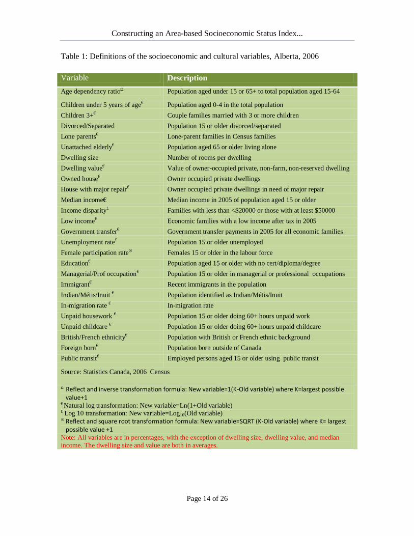
the present study is provided in Table 110

.

Assessing Outliers, Normality, and Linearity

A number of issues need to be considered when attempting a factor analysis (Nardo,

Saisana, Saltelli, & Tarantola, 2005). These assumptions are discussed in almost all

statistical textbooks and SPSS manuals, but are often neglected by researchers when they

develop composite indices, based on factor/principal components analyses. Although

sample size, variable scaling (interval vs. categorical), and relevancy of sub-indicators

that measure underlying dimensions are important assumptions in the application of

factor/principal components analyses, they are not discussed here because none of these

assumptions pertain to our data. More specifically, all variables were measured at the

interval-level and only the relevant variables were included in the correlation matrix.

Further, regardless of the fact that there are no scientific answer on the question of how

10 The initial selection included 42 variables in total. In some instances, different computations of the same

variable, were considered to avoid a large number of missing cases and/or extreme values. For example,

‘proportion of all couples with 3 or more children’ and ‘proportion of married couples with 3 or more

children’ were both computed, but only the second variable was retained. A complete list of variables that

were considered are available upon request.


Page 13 of 26

many cases are necessary, our sample size satisfied both the cases-to-variables ratio and

the rule of 200, as endorsed by Bryant & Yarmold (1995) (see, Nardo, Saisana, Saltelli,

& Tarantola, 2005).

As with most statistical techniques, the presence of outliers can affect factor analysis

results and their interpretations; outliers or values that are substantially lower or higher

than the other values in the data set can impact correlations and thus distort factor

analysis. They were checked using various SPSS procedures, such as the histogram or the

actual shape of the distribution, normal Q-Q plot where the observed value for each

score is plotted against the expected value, the box-plot of the distribution of scores, and

the descriptive statistics, such as mean and 5% trimmed mean (Table 2).11 Outliers were

detected in all variables and were removed before performing factor analysis.

Second, factor analysis can be sensitive to non-linear relationship where the two variables

are related in a non-linear fashion. If this occurs, the correlation coefficient can

underestimate the strength of the relationship. The problem can be critical, especially

when dealing with small samples. All variables, with the exception of six variables -

percentage of those aged 15 or older divorced/separated, dwelling size, median income,

female participation rate, percentage aged 15 or older with no certificate/diploma/degree,

percentage of immigrants in the population, percentage of population with British/French

ethnic background, and percentage of employed persons aged 15 or older using a public

transit - were transformed statistically, using reflect and inverse, reflect and square root,

natural logarithm or log10, depending upon the nature or skewness of the distribution. The

trimmed mean and mean values were found very similar after transformation, indicating

that there is no cause for concern in terms of extreme cases (Table 2).

In addition, descriptive statistics, such as skewness (a measure of symmetry), and kurtosis

(a measure of ‘peakedness’) can be used to detect the type of distribution. The results

showed extremely small positive or negative values, providing a further validation of

symmetry.12

Finally, another test of normality was done by inspecting the Kolmogorow-

Smirnov statistic, the results of which are presented on Table 3. A significant result

(0.00), suggests no violation of the assumption of normality.

11 In SPSS, the outliers are points that lay more than 1.5 box-lengths from the edge of the box. 12 In a large sample situation, as Tabachnick & Fidell (2007) noted, skewness “will not make a

substantive difference” (p. 80). Kurtosis can result in an underestimate of the variance, but this will also be taken care of, if the sample size is large (200+ cases). Despite having a large sample

size, we inspected the shape of the distribution.


Page 14 of 26

Table 1: Definitions of the socioeconomic and cultural variables, Alberta, 2006

Variable Description

Age dependency ratioΩ Population aged under 15 or 65+ to total population aged 15-64

Children under 5 years of age€ Population aged 0-4 in the total population

Children 3+€ Couple families married with 3 or more children

Divorced/Separated Population 15 or older divorced/separated

Lone parents€ Lone-parent families in Census families

Unattached elderly€ Population aged 65 or older living alone

Dwelling size Number of rooms per dwelling

Dwelling value€ Value of owner-occupied private, non-farm, non-reserved dwelling

Owned house€ Owner occupied private dwellings

House with major repair€ Owner occupied private dwellings in need of major repair

Median income€ Median income in 2005 of population aged 15 or older

Income disparity£ Families with less than <$20000 or those with at least $50000

Low income€ Economic families with a low income after tax in 2005

Government transfer€ Government transfer payments in 2005 for all economic families

Unemployment rate£ Population 15 or older unemployed

Female participation rate Females 15 or older in the labour force

Education€ Population aged 15 or older with no cert/diploma/degree

Managerial/Prof occupation€ Population 15 or older in managerial or professional occupations

Immigrant€ Recent immigrants in the population

Indian/Métis/Inuit € Population identified as Indian/Métis/Inuit

In-migration rate € In-migration rate

Unpaid housework € Population 15 or older doing 60+ hours unpaid work

Unpaid childcare € Population 15 or older doing 60+ hours unpaid childcare

British/French ethnicity€ Population with British or French ethnic background

Foreign born€ Population born outside of Canada

Public transit€ Employed persons aged 15 or older using public transit

Source: Statistics Canada, 2006 Census

Ω Reflect and inverse transformation formula: New variable=1(K-Old variable) where K=largest possible

value+1 € Natural log transformation: New variable=Ln(1+Old variable) £ Log 10 transformation: New variable=Log10(Old variable) Reflect and square root transformation formula: New variable=SQRT (K-Old variable) where K= largest

possible value +1 Note: All variables are in percentages, with the exception of dwelling size, dwelling value, and median

income. The dwelling size and value are both in averages.


Page 15 of 26

Testing the Appropriateness of a Factor Analysis

Before being submitted to a factor analysis, the correlations were checked for

multicollinearity problems. Some researchers use factor analysis if the variables show

multicollinearity. However, multicollinearity could increase the standard error of factor

loadings, making them less reliable and also difficult to label. Some researchers, either

combine collinear variables or eliminate them prior to factor analysis. Some others forgo

factor analysis altogether. In the present study, the Kaiser-Meyer-Olkin (KMO), a

Measure of Sampling Adequacy (MSA) was used to detect multicollinearity in the data so

that the appropriateness of carrying out a factor analysis can be detected. More

specifically, sampling adequacy predicts if data are likely to factor well, based on

correlations and partial correlations. The KMO measure compares the magnitudes of the

observed correlation coefficients to the magnitudes of the partial correlation coefficients.

If the variables, in fact, have common factors, the partial correlation coefficients should

be small relative to the total correlation coefficient. The maximum value of KMO can be

1.0, a value of 0.9 is considered as ‘marvelous’, 0.80, ‘meritorious’, 0.70, ‘middling’,

0.60, ‘mediocre’, 0.50, ‘miserable’ (Antony & Rao, 2007; see also, Planning

Commission, 1993). For our data, it was 0.857, signaling that a factor analysis of the

variables can proceed (Table 3).

Table 2: Descriptive statistics of the socioeconomic and cultural variablesΩ

Variable Mean 5% Trimmed

Mean Skewness Kurtosis Range

Age dependency ratio 4.40 4.32 0.35 -0.68 8.92

Children under 5 years of age 1.85 1.86 -0.25 0.29 2.42

Children 3+ 2.48 2.48 -0.24 -0.20 2.69

Divorced/Separated 2.38 2.40 -0.52 0.21 2.64

Lone parents 2.76 2.76 0.02 -0.62 2.77

Unattached elderly 3.44 3.43 -0.08 -0.44 2.63

Dwelling size 7.05 7.07 -0.26 0.90 2.15

Dwelling value 12.43 12.43 0.15 0.60 3.22

Owned house 4.27 4.33 -2.52 7.51 3.38

House with major repair 2.26 2.25 0.36 0.68 3.95

Median income 10.25 10.25 -0.26 0.90 2.15

Income disparity 0.21 0.19 0.65 0.78 2.05

Low income 2.48 2.46 -0.45 -0.17 3.04

Government transfer 2.13 2.14 -0.23 -0.07 3.71

Unemployment rate 0.70 0.70 0.61 0.85 1.55

Female participation rate 5.73 5.73 0.03 0.24 7.65

Education 3.14 3.16 -0.52 0.46 3.26

Managerial/Professional occupation 2.82 2.83 -0.24 -0.42 2.97

Immigrant 1.70 1.67 0.60 -0.39 3.13


Page 16 of 26

Indian/Métis/Inuit 1.84 1.78 1.18 1.94 4.12

In- migration rate 3.67 3.69 -0.37 -0.46 3.39

Unpaid housework 1.78 1.76 0.60 0.27 3.20

Unpaid childcare 2.14 2.15 -0.07 -0.23 3.08

British/French ethnicity 3.63 3.66 -3.21 15.97 3.15

Foreign born 2.58 2.59 -0.18 -0.77 3.32

Public transit 2.51 2.52 -0.38 -0.56 3.29

Ω The statistics are based on the transformed variables when a transformation was required.

Another test of the strength of the relationship among variables was done using the

Bartlett’s (1954) Test of Sphericity. The Bartlett’s Test of Sphericity tests the null

hypothesis that the variables in the population correlation matrix are uncorrelated. The

results of our analysis showed a significance level of 0.00, a value that is small enough to

reject the hypothesis (the probability should be less than 0.05 to reject the null). It can be

concluded that the strength of the relationship among variables is strong or the correlation

matrix is not an identity matrix as is required by factor analysis to be valid. These

diagnostic procedures indicate that factor analysis is appropriate for the data.

Table 3: KMO measure of sampling adequacy and Bartlett's test of sphericity

KMO Measure of

Sampling Adequacy

Bartlett's Test of Sphericity

Chi-Square df Sig

0.857 17087.394 325 0.00

Interpretation of Results from PCA

The 26 variables were included in the factor analysis. Because the variables were not

standardized, the correlation matrix was used as an input to PCA to extract the factors. 13

The results are presented in Table 4. The number of factors extracted can be defined by

the user, and there are techniques available in SPSS that can be used to help decide the

number of factors. One of the most commonly used techniques is Kaiser’s criterion, or

the eigenvalue rule. Under this rule, only those factors with an eigenvalue (the variances

extracted by the factors) of 1.0 or more are retained. Using this criterion, our data

revealed 8 factors.

13 When PCA is used, we have the option of using either the correlation or the covariance matrix.

Because PCA is sensitive to differences in the units of measurement of variables, it is useful to

standardize the variables before applying PCA (Bolch & Huang, 1974). However, since the correlation matrix is the standardized version of the covariance matrix, a correlation matrix

should be used, if standardization of variables was not done.


Page 17 of 26

For the present study, we also used a graphical method, known as the Catell’s (1966)

scree test (Figure 2). These are plots of each of the eigenvalues of the factors. One can

inspect the plot to find the place where the smooth decrease of eigenvalues appears to

level off. To the right of this point, only ‘factorial scree’ (meaning debris which collects

on the lower part of a rocky slope) is found. After examining the screeplot, only five

factors were extracted for analysis.

The results of PCA using varimax rotation are presented in Table 4. Five factors

accounted for 55.7 per cent of the total variance in the data. For the first factor, income

disparity, government transfer payments, and education showed markedly higher positive

loadings, while dwelling value, median income, and occupation showed strong negative

factor loadings. Loading resulting from an orthogonal rotation are correlation coefficients

of each variable with the factor, so they naturally range from -1 to +1. A negative loading

simply means that the results need to be interpreted in the opposite direction from the

way it is worded. Higher value of housing in the original data indicate better

socioeconomic circumstances, hence the negative sign on this variable means a higher

economic situation. The first factor accounted for 16.3 per cent of the total variation. This

factor is a reasonable representation of the economic system. It means that better

economic circumstances are associated with high dwelling value, high median income,

and high percentage of population in managerial/professional occupations, and low

income disparity, low government transfer payments, and low percentage of population

with higher education.

Figure 2: Screeplot of eigenvalues of factors


Page 18 of 26

For the second factor, age dependency ratio, divorced/separated, unattached elderly, lone

parents, and low income showed strong positive loadings and dwelling size and owned

house showed strong negative loadings. The second factor accounted for 14.7 per cent of

the variance. We may interpret this factor as a measure of the social system. The third

factor accounted for 9.2 per cent of the variations and explains the variations in

British/French ethnicity, recent immigrants, in-migration rate, foreign-born population,

and public transit. This factor is a measure of the cultural system because four out of the

five cultural variables load high on this factor. The fourth factor accounted for 8.9 per

cent of the variance and explains the variations in house with major repair,

Indian/Métis/Inuit, unemployment rate, unpaid housework, and couples with three or

more children. The interpretation of this factor or the labeling of it is less straightforward;

however, it is representative of vulnerable group membership. The fifth factor accounted

for 6.7 per cent of the variance explaining the differences in children under age five and

unpaid child care, and female labor force participation. The study by Fukuda, Nakamura,

& Takano (2007) in Japan found similar negative loadings for variables, dwelling size,

income, and owned houses and positive loadings for unemployment rate and aged single

dwellings in their study.

Table 4: Results of PCA: Varimax rotation factor matrix

Variable Factor

1

Factor

2

Factor

3

Factor

4

Factor

5

Age Dependency ratio 0.839

Children under 5 years of age 0.782

Children 3+ 0.437

Divorced/Separated 0.653

Lone parents 0.518

Unattached elderly 0.579

Dwelling Size -0.768

Dwelling value -0.738

Owned house -0.810

House with major repair 0.629

Median income -0.726

Income disparity 0.734

Low income 0.491

Government transfer 0.843

Unemployment rate 0.570

Female participation rate -0.478

Education 0.748

Managerial/Professional Occupation

-0.694

Immigrant 0.573

Indian/Métis/Inuit 0.629

In-migration rate -0.464


Page 19 of 26

Unpaid housework 0.555

Unpaid childcare 0.699

British/French ethnicity -0.647

Foreign born 0.804

Public transit 0.472

Percent of variance (55.69%) 16.25% 14.68% 9.15% 8.92% 6.69%

Note: A variable with a positive loading indicates a negative association to the component.

Calculating the Socioeconomic Index

As a first step in the computation of a single index, factor score coefficients, also called

component scores were estimated using regression method. Factor scores are the scores

of each case (DA, in our example), on each factor. To compute the factor scores for a

given case for a given factor, the case’s standardized score on each variable is multiplied

by the corresponding factor loading of the variable for the given factor, and summed

these products. This calculation was carried out using SPSS procedure and factor scores

were saved as variables in subsequent calculations involving factor scores.

The five factors explained 55.7 per cent of the total variation, with the first, second, third,

fourth, and fifth factors, explaining 16.3 per cent, 14.7 per cent, 9.2 per cent, 8.9 per cent,

and 6.7 per cent respectively. Therefore, the importance of the factors in measuring

overall socioeconomic condition is not the same. Using the proportion of these

percentages as weights on the factor score coefficients, a Non- standardized Index (NSI)

was developed for each DA, using the formula:

NSI = (16.25/55.69) (Factor 1 score) + (14.68/55.69) (Factor 2 score) + (9.15/55.69) (Factor 3

score) + (8.92/55.69) (Factor 4 score) + (6.69/55.69) (Factor 5 score)

This index measures the socioeconomic status of one DA relative to the other on a linear

scale. The value of the index can be positive or negative, making it difficult to interpret.

Therefore, a Standardized Index (SI) was developed, the value of which can range from 0

to 100, using the formula:

SI=

SI=

A similar procedure was adopted in previous research (Antony & Rao, 2007; Hightower,

1978; Sekhar, Indrayan, & Gupta, 1991). The scores were later reversed to make the

interpretation easier; the higher the value, the better the socioeconomic status of an area.


Page 20 of 26

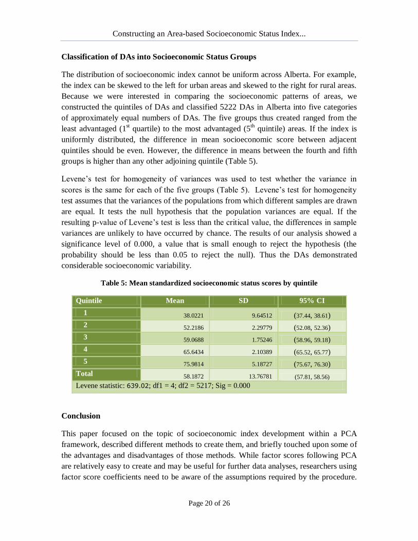
Classification of DAs into Socioeconomic Status Groups

The distribution of socioeconomic index cannot be uniform across Alberta. For example,

the index can be skewed to the left for urban areas and skewed to the right for rural areas.

Because we were interested in comparing the socioeconomic patterns of areas, we

constructed the quintiles of DAs and classified 5222 DAs in Alberta into five categories

of approximately equal numbers of DAs. The five groups thus created ranged from the

least advantaged (1st quartile) to the most advantaged (5

th quintile) areas. If the index is

uniformly distributed, the difference in mean socioeconomic score between adjacent

quintiles should be even. However, the difference in means between the fourth and fifth

groups is higher than any other adjoining quintile (Table 5).

Levene’s test for homogeneity of variances was used to test whether the variance in

scores is the same for each of the five groups (Table 5). Levene’s test for homogeneity

test assumes that the variances of the populations from which different samples are drawn

are equal. It tests the null hypothesis that the population variances are equal. If the

resulting p-value of Levene’s test is less than the critical value, the differences in sample

variances are unlikely to have occurred by chance. The results of our analysis showed a

significance level of 0.000, a value that is small enough to reject the hypothesis (the

probability should be less than 0.05 to reject the null). Thus the DAs demonstrated

considerable socioeconomic variability.

Table 5: Mean standardized socioeconomic status scores by quintile

Quintile Mean SD 95% CI

1 38.0221 9.64512 (37.44, 38.61)

2 52.2186 2.29779 (52.08, 52.36)

3 59.0688 1.75246 (58.96, 59.18)

4 65.6434 2.10389 (65.52, 65.77)

5 75.9814 5.18727 (75.67, 76.30)

Total 58.1872 13.76781 (57.81, 58.56)

Levene statistic: 639.02; df1 = 4; df2 = 5217; Sig = 0.000

Conclusion

This paper focused on the topic of socioeconomic index development within a PCA

framework, described different methods to create them, and briefly touched upon some of

the advantages and disadvantages of those methods. While factor scores following PCA

are relatively easy to create and may be useful for further data analyses, researchers using

factor score coefficients need to be aware of the assumptions required by the procedure.


Page 21 of 26

While data screening and checking assumptions for outliers, normality, linearity, and

homoscedasticity are part of most parametric tests, they need to be revisited in the context

of factor analysis because they can determine whether or not a particular data set is

suitable for factor analysis. For example, factor scores may be skewed or non-normal,

especially if the factorability of the correlation matrix as suggested by Bartlett’s Test of

Sphericity does not reach statistical significance. Clearly, there are methodological issues

related to data quality that need to be addressed when developing PCA-based indices.

The multi-dimensional composite index developed here within the framework of PCA

provides a better picture of economic, social, cultural, and related structural conditions,

and thereby, socioeconomic stratification of areas across major socioeconomic groupings,

such as quintiles. The differences in mean socioeconomic scores were found uneven in

Alberta, across socioeconomic categories at the small area level; the mean difference in

socioeconomic index is higher between the fourth and richest quintiles than any other

adjacent quintiles. However, researchers need to be cautioned about interpreting the

results. First, the socioeconomic scores should not be generalized to those based on

individual-level data. Second, socioeconomic groupings are obtained by classifying

Dissemination Areas and ranking the scores prior to grouping. The index provides only a

relative measure of inequality between areas, and it cannot provide information on

absolute levels of economic, social, or cultural aspects within a community. It can be

used for comparisons across areas, or over time, provided the computational procedures

follow the same method and same set of variables. Finally, the index came from the

correlations in the data for Alberta. The construction of an index at the community-level

can risk our effort to capture urban-rural disparities. For example, in urban areas,

property and housing value may emerge as important variables whereas in rural areas,

family size or accessibility to services may emerge as important. In the absence of

individual socioeconomic data on relevant variables, area measures such as the one

developed here may be extremely useful for the purposes of monitoring disparities in

health and developmental outcomes (e.g., infant mortality, cancer mortality, Early Child

Development instrument (EDI)) and for identifying communities that may be targeted for

programs to improve access to services or infrastructure development and also specific

interventions to improve overall quality of life and welfare (Krishnan, 2010).

The choice of variables included can have an impact on the index, thereby influencing

health outcomes, such as early child development. For example, Houweling, Kunst, &

Mackenbach (2003) noted the classification of socioeconomic groups as impacting child

health outcomes, directly. Variables or their proxies require careful consideration,

especially when socioeconomic indices are used as determinants of health outcomes.

Further, variables such as, durable assets (collected locally) and population density might

prove to be important correlates of socioeconomic inequalities. In any case,

socioeconomic status indicators, which vary by individuals, locations, or times, should


Page 22 of 26

take into account the complex nature and also the bio-ecological aspects of health

outcomes.

Acknowledgement

I am indebted to my colleagues and support staff, in particular Dr. Susan Lynch (Director,

ECMap), for her support, encouragement and helpful comments throughout the course of

this project. I would also like to thank Olenka Melnyk for her comments on an earlier

version of the manuscript.


Page 23 of 26

References

Antony, G. M. & Rao, K. V. (2007). A composite index to explain variations in poverty,

health, nutritional status and standard of living: Use of multivariate statistical

methods. Public Health, 121, 578-587.

Ackerman, B. P. & Brown, E. D. (2010). Physical and psychological turmoil in the home

and cognitive development. In G. W. Evans & T. D. Wachs (Eds.), Chaos and its

Influence on Children’s Development (pp. 35-47). Washington, DC: American

Psychological Association.

Bartlett, M. S. (1954). A note on the multiplying factors for various chi square

approximations. Journal of the Royal Statistical Society, 16 (Series B), 296-8.

Boelhouwer, J. & Stoop, I. (1999). Measuring well-being in the Netherlands: The SCP

index from 1974 to 1997. Social Indicators Research, 48(1), 51-75.

Bolch, B. W. & Huang, C. J. (1974). Multivariate Statistical Methods for Business and

Economics. Englewood Cliffs, NJ: Prentice Hall.

Braveman, P. A., Cubbin, C., Egerter, S., Chideya, S., Marchi, K. S., Metzier, M., Fosner,

S. (2005). Socioeconomic status in health research: One size does not fit all. The

Journal of American Medical Association, 294, 2879-2888

British Columbia (2009). British Columbia Regional Socio-Economic Indicators:

Methodology, British Columbia: Ministry of Labor & Citizens Services.

Canadian Institute for Health Information (2005). Developing a healthy community’s

index: A collection of papers.

Catell, R. B. (1966). The scree test for numbers of factors. Multivariate Behavioral

Research, 1, 245-76.

Crosnoe, R. (2007). Early child care and the school readiness of children from Mexican

immigrant families. IMR (Spring), 41(1), 152-181.

Cubbin, C., LeClere, F., & Smith, G. (2000). Socioeconomic status and injury mortality:

Individual and neighborhood determinants. Journal of Epidemiology and

Community Health, 54, 517-524.

Davey, S. M. & Hart, C. (1999). Use of census-based aggregate variables to proxy for

socioeconomic group: evidence from national samples. American Journal of

Epidemiology, 150(9), 996-7.

Davis, P., McLeod, K., Ransom, M., Ongley, P., Pearce, N., & Howden-Chapman, P.

(1999). The New Zealand Socioeconomic Index: Developing and validating an

occupationally-derived indicator of socioeconomic status. Australian and New

Zealand Journal of Public Health, 23(1), 27-33.

Diez-Roux, A. V. (2003). Residential environments and cardiovascular risk. Journal of

Urban Health, 80(4), 569-589.

Eibner, C., & Sturm, R. (2006). US-based indices of area-level deprivation: Results from

health care for communities. Social Science & Medicine, 62(2), 348-359.

Evans, G. W. (2004). The environment of childhood poverty. American Psychologist, 59,

77-92.

Evans, G. W. (2006). Child development and the physical environment. Annual Review of

Psychology, 57, 423-451.


Page 24 of 26

Evans, G. W. & Wachs, T. D. (2010) (Eds.), Chaos and its Influence on Children’s

Development. Washington, DC: American Psychological Association.

Fukuda, Y., Nakamura, K., & Takano, T (2007). Higher mortality in areas of lower

socioeconomic position measured by a single index of deprivation in Japan. Public

Health, 121, 163-173.

Fotso, J. & Kuate-defo, B. (2005). Measuring socioeconomic status in health research in

developing countries: Should we be focusing on households, communities, or both?

Social Indicators Research, 72, 189-237.

Geronimus, A. T., & Bound, J. (1998). Use of census-based aggregate variables to proxy

for socioeconomic group: evidence from national samples. American Journal of


Gilthorpe, M. S. (1995). The importance of normalization in the construction of

deprivation indices. Journal of Epidemiology and Community Health, 49

(Supplement 2), S45-S50.

Gjolberg, M. (2009). Measuring the immeasurable? Constructing an index of CSR

practices and CSR performance in 20 countries. Scandinavian Journal of

Management, 25, 10-22.

Havard, S., Deguen, S., Bodin, J., Louis, K., & Laurent, O. (2008). A small-area index of

socioeconomic deprivation to capture health inequalities in France. Social Science

& Medicine, 67, 2007-2016.

Hightower, W. L. (1978). Development of an index of health utilizing factor analysis.

Medical Care, 16, 245-55.

Houweling, T. A. J., Kunst, A. E., & Mackenbach, J. P. (2003). Measuring health

inequality among children in developing countries: does the choice of the indicator

of socioeconomic status matter? International Journal for Equity in Health, 2, 8. Kershaw, P., Irwin, L., Trafford, K., & Hertzman, C. (2005). The British Columbia Atlas

of Child Development (Volume 40), Human Early Learning Partnership, Western

Geographical Press.

Krishnan, V. (2010). Early child development: A conceptual model. Presented at the

Early Childhood Council Annual Conference 2010, Christchurch, New Zealand, 7

May, 2010.

Lai, D. (2003). Principal component analysis on human development indicators of China.

Social Indicators Research, 61(3), 319-330.

Liu, X & Lu, K. (2008). Student performance and family socioeconomic status. Chinese

Education and Society, 41(5), 70-83.

Lustig, S. L. (2010). An ecological framework for the refugee experience: What is the

impact on child development? In G. W. Evans & T. D. Wachs (Eds.), Chaos and its

Influence on Children’s Development (pp. 239-251). Washington, DC: American

Psychological Association.


Page 25 of 26

Markides, K. S. & McFarland, C. (1982). A note on recent trends in the infant mortality-

socioeconomic status relationship. Social Forces, 61(1), 268-276.

Messer, L. C., Vinikoor, L. C., Laraia, B. A., Kaufman, J. S., Eyster, J., Holzman, C.,

Culhane, J., Elo, I., Burke, J. G., & O’Campo, P. (2008). Socioeconomic domains

and associations with preterm birth. Social Science & Medicine, 67, 1247-1257.

Morris, R. & Castairs, V. (1991). Which deprivation? A comparison of selected

deprivation indices. Journal of Public Health Medicine, 13, 318-326.

Mustard, C. A., Derksen, S., Berthelot, J. M., & Wolfson, M. (1999). Assessing ecologic

proxies for household income: a comparison of household and neighborhood level

income measures in the study of population health status. Health and Place, 5(2),

157-71.

Nardo, M., Saisano, M., Saltelli, A., & Tarantola, S. (2005). Tools for Composite

Indicators Building. Italy: European Commission Joint Research Centre, Institute

for the Protection and Security of the Citizen Econometrics and Statistical Support

to Antifraud Unit

Oakes, J. M. & Rossi, P. H. (2003). The measurement of SES in health research: Current

practice and steps toward a new approach. Social Science & Medicine, 56(4), 769-

784.

Pallant, J. (2007), SPSS Survival Manual: A Step by Step Guide to Data Analysis Using

SPSS for Windows (3rd

edition). New York: McGraw Hill, Open University Press.

Pampalon, R., & Raymond, G. (2000). A deprivation index for health and welfare

planning in Quebec. Chronic Diseases in Canada, 21, 104-113.

Pampalon, R., Hamel, D., & Gamache, P. (2009). A comparison of individual and area-

based socioeconomic data for monitoring social inequalities in health (Statistics

Canada, Catalogue no. 82-003-XPE). Health Reports, 20(3) (September), 85-94.

Pearson, K. (1901). On Lines and Planes of Closest Fit to Systems of Points in Space

Philosophical Magazine 2 (6),559–572.

Perreira, K. M. & Smith, L. (2007). A cultural-ecological model of migration and

development: Focusing on Latino immigrant youth. The Prevention Researcher,

14(4), 6-9.

Planning Commission (1993). Report on the Expert Group on Estimation of Proportion

and Number of Poor, New Delhi: Perspective Planning Division.

Program Effectiveness Data Analysis Coordinators of Eastern Ontario (2009). Early

Childhood Risks, Resources, and Outcomes in Ottawa

(http://parentresource.on.ca/DACSI_ e.html). Ottawa: Parent Resource Centre.

Reed, B. A., Habicht, J.P., & Niameogo, C. (1996). The effects of maternal education on

child nutritional status depend on socio-environmental conditions. International

Journal of Epidemiology, 25, 585-592.

Rygel, L., O’Sullivan, D. & Yarnal, B. (2006). A method for constructing a social

vulnerability index: An application to hurricane storm surges in a developed

country. Migration and Adaptation Strategies for Global Change, 11, 741-764.

http://stat.smmu.edu.cn/history/pearson1901.pdf

http://parentresource.on.ca/DACSI_%20e.html


Page 26 of 26

Saltelli, A., Nardo, M., Saisana, M., & Tarantola, S. (2004). Composite indicators-The

controversy and the way forward, OECD World Forum on Key Indicators, Palermo,

10-13 November.

Sekhar, C. C., Indrayan, A., & Gupta, S. M. (1991). International Journal of


Shavers, V. L. (2007). Measurement of socioeconomic status in health disparities

research. Journal of the National Medical Association, 99(9), 1013-1023.

Shevky, E. & Bell, W. (1955). Social Area Analysis. Stanford: Stanford University Press.

Singh, G. K., Miller, B. A., & Hankey, B. F. (2002). Changing area socioeconomic

patterns in U.S. cancer mortality, 1950-1998: Part II-Lung and colorectal cancers.

Journal of the National Cancer Institute, 94(12), 916-925.

Steenland, K., Henley, J., Calle, E., & Thun, M. (2004). Individual-and area-based

socioeconomic status variables as predictors of mortality in a cohort of 179,383

persons. American Journal of Epidemiology, 159(11), 1047-1056.

Subramanian, S. V., Chen, J. T., Rehkopf, D. H., Waterman, P. D., & Krieger, N. (2006).

Comparing individual and area-based socioeconomic measures for the surveillance

of health disparities: A multilevel analysis of Massachusetts births, 1989-1991.

American Journal of Epidemiology, 164(9), 823-34.

Tabachnick, B. G., & Fedell, L. S. (2007). Using Multivariate Statistics (5th

edition).

Boston: Pearson Education.

Tata, R. J. & Schultz, R. R. (1988). World variation in human welfare: A new index of

development status. Annals of the Association of American Geographers, 78(4),

580-593.

Vyas, S. & Kumaranayake, L. (2006). Constructing socioeconomic status indices: How to

use principal components analysis. Advance Access Publication, 9, 459-468.

Zagorski, K. (1985). Composite measures of social, economic, and demographic regional

differentiation in Australia: Application of multi-stage principal component

methods to aggregate data analysis. Social Indicators Research, 16, 131-156.

Documents

Constructing an Area-based Socioeconomic Index: A ... · Constructing an Area-based Socioeconomic Index: ... but also helps to design theories and conceptual frameworks of a ... means