COMPUTATIONAL FLUID DYNAMICS MODEL FOR … · COMPUTATIONAL FLUID DYNAMICS MODEL FOR TACOMA NARROWS BRIDGE UPGRADE PROJECT ... The commercial CFD code, AcuSolve, was chosen for the

1 Copyright © #### by ASME

Proceedings of FEDSM’03: 4TH ASME.JSME JOINT FLUIDS ENGINEERING CONFERENCE

July 6-11, 2003 - Honolulu, Hawaii

FEDSM2003-45514

COMPUTATIONAL FLUID DYNAMICS MODEL FOR TACOMA NARROWS BRIDGE UPGRADE PROJECT

Kristian Debus, Jonathan Berkoe, Brigette Rosendall

Bechtel National Inc., P.O. Box 193965, San Francisco, California 94119-3965

Farzin Shakib ACUSIM Software, Inc., 2685 Marine Way, Suite 1215,

Mountain View, California 94043

ABSTRACT

The purpose of this work was to validate and apply a commercial computational fluid dynamics code with a hybrid RANS/LES turbulence computational model for a flow past a bluff body ultimately to help in the design of the caisson anchoring system during construction of a new adjacent span of the Tacoma Narrows Bridge. INTRODUCTION

The new Tacoma Narrows Bridge will be designed as a suspension bridge and operated parallel to the existing Tacoma Narrows crossing in Tacoma, Washington (see Figure 1). This is the largest suspension bridge built in the USA in the last 40 years, and the first time a major suspension bridge has been constructed parallel and so near to an existing bridge.

Fig. 1 Rendering of future new span (shown on left)

of Tacoma Narrows Bridge Tacoma Narrows Constructors has commissioned a study

involving the use of CFD modeling in support of the Tacoma Narrows Bridge Expansion Project. During the construction

of the new caissons a complex, cable-supported anchoring system will be used to control the positions of the caissons located 65 feet from the existing bridge piers. During installation, the caissons will be subjected to current-driven loads and vortex shedding. The CFD model results for the East and West pier configurations will provide input data to the dynamic mooring analysis of the flow-structure interactions to determine the expected and maximum forces on the anchoring system cables.

CFD is an especially important tool in this case due to the lack of relevant field measurement data for similar structures or experimental scale model data for similar configurations.

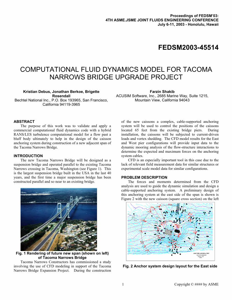
PROBLEM DESCRIPTION The forces and moments determined from the CFD

analysis are used to guide the dynamic simulation and design a cable-supported anchoring system. A preliminary design of this anchoring system at the east side of the span is shown is Figure 2 with the new caisson (square cross section) on the left

Fig. 2 Anchor system design layout for the East side


and the existing pier on the right. The anchor positions are indicated by the dots and are distributed around the caissons. Positioning of the anchors and attached cables is based on the expected current-induced load distribution during installation, installation logistics, riverbed soil considerations, and water depth. Additionally and of critical importance, it has been stipulated that the existing bridge structure cannot be touched by any of the anchors or cables. This results in a very complex design procedure that will be unique for each side of the span.

Since the Tacoma Narrows is a tidal channel, the current flow cycles through opposing directions, referred to as flood and ebb. During flood conditions maximum flow speeds of 9 knots (4.6 m/s) at the East piers and 7 knots (3.6 m/s) at the West piers can occur. In the ebb direction the maximum velocity for both sides is around 7 knots (3.6 m/s). For flood direction, the caisson is positioned in the wake of the pier where the effects of vortex shedding prevail; for the ebb direction, the upstream caisson is subjected primarily to drag forces.

In summary, the key technical challenges for this analysis are as follows:

• The transverse loads on the caisson – particularly during the flood flow direction scenario in which the caisson lies in the wake of the existing pier – are significant and may critically affect the stability of the structure. These loads are induced by the current flow adjacent to the caisson and also by the shedding and subsequent flow recirculation of vortices in the wake region. The vortex shedding phenomena is explicitly transient (time-varying) and unsteady (see Figure 3).

• The Reynolds number of the flow around the piers is on the order of 108 (100 million). No literature has been found applying CFD in this range of Reynolds number. The implication of the high Reynolds number is the difficulty in predicting the flow separation points and vortex shedding frequencies in the wake regions.

• It has been observed at the existing bridge that the vortices shed from the pier are directed downward. It is also believed that the downward direction to the vortices is coupled to the transverse components of the vortex formation.

Fig. 3 Complex flow structures in the wake region of the existing pier (east side) at Tacoma Narrows

These considerations necessitated the development of a fully three-dimensional modeling approach. The commercial CFD code, AcuSolve, was chosen for the model because its equal-order pressure/velocity coupling results in fast convergence and was developed to run very efficiently on parallel platforms. Also, the hybrid RANS/LES turbulence model is the most appropriate choice for high Reynolds number flows around bluff bodies. By using this methodology it was possible to achieve excellent accuracy with relatively fast solution times.

CFD MODEL DESCRIPTION

Solution Methodology AcuSolve solves the transient turbulent incompressible

Navier-Stokes equations

τρ ⋅∇+−∇=

=⋅∇

pDtDuu 0

These are, respectively, the conservation of mass and momentum in three-dimensions. Here ∇⋅+∂∂= utDtD // is the material derivative; u is the velocity vector; ρ is the density; p is the pressure; and τ is the stress tensor which is the sum of contributions from the viscous and turbulence Reynolds stress, modeled as

))(( uu Tt ∇+∇+= µµτ

where µ and tµ are, respectively, the molecular and turbulent eddy viscosities.

The one-equation Spalart-Allmaras (SA) RANS turbulence model with the Detached-Eddy Simulation (DES) modification is used to model the eddy-viscosity. The SA RANS model may be written as

( )2

12

21

~)~(~)~(1~~~

−∇+∇+⋅∇+=

dfccSc

DtD

wwbbννννν

σνν

Where ν~ is the unknown field; see [Spalart 92] for details and

definition of S~ and wf and constantsσ , 1bc , 2bc , and 1wc . ν~ is closely related to kinematic eddy viscosity. The turbulence eddy viscosity is then given by

µνρχχ

χνρµ /~ ~31

3

3

=+

=v

t c

The DES model is obtained by replacing the distance to the nearest wall, d , by

),min(~∆= DESCdd

Here ∆ is a local measure of element size and DESC is a constant; see [Spalart 97] for details.

It is well known that RANS turbulence models can be very effective in resolving boundary layers and free-stream flows. However, they do a poor job in capturing free shears. On the other hand, LES turbulence models can be effective in capturing the free shear, while they need unattainable mesh resolution to capture boundary layers, especially at high Reynolds numbers. For well-generated meshes, DES is


designed to naturally switch between RANS and LES where appropriate. The mesh spacing in the boundary layers is of the order of boundary layer thickness. Consequently, in the boundary layer, DES reverts to the “RANS mode” to predict the boundary layer and flow separations. Away from the walls, and when production and destruction terms are balanced, the length scale ∆= DESCd~ of the model yields a Smagorinsky

LES eddy viscosity 2~ ∆∝ Sν . In short, DES attempts to provide the best of both worlds.

The above equations constitute a system of five equations with five unknowns. These equations are solved using the Galerkin/Least-Squares finite element technology; see [Hughes 87] and references therein for in-depth description.

Equal-order nodal interpolations for all working variables, including pressure, are used with low-order elements. Moreover, the semi-discrete generalized-α method of [Hulbert 93] is used to resolve the time dependencies.

The Galerkin finite element formulation provides the base algorithm. Galerkin formulation, which is equivalent to central-difference formulation in finite differences, does not yield stable discretization for the solution of the incompressible Navier-Stokes equations. The stability difficulties arise from two main sources: (1) the divergence-free constraint, i.e., the continuity equation; and (2) the convective term in the momentum equations. The least-squares operator is designed to add the needed stability without sacrificing accuracy.

AcuSolve improves performance in three ways: (1) it solves the coupled velocity/pressure system, yielding substantially faster convergence; (2) its architecture has been implemented from the ground up for vector and cache-based super-scalar machines; (3) it is designed for coarse-grain parallel machines. Domain decomposition is used to break and distribute the elements and nodes to different processors. Message Passing Interface (MPI) is used to communicate between the processors. All the algorithms are designed specifically to perform on coarse-grain parallel machines.

Model Geometry and Bathymetry The CFD model was set up as a rigid body system

submerged in water. The complex bathymetry (based on actual mapping of the riverbed) was imported to the meshing tool from a CAD model. The bathymetry data was converted using Microstation (Bentley, Inc.) to a surface model suitable for export to the CFD meshing software. Separate models were created for the East and West piers. Each of these models extended sufficient distance into the channel to allow for specification of far-field boundary condition.

Fig. 4 Computational domain for the west side with

bathymetry and pier/caisson configuration Figure 4 shows the West pier model including the surface

bathymetry, caisson/pier configuration, boundary locations, and coordinate system orientation.

An unstructured hybrid mesh with tetrahedral and prismatic elements for the boundary layers was created using the Tetra module of the ICEM-CFD software (ANSYS, Inc.). To reduce run time and memory usage the prismatic elements were converted to tetra, leading to a mesh size of approximately 3.5 million elements. Figure 5 shows a plot of the mesh around the new caisson with the prismatic elements on the caisson surface. The mesh density was increased in the wake region behind the caisson to optimize grid resolution and capture the vortex shedding and recirculation areas.

Fig. 5 Computational mesh with prismatic elements on the caisson and pier

Boundary Conditions Simulations were carried out for 9 different scenarios at

the East and West piers under ebb and flood conditions. Measured current velocity data obtained for the Tacoma Narrows showed maximum flow speeds of 9 knots (4.6 m/s) at the East piers and 7 knots (3.6 m/s) at the West piers. Maximum flows were used to provide the Project team ‘worst case scenario’ data.

HR Wallingford in the UK had been commissioned to carry out scale-model rigid body tests on the East piers. For the flood direction, measured velocity profiles from the tests were scaled up (velocity magnitude for HRW model was 0.463 m/s) and applied at the upstream inlet boundary of the CFD model. The far-field side boundaries and the water surface


boundary were set as symmetry boundaries. For the ebb direction, a uniform velocity of 3.6 m/s was applied at the inlet boundary.

For the West side, data from the scale model was not made available since the Project decided to rely solely on CFD modeling for determining the rigid body loads there. Additionally, there was not sufficient measured current velocity data available to specify the expected approach angle with a high degree of confidence. Therefore it was decided to model a range of flow angles to determine the sensitivity of the results and to use an additional source model for projecting the inlet flow conditions.

OEA Inc. (Ocean Engineering Associates, Inc.) had previously been assigned to determine the flow skew angles at Tacoma Narrows using a two-dimensional computer model (RMA2: US Army Corps of Engineers). These depth average data were used to determine the maximum flow angles at relevant flow velocities. The extracted model data were applied using a bi-linear interpolation scheme at the inlets just as the HRW measurement data had been used for the East piers flood scenario. For the ebb cases, the inlet and exit boundaries in the far wake were placed at about 6.5R and 20R (R being the diameter of the existing pier at ~35 meters) from the center of the existing pier, respectively. In order to apply the boundary conditions retrieved from the OEA simulation the boundaries for the flood case simulations were placed at 15R and 26R.

Computer Simulations All simulations were run on a Compaq ES40 server using

four 667 MHz Alpha processors running in parallel and equipped with four gigabytes (Gb) of memory (RAM). The runs were typically initialized by computing an approximate steady state solution, and then running in transient mode for many cycles until repeatability in the solution behavior (based on both forces and drag coefficients) was observed. The computation time varied depending on the model size and flow conditions, but typically required about four days.

CFD MODEL VALIDATION The first step was to run benchmark simulations and

compare the results to measured data for standard similar bluff body configurations such as circular and square cylinders. A velocity vector plot from the square cylinder simulation is shown in Figure 6.

Fig. 6 Flow around a square cylinder at Re=1.15 105 The Reynolds numbers evaluated ranged from Re = 105

(HRW model scale size) up to Re = 108 (full scale) into the super critical flow regime. The results for drag coefficients and Strouhal numbers were in good agreement with data from the literature for the smooth cylinder at Re = 105 and in excellent agreement for the square cylinder (the measured value for square cyclinder should be close to 2.0 [Delany 53]). At the full scale Reynolds number an extrapolation for experimental data from literature [Achenbach 68] confirmed the confidence in the chosen method (see Figures 7 through Figure 9). In particular the square cylinder test case was considered most relevant due to its similarity to the actual shape of the caissons. Since the modeling of flow separation around square cyclinders is more repeatable (and numerically more robust) than for circular cylinders, extrapolation to higher Reynolds numbers from the limited range of available data was done with greater confidence.

Fig. 7 Drag coefficient at Re=1.15 105 for circular and

square cylinder test cases

Fig. 8 Drag coefficient at Re=1.15 108 for full-scale circular cylinder test case


Fig. 9 Achenbach - Drag coefficients measured for circular cylinders at up to Re = 107

CFD MODEL RESULTS The project deliverables were the forces in x-y-z direction,

the moments (Mx, My, Mz) for the new caissons and the existing piers, and the drag and lift coefficients in x-y-z direction, in addition to the respective time history of the frequency oscillations. All simulations except as noted below were based on the maximum draft before the caisson touched the riverbed.

Figures 10 through 12 show results for the east side flood flow case. While it is difficult to present images of transient vortex shedding in a “snapshot” type of graphic, both the velocity vector plot and the streamline plot indicate the high degree of turbulence and unsteady eddy formation surrounding the caisson, and in particular in the “shadowed” zone between the pier and caisson. The degree of “shadowing” created by the pier is naturally very sensitive to the flow angle – in this case, the east side caisson is almost completely in the wake region. Thus, as shown in Figure 12, the transverse (y-direction) force time history is highly variable, and in fact shows occurrences of peak loads that exceed even the drag force on the pier. Also note the relative small magnitude of the drag (x-direction) force on the caisson, due to its poistion in the wake of the pier.

Fig. 10 Velocity vectors at mid-depth around East side caisson and pier for 4.6 m/s flood direction

Fig. 11 Flow streamlines around East side caisson for

4.6 m/s flood direction

Fig. 12 Force time history for East side caisson and

pier for 4.6 m/s flood direction

Figure 13 shows the velocity field at the surface for the east side ebb case, which is in effect what the visual appearance of the flow from above would look like. This can be contrasted with the velocity field shown in Figure 14, taken near the bottom, where the effect of the bathymetry on the field can be observed. Such is the power of CFD that it allows the analyst a level of detail impossible to obtain even in an experiment.

Figure 15 compares the force time history on the caisson of the flood and ebb cases for the east side. For the flood direction, the transverse loads driven by the effects of vortex shedding dominate the overall force. For the ebb direction, the drag and transverse loads are comparable. Since the caisson is suspended above the riverbed bottom, a relatively small but measureable lift (z-direction) force is observed as well. Both flow directions produce significant loads of comparable magnitude and need to be considered from a design standpoint.


Fig. 13 Velocity vectors at the surface around East

side caisson and pier for 3.6 m/s ebb direction

Fig. 14 Velocity vectors near the bottom around East

side caisson and pier for 3.6 m/s ebb direction

Fig. 15 Force time history for East side caisson for

4.6 m/s flood and 3.6 m/s ebb direction Figure 16 compares the force time history of the east and

west caissons for the ebb flow direction. The measurable variations can be attributed to relatively slight differences in flow direction, caisson orientation, and bathymetry.

Fig. 16 Force time history for East and West side

caissons for 3.6 m/s ebb direction

CONCLUSIONS The Tacoma Narrows Bridge Expansion Project presents a

good example of the value of CFD modeling. While bridge design would at first glance appear to be far less of a challenge from a fluid dynamic standpoint than an aircraft or ship, in fact the Reynolds numbers involved in this case are extraordinarily high, so much so that neither relevant scale model data nor proven design correlations are readily available to the team. In such cases it is easy for engineers and designers to overlook the complexities of the actual situation, and difficult to even apply a universal factor of conservatism with a high degree of confidence and without excessive cost.

In recognizing the challenge in using CFD modeling for such flow conditions due to the high Reynolds number, unsteady nature of the flow, and degree of accuracy required for fluid-structure force calculations, a unique commercial solver package AcuSolve™, based on a hybrid RANS/LES turbulence model (referred to as DES) and the finite element methodology, combined with a detailed CAD model and an unstructured prismatic and tetrahedral mesh, was employed. This approach proved to be fast, reliable, and very stable – all required for a real-world engineering project.

The accuracy of the CFD methodology employed was partially confirmed by successful comparison with experimental data from recognized benchmark cases, and additionally by a peer review of bridge and offshore platform designers. More conclusive confidence in the accuracy of the CFD model results will require agreement with scale model tests of the actual caisson configuration, scheduled to be undertaken in the coming weeks.

REFERENCES [Hughes 87] T.J.R. Hughes, “Recent Progress in the

Development and Understanding of SUPG Methods with Special Reference to the Compressible Euler and Navier-Stokes Equations,” Int. J. Numer. Methods Fluids, 1261-1275 (1987).

[Hulbert 93] J. Chung and G.M. Hulbert, "A time integration algorithm for structural dynamics with improved numerical dissipation: The generalized-a method", J. Appl. Mech. 60 371-75, (1993).


[Shakib 89] F. Shakib, “Finite Element Analysis of the Compressible Euler and Navier-Stokes Equations," Ph.D. Thesis, Department of Mechanical Engineering, Stanford University, 1989.

[Spalart 92] P.R. Spalart and S.R. Allmaras, “A One-Equation Turbulence Model for Aerodynamics Flows,” AIAA Paper No. 92-0439, 1992.

[Spalart 97] P.R. Spalart, W.H. Jou, M. Strelets, and S.R. Allmaras, “Comments on the Feasibility of LES for Wings, and on Hybrid RANS/LES Approach” Advances in DNS/LES, 1st AFOSR Int. Conf. on DNS/LES, Aug. 4-8, 1997, Greyden Press, Columbus OH.

[Achenbach 68], E. Achenbach, “Distribution of local pressure and skin friction around a circular cylinder in cross-flow up to Re = 5.0 106, J . Fluid Mech. 34, 625-639, 1968.

[Delany 53] Noel K. Delany, Norman E. Sorenson, 'Low-Speed Drag of Cylinders of Various Shapes', NACA (National Advisory Committee for Aeronautics), Ames Aeronautical Laboratory, Moffett Field, Calif., November 1953

Documents

COMPUTATIONAL FLUID DYNAMICS MODEL FOR … · COMPUTATIONAL FLUID DYNAMICS MODEL FOR TACOMA NARROWS BRIDGE UPGRADE PROJECT ... The commercial CFD code, AcuSolve, was chosen for the