1

Computational Design of an

Enzyme-catalyzed Diels-Alder

reaction

Author: Max Pettersson

Supervisor: Prof. Tore Brinck

Institution of Applied Physical Chemistry, KTH

Date: 3/11-2016

2

Abstract The Diels-Alder is an important reaction that is one of the primary tools for synthesizing cyclic

carbon structures, while simultaneously introducing up to four stereocenters in the resulting

product. Not only is it a widely explored reaction in organic chemistry, but a vital tool in industry to

construct novel compounds for pharmacological applications. Still, a remaining concern is the fact

that upon the introduction of stereogenic carbons, the possibility of stereoselective control is greatly

diminished. A common solution to the problem of undesirable stereoisomers is to employ chiral

auxiliaries and ligands as means to increase the yield of a certain stereoisomer. However,

incorporating these types of compounds in order to obtain an enantiomerically pure product

increases the amount of synthetic steps to be regulated, implying that one or more purification steps

are necessary to obtain the desired result. An accompanying thought leans toward the

environmental aspect, as the principles of green chemistry are of great importance.

This thesis presents the attempts to explore the possibility of engineering an enzyme that can

catalyze an asymmetric Diels-Alder reaction through the use of molecular modeling. Based on

previous work, the catalytically proficient enzyme ketosteroid isomerase had been deemed a

probable candidate as a Diels-Alderase. To evaluate the enzyme thoroughly, a set of compounds was

scored against the active binding site where the best hits against the wild type were saved and

evaluated repeatedly after the introduction of rational mutations.

Although no conclusive indication of an optimal design could be obtained at the end of this work,

valuable insight was retrieved on plausible design strategies, which eventually could help lead to the

first catalytically proficient Diels-Alderase.

3

Sammanfattning Diels-Alder är en viktig reaktion då den är ett redskap för att syntetisera cykliska kolstrukturer,

samtidigt som uppemot fyra stereocentra introduceras i den resulterande produkten. Reaktionen

används inte enbart inom organisk kemi, utan är även ett viktigt redskap inom industriella

sammanhang för att ta fram nya preparat som direkt kan tillämpas inom farmakologi. En återstående

problematik är faktumet att introduktionen av nya stereogena kol bidrar till att drastiskt minska

möjligheten att bibehålla en stereoselektiv kontroll. En vanlig lösning för att undvika oönskade

stereoisomerer är att nyttja kirala hjälpmolekyler och ligander för att öka utbytet av en specifik

stereoisomer. Dock innebär införandet av dessa hjälpmolekyler i strävan att erhålla en

enantiomeriskt ren produkt ett ökat antal syntes-steg att hantera, vilket antyder att ett eller flera

reningssteg är nödvändiga för att uppnå önskat resultat. Ur en miljösynpunkt är detta värt att ha i

åtanke, då principerna för grön kemi är viktiga.

Detta arbete utforskar möjligheterna att konstruera ett enzym som kan katalysera en asymmetrisk

Diels-Alder-reaktion, med hjälp av molekylär modellering. Baserat på tidigare arbeten har enzymet

ketosteroid isomeras valts ut som en potential kandidat till ett Diels-Alderase. För att noggrant

evaluera enzymet så screenades ett set av substrat mot dess aktiva säte, där de bästa träffarna

gentemot vildtypen sparades och återevaluerades allteftersom rationella mutationer kontinuerligt

introducerades.

Trots avsaknaden av klara indikationer på att en optimal design har kunnat tas fram vid slutet av

detta arbete, så erhölls värdefull insikt på möjliga design-strategier, vilket skulle kunna bistå

sökandet av det första katalytiskt effektiva Diels-Alderase.

4

Acknowledgement I would like to thank my supervisor professor Tore Brinck for giving me the opportunity to work on

this project, for providing valid input on more difficult matters and for interesting, fun, and overall

helpful discussions. I appreciate the fact that I was given a lot of freedom in my working environment

and that I could ask for help regarding even the smallest of matters. I would also like to express a

heartfelt thank you to Camilla Gustafsson, Björn Dahlgren and Joakim Halldin Stenlid, whom all

welcomed me with open arms and served to nurture my scientific spirit by always assisting, helping

and encouraging me throughout my work. Thank you for all the laughter, wonderful discussions and

interesting topics we surveyed, both at the office desk and at the lunch table. Finally, a warm thank

you to all the people at Applied Physical Chemistry for creating a lovely environment to work, laugh

and dwell in.

You are all, truly, wonderful people.

5

Acronyms and abbreviations

DNE

Diene

DPH

Dienophile

DFT

Density Functional Theory

LGA

Lamarckian Genetic Algorithm

LS

Local Search

GA

Genetic Algorithm

KSI

Ketosteroid Isomerase

B3LYP

Becke’s 3-parameter Lee-Yang-Parr Hybrid functional

M06-2X

Minnesota 06 hybrid functional

FMO

Frontier Molecuar Orbital

HOMO

Highest Occupied Molecular Orbital

LUMO

Lowest Unoccupied Molecular Orbital

NED

Normal Electron Demand

IED

Inverse Demand

EDG

Electron Donating Group

EWG

Electron Withdrawing Group

ADT

AutoDock Tools

PDB

Protein Data Bank

TS

Transition state

LDA

Local Density Approximation

GGA General Gradient Approximation

6

Table of contents Computational Design of an Enzyme-catalyzed Diels-Alder reaction ..................................................... 1

Abstract ................................................................................................................................................... 2

Sammanfattning ...................................................................................................................................... 3

Acknowledgement ................................................................................................................................... 4

Acronyms and abbreviations ................................................................................................................... 5

1. Introduction ......................................................................................................................................... 8

1.1 Background .................................................................................................................................... 8

1.2 Ketosteroid Isomerase .................................................................................................................. 8

1.3 The Diels-Alder reaction ................................................................................................................ 9

1.4 Mechanism of D-A with KSI ......................................................................................................... 13

2. Theoretical Overview ........................................................................................................................ 16

2.1. Molecular Docking ...................................................................................................................... 16

2.1.1 Problems with Molecular Docking ....................................................................................... 16

2.1.2 AutoDock – A semi-empirical force field .............................................................................. 17

2.1.3 Autogrid ................................................................................................................................ 18

2.1.4 Lamarckian Genetic Algorithm ............................................................................................. 18

2.2 Molecular Dynamics .................................................................................................................... 19

2.2.1 Statistical Mechanics ............................................................................................................ 20

2.2.2 Molecular Dynamics simulation ........................................................................................... 21

2.2.3 Classical mechanics - Force fields ......................................................................................... 22

2.3 Quantum Chemistry .................................................................................................................... 25

2.3.1 The Schrödinger equation .................................................................................................... 25

2.3.2 The Born-Oppenheimer approximation ............................................................................... 26

2.3.3 Methods for solving the electronic Schrödinger equation................................................... 26

2.3.4 Density Functional Theory .................................................................................................... 27

3. Methodology ..................................................................................................................................... 29

3.1 Computational details ................................................................................................................. 29

3.1.1 Protein preparation .............................................................................................................. 29

3.1.2 Ligand preparation ............................................................................................................... 29

3.1.3 Molecular dynamics preparation ......................................................................................... 29

4. Results and Discussion ...................................................................................................................... 30

4.1 Molecular Docking with AutoDock 4.2 ........................................................................................ 30

4.1.1 Initial findings ....................................................................................................................... 30

7

4.1.2 Obtaining starting coordinates for MD simulation .............................................................. 34

4.2 Evaluation with Molecular Dynamics .......................................................................................... 44

4.2.1 MD simulation of MTE1 ........................................................................................................ 44

4.2.2 MD simulation of MTE2 ........................................................................................................ 48

4.2.3 MD simulation of MTE3 ........................................................................................................ 50

5. Conclusion ......................................................................................................................................... 56

References ............................................................................................................................................. 58

Appendix 1 ............................................................................................................................................. 61

Appendix 2 ............................................................................................................................................. 63

MTE1 – Cluster analysis of conformations ........................................................................................ 63

MTE2 – Cluster analysis of conformations ........................................................................................ 65

MTE3 – Cluster analysis of conformations ........................................................................................ 70

8

1. Introduction

1.1 Background Synthetic organic chemists are often interested in performing reactions that produce cyclic

compounds to be used in medical applications while simultaneously controlling the stereochemistry

of the reaction, as different stereoisomers usually demonstrate different biological properties, even

though they are made up of the same chemical structures [1]. A particularly useful reaction that

willingly allows for the synthesis of such structures is the Diels-Alder reaction, described by Diels and

Alder in 1928, a [4+2] cycloaddition reaction, which produces cyclohexane type structures and

forming two σC-C-bonds at the expense of two π-bonds [2]. However, the formation of two new σC-C-

bonds introduces up to four new stereogenic centers in the formed cyclic structure, a much desired

property overall in synthesis, but less so in the production of pharmaceuticals. As one particular

stereoisomer possesses the sought after properties that enables treatment of certain medical

conditions, the other may instead exhibit toxicological effects, which indicates that the reaction

needs to be put under rigid stereocontrol [1] While approaches has been taken to solve this by

employing chiral auxiliaries [3], this puts strain on the environment and a ‘greener’ approach is

preferable. An ingenious solution to this problem has been taken in the utilization of computational

design of enzymes, which are naturally chiral molecules that can generate products through

asymmetric reactions with high catalytic proficiency [4][5]. The use of computational methods

provides seemingly fast and accurate evaluation of attempted designs, as the toolbox of

computational chemists is undergoing steady evolution [4][5][6]. With high computational power

and improved molecular modeling programs at disposal, the in silico-generated designs allow for a

qualitative exploration of working systems. The enzyme 3-oxo-∆5-ketosteroid isomerase has been

described in earlier work as a potential Diels-Alderase and is considered one of the most efficient

catalytic machineries amongst enzymes [7]. This work explores the rational design of 3-oxo-∆5-

ketosteroid isomerase while employing a semirational design strategy developed by Brinck and co-

workers, thoroughly described elsewhere [8]. However, as a rough presentation is in order, the

protocol consists of three main stages; A) Static design with molecular docking, B) Dynamic design

with molecular dynamics and C) A quantum chemical evaluation. Appendix 1 presents the overall

flowchart, including the sub-steps of the main stages.

1.2 Ketosteroid Isomerase The enzyme 3-oxo-∆5-ketosteroid isomerase (KSI) from Pseudomonas testosteroni has been widely

considered as a relevant enzyme worth investigating due to its proficient catalytic machinery [9]. The

main reason as to why KSI is regarded as a plausible candidate for the catalysis of the Diels-Alder

reaction is due to its ability to abstract a proton from a simple carbon atom through a heterolytic C-H

bond cleavage [7][10], of which the details will be discussed later. The more prevalent situation is

that a proton abstraction occurs when an electronegative heteroatom (for example oxygen or

nitrogen) is the associated partner of said proton, such as the case in general acid-base reactions.

However, breaking of a C-H bond is commonly associated with a large activation barrier, and the fact

that this reaction proceeds rather efficiently is a testament to the catalytic proficiency of KSI [7].

KSI, obtained from the Protein Data Bank (PDB code: 1QJG), is complexed with the 3-oxo-∆5-

ketosteroid, equilenin, which will proceed via a catalytic isomerization to yield the 3-oxo-∆4-

ketosteroid isomer [11]. The isomerization follows the abstraction of the proton from the C4β

9

position on equilenin and the transfer of it to the C6β position. This is made possible by a catalytic

triad consisting of Asp99 (protonated), Asp38 (deprotonated) and Tyr14, which are buried in the active

site of KSI. The two amino acids Asp99 and Tyr14 will form hydrogen bonding interactions with the

carboxyl oxygen (C3-O), creating a Low Barrier Hydrogen Bond (LBHB). This has been disputed as one

of many other reasons as to why the catalytic machinery of KSI is so effective, alongside discussions

of electrostatic interactions and van der Waal’s forces [12]. While Asp99 and Tyr14 serve the purpose

of assisting in the stabilization of the proton transfer TS, the carboxyl oxygen of Asp38 is situated

roughly in the middle of the active site, within 2.8-3.6 Å of the C4β and C6β position of the steroid.

The close distances to the C4β proton as well as its low pKa of 4.57, allows Asp38 to act as the general

base for the proton transfer [7][9][11][12].

Inside the active site, these three amino acids make up an oxyanion hole, which serves to stabilize

the intermediary dienolate that is created upon isomerization of a 3-oxo-∆5-ketosteroid. From

Scheme 2 (section 1.4) it can be distinguished that following the deprotonation of the C4β proton, a

negative charge will accumulate on the ketosteroid C3-O, which in turn will be stabilized by hydrogen

bonding interactions from Asp99 and Tyr14, a stabilization of approximately 11 kcal/mol [12].

According to Pollack [12], 75 % of KSI:s catalytic ability is obtained from stabilization of the

intermediate, whereas 25 % is accounted for by the enolization.

The catalytic triad of amino acids in the active site was determined by mutation of these amino acids,

and the measurement of the loss of catalytic activity (kcat) in KSI as a result of these specific

mutations. The mutation of Tyr14 to Phe14 (Y14F) caused kcat to decrease by 104.7-fold, and the D38N

mutation decrease kcat by 105.6-fold. Mutation of Asp99 would also prove to demonstrate severe

impact on the catalytic rate. At pH 7, the mutagenesis of D99A and D99N would lower kcat 3000-fold

and 27-fold, respectively. From the investigation of the effect these mutations had on kcat, the

conclusion could be made that these three amino acids are vital to the enzymatic functions of KSI. It

was later determined that another amino acid, in close vicinity of the catalytic triad, also played an

important part in enhancing the catalytic rate. Directly behind Tyr14 lies another tyrosine residue,

Tyr55, which forms a hydrogen bond with the Tyr14 oxygen, which main purpose providing assistance

in catalytic activity. It has been shown that mutation of Tyr55 into other residues will lower the

catalytic activity of the active site [7][9][10][11][12][13].

After a brief overview of the KSI enzyme, a concluding remark can be made that KSI is an ingenious

example of evolution with a powerful potential as a catalyst. This does also provide hope that

eventual mutagenesis and rational design of the active site can improve the catalytic rate even

further.

1.3 The Diels-Alder reaction The overview of the D-A reaction presented in this section is based on the text book Organic

chemistry by Clayden et al [14].

Scheme 1. The mechanism of the D-A reaction.

10

The D-A reaction is a [4 + 2] cycloaddition (Scheme 1) where a conjugated diene interacts with a

dienophile, a species ready to interact with a diene that results in a cyclic species. The D-A reaction is

particularly useful for creating 6-membered cyclohexane rings while simultaneously introducing up

to four new stereogenic centers in the product. The common assumption is that the D-A reaction

occurs through a concerted mechanism. One of the criteria is that the diene needs to be in a cis-

conformation for the reaction to take place, where the reason can be explained with frontier

molecular orbital (FMO) theory.

Figure 1.The HOMO of 1,3-Butadiene.

Figure 1 depicts the highest occupied molecular orbital (HOMO) of a simple conjugated diene, 1,3-

Butadiene in its cis conformation, and figure 2 depicts the lowest unoccupied molecular orbital

(LUMO) of the dienophile, ethylene. These particular compounds serve an illustrative purpose in

regards to FMO theory, where the blue phase of the HOMO overlaps with the blue phase of the

LUMO and the red phase of the HOMO overlaps with the red phase of the LUMO.

Figure 2. The LUMO of ethylene.

The common situation observed is that the HOMO of the diene interacts with the LUMO of the

dienophile, usually ascribed as ‘normal electron demand’ (NED) Diels-Alder. A simpler rendering of

the FMO overlap between the two compounds can be seen in figure 3, where the electron rich diene

is seen overlapping the electron poor dienophile, in a rough representation of a D-A transition state

(TS).

11

Figure 3. A schematic rendition of the FMO overlap for an NED-DA reaction.

The D-A reaction is more prone to occur if the HOMO-LUMO energy gap is lowered and this very

situation can be promoted by introducing electron donating groups (EDG) onto the diene and

electron withdrawing groups (EWG) to the dienophile. An EDG on the diene will contribute with its

electrons through donation into the conjugated system of the diene, which will result in an increase

in the dienes HOMO energy, as opposed to the EWG and dienophile system which serves to

withdraw the electrons from the already electron poor dienophile, subsequently lowering the LUMO

energy. Therefore, substitution can have a drastic effect on the reaction rate.

Figure 4. The schematic version of a NED D-A.

Due to the nature of the HOMO-LUMO gap being overall close in energy; it is also possible to invert

the overlapping FMO, by exchanging the EDG on a diene with an EWG and vice versa for the

dienophile. This leads to the ‘inverted electron demand’ (IED) D-A, who’s FMO overlap is depicted

below. In the IED D-A reaction the HOMO of the dienophile is seen interacting with the LUMO of the

dienophile. The same reasoning as earlier is applied, as an EDG will raise the energy of the

dienophile’s HOMO, while the diene experiences a lower LUMO when substituted with an EWG.

Figure 5. FMO overlap for the IED-DA reaction.

12

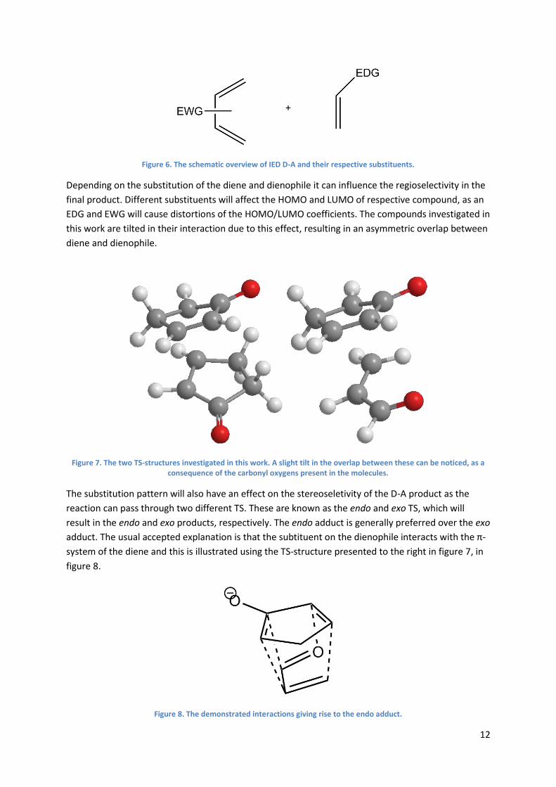
Figure 6. The schematic overview of IED D-A and their respective substituents.

Depending on the substitution of the diene and dienophile it can influence the regioselectivity in the

final product. Different substituents will affect the HOMO and LUMO of respective compound, as an

EDG and EWG will cause distortions of the HOMO/LUMO coefficients. The compounds investigated in

this work are tilted in their interaction due to this effect, resulting in an asymmetric overlap between

diene and dienophile.

Figure 7. The two TS-structures investigated in this work. A slight tilt in the overlap between these can be noticed, as a consequence of the carbonyl oxygens present in the molecules.

The substitution pattern will also have an effect on the stereoseletivity of the D-A product as the

reaction can pass through two different TS. These are known as the endo and exo TS, which will

result in the endo and exo products, respectively. The endo adduct is generally preferred over the exo

adduct. The usual accepted explanation is that the subtituent on the dienophile interacts with the π-

system of the diene and this is illustrated using the TS-structure presented to the right in figure 7, in

figure 8.

Figure 8. The demonstrated interactions giving rise to the endo adduct.

13

1.4 Mechanism of D-A with KSI After some review regarding KSI and its general function, now is the time to delve deeper into the

active mechanism of KSI and conveys the reason as to why this particular enzyme was chosen as a

candidate for Diels-Alderase. As previously mentioned, KSI is complexed with the steroid equilenin,

and even though the reaction mechanism for the isomerization of equilenin also has been pointed

out, it is worth going through it with accurate figures and explanation as this may serve an intuitive

purpose.

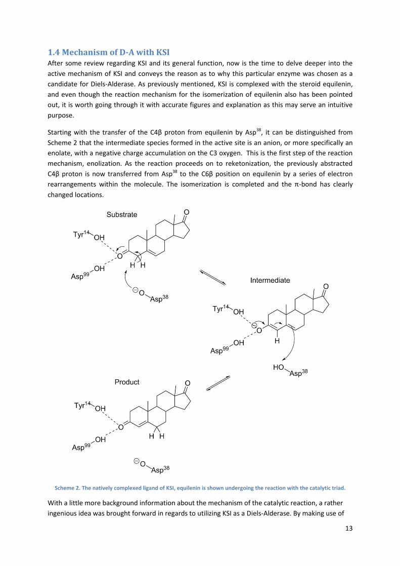
Starting with the transfer of the C4β proton from equilenin by Asp38, it can be distinguished from

Scheme 2 that the intermediate species formed in the active site is an anion, or more specifically an

enolate, with a negative charge accumulation on the C3 oxygen. This is the first step of the reaction

mechanism, enolization. As the reaction proceeds on to reketonization, the previously abstracted

C4β proton is now transferred from Asp38 to the C6β position on equilenin by a series of electron

rearrangements within the molecule. The isomerization is completed and the π-bond has clearly

changed locations.

Scheme 2. The natively complexed ligand of KSI, equilenin is shown undergoing the reaction with the catalytic triad.

With a little more background information about the mechanism of the catalytic reaction, a rather

ingenious idea was brought forward in regards to utilizing KSI as a Diels-Alderase. By making use of

14

an α,β-saturated ketone and the general acid/base mechanism in KSI, the abstraction of the ketones

α proton would generate a diene in situ, while the TS intermediate will attain stability through

interactions Asp99 and Tyr14. Earlier studies have shown that Asp38 is an accomplished base in

heterolytic cleavage of C-H bonds, which leaves for a broad possibility of substrate choices in regards

to pKa of the α-proton [7]. Although a diene can readily be generated within the active site of KSI

there is still the problem with the required s-cis conformation of the diene. A quite simple solution to

this problem would be to use cyclic α,β-saturated ketones as pro-dienes, seeing as the abstraction of

the α proton would result in an enolate species and thereby provide a diene in the correct s-cis

conformation.

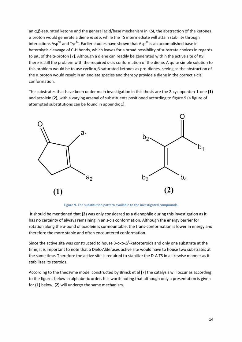
The substrates that have been under main investigation in this thesis are the 2-cyclopenten-1-one (1)

and acrolein (2), with a varying arsenal of substituents positioned according to figure 9 (a figure of

attempted substitutions can be found in appendix 1).

Figure 9. The substitution pattern available to the investigated compounds.

It should be mentioned that (2) was only considered as a dienophile during this investigation as it

has no certainty of always remaining in an s-cis conformation. Although the energy barrier for

rotation along the σ-bond of acrolein is surmountable, the trans-conformation is lower in energy and

therefore the more stable and often encountered conformation.

Since the active site was constructed to house 3-oxo-∆5-ketosteroids and only one substrate at the

time, it is important to note that a Diels-Alderases active site would have to house two substrates at

the same time. Therefore the active site is required to stabilize the D-A TS in a likewise manner as it

stabilizes its steroids.

According to the theozyme model constructed by Brinck et al [7] the catalysis will occur as according

to the figures below in alphabetic order. It is worth noting that although only a presentation is given

for (1) below, (2) will undergo the same mechanism.

15

Figure 10. The pro-diene is seen interacting with the Asp99

and Tyr14

in a) where the α-proton is about to be abstracted by Asp

38, generating the diene in situ. In b) the proton has successfully been abstracted and can be observed on Asp

38.

Figure 11. In c) the dienophile (another molecule of (2) here) has approached the diene from below and formed the first TS. d) Presents the anionic product obtained as the reaction has been performed.

Figure 12. The re-protonation with the proton still present on Asp38

in e) which is seen returned to its original position in f). The resulting product is the endo adduct of the two interacting molecules.

16

In their work, (1) was used as a substrate with the intention to act as both diene and dienophile.

Initially, the first molecule of (1) will form hydrogen bonds to Asp99 and Tyr14 with its ketone oxygen

acting as hydrogen bond acceptor, while simultaneously positioning its α proton in close proximity of

the basic Asp38 residue. Of course there will be no guarantee for a perfect adaption of orientation

immediately as the pro-diene approaches the active site, but a reaction will only occur as the α

proton is facing Asp38. In a swift fashion the second molecule of (1), the dienophile, will approach the

diene from ‘slightly beneath’, according to figure

Following the formation of the diene a regular D-A reaction would take place and a newly formed

product is obtained. From figure 12.f) it is worth noting the transfer of the proton to its original

position. The Endo adduct is also the most probable product to end up with in accordance with the

Endo rule described earlier (section 1.3).

2. Theoretical Overview

2.1. Molecular Docking Since the methodology known as molecular docking was established in the 1980:s [15] it has grown

to be a valuable asset in drug discovery, providing a fast and effective means of detecting potential

ligands to be used in drug design [16]. The field of molecular docking has led to a spread of different

computational docking programs which aims to perform a specific screening process, both

concerning protein-protein docking and protein-ligand docking, where a few assorted programs are

described elsewhere [17]. The remainder of this section will consider protein-ligand docking with the

AutoDock software as well as some brief review of the relevant background and coverage of some

off the more important parameter files in AutoDock [18].

2.1.1 Problems with Molecular Docking

The study of molecular interactions can reveal a tremendous amount of information regarding

biological processes. What makes molecular docking a complicated matter is the fact that enzymes

are dynamic entities, where the backbone possesses certain degrees of freedom and the side chains

can adapt different conformations. Of course, the ligand can explore some conformational space, but

the enzyme is a bit more restricted due to entropic penalties, causing some dynamic restrictions,

associated with enzyme movement [19].

In the common biochemistry class it is not unusual to introduce students to the well-known “lock and

key” description of a molecular interaction between enzyme and ligand. However, this analogy does

not describe the entire situation, mainly due to the fact that there is still a lot we do not know about

enzymes. Another good description that has been used is the “induced fit”, and this is considerably

closer to reality than the “lock and key” description [19]. Another good way of looking at the

situations is considering the system as a “hand in a glove” situation, where the glove is adapting

(within limits) to the different conformations the hand can adopt [17][20]. But the central purpose of

molecular docking is to, as earlier mentioned, efficiently screen a large set (or library) of compounds

against a macromolecular target with satisfactory precision. This means that the ligand should be

able to explore an extensive conformational space and ligand orientations with accurate

determination of binding mode and affinity towards the target, while still remaining computationally

fast [17][18]. By introducing flexible side chains in an enzyme there is a possibility of increasing the

17

prediction of correct binding modes at the cost of the simulation being more computationally

expensive, while at the same time increasing the chance of false positives amongst the result due to

the larger conformational space [42]. Since only a few side chain residues are considered as flexible,

this aspect fails to treat backbone mobility of the enzyme [20].

Although molecular docking is a quite difficult problem in regards to optimization, it is still an

extensively useful method in quickly predicting binding modes and affinities, as well as acquiring

starting coordinates for further analysis with for example molecular dynamics. Molecular dynamics

(treated explicitly later) aims to thoroughly analyze a ligands conformational space while treating the

entire enzyme as being dynamic, including backbone flexibility along with the different

conformations of the side chains. However, as this approach requires additional computational

power, molecular dynamics is not recommended for screening of compounds to the same extent as

docking. But how does the evaluation of binding affinity and binding modes occur in AutoDock?

2.1.2 AutoDock – A semi-empirical force field

AutoDock 4.2 utilizes a conceptually simple semi-empirical force field to evaluate the free binding

energy in the formation of a ligand-protein complex that has been parameterized by using a training

set consisting of a large number of protein-inhibitor complexes, where all 3D structures and inhibitor

constants KI had previously been determined. The information relayed in this section is based on the

work by Huey et al [21]. The force field utilizes a set of pair-wise evaluations V and the term ∆Sconf

describing the conformational entropy, which is lost upon the binding of the ligand to the

macromolecular target,

∆𝐺 = (𝑉𝑏𝑜𝑢𝑛𝑑𝐿−𝐿 − 𝑉𝑢𝑛𝑏𝑜𝑢𝑛𝑑

𝐿−𝐿 ) + (𝑉𝑏𝑜𝑢𝑛𝑑𝑃−𝑃 − 𝑉𝑢𝑛𝑏𝑜𝑢𝑛𝑑

𝑃−𝑃 ) + (𝑉𝑏𝑜𝑢𝑛𝑑𝑃−𝐿 − 𝑉𝑢𝑛𝑏𝑜𝑢𝑛𝑑

𝑃−𝐿 + ∆𝑆𝑐𝑜𝑛𝑓) Eq.1

Where L and P refers to the ligand and protein (or macromolecule) respectively. For each docking

simulation the binding energy is estimated in a two-step process where the first course of action is i)

to determine the energy that arises intramolecularly as both molecules transition from unbound to

bound conformation, where the two terms in the first parenthesis of Eq.1 describes the ligands

intramolecular energy in the bound and unbound states. The two terms in the second parenthesis

describes the same type of intramolecular interactions for the macromolecule. ii) The second

estimation occurs in the last parenthesis where the ligand forms a complex with the macromolecule,

and the intermolecular energy is evaluated. It is important to note that 𝑉𝑢𝑛𝑏𝑜𝑢𝑛𝑑𝑃−𝐿 will be zero, as it is

assumed that the ligand and protein are at a great enough distance from each other that no

interactions will take place.

Each pair-wise evaluation in eq.1 consists of terms that aim to describe enthalpic as well as entropic

contributions to the free binding energy and is described as follows:

𝑉 = 𝑊𝑣𝑑𝑤∑(𝐴𝑖𝑗

𝑟𝑖𝑗12 −

𝐵𝑖𝑗

𝑟𝑖𝑗6 ) +𝑊ℎ𝑏𝑜𝑛𝑑∑𝐸(𝑡) (

𝐶𝑖𝑗

𝑟𝑖𝑗12 −

𝐷𝑖𝑗

𝑟𝑖𝑗10) +

𝑖,𝑗

𝑊𝑒𝑙𝑒𝑐∑𝑞𝑖𝑞𝑗

휀(𝑟𝑖𝑗)𝑟𝑖𝑗+𝑊𝑠𝑜𝑙∑(𝑆𝑖𝑉𝑗 + 𝑆𝑗𝑉𝑖)𝑒

(−𝑟𝑖𝑗2

2𝜎2)

𝑖,𝑗𝑖,𝑗𝑖,𝑗

Eq.2

Where the interactions considered are dispersion/respulsion, hydrogen bonding, electrostatics and

desolvation, respectively.

Each respective interaction parameter is preceded by the experimentally determined weighting

factors W. The A and B are parameters retrieved from the AMBER force field [22]. E(t) is defined as a

18

weighted directional, where t is the angle away from ideal bonding geometry. The parameters C and

D have been assigned to have a maximum well depth for hydrogen bonds, where the depth is 5

kcal/mol for O-H, N-H at 1.9 Å and 1 kcal/mol for S-H at 2.5 Å. The third term is the electrostatic

interactions evaluated by a screened Coulomb potential. The fourth and last term contains the

desolvation potential which is dependent on the volume of atoms V surrounding particular atom,

shielding that atom from solvent molecules. S is the solvation parameter and σ is a distance-

weighted factor set to 3.5 Å. The conformational entropy that is lost upon binding of the ligand,

∆Sconf, is proportional to the amount of bonds with ability to rotate, Ntors, where all torsional degrees

of freedom are included and is described accordingly

∆𝑆𝑐𝑜𝑛𝑓 = 𝑊𝑐𝑜𝑛𝑓𝑁𝑡𝑜𝑟𝑠 Eq.3

2.1.3 Autogrid

To attain a swift performance when executing a docking simulation, AutoDock 4.2 makes use of pre-

calculated grid maps that contain information about interaction energies for a set of atom types

present in the ligand that is to be docked. These grid maps are calculated with the program AutoGrid.

In the ADT GUI, the dimensions of a grid box can be defined over a selected partition of the

macromolecule and by specifying the grid point spacing, each of these points houses information on

the potential energy of the atoms in the ligand in relation to the macromolecule.

AutoGrid requires a grid parameter file (.gpf) that among other things holds the information on what

maps should be generated for significant atom types, the size of the grid box along with coordinates

declaring its location, the rigid receptor to be used in the docking simulation and more.

It is important to remember that this is simply a pre-calculation to improve calculation speed. The

AutoGrid program manages to reduce the complexity of the problem from N2 to N, where N is the

number of interacting atoms [18][21].

2.1.4 Lamarckian Genetic Algorithm

The French scientist Jean-Baptiste de Lamarck took an interest in evolution during the late 1700s and

proposed an evolutionary theory that could be summed up as, whatever traits an individual acquires

during its lifetime will affect the individuals traits that it passes on to its offspring. Even though this is

generally agreed upon to be an incorrect understanding of how evolution works, Lamarck is

accredited as being the first to present a truly coherent evolutionary theory [23].

During a molecular docking simulation all orientational, conformational and positional samplings

needs to be explored, turning docking into a difficult optimization problem [18]. Genetic algorithms

(GA) have previously been successfully employed for these types of problems as they are effective in

conducting a global search. A GA intends to discover solutions by means of procedures that are

inspired by evolutionary principles. During a docking, a ligand is situated in a particular state in

relation to the protein, where the translation, orientation and conformation of said ligand is

described by a set of values. If these values changes, the same is true for the ligands state. This is

therefore known as a ligands state variables and in a GA each state variable constitutes a particular

gene. This means that the entire ensemble of state variables makes up the ligands, or individuals,

genotype. The individual’s genotype is mapped by applying a developmental mapping function to its

corresponding phenotype, which composes the ligands atomic coordinates. As the phenotype has

been mapped the individual’s fitness is evaluated, where the fitness corresponds to the total energy

19

of interaction between a ligand and a protein. Similarly, this methodology is applied for the entirety

of the population.

The user is free to choose between a GA, an adaptive Local Search method (LS) or a hybrid GA-LS

method in AutoDock 4.2. The LS performs local energy minimizations and depending on the

previously registered energies, the step size is adjusted, where an increase in energy will double the

step size and a decrease in energy will result in the step size being halved. The adaptive LS is based

on work by Solis and Wets [24]. The combination of the GA and adaptive LS is what composes the

LGA. But the aspect of what makes this hybrid method “Lamarckian” has yet to be mentioned.

As the global search is performed, occasionally, a random mutation will arise, which might improve

the fitness of a certain individual. During the mating between two individuals it is possible that there

will be a crossover of genetic material that is passed on to the offspring, where the offspring can

plausibly be evaluated as being better fit than its parents. This is all in accordance with Darwinian

and Mendelian genetics [18]. As the LS progresses the phenotype can readily be altered, meaning

that the ligand performs some local movement, resulting in an energy decrease (increased fitness).

From the current phenotype there can be an inverse mapping to the genotype. This is analogue to

Lamarck’s claims about traits that are acquired during an individual’s lifetime can be effectively

transmitted to its offspring. The inverse mapping from the phenotype to the genotype is therefore by

definition “Lamarckian”, ultimately resulting in the LGA.

2.2 Molecular Dynamics There are several different biological systems that are seemingly interesting to study and that have

been studied on a macroscopic level. These systems commonly contain an overwhelming number of

particles and therefore also present a large number of conformations and unique interactions that

appear insurmountable in regards of detailed inspection. An investigation can however be performed

through the use of computer-aided simulations, where a small portion of these macroscopic systems

can be properly examined, but with a considerably less amount of particles included. Different

approaches have been taken to achieve manageable systems that can be carefully studied, where

one of the most famous methods employed is the Monte Carlo method. The general concept of the

Monte-Carlo method is to gather a lot of samplings by randomly generating a certain trial move and

then making a choice of whether to accept or reject the move. Although the Monte Carlo method

has proved useful in its application of randomness in studying for example fluid dynamics, it does not

consider changes over time. When contemplating various biological systems such as substrate

passage between transmembrane proteins, determination of binding free energies between ligand-

enzyme complexes and protein folding analysis (only to name a few), including time-dependency

serves to quite accurately describe the step-wise development of the system that one seeks to study.

At the same time, in order to obtain the sought after accuracy of these time-dependent biological

systems the employment of molecular dynamics (MD) are of utmost necessity. Additionally, in order

to describe these macroscopic systems at a suitable microscopic level, namely through expression of

atomic positions and their respective velocities, statistical mechanics are of essence. Since MD

simulations treat clearly large N-body problems, a means of rationalizing these computationally

demanding calculations is via utilization of mechanical force fields.

Following this introductory passage will be a brief overview of statistical mechanics, the fundamental

aspects of a typical MD simulation while also including some parts on force fields.

20

All theory in this section is taken from Molecular Modelling – Principles and Applications by Andrew

Leach [25].

2.2.1 Statistical Mechanics

The association between simulations at the microscopic level and macroscopic properties is made

with the help of statistical mechanics. The very purpose of statistical mechanics is to find a way to

study macroscopic properties through the use of the microscopic simulations, or more accurately

put, to describe macroscopic properties with the help of position and momentum for each of the N

particles present in the system. A useful approach in defining the state of the system comprised of N

particles is that the position can be described by 3N coordinates and the momenta can be described

by 3N components, resulting in 6N dimensions which define the system. More accurately, the

position and momenta of these particles are what define a microscopic state and the 6N dimension

made up from these particles is referred to as the phase space. As a single point in phase space

assists in the description of a systems current state, an entire collection of these single points makes

up what is known as an ensemble, and an ensemble is a collection of microscopic states. These

ensembles are used as expectation values in statistical mechanics, implying that a macroscopic

system could be viewed upon as a series of replications which are all considered at the same time.

This situation can be described by the following expression

⟨𝐴⟩𝑒𝑛𝑠 = ∫∫𝑑𝒑𝑁 𝑑𝒓𝑁𝐴(𝒑𝑁 , 𝒓𝑁) 𝜌(𝒑𝑁 , 𝒓𝑁) Eq.4

Where ⟨𝐴⟩ is the ensemble average, or the average value of the property A taken over all replications

of the system and

𝐴(𝒑𝑁 , 𝒓𝑁) Eq.5

Describes the property A as a function of the momenta p and position r in the system. Also, the

𝜌(𝒑𝑁 , 𝒓𝑁) Eq.6

Is the ensembles probability density, given by

𝜌(𝒑𝑁 , 𝒓𝑁) =1

𝑄exp(−

𝐸(𝒑𝑁 , 𝒓𝑁)

𝑘𝐵𝑇)

Eq.7

Where E is the energy, T is temperature and 𝑘𝐵 is the Boltzmann constant. Q is the partition function

and can be written as

𝑄 =∫∫𝑑𝒑𝑁 𝑑𝒓𝑁 exp(−Ĥ(𝒑𝑁, 𝒓𝑁)

𝑘𝐵𝑇)

Eq.8

Since this describes the overall procedure to estimate the properties of a macroscopic system by the

evaluation of the ensemble average of A, how does the approach look for a MD simulation where

time-dependency is introduced? Well, it is in fact very similar, except it has to be considered that a

21

macroscopic system usually contains numbers of atoms in the order of 1023 and solving this while

including time-dependency is unfeasible with modern computational power. The integral presented

in Eq.4 is complex in itself, implying that a different route has to be taken to establish a time-

dependent MD simulation with an acceptable computational time. For a system comprised of N

number of particles, the instantaneous value of the property A may be expressed as

𝐴(𝒑𝑁(𝑡), 𝒓𝑁(𝑡)) ≡ 𝐴(𝑝1𝑥, 𝑝1𝑦, 𝑝1𝑧, 𝑝2𝑥 , … , 𝑥1, 𝑦1, 𝑧1, 𝑥2, … , 𝑡) Eq.9

Where 𝑝1𝑥refers to the momentum of particle 1 in the x direction where 𝑥1 is the momentums x

coordinate and so on. As the instantaneous value is reliant on the changes occurring over time in the

system due to different interactions between particles taking place, it is appropriate to express the

property A as an average value even in the MD simulation. This average is based on the simulation

time, resulting in the time average of the property A, expressed by

⟨𝐴⟩𝑡𝑖𝑚𝑒 = lim𝜏→∞

1

𝜏∫ 𝐴(𝒑𝑁(𝑡), 𝒓𝑁(𝑡))𝑑𝑡

𝜏

𝑡=0

≈1

𝑀∑𝐴(𝒑𝑁, 𝒓𝑁)

𝑀

𝑡=1

Eq.10

Where t is the simulation time and M is the number of time steps exercised during simulation and

𝐴(𝒑𝑁 , 𝒓𝑁) is the instantaneous value of property A.

Hence, both microscopic and macroscopic properties can be described with statistical mechanics. But

a key component is still lacking as MD simulations averages over time and experimental performance

samples ensemble averages. By employing the ergodic hypothesis the microscopic and macroscopic

systems can be evaluated on the following assumption

⟨𝐴⟩𝑒𝑛𝑠 = ⟨𝐴⟩𝑡𝑖𝑚𝑒 Eq.11

The ergodic hypothesis states that a system may explore each and every possible state if it is allowed

to continue indefinitely through time. As such it is impeccable that a MD simulation manages to

sample enough of the phase space as a fixed time limit is specified for a simulation run. If enough

states are explored one can claim that the MD simulation will correspond to experimental accuracy.

There are ways to effectively perform MD simulations with fewer particles without penalizing the

‘real’ behavior of the system. The use of periodic boundary conditions (PBC) serves to limit the

number of particles; therefore successfully lowering the computation time as the number N will be

lower. A simulation may then be conducted for a satisfactory amount of time, producing a required

amount of conformations.

2.2.2 Molecular Dynamics simulation

The primary goal for an MD simulation is to evaluate the exerted force arising upon the interactions

of particles within a system. This information is thus obtained by solving the Newton’s equations of

motion,

𝑭 = 𝒎𝒂 Eq.12

This equation houses a differential equation as well which can be presented as

22

𝑑2𝒓𝑖𝑑𝑡2

=𝑭𝑖𝒎𝑖

Eq.13

Where 𝒓𝑖 is the position of the particle, 𝒎𝑖 its mass and 𝑭𝑖 the force applied on said particle in a

particular direction. To study the dynamics of the system, at a certain time t, the particles initial

position, its velocity and the acceleration should be known. These parameters have been

approximated with a Taylor series expansion while considering the position 𝒓(𝑡) and the time steps

before, 𝒓(𝑡 + 𝛿𝑡) and after, 𝒓(𝑡 − 𝛿𝑡). The Taylor expansions are presented accordingly

𝑖)𝒓(𝑡 + 𝛿𝑡) = 𝐫(t) + 𝐯(t)𝛿𝑡 +1

2𝒂(𝑡)𝛿𝑡2 +

1

6𝒃(𝑡)𝛿𝑡3 +⋯ Eq.14

𝑖𝑖)𝒓(𝑡 − 𝛿𝑡) = 𝐫(t) − 𝐯(t)𝛿𝑡 +1

2𝒂(𝑡)𝛿𝑡2 −

1

6𝒃(𝑡)𝛿𝑡3 +⋯ Eq.15

When i) and ii) are added it produces the following

𝒓(𝑡 + 𝛿𝑡) + 𝒓(𝑡 − 𝛿𝑡) = 2𝐫(t) + 𝒂(𝑡)𝛿𝑡2 + 𝑂(𝛿𝑡4) Eq.16

That can be rearranged to

𝒓(𝑡 + 𝛿𝑡) = 2𝐫(t) − 𝒓(𝑡 − 𝛿𝑡) + 𝒂(𝑡)𝛿𝑡2 Eq.17

Resulting in the original Verlet algorithm. From Eq.16 it can be seen that the Verlet algorithm will be

correct up to 4th order in positions. In the expression, 𝐫(t) represents the position and 𝒂(𝑡) is simply

the acceleration. The velocity 𝐯(t) is not explicitly included in the Verlet algorithm as the addition of

i) and ii) cancels the term out. One can however calculate the velocity from the information provided

by the positions

𝐯(t) =𝒓(𝑡 + 𝛿𝑡) − 𝒓(𝑡 − 𝛿𝑡)

2𝛿𝑡 Eq.18

Overall the calculation Verlet algorithm follows the following sequence:

1. Determine 𝒂(𝑡) from the force, 𝐹[𝒓(𝑡)}/𝑚.

2. Calculate 𝒓(𝑡 + 𝛿𝑡) from 𝒂(𝑡) and 𝒓(𝑡 − 𝛿𝑡).

3. If desired, 𝐯(t) can be determined as in Eq.18

Dynamic systems are reliant on choosing a fitting enough time step, which can be described as a

sequence of frames, similarly to when filming movies during the era of Buster Keaton. If a time step

is chosen and appears too small, the trajectory will only explore a narrow part of phase space. A too

large time step will cause the sought after event to be missed, as the simulation will produce a too

great of a separation, due to a cause of overestimated energy between particles.

2.2.3 Classical mechanics - Force fields

When studying biological systems one usually works with an amount of particles which cannot be

treated with methods from quantum chemistry, or even the most fitting of MD algorithms. As has

23

been discussed in the section of Statistical mechanics, MD simulations make use of the property A

and ultimately ensemble averages. Molecular mechanics are used in order to make calculations like

this feasible, where force fields are employed to describe the general interactions of atoms. A

potential energy surface (PES) is used to describe a molecule’s energy as a function of geometry and

a PES is helpful when parametrizing a force field.

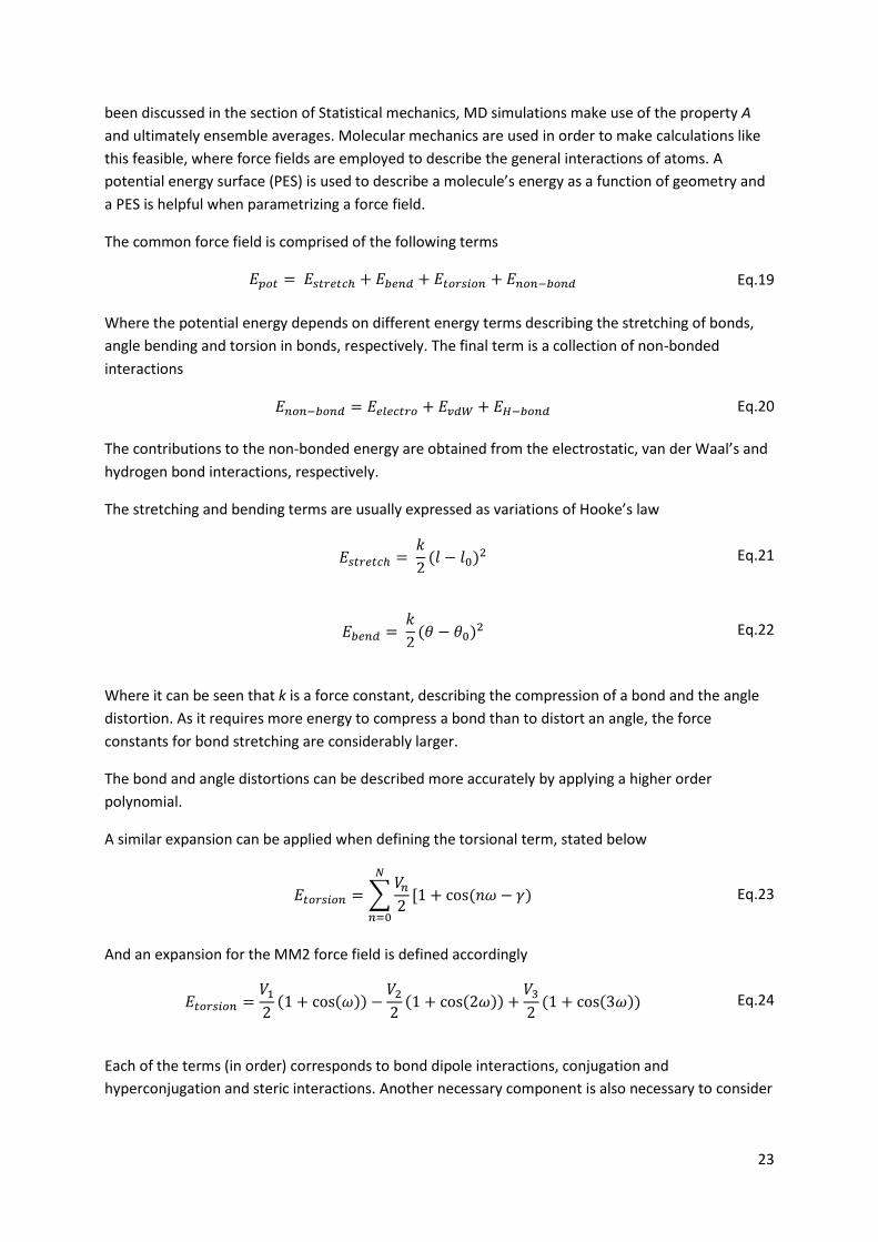
The common force field is comprised of the following terms

𝐸𝑝𝑜𝑡 =𝐸𝑠𝑡𝑟𝑒𝑡𝑐ℎ + 𝐸𝑏𝑒𝑛𝑑 + 𝐸𝑡𝑜𝑟𝑠𝑖𝑜𝑛 + 𝐸𝑛𝑜𝑛−𝑏𝑜𝑛𝑑 Eq.19

Where the potential energy depends on different energy terms describing the stretching of bonds,

angle bending and torsion in bonds, respectively. The final term is a collection of non-bonded

interactions

𝐸𝑛𝑜𝑛−𝑏𝑜𝑛𝑑 = 𝐸𝑒𝑙𝑒𝑐𝑡𝑟𝑜 + 𝐸𝑣𝑑𝑊 + 𝐸𝐻−𝑏𝑜𝑛𝑑 Eq.20

The contributions to the non-bonded energy are obtained from the electrostatic, van der Waal’s and

hydrogen bond interactions, respectively.

The stretching and bending terms are usually expressed as variations of Hooke’s law

𝐸𝑠𝑡𝑟𝑒𝑡𝑐ℎ =𝑘

2(𝑙 − 𝑙0)

2 Eq.21

𝐸𝑏𝑒𝑛𝑑 =𝑘

2(𝜃 − 𝜃0)

2 Eq.22

Where it can be seen that k is a force constant, describing the compression of a bond and the angle

distortion. As it requires more energy to compress a bond than to distort an angle, the force

constants for bond stretching are considerably larger.

The bond and angle distortions can be described more accurately by applying a higher order

polynomial.

A similar expansion can be applied when defining the torsional term, stated below

𝐸𝑡𝑜𝑟𝑠𝑖𝑜𝑛 = ∑𝑉𝑛2

𝑁

𝑛=0

[1 + cos(𝑛𝜔 − 𝛾) Eq.23

And an expansion for the MM2 force field is defined accordingly

𝐸𝑡𝑜𝑟𝑠𝑖𝑜𝑛 =𝑉12(1 + cos(𝜔)) −

𝑉22(1 + cos(2𝜔)) +

𝑉32(1 + cos(3𝜔)) Eq.24

Each of the terms (in order) corresponds to bond dipole interactions, conjugation and

hyperconjugation and steric interactions. Another necessary component is also necessary to consider

24

regarding angular terms, namely the part treating the out-of-plane bending along with improper

torsion. Three of the common methods employed are the angle-to-plane

𝜐(𝜃) =𝑘

2𝜃2 Eq.25

The distance-to-plane

𝜐(ℎ) =𝑘

2ℎ2 Eq.26

And the third component considers the improper torsion

𝜐(𝜔) = 𝑘(1 − cos(2𝜔)) Eq.27

It is time to consider the expressions used for the non-bonding part of common force fields.

Electrostatic interactions in MD simulations cannot be accounted for by molecular orbital (MO)

calculations for the simple reason that the system is too big. The calculations would be far too

expensive, which leaves for a different approach to estimate the charges. It is common to assign

Coulombic interactions to describe the electrostatics with a dielectric constant that averages the

polarization effects

𝐸𝑒𝑙𝑒𝑐𝑡𝑟𝑜 =∑∑𝑞𝑖𝑞𝑗

4𝜋휀0𝑟𝑖𝑗

𝑁𝐵

𝑗=1

𝑁𝐴

𝑖=1

Eq.28

Where NA and NB are the number of point charges for two molecules,휀0 is the dielectric constant and

𝑟𝑖𝑗 is the distance between to charges.

The last two non-bonding terms employ different potentials. The van der Waal interactions use a

6/12 potential, more commonly known as the Lennard-Jones potential

𝐸𝑣𝑑𝑊 = 4휀𝑖𝑗 [(𝜎𝑖𝑗

𝑟𝑖𝑗)

12

− (𝜎𝑖𝑗

𝑟𝑖𝑗)

6

] Eq.29

The potential for hydrogen bonds is not always included but holds a similar appearance to the L-J

potential. However, it is necessary to know the identities of the hydrogen bonds before the

calculation is performed.

All parameters has now been the subject of a brief overview and the MD section closes with the full

expression for a basic MM force field

𝐸𝑝𝑜𝑡(𝒓𝑁) = ∑

𝑘𝑖2(𝑙𝑖 − 𝑙0,𝑖)

2

𝑏𝑜𝑛𝑑𝑠

+ ∑𝑘𝑖2(𝜃𝑖 − 𝜃0,𝑖)

2

𝑎𝑛𝑔𝑙𝑒𝑠

+ ∑𝑉𝑛2

𝑡𝑜𝑟𝑠𝑖𝑜𝑛𝑠

(1 + cos(𝑛𝜔 − 𝛾))

+∑ ∑ (4휀𝑖𝑗 [(𝜎𝑖𝑗

𝑟𝑖𝑗)

12

− (𝜎𝑖𝑗

𝑟𝑖𝑗)

6

] +𝑞𝑖𝑞𝑗

4𝜋휀0𝑟𝑖𝑗)

𝑁

𝑗=𝑖+1

𝑁

𝑖=1

Eq.30

25

2.3 Quantum Chemistry Quantum mechanics (QM) is agreed to be one of the most profoundly shocking theories to ever have

been established and despite being a particularly difficult subject, it has evolved rapidly during the

past hundred years while revolutionizing both scientific conduct and society. A long time has passed

since the early 1900s and QM has evolved into a pragmatic tool, not least within chemistry.

Computational chemists rely on Quantum chemical (QC) principles to investigate molecular systems,

reaction mechanisms, activation barriers etc. However, the equations describing these systems are

quite complex and striving for exact solutions with modern QC methods are simply not possible. The

sophisticated nature of molecular systems is notably obvious when evaluated by a QC approach and

one quickly finds that as the number of particles increases, so does the computational time and

power as well, sometimes drastically. Hence computational chemists are relying on good

approximations that can be made to simplify necessary calculations while maintaining satisfactory

enough solutions. Coincidentally, enhanced computational power share an equal amount of benefits

as good approximations, if not more.

This section aims to give a brief review of the fundamental aspects of QC and shortly mention some

of the methods, while finishing with an overview of the method used in this thesis, Density

Functional Theory (DFT).

All theory regarding the QC principles are taken from the text book Modern Quantum Chemistry:

Introduction to Advanced Electronic Structure Theory, by Szabo and Ostlund [26].

2.3.1 The Schrödinger equation

It is not an overstatement in that Edwin Schrödinger, by publishing his work on the widely known

partial differential equation bearing his own name, revolutionized physics [27].

Ĥ𝛹 = 𝐸𝛹 Eq.31 Where Ĥ is the Hamiltonian, Ψ is the wave function of the system and E is the energy obtained as an

eigenvalue to the Hamiltonian operator. The Hamiltonian operator is therefore a descriptor of the

systems total energy and is comprised of the quantum mechanical operators for kinetic and potential

energy. This includes terms that treats kinetic and potential energy for both nuclei and electrons and

as the particles number increases, so does the computational demands for that system.

The Hamiltonian is defined for N electrons and M nuclei as

Ĥ = −∑1

2∇𝑖2 −∑

1

2𝑀𝐴∇𝐴2 −∑∑

𝑍𝐴𝑟𝑖𝐴

+∑∑1

𝑟𝑖𝑗+∑ ∑

𝑍𝐴𝑍𝐵𝑅𝐴𝐵

𝑀

𝐵>𝐴

𝑀

𝐴=1

𝑁

𝑗>𝑖

𝑁

𝑖=1

𝑀

𝐴=1

𝑁

𝑖=1

𝑀

𝐴=1

𝑁

𝑖=1

Eq.32

Where MA is the ratio of the masses of nucleus A to an electron and ZA is nucleus A: s atomic number.

The operators ∇𝑖2 and ∇𝐴

2 are of Laplacian nature and handles differentiation regarding the

coordinates of the ith electron and the Ath nucleus. The terms in Eq. 32 corresponds to the kinetic

energy for electrons, kinetic energy for nuclei, coulombic interactions between the electrons and

nuclei, electron repulsion and nuclei repulsion respectively.

As a solution to the Schrödinger equation is sought after, the Hamiltonian should bring about some

cause for concern for a computational chemist, as the operator contains several terms to be

evaluated. Given that the system also consists of a lot of particles this calls for extensive

26

computational demand. It is still possible to withhold exact solutions of the wave function, assuming

the system is off an extremely simple nature, although most investigations will not be conducted on

simple systems. How can the computational demands be met for complicated systems while still

producing accurate enough results which reflect reality?

2.3.2 The Born-Oppenheimer approximation

The applied solution to this problem is known as the Born-Oppenheimer approximation and it makes

use of the fact that atomic nuclei are heavier by a considerable amount when compared to the

electron. As the nuclei have greater mass than electrons it is naturally assumed that electrons

outmaneuver nuclei fairly easily, in regards of speed. A fitting approximation is therefore that the

nuclei of a molecule can be considered as fixed and that the electrons move in a field relative to the

fixed nuclei. With all taken in consideration, the Hamiltonian can now be written as

Ĥ𝑒𝑙𝑒𝑐𝑡𝑟𝑜𝑛 = −∑1

2∇𝑖2 −

𝑁

𝑖=1

∑∑𝑍𝐴𝑟𝑖𝐴

+∑∑1

𝑟𝑖𝑗

𝑁

𝑗>𝑖

𝑁

𝑖=1

𝑀

𝐴=1

𝑁

𝑖=1

Eq.33

Since the nuclei are regarded as fixed the term associated with the nuclei kinetic energy can be

neglected. The nuclei repulsion can be treated as constant and is added to the operator eigenvalue.

The resulting Hamiltonian is known as the electronic Hamiltonian and this indicates that the

Schrödinger equation could be solved simply by regarding the motions of N electrons in the field of

M point charges. This abbreviates the Schrödinger equation into the following format

Ĥ𝑒𝑙𝑒𝑐𝑡𝑟𝑜𝑛𝛹𝑒𝑙𝑒𝑐𝑡𝑟𝑜𝑛 = 𝐸𝑒𝑙𝑒𝑐𝑡𝑟𝑜𝑛𝛹𝑒𝑙𝑒𝑐𝑡𝑟𝑜𝑛 Eq.34

The assumption resulting in the electronic Schrödinger constitutes a major simplification compared

to the many-particle Schrödinger equation. However, although the electronic Schrödinger results in a

drastic decrease of computational effort, the fact remains that producing a solution still requires

solving a problem consisting of multiple components. Still, this approximation is more than enough

and is a vital part in the field of quantum chemistry.

2.3.3 Methods for solving the electronic Schrödinger equation

One of the most widely recognized approaches in attempting to solve the electronic Schrödinger was

presented in 1930 by Hartree and Fock, and is attributed as the Hartree-Fock approximation.

According to the HF approximation a wave function can be expressed as a Slater determinant. The

relevant background will be quickly summarized below.

In the beginning of the era of quantum mechanics the concept of electron spin was established,

where functions describing if an electron possessed the property of spin up, alternatively spin down,

was presented. By incorporating a so called spin coordinate, electrons could be defined by 3 spatial

coordinates alongside the spin property, allowing for the possibility of two spin orbitals. Each spin

orbital follows the Pauli principle, meaning that each spin orbital can house a maximum of one

electron. The electrons should also be indistinguishable in which orbital houses them. Because of this

the interchange of electrons can follow a symmetrical or anti-symmetrical approach. If the criterion

of indistinguishable electrons is met, a wave function can be formulated, consisting of a linear

combination of two wave functions. The two respective wave functions contain information about

the electron spin, and these wave functions can be expressed as the Slater determinant, where the

27

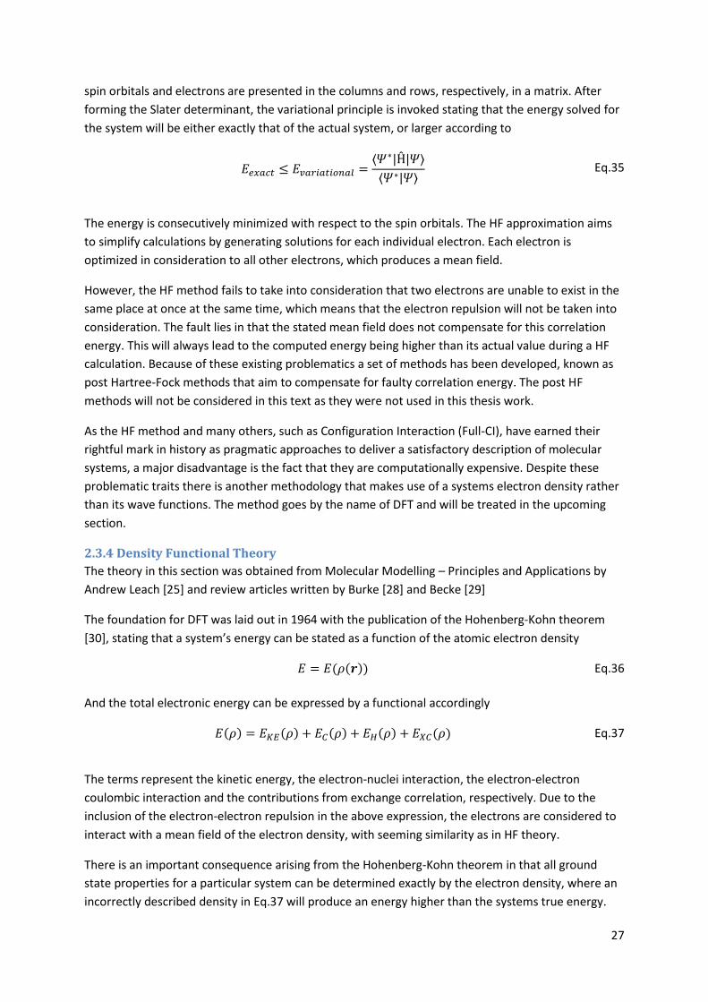
spin orbitals and electrons are presented in the columns and rows, respectively, in a matrix. After

forming the Slater determinant, the variational principle is invoked stating that the energy solved for

the system will be either exactly that of the actual system, or larger according to

𝐸𝑒𝑥𝑎𝑐𝑡 ≤ 𝐸𝑣𝑎𝑟𝑖𝑎𝑡𝑖𝑜𝑛𝑎𝑙 =⟨𝛹∗|Ĥ|𝛹⟩

⟨𝛹∗|𝛹⟩ Eq.35

The energy is consecutively minimized with respect to the spin orbitals. The HF approximation aims

to simplify calculations by generating solutions for each individual electron. Each electron is

optimized in consideration to all other electrons, which produces a mean field.

However, the HF method fails to take into consideration that two electrons are unable to exist in the

same place at once at the same time, which means that the electron repulsion will not be taken into

consideration. The fault lies in that the stated mean field does not compensate for this correlation

energy. This will always lead to the computed energy being higher than its actual value during a HF

calculation. Because of these existing problematics a set of methods has been developed, known as

post Hartree-Fock methods that aim to compensate for faulty correlation energy. The post HF

methods will not be considered in this text as they were not used in this thesis work.

As the HF method and many others, such as Configuration Interaction (Full-CI), have earned their

rightful mark in history as pragmatic approaches to deliver a satisfactory description of molecular

systems, a major disadvantage is the fact that they are computationally expensive. Despite these

problematic traits there is another methodology that makes use of a systems electron density rather

than its wave functions. The method goes by the name of DFT and will be treated in the upcoming

section.

2.3.4 Density Functional Theory

The theory in this section was obtained from Molecular Modelling – Principles and Applications by

Andrew Leach [25] and review articles written by Burke [28] and Becke [29]

The foundation for DFT was laid out in 1964 with the publication of the Hohenberg-Kohn theorem

[30], stating that a system’s energy can be stated as a function of the atomic electron density

𝐸 = 𝐸(𝜌(𝒓)) Eq.36

And the total electronic energy can be expressed by a functional accordingly

𝐸(𝜌) = 𝐸𝐾𝐸(𝜌) + 𝐸𝐶(𝜌) + 𝐸𝐻(𝜌) + 𝐸𝑋𝐶(𝜌) Eq.37

The terms represent the kinetic energy, the electron-nuclei interaction, the electron-electron

coulombic interaction and the contributions from exchange correlation, respectively. Due to the

inclusion of the electron-electron repulsion in the above expression, the electrons are considered to

interact with a mean field of the electron density, with seeming similarity as in HF theory.

There is an important consequence arising from the Hohenberg-Kohn theorem in that all ground

state properties for a particular system can be determined exactly by the electron density, where an

incorrectly described density in Eq.37 will produce an energy higher than the systems true energy.

28

Should the density be exactly described, one would also know external potential (namely, the

electron-nuclei interaction) and therefore the unique wave function for that system, indicating that

in theory everything is known. But this knowledge is not enough and a DFT variational principle is

required to, as accurately as possible, describe the system. For DFT, this means that the lowest

energy determined will conform to the systems exact density.

In the most common formulation of DFT, presented by Kohn and Sham, the approach taken is that a

single Slater determinant, comprised of orthonormal and real molecular orbitals, will represent the

density. This will result in the so called ‘Kohn-Sham orbitals’, which aim to optimize the systems

energy by solving a set of one-electron equations. However, since DFT takes the mean field approach

it is also necessary to include the electronic correlation. With respect to the aforementioned criteria

the Kohn-Sham equations are presented

[−∇2

2+ 𝑉𝑛𝑢𝑐𝑙𝑒𝑎𝑟(𝒓) + ∫𝑑𝑣´

𝜌(𝒓)

|𝒓 − 𝒓´|+ 𝑉𝑋𝐶(𝒓)]𝛹𝑖(𝒓) = 휀𝑖𝛹𝑖(𝒓) Eq.38

Where the exchange-correlation functional, 𝑉𝑋𝐶(𝒓), can be obtained from analytical expressions for

the local density approximation (LDA), which assumes that there exists a uniform electron gas model

that claims the electron density is constant in all space. Given the assumption that the charge density

through a molecule varies slowly (i.e, behaving as a uniform electron gas), if the exchange-correlation

energy per particle in the uniform gas is given by 휀𝑋𝐶 , then the total exchange-correlation energy,

𝐸𝑋𝐶 , as a consequence of being integrated over all space is given by

𝐸𝑋𝐶[𝜌(𝒓)] ≅ ∫𝜌(𝒓)휀𝑋𝐶 [𝜌(𝒓)]𝑑𝒓 Eq.39

The functional describing the exchange-correlation can then be written as

𝑉𝑋𝐶(𝒓) =𝛿𝐸𝑋𝐶[𝜌(𝒓)]

𝛿𝜌(𝒓) Eq.40

As the LDA incorporates the mean field approximation the exchange correlation energy is penalized

upon evaluation, approaches have been taken to compensate for this. An early example of attempts

to minimize the error was the incorporation of generalized gradient approximations (GGA: s), which

will not be examined further here [31]. The GGA: s showed improved accuracy upon application in

calculations of chemical nature and in the 1990s, the German native Axel D. Becke introduced hybrid

functionals [32], where perhaps the most famous functional used in modern DFT is the B3LYP

functional, where a mixture of GGA and HF exchange was introduced.

The peculiar thing about hybrid functionals is that they all have to be selected with care for what

particular system one intends to investigate. In this thesis, the B3LYP functional was not incorporated

as it has been noted previously that this functional do not perform adequately in describing the D-A

reaction [7]. Instead, the M06-2X functional by Truhlar [33] has been the preferred method of

execution, as inspired by the findings of Brinck et al [7].

29

3. Methodology

3.1 Computational details

3.1.1 Protein preparation

The enzyme crystal structure for Pseudomonas testosterone Kestosteroid Isomerase was retrieved

from the Protein Data Bank with the PDB entry 1QJG. The PDB structure was minimized using the

AMBER14 set of programs with the AMBER FF14SB force field and the side chain Asp38 was

protonated using the mutagenesis tool in PYMOL. To conduct the docking experiment, a pdbqt-file

for the rigid part and the flexible parts of the enzyme was prepared with AutoDock Tools. The

catalytic triad consisting of Tyr14, Asp38 and Asp99 were selected as flexible residues and separated

into an enzyme_flex.pdbqt file. The remaining side chains were incorporated in an

enzyme_rigid.pdbqt file. ADT was then used to set the grid box for the docking simulation, where the

box dimensions used initially was x = 40, y = 40, z = 40, and the grid box was defined around the

active site, making sure to include all important side chains. These settings were saved in a .gpf file.

3.1.2 Ligand preparation

Starting coordinates for the TS structures of acrolein and cyclopentenone were obtained from Brinck

et al (artikel IX – envisioning diels alderase). Utilizing this scaffold, substituents were added to the

different sites presented in Figure… with Gaussview. The coordinates for the TS structures was locked

in place and the substituents was geometrically optimized, along with a computation of the atomic

charges with DFT, using the M06-2X functional at the 6-31+G(d) level. The ligands was then

converted from .pdb to .pdbqt format using ADT, with the DFT-computed charges added to the

.pdbqt file. The raccoon program was used to prepare multiple ligands for docking simultaneously

(raccoon reference). Using the Raccoon GUI, all ligands were added together with the rigid and

flexible part of the enzyme. The .gpf file containing the information on the grid box was incorporated

as well, and the .dpf file was generated in Raccoon. Following this step, AutoGrid was run in order to

generate grid maps. The LGA was used to create up to 100 conformations at a time, with 2 500 000

energy evaluations and 40 000 as a maximum number of generations.

3.1.3 Molecular dynamics preparation

The MD simulations were performed with the AMBER14 [34] set of programs, using the Amber force

field: FF14SB [35]. The general Amber force field (GAFF) [36] was employed to obtain force field

parameters for the ligands by using Antechamber [37] and Parmchk [38] in AmberTools. The partial

charges for the ligands were computed using RESP charges [39]. The enzyme was charge neutralized

using 2 Cl- ions and solvated with TIP3P water [40] (8.0 Å solvent shell) using XLEaP. The systems

were minimized two times using Sander, where the first minimization ran for 1000 iterations while

holding the protein fixed and the second minimization ran for 2500 iterations with no constriction to

the protein. For the minimization a steepest descent algorithm was performed for the first half of

both simulations and the other half of the minimization employed a conjugate gradient method.

Following the minimization the systems were heated to 300 K for duration of 20 ps, while putting

mild restraints on the protein. Unconstrained production was then performed, using pmemd.CUDA

[41], for 4 ns with a temperature of 300 K, pressure at 1 bar and a 2 fs time step. For hydrogen

atoms, the SHAKE algorithm was used. Lastly, trajectory analysis was performed with the program

CPPTRAJ in AmberTools.

30

4. Results and Discussion

4.1 Molecular Docking with AutoDock 4.2

Figure 13. An example of a docked structure, presented more thorough later in the text.

Earlier work, performed by Brinck et al, determined that KSI had the potential to house a D-A

reaction as it contained relevant catalytic components to generate an in-situ diene by proton

abstraction [7]. Although the catalytic mechanism was investigated, an evaluation of beneficial

substrate and enzyme design was not covered by the investigation at the time. A presentation of the

investigation conducted during this thesis will be presented below, dealing with the different aspects

of advantageous design, both in regards to the evaluated substrates and the attempts at a better

suited active site.

4.1.1 Initial findings

Figure 14. An extracted sample of some residues making up the active site of KSI.

31

Initial screenings using (1) (Figure 7 and 9) as diene and dienophile did not provide satisfactory poses

and demonstrated weak binding affinities in the wildtype KSI (hits with binding affinities higher than

-5.0 kcal/mol were discarded). As the substrates based on this scaffold would not yield a sought after

result the decision was made to solely focus on the 2-cyclopenten-1-one/Acrolein TS scaffold.

However, initial dockings with the monosubstituted (1) did indicate that a pyridine-based substituent

in the b2 position of the dienophile (Figure 7) presented some poses where the interactions between

substrate and the catalytic triad were upheld, although the planar positioning required in respect to

Asp38 was absent. It could also be determined that the binding-affinity slightly increased for all

attempted disubstituted substrates where pyridine was utilized as a substituent on the dienophile,

while retaining some interactions necessary for catalysis, yet still not to a satisfactory extent. Due to

these findings alone it was decided to further the investigation with pyridine as a plausible

substituent fitting for the dienophile, while shifting focus to the (2) compound, which was considered

as the dienophile throughout the rest of this work.

After obtaining a plausible dienophile the screening continued with attempted substitutions at the

b1 position on the diene. The reasoning was that a substituent placed in that position might obtain

some hydrogen-bonded interaction with Asp38 following deprotonation of the pro-diene and

therefore also retain the desired conformation such as presented in figure 13. The screening still did

not provide satisfactory results in reproducing the desired pose necessary for the deprotonation of

pro-diene without including several outliers in the docking clusters. Granted the failure in obtaining

desired binding poses at a high frequency, when the correct pose appeared in association with the

necessary interactions, they presented a fairly high binding affinity towards the active site, reaching

values around -6 kcal/mol.

Seeking to obtain a higher frequency of satisfactory poses and a good enough binding affinity,

rational mutagenesis of the active site was employed, resulting in a set of mutant versions of KSI. An

initial attempt explored the possibility of exchanging Phe80 and Phe82 with an alanine residue to

observe the effect on binding affinity. The trend throughout all screened compounds showed that

the exchange of Phe80and Phe82 with a smaller residue lowered the binding affinity significantly. After

ascertaining the effect of introducing a smaller residue to the deeper part of the active site, both

residues were mutated accordingly; F80N, F80T, F82N and F82T. While the binding energy showed

some increase it had little effect on the positioning of the docked structures, which was the desired

effect of said mutation. A similar exploration was conducted with Phe54 into an alanine, also resulting

in a lowering of the binding energy. Mutations of Phe54 into larger residues also provided similar

results with a decrease of the estimated binding energy. However, this was determined to depend on

different reasons altogether. While the F54A mutation decreased the binding affinity likely due to a

lack of steric interactions, the attempted F54N and F54T mutations resulted in that disubstituted

substrates adapted the wrong conformations caused by lack of compartmental space. For some

substitutions the substrate could not enter the active site completely as the opening of the entrance

became smaller, making the active site less accessible. Another overview of the residues in the

closest vicinity to the active site made for a discovery of Val65. With earlier attempts to obtain a

fitting conformation of the docked TS structures, mutation of Val65 provided interesting results as

both the binding affinity and desired conformation of substrates increased in frequency. The initial

assumption made was that since Val65 is located at the “bottom” of the active site, a mutation into a

larger residue would serve to decrease the size of the active size, forcing the docked structures to

adopt a more planar conformation. As mentioned earlier, this is a desired effect in order to make the

32

β-proton of the pro-diene more accessible to the acting base, Asp38 in terms of reach. The V65F,

V65N and V65Q mutations were incorporated and they all showed promising results, both in regards

to binding and conformation.

To further deduce eventual possibilities of enhancing the selection of desired conformations the

active site was examined with respect to the substituent in the dienes a1 position. Based on the

earlier work by Brinck et al it was clear that said substituent should point towards the entrance to the

active site and therefore, by exclusion, a fitting area to scout for plausible mutations would be the

entrance. An option presented itself in the form of Ser58 located to the “upper right” relative to Val65.

The obvious choice was to introduce a longer polar side chain with a large conformational freedom

compared to Ser58, subsequently being able to “steer” the substrate into a desired conformation. As

such, S58E, S58N and S58Q were the attempted mutations, although S58E was quickly discarded due

to the fact that it might pose a problem with the systems pH and the pKa of glutamic acid that could

possibly result in undesired deprotonation by the wrong residue. It was also discovered that

asparagine caused an increased sampling of conformations with the most probable cause being the

lack of one bond as compared to glutamine, redirecting the C3-O of the diene towards Gln58 instead

of the crucial interaction with Asp99 and Tyr14. However, as hypothesized, the Gln residue did in fact

benefit the ordering the compound into desired conformation.

As mentioned in section 1.5, the threshold for incorporated mutations was set to 3 in order to not

alter the active site to a wider extent which consequently might affect the backbone structure of KSI

overall. This in turn might have effect on KSI: s catalytic properties, inducing unsought lowering of

catalytic proficiency. The examination of the active site was thus directed towards the “bottom” of

the active site where Val84 was located. Once again the idea was to minimize the size of the active

site to favor affinity and conformation of the substrates, while simultaneously considering the size of

the final product. Attempted mutations were V84N and V84Q, both satisfying binding affinity and

conformational conditions.

In the end, four sets of mutations were produced, all conforming to the set mutation threshold:

V84N-S58Q-V65N, V84N-S58Q-V65Q, V84Q-S58Q-V65N, and V84Q-S58Q-V65Q. However, V84N-

S58Q-V65N and V84Q-S58Q-V65Q had to be excluded from further examination as they produced

variable results. The V84N-S58Q-V65N set did not provide sufficient enough binding energies while

the V84Q-S58Q-V65Q set caused a too sterically hindered active site. Due to time restrictions the

remaining investigation was limited to the V84N-S58Q-V65Q set, since this set provided the most

beneficial results overall.

33

Figure 15. The main residues under investigation when designing the active site. It can be seen that the Val65

and Val84

are located “below” the catalytic triad. Both residues proved great in order to structure the TS-structure and obtain the correct binding interactions. Asp

38 and Asp

99 are denoted as Ash

38 and Ash

99 due to a necessary renaming after

performing an energy minimization of the enzyme structure.

Figure 16. A view of the active site from a different angle. To the left and back in the figure, near the position of Ser58

, the entrance to the active site is located. Above Ser

58, Phe

54 is located, which demonstrated an importance for the access of

the substrates. The mutation F54Y proved to distort the conformation of the TS-structures that were docked and a mutation into smaller residues revealed a significant decrease in the binding energy.

34

4.1.2 Obtaining starting coordinates for MD simulation

A favorable docking result tends to produce several similar conformations with a root mean square

deviation (RMSD) tolerance of2.0 Å (the tolerance is set at 2.0 Å in this work, but can be altered out

of necessity) from the highest ranked conformation [18][21][42]. All these similar conformations are

collected in a cluster and the fewer amounts of clusters produced the better the result. If an

AutoDock simulation is run and is specified to generate 50 conformational poses and all are collected

within one cluster, this is an indication of an accurate prediction of the most probable interactions

between ligand and macromolecule. However, upon the introduction of flexible bonds in the ligand

as well as in the macromolecule (flexible side chains in the active site, more specifically) these

clusters might increase in numbers due to the increased possibility to explore the conformational

space. While the majority of the macromolecule is treated as a rigid structure this will of course not

lead to an accurate sampling of the possible conformations, providing an accuracy of approximately

70 % in the prediction of binding modes. As it stands, this raise a cause for concern as the clusters

may contain samplings of incorrectly presented binding interactions, as well as false positives [42].

The docking results presented here contain several clusters, although the expected accuracy error is

taken into consideration upon evaluation and will be discussed further alongside the presented

docked conformations.

The first docked TS-structure that gave a satisfactory verdict is presented below in figure 17.

Figure 17. The TS-structure and the schematic structure of the diene and dienophile, making up MTE1 are presented.

This compound, hereon denoted as MTE1, was docked against the mutated KSI (V84N-S58Q-V65Q)

with the GA run specified to generate 50 conformations, where the best generated pose presented

an estimated binding energy of -7.21 kcal/mol and a mean binding energy of -6.06 kcal/mol for

cluster rank 1. The rank 1 cluster presented 28 conformations within the specified RMSD tolerance of

2.0 Å and the other 22 conformations were presented in different clusters at a lower cluster rank.

Samples of the 6 best conformations are presented below in figure 18.

35

Figure 18. A cluster of successful binding poses for the MTE1 complex.

As can be distinguished from figure … the docked structure upholds the sought after binding

interactions where the C3-O of the diene interacts with Asp99 and Tyr14. Asp38 present to the left and

directly above the diene allowing for advantageous positioning of the re-protonation that would

follow the expected D-A reaction. The dienophile is located at the bottom of the active site where

the main interactions are likely ascribed to hydrophobic interactions. To the right is Gln58 that

appears to form some hydrogen interactions with the oxygen of the dienes hydroxyl group, serving

its purpose of “steering” the diene into its expected conformation. Below is a figure representing the

molecular surface of KSI, which indicates that the shape complementarity of the TS-structure is

consistent with the presented mutation of the enzyme. With the obtained conformations presenting

rather few outliers within the same cluster, the result is considered as a positive indication that the

observed binding modes are the dominant ones. Additional changes to the substrate design were

performed in hope of increasing eventual binding affinity, for which the results will be presented for

MTE2, MTE3 and MTE4 following the initial presentation of the MTE1 results.

Table 1. The assorted binding energies for the poses shown in figure 18. All binding energies and clusters can be viewed in Appendix 2.

Rank Sub-rank Run Binding Energy

Cluster RMSD Reference RMSD

1 1 42 -7.21 0.00 85.19 1 2 14 -6.91 0.70 85.59 1 3 47 -6.90 0.40 85.30 1 4 40 -6.67 0.26 85.30 1 5 44 -6.65 0.53 85.32 1 6 29 -6.54 0.23 85.27

36

Figure 19. All docking poses compared to the molecular surface of the enzyme, shown in white. It can be seen that the docking poses follows the shape of the active site quite well.

In the second investigated TS-structure, denoted MTE2, a methyl group was attached to the carbonyl

group of the dienophile (figure 20), intended to increase the hydrophobic interactions with the active

site, causing an increase in binding affinity.

Figure 20. The MTE2 complex. An additional methyl group is included on the b1 position of the dienophile.

For the MTE2 structure a total of 100 GA runs were performed in an attempt to obtain a better

overview of the conformations within each cluster. For this particular structure, the results were a bit

ambiguous seeing as out of 7 obtained clusters, the rank 1 cluster contained 73 of the conformations,

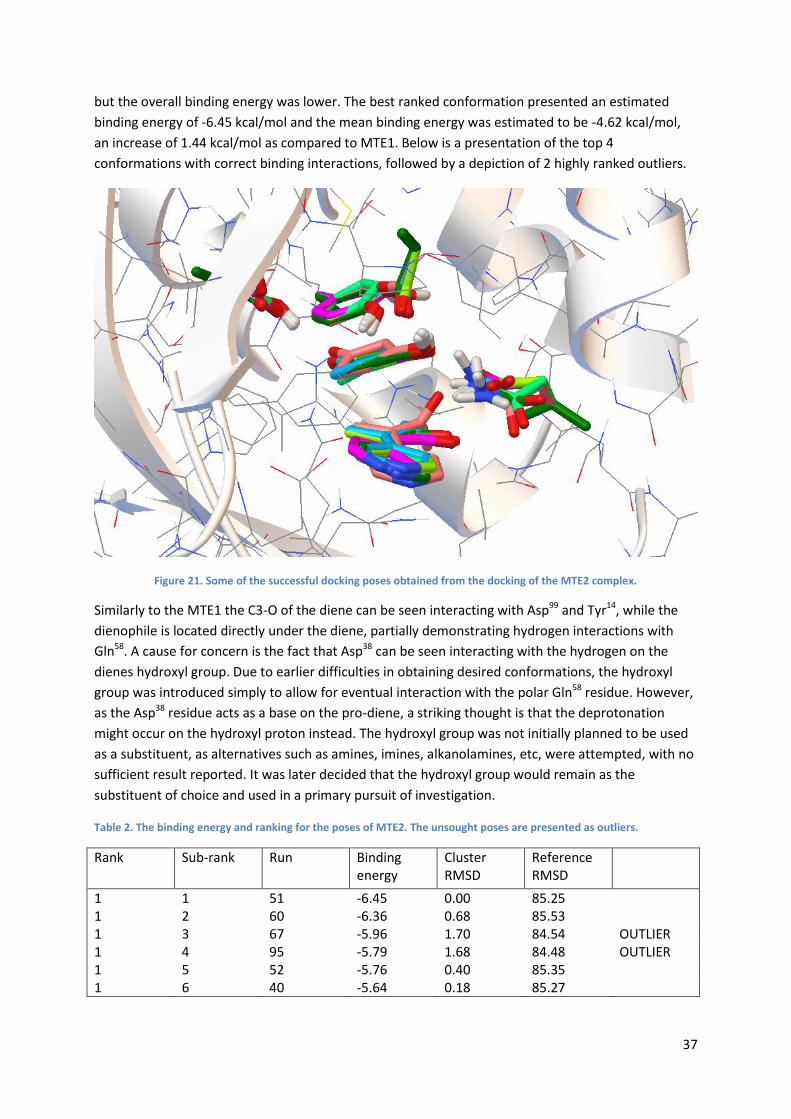
37

but the overall binding energy was lower. The best ranked conformation presented an estimated

binding energy of -6.45 kcal/mol and the mean binding energy was estimated to be -4.62 kcal/mol,

an increase of 1.44 kcal/mol as compared to MTE1. Below is a presentation of the top 4

conformations with correct binding interactions, followed by a depiction of 2 highly ranked outliers.

Figure 21. Some of the successful docking poses obtained from the docking of the MTE2 complex.

Similarly to the MTE1 the C3-O of the diene can be seen interacting with Asp99 and Tyr14, while the

dienophile is located directly under the diene, partially demonstrating hydrogen interactions with

Gln58. A cause for concern is the fact that Asp38 can be seen interacting with the hydrogen on the

dienes hydroxyl group. Due to earlier difficulties in obtaining desired conformations, the hydroxyl

group was introduced simply to allow for eventual interaction with the polar Gln58 residue. However,

as the Asp38 residue acts as a base on the pro-diene, a striking thought is that the deprotonation

might occur on the hydroxyl proton instead. The hydroxyl group was not initially planned to be used

as a substituent, as alternatives such as amines, imines, alkanolamines, etc, were attempted, with no

sufficient result reported. It was later decided that the hydroxyl group would remain as the

substituent of choice and used in a primary pursuit of investigation.

Table 2. The binding energy and ranking for the poses of MTE2. The unsought poses are presented as outliers.

Rank Sub-rank Run Binding energy

Cluster RMSD

Reference RMSD

1 1 51 -6.45 0.00 85.25 1 2 60 -6.36 0.68 85.53 1 3 67 -5.96 1.70 84.54 OUTLIER 1 4 95 -5.79 1.68 84.48 OUTLIER 1 5 52 -5.76 0.40 85.35 1 6 40 -5.64 0.18 85.27

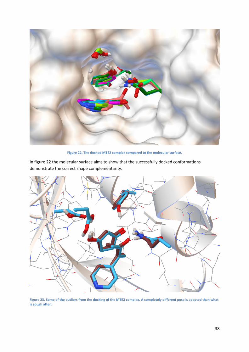
38

Figure 22. The docked MTE2 complex compared to the molecular surface.

In figure 22 the molecular surface aims to show that the successfully docked conformations

demonstrate the correct shape complementarity.

Figure 23. Some of the outliers from the docking of the MTE2 complex. A completely different pose is adapted than what is sough after.

39

Figure 23 and 24 presents some of the outliers obtained within the rank 1 cluster where the expected

interactions are not present. Likely this is due to the added methyl group on the carbonyl of the

diene causing the structure to explore other conformations, allowing more room for the compound.

The figure depicting the molecular surface illustrates that the rational design possibly could have

rendered the active site too small for a structure with an added methyl group.

Figure 24. The outliers of MTE2 complared to the molecular surface.

The next structure explored the option of adding a methyl group on the pyridine substituent, next to

the nitrogen. Remaining true to the earlier naming conventions, this structure is denoted as MTE3.

Figure 25. The structure of the MTE3 complex is presented. A methyl group has been added to the pyridine group.

40

For the MTE3 TS-structure, 100 GA runs were performed, (as for MTE2) generating an overall

increase in binding energy but fewer numbers of conformations present in the rank 1 cluster. The

best conformation demonstrated an estimated binding energy of -6.74 kcal/mol and the mean

binding energy was -4.64 kcal/mol (a poor -0.02 kcal/mol lower compared to MTE2). Out of 7

reported clusters, the rank 1 cluster contained 61 conformations, meaning that fewer conformations

were obtained. The figures below show the 8 best ranked conformations, energy-wise. However, 4

out of these top ranked conformations were deemed to be outliers.

Figure 26. The successfully obtained docking poses for MTE3.

Figure 26 demonstrates the obtained conformations that fulfilled the interactions criteria, but with a

slightly increased variation in positioning even for seemingly equal conformations and figure 27 show

the molecular surface. An estimated guess is that the methyl group added to the pyridine substituent

serves to increase the hydrophobic interactions, while the methyl group on the carbonyl group can

cause certain distortions as a result of steric clashes, which might explain the conformational

variation observed for MTE2.

Table 3. The binding energies and subsequent rankings of poses. Outliers are presented as well.

Rank Sub-rank Run Binding energy

Cluster RMSD

Reference RMSD

1 1 92 -6.74 0.00 85.21 1 2 32 -6.63 1.66 84.66 OUTLIER 1 3 13 -6.39 1.69 84.60 OUTLIER 1 4 18 -6.05 1.03 85.02 OUTLIER 1 5 5 -6.05 1.82 84.77 1 6 60 -6.04 0.74 84.89 1 7 33 -6.01 1.12 85.50 1 8 29 -5.74 1.69 84.30 OUTLIER

41

Figure 27. The successful dockings of MTE3 compared to the molecular surface.

In figure 28 and 29 below, the outliers for MTE3 are presented. Due to restricted access of space in

the active site the TS-structure attempts to explore different conformations by twisting itself into

more fitting poses. This early on led to the belief that further addition of substituents to the complex

would result in it being too large to even enter the site, or at least, not providing the sought after

binding interactions. The assumption would prove, as results will show, to be fairly correct.

Figure 28. Outliers obtained from the MTE3 docking.

42

Figure 29. The outliers for MTE3 compared to the molecular surface.

The last investigated TS-structure is presented below, where the main purpose was to determine if

the substrate design was pushing the limits in regards to steric clashes with the residues in the active

site. The complex is denoted as MTE4.

Figure 30. The representation for the MTE4 complex.

Like MTE2 and MTE3, MTE4 was subjected to 100 GA runs, generating a considerably lower binding

energy overall, but a variety of clusters with the rank 1 and rank 2 clusters, containing 35

conformations each. Some samples are presented in figure 31 to demonstrate the inability of the

designed complex to achieve the desired binding interactions. As no correct binding interactions

were detected out of all 100 generated conformations, there is no need for a presentation of the

binding energies. In figure 32 which presents the sampled conformation along with the molecular

surface, the conformation with bold bonds is shown as an interesting comparison in relation to the

43

others. A new conformation not previously detected is presented, where the pyridine group is

twisted to fit the complex into the active site. A quick conclusion can be drawn from simple visual

inspection that the MTE4 complex is too large for the active site, resulting in the absence of the

necessary interactions that leads to catalysis.

Figure 31. The MTE4 complex showed no favorable interactions whatsoever and was therefore removed from further consideration and evaluation as a plausible substrate design.

Figure 32. The MTE4 complex compared to the molecular surface. The bold representations demonstrate that the complex explored new conformations, yet to have been seen before.

44

The MTE1, MTE2 and MTE3 complexes were chosen to be evaluated with molecular dynamics.

Complete cluster analysis can be found in Appendix 2.

4.2 Evaluation with Molecular Dynamics Based on previous work conducted by Brinck et al [43] the focus in the MD simulations rests on

studying the specific binding interactions of the ligand towards the catalytic residues in the active

site. The results presented here can only be considered as the tip of the iceberg in regards to

determine if the substrate and active site design was sufficient enough. As described in their work,

the so called ‘near attack conformers’ (NAC) for a D-A reaction can be viewed as an overlap between

the diene and dienophile, where the free energy of activation is determined by the ability of the

ligand to go from the bound state to NAC and thereafter from NAC to TS. Basically, this means that

the structure should retain its interactions with the residues necessary for catalysis to take place,

while simultaneously maintaining the interacting relationship between a diene and dienophile. As no

MD simulations was performed for the diene and dienophile by themselves, but only for the poses

obtained from docking the TS-structure, the free energy of activation could not be determined.

Therefore, this section relied on visual inspection only, where a 4 ns simulation was performed for

MTE1, MTE2 and MTE3, respectively. A 10 ns simulation was conducted for MTE1 and MTE3 as well

to see if eventual change occurred later during the simulation, which might tell of eventual

interesting behavior. Seeing as this is the case, the only important conclusion that could be drawn

from this initial investigation was whether the active site design was sufficient enough to contain the

diene and dienophile in an organized state. Namely, could the active site preserve the poses

obtained from the docking stage within the limits off a TS-like configuration?

4.2.1 MD simulation of MTE1

The results obtained from the molecular docking of MTE1 showed good promise as candidates for

the MD simulation. However, during the MD simulation it became apparent that the complex worked

poorly for the active site design. Following just a few ps into the simulation the dienophile showed

signs of leaving the site, indicating that the design was not feasible. Following is a presentation of the

system at 0, 1 and 10 ns respectively. The simulation at 10 ns is presented to demonstrate the

instability of the design.

45

Figure 33. MTE1 at 0 ns. The NACs are still maintained and this type of positioning of the TS-complex was the sought after one.

46

Figure 34. The MTE1 simulation at 1 ns. It is obvious that the dienophile is not suitable for this particular active site design. It is difficult to distinguish the exact cause of error as it might potentially lie in the substrate design but also in the active site design. It is more probable that it is the active site that is too hydrophilic and therefore cannot sustain the TS-complex for various reasons. Whereas these reasons are due to protein backbone restructuring or other issues have yet to been determined for this work.

47

Figure 35. As 10 ns has passed, the diene has maximized its hydrogen bonding interactions, while the dienophile is no longer actively participating in the active site. Due to the instability of the complex toward the active site, the complex was subsequently discarded for this particular mutant.

48

4.2.2 MD simulation of MTE2

Presented below are two figures representing the conformations interacting with the active site at

the initial stage of the MD simulation (i.e. at 0 ns) and after some eloped time (1 ns), respectively.

From figure 33 it can be seen that the diene and dienophile exist in a TS-like state, such as that

described in section 4.1.2. However, quite quickly the dienophile seemingly left its location from

beneath the diene, veering away from the active site. This can be viewed in figure 34 and although

the simulation was performed up to 4 ns, the dienophile never reclaimed its position. This indicated

that the design of MTE2 was a failure which would probably not result in a satisfactory interaction

with the active site. As such, the work with MTE2 was abandoned.

Figure 36. The starting position for the MD simulation at 0 ns. The TS-structure is still retained and the diene can be seen interacting favorable with Asp

99 and Tyr

14.

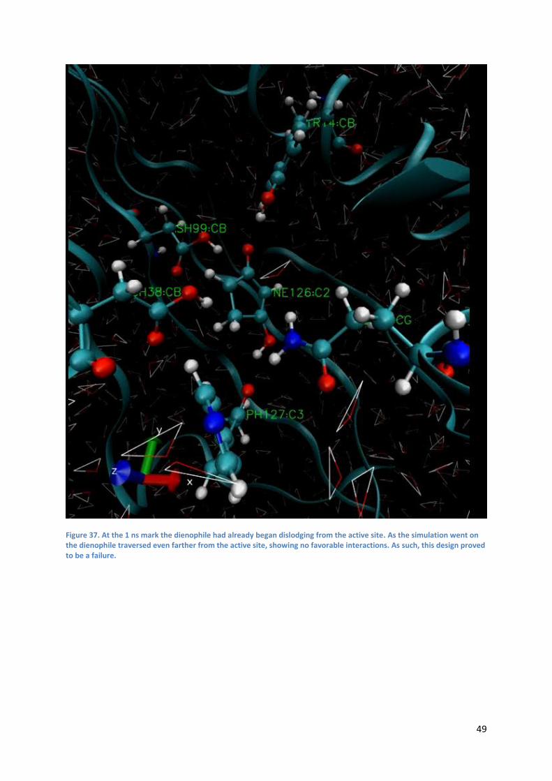
49

Figure 37. At the 1 ns mark the dienophile had already began dislodging from the active site. As the simulation went on the dienophile traversed even farther from the active site, showing no favorable interactions. As such, this design proved to be a failure.

50

4.2.3 MD simulation of MTE3

While the MTE1 and MTE2 designs had failed to retain a TS-like configuration, a different observation

was made for the MTE3 design. The following five figures presents the development of the MTE3 MD

simulation at 0, 1, 2, 3 and 4 ns, respectively. At the start of the simulation the ligands can be seen

positioned quite close to the TS-structure, with the diene maintaining a steady interaction with both

Asp99 and Tyr14. As the simulation approaches 1 ns the hydroxyl proton initiates interaction with an

approaching water molecule, which appears to be tilting the diene a bit, although it still remains in a

steadfast interaction with Asp99 and Tyr14. The dienophile retains its position below the diene while

exploring different conformations, At 2 ns, both the diene and Asp38 are interacting with the water

molecule mentioned earlier and the overall system appears to be in a relatively stable state, except

for the dienophile which positions itself almost perpendicular to the diene, resulting in a temporary

dislodging from the more planar state it adopted earlier in relation to the diene. A positive aspect

however, is that the dienophile seems to prevail in positioning itself directly below the diene, as

opposed to in MTE2 where it left the active site almost immediately. Approaching the 3 ns mark the

water molecule has begun to move further away from its previous position. Asp38 is now interacting

with the hydroxyl oxygen on the diene and the dienophile reclaims a more planar conformation next

to the diene. However, at 4 ns the interaction between the hydroxyl group on the diene and the

Asp38 residue has ceased, with the likely reason being that the diene has tilted away from its original

position. Even though the complex was unable in maintaining the necessary overlap for the diene

and dienophile to adopt a TS-like configuration, the complex did not reposition itself entirely. This

indicates that the designed substrate might strive to adopt a proper relative positioning, if exposed

to slight modification. It is also unfortunate that no MD simulations were conducted for the diene

and dienophile individually, as this would have enabled calculation of the free energy of binding. A

value for the free energy of binding could distinguish between a decent result and wishful thinking,

as a visual inspection will not accurately reflect the obtained result. The observation that the

complex does not explore the active site in a completely random fashion serves as a strong indication

that the main interactions are preserved. This does not confirm to what extent they are preserved

since the results depend on a visual inspection of the trajectory.

When a longer simulation (10 ns) was performed, it became obvious that even MTE3 had failed.

Passing the 3-4 ns limit the dienophile became unstable in the active site and evacuated the active

site. This was a reoccuring phenomenon for each following simulation with a new random seed.

51

Figure 38. The starting coordinates obtained from the docking phase, at 0 ns during the start of the simulation.

52

Figure 39. The simulation shows stability in that the dienophile remains in its original starting position. However, the hydroxyl group on the diene can be seen interacting with a water molecule through hydrogen bonding, which would eventually lead to the compound becoming slightly tilted.

53

Figure 40. 2 ns into the simulation and both diene and dienophile remain within close border of the starting coordinates. As mentioned earlier in figure 36, the hydroxyl group demonstrates interactions with a single water molecule. This is also true for Asp

38, showing some interactions with the water molecule. As no further calculations was performed beyond

this point it is difficult to ascertain if the complex is of good of poor design, although it shows promise.

54

Figure 41. This figure shows the simulation at 3 ns and it is clear that the diene has tilted to the side a bit. The overlapping effect between diene and dienophile is not excellent, but both molecules are retaining important interactions within the active site.

55

Figure 42. At the 4 ns mark the diene is seen clearly tilted. The overlap between the diene and dienophile is fairly poor, but in contrast to what has been reported in previous work [5][43] regarding catalytic antibodies, designed to catalyze the D-A reaction, the molecules do not adapt random interactions within the active site. A possible conclusion to be drawn from this is that even though Siegel and co-workers managed catalysis with molecules adapting random conformations, with a quite low catalytic activity, the pre-organization of the enzyme for this particular substrate is not too poor. This indicates that with some minor design revision, the suggested mutant and substrate might produce a fair result. But since the dienophile showed instability after 4 ns one might suggest that the active site design is not optimal for this particular substrate, and that the pyridine group used as a substituent might be a fair guess if screened towards a different mutant.

56

5. Conclusion This work has demonstrated that by employing the protocol developed by Brinck et al [8][43], it is

possible to employ rational design in order to enhance the capabilities of enzymes. Although no

specific substrate or active site design could be accurately determined, some insight was gained of

which residues could be utilized for design purposes to enhance the binding energy, while

simultaneously providing an increased frequency of optimal conformations. By investigating different

substitution patterns on the diene and dienophile, a notable increase in binding affinity and

consistent binding interactions was observed in the wildtype KSI as well, as compared to the initial

trial dockings conducted with the scaffold TS-structures presented in figure 7. This serves as a good

indication that by generating an appropriate design of a substrate, a D-A reaction could readily be

performed in native KSI. The optimal increase in enzyme-substrate affinity is obtained by focusing on

designing the substrates in concert with one another. This increase is ascribed to the enzymes ability

to organize the substrates in a fashion that allows an easier access to the TS. This has been described

earlier and is enforced by the result of the early state MD (<4 ns) of the MTE3 complex.

The use of pyridine as a potential substituent cannot be excluded, as it provided overall positive

results, no matter what environment it was evaluated in. The pyridine substituent allows for

potential hydrogen bonding as well as pi-pi interactions with the prevalent aromatic side chains in

the active site. However, the redesign of the active site most likely has to take a different turn. A

longer evaluation of the MTE1 and MTE3 complexes (up to 10 ns), with a random seed, showed no

improvement whatsoever in regards to the stability of the complex. For the MTE1 complex, the

dienophile left the active site within the scope of 1 ns, and the MTE3 complex simulations managed a

stable enough positioning in the active site for up to 3-4 ns. Each mutant protein was relaxed before

molecular docking and molecular dynamics simulations were conducted, and the active site did not

demonstrate a large distortion in either case, compared to the wild type KSI. But since no actual

RMSD comparisons were conducted, and the backbone distortion was only visually inspected, it

poses a problem when one has to qualitatively discuss the problem of introduced mutations effect

on the protein backbone structure. The relaxation of the mutants was conducted mainly to

investigate that the active site did not collapse on itself upon introduction of new side chains, and to

obtain as thorough docking results as possible.

The introduction of more hydrophilic side chains may initially have provided an enhanced binding

affinity and a good pre-organization of the TS-complex. But the question remains to see if this

actually prevails. It can be argued that introducing hydrophilic residues into such a hydrophobic site,

such as in KSI, is counterproductive. It allows for the introduction of several possible hydrogen bonds,

but one of the characteristics for KSI is the pKa of the Asp99 and Asp38, which has shown to be

dependent on the hydrophobic environment [9][11]. While the introduction of hydrogen bonding

capabilities might affect the binding affinity positively, it is difficult to properly evaluate the exact

influence this will have on the reaction at a later stage. The eventual shift in pKa values might turn

out to decrease the catalytic efficiency, while the binding affinity is demonstrated to be potentially

quite favorable.

It can thus be concluded that the pyridine substituent might be a quite valuable choice, whereas the

hydroxyl group on the diene is a cause for concern due to eventual deprotonization. But with a

proper redesign of the active site, with introduction of several hydrophobic side chains, and also one

or more hydrophobic substituents on the diene, the hydrophobic interactions could plausibly be fully

57

utilized, while retaining a proper pre-organization of the TS-complex and avoiding a larger shift in the

pKa of the vitally important catalytic triad.

A concluding remark on how to speed up the screening process, which also may include more

frequent hits using the AutoDock set of programs, will follow. As the results suggest that some

particular structures are favorable to others, one might consider utilizing AutoDock Vina [44] for a

quicker initial virtual screening of compounds. Due to the difference in scoring tactics utilized in Vina

and AD4, Vina could screen large libraries of substituted TS-structures (as no incorporated charge

parameter is included Vina performs faster calculations) and focus on shape complementarity, while

AD4 could be employed when hits have been discovered with Vina, subsequently incorporating a

charge parameter. As the TS-structure is reliant on the emerging anionic charge, the structural fit

would allow for the organization of diene and dienophile, hopefully maximizing the overlap between

the two compounds. An additional property that is invaluable to the increased efficiency of the

virtual screening process lies in the speed of the virtual screening process. Not simply in regards to

the screening of ligands towards the wild type protein, but also when trying out different mutations.

This results in a simple workflow where the ligand library is screened towards the wild type protein,

the wild type is mutated and the most successful hits are screened against the different mutants.

Preferably the mutations will be performed with the same side chain each time, until one mutation is

deemed the best. From there, one can evaluate continued mutations swiftly with Vina, until a set of

mutants are obtained with several newly incorporated side chains. It would probably be wise to set a

binding affinity threshold for the virtually screened compounds as an initial guideline regarding the

mutations.

58

References

1. Nguyen, L.A., He, H. & Pham-Huy, C., 2006. Chiral drugs: an overview. International

journal of biomedical science : IJBS, 2(2), pp.85–100. Available at:

http://www.ncbi.nlm.nih.gov/pubmed/17221858.

2. Diels, O. & Alder, K,.1928. Justus Liebigs Ann. Chem. 460, pp. 98-122.

3. Borman, S., 2001. ASYMMETRIC CATALYSIS WINS. Chemical & Engineering

News, 79(42), pp.5–6. Available at:

http://pubs.acs.org/cen/topstory/7942/7942notw1.html.

4. Röthlisberger, D. et al., 2008. Kemp elimination catalysts by computational enzyme

design. Nature, 453(7192), pp.190–195. Available at:

http://www.ncbi.nlm.nih.gov/pubmed/18354394.

5. Siegel, J.B. et al., 2010. Computational Design of an Enzyme Catalyst for a

Stereoselective Bimolecular Diels-Alder Reaction. Science, 329(5989), pp.309–313.

Available at: http://www.sciencemag.org/cgi/doi/10.1126/science.1190239.

6. Zanghellini, A. et al., 2006. New algorithms and an in silico benchmark for

computational enzyme design. Protein Science, 15(12), pp.2785–2794. Available at:

http://doi.wiley.com/10.1110/ps.062353106.

7. Linder, M. et al., 2012. Envisioning an enzymatic Diels–Alder reaction by in situ

acid–base catalyzed diene generation. Chemical Communications, 48(45), p.5665.

Available at: http://www.ncbi.nlm.nih.gov/pubmed/22547054.

8. Linder, M. et al., 2011. Designing a New Diels–Alderase: A Combinatorial,

Semirational Approach Including Dynamic Optimization. Journal of Chemical

Information and Modeling, 51(8), pp.1906–1917. Available at:

http://pubs.acs.org/doi/abs/10.1021/ci200177d.

9. Ha, N.C. et al., 2001. Structure and enzymology of Delta5-3-ketosteroid isomerase.

Current opinion in structural biology, 11(6), pp.674–8. Available at:

http://www.ncbi.nlm.nih.gov/pubmed/11751047.

10. Sharma, K., Vázquez-Ramírez, R. & Kubli-Garfias, C., 2006. A theoretical model of

the catalytic mechanism of the Δ5-3-ketosteroid isomerase reaction. Steroids, 71(7),

pp.549–557. Available at:

http://linkinghub.elsevier.com/retrieve/pii/S0039128X05002801.

11. Cho, H.-S. et al., 1999. Crystal Structure of 5-3-Ketosteroid Isomerase from

Pseudomonas testosteroni in Complex with Equilenin Settles the Correct Hydrogen

Bonding Scheme for Transition State Stabilization. Journal of Biological Chemistry,

274(46), pp.32863–32868. Available at:

http://www.jbc.org/cgi/doi/10.1074/jbc.274.46.32863.

12. Pollack, R.M., 2004. Enzymatic mechanisms for catalysis of enolization: ketosteroid

isomerase. Bioorganic Chemistry, 32(5), pp.341–353. Available at:

http://linkinghub.elsevier.com/retrieve/pii/S0045206804000550.

13. Schwans, J.P., Kraut, D.A. & Herschlag, D., 2009. Determining the catalytic role of

remote substrate binding interactions in ketosteroid isomerase. Proceedings of the

National Academy of Sciences, 106(34), pp.14271–14275. Available at:

http://www.pnas.org/content/106/34/14271.full.

14. Clayden, J. et al., 2001. Organic Chemistry, Available at:

http://books.google.com/books?id=Dy5-vEst37oC&pgis=1.

15. Kuntz, I. D., et al. (1982). A geometric approach to macromolecule-ligand

interactions. J Mol Biol 161(2), pp. 269-288.

59

16. Sousa, S.F., Fernandes, P.A. & Ramos, M.J., 2006. Protein-ligand docking: Current

status and future challenges. Proteins: Structure, Function, and Bioinformatics, 65(1),

pp.15–26. Available at: http://doi.wiley.com/10.1002/prot.21082.

17. Sousa, S.F. et al., 2013. Protein-Ligand Docking in the New Millennium – A

Retrospective of 10 Years in the Field. Current Medicinal Chemistry, 20(18),

pp.2296–2314. Available at: http://www.ncbi.nlm.nih.gov/pubmed/23531220.

18. Morris, G.M. et al., 1998. Automated docking using a Lamarckian genetic algorithm

and an empirical binding free energy function. Journal of Computational Chemistry,

19(14), pp.1639–1662. Available at: http://doi.wiley.com/10.1002/%28SICI%291096-

987X%2819981115%2919%3A14%3C1639%3A%3AAID-JCC10%3E3.0.CO%3B2-

B.

19. Berg, J.M., Tymoczko, J.L. & Stryer, L., 2012. Biochemistry.

20. Carlson, H.A., 2002. Protein flexibility is an important component of structure-based

drug discovery. Curr Pharm Des, 8(17), pp.1571–1578. Available at:

http://www.ncbi.nlm.nih.gov/entrez/query.fcgi?cmd=Retrieve&db=PubMed&dopt=Ci

tation&list_uids=12052201.

21. Huey, R. et al., 2007. Software news and update a semiempirical free energy force

field with charge-based desolvation. Journal of Computational Chemistry, 28(6),

pp.1145–1152.

22. Weiner, S. et al., 1984. A new force field for molecular mechanical simulation of

nucleic acids and proteins. Journal of the American Chemical Society. Available at:

http://pubs.acs.org/cgi-bin/abstract.cgi/jacsat/1984/106/i03/f-

pdf/f_ja00315a051.pdf?sessid=6006l3.

23. Appleman, P., 2000. Darwin.

24. Solis, F.J. & Wets, R.J.B., 1981. Minimization by Random Search Techniques.

Mathematics of Operations Research, 6, pp.19–30.

25. Leach, A.R., 2001. Molecular Modelling: Principles and Applications,

26. Szabo, A. & Ostlund, N.S., 1996. Modern Quantum Chemistry: Introduction to

Advanced Electronic Structure Theory, Available at:

http://www.amazon.com/Modern-Quantum-Chemistry-Introduction-

Electronic/dp/0486691861.

27. Schrödinger, E., 1926. Quantisierung als Eigenwertproblem. Annalen der Physik,

384(4), pp.489–527. Available at: http://doi.wiley.com/10.1002/andp.19263840404.

28. Burke, K., 2012. Perspective on density functional theory. The Journal of Chemical

Physics, 136(15), p.150901. Available at:

http://www.ncbi.nlm.nih.gov/pubmed/22519306.

29. Becke, A.D., 2014. Perspective: Fifty years of density-functional theory in chemical

physics. The Journal of Chemical Physics, 140(18), p.18A301. Available at:

http://www.ncbi.nlm.nih.gov/pubmed/24832308\nhttp://scitation.aip.org/content/aip/jo

urnal/jcp/140/18/10.1063/1.4869598.

30. Hohenberg, P.; Kohn, W., 1964. Hohenberg, P.; Kohn, W. Phys. Rev., 136, pp.B864–

B871.

31. Johnson, K.H., 1973. Scattered-Wave Theory of the Chemical Bond. Advances in

Quantum Chemistry, 7(C), pp.143–185.

32. Becke, A.D., 1993. Density-functional thermochemistry. III. The role of exact

exchange. The Journal of Chemical Physics, 98(7), p.5648. Available at:

http://link.aip.org/link/JCPSA6/v98/i7/p5648/s1&Agg=doi\nhttp://scitation.aip.org/co

ntent/aip/journal/jcp/98/7/10.1063/1.464913.

33. Zhao, Y. & Truhlar, D.G., 2008. The M06 suite of density functionals for main group

thermochemistry, thermochemical kinetics, noncovalent interactions, excited states,

60

and transition elements: two new functionals and systematic testing of four M06-class

functionals and 12 other function. Theoretical Chemistry Accounts, 120(1-3), pp.215–

241. Available at: http://link.springer.com/10.1007/s00214-007-0310-x.

34. Case, D.A. et al., 2014. Amber 14. University of California, San Francisco, (January).

Available at: http://ambermd.org/.

35. Maier, J.A. et al., 2015. ff14SB: Improving the Accuracy of Protein Side Chain and

Backbone Parameters from ff99SB. Journal of Chemical Theory and Computation,

11, pp.3696–3713. Available at: http://pubs.acs.org/doi/abs/10.1021/acs.jctc.5b00255.

36. Wang, J. et al., 2004. Development and testing of a general Amber force field. Journal

of Computational Chemistry, 25(9), pp.1157–1174.

37. Wang, J. et al., 2005. Antechamber, An Accessory Software Package For Molecular

Mechanical Calculations. Journal of computational chemistry, 25(2), pp.1157–1174.

38. Wang, J. et al., 2006. Automatic atom type and bond type perception in molecular

mechanical calculations. Journal of Molecular Graphics and Modelling, 25(2),

pp.247–260.

39. Cornell, W.D. et al., 1993. Application of RESP Charges To Calculate Conformational

Energies, Hydrogen Bond Energies, and Free Energies of Solvation. Journal of the

American Chemical Society, 115(7), pp.9620–9631.

40. Mark, P. & Nilsson, L., 2001. Structure and dynamics of the TIP3P, SPC, and SPC/E

water models at 298 K. Journal of Physical Chemistry A, 105(43), pp.9954–9960.

41. G??tz, A.W. et al., 2012. Routine microsecond molecular dynamics simulations with

AMBER on GPUs. 1. generalized born. Journal of Chemical Theory and

Computation, 8(5), pp.1542–1555.

42. Morris, G.M. et al., 2009. Software news and updates AutoDock4 and

AutoDockTools4: Automated docking with selective receptor flexibility. Journal of

Computational Chemistry, 30(16), pp.2785–2791.

43. Linder, M. et al., 2012. Computational design of a Diels–Alderase from a thermophilic

esterase: the importance of dynamics. Journal of Computer-Aided Molecular Design,

26(9), pp.1079–1095. Available at: http://link.springer.com/10.1007/s10822-012-

9601-y.

44. Trott, O. & Olson, A.J., 2010. AutoDock Vina. J. Comput. Chem., 31, pp.445–461.

61

Appendix 1

Figure A.1. The suggested flowchart developed by Brinck and co-workers, upon which this work has been based on.

62

Figure A.2. A sample of some of the attempted substitutions for the substrate design.

63

Appendix 2

MTE1 – Cluster analysis of conformations CLUSTER ANALYSIS OF CONFORMATIONS

_________________________________

Number of conformations = 50

RMSD cluster analysis will be performed using the ligand atoms only (18 / 48 total atoms).

Outputting structurally similar clusters, ranked in order of increasing energy.

________________________________________________________________________________

Number of distinct conformational clusters found = 6, out of 50 runs,

Using an rmsd-tolerance of 2.0 A

CLUSTERING HISTOGRAM

____________________

________________________________________________________________________________

Cluster rank

Lowest Binding Energy

Run

Mean Binding Energy

Number in Cluster

Histogram

_______________________________________________________________________________

1 | -7.21 | 42 | -6.06 | 28 |############################

2 | -6.27 | 20 | -5.51 | 2 |##

3 | -6.13 | 17 | -5.31 | 15 |###############

4 | -5.15 | 18 | -5.14 | 2 |##

5 | -4.69 | 27 | -4.62 | 2 |##

6 | -4.07 | 48 | -4.07 | 1 |#

_____|___________|_____|___________|_____|______________________________________

Number of multi-member conformational clusters found = 5, out of 50 runs.

RMSD TABLE

__________

64

Rank Sub-rank Run Binding energy

Cluster RMSD

Reference RMSD

Grep Pattern

1 1 42 -7.21 0.00 85.19 RANKING

1 2 14 -6.91 0.70 85.59 RANKING

1 3 47 -6.90 0.40 85.30 RANKING

1 4 40 -6.67 0.26 85.30 RANKING

1 5 44 -6.65 0.53 85.32 RANKING

1 6 29 -6.54 0.23 85.27 RANKING

1 7 43 -6.51 0.22 85.23 RANKING

1 8 46 -6.47 0.56 85.19 RANKING

1 9 23 -6.36 0.41 85.25 RANKING

1 10 3 -6.35 0.17 85.16 RANKING

1 11 38 -6.29 0.50 85.22 RANKING

1 12 12 -6.18 1.57 85.52 RANKING

1 13 49 -6.10 0.65 85.46 RANKING

1 14 8 -6.08 1.38 85.12 RANKING

1 15 37 -6.08 1.39 84.90 RANKING

1 16 35 -6.04 0.43 85.23 RANKING

1 17 16 -6.04 0.36 85.39 RANKING

1 18 34 -5.88 1.45 84.82 RANKING

1 19 30 -5.87 0.68 85.44 RANKING

1 20 7 -5.85 0.78 85.21 RANKING

1 21 33 -5.69 1.59 85.15 RANKING

1 22 1 -5.59 0.53 85.46 RANKING

1 23 2 -5.56 0.77 85.77 RANKING

1 24 39 -5.55 0.89 85.68 RANKING

1 25 21 -5.39 1.49 85.34 RANKING

65

1 26 10 -5.38 1.51 85.24 RANKING

1 27 25 -5.34 1.55 85.39 RANKING

1 28 4 -4.21 1.19 85.57 RANKING

2 1 20 -6.27 0.00 86.17 RANKING

2 2 15 -4.75 1.97 86.15 RANKING

3 1 17 -6.13 0.00 85.15 RANKING

3 2 36 -5.98 1.49 85.50 RANKING

3 3 6 -5.71 1.58 84.32 RANKING

3 4 28 -5.47 1.63 84.67 RANKING

3 5 5 -5.46 1.53 84.82 RANKING

3 6 32 -5.31 1.09 85.06 RANKING

3 7 24 -5.29 1.54 84.82 RANKING

3 8 19 -5.29 1.86 85.24 RANKING

3 9 31 -5.10 1.12 85.00 RANKING

3 10 22 -5.09 1.39 84.54 RANKING

3 11 13 -5.08 1.86 85.32 RANKING

3 12 9 -5.02 1.27 84.47 RANKING

3 13 26 -4.99 1.38 84.31 RANKING

3 14 41 -4.88 1.54 85.06 RANKING

3 15 50 -4.85 1.76 84.16 RANKING

4 1 18 -5.15 0.00 85.50 RANKING

4 2 11 -5.13 0.48 85.50 RANKING

5 1 27 -4.69 0.00 84.68 RANKING

5 2 45 -4.56 0.69 84.45 RANKING

6 1 48 -4.07 0.00 85.44 RANKING

MTE2 – Cluster analysis of conformations CLUSTER ANALYSIS OF CONFORMATIONS

66

_________________________________

Number of conformations = 100

RMSD cluster analysis will be performed using the ligand atoms only (19 / 49 total atoms).

Outputting structurally similar clusters, ranked in order of increasing energy.

________________________________________________________________________________

Number of distinct conformational clusters found = 7, out of 100 runs,

Using an rmsd-tolerance of 2.0 A

CLUSTERING HISTOGRAM

____________________

Cluster rank

Lowest Binding Energy

Run

Mean Binding Energy

Number in Cluster

Histogram

_______________________________________________________________________________

1 | -6.45 | 51 | -4.62 | 73 |#######################################

| | | | |##################################

2 | -4.94 | 47 | -4.84 | 3 |###

3 | -4.59 | 96 | -3.60 | 7 |#######

4 | -4.12 | 82 | -3.20 | 5 |#####

5 | -3.56 | 46 | -2.89 | 8 |########

6 | -3.14 | 39 | -3.14 | 1 |#

7 | -2.82 | 45 | -2.32 | 3 |###

_____|___________|_____|___________|_____|______________________________________

Number of multi-member conformational clusters found = 6, out of 100 runs.

RMSD TABLE

__________

Rank Sub-rank Run Binding energy

Cluster RMSD

Reference RMSD

Grep Pattern

_____________________________________________________________________

1 1 51 -6.45 0.00 85.25 RANKING

67

1 2 60 -6.36 0.68 85.53 RANKING

1 3 67 -5.96 1.70 84.54 RANKING

1 4 95 -5.79 1.68 84.48 RANKING

1 5 52 -5.76 0.40 85.35 RANKING

1 6 40 -5.64 0.18 85.27 RANKING

1 7 22 -5.55 0.46 85.29 RANKING

1 8 98 -5.52 0.26 85.28 RANKING

1 9 28 -5.47 1.81 84.35 RANKING

1 10 41 -5.47 1.49 84.95 RANKING

1 11 18 -5.45 0.47 85.33 RANKING

1 12 33 -5.38 0.38 85.37 RANKING

1 13 10 -5.38 0.32 85.33 RANKING

1 14 76 -5.33 1.40 85.40 RANKING

1 15 68 -5.28 1.78 84.30 RANKING

1 16 55 -5.27 0.44 85.33 RANKING

1 17 64 -5.26 0.39 85.24 RANKING

1 18 99 -5.22 1.74 84.75 RANKING

1 19 5 -5.19 1.80 84.50 RANKING

1 20 73 -5.18 1.83 84.33 RANKING

1 21 12 -5.12 1.38 85.16 RANKING

1 22 31 -5.12 1.77 84.41 RANKING

1 23 44 -5.10 1.83 84.31 RANKING

1 24 89 -5.03 1.42 84.92 RANKING

1 25 37 -5.03 1.77 84.38 RANKING

1 26 59 -5.02 1.00 85.26 RANKING

1 27 72 -4.98 1.70 84.42 RANKING

1 28 16 -4.89 1.39 85.18 RANKING

68

1 29 49 -4.89 1.68 85.48 RANKING

1 30 57 -4.85 0.57 85.56 RANKING

1 31 54 -4.84 1.15 85.13 RANKING

1 32 14 -4.80 0.79 85.04 RANKING

1 33 91 -4.79 1.72 84.72 RANKING

1 34 88 -4.79 1.40 85.06 RANKING

1 35 58 -4.78 0.87 84.37 RANKING

1 36 2 -4.77 1.75 84.39 RANKING

1 37 93 -4.77 0.54 85.41 RANKING

1 38 71 -4.75 1.84 84.80 RANKING

1 39 79 -4.69 1.60 84.55 RANKING

1 40 15 -4.62 1.75 84.38 RANKING

1 41 8 -4.51 1.87 84.35 RANKING

1 42 100 -4.49 1.45 85.14 RANKING

1 43 85 -4.48 0.68 85.35 RANKING

1 44 80 -4.43 1.54 85.89 RANKING

1 45 13 -4.42 0.79 85.75 RANKING

1 46 29 -4.42 1.48 84.81 RANKING

1 47 20 -4.38 0.84 85.63 RANKING

1 48 75 -4.37 0.46 85.23 RANKING

1 49 1 -4.35 1.53 86.09 RANKING

1 50 26 -4.35 1.47 84.81 RANKING

1 51 38 -4.27 1.45 84.80 RANKING

1 52 84 -4.20 1.47 84.82 RANKING

1 53 3 -4.12 1.62 85.86 RANKING

1 54 11 -4.07 1.53 84.82 RANKING

1 55 81 -3.94 1.34 85.64 RANKING

69

1 56 34 -3.87 1.98 85.74 RANKING

1 57 69 -3.82 0.50 85.34 RANKING

1 58 24 -3.81 0.52 85.26 RANKING

1 59 30 -3.79 1.42 85.87 RANKING

1 60 50 -3.77 0.67 85.36 RANKING

1 61 19 -3.68 0.51 85.27 RANKING

1 62 78 -3.64 0.59 85.29 RANKING

1 63 62 -3.63 1.47 86.09 RANKING

1 64 36 -3.62 0.57 85.35 RANKING

1 65 53 -3.61 1.14 85.36 RANKING

1 66 6 -3.60 0.57 85.27 RANKING

1 67 66 -3.58 1.59 86.07 RANKING

1 68 92 -3.54 1.16 85.72 RANKING

1 69 86 -3.45 1.28 85.53 RANKING

1 70 63 -3.35 1.64 86.12 RANKING

1 71 90 -3.30 0.71 85.55 RANKING

1 72 83 -2.99 1.55 85.74 RANKING

1 73 48 -2.99 1.65 84.58 RANKING

2 1 47 -4.94 0.00 85.99 RANKING

2 2 42 -4.86 0.35 85.89 RANKING

2 3 27 -4.72 0.24 86.00 RANKING

3 1 96 -4.59 0.00 85.12 RANKING

3 2 61 -3.84 1.33 84.56 RANKING

3 3 56 -3.42 1.08 84.70 RANKING

3 4 25 -3.40 1.57 84.23 RANKING

3 5 77 -3.36 1.37 85.30 RANKING

3 6 74 -3.34 1.82 84.81 RANKING

70

3 7 32 -3.24 1.90 84.33 RANKING

4 1 82 -4.12 0.00 85.41 RANKING

4 2 7 -3.84 0.19 85.31 RANKING

4 3 43 -2.96 1.82 85.08 RANKING

4 4 35 -2.80 1.49 84.91 RANKING

4 5 17 -2.27 0.83 85.11 RANKING

5 1 46 -3.56 0.00 85.66 RANKING

5 2 23 -3.13 0.50 85.61 RANKING

5 3 4 -2.99 1.52 85.56 RANKING

5 4 21 -2.97 0.97 85.51 RANKING

5 5 70 -2.86 1.67 84.97 RANKING

5 6 9 -2.80 1.25 85.36 RANKING

5 7 94 -2.70 1.88 84.28 RANKING

5 8 65 -2.13 1.85 84.60 RANKING

6 1 39 -3.14 0.00 86.31 RANKING

7 1 45 -2.82 0.00 84.15 RANKING

7 2 97 -2.08 1.91 85.11 RANKING

7 3 87 -2.04 1.06 83.69 RANKING

______________________________________________________________________

MTE3 – Cluster analysis of conformations CLUSTER ANALYSIS OF CONFORMATIONS

_________________________________

Number of conformations = 100

RMSD cluster analysis will be performed using the ligand atoms only (20 / 50 total atoms).

Outputting structurally similar clusters, ranked in order of increasing energy.

________________________________________________________________________________

71

Number of distinct conformational clusters found = 7, out of 100 runs,

Using an rmsd-tolerance of 2.0 A

CLUSTERING HISTOGRAM

____________________

Cluster rank

Lowest Binding Energy

Run

Mean Binding Energy

Number in Cluster

Histogram

1 | -6.74 | 92 | -4.64 | 61

#############################################################

2 | -5.23 | 43 | -4.26 | 16 |################

3 | -5.02 | 36 | -4.09 | 10 |##########

4 | -4.44 | 4 | -4.44 | 1 |#

5 | -4.00 | 97 | -3.39 | 8 |########

6 | -3.48 | 81 | -3.30 | 3 |###

7 | -2.83 | 17 | -2.83 | 1 |#

_____|___________|_____|___________|_____|______________________________________

Number of multi-member conformational clusters found = 5, out of 100 runs.

RMSD TABLE

__________

Rank Sub-rank Run Binding energy

Cluster RMSD

Reference RMSD

Grep Pattern

1 1 92 -6.74 0.00 85.21 RANKING

1 2 32 -6.63 1.66 84.66 RANKING

1 3 13 -6.39 1.69 84.60 RANKING

1 4 18 -6.05 1.03 85.02 RANKING

1 5 5 -6.05 1.82 84.77 RANKING

1 6 60 -6.04 0.74 84.89 RANKING

1 7 33 -6.01 1.12 85.50 RANKING

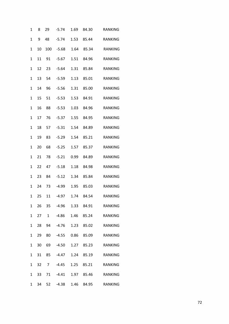
72

1 8 29 -5.74 1.69 84.30 RANKING

1 9 48 -5.74 1.53 85.44 RANKING

1 10 100 -5.68 1.64 85.34 RANKING

1 11 91 -5.67 1.51 84.96 RANKING

1 12 23 -5.64 1.31 85.84 RANKING

1 13 54 -5.59 1.13 85.01 RANKING

1 14 96 -5.56 1.31 85.00 RANKING

1 15 51 -5.53 1.53 84.91 RANKING

1 16 88 -5.53 1.03 84.96 RANKING

1 17 76 -5.37 1.55 84.95 RANKING

1 18 57 -5.31 1.54 84.89 RANKING

1 19 83 -5.29 1.54 85.21 RANKING

1 20 68 -5.25 1.57 85.37 RANKING

1 21 78 -5.21 0.99 84.89 RANKING

1 22 47 -5.18 1.18 84.98 RANKING

1 23 84 -5.12 1.34 85.84 RANKING

1 24 73 -4.99 1.95 85.03 RANKING

1 25 11 -4.97 1.74 84.54 RANKING

1 26 35 -4.96 1.33 84.91 RANKING

1 27 1 -4.86 1.46 85.24 RANKING

1 28 94 -4.76 1.23 85.02 RANKING

1 29 80 -4.55 0.86 85.09 RANKING

1 30 69 -4.50 1.27 85.23 RANKING

1 31 85 -4.47 1.24 85.19 RANKING

1 32 7 -4.45 1.25 85.21 RANKING

1 33 71 -4.41 1.97 85.46 RANKING

1 34 52 -4.38 1.46 84.95 RANKING

73

1 35 38 -4.25 1.47 85.20 RANKING

1 36 89 -4.24 1.62 85.62 RANKING

1 37 98 -4.22 1.62 84.93 RANKING

1 38 21 -4.19 1.60 85.70 RANKING

1 39 14 -4.19 1.34 85.31 RANKING

1 40 70 -4.16 1.54 84.74 RANKING

1 41 3 -4.15 1.68 85.77 RANKING

1 42 16 -4.02 1.03 85.16 RANKING

1 43 95 -3.96 1.91 85.97 RANKING

1 44 75 -3.93 1.39 85.60 RANKING

1 45 41 -3.92 1.43 85.50 RANKING

1 46 49 -3.80 1.46 85.69 RANKING

1 47 9 -3.78 1.48 85.49 RANKING

1 48 55 -3.70 1.31 84.94 RANKING

1 49 77 -3.67 1.63 85.85 RANKING

1 50 19 -3.65 1.41 85.35 RANKING

1 51 82 -3.60 1.56 85.49 RANKING

1 52 12 -3.56 1.28 84.94 RANKING

1 53 65 -3.50 1.88 85.86 RANKING

1 54 58 -3.49 1.45 85.60 RANKING

1 55 46 -3.40 1.39 85.42 RANKING

1 56 40 -3.37 1.67 85.77 RANKING

1 57 26 -3.37 1.60 85.87 RANKING

1 58 6 -3.36 1.48 85.24 RANKING

1 59 72 -3.35 1.59 85.41 RANKING

1 60 59 -3.24 1.58 85.31 RANKING

1 61 27 -2.60 1.98 85.01 RANKING

74

2 1 43 -5.23 0.00 84.66 RANKING

2 2 50 -5.20 0.40 84.66 RANKING

2 3 28 -5.16 1.00 84.81 RANKING

2 4 63 -5.01 0.43 84.62 RANKING

2 5 8 -4.58 1.00 84.48 RANKING

2 6 31 -4.57 0.86 84.81 RANKING

2 7 44 -4.50 1.04 84.47 RANKING

2 8 87 -4.41 0.97 84.44 RANKING

2 9 25 -4.41 1.00 84.41 RANKING

2 10 93 -4.17 1.97 84.72 RANKING

2 11 42 -3.74 1.93 84.34 RANKING

2 12 79 -3.73 1.92 84.34 RANKING

2 13 2 -3.71 1.28 84.59 RANKING

2 14 64 -3.66 1.35 84.93 RANKING

2 15 22 -3.06 1.98 84.38 RANKING

2 16 34 -2.94 1.96 84.43 RANKING

3 1 36 -5.02 0.00 84.57 RANKING

3 2 86 -4.87 1.09 84.59 RANKING

3 3 53 -4.53 1.21 84.66 RANKING

3 4 99 -4.33 1.15 84.58 RANKING

3 5 62 -4.29 1.19 84.69 RANKING

3 6 74 -4.27 1.20 84.37 RANKING

3 7 45 -3.61 1.21 84.67 RANKING

3 8 10 -3.49 1.14 84.54 RANKING

3 9 39 -3.33 1.14 84.21 RANKING

3 10 37 -3.21 1.64 83.87 RANKING

4 1 4 -4.44 0.00 83.87 RANKING

75

5 1 97 -4.00 0.00 85.28 RANKING

5 2 56 -3.88 1.34 85.30 RANKING

5 3 61 -3.59 1.78 85.27 RANKING

5 4 90 -3.51 1.55 85.41 RANKING

5 5 20 -3.46 0.72 85.00 RANKING

5 6 66 -3.36 1.59 85.29 RANKING

5 7 30 -2.67 1.95 84.79 RANKING

5 8 15 -2.62 1.76 85.26 RANKING

6 1 81 -3.48 0.00 84.96 RANKING

6 2 24 -3.27 0.25 84.90 RANKING

6 3 67 -3.15 0.22 84.90 RANKING

7 1 17 -2.83 0.00 84.59 RANKING

_______________________________________________________________________