Embed Size (px)
Citation preview
Computational Aspects
of DNA Copy Number
Measurement
Doron Lipson
Tec
hnio
n -
Com
pute
r Sc
ienc
e D
epar
tmen
t - P
h.D
. The
sis
PH
D-2
007-
05 -
200
7

Tec
hnio
n -
Com
pute
r Sc
ienc
e D
epar
tmen
t - P
h.D
. The
sis
PH
D-2
007-
05 -
200
7
Computational Aspects of DNA Copy
Number Measurement
Research Thesis
Submitted in partial fulfillment of the requirements
for the degree of Doctor of Philosophy
Doron Lipson
Submitted to the Senate of
the Technion — Israel Institute of Technology
Shvat 5767 Haifa February 2007
Tec
hnio
n -
Com
pute
r Sc
ienc
e D
epar
tmen
t - P
h.D
. The
sis
PH
D-2
007-
05 -
200
7

Tec
hnio
n -
Com
pute
r Sc
ienc
e D
epar
tmen
t - P
h.D
. The
sis
PH
D-2
007-
05 -
200
7

This research thesis was done under the supervision of Dr. Zohar Yakhini inthe Computer Science department.
I would like to thank Zohar Yakhini for his dedicated guidance, enthusiasticsupport and friendship throughout my studies. I am particularly gratefulfor the high degree of independence that Zohar provided, treating me as acolleague more than as a student, and for the many doors that he opened forme.
I would also like to thank the members of the Bio-Medical Assays Group atAgilent Laboratories for their collaboration on many parts of this researchproject, and for hosting me on several occasions. Specifically, I would liketo thank Amir Ben-Dor for the many fruitful discussions we had – on topicsrelated to my research and much beyond – and for his generous hospitality.
I wish to thank all collaborators who enabled this work. In particular, Iwould like to thank Yonatan Aumann for insightful discussions, which haveled to several of the main results of this thesis.
This thesis is dedicated to my wife, Adi, and my daughter, Dana, for theirlove, support, understanding and encouragement during both easy and moredifficult times.
The generous financial help of the Technion and Agilent Technologies is grate-fully acknowledged.
Tec
hnio
n -
Com
pute
r Sc
ienc
e D
epar
tmen
t - P
h.D
. The
sis
PH
D-2
007-
05 -
200
7

Tec
hnio
n -
Com
pute
r Sc
ienc
e D
epar
tmen
t - P
h.D
. The
sis
PH
D-2
007-
05 -
200
7
Contents
Abstract 1
Notation and Abbreviations 3
1 Introduction 51.1 Background . . . . . . . . . . . . . . . . . . . . . . . . . . . . 5
1.1.1 Genomic Alterations in Cancer . . . . . . . . . . . . . 51.1.2 Array-based Comparative Genomic Hybridization . . . 61.1.3 Computational Aspects of aCGH . . . . . . . . . . . . 71.1.4 Related Work . . . . . . . . . . . . . . . . . . . . . . . 11
1.2 Overview . . . . . . . . . . . . . . . . . . . . . . . . . . . . . . 15
2 Results 172.1 Design of CGH Arrays . . . . . . . . . . . . . . . . . . . . . . 17
2.1.1 Optimization of Probe Performance . . . . . . . . . . . 182.1.2 Optimization of Probe Coverage . . . . . . . . . . . . . 21
2.2 Analysis of aCGH Data . . . . . . . . . . . . . . . . . . . . . 282.2.1 Aberration Calling . . . . . . . . . . . . . . . . . . . . 282.2.2 Centering of aCGH Data . . . . . . . . . . . . . . . . . 322.2.3 Common Aberrations . . . . . . . . . . . . . . . . . . . 362.2.4 Downstream Effects of Genomic Aberrations . . . . . . 422.2.5 DNA Replication Patterns . . . . . . . . . . . . . . . . 49
2.3 Additional Results . . . . . . . . . . . . . . . . . . . . . . . . 532.3.1 Enrichment Analysis . . . . . . . . . . . . . . . . . . . 53
3 Discussion 57
Bibliography 61
Tec
hnio
n -
Com
pute
r Sc
ienc
e D
epar
tmen
t - P
h.D
. The
sis
PH
D-2
007-
05 -
200
7
A Papers 71A.1 Comparative Genomic Hybridization using Oligonucleotide Mi-
croarrays and Total Genomic DNA . . . . . . . . . . . . . . . 71A.2 Optimization of Probe Coverage for High-Resolution Oligonu-
cleotide aCGH . . . . . . . . . . . . . . . . . . . . . . . . . . . 79A.3 Efficient Calculation of Interval Scores for DNA Copy Number
Data Analysis . . . . . . . . . . . . . . . . . . . . . . . . . . . 89A.4 Determining the Center of array-CGH Data . . . . . . . . . . 105A.5 Framework for Identifying Common Aberrations in DNA Copy
Number Data . . . . . . . . . . . . . . . . . . . . . . . . . . . 111A.6 Joint Analysis of DNA Copy Numbers and Gene Expression
Levels . . . . . . . . . . . . . . . . . . . . . . . . . . . . . . . 125A.7 Discovering Motifs in Ranked Lists of DNA Sequences . . . . . 143
Tec
hnio
n -
Com
pute
r Sc
ienc
e D
epar
tmen
t - P
h.D
. The
sis
PH
D-2
007-
05 -
200
7
List of Figures
1.1 Comparative Genomic Hybridization . . . . . . . . . . . . . . 81.2 Evolution of aCGH . . . . . . . . . . . . . . . . . . . . . . . . 91.3 Aberration calls for aCGH data . . . . . . . . . . . . . . . . . 111.4 Penetrance plot . . . . . . . . . . . . . . . . . . . . . . . . . . 13
2.1 Performance of expression and CGH arrays for DNA copynumber measurement . . . . . . . . . . . . . . . . . . . . . . . 19
2.2 Parameters used for prediction of probe specificity . . . . . . . 212.3 Predictive power of the probe quality score . . . . . . . . . . . 222.4 Resolution and quality performance of UniProbe algorithm . 262.5 HD-CGH of genomic breakpoint in 17q . . . . . . . . . . . . . 272.6 Benchmarking Maximum Scoring Interval algorithms . . . . . 322.7 Significant alterations in breast cancer cell line BT-474 . . . . 332.8 Effect of centering on aberration calls of T47D cell-line . . . . 352.9 Fraction of non-aberrant probes for T47D cell-line data . . . . 362.10 Common aberrations in Chromosome of 20 breast tumors . . . 412.11 Common deletions identified in a panel of breast tumor samples 422.12 NCI-60 whole genome aberration summary . . . . . . . . . . . 442.13 Overall effect of genomic aberrations on expression levels . . . 462.14 Cancer-related genes with significant copy number-expression
correlation . . . . . . . . . . . . . . . . . . . . . . . . . . . . . 472.15 GO term enrichment analysis of significantly correlated genes . 482.16 Correlation between DNA copy numbers and drug sensitivity
profiles . . . . . . . . . . . . . . . . . . . . . . . . . . . . . . . 502.17 Correlation of changes in gene copy number of CDKN2A and
MITF with drug sensitivity . . . . . . . . . . . . . . . . . . . 512.18 Replication time zones in the mouse genome . . . . . . . . . . 522.19 Scheme for calculating mHG p-value . . . . . . . . . . . . . . 55
Tec
hnio
n -
Com
pute
r Sc
ienc
e D
epar
tmen
t - P
h.D
. The
sis
PH
D-2
007-
05 -
200
7

Tec
hnio
n -
Com
pute
r Sc
ienc
e D
epar
tmen
t - P
h.D
. The
sis
PH
D-2
007-
05 -
200
7
Abstract
Alterations in DNA copy number are characteristic to many cancer types andare known to drive some cancer pathogenesis processes. These alterationsinclude large chromosomal gains and losses as well as smaller scale amplifi-cations and deletions. Mapping regions of genomic aberration can provideinsight to cancer pathogenesis and lead to discovery of cancer-related genesand the mechanisms by which they drive the disease.
High-resolution array comparative genomic hybridization (aCGH) is arecently developed technology for mapping copy number changes in genomicDNA. In this thesis, I present the work I have done, together with differentcollaborators, on the development of computational tools and methods forthe design of aCGH arrays and the analysis of DNA copy number data.
Design of CGH arrays involves a multi-parameter optimization problemin which the set of selected probes is optimized according to constraintsof specificity, sensitivity and coverage. Here I describe the computationalaspects of work that led to the design of one of the first oligonucleotide-based CGH arrays put into practice. Methods for optimizing probe coverage,such as the ones described here, allow mapping of genomic breakpoints atexon-level accuracy and support obtaining high resolution information onnew genomic constructs.
Analysis of aCGH data involves tasks related to identification of the ge-nomic aberration structure of a measured sample, based on the CGH signal,and to interpreting the biological functions that are affected by genomicalterations. Here I describe Stepgram, a method for detecting genomicaberrations based on a statistical interval score, that is considered to beone of the most efficient algorithms for this task and that is implementedin several software packages. Stepgram also plays an important role in anew algorithm for normalization of aCGH data. In addition, I present a new
1
Tec
hnio
n -
Com
pute
r Sc
ienc
e D
epar
tmen
t - P
h.D
. The
sis
PH
D-2
007-
05 -
200
7
algorithm (CoCoA) for detecting genomic aberrations that are common tomultiple cancer samples in an aCGH data set. Detection of common recur-ring aberrations allows focusing on events that may have an important rolein carcinogenesis.
Finally, I describe recent work that applied some of these methods to apanel of 60 cancer cell-lines (NCI-60), and integrated the DNA copy numberdata with expression profiles and drug sensitivity profiles of the same sam-ples. Preliminary results show interesting new correlations between genomicaberrations and sensitivity to specific chemical compounds suggesting causalrelations which may be of importance in developing cancer therapeutics. Inaddition, I describe the use of aCGH analysis tools in unveiling the repli-cation timing pattern of the mouse genome at a significantly high temporaland genomic resolution.
2
Tec
hnio
n -
Com
pute
r Sc
ienc
e D
epar
tmen
t - P
h.D
. The
sis
PH
D-2
007-
05 -
200
7

Notations and Abbreviations
DNA — Deoxyribonucleic AcidcDNA — complementary DNARNA — Ribonucleic Acid
mRNA — messenger RNACGH — Comparative Genomic Hybridization
aCGH — array-based CGHHD-CGH — High Definition CGH
BAC — Bacterial Artificial ChromosomeFISH — Fluorescent in situ Hybridization
Tm — melting temperature of a DNA duplexbp — base pair (genomic sequence length unit)
GI50 — concentration of compound that achieves 50% decrease in growth rateChIP — Chromatin Immuno-Precipitation
TF — transcription factorHG — Hyper-Geometric distribution
mHG — minimum Hyper-Geometric enrichment scoreCNV — Copy Number Variation
3
Tec
hnio
n -
Com
pute
r Sc
ienc
e D
epar
tmen
t - P
h.D
. The
sis
PH
D-2
007-
05 -
200
7

4
Tec
hnio
n -
Com
pute
r Sc
ienc
e D
epar
tmen
t - P
h.D
. The
sis
PH
D-2
007-
05 -
200
7
Chapter 1
Introduction
1.1 Background
1.1.1 Genomic Alterations in Cancer
Instabilities in the genome structure are characteristic of many cancer typesand are thought to drive some cancer pathogenesis processes. These alter-ations include large chromosomal gains, losses and translocations as wellas smaller scale amplifications and deletions. Because of their role in can-cer development, mapping regions of chromosomal instability are useful forelucidating other components of the process. For example, since genomicinstability can trigger the over expression or activation of oncogenes and thesilencing of tumor suppressors, mapping regions of common genomic aberra-tions has been used to discover cancer related genes.
The following examples illustrate the role of genomic alterations as keyevents in the development of different types of human cancers:
1. The product of the retinobalsoma tumor suppressor gene (RB1) has awell known role as a general cell cycle regulator [23]. Loss of function ofthe RB1 gene is often encountered in tumor cells, achieved by deletionof a normal copy of the gene (13q14.2) and retention of a mutatedallele, which was either inherited or acquired [55].
2. ERBB2 (HER2) is a oncogene of the tyrosine kinase receptor family.High levels of amplification at the genomic locus of this gene (17q12)
5
Tec
hnio
n -
Com
pute
r Sc
ienc
e D
epar
tmen
t - P
h.D
. The
sis
PH
D-2
007-
05 -
200
7
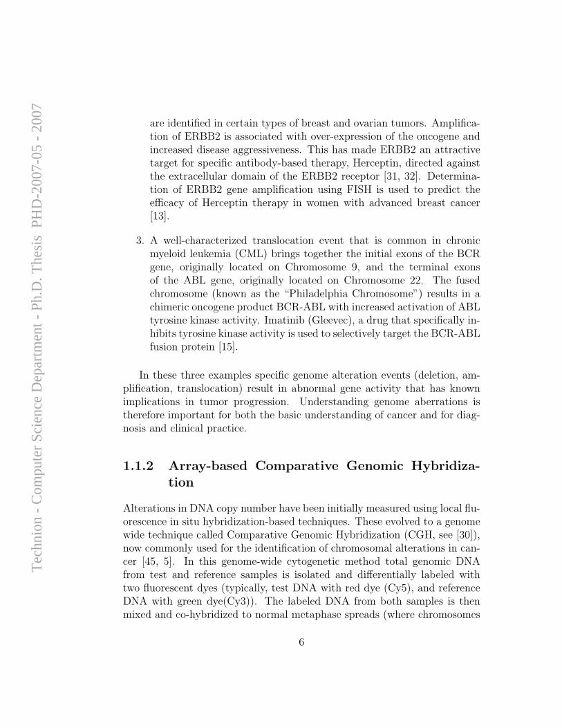
are identified in certain types of breast and ovarian tumors. Amplifica-tion of ERBB2 is associated with over-expression of the oncogene andincreased disease aggressiveness. This has made ERBB2 an attractivetarget for specific antibody-based therapy, Herceptin, directed againstthe extracellular domain of the ERBB2 receptor [31, 32]. Determina-tion of ERBB2 gene amplification using FISH is used to predict theefficacy of Herceptin therapy in women with advanced breast cancer[13].
3. A well-characterized translocation event that is common in chronicmyeloid leukemia (CML) brings together the initial exons of the BCRgene, originally located on Chromosome 9, and the terminal exonsof the ABL gene, originally located on Chromosome 22. The fusedchromosome (known as the “Philadelphia Chromosome”) results in achimeric oncogene product BCR-ABL with increased activation of ABLtyrosine kinase activity. Imatinib (Gleevec), a drug that specifically in-hibits tyrosine kinase activity is used to selectively target the BCR-ABLfusion protein [15].
In these three examples specific genome alteration events (deletion, am-plification, translocation) result in abnormal gene activity that has knownimplications in tumor progression. Understanding genome aberrations istherefore important for both the basic understanding of cancer and for diag-nosis and clinical practice.
1.1.2 Array-based Comparative Genomic Hybridiza-tion
Alterations in DNA copy number have been initially measured using local flu-orescence in situ hybridization-based techniques. These evolved to a genomewide technique called Comparative Genomic Hybridization (CGH, see [30]),now commonly used for the identification of chromosomal alterations in can-cer [45, 5]. In this genome-wide cytogenetic method total genomic DNAfrom test and reference samples is isolated and differentially labeled withtwo fluorescent dyes (typically, test DNA with red dye (Cy5), and referenceDNA with green dye(Cy3)). The labeled DNA from both samples is thenmixed and co-hybridized to normal metaphase spreads (where chromosomes
6
Tec
hnio
n -
Com
pute
r Sc
ienc
e D
epar
tmen
t - P
h.D
. The
sis
PH
D-2
007-
05 -
200
7
can be inspected visually). The relative hybridization intensity of the testand reference signals is then proportional to the relative DNA copy numbersat a given location, allowing detection of chromosomal amplifications anddeletions (see Figure 1.1c).
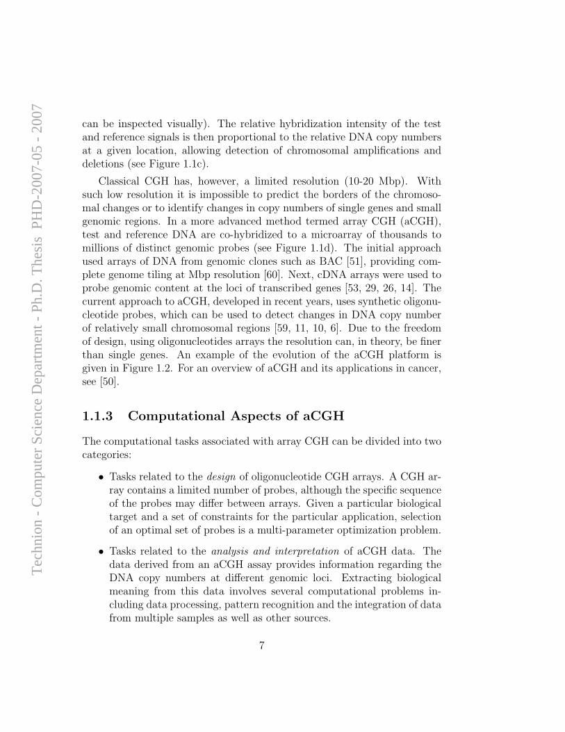
Classical CGH has, however, a limited resolution (10-20 Mbp). Withsuch low resolution it is impossible to predict the borders of the chromoso-mal changes or to identify changes in copy numbers of single genes and smallgenomic regions. In a more advanced method termed array CGH (aCGH),test and reference DNA are co-hybridized to a microarray of thousands tomillions of distinct genomic probes (see Figure 1.1d). The initial approachused arrays of DNA from genomic clones such as BAC [51], providing com-plete genome tiling at Mbp resolution [60]. Next, cDNA arrays were used toprobe genomic content at the loci of transcribed genes [53, 29, 26, 14]. Thecurrent approach to aCGH, developed in recent years, uses synthetic oligonu-cleotide probes, which can be used to detect changes in DNA copy numberof relatively small chromosomal regions [59, 11, 10, 6]. Due to the freedomof design, using oligonucleotides arrays the resolution can, in theory, be finerthan single genes. An example of the evolution of the aCGH platform isgiven in Figure 1.2. For an overview of aCGH and its applications in cancer,see [50].
1.1.3 Computational Aspects of aCGH
The computational tasks associated with array CGH can be divided into twocategories:
• Tasks related to the design of oligonucleotide CGH arrays. A CGH ar-ray contains a limited number of probes, although the specific sequenceof the probes may differ between arrays. Given a particular biologicaltarget and a set of constraints for the particular application, selectionof an optimal set of probes is a multi-parameter optimization problem.
• Tasks related to the analysis and interpretation of aCGH data. Thedata derived from an aCGH assay provides information regarding theDNA copy numbers at different genomic loci. Extracting biologicalmeaning from this data involves several computational problems in-cluding data processing, pattern recognition and the integration of datafrom multiple samples as well as other sources.
7
Tec
hnio
n -
Com
pute
r Sc
ienc
e D
epar
tmen
t - P
h.D
. The
sis
PH
D-2
007-
05 -
200
7
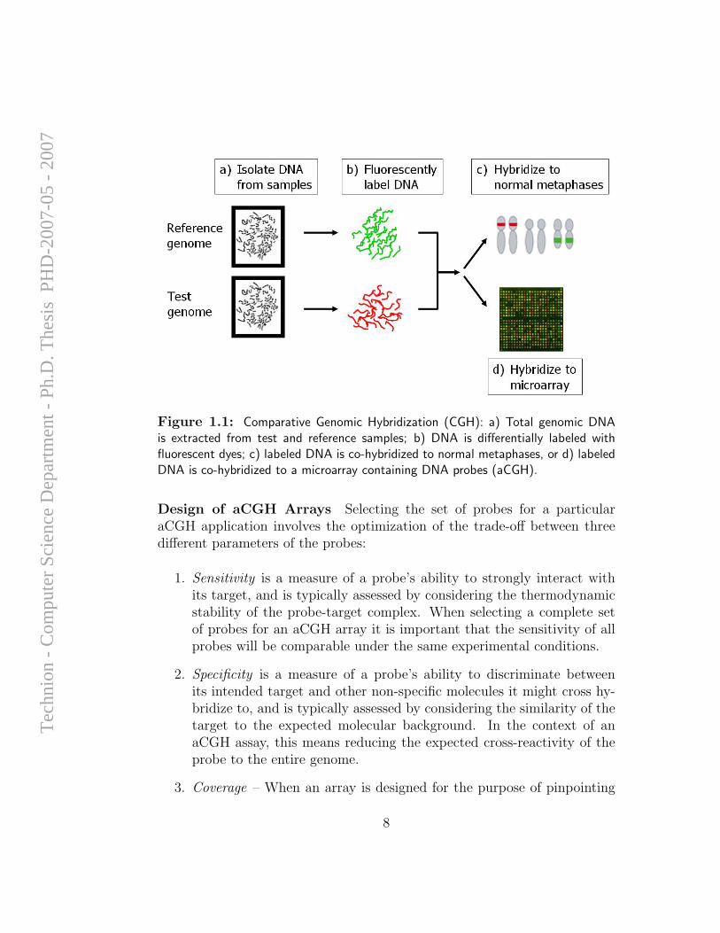
Figure 1.1: Comparative Genomic Hybridization (CGH): a) Total genomic DNAis extracted from test and reference samples; b) DNA is differentially labeled withfluorescent dyes; c) labeled DNA is co-hybridized to normal metaphases, or d) labeledDNA is co-hybridized to a microarray containing DNA probes (aCGH).
Design of aCGH Arrays Selecting the set of probes for a particularaCGH application involves the optimization of the trade-off between threedifferent parameters of the probes:
1. Sensitivity is a measure of a probe’s ability to strongly interact withits target, and is typically assessed by considering the thermodynamicstability of the probe-target complex. When selecting a complete setof probes for an aCGH array it is important that the sensitivity of allprobes will be comparable under the same experimental conditions.
2. Specificity is a measure of a probe’s ability to discriminate betweenits intended target and other non-specific molecules it might cross hy-bridize to, and is typically assessed by considering the similarity of thetarget to the expected molecular background. In the context of anaCGH assay, this means reducing the expected cross-reactivity of theprobe to the entire genome.
3. Coverage – When an array is designed for the purpose of pinpointing
8
Tec
hnio
n -
Com
pute
r Sc
ienc
e D
epar
tmen
t - P
h.D
. The
sis
PH
D-2
007-
05 -
200
7

Figure 1.2: The evolution of aCGH. Copy number changes in Chromosome 17 ofa breast cancer cell-line BT-474 measured by aCGH: a) BAC array (28 probes) [60],b) cDNA array (364 probes) [54], and c) oligonucleotide array (2,117 probes) [6].
genomic breakpoints, an important consideration in the design is tominimize the uncertainty at which the breakpoints are mapped, wher-ever they may be. Thus, probes should be somehow uniformly spaced,so as to be not “too far” from the location of any possible breakpoint.
Analysis of aCGH Data Following an aCGH experiment, the derivedDNA copy number ratios are mapped to the genomic coordinates of theprobes. Assuming that the reference sample is a normal genome, the in-creases and decreases in the measurements provide a map of the deletionsand amplifications in the genome of the test sample (see, for example, Fig-ure 1.3a).
However, biological interpretation of aCGH data is not trivial. One of the
9
Tec
hnio
n -
Com
pute
r Sc
ienc
e D
epar
tmen
t - P
h.D
. The
sis
PH
D-2
007-
05 -
200
7
central goals of DNA copy number analysis is to identify genes (and other ge-nomic elements) whose biological function is affected by genomic aberrations,and whose altered behavior has a functional effect on tumor development.To this end, computational analysis of aCGH data presents tasks of dataprocessing and interpretation, as well as tasks involving comparison of datafrom multiple experiments and of different types. The computational issuesthat will be discussed in this work are:
1. Data Centralization – Assuming that the reference is a normal genome,we typically seek to normalize aCGH signals, such that a “normal”number of copies is represented by a standard value of 0 (on a loga-rithmic scale). Since data is not guaranteed to be (and typically isn’t)normally distributed, or even symmetrically distributed, the task ofsetting the baseline is not a trivial one.
2. Aberration Calling – Given the (noisy) genomic copy number signal,the most basic analysis step is to accurately reconstruct the genomicaberration structure. Practically, we seek the set of aberrations (ge-nomic segments and their respective amplification/deletion levels) thatbest explain the observed data. For an example of aberration calls inaCGH data see Figure 1.3b.
3. Common Aberrations – Given the large degree of instability of thegenome in cancer cells, most of the genomic aberrations that are de-tected using aCGH are random events. One way of identifying aber-rations of biological importance is to determine aberrations that aresignificantly more common than would be expected at random, in agiven set of samples. The existence of common genomic aberrationssuggests that some of the random events are being selected in the evo-lutionary tumor development process.
4. Downstream Effects of Genomic Aberrations – An additional strategyfor identifying genomic aberrations with biological significance is tocorrelate the existence of specific aberrations with different downstreamelements such as expression levels of resident or distant genes, or withphenotypic data such as response to drug treatment.
10
Tec
hnio
n -
Com
pute
r Sc
ienc
e D
epar
tmen
t - P
h.D
. The
sis
PH
D-2
007-
05 -
200
7
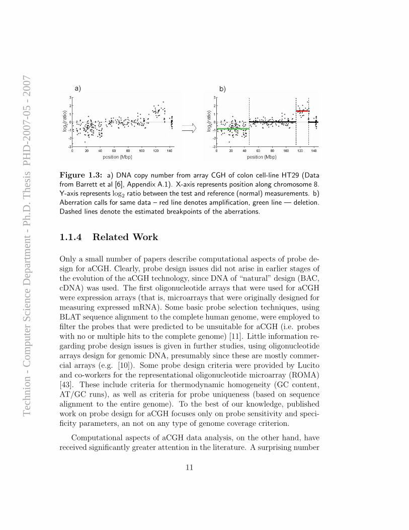
Figure 1.3: a) DNA copy number from array CGH of colon cell-line HT29 (Datafrom Barrett et al [6], Appendix A.1). X-axis represents position along chromosome 8.Y-axis represents log2 ratio between the test and reference (normal) measurements. b)Aberration calls for same data – red line denotes amplification, green line — deletion.Dashed lines denote the estimated breakpoints of the aberrations.
1.1.4 Related Work
Only a small number of papers describe computational aspects of probe de-sign for aCGH. Clearly, probe design issues did not arise in earlier stages ofthe evolution of the aCGH technology, since DNA of “natural” design (BAC,cDNA) was used. The first oligonucleotide arrays that were used for aCGHwere expression arrays (that is, microarrays that were originally designed formeasuring expressed mRNA). Some basic probe selection techniques, usingBLAT sequence alignment to the complete human genome, were employed tofilter the probes that were predicted to be unsuitable for aCGH (i.e. probeswith no or multiple hits to the complete genome) [11]. Little information re-garding probe design issues is given in further studies, using oligonucleotidearrays design for genomic DNA, presumably since these are mostly commer-cial arrays (e.g. [10]). Some probe design criteria were provided by Lucitoand co-workers for the representational oligonucleotide microarray (ROMA)[43]. These include criteria for thermodynamic homogeneity (GC content,AT/GC runs), as well as criteria for probe uniqueness (based on sequencealignment to the entire genome). To the best of our knowledge, publishedwork on probe design for aCGH focuses only on probe sensitivity and speci-ficity parameters, an not on any type of genome coverage criterion.
Computational aspects of aCGH data analysis, on the other hand, havereceived significantly greater attention in the literature. A surprising number
11
Tec
hnio
n -
Com
pute
r Sc
ienc
e D
epar
tmen
t - P
h.D
. The
sis
PH
D-2
007-
05 -
200
7
of different algorithms have been suggested for the most basic computationalproblem of aCGH data analysis, that of determining the boundaries of ampli-fication and deletion events in measurement data from a single sample. Thesuggested methods can be roughly partitioned into three general approaches:
• Smoothing algorithms – These are algorithms that do not detect theaberration boundaries directly but rather attempt to smooth the datawhile maintaining sensitivity to abrupt changes. Genomic alterationevents are then typically identified by using a threshold. Examples ofsmoothing algorithms are GLAD, based on adaptive weight smoothing[28], and a wavelet-based algorithm [27].
• Hidden Markov Model (HMM) based algorithms – These algorithmsattempt to model the underlying DNA copy numbers as hidden stateswith certain transition probabilities and emission distributions (e.g.,[21, 59]). Although this model seems reasonable HMM-based algo-rithms for aberration calling typically show relatively poor performance,presumably since more complex properties of the data are ignored (e.g.sample heterogeneity).
• Segmentation algorithms – Many of the the suggested algorithms donot detect genomic aberrations directly, but rather attempt to identifygenomic breakpoints by detecting abrupt changes in the DNA copynumber vector. The output of these algorithms is a segmentation ofthe data into segments that are relatively homogeneous, and the aber-ration calling (i.e. labeling of each segment as amplified, deleted ornormal) is done in a subsequent step. Probably the most popular ofthe segmentation methods is CBS (Circular Binary Segmentation algo-rithm [49]). Other segmentation algorithm are ChARM [47] that usesan edge detection filter, and CLAC [64], that is based on a top-downclustering approach.
Of the three approaches described above, the most successful is consideredto be the segmentation approach, since it does not assume much about thedata (unlike the HMM approach), yet gives meaningful results at the highestresolution afforded by the array (unlike the smoothing approach). A com-parison study of some of these algorithms was published by Lai et al [35]. Itshould be noted that algorithmic efficiency is not discussed in any of thesestudies, and some of the more successful algorithms are relatively slow. For
12
Tec
hnio
n -
Com
pute
r Sc
ienc
e D
epar
tmen
t - P
h.D
. The
sis
PH
D-2
007-
05 -
200
7
example, an improved version of CBS takes an order of hours to segment atypical dataset [63].
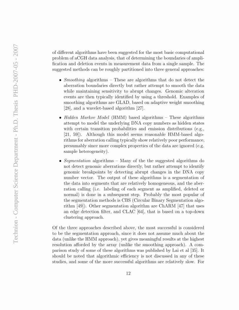
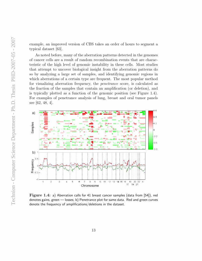
As noted before, many of the aberration patterns detected in the genomesof cancer cells are a result of random recombination events that are charac-teristic of the high level of genomic instability in these cells. Most studiesthat attempt to uncover biological insight from the aberration patterns doso by analyzing a large set of samples, and identifying genomic regions inwhich aberrations of a certain type are frequent. The most popular methodfor visualizing aberration frequency, the penetrance score, is calculated asthe fraction of the samples that contain an amplification (or deletion), andis typically plotted as a function of the genomic position (see Figure 1.4).For examples of penetrance analysis of lung, breast and oral tumor panelssee [62, 48, 4].
Figure 1.4: a) Aberration calls for 41 breast cancer samples (data from [54]), reddenotes gains, green — losses; b) Penetrance plot for same data. Red and green curvesdenote the frequency of amplifications/deletions in the dataset.
13
Tec
hnio
n -
Com
pute
r Sc
ienc
e D
epar
tmen
t - P
h.D
. The
sis
PH
D-2
007-
05 -
200
7
Although it is a useful visualization tool, the penetrance score itself doesnot convey any information regarding the statistical significance of commonaberrations. To date, little attention has been given in the literature to for-mal treatments of this task. An important exception is the work of Diskinet al [16]. The method described in this work, called STAC (SignificanceTesting for Aberrant Copy number) addresses the detection of DNA copynumber aberrations across multiple aCGH experiments by using two com-plementary statistical scores in combination with a heuristic search strategy.The significance of both statistics is assessed, and p-values are assigned toeach location in the genome by using a permutation approach. STACs searchis computationally intensive and is therefor limited to low resolution (BAC)arrays. Furthermore, it treats gains and losses as a binary signal (as doesthe penetrance score) and does not takes into account the amplitude of themeasured signal.
Perhaps the most interesting aspect of analysis of aCGH data, is thesearch for downstream effects of genomic aberrations. The basic hypothesisunderlying this research direction is that the effect of genomic aberrations onthe behavior of the cancer cell is mediated by genomic elements such as genes,or non-coding RNA, whose altered copy number causes some change in theirfunctionality. For example, an amplified gene may be over-expressed, causingthe coded protein to show an abnormally high level of activity. Most atten-tion in the literature has been given to the correlation between DNA copynumbers and expression level of protein-coding genes. Despite the existenceof some evidence to the contrary [52, 62], most studies of joint aCGH andexpression data report overwhelming correlation between changes in DNAcopy number and expression of coding genes (e.g. [54, 29, 36, 2]). A dif-ferent view of downstream effects of genomic aberrations may be unveiledby examining the correlations of changes in DNA copy number with phe-notypic data, such as drug response profiles. Two recent studies using theNCI-60 cell line panel showed that significant correlation of this type doesexist for selected genes [22, 12]. In the first of these two studies Garraway andco-workers identified and validated the implication of an amplification of aspecific transcription factor (MITF) on the sensitivity of melanoma cell-linesto specific chemotherapeutic agents, thus implying that direct targeting ofthis amplified gene may offer a potential therapeutic approach to melanoma.
14
Tec
hnio
n -
Com
pute
r Sc
ienc
e D
epar
tmen
t - P
h.D
. The
sis
PH
D-2
007-
05 -
200
7
1.2 Overview
In this thesis, I present the work I have done, together with different col-laborators, on the development of computational tools and methods for thedesign of aCGH arrays and the analysis of DNA copy number data. Most ofthe work has been published in several papers that appear in an appendix ofthis thesis (Appendix A).
The contribution of the work contained in these papers is summarizedin the Results Chapter. Methods for design of CGH arrays are presentedin Section 2.1 and methods for aCGH analysis are presented in Section 2.2,including recent results whose publication is in preparation (Sections 2.2.4-2.2.5). Some additional related results are presented in Section 2.3. Theimplications of our work are presented in the Discussion Chapter, as well asfuture directions in which this work may be continued.
15
Tec
hnio
n -
Com
pute
r Sc
ienc
e D
epar
tmen
t - P
h.D
. The
sis
PH
D-2
007-
05 -
200
7

16
Tec
hnio
n -
Com
pute
r Sc
ienc
e D
epar
tmen
t - P
h.D
. The
sis
PH
D-2
007-
05 -
200
7
Chapter 2
Results
2.1 Design of CGH Arrays
The progression of aCGH to the oligonucleotide microarray platform openeda large variety of possibilities for biological applications that were infeasiblewith previous platforms. If probe selection in BAC and cDNA was constrictedto existing BAC and cDNA libraries, oligonucleotide probes can be designedfor any desired genomic target, as well as for hypothetical targets (such asrearranged genomic sequences).
Design of the first aCGH specific oligonucleotide microarrays, in collabo-ration with the Bio-Medical Assays Group (BMAG) at Agilent Laboratories,was targeted at the application of measuring DNA copy numbers of theentire human genome. The computational problems associated with this ap-plication were mostly focused on determining parameters for prediction andassessment of probe performance and implementing efficient tools for opti-mal selection of high-performing probes from a large (order of 108) set ofcandidate probes.
As oligo-based aCGH matured, applications requiring custom High-DefinitionCGH arrays (HD-CGH) imposed additional optimization constraints on thearray design problem. HD-CGH arrays are typically intended to measurechanges in DNA copy number of specific genomic regions, in extremely highresolution. Methods for optimizing probe coverage, in addition to probeperformance, are required in this setting.
17
Tec
hnio
n -
Com
pute
r Sc
ienc
e D
epar
tmen
t - P
h.D
. The
sis
PH
D-2
007-
05 -
200
7
2.1.1 Optimization of Probe Performance
The advancement of a robust and flexible oligonucleotide aCGH platform, incollaboration with the Bio-Medical Assays Group at Agilent Laboratories, isdescribed in the following paper [6]. Here I summarize the computationalaspects of this, and related, work:
• M.T. Barrett, A. Scheffer, A. Ben-Dor, N. Sampas, D. Lipson, R. Kin-caid, P. Tsang, B. Curry, K. Baird, P.S. Meltzer, Z. Yakhini, L. Bruhn,and S. Laderman. “Comparative Genomic Hybridization us-ing Oligonucleotide Microarrays and Total Genomic DNA”.PNAS, Vol. 101, No. 51, 21 December 2004, pp. 17765-17770. (Ap-pendix A.1)
The first attempt to measure copy numbers of genomic DNA using anoligonucleotide microarray was performed on an expression array (human1A microarray, Agilent Technologies) containing probes for 17,086 uniquegenes. This set of probes was filtered by comparing all probe sequences to thesequence of the entire human genome (UCSC build hg12, June 2002 [33]). 755probes were removed since they were not contiguous in the genome, probablydue to crossing of exon-intron boundaries or errors in transcript sequences.5,175 additional probes that, although unique in the transcriptome, gavemore than one hit in the genome were also removed from the analysis.
To begin exploring the freedom of design that oligo arrays allow, wecreated arrays that included 21,253 probes representing unique genomic se-quences that span chromosomes 16, 17, 18 and X at average spacings of16, 10.5, 23 and 31 Kbp, respectively. These probes, in contrast to theprobes on the expression arrays that are restricted to the 3’ regions of ex-pressed sequences, represent unique genomic sequences, include coding andnon-coding sequences, and have a narrower range of Tm (melting tempera-ture) values. The initial assessment of the performance of the array was doneby hybridization to cell lines with variable copy numbers of the X chromo-some (1-5 copies), compared to 2X DNA as reference. Figure 2.1 shows acomparison of the median log-ratios for the X-chromosome probes from thesehybridizations on the expression array (373 probes) and the CGH array (4,878probes). Notably, the median ratios for the measured values on the CGH ar-rays are in closest agreement with the expected values (−1, 0, log2
32, 1, log2
52).
18
Tec
hnio
n -
Com
pute
r Sc
ienc
e D
epar
tmen
t - P
h.D
. The
sis
PH
D-2
007-
05 -
200
7
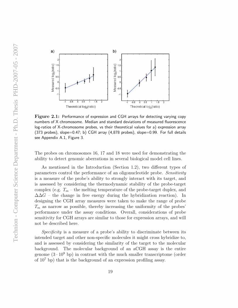
Figure 2.1: Performance of expression and CGH arrays for detecting varying copynumbers of X chromosome. Median and standard deviations of measured fluorescencelog-ratios of X-chromosome probes, vs their theoretical values for a) expression array(373 probes), slope=0.47; b) CGH array (4,878 probes), slope=0.99. For full detailssee Appendix A.1, Figure 3.
The probes on chromosomes 16, 17 and 18 were used for demonstrating theability to detect genomic aberrations in several biological model cell lines.
As mentioned in the Introduction (Section 1.2), two different types ofparameters control the performance of an oligonucleotide probe. Sensitivityis a measure of the probe’s ability to strongly interact with its target, andis assessed by considering the thermodynamic stability of the probe-targetcomplex (e.g. Tm – the melting temperature of the probe-target duplex, and∆∆G – the change in free energy during the hybridization reaction). Indesigning the CGH array measures were taken to make the range of probeTm as narrow as possible, thereby increasing the uniformity of the probes’performance under the assay conditions. Overall, considerations of probesensitivity for CGH arrays are similar to those for expression arrays, and willnot be described here.
Specificity is a measure of a probe’s ability to discriminate between itsintended target and other non-specific molecules it might cross hybridize to,and is assessed by considering the similarity of the target to the molecularbackground. The molecular background of an aCGH assay is the entiregenome (3 · 109 bp) in contrast with the much smaller transcriptome (orderof 107 bp) that is the background of an expression profiling assay.
19
Tec
hnio
n -
Com
pute
r Sc
ienc
e D
epar
tmen
t - P
h.D
. The
sis
PH
D-2
007-
05 -
200
7
Homology to the human genome background was assessed using the Probe-Spec application, that was developed by us for probe specificity analysis forexpression microarrays [41]. Basically, the application performs a index-based search similar to BLAST [3] and reports all homologous subsequencesof the background sequence that are within a pre-specified Hamming dis-tance, or other distance measures, from the query (target) sequence. Here,we modified the application to account for the much larger human genomebackground. Since the entire genome can not be processed (or even main-tained in memory) at one time, the application was broken down into twoparts – an indexing application and a scoring application. The indexing ap-plication partitions the background into multiple exclusive subsequences thatare indexed separately, while the scoring application scores the given probesequences by sequentially loading and searching each of the index files.
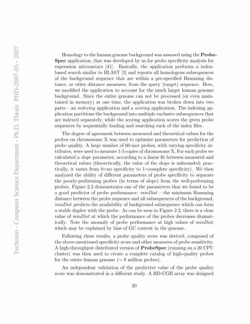
The degree of agreement between measured and theoretical values for theprobes on chromosome X was used to optimize parameters for prediction ofprobe quality. A large number of 60-mer probes, with varying specificity at-tributes, were used to measure 1-5 copies of chromosome X. For each probe wecalculated a slope parameter, according to a linear fit between measured andtheoretical values (theoretically, the value of the slope is unbounded; prac-tically, it varies from 0=no specificity to 1=complete specificity). We thenanalyzed the ability of different parameters of probe specificity to separatethe poorly-performing probes (in terms of slope) from the well-performingprobes. Figure 2.2 demonstrates one of the parameters that we found to bea good predictor of probe performance: minDist – the minimum Hammingdistance between the probe sequence and all subsequences of the background.minDist predicts the availability of background subsequence which can forma stable duplex with the probe. As can be seen in Figure 2.2, there is a clearvalue of minDist at which the performance of the probes decreases dramat-ically. Note the anomaly of probe performance at high values of minDist,which may be explained by bias of GC content in the genome.
Following these results, a probe quality score was derived, composed ofthe above-mentioned specificity score and other measures of probe sensitivity.A high-throughput distributed version of ProbeSpec (running on a 20 CPUcluster) was then used to create a complete catalog of high-quality probesfor the entire human genome (∼ 8 million probes).
An independent validation of the predictive value of the probe qualityscore was demonstrated in a different study. A HD-CGH array was designed
20
Tec
hnio
n -
Com
pute
r Sc
ienc
e D
epar
tmen
t - P
h.D
. The
sis
PH
D-2
007-
05 -
200
7
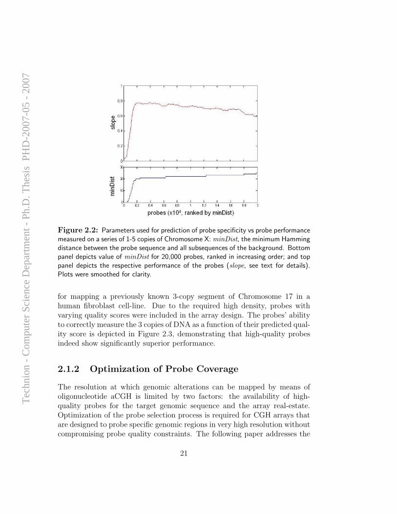
Figure 2.2: Parameters used for prediction of probe specificity vs probe performancemeasured on a series of 1-5 copies of Chromosome X: minDist, the minimum Hammingdistance between the probe sequence and all subsequences of the background. Bottompanel depicts value of minDist for 20,000 probes, ranked in increasing order; and toppanel depicts the respective performance of the probes (slope, see text for details).Plots were smoothed for clarity.
for mapping a previously known 3-copy segment of Chromosome 17 in ahuman fibroblast cell-line. Due to the required high density, probes withvarying quality scores were included in the array design. The probes’ abilityto correctly measure the 3 copies of DNA as a function of their predicted qual-ity score is depicted in Figure 2.3, demonstrating that high-quality probesindeed show significantly superior performance.
2.1.2 Optimization of Probe Coverage
The resolution at which genomic alterations can be mapped by means ofoligonucleotide aCGH is limited by two factors: the availability of high-quality probes for the target genomic sequence and the array real-estate.Optimization of the probe selection process is required for CGH arrays thatare designed to probe specific genomic regions in very high resolution withoutcompromising probe quality constraints. The following paper addresses the
21
Tec
hnio
n -
Com
pute
r Sc
ienc
e D
epar
tmen
t - P
h.D
. The
sis
PH
D-2
007-
05 -
200
7
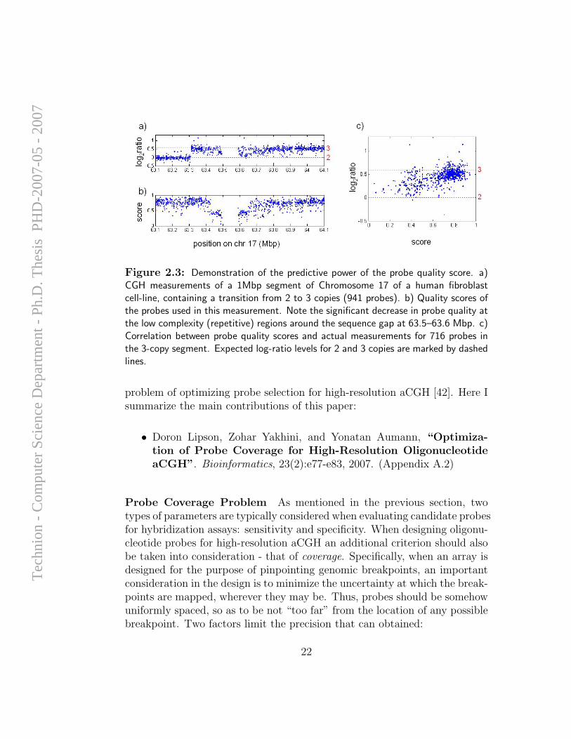
Figure 2.3: Demonstration of the predictive power of the probe quality score. a)CGH measurements of a 1Mbp segment of Chromosome 17 of a human fibroblastcell-line, containing a transition from 2 to 3 copies (941 probes). b) Quality scores ofthe probes used in this measurement. Note the significant decrease in probe quality atthe low complexity (repetitive) regions around the sequence gap at 63.5–63.6 Mbp. c)Correlation between probe quality scores and actual measurements for 716 probes inthe 3-copy segment. Expected log-ratio levels for 2 and 3 copies are marked by dashedlines.
problem of optimizing probe selection for high-resolution aCGH [42]. Here Isummarize the main contributions of this paper:
• Doron Lipson, Zohar Yakhini, and Yonatan Aumann, “Optimiza-tion of Probe Coverage for High-Resolution OligonucleotideaCGH”. Bioinformatics, 23(2):e77-e83, 2007. (Appendix A.2)
Probe Coverage Problem As mentioned in the previous section, twotypes of parameters are typically considered when evaluating candidate probesfor hybridization assays: sensitivity and specificity. When designing oligonu-cleotide probes for high-resolution aCGH an additional criterion should alsobe taken into consideration - that of coverage. Specifically, when an array isdesigned for the purpose of pinpointing genomic breakpoints, an importantconsideration in the design is to minimize the uncertainty at which the break-points are mapped, wherever they may be. Thus, probes should be somehowuniformly spaced, so as to be not “too far” from the location of any possiblebreakpoint. Two factors limit the precision that can obtained:
22
Tec
hnio
n -
Com
pute
r Sc
ienc
e D
epar
tmen
t - P
h.D
. The
sis
PH
D-2
007-
05 -
200
7
• With a limited array capacity, probes cannot be placed at each genomiclocation. Rather, they must be spread across the region of interest. Inthis case, the localization of a genomic event can only be determined bythe pair of flanking probes. We shall seek that for all genomic locations,the gap between this pair of probes is as small as possible.
• Some genomic regions do not contain any candidate probes, or onlyprobes of poor quality. In such cases, large gaps between probes areinevitable. Any breakpoint occurring within these gaps can only pos-sibly be localized to within the pair of candidate probes bordering thegap.
Thus, we seek to choose a set of probes that is uniformly close to all genomiclocations – whenever possible, and as close as possible to the points withinthe large gaps. The following definition captures this intuition:
Definition 2.1.1 (Whenever Possible (WP) ε-cover) Given a genomicregion G, a set of candidate probes P and a parameter ε, a subset C =(c1, . . . , ck) ⊆ P is a whenever possible ε-cover of G with respect to P if forany genomic location x ∈ G, the following holds. Let ci and ci+1 be the twoselected probes closest to x from the left and from the right, respectively (ifx < c1 then c0 is set to be the left-end of G, and for x > ck, ck+1 is theright-end of G). Then, one of the following holds:
1. ci+1 − ci ≤ ε (i.e. the flanking selected probes are within ε distance ofeach other), or
2. there is no candidate probe between ci and ci+1.
For such a cover C, we say that the resolution of C is ε.
Assume that we are given as set of probes P = (p1, . . . , pn) identified bytheir genomic location: P ⊂ N. Let q : P → R+ be the quality functionassociating a quality score with each probe (local measures of quality arealso applicable). Given a fixed number of probes in the array, the problemof designing an aCGH array is therefore a bicriteria optimization problem:Select a subset of probes that are (i) of high quality (ii) with high resolution.A standard approach to such bicriteria problems is to optimize one criterion,given a constraint on the other. In our case, this gives rise to the followingoptimization problem:
23
Tec
hnio
n -
Com
pute
r Sc
ienc
e D
epar
tmen
t - P
h.D
. The
sis
PH
D-2
007-
05 -
200
7
Problem 2.1.2 (Probe Selection – Resolution Optimization) Given aninteger k, genomic region G and quality threshold τ , find the minimal possibleresolution ε∗ and a probe subset C ⊂ P such that:
1. |C| = k,
2. C contains only τ -good probes,
3. C is a WP ε∗-cover of G with respect to the τ -good probes.
UniProbe Algorithm Given a quality threshold τ we can filter P to in-clude only τ -good probes. In order to solve the resolution optimization prob-lem, we first consider the reverse optimization problem:
Problem 2.1.3 Given a genomic region G and a fixed value of ε, find a WPε-cover C for G of minimal size.
It is easy to show that a greedy algorithm solves this problem in linear time(see Appendix A.2, Algorithm 1).
In the probe selection problem, we are given a number k of probes andseek to optimize the resolution. We do so by performing a binary searchon the resolutions, using the greedy algorithm as the decision criteria. Theprocedure performs a binary search for the optimal ε within the range [1, |G|].Clearly, the optimal ε is a distance between some two probes pi, pj ∈ P(otherwise, ε could be reduced to the closest distance). There are O(n2)such pairwise distances. Thus a balanced binary search could pinpoint theoptimal value in O(log n) recursive calls. However, these O(n2) pairwisedistances are not provided to us explicitly, and enumerating them all wouldtake O(n2) steps by itself. Thus, we seek to somehow perform a balancedbinary search on this O(n2)-sized space without explicitly enumerating it.Interestingly, this can be done in O(n log n) time. The key element is to finda good split value (pivot) in linear time. We provide a randomized procedureto find such a split value efficiently (see Appendix A.2, Algorithm 3). Thealgorithm is implemented in an application called UniProbe.
Application We demonstrate the application of UniProbe on a typicalscenario of high-resolution probe design. Assume we are searching for a
24
Tec
hnio
n -
Com
pute
r Sc
ienc
e D
epar
tmen
t - P
h.D
. The
sis
PH
D-2
007-
05 -
200
7
genomic breakpoint at the 6 Mbp p-terminus of chromosome 10. Given a setof 82,500 quality-scored candidate probes taken from a probe database, wewould like to select 3,000 oligonucleotide probes that offer the best guaranteedresolution of detecting breakpoints. In theory, placing the probes at equalspacing would provide a guaranteed 2Kbp resolution, in the sense that thegenomic distance between each pair of consecutive probes would be 2Kbp.However, achieving this theoretical resolution is impossible due to unclosedgaps in the genomic sequence and regions with low quality probes.
We compare the set of probes selected by UniProbe to two different naivemethods for uniformly-spaced probe selection. The first method (Qual) se-lects probes on the basis of their quality alone, assuming that randomnessin the positions of the superior probes will lead to some degree of unifor-mity in their coverage. The second naive method (Bin) is based on binning:The total genomic segment is divided into 3,000 equally-sized bins, and thehighest-quality probe in each bin is selected. Note that no probes can beselected from empty bins, reducing the total number of selected probes tobelow 3,000.
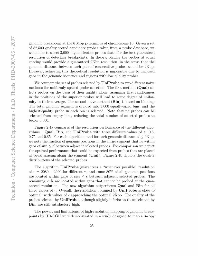
Figure 2.4a compares of the resolution performance of the different algo-rithms – Qual, Bin, and UniProbe with three different values of τ : 0.5,0.75 and 0.85. For each algorithm, and for each genomic distance d ≤ 6Kbp,we note the fraction of genomic positions in the entire segment that lie withingaps of size ≤ d between adjacent selected probes. For comparison we depictthe optimal performance that could be expected from probes that are placedat equal spacing along the segment (Unif). Figure 2.4b depicts the qualitydistributions of the selected probes.
The algorithm UniProbe guarantees a “whenever possible” resolutionof ε = 2080 − 2260 for different τ , and some 80% of all genomic positionsare located within gaps of size ≤ ε between adjacent selected probes. Theremaining 20% are located within gaps that cannot be probed at the guar-anteed resolution. The new algorithm outperforms Qual and Bin for allthree values of τ . Overall, the resolution obtained by UniProbe is close tooptimal, with values of ε approaching the optimal 2Kbp. The quality of theprobes selected by UniProbe, although slightly inferior to those selected byBin, are still satisfactory high.
The power, and limitations, of high-resolution mapping of genomic break-points by HD-CGH were demonstrated in a study designed to map a 3-copy
25
Tec
hnio
n -
Com
pute
r Sc
ienc
e D
epar
tmen
t - P
h.D
. The
sis
PH
D-2
007-
05 -
200
7
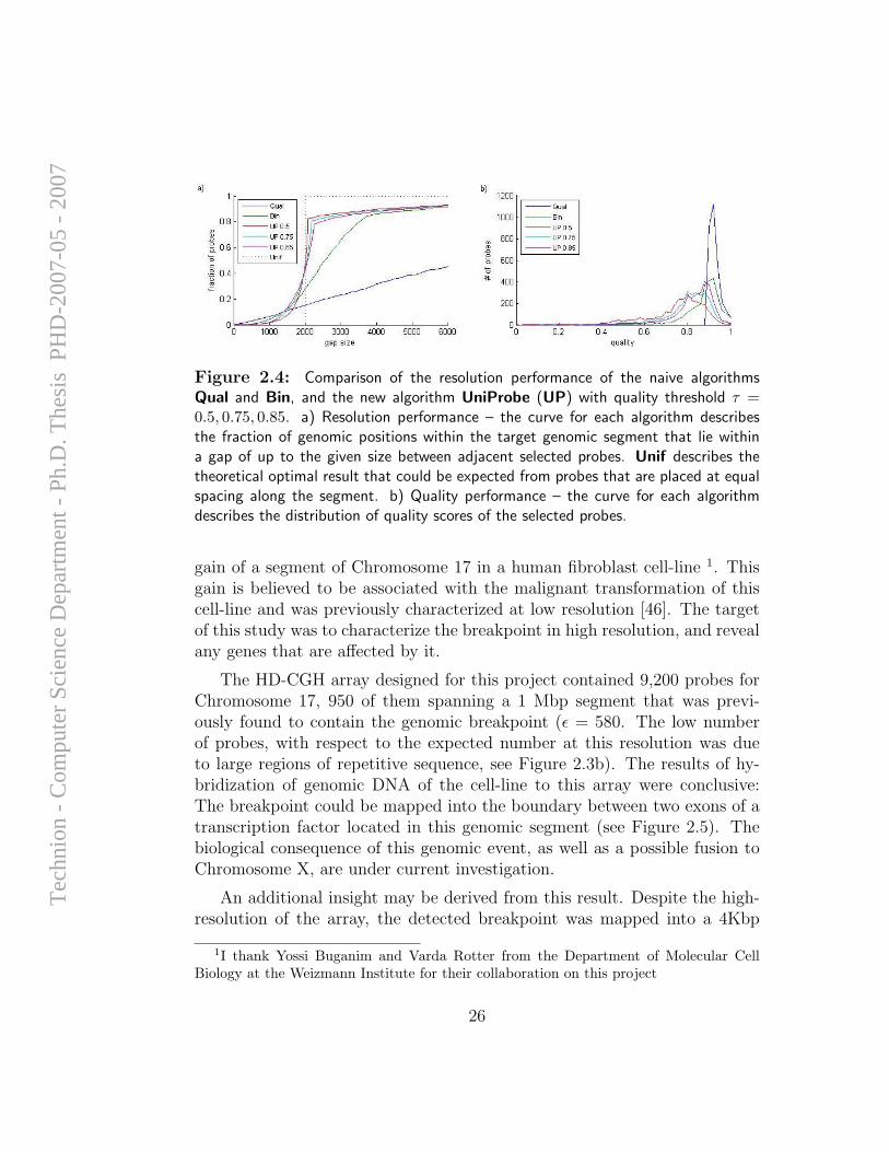
Figure 2.4: Comparison of the resolution performance of the naive algorithmsQual and Bin, and the new algorithm UniProbe (UP) with quality threshold τ =0.5, 0.75, 0.85. a) Resolution performance – the curve for each algorithm describesthe fraction of genomic positions within the target genomic segment that lie withina gap of up to the given size between adjacent selected probes. Unif describes thetheoretical optimal result that could be expected from probes that are placed at equalspacing along the segment. b) Quality performance – the curve for each algorithmdescribes the distribution of quality scores of the selected probes.
gain of a segment of Chromosome 17 in a human fibroblast cell-line 1. Thisgain is believed to be associated with the malignant transformation of thiscell-line and was previously characterized at low resolution [46]. The targetof this study was to characterize the breakpoint in high resolution, and revealany genes that are affected by it.
The HD-CGH array designed for this project contained 9,200 probes forChromosome 17, 950 of them spanning a 1 Mbp segment that was previ-ously found to contain the genomic breakpoint (ε = 580. The low numberof probes, with respect to the expected number at this resolution was dueto large regions of repetitive sequence, see Figure 2.3b). The results of hy-bridization of genomic DNA of the cell-line to this array were conclusive:The breakpoint could be mapped into the boundary between two exons of atranscription factor located in this genomic segment (see Figure 2.5). Thebiological consequence of this genomic event, as well as a possible fusion toChromosome X, are under current investigation.
An additional insight may be derived from this result. Despite the high-resolution of the array, the detected breakpoint was mapped into a 4Kbp
1I thank Yossi Buganim and Varda Rotter from the Department of Molecular CellBiology at the Weizmann Institute for their collaboration on this project
26
Tec
hnio
n -
Com
pute
r Sc
ienc
e D
epar
tmen
t - P
h.D
. The
sis
PH
D-2
007-
05 -
200
7
Figure 2.5: HD-CGH analysis of genomic breakpoint in 17q: a) CGH measurementsof 1 Mbp segment of 17q in human fibroblast cell-line (2 and 3 copies denoted bydashed lines). b) Alignment of detected breakpoint to UCSC genome browser [33]maps breakpoint onto intronic sequence of a transcription factor.
gap between adjacent probes. No decent-quality probes could be obtained inthis gap, making this result unavoidable. The fact that the breakpoint of thegenomic event occurs at this low-complexity repetitive sequence is probablynot a coincidence and underlines the fact that genomic breakpoints havean inclination to take place at repetitive sequences. Therefore, our abilityto map such breakpoints at ultra-high resolution using any sequence-basedtechnology may be inherently limited.
27
Tec
hnio
n -
Com
pute
r Sc
ienc
e D
epar
tmen
t - P
h.D
. The
sis
PH
D-2
007-
05 -
200
7
2.2 Analysis of aCGH Data
The output of an aCGH assay is vector of DNA copy number values thatcan be mapped to the genomic coordinates of the probes (e.g., Figure 1.3a).Biological interpretation of this vector is performed at two levels. First is theinterpretation of the genomic aberrations at a single-sample sample. Thisinvolves normalization of the data, and identifying genomic segments thatcontain a deletion or amplification. The second level includes analyses ofpanels of multiple samples, attempting to discover biologically-meaningfulpatterns that emerge from the background of seemingly random genomicaberration events.
Here I will describe our approach to normalization and aberration callingin DNA copy number data from a single sample, based on a highly-efficientalgorithm called Stepgram. Stepgram is now used as a basic data processingtool in several aCGH analysis packages, including the commercial CGH-Analytics [1]. I will also describe some of our work on biological interpretationof DNA copy number changes, based on a statistical framework for analysis ofcommon aberrations, and integration of aCGH, expression, and drug responseprofile data on the NCI-60 panel of cell-lines.
In a recent study, we used CGH arrays to measure the time-course ofreplication of genomic DNA in mouse cells. Despite the drastically differentbiological nature of this process we used the tools developed for analysis ofgenomic aberrations to characterize the different segments of the genome thatare replicated at various stages of the S-phase of the cell-cycle. The resultsobtained in this study demonstrate the applicability of these tools to a widerange of applications.
2.2.1 Aberration Calling
The first step in analyzing DNA copy number data from aCGH arrays con-sists of identifying aberrant (amplified or deleted) regions in each individualsample. Our approach to this problem, including several efficient algorithmsfor data analysis, is described in the following paper [37]. Here I summarizethe main contributions of this paper:
• Doron Lipson, Yonatan Aumann, Amir Ben-Dor, Nathan Linial, andZohar Yakhini. “Efficient Calculation of Interval Scores for
28
Tec
hnio
n -
Com
pute
r Sc
ienc
e D
epar
tmen
t - P
h.D
. The
sis
PH
D-2
007-
05 -
200
7

DNA Copy Number Data Analysis”. Proceedings of RECOMB’05, LNCS 3500, p. 83, Springer-Verlag, 2005. Also in Journal of Com-putational Biology, Vol. 13, No. 2: 215-228, 2006. (Appendix A.3)
As described in the Introduction (Section 1.1.4) current literature on an-alyzing DNA copy number data describes several approaches to the task ofcalling aberrations, the most popular of which are based on segmenting thedata into relatively homogeneous segments based on identification of abruptchanges in the distribution of the data points (e.g. [64, 49]). Our approachdiffers from others by the fact that we search directly for genomic inter-vals with consistent high or low signals which significantly deviate from thebaseline (corresponding to a normal genome), rather than searching for thebreakpoints.
The Maximum Scoring Interval Problem Let V = (v1, · · · , vn) de-note a vector of DNA copy number data for a genomic segment (e.g., a chro-mosome), where vi denotes the (normalized) data for the i-th probe alongthe segment. The underlying model of chromosomal instabilities suggeststhat amplification and deletion events typically span several probes alongthe chromosome. Therefore, if the target chromosome contains amplificationor deletion events then we expect to see many consecutive positive entriesin V (amplification), or many consecutive negative entries (deletion). Onthe other hand, if the target chromosome is normal (no aberration), we ex-pect no localized effects. Intuitively, we look for intervals (sets of consecutiveprobes) where signal sums are significantly larger or significantly smaller thanexpected at random. To formalize this intuition we assume (null model) thatthere is no aberration present in the target DNA, and therefore the variationin V represents only the noise of the measurement.
Assuming that the measurement noise along the chromosome is indepen-dent for distinct probes and normally distributed, let µ and σ denote themean and standard deviation of the normal genomic data (typically, afternormalization µ = 0). Given an interval I spanning |I| probes, let
ϕ(I) =∑i∈I
(vi − µ)
σ√|I|
.
Under the null model, ϕ(I) has a Normal(0, 1) distribution, for any I.Thus, We can use ϕ(I) (which does not depend on probe density) to assess
29
Tec
hnio
n -
Com
pute
r Sc
ienc
e D
epar
tmen
t - P
h.D
. The
sis
PH
D-2
007-
05 -
200
7
the statistical significance of values in I using a large deviation bound [19].Given a vector V , we therefore seek all intervals I with |ϕ(I)| exceeding acertain threshold. Setting the threshold to avoid false positives we reportall these intervals as putative aberrations. This formulation gives rise to thefollowing optimization problem:
Problem 2.2.1 (Maximum Scoring Interval) Given a vector V , find theinterval I ⊆ [1, n] that maximizes the score ϕ(I).
Clearly, finding the interval with maximal score can be done by exhaustivesearch, checking all possible intervals. However, even for a single sample casethis would take O(n2) steps, which rapidly becomes time consuming, as thenumber of measured genomic loci grows to tens of thousands. Moreover,even for n ≈ 104 O(n2) does not allow for interactive data analysis, which iscalled for by practitioners.
LookAhead Algorithm We describe two algorithms for finding the inter-val with maximal score in subquadratic time. The first, called LookAhead,is a branch-and-bound approach. The algorithm operates by considering allpossible interval start-points, in sequence. For each start-point i, we checkthe intervals with endpoints in increasing distance from i. The basic idea isto try and not consider all possible endpoints, but rather to skip some thatwill clearly not provide the optimum. Assume that we are given two param-eters t and m, where t is a lower bound on the optimal score (t ≤ maxI ϕ(I))and m is an upper bound on the value of any single element (m ≥ maxi vi).Assume that we have just considered an interval of length k: I = [i, i+k−1]with σ =
∑i∈I vi, and ϕ(I) = σ√
k. After checking the interval I, an exhaus-
tive algorithm would continue to the next endpoint, and check the intervalI1 = [i, i+k]. However, this might not always be necessary. If σ is sufficientlysmall and k is sufficiently large then I1 may stand no chance of obtainingϕ(I1) > t. Thus, using these parameters we can determine the first valueof x for which ϕ(Ix) has a chance of surpassing t, and skip the next (x− 1)intervals.
The improvement in efficiency depends on the actual number of endpointsthat are skipped. This number, in turn, depends on the tightness of the twobounds t and m. Various considerations and pre-processing procedures canbe used to achieve improved bounds, where the most efficient variation yieldsa practical O(n1.5) running time (see Appendix A.3, Algorithm 2).
30
Tec
hnio
n -
Com
pute
r Sc
ienc
e D
epar
tmen
t - P
h.D
. The
sis
PH
D-2
007-
05 -
200
7
Geometric Family Algorithm A second algorithm, is based on a lineartime approximation scheme. We define a family I of intervals of increasinglengths, the geometric family, as follows. For integral j, let kj = (1+ ε)j and∆j = εkj. For j = 0, . . . , log(1+ε) n, let
I(j) =
{[i∆j, i∆j + kj − 1] : 0 ≤ i ≤ n− kj
∆j
}In words, I(j) consists of intervals of size kj evenly spaced ∆j apart. Set
I = ∪log(1+ε) n
j=0 I(j). The approximation algorithm, named GFA (for Geomet-ric Family Approximation), simply computes scores for all J ∈ I and outputsthe highest scoring one (see Appendix A.3, Algorithm 1). We prove that, forε ≤ 1/5, this algorithm provides an α(ε) = (1 −
√2ε(2 + ε))−1 approxima-
tion to the maximal score. Note that α(ε) → 1 as ε → 0. Hence, the aboveconstitutes an approximation scheme. The complexity of the algorithm isdetermined by the number of intervals in I. For each j, the intervals of Ij
are ∆j apart. Thus, |Ij| ≤ n∆j
= nε(1+ε)j . Hence, the total complexity of the
algorithm is:
|I| ≤log(1+ε) n∑
j=0
n
ε(1 + ε)−j ≤ n
ε
∞∑j=0
(1 + ε)−j = ε−2n = O(nε−2)
Let M be the maximum score of the intervals in I. To find the maximalscore of all intervals, we concentrate only on intervals J ∈ I with ϕ(J) ≥M/α. For each interval J we define the cover zone of J to be those intervals Ifor which J is the leftmost largest interval. We then search these cover zonesusing LookAhead for the true optimum. Although the worst-case runningtime of GFA is O(n2), its practical running time is linear.
Applications Figure 2.6 depicts results of benchmarking the Exhaustive,LookAhead and GFA algorithms on synthetic data as well as data frombiological origin. Although GFA appears to show the best asymptotic per-formance (linear), for current values of n both LookAhead and GFA performequally well, outperforming the exhaustive approach significantly.
Above, we presented algorithms for finding the single highest scoring in-terval. Practically, we are interested in finding all intervals with scores above
31
Tec
hnio
n -
Com
pute
r Sc
ienc
e D
epar
tmen
t - P
h.D
. The
sis
PH
D-2
007-
05 -
200
7
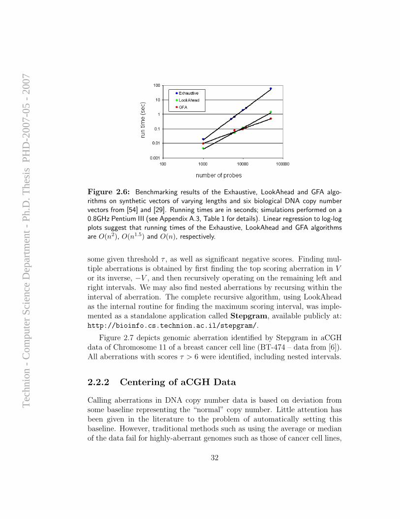
Figure 2.6: Benchmarking results of the Exhaustive, LookAhead and GFA algo-rithms on synthetic vectors of varying lengths and six biological DNA copy numbervectors from [54] and [29]. Running times are in seconds; simulations performed on a0.8GHz Pentium III (see Appendix A.3, Table 1 for details). Linear regression to log-logplots suggest that running times of the Exhaustive, LookAhead and GFA algorithmsare O(n2), O(n1.5) and O(n), respectively.
some given threshold τ , as well as significant negative scores. Finding mul-tiple aberrations is obtained by first finding the top scoring aberration in Vor its inverse, −V , and then recursively operating on the remaining left andright intervals. We may also find nested aberrations by recursing within theinterval of aberration. The complete recursive algorithm, using LookAheadas the internal routine for finding the maximum scoring interval, was imple-mented as a standalone application called Stepgram, available publicly at:http://bioinfo.cs.technion.ac.il/stepgram/.
Figure 2.7 depicts genomic aberration identified by Stepgram in aCGHdata of Chromosome 11 of a breast cancer cell line (BT-474 – data from [6]).All aberrations with scores τ > 6 were identified, including nested intervals.
2.2.2 Centering of aCGH Data
Calling aberrations in DNA copy number data is based on deviation fromsome baseline representing the “normal” copy number. Little attention hasbeen given in the literature to the problem of automatically setting thisbaseline. However, traditional methods such as using the average or medianof the data fail for highly-aberrant genomes such as those of cancer cell lines,
32
Tec
hnio
n -
Com
pute
r Sc
ienc
e D
epar
tmen
t - P
h.D
. The
sis
PH
D-2
007-
05 -
200
7

Figure 2.7: Significant alterations in breast cancer cell line BT-474, Chromosome11 (2,072 probes, data from [6]), identified by Stepgram with threshold τ = 4. a)Raw aCGH data; b) Identified aberrations: Red intervals denote amplifications, greenintervals — deletions.
due abnormality of the distribution of the measurements. Our approach tothe problem of aCGH data centering is described in the following paper [39].Here I summarize the main contributions of this paper:
• Doron Lipson, Amir Ben-Dor, and Zohar Yakhini. “Determining theCenter of array-CGH Data”. In preparation. (Appendix A.4)
The basis for assigning a statistical aberration score to an interval involvesthe assumption of a zero value for the data – the mean around which weexpect the data to be distributed when no aberration occurred. Currently,aCGH data fluorescence ratios are typically normalized for each array bysetting the average log fluorescence ratio for all array elements to zero. Forillustration, consider a male vs female aCGH assay. As all probes residing onchromosome X are expected to yield a non-zero log fluorescence ratio and allother probes are expected to yield signals centered around zero we don’t, infact, expect the normalization above to yield a value that represents the realcenter of the diploid part of the sample. In this case, it is easy to overcome
33
Tec
hnio
n -
Com
pute
r Sc
ienc
e D
epar
tmen
t - P
h.D
. The
sis
PH
D-2
007-
05 -
200
7
the problem by excluding the X chromosome from the centralization process,but in most cases the aberrant regions of the genome are not well defineda-priori.
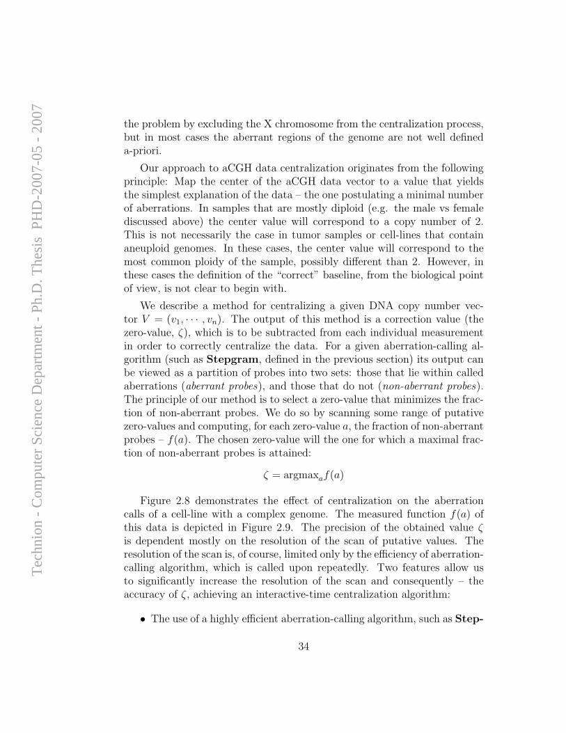
Our approach to aCGH data centralization originates from the followingprinciple: Map the center of the aCGH data vector to a value that yieldsthe simplest explanation of the data – the one postulating a minimal numberof aberrations. In samples that are mostly diploid (e.g. the male vs femalediscussed above) the center value will correspond to a copy number of 2.This is not necessarily the case in tumor samples or cell-lines that containaneuploid genomes. In these cases, the center value will correspond to themost common ploidy of the sample, possibly different than 2. However, inthese cases the definition of the “correct” baseline, from the biological pointof view, is not clear to begin with.
We describe a method for centralizing a given DNA copy number vec-tor V = (v1, · · · , vn). The output of this method is a correction value (thezero-value, ζ), which is to be subtracted from each individual measurementin order to correctly centralize the data. For a given aberration-calling al-gorithm (such as Stepgram, defined in the previous section) its output canbe viewed as a partition of probes into two sets: those that lie within calledaberrations (aberrant probes), and those that do not (non-aberrant probes).The principle of our method is to select a zero-value that minimizes the frac-tion of non-aberrant probes. We do so by scanning some range of putativezero-values and computing, for each zero-value a, the fraction of non-aberrantprobes – f(a). The chosen zero-value will the one for which a maximal frac-tion of non-aberrant probes is attained:
ζ = argmaxaf(a)
Figure 2.8 demonstrates the effect of centralization on the aberrationcalls of a cell-line with a complex genome. The measured function f(a) ofthis data is depicted in Figure 2.9. The precision of the obtained value ζis dependent mostly on the resolution of the scan of putative values. Theresolution of the scan is, of course, limited only by the efficiency of aberration-calling algorithm, which is called upon repeatedly. Two features allow usto significantly increase the resolution of the scan and consequently – theaccuracy of ζ, achieving an interactive-time centralization algorithm:
• The use of a highly efficient aberration-calling algorithm, such as Step-
34
Tec
hnio
n -
Com
pute
r Sc
ienc
e D
epar
tmen
t - P
h.D
. The
sis
PH
D-2
007-
05 -
200
7
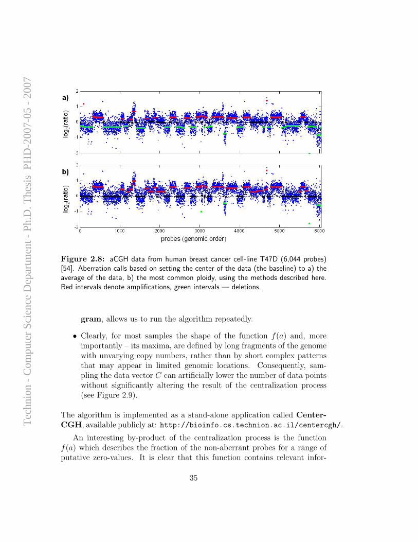
Figure 2.8: aCGH data from human breast cancer cell-line T47D (6,044 probes)[54]. Aberration calls based on setting the center of the data (the baseline) to a) theaverage of the data, b) the most common ploidy, using the methods described here.Red intervals denote amplifications, green intervals — deletions.
gram, allows us to run the algorithm repeatedly.
• Clearly, for most samples the shape of the function f(a) and, moreimportantly – its maxima, are defined by long fragments of the genomewith unvarying copy numbers, rather than by short complex patternsthat may appear in limited genomic locations. Consequently, sam-pling the data vector C can artificially lower the number of data pointswithout significantly altering the result of the centralization process(see Figure 2.9).
The algorithm is implemented as a stand-alone application called Center-CGH, available publicly at: http://bioinfo.cs.technion.ac.il/centercgh/.
An interesting by-product of the centralization process is the functionf(a) which describes the fraction of the non-aberrant probes for a range ofputative zero-values. It is clear that this function contains relevant infor-
35
Tec
hnio
n -
Com
pute
r Sc
ienc
e D
epar
tmen
t - P
h.D
. The
sis
PH
D-2
007-
05 -
200
7
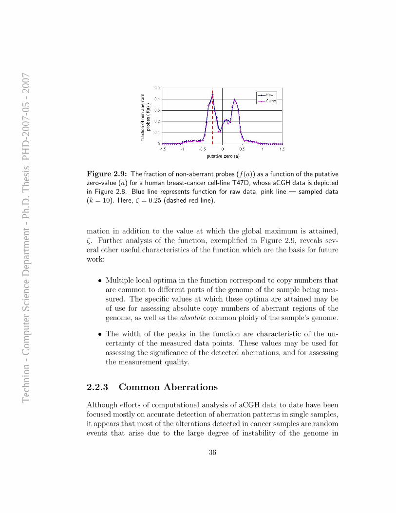
Figure 2.9: The fraction of non-aberrant probes (f(a)) as a function of the putativezero-value (a) for a human breast-cancer cell-line T47D, whose aCGH data is depictedin Figure 2.8. Blue line represents function for raw data, pink line — sampled data(k = 10). Here, ζ = 0.25 (dashed red line).
mation in addition to the value at which the global maximum is attained,ζ. Further analysis of the function, exemplified in Figure 2.9, reveals sev-eral other useful characteristics of the function which are the basis for futurework:
• Multiple local optima in the function correspond to copy numbers thatare common to different parts of the genome of the sample being mea-sured. The specific values at which these optima are attained may beof use for assessing absolute copy numbers of aberrant regions of thegenome, as well as the absolute common ploidy of the sample’s genome.
• The width of the peaks in the function are characteristic of the un-certainty of the measured data points. These values may be used forassessing the significance of the detected aberrations, and for assessingthe measurement quality.
2.2.3 Common Aberrations
Although efforts of computational analysis of aCGH data to date have beenfocused mostly on accurate detection of aberration patterns in single samples,it appears that most of the alterations detected in cancer samples are randomevents that arise due to the large degree of instability of the genome in
36
Tec
hnio
n -
Com
pute
r Sc
ienc
e D
epar
tmen
t - P
h.D
. The
sis
PH
D-2
007-
05 -
200
7
cancer cells, and do not necessarily have any direct influence on cellularfunction. However, it is long known that specific genomic alterations (such asones exemplified in Section 1.1.1) are observed frequently in certain types oftumors, and reflect common themes in cancer biology that have interpretable,causal ramifications. Hence, the task of identifying and mapping common,overlapping genomic aberrations across a sample set is of high importance;it can provide insight for the discovery of oncogenes, tumor suppressors, andthe mechanisms by which they drive cancer development.
A computational framework for identification and statistical characteri-zation of genomic aberrations that are common to multiple cancer samplesin a CGH data set, including several efficient algorithmic approaches withinthis framework, is described in the following paper [9]. Here I summarize themain contributions of this paper:
• A. Ben-Dor, D. Lipson, A. Tsalenko, M. Reimers, L.O. Baumbusch,M.T. Barrett, J.N. Weinstein, A. Borresen-Dale, and Z. Yakhini, “Frame-work for Identifying Common Aberrations in DNA Copy Num-ber Data”. Accepted for presentation at RECOMB ’07. (Appendix A.5)
Framework In a nutshell, the framework for identifying and statisticallyscoring aberrations that are reoccurring in multiple samples consists of foursteps.
1. Aberration Calling – Each of the samples’ data vector is analyzedindependently, and a set of aberrations (amplifications and deletions)is identified.
2. Listing candidate intervals - Given the collection of aberration setscalled for all samples, we construct a list of genomic intervals that willbe evaluated. We refer to these intervals as candidate intervals.
3. Scoring 〈candidate interval, sample〉 – In this step, we calculate astatistical significance score for each candidate interval with respect toeach sample.
4. Scoring candidate intervals – For each candidate interval, we com-bine the per-sample scores derived in the previous step into a com-prehensive score for the candidate interval and estimate its statistical
37
Tec
hnio
n -
Com
pute
r Sc
ienc
e D
epar
tmen
t - P
h.D
. The
sis
PH
D-2
007-
05 -
200
7
significance. In addition, we also identify for each candidate intervalthe set of samples that supports it.
At the end of the process, we list the top-scoring candidate intervals togetherwith their support sets. The framework is modular in nature, in the sensethat different algorithms and statistical models and methods can be used ineach of the different steps.
The starting point of the procedure of identifying statistically significantcommon aberrations is a set of aberrant segments for each sample. We as-sume that, independent of the particular aberration-calling algorithm, theset of aberration calls for a particular sample and a particular chromosomecan be represented by a step-function – a collection of discrete segments par-allel to the x-axis, that together span the entire chromosome. Formally, fora sample s, denote the length (in Mb) of the chromosome by `. A step-function Fs : [0, `] −→ R contains a segment for each aberration call (withthe appropriate boundaries and height), or segments of height zero for non-aberrant regions of the chromosome. An example of a suitable aberrationcalling algorithm, Stepgram [37], was described in Section 2.2.1.
Next we describe three algorithms based on the framework. For simplicity,we will describe only scores related to common amplifications, although itis clear that symmetric scores apply to common deletions. We denote byV = (v1, · · · , vn) the vector of DNA copy number data for a given sample.
Penterance Score A commonly-used measure for common aberrations isthe penetrance score, described in Section 1.1.4 and Figure 1.4. Although itis not a measure of statistical significance, it can be used to exemplify thedifferent steps of the process (following the aberration calling step):
2. Candidate intervals – For the penetrance score, candidate intervalsare defined simply as the positions of the probes in the aCGH array.
3. Scoring 〈interval, sample〉 For a given probe i and sample s theamplification penetrance score is defined as a binary score α(i, s) =1Fs(vi)>t for some threshold t.
4. Scoring candidate intervals The overall penetrance score for a givenprobe i is defined simply as α(i) =
∑s α(i, s). As noted before, this
score does not reflect any measure of statistical significance.
38
Tec
hnio
n -
Com
pute
r Sc
ienc
e D
epar
tmen
t - P
h.D
. The
sis
PH
D-2
007-
05 -
200
7
Context-Corrected Scores A variant of the penetrance score provides ameasure of statistical significance of the common aberration at the specifiedprobe. The significance is defined with respect to the genomic backgroundof each sample, as represented by the pattern of aberrations for each ofthe samples. In other words, given the specific set of aberration calls foreach sample, we wish to describe our “surprise” at seeing a specific set ofaberrations co-localized at the same genomic position. Note that the contextprovided for the score may be either genomic or chromosomal.
2. Candidate intervals – As before, the candidate intervals are definedas the positions of the probes in the aCGH array.
3. Scoring 〈interval, sample〉 The context-corrected score of a givenprobe i and sample s reflects the probability of finding a probe ofsimilar (or higher) amplitude given the context of the sample:
p(i, s) =|{vj ∈ V : Fs(vj) ≥ Fs(vi)}|
|V |.
4. Scoring candidate intervals Given a set of samples S of size m weseek the subset of samples that will provide maximal significance. As-sume, w.l.o.g., that p(i, 1) ≤ p(i, 2) ≤ . . . ≤ p(i, m). For the first ksamples, the probability of concurrently observing k or more scores ofprobability p = p(i, k) or lower is obtained using the Binomial distri-bution (since we’re interested in at least two samples, we ignore thefirst):
ρk(i) = Binom(k − 1, m− 1, p) =m−1∑
j=k−1
(m− 1
j
)pi(1− p)m−j−1
We define the score of I, to be the minimum of these scores over allvalues of k, namely,
ρ(i) = mink=2,...,m
ρk(i).
Although the context-corrected penetrance algorithm will clearly detectstatistically significant common aberrations that are affecting a single probe,its ability to detect larger significant aberrations is not guaranteed. In some
39
Tec
hnio
n -
Com
pute
r Sc
ienc
e D
epar
tmen
t - P
h.D
. The
sis
PH
D-2
007-
05 -
200
7
cases, a multi-probe common aberration may be significant as a whole, al-though the score of each single probe contained in the aberration may notshow statistical significance.
The third algorithm for identifying significant common aberrations ex-pands the concept of a context-corrected significance score to intervals thatare larger than a single probe. We do so by modifying the the second stepof the framework:
2. Candidate intervals – Consider a particular chromosome, c, and de-note by T = {[b1, e1], . . . , [bk, ek]} the set of all genomic intervals in cthat are called as aberrant in any of the samples. The set of candidateintervals in c is defined to be all intervals in T and intersections thereof,that is I = T ∪{t∩ s : t, s ∈ T}. Note that the size of I is quadratic ink, the number of called aberrations, and can be constructed in O(n).
Following this step, we score each candidate interval as was done for the pre-vious score (see Appendix A.5 for details). This final variant of the frameworkis named CoCoA (for Context-corrected Common Aberrations).
Application We demonstrate the application of the different algorithms ona set of 20 primary breast tumor samples [7]. Due to the relative homogeneityof this panel, we expected to encounter common aberrations typical of breastcancer. We first compared the three algorithms – simple penetrance, context-corrected penetrance, and CoCoA. Overall, the three algorithms detectedsimilar patterns, although the specific output contained obvious differences.Figure 2.10 depicts the output of the three algorithms for Chromosome 9 ofthe breast tumor dataset.
The most prominent common aberrations in the chromosome shown areclearly the large amplification between 110-120Mb and the smaller deletionat 95Mb, both of which were detected by all algorithms. The results of thesimple penetrance method, which is a non-statistical method, can be inter-preted loosely based on setting of some arbitrary threshold. It is clear that asignificant part of the genome can be considered to contain common aberra-tions if that method is used. The context-corrected penetrance method givesimproved output in the sense that only very specific parts of the chromosomeare deemed to contain common aberrations, based on a very modest thresholdρ(I) < 10−3. Clearly, from the biological point of view, specific output of this
40
Tec
hnio
n -
Com
pute
r Sc
ienc
e D
epar
tmen
t - P
h.D
. The
sis
PH
D-2
007-
05 -
200
7
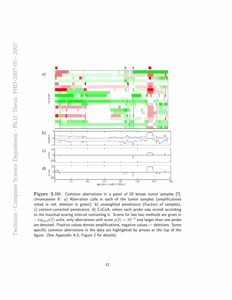
Figure 2.10: Common aberrations in a panel of 20 breast tumor samples [7],chromosome 9: a) Aberration calls in each of the tumor samples (amplificationsnoted in red, deletion in green); b) unweighted penetrance (fraction of samples),c) context-corrected penetrance, d) CoCoA, where each probe was scored accordingto the maximal-scoring interval containing it. Scores for last two methods are given in− log10 ρ(I) units, only aberrations with score ρ(I) < 10−3 and larger than one probeare denoted. Positive values denote amplifications, negative values — deletions. Somespecific common aberrations in the data are highlighted by arrows at the top of thefigure. (See Appendix A.5, Figure 2 for details).
41
Tec
hnio
n -
Com
pute
r Sc
ienc
e D
epar
tmen
t - P
h.D
. The
sis
PH
D-2
007-
05 -
200
7
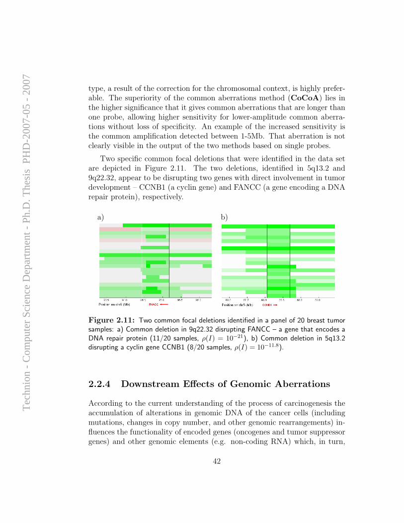
type, a result of the correction for the chromosomal context, is highly prefer-able. The superiority of the common aberrations method (CoCoA) lies inthe higher significance that it gives common aberrations that are longer thanone probe, allowing higher sensitivity for lower-amplitude common aberra-tions without loss of specificity. An example of the increased sensitivity isthe common amplification detected between 1-5Mb. That aberration is notclearly visible in the output of the two methods based on single probes.
Two specific common focal deletions that were identified in the data setare depicted in Figure 2.11. The two deletions, identified in 5q13.2 and9q22.32, appear to be disrupting two genes with direct involvement in tumordevelopment – CCNB1 (a cyclin gene) and FANCC (a gene encoding a DNArepair protein), respectively.
a) b)
Figure 2.11: Two common focal deletions identified in a panel of 20 breast tumorsamples: a) Common deletion in 9q22.32 disrupting FANCC – a gene that encodes aDNA repair protein (11/20 samples, ρ(I) = 10−21), b) Common deletion in 5q13.2disrupting a cyclin gene CCNB1 (8/20 samples, ρ(I) = 10−11.8).
2.2.4 Downstream Effects of Genomic Aberrations
According to the current understanding of the process of carcinogenesis theaccumulation of alterations in genomic DNA of the cancer cells (includingmutations, changes in copy number, and other genomic rearrangements) in-fluences the functionality of encoded genes (oncogenes and tumor suppressorgenes) and other genomic elements (e.g. non-coding RNA) which, in turn,
42
Tec
hnio
n -
Com
pute
r Sc
ienc
e D
epar
tmen
t - P
h.D
. The
sis
PH
D-2
007-
05 -
200
7
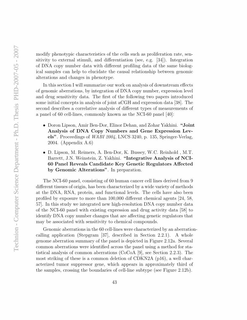
modify phenotypic characteristics of the cells such as proliferation rate, sen-sitivity to external stimuli, and differentiation (see, e.g. [34]). Integrationof DNA copy number data with different profiling data of the same biolog-ical samples can help to elucidate the causal relationship between genomicalterations and changes in phenotype.
In this section I will summarize our work on analysis of downstream effectsof genomic aberrations, by integration of DNA copy number, expression leveland drug sensitivity data. The first of the following two papers introducedsome initial concepts in analysis of joint aCGH and expression data [38]. Thesecond describes a correlative analysis of different types of measurements ofa panel of 60 cell-lines, commonly known as the NCI-60 panel [40]:
• Doron Lipson, Amir Ben-Dor, Elinor Dehan, and Zohar Yakhini. “JointAnalysis of DNA Copy Numbers and Gene Expression Lev-els”. Proceedings of WABI 2004, LNCS 3240, p. 135, Springer-Verlag,2004. (Appendix A.6)
• D. Lipson, M. Reimers, A. Ben-Dor, K. Bussey, W.C. Reinhold , M.T.Barrett, J.N. Weinstein, Z. Yakhini. “Integrative Analysis of NCI-60 Panel Reveals Candidate Key Genetic Regulators Affectedby Genomic Alterations”. In preparation.
The NCI-60 panel, consisting of 60 human cancer cell lines derived from 9different tissues of origin, has been characterized by a wide variety of methodsat the DNA, RNA, protein, and functional levels. The cells have also beenprofiled by exposure to more than 100,000 different chemical agents [24, 58,57]. In this study we integrated new high-resolution DNA copy number dataof the NCI-60 panel with existing expression and drug activity data [58] toidentify DNA copy number changes that are affecting genetic regulators thatmay be associated with sensitivity to chemical compounds.
Genomic aberrations in the 60 cell-lines were characterized by an aberration-calling application (Stepgram [37], described in Section 2.2.1). A wholegenome aberration summary of the panel is depicted in Figure 2.12a. Severalcommon aberrations were identified across the panel using a method for sta-tistical analysis of common aberrations (CoCoA [9], see Section 2.2.3). Themost striking of these is a common deletion of CDKN2A (p16), a well char-acterized tumor suppressor gene, which appears in approximately third ofthe samples, crossing the boundaries of cell-line subtype (see Figure 2.12b).
43
Tec
hnio
n -
Com
pute
r Sc
ienc
e D
epar
tmen
t - P
h.D
. The
sis
PH
D-2
007-
05 -
200
7
Figure 2.12: a) NCI-60 whole genome aberration summary. Aberrations detectedwith Stepgram [37]: Red color indicates amplified interval, green color indicates deletedinterval. Rows represent the 60 cell lines (BR: breast, CNS: central nervous system,CO: colon, LC: lung, LE: leukemia, ME: melanoma, OV: ovarian, PR: prostate, RE:renal). b) Common deletion detected in 9p, hitting CDKN2A (p16).
44
Tec
hnio
n -
Com
pute
r Sc
ienc
e D
epar
tmen
t - P
h.D
. The
sis
PH
D-2
007-
05 -
200
7
To measure the effect of genomic aberrations on expression levels wecompare the DNA copy numbers and expression levels of each individual geneacross the panel. To improve the accuracy of the DNA copy number estimatefor a given gene at a given sample we use the processed aberration leveldescribed by the step-function at the genomic locus of the gene, rather thanits raw probe measurement. The effect of gene copy number on transcriptexpression can be demonstrated at different levels:
• At the single gene/sample level: For each gene g and sample s wehave two values: DNA copy number (from the processed aCGH data)– d(g, s), and expression level – e(g, s). Comparing these paired valuesover all genes and samples (over 106 pairs) demonstrates a significantcorrelation. However, overall, changes in DNA copy number account foronly 5-10% of the variance in the expression levels (see Figure 2.13a).
• At the single gene level, across the sample set: For each gene g wehave two vectors ~d(g) and ~e(g) describing the matched processed DNAcopy number and expression level measurements across the sample set.The correlation between these two vectors represents the effect of DNAcopy numbers on expression levels for this gene. The distribution ofall correlation values shows a significant shift, with respect to the nulldistribution (see Figure 2.13b). Correlation may be assessed using dif-ferent scores, most commonly:
– Pearson’s correlation coefficient is a measure of the linear depen-dency between the two vectors, and is the most commonly usedcorrelation score (e.g. [54]). However, this score is highly sensitiveto outliers.
– Partitioning the samples into two subsets, according to the exis-tence of an gain or loss at the DNA level, enables using a Student’st-test to score the difference in expression levels between these twosubsets (e.g. [29]).
– Non-parametric tests, such as Spearman’s correlation coefficient,or MDP [38].
• At the genome level, the presence of over- or under-expressed genes maybe compared to the existence of genomic amplifications or deletions,
45
Tec
hnio
n -
Com
pute
r Sc
ienc
e D
epar
tmen
t - P
h.D
. The
sis
PH
D-2
007-
05 -
200
7
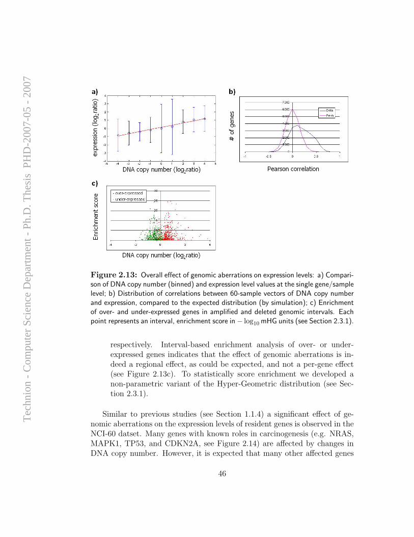
Figure 2.13: Overall effect of genomic aberrations on expression levels: a) Compari-son of DNA copy number (binned) and expression level values at the single gene/samplelevel; b) Distribution of correlations between 60-sample vectors of DNA copy numberand expression, compared to the expected distribution (by simulation); c) Enrichmentof over- and under-expressed genes in amplified and deleted genomic intervals. Eachpoint represents an interval, enrichment score in − log10 mHG units (see Section 2.3.1).
respectively. Interval-based enrichment analysis of over- or under-expressed genes indicates that the effect of genomic aberrations is in-deed a regional effect, as could be expected, and not a per-gene effect(see Figure 2.13c). To statistically score enrichment we developed anon-parametric variant of the Hyper-Geometric distribution (see Sec-tion 2.3.1).
Similar to previous studies (see Section 1.1.4) a significant effect of ge-nomic aberrations on the expression levels of resident genes is observed in theNCI-60 datset. Many genes with known roles in carcinogenesis (e.g. NRAS,MAPK1, TP53, and CDKN2A, see Figure 2.14) are affected by changes inDNA copy number. However, it is expected that many other affected genes
46
Tec
hnio
n -
Com
pute
r Sc
ienc
e D
epar
tmen
t - P
h.D
. The
sis
PH
D-2
007-
05 -
200
7
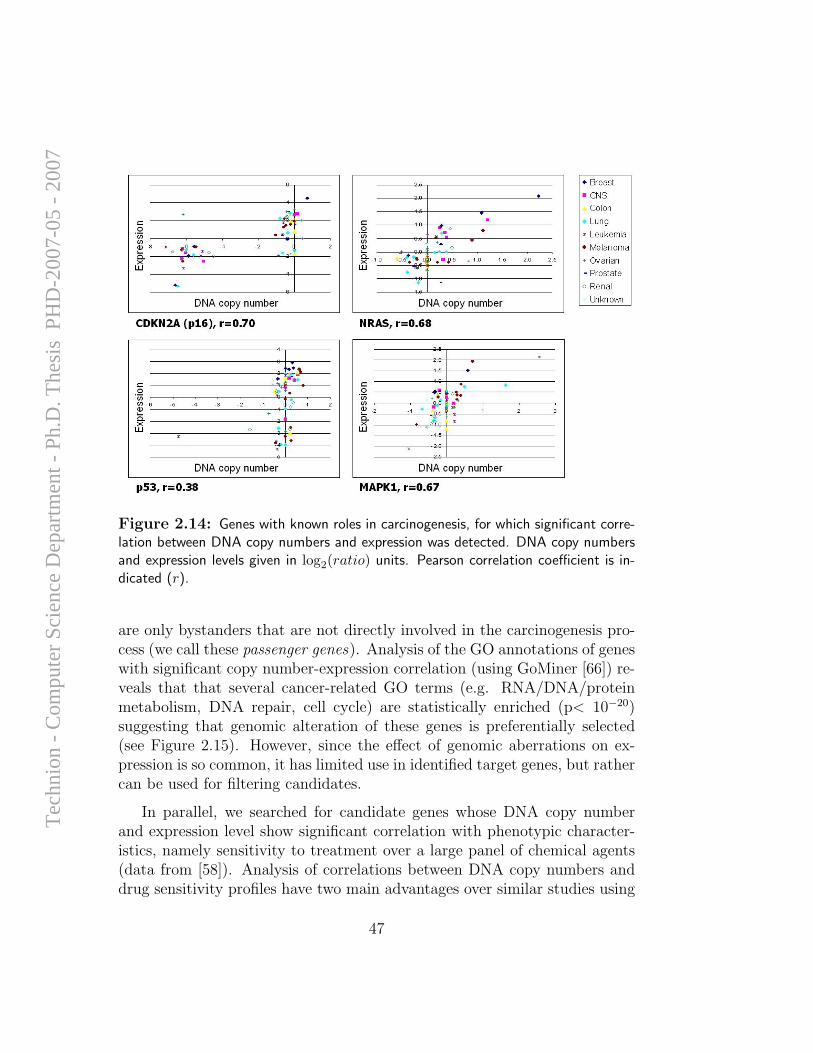
Figure 2.14: Genes with known roles in carcinogenesis, for which significant corre-lation between DNA copy numbers and expression was detected. DNA copy numbersand expression levels given in log2(ratio) units. Pearson correlation coefficient is in-dicated (r).
are only bystanders that are not directly involved in the carcinogenesis pro-cess (we call these passenger genes). Analysis of the GO annotations of geneswith significant copy number-expression correlation (using GoMiner [66]) re-veals that that several cancer-related GO terms (e.g. RNA/DNA/proteinmetabolism, DNA repair, cell cycle) are statistically enriched (p< 10−20)suggesting that genomic alteration of these genes is preferentially selected(see Figure 2.15). However, since the effect of genomic aberrations on ex-pression is so common, it has limited use in identified target genes, but rathercan be used for filtering candidates.
In parallel, we searched for candidate genes whose DNA copy numberand expression level show significant correlation with phenotypic character-istics, namely sensitivity to treatment over a large panel of chemical agents(data from [58]). Analysis of correlations between DNA copy numbers anddrug sensitivity profiles have two main advantages over similar studies using
47
Tec
hnio
n -
Com
pute
r Sc
ienc
e D
epar
tmen
t - P
h.D
. The
sis
PH
D-2
007-
05 -
200
7

Fig
ure
2.1
5:
GO
termen
richm
ent
analysis
ofsign
ifican
tlycorrelated
genes
(r>
0.32).
All
GO
terms
with
signifi
cant
enrich
men
t(p
<10−
8)are
colored,darker
coloredterm
sare
more
signifi
cantly
enrich
ed.
Most
signifi
cant
terms
inclu
de:
RN
Am
etabolism
(p<
10−
42),
DN
Am
etabolism
(p<
10−
30),
DN
Arep
air(p
<10−
24),
proteintran
sport
(p<
10−
28),
intracellu
lartran
sport
(p<
10−
29),
proteinm
etabolism
(p<
10−
25)
and
cellcycle
((p<
10−
21).
48
Tec
hnio
n -
Com
pute
r Sc
ienc
e D
epar
tmen
t - P
h.D
. The
sis
PH
D-2
007-
05 -
200
7
expression level data alone. First, the DNA copy numbers, which are basedon a pre-processing aberration-calling procedure, are expected to be morereliable than the noisier expression data (where single, or few, measurementsare typically used per gene). Second, since genomic aberrations are believedto be initial events (i.e. they do not affect each other) our ability to dis-cover causal relationships between aberrations and changes in phenotype isincreased. We calculated correlation between copy number data from theentire genome to a selected panel of 1,400 chemical compounds that wereselected from the database (see [58]). The correlation patterns with a sub-set of these compounds, with known mechanisms of action, are depicted inFigure 2.16. Focusing on the high-scoring correlations we identified a smallnumber of putative genetic regulators whose transcription levels are signif-icantly affected by genomics aberrations, and that appear to be associatedwith changes in sensitivity to specific chemical compounds. For example, thedeletion of CDKN2A in many of the cell-lines is associated with increasedsensitivity to chemical agents such as Cytarabine. The implication of MITFas a lineage survival oncogene [22], as well as the related SOX10, are alsoidentified by our approach (see Figure 2.17). Current work is centered onsuggesting possible control mechanisms of putative genetic regulators, andvalidation of some these regulators by means of specific siRNA experiments.
2.2.5 DNA Replication Patterns
Although the most common application of DNA copy number measurementis clearly in detection of aberrations in cancer genomes, there are severaladditional applications that can benefit from the aCGH platform. For ex-ample, different developmental disorders, such as Down’s Syndrome, resultfrom abnormal changes in DNA copy number. Here I will describe a differentapplication of aCGH involving an additional biological state in which varia-tions in DNA copy number are encountered – the replication of DNA duringcell cycle.
Replication of the genome during the S phase of the cell-cycle is a highlyregulated process. Recent studies of the replication timing patterns in thegenomes of drosophila and human [44, 65] demonstrated significant correla-tion between replication timing and transcriptional activity of encoded genes,although there are many genes that do not fit this scheme. In addition, littleis known about the genomic organization of the replication time zones. In a
49
Tec
hnio
n -
Com
pute
r Sc
ienc
e D
epar
tmen
t - P
h.D
. The
sis
PH
D-2
007-
05 -
200
7
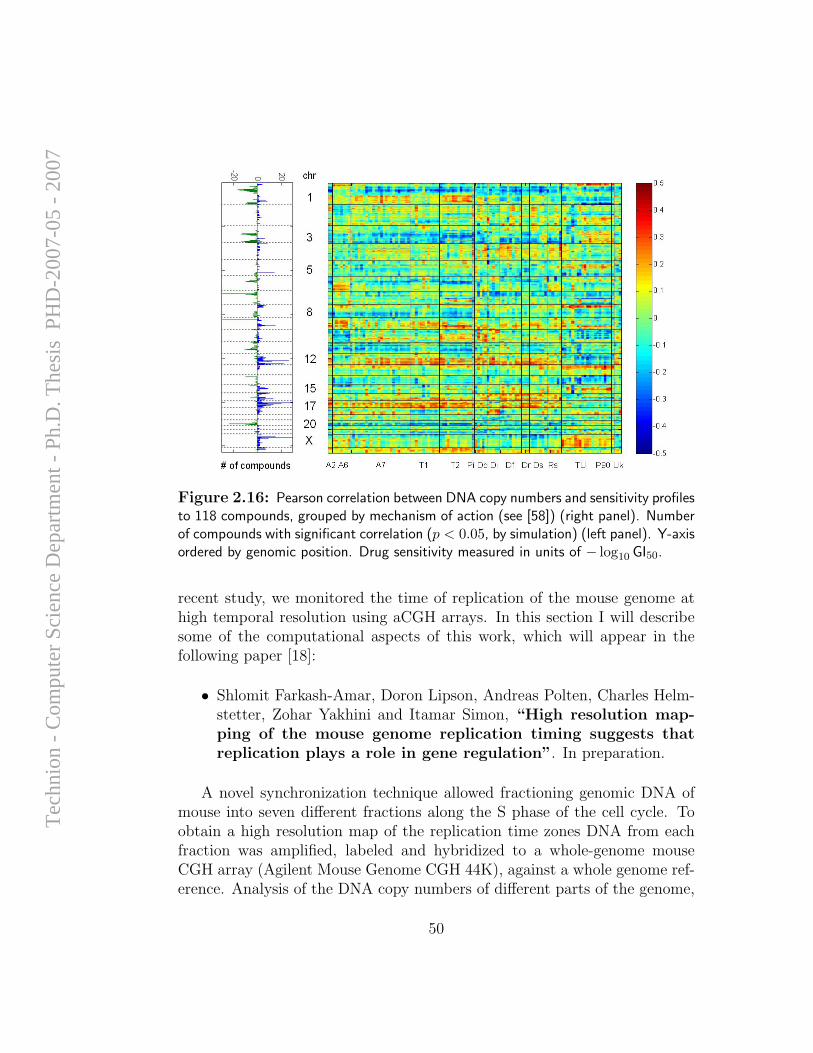
Figure 2.16: Pearson correlation between DNA copy numbers and sensitivity profilesto 118 compounds, grouped by mechanism of action (see [58]) (right panel). Numberof compounds with significant correlation (p < 0.05, by simulation) (left panel). Y-axisordered by genomic position. Drug sensitivity measured in units of − log10 GI50.
recent study, we monitored the time of replication of the mouse genome athigh temporal resolution using aCGH arrays. In this section I will describesome of the computational aspects of this work, which will appear in thefollowing paper [18]:
• Shlomit Farkash-Amar, Doron Lipson, Andreas Polten, Charles Helm-stetter, Zohar Yakhini and Itamar Simon, “High resolution map-ping of the mouse genome replication timing suggests thatreplication plays a role in gene regulation”. In preparation.
A novel synchronization technique allowed fractioning genomic DNA ofmouse into seven different fractions along the S phase of the cell cycle. Toobtain a high resolution map of the replication time zones DNA from eachfraction was amplified, labeled and hybridized to a whole-genome mouseCGH array (Agilent Mouse Genome CGH 44K), against a whole genome ref-erence. Analysis of the DNA copy numbers of different parts of the genome,
50
Tec
hnio
n -
Com
pute
r Sc
ienc
e D
epar
tmen
t - P
h.D
. The
sis
PH
D-2
007-
05 -
200
7
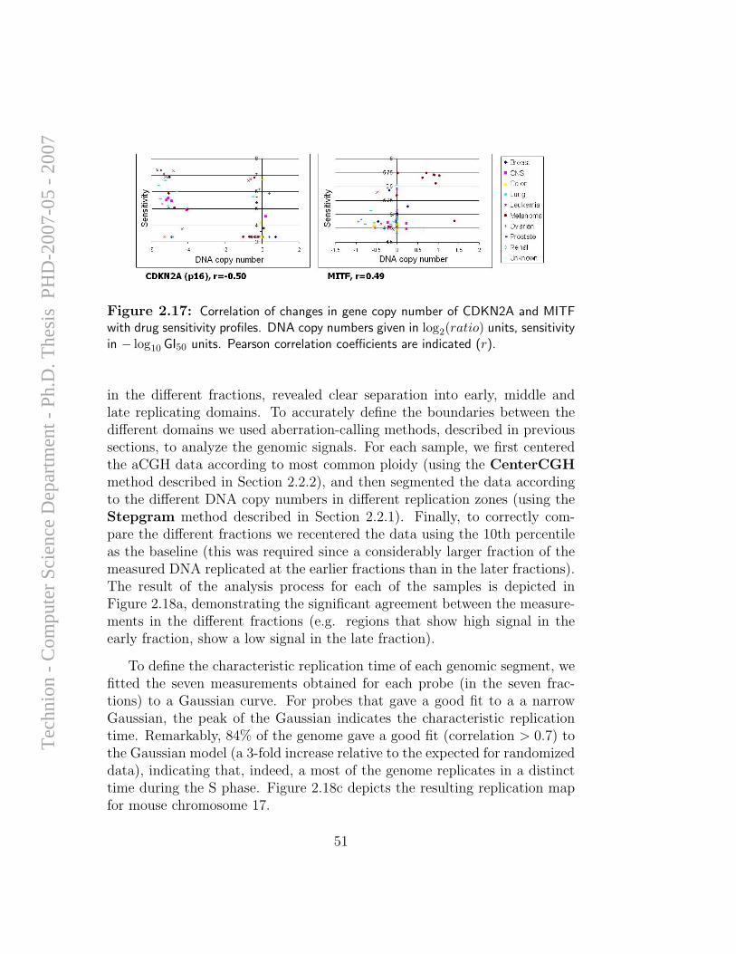
Figure 2.17: Correlation of changes in gene copy number of CDKN2A and MITFwith drug sensitivity profiles. DNA copy numbers given in log2(ratio) units, sensitivityin − log10 GI50 units. Pearson correlation coefficients are indicated (r).
in the different fractions, revealed clear separation into early, middle andlate replicating domains. To accurately define the boundaries between thedifferent domains we used aberration-calling methods, described in previoussections, to analyze the genomic signals. For each sample, we first centeredthe aCGH data according to most common ploidy (using the CenterCGHmethod described in Section 2.2.2), and then segmented the data accordingto the different DNA copy numbers in different replication zones (using theStepgram method described in Section 2.2.1). Finally, to correctly com-pare the different fractions we recentered the data using the 10th percentileas the baseline (this was required since a considerably larger fraction of themeasured DNA replicated at the earlier fractions than in the later fractions).The result of the analysis process for each of the samples is depicted inFigure 2.18a, demonstrating the significant agreement between the measure-ments in the different fractions (e.g. regions that show high signal in theearly fraction, show a low signal in the late fraction).
To define the characteristic replication time of each genomic segment, wefitted the seven measurements obtained for each probe (in the seven frac-tions) to a Gaussian curve. For probes that gave a good fit to a a narrowGaussian, the peak of the Gaussian indicates the characteristic replicationtime. Remarkably, 84% of the genome gave a good fit (correlation > 0.7) tothe Gaussian model (a 3-fold increase relative to the expected for randomizeddata), indicating that, indeed, a most of the genome replicates in a distincttime during the S phase. Figure 2.18c depicts the resulting replication mapfor mouse chromosome 17.
51
Tec
hnio
n -
Com
pute
r Sc
ienc
e D
epar
tmen
t - P
h.D
. The
sis
PH
D-2
007-
05 -
200
7

Figure 2.18: Replication time zones in the mouse genome, Chromosome 17: a)DNA copy number measurements from 7 fractions along the S phase of the cell cycle,red lines denote step-function; b) Example of processed measurements for 4 genomicloci across the 7 fractions, fitted to Gaussian curves; c) Positions of peaks of Gaussiancurves define the replication map of the chromosome.
Subsequently, we used the newly-measured replication time landscape tocharacterize the properties of the genomic replication zones and to explorethe correlations between replication times and gene transcription. A paperdescribing the biological results of this study is in preparation [18].
52
Tec
hnio
n -
Com
pute
r Sc
ienc
e D
epar
tmen
t - P
h.D
. The
sis
PH
D-2
007-
05 -
200
7
2.3 Additional Results
2.3.1 Enrichment Analysis
Many applications in computational biology require statistical assessmentof the degree of enrichment of elements from one particular subset A in adifferent subset B, within a pre-specified set of elements. For example, givena set of promoter sequences we can define A to be the subset of sequencescontaining a particular motif, and B to be the subset of sequences to which aparticular transcription factor (TF) physically binds to in a ChIP (ChromatinImmuno-Precipitation) experiment. Significant enrichment of elements of Awithin B (or vice-versa) may indicate that the transcription factor recognizesthe sequence motif as a physical binding site in the DNA (e.g., [25]).
Statistical scoring of enrichment is typically done using the Hyper-Geometric(HG) distribution, or its derivative – Fisher’s exact test [20]. However, con-sider the following variant of the problem: Instead of a specific subset B, weare given a ranking of the elements in the set, and the enrichment problem ismodified accordingly: Are elements of A significantly enriched at the top ofthe ranked list. Practically, this modified version of the enrichment problemis one that typically appears in biological settings. For example, in the abovescenario the ChIP experiment would most likely result in a ranking of thesequences by the level of binding of the transcription factor, rather than aclear partition into binding and non-binding subsets.
A simple solution to the “ranked enrichment” problem is to partition theranked list into two subsets using an arbitrary threshold, thereby revertingto the original variant of the problem. However, in many cases the choice ofthis cutoff is unclear. The following paper describes a statistical method forenrichment analysis of ranked lists, in the context of searching for sequencemotifs [17]. Here I will summarize the computational aspects of this method:
• Eran Eden, Doron Lipson, Sivan Yogev, and Zohar Yakhini. “Dis-covering Motifs in Ranked Lists of DNA Sequences”. PLoSComputational Biology, 3(3):e39, 2007. (Appendix A.7)
Let N be the total number of elements in a given set (the promotersequences), B – the size of a given subset (sequences that the to which theTF binds), and n – the size of the target subset (sequences that contain a
53
Tec
hnio
n -
Com
pute
r Sc
ienc
e D
epar
tmen
t - P
h.D
. The
sis
PH
D-2
007-
05 -
200
7
specific motif). If X is a random variable describing the size of the overlapbetween the two subsets then the probability of finding b or more elementsin the overlap is given by the tail probability of the HG distribution:
Prob(X ≥ b) = HGT(b; N, B, n) =
min(n,B)∑i=b
(ni
)(N−nB−i
)(NB
) .
Now, consider a set of ranked elements (by order of TF binding) andsome binary labeling of the set λ = λ1, ..., λN ∈ {0, 1}N . The binary labelsrepresent the attribute (motif occurrence). The minimum Hyper-Geometric(mHG) score is defined as:
mHG(λ) = min1≤n<N
HGT(bn(λ); N, B, n),
where bn(λ) =∑n
i=1 λi (by definition, B = bN(λ)). In words, the mHG scorereflects the surprise of seeing the observed density of 1’s at the top of thelist under the null assumption that all configurations of 1’s in the vector areequiprobable.
Clearly, despite the fact that the mHG score is based on the HG distribu-tion, this score itself is not a probability function due to the use of multipletesting. Interestingly, the exact p-value of a given mHG score can be cal-culated by dynamic programming. This approach is related to previouslydescribed work on calculation of exact p-values of other combinatorial scores[8].
Note that the mHG score depends solely on the content of label vector λ.Set N and B, and consider the space of all binary label vectors with B 1’s andN −B 0’s: Λ = {0, 1}(N−B,B). Assume that we are given a vector λ0 ∈ Λ, forwhich we calculate the mHG score mHG(λ0) = p. We would like to determinepval(p) = Prob(mHG(λ) ≤ p) under a uniform distribution of vectors in Λ.Given a mHG score p we calculate pval(p) by means of path counting. Thespace of all label vectors Λ is represented as a two-dimensional grid rangingfrom (0, 0) at the bottom-left to (N, B) at the top-right. Each specific labelvector λ ∈ Λ is represented by a path (0, 0) → (N, B) composed of N distinctsteps, where the ith step is (1, 0) if λi = 0 and (1, 1) if λi = 1 (see Figure 2.19).Each point (n, b) on the grid corresponds to a threshold n, and the respectivevalue b = bn(λ). It can therefore be associated with a specific HGT score:HGTn(λ) = HGT(bn(λ); N, B, n). A subset of the points on the grid can
54
Tec
hnio
n -
Com
pute
r Sc
ienc
e D
epar
tmen
t - P
h.D
. The
sis
PH
D-2
007-
05 -
200
7
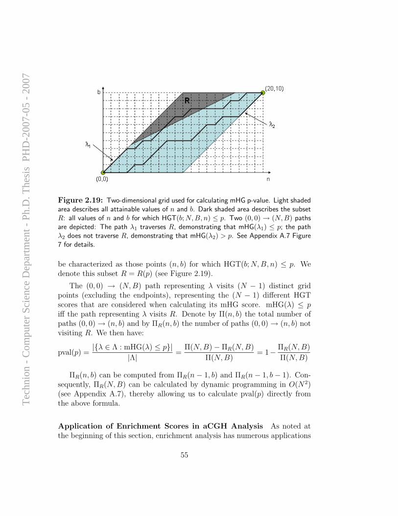
Figure 2.19: Two-dimensional grid used for calculating mHG p-value. Light shadedarea describes all attainable values of n and b. Dark shaded area describes the subsetR: all values of n and b for which HGT(b;N,B, n) ≤ p. Two (0, 0) → (N,B) pathsare depicted: The path λ1 traverses R, demonstrating that mHG(λ1) ≤ p; the pathλ2 does not traverse R, demonstrating that mHG(λ2) > p. See Appendix A.7 Figure7 for details.
be characterized as those points (n, b) for which HGT(b; N, B, n) ≤ p. Wedenote this subset R = R(p) (see Figure 2.19).
The (0, 0) → (N, B) path representing λ visits (N − 1) distinct gridpoints (excluding the endpoints), representing the (N − 1) different HGTscores that are considered when calculating its mHG score. mHG(λ) ≤ piff the path representing λ visits R. Denote by Π(n, b) the total number ofpaths (0, 0) → (n, b) and by ΠR(n, b) the number of paths (0, 0) → (n, b) notvisiting R. We then have:
pval(p) =|{λ ∈ Λ : mHG(λ) ≤ p}|
|Λ|=
Π(N, B)− ΠR(N, B)
Π(N, B)= 1− ΠR(N, B)
Π(N, B)
ΠR(n, b) can be computed from ΠR(n− 1, b) and ΠR(n− 1, b− 1). Con-sequently, ΠR(N, B) can be calculated by dynamic programming in O(N2)(see Appendix A.7), thereby allowing us to calculate pval(p) directly fromthe above formula.
Application of Enrichment Scores in aCGH Analysis As noted atthe beginning of this section, enrichment analysis has numerous applications
55
Tec
hnio
n -
Com
pute
r Sc
ienc
e D
epar
tmen
t - P
h.D
. The
sis
PH
D-2
007-
05 -
200
7
in computational biology. In aCGH data analysis, a particularly interest-ing application is the identification of significantly enriched intervals. Forexample, given a set of amplified genomic segments and a set of ranked ele-ments with genomic positions (e.g. over-expressed genes) we can determinewhich of the amplified segments is significantly enriched in over-expressedgenes. Using mHG, we do not need to predefine an arbitrary threshold forover-expression. An example of this application is given in Figure 2.13c,demonstrating that amplified genomic segments indeed tend to be enrichedin over-expressed genes, and deleted segments — in under-expressed genes.Interestingly, even if we have no DNA copy number data available, we canuse enrichment analysis of over- and under-expressed genes to predict whichgenomic segments are amplified or deleted – by considering all intervals, andpicking out the most significantly enriched ones.
56
Tec
hnio
n -
Com
pute
r Sc
ienc
e D
epar
tmen
t - P
h.D
. The
sis
PH
D-2
007-
05 -
200
7

Chapter 3
Discussion
The development of aCGH, and more specifically – oligonucleotide aCGH,in recent years dramatically increased the resolution at which we can studythe characteristics of genomic rearrangements in various biological settings.The impact is most significant on our ability to accurately map copy numberchanges in cancer genomes, since these cells commonly display different lev-els of genomic rearrangement. The appearance and accumulation of genomicaberrations are believed to be central events in the process of tumor initiationand progression. High resolution CGH arrays allow us to detect increasinglyfocused aberrations, and to pinpoint breakpoints of genomic rearrangementsat an accuracy that may allow the identification of new genomic constructs.Latest development of aCGH technology enables probing whole genomes atorder of Kbp average resolution. In combination with high-definition arrays,genomic breakpoints can theoretically be mapped at a resolution that ap-proaches single bases. Practically, however, the resolution at which genomicbreakpoints can be mapped may be limited by the DNA sequence itself, sincethese tend to occur at low-complexity repetitive sequence (see Section 2.1.2).Time will tell if this inherent limitation of aCGH resolution can be overcome.
Closely following the development of CGH arrays, many computationaltools for characterizing the aberration structure of cancer genomes based onDNA copy number data were developed. Currently, given the high qual-ity data that is acquired using commercial arrays, many of the methods foraberration-calling produce satisfactory and reproducible descriptions of thegenomic aberration patterns. In our work, we put an emphasis on develop-ing an aberration-calling method that is highly efficient, while maintaining
57
Tec
hnio
n -
Com
pute
r Sc
ienc
e D
epar
tmen
t - P
h.D
. The
sis
PH
D-2
007-
05 -
200
7
the accuracy of the results. As a consequence, Stepgram (described inSection 2.2.1) is one of the fastest methods for analysis of raw DNA copynumber data, demonstrating running times of single seconds even for largearrays. The efficiency of the algorithm is important not only due to the rapidincrease in array capacity (arrays with millions of probes are now available)and sample set size (hundreds of samples in single studies), but also in orderto enable efficient higher-level methods that may use the aberration-callingstep as a subroutine (e.g. CenterCGH and algorithms for detecting com-mon aberrations).
As the basic task of fitting the best aberration pattern to a given aCGHdata vector has been given adequate solutions, current work on aCGH sig-nal analysis attempts to address second-order obstructive issues. Such issuesinclude drifts in the aCGH signal, heterogeneous samples, and high-orderaneuploidy (cells having >2 copies of the entire genome). Methods un-der development also attempt to incorporate sequence information into theaberration-calling strategy, e.g. by increasing the likelihood of breakpointsat low-complexity sequence. Another aspect of single-sample data analysisinvolves the task of extracting absolute DNA copy numbers from the aCGHsignal, a task which is more difficult than could initially be expected.
However, as described in this work, accurate identification of genomicaberrations is only the initial step in uncovering specific genomic alterationevents that are significant to the process of tumor development. Little hasbeen done, on the computational front, to fully exploit the power of largepanels of tumors characterized by aCGH. Here I described a new tool thatwe developed for identifying aberrations that significantly reoccur in tumorsamples (CoCoA, Section 2.2.3), but there is still a significant need for toolsfor performing related tasks. For example, although these issues have beendeeply explored for expression profiling data, no significant work has beenpublished to date (to the best of my knowledge) concerning machine learningaspects of aCGH analysis such as: Identification of genomic aberrations thatdiscriminate between tumor subtypes, classification of tumor samples basedon their aberration patterns, or class discovery within heterogeneous classesof tumor based on genomic aberrations. Moreover, little has been done tocomprehensively characterize the association between different genomic alter-ations based on aCGH data, which may provide significant biological insight.
In the realm of integrative analysis of DNA copy number data togetherwith parallel information at the transcript, protein, and pharmacological lev-
58
Tec
hnio
n -
Com
pute
r Sc
ienc
e D
epar
tmen
t - P
h.D
. The
sis
PH
D-2
007-
05 -
200
7
els, I have described some preliminary results from our work on identificationof putative genomic regulators affected by genomic aberrations based on theNCI-60 cell-line panel (Section 2.2.4). Similar studies incorporating mostlygene expression profile data have been performed on sets of tumors fromdifferent cancer subtypes. The general conclusion that seems to be the com-mon outcome of these studies is that DNA copy number changes significantlyinfluence gene expression levels wherever they appear in the genome. Thisinsight strengthens the hypothesis that the effect of genomic aberrations onthe phenotype of tumor cells manifests via altered transcript levels, albeitit weakens the utility of this correlation in identifying the target genes. Inconsequence, it appears that aCGH and expression data must be integratedwith additional data sources (such as phenotypic data) in order to fully real-ize their potential. In addition, the influence of changes in DNA copy numberon other genomic elements (such as regulatory factors, and non-coding RNA)has yet to be explored.
Although changes in DNA copy number are most typically associatedwith malignancy, recent work [59, 56, 61] has unveiled that DNA copy num-ber variations (CNVs) are actually a common source of genetic diversity inthe general population, and that these variations may possibly have directfunctional effects. As a consequence, it is likely that analysis of DNA copynumber using aCGH may become a popular method for genotype profilingstudies, in addition to its central place in oncogenomic analysis. Addition-ally, other uses of aCGH are possible, such as studies of genome replicationpatterns (as described in Section 2.2.5), DNA methylation patterns, etc.
As a final note I would like to point to the recent initiation of the pilotphase of The Cancer Genome Atlas (TCGA, see http://cancergenome.nih.gov/)as a near-future source of high quality and large volume of DNA copy num-ber data from various subtypes of tumors. The Cancer Genome Atlas is acomprehensive and coordinated effort by the NCI and NHGRI to acceleratethe understanding of the molecular basis of cancer through the applicationof multiple genome analysis technologies on a large and carefully-regulatedcohort of tumor samples. In its initial phase this project is expected to collectand characterize hundreds of samples of lung, brain (glioblastoma), and ovar-ian tumors. Thereby it will provide a significant database on which methodsfor extracting biological meaning from DNA copy number data can be ef-ficiently developed and through which significant discoveries can be made,affecting cancer diagnostics and therapeutics.
59
Tec
hnio
n -
Com
pute
r Sc
ienc
e D
epar
tmen
t - P
h.D
. The
sis
PH
D-2
007-
05 -
200
7

60
Tec
hnio
n -
Com
pute
r Sc
ienc
e D
epar
tmen
t - P
h.D
. The
sis
PH
D-2
007-
05 -
200
7

Bibliography
[1] Agilent Technologies. CGH Analytics 3.2, 2005.
[2] A.J. Aguirre, C. Brennan, G. Bailey, R. Sinha, B. Feng, C. Leo,Y. Zhang, J. Zhang, J.D. Gans, N. Bardeesy, C. Cauwels, C. Cordon-Cardo, M.S. Redston, R.A. DePinho, and L. Chin. High-resolutioncharacterization of the pancreatic adenocarcinoma genome. PNAS,101(24):9067–72, 2004.
[3] S.F. Altschul, W. Gish, W. Miller, E.W. Myers, and D.J. Lipman. Basiclocal alignment search tool. J. Mol. Biol., 215(3):403–410, 1990.
[4] C. Baldwin, C. Garnis, L. Zhang, M.P. Rosin, and W.L. Lam. Multi-ple microalterations detected at high frequency in oral cancer. CancerResearch, 65(17):7561–7, 2005.
[5] B.R. Balsara and J.R. Testa. Chromosomal imbalances in human lungcancer. Oncogene, 21(45):6877–83, 2002.
[6] M.T. Barrett, A. Scheffer, A. Ben-Dor, N. Sampas, D. Lipson, R. Kin-caid, P. Tsang, B. Curry, K. Baird, P.S. Meltzer, Z. Yakhini, L. Bruhn,and S. Laderman. Comparative genomic hybridization using oligonu-cleotide microarrays and total genomic DNA. PNAS, 101(51):17765–17770, 2004.
[7] L.O. Baumbusch, J. Aaroe, D. Lipson, Z. Yakhini, H. Sun, L. Kay,T. Sorlie, B. Naume, K. Liestol7, O.C. Lingjaerde, and A. Borresen-Dale. Comparative analysis of oligonucleotide acgh and expression pro-filing in human breast tumors. In preparation.
61
Tec
hnio
n -
Com
pute
r Sc
ienc
e D
epar
tmen
t - P
h.D
. The
sis
PH
D-2
007-
05 -
200
7
[8] A. Ben-Dor, L. Bruhn, N. Friedman, I. Nachman, M. Schummer, andZ. Yakhini. Tissue classification with gene expression profiles. J CompBio, 2000.
[9] A. Ben-Dor, D. Lipson, A. Tsalenko, M. Reimers, L.O. Baumbusch,M.T. Barrett, J.N. Weinstein, A. Borresen-Dale, and Z. Yakhini. Frame-work for identifying common aberrations in DNA copy number data.Accepted for presentation at RECOMB ’07.
[10] G.R. Bignell, J. Huang, J. Greshock, S. Watt, A. Butler, S. West,M. Grigorova, K.W. Jones, W. Wei, M.R. Stratton, P.A. Futreal, B. We-ber, M.H. Shapero, and R. Wooster. High-resolution analysis of DNAcopy number using oligonucleotide microarrays. Genome Research,14(2):287–95, 2004.
[11] C. Brennan, Y. Zhang, C. Leo, B. Feng, C. Cauwels, A.J. Aguirre,M. Kim, A. Protopopov, and L. Chin. High-resolution global profilingof genomic alterations with long oligonucleotide microarray. CancerResearch, 64(14):4744–8, 2004.
[12] K.J. Bussey, K. Chin, S. Lababidi, M. Reimers, W. C. Reinhold,W. Kuo, F. Gwadry, Ajay, H. Kouros-Mehr, J. Fridlyand, A. Jain,C. Collins, S. Nishizuka, G. Tonon, A. Roschke, K. Gehlhaus, I. Kirsch,D.A. Scudiero, J.W. Gray, and J.N. Weinstein. Integrating data onDNA copy number with gene expression levels and drug sensitivities inthe NCI-60 cell line panel. Mol Cancer Ther, 5:853–867, 2006.
[13] M.A. Cobleigh, C.L. Vogel, D. Tripathy, N.J. Robert, S. Scholl,L. Fehrenbacher, J.M. Wolter, V. Paton, S. Shak, G. Lieberman, andD.J. Slamon. Multinational study of the efficacy and safety of human-ized anti-HER-2 monoclonal antibody in women who have HER2-overexpressing metastatic breast cancer that has progressed after chemother-apy for metastatic disease. J Clin Oncol, 17:2639–48, 1999.
[14] E. Dehan, A. Ben-Dor, W. Liao, D. Lipson, H. Frimer, S. Rienstein,D. Simansky, M. Krupsky, P. Yaron, E. Friedman, G. Rechavi, M. Perl-man, A. Aviram-Goldring, S. Izraeli, M. Bittner, Z. Yakhini, andN. Kaminski. Chromosomal aberrations and gene expression profilesin non-small cell lung cancer. Lung Cancer, 2007. Epub ahead of print.
62
Tec
hnio
n -
Com
pute
r Sc
ienc
e D
epar
tmen
t - P
h.D
. The
sis
PH
D-2
007-
05 -
200
7
[15] M.W. Deininger and B.J. Druker. Specific targeted therapy of chronicmyelogenous leukemia with imatinib. Pharmacol Rev, 55:401–23, 2003.
[16] S.J. Diskin, T. Eck, J. Greshock, Y.P. Mosse, T. Naylor, C.J. Stoeckert,B.L. Weber, J.M. Maris, and G.R. Grant. STAC: a method for testingthe significance of DNA copy number aberrations across multiple array-CGH experiments. Genome Research, 16:1149–1158, 2006.
[17] E. Eden, D. Lipson, S. Yogev, and Z. Yakhini. Discovering motifs inranked lists of DNA. PLoS Computational Biology, 3(3):e39, 2007.
[18] S. Farkash, D. Lipson, A. Polten, C. Helmstetter, Z. Yakhini, and I. Si-mon. High resolution mapping of the mouse genome replication timingsuggests that replication plays a role in gene regulation. In preparation.
[19] W. Feller. An Introduction to Probability Theory and Its Applications,volume I, chapter VII.6, page 193. John Wiley & Sons, 1970.
[20] R.A. Fisher. On the interpretation of χ2 from contingency tables, andthe calculation of P. J of the Royal Statistical Society, 85(1):87–94, 1922.
[21] J. Fridlyand, A.M. Snijders, D. Pinkel, D.G. Albertson, and A.N. Jain.Hidden markov models approach to the analysis of array CGH data. J.Multivariate Anal., 90(1):132–153, 2004.
[22] L.A. Garraway, H.R. Widlund, M.A. Rubin, G. Getz, A.J. Berger, S. Ra-maswamy, R. Beroukhim, D.A. Milner, S.R. Granter, J. Du, C. Lee, S.N.Wagner, C. Li, T.R. Golub, D.L. Rimm, M.L. Meyerson, D.E. Fisher,and W. R. Sellers. Integrative genomic analyses identify MITF as alineage survival oncogene amplified in malignant melanoma. Nature,436(7047):117–22, 2005.
[23] D.W. Goodrich. The retinoblastoma tumor-suppressor gene, the excep-tion that proves the rule. Oncogene, 25:5233–5243, 2006.
[24] M.R. Grever, S.A. Schepartz, and B.A. Chabner. The National Can-cer Institute: cancer drug discovery and development program. SeminOncol, 19(6):622–638, 1992.
[25] C.T. Harbison, D.B. Gordon, T.I. Lee, N.J. Rinaldi, K.D. Macisaac,T.W. Danford, N.M. Hannett, J.B. Tagne, D.B. Reynolds, J. Yoo,
63
Tec
hnio
n -
Com
pute
r Sc
ienc
e D
epar
tmen
t - P
h.D
. The
sis
PH
D-2
007-
05 -
200
7

E.G. Jennings, J. Zeitlinger, D.K. Pokholok, M. Kellis, P.A. Rolfe,K.T. Takusagawa, E.S. Lander, D.K. Gifford, E. Fraenkel, and R.A.Young. Transcriptional regulatory code of a eukaryotic genome. Nature,431(17004):99–104, 2004.
[26] I. Hedenfalk, M. Ringner, A. Ben-Dor, Z. Yakhini, Y. Chen, G. Chebil,R. Ach, N. Loman, H. Olsson, P. Meltzer, A. Borg A, and J. Trent.Molecular classification of familial non-BRCA1/BRCA2 breast cancer.PNAS, 100(5):2532–7, 2003.
[27] L. Hsu, S.G. Self, D. Grove, T. Randolph, K. Wang, J.J. Delrow, L. Loo,and P. Porter. Denoising array-based comparative genomic hybridizationdata using wavelets. Biostatistics, 6(2):211–226, 2005.
[28] P. Hupe, N. Stransky, J.P Thiery, F. Radvanyi, and E. Barillot. Analysisof array CGH data: from signal ratio to gain and loss of DNA regions.Bioinformatics, 20(18):3413–22, 2004.
[29] E. Hyman, P. Kauraniemi, S. Hautaniemi, M. Wolf, S. Mousses,E. Rozenblum, M. Ringner, G. Sauter, O. Monni, A. Elkahloun, O.P.Kallioniemi, and A. Kallioniemi. Impact of DNA amplification on geneexpression patterns in breast cancer. Cancer Research, 62:6240–5, 2002.
[30] O.P. Kallioniemi, A. Kallioniemi, D. Sudar, D. Rutovitz, J.W. Gray,F. Waldman, and D. Pinkel. Comparative genomic hybridization: arapid new method for detecting and mapping DNA amplification intumors. Semin Cancer Biol, 4(1):41–46, 1993.
[31] P. Kauraniemi, S. Hautaniemi, R. Autio, J. Astola, O. Monni,A. Elkahloun, and A. Kallioniemi. Effects of Herceptin treatment onglobal gene expression patterns in HER2-amplified and nonamplifiedbreast cancer cell lines. Oncogene, 23(4):1010–1013, 2004.
[32] P. Kauraniemi and A. Kallioniemi. Activation of multiple cancer-associated genes at the ERBB2 amplicon in breast cancer. Endocr RelatCancer, 13(1):39–49, 2006.
[33] W.J. Kent, C. W. Sugnet, T.S. Furey, K.M. Roskin, T. H. Pringle, A. M.Zahler, and D. Haussler. The human genome browser at UCSC. GenomeRes., 12(6):996–1006, 2002.
64
Tec
hnio
n -
Com
pute
r Sc
ienc
e D
epar
tmen
t - P
h.D
. The
sis
PH
D-2
007-
05 -
200
7
[34] R.J.B. King and M.W. Robins. Cancer Biology, chapter 2. PearsonEducation Limited, 2006.
[35] W.R. Lai, M.D. Johnson, R. Kucherlapati, and P.J. Park. Compara-tive analysis of algorithms for identifying amplifications and deletionsin array CGH data. Bioinformatics, 21(19):3763–70, 2005.
[36] S.C. Linn, R.B. West, J.R. Pollack, S. Zhu, T. Hernandez-Boussard,T.O. Nielsen, B.P. Rubin, R. Patel, J.R. Goldblum, D. Siegmund,D. Botstein, P.O. Brown, C.B. Gilks, and M. van de Rijn. Gene expres-sion patterns and gene copy number changes in dermatofibrosarcomaprotuberans. Am J Pathol, 163(6):2383–95, 2003.
[37] D. Lipson, Y. Aumann, A. Ben-Dor, N. Linial, and Z. Yakhini. Efficientcalculation of interval scores for DNA copy number data analysis. InProceedings of RECOMB ’05, LNCS 3500, page 83. Springer-Verlag,2005.
[38] D. Lipson, A. Ben-Dor, E. Dehan, and Z. Yakhini. Joint analysis of DNAcopy numbers and expression levels. In Fourth Workshop on Algorithmsin Bioinformatics (WABI 04), LNCS. Springer, 2004.
[39] D. Lipson, A. Ben-Dor, and Z. Yakhini. Determining the center of array-CGH data. In preparation.
[40] D. Lipson, M. Reimers, A. Ben-Dor, K. Bussey, W.C. Reinhold, M.T.Barrett, J.N. Weinstein, and Z. Yakhini. Integrative analysis of NCI-60 panel reveals candidate key genetic regulators affected by genomicalterations. In preparation.
[41] D. Lipson, P. Webb, and Z. Yakhini. Designing specific oligonucleotideprobes for the entire S. cerevisiae transcriptome. In Second Workshop onAlgorithms in Bioinformatics (WABI 02), LNCS 2452, pages 491–505.Springer-Verlag, 2002.
[42] D. Lipson, Z. Yakhini, and Y. Aumann. Optimization of probe coveragefor high-resolution oligonucleotide aCGH. Bioinformatics, 23(2):e77–e83, 2007.
[43] R. Lucito, J. Healy, J. Alexander, A. Reiner, D. Esposito, M. Chi,L. Rodgers, A. Brady, J. Sebat, J. Troge, J.A. West, S. Rostan, K.C.Q.
65
Tec
hnio
n -
Com
pute
r Sc
ienc
e D
epar
tmen
t - P
h.D
. The
sis
PH
D-2
007-
05 -
200
7
Nguyen, S. Powers, K.Q. Ye, A. Olshen, E. Venkatraman, L. Norton,and M. Wigler. Representational oligonucleotide microarray analysis:A high-resolution method to detect genome copy number variation.Genome Res., 13:2291–2305, 2003.
[44] D.M. MacAlpine, H.K. Rodriguez, and S.P. Bell. Coordination of repli-cation and transcription along a Drosophila chromosome. Genes Dev,18(24):3094–3105, 2004.
[45] F. Mertens, B. Johansson, M. Hoglund, and F. Mitelman. Chromosomalimbalance maps of malignant solid tumors: a cytogenetic survey of 3185neoplasms. Cancer Research, 57(13):2765–80, 1997.
[46] M. Milyavsky, Y. Tabach, I. Shats, N. Erez, Y. Cohen, X. Tang,M. Kalis, I. Kogan, Y. Buganim, N. Goldfinger, D. Ginsberg, C.C. Har-ris, E. Domany, , and V. Rotter. Transcriptional programs followinggenetic alterations in p53, INK4A, and H-Ras genes along defined stagesof malignant transformation. Cancer Res., 65(11):4530–4543, 2005.
[47] C.L. Myers, M.J. Dunham, S.Y. Kung, and O.G. Troyanskaya. Accuratedetection of aneuploidies in array CGH and gene expression microarraydata. Bioinformatics, 20(18):3533–43, 2004.
[48] T.L. Naylor, J. Greshock, Y. Wang, T. Colligon, Q. Yu, V. Clemmer,T.Z. Zaks, and B.L. Weber. High resolution genomic analysis of spo-radic breast cancer using array-based comparative genomic hybridiza-tion. Breast Cancer Research, 7(6):R1186–R1198, 2005.
[49] A.B. Olshen, E.S. Venkatraman, R. Lucito, and M. Wigler. Circularbinary segmentation for the analysis of array-based DNA copy numberdata. Biostatistics, 5:557–72, 2004.
[50] D. Pinkel and D.G. Albertson. Array comparative genomic hybridizationand its applications in cancer. Nature Genetics, 37:S11–S17, 2005.
[51] D. Pinkel, R. Segraves, D. Sudar, S. Clark, I. Poole, D. Kowbel,C. Collins, W.L. Kuo, C. Chen, Y. Zhai, S.H. Dairkee, B.M. Ljung,J.W. Gray, and D.G. Albertson. High resolution analysis of DNA copynumber variation using comparative genomic hybridization to microar-rays. Nature Genetics, 20(2):207–211, 1998.
66
Tec
hnio
n -
Com
pute
r Sc
ienc
e D
epar
tmen
t - P
h.D
. The
sis
PH
D-2
007-
05 -
200
7
[52] P. Platzer, M.B. Upender, K. Wilson, J. Willis, J. Lutterbaugh, A. Nos-rati, J.K. Willson, D. Mack, T. Ried, and S. Markowitz. Silence of chro-mosomal amplifications in colon cancer. Cancer Research, 62(4):1134–8,2002.
[53] J.R. Pollack, C.M. Perou, A.A. Alizadeh, M.B. Eisen, A. Pergamen-schikov, C.F. Williams, S.S. Jeffrey, D. Botstein, and P.O. Brown.Genome-wide analysis of DNA copy-number changes using cDNA mi-croarrays. Nature Genetics, 23(1):41–6, 1999.
[54] J.R. Pollack, T. Sorlie, C.M. Perou, C.A. Rees, S.S. Jeffrey, P.E. Lon-ning, R. Tibshirani, D. Botstein, A. Borresen-Dale, and P.O. Brown.Microarray analysis reveals a major direct role of DNA copy number al-teration in the transcriptional program of human breast tumors. PNAS,99(20):12963–8, 2002.
[55] N. Presneau, E.N. Manderson, and P.N. Tonin. The quest for a tumorsuppressor gene phenotype. Curr Mol Med, 3(7):605–29, 2003.
[56] R. Redon, S. Ishikawa, K.R. Fitch, L. Feuk, G.H. Perry, T. D. An-drews, H. Fiegler, M.H. Shapero, A.R. Carson, W. Chen4, E.K. Cho,S. Dallaire, J.L. Freeman, J.R. Gonzalez, M. Gratacos, J. Huang,D. Kalaitzopoulos, D. Komura, J.R. MacDonald, C.R. Marshall, R. Mei,L. Montgomery, K. Nishimura, K. Okamura, F. Shen, M.J. Somerville,J. Tchinda, A. Valsesia, C. Woodwark, F. Yang, J. Zhang, T. Zerjal,J. Zhang, L. Armengol, D.F. Conrad, X. Estivill, C. Tyler-Smith, N.P.Carter, H. Aburatani, C. Lee, K.W. Jones, S.W. Scherer, and M.E.Hurles. Global variation in copy number in the human genome. Nature,444(7118):444–454, 2006.
[57] D.T. Ross, U. Scherf, M.B. Eisen, C.M. Perou, C. Rees, P. Spellman,V. Iyer, S.S. Jeffrey, M. Van de Rijn, M. Waltham, A. Pergamenschikov,J.C. Lee, D. Lashkari, D. Shalon, T.G. Myers, J.N. Weinstein, D. Bot-stein, and P.O. Brown. Systematic variation in gene expression patternsin human cancer cell lines. Nature Genet, 24(3):227–235, 2000.
[58] D.T. Ross, U. Scherf, M. Waltham, L.H. Smith, J.K. Lee, L. Tanabe,K.W. Kohn, W.C. Reinhold, T.G. Myers, D.T. Andrews, D.A. Scudiero,M.B. Eisen, E.A. Sausville, Y. Pommier, D. Botstein, P.O. Brown, and
67
Tec
hnio
n -
Com
pute
r Sc
ienc
e D
epar
tmen
t - P
h.D
. The
sis
PH
D-2
007-
05 -
200
7
J.N. Weinstein. A gene expression database for the molecular pharma-cology of cancer. Nature Genet, 24(6):236–244, 2000.
[59] J. Sebat, B. Lakshmi, J. Troge, J. Alexander, J. Young, P. Lundin,S. Maner, H. Massa, M. Walker, M. Chi, N. Navin, R. Lucito, J. Healy,J. Hicks, K. Ye, A. Reiner, T.C. Gilliam, B. Trask, N. Patterson,A. Zetterberg, and M. Wigler. Large-scale copy number polymorphismin the human genome. Science, 305(5683):525–8, 2004.
[60] A.M. Snijders, N. Nowak, R. Segraves, S. Blackwood, N. Brown,J. Conroy, G. Hamilton, A.K. Hindle, B. Huey, K. Kimura, S. Law,K. Myambo, J. Palmer, B. Ylstra, J. Pearl Yue, J.W. Gray, A.N. Jain,D. Pinkel, and D.G. Albertson. Assembly of microarrays for genome-wide measurement of DNA copy number. Nature Genetics, 29(3):263–4,2001.
[61] B.E. Stranger, M.S. Forrest, M. Dunning, C.E. Ingle, C. Beazley,N. Thorne, R. Redon, C.P. Bird, A. de Grassi, C. Lee, C. Tyler-Smith,N. Carter, S.W. Scherer, S. Tavar, P. Deloukas, M.E. Hurles, and E.T.Dermitzakis. Relative impact of nucleotide and copy number variationon gene expression phenotypes. Science, 315:848–853, 2007.
[62] G. Tonon, K. Wong, G. Maulik, C. Brennan, B. Feng, Y. Zhang, D.B.Khatry, A. Protopopov, M.J. You, A.J. Aguirre, E.S. Martin, Z. Yang,H. Ji, L. Chin, , and R.A. DePinho. High-resolution genomic profiles ofhuman lung cancer. PNAS, 102(27):9625–9630, 2005.
[63] E.S. Venkatraman and A. Olshen. A faster circular binary segmenta-tion algorithm for the analysis of array CGH data. Technical report,Memorial Sloan-Kettering Cancer Center, 2006.
[64] P. Wang, Y. Kim, J. Pollack, B. Narasimhan, and R. Tibshirani. Amethod for calling gains and losses in array CGH data. Biostatistics,6:45–58, 2005.
[65] E.J. White, O. Emanuelsson, D. Scalzo, T. Royce, S. Kosak, E.J.Oakeley, S. Weissman, M. Gerstein, M. Groudine, M. Snyder, andD. Schubeler. Dna replication-timing analysis of human chromosome22 at high resolution and different developmental states. PNAS,101(51):17771–6, 2004.
68
Tec
hnio
n -
Com
pute
r Sc
ienc
e D
epar
tmen
t - P
h.D
. The
sis
PH
D-2
007-
05 -
200
7

[66] B.R. Zeeberg, W. Feng, G. Wang, M.D. Wang, A.T. Fojo, M. Sunshine,S. Narasimhan, D.W. Kane, W.C. Reinhold, S. Lababidi, K.J. Bussey,J. Riss, J.C. Barrett, and J.N. Weinstein. GoMiner: A resource for bio-logical interpretation of genomic and proteomic data. Genome Biology,4(4):R28, 2003.
69
Tec
hnio
n -
Com
pute
r Sc
ienc
e D
epar
tmen
t - P
h.D
. The
sis
PH
D-2
007-
05 -
200
7

70
Tec
hnio
n -
Com
pute
r Sc
ienc
e D
epar
tmen
t - P
h.D
. The
sis
PH
D-2
007-
05 -
200
7
Appendix A
Papers
A.1 Comparative Genomic Hybridization us-
ing Oligonucleotide Microarrays and To-
tal Genomic DNA
Michael T. Barrett, Alicia Scheffer, Amir Ben-Dor, Nick Sampas, Doron Lip-son, Robert Kincaid, Peter Tsang, Bo Curry, Kristin Baird, Paul S. Meltzer,Zohar Yakhini, Laurakay Bruhn, and Stephen Laderman. “ComparativeGenomic Hybridization using Oligonucleotide Microarrays and To-tal Genomic DNA”. PNAS, Vol. 101, No. 51, 21 December 2004, pp.17765-17770.
71
Tec
hnio
n -
Com
pute
r Sc
ienc
e D
epar
tmen
t - P
h.D
. The
sis
PH
D-2
007-
05 -
200
7

72
Tec
hnio
n -
Com
pute
r Sc
ienc
e D
epar
tmen
t - P
h.D
. The
sis
PH
D-2
007-
05 -
200
7
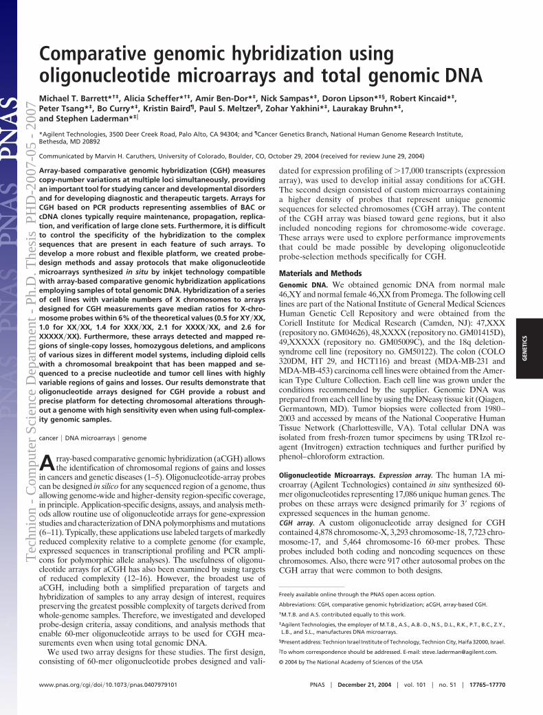
Comparative genomic hybridization usingoligonucleotide microarrays and total genomic DNAMichael T. Barrett*†‡, Alicia Scheffer*†‡, Amir Ben-Dor*‡, Nick Sampas*‡, Doron Lipson*‡§, Robert Kincaid*‡,Peter Tsang*‡, Bo Curry*‡, Kristin Baird¶, Paul S. Meltzer¶, Zohar Yakhini*‡, Laurakay Bruhn*‡,and Stephen Laderman*‡�
*Agilent Technologies, 3500 Deer Creek Road, Palo Alto, CA 94304; and ¶Cancer Genetics Branch, National Human Genome Research Institute,Bethesda, MD 20892
Communicated by Marvin H. Caruthers, University of Colorado, Boulder, CO, October 29, 2004 (received for review June 29, 2004)
Array-based comparative genomic hybridization (CGH) measurescopy-number variations at multiple loci simultaneously, providingan important tool for studying cancer and developmental disordersand for developing diagnostic and therapeutic targets. Arrays forCGH based on PCR products representing assemblies of BAC orcDNA clones typically require maintenance, propagation, replica-tion, and verification of large clone sets. Furthermore, it is difficultto control the specificity of the hybridization to the complexsequences that are present in each feature of such arrays. Todevelop a more robust and flexible platform, we created probe-design methods and assay protocols that make oligonucleotidemicroarrays synthesized in situ by inkjet technology compatiblewith array-based comparative genomic hybridization applicationsemploying samples of total genomic DNA. Hybridization of a seriesof cell lines with variable numbers of X chromosomes to arraysdesigned for CGH measurements gave median ratios for X-chro-mosome probes within 6% of the theoretical values (0.5 for XY�XX,1.0 for XX�XX, 1.4 for XXX�XX, 2.1 for XXXX�XX, and 2.6 forXXXXX�XX). Furthermore, these arrays detected and mapped re-gions of single-copy losses, homozygous deletions, and ampliconsof various sizes in different model systems, including diploid cellswith a chromosomal breakpoint that has been mapped and se-quenced to a precise nucleotide and tumor cell lines with highlyvariable regions of gains and losses. Our results demonstrate thatoligonucleotide arrays designed for CGH provide a robust andprecise platform for detecting chromosomal alterations through-out a genome with high sensitivity even when using full-complex-ity genomic samples.
cancer � DNA microarrays � genome
Array-based comparative genomic hybridization (aCGH) allowsthe identification of chromosomal regions of gains and losses
in cancers and genetic diseases (1–5). Oligonucleotide-array probescan be designed in silico for any sequenced region of a genome, thusallowing genome-wide and higher-density region-specific coverage,in principle. Application-specific designs, assays, and analysis meth-ods allow routine use of oligonucleotide arrays for gene-expressionstudies and characterization of DNA polymorphisms and mutations(6–11). Typically, these applications use labeled targets of markedlyreduced complexity relative to a complete genome (for example,expressed sequences in transcriptional profiling and PCR ampli-cons for polymorphic allele analyses). The usefulness of oligonu-cleotide arrays for aCGH has also been examined by using targetsof reduced complexity (12–16). However, the broadest use ofaCGH, including both a simplified preparation of targets andhybridization of samples to any array design of interest, requirespreserving the greatest possible complexity of targets derived fromwhole-genome samples. Therefore, we investigated and developedprobe-design criteria, assay conditions, and analysis methods thatenable 60-mer oligonucleotide arrays to be used for CGH mea-surements even when using total genomic DNA.
We used two array designs for these studies. The first design,consisting of 60-mer oligonucleotide probes designed and vali-
dated for expression profiling of �17,000 transcripts (expressionarray), was used to develop initial assay conditions for aCGH.The second design consisted of custom microarrays containinga higher density of probes that represent unique genomicsequences for selected chromosomes (CGH array). The contentof the CGH array was biased toward gene regions, but it alsoincluded noncoding regions for chromosome-wide coverage.These arrays were used to explore performance improvementsthat could be made possible by developing oligonucleotideprobe-selection methods specifically for CGH.
Materials and MethodsGenomic DNA. We obtained genomic DNA from normal male46,XY and normal female 46,XX from Promega. The following celllines are part of the National Institute of General Medical SciencesHuman Genetic Cell Repository and were obtained from theCoriell Institute for Medical Research (Camden, NJ): 47,XXX(repository no. GM04626), 48,XXXX (repository no. GM01415D),49,XXXXX (repository no. GM05009C), and the 18q deletion-syndrome cell line (repository no. GM50122). The colon (COLO320DM, HT 29, and HCT116) and breast (MDA-MB-231 andMDA-MB-453) carcinoma cell lines were obtained from the Amer-ican Type Culture Collection. Each cell line was grown under theconditions recommended by the supplier. Genomic DNA wasprepared from each cell line by using the DNeasy tissue kit (Qiagen,Germantown, MD). Tumor biopsies were collected from 1980–2003 and accessed by means of the National Cooperative HumanTissue Network (Charlottesville, VA). Total cellular DNA wasisolated from fresh-frozen tumor specimens by using TRIzol re-agent (Invitrogen) extraction techniques and further purified byphenol–chloroform extraction.
Oligonucleotide Microarrays. Expression array. The human 1A mi-croarray (Agilent Technologies) contained in situ synthesized 60-mer oligonucleotides representing 17,086 unique human genes. Theprobes on these arrays were designed primarily for 3� regions ofexpressed sequences in the human genome.CGH array. A custom oligonucleotide array designed for CGHcontained 4,878 chromosome-X, 3,293 chromosome-18, 7,723 chro-mosome-17, and 5,464 chromosome-16 60-mer probes. Theseprobes included both coding and noncoding sequences on thesechromosomes. Also, there were 917 other autosomal probes on theCGH array that were common to both designs.
Freely available online through the PNAS open access option.
Abbreviations: CGH, comparative genomic hybridization; aCGH, array-based CGH.
†M.T.B. and A.S. contributed equally to this work.
‡Agilent Technologies, the employer of M.T.B., A.S., A.B.-D., N.S., D.L., R.K., P.T., B.C., Z.Y.,L.B., and S.L., manufactures DNA microarrays.
§Present address: Technion Israel Institute of Technology, Technion City, Haifa 32000, Israel.
�To whom correspondence should be addressed. E-mail: steve�[email protected].
© 2004 by The National Academy of Sciences of the USA
www.pnas.org�cgi�doi�10.1073�pnas.0407979101 PNAS � December 21, 2004 � vol. 101 � no. 51 � 17765–17770
GEN
ETIC
S
Tec
hnio
n -
Com
pute
r Sc
ienc
e D
epar
tmen
t - P
h.D
. The
sis
PH
D-2
007-
05 -
200
7
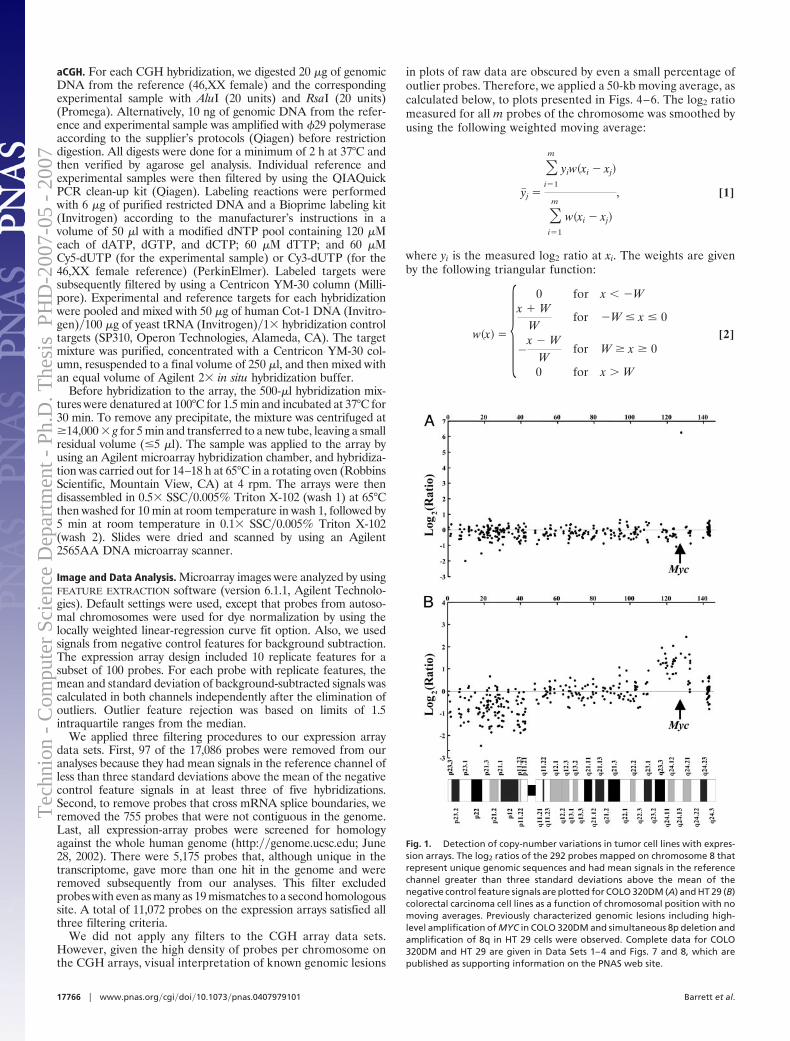
aCGH. For each CGH hybridization, we digested 20 �g of genomicDNA from the reference (46,XX female) and the correspondingexperimental sample with AluI (20 units) and RsaI (20 units)(Promega). Alternatively, 10 ng of genomic DNA from the refer-ence and experimental sample was amplified with �29 polymeraseaccording to the supplier’s protocols (Qiagen) before restrictiondigestion. All digests were done for a minimum of 2 h at 37°C andthen verified by agarose gel analysis. Individual reference andexperimental samples were then filtered by using the QIAQuickPCR clean-up kit (Qiagen). Labeling reactions were performedwith 6 �g of purified restricted DNA and a Bioprime labeling kit(Invitrogen) according to the manufacturer’s instructions in avolume of 50 �l with a modified dNTP pool containing 120 ��each of dATP, dGTP, and dCTP; 60 �� dTTP; and 60 ��Cy5-dUTP (for the experimental sample) or Cy3-dUTP (for the46,XX female reference) (PerkinElmer). Labeled targets weresubsequently filtered by using a Centricon YM-30 column (Milli-pore). Experimental and reference targets for each hybridizationwere pooled and mixed with 50 �g of human Cot-1 DNA (Invitro-gen)�100 �g of yeast tRNA (Invitrogen)�1� hybridization controltargets (SP310, Operon Technologies, Alameda, CA). The targetmixture was purified, concentrated with a Centricon YM-30 col-umn, resuspended to a final volume of 250 �l, and then mixed withan equal volume of Agilent 2� in situ hybridization buffer.
Before hybridization to the array, the 500-�l hybridization mix-tures were denatured at 100°C for 1.5 min and incubated at 37°C for30 min. To remove any precipitate, the mixture was centrifuged at�14,000 � g for 5 min and transferred to a new tube, leaving a smallresidual volume (�5 �l). The sample was applied to the array byusing an Agilent microarray hybridization chamber, and hybridiza-tion was carried out for 14–18 h at 65°C in a rotating oven (RobbinsScientific, Mountain View, CA) at 4 rpm. The arrays were thendisassembled in 0.5� SSC�0.005% Triton X-102 (wash 1) at 65°Cthen washed for 10 min at room temperature in wash 1, followed by5 min at room temperature in 0.1� SSC�0.005% Triton X-102(wash 2). Slides were dried and scanned by using an Agilent2565AA DNA microarray scanner.
Image and Data Analysis. Microarray images were analyzed by usingFEATURE EXTRACTION software (version 6.1.1, Agilent Technolo-gies). Default settings were used, except that probes from autoso-mal chromosomes were used for dye normalization by using thelocally weighted linear-regression curve fit option. Also, we usedsignals from negative control features for background subtraction.The expression array design included 10 replicate features for asubset of 100 probes. For each probe with replicate features, themean and standard deviation of background-subtracted signals wascalculated in both channels independently after the elimination ofoutliers. Outlier feature rejection was based on limits of 1.5intraquartile ranges from the median.
We applied three filtering procedures to our expression arraydata sets. First, 97 of the 17,086 probes were removed from ouranalyses because they had mean signals in the reference channel ofless than three standard deviations above the mean of the negativecontrol feature signals in at least three of five hybridizations.Second, to remove probes that cross mRNA splice boundaries, weremoved the 755 probes that were not contiguous in the genome.Last, all expression-array probes were screened for homologyagainst the whole human genome (http:��genome.ucsc.edu; June28, 2002). There were 5,175 probes that, although unique in thetranscriptome, gave more than one hit in the genome and wereremoved subsequently from our analyses. This filter excludedprobes with even as many as 19 mismatches to a second homologoussite. A total of 11,072 probes on the expression arrays satisfied allthree filtering criteria.
We did not apply any filters to the CGH array data sets.However, given the high density of probes per chromosome onthe CGH arrays, visual interpretation of known genomic lesions
in plots of raw data are obscured by even a small percentage ofoutlier probes. Therefore, we applied a 50-kb moving average, ascalculated below, to plots presented in Figs. 4–6. The log2 ratiomeasured for all m probes of the chromosome was smoothed byusing the following weighted moving average:
y�j �
�i�1
m
yiw�xi � xj�
�i�1
m
w�xi � xj�
, [1]
where yi is the measured log2 ratio at xi. The weights are givenby the following triangular function:
w�x� � �0 for x � �W
x � WW
for �W � x � 0
�x � W
Wfor W � x � 0
0 for x W
[2]
Fig. 1. Detection of copy-number variations in tumor cell lines with expres-sion arrays. The log2 ratios of the 292 probes mapped on chromosome 8 thatrepresent unique genomic sequences and had mean signals in the referencechannel greater than three standard deviations above the mean of thenegative control feature signals are plotted for COLO 320DM (A) and HT 29 (B)colorectal carcinoma cell lines as a function of chromosomal position with nomoving averages. Previously characterized genomic lesions including high-level amplification of MYC in COLO 320DM and simultaneous 8p deletion andamplification of 8q in HT 29 cells were observed. Complete data for COLO320DM and HT 29 are given in Data Sets 1–4 and Figs. 7 and 8, which arepublished as supporting information on the PNAS web site.
17766 � www.pnas.org�cgi�doi�10.1073�pnas.0407979101 Barrett et al.
Tec
hnio
n -
Com
pute
r Sc
ienc
e D
epar
tmen
t - P
h.D
. The
sis
PH
D-2
007-
05 -
200
7
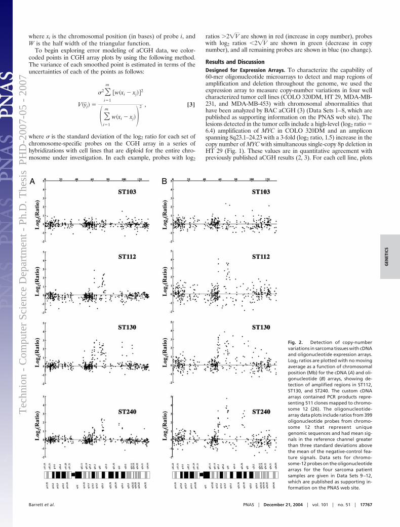
where xi is the chromosomal position (in bases) of probe i, andW is the half width of the triangular function.
To begin exploring error modeling of aCGH data, we color-coded points in CGH array plots by using the following method.The variance of each smoothed point is estimated in terms of theuncertainties of each of the points as follows:
V�y�j� �
2�i�1
m
w�xi � xj�2
��i�1
m
w�xi � xj��2 , [3]
where is the standard deviation of the log2 ratio for each set ofchromosome-specific probes on the CGH array in a series ofhybridizations with cell lines that are diploid for the entire chro-mosome under investigation. In each example, probes with log2
ratios �2�V are shown in red (increase in copy number), probeswith log2 ratios �2�V are shown in green (decrease in copynumber), and all remaining probes are shown in blue (no change).
Results and DiscussionDesigned for Expression Arrays. To characterize the capability of60-mer oligonucleotide microarrays to detect and map regions ofamplification and deletion throughout the genome, we used theexpression array to measure copy-number variations in four wellcharacterized tumor cell lines (COLO 320DM, HT 29, MDA-MB-231, and MDA-MB-453) with chromosomal abnormalities thathave been analyzed by BAC aCGH (3) (Data Sets 1–8, which arepublished as supporting information on the PNAS web site). Thelesions detected in the tumor cells include a high-level (log2 ratio �6.4) amplification of MYC in COLO 320DM and an ampliconspanning 8q23.1–24.23 with a 3-fold (log2 ratio, 1.5) increase in thecopy number of MYC with simultaneous single-copy 8p deletion inHT 29 (Fig. 1). These values are in quantitative agreement withpreviously published aCGH results (2, 3). For each cell line, plots
Fig. 2. Detection of copy-numbervariations in sarcoma tissues with cDNAand oligonucleotide expression arrays.Log2 ratios are plotted with no movingaverage as a function of chromosomalposition (Mb) for the cDNA (A) and oli-gonucleotide (B) arrays, showing de-tection of amplified regions in ST112,ST130, and ST240. The custom cDNAarrays contained PCR products repre-senting 511 clones mapped to chromo-some 12 (26). The oligonucleotide-array data plots include ratios from 399oligonucleotide probes from chromo-some 12 that represent uniquegenomic sequences and had mean sig-nals in the reference channel greaterthan three standard deviations abovethe mean of the negative-control fea-ture signals. Data sets for chromo-some-12 probes on the oligonucleotidearrays for the four sarcoma patientsamples are given in Data Sets 9–12,which are published as supporting in-formation on the PNAS web site.
Barrett et al. PNAS � December 21, 2004 � vol. 101 � no. 51 � 17767
GEN
ETIC
S
Tec
hnio
n -
Com
pute
r Sc
ienc
e D
epar
tmen
t - P
h.D
. The
sis
PH
D-2
007-
05 -
200
7
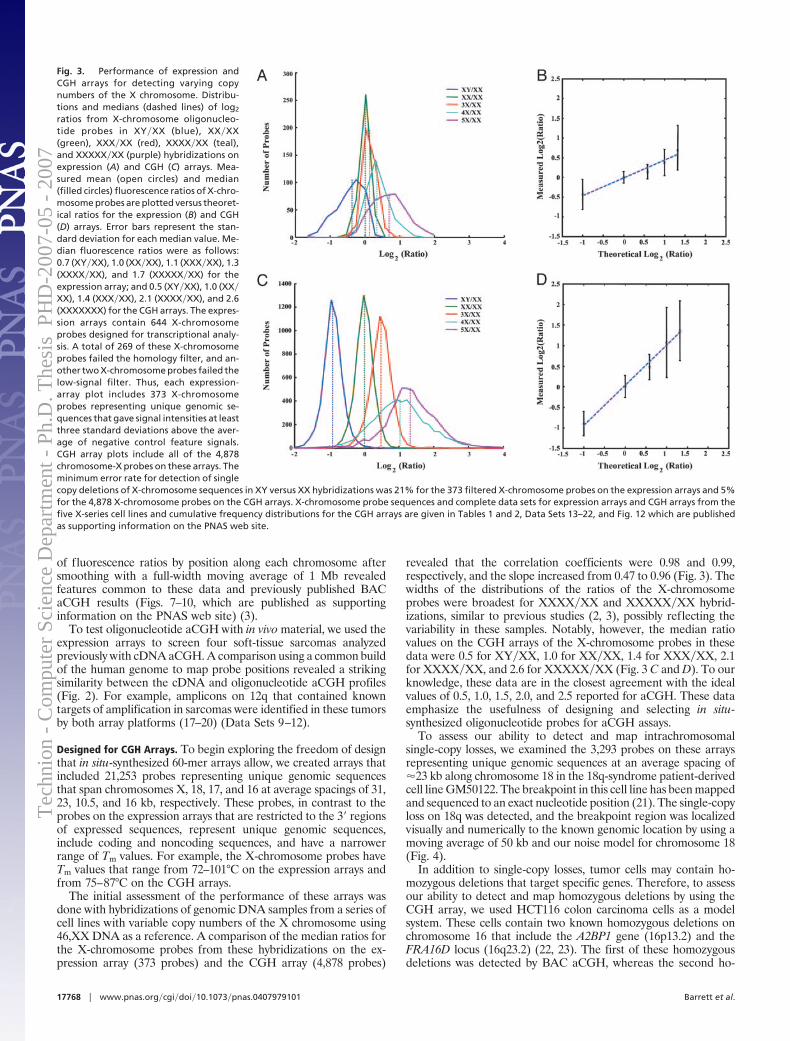
of fluorescence ratios by position along each chromosome aftersmoothing with a full-width moving average of 1 Mb revealedfeatures common to these data and previously published BACaCGH results (Figs. 7–10, which are published as supportinginformation on the PNAS web site) (3).
To test oligonucleotide aCGH with in vivo material, we used theexpression arrays to screen four soft-tissue sarcomas analyzedpreviously with cDNA aCGH. A comparison using a common buildof the human genome to map probe positions revealed a strikingsimilarity between the cDNA and oligonucleotide aCGH profiles(Fig. 2). For example, amplicons on 12q that contained knowntargets of amplification in sarcomas were identified in these tumorsby both array platforms (17–20) (Data Sets 9–12).
Designed for CGH Arrays. To begin exploring the freedom of designthat in situ-synthesized 60-mer arrays allow, we created arrays thatincluded 21,253 probes representing unique genomic sequencesthat span chromosomes X, 18, 17, and 16 at average spacings of 31,23, 10.5, and 16 kb, respectively. These probes, in contrast to theprobes on the expression arrays that are restricted to the 3� regionsof expressed sequences, represent unique genomic sequences,include coding and noncoding sequences, and have a narrowerrange of Tm values. For example, the X-chromosome probes haveTm values that range from 72–101°C on the expression arrays andfrom 75–87°C on the CGH arrays.
The initial assessment of the performance of these arrays wasdone with hybridizations of genomic DNA samples from a series ofcell lines with variable copy numbers of the X chromosome using46,XX DNA as a reference. A comparison of the median ratios forthe X-chromosome probes from these hybridizations on the ex-pression array (373 probes) and the CGH array (4,878 probes)
revealed that the correlation coefficients were 0.98 and 0.99,respectively, and the slope increased from 0.47 to 0.96 (Fig. 3). Thewidths of the distributions of the ratios of the X-chromosomeprobes were broadest for XXXX�XX and XXXXX�XX hybrid-izations, similar to previous studies (2, 3), possibly reflecting thevariability in these samples. Notably, however, the median ratiovalues on the CGH arrays of the X-chromosome probes in thesedata were 0.5 for XY�XX, 1.0 for XX�XX, 1.4 for XXX�XX, 2.1for XXXX�XX, and 2.6 for XXXXX�XX (Fig. 3 C and D). To ourknowledge, these data are in the closest agreement with the idealvalues of 0.5, 1.0, 1.5, 2.0, and 2.5 reported for aCGH. These dataemphasize the usefulness of designing and selecting in situ-synthesized oligonucleotide probes for aCGH assays.
To assess our ability to detect and map intrachromosomalsingle-copy losses, we examined the 3,293 probes on these arraysrepresenting unique genomic sequences at an average spacing of 23 kb along chromosome 18 in the 18q-syndrome patient-derivedcell line GM50122. The breakpoint in this cell line has been mappedand sequenced to an exact nucleotide position (21). The single-copyloss on 18q was detected, and the breakpoint region was localizedvisually and numerically to the known genomic location by using amoving average of 50 kb and our noise model for chromosome 18(Fig. 4).
In addition to single-copy losses, tumor cells may contain ho-mozygous deletions that target specific genes. Therefore, to assessour ability to detect and map homozygous deletions by using theCGH array, we used HCT116 colon carcinoma cells as a modelsystem. These cells contain two known homozygous deletions onchromosome 16 that include the A2BP1 gene (16p13.2) and theFRA16D locus (16q23.2) (22, 23). The first of these homozygousdeletions was detected by BAC aCGH, whereas the second ho-
Fig. 3. Performance of expression andCGH arrays for detecting varying copynumbers of the X chromosome. Distribu-tions and medians (dashed lines) of log2
ratios from X-chromosome oligonucleo-tide probes in XY�XX (blue), XX�XX(green), XXX�XX (red), XXXX�XX (teal),and XXXXX�XX (purple) hybridizations onexpression (A) and CGH (C) arrays. Mea-sured mean (open circles) and median(filled circles) fluorescence ratios of X-chro-mosome probes are plotted versus theoret-ical ratios for the expression (B) and CGH(D) arrays. Error bars represent the stan-dard deviation for each median value. Me-dian fluorescence ratios were as follows:0.7 (XY�XX), 1.0 (XX�XX), 1.1 (XXX�XX), 1.3(XXXX�XX), and 1.7 (XXXXX�XX) for theexpression array; and 0.5 (XY�XX), 1.0 (XX�XX), 1.4 (XXX�XX), 2.1 (XXXX�XX), and 2.6(XXXXXXX) for the CGH arrays. The expres-sion arrays contain 644 X-chromosomeprobes designed for transcriptional analy-sis. A total of 269 of these X-chromosomeprobes failed the homology filter, and an-other two X-chromosome probes failed thelow-signal filter. Thus, each expression-array plot includes 373 X-chromosomeprobes representing unique genomic se-quences that gave signal intensities at leastthree standard deviations above the aver-age of negative control feature signals.CGH array plots include all of the 4,878chromosome-X probes on these arrays. Theminimum error rate for detection of singlecopy deletions of X-chromosome sequences in XY versus XX hybridizations was 21% for the 373 filtered X-chromosome probes on the expression arrays and 5%for the 4,878 X-chromosome probes on the CGH arrays. X-chromosome probe sequences and complete data sets for expression arrays and CGH arrays from thefive X-series cell lines and cumulative frequency distributions for the CGH arrays are given in Tables 1 and 2, Data Sets 13–22, and Fig. 12 which are publishedas supporting information on the PNAS web site.
17768 � www.pnas.org�cgi�doi�10.1073�pnas.0407979101 Barrett et al.
Tec
hnio
n -
Com
pute
r Sc
ienc
e D
epar
tmen
t - P
h.D
. The
sis
PH
D-2
007-
05 -
200
7
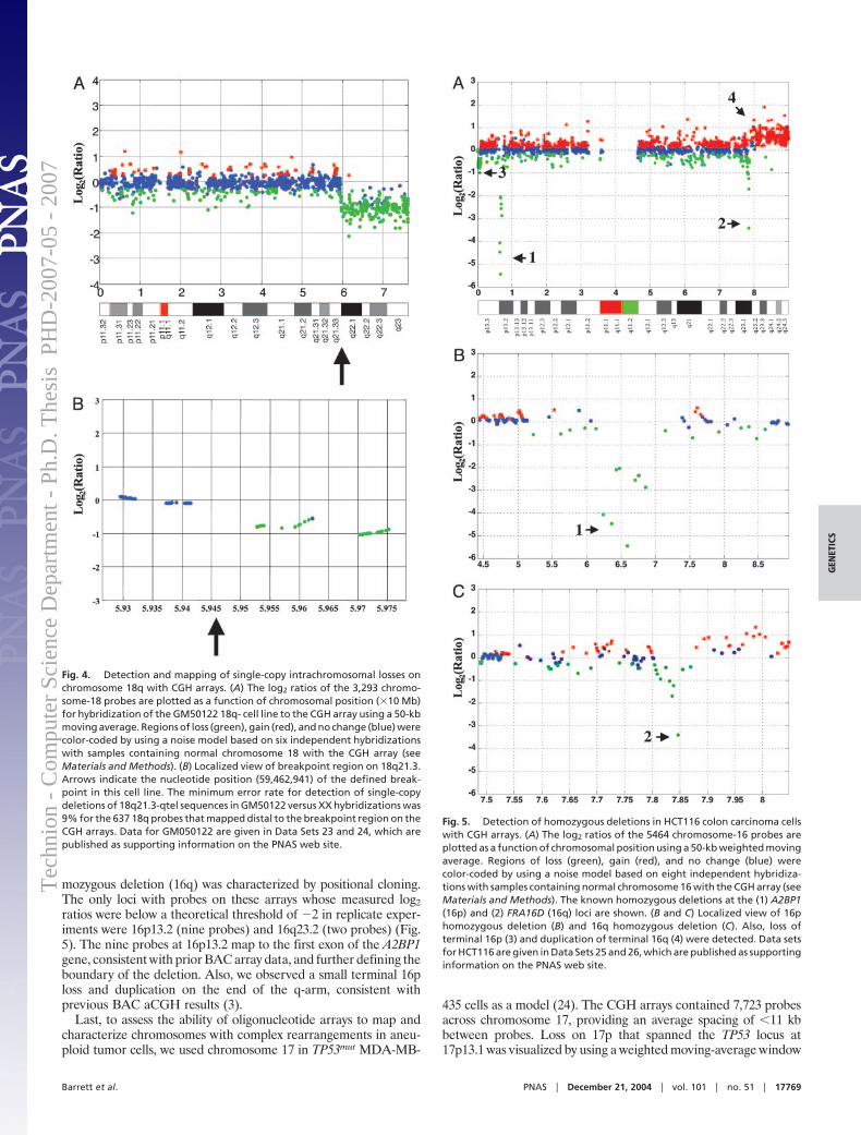
mozygous deletion (16q) was characterized by positional cloning.The only loci with probes on these arrays whose measured log2ratios were below a theoretical threshold of �2 in replicate exper-iments were 16p13.2 (nine probes) and 16q23.2 (two probes) (Fig.5). The nine probes at 16p13.2 map to the first exon of the A2BP1gene, consistent with prior BAC array data, and further defining theboundary of the deletion. Also, we observed a small terminal 16ploss and duplication on the end of the q-arm, consistent withprevious BAC aCGH results (3).
Last, to assess the ability of oligonucleotide arrays to map andcharacterize chromosomes with complex rearrangements in aneu-ploid tumor cells, we used chromosome 17 in TP53mut MDA-MB-
435 cells as a model (24). The CGH arrays contained 7,723 probesacross chromosome 17, providing an average spacing of �11 kbbetween probes. Loss on 17p that spanned the TP53 locus at17p13.1 was visualized by using a weighted moving-average window
Fig. 4. Detection and mapping of single-copy intrachromosomal losses onchromosome 18q with CGH arrays. (A) The log2 ratios of the 3,293 chromo-some-18 probes are plotted as a function of chromosomal position (�10 Mb)for hybridization of the GM50122 18q- cell line to the CGH array using a 50-kbmoving average. Regions of loss (green), gain (red), and no change (blue) werecolor-coded by using a noise model based on six independent hybridizationswith samples containing normal chromosome 18 with the CGH array (seeMaterials and Methods). (B) Localized view of breakpoint region on 18q21.3.Arrows indicate the nucleotide position (59,462,941) of the defined break-point in this cell line. The minimum error rate for detection of single-copydeletions of 18q21.3-qtel sequences in GM50122 versus XX hybridizations was9% for the 637 18q probes that mapped distal to the breakpoint region on theCGH arrays. Data for GM050122 are given in Data Sets 23 and 24, which arepublished as supporting information on the PNAS web site.
Fig. 5. Detection of homozygous deletions in HCT116 colon carcinoma cellswith CGH arrays. (A) The log2 ratios of the 5464 chromosome-16 probes areplotted as a function of chromosomal position using a 50-kb weighted movingaverage. Regions of loss (green), gain (red), and no change (blue) werecolor-coded by using a noise model based on eight independent hybridiza-tions with samples containing normal chromosome 16 with the CGH array (seeMaterials and Methods). The known homozygous deletions at the (1) A2BP1(16p) and (2) FRA16D (16q) loci are shown. (B and C) Localized view of 16phomozygous deletion (B) and 16q homozygous deletion (C). Also, loss ofterminal 16p (3) and duplication of terminal 16q (4) were detected. Data setsfor HCT116 are given in Data Sets 25 and 26, which are published as supportinginformation on the PNAS web site.
Barrett et al. PNAS � December 21, 2004 � vol. 101 � no. 51 � 17769
GEN
ETIC
S
Tec
hnio
n -
Com
pute
r Sc
ienc
e D
epar
tmen
t - P
h.D
. The
sis
PH
D-2
007-
05 -
200
7

of 50 kb (Fig. 6). Also, distinct regions of gain (e.g., q21.32-q21.33,q23.2-q24.3, q25.1, and q25.3) and loss (e.g., 17q21.2-q21.31, q23.2,and q24.3) were detected with these arrays, consistent with previ-ously published aCGH data (3). Recent studies have shown thathighly processive DNA polymerases, such as �29, can be used toprepare templates from limiting starting materials for aCGHmeasurements (25). The same patterns of chromosome 17 lossesand gains in MDA-MB-453 cells were detected with the CGHarrays by using 10 ng of starting material and �29 amplification (Fig.11, which is published as supporting information on the PNAS website).
Our results demonstrate that in situ synthesized 60-mer oli-gonucleotide arrays can reproducibly detect genomic lesionsincluding single-copy and homozygous deletions, as well asvariable amplicons even when using whole genomes as targets.
Also, we show that our initial design and selection of oligonu-cleotide probes for CGH measurements enable more accuratemeasurements of genomic DNA copy-number changes than60-mer probes optimized for mRNA detection. These findingsimply that additional theoretical and experimental efforts torefine probe sequence selection, assay protocols, and analysismethods may yield further improvements in performance. Theability to use full-complexity samples with oligonucleotide arraysprovides researchers the flexibility and performance to studycopy-number variation in essentially any region of the genomewith a single, simplified sample preparation. Thus, our datasuggest that this technology could emerge as a standard tool forresearch and diagnostics of cancer and genetic disease.
We thank Michael Bittner for critical reading of the manuscript.
1. Pinkel, D., Segraves, R., Sudar, D., Clark, S., Poole, I., Kowbel, D., Collins, C., Kuo,W. L., Chen, C., Zhai, Y., et al. (1998) Nat. Genet. 20, 207–211.
2. Pollack, J. R., Perou, C. M., Alizadeh, A. A., Eisen, M. B., Pergamenschikov, A.,Williams, C. F., Jeffrey, S. S., Botstein, D. & Brown, P. O. (1999) Nat. Genet. 23,41–46.
3. Snijders, A. M., Nowak, N., Segraves, R., Blackwood, S., Brown, N., Conroy, J.,Hamilton, G., Hindle, A. K., Huey, B., Kimura, K., et al. (2001) Nat. Genet. 29,263–264.
4. Greshock, J., Naylor, T. L., Margolin, A., Diskin, S., Cleaver, S. H., Futreal, P. A.,deJong, P. J., Zhao, S., Liebman, M. & Weber, B. L. (2004) Genome Res. 14, 179–187.
5. Hodgson, G., Hager, J. H., Volik, S., Hariono, S., Wernick, M., Moore, D., Nowak,N., Albertson, D. G., Pinkel, D., Collins, C., et al. (2001) Nat. Genet. 29, 459–464.
6. Chee, M., Yang, R., Hubell, E., Berno, A., Huang, X., Stern, D., Winkler, J.,Lockhart, D., Morris, M. & Fodor, S. (1996) Science 274, 610–614.
7. Lockhart, D., Dong, H., Byrne, M., Follettie, M., Gallo, M., Chee, M., Mittmann, M.,Wang, C., Kobayashi, M., Horton, H. & Brown, E. (1996) Nat. Biotechnol. 14,1675–1680.
8. Hughes, T. R., Mao, M., Jones, A. R., Burchard, J., Marton, M. J., Shannon, K. W.,Lefkowitz, S. M., Ziman, M., Schelter, J. M., Meyer, M. R., et al. (2001) Nat.Biotechnol. 19, 342–347.
9. Hacia, J., Brody, L., Chee, M., Fodor, S. & Collins, F. (1996) Nat. Genet. 14, 441–447.10. Lindblad-Toh, K., Tanenbaum, D. M., Daly, M. J., Winchester, E., Lui, W. O.,
Villapakkam, A., Stanton, S. E., Larsson, C., Hudson, T. J., Johnson, B. E., et al.(2000) Nat. Biotechnol. 18, 1001–1005.
11. Kennedy, G. C., Matsuzaki, H., Dong, S., Liu, W. M., Huang, J., Liu, G., Su, X., Cao,M., Chen, W., Zhang, J., et al. (2003) Nat. Biotechnol. 21, 1233–1237.
12. Gray, J. W., Pinkel, D., Albertson, D., Collins, C. & Baldocchi, R. (1999) U.S. PatentUS6465182.
13. Wigler, M. & Lucito, R. (1998) U.S. Patent US9823168.
14. Lucito, R., Healy, J., Alexander, J., Reiner, A., Esposito, D., Chi, M., Rodgers, L.,Brady, A., Sebat, J., Troge, J., et al. (2003) Genome Res. 13, 2291–2305.
15. Zhao, X., Li, C., Paez, J. G., Chin, K., Janne, P. A., Chen, T. H., Girard, L., Minna,J., Christiani, D., Leo, C., et al. (2004) Cancer Res. 64, 3060–3071.
16. Bignell, G. R., Huang, J., Greshock, J., Watt, S., Butler, A., West, S., Grigorova, M.,Jones, K. W., Wei, W., Stratton, M. R., et al. (2004) Genome Res. 14, 287–295.
17. Jankowski, S. A., Mitchell, D. S., Smith, S. H., Trent, J. M. & Meltzer, P. S. (1994)Oncogene 9, 1205–1211.
18. Fritz, B., Schubert, F., Wrobel, G., Schwaenen, C., Wessendorf, S., Nessling, M.,Korz, C., Rieker, R. J., Montgomery, K., Kucherlapati, R., et al. (2002) Cancer Res.62, 2993–2998.
19. Reifenberger, G., Ichimura, K., Reifenberger, J., Elkahloun, A. G., Meltzer, P. S. &Collins, V. P. (1996) Cancer Res. 56, 5141–5145.
20. Meza-Zepeda, L. A., Berner, J. M., Henriksen, J., South, A. P., Pedeutour, F.,Dahlberg, A. B., Godager, L. H., Nizetic, D., Forus, A. & Myklebost, O. (2001) GenesChromosomes Cancer 31, 264–273.
21. Katz, S. G., Schneider, S. S., Bartuski, A., Trask, B. J., Massa, H., Overhauser, J.,Lalande, M., Lansdorp, P. M. & Silverman, G. A. (1999) Hum. Mol. Genet. 8, 87–92.
22. Paige, J. W., Taylor, K. J., Stewart, A., Sgouros, J. G., Gabra, H., Sellar, G. C., Smyth,J. F., Porteous, D. J. & Watson, J. E. V. (2000) Cancer Res. 60, 1690–1697.
23. Albertson, D. G. & Pinkel, D. (2003) Hum. Mol. Genet. 12, Spec. No. 2, R145–52.24. Gayet, J., Zhou, X. P., Duval, A., Rolland, S., Hoang, J. M., Cottu, P. & Hamelin,
R. (2001) Oncogene 20, 5025–5032.25. Paez, J. G., Lin, M., Beroukhim, R., Lee, J. C., Zhao, X., Richter, D. J., Gabriel,
S., Herman, P., Sasaki, H., Altshuler, D., et al. (2004) Nucleic Acids Res. 32, e71.26. Hedenfalk, I., Ringner, M., Ben-Dor, A., Yakhini, Z., Chen, Y., Chebil, G., Ach, R.,
Loman, N., Olsson, H., Meltzer, P., et al. (2003) Proc. Natl. Acad. Sci. USA 100,2532–2537.
Fig. 6. Detection of complex chromosome-17 rearrangements in MDA-MB-453 cells with CGH arrays. The log2 ratios of the 7,723 chromosome-17 probes areplotted as a function of chromosomal position by using a 50-kb weighted moving average. (A) Regions of loss (green), gain (red), and no change (blue) inMDA-MB-453 cells were color-coded by using a noise model based on eight independent hybridizations of samples containing normal chromosome-17 (seeMaterials and Methods). Loss of 17p that spans the TP53 locus (p13.1) was observed. Also, distinct regions of amplification and loss were detected on the q arm.(B) Representative example of log2 ratios for chromosome-17 probes in a 46,XX self�self hybridization. Complete data sets for MDA-MB-453 and 46,XX self�selfare given in Data Sets 27 and 28, which are published as supporting information on the PNAS web site.
17770 � www.pnas.org�cgi�doi�10.1073�pnas.0407979101 Barrett et al.
Tec
hnio
n -
Com
pute
r Sc
ienc
e D
epar
tmen
t - P
h.D
. The
sis
PH
D-2
007-
05 -
200
7
A.2 Optimization of Probe Coverage for High-
Resolution Oligonucleotide aCGH
Doron Lipson, Zohar Yakhini, and Yonatan Aumann, “Optimization ofProbe Coverage for High-Resolution Oligonucleotide aCGH”. Bioin-formatics, 23(2):e77-e83, 2007.
79
Tec
hnio
n -
Com
pute
r Sc
ienc
e D
epar
tmen
t - P
h.D
. The
sis
PH
D-2
007-
05 -
200
7

80
Tec
hnio
n -
Com
pute
r Sc
ienc
e D
epar
tmen
t - P
h.D
. The
sis
PH
D-2
007-
05 -
200
7
BIOINFORMATICS Vol. 00 no. 00 2006Pages 1–7
Optimization of Probe Coverage for High-ResolutionOligonucleotide aCGHDoron Lipson 1,∗ , Zohar Yakhini 1,2, Yonatan Aumann 3
1Computer Science Department, Technion, Israel, 2Agilent Laboratories, CA, USA,3Computer Science Department, Bar-Ilan University, Israel
ABSTRACTMotivation: The resolution at which genomic alterations canbe mapped by means of oligonucleotide aCGH (array-basedComparative Genomic Hybridization) is limited by two factors: theavailability of high-quality probes for the the target genomic sequenceand the array real-estate. Optimization of the probe selection processis required for arrays that are designed to probe specific genomicregions in very high resolution without compromising probe qualityconstraints.Results: In this paper we describe a well-defined optimizationproblem associated with the problem of probe selection for high-resolution aCGH arrays. We propose the whenever possible ε-coveras a formulation that faithfully captures the requirement of probeselection problem, and provide a fast randomized algorithm thatsolves the optimization problem in O(n log n) time, as well as adeterministic algorithm with the same asymptotic performance. Weapply the method in a typical high-definition array design scenario anddemonstrate its superiority with respect to alternative approaches.Availability: Address requests to the authors.Contact: [email protected]
1 INTRODUCTIONAlterations in DNA copy number are characteristic of many cancertypes and are thought to drive some cancer pathogenesis processes.These alterations include large chromosomal gains and losses aswell as smaller scale amplifications and deletions. Because of theirrole in cancer development, regions of chromosomal instability areuseful for elucidating other components of the process. For example,since genomic instability can trigger the activation of oncogenes andthe silencing of tumor suppressors, mapping regions of commongenomic aberrations has been used to discover cancer related genes.Understanding genome aberrations is important for both the basicunderstanding of cancer and for diagnosis and clinical practice.
Alterations in DNA copy number have been initially measuredusing local fluorescence in situ hybridization-based techniques.These evolved to a genome wide technique called ComparativeGenomic Hybridization (CGH, see [6]), now commonly used forthe identification of chromosomal alterations in cancer [12, 2].In this genome-wide cytogenetic method differentially labeledtumor and normal DNA are co-hybridized to normal metaphases.Ratios between the two labels allow the detection of chromosomalamplifications and deletions of regions that may harbor oncogenesand tumor suppressor genes. Classical CGH has, however, a
∗To whom correspondence should be addressed.
limited resolution (10-20 Mbp). With such low resolution it isimpossible to predict the borders of the chromosomal changesor to identify changes in copy numbers of single genes andsmall genomic regions. In a more advanced method termed arrayCGH (aCGH), tumor and normal DNA are co-hybridized to amicroarray of thousands of BAC, cDNA or oligonucleotide probes[13, 14, 10, 5, 4, 3]. The use of aCGH allows the determinationof changes in DNA copy number of relatively small chromosomalregions. Using oligonucleotides arrays the resolution can, in theory,be finer than single genes.
In fact, when using oligonucleotides the resolution appears tohave no limitation as these can be designed to probe any regionin the genome of interest. In reality the resolution is limited fortwo main reasons. One is the fact that not all genomic locationscan be effectively probed. For example, genomic locations that arenot unique to the genome (genomic repeats) or genomic regionswith extreme GC content limit the design of specific probes.The other limitation is array real-estate – the number of genomicregions that can be probed in one array. Note that for technologyimplementations that use redundant probes this number is muchsmaller than the number of features on the array.
In this work we address the joint optimization of these tworesolution limiting factors. The methods we develop are useful inthe context of designing high-definition arrays. These are arraysdesigned to probe specific genomic regions in very high resolution.For this purpose a dense set of probes is selected for the region ofinterest. We are interested in doing so while maintaining optimalcoverage and without compromising probe quality constraints.Major determinants of probe quality are its expected sensitivity,which is predicted by thermodynamic evaluation of the probe-target complex, and specificity, which is inferred from the extentto which close repeats of the probe can be found in the genome.In previous work [8, 9, 11, 15] probe sensitivity and specificityhave been studied mostly in the context of expression profiling.The background context in CGH is different and so is thethermodynamics but the overall considerations remain valid. Themethods described in the current paper are completely independentfrom those used for assigning quality to candidate probes andcan therefore be applicable to any such assignment, including onederived from experimental data.
Lucito et al [10] describe design criteria that are based on anempirically derived quality assignment only. That is – they chooseto use all probes with a given quality or better without takingany uniformity considerations into account. This approach leads tohaving regions that are more densely probed than others as wellas to coverage discontinuities. When studying a given genomic
c© Oxford University Press 2006. 1
Tec
hnio
n -
Com
pute
r Sc
ienc
e D
epar
tmen
t - P
h.D
. The
sis
PH
D-2
007-
05 -
200
7

Lipson et al
region we are typically not biased to any specific sub-regions andseek to obtain copy number information for all sub-regions. It istherefore best to have a uniform (equi-distant) distribution of probesin the region. This way we best avoid coverage discontinuities andhave comparable information about all sub-regions. However, auniformly distributed set of probes will greatly compromise qualityconsiderations. We may be selecting probes that are highly non-specific, for example. This paper describes methods that assumea given quality threshold above which probes are acceptable andthen optimize the coverage using only these candidate probes andworking with the array real-estate constraints.
The rest of the paper is organized as follows: In Section 2we describe a new score that accounts for probe coverage, andformally define the optimization problem. In Section 3 we describetwo algorithms that efficiently solve the defined problem: a faststochastic algorithm, and a deterministic variant. Finally, inSection 4, we demonstrate the application of our method in abiological scenario, and compare the obtained results with somealternative methods.
2 MATHEMATICAL FORMULATIONIn this section we formally define the optimization problemsassociated with probe selection for aCGH arrays, as discussed inthe Introduction. We believe that such a formal definition is ofindependent interest, as the problem is most commonly stated inill-defined terms.
Two types of parameters are typically considered when evaluatingcandidate probes for a hybridization assay. Sensitivity is a measureof a probe’s ability to strongly interact with its target, and istypically assessed by considering the thermodynamic stability of theprobe-target complex. Specificity is a measure of a probe’s abilityto discriminate between its intended target and other non-specificmolecules it might cross hybridize to, and is typically assessed byconsidering the similarity of the target to the expected molecularbackground (e.g. the entire transcriptome in an expression profilingassay, or the entire genome in a aCGH assay). Methods forpredicting the sensitivity and specificity of candidate probes havebeen extensively studied in the past (see Introduction) and willnot be considered here. Instead, we shall assume we are providedwith a quality parameter q(p), specifying the overall predictedperformance of the probe p.
When designing oligonucleotide probes for aCGH an additionalcriterion should also be taken into consideration – that of coverage.Specifically, when an array is designed for the purpose ofpinpointing genomic breakpoints, an important consideration in thedesign is to minimize the uncertainty at which the breakpoints aremapped, wherever they may be. Thus, probes should somehowuniformly spaced, so as to be not “too far” from the location of anypossible breakpoint.
Accordingly, when designing an aCGH array, we are interestedto in selecting “highest quality” probes, with the “best possible”coverage. In this section we provide formal definitions that capturethe intuitive meaning of these notions.
2.1 Probe QualityLet P be the set of candidate probes. For brevity, we identify eachprobe with its genomic location, thus P ⊂ N. Let q : P → R+
be the quality function associating a quality score with each probe.
Intuitively, we are interested in using the “best possible” probes,i.e. those with the highest quality score. However, the high qualityprobes may not be evenly distributed within the genomic area ofinterest. Thus, choosing the globally best probes may result in poorcoverage of the genome. Hence, rather than using the globallyhighest quality probes, we seek to use the locally best probes.Specifically, for a probe p ∈ P and window size w, we define thew-local quality of p to be the percentile of q(p) within scores in thew window around p. Formally, let Pw be the set of candidate probeswithin the window [p− w/2, p + w/2]. Then
qw(p) =|{p′ ∈ Pw : q(p′) ≤ q(p)}|
|Pw|(1)
We now define the “good probes” to be those with high localquality. Formally, for a window size w and threshold τ ∈ [0, 1], thew-local τ -good probes are all the probes p for which qw(p) ≥ τ .We shall seek to use only probes which are w-local τ -good, for someproper choice of w and τ . We note that it is also possible to optimizefor τ , as explained later.
2.2 Probe CoverageAs mentioned, we are also interested that the probes “cover” thegenomic region of interest with the most granular coverage possible.Specifically, if there is a breakpoint at some point on the genome,we would like to be able to determine its location as preciselyas possible. However, two factors limit the precision that canobtained:
• With a limited number of probes in the array, probes cannot beplaced at each genomic location. Rather, they must be spreadacross the region of interest. In this case, the localization ofgenomic events can only be determined by the pair of flankingprobes. We shall seek that for all genomic locations, the gapbetween this pair of probes is as small as possible.
• Some genomic regions do not contain any candidate probes, oronly probes of poor quality. In such cases, large gaps betweenprobes are inevitable. Any breakpoint occurring within thesegaps can only be localized pair of candidate probe borderingthe gap.
Thus, we seek to choose a set of probes that uniformly cover allgenomic locations – whenever possible, and as close as possibleto the points within the large gaps – otherwise. The followingdefinition captures this intuition:
DEFINITION 2.1. Given a genomic region G = [gbeg, gend], aset of candidate probes P = {p1, . . . , pn} and a parameter ε, asubset C = {pi1 , . . . , pik} is a whenever possible (WP) ε-cover ofG with respect to P if, when setting pi0 = p0 = gbeg and pik+1 =pn+1 = gend, for every two adjacent selected probes pij , pij+1 ∈C (0 ≤ j ≤ k) one of the following holds:
1. pij+1 − pij ≤ ε, or
2. ij+1 = ij + 1 (pij , pij+1 are consecutive candidate probes).
For such a cover C, we say that the resolution of C is ε.
Thus, a WP ε-cover of G guarantees that for any possiblebreakpoint x, it can either be localized to within ε base-pairs, orto within the best resolution that could have been obtained evenif all candidate probes would have been used. We believe that the
2
Tec
hnio
n -
Com
pute
r Sc
ienc
e D
epar
tmen
t - P
h.D
. The
sis
PH
D-2
007-
05 -
200
7
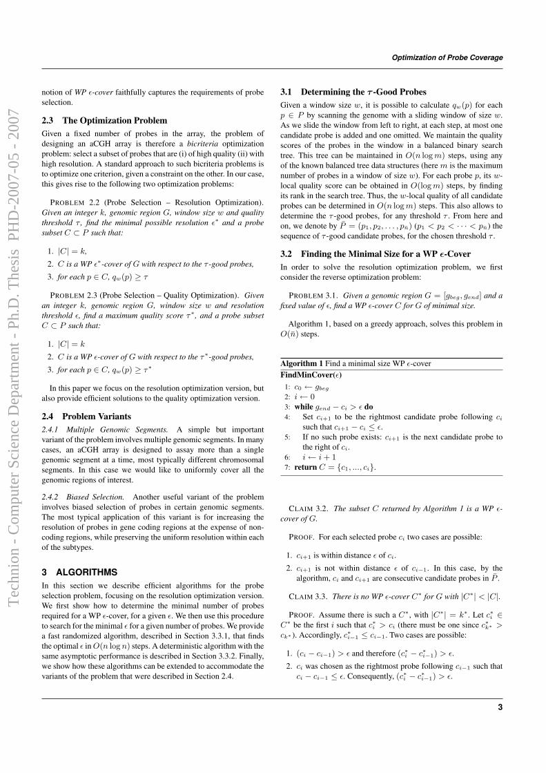
Optimization of Probe Coverage
notion of WP ε-cover faithfully captures the requirements of probeselection.
2.3 The Optimization ProblemGiven a fixed number of probes in the array, the problem ofdesigning an aCGH array is therefore a bicriteria optimizationproblem: select a subset of probes that are (i) of high quality (ii) withhigh resolution. A standard approach to such bicriteria problems isto optimize one criterion, given a constraint on the other. In our case,this gives rise to the following two optimization problems:
PROBLEM 2.2 (Probe Selection – Resolution Optimization).Given an integer k, genomic region G, window size w and qualitythreshold τ , find the minimal possible resolution ε∗ and a probesubset C ⊂ P such that:
1. |C| = k,
2. C is a WP ε∗-cover of G with respect to the τ -good probes,
3. for each p ∈ C, qw(p) ≥ τ
PROBLEM 2.3 (Probe Selection – Quality Optimization). Givenan integer k, genomic region G, window size w and resolutionthreshold ε, find a maximum quality score τ∗, and a probe subsetC ⊂ P such that:
1. |C| = k
2. C is a WP ε-cover of G with respect to the τ∗-good probes,
3. for each p ∈ C, qw(p) ≥ τ∗
In this paper we focus on the resolution optimization version, butalso provide efficient solutions to the quality optimization version.
2.4 Problem Variants2.4.1 Multiple Genomic Segments. A simple but importantvariant of the problem involves multiple genomic segments. In manycases, an aCGH array is designed to assay more than a singlegenomic segment at a time, most typically different chromosomalsegments. In this case we would like to uniformly cover all thegenomic regions of interest.
2.4.2 Biased Selection. Another useful variant of the probleminvolves biased selection of probes in certain genomic segments.The most typical application of this variant is for increasing theresolution of probes in gene coding regions at the expense of non-coding regions, while preserving the uniform resolution within eachof the subtypes.
3 ALGORITHMSIn this section we describe efficient algorithms for the probeselection problem, focusing on the resolution optimization version.We first show how to determine the minimal number of probesrequired for a WP ε-cover, for a given ε. We then use this procedureto search for the minimal ε for a given number of probes. We providea fast randomized algorithm, described in Section 3.3.1, that findsthe optimal ε in O(n log n) steps. A deterministic algorithm with thesame asymptotic performance is described in Section 3.3.2. Finally,we show how these algorithms can be extended to accommodate thevariants of the problem that were described in Section 2.4.
3.1 Determining the τ -Good ProbesGiven a window size w, it is possible to calculate qw(p) for eachp ∈ P by scanning the genome with a sliding window of size w.As we slide the window from left to right, at each step, at most onecandidate probe is added and one omitted. We maintain the qualityscores of the probes in the window in a balanced binary searchtree. This tree can be maintained in O(n log m) steps, using anyof the known balanced tree data structures (here m is the maximumnumber of probes in a window of size w). For each probe p, its w-local quality score can be obtained in O(log m) steps, by findingits rank in the search tree. Thus, the w-local quality of all candidateprobes can be determined in O(n log m) steps. This also allows todetermine the τ -good probes, for any threshold τ . From here andon, we denote by P = (p1, p2, . . . , pn) (p1 < p2 < · · · < pn) thesequence of τ -good candidate probes, for the chosen threshold τ .
3.2 Finding the Minimal Size for a WP ε-CoverIn order to solve the resolution optimization problem, we firstconsider the reverse optimization problem:
PROBLEM 3.1. Given a genomic region G = [gbeg, gend] and afixed value of ε, find a WP ε-cover C for G of minimal size.
Algorithm 1, based on a greedy approach, solves this problem inO(n) steps.
Algorithm 1 Find a minimal size WP ε-coverFindMinCover(ε)
1: c0 ← gbeg
2: i← 03: while gend − ci > ε do4: Set ci+1 to be the rightmost candidate probe following ci
such that ci+1 − ci ≤ ε.5: If no such probe exists: ci+1 is the next candidate probe to
the right of ci.6: i← i + 17: return C = {c1, ..., ci}.
CLAIM 3.2. The subset C returned by Algorithm 1 is a WP ε-cover of G.
PROOF. For each selected probe ci two cases are possible:
1. ci+1 is within distance ε of ci.
2. ci+1 is not within distance ε of ci−1. In this case, by thealgorithm, ci and ci+1 are consecutive candidate probes in P .
CLAIM 3.3. There is no WP ε-cover C∗ for G with |C∗| < |C|.
PROOF. Assume there is such a C∗, with |C∗| = k∗. Let c∗i ∈C∗ be the first i such that c∗i > ci (there must be one since c∗k∗ >ck∗ ). Accordingly, c∗i−1 ≤ ci−1. Two cases are possible:
1. (ci − ci−1) > ε and therefore (c∗i − c∗i−1) > ε.
2. ci was chosen as the rightmost probe following ci−1 such thatci − ci−1 ≤ ε. Consequently, (c∗i − c∗i−1) > ε.
3
Tec
hnio
n -
Com
pute
r Sc
ienc
e D
epar
tmen
t - P
h.D
. The
sis
PH
D-2
007-
05 -
200
7
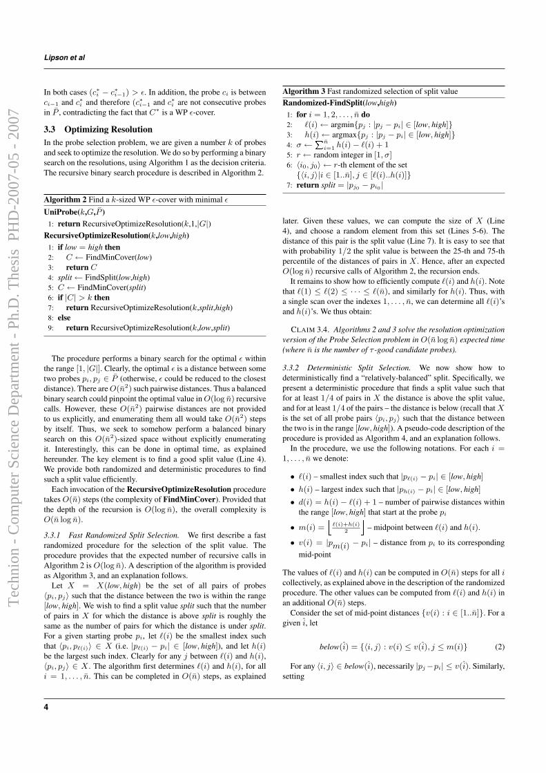
Lipson et al
In both cases (c∗i − c∗i−1) > ε. In addition, the probe ci is betweenci−1 and c∗i and therefore (c∗i−1 and c∗i are not consecutive probesin P , contradicting the fact that C∗ is a WP ε-cover.
3.3 Optimizing ResolutionIn the probe selection problem, we are given a number k of probesand seek to optimize the resolution. We do so by performing a binarysearch on the resolutions, using Algorithm 1 as the decision criteria.The recursive binary search procedure is described in Algorithm 2.
Algorithm 2 Find a k-sized WP ε-cover with minimal ε
UniProbe(k,G,P )1: return RecursiveOptimizeResolution(k,1,|G|)
RecursiveOptimizeResolution(k,low,high)1: if low = high then2: C ← FindMinCover(low)3: return C4: split← FindSplit(low,high)5: C ← FindMinCover(split)6: if |C| > k then7: return RecursiveOptimizeResolution(k,split,high)8: else9: return RecursiveOptimizeResolution(k,low,split)
The procedure performs a binary search for the optimal ε withinthe range [1, |G|]. Clearly, the optimal ε is a distance between sometwo probes pi, pj ∈ P (otherwise, ε could be reduced to the closestdistance). There are O(n2) such pairwise distances. Thus a balancedbinary search could pinpoint the optimal value in O(log n) recursivecalls. However, these O(n2) pairwise distances are not providedto us explicitly, and enumerating them all would take O(n2) stepsby itself. Thus, we seek to somehow perform a balanced binarysearch on this O(n2)-sized space without explicitly enumeratingit. Interestingly, this can be done in optimal time, as explainedhereunder. The key element is to find a good split value (Line 4).We provide both randomized and deterministic procedures to findsuch a split value efficiently.
Each invocation of the RecursiveOptimizeResolution proceduretakes O(n) steps (the complexity of FindMinCover). Provided thatthe depth of the recursion is O(log n), the overall complexity isO(n log n).
3.3.1 Fast Randomized Split Selection. We first describe a fastrandomized procedure for the selection of the split value. Theprocedure provides that the expected number of recursive calls inAlgorithm 2 is O(log n). A description of the algorithm is providedas Algorithm 3, and an explanation follows.
Let X = X(low, high) be the set of all pairs of probes〈pi, pj〉 such that the distance between the two is within the range[low, high]. We wish to find a split value split such that the numberof pairs in X for which the distance is above split is roughly thesame as the number of pairs for which the distance is under split.For a given starting probe pi, let `(i) be the smallest index suchthat 〈pi, p`(i)〉 ∈ X (i.e. |p`(i) − pi| ∈ [low, high]), and let h(i)be the largest such index. Clearly for any j between `(i) and h(i),〈pi, pj〉 ∈ X . The algorithm first determines `(i) and h(i), for alli = 1, . . . , n. This can be completed in O(n) steps, as explained
Algorithm 3 Fast randomized selection of split valueRandomized-FindSplit(low,high)
1: for i = 1, 2, . . . , n do2: `(i)← argmin{pj : |pj − pi| ∈ [low, high]}3: h(i)← argmax{pj : |pj − pi| ∈ [low, high]}4: σ ←
Pni=1 h(i)− `(i) + 1
5: r ← random integer in [1, σ]6: 〈i0, j0〉 ← r-th element of the set{〈i, j〉|i ∈ [1..n], j ∈ [`(i)..h(i)]}
7: return split = |pj0 − pi0 |
later. Given these values, we can compute the size of X (Line4), and choose a random element from this set (Lines 5-6). Thedistance of this pair is the split value (Line 7). It is easy to see thatwith probability 1/2 the split value is between the 25-th and 75-thpercentile of the distances of pairs in X . Hence, after an expectedO(log n) recursive calls of Algorithm 2, the recursion ends.
It remains to show how to efficiently compute `(i) and h(i). Notethat `(1) ≤ `(2) ≤ · · · ≤ `(n), and similarly for h(i). Thus, witha single scan over the indexes 1, . . . , n, we can determine all `(i)’sand h(i)’s. We thus obtain:
CLAIM 3.4. Algorithms 2 and 3 solve the resolution optimizationversion of the Probe Selection problem in O(n log n) expected time(where n is the number of τ -good candidate probes).
3.3.2 Deterministic Split Selection. We now show how todeterministically find a “relatively-balanced” split. Specifically, wepresent a deterministic procedure that finds a split value such thatfor at least 1/4 of pairs in X the distance is above the split value,and for at least 1/4 of the pairs – the distance is below (recall that Xis the set of all probe pairs 〈pi, pj〉 such that the distance betweenthe two is in the range [low, high]). A pseudo-code description of theprocedure is provided as Algorithm 4, and an explanation follows.
In the procedure, we use the following notations. For each i =1, . . . , n we denote:
• `(i) – smallest index such that |p`(i) − pi| ∈ [low, high]
• h(i) – largest index such that |ph(i) − pi| ∈ [low, high]
• d(i) = h(i)− `(i) + 1 – number of pairwise distances withinthe range [low, high] that start at the probe pi
• m(i) =j
`(i)+h(i)2
k– midpoint between `(i) and h(i).
• v(i) = |pm(i) − pi| – distance from pi to its correspondingmid-point
The values of `(i) and h(i) can be computed in O(n) steps for all icollectively, as explained above in the description of the randomizedprocedure. The other values can be computed from `(i) and h(i) inan additional O(n) steps.
Consider the set of mid-point distances {v(i) : i ∈ [1..n]}. For agiven i, let
below(i) = {〈i, j〉 : v(i) ≤ v(i), j ≤ m(i)} (2)
For any 〈i, j〉 ∈ below(i), necessarily |pj−pi| ≤ v(i). Similarly,setting
4
Tec
hnio
n -
Com
pute
r Sc
ienc
e D
epar
tmen
t - P
h.D
. The
sis
PH
D-2
007-
05 -
200
7
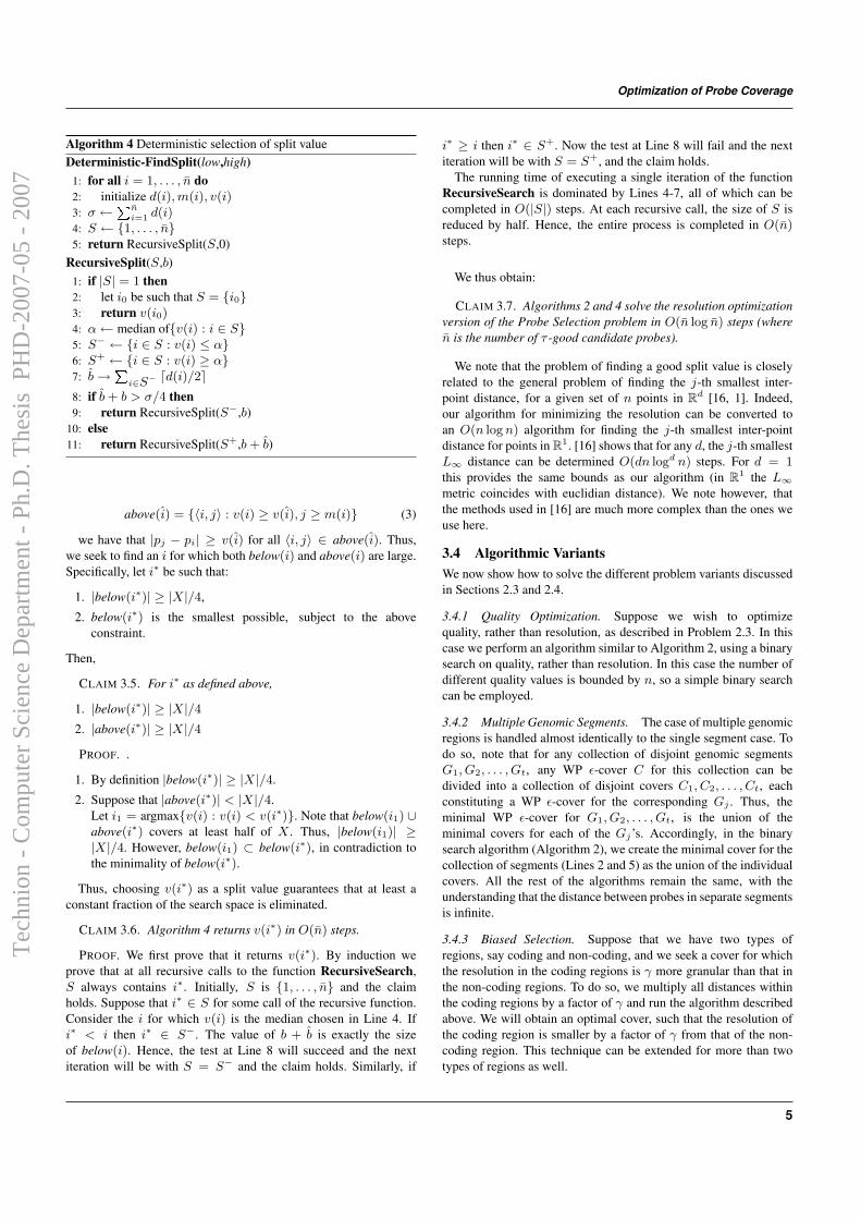
Optimization of Probe Coverage
Algorithm 4 Deterministic selection of split valueDeterministic-FindSplit(low,high)
1: for all i = 1, . . . , n do2: initialize d(i), m(i), v(i)3: σ ←
Pni=1 d(i)
4: S ← {1, . . . , n}5: return RecursiveSplit(S,0)
RecursiveSplit(S,b)1: if |S| = 1 then2: let i0 be such that S = {i0}3: return v(i0)4: α← median of{v(i) : i ∈ S}5: S− ← {i ∈ S : v(i) ≤ α}6: S+ ← {i ∈ S : v(i) ≥ α}7: b→
Pi∈S− dd(i)/2e
8: if b + b > σ/4 then9: return RecursiveSplit(S−,b)
10: else11: return RecursiveSplit(S+,b + b)
above(i) = {〈i, j〉 : v(i) ≥ v(i), j ≥ m(i)} (3)
we have that |pj − pi| ≥ v(i) for all 〈i, j〉 ∈ above(i). Thus,we seek to find an i for which both below(i) and above(i) are large.Specifically, let i∗ be such that:
1. |below(i∗)| ≥ |X|/4,
2. below(i∗) is the smallest possible, subject to the aboveconstraint.
Then,
CLAIM 3.5. For i∗ as defined above,
1. |below(i∗)| ≥ |X|/4
2. |above(i∗)| ≥ |X|/4
PROOF. .
1. By definition |below(i∗)| ≥ |X|/4.
2. Suppose that |above(i∗)| < |X|/4.Let i1 = argmax{v(i) : v(i) < v(i∗)}. Note that below(i1) ∪above(i∗) covers at least half of X . Thus, |below(i1)| ≥|X|/4. However, below(i1) ⊂ below(i∗), in contradiction tothe minimality of below(i∗).
Thus, choosing v(i∗) as a split value guarantees that at least aconstant fraction of the search space is eliminated.
CLAIM 3.6. Algorithm 4 returns v(i∗) in O(n) steps.
PROOF. We first prove that it returns v(i∗). By induction weprove that at all recursive calls to the function RecursiveSearch,S always contains i∗. Initially, S is {1, . . . , n} and the claimholds. Suppose that i∗ ∈ S for some call of the recursive function.Consider the i for which v(i) is the median chosen in Line 4. Ifi∗ < i then i∗ ∈ S−. The value of b + b is exactly the sizeof below(i). Hence, the test at Line 8 will succeed and the nextiteration will be with S = S− and the claim holds. Similarly, if
i∗ ≥ i then i∗ ∈ S+. Now the test at Line 8 will fail and the nextiteration will be with S = S+, and the claim holds.
The running time of executing a single iteration of the functionRecursiveSearch is dominated by Lines 4-7, all of which can becompleted in O(|S|) steps. At each recursive call, the size of S isreduced by half. Hence, the entire process is completed in O(n)steps.
We thus obtain:
CLAIM 3.7. Algorithms 2 and 4 solve the resolution optimizationversion of the Probe Selection problem in O(n log n) steps (wheren is the number of τ -good candidate probes).
We note that the problem of finding a good split value is closelyrelated to the general problem of finding the j-th smallest inter-point distance, for a given set of n points in Rd [16, 1]. Indeed,our algorithm for minimizing the resolution can be converted toan O(n log n) algorithm for finding the j-th smallest inter-pointdistance for points in R1. [16] shows that for any d, the j-th smallestL∞ distance can be determined O(dn logd n) steps. For d = 1this provides the same bounds as our algorithm (in R1 the L∞metric coincides with euclidian distance). We note however, thatthe methods used in [16] are much more complex than the ones weuse here.
3.4 Algorithmic VariantsWe now show how to solve the different problem variants discussedin Sections 2.3 and 2.4.
3.4.1 Quality Optimization. Suppose we wish to optimizequality, rather than resolution, as described in Problem 2.3. In thiscase we perform an algorithm similar to Algorithm 2, using a binarysearch on quality, rather than resolution. In this case the number ofdifferent quality values is bounded by n, so a simple binary searchcan be employed.
3.4.2 Multiple Genomic Segments. The case of multiple genomicregions is handled almost identically to the single segment case. Todo so, note that for any collection of disjoint genomic segmentsG1, G2, . . . , Gt, any WP ε-cover C for this collection can bedivided into a collection of disjoint covers C1, C2, . . . , Ct, eachconstituting a WP ε-cover for the corresponding Gj . Thus, theminimal WP ε-cover for G1, G2, . . . , Gt, is the union of theminimal covers for each of the Gj’s. Accordingly, in the binarysearch algorithm (Algorithm 2), we create the minimal cover for thecollection of segments (Lines 2 and 5) as the union of the individualcovers. All the rest of the algorithms remain the same, with theunderstanding that the distance between probes in separate segmentsis infinite.
3.4.3 Biased Selection. Suppose that we have two types ofregions, say coding and non-coding, and we seek a cover for whichthe resolution in the coding regions is γ more granular than that inthe non-coding regions. To do so, we multiply all distances withinthe coding regions by a factor of γ and run the algorithm describedabove. We will obtain an optimal cover, such that the resolution ofthe coding region is smaller by a factor of γ from that of the non-coding region. This technique can be extended for more than twotypes of regions as well.
5
Tec
hnio
n -
Com
pute
r Sc
ienc
e D
epar
tmen
t - P
h.D
. The
sis
PH
D-2
007-
05 -
200
7
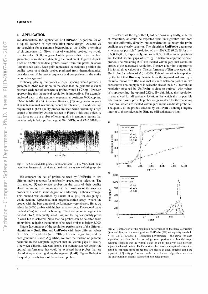
Lipson et al
4 APPLICATIONWe demonstrate the application of UniProbe (Algorithm 2) ona typical scenario of high-resolution probe design. Assume weare searching for a genomic breakpoint at the 6Mbp p-terminusof chromosome 10. Given a set of candidate probes, we wouldlike to select 3,000 oligonucleotide probes that offer the bestguaranteed resolution of detecting the breakpoint. Figure 1 depictsa set of 82,500 candidate probes, taken from our probe database(unpublished data). Each point represents the genomic position andquality score of a single probe, predicted from thermodynamicalconsideration of the probe sequence and comparison to the entiregenome background.
In theory, placing the probes at equal spacing would provide aguaranteed 2Kbp resolution, in the sense that the genomic distancebetween each pair of consecutive probes would be 2Kbp. However,approaching this theoretical resolution is impossible. For example,unclosed gaps in the genomic sequence at positions 0–50Kbp and5.63–5.68Mbp (UCSC Genome Browser, [7]) are genomic regionsat which maximal resolution cannot be obtained. In addition, werequire that highest quality probes are used while sustaining a highdegree of uniformity. As can be seen in Figure 1 this dual objectivemay force us to use probes of lower quality in genomic regions thatcontain only inferior probes, e.g. at 50–130Kbp or 4.97–5.07Mbp.
Fig. 1. 82,500 candidate probes in chromosome 10 0-6 Mbp. Each pointrepresents the genomic position and predicted quality score of a single probe.
We compare the set of probes selected by UniProbe to twodifferent naive methods for uniformly-spaced probe selection. Thefirst method (Qual) selects probes on the basis of their qualityalone, assuming that randomness in the positions of the superiorprobes will lead to some degree of uniformity in their coverage.This method was described by Lucito et al [10] for designing awhole-genome representational oligonucleotide array, where theprobes with the best empirical performance were chosen. Here, weselect the 3,000 probes with highest quality score. The second naivemethod (Bin) is based on binning: The total genomic segment isdivided into 3,000 equally-sized bins, and the highest-quality probein each bin is selected. Note that no probes can be selected fromempty bins, reducing the number of selected probes to below 3,000.
Figure 2a compares of the resolution performance of the differentalgorithms – Qual, Bin, and UniProbe with three different valuesof τ : 0.5, 0.75 and 0.85 (w = 2Kbp). For each algorithm, and foreach genomic distance d ≤ 6Kbp, we note the fraction of genomicpositions in the complete segment that lie within gaps of size ≤d between adjacent selected probe. For comparison we depict theoptimal performance that could be expected from probes that areplaced at equal spacing along the segment (Unif). Figure 2b depictsthe quality distributions of the selected probes.
It is clear that the algorithm Qual performs very badly, in termsof resolution, as could be expected from an algorithm that doesnot take uniformity directly into consideration, although the probequalities are clearly superior. The algorithm UniProbe guaranteesa “whenever possible” resolution of ε = 2085, 2186, 2258 for τ =0.5, 0.75, 0.85, respectively, and some 80% of all genomic positionsare located within gaps of size ≤ ε between adjacent selectedprobes. The remaining 20% are located within gaps that cannot beprobed at the guaranteed resolution. The new algorithm outperformsBin for all three values of τ . The performance of Bin converges withUniProbe for values of d > 4000. This observation is explainedby the fact that Bin may deviate from the optimal solution by amaximal factor of 2 (the maximal distance between probes in twoconsecutive non-empty bins is twice the size of the bin). Overall, theresolution obtained by UniProbe is close to optimal, with valuesof ε approaching the optimal 2Kbp. By definition, this resolutionis guaranteed for all genomic locations for which this is possiblewhereas the closest possible probes are guaranteed for the remaininglocations, which are located within gaps in the candidate probe set.The quality of the probes selected by UniProbe , although slightlyinferior to those selected by Bin, are still satisfactory high.
Fig. 2. Comparison of the resolution performance of the naive algorithmsQual and Bin, and the new algorithm UniProbe (UP) with quality thresholdτ = 0.5, 0.75, 0.85. a) Resolution performance – the curve for eachalgorithm describes the fraction of genomic positions within the targetgenomic segment that lie within a gap of up to the given size betweenadjacent selected probes. Unif describes the theoretical optimal result thatcould be expected from probes that are placed at equal spacing along thesegment. b) Quality performance – the curve for each algorithm describesthe distribution of quality scores of the selected probes.
6
Tec
hnio
n -
Com
pute
r Sc
ienc
e D
epar
tmen
t - P
h.D
. The
sis
PH
D-2
007-
05 -
200
7
Optimization of Probe Coverage
REFERENCES[1]P.K. Agarwal, B. Aronov, M. Sharir, and S. Suri. Selecting distances in the plane.
Algorithmica, 9(5):495–514, 1993.[2]B.R. Balsara and J.R. Testa. Chromosomal imbalances in human lung cancer.
Oncogene, 21(45):6877–83, 2002.[3]M.T. Barrett, A. Scheffer, A. Ben-Dor, N. Sampas, D. Lipson, R. Kincaid,
P. Tsang, B. Curry, K. Baird, P.S. Meltzer, Z. Yakhini, L. Bruhn, and S. Laderman.Comparative genomic hybridization using oligonucleotide microarrays and totalgenomic DNA. PNAS, 101(51):17765–17770, 2004.
[4]G.R. Bignell, J. Huang, J. Greshock, S. Watt, A. Butler, S. West, M. Grigorova,K.W. Jones, W. Wei, M.R. Stratton, P.A. Futreal, B. Weber, M.H. Shapero, andR. Wooster. High-resolution analysis of DNA copy number using oligonucleotidemicroarrays. Genome Res, 14(2):287–95, 2004.
[5]C. Brennan, Y. Zhang, C. Leo, B. Feng, C. Cauwels, A.J. Aguirre, M. Kim,A. Protopopov, and L. Chin. High-resolution global profiling of genomicalterations with long oligonucleotide microarray. Cancer Res, 64(14):4744–8,2004.
[6]O.P. Kallioniemi, A. Kallioniemi, D. Sudar, D. Rutovitz, J.W. Gray, F. Waldman,and D. Pinkel. Comparative genomic hybridization: a rapid new method fordetecting and mapping DNA amplification in tumors. Semin Cancer Biol,4(1):41–46, 1993.
[7]W.J. Kent, C.W. Sugnet, T.S. Furey, K.M. Roskin, T.H. Pringle, A.M. Zahler, andD. Haussler. The human genome browser at UCSC. Genome Res, 12(6):996–1006, 2002.
[8]F. Li and G.D. Stormo. Selection of optimal DNA oligos for gene expressionarrays. Bioinformatics, 17(1):1067–1076, 2001.
[9]D. Lipson, P. Webb, and Z. Yakhini. Designing specific oligonucleotide probesfor the entire S. cerevisiae transcriptome. In Second Workshop on Algorithms in
Bioinformatics (WABI 02), LNCS 2452, pages 491–505. Springer-Verlag, 2002.[10]R. Lucito, J. Healy, J. Alexander, A. Reiner, D. Esposito, M. Chi, L. Rodgers,
A. Brady, J. Sebat, J. Troge, J.A. West, S. Rostan, K.C.Q. Nguyen, S. Powers,K.Q. Ye, A. Olshen, E. Venkatraman, L. Norton, and M. Wigler. Representationaloligonucleotide microarray analysis: A high-resolution method to detect genomecopy number variation. Genome Res., 13:2291–2305, 2003.
[11]R. Mei, E. Hubbell, S. Bekiranov, M. Mittmann, F.C. Christians, M. Shen, G. Lu,J. Fang, W. Liu, T. Ryder, P. Kaplan, D. Kulp, and T.A. Webster. Probe selectionfor high-density oligonucleotide arrays. PNAS, 100(20):11237–11242, 2003.
[12]F. Mertens, B. Johansson, M. Hoglund, and F. Mitelman. Chromosomal imbalancemaps of malignant solid tumors: a cytogenetic survey of 3185 neoplasms. CancerRes, 57(13):2765–80, 1997.
[13]D. Pinkel, R. Segraves, D. Sudar, S. Clark, I. Poole, D. Kowbel, C. Collins,W.L. Kuo, C. Chen, Y. Zhai, S.H. Dairkee, B.M. Ljung, J.W. Gray, andD.G. Albertson. High resolution analysis of DNA copy number variation usingcomparative genomic hybridization to microarrays. Nat Genet, 20(2):207–211,1998.
[14]J.R. Pollack, C.M. Perou, A.A. Alizadeh, M.B. Eisen, A. Pergamenschikov, C.F.Williams, S.S. Jeffrey, D. Botstein, and P.O. Brown. Genome-wide analysis ofDNA copy-number changes using cDNA microarrays. Nat Genet, 23(1):41–6,1999.
[15]J. Rouillard, M. Zuker, and E. Gulari. Oligoarray 2.0: design of oligonucleotideprobes for DNA microarrays using a thermodynamic approach. Nucleic Acids Res,31(12):3057–3062, 2003.
[16]J.S. Salowe. L-infinity interdistance selection by parametric search. InformProcess Lett, 30(1):9–14, 1989.
7
Tec
hnio
n -
Com
pute
r Sc
ienc
e D
epar
tmen
t - P
h.D
. The
sis
PH
D-2
007-
05 -
200
7

Tec
hnio
n -
Com
pute
r Sc
ienc
e D
epar
tmen
t - P
h.D
. The
sis
PH
D-2
007-
05 -
200
7
A.3 Efficient Calculation of Interval Scores
for DNA Copy Number Data Analysis
Doron Lipson, Yonatan Aumann, Amir Ben-Dor, Nathan Linial, and ZoharYakhini. “Efficient Calculation of Interval Scores for DNA CopyNumber Data Analysis”. Proceedings of RECOMB ’05, LNCS 3500, p.83, Springer-Verlag, 2005. Also in Journal of Computational Biology, Vol.13, No. 2: 215-228, 2006.
89
Tec
hnio
n -
Com
pute
r Sc
ienc
e D
epar
tmen
t - P
h.D
. The
sis
PH
D-2
007-
05 -
200
7

90
Tec
hnio
n -
Com
pute
r Sc
ienc
e D
epar
tmen
t - P
h.D
. The
sis
PH
D-2
007-
05 -
200
7

Efficient Calculation of Interval Scores for DNA Copy Number DataAnalysis
Doron Lipson∗ Yonatan Aumann† Amir Ben-Dor‡ Nathan Linial§ Zohar Yakhini¶
Keywords: CGH, genome rearrangements, cancer, microarray analysis, optimization, approximation
Abstract
Background. DNA amplifications and deletions characterize cancer genome and are often related to disease evolu-tion. Microarray based techniques for measuring these DNA copy-number changes use fluorescence ratios at arrayedDNA elements (BACs, cDNA or oligonucleotides) to provide signals at high resolution, in terms of genomic locations.These data are then further analyzed to map aberrations and boundaries and identify biologically significant structures.
Methods. We develop a statistical framework that enables the casting of several DNA copy number data analysisquestions as optimization problems over real valued vectors of signals. The simplest form of the optimization problemseeks to maximizeϕ(I) =
∑vi/√|I| over all subintervalsI in the input vector. We present and prove a linear time
approximation scheme for this problem. Namely, a process with time complexityO(nε−2
)that outputs an interval for
whichϕ(I) is at least Opt/α(ε), where Opt is the actual optimum andα(ε)→ 1 asε→ 0. We further develop practicalimplementations that improve the performance of the naive quadratic approach by orders of magnitude. We discussproperties of optimal intervals and how they apply to the algorithm performance.
Examples. We benchmark our algorithms on synthetic as well as publicly available DNA copy number data. Wedemonstrate the use of these methods for identifying aberrations in single samples as well as common alterations infixed sets and subsets of breast cancer samples.
∗Computer Science Dept., Technion, Haifa ([email protected] ), corresponding author.†Computer Science Dept., Bar-Ilan University, Ramat Gan ([email protected] ).‡Agilent Laboratories (amir [email protected] ).§Computer Science Dept., Hebrew University of Jerusalem ([email protected] ).¶Agilent Laboratories and Computer Science Dept., Technion, Haifa (zohar [email protected] )
1
Tec
hnio
n -
Com
pute
r Sc
ienc
e D
epar
tmen
t - P
h.D
. The
sis
PH
D-2
007-
05 -
200
7
1 Introduction
Alterations in DNA copy number are characteristic of many cancer types and are thought to drive some cancer patho-genesis processes. These alterations include large chromosomal gains and losses as well as smaller scale amplificationsand deletions. Because of their role in cancer development, regions of chromosomal instability are useful for elucidatingother components of the process. For example, since genomic instability can trigger the over expression or activationof oncogenes and the silencing of tumor suppressors, mapping regions of common genomic aberrations has been usedto discover cancer related genes. Understanding genome aberrations is important for both the basic understanding ofcancer and for diagnosis and clinical practice.
Alterations in DNA copy number have been initially measured using local fluorescence in situ hybridization-basedtechniques. These evolved to a genome wide technique called Comparative Genomic Hybridization (CGH, see [11]),now commonly used for the identification of chromosomal alterations in cancer [14, 1]. In this genome-wide cytogeneticmethod differentially labeled tumor and normal DNA are co-hybridized to normal metaphases. Ratios between the twolabels allow the detection of chromosomal amplifications and deletions of regions that may harbor oncogenes andtumor suppressor genes. Classical CGH has, however, a limited resolution (10-20 Mbp). With such low resolutionit is impossible to predict the borders of the chromosomal changes or to identify changes in copy numbers of singlegenes and small genomic regions. In a more advanced method termed array CGH (aCGH), tumor and normal DNA areco-hybridized to a microarray of thousands of genomic clones of BAC, cDNA or oligonucleotide probes [18, 9, 16, 7,10, 2, 6]. The use of aCGH allows the determination of changes in DNA copy number of relatively small chromosomalregions. Using oligonucleotides arrays the resolution can, in theory, be finer than single genes.
To fully realize the advantages associated with the emerging high resolution technologies, practitioners need ap-propriate efficient data analysis methods. A common first step in analyzing DNA copy number (DCN) data consistsof identifying aberrant (amplified or deleted) regions in each individual sample. Indeed, current literature on analyz-ing DCN data describes several approaches to this task, based on a variety of optimization techniques. Hupe et al[15] develop a methodology for automatic detection of breakpoints and aberrant regions, based on Adaptive WeightSmoothing ([20]), a segmentation technique that fits a piecewise constant function to an input function. The fit is basedon maximizing the likelihood of the (observed) function given the piecewise constant model, penalized for the numberof transitions. The penalty weight is a parameter of the process. Sebat et al [10], in a pioneering paper, study DCNvariations that naturally occur in normal populations. Using an HMM based approach they compare signals for twoindividuals and seek intervals of 4 or more probes in which DCNs are likely to be different. A common shortcomingof many other current approaches is lack of principled optimization criteria that drive the method. Even when a figureof merit forms the mathematical basis of the process such as in [10], convergence of the optimization process is notguaranteed.
Further steps in analyzing DCN data include the automatic elucidation of more complex structures. A central taskinvolves the discovery of common aberrations, either in a fixed set of studied samples or in an unsupervised mode,where we search for intervals that are aberrant in some significant subset of the samples. There are no formal treatmentsof this problem in the literature but most studies do report common aberrations and their locations. The relationship ofDCN variation and expression levels of genes that reside in the aberrant region is of considerable interest. By measuringDNA copy numbers and mRNA expression levels on the same set of samples we gain access to the relationship of copynumber alterations to how they are manifested in altering expression profiles. In [17] the authors used (metaphase slides)CGH to identify large scale amplifications in 23 metastatic colon cancer samples. For each identified large amplifiedregion they compared the median expression levels of genes that reside there (2146 genes total), in the samples whereamplification was detected, to the median expression levels of these genes in 9 normal control colon samples. A 2-foldover-expression was found in 81 of these genes. No quantitative statistical assessment of the results is given. In [19]a more decisive observation is reported. For breast cancer samples the authors establish a strong global correlationbetween copy number changes and expression level variation. Hyman et al [9] report similar findings. The statisticsused by both latter studies is based on simulations and takes into account single gene correlations but not local regionaleffects. In Section 2.3 we show how our general framework enables us to efficiently compute correlations between geneexpression vectors and DCN vectors of genomic intervals, greatly extending the scope of the analysis.
2
Tec
hnio
n -
Com
pute
r Sc
ienc
e D
epar
tmen
t - P
h.D
. The
sis
PH
D-2
007-
05 -
200
7
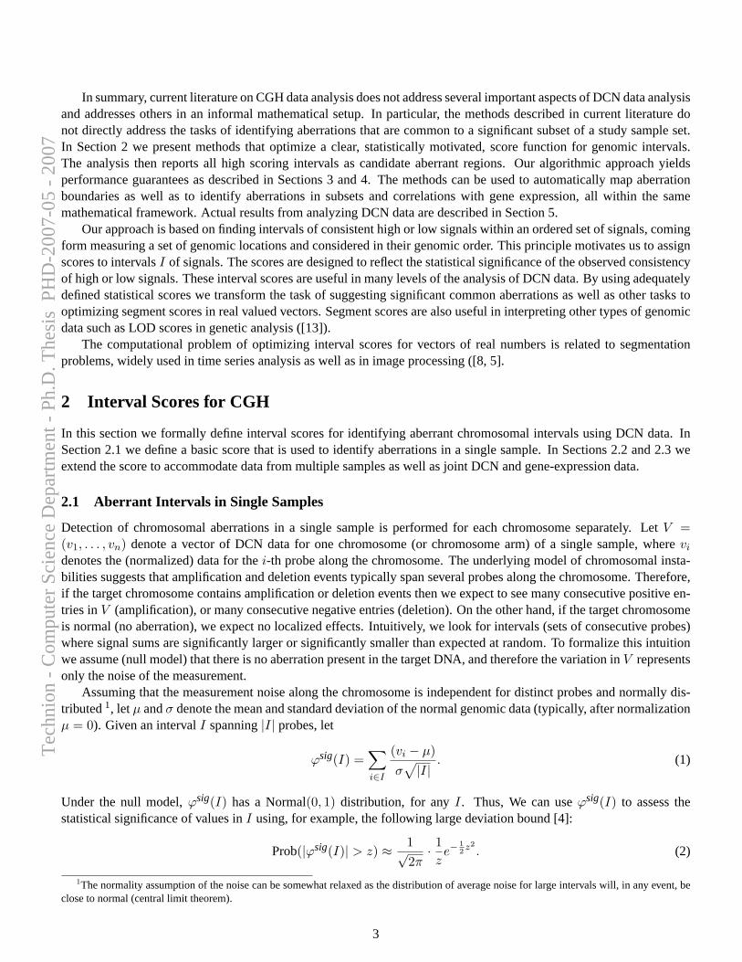
In summary, current literature on CGH data analysis does not address several important aspects of DCN data analysisand addresses others in an informal mathematical setup. In particular, the methods described in current literature donot directly address the tasks of identifying aberrations that are common to a significant subset of a study sample set.In Section 2 we present methods that optimize a clear, statistically motivated, score function for genomic intervals.The analysis then reports all high scoring intervals as candidate aberrant regions. Our algorithmic approach yieldsperformance guarantees as described in Sections 3 and 4. The methods can be used to automatically map aberrationboundaries as well as to identify aberrations in subsets and correlations with gene expression, all within the samemathematical framework. Actual results from analyzing DCN data are described in Section 5.
Our approach is based on finding intervals of consistent high or low signals within an ordered set of signals, comingform measuring a set of genomic locations and considered in their genomic order. This principle motivates us to assignscores to intervalsI of signals. The scores are designed to reflect the statistical significance of the observed consistencyof high or low signals. These interval scores are useful in many levels of the analysis of DCN data. By using adequatelydefined statistical scores we transform the task of suggesting significant common aberrations as well as other tasks tooptimizing segment scores in real valued vectors. Segment scores are also useful in interpreting other types of genomicdata such as LOD scores in genetic analysis ([13]).
The computational problem of optimizing interval scores for vectors of real numbers is related to segmentationproblems, widely used in time series analysis as well as in image processing ([8, 5].
2 Interval Scores for CGH
In this section we formally define interval scores for identifying aberrant chromosomal intervals using DCN data. InSection 2.1 we define a basic score that is used to identify aberrations in a single sample. In Sections 2.2 and 2.3 weextend the score to accommodate data from multiple samples as well as joint DCN and gene-expression data.
2.1 Aberrant Intervals in Single Samples
Detection of chromosomal aberrations in a single sample is performed for each chromosome separately. LetV =(v1, . . . , vn) denote a vector of DCN data for one chromosome (or chromosome arm) of a single sample, wherevi
denotes the (normalized) data for thei-th probe along the chromosome. The underlying model of chromosomal insta-bilities suggests that amplification and deletion events typically span several probes along the chromosome. Therefore,if the target chromosome contains amplification or deletion events then we expect to see many consecutive positive en-tries inV (amplification), or many consecutive negative entries (deletion). On the other hand, if the target chromosomeis normal (no aberration), we expect no localized effects. Intuitively, we look for intervals (sets of consecutive probes)where signal sums are significantly larger or significantly smaller than expected at random. To formalize this intuitionwe assume (null model) that there is no aberration present in the target DNA, and therefore the variation inV representsonly the noise of the measurement.
Assuming that the measurement noise along the chromosome is independent for distinct probes and normally dis-tributed1, letµ andσ denote the mean and standard deviation of the normal genomic data (typically, after normalizationµ = 0). Given an intervalI spanning|I| probes, let
ϕsig(I) =∑i∈I
(vi − µ)σ√|I|
. (1)
Under the null model,ϕsig(I) has a Normal(0, 1) distribution, for anyI. Thus, We can useϕsig(I) to assess thestatistical significance of values inI using, for example, the following large deviation bound [4]:
Prob(|ϕsig(I)| > z) ≈ 1√2π· 1ze−
12z2
. (2)
1The normality assumption of the noise can be somewhat relaxed as the distribution of average noise for large intervals will, in any event, beclose to normal (central limit theorem).
3
Tec
hnio
n -
Com
pute
r Sc
ienc
e D
epar
tmen
t - P
h.D
. The
sis
PH
D-2
007-
05 -
200
7

Given a vector of measured DCN dataV , we therefore seek all intervalsI with ϕsig(I) exceeding a certain threshold.Setting the threshold to avoid false positives we report all these intervals as putative aberrations.
2.2 Aberrant Intervals in Multiple Samples
When DCN data from multiple samples is available it may, of course, be processed one sample at a time. However, itis possible to take advantage of the additional data to increase the significance of the located aberrations by searchingfor commonaberrations. More important than the statistical advantage, common aberrations are indicative of genomicalterations selected for in the tumor development process and may therefore be of higher biological relevance.
Given a set of samplesS, and a matrixV = {vs,i} of CGH values wherevs,i denotes the (normalized) data for thei-th probe in samples ∈ S, identification of common aberrations may be done in one of two modes. In thefixed setmode we search for genomic intervals that are significantly aberrant (either amplified or deleted) in all samples inS. Intheclass discoverymode we search for genomic intervalsI for which there exists a subset of the samplesC ⊆ S suchthatI is significantly aberrant only in the samples withinC.
2.2.1 Fixed Set of Samples
A simple variant of the single-sample score (1) allows accommodation of multiple samples. Given an intervalI, let
ϕsigS (I) =
∑s∈S
∑i∈I
(vs,i − µ)σ√|I| · |S|
. (3)
Although this score will indeed indicate whetherI contains a significant aberration within the samples inS, it does nothave the ability to discern between anuncommonaberration that is highly manifested in only one sample, and acommonaberration that has a more moderate effect on all samples. In order to focus on common aberrations, we employ arobustvariant of the score: Given some thresholdτ+, we create a binary dataset:B = {bs,i} wherebs,i = 1 if vs,i > τ+
andbs,i = 0 otherwise. Assuming (null model) that the appearance of 1s inB is independent for distinct probes andsamples we expect the number of positive values in the submatrix defined byI × S to be Binom(n, p) distributed withn = |I| · |S| andp = Prob(vs,i > τ+) =
∑s∈S
∑ni=1
bs,i
|B| . The significance ofk 1s inI × S can be assessed by thebinomial tail probability:
n∑i=k
(n
i
)pi(1− p)(n−i). (4)
For algorithmic convenience we utilize the Normal approximation of the above [3]. Namely, for each probei we definethe score of an intervalI as in (3):
ϕrobS (I) =
∑s∈S
∑i∈I
(bs,i − ν)ρ√|I| · |S|
, (5)
whereν = p andρ =√
p(1− p) are the mean and standard deviation of the variablesbs,i. A high scoreϕrobS (I) is
indicative of a common amplification inI. A similar score indicates deletions using a negative thresholdτ−.
2.2.2 Class Discovery
In the mode of class discovery we search a genomic intervalI and a subsetC ⊆ S such thatI is significantly aberranton the samples withinC. Formally, we search for a pair(I, C) that maximizes the score:
ϕsig(I, C) =∑s∈C
∑i∈I
(vs,i − µ)σ√|I| · |C|
. (6)
A robustform of this score is:
ϕrob(I, C) =∑s∈C
∑i∈I
(bs,i − ν)ρ√|I| · |C|
. (7)
4
Tec
hnio
n -
Com
pute
r Sc
ienc
e D
epar
tmen
t - P
h.D
. The
sis
PH
D-2
007-
05 -
200
7

2.3 Regional Correlation to Gene Expression
In previous work [12] we introduced the Regional Correlation Score as a measure of correlation between the expressionlevels pattern of a gene and an aberration in or close to its genomic locus. For any given geneg, with a known genomiclocation, the goal is to find whether there is an aberration in its chromosome that potentially effects the transcriptionlevels ofg. Formally, we are given a vectore of expression level measurements ofg over a set samplesS, and a setof vectorsV = (v1, ..., vn) of the same length corresponding to genomically ordered probes on the same chromosome,where each vector contains DCN values over the same set of samplesS. For a genomic intervalI ⊂ [1, ..., n] we definea regional correlation score:
ϕcor(I, e) =∑
i∈I r(e, vi)√|I|
, (8)
wherer(e, vi) is some correlation score (e.g. Pearson correlation) between the vectorse andvi. We are interestedin determining whether there is some intervalI for which ϕcor(I, e) is significantly high. Note that for this decisionproblem it is sufficient to use an approximation process, such as described in Section 3.
2.4 A Tight Upper Bound for the Number of Optimal Intervals
In general, we are interested in finding the interval with the maximal score. A natural question is thus what is the maxi-mal possible number of intervals with maximal score. The following theorem, proof of which appears in Appendix A,provides a tight bound on this number.
Theorem 2.1. Given any of the above scores, there can ben and at mostn maximal intervals.
3 Approximation Scheme
In the previous section we described interval scores arising from several different motivations related to the analysisDCN data. Despite the varying settings, the form of the interval scores in the different cases is similar. We are interestedin finding the interval with maximal score. Clearly, this can be done by exhaustive search, checking all possible intervals.However, even for the single sample case this would takeΘ(n2) steps, which rapidly becomes time consuming, as thenumber of measured genomic loci grows to tens of thousands. Moreover, even forn ≈ 104, Θ(n2) does not allowfor interactive data analysis, which is called for by practitioners. For the class discovery case, a naive solution wouldrequire an exponentialΘ(n22|S|) number of steps. Thus, we seek more efficient algorithms. In this section we presenta linear time approximation scheme. Then, based on this approximation scheme, we show how to efficiently find theactual optimal interval.
3.1 Fixed Sample Set
Note that the single sample case is a specific case of the fixed multiple-sample case (|S| = 1), on which we concentrate.For this case there are two interval scores defined in Section 2.2. The optimization problem for both these scores,as well as the score for regional correlations of Section 2.3, can all be cast as a general optimization problem. LetW = (w1, . . . , wn) be a sequence of numbers. For an intervalI define
ϕ(I) =∑
i∈I wi√|I|
(9)
Settingwi =∑
s∈S(vs,i−µ)
σ√|S|
gives ϕ(I) = ϕsigS (I); settingwi =
∑s∈S(bs,i−ν)
ρ√|S|
gives ϕ(I) = ϕrobS (I); and setting
wi = r(e, vi) givesϕ(I) = ϕcor(I, e). Thus, we focus on the problem of optimizingϕ(I) for a general sequenceW .
5
Tec
hnio
n -
Com
pute
r Sc
ienc
e D
epar
tmen
t - P
h.D
. The
sis
PH
D-2
007-
05 -
200
7

3.1.1 A Geometric Family of Intervals
For an intervalI = [x, y] definesum(I) =∑y
i=x wi. Fix ε > 0. We define a familyI of intervals of increasing lengths,thegeometric family, as follows. For integralj, let kj = (1 + ε)j and∆j = εkj . Forj = 0, . . . , log(1+ε) n, let
I(j) ={
[i∆j , i∆j + kj − 1] : 0 ≤ i ≤ n− kj
∆j
}In words,I(j) consists of intervals of sizekj evenly spaced∆j apart. SetI = ∪log(1+ε) n
j=0 I(j). The following lemmashows that any intervalI ⊆ [1..n] contains an interval ofI that has “almost” the same size.
Lemma 3.1. LetI be an interval, andJ – the leftmost longest interval ofI fully contained inI. Then|I|−|J ||I| ≤ 2ε+ ε2.
Proof. Let j be such that|J | = kj . In I there is an interval of sizekj+1 every∆j+1 steps. Thus, since there are nointervals of sizekj+1 contained inI, it must be that|I| < kj+1 + ∆j+1. Therefore
|I| − |J | < kj+1 + ∆j+1 − kj = (1 + ε)kj + ε(1 + ε)kj − kj = (2ε + ε2)kj ≤ (2ε + ε2)|I| �
3.1.2 The Approximation Algorithm for a Fixed Set
The approximation algorithm simply computes scores for allJ ∈ I and outputs the highest scoring one:
Algorithm 1 Approximation Algorithm - Fixed Sample CaseInput: SequenceW = {wi}.Output: IntervalJ with score approximating the optimal score.
sum([1, 0]) = 0for j = 1 to n sum([1, j]) = sum([1, j − 1]) + wj
ForeachJ = [x, y] ∈ I ϕ(J) =sum([1, y])−sum([1, x− 1])
|I|1/2
output Jmax = argmaxJ∈I{ϕ(J)}
The approximation guarantee of the algorithm is based on the following lemma:
Lemma 3.2. For ε ≤ 1/5 the following holds. LetI∗ be an interval with the optimal score and letJ be the leftmostlongest interval ofI contained inI. Thenϕ(J) ≥ ϕ(I∗)/α, with α = (1−
√2ε(2 + ε))−1.
Proof. SetM∗ = ϕ(I∗). Assume by contradiction thatϕ(J) < M∗/α. DenoteJ = [u, v] andI∗ = [x, y]. DefineA = [x, u− 1] andB = [v + 1, y] (the segments ofI∗ protruding beyondJ to the left and right). We have,
M∗ = ϕ(I∗) =sum(A) + sum(J) + sum(B)
|I∗|1/2=
sum(A)|A|1/2
· |A|1/2
|I∗|1/2+
sum(J)|J |1/2
· |J |1/2
|I∗|1/2+
sum(B)|B|1/2
· |B|1/2
|I∗|1/2
≤ ϕ(A) · |A|1/2
|I∗|1/2+ ϕ(J) · |J |
1/2
|I∗|1/2+ ϕ(B) · |B|
1/2
|I∗|1/2
≤ M∗ |A|1/2
|I∗|1/2+ ϕ(J)
|J |1/2
|I∗|1/2+ M∗ |B|1/2
|I∗|1/2≤
(|A|1/2 + |B|1/2
|I∗|1/2
)M∗ + ϕ(J) (10)
≤(|A|+ |B||I∗|
)1/2√2M∗ + ϕ(J) (11)
≤√
2(2ε + ε2) ·M∗ + ϕ(J), (12)
<√
2(2ε + ε2) ·M∗ + M∗/α = M∗, (13)
in contradiction. In the above, (10) follows from the optimality ofM∗; (11) follows from arithmetic-geometric meansinequality; (12) follows from Lemma 3.1; and (13) by the contradiction assumption and by the definition ofα. �
Thus, since the optimal interval must contain at least one interval ofI, we get,
6
Tec
hnio
n -
Com
pute
r Sc
ienc
e D
epar
tmen
t - P
h.D
. The
sis
PH
D-2
007-
05 -
200
7

Theorem 3.3. For ε ≤ 1/5, Algorithm 1 provides anα(ε) = (1−√
2ε(2 + ε))−1 approximation to the maximal score.
Note thatα(ε)→ 1 asε→ 0. Hence, the above constitutes an approximation scheme.
Complexity. The complexity of the algorithm is determined by the number of intervals inI. For eachj, the intervalsof Ij are∆j apart. Thus,|Ij | ≤ n
∆j= n
ε(1+ε)j . Hence, the total complexity of the algorithm is:
|I| ≤log(1+ε) n∑
j=0
n
ε(1 + ε)−j ≤ n
ε
∞∑j=0
(1 + ε)−j = ε−2n = O(nε−2)
3.2 Class Discovery
Consider the problem of optimizing the scoresϕsig(I, C) and ϕrob(I, C). Similar to the fixed sample case, bothproblems can be cast as an instance of the general optimization problem. For an intervalI andC ⊆ S let:
ϕ(I, C) =
∑i∈I,s∈C ws,i√|I| · |C|
, opt(I) = maxC⊆S
ϕ(I, C)
Note thatmaxI,C{ϕ(I, C)} = maxI{opt(I)}.
3.2.1 Computingopt(I)
We now show how to efficiently computeopt(I), without actually checking all possible subsetsC ⊆ S. The key ideais the following. Note that for anyC, ϕ(I, C) =
∑s∈C sums(I)/(|C||I|)1/2. Thus, for a fixed|C| = k, ϕ(I, C) is
maximized by takingk s’s with the largestsums(I). Thus, we need only sort the samples by this order, and considerthe|S| possible sizes, which is done inO(|S| log |S|). A description of the algorithm is provided in Appendix B.
3.2.2 The Approximation Algorithm for Class Discovery
Recall the geometric family of intervalsI, as defined in Section 3.1. For the approximation algorithm, for eachJ ∈ Icomputeopt(J). Let Jmax be the interval with the largestopt(J). Using the Algorithm 4 find theC for which opt(J)is obtained, and output the pairJ,C. The approximation ratio obtained for the class discovery case is identical to thatof the fixed case, and the analysis is also very similar.
Theorem 3.4. For any ε ≤ 1/5, the above algorithm provides anα(ε) = (1 −√
2ε(2 + ε))−1 approximation to themaximal score.
The proof, which is essentially identical to that of Theorem 3.3, is omitted. Again, sinceα(ε) approaches 1 asεapproaches 0, the above constitutes an approximation scheme.
Complexity. Computingϕ([1, j], s) for j = 1, . . . , n, takesO(|S|n) steps. For eachJ ∈ I computingopt(J) isO(|S| log |S|). There areO(nε−2) intervals inI. Thus, the total number of steps for the algorithm isO(n|S| log |S|ε−2).
4 Finding the Optimal Interval
In the previous section we showed how toapproximatethe optimal score. We now show how to find the absolute optimalscore and interval. We present two algorithms. First, we present theLookAheadalgorithm. Then, we present the GFA(Geometric Family Algorithm) which is based on a combination of theLookAheadalgorithm, and the approximationalgorithm described above. We note that for both algorithms we cannot prove that their worst case performance is betterthanO(n2), but in Section 5 we show that in practiceLookAheadrun inO(n1.5) and GFA runs in linear time.
7
Tec
hnio
n -
Com
pute
r Sc
ienc
e D
epar
tmen
t - P
h.D
. The
sis
PH
D-2
007-
05 -
200
7
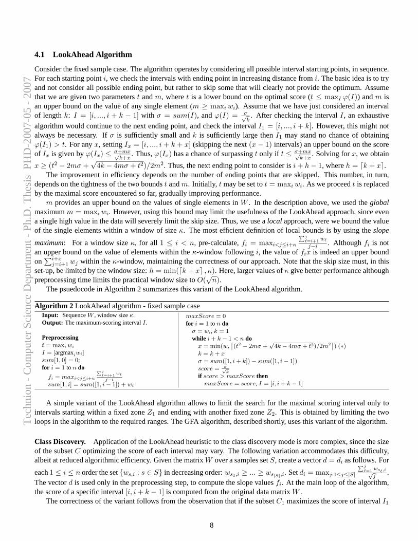
4.1 LookAhead Algorithm
Consider the fixed sample case. The algorithm operates by considering all possible interval starting points, in sequence.For each starting pointi, we check the intervals with ending point in increasing distance fromi. The basic idea is to tryand not consider all possible ending point, but rather to skip some that will clearly not provide the optimum. Assumethat we are given two parameterst andm, wheret is a lower bound on the optimal score (t ≤ maxI ϕ(I)) andm isan upper bound on the value of any single element (m ≥ maxi wi). Assume that we have just considered an intervalof lengthk: I = [i, ..., i + k − 1] with σ = sum(I), andϕ(I) = σ√
k. After checking the intervalI, an exhaustive
algorithm would continue to the next ending point, and check the intervalI1 = [i, ..., i + k]. However, this might notalways be necessary. Ifσ is sufficiently small andk is sufficiently large thenI1 may stand no chance of obtainingϕ(I1) > t. For anyx, settingIx = [i, ..., i + k + x] (skipping the next(x − 1) intervals) an upper bound on the scoreof Ix is given byϕ(Ix) ≤ σ+mx√
k+x. Thus,ϕ(Ix) has a chance of surpassingt only if t ≤ σ+mx√
k+x. Solving forx, we obtain
x ≥ (t2 − 2mσ +√
4k − 4mσ + t2)/2m2. Thus, the next ending point to consider isi + h− 1, whereh = dk + xe.The improvement in efficiency depends on the number of ending points that are skipped. This number, in turn,
depends on the tightness of the two boundst andm. Initially, t may be set tot = maxi wi. As we proceedt is replacedby the maximal score encountered so far, gradually improving performance.
m provides an upper bound on the values of single elements inW . In the description above, we used theglobalmaximumm = maxi wi. However, using this bound may limit the usefulness of the LookAhead approach, since evena single high value in the data will severely limit the skip size. Thus, we use alocal approach, were we bound the valueof the single elements within a window of sizeκ. The most efficient definition of local bounds is by using theslope
maximum: For a window sizeκ, for all 1 ≤ i < n, pre-calculate,fi = maxi<j≤i+κ
∑j`=i+1 w`
j−i . Althoughfi is notan upper bound on the value of elements within theκ-window following i, the value offix is indeed an upper boundon∑i+x
j=i+1 wj within theκ-window, maintaining the correctness of our approach. Note that the skip size must, in thisset-up, be limited by the window size:h = min(dk + xe , κ). Here, larger values ofκ give better performance althoughpreprocessing time limits the practical window size toO(
√n).
The psuedocode in Algorithm 2 summarizes this variant of the LookAhead algorithm.
Algorithm 2 LookAhead algorithm - fixed sample caseInput: SequenceW , window sizeκ.Output: The maximum-scoring intervalI.
Preprocessingt = maxi wi
I = [argmaxiwi]sum[1, 0] = 0;for i = 1 to n do
fi = maxi<j≤i+w
∑j`=i+1 w`
j−i
sum[1, i] = sum([1, i− 1]) + wi
maxScore = 0for i = 1 to n do
σ = wi, k = 1while i + k − 1 < n do
x = min(w,⌈(t2 − 2mσ +
√4k − 4mσ + t2)/2m2
⌉) (∗)
k = k + xσ = sum([1, i + k])− sum([1, i− 1])score = σ√
kif score > maxScore then
maxScore = score, I = [i, i + k − 1]
A simple variant of the LookAhead algorithm allows to limit the search for the maximal scoring interval only tointervals starting within a fixed zoneZ1 and ending with another fixed zoneZ2. This is obtained by limiting the twoloops in the algorithm to the required ranges. The GFA algorithm, described shortly, uses this variant of the algorithm.
Class Discovery. Application of the LookAhead heuristic to the class discovery mode is more complex, since the sizeof the subsetC optimizing the score of each interval may vary. The following variation accommodates this difficulty,albeit at reduced algorithmic efficiency. Given the matrixW over a samples setS, create a vectord = di as follows. For
each1 ≤ i ≤ n order the set{ws,i : s ∈ S} in decreasing order:ws1,i ≥ ... ≥ ws|S|,i. Setdi = maxj:1≤j≤|S|
∑j`=1 ws`,i√
j.
The vectord is used only in the preprocessing step, to compute the slope valuesfi. At the main loop of the algorithm,the score of a specific interval[i, i + k − 1] is computed from the original data matrixW .
The correctness of the variant follows from the observation that if the subsetC1 maximizes the score of intervalI1
8
Tec
hnio
n -
Com
pute
r Sc
ienc
e D
epar
tmen
t - P
h.D
. The
sis
PH
D-2
007-
05 -
200
7

and subsetC2 maximizes the score of an extended intervalI2 (i.e. I1 ⊂ I2), settingx = |I2| − |I1|, then:
opt(I2) =
∑s∈C2
∑i∈I2
ws,i√|I2| · |C2|
≤∑
s∈C2
∑i∈I1
ws,i + fix√|C2|√
|I2| · |C2|(14)
≤∑
s∈C1
∑i∈I1
ws,i√|I1| · |C1|
+fix√|C2|√
|I2| · |C2|= opt(I1) +
fix√|I2|
= opt(I1) +fix√|I1|+ x
which can then be solved forx in the step marked by(∗) in Algorithm 2.
4.2 Geometric Family Algorithm (GFA)
GFA is based on a combination of the approximation algorithm of Section 3, which is used to zero-in on “candidatezones”, and theLookAheadalgorithm, which is then used to search within these candidate zones.
Specifically, letM be the maximum score of the intervals inI, and letM∗ be the maximal score of all intervals.Consider an intervalJ ∈ I with ϕ(J) < M/α ≤ M∗/α. By Lemma 3.2, ifI∗ is the optimal interval thenJcannot be the leftmost largest interval ofI contained inI∗. Thus, when searching for the optimal interval, we neednot consider any interval for whichJ is the leftmost largest interval. For each intervalJ we define thecover zoneofJ to be those intervalsI for which J is the leftmost largest interval. Specifically, forJ = [x, y] such that|J | = kj ,let L-COV(J) = x − ∆j + 1 and R-COV(J) = x + kj+1 − 2. Thecover zoneof J is COVER(J) = {I = [u, v] :u ∈ [L-COV(J), x], v ∈ [y, R-COV(J)]}. In GFA we concentrate only on intervalsJ with ϕ(J) ≥ M/α, and searchCOVER(J) for the optimal interval using theLookAheadalgorithm. If several intervals overlap, then we combine theircover zones, as described in Algorithm 3.
Algorithm 3 Finding the Optimal Interval - Fixed Sample CaseInput: W = {wi}n
i=1.Output: The maximum-scoring intervalImax.
forall J ∈ I computeϕ(J)M = maxJ∈I{ϕ(J)}, U = {J ∈ I : ϕ(J) > M/α}while U 6= ∅ do
J ′ = argmaxJ∈U{ϕ(J)}, U ′ = {J ∈ U : J ∩ J ′ 6= ∅}L-COV(U ′) = min{L-COV(J) : J ∈ U ′} andR-COV(U ′) = max{R-COV(J) : J ∈ U ′}J∩ = ∩J∈U′J . DenoteJ∩ = [l-J∩, r-J∩]RunLookAheadto find the max score interval among the intervals starting in[L-COV(U ′), l-J∩] and ending in[r-J∩, R-COV(U ′)].Denote the optimal byIopt(U
′).U = U − U ′
Imax = argmaxIopt(U′){ϕ(Iopt(U
′))}return Imax
Class Discovery. The algorithm for the class discovery case is identical to that of the fixed sample case except thatinstead of usingϕ(J) we useopt(J), and using Algorithm 4.
4.3 Finding Multiple Aberrations
In the previous section we showed how to find the aberration with the highest score. In many cases, we want to find thek most significant aberrations, for some fixedk, or to find all aberrations with score beyond some thresholdt.
Fixed Sample. For the fixed sample case, finding multiple aberrations is obtained by first finding the top scoringaberration, and then recursing on the remaining left and right intervals. If we also seek possible deletions or additionswithin the aberration, then we also need to recurse within the interval of aberration. We note that when using theGFA algorithm, in the recursion we need not recompute the scores of intervals in the geometric familyI. Rather, wecompute these scores only ones, and in each recursive step, we find the max score within each region, and rerun theinternal search (usingLookAhead) within the candidate cover zones.
9
Tec
hnio
n -
Com
pute
r Sc
ienc
e D
epar
tmen
t - P
h.D
. The
sis
PH
D-2
007-
05 -
200
7
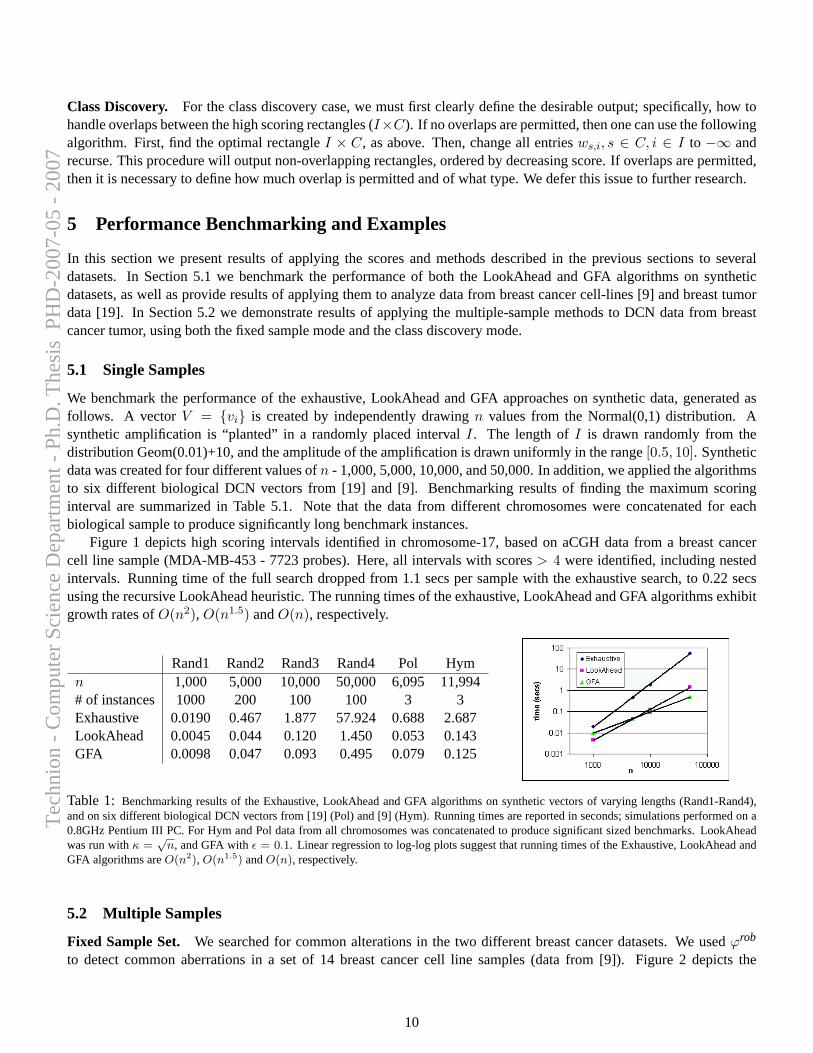
Class Discovery. For the class discovery case, we must first clearly define the desirable output; specifically, how tohandle overlaps between the high scoring rectangles (I×C). If no overlaps are permitted, then one can use the followingalgorithm. First, find the optimal rectangleI × C, as above. Then, change all entriesws,i, s ∈ C, i ∈ I to −∞ andrecurse. This procedure will output non-overlapping rectangles, ordered by decreasing score. If overlaps are permitted,then it is necessary to define how much overlap is permitted and of what type. We defer this issue to further research.
5 Performance Benchmarking and Examples
In this section we present results of applying the scores and methods described in the previous sections to severaldatasets. In Section 5.1 we benchmark the performance of both the LookAhead and GFA algorithms on syntheticdatasets, as well as provide results of applying them to analyze data from breast cancer cell-lines [9] and breast tumordata [19]. In Section 5.2 we demonstrate results of applying the multiple-sample methods to DCN data from breastcancer tumor, using both the fixed sample mode and the class discovery mode.
5.1 Single Samples
We benchmark the performance of the exhaustive, LookAhead and GFA approaches on synthetic data, generated asfollows. A vectorV = {vi} is created by independently drawingn values from the Normal(0,1) distribution. Asynthetic amplification is “planted” in a randomly placed intervalI. The length ofI is drawn randomly from thedistribution Geom(0.01)+10, and the amplitude of the amplification is drawn uniformly in the range[0.5, 10]. Syntheticdata was created for four different values ofn - 1,000, 5,000, 10,000, and 50,000. In addition, we applied the algorithmsto six different biological DCN vectors from [19] and [9]. Benchmarking results of finding the maximum scoringinterval are summarized in Table 5.1. Note that the data from different chromosomes were concatenated for eachbiological sample to produce significantly long benchmark instances.
Figure 1 depicts high scoring intervals identified in chromosome-17, based on aCGH data from a breast cancercell line sample (MDA-MB-453 - 7723 probes). Here, all intervals with scores> 4 were identified, including nestedintervals. Running time of the full search dropped from 1.1 secs per sample with the exhaustive search, to 0.22 secsusing the recursive LookAhead heuristic. The running times of the exhaustive, LookAhead and GFA algorithms exhibitgrowth rates ofO(n2), O(n1.5) andO(n), respectively.
Rand1 Rand2 Rand3 Rand4 Pol Hymn 1,000 5,000 10,000 50,000 6,095 11,994# of instances 1000 200 100 100 3 3Exhaustive 0.0190 0.467 1.877 57.924 0.688 2.687LookAhead 0.0045 0.044 0.120 1.450 0.053 0.143GFA 0.0098 0.047 0.093 0.495 0.079 0.125
Table 1: Benchmarking results of the Exhaustive, LookAhead and GFA algorithms on synthetic vectors of varying lengths (Rand1-Rand4),and on six different biological DCN vectors from [19] (Pol) and [9] (Hym). Running times are reported in seconds; simulations performed on a0.8GHz Pentium III PC. For Hym and Pol data from all chromosomes was concatenated to produce significant sized benchmarks. LookAheadwas run withκ =
√n, and GFA withε = 0.1. Linear regression to log-log plots suggest that running times of the Exhaustive, LookAhead and
GFA algorithms areO(n2), O(n1.5) andO(n), respectively.
5.2 Multiple Samples
Fixed Sample Set. We searched for common alterations in the two different breast cancer datasets. We usedϕrob
to detect common aberrations in a set of 14 breast cancer cell line samples (data from [9]). Figure 2 depicts the
10
Tec
hnio
n -
Com
pute
r Sc
ienc
e D
epar
tmen
t - P
h.D
. The
sis
PH
D-2
007-
05 -
200
7
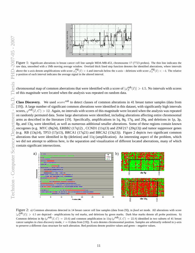
Figure 1: Significant alterations in breast cancer cell line sample MDA-MB-453, chromosome 17 (7723 probes). The thin line indicates theraw data, smoothed with a 1Mb moving average window. Overlaid thick lined step function denotes the identified aberrations, where intervals
above the x-axis denote amplifications with scoreϕsigS (I) > 4 and intervals below the x-axis – deletions with scoreϕ
sigS (I) < −4. The relative
y-position of each interval indicates the average signal in the altered interval.
chromosomal map of common aberrations that were identified with a score of|ϕrobS (I)| > 4.5. No intervals with scores
of this magnitude were located when the analysis was repeated on random data.
Class Discovery. We usedscorerob to detect classes of common alterations in 41 breast tumor samples (data from[19]). A large number of significant common alterations were identified in this dataset, with significantly high intervalsscores,ϕrob(I, C) > 12. Again, no intervals with scores of this magnitude were located when the analysis was repeatedon randomly permuted data. Some large aberrations were identified, including alterations affecting entire chromosomalarms as described in the literature [19]. Specifically, amplifications in 1q, 8q, 17q, and 20q, and deletions in 1p, 3p,8p, and 13q, were identified, as well as numerous additional smaller alterations. Some of these regions contain knownoncogenes (e.g. MYC (8q24), ERBB2 (17q12) , CCND1 (11q13) and ZNF217 (20q13)) and tumor suppressor genes(e.g. RB (13q14), TP53 (17p13), BRCA1 (17q21) and BRCA2 (13q13)). Figure 2 depicts two significant commonalterations that were identified in 8p (deletion) and 11q (amplification). An interesting aspect of the problem, whichwe did not attempt to address here, is the separation and visualization of different located aberrations, many of whichcontain significant intersections.
Figure 2: a) Common alterations detected in 14 breast cancer cell line samples (data from [9]), infixed setmode. All alterations with score
|ϕrobS (I)| > 4.5 are depicted - amplifications by red marks, and deletions by green marks. Dark blue marks denote all probe positions. b)
Common deletion in 8p (ϕrob(I, C) = 23.6) and common amplification in 11q (ϕrob(I, C) = 22.8) identified in two subsets of 41 breastcancer samples inclass discoverymode,τ = 0 (data from [19]). X-axis denotes chromosomal position. Samples are arbitrarily ordered in y-axisto preserve a different class structure for each alteration. Red positions denote positive values and green – negative values.
11
Tec
hnio
n -
Com
pute
r Sc
ienc
e D
epar
tmen
t - P
h.D
. The
sis
PH
D-2
007-
05 -
200
7
References[1] B.R. Balsara and J.R. Testa. Chromosomal imbalances in human lung cancer.Oncogene, 21(45):6877–83, 2002.
[2] Brennan C., Zhang Y., Leo C., Feng B., Cauwels C., Aguirre A.J., Kim M., Protopopov A., and Chin L. High-resolution global profiling ofgenomic alterations with long oligonucleotide microarray.Cancer Research, 64(14):4744–8, 2004.
[3] M.H. DeGroot.Probability and Statistics, chapter 5.7, page 275. Addison-Wesley, 1989.
[4] W. Feller. An Introduction to Probability Theory and Its Applications, volume I, chapter VII.6, page 193. John Wiley & Sons, 1970.
[5] K.S. Fu and J.K. Mui. A survey of image segmentation.Pattern Recognition, 13(1):3–16, 1981.
[6] Bignell G.R., Huang J., Greshock J., Watt S., Butler A., West S., Grigorova M., Jones K.W., Wei W., Stratton M.R., Futreal P.A., WeberB., Shapero M.H., and Wooster R. High-resolution analysis of DNA copy number using oligonucleotide microarrays.Genome Research,14(2):287–95, 2004.
[7] I. Hedenfalk, M. Ringner, A. Ben-Dor, Z. Yakhini, Y. Chen, G. Chebil, R. Ach, N. Loman, H. Olsson, P. Meltzer, A. Borg A, and J. Trent.Molecular classification of familial non-BRCA1/BRCA2 breast cancer.PNAS, 100(5):2532–7, 2003.
[8] J. Himberg, K. Korpiaho, H. Mannila, J. Tikanmki, , and H.T.T. Toivonen. Time series segmentation for context recognition in mobiledevices. InProceedings of the 2001 IEEE International Conference on Data Mining (ICDM 2001), pages 203–210, 2001.
[9] E. Hyman, P. Kauraniemi, S. Hautaniemi, M. Wolf, S. Mousses, E. Rozenblum, M. Ringner, G. Sauter, O. Monni, A. Elkahloun, O.P.Kallioniemi, and A. Kallioniemi. Impact of DNA amplification on gene expression patterns in breast cancer.Cancer Research, 62:6240–5,2002.
[10] Sebat J., Lakshmi B., Troge J., Alexander J., Young J., Lundin P., Maner S., Massa H., Walker M., Chi M., Navin N., Lucito R., Healy J.,Hicks J., Ye K., Reiner A., Gilliam T.C., Trask B., Patterson N., Zetterberg A., and Wigler M. Large-scale copy number polymorphism inthe human genome.Science, 305(5683):525–8, 2004.
[11] O.P. Kallioniemi, A. Kallioniemi, D. Sudar, D. Rutovitz, J.W. Gray, F. Waldman, and D. Pinkel. Comparative genomic hybridization: arapid new method for detecting and mapping DNA amplification in tumors.Semin Cancer Biol, 4(1):41–46, 1993.
[12] D. Lipson, A. Ben-Dor, E. Dehan, and Z. Yakhini. Joint analysis of DNA copy numbers and expression levels. InFourth Workshop onAlgorithms in Bioinformatics (WABI 04), LNCS. Springer, 2004. In press.
[13] Morley M., Molony C.M., Weber T.M., Devlin J.L., Ewens K.G., Spielman R.S., and Cheung V.G. Genetic analysis of genome-widevariation in human gene expression.Nature, 430(7001):743–7, 2004.
[14] F. Mertens, B. Johansson, M. Hoglund, and F. Mitelman. Chromosomal imbalance maps of malignant solid tumors: a cytogenetic surveyof 3185 neoplasms.Cancer Research, 57(13):2765–80, 1997.
[15] Hupe P., Stransky N., Thiery J.P., Radvanyi F., and Barillot E. Analysis of array CGH data: from signal ratio to gain and loss of dna regions.Bioinformatics, 2004. (Epub ahead of print).
[16] D. Pinkel, R. Segraves, D. Sudar, S. Clark, I. Poole, D. Kowbel, C. Collins, W.L. Kuo, C. Chen, Y. Zhai, S.H. Dairkee, B.M. Ljung, J.W.Gray, and D.G. Albertson. High resolution analysis of DNA copy number variation using comparative genomic hybridization to microarrays.Nature Genetics, 20(2):207–211, 1998.
[17] P. Platzer, M.B. Upender, K. Wilson, J. Willis, J. Lutterbaugh, A. Nosrati, J.K. Willson, D. Mack, T. Ried, and S. Markowitz. Silence ofchromosomal amplifications in colon cancer.Cancer Research, 62(4):1134–8, 2002.
[18] J.R. Pollack, C.M. Perou, A.A. Alizadeh, M.B. Eisen, A. Pergamenschikov, C.F. Williams, S.S. Jeffrey, D. Botstein, and P.O. Brown.Genome-wide analysis of DNA copy-number changes using cDNA microarrays.Nature Genetics, 23(1):41–6, 1999.
[19] J.R. Pollack, T. Sorlie, C.M. Perou, C.A. Rees, S.S. Jeffrey, P.E. Lonning, R. Tibshirani, D. Botstein, A. Borresen-Dale, and P.O. Brown.Microarray analysis reveals a major direct role of DNA copy number alteration in the transcriptional program of human breast tumors.PNAS, 99(20):12963–8, 2002.
[20] J. Polzehl and S. Spokoiny. Adaptive weights smoothing with applications to image restoration.J. Royal Statistics Society B, 62:335–354,2000.
12
Tec
hnio
n -
Com
pute
r Sc
ienc
e D
epar
tmen
t - P
h.D
. The
sis
PH
D-2
007-
05 -
200
7

A Proof of Theorem 2.1
Let f : R → R be a strictly concave function (that istf(x) + (1 − t)f(y) < f(tx + (1 − t)y) for all 0 < t < 1).We define the score of an intervalI with respect tof , denotedSf (I), to be the sum ofI ’s entries divided byf(|I|). Inparticular, forf(x) =
√x, S(I) coincides with the interval score function we use throughout this paper.
For a given vector of real numbers, of lengthn, let m > 0 denote the maximal interval score obtained (among all(n2
)intervals). We call an intervaloptimal if its score equalsm. The following theorem bounds the number of optimal
intervals:
Theorem A.1. There can be at mostn optimal intervals.
Claim A.2. For all x, y > z > 0 the following inequality holds:f(x) + f(y) > f(z) + f(x + y − z) Proof. Definet = (x− z)/(x + y − 2z). Note that
x = t(x + y − z) + (1− t)z, and y = tz + (1− t)(x + y − z).
Asf is strictly concave, and0 < t < 1
tf(x + y − z) + (1− t)f(z) < f(t(x + y − z) + (1− t)(z)) = f(x)tf(z) + (1− t)f(x + y − z) < f(t(z) + (1− t)(x + y − z)) = f(y)
Summing the above two inequalities, we get
f(x + y + z) + f(z) < f(x) + f(y)
Claim A.3. If two optimal intervalsI andJ intersect each other than eitherI properly containsJ or vise versa.
Claim A.4. If two optimal intervalsI andJ are disjoint, there must be at least one point between them which is notincluded in either. Otherwise, consider the intervalK = I;J representing their union.
LetI be a collection of optimal intervals. For eachx ∈ {1, . . . , n}we denote byI(x) the set set of optimal intervalsthat containsx.
Claim A.5. All intervals inI(x) have different sizes. Proof. Any two optimal intervals that containsx intersect. ByClaim A.3 one of them properly contains the other. Thus, they have different size.
We define for eachx the smallest interval that containsx, denoted byT (x). Note that by the previous claim, therecan be only one minimal interval that containsx. To complete the upper bound proof, we show now that the mappingT : {1, . . . , n} ← I is onto.
Lemma A.6. For each optimal intervalI there exist a pointx such thatT (x) = I. Proof. LetI be an optimal interval,I = [i,←, j]. We consider two cases
• The leftmost pointi, of I, is not included in any intervalJ ⊂ I. By ClaimA.3 all the intervals that containsi mustcontainI, and thusI is the smallest interval that containsi. ThereforeT (i) = I.
• Otherwise, letJ denote the largest interval that is properly contained inI andi ∈ J . let k denote the rightmostpoint inJ . We show now thatT (k + 1) = I.
First note that sinceJ is properly contained inI, andJ contains the leftmost point ofI, J cannot contain therightmost point ofI. Thereforek + 1 ∈ I. Assume, towards contradiction, that there exist a shorter intervalI ′
that containsk + 1. AsI ′ intersectI and it is shorter, it must be (Claim A.3) properly contained inI. Let i′ ≥ idenote the leftmost point ofI ′. We consider three case
– i′ = i. In this casei ∈ I ′, andJ ⊂ I ′ a contradiction to the definition ofJ .
13
Tec
hnio
n -
Com
pute
r Sc
ienc
e D
epar
tmen
t - P
h.D
. The
sis
PH
D-2
007-
05 -
200
7

– i < i′ ≤ k. In this we contradict Claim A.3 as
k ∈ J ∩ I ′, i ∈ J \ I ′, k + 1 ∈ I ′ \ J.
– i′ = k + 1. In this case,k + 1 is the leftmost point ofI ′, whilek is the leftmost point ofJ , a contradictionto Claim A.4.
Therefore, thereI is the smallest interval containingk + 1, and thusT (k + 1) = I.
We conclude
Theorem A.7. There can be at mostn optimal intervals
This bound is, in fact, tight as can be seen by considering any prefix ofv1 = 1, ...vi = f(i)− f(i− 1), ....
B Algorithm for computing opt(I)
For a MatrixW and an intervalI, the following algorithm efficiently computesopt(I). Note that we assume that foreachs andj, sums([1, j]) is already known. This can be done in a preprocessing phase, for alls andj in O(n|S|).
Algorithm 4 Computingopt(I)Input: Matrix W = {ws,i}, IntervalI = [x, y].Output: opt(I).
Foreachs ∈ S computesums(I) = sums([1, y])− sums([1, x− 1])Sort the values ofsums(I) in decreasing order. Lets1, . . . , sm be the order of thes’s.sum(0) = 0for ` = 1 to m do
sum(`) = sum(`− 1) + sum(I)s`
Outputopt(I) = max`{sum(`)/√
`}
14
Tec
hnio
n -
Com
pute
r Sc
ienc
e D
epar
tmen
t - P
h.D
. The
sis
PH
D-2
007-
05 -
200
7
A.4 Determining the Center of array-CGH
Data
Doron Lipson, Amir Ben-Dor, and Zohar Yakhini. “Determining the Cen-ter of array-CGH Data”. In preparation.
105
Tec
hnio
n -
Com
pute
r Sc
ienc
e D
epar
tmen
t - P
h.D
. The
sis
PH
D-2
007-
05 -
200
7

106
Tec
hnio
n -
Com
pute
r Sc
ienc
e D
epar
tmen
t - P
h.D
. The
sis
PH
D-2
007-
05 -
200
7

BIOINFORMATICS Vol. 00 no. 0 2006, pages 1–5 doi:10.1093/bioinformatics/bti283
Genome analysis
Determining the Center of array-CGH Data Doron Lipson1,*, Amir Ben-Dor2 and Zohar Yakhini1,2
1Department of Computer Science, Technion, Haifa, Israel 2Agilent Laboratories, Santa-Clara, CA, USA
ABSTRACT Motivation: Many statistical and algorithmic approaches to aberra-tion calling in aCGH data are based on the assumption that the data points are distributed around some zero value when no aberration occurs. Currently aCGH data fluorescence ratios are typically nor-malized for each array by setting the average log fluorescence ratio for all array elements to zero. This may lead to erroneous aberration calls for highly-aberrant genomes such as in tumor samples. Results: We present an efficient method for determining the center in array-CGH data. Our method is based on the principle of seeking the simplest explanation of the data – a center postulating a minimal number of aberrations. We apply an implementation of our method, CenterCGH, to a set of aCGH samples from various sources.
1 INTRODUCTION Many genomic and genetic studies are directed to the identification of differences in gene dosage and DNA copy number among cell populations for the purpose of improving the understanding of human disease conditions and the success in correctly diagnosing them. For example, many malignancies involve the gain or loss of DNA sequences (alterations in copy number), sometimes entire chromosomes, that may result in activation of oncogenes or inacti-vation of tumor suppressor genes. The identification of the genetic events leading to neoplastic transformation and subsequent pro-gression can facilitate efforts to define the biological basis for dis-ease, improve prognostication of therapeutic response, and permit earlier tumor detection. In addition, prenatal genetic problems frequently result from loss or gain of chromosome segments (such as trisomy 21).
Comparative genomic hybridization (CGH) is a technique that is used to evaluate variations in genomic copy number in cells. In the classical version of CGH, genomic DNA is isolated from normal reference cells, as well as from test cells (e.g., tumor cells). The two nucleic acids are differentially labeled and then simultaneously hybridized in situ to metaphase chromosomes of a reference cell. Chromosomal regions in the test cells which are at increased or decreased copy number can be identified by detecting regions where the ratio of signal from the two distinguishably labeled nu-cleic acids is altered (Kallioniemi et al, 1993). In further technol-ogy development the metaphase chromosomes are replaced by microarrays with probes that represent the genome. Pinkel et al (1998) used BAC probes to measure changes in DNA copy num-bers for human breast tumor samples. Pollack et al (1999) used cDNA array to measure gene copy changes in similar specimens. Recent technology developments introduced oligonucleotide array platforms for array based comparative genomic hybridization (aCGH) analyses (Bignell et al, 2004, Brennan et al, 2004, Barrett et al, 2004). One of the major advantages of the oligonucleotide array platform is that oligonucleotide probes can be designed in
silico for any sequenced region, coding and non-coding), of a ge-nome of interest.
To fully realize the advantages associated with the emerging high resolution technologies, practitioners need appropriate effi-cient data analysis methods. A common first step in analyzing DNA copy number data consists of identifying aberrant (amplified or deleted) regions in each individual sample. aCGH yields data that can be represented as a vector of log-ratio values associated with the genomic location of the probe at which they were meas-ured.
Several statistical and algorithmic approaches to aberration call-ing are described in the literature. Some of these approaches em-ploy a two-stage process – first the data vector is segmented and then the segments are designated as aberrant or not. An example of this two-stage approach is the Circular Binary Segmentation method (Olshen et al, 2004) as well as in a recent review study (Lai et al, 2005). Other approaches such as using HMMs (Fridly-and et al, 2004) or optimizing a statistical score that measure aber-rations (Lipson et al, 2005) identify aberrant and non-aberrant intervals in one stage and therefore jointly perform the segmenta-tion and the statistical calling.
The basis for assigning a statistical aberration score to an inter-val involves, whether in a two-stage or in a one-stage approach, assuming a zero value for the data – the mean around which we expect the data to be distributed when no aberration occurred. Cur-rently aCGH data fluorescence ratios are typically normalized for each array by setting the average log fluorescence ratio for all array elements to zero. For illustration, consider a male vs female aCGH assay. As all probes residing on chromosome X are expected to yield a non-zero log fluorescence ratio and as all other probes are expected to yield signals centered around zero we don’t, in fact, expect the normalization above to yield a value that represents the real center of the diploid part of the sample. In this case, it is easy to overcome the problem by excluding the X chromosome from the centralization process, but in most cases the aberrant regions of the genome are not well defined a-priori. The purpose of the methods described in this paper is to provide a more sound approach to identifying that center.
The task of identifying the zero in aCGH data is important since aberration-calling statistics can be affected by differences in this value. Fig 1 describes aCGH data from the entire genome of the human breast cancer cell-line T47D, measured on cDNA arrays (Pollack et al, 2002). Two sets of identified aberrations are de-picted, as determined by the algorithm Stepgram (Lipson et al, 2005). The first is under the null assumption of signals normally distributed centered around the 0 (as determined by the average log normalization scheme) and the second, simpler one, is obtained under the null assumption that signals are centered at ζ = -0.26.
This exemplifies the principle followed by the methods pre-sented here – map the center of the aCGH data vector to a value that yields the simplest explanation of the data – the one postulat-
© Oxford University Press 2005 1
Tec
hnio
n -
Com
pute
r Sc
ienc
e D
epar
tmen
t - P
h.D
. The
sis
PH
D-2
007-
05 -
200
7
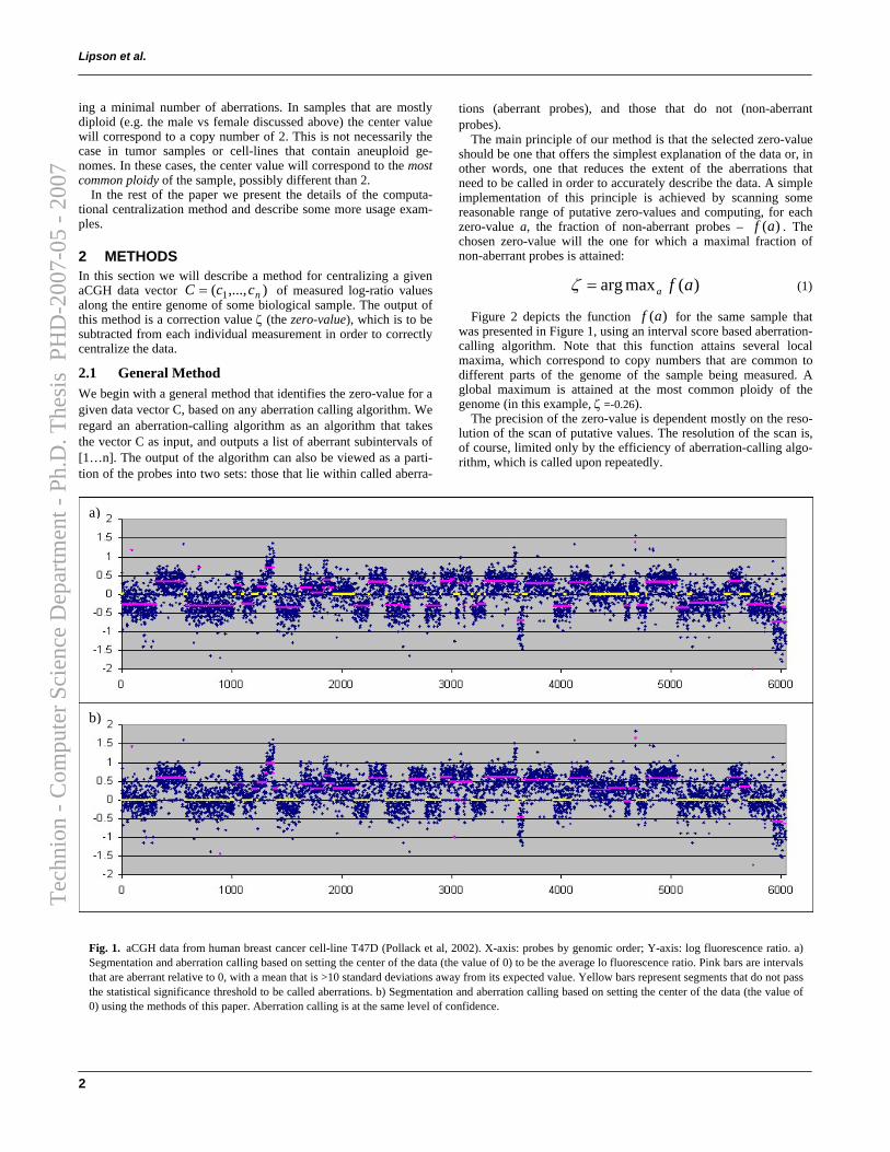
Lipson et al.
ing a minimal number of aberrations. In samples that are mostly diploid (e.g. the male vs female discussed above) the center value will correspond to a copy number of 2. This is not necessarily the case in tumor samples or cell-lines that contain aneuploid ge-nomes. In these cases, the center value will correspond to the most common ploidy of the sample, possibly different than 2.
In the rest of the paper we present the details of the computa-tional centralization method and describe some more usage exam-ples.
2 METHODS In this section we will describe a method for centralizing a given aCGH data vector of measured log-ratio values along the entire genome of some biological sample. The output of this method is a correction value ζ (the zero-value), which is to be subtracted from each individual measurement in order to correctly centralize the data.
),...,( 1 nccC =
2.1 General Method We begin with a general method that identifies the zero-value for a given data vector C, based on any aberration calling algorithm. We regard an aberration-calling algorithm as an algorithm that takes the vector C as input, and outputs a list of aberrant subintervals of [1…n]. The output of the algorithm can also be viewed as a parti-tion of the probes into two sets: those that lie within called aberra-
tions (aberrant probes), and those that do not (non-aberrant probes).
The main principle of our method is that the selected zero-value should be one that offers the simplest explanation of the data or, in other words, one that reduces the extent of the aberrations that need to be called in order to accurately describe the data. A simple implementation of this principle is achieved by scanning some reasonable range of putative zero-values and computing, for each zero-value a, the fraction of non-aberrant probes – . The chosen zero-value will the one for which a maximal fraction of non-aberrant probes is attained:
)(af
)(maxarg afa=ζ (1)
Figure 2 depicts the function for the same sample that was presented in Figure 1, using an interval score based aberration-calling algorithm. Note that this function attains several local maxima, which correspond to copy numbers that are common to different parts of the genome of the sample being measured. A global maximum is attained at the most common ploidy of the genome (in this example, ζ =-0.26).
)(af
The precision of the zero-value is dependent mostly on the reso-lution of the scan of putative values. The resolution of the scan is, of course, limited only by the efficiency of aberration-calling algo-rithm, which is called upon repeatedly.
Fig. 1. aCGH data from human breast cancer cell-line T47D (Pollack et al, 2002). X-axis: probes by genomic order; Y-axis: log fluorescence ratio. a) Segmentation and aberration calling based on setting the center of the data (the value of 0) to be the average lo fluorescence ratio. Pink bars are intervals that are aberrant relative to 0, with a mean that is >10 standard deviations away from its expected value. Yellow bars represent segments that do not pass the statistical significance threshold to be called aberrations. b) Segmentation and aberration calling based on setting the center of the data (the value of 0) using the methods of this paper. Aberration calling is at the same level of confidence.
b)
a)
2
Tec
hnio
n -
Com
pute
r Sc
ienc
e D
epar
tmen
t - P
h.D
. The
sis
PH
D-2
007-
05 -
200
7
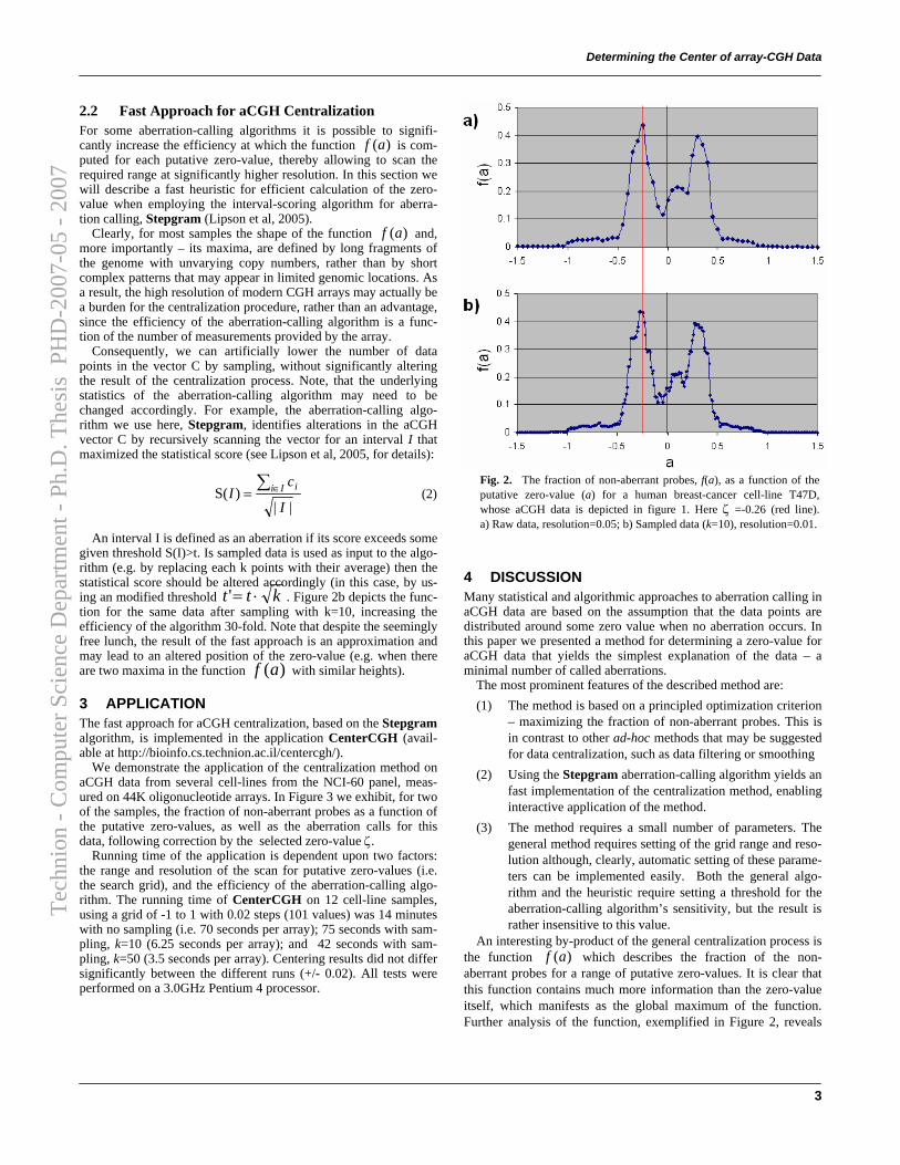
Determining the Center of array-CGH Data
2.2 Fast Approach for aCGH Centralization For some aberration-calling algorithms it is possible to signifi-cantly increase the efficiency at which the function is com-puted for each putative zero-value, thereby allowing to scan the required range at significantly higher resolution. In this section we will describe a fast heuristic for efficient calculation of the zero-value when employing the interval-scoring algorithm for aberra-tion calling, Stepgram (Lipson et al, 2005).
)(af
Clearly, for most samples the shape of the function and, more importantly – its maxima, are defined by long fragments of the genome with unvarying copy numbers, rather than by short complex patterns that may appear in limited genomic locations. As a result, the high resolution of modern CGH arrays may actually be a burden for the centralization procedure, rather than an advantage, since the efficiency of the aberration-calling algorithm is a func-tion of the number of measurements provided by the array.
)(af
Consequently, we can artificially lower the number of data points in the vector C by sampling, without significantly altering the result of the centralization process. Note, that the underlying statistics of the aberration-calling algorithm may need to be changed accordingly. For example, the aberration-calling algo-rithm we use here, Stepgram, identifies alterations in the aCGH vector C by recursively scanning the vector for an interval I that maximized the statistical score (see Lipson et al, 2005, for details):
||
)S(I
cI Ii i∑∈= (2)
Fig. 2. The fraction of non-aberrant probes, f(a), as a function of the
An interval I is defined as an aberration if its score exceeds some given threshold S(I)>t. Is sampled data is used as input to the algo-rithm (e.g. by replacing each k points with their average) then the statistical score should be altered accordingly (in this case, by us-ing an modified threshold ktt ⋅=' . Figure 2b depicts the func-tion for the same data after sampling with k=10, increasing the efficiency of the algorithm 30-fold. Note that despite the seemingly free lunch, the result of the fast approach is an approximation and may lead to an altered position of the zero-value (e.g. when there are two maxima in the function with similar heights). )(af
3 APPLICATION The fast approach for aCGH centralization, based on the Stepgram algorithm, is implemented in the application CenterCGH (avail-able at http://bioinfo.cs.technion.ac.il/centercgh/).
We demonstrate the application of the centralization method on aCGH data from several cell-lines from the NCI-60 panel, meas-ured on 44K oligonucleotide arrays. In Figure 3 we exhibit, for two of the samples, the fraction of non-aberrant probes as a function of the putative zero-values, as well as the aberration calls for this data, following correction by the selected zero-value ζ.
Running time of the application is dependent upon two factors: the range and resolution of the scan for putative zero-values (i.e. the search grid), and the efficiency of the aberration-calling algo-rithm. The running time of CenterCGH on 12 cell-line samples, using a grid of -1 to 1 with 0.02 steps (101 values) was 14 minutes with no sampling (i.e. 70 seconds per array); 75 seconds with sam-pling, k=10 (6.25 seconds per array); and 42 seconds with sam-pling, k=50 (3.5 seconds per array). Centering results did not differ significantly between the different runs (+/- 0.02). All tests were performed on a 3.0GHz Pentium 4 processor.
4 DISCUSSION Many statistical and algorithmic approaches to aberration calling in aCGH data are based on the assumption that the data points are distributed around some zero value when no aberration occurs. In this paper we presented a method for determining a zero-value for aCGH data that yields the simplest explanation of the data – a minimal number of called aberrations.
The most prominent features of the described method are: (1) The method is based on a principled optimization criterion
– maximizing the fraction of non-aberrant probes. This is in contrast to other ad-hoc methods that may be suggested for data centralization, such as data filtering or smoothing
(2) Using the Stepgram aberration-calling algorithm yields an fast implementation of the centralization method, enabling interactive application of the method.
(3) The method requires a small number of parameters. The general method requires setting of the grid range and reso-lution although, clearly, automatic setting of these parame-ters can be implemented easily. Both the general algo-rithm and the heuristic require setting a threshold for the aberration-calling algorithm’s sensitivity, but the result is rather insensitive to this value.
An interesting by-product of the general centralization process is the function which describes the fraction of the non-aberrant probes for a range of putative zero-values. It is clear that this function contains much more information than the zero-value itself, which manifests as the global maximum of the function. Further analysis of the function, exemplified in Figure 2, reveals
)(af
putative zero-value (a) for a human breast-cancer cell-line T47D, whose aCGH data is depicted in figure 1. Here ζ =-0.26 (red line). a) Raw data, resolution=0.05; b) Sampled data (k=10), resolution=0.01.
3
Tec
hnio
n -
Com
pute
r Sc
ienc
e D
epar
tmen
t - P
h.D
. The
sis
PH
D-2
007-
05 -
200
7
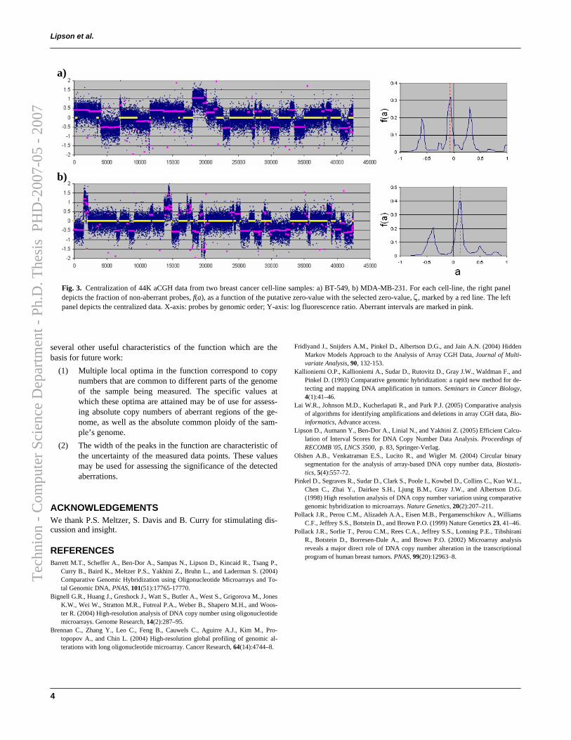
Lipson et al.
4
Fig. 3. Centralization of 44K aCGH data from two breast cancer cell-line samples: a) BT-549, b) MDA-MB-231. For each cell-line, the right panel depicts the fraction of non-aberrant probes, f(a), as a function of the putative zero-value with the selected zero-value, ζ, marked by a red line. The left panel depicts the centralized data. X-axis: probes by genomic order; Y-axis: log fluorescence ratio. Aberrant intervals are marked in pink.
a)
b)
several other useful characteristics of the function which are the basis for future work:
(1) Multiple local optima in the function correspond to copy numbers that are common to different parts of the genome of the sample being measured. The specific values at which these optima are attained may be of use for assess-ing absolute copy numbers of aberrant regions of the ge-nome, as well as the absolute common ploidy of the sam-ple’s genome.
(2) The width of the peaks in the function are characteristic of the uncertainty of the measured data points. These values may be used for assessing the significance of the detected aberrations.
ACKNOWLEDGEMENTS We thank P.S. Meltzer, S. Davis and B. Curry for stimulating dis-cussion and insight.
REFERENCES Barrett M.T., Scheffer A., Ben-Dor A., Sampas N., Lipson D., Kincaid R., Tsang P.,
Curry B., Baird K., Meltzer P.S., Yakhini Z., Bruhn L., and Laderman S. (2004) Comparative Genomic Hybridization using Oligonucleotide Microarrays and To-tal Genomic DNA, PNAS, 101(51):17765-17770.
Bignell G.R., Huang J., Greshock J., Watt S., Butler A., West S., Grigorova M., Jones K.W., Wei W., Stratton M.R., Futreal P.A., Weber B., Shapero M.H., and Woos-ter R. (2004) High-resolution analysis of DNA copy number using oligonucleotide microarrays. Genome Research, 14(2):287–95.
Brennan C., Zhang Y., Leo C., Feng B., Cauwels C., Aguirre A.J., Kim M., Pro-topopov A., and Chin L. (2004) High-resolution global profiling of genomic al-terations with long oligonucleotide microarray. Cancer Research, 64(14):4744–8.
Fridlyand J., Snijders A.M., Pinkel D., Albertson D.G., and Jain A.N. (2004) Hidden Markov Models Approach to the Analysis of Array CGH Data, Journal of Multi-variate Analysis, 90, 132-153.
Kallioniemi O.P., Kallioniemi A., Sudar D., Rutovitz D., Gray J.W., Waldman F., and Pinkel D. (1993) Comparative genomic hybridization: a rapid new method for de-tecting and mapping DNA amplification in tumors. Seminars in Cancer Biology, 4(1):41–46.
Lai W.R., Johnson M.D., Kucherlapati R., and Park P.J. (2005) Comparative analysis of algorithms for identifying amplifications and deletions in array CGH data, Bio-informatics, Advance access.
Lipson D., Aumann Y., Ben-Dor A., Linial N., and Yakhini Z. (2005) Efficient Calcu-lation of Interval Scores for DNA Copy Number Data Analysis. Proceedings of RECOMB '05, LNCS 3500, p. 83, Springer-Verlag.
Olshen A.B., Venkatraman E.S., Lucito R., and Wigler M. (2004) Circular binary segmentation for the analysis of array-based DNA copy number data, Biostatis-tics, 5(4):557-72.
Pinkel D., Segraves R., Sudar D., Clark S., Poole I., Kowbel D., Collins C., Kuo W.L., Chen C., Zhai Y., Dairkee S.H., Ljung B.M., Gray J.W., and Albertson D.G. (1998) High resolution analysis of DNA copy number variation using comparative genomic hybridization to microarrays. Nature Genetics, 20(2):207–211.
Pollack J.R., Perou C.M., Alizadeh A.A., Eisen M.B., Pergamenschikov A., Williams C.F., Jeffrey S.S., Botstein D., and Brown P.O. (1999) Nature Genetics 23, 41–46.
Pollack J.R., Sorlie T., Perou C.M., Rees C.A., Jeffrey S.S., Lonning P.E., Tibshirani R., Botstein D., Borresen-Dale A., and Brown P.O. (2002) Microarray analysis reveals a major direct role of DNA copy number alteration in the transcriptional program of human breast tumors. PNAS, 99(20):12963–8.
Tec
hnio
n -
Com
pute
r Sc
ienc
e D
epar
tmen
t - P
h.D
. The
sis
PH
D-2
007-
05 -
200
7

A.5 Framework for Identifying Common Aber-
rations in DNA Copy Number Data
Amir Ben-Dor, Doron Lipson, Anya Tsalenko, Mark Reimers, Lars O. Baum-busch, Michael T. Barrett, John N. Weinstein, Anne-Lise Borresen-Dale, andZohar Yakhini, “Framework for Identifying Common Aberrations inDNA Copy Number Data”. Accepted for presentation at RECOMB ’07.
111
Tec
hnio
n -
Com
pute
r Sc
ienc
e D
epar
tmen
t - P
h.D
. The
sis
PH
D-2
007-
05 -
200
7

112
Tec
hnio
n -
Com
pute
r Sc
ienc
e D
epar
tmen
t - P
h.D
. The
sis
PH
D-2
007-
05 -
200
7
Framework for Identifying Common Aberrationsin DNA Copy Number Data
Amir Ben-Dor1,�, Doron Lipson2, Anya Tsalenko1, Mark Reimers3,Lars O. Baumbusch4, Michael T. Barrett1,5, John N. Weinstein3,
Anne-Lise Borresen-Dale4, and Zohar Yakhini1,2
1 Agilent Laboratories, Santa-Clara, CA2 Computer Science Dept., Technion, Haifa3 National Cancer Institute, Bethesda, MD
4 Department of Genetics, Institute for Cancer Research,Rikshospitalet-Radiumhospitalet Medical Center
5 Translational Genomics Research Institute, Phoenix, AZamir [email protected]
Abstract. High-resolution array comparative genomic hybridization(aCGH) provides exon-level mapping of DNA aberrations in cells or tis-sues. Such aberrations are central to carcinogenesis and, in many cases,central to targeted therapy of the cancers. Some of the aberrations aresporadic, one-of-a-kind changes in particular tumor samples; others oc-cur frequently and reflect common themes in cancer biology that haveinterpretable, causal ramifications. Hence, the difficult task of identify-ing and mapping common, overlapping genomic aberrations (includingamplifications and deletions) across a sample set is an important one; itcan provide insight for the discovery of oncogenes, tumor suppressors,and the mechanisms by which they drive cancer development.
In this paper we present an efficient computational framework foridentification and statistical characterization of genomic aberrations thatare common to multiple cancer samples in a CGH data set. We presentand compare three different algorithmic approaches within the contextof that framework. Finally, we apply our methods to two datasets – acollection of 20 breast cancer samples and a panel of 60 diverse humantumor cell lines (the NCI-60). Those analyses identified both known andnovel common aberrations containing cancer-related genes. The potentialimpact of the analytical methods is well demonstrated by new insightsinto the patterns of deletion of CDKN2A (p16), a tumor suppressor genecrucial for the genesis of many types of cancer.
Keywords: CGH, cancer, microarray data analysis, common aberra-tions, breast cancer, NCI-60.
1 Introduction
Alterations in DNA copy number are characteristic of many cancer types and drivesome cancer pathogenesis processes as well as several developmental disorders.� Corresponding author.
T. Speed and H. Huang (Eds.): RECOMB 2007, LNBI 4453, pp. 122–136, 2007.c© Springer-Verlag Berlin Heidelberg 2007
Tec
hnio
n -
Com
pute
r Sc
ienc
e D
epar
tmen
t - P
h.D
. The
sis
PH
D-2
007-
05 -
200
7
Framework for Identifying Common Aberrations 123
These alterations include large chromosomal gains and losses as well as smallerscale amplifications and deletions. Genomic instability can often trigger the over-expression or activation of oncogenes and the silencing of tumor suppressors.Mapping regions of common genomic aberrations can therefore provide insight tocancer pathogenesis and lead to discovery of cancer-related genes and the mecha-nisms by which they drive the disease. Genomic aberrations are also routinely usedfor diagnosis and clinical practice. For example,Erbb2amplification is a strong pre-dictor of Herceptin activity in breast cancer patients [1]. Similarly, amplificationsof MDM2 and CDK4 genes on chromosome 12q13-15 are useful in distinguishingwell-differentiated liposarcomas from benign adipose tumors [2].
Technologies for measuring alterations in DNA copy number include localfluorescence in situ hybridization-based techniques, Comparative Genomic Hy-bridization (CGH [3,4,5]) and the advanced method termed array CGH (aCGH).In aCGH differentially labeled tumor and normal DNA are co-hybridized to a mi-croarray of thousands to hundreds of thousands of genomic BAC clones, cDNA oroligonucleotide probes [6,7,8,9,10,11,12]. The use of oligonucleotide aCGH allowsthe determination of changes in DNA copy number of relatively small chromo-somal regions. Using high density arrays allows very high DNA copy numberresolution, in terms of genomic distances, down to single Kb and less.
A common first step in analyzing DNA copy number alterations (CNAs) dataconsists of identifying aberrant (amplified or deleted) regions in each individualsample. Aberration calling is the subject of extensive literature [13,14,15,16,17].We briefly address this step of the process in Section 2.1.
To realize the full power of multi-sample, high-resolution oligo-aCGH studies,we are interested in efficient computational methods that enable the automaticelucidation of more complex structures. The focus of this paper is the discov-ery of common genomic aberrations, either in a fixed set of samples or in asignificant subset of the samples. To date, little attention has been given inthe literature to formal treatments of this task. Two important exceptions arethe work of Disking et al [18] and Rouveirol et al [19]. In [18] the authors devel-oped a method called Significance Testing for Aberrant Copy number (STAC) toaddress the detection of DNA copy number aberrations across multiple aCGHexperiments. STAC uses two complementary statistical scores in combinationwith a heuristic search strategy. The significance of both statistics is assessed,and p-values are assigned to each location in the genome by using a permuta-tion approach. In the work of Rouveirol et al [19] the authors propose a formalframework for the task of detecting commonly aberrant regions in CGH data,and present two algorithms (MAR and CMAR) for this task. The frameworkrequires, however, a segmentation algorithm that categorize each data point asbeing gained/lost/normal. Therefore, this approach requires setting an arbitrarythreshold for the discretization step, and is not sensitive to the actual copy num-ber change. In addition, the methods of Lipson et al [20], based on optimizinga statistically motivated score function for genomic intervals can be adapted toautomatic identification of aberrations that are common in subsets of the sam-ple set. Despite the lack of formal approaches to identifying common aberrations
Tec
hnio
n -
Com
pute
r Sc
ienc
e D
epar
tmen
t - P
h.D
. The
sis
PH
D-2
007-
05 -
200
7
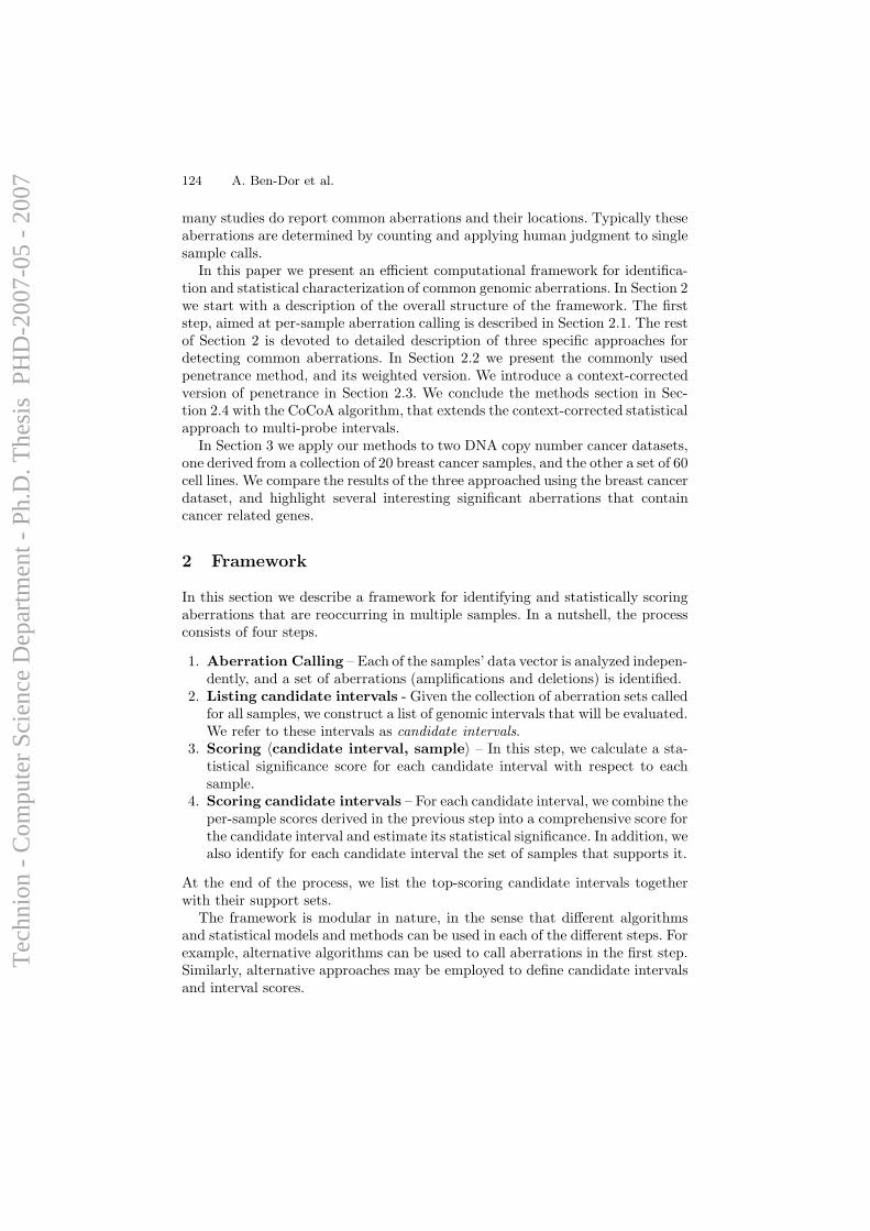
124 A. Ben-Dor et al.
many studies do report common aberrations and their locations. Typically theseaberrations are determined by counting and applying human judgment to singlesample calls.
In this paper we present an efficient computational framework for identifica-tion and statistical characterization of common genomic aberrations. In Section 2we start with a description of the overall structure of the framework. The firststep, aimed at per-sample aberration calling is described in Section 2.1. The restof Section 2 is devoted to detailed description of three specific approaches fordetecting common aberrations. In Section 2.2 we present the commonly usedpenetrance method, and its weighted version. We introduce a context-correctedversion of penetrance in Section 2.3. We conclude the methods section in Sec-tion 2.4 with the CoCoA algorithm, that extends the context-corrected statisticalapproach to multi-probe intervals.
In Section 3 we apply our methods to two DNA copy number cancer datasets,one derived from a collection of 20 breast cancer samples, and the other a set of 60cell lines. We compare the results of the three approached using the breast cancerdataset, and highlight several interesting significant aberrations that containcancer related genes.
2 Framework
In this section we describe a framework for identifying and statistically scoringaberrations that are reoccurring in multiple samples. In a nutshell, the processconsists of four steps.
1. Aberration Calling – Each of the samples’ data vector is analyzed indepen-dently, and a set of aberrations (amplifications and deletions) is identified.
2. Listing candidate intervals - Given the collection of aberration sets calledfor all samples, we construct a list of genomic intervals that will be evaluated.We refer to these intervals as candidate intervals.
3. Scoring 〈candidate interval, sample〉 – In this step, we calculate a sta-tistical significance score for each candidate interval with respect to eachsample.
4. Scoring candidate intervals – For each candidate interval, we combine theper-sample scores derived in the previous step into a comprehensive score forthe candidate interval and estimate its statistical significance. In addition, wealso identify for each candidate interval the set of samples that supports it.
At the end of the process, we list the top-scoring candidate intervals togetherwith their support sets.
The framework is modular in nature, in the sense that different algorithmsand statistical models and methods can be used in each of the different steps. Forexample, alternative algorithms can be used to call aberrations in the first step.Similarly, alternative approaches may be employed to define candidate intervalsand interval scores.
Tec
hnio
n -
Com
pute
r Sc
ienc
e D
epar
tmen
t - P
h.D
. The
sis
PH
D-2
007-
05 -
200
7
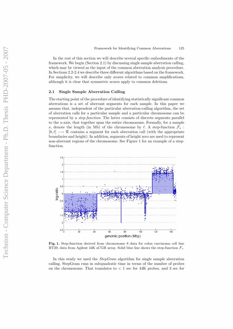
Framework for Identifying Common Aberrations 125
In the rest of this section we will describe several specific embodiments of theframework. We begin (Section 2.1) by discussing single sample aberration calling,which may be viewed as the input of the common aberration analysis procedure.In Sections 2.2-2.4 we describe three different algorithms based on the framework.For simplicity, we will describe only scores related to common amplifications,although it is clear that symmetric scores apply to common deletions.
2.1 Single Sample Aberration Calling
The starting point of the procedure of identifying statistically significant commonaberrations is a set of aberrant segments for each sample. In this paper weassume that, independent of the particular aberration-calling algorithm, the setof aberration calls for a particular sample and a particular chromosome can berepresented by a step-function. The latter consists of discrete segments parallelto the x-axis, that together span the entire chromosome. Formally, for a samples, denote the length (in Mb) of the chromosome by �. A step-function Fs :[0, �] −→ R contains a segment for each aberration call (with the appropriateboundaries and height). In addition, segments of height zero are used to representnon-aberrant regions of the chromosome. See Figure 1 for an example of a step-function.
Fig. 1. Step-function derived from chromosome 8 data for colon carcinoma cell lineHT29, data from Agilent 44K aCGH array. Solid blue line shows the step-function Fs.
In this study we used the StepGram algorithm for single sample aberrationcalling. StepGram runs in subquadratic time in terms of the number of probeson the chromosome. That translates to < 1 sec for 44K probes, and 3 sec for
Tec
hnio
n -
Com
pute
r Sc
ienc
e D
epar
tmen
t - P
h.D
. The
sis
PH
D-2
007-
05 -
200
7
126 A. Ben-Dor et al.
185K probes with current the implementation. StepGram is therefore particu-larly suitable for analysis of large datasets and useful in the context of lookingfor common aberrations. The details of StepGram were described previously byLipson et al [20], and an overview is provided here for completeness.
StepGram. Given a vector of real values V = (v1, . . . , vn) (corresponding tonormalized log-ratio measurements along a particular chromosome) the opti-mization problem solved by StepGram involves identifying the interval I ⊆ [1, n]that maximizes the score |
∑i∈I vi/
√I|. A branch-and-bound approach allows
solving this problem in O(n1.5) time complexity in practice. Following identifica-tion of the maximal scoring interval the analysis is repeated by recursion to theleft, to the right, and within the identified interval until some lower thresholdscore is attained. A stand-alone implementation of the StepGram algorithm ispublicly available at http://bioinfo.cs.technion.ac.il/stepgram/.
Other aberration-calling algorithms. Several other algorithms for identifyingaberrations in DNA copy number data have been described. These include CBS[15] based on binary segmentation, CLAC [16] based on clustering, aCGH [13]based on HMM, ACE [21] based on FDR, and others. Comparison studies ofseveral of these algorithms were conducted by Lai et al [14] and by Willenbrocket al [17]. Note that many of them are segmentation algorithms in the sense thatthey partition the chromosome into segments of equal copy number but do notattempt to identify which of those segments are aberrant. For the purpose ofidentifying common aberrations the segmentation output is typically sufficient.
2.2 Weighted and Unweighted Penetrance
We begin by describing the commonly-used penetrance score and its role withinthe common aberrations analysis framework. Although the penetrance score isnot a measure of statistical significance, it does exemplify the different steps ofthe process.
Candidate intervals. In the case of the penetrance score, the candidate intervalsare defined simply as the positions of the probes in the aCGH array. Similardefinitions, such as uniformly-spaced pseudo-probes, are also possible. In eithercase, for a particular chromosome the candidate intervals can be formally definedas a set of non-overlapping intervals I = {[xi − ε, xi + ε]}. Here ε is an arbitraryconstant smaller then the minimum distance between any two probes on thearray.
Scoring 〈interval, sample〉. For a given interval I = [xi − ε, xi + ε] and samples the unweighted amplification penetrance score is defined as a binary scoreα(I, s) = 1Fs(xi)>t for some threshold t. The weighted penetrance scores takeinto account also the height of the aberration: α′(I, s) = 1Fs(xi)>t · Fs(xi).
Scoring candidate intervals. The overall penetrance score for a given candidateinterval I is defined simply as α(I) =
∑s α(I, s). As noted before, this score
does not reflect any measure of statistical significance.
Tec
hnio
n -
Com
pute
r Sc
ienc
e D
epar
tmen
t - P
h.D
. The
sis
PH
D-2
007-
05 -
200
7

Framework for Identifying Common Aberrations 127
2.3 Context-Corrected Penetrance
A variant of the penetrance score provides a measure of statistical significance ofthe common aberration at the specified probe. The significance is defined withrespect to the genomic background of each sample, as represented by the patternof aberrations over each of the samples. In other words, given the specific set ofaberration calls for each sample, we wish to describe our “surprise” at seeing aspecific set of aberrations co-localized at the same genomic position. Note thatthe context provided for the score may be either genomic or chromosomal.
Candidate intervals. As was in the case of the penetrance score, the candidateintervals are defined as as a set of non-overlapping intervals at specific genomicpositions: I = {[xi − ε, xi + ε]}.
Scoring 〈interval, sample〉. For the context-corrected score, we wish the scoreof a given interval I = [xi − ε, xi + ε] and sample s to reflect the probabilityof finding an interval of similar (or higher) amplitude given the context of thesample. The score is therefore defined as
p(I, s) =|{xj ∈ I : Fs(xj) ≥ Fs(xi)}|
|I| .
Scoring candidate intervals. Let S be the set of samples, with m = |S|. Fora given interval I we now have m scores. Note that the interval I might beaberrant in only a subset of the samples, we therefore seek the subset of samplesthat will provide maximal significance. Assume, w.l.o.g., that p(I, 1) ≤ p(I, 2) ≤. . . ≤ p(I, m). Looking at the first k samples, the probability of concurrentlyobserving k or more scores of probability p = p(I, k) or lower is provided by theBinomial distribution:
ρk(I) = Binom(k, m, p) =m∑
i=k
(m
i
)
pi(1 − p)m−i
Since we are interested in identifying aberrations that occur in at least twosamples, and to address multiple testing concerns, we define a more conservativescore that ignores the first success in the computation,
ρ′
k(I) = Binom(k − 1, m − 1, p)
We define the score of I, to be the minimum of these scores over all values of k,namely,
ρ(I) = mink=1,...,m−1
ρ′
k(I).
2.4 Context-Corrected Common Aberrations (CoCoA)
Although the context-corrected penetrance algorithm will clearly detect statisti-cally significant common aberrations that are affecting a single probe, its ability
Tec
hnio
n -
Com
pute
r Sc
ienc
e D
epar
tmen
t - P
h.D
. The
sis
PH
D-2
007-
05 -
200
7
128 A. Ben-Dor et al.
to detect larger significant aberrations is not guaranteed. In some cases, a multi-probe common aberration may be significant as a whole, although the score ofeach single probe contained in the aberration may not show statistical signifi-cance. For example, consider the case in which each of many samples containsmany random high-amplitude single-probe amplifications and a common largemoderate-amplitude amplification. In that case, the size of the aberration mayhelp us to determine its significance, since not many random aberrations of thesame size will be detected in the background.
The third, most sophisticated, algorithm for identifying significant commonaberrations expands the concept of a context-corrected significance score to in-tervals that are larger than a single probe.
Candidate intervals. Consider a particular chromosome, c, and denote by T ={[b1, e1], . . . , [bk, ek]} the set of all genomic intervals in c that are called as aber-rant in any of the samples. The set of candidate intervals in c is defined to be allgenomic intervals that starts at the left side of one interval from T and end atthe right side of another. That is, I = {[bi, ej ] : 1 ≤ i, j ≤ k, and bi ≤ ej}. Notethat the size of I is quadratic in k, the number of called aberrations. A smallerlist of candidate intervals can be constructed by considering only intervals in Tand intersections thereof. that is I = T ∪ {t ∩ s : t, s ∈ T }. The size of I istypically o(k2), and can be constructed in linear time (proof omitted).
Scoring 〈interval, sample〉. Applying the same reasoning as for the Context-Corrected Penetrance, we wish the score of a given interval I = [b, e] and samples to reflect the probability of finding an interval of the same length with a similar(or higher) amplitude given the context of the sample. More specifically, assumewe pick a random interval J of the same size as I in the context (that is, inthe same chromosome, or in the entire genome). The score is defined as theprobability that the average height of J would be as high (or higher) as theheight of I,
p(I, s) = PrJ:|J|=|I| (hs(J) ≥ hs(I)) .
where |I| denotes the genomic size I, and hs(J) denotes the average height of thestep-function Fs over the interval J . We outline now how to computed p(I, s)efficiently (in linear time). Denote by Fs,�(·) the �-window moving average ofFs. The score p(I, s), can now be expressed as a function of Fs,�,
p(I, s) =|x : Fs,�(x) ≥ hs(I)|
c − �.
where c denoted the length of the chromosome. Since Fs is a step-function,its moving average Fs,� is a piecewise-linear function. Thus, we can efficientlyidentify the regions where Fs,�(x) ≥ hs(i), and compute p(I, s).
Scoring candidate intervals. After computing context-corrected per-samplescores for I, we combine them into a statistical score for I using the same bino-mial distribution calculation as detailed in Section 2.3.
Tec
hnio
n -
Com
pute
r Sc
ienc
e D
epar
tmen
t - P
h.D
. The
sis
PH
D-2
007-
05 -
200
7
Framework for Identifying Common Aberrations 129
3 Results
In this section we demonstrate the application of the above methods to DNAcopy number data from two datasets, both measured using Agilent 44K aCGHarrays:
1. A set of 20 primary breast tumor samples were included in this study. Thesesamples are part of a larger patient cohort consisting of 920 breast cancerpatients stage I and II referred for surgical treatment and where detection ofisolated tumor cells in bone marrow was performed (The Oslo Micrometas-tases Study) [22]. Tumor material were fresh frozen immediately after surgeryand stored at -80C until use. Although the sample set includes several dis-tinct subtypes that had previously been characterized [23,24], due to itsrelative homogeneity, we expected to encounter common aberrations typicalof breast cancer.
2. A diverse set of 60 cancer cell-lines known as the NCI-60 cell line panel [25].The NCI-60 panel has been used by the Developmental Therapeutics Pro-gram (DTP) of the U.S. National Cancer Institute (NCI) to screen > 100, 000chemical compounds and natural product extracts for anticancer activitysince 1990 [26,27,25]. The NCI-60 panel is comprised of cell lines from di-verse human cancers, including leukemias, melanomas, and cancers of renal,ovarian, lung, colon, breast, prostate, and central nervous system origin. TheNCI-60 have been profiled more comprehensively at the DNA, RNA, protein,and functional levels than any other set of cells in existence. The resultinginformation on molecular characteristics and their relationship to patternsof drug activity have proven fruitful for studies of drug mechanisms of actionand resistance [28,29,30,31,25]. Because of its diversity, we expected to findmostly aberrations common only to specific tissue of origin, and possiblysome that were found more generally in the panel.
We first compared three algorithms – simple unweighted penetrance, context-corrected penetrance, and CoCoA – on the breast tumor dataset. Overall, thethree algorithms detected similar patterns, although the specific output con-tained obvious differences. In Figure 2 we show the output of the three algo-rithms for chromosome 9 of the breast tumor dataset. The top panel (a) depictsthe aberration calls made on that set of samples, using the StepGram algorithm[20]1. Several common aberrations, detectable by visual inspection, are indicatedat the top of the panel by green and red arrows (deletions and amplifications,respectively). The lower three panels (b-d) depict the output of the three al-gorithms for the chromosome, aligned by genomic position along the x-axis.Output for the simple penetrance method is expressed in fraction of affectedsamples, whereas the output for the remaining algorithms is expressed in unitsof − log10 ρ(I). Note that while the output of the two penetrance algorithms(b,c) is simple to plot in genomic coordinates (by probe location), the output
1 The data points were first centered by most common ploidy. StepGram was thenapplied with a threshold parameter of 5 stds.
Tec
hnio
n -
Com
pute
r Sc
ienc
e D
epar
tmen
t - P
h.D
. The
sis
PH
D-2
007-
05 -
200
7
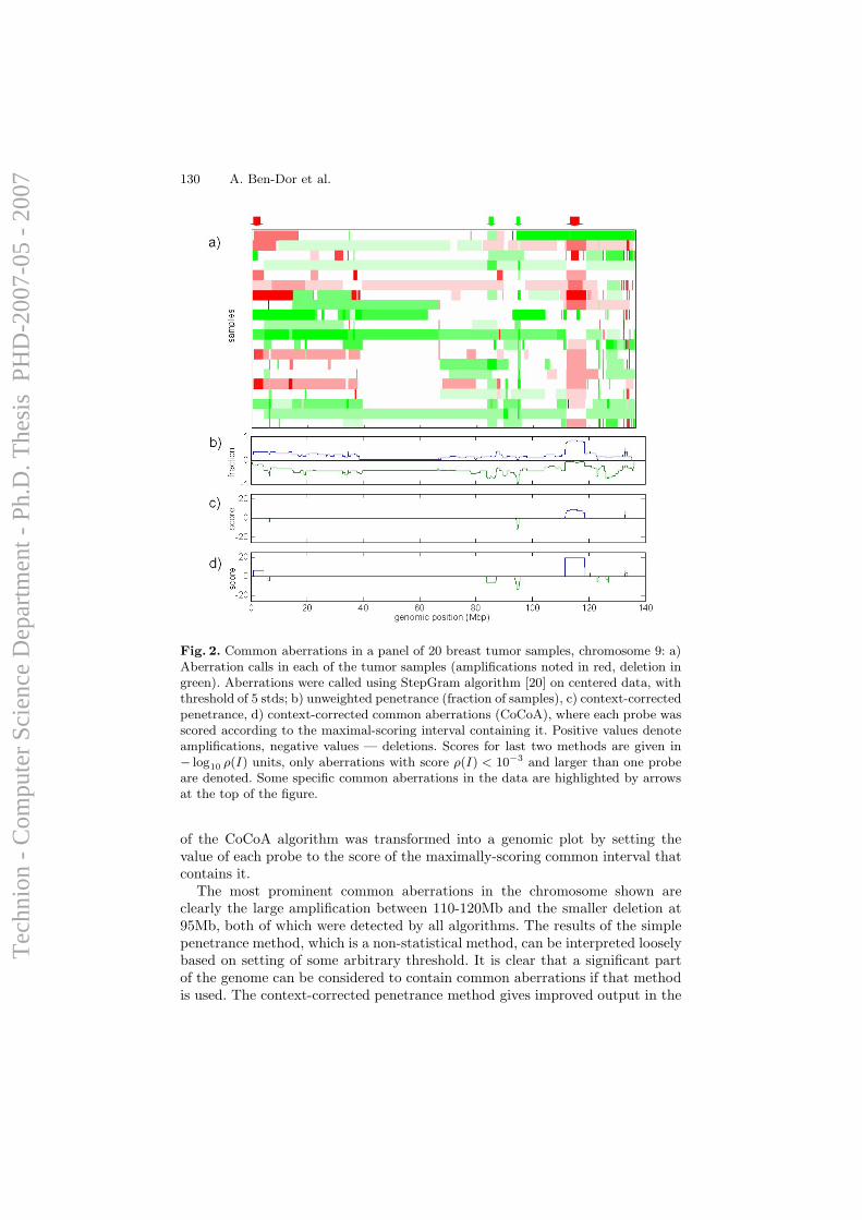
130 A. Ben-Dor et al.
Fig. 2. Common aberrations in a panel of 20 breast tumor samples, chromosome 9: a)Aberration calls in each of the tumor samples (amplifications noted in red, deletion ingreen). Aberrations were called using StepGram algorithm [20] on centered data, withthreshold of 5 stds; b) unweighted penetrance (fraction of samples), c) context-correctedpenetrance, d) context-corrected common aberrations (CoCoA), where each probe wasscored according to the maximal-scoring interval containing it. Positive values denoteamplifications, negative values — deletions. Scores for last two methods are given in− log10 ρ(I) units, only aberrations with score ρ(I) < 10−3 and larger than one probeare denoted. Some specific common aberrations in the data are highlighted by arrowsat the top of the figure.
of the CoCoA algorithm was transformed into a genomic plot by setting thevalue of each probe to the score of the maximally-scoring common interval thatcontains it.
The most prominent common aberrations in the chromosome shown areclearly the large amplification between 110-120Mb and the smaller deletion at95Mb, both of which were detected by all algorithms. The results of the simplepenetrance method, which is a non-statistical method, can be interpreted looselybased on setting of some arbitrary threshold. It is clear that a significant partof the genome can be considered to contain common aberrations if that methodis used. The context-corrected penetrance method gives improved output in the
Tec
hnio
n -
Com
pute
r Sc
ienc
e D
epar
tmen
t - P
h.D
. The
sis
PH
D-2
007-
05 -
200
7
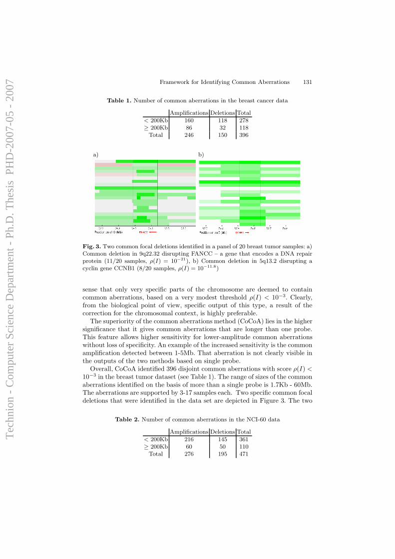
Framework for Identifying Common Aberrations 131
Table 1. Number of common aberrations in the breast cancer data
Amplifications Deletions Total< 200Kb 160 118 278≥ 200Kb 86 32 118
Total 246 150 396
a) b)
Fig. 3. Two common focal deletions identified in a panel of 20 breast tumor samples: a)Common deletion in 9q22.32 disrupting FANCC – a gene that encodes a DNA repairprotein (11/20 samples, ρ(I) = 10−21), b) Common deletion in 5q13.2 disrupting acyclin gene CCNB1 (8/20 samples, ρ(I) = 10−11.8)
sense that only very specific parts of the chromosome are deemed to containcommon aberrations, based on a very modest threshold ρ(I) < 10−3. Clearly,from the biological point of view, specific output of this type, a result of thecorrection for the chromosomal context, is highly preferable.
The superiority of the common aberrations method (CoCoA) lies in the highersignificance that it gives common aberrations that are longer than one probe.This feature allows higher sensitivity for lower-amplitude common aberrationswithout loss of specificity. An example of the increased sensitivity is the commonamplification detected between 1-5Mb. That aberration is not clearly visible inthe outputs of the two methods based on single probe.
Overall, CoCoA identified 396 disjoint common aberrations with score ρ(I) <10−3 in the breast tumor dataset (see Table 1). The range of sizes of the commonaberrations identified on the basis of more than a single probe is 1.7Kb - 60Mb.The aberrations are supported by 3-17 samples each. Two specific common focaldeletions that were identified in the data set are depicted in Figure 3. The two
Table 2. Number of common aberrations in the NCI-60 data
Amplifications Deletions Total< 200Kb 216 145 361≥ 200Kb 60 50 110
Total 276 195 471
Tec
hnio
n -
Com
pute
r Sc
ienc
e D
epar
tmen
t - P
h.D
. The
sis
PH
D-2
007-
05 -
200
7
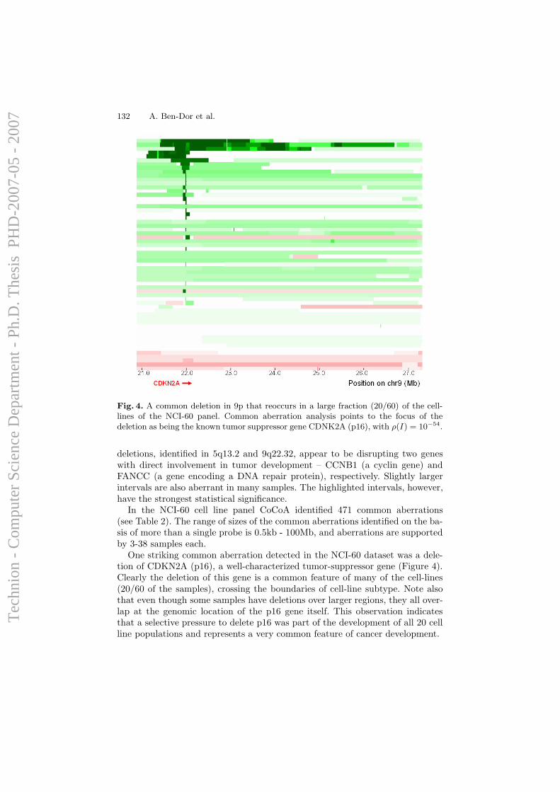
132 A. Ben-Dor et al.
Fig. 4. A common deletion in 9p that reoccurs in a large fraction (20/60) of the cell-lines of the NCI-60 panel. Common aberration analysis points to the focus of thedeletion as being the known tumor suppressor gene CDNK2A (p16), with ρ(I) = 10−54.
deletions, identified in 5q13.2 and 9q22.32, appear to be disrupting two geneswith direct involvement in tumor development – CCNB1 (a cyclin gene) andFANCC (a gene encoding a DNA repair protein), respectively. Slightly largerintervals are also aberrant in many samples. The highlighted intervals, however,have the strongest statistical significance.
In the NCI-60 cell line panel CoCoA identified 471 common aberrations(see Table 2). The range of sizes of the common aberrations identified on the ba-sis of more than a single probe is 0.5kb - 100Mb, and aberrations are supportedby 3-38 samples each.
One striking common aberration detected in the NCI-60 dataset was a dele-tion of CDKN2A (p16), a well-characterized tumor-suppressor gene (Figure 4).Clearly the deletion of this gene is a common feature of many of the cell-lines(20/60 of the samples), crossing the boundaries of cell-line subtype. Note alsothat even though some samples have deletions over larger regions, they all over-lap at the genomic location of the p16 gene itself. This observation indicatesthat a selective pressure to delete p16 was part of the development of all 20 cellline populations and represents a very common feature of cancer development.
Tec
hnio
n -
Com
pute
r Sc
ienc
e D
epar
tmen
t - P
h.D
. The
sis
PH
D-2
007-
05 -
200
7
Framework for Identifying Common Aberrations 133
4 Discussion
In this paper we propose a computational framework for identifying and ana-lyzing copy number aberrations (amplifications and deletions) that occur acrossmultiple samples and for assessing their statistical significance. The frameworkallows using different aberration calling algorithms as input, independent of theirstatistical modeling.
Two central features of our methods are: A)When assessing the significance ofa particular aberration, we use the height of the aberration, as opposed to requir-ing an additional threshold to discretize the aberration calls. B) The ability toaddress the context of the aberration structures in the individual samples. Givena candidate interval, its significance at a particular sample depends not only onthe average height of the candidate interval, but also on the overall prevalenceof aberrations in that sample. We describe two methods that have those impor-tant features. The CoCoA method scores intervals while the context-correctedpenetrance method scores individual loci. In theory, there is a larger statisticalpower in considering multi-loci aberrations as both a supporting sample set anda genomic interval are identified together. Another difference between probe leveland interval level analysis, is that in probe level analysis an additional thresh-olding step is required to determine the boundaries of the common aberrations.Note that for any single locus penetrance based method intervals with consistenthigh scoring can theoretically arise from aberrations in different sets of samples.In practice this is usually not the case. When scoring intervals, as CoCoA does,sample integrity is always preserved: the set of samples over which an interval isreported as a common aberration is the same for all loci spanned by said interval.
Our framework is very efficient. When run on the NCI60 sample set our pro-cess takes under 1 minute, including the first step of single sample aberrationcalling, using StepGram. This enables interactive data analysis that is not pos-sible for less efficient approaches. This combined approach will scale up to largerdatasets and to denser arrays that allow for much finer mapping of aberrant re-gions. We emphasize that this requires not only an efficient approach to commonaberrations but also a very efficient aberration-calling methods.
One important previous formal treatment of calling common aberrations inCGH data is described in [18]. The method described therein, called STAC,is based on a heuristic search seeking to optimize statistical scores assignedto candidate regions of common aberrations. STAC’s search is computationallyintensive and performance is further limited by relying on permutations andsimulations to obtain significance estimates. According to the paper’s Supple-mentary material STAC implementation takes days to run on relatively smalldatasets of 42 and 47 samples, measured using a low resolution (approximately1Mb) technology. STAC treats gains and losses as binary and does not takes intoaccount the exact amplitude of the measured signal.
We have shown examples of applying the framework on a set of breast cancersamples that identify both known and novel cancer related genes. It is interestingto note p16 as a universal deletion in the NCI60 panel. FANCC, a gene from theFanconi anemia group of genes (FA), which codes to a DNA repair protein is
Tec
hnio
n -
Com
pute
r Sc
ienc
e D
epar
tmen
t - P
h.D
. The
sis
PH
D-2
007-
05 -
200
7
134 A. Ben-Dor et al.
deleted in 11 out of the 20 breast cancer samples. FA genes are known to be co-factors interacting with BRCA2 in breast cancer pathogenesis. In a recent study[32] the authors demonstrate a role for the FA pathway in interstrand cross-link repair which is independent from that of BRCA2 in the same process. Thisfinding and our implication of FANCC as a fairly focal common breast cancerdeletion together suggest an important role for FANCC under-functioning incancer pathogenesis.
Lastly, we note that the methods herein presented can be extended to identifydifferential aberrations in DNA copy number data coming from several pheno-typic classes. A more detailed investigation of this application will be the topicof future work.
References
1. Kauraniemi, P., Hautaniemi, S., Autio, R., Astola, J., Monni, O., Elkahloun, A.,Kallioniemi, A.: Effects of Herceptin treatment on global gene expression patternsin HER2-amplified and nonamplified breast cancer cell lines. Oncogene 23(4)(2004) 1010–1013
2. Binh, M., Sastre-Garau, X., Guillou, L., de Pinieux, G., Terrier, P., Lagace, R., Au-rias, A., Hostein, I., Coindre, J.: MDM2 and CDK4 immunostainings are useful ad-juncts in diagnosing well-differentiated and dedifferentiated liposarcoma subtypes:A comparative analysis of 559 soft tissue neoplasms with genetic data. AmericanJournal of Surgical Pathology 29(10) (2005) 1340–1347
3. Balsara, B., Testa, J.: Chromosomal imbalances in human lung cancer. Oncogene21(45) (2002) 6877–83
4. Kallioniemi, O., Kallioniemi, A., Sudar, D., Rutovitz, D., Gray, J., Waldman, F.,Pinkel, D.: Comparative genomic hybridization: a rapid new method for detectingand mapping DNA amplification in tumors. Semin Cancer Biol 4(1) (1993) 41–46
5. Mertens, F., Johansson, B., Hoglund, M., Mitelman, F.: Chromosomal imbalancemaps of malignant solid tumors: a cytogenetic survey of 3185 neoplasms. CancerResearch 57(13) (1997) 2765–80
6. Barrett, M., Scheffer, A., Ben-Dor, A., Sampas, N., Lipson, D., Kincaid, R., Tsang,P., Curry, B., Baird, K., Meltzer, P., Yakhini, Z., Bruhn, L., Laderman, S.: Compar-ative genomic hybridization using oligonucleotide microarrays and total genomicDNA. PNAS 101(51) (2004) 17765–17770
7. Bignell, G., Huang, J., Greshock, J., Watt, S., Butler, A., West, S., Grigorova, M.,Jones, K., Wei, W., Stratton, M., Futreal, P., Weber, B., Shapero, M., Wooster, R.:High-resolution analysis of DNA copy number using oligonucleotide microarrays.Genome Research 14(2) (2004) 287–95
8. Brennan, C., Zhang, Y., Leo, C., Feng, B., Cauwels, C., Aguirre, A., Kim, M.,Protopopov, A., Chin, L.: High-resolution global profiling of genomic alterationswith long oligonucleotide microarray. Cancer Research 64(14) (2004) 4744–8
9. Hedenfalk, I., Ringner, M., Ben-Dor, A., Yakhini, Z., Chen, Y., Chebil, G., Ach,R., Loman, N., Olsson, H., Meltzer, P., Borg, A., Trent, J.: Molecular classificationof familial non-BRCA1/BRCA2 breast cancer. PNAS 100(5) (2003) 2532–7
10. Pinkel, D., Segraves, R., Sudar, D., Clark, S., Poole, I., Kowbel, D., Collins, C.,Kuo, W., Chen, C., Zhai, Y., Dairkee, S., Ljung, B., Gray, J., Albertson, D.: Highresolution analysis of DNA copy number variation using comparative genomic hy-bridization to microarrays. Nature Genetics 20(2) (1998) 207–211
Tec
hnio
n -
Com
pute
r Sc
ienc
e D
epar
tmen
t - P
h.D
. The
sis
PH
D-2
007-
05 -
200
7
Framework for Identifying Common Aberrations 135
11. Pollack, J., Perou, C., Alizadeh, A., Eisen, M., Pergamenschikov, A., Williams, C.,Jeffrey, S., Botstein, D., Brown, P.: Genome-wide analysis of DNA copy-numberchanges using cDNA microarrays. Nature Genetics 23(1) (1999) 41–6
12. Sebat, J., Lakshmi, B., Troge, J., Alexander, J., Young, J., Lundin, P., Maner, S.,Massa, H., Walker, M., Chi, M., Navin, N., Lucito, R., Healy, J., Hicks, J., Ye,K., Reiner, A., Gilliam, T., Trask, B., Patterson, N., Zetterberg, A., Wigler, M.:Large-scale copy number polymorphism in the human genome. Science 305(5683)(2004) 525–8
13. Fridlyand, J., Snijders, A., Pinkel, D., Albertson, D., Jain, A.: Hidden markovmodels approach to the analysis of array cgh data. Journal of Multivariate Analysis90 (2004) 132–153
14. Lai, W., Johnson, M., Kucherlapati, R., Park, P.: Comparative analysis of algo-rithms for identifying amplifications and deletions in array CGH data. Bioinfor-matics 21(19) (2005) 3763–70
15. Olshen, A., Venkatraman, E., Lucito, R., Wigler, M.: Circular binary segmentationfor the analysis of array-based dna copy number data. Biostatistics 5 (2004) 557–72
16. Wang, P., Kim, Y., Pollack, J., Narasimhan, B., Tibshirani, R.: A method forcalling gains and losses in array CGH data. Biostatistics 6 (2005) 45–58
17. Willenbrock, H., Fridlyand, J.: A comparison study: applying segmentation toarray CGH data for downstream analyses. Bioinformatics 21(22) (2005) 4084–91
18. Diskin, S., Eck, T., Greshock, J., Mosse, Y., Naylor, T., Stoeckert, C., Weber, B.,Maris, J., Grant, G.: STAC: a method for testing the significance of DNA copynumber aberrations across multiple array-CGH experiments. Genome Research 16(2006) 1149–1158
19. Rouveirol, C., Stransky, N., Hupe, P., Rosa, P.L., Viara, E., Barillot, E., Radvanyi,F.: Computation of reccurant minimla genomic alterations from array-cgh data.Bioinformatics (2006) 849–856
20. Lipson, D., Aumann, Y., Ben-Dor, A., Linial, N., Yakhini, Z.: Efficient calculationof interval scores for DNA copy number data analysis. Journal of ComputationalBiology 13(2) (2006) 215–28
21. Lingjarde, O.C., Baumbusch, L.O., Liestol, K., Glad, I.K., Borresen-Dale, A.L.:Cgh-explorer: a program for analysis of array-cgh data. Bioinformatics 21(6)(2005) 821–822
22. Wiedswang, G., Borgen, E., Kvalheim, R.K.G., Nesland, J., Qvist, H., Schlichting,E., Sauer, T., Janbu, J., Harbitz, T., Naume, B.: Detection of isolated tumor cellsin bone marrow is an independent prognostic factor in breast cancer. Journal ofClinical Oncology 21 (2003) 3469–3478
23. Sorlie, T., Perou, C., Tibshirani, R., Aas, T., Geisler, S., Johnsen, H., Hastie, T.,Eisen, M., van de Rijn, M., Jeffrey, S., Thorsen, T., Quist, H., Matese, J., Brown,P., Botstein, D., Lonning, P.E., Borresen-Dale, A.: Gene expression patterns ofbreast carcinomas distinguish tumor subclasses with clinical implications. PNAS98(10) (2001) 10869–74
24. Sorlie, T., Wang, Y., Xiao, C., Johnsen, H., Naume, B., Samaha, R., Borresen-Dale, A.L.: Distinct molecular mechanisms underlying clinically relevant subtypesof breast cancer: Gene expression analyses across three different platforms. BMCGenomics 7 (2006) 127
25. Weinstein, J., Myers, T., O’Connor, P., Friend, S., Jr., A.F., Kohn, K., Fojo, T.,Bates, S., Rubinstein, L., Anderson, N., Buolamwini, J., van Osdol, W., Monks, A.,Scudiero, D., Sausville, E., Zaharevitz, D., Bunow, B., Viswanadhan, V., Johnson,G., Wittes, R., Paull, K.: An information-intensive approach to the molecularpharmacology of cancer. Science 275(10) (1997) 343–49
Tec
hnio
n -
Com
pute
r Sc
ienc
e D
epar
tmen
t - P
h.D
. The
sis
PH
D-2
007-
05 -
200
7
136 A. Ben-Dor et al.
26. Monks, A., Scudiero, D., Skehan, P., Shoemaker, R., Paull, K., Vistica, D., Hose,C., Langley, J., Cronise, P., et al., A.V.W.: Feasibility of a high-flux anticancerdrug screen using a diverse panel of cultured human tumor cell lines. Journal ofthe National Cancer Institute 83 (1991) 757–66
27. Shoemaker, R., Monks, A., Alley, M., Scudiero, D., Fine, D., McLemore, T.,Abbott, B., Paull, K., Mayo, J., Boyd, M.: Development of human tumor cellline panels for use in disease-oriented drug screening. Progress in Clinical andBiological Research 276 (1988) 265–86
28. Nishizuka, S., Charboneau, L., Young, L., Major, S., Reinhold, W., Waltham, M.,Kouros-Mehr, H., Bussey, K., Lee, J., Espina, V., Munson, P., 3rd, E.P., Liotta,L., Weinstein, J.: Proteomic profiling of the nci-60 cancer cell lines using newhigh-density reverse-phase lysate microarrays. PNAS 100 (2003) 14229–34
29. Paull, K., Shoemaker, R., Hodes, L., Monks, A., Scudiero, D., Rubinstein, L.,Plowman, J., Boyd, M.: Display and analysis of patterns of differential activity ofdrugs against human tumor cell lines: development of mean graph and comparealgorithm. Journal of the National Cancer Institute 81 (1989) 1088–92
30. Shi,L.,Fan,Y.,Lee, J.,Waltham,M.,Andrews,D.T., Scherf,U.,Paull,K.,Weinstein,J.: Mining and visualizing large anticancer drug discovery databases. Journal ofChemical Information and Computer Sciences 40 (2000) 367–79
31. Staunton, J., Slonim, D., Coller, H., Tamayo, P., Angelo, M., Park, J., Scherf, U.,Lee, J., Reinhold, W., Weinstein, J., Mesirov, J., Lander, E., Golub, T.: Chemosen-sitivity prediction by transcriptional profiling. PNAS 98 (2001) 10787–92
32. Kitao, H., Yamamoto, K., Matsushita, N., Ohzeki, M., Ishiai, M., Takata, M.:Functional interplay between brca2/fancd1 and fancc in dna repair. Journal ofBiological Chemistry 281(30) (2006) 21312–21320
Tec
hnio
n -
Com
pute
r Sc
ienc
e D
epar
tmen
t - P
h.D
. The
sis
PH
D-2
007-
05 -
200
7

Tec
hnio
n -
Com
pute
r Sc
ienc
e D
epar
tmen
t - P
h.D
. The
sis
PH
D-2
007-
05 -
200
7
A.6 Joint Analysis of DNA Copy Numbers
and Gene Expression Levels
Doron Lipson, Amir Ben-Dor, Elinor Dehan, and Zohar Yakhini. “JointAnalysis of DNA Copy Numbers and Gene Expression Levels”.Proceedings of WABI 2004, LNCS 3240, p. 135, Springer-Verlag, 2004.
125
Tec
hnio
n -
Com
pute
r Sc
ienc
e D
epar
tmen
t - P
h.D
. The
sis
PH
D-2
007-
05 -
200
7

126
Tec
hnio
n -
Com
pute
r Sc
ienc
e D
epar
tmen
t - P
h.D
. The
sis
PH
D-2
007-
05 -
200
7
Joint Analysis of DNA Copy Numbersand Gene Expression Levels
Doron Lipson1, Amir Ben-Dor2, Elinor Dehan3, and Zohar Yakhini2
1 Computer Science Dept., Technion, [email protected], corresponding author
2 Agilent Laboratories, Palo Alto, CA{amir ben-dor, zohar yakhini}@agilent.com
3 Functional Genomics Unit, Sheba Medical Center, [email protected]
Abstract. Genomic instabilities, amplifications, deletions and translo-cations are often observed in tumor cells. In the process of cancer patho-genesis cells acquire multiple genomic alterations, some of which drive theprocess by triggering overexpression of oncogenes and by silencing tumorsuppressors and DNA repair genes. We present data analysis methodsdesigned to study the overall transcriptional effects of DNA copy num-ber alterations. Alterations can be measured using several techniquesincluding microarray based hybridization assays. The data have uniqueproperties due to the strong dependence between measurement valuesin close genomic loci. To account for this dependence in studying thecorrelation of DNA copy number to expression levels we develop ver-sions of standard correlation methods that apply to genomic regions andmethods for assessing the statistical significance of the observed results.In joint DNA copy number and expression data we define significantlyaltered submatrices as submatrices where a statistically significant cor-relation of DNA copy number to expression is observed. We developheuristic approaches to identify these structures in data matrices. Weapply all methods to several datasets, highlighting results that can notbe obtained by direct approaches or without using the regional view.
1 Introduction
Alterations in DNA copy number (DCN ) are characteristic of many cancertypes and are thought to drive some cancer pathogenesis processes. Alterationsinclude large chromosomal gains and losses as well as smaller scale amplifi-cations and deletions. Genomic instability triggers the overexpression or acti-vation of oncogenes and the silencing of tumor suppressors and DNA repairgenes. Alterations in DCN have been initially measured using local fluorescencein situ hybridization-based techniques. These evolved to a genome wide tech-nique called Comparative Genomic Hybridization (CGH, see [8]), now commonlyused for the identification of chromosomal alterations in cancer [10, 2]). In thisgenome-wide cytogenetic method differentially labelled tumor and normal DNA
Tec
hnio
n -
Com
pute
r Sc
ienc
e D
epar
tmen
t - P
h.D
. The
sis
PH
D-2
007-
05 -
200
7
2 Doron Lipson et al
are co-hybridized to normal metaphases. Fluorescence level ratios between thetwo labels allow the detection of chromosomal amplifications and deletions. Thismethod has, however, a limited resolution (10-20 Mbp) which maks it impossibleto predict the borders of chromosomal changes or to identify changes in copynumbers of single genes and small genomic regions. In a more advanced methodtermed array CGH (aCGH) the tumor and normal DNA are co-hybridized toa microarray of thousands of genomic clones of BAC, cDNA or oligonucleotideprobes ([13, 11, 6]). The use of aCGH allows the determination of changes in DCNof relatively small chromosomal regions. When using oligonucleotide arrays theresolution can, in theory, be finer than single genes.
The development of high resolution mapping of DCN alterations and theprogress of expression profiling technologies enable the study of the effects ofchromosomal alterations on cellular processes and how these are mediated throughaltered expression of genes residing in altered regions. By measuring DNA copynumbers and mRNA expression levels on the same set of samples we gain accessto the relationship of copy number alterations to how they are manifested inaltering expression profiles. In [12] the authors used (metaphase slides) CGHto identify large scale amplifications in 23 metastatic colon cancer samples andperformed expression profiling on the same samples. They observed some cor-relation between DCN and expression levels but on overall effect of alterationson transciption. In [14] an opposite observation is reported, for breast cancersamples. That is: a strong global correlation between copy number changes andexpression level variation is observed. Similarly, Hyman et al [7] studied copynumber alterations in 14 breast cancer cell lines and identified 270 genes withexpression levels that are systematically attributable to gene amplification. Thestatistics used by both latter studies is based on simulations and takes into ac-count single gene correlations but not local regional effects. Recently, Linn etal studied expression patterns and genome alterations in DFSP and discoveredcommon 17q and 22q amplifications that are associated with elevated expressionof resident genes [9].
Our purpose in this paper is to provide algorithmic and statistical methods torigorously support data analysis designed to improve our understanding of copynumber to transcription relationships (specifically in aCGH data). Regions ofhigh correlation are potentially related to the tumor pathogenesis. More specifi-cally, genes affected by changes in DCN potentially play a role in driving tumordifferentiation. Note that the correlation between expression data vectors andtheir corresponding (same gene) DCN data vectors should behave completelyrandom if all the variation in the DCN vector arises due to experimental errors.We are therefore mostly interested in detection of statistically significant corre-lations. These might not show up when low resolution and global data analysisapproaches are employed. For example, low penetrance (not all cells in the sam-ple) and low prevalence (not all samples in the study) alterations might effectexpression below the 2-fold mark and only in some of the samples, but in a sig-nificant manner when a genomic region is considered. In addition – the detectionof regions that manifest a significant correlation can aid in detecting actual low
Tec
hnio
n -
Com
pute
r Sc
ienc
e D
epar
tmen
t - P
h.D
. The
sis
PH
D-2
007-
05 -
200
7
Joint Analysis of DNA Copy Numbers and Gene Expression Levels 3
penetrance alterations in high resolution even if the DCN data, alone, do notsupport such discoveries.
Throughout the paper we use C and E to denote the DNA copy number andgene expression data matrices, where the (i, j)-th entry of each matrix representthe data for the ith gene in the jth sample. We abbreviate “DNA copy number”and “gene expression” as DCN and GE respectively.
In Section 2 we describe methods to quantify the correlation observed forany pair of rows C(i, ·) and E(i, ·). In Section 3 we extend these to account forthe regional character of DCN alterations. In Section 4 we discuss submatricesof affected samples and genes. Conclusions are discussed in Section 5.
Datasets We demonstrate our methods on two joint DCN-GE breast cancerdatasets. The first, described in [14] is of 6,095 genes across 41 samples (4 celllines, 37 primary breast tumors). The second, from [7] is of 13,824 genes across14 cell-line samples. All datasets are measured on cDNA microarrays.
2 Correlation Scoring Methods
Consider a single gene g and let u = ug and v = vg denote the correspondingDCN and GE data vectors of g. Let n denote the number of samples (length ofu and v). In this section we present several approaches for scoring g by lookingfor dependencies between u and v.
2.1 Pearson Product Moment Correlation
The most common measure of the dependence between two vectors u, v is thePearson correlation coefficient:
r(u, v) =∑
(u− u)(v − v)√∑(u− u)2
√∑(v − v)2
. (1)
r measures the degree to which u and v maintain a linear relationship. It maytherefore be less suitable when the DCN and GE values follow some non-linearrelationship. Nonetheless, previous large-scale DCN-GE comparative studies [14]used Pearson correlation as a sole scoring method to evaluate dependence.
2.2 Separating-Cross Correlation
A different methodology for comparing gene copy measurements with gene ex-pression levels, such as the one described in [7] utilizes user chosen thresholdsfor classifying DCN measurements as deleted or amplified and for classifying GEmeasurements as under-expressed or over-expressed. Such methods do not relyon any assumption of linearity or on the value of the mean; however, they aresomewhat dependent on the specific choice of thresholds. The separating-crossesscores we now introduce are a generalized approach to threshold-based analysisof the dependence between two vectors.
Tec
hnio
n -
Com
pute
r Sc
ienc
e D
epar
tmen
t - P
h.D
. The
sis
PH
D-2
007-
05 -
200
7
4 Doron Lipson et al
We can view the two vectors u and v as n points (ui, vi) in the plain. An axisparallel cross t = tx,y, centered at (x, y), partitions the plain into four quadrants,denoted by At, Bt, Ct, and Dt (See figure 2). We denote by at the number ofpoints (ui, vi) that belong to the quadrant At. The other quadrants counts bt, ct
and dt are defined similarly. Clearly, at + bt + ct + dt = n.Roughly speaking, u and v are correlated if there exist a cross t such that both
a and d are large (compared with b and c). More generally, assume we are givena function of the quadrants counts (such a function is called a cross-function),f(a, b, c, d). We are interested in the maximal obtainable value of f :
F (u, v) = maxt{f(at, bt, ct, dt)}. (2)
The function F is called a separating cross score function.Let π denote the ranks of the samples with respect to the vector u. That is,
u(π−1(1)) < · · · < u(π−1(n)). For example, for u = (2, 1.5, 9, 0.4), π = (3, 2, 4, 1).Similarly, we denote by τ the samples permutation induced by v. Since cross-functions (and thus score functions) depend only on quadrants counts and noton the actual locations of the points, we have F (u, v) = F (π, τ). Thus, forevery function f(π, τ, t), we can compute F (π, τ) by examining (n−1)2 possiblecrosses. We describe one cross score function, the Maximal Diagonal Product(MDP). Consider the separating-cross-function DP(π, τ, t) = at · dt, which wecall Diagonal Product (DP), and the corresponding score function:
MDP(π, τ) = maxt{DP(π, τ, t)}. (3)
A useful attribute of the MDP score is that it provides a distinction betweensamples that contribute to the maximum score (points within At and Dt) andthose that do not (points within Bt and Ct). We make use of this attribute inidentifying affected samples in Section 4. The combinatorial nature of this scoreallows rigorous calculation of its statistical properties, the discussion of which isbeyond the scope of this paper.
3 Regional Analysis
Some cancer related alterations in genomic DNA have direct effect on mRNAlevels, possibly leading to downstream functional deficiencies. These alterationsare most likely localized in one or more of the following aspects:
1. The alteration in genomic DNA is limited to certain chromosomal segments.2. The expression of all genes within a specific genomic segment may not be
effected to the same extent.3. Not all samples contain identical or similar genomic alterations.4. Within specific samples, alterations occur with varying levels of penetrance.
Previous work on DCN-GE expression relationship consider only correlationbetween the gene-expression levels of single genes and their respective DNA copy
Tec
hnio
n -
Com
pute
r Sc
ienc
e D
epar
tmen
t - P
h.D
. The
sis
PH
D-2
007-
05 -
200
7
Joint Analysis of DNA Copy Numbers and Gene Expression Levels 5
number measurements. Pollack et al [14] study the global behavior of DCN-GEcorrelation and show that the distribution of Pearson correlation values betweenDCN and GE differs from the expected distribution. They report 54 amplifiedgenes with moderately or highly elevated expression levels. Hyman et al [7]also demonstrate global single gene correlations and identify 270 genes withexpression levels significantly influenced by changes in DCN .
CGH based studies show that chromosomal alterations frequently apply tolong stretches of the genome that may span a large number of genes. The ex-pression pattern of a gene that is affected by such an aberration is expected tocorrelate not only with the copy number of its own coding DNA but also withthe DCN measurements of neighboring genes. We therefore expect that analysisthat takes regional effects into account to yield better results that might offsetthe negative effects of noise in the data or low penetrance. Both [14] and [7] didnot account for such regional considerations. In this section we suggest a frame-work for considering local correlation between genomic alteration and variancein gene expression levels, that accounts for regional effects.
Given a gene gi we define its k-neighborhood as the continuous sequenceof genes indexed by Γk(i) = (i − k, ..., i + k). A straightforward approach toquantifying the correlation of the gene’s GE vector E(i, ·) with the DCN vectorsin its neighborhood Γk(i) is by calculating the average correlation of E(i, ·) toeach of the respective DCN vectors:
r(i, Γk(i)) =1
2k + 1
i+k∑j=i−k
r(i, j), (4)
where r(i, j) is any correlation measure between the vectors E(i, ·) and C(j, ·).Alternative approaches to regional correlation include the correlation of E(i, ·)
to the vector of (weighted or uniform) average DCN in Γk(i), or the product ofthe p-values of the respective correlations.
Permuted Data When performing analyses that take gene order into account wecompare results to a null model that assumes neighboring genes are indepen-dent of each other. To this end, we also perform our analysis on gene-permutedmatrices E′ and C ′ where the same permutation was applied to the rows ofboth matrices. We expect regional effect results to be dependent on the originalchromosomal order of the genes.
Computing p-Values To identify regions where DCN and GE correlate beyondthe extent expected for the consistent DCN values we perform the simulationanalysis outlined below. The general idea is to evaluate a locus dependent p-value for chromosomal regions. Correlations in regions where a very consistentDCN measurements are observed need to cross much higher thresholds to besignificant since distributions expected at random in such regions have largervariation (weaker smoothing effect of averaging because of the consistent DCNvalues). Consider a neighborhood Γk(i) and fix L, the size of simulation applied.We randomly draw L−1 expression vectors (rows of E) indexed by i1, i2, ..., iL−1,
Tec
hnio
n -
Com
pute
r Sc
ienc
e D
epar
tmen
t - P
h.D
. The
sis
PH
D-2
007-
05 -
200
7
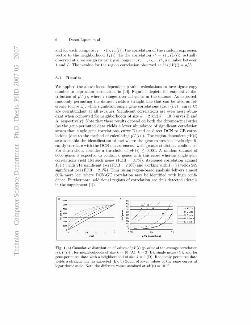
6 Doron Lipson et al
and for each compute rl = r(il, Γk(i)), the correlation of the random expressionvector to the neighborhood Γk(i). To the correlation r∗ = r(i, Γk(i)), actuallyobserved at i, we assign its rank ρ amongst r1, r2, ..., rL−1, r
∗, a number between1 and L. The p-value for the region correlation observed at i is pV (i) = ρ/L.
3.1 Results
We applied the above locus dependent p-value calculations to investigate copynumber to expression correlations in [14]. Figure 1 depicts the cumulative dis-tribution of pV (i), where i ranges over all genes in the dataset. As expected,randomly permuting the dataset yields a straight line that can be used as ref-erence (curve E), while significant single gene correlations (i.e. r(i, i) , curve C)are overabundant at all p-values. Significant correlations are even more abun-dant when computed for neighborhoods of size k = 2 and k = 10 (curves B andA, respectively). Note that these results depend on both the chromosomal order(as the gene-permuted data yields a lower abundance of significant correlationscores than single gene correlations, curve D) and on direct DCN to GE corre-lations (due to the method of calculating pV (i) ). The region-dependent pV (i)scores enable the identification of loci where the gene expression levels signifi-cantly correlate with the DCN measurements with greater statistical confidence.For illustration, consider a threshold of pV (i) ≤ 0.001. A random dataset of6000 genes is expected to contain 6 genes with this score whereas single genecorrelations yield 164 such genes (FDR = 3.7%). Averaged correlation againstΓ2(i) yields 214 significant loci (FDR = 2.8%) and working with Γ10(i) yields 289significant loci (FDR = 2.1%). Thus, using region-based analysis delivers almost80% more loci where DCN-GE correlation may be identified with high confi-dence. Furthermore, additional regions of correlation are thus detected (detailsin the supplement [1]).
Fig. 1. a) Cumulative distribution of values of pV (i) (p-value of the average correlationr(i, Γ (i))), for neighborhoods of size k = 10 (A), k = 2 (B), single genes (C), and forgene-permuted data with a neighborhood of size k = 2 (D). Randomly permuted datayields a straight line, as expected (E). b) Zoom of lower values of the same curves atlogarithmic scale. Note the different values attained at pV (i) = 10−3.
Tec
hnio
n -
Com
pute
r Sc
ienc
e D
epar
tmen
t - P
h.D
. The
sis
PH
D-2
007-
05 -
200
7
Joint Analysis of DNA Copy Numbers and Gene Expression Levels 7
4 Genomic-Continuous Submatrices
In the previous section we mentioned that genomic alterations are often localizedto a subset of the samples as well as to a specific chromosomal segment. In thissection we discuss the task of detecting both the genomic segment in which anaberration has occurred, the affected samples and the transcriptional effect ofthe aberration. To this end we define a model of significantly altered genomic-continuous submatrices and present two algorithmic approaches for detectingthem. We then apply the suggested methods to the two breast cancer datasets.
4.1 Definition
For a given pair of DCN and GE matrices C,E over an ordered set of genes Gand a set of samples S we define a genomic-continuous submatrix (GCSM) asM = G′ × S′ where G′ ⊂ G is a continuous segment of genes and S′ ⊆ S is asubset of samples, and its complement submatrix M = G′×{S−S′}. Let C(M)and E(M) denote the projections of the matrices C and E on the subsets G′
and S′ (the DCN and GE submatrices corresponding to M).Under our biological model, a genomic alteration in a given chromosomal
segment and a given sample should affect most of the DCN measurements inthis segment but only some of the respective GE measurements (since changesin expression depend on other factors that determine regulation). Informally, wesay that a given GCSM M is significantly amplified if:
– Most DNA copy values in the set C(M) are positive.– Some genes gi ∈ G′ have higher expression values {E(i, j) : sj ∈ S′} com-
pared to {E(i, j) : sj /∈ S′}.
More formally, let us define a score that reflects the degree to which M issignificantly amplified. First, we define a score F (M ;C) that reflects overabun-dance of positive values in C(M) in comparison to C(M) using the hypergeo-metric distribution. Let N = |C(M ∪M)| and n = |C(M)|. Let K and k be thenumber of positive values in C(M ∪M) and C(M), respectively. Given N,n,Kthe hypergeometric probability of finding k or more positive values in C(M) is:
F (M ;C) = HG(N,K, n, k) =N∑
i=k
(ni
)(N−nK−i
)(NK
) . (5)
Similarly, we define a score F (M ;E) that reflects the overabundance of genesin G′ that are significantly differentially expressed, comparing S′ and S − S′,in the correct direction (higher in S′ than in S − S′). A TNoM (ThresholdNumber of Misclassifications) score may be assigned to each gene according toits performance as a S′ versus S − S′ classifier [5, 3]. Rigorous p-values can becalculated for TNoM. If the probability, for a single gene, of obtaining a scoreof s or better under the null model is p(s) then the number of genes with scoress or better, amongst the |G′| genes examined, is Binomial(n, p(s)) distributed.
Tec
hnio
n -
Com
pute
r Sc
ienc
e D
epar
tmen
t - P
h.D
. The
sis
PH
D-2
007-
05 -
200
7
8 Doron Lipson et al
Let n(s) denote the number of genes with such scores actually observed in thedata. Let σ(s) be the tail probability of the Binomial(n, p(s)) distribution, atn(s). F (M ;E) is then defined to be max0≤s≤|S′|− log(σ(s)). For a more detaileddescription of differential expression overabundance please see [4].
Under the null model, DCN and GE vectors are completely uncorrelated. Atotal score for an amplification in M is:
F (M ;C,E) = − [log10 F (M ;C) + log10 F (M ;E)] (6)
The above discussion addresses amplifications only. However, any deletion ina subset S′ is equivalent, under F , to an amplification in S − S′.
4.2 Algorithmic Approach
Locating a partition of samples that maximizes TNoM overabundance for a givenset of genes is by itself a difficult task that has been approached by heuristicmethods [4]. The problem of locating a partition that maximizes a combinedhypergeometric and TNoM overabundance score is clearly at least as hard, andconsequently we resort to heuristic approaches for locating significantly alteredGCSMs. Note that due to the fact that we are looking for continuous segmentsonly, all possible segments may be enumerated in O(n2), where n is the number ofgenes. The difficulty remains in determining which subset S′ maximizes F ((G′×S′);C,E) for a given segment G′. We suggest two algorithmic approaches:
Max-Hypergeometric Algorithm As the definition of the score of a GCSMM is composed of two parts, a reasonable heuristic approach to locating high-scoring GCSMs is to select the sample partitions that maximize one part ofthe score – the hypergeometric score – for each possible segment, and for thesepartitions to calculate the combined score. For a given segment G′ the calculationof maxS′⊆S [− log(F ((G′×S′);C)] may be performed in (O(|S|)) time by orderingthe samples according to decreasing number of positive entries, as described inthe following psuedo code:
Algorithm 1 MHA - Max-Hypergeometric AlgorithmInput: C, E, t - a significance threshold, l - maximum segment length.Output: A list of high scoring GCSMs, L.for all segments G′ ⊂ G of length ≤ l do
For each sample si ∈ S let pi =# of positive entries in C(G′, si).Order the samples s.t. pπ(1) ≥ ... ≥ pπ(|S|).maxScore = max1≤i<|S| F ((G′, {Sπ(1), ..., Sπ(i)}); C, E).if maxScore > t then
Add M = (G′, S′) to L.
Consistent Correlation Algorithm One shortcoming of MHA is that it de-pends on a sufficiently strong pattern in the DCN measurements alone in order
Tec
hnio
n -
Com
pute
r Sc
ienc
e D
epar
tmen
t - P
h.D
. The
sis
PH
D-2
007-
05 -
200
7
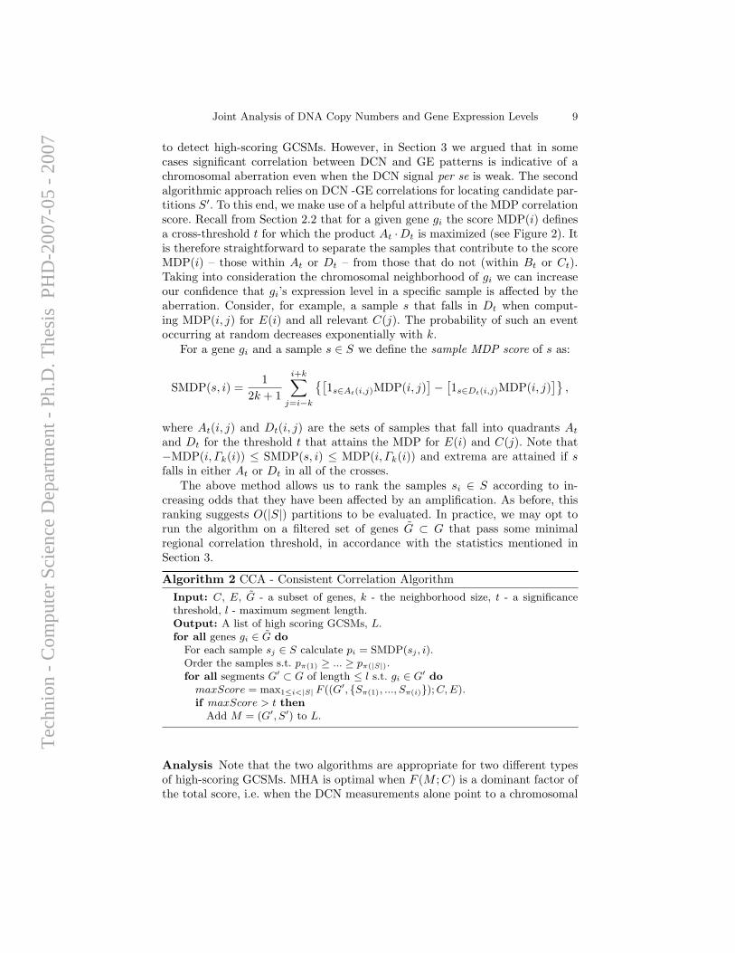
Joint Analysis of DNA Copy Numbers and Gene Expression Levels 9
to detect high-scoring GCSMs. However, in Section 3 we argued that in somecases significant correlation between DCN and GE patterns is indicative of achromosomal aberration even when the DCN signal per se is weak. The secondalgorithmic approach relies on DCN -GE correlations for locating candidate par-titions S′. To this end, we make use of a helpful attribute of the MDP correlationscore. Recall from Section 2.2 that for a given gene gi the score MDP(i) definesa cross-threshold t for which the product At ·Dt is maximized (see Figure 2). Itis therefore straightforward to separate the samples that contribute to the scoreMDP(i) – those within At or Dt – from those that do not (within Bt or Ct).Taking into consideration the chromosomal neighborhood of gi we can increaseour confidence that gi’s expression level in a specific sample is affected by theaberration. Consider, for example, a sample s that falls in Dt when comput-ing MDP(i, j) for E(i) and all relevant C(j). The probability of such an eventoccurring at random decreases exponentially with k.
For a gene gi and a sample s ∈ S we define the sample MDP score of s as:
SMDP(s, i) =1
2k + 1
i+k∑j=i−k
{[1s∈At(i,j)MDP(i, j)
]−
[1s∈Dt(i,j)MDP(i, j)
]},
where At(i, j) and Dt(i, j) are the sets of samples that fall into quadrants At
and Dt for the threshold t that attains the MDP for E(i) and C(j). Note that−MDP(i, Γk(i)) ≤ SMDP(s, i) ≤ MDP(i, Γk(i)) and extrema are attained if sfalls in either At or Dt in all of the crosses.
The above method allows us to rank the samples si ∈ S according to in-creasing odds that they have been affected by an amplification. As before, thisranking suggests O(|S|) partitions to be evaluated. In practice, we may opt torun the algorithm on a filtered set of genes G ⊂ G that pass some minimalregional correlation threshold, in accordance with the statistics mentioned inSection 3.
Algorithm 2 CCA - Consistent Correlation AlgorithmInput: C, E, G - a subset of genes, k - the neighborhood size, t - a significancethreshold, l - maximum segment length.Output: A list of high scoring GCSMs, L.for all genes gi ∈ G do
For each sample sj ∈ S calculate pi = SMDP(sj , i).Order the samples s.t. pπ(1) ≥ ... ≥ pπ(|S|).for all segments G′ ⊂ G of length ≤ l s.t. gi ∈ G′ do
maxScore = max1≤i<|S| F ((G′, {Sπ(1), ..., Sπ(i)}); C, E).if maxScore > t then
Add M = (G′, S′) to L.
Analysis Note that the two algorithms are appropriate for two different typesof high-scoring GCSMs. MHA is optimal when F (M ;C) is a dominant factor ofthe total score, i.e. when the DCN measurements alone point to a chromosomal
Tec
hnio
n -
Com
pute
r Sc
ienc
e D
epar
tmen
t - P
h.D
. The
sis
PH
D-2
007-
05 -
200
7
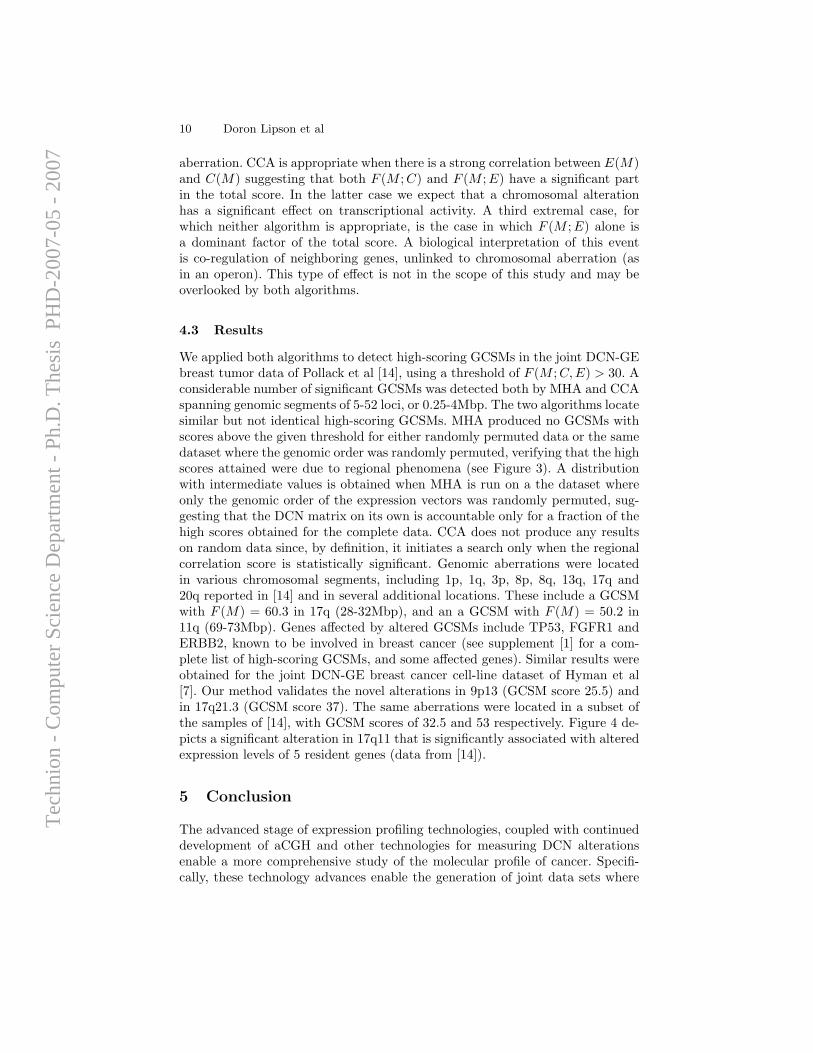
10 Doron Lipson et al
aberration. CCA is appropriate when there is a strong correlation between E(M)and C(M) suggesting that both F (M ;C) and F (M ;E) have a significant partin the total score. In the latter case we expect that a chromosomal alterationhas a significant effect on transcriptional activity. A third extremal case, forwhich neither algorithm is appropriate, is the case in which F (M ;E) alone isa dominant factor of the total score. A biological interpretation of this eventis co-regulation of neighboring genes, unlinked to chromosomal aberration (asin an operon). This type of effect is not in the scope of this study and may beoverlooked by both algorithms.
4.3 Results
We applied both algorithms to detect high-scoring GCSMs in the joint DCN-GEbreast tumor data of Pollack et al [14], using a threshold of F (M ;C,E) > 30. Aconsiderable number of significant GCSMs was detected both by MHA and CCAspanning genomic segments of 5-52 loci, or 0.25-4Mbp. The two algorithms locatesimilar but not identical high-scoring GCSMs. MHA produced no GCSMs withscores above the given threshold for either randomly permuted data or the samedataset where the genomic order was randomly permuted, verifying that the highscores attained were due to regional phenomena (see Figure 3). A distributionwith intermediate values is obtained when MHA is run on a the dataset whereonly the genomic order of the expression vectors was randomly permuted, sug-gesting that the DCN matrix on its own is accountable only for a fraction of thehigh scores obtained for the complete data. CCA does not produce any resultson random data since, by definition, it initiates a search only when the regionalcorrelation score is statistically significant. Genomic aberrations were locatedin various chromosomal segments, including 1p, 1q, 3p, 8p, 8q, 13q, 17q and20q reported in [14] and in several additional locations. These include a GCSMwith F (M) = 60.3 in 17q (28-32Mbp), and an a GCSM with F (M) = 50.2 in11q (69-73Mbp). Genes affected by altered GCSMs include TP53, FGFR1 andERBB2, known to be involved in breast cancer (see supplement [1] for a com-plete list of high-scoring GCSMs, and some affected genes). Similar results wereobtained for the joint DCN-GE breast cancer cell-line dataset of Hyman et al[7]. Our method validates the novel alterations in 9p13 (GCSM score 25.5) andin 17q21.3 (GCSM score 37). The same aberrations were located in a subset ofthe samples of [14], with GCSM scores of 32.5 and 53 respectively. Figure 4 de-picts a significant alteration in 17q11 that is significantly associated with alteredexpression levels of 5 resident genes (data from [14]).
5 Conclusion
The advanced stage of expression profiling technologies, coupled with continueddevelopment of aCGH and other technologies for measuring DCN alterationsenable a more comprehensive study of the molecular profile of cancer. Specifi-cally, these technology advances enable the generation of joint data sets where
Tec
hnio
n -
Com
pute
r Sc
ienc
e D
epar
tmen
t - P
h.D
. The
sis
PH
D-2
007-
05 -
200
7
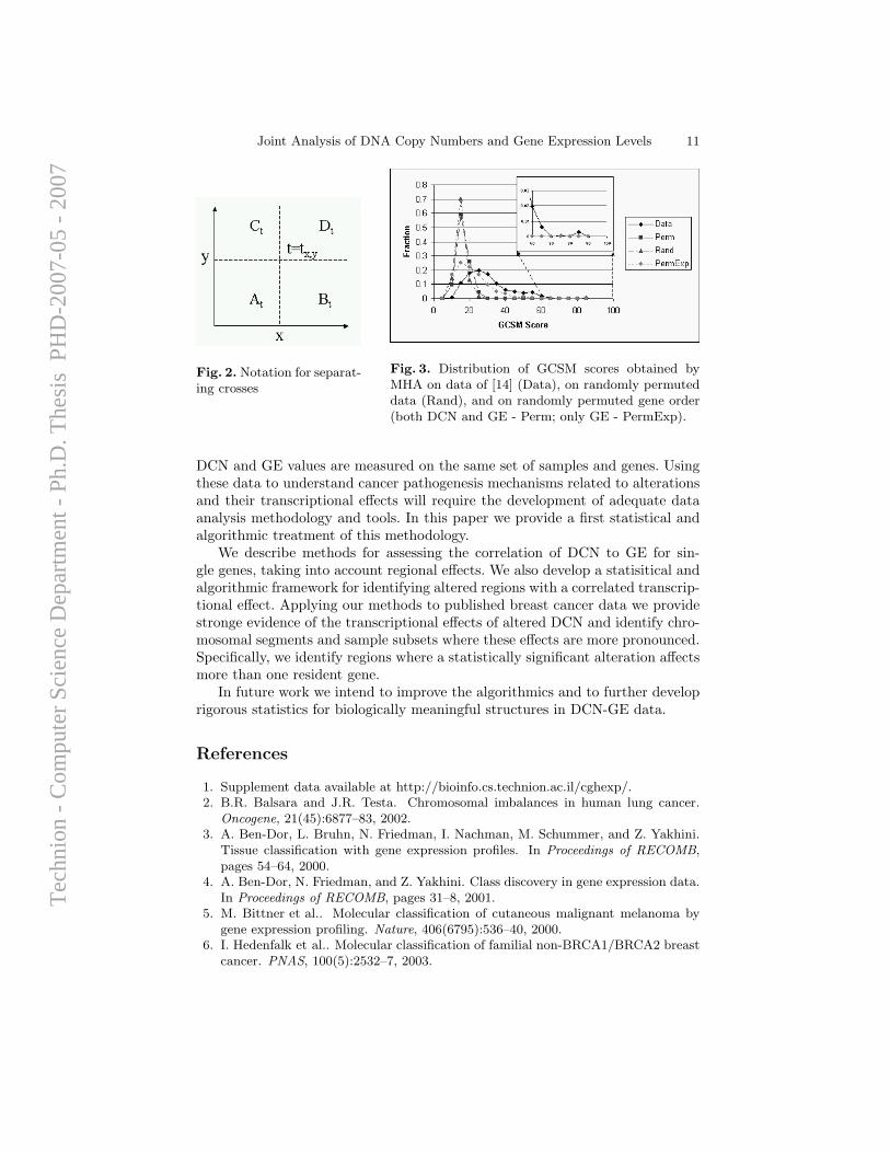
Joint Analysis of DNA Copy Numbers and Gene Expression Levels 11
Fig. 2. Notation for separat-ing crosses
Fig. 3. Distribution of GCSM scores obtained byMHA on data of [14] (Data), on randomly permuteddata (Rand), and on randomly permuted gene order(both DCN and GE - Perm; only GE - PermExp).
DCN and GE values are measured on the same set of samples and genes. Usingthese data to understand cancer pathogenesis mechanisms related to alterationsand their transcriptional effects will require the development of adequate dataanalysis methodology and tools. In this paper we provide a first statistical andalgorithmic treatment of this methodology.
We describe methods for assessing the correlation of DCN to GE for sin-gle genes, taking into account regional effects. We also develop a statisitical andalgorithmic framework for identifying altered regions with a correlated transcrip-tional effect. Applying our methods to published breast cancer data we providestronge evidence of the transcriptional effects of altered DCN and identify chro-mosomal segments and sample subsets where these effects are more pronounced.Specifically, we identify regions where a statistically significant alteration affectsmore than one resident gene.
In future work we intend to improve the algorithmics and to further developrigorous statistics for biologically meaningful structures in DCN-GE data.
References
1. Supplement data available at http://bioinfo.cs.technion.ac.il/cghexp/.2. B.R. Balsara and J.R. Testa. Chromosomal imbalances in human lung cancer.
Oncogene, 21(45):6877–83, 2002.3. A. Ben-Dor, L. Bruhn, N. Friedman, I. Nachman, M. Schummer, and Z. Yakhini.
Tissue classification with gene expression profiles. In Proceedings of RECOMB,pages 54–64, 2000.
4. A. Ben-Dor, N. Friedman, and Z. Yakhini. Class discovery in gene expression data.In Proceedings of RECOMB, pages 31–8, 2001.
5. M. Bittner et al.. Molecular classification of cutaneous malignant melanoma bygene expression profiling. Nature, 406(6795):536–40, 2000.
6. I. Hedenfalk et al.. Molecular classification of familial non-BRCA1/BRCA2 breastcancer. PNAS, 100(5):2532–7, 2003.
Tec
hnio
n -
Com
pute
r Sc
ienc
e D
epar
tmen
t - P
h.D
. The
sis
PH
D-2
007-
05 -
200
7
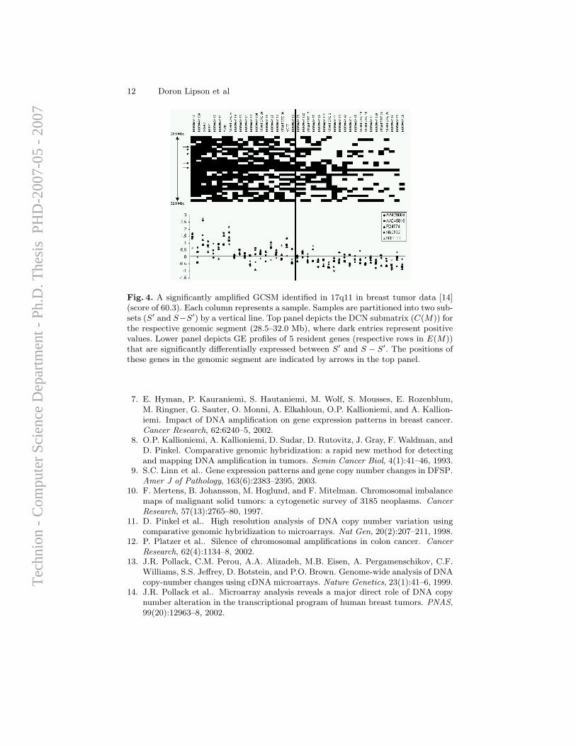
12 Doron Lipson et al
Fig. 4. A significantly amplified GCSM identified in 17q11 in breast tumor data [14](score of 60.3). Each column represents a sample. Samples are partitioned into two sub-sets (S′ and S−S′) by a vertical line. Top panel depicts the DCN submatrix (C(M)) forthe respective genomic segment (28.5–32.0 Mb), where dark entries represent positivevalues. Lower panel depicts GE profiles of 5 resident genes (respective rows in E(M))that are significantly differentially expressed between S′ and S − S′. The positions ofthese genes in the genomic segment are indicated by arrows in the top panel.
7. E. Hyman, P. Kauraniemi, S. Hautaniemi, M. Wolf, S. Mousses, E. Rozenblum,M. Ringner, G. Sauter, O. Monni, A. Elkahloun, O.P. Kallioniemi, and A. Kallion-iemi. Impact of DNA amplification on gene expression patterns in breast cancer.Cancer Research, 62:6240–5, 2002.
8. O.P. Kallioniemi, A. Kallioniemi, D. Sudar, D. Rutovitz, J. Gray, F. Waldman, andD. Pinkel. Comparative genomic hybridization: a rapid new method for detectingand mapping DNA amplification in tumors. Semin Cancer Biol, 4(1):41–46, 1993.
9. S.C. Linn et al.. Gene expression patterns and gene copy number changes in DFSP.Amer J of Pathology, 163(6):2383–2395, 2003.
10. F. Mertens, B. Johansson, M. Hoglund, and F. Mitelman. Chromosomal imbalancemaps of malignant solid tumors: a cytogenetic survey of 3185 neoplasms. CancerResearch, 57(13):2765–80, 1997.
11. D. Pinkel et al.. High resolution analysis of DNA copy number variation usingcomparative genomic hybridization to microarrays. Nat Gen, 20(2):207–211, 1998.
12. P. Platzer et al.. Silence of chromosomal amplifications in colon cancer. CancerResearch, 62(4):1134–8, 2002.
13. J.R. Pollack, C.M. Perou, A.A. Alizadeh, M.B. Eisen, A. Pergamenschikov, C.F.Williams, S.S. Jeffrey, D. Botstein, and P.O. Brown. Genome-wide analysis of DNAcopy-number changes using cDNA microarrays. Nature Genetics, 23(1):41–6, 1999.
14. J.R. Pollack et al.. Microarray analysis reveals a major direct role of DNA copynumber alteration in the transcriptional program of human breast tumors. PNAS,99(20):12963–8, 2002.
Tec
hnio
n -
Com
pute
r Sc
ienc
e D
epar
tmen
t - P
h.D
. The
sis
PH
D-2
007-
05 -
200
7
A.7 Discovering Motifs in Ranked Lists of
DNA Sequences
Eran Eden, Doron Lipson, Sivan Yogev, and Zohar Yakhini. “DiscoveringMotifs in Ranked Lists of DNA Sequences”. PLoS ComputationalBiology, 3(3):e39, 2007.
143
Tec
hnio
n -
Com
pute
r Sc
ienc
e D
epar
tmen
t - P
h.D
. The
sis
PH
D-2
007-
05 -
200
7

144
Tec
hnio
n -
Com
pute
r Sc
ienc
e D
epar
tmen
t - P
h.D
. The
sis
PH
D-2
007-
05 -
200
7
Discovering Motifs in Ranked Lists of DNASequencesEran Eden
1*, Doron Lipson
1, Sivan Yogev
1,2, Zohar Yakhini
1,3*
1 Computer Science Department, Technion, Haifa, Israel, 2 IBM Research Laboratories, Haifa, Israel 3 Agilent Laboratories, Santa Clara, California, United States of America
Computational methods for discovery of sequence elements that are enriched in a target set compared with abackground set are fundamental in molecular biology research. One example is the discovery of transcription factorbinding motifs that are inferred from ChIP–chip (chromatin immuno-precipitation on a microarray) measurements.Several major challenges in sequence motif discovery still require consideration: (i) the need for a principled approachto partitioning the data into target and background sets; (ii) the lack of rigorous models and of an exact p-value formeasuring motif enrichment; (iii) the need for an appropriate framework for accounting for motif multiplicity; (iv) thetendency, in many of the existing methods, to report presumably significant motifs even when applied to randomlygenerated data. In this paper we present a statistical framework for discovering enriched sequence elements in rankedlists that resolves these four issues. We demonstrate the implementation of this framework in a software application,termed DRIM (discovery of rank imbalanced motifs), which identifies sequence motifs in lists of ranked DNA sequences.We applied DRIM to ChIP–chip and CpG methylation data and obtained the following results. (i) Identification of 50novel putative transcription factor (TF) binding sites in yeast ChIP–chip data. The biological function of some of themwas further investigated to gain new insights on transcription regulation networks in yeast. For example, ourdiscoveries enable the elucidation of the network of the TF ARO80. Another finding concerns a systematic TF bindingenhancement to sequences containing CA repeats. (ii) Discovery of novel motifs in human cancer CpG methylationdata. Remarkably, most of these motifs are similar to DNA sequence elements bound by the Polycomb complex thatpromotes histone methylation. Our findings thus support a model in which histone methylation and CpG methylationare mechanistically linked. Overall, we demonstrate that the statistical framework embodied in the DRIM software toolis highly effective for identifying regulatory sequence elements in a variety of applications ranging from expressionand ChIP–chip to CpG methylation data. DRIM is publicly available at http://bioinfo.cs.technion.ac.il/drim.
Citation: Eden E, Lipson D, Yogev S, Yakhini Z (2007) Discovering motifs in ranked lists of DNA sequences. PLoS Comput Biol 3(3): e39. doi:10.1371/journal.pcbi.0030039
Introduction
BackgroundThis paper examines the problem of discovering ‘‘interest-
ing’’ sequence motifs in biological sequence data. A widelyaccepted and more formal definition of this task is: given atarget set and a background set of sequences (or a backgroundmodel), identify sequence motifs that are enriched in the target setcompared with the background set.
The purpose of this paper is to extend this formulation andto make it more flexible so as to enable the determination ofthe target and background set in a data driven manner.
Discovery of sequences or attributes that are enriched in atarget set compared with a background set (or model) hasbecome increasingly useful in a wide range of applications inmolecular biology research. For example, discovery of DNAsequence motifs that are overabundant in a set of promoterregions of co-expressed genes (determined by clustering ofexpression data) can suggest an explanation for this co-expression. Another example is the discovery of DNAsequences that are enriched in a set of promoter regions towhich a certain transcription factor (TF) binds strongly,inferred from chromatin immuno-precipitation on a micro-array (ChIP–chip) [1] measurements. The same principle maybe extended to many other applications such as discovery ofgenomic elements enriched in a set of highly methylated CpGisland sequences [2].
Due to its importance, this task of discovering enrichedDNA subsequences and capturing their corresponding motif
profile has gained much attention in the literature. Anyapproach to motif discovery must address several fundamen-tal issues. The first issue is the way by which motifs arerepresented. There are several strategies for motif represen-tation: using a k-mer of IUPAC symbols where each symbolrepresents a fixed set of possible nucleotides at a singleposition (examples of methods that use this representationinclude REDUCE [3], YMF [4,5], ANN-SPEC [6], and ahypergeometric-based method [7]) or using a position weightmatrix (PWM), which specifies the probability of observingeach nucleotide at each motif position (for example MEME[8], BioProspector [9], MotifBooster [10], DME-X [11], andAlignACE [12]). Both representations assume base positionindependence. Alternatively, higher order representationsthat capture positional dependencies have been proposed
Editor: Ernest Fraenkel, Massachusetts Institute of Technology, United States ofAmerica
Received July 25, 2006; Accepted January 5, 2007; Published March 23, 2007
Copyright: � 2007 Eden et al. This is an open-access article distributed under theterms of the Creative Commons Attribution License, which permits unrestricteduse, distribution, and reproduction in any medium, provided the original authorand source are credited.
Abbreviations: ChIP–chip, chromatin immuno-precipitation on a microarray;DRIM, discovery of rank imbalanced motifs; mDIP, methyl-DNA immunoprecipita-tion; mHG, minimal hypergeometric; OC, other condition; TF, transcription factor;TFBS, transcription factor binding sites; YPD, rich media condition
* To whom correspondence should be addressed. E-mail: [email protected] or [email protected] (EE), [email protected] (ZY)
PLoS Computational Biology | www.ploscompbiol.org March 2007 | Volume 3 | Issue 3 | e390001
Tec
hnio
n -
Com
pute
r Sc
ienc
e D
epar
tmen
t - P
h.D
. The
sis
PH
D-2
007-
05 -
200
7
(e.g., HMM and Bayesian networks motif representations[13]). While these representations circumvent the positionindependence assumption, they are more vulnerable tooverfitting and lack of data for determining model param-eters. The method described in this paper uses the k-mermodel with symbols above IUPAC.
The second issue is devising a motif scoring scheme. Manystrategies for scoring motifs have been suggested in theliterature. One simple yet powerful approach uses thehypergeometric distribution for identifying enriched motifkernels in a set of sequences and then expanding these motifsusing an EM algorithm [7]. The framework described in thispaper is a natural extension of the approach of [7]. YMF [4,5]is an exhaustive search algorithm which associates each motifwith a z-score. AlignACE [12] uses a Gibbs sampling algorithmfor finding global sequence alignments and produces a MAPscore. This score is an internal metric used to determine thesignificance of an alignment. MEME [8] uses an expectationmaximization strategy and outputs the log-likelihood andrelative entropy associated with each motif.
Once a scoring scheme is devised, a defined motif searchspace is scanned (either heuristically or exhaustively) andmotifs with significantly high scores are identified. Todetermine the statistical significance of the obtained scores,many methods resort to simulations or ad hoc thresholds.Several excellent reviews narrate the different strategies formotif detection and use quantitative benchmarking tocompare their performance [14–18]. A related aspect ofmotif discovery, which is outside the scope of this paper,focuses on properties of clusters and modules of TF bindingsites (TFBS). Examples of approaches that search forcombinatorial patterns and modules underlying TF bindingand gene expression include [19–23].
Open Challenges in Motif DiscoveryOne issue of motif discovery that is often overlooked
concerns the partition of the input set of sequences into target
and background sets. Many methods rely on the user to providethese two sets and search for motifs that are overabundant inthe former set compared with the latter. The question of howto partition the data into target and background sets is left tothe user. However, the boundary between the sets is oftenunclear and the exact choice of sequences in each setarbitrary. For example, suppose that one wishes to identifymotifs within promoter sequences that constitute putativeTFBS. An obvious strategy would be to partition the set ofpromoter sequences into target and background sets accord-ing to the TF binding signal (as measured by ChIP–chipexperiments). The two sets would contain the sequences towhich the TF binds ‘‘strongly’’ and ‘‘weakly,’’ respectively. Amotif detection algorithm could then be applied to findmotifs that are overabundant in the target set compared withthe background set. In this scenario, the positioning of thecutoff between the strong and weak binding signal issomewhat arbitrary. Obviously, the final outcome of themotif identification process can be highly dependent on thischoice of cutoff. A stringent cutoff will result in the exclusionof informative sequences from the target set while apromiscuous cutoff will cause inclusion of nonrelevantsequences—both extremes hinder the accuracy of motifprediction. This example demonstrates a fundamental diffi-culty in partitioning most types of data. Several methodsattempt to circumvent this hurdle. For example, REDUCE [3]uses a regression model on the entire set of sequences.However, it is difficult to justify this model in the context ofmultiple motif occurrence (as explained below). In otherwork, a variant of the Kolmogorov-Smirnov test was used formotif discovery [24]. This approach successfully circumventsarbitrary data partition. However, it has other limitationssuch as the failure to address multiple motif occurrences in asingle promoter, and the lack of an exact characterization ofthe null distribution. Overall, the following four majorchallenges in motif discovery still require consideration: (c1)the cutoff used to partition data into a target set andbackground set of sequences is often chosen arbitrarily; (c2)lack of an exact statistical score and p-value for motifenrichment. Current methods typically use arbitrarily setthresholds or simulations, which are inherently limited inprecision and costly in terms of running time; (c3) a need foran appropriate framework that accounts for multiple motifoccurrences in a single promoter. For example, how shouldone quantify the significance of a single motif occurrence in apromoter against two motif occurrences in a promoter?Linear models [3] assume that the weight of the latter isdouble that of the former. However, it is difficult to justifythis approach since biological systems do not necessarilyoperate in such a linear fashion. Another issue related tomotif multiplicity is low complexity or repetitive regions.These regions often contain multiple copies of degeneratemotifs (e.g., CA repeats). Since the nucleotide frequencyunderlying these regions substantially deviates from thestandard background frequency, they often cause false-motifdiscoveries. Consequently, most methods mask these regionsin the preprocessing stage and thereby lose vital informationthat might reside therein; (c4) criticism has been made overthe fact that motif discovery methods tend to reportpresumably significant motifs even when applied on ran-domly generated data [25]. These motifs are clear cases offalse positives and should be avoided.
PLoS Computational Biology | www.ploscompbiol.org March 2007 | Volume 3 | Issue 3 | e390002
Author Summary
A computational problem with many applications in molecularbiology is to identify short DNA sequence patterns (motifs) that aresignificantly overrepresented in a target set of genomic sequencesrelative to a background set of genomic sequences. One example isa target set that contains DNA sequences to which a specifictranscription factor protein was experimentally measured as boundwhile the background set contains sequences to which the sametranscription factor was not bound. Overrepresented sequencemotifs in the target set may represent a subsequence that ismolecularly recognized by the transcription factor. An inherentlimitation of the above formulation of the problem lies in the factthat in many cases data cannot be clearly partitioned into distincttarget and background sets in a biologically justified manner. Wedescribe a statistical framework for discovering motifs in a list ofgenomic sequences that are ranked according to a biologicalparameter or measurement (e.g., transcription factor to sequencebinding measurements). Our approach circumvents the need topartition the data into target and background sets using arbitrarilyset parameters. The framework is implemented in a software toolcalled DRIM. The application of DRIM led to the identification ofnovel putative transcription factor binding sites in yeast and to thediscovery of previously unknown motifs in CpG methylation regionsin human cancer cell lines.
Discovering Motifs in Ranked ListsT
echn
ion
- C
ompu
ter
Scie
nce
Dep
artm
ent -
Ph.
D. T
hesi
s P
HD
-200
7-05
- 2
007
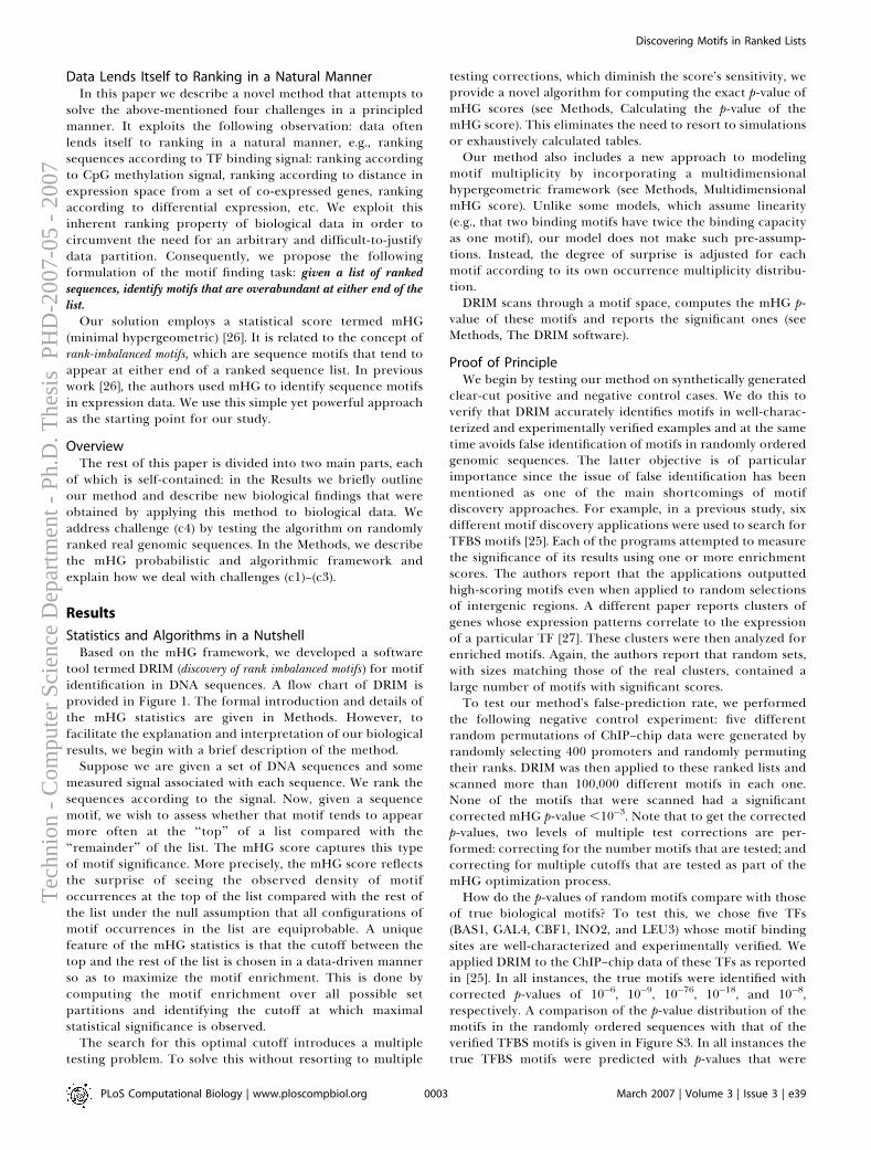
Data Lends Itself to Ranking in a Natural MannerIn this paper we describe a novel method that attempts to
solve the above-mentioned four challenges in a principledmanner. It exploits the following observation: data oftenlends itself to ranking in a natural manner, e.g., rankingsequences according to TF binding signal: ranking accordingto CpG methylation signal, ranking according to distance inexpression space from a set of co-expressed genes, rankingaccording to differential expression, etc. We exploit thisinherent ranking property of biological data in order tocircumvent the need for an arbitrary and difficult-to-justifydata partition. Consequently, we propose the followingformulation of the motif finding task: given a list of rankedsequences, identify motifs that are overabundant at either end of thelist.
Our solution employs a statistical score termed mHG(minimal hypergeometric) [26]. It is related to the concept ofrank-imbalanced motifs, which are sequence motifs that tend toappear at either end of a ranked sequence list. In previouswork [26], the authors used mHG to identify sequence motifsin expression data. We use this simple yet powerful approachas the starting point for our study.
OverviewThe rest of this paper is divided into two main parts, each
of which is self-contained: in the Results we briefly outlineour method and describe new biological findings that wereobtained by applying this method to biological data. Weaddress challenge (c4) by testing the algorithm on randomlyranked real genomic sequences. In the Methods, we describethe mHG probabilistic and algorithmic framework andexplain how we deal with challenges (c1)–(c3).
Results
Statistics and Algorithms in a NutshellBased on the mHG framework, we developed a software
tool termed DRIM (discovery of rank imbalanced motifs) for motifidentification in DNA sequences. A flow chart of DRIM isprovided in Figure 1. The formal introduction and details ofthe mHG statistics are given in Methods. However, tofacilitate the explanation and interpretation of our biologicalresults, we begin with a brief description of the method.
Suppose we are given a set of DNA sequences and somemeasured signal associated with each sequence. We rank thesequences according to the signal. Now, given a sequencemotif, we wish to assess whether that motif tends to appearmore often at the ‘‘top’’ of a list compared with the‘‘remainder’’ of the list. The mHG score captures this typeof motif significance. More precisely, the mHG score reflectsthe surprise of seeing the observed density of motifoccurrences at the top of the list compared with the rest ofthe list under the null assumption that all configurations ofmotif occurrences in the list are equiprobable. A uniquefeature of the mHG statistics is that the cutoff between thetop and the rest of the list is chosen in a data-driven mannerso as to maximize the motif enrichment. This is done bycomputing the motif enrichment over all possible setpartitions and identifying the cutoff at which maximalstatistical significance is observed.
The search for this optimal cutoff introduces a multipletesting problem. To solve this without resorting to multiple
testing corrections, which diminish the score’s sensitivity, weprovide a novel algorithm for computing the exact p-value ofmHG scores (see Methods, Calculating the p-value of themHG score). This eliminates the need to resort to simulationsor exhaustively calculated tables.Our method also includes a new approach to modeling
motif multiplicity by incorporating a multidimensionalhypergeometric framework (see Methods, MultidimensionalmHG score). Unlike some models, which assume linearity(e.g., that two binding motifs have twice the binding capacityas one motif), our model does not make such pre-assump-tions. Instead, the degree of surprise is adjusted for eachmotif according to its own occurrence multiplicity distribu-tion.DRIM scans through a motif space, computes the mHG p-
value of these motifs and reports the significant ones (seeMethods, The DRIM software).
Proof of PrincipleWe begin by testing our method on synthetically generated
clear-cut positive and negative control cases. We do this toverify that DRIM accurately identifies motifs in well-charac-terized and experimentally verified examples and at the sametime avoids false identification of motifs in randomly orderedgenomic sequences. The latter objective is of particularimportance since the issue of false identification has beenmentioned as one of the main shortcomings of motifdiscovery approaches. For example, in a previous study, sixdifferent motif discovery applications were used to search forTFBS motifs [25]. Each of the programs attempted to measurethe significance of its results using one or more enrichmentscores. The authors report that the applications outputtedhigh-scoring motifs even when applied to random selectionsof intergenic regions. A different paper reports clusters ofgenes whose expression patterns correlate to the expressionof a particular TF [27]. These clusters were then analyzed forenriched motifs. Again, the authors report that random sets,with sizes matching those of the real clusters, contained alarge number of motifs with significant scores.To test our method’s false-prediction rate, we performed
the following negative control experiment: five differentrandom permutations of ChIP–chip data were generated byrandomly selecting 400 promoters and randomly permutingtheir ranks. DRIM was then applied to these ranked lists andscanned more than 100,000 different motifs in each one.None of the motifs that were scanned had a significantcorrected mHG p-value ,10�3. Note that to get the correctedp-values, two levels of multiple test corrections are per-formed: correcting for the number motifs that are tested; andcorrecting for multiple cutoffs that are tested as part of themHG optimization process.How do the p-values of random motifs compare with those
of true biological motifs? To test this, we chose five TFs(BAS1, GAL4, CBF1, INO2, and LEU3) whose motif bindingsites are well-characterized and experimentally verified. Weapplied DRIM to the ChIP–chip data of these TFs as reportedin [25]. In all instances, the true motifs were identified withcorrected p-values of 10�6, 10�9, 10�76, 10�18, and 10�8,respectively. A comparison of the p-value distribution of themotifs in the randomly ordered sequences with that of theverified TFBS motifs is given in Figure S3. In all instances thetrue TFBS motifs were predicted with p-values that were
PLoS Computational Biology | www.ploscompbiol.org March 2007 | Volume 3 | Issue 3 | e390003
Discovering Motifs in Ranked ListsT
echn
ion
- C
ompu
ter
Scie
nce
Dep
artm
ent -
Ph.
D. T
hesi
s P
HD
-200
7-05
- 2
007
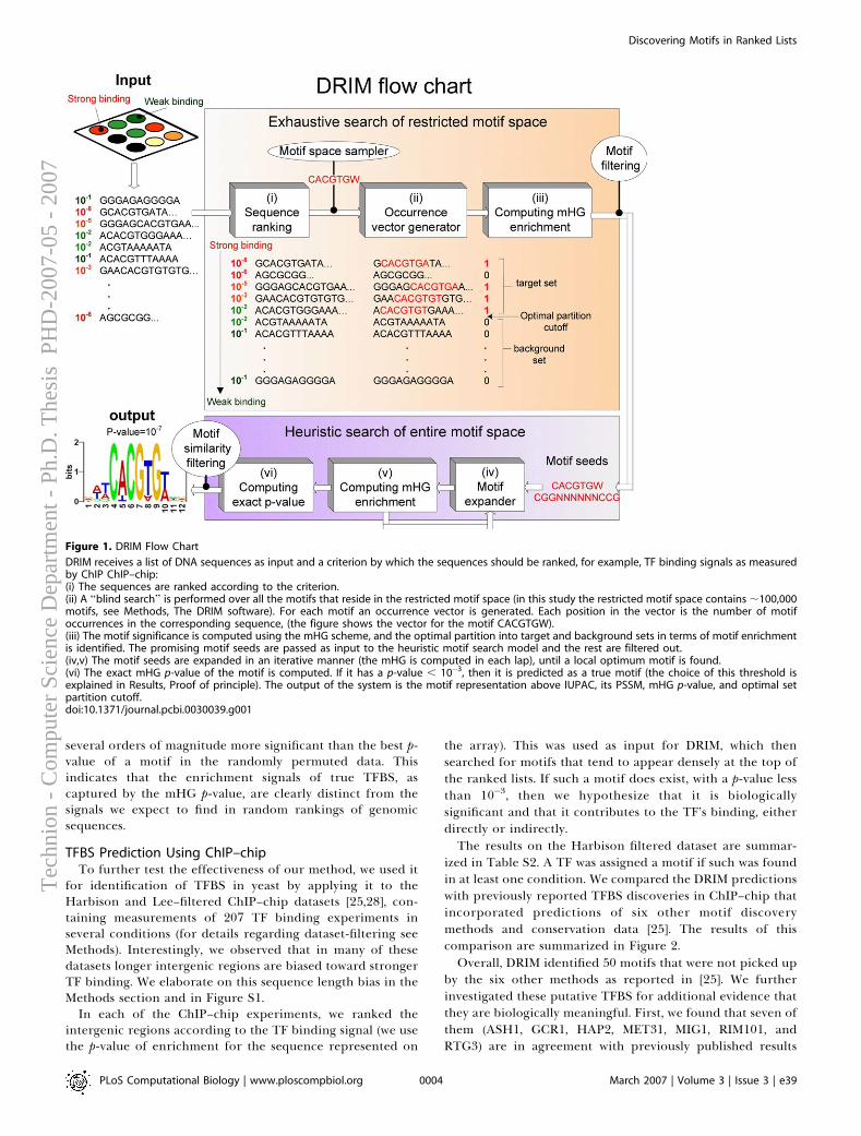
several orders of magnitude more significant than the best p-value of a motif in the randomly permuted data. Thisindicates that the enrichment signals of true TFBS, ascaptured by the mHG p-value, are clearly distinct from thesignals we expect to find in random rankings of genomicsequences.
TFBS Prediction Using ChIP–chipTo further test the effectiveness of our method, we used it
for identification of TFBS in yeast by applying it to theHarbison and Lee–filtered ChIP–chip datasets [25,28], con-taining measurements of 207 TF binding experiments inseveral conditions (for details regarding dataset-filtering seeMethods). Interestingly, we observed that in many of thesedatasets longer intergenic regions are biased toward strongerTF binding. We elaborate on this sequence length bias in theMethods section and in Figure S1.
In each of the ChIP–chip experiments, we ranked theintergenic regions according to the TF binding signal (we usethe p-value of enrichment for the sequence represented on
the array). This was used as input for DRIM, which thensearched for motifs that tend to appear densely at the top ofthe ranked lists. If such a motif does exist, with a p-value lessthan 10�3, then we hypothesize that it is biologicallysignificant and that it contributes to the TF’s binding, eitherdirectly or indirectly.The results on the Harbison filtered dataset are summar-
ized in Table S2. A TF was assigned a motif if such was foundin at least one condition. We compared the DRIM predictionswith previously reported TFBS discoveries in ChIP–chip thatincorporated predictions of six other motif discoverymethods and conservation data [25]. The results of thiscomparison are summarized in Figure 2.Overall, DRIM identified 50 motifs that were not picked up
by the six other methods as reported in [25]. We furtherinvestigated these putative TFBS for additional evidence thatthey are biologically meaningful. First, we found that seven ofthem (ASH1, GCR1, HAP2, MET31, MIG1, RIM101, andRTG3) are in agreement with previously published results
Figure 1. DRIM Flow Chart
DRIM receives a list of DNA sequences as input and a criterion by which the sequences should be ranked, for example, TF binding signals as measuredby ChIP ChIP–chip:(i) The sequences are ranked according to the criterion.(ii) A ‘‘blind search’’ is performed over all the motifs that reside in the restricted motif space (in this study the restricted motif space contains ;100,000motifs, see Methods, The DRIM software). For each motif an occurrence vector is generated. Each position in the vector is the number of motifoccurrences in the corresponding sequence, (the figure shows the vector for the motif CACGTGW).(iii) The motif significance is computed using the mHG scheme, and the optimal partition into target and background sets in terms of motif enrichmentis identified. The promising motif seeds are passed as input to the heuristic motif search model and the rest are filtered out.(iv,v) The motif seeds are expanded in an iterative manner (the mHG is computed in each lap), until a local optimum motif is found.(vi) The exact mHG p-value of the motif is computed. If it has a p-value , 10�3, then it is predicted as a true motif (the choice of this threshold isexplained in Results, Proof of principle). The output of the system is the motif representation above IUPAC, its PSSM, mHG p-value, and optimal setpartition cutoff.doi:10.1371/journal.pcbi.0030039.g001
PLoS Computational Biology | www.ploscompbiol.org March 2007 | Volume 3 | Issue 3 | e390004
Discovering Motifs in Ranked ListsT
echn
ion
- C
ompu
ter
Scie
nce
Dep
artm
ent -
Ph.
D. T
hesi
s P
HD
-200
7-05
- 2
007
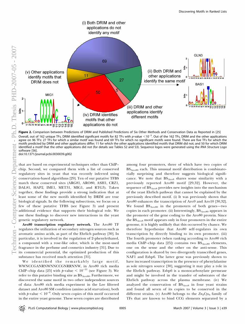
that are based on experimental techniques other than ChIP–chip. Second, we compared them with a list of conservedregulatory sites in yeast that was recently inferred usingconservation-based algorithms [29]. Ten of our putative TFBSmatch these conserved sites (ARG81, ARO80, ASH1, CRZ1,DAL81, HAP2, IME1, MET31, MIG1, and RTG3). Takentogether, these findings provide a strong indication that atleast some of the new motifs identified by DRIM are truebiological signals. In the following subsections, we focus on afew of these putative TFBS (see Figure 3) and presentadditional evidence that supports their biological role. Weuse these findings to discover new interactions in the yeastgenetic regulatory network.
Aro80 transcription regulatory network. The Aro80 TFregulates the utilization of secondary nitrogen sources such asaromatic amino acids, as part of the Ehrlich pathway [30]. Inparticular, it is involved in the regulation of 2-phenylethanol,a compound with a rose-like odor, which is the most-usedfragrance in the perfume and cosmetics industry [31]. Due toits commercial potential, the optimized production of thissubstance has received much attention [31].
We id en t i fi ed the r emarkab l y l a r g e mo t i f ,WWNCCGANRNWNNCCGNRRNNW, in Aro80 rich mediaChIP–chip data [25] with p-value , 10�11 (see Figure 3). Werefer to this putative binding site as BSAro80. Furthermore, wediscovered the same motif in two other independent sourcesof data: Aro80 rich media experiment in the Lee filtereddataset and Aro80 SM condition (amino acid starvation), bothwith p-value , 10�6. Only seven copies of this motif occurredin the entire yeast genome. These seven copies are distributed
among four promoters, three of which have two copies ofBSAro80 each. This unusual motif distribution is combinato-rially surprising and therefore suggests biological signifi-cance. We note that BSAro8 shares some similarity with apreviously reported Aro80 motif [29,32]. However, thesequence of BSAro8 provides new insights into the mechanismof the yeast Ehrlich pathway that cannot be explained by thepreviously described motif. (i) It was previously shown thatAro80 enhances the transcription of Aro9 and Aro10 [30,32].We found BSAro80 in the promoters of both genes—twocopies in each promoter. (ii) Interestingly, BSAro80 appears inthe promoter of the gene coding to the Aro80 protein. Sincethe BSAro8 motif appears only in four promoters in the entiregenome, it is highly unlikely that this occurred by chance. Wetherefore hypothesize that Aro80 self-regulates its owntranscription by directly binding to its own promoter. (iii)The fourth promoter (when ranking according to Aro80 richmedia ChIP–chip data [25]) contains two BSAro80 elements,one on the sense and the other on the anti-sense. Thisconfiguration is shared by two divergently transcribed genes,NAF1 and Esbp6. The latter gene was previously shown tohave increased transcription in the presence of phenylalanineas sole nitrogen source [30], suggesting it may play a role inthe Ehrlich pathway. Esbp6 is a monocarboxylate permeaseand might be involved in the transfer of substrates of theEhrlich pathway across the plasma membrane. (iv) Weanalyzed the conservation of BSAro8 in four yeast strainsand found all seven of its copies to be conserved in thedifferent strains. (v) Aro80 belongs to the Zn2Cys6 family ofTFs that are known to bind CCG elements separated by a
Figure 2. Comparison between Predictions of DRIM and Published Predictions of Six Other Methods and Conservation Data as Reported in [25]
Overall, out of 162 unique TFs, DRIM identified significant motifs for 82 TFs with p-value ,10�3. Out of the 162 TFs, DRIM and the other applicationsagree on 96 TFs: 27 TFs for which a similar motif was found and 69 TFs for which no significant motifs were found. There are five TFs for which themotifs predicted by DRIM and other applications differ; 11 for which the other applications identified motifs that DRIM did not; and 50 for which DRIMidentified a motif that the other applications did not (for details see Tables S2 and S3). Sequence logos were generated using the RNA Structure Logosoftware [56].doi:10.1371/journal.pcbi.0030039.g002
PLoS Computational Biology | www.ploscompbiol.org March 2007 | Volume 3 | Issue 3 | e390005
Discovering Motifs in Ranked ListsT
echn
ion
- C
ompu
ter
Scie
nce
Dep
artm
ent -
Ph.
D. T
hesi
s P
HD
-200
7-05
- 2
007

spacing. Indeed, in addition to other conserved nucleotides,the motif contains CCG gapped tri-nucleotides. (vi) In aprevious study, in order to identify cis-acting sequencesinvolved in Aro9 induction, a series of deletions wereproduced in the Aro9 promoter region, and the expressionof a reporter gene was monitored [32]. The authorsconcluded that the sequence CCGN7CCGN7CCGN7CCG inthe Aro9 promoter is responsible for Aro80 binding. Wenote, however, that the changes in expression caused by themutations can be interpreted differently, and in fact they areeven more consistent with our BSAro80 motif. Deletions ormutations that simultaneously altered all motif copies in thepromoter dramatically reduced expression, while those whichaltered only some of the copies caused a more mild decrease.Other deletions that did not affect any BSAro80 motif did notaffect the expression at all. A detailed analysis of the BSAro80element with respect to these mutagenesis studies is given inFigure S4.
A putative transcription network of Aro80 that incorpo-rates these findings is shown in Figure 4. Note that GATAbinding sites are found adjacent to the BSAro80 motif. Wefurther discuss the potential role of these motifs in theDiscussion.
The predicted motif BSAro80 exemplifies the usefulness ofthe mHG flexible cutoff. Our process partitioned the datainto a target set containing the top first four promoters (theonly promoters in the genome in which the motif resides) anda background set containing the rest of the promoters. Othermethods that used a fixed binding signal cutoff (p-value ,
10�3) for partitioning the data included 16 other promotersin the target set, in addition to the four promoters in whichBSAro80 appears. Consequentially, the signal-to-noise ratiodecreases, which might explain why other methods did notidentify the BSAro80 element.Taken together, our results suggest the predicted BSAro80
motif is indeed an Aro80 binding site.CA repeats are correlated with TF binding. We identified a
bi-nucleotide CA repeat motif with variable length rangingfrom six to 62 in the Harbison filtered dataset. The CA repeatmotif was found to be highly enriched for seven TFs: ARR1,GCR2, IME4, and ACE2 in rich media condition and AFT2,MAL33, and SFP1 in H2O2Hi condition. Furthermore, for twoof these TFs (GCR2, IME4), we rediscovered the same CArepeat motif in the Lee filtered dataset. In other words, forthe specified TFs, we identify a highly significant correlationbetween a sequence’s capacity to bind the TF and thepresence of a CA repeat in the sequence. This type of lowcomplexity motifs are often filtered by current methods. Oneexception is a recent work in which a CACACACACACsequence was found to be enriched in Rap1 experiments [33].It has been previously hypothesized that CA repeats might
have a functional role in TF binding [34]. It was proposed thatCA repeats, which are often conserved in evolutionary distantorganisms, are likely to impose a unique DNA tertiarystructure that aids in the identification of other specificregulatory elements [34]. Our findings constitute concreteevidence to this phenomena in seven (of 82) different TFs.They are also in agreement with another study in which CA
Figure 3. Examples of TFs for Which DRIM Identifies Novel Motifs
We further investigated these motifs and show evidence of their biological function. YPD, H2O2, and SM denote the ChIP–chip experimental conditions[25] in which the motifs were identified.doi:10.1371/journal.pcbi.0030039.g003
PLoS Computational Biology | www.ploscompbiol.org March 2007 | Volume 3 | Issue 3 | e390006
Discovering Motifs in Ranked ListsT
echn
ion
- C
ompu
ter
Scie
nce
Dep
artm
ent -
Ph.
D. T
hesi
s P
HD
-200
7-05
- 2
007
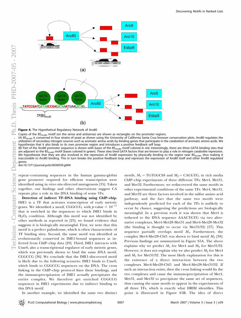
repeat–containing sequences in the human gamma-globingene promoter required for efficient transcription wereidentified using in vitro site-directed mutagenesis [35]. Takentogether, our findings and other observations suggest CArepeats play a role in the DNA binding of some TFs.
Detection of indirect TF–DNA binding using ChIP–chip.IME1 is a TF that activates transcription of early meioticgenes. We identified a motif, CGGCCG, with p-value , 10�11
that is enriched in the sequences to which IME1 binds inH2O2 condition. Although this motif was not identified byother methods as reported in [25], we found evidence thatsuggests it is biologically meaningful. First, we note that thismotif is a perfect palindrome, which is often characteristic ofTF binding sites. Second, the same motif was identified asevolutionarily conserved in IME1-bound sequences as in-ferred from ChIP–chip data [29]. Third, IME1 interacts withUme6, also a transcriptional regulator of early meiotic genes,which was previously shown to bind the same DNA motif,CGGCCG [36]. We conclude that the IME1-discovered motifis likely due to the following scenario: IME1 binds to Ume6,which binds to CGGCCG sequences on the DNA. The crosslinking in the ChIP–chip protocol fixes these bindings, andthe immunoprecipitation of IME1 actually precipitates theentire complex. We therefore get enriched CGGCCGsequences in IME1 experiments due to indirect binding tothis DNA motif.
In another example, we identified the same two distinct
motifs, M1 ¼ TGTGGCSS and M2 ¼ CACGTG, in rich mediaChIP–chip experiments of three different TFs: Met4, Met31,and Met32. Furthermore, we rediscovered the same motifs inother experimental conditions of the same TFs. Met4, Met31,and Met32 are three factors involved in the sulfur amino acidpathway, and the fact that the same two motifs wereindependently predicted for each of the TFs is unlikely tooccur by chance, suggesting the predictions are biologicallymeaningful. In a previous work it was shown that Met4 istethered to the DNA sequence AAACTGTG via two alter-native complexes, Met4-Met28-Met31 and Met4-Met28-Met32(the binding is thought to occur via Met31/32) [37]. Thissequence partially overlaps motif M1. Furthermore, thecomplex Met4-Met28-Cbf1 was shown to bind motif M2 [38].Previous findings are summarized in Figure S5A. The aboveexplains why we predict M1 for Met4 and M2 for Met31/32.However, it does not explain why we also predict M2 for Met4and M1 for Met31/32. The most likely explanation for this isthe existence of a direct interaction between the twocomplexes Met4-Met28-Cbf1 and Met4-Met28-Met31/32. Ifsuch an interaction exists, then the cross linking would fix thetwo complexes and cause the immunoprecipitation of Met4,Met31, and Met32 to precipitate the same set of sequences,thus causing the same motifs to appear in the experiments ofall three TFs, which is exactly what DRIM identifies. Thispoint is illustrated in Figure S5B. The idea of direct
Figure 4. The Hypothetical Regulatory Network of Aro80
Copies of the BSAro80 motif (on the sense and antisense) are shown as rectangles on the promoter regions.(A) BSAro80 is conserved in four strains of yeast as shown using the University of California Santa Cruz browser conservation plots. Aro80 regulates theutilization of secondary nitrogen sources such as aromatic amino acids by binding genes that participate in the catabolism of aromatic amino acids. Wehypothesize that it also binds to its own promoter region and introduces a positive feedback self loop.(B) Part of the Aro80 promoter sequence is shown with bases of the BSAro80 motif colored in red. Interestingly, there are three GATA binding sites thatare adjacent to the BSAro80 motif (bases colored in green). These sites bind GATA factors that are known to play a role in nitrogen catabolite repression.We hypothesize that they are also involved in the repression of Aro80 expression by physically binding to the region near BSAro80, thus making itinaccessible to Aro80 binding. This in turn breaks the positive feedback loop and represses the expression of Aro80 itself and other Aro80 regulatedgenes.doi:10.1371/journal.pcbi.0030039.g004
PLoS Computational Biology | www.ploscompbiol.org March 2007 | Volume 3 | Issue 3 | e390007
Discovering Motifs in Ranked ListsT
echn
ion
- C
ompu
ter
Scie
nce
Dep
artm
ent -
Ph.
D. T
hesi
s P
HD
-200
7-05
- 2
007
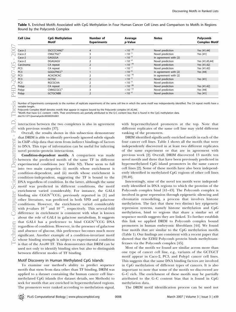
interaction between the two complexes is also in agreementwith previous results [37].
Overall, the results shown in this subsection demonstratethat DRIM is able to identify previously ignored subtle signalsin ChIP–chip data that stem from indirect bindings of factorsto DNA. This type of information can be useful for inferringnovel protein–protein interactions.
Condition-dependent motifs. A comparison was madebetween the predicted motifs of the same TF in differentexperimental conditions (see Table S2). These seem to fallinto two main categories: (i) motifs whose enrichment iscondition-dependent, and (ii) motifs whose enrichment iscondition-independent, suggesting the TF is bound to theDNA regardless of condition. In the latter, although the samemotif was predicted in different conditions, the motifenrichment varied considerably. For instance, the GAL4binding site CGGN11CCG, previously reported in [1] andother literature, was predicted in both YPD and galactoseconditions. However, the enrichment varied considerablywith p-values 10�7 and 10�11, respectively. This several-folddifference in enrichment is consistent with what is knownabout the role of GAL4 in galactose metabolism. It suggeststhat GAL4 has a preference to bind CGGN11CCG DNAregardless of condition. However, in the presence of galactoseand absence of glucose, this preference becomes much moresignificant. Another example of a condition-invariant motifwhose binding strength is subject to experimental conditionis that of the Aro80 TF. This demonstrates that DRIM can beused not only to identify binding sites but also to distinguishbetween different modes of TF binding.
Motif Discovery in Human Methylated CpG IslandsTo examine our method’s ability to predict sequence
motifs that stem from data other than TF binding, DRIM wasapplied to a dataset containing the human cancer cell line–methylated CpG islands (for dataset details, see Methods) toseek for motifs that are enriched in hypermethylated regions.The promoters were ranked according to methylation signal,
with hypermethylated promoters at the top. Note thatdifferent replicates of the same cell line may yield differentranking of the promoters.DRIM identified significantly enriched motifs in each of the
four cancer cell lines. Table 1 shows all the motifs that wereindependently discovered in at least two different replicatesof the same experiment or that are in agreement withprevious work [2]. Overall, DRIM discovered 13 motifs: tennovel motifs and three that have been previously predicted inhypermethylated CpG island promoters in the same cancercell lines [2]. Some of these motifs have also been independ-ently identified in methylated CpG regions of other cell lines[39,40].Interestingly, nine of the novel ten motifs were independ-
ently identified in DNA regions to which the proteins of thePolycomb complex bind [41–43]. The Polycomb complex isinvolved in gene repression through epigenetic silencing andchromatin remodeling, a process that involves histonemethylation. The fact that these two distinct key epigeneticrepression systems, namely histone methylation and CpGmethylation, bind to regions that share a similar set ofsequence motifs suggests they are linked. To further establishthis link we applied DRIM to Polycomb complex boundpromoters in human embryonic fibroblasts [44]. We foundfour motifs that are similar to the CpG methylation motifs(Table 1). Our findings are consistent with a recent paper thatshowed that the EZH2 Polycomb protein binds methyltrans-ferases via the Polycomb complex [45].Most of the motifs we found are similar across more than
one type of cancer cell line, e.g., variants of the GCTGCTmotif appear in Caco-2, PC3, and Polyp1 cancer cell lines.This suggests that the same DNA binding factors are involvedin CpG methylation of different types of cancers. It is alsoimportant to note that some of the motifs we discovered areG–C rich. The enrichment of these motifs may be partiallyattributed to the G–C content bias that is found in CpGmethylation data.The DRIM motif identification process can be used not
Table 1. Enriched Motifs Associated with CpG Methylation in Four Human Cancer Cell Lines and Comparison to Motifs in RegionsBound by the Polycomb Complex
Cell Line CpG Methylation
Motif
Number of
Experiments
Average
p-Value
Notes Polycomb
Complex Motif
Caco-2 SSCCCCANGa 4 ,10�10 Novel prediction Yes [41,44]
Caco-2 CNGCTGCa 3 ,10�5 Novel prediction Yes [41]
Caco-2 GAGGGA 2 ,10�4 In agreement with [2]
Caco-2 DGAGAGV 2 ,10�4 Novel prediction Yes [41,43,44]
Carcinoma CA repeat 2 ,10�79 Novel prediction Yes [41,42]
PC3 CA repeat 1 ,10�7 Novel prediction Yes [41,42]
PC3 GGGGTNCCa 1 ,10�6 In agreement with [2] Yes [44]
PC3 ACACNCAC 2 ,10�10 In agreement with [2]
PC3 GCTGC 2 ,10�5 Novel prediction Yes [41]
PC3 RGCGCAA 2 ,10�4 Novel prediction
Polyp CA repeat 2 ,10�58 Novel prediction Yes [41,42]
Polyp CNNGCGCCa 3 ,10�13 Novel prediction Yes [44]
Polyp GCTGCNBB 2 ,10�6 Novel prediction Yes [41]
Number of Experiments corresponds to the number of replicate experiments of the same cell line in which the same motif was independently identified. The CA repeat motifs have avariable length.Polycomb Complex Motif denotes motifs that appear in regions bound by the Polycomb complex [41,42,44].aMotifs that have G-C content .66%. Their enrichments are partially attributed to the G-C content bias that is found in the CpG methylation data.doi:10.1371/journal.pcbi.0030039.t001
PLoS Computational Biology | www.ploscompbiol.org March 2007 | Volume 3 | Issue 3 | e390008
Discovering Motifs in Ranked ListsT
echn
ion
- C
ompu
ter
Scie
nce
Dep
artm
ent -
Ph.
D. T
hesi
s P
HD
-200
7-05
- 2
007
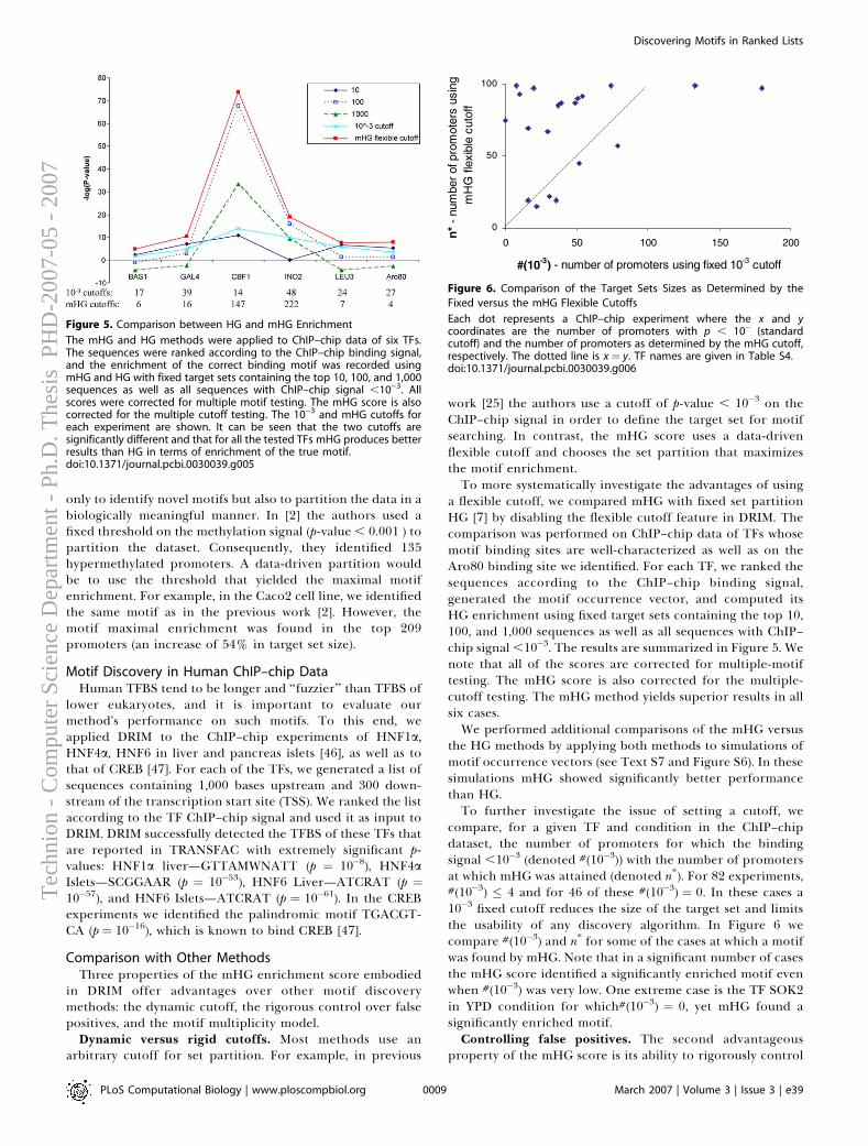
only to identify novel motifs but also to partition the data in abiologically meaningful manner. In [2] the authors used afixed threshold on the methylation signal (p-value , 0.001 ) topartition the dataset. Consequently, they identified 135hypermethylated promoters. A data-driven partition wouldbe to use the threshold that yielded the maximal motifenrichment. For example, in the Caco2 cell line, we identifiedthe same motif as in the previous work [2]. However, themotif maximal enrichment was found in the top 209promoters (an increase of 54% in target set size).
Motif Discovery in Human ChIP–chip DataHuman TFBS tend to be longer and ‘‘fuzzier’’ than TFBS of
lower eukaryotes, and it is important to evaluate ourmethod’s performance on such motifs. To this end, weapplied DRIM to the ChIP–chip experiments of HNF1a,HNF4a, HNF6 in liver and pancreas islets [46], as well as tothat of CREB [47]. For each of the TFs, we generated a list ofsequences containing 1,000 bases upstream and 300 down-stream of the transcription start site (TSS). We ranked the listaccording to the TF ChIP–chip signal and used it as input toDRIM. DRIM successfully detected the TFBS of these TFs thatare reported in TRANSFAC with extremely significant p-values: HNF1a liver—GTTAMWNATT (p ¼ 10�8), HNF4aIslets—SCGGAAR (p ¼ 10�53), HNF6 Liver—ATCRAT (p ¼10�57), and HNF6 Islets—ATCRAT (p ¼ 10�61). In the CREBexperiments we identified the palindromic motif TGACGT-CA (p ¼ 10�16), which is known to bind CREB [47].
Comparison with Other MethodsThree properties of the mHG enrichment score embodied
in DRIM offer advantages over other motif discoverymethods: the dynamic cutoff, the rigorous control over falsepositives, and the motif multiplicity model.
Dynamic versus rigid cutoffs. Most methods use anarbitrary cutoff for set partition. For example, in previous
work [25] the authors use a cutoff of p-value , 10�3 on theChIP–chip signal in order to define the target set for motifsearching. In contrast, the mHG score uses a data-drivenflexible cutoff and chooses the set partition that maximizesthe motif enrichment.To more systematically investigate the advantages of using
a flexible cutoff, we compared mHG with fixed set partitionHG [7] by disabling the flexible cutoff feature in DRIM. Thecomparison was performed on ChIP–chip data of TFs whosemotif binding sites are well-characterized as well as on theAro80 binding site we identified. For each TF, we ranked thesequences according to the ChIP–chip binding signal,generated the motif occurrence vector, and computed itsHG enrichment using fixed target sets containing the top 10,100, and 1,000 sequences as well as all sequences with ChIP–chip signal ,10�3. The results are summarized in Figure 5. Wenote that all of the scores are corrected for multiple-motiftesting. The mHG score is also corrected for the multiple-cutoff testing. The mHG method yields superior results in allsix cases.We performed additional comparisons of the mHG versus
the HG methods by applying both methods to simulations ofmotif occurrence vectors (see Text S7 and Figure S6). In thesesimulations mHG showed significantly better performancethan HG.To further investigate the issue of setting a cutoff, we
compare, for a given TF and condition in the ChIP–chipdataset, the number of promoters for which the bindingsignal ,10�3 (denoted #(10�3)) with the number of promotersat which mHG was attained (denoted n*). For 82 experiments,#(10�3) � 4 and for 46 of these #(10�3) ¼ 0. In these cases a10�3 fixed cutoff reduces the size of the target set and limitsthe usability of any discovery algorithm. In Figure 6 wecompare #(10�3) and n* for some of the cases at which a motifwas found by mHG. Note that in a significant number of casesthe mHG score identified a significantly enriched motif evenwhen #(10�3) was very low. One extreme case is the TF SOK2in YPD condition for which#(10�3) ¼ 0, yet mHG found asignificantly enriched motif.Controlling false positives. The second advantageous
property of the mHG score is its ability to rigorously control
Figure 5. Comparison between HG and mHG Enrichment
The mHG and HG methods were applied to ChIP–chip data of six TFs.The sequences were ranked according to the ChIP–chip binding signal,and the enrichment of the correct binding motif was recorded usingmHG and HG with fixed target sets containing the top 10, 100, and 1,000sequences as well as all sequences with ChIP–chip signal ,10�3. Allscores were corrected for multiple motif testing. The mHG score is alsocorrected for the multiple cutoff testing. The 10�3 and mHG cutoffs foreach experiment are shown. It can be seen that the two cutoffs aresignificantly different and that for all the tested TFs mHG produces betterresults than HG in terms of enrichment of the true motif.doi:10.1371/journal.pcbi.0030039.g005
Figure 6. Comparison of the Target Sets Sizes as Determined by the
Fixed versus the mHG Flexible Cutoffs
Each dot represents a ChIP–chip experiment where the x and ycoordinates are the number of promoters with p , 10� (standardcutoff) and the number of promoters as determined by the mHG cutoff,respectively. The dotted line is x ¼ y. TF names are given in Table S4.doi:10.1371/journal.pcbi.0030039.g006
PLoS Computational Biology | www.ploscompbiol.org March 2007 | Volume 3 | Issue 3 | e390009
Discovering Motifs in Ranked ListsT
echn
ion
- C
ompu
ter
Scie
nce
Dep
artm
ent -
Ph.
D. T
hesi
s P
HD
-200
7-05
- 2
007
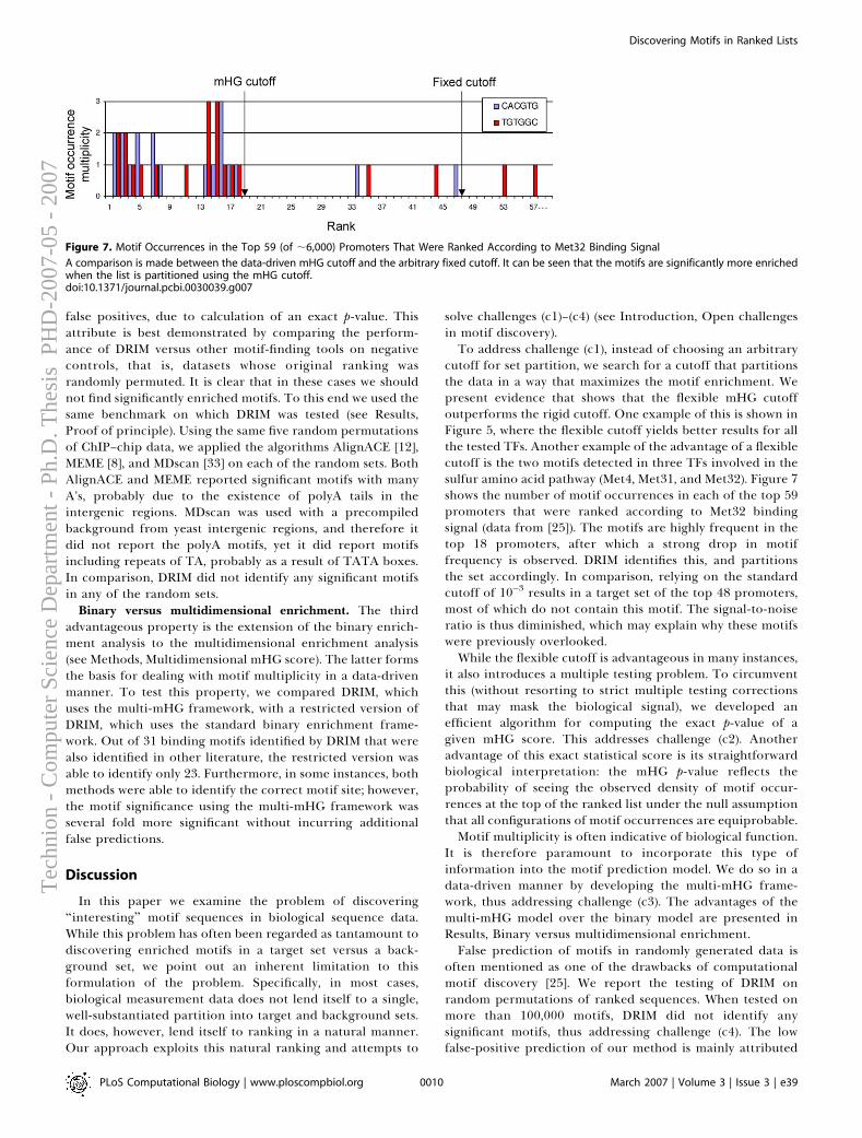
false positives, due to calculation of an exact p-value. Thisattribute is best demonstrated by comparing the perform-ance of DRIM versus other motif-finding tools on negativecontrols, that is, datasets whose original ranking wasrandomly permuted. It is clear that in these cases we shouldnot find significantly enriched motifs. To this end we used thesame benchmark on which DRIM was tested (see Results,Proof of principle). Using the same five random permutationsof ChIP–chip data, we applied the algorithms AlignACE [12],MEME [8], and MDscan [33] on each of the random sets. BothAlignACE and MEME reported significant motifs with manyA’s, probably due to the existence of polyA tails in theintergenic regions. MDscan was used with a precompiledbackground from yeast intergenic regions, and therefore itdid not report the polyA motifs, yet it did report motifsincluding repeats of TA, probably as a result of TATA boxes.In comparison, DRIM did not identify any significant motifsin any of the random sets.
Binary versus multidimensional enrichment. The thirdadvantageous property is the extension of the binary enrich-ment analysis to the multidimensional enrichment analysis(see Methods, Multidimensional mHG score). The latter formsthe basis for dealing with motif multiplicity in a data-drivenmanner. To test this property, we compared DRIM, whichuses the multi-mHG framework, with a restricted version ofDRIM, which uses the standard binary enrichment frame-work. Out of 31 binding motifs identified by DRIM that werealso identified in other literature, the restricted version wasable to identify only 23. Furthermore, in some instances, bothmethods were able to identify the correct motif site; however,the motif significance using the multi-mHG framework wasseveral fold more significant without incurring additionalfalse predictions.
Discussion
In this paper we examine the problem of discovering‘‘interesting’’ motif sequences in biological sequence data.While this problem has often been regarded as tantamount todiscovering enriched motifs in a target set versus a back-ground set, we point out an inherent limitation to thisformulation of the problem. Specifically, in most cases,biological measurement data does not lend itself to a single,well-substantiated partition into target and background sets.It does, however, lend itself to ranking in a natural manner.Our approach exploits this natural ranking and attempts to
solve challenges (c1)–(c4) (see Introduction, Open challengesin motif discovery).To address challenge (c1), instead of choosing an arbitrary
cutoff for set partition, we search for a cutoff that partitionsthe data in a way that maximizes the motif enrichment. Wepresent evidence that shows that the flexible mHG cutoffoutperforms the rigid cutoff. One example of this is shown inFigure 5, where the flexible cutoff yields better results for allthe tested TFs. Another example of the advantage of a flexiblecutoff is the two motifs detected in three TFs involved in thesulfur amino acid pathway (Met4, Met31, and Met32). Figure 7shows the number of motif occurrences in each of the top 59promoters that were ranked according to Met32 bindingsignal (data from [25]). The motifs are highly frequent in thetop 18 promoters, after which a strong drop in motiffrequency is observed. DRIM identifies this, and partitionsthe set accordingly. In comparison, relying on the standardcutoff of 10�3 results in a target set of the top 48 promoters,most of which do not contain this motif. The signal-to-noiseratio is thus diminished, which may explain why these motifswere previously overlooked.While the flexible cutoff is advantageous in many instances,
it also introduces a multiple testing problem. To circumventthis (without resorting to strict multiple testing correctionsthat may mask the biological signal), we developed anefficient algorithm for computing the exact p-value of agiven mHG score. This addresses challenge (c2). Anotheradvantage of this exact statistical score is its straightforwardbiological interpretation: the mHG p-value reflects theprobability of seeing the observed density of motif occur-rences at the top of the ranked list under the null assumptionthat all configurations of motif occurrences are equiprobable.Motif multiplicity is often indicative of biological function.
It is therefore paramount to incorporate this type ofinformation into the motif prediction model. We do so in adata-driven manner by developing the multi-mHG frame-work, thus addressing challenge (c3). The advantages of themulti-mHG model over the binary model are presented inResults, Binary versus multidimensional enrichment.False prediction of motifs in randomly generated data is
often mentioned as one of the drawbacks of computationalmotif discovery [25]. We report the testing of DRIM onrandom permutations of ranked sequences. When tested onmore than 100,000 motifs, DRIM did not identify anysignificant motifs, thus addressing challenge (c4). The lowfalse-positive prediction of our method is mainly attributed
Figure 7. Motif Occurrences in the Top 59 (of ;6,000) Promoters That Were Ranked According to Met32 Binding Signal
A comparison is made between the data-driven mHG cutoff and the arbitrary fixed cutoff. It can be seen that the motifs are significantly more enrichedwhen the list is partitioned using the mHG cutoff.doi:10.1371/journal.pcbi.0030039.g007
PLoS Computational Biology | www.ploscompbiol.org March 2007 | Volume 3 | Issue 3 | e390010
Discovering Motifs in Ranked ListsT
echn
ion
- C
ompu
ter
Scie
nce
Dep
artm
ent -
Ph.
D. T
hesi
s P
HD
-200
7-05
- 2
007
to the fact that it is based on rigorous statistics and relies onan exact p-value.
Another important issue that still requires consideration isthe characterization of the motif search space. In this studywe performed an exhaustive scanning of a restricted motifspace (containing ;105 motifs) followed by a heuristic searchfor larger motifs. However, the motif search space can befurther extended to include motifs that are longer, ‘‘fuzzier,’’or more complex. Additional considerations such as thedistance of the motif from the transcription start site may betaken into account as well as logical relations betweendifferent motifs (e.g., ‘‘OR,’’ ‘‘AND’’ operations). It is clearthat many of these features are required to correctly modelcomplex regulation patterns that are observed in highereukaryotes. Two inherent limitations need to be consideredwhen extending the search space: first, as the size of the motifsearch space increases, the problem of efficiently searchingthe defined space becomes more acute in terms of runningtime. Second, since the size of the search space is virtuallyendless, the problem of multiple testing rapidly erodes thesignal-to-noise ratio, requiring an appropriate refinement ofthe statistical models.
To test our method, we constructed a dataset containingChIP–chip experiments of 203 putative TFs in Saccharomycescerevisiae [25,28]. Surprisingly, we discovered a significantlength bias in roughly one-third of these experiments. Onepossible explanation for this phenomenon is nonspecificbinding between TFs and DNA, which causes longersequences to bind more TFs. This explanation is alsoconsistent with the ‘‘TF sliding hypothesis’’ [48]. Why onlysome TFs exhibit this length bias binding tendency remainsan open question. To avoid false positives due to thisphenomenon, we opted to filter out all ChIP–chip experi-ments that had significant length bias. Future work shouldaddress this point and focus on developing statistics that areinsensitive to this type of bias.
We analyzed the filtered dataset using DRIM and reportnovel putative TFBS motifs. Additional evidence thatindicates the newly discovered motifs are biologically func-tional was also presented. One interesting finding is that theAro80 motif we identified, which exists only in seven copiesthroughout the entire yeast genome, resides in Aro809s ownpromoter. This finding suggests that Aro80 regulates its owntranscription by binding to its own promoter. Additionally,three GATA binding sites that reside in the Aro80 promoteradjacent to the motif occurrence lead us to speculate thatAro809s putative self binding is inhibited by competingGATA binding factors (for details see Figure 4B).
Another interesting observation is the CA repeat motifs,which we identified in seven different yeast TFs as well as inhuman DNA methylation. This type of low complexity motifshave so far been mostly ignored or filtered out by othercomputational methods. By contrast there is no need toresort to this type of artificial filtering when using the mHGstatistics. Our findings in yeast suggest that for certain TFsthere is a significant correlation between a sequence’scapacity to bind a TF and the presence of a CA repeat inthe sequence. This supports a previous hypothesis that CArepeats alter the structure of DNA and thus contribute to TFbinding [34]. Our findings constitute concrete evidence ofthis phenomenon and suggest it may be more frequent thanpreviously appreciated.
We also applied DRIM to high-throughput measurements ofmethylated CpG islands [2] in human cancer cells, in order to tryto identify motifs that are enriched in hypermethylated regions.Interestingly, we identified GA and CA repeat elements as highlyenriched inmethylated CpG regions of four different cancer celllines. This is in agreement with previous studies of CpGmethylated regions in other cell lines [39,40]. It is interestingto ask whether these repeat elements play some active role inCpG methylation. In [40] the authors give statistical argumenta-tion against such a hypothesis. Instead, they hypothesize that CA(or TG) repeats are caused by an increased mutation rate ofmethylated CpGs that are deaminated into TpGs. Even if true,this still does not explain the enrichment of the GA repeats.Further experimental and bioinformatic interrogation of thispoint is therefore called upon.Overall, DRIM discovered ten novel motifs in methylated
CpG regions. Strikingly, nine of them are similar to DNAsequence elements that bind the Polycomb complex inDrosophila and/or human [41,42, 44]. The Polycomb complexis involved in epigenetic silencing via histone methylation.The suggested link between histone methylation and CpGmethylation is in agreement with recent work that demon-strated the EZH2 protein interacts with DNA methyltrans-ferases via the Polycomb complex [45]. We also note that theDNA sequence motifs of the two pathways were conserved inDrosophila and human, which is complementary to theobservation that the Polycomb proteins are evolutionarilyconserved [44,49]. Many of the motifs we found in the CpGmethylation data are similar across different types of cancercell lines. This may suggest that the CpG methylationmechanism is orchestrated by DNA binding factors that aresimilar in different types of cancer cell lines.Perhaps the most important conclusion that can be drawn
from this study is that looking at biological sequence data in aranked manner rather than using an arbitrary fixed cutoff topartition the data enables the detection of biological signalsthat are otherwise overlooked. This suggests that other motifdetection methods that rely on fixed cutoffs may benefit fromdynamic partitioning. While the effectiveness of our approachwas demonstrated on ChIP–chip and methylation data, it canalso be applied to a wide range of other data types such asexpression data or GO analysis. The DRIM application ispublicly available at http://bioinfo.cs.technion.ac.il/drim.
Materials and Methods
The minimum hypergeometric score. In this subsection weintroduce the basics of the mHG statistics, and demonstrate how it canbe applied in a straightforward manner to eliminate the need for anarbitrary choice of threshold. To explain the biological motivation ofmHG, consider the following scenario: suppose we have a set of promoterregions each associated with a measurement, e.g., a TF binding signal asmeasured by ChIP–chip [1]. We wish to determine whether a particularmotif specified in IUPAC notation, say CASGTGW, is likely to be a TFBSmotif. We rank the promoters according to their binding signals—strongbinding at the top of the list and the weak at the bottom (Figure 1i). Next,we generate a binary occurrence vector with one or zero entriesdependent on whether or not the respective promoter contains a copy ofthe motif (Figure 1ii). For simplicity we ignore cases where a promotercontains multiple copies of the motif (a refined model, which takes motifmultiplicity into account, will be discussed later). Motifs that yield binaryvectors with a high density of 19s at the top of the list are good candidatesfor being TFBS.
Let us assume for the moment that we know the correct physical-based cutoff on the TF binding signal. The data could then beseparated into ‘‘strong binding promoters’’ (i.e., the target set) and
PLoS Computational Biology | www.ploscompbiol.org March 2007 | Volume 3 | Issue 3 | e390011
Discovering Motifs in Ranked ListsT
echn
ion
- C
ompu
ter
Scie
nce
Dep
artm
ent -
Ph.
D. T
hesi
s P
HD
-200
7-05
- 2
007
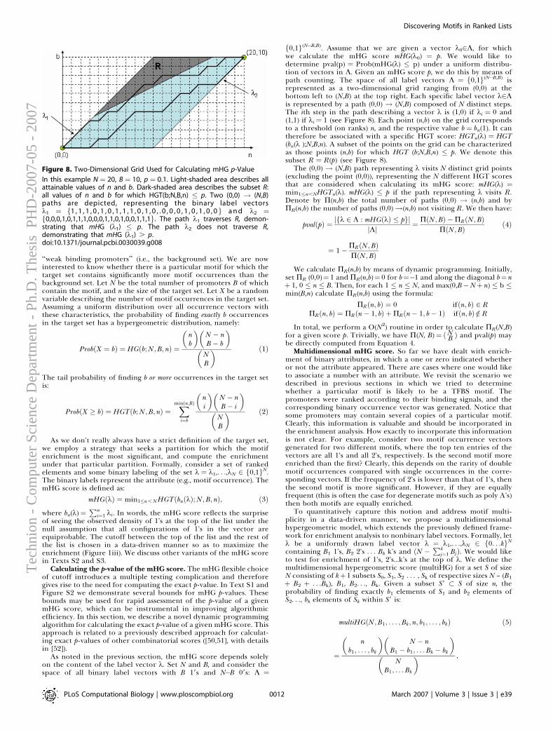
‘‘weak binding promoters’’ (i.e., the background set). We are nowinterested to know whether there is a particular motif for which thetarget set contains significantly more motif occurrences than thebackground set. Let N be the total number of promoters B of whichcontain the motif, and n the size of the target set. Let X be a randomvariable describing the number of motif occurrences in the target set.Assuming a uniform distribution over all occurrence vectors withthese characteristics, the probability of finding exactly b occurrencesin the target set has a hypergeometric distribution, namely:
ProbðX ¼ bÞ ¼ HGðb;N ;B; nÞ ¼
nb
� �N � nB� b
� �
NB
� � ð1Þ
The tail probability of finding b or more occurrences in the target setis:
ProbðX � bÞ ¼ HGTðb;N;B; nÞ ¼Xminðn;BÞ
i¼b
ni
� �N � nB� i
� �
NB
� � ð2Þ
As we don’t really always have a strict definition of the target set,we employ a strategy that seeks a partition for which the motifenrichment is the most significant, and compute the enrichmentunder that particular partition. Formally, consider a set of rankedelements and some binary labeling of the set k ¼ k1,. . .,kN 2 f0,1gN.The binary labels represent the attribute (e.g., motif occurrence). ThemHG score is defined as:
mHGðkÞ ¼ min1�n,NHGTðbnðkÞ;N;B; nÞ; ð3Þ
where bn(k)¼Pn
i¼1 ki. In words, the mHG score reflects the surpriseof seeing the observed density of 1’s at the top of the list under thenull assumption that all configurations of 1’s in the vector areequiprobable. The cutoff between the top of the list and the rest ofthe list is chosen in a data-driven manner so as to maximize theenrichment (Figure 1iii). We discuss other variants of the mHG scorein Texts S2 and S3.
Calculating the p-value of the mHG score. The mHG flexible choiceof cutoff introduces a multiple testing complication and thereforegives rise to the need for computing the exact p-value. In Text S1 andFigure S2 we demonstrate several bounds for mHG p-values. Thesebounds may be used for rapid assessment of the p-value of a givenmHG score, which can be instrumental in improving algorithmicefficiency. In this section, we describe a novel dynamic programmingalgorithm for calculating the exact p-value of a given mHG score. Thisapproach is related to a previously described approach for calculat-ing exact p-values of other combinatorial scores ([50,51], with detailsin [52]).
As noted in the previous section, the mHG score depends solelyon the content of the label vector k. Set N and B, and consider thespace of all binary label vectors with B 19s and N�B 09s: K ¼
f0,1g(N�B,B). Assume that we are given a vector k02K, for whichwe calculate the mHG score mHG(k0) ¼ p. We would like todetermine pval(p) ¼ Prob(mHG(k) � p) under a uniform distribu-tion of vectors in K. Given an mHG score p, we do this by means ofpath counting. The space of all label vectors K ¼ f0,1g(N�B,B) isrepresented as a two-dimensional grid ranging from (0,0) at thebottom left to (N,B) at the top right. Each specific label vector k2Kis represented by a path (0,0) ! (N,B) composed of N distinct steps.The ith step in the path describing a vector k is (1,0) if ki ¼ 0 and(1,1) if ki¼ 1 (see Figure 8). Each point (n,b) on the grid correspondsto a threshold (on ranks) n, and the respective value b ¼ bn(1). It cantherefore be associated with a specific HGT score: HGTn(k) ¼ HGT(bn(k );N,B,n). A subset of the points on the grid can be characterizedas those points (n,b) for which HGT (b;N,B,n) � p. We denote thissubset R ¼ R(p) (see Figure 8).
The (0,0) ! (N,B) path representing k visits N distinct grid points(excluding the point (0,0)), representing the N different HGT scoresthat are considered when calculating its mHG score: mHG(k) ¼min1�n,NHGTn(k). mHG(k) � p if the path representing k visits R.Denote by P(n,b) the total number of paths (0,0) ! (n,b) and byPR(n,b) the number of paths (0,0)!(n,b) not visiting R. We then have:
pvalðpÞ ¼ jfk 2 K : mHGðkÞ � pgjjKj ¼ PðN;BÞ �PRðN;BÞ
PðN;BÞ
¼ 1�PRðN;BÞPðN ;BÞ
ð4Þ
We calculate PR(n,b) by means of dynamic programming. Initially,set PR (0,0)¼1 and PR(n,b)¼0 for b¼�1 and along the diagonal b¼ nþ 1, 0 � n � B. Then, for each 1 � n � N, and max(0,B�Nþ n) � b �min(B,n) calculate PR(n,b) using the formula:
PRðn; bÞ ¼ 0 ifðn; bÞ 2 RPRðn; bÞ ¼ PRðn� 1; bÞ þPRðn� 1; b� 1Þ ifðn; bÞ =2 R
In total, we perform a O(N2) routine in order to calculate PR(N,B)for a given score p. Trivially, we have P(N, B)¼ ðNB Þ and pval(p) maybe directly computed from Equation 4.
Multidimensional mHG score. So far we have dealt with enrich-ment of binary attributes, in which a one or zero indicated whetheror not the attribute appeared. There are cases where one would liketo associate a number with an attribute. We revisit the scenario wedescribed in previous sections in which we tried to determinewhether a particular motif is likely to be a TFBS motif. Thepromoters were ranked according to their binding signals, and thecorresponding binary occurrence vector was generated. Notice thatsome promoters may contain several copies of a particular motif.Clearly, this information is valuable and should be incorporated inthe enrichment analysis. How exactly to incorporate this informationis not clear. For example, consider two motif occurrence vectorsgenerated for two different motifs, where the top ten entries of thevectors are all 1’s and all 2’s, respectively. Is the second motif moreenriched than the first? Clearly, this depends on the rarity of doublemotif occurrences compared with single occurrences in the corre-sponding vectors. If the frequency of 2’s is lower than that of 1’s, thenthe second motif is more significant. However, if they are equallyfrequent (this is often the case for degenerate motifs such as poly A’s)then both motifs are equally enriched.
To quantitatively capture this notion and address motif multi-plicity in a data-driven manner, we propose a multidimensionalhypergeometric model, which extends the previously defined frame-work for enrichment analysis to nonbinary label vectors. Formally, letk be a uniformly drawn label vector k ¼ k1,. . .,kN 2 f0. . .kgNcontaining B1 1’s, B2 2’s . . . Bk k’s and ðN �
Pkj¼1 BjÞ. We would like
to test for enrichment of 1’s, 2’s...k’s at the top of k. We define themultidimensional hypergeometric score (multiHG) for a set S of sizeN consisting of kþ1 subsets S0, S1, S2 . . . , Sk of respective sizes N – (B1þ B2 þ . . .Bk), B1, B2. . ., Bk. Given a subset S9 � S of size n, theprobability of finding exactly b1 elements of S1 and b2 elements ofS2. . ., bk elements of Sk within S9 is:
multiHGðN ;B1; . . . ;Bk; n; b1; . . . ; bkÞ
¼
nb1; . . . ; bk
� �N � n
B1 � b1; . . .Bk � bk
� �
NB1; . . .Bk
� � ;
ð5Þ
Figure 8. Two-Dimensional Grid Used for Calculating mHG p-Value
In this example N ¼ 20, B ¼ 10, p ¼ 0.1. Light-shaded area describes allattainable values of n and b. Dark-shaded area describes the subset R:all values of n and b for which HGT(b;N,B,n) � p. Two (0,0) ! (N,B)paths are depicted, representing the binary label vectorsk1 ¼ f1 , 1 , 1 , 0 , 1 , 0 , 1 , 1 , 1 , 0 , 1 , 0 , . 0 , 0 , 0 , 1 , 0 , 1 , 0 , 0g a n d k2 ¼f0,0,0,1,0,1,1,1,0,0,0,1,1,0,1,0,0,1,1,1g. The path k1 traverses R, demon-strating that mHG (k1) � p. The path k2 does not traverse R,demonstrating that mHG (k1) . p.doi:10.1371/journal.pcbi.0030039.g008
PLoS Computational Biology | www.ploscompbiol.org March 2007 | Volume 3 | Issue 3 | e390012
Discovering Motifs in Ranked ListsT
echn
ion
- C
ompu
ter
Scie
nce
Dep
artm
ent -
Ph.
D. T
hesi
s P
HD
-200
7-05
- 2
007
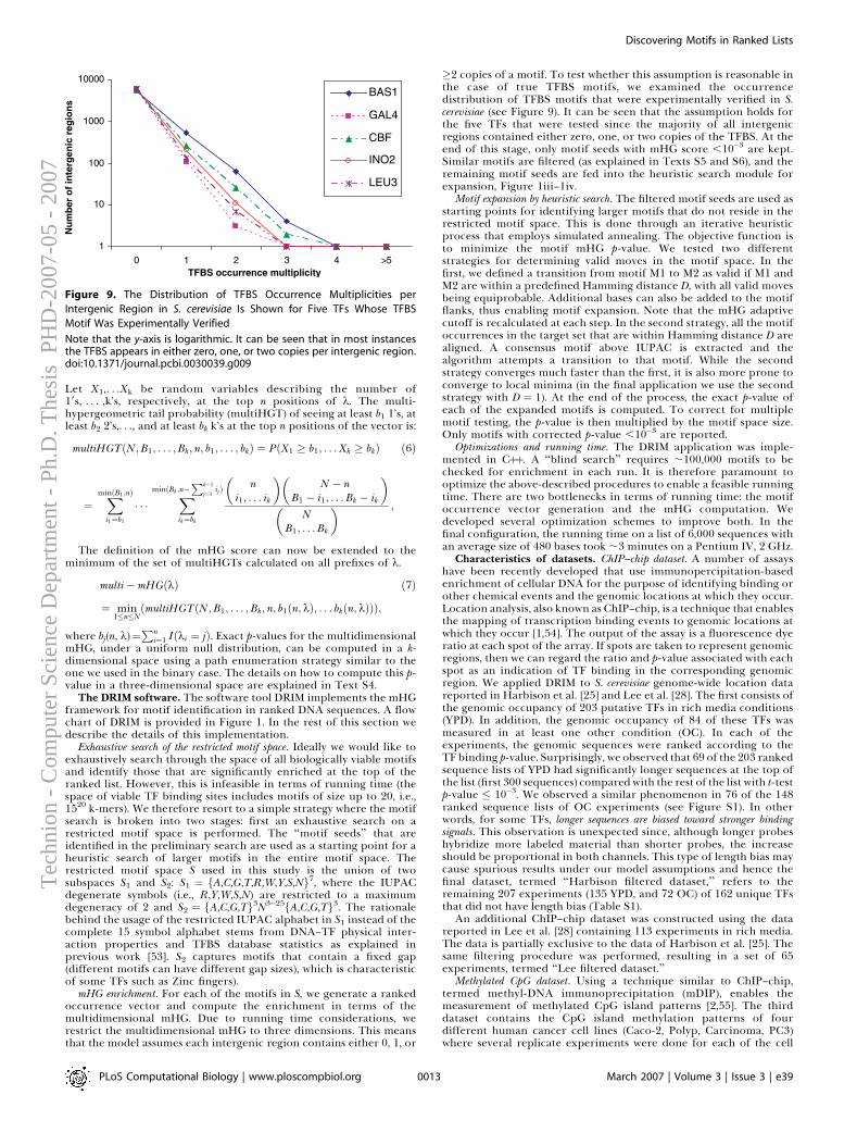
Let X1,. . .Xk be random variables describing the number of19s, . . . ,k’s, respectively, at the top n positions of k. The multi-hypergeometric tail probability (multiHGT) of seeing at least b1 1’s, atleast b2 2’s,. . ., and at least bk k’s at the top n positions of the vector is:
multiHGTðN ;B1; . . . ;Bk; n; b1; . . . ; bkÞ ¼ PðX1 � b1; . . .Xk � bkÞ
¼XminðB1 ;nÞ
i1¼b1� � �
XminðBk ;n�Pk�1
j¼1 ijÞ
ik¼bk
ni1; . . . ik
� �N � n
B1 � i1; . . .Bk � ik
� �
NB1; . . .Bk
� � ;
ð6Þ
The definition of the mHG score can now be extended to theminimum of the set of multiHGTs calculated on all prefixes of k.
multi� mHGðkÞ
¼ min1�n�N
ðmultiHGTðN;B1; . . . ;Bk; n; b1ðn;kÞ; . . . bkðn; kÞÞÞ;
ð7Þ
where bj(n, k)¼Pn
i¼1 Iðki ¼ jÞ. Exact p-values for the multidimensionalmHG, under a uniform null distribution, can be computed in a k-dimensional space using a path enumeration strategy similar to theone we used in the binary case. The details on how to compute this p-value in a three-dimensional space are explained in Text S4.
The DRIM software. The software tool DRIM implements the mHGframework for motif identification in ranked DNA sequences. A flowchart of DRIM is provided in Figure 1. In the rest of this section wedescribe the details of this implementation.
Exhaustive search of the restricted motif space. Ideally we would like toexhaustively search through the space of all biologically viable motifsand identify those that are significantly enriched at the top of theranked list. However, this is infeasible in terms of running time (thespace of viable TF binding sites includes motifs of size up to 20, i.e.,1520 k-mers). We therefore resort to a simple strategy where the motifsearch is broken into two stages: first an exhaustive search on arestricted motif space is performed. The ‘‘motif seeds’’ that areidentified in the preliminary search are used as a starting point for aheuristic search of larger motifs in the entire motif space. Therestricted motif space S used in this study is the union of twosubspaces S1 and S2: S1 ¼ fA,C,G,T,R,W,Y,S,Ng7, where the IUPACdegenerate symbols (i.e., R,Y,W,S,N) are restricted to a maximumdegeneracy of 2 and S2 ¼ fA,C,G,Tg3N3�25fA,C,G,Tg3. The rationalebehind the usage of the restricted IUPAC alphabet in S1 instead of thecomplete 15 symbol alphabet stems from DNA–TF physical inter-action properties and TFBS database statistics as explained inprevious work [53]. S2 captures motifs that contain a fixed gap(different motifs can have different gap sizes), which is characteristicof some TFs such as Zinc fingers).
mHG enrichment. For each of the motifs in S, we generate a rankedoccurrence vector and compute the enrichment in terms of themultidimensional mHG. Due to running time considerations, werestrict the multidimensional mHG to three dimensions. This meansthat the model assumes each intergenic region contains either 0, 1, or
�2 copies of a motif. To test whether this assumption is reasonable inthe case of true TFBS motifs, we examined the occurrencedistribution of TFBS motifs that were experimentally verified in S.cerevisiae (see Figure 9). It can be seen that the assumption holds forthe five TFs that were tested since the majority of all intergenicregions contained either zero, one, or two copies of the TFBS. At theend of this stage, only motif seeds with mHG score ,10�3 are kept.Similar motifs are filtered (as explained in Texts S5 and S6), and theremaining motif seeds are fed into the heuristic search module forexpansion, Figure 1iii–1iv.
Motif expansion by heuristic search. The filtered motif seeds are used asstarting points for identifying larger motifs that do not reside in therestricted motif space. This is done through an iterative heuristicprocess that employs simulated annealing. The objective function isto minimize the motif mHG p-value. We tested two differentstrategies for determining valid moves in the motif space. In thefirst, we defined a transition from motif M1 to M2 as valid if M1 andM2 are within a predefined Hamming distance D, with all valid movesbeing equiprobable. Additional bases can also be added to the motifflanks, thus enabling motif expansion. Note that the mHG adaptivecutoff is recalculated at each step. In the second strategy, all the motifoccurrences in the target set that are within Hamming distance D arealigned. A consensus motif above IUPAC is extracted and thealgorithm attempts a transition to that motif. While the secondstrategy converges much faster than the first, it is also more prone toconverge to local minima (in the final application we use the secondstrategy with D ¼ 1). At the end of the process, the exact p-value ofeach of the expanded motifs is computed. To correct for multiplemotif testing, the p-value is then multiplied by the motif space size.Only motifs with corrected p-value ,10�3 are reported.
Optimizations and running time. The DRIM application was imple-mented in Cþþ. A ‘‘blind search’’ requires ;100,000 motifs to bechecked for enrichment in each run. It is therefore paramount tooptimize the above-described procedures to enable a feasible runningtime. There are two bottlenecks in terms of running time: the motifoccurrence vector generation and the mHG computation. Wedeveloped several optimization schemes to improve both. In thefinal configuration, the running time on a list of 6,000 sequences withan average size of 480 bases took ;3 minutes on a Pentium IV, 2 GHz.
Characteristics of datasets. ChIP–chip dataset. A number of assayshave been recently developed that use immunopercipitation-basedenrichment of cellular DNA for the purpose of identifying binding orother chemical events and the genomic locations at which they occur.Location analysis, also known as ChIP–chip, is a technique that enablesthe mapping of transcription binding events to genomic locations atwhich they occur [1,54]. The output of the assay is a fluorescence dyeratio at each spot of the array. If spots are taken to represent genomicregions, then we can regard the ratio and p-value associated with eachspot as an indication of TF binding in the corresponding genomicregion. We applied DRIM to S. cerevisiae genome-wide location datareported in Harbison et al. [25] and Lee et al. [28]. The first consists ofthe genomic occupancy of 203 putative TFs in rich media conditions(YPD). In addition, the genomic occupancy of 84 of these TFs wasmeasured in at least one other condition (OC). In each of theexperiments, the genomic sequences were ranked according to theTF binding p-value. Surprisingly, we observed that 69 of the 203 rankedsequence lists of YPD had significantly longer sequences at the top ofthe list (first 300 sequences) comparedwith the rest of the list with t-testp-value � 10�3. We observed a similar phenomenon in 76 of the 148ranked sequence lists of OC experiments (see Figure S1). In otherwords, for some TFs, longer sequences are biased toward stronger bindingsignals. This observation is unexpected since, although longer probeshybridize more labeled material than shorter probes, the increaseshould be proportional in both channels. This type of length bias maycause spurious results under our model assumptions and hence thefinal dataset, termed ‘‘Harbison filtered dataset,’’ refers to theremaining 207 experiments (135 YPD, and 72 OC) of 162 unique TFsthat did not have length bias (Table S1).
An additional ChIP–chip dataset was constructed using the datareported in Lee et al. [28] containing 113 experiments in rich media.The data is partially exclusive to the data of Harbison et al. [25]. Thesame filtering procedure was performed, resulting in a set of 65experiments, termed ‘‘Lee filtered dataset.’’
Methylated CpG dataset. Using a technique similar to ChIP–chip,termed methyl-DNA immunoprecipitation (mDIP), enables themeasurement of methylated CpG island patterns [2,55]. The thirddataset contains the CpG island methylation patterns of fourdifferent human cancer cell lines (Caco-2, Polyp, Carcinoma, PC3)where several replicate experiments were done for each of the cell
Figure 9. The Distribution of TFBS Occurrence Multiplicities per
Intergenic Region in S. cerevisiae Is Shown for Five TFs Whose TFBS
Motif Was Experimentally Verified
Note that the y-axis is logarithmic. It can be seen that in most instancesthe TFBS appears in either zero, one, or two copies per intergenic region.doi:10.1371/journal.pcbi.0030039.g009
PLoS Computational Biology | www.ploscompbiol.org March 2007 | Volume 3 | Issue 3 | e390013
Discovering Motifs in Ranked ListsT
echn
ion
- C
ompu
ter
Scie
nce
Dep
artm
ent -
Ph.
D. T
hesi
s P
HD
-200
7-05
- 2
007
lines. In each of these experiments, the CpG methylation signal wasmeasured in ;13,000 gene promoters as reported in [2].
Supporting Information
Figure S1. Observed versus Expected Length Bias
For each of the 148 OC ChIP–chip experiments reported in [25], weranked the yeast intergenic sequences according to their bindingsignal. The lengths of the top 300 sequences in each experiment werecompared with the lengths of the rest of the sequences using astudent t-test. The x-axis is the t-test p-value and y(x) is the number ofTF experiments with p � x. The blue line is the observed cumulativedistribution of the t-test p-values in the 148 experiments. The red lineis the expected cumulative distribution of t-test p-values in randomlypermuted sequence rankings. It can be seen that more than half ofthe ChIP–chip experiments have a statistically significant differencebetween the lengths of sequences that bind the TF the strongestcompared with the lengths of the rest of the sequences.
Found at doi:10.1371/journal.pcbi.0030039.sg001 (21 KB PNG).
Figure S2. Comparison of p-Value Bounds, Exact p-Value Calculation,and Observed Frequencies of mHG Scores for Two Synthetic Cases:(A) N¼ 600, B¼ 300; (B) N ¼ 330, B ¼ 30
In each case the following values were generated for several differentmHG scores: lower bound (p), trivial upper bound (Np), tighter upperbound (Bp), exact p-value calculation (pVal), and observed p-valuesover 10,000 random instances (sim). Note the improvement of thetighter upper bound (Bp) when N � B.
Found at doi:10.1371/journal.pcbi.0030039.sg002 (13 KB PNG).
Figure S3. Comparison of mHG Score and p-Value Distributions forMotifs inRandomlyRankedSequenceswithThose ofTrueTFBSMotifsin Ranked Lists Derived from the Corresponding ChIP–chip Assays
;100,000 motifs were scanned in 400 randomly ranked genomicsequences, and their corresponding corrected p-value (A) andmHG score(B) were recorded. The corrected p-values involve two levels of multipletest corrections: correction on the number motifs that were tested; andcorrection for the multiple cutoffs that are tested as part of the mHGoptimization process. None of the testedmotifs had a corrected p-value,10�3. DRIM was applied on the ChIP–chip data of five TFs and the mHGscores, and corrected p-values of the true TFBS motifs (as previouslydeterminedexperimentally)were recorded. In all instances, the trueTFBSmotifs were predictedwith p-values thatwere several orders ofmagnitudemore significant than the best random set motif p-value.Found at doi:10.1371/journal.pcbi.0030039.sg003 (81 KB JPG).
Figure S4. Compatibility between the BSAro80 Motif Identified byDRIM and Previously Reported Mutagenesis Studies [32]
The Aro9 promoter region from base�169 to�133 as well as six othercopies containing mutations and deletions are shown. These regionswere used to construct hybrid promoters and measure the expressionof a reporter gene, which is dependent on the binding of Aro80 to thepromoter [32]. The two partially overlapping copies of BSAro80 thatreside in the Aro9 promoter and an additional sequence element thatis similar to the canonic BSAro80 (two different bases) are marked withgreen and blue arrows, respectively. It can be seen that the expressionvalues are highly compatible with the number of intact BSAro80copies, i.e., more intact copies yield higher expression.
Found at doi:10.1371/journal.pcbi.0030039.sg004 (11 KB PNG).
Figure S5. Met4-Met28-CBF and Met4-Met28-Met31/32 ComplexesBinding to DNA
(A) Schematic representation of Met4-Met28-CBF and Met4-Met28-Met31/32 complexes [37,38].(B) A hypothetical Met4-Met28-CBF-Met31/32 complex. Immunopre-cipitation of any of the TFs in the complex will precipitate the sameset of sequences, which explains why DRIM identifies the same twomotifs for all TFs in the complex.
Found at doi:10.1371/journal.pcbi.0030039.sg005 (67 KB PNG).
Figure S6. Comparison of the mHG and HG Methods on Simulationsof Motif Occurrence Vectors
The vectors were generated according to a rank-dependent distribu-
tion (see the section, Comparing mHG and HG on simulated motifoccurrences) with 18 different parameter combinations (a ¼ 10, 50,100; b¼ 0.01, 0.05, 0.1; u¼ 0.01, 0.1). The�log fraction between mHGand HG p-values in cases where the p-value of one of the methods wassmaller than 10�3 are shown.
Found at doi:10.1371/journal.pcbi.0030039.sg006 (117 KB JPG).
Table S1. List of TFs in the Harbison Filtered Dataset
Found at doi:10.1371/journal.pcbi.0030039.st001 (27 KB XLS).
Table S2. Motif Predictions of DRIM on the Harbison FilteredDataset
Found at doi:10.1371/journal.pcbi.0030039.st002 (245 KB XLS).
Table S3. Comparison between the Predictions of DRIM and ThoseReported in [25]
Found at doi:10.1371/journal.pcbi.0030039.st003 (18 KB XLS).
Table S4. Comparison between mHG Flexible Cutoffs and 10�3 FixedCutoffs in Yeast ChIP–chip Data
Found at doi:10.1371/journal.pcbi.0030039.st004 (15 KB XLS).
Table S5. Gene Accession Numbers
The National Center for Biotechnology Information (NCBI) (http://www.ncbi.nlm.nih.gov) accession numbers for the genes discussed inthe paper.
Found at doi:10.1371/journal.pcbi.0030039.st005 (18 KB XLS).
Text S1. Bounds for the mHG p-Value
Found at doi:10.1371/journal.pcbi.0030039.sd001 (137 KB DOC).
Text S2. Partition-Limited mHG Score
Found at doi:10.1371/journal.pcbi.0030039.sd002 (24 KB DOC).
Text S3. mHG and Expression
Found at doi:10.1371/journal.pcbi.0030039.sd003 (24 KB DOC).
Text S4. p-Value of the Three-Dimensional mHG Score
Found at doi:10.1371/journal.pcbi.0030039.sd004 (47 KB DOC).
Text S5. Motif Similarity
Found at doi:10.1371/journal.pcbi.0030039.sd005 (38 KB DOC).
Text S6. Filtering Similar Motifs
Found at doi:10.1371/journal.pcbi.0030039.sd006 (24 KB DOC).
Text S7. Comparing mHG and HG on Simulated Motif Occurrences
Found at doi:10.1371/journal.pcbi.0030039.sd007 (21 KB DOC).
Accession Numbers
Accession numbers for the genes discussed in the paper are given inTable S5.
Acknowledgments
We thank Mark Silberstein of the Technion for assistance withconnecting the DRIM application to the Condor computer grid, AmirBen-Dor of Agilent Laboratories, and Nir Friedman of the HebrewUniversity for useful discussions and ideas related to characterizingthe distribution of mHG; Naama Hazan and Gal Shaul for testingDRIM on the CREB data; and the authors also thank Itamar Simon ofthe Hebrew University for access to the CpG methylation data.
Author contributions. EE, DL, and ZY designed the study. EE, DL,SY, and ZY developed the statistics and algorithms. EE and SYdeveloped the software and performed the data analysis. EE, DL, andZY wrote the paper.
Funding. EE was supported by the Gutwirth fellowship. DL wassupported by an Agilent PhD Fellowship. EE and ZY were partiallysupported by a European Union FP6 grant, under the framework ofthe MultiKnowledge Project.
Competing interests. The authors have declared that no competinginterests exist.
PLoS Computational Biology | www.ploscompbiol.org March 2007 | Volume 3 | Issue 3 | e390014
Discovering Motifs in Ranked ListsT
echn
ion
- C
ompu
ter
Scie
nce
Dep
artm
ent -
Ph.
D. T
hesi
s P
HD
-200
7-05
- 2
007
References1. Ren B, Robert F, Wyrick J, Aparicio O, Jennings E, et al. (2000) Genome-
wide location and function of DNA binding proteins. Science 290: 2306–2309.
2. Keshet I, Schlesinger Y, Farkash S, Rand E, Hecht M, et al. (2006) Evidencefor an instructive mechanism of de novo methylation in cancer cells. NatGenet 38: 149–153.
3. Bussemaker H, Li H, Siggia E (2001) Regulatory element detection usingcorrelation with expression. Nat Genet 27: 167–71.
4. Sinha S, Tompa M (2002) Discovery of novel transcription factor bindingsites by statistical overrepresentation. Nucleic Acids Res 30: 5549–5560.
5. Sinha S, Tompa M (2003) Ymf: A program for discovery of noveltranscription factor binding sites by statistical overrepresentation. NucleicAcids Res 31: 3586–3588.
6. Workman C, Stromo G (2000) ANN-SPEC: A method for discoveringtranscription factor binding sites with improved specificity. Pac SympBiocomput 5: 464–475.
7. Barash Y, Bejerano G, Friedman N (2001) A simple hyper-geometricapproach for discovering putative transcription factor binding sites. In:Gascuel O, Moret BME, editors. Proceedings of the First InternationalWorkshop (WABI); 28–31 August 2001; Aarhus, Denmark. Algorithms inBioinformatics. Berlin: Springer. Lecture Notes Comp Sci 2149: 278–293.
8. Bailey T, Elkan C (1994) Fitting a mixture model by expectationmaximization to discover motifs in biopolymers. ISMB 28–36.
9. Liu X, Brutlag D, Liu J (2001) . Liu X, Brutlag D, Liu J (2001) Bioprospector:Discovering conserved DNA motifs in upstream regulatory regions of co-expressed genes. Pac Symp Biocomput 127–138.
10. Hong P, Liu XS, Zhou Q, Lu X, Liu JS, et al. (2005) A boosting approach formotif modeling using ChIP–chip data. Bioinformatics 21: 2636–2643.
11. Smith AD, Sumazin P, Das D, Zhang MQ (2005) Mining ChIP–chip data fortranscription factor and cofactor binding sites. Bioinformatics 21: 408–412.
12. Roth F, Hughes J, Estep P, Church G (1998) Finding DNA regulatory motifswithin unaligned noncoding sequences clustered by whole-genome mRNAquantitation. Nat Biotechnol 16: 939–945.
13. Ben-Gal I, Shani A, Gohr A, Grau J, Arviv S, et al. (2005) Identification oftranscription factor binding sites with variable-order Bayesian networks.Bioinformatics 21: 2657–2666.
14. Tompa M, Li N, Bailey T, Church G, Moor BD, et al. (2005) Assessingcomputational tools for the discovery of transcription factor binding sites.Nat Biotechnol 23: 137–144.
15. MacIsaac K, Fraenkel E (2006) Practical strategies for discoveringregulatory DNA sequence motifs. PLoS Comput Biol 2: 201–210.
16. Hu J, Li B, Kihara D (2005) Limitations and potentials of current motifdiscovery algorithms. Nucleic Acids Res 33: 4899–4913.
17. Bulyk M (2003) Computational prediction of transcription-factor bindingsite locations. Genome Biol 5: 201.
18. Friberg M, von Rohr P, Gonnet G (2005) Scoring functions for tran-scription factor binding site prediction. BMC Bioinformatics 6: 84.
19. Das D, Nahle Z, Zhang MQ (2006) Adaptively inferring human transcrip-tional subnetworks. Mol Sys Biol 2: 29.
20. Sinha S, Liang Y, Siggia E (2006) Stubb: A program for discovery andanalysis of cis-regulatory modules. Nucleic Acids Res 34: 555–559.
21. Thompson W, Rouchka E, Lawrence CE (2003) Gibbs recursive sampler:Finding transcription factor binding sites. Nucleic Acids Res 31: 3580–3585.
22. Hallikas O, Palin K, Sinjushina N, Rautiainen R, Partanen J, et al. (2006)Genome-wide prediction of mammalian enhancers based on analysis oftranscription-factor binding affinity. Cell 124: 47–59.
23. Gupta M, Liu J (2005) De novo cis-regulatory module elicitation foreukaryotic genomes. Proc Natl Acad Sci U S A 102: 7079–7084.
24. Jensen L, Knudsen S (2000) Automatic discovery of regulatory patterns inpromoter regions based on whole cell expression data and functionalannotation. Bioinformatics 16: 326–333.
25. Harbison C, Gordon D, Lee T, Rinaldi N, Macisaac K, et al. (2004)Transcriptional regulatory code of a eukaryotic genome. Nature 431: 99–104.
26. Ben-Zaken Zilberstein C, Eskin E, Yakhini Z (2004) Using expression data todiscover RNA and DNA regulatory sequence motifs. Proceedings of theFirst Annual RECOMB Satellite Workshop on Regulatory Genomics; 26–27March 2004; San Diego, California, United States. Berlin: Springer-Verlag.pp. 65–78.
27. Zhu Z, Pilpel Y, Church G (2002) Computational identification oftranscription factor binding sites via a transcription-factor-centricclustering (tfcc) algorithm. J Mol Biol 318: 71–81.
28. Lee T, Rinaldi N, Robert F, Odom D, Bar-Joseph Z, et al. (2002)Transcriptional regulatory networks in Saccharomyces cerecisiae. Science298: 799–804.
29. MacIsaac K, Wang T, Gordon B, Gifford D, Stromo G, et al. (2006) Animproved map of conserved regulatory sites for Saccharomyces cerevisiae.BMC Bioinformatics 7.
30. Vuralhan Z, Morais M, Tai S, Piper M, Pronk J (2003) Identification and
characterization of phenylpyruvate decarboxylase genes in Saccharomycescerevisiae. Appl Environ Microbiol 69: 4534–4541.
31. Etschmann M, Bluemke W, Sell D, Schrader J (2002) Biotechnologicalproduction of 2-phenylethanol. Appl Microbiol Biotechnol 59: 1–8.
32. Iraqui I, Vissers S, Andre B, Urrestarazu A (1999) Transcriptional inductionby aromatic amino acids in Saccharomyces cerevisiae. Mol Cell Biol 19: 3360–3371.
33. Liu X, Brutlag D, Liu J (2002) An algorithm for finding protein–DNAbinding sites with applications to chromatin-immunoprecipitation micro-array experiments. Nat Biotechnol 20: 835–839.
34. Nussinov R (1986) Some guidelines for identification of recognitionsequences: Regulatory sequences frequently contain (t)gtg/cac(a), tga/tcaand (t)ctc/gag(a). Biochim Biophys Acta 866: 93–108.
35. Anagnou N, Moulton A, Keller G, Karlsson S, Papayannopoulou T, et al.(1985) Cis-acting sequences that affect the expression of the human fetalgamma-globin genes. Prog Clin Biol Res 191: 163–182.
36. Anderson S, Steber C, Esposito R, Coleman J (1995) Ume6, a negativeregulator of meiosis in Saccharomyces cerevisiae, contains a c-terminalZn2Cys6 binuclear cluster that binds the URS1 DNA sequence in a zinc-dependent manner. Protein Science 4: 1832–1843.
37. Blaiseau P, Thomas D (1998) Multiple transcriptional activation complexestether the yeast activator Met4 to DNA. EMBO J 17: 6327–6336.
38. Blaiseau P, Isnard A, Surdin-Kerjan Y, Thomas D (1997) Met31p andMet32p, two related zinc finger proteins, are involved in transcriptionalregulation of yeast sulfur amino acid metabolism. Mol Cell Biol 17: 3640–3648.
39. Feltus FA, Lee EK, Costello JF, Plass C, Vertino PM (2003) Predictingaberrant CpG islands methylation. Proc Natl Acad Sci U S A 100: 12253–12258.
40. Bock1 C, Paulsen M, Tierling S, Mikeska T, Lengauer T, et al. (2006) CpGisland methylation in human lymphocytes is highly correlated with DNAsequence, repeats, and predicted DNA structure. PLoS Genetics 2: 243–252.
41. Ringrose L, Rehmsmeier M, Dura J, Paro R (2003) Genome-wide predictionof polycomb/trithorax response elements in Drosophila melanogaster. Dev Cell5: 759–771.
42. Lee T, Jenner R, Boyer L, Guenther M, Levine S, et al. (2006) Control ofdevelopmental regulators by polycomb in human embryonic stem cells.Cell 125: 301–313.
43. Strutt H, Cavalli G, Paro1 R (1997) Co-localization of polycomb protein andGAGA factor on regulatory elements responsible for the maintenance ofhomeotic gene expression. EMBO J 16: 3621–3632.
44. Bracken A, Dietrich N, Pasini D, Hansen K, Helin K (2006) Genome-widemapping of polycomb target genes unravels their roles in cell fatetransitions. Genes Dev 20: 1123–1136.
45. Vire E, Brenner C, Deplus R, Blanchon L, Fraga M, et al. (2006) Thepolycomb group protein EZH2 directly controls DNA methylation. Nature439: 871–874.
46. Odom D, Zizlsperger N, Gordon D, Bell G, Rinaldi N, et al. (2004) Controlof pancreas and liver gene expression by hnf transcription factors. Science303: 1378–1381.
47. Zhang X, Odom D, Koo S, Conkright M, Canettieri G, et al. (2005) Genome-wide analysis of camp-response element binding protein occupancy,phosphorylation, and target gene activation in human tissues. Proc NatlAcad Sci U S A 102: 4459–4464.
48. Deremble C, Lavery R (2005) Macromolecular recognition. Curr OpinStruct Biol 15: 171–175.
49. Levine S, Weiss A, Erdjument-Bromage H, Shao Z, Tempst P, et al. (2002)The core of the polycomb repressive complex is compositionally andfunctionally conserved in flies and humans. Mol Cell Biol 22: 6070–6080.
50. Ben-Dor A, Bruhn L, Friedman N, Nachman I, Schummer M, et al. (2000)Tissue classification with gene expression profiles. J Comput Biol 7: 559–583.
51. Bittner M, Meltzer P, Chen Y, Jiang Y, Seftor E, et al. (2000) Molecularclassification of cutaneous malignant melanoma by gene expressionprofiling. Nature 406: 536–540.
52. Ben-Dor A, Friedman N, Yakhini Z (2000) Scoring genes for relevance.Technical Report 2000–38. Jerusalem: Hebrew University School ofComputer Science and Engineering. Available: http://www.agilent.com/labs/research/papers/AGL-2000–13.pdf. Accessed 12 February 2007.
53. Sinha S, Tompa M (2000) A statistical method for finding transcriptionfactor binding sites. ISMB 8: 344–354.
54. Buck M, Lieb JD (2003) ChIP–chip: Considerations for design, analysis, andapplication of genome-wide chromatin immunoprecipitation experiments.Genomics 83: 349–360.
55. Shi H, Maier S, Nimmrich I, Yan P, Caldwell C, et al. (2003) Oligonucleo-tide-based microarray for DNA methylation analysis: Principles andapplications. J Cell Biochem 88: 138–143.
56. Gorodkin J, Heyer LJ, Brunak S, Stormo GD (1997) Displaying theinformation contents of structural RNA alignments: The structure logos.Comp Appl Biosci 13: 583–586.
PLoS Computational Biology | www.ploscompbiol.org March 2007 | Volume 3 | Issue 3 | e390015
Discovering Motifs in Ranked ListsT
echn
ion
- C
ompu
ter
Scie
nce
Dep
artm
ent -
Ph.
D. T
hesi
s P
HD
-200
7-05
- 2
007