Efficient Calculation of Interval Scores for DNA CopyNumber Data Analysis

Doron Lipson1, Yonatan Aumann2, Amir Ben-Dor3, Nathan Linial4, and Zohar Yakhini1,3

1 Computer Science Dept., Technion, Haifa2 Computer Science Dept., Bar-Ilan University, Ramat Gan

3 Agilent Laboratories4 Computer Science Dept., Hebrew University of Jerusalem

AbstractBackground. DNA amplifications and deletions characterize cancer genome and are of-

ten related to disease evolution. Microarray based techniques for measuring these DNAcopy-number changes use fluorescence ratios at arrayed DNA elements (BACs, cDNA oroligonucleotides) to provide signals at high resolution, in terms of genomic locations. Thesedata are then further analyzed to map aberrations and boundaries and identify biologicallysignificant structures.Methods. We develop a statistical framework that enables the casting of several DNA copynumber data analysis questions as optimization problems over real valued vectors of sig-nals. The simplest form of the optimization problem seeks to maximize ϕ(I) =

∑vi/√|I|

over all subintervals I in the input vector. We present and prove a linear time approximationscheme for this problem. Namely, a process with time complexity O

(nε−2

)that outputs an

interval for which ϕ(I) is at least Opt/α(ε), where Opt is the actual optimum and α(ε)→ 1as ε → 0. We further develop practical implementations that improve the performance ofthe naive quadratic approach by orders of magnitude. We discuss properties of optimal in-tervals and how they apply to the algorithm performance.Examples. We benchmark our algorithms on synthetic as well as publicly available DNAcopy number data. We demonstrate the use of these methods for identifying aberrationsin single samples as well as common alterations in fixed sets and subsets of breast cancersamples.

1 Introduction

Alterations in DNA copy number are characteristic of many cancer types and are thoughtto drive some cancer pathogenesis processes. These alterations include large chromosomalgains and losses as well as smaller scale amplifications and deletions. Because of their rolein cancer development, regions of chromosomal instability are useful for elucidating othercomponents of the process. For example, since genomic instability can trigger the overexpression or activation of oncogenes and the silencing of tumor suppressors, mappingregions of common genomic aberrations has been used to discover cancer related genes.Understanding genome aberrations is important for both the basic understanding of cancerand for diagnosis and clinical practice.

Alterations in DNA copy number have been initially measured using local fluores-cence in situ hybridization-based techniques. These evolved to a genome wide technique

called Comparative Genomic Hybridization (CGH, see [11]), now commonly used for theidentification of chromosomal alterations in cancer [13, 1]. In this genome-wide cytoge-netic method differentially labeled tumor and normal DNA are co-hybridized to normalmetaphases. Ratios between the two labels allow the detection of chromosomal amplifi-cations and deletions of regions that may harbor oncogenes and tumor suppressor genes.Classical CGH has, however, a limited resolution (10-20 Mbp). With such low resolutionit is impossible to predict the borders of the chromosomal changes or to identify changesin copy numbers of single genes and small genomic regions. In a more advanced methodtermed array CGH (aCGH), tumor and normal DNA are co-hybridized to a microarray ofthousands of genomic clones of BAC, cDNA or oligonucleotide probes [17, 10, 15, 19, 4,3]. The use of aCGH allows the determination of changes in DNA copy number of rel-atively small chromosomal regions. Using oligonucleotides arrays the resolution can, intheory, be finer than single genes.

To fully realize the advantages associated with the emerging high resolution technolo-gies, practitioners need appropriate efficient data analysis methods. A common first stepin analyzing DNA copy number (DCN) data consists of identifying aberrant (amplified ordeleted) regions in each individual sample. Indeed, current literature on analyzing DCNdata describes several approaches to this task, based on a variety of optimization tech-niques. Hupe et al [9] develop a methodology for automatic detection of breakpoints andaberrant regions, based on Adaptive Weight Smoothing, a segmentation technique that fitsa piecewise constant function to an input function. The fit is based on maximizing the like-lihood of the (observed) function given the piecewise constant model, penalized for thenumber of transitions. The penalty weight is a parameter of the process. Sebat et al [19], ina pioneering paper, study DCN variations that naturally occur in normal populations. Usingan HMM based approach they compare signals for two individuals and seek intervals of 4or more probes in which DCNs are likely to be different. A common shortcoming of manyother current approaches is lack of principled optimization criteria that drive the method.Even when a figure of merit forms the mathematical basis of the process such as in [19],convergence of the optimization process is not guaranteed.

Further steps in analyzing DCN data include the automatic elucidation of more com-plex structures. A central task involves the discovery of common aberrations, either in afixed set of studied samples or in an unsupervised mode, where we search for intervals thatare aberrant in some significant subset of the samples. There are no formal treatments ofthis problem in the literature but most studies do report common aberrations and their lo-cations. The relationship of DCN variation and expression levels of genes that reside in theaberrant region is of considerable interest. By measuring DNA copy numbers and mRNAexpression levels on the same set of samples we gain access to the relationship of copynumber alterations to how they are manifested in altering expression profiles. In [16] theauthors used (metaphase slides) CGH to identify large scale amplifications in 23 metastaticcolon cancer samples. For each identified large amplified region they compared the medianexpression levels of genes that reside there (2146 genes total), in the samples where ampli-fication was detected, to the median expression levels of these genes in 9 normal controlcolon samples. A 2-fold over-expression was found in 81 of these genes. No quantitativestatistical assessment of the results is given. In [18] a more decisive observation is reported.For breast cancer samples the authors establish a strong global correlation between copy

number changes and expression level variation. Hyman et al [10] report similar findings.The statistics used by both latter studies is based on simulations and takes into account sin-gle gene correlations but not local regional effects. In Section 2.3 we show how our generalframework enables us to efficiently compute correlations between gene expression vectorsand DCN vectors of genomic intervals, greatly extending the scope of the analysis.

In summary, current literature on CGH data analysis does not address several importantaspects of DCN data analysis and addresses others in an informal mathematical setup. Inparticular, the methods described in current literature do not directly address the tasks ofidentifying aberrations that are common to a significant subset of a study sample set. InSection 2 we present methods that optimize a clear, statistically motivated, score functionfor genomic intervals. The analysis then reports all high scoring intervals as candidateaberrant regions. Our algorithmic approach yields performance guarantees as described inSections 3 and 4. The methods can be used to automatically map aberration boundaries aswell as to identify aberrations in subsets and correlations with gene expression, all withinthe same mathematical framework. Actual results from analyzing DCN data are describedin Section 5.

Our approach is based on finding intervals of consistent high or low signals within anordered set of signals, coming form measuring a set of genomic locations and consideredin their genomic order. This principle motivates us to assign scores to intervals I of signals.The scores are designed to reflect the statistical significance of the observed consistency ofhigh or low signals. These interval scores are useful in many levels of the analysis of DCNdata. By using adequately defined statistical scores we transform the task of suggestingsignificant common aberrations as well as other tasks to optimizing segment scores in realvalued vectors. Segment scores are also useful in interpreting other types of genomic datasuch as LOD scores in genetic analysis ([14]).

The computational problem of optimizing interval scores for vectors of real numbers isrelated to segmentation problems, widely used in time series analysis as well as in imageprocessing [8, 7].

2 Interval Scores for CGH

In this section we formally define interval scores for identifying aberrant chromosomalintervals using DCN data. In Section 2.1 we define a basic score that is used to identifyaberrations in a single sample. In Sections 2.2 and 2.3 we extend the score to accommodatedata from multiple samples as well as joint DCN and gene-expression data.

2.1 Aberrant Intervals in Single Samples

Detection of chromosomal aberrations in a single sample is performed for each chromo-some separately. Let V = (v1, . . . , vn) denote a vector of DCN data for one chromosome(or chromosome arm) of a single sample, where vi denotes the (normalized) data for the i-thprobe along the chromosome. The underlying model of chromosomal instabilities suggeststhat amplification and deletion events typically span several probes along the chromosome.Therefore, if the target chromosome contains amplification or deletion events then we ex-pect to see many consecutive positive entries in V (amplification), or many consecutive

negative entries (deletion). On the other hand, if the target chromosome is normal (no aber-ration), we expect no localized effects. Intuitively, we look for intervals (sets of consecutiveprobes) where signal sums are significantly larger or significantly smaller than expected atrandom. To formalize this intuition we assume (null model) that there is no aberrationpresent in the target DNA, and therefore the variation in V represents only the noise of themeasurement.

Assuming that the measurement noise along the chromosome is independent for distinctprobes and normally distributed 5, let µ and σ denote the mean and standard deviation of thenormal genomic data (typically, after normalization µ = 0). Given an interval I spanning|I| probes, let

ϕsig(I) =∑i∈I

(vi − µ)σ√|I|

. (1)

Under the null model, ϕsig(I) has a Normal(0, 1) distribution, for any I . Thus, We can useϕsig(I) (which does not depend on probe density) to assess the statistical significance ofvalues in I using, for example, the following large deviation bound [6]:

Prob(|ϕsig(I)| > z) ≈ 1√2π· 1ze−

12 z2

. (2)

Given a vector of measured DCN data V , we therefore seek all intervals I with ϕsig(I)exceeding a certain threshold. Setting the threshold to avoid false positives we report allthese intervals as putative aberrations.

2.2 Aberrant Intervals in Multiple Samples

When DCN data from multiple samples is available it may, of course, be processed onesample at a time. However, it is possible to take advantage of the additional data to in-crease the significance of the located aberrations by searching for common aberrations.More important than the statistical advantage, common aberrations are indicative of ge-nomic alterations selected for in the tumor development process and may therefore be ofhigher biological relevance.

Given a set of samples S, and a matrix V = {vs,i} of CGH values where vs,i denotesthe (normalized) data for the i-th probe in sample s ∈ S, identification of common aber-rations may be done in one of two modes. In the fixed set mode we search for genomicintervals that are significantly aberrant (either amplified or deleted) in all samples in S. Inthe class discovery mode we search for genomic intervals I for which there exists a subsetof the samples C ⊆ S such that I is significantly aberrant only in the samples within C.

Fixed Set of Samples A simple variant of the single-sample score (1) allows accommoda-tion of multiple samples. Given an interval I , let

ϕsigS (I) =

∑s∈S

∑i∈I

(vs,i − µ)σ√|I| · |S|

. (3)

5 The normality assumption of the noise can be somewhat relaxed as the distribution of averagenoise for large intervals will, in any event, be close to normal (central limit theorem).

Although this score will indeed indicate whether I contains a significant aberration withinthe samples in S, it does not have the ability to discern between an uncommon aberrationthat is highly manifested in only one sample, and a common aberration that has a moremoderate effect on all samples. In order to focus on common aberrations, we employ arobust variant of the score: Given some threshold τ+, we create a binary dataset: B ={bs,i} where bs,i = 1 if vs,i > τ+ and bs,i = 0 otherwise. Assuming (null model) thatthe appearance of 1s in B is independent for distinct probes and samples we expect thenumber of positive values in the submatrix defined by I × S to be Binom(n, p) distributedwith n = |I| · |S| and p = Prob(vs,i > τ+) =

∑s∈S

∑ni=1

bs,i

|B| . The significance of k 1sin I × S can be assessed by the binomial tail probability:

n∑i=k

(n

i

)pi(1− p)(n−i). (4)

For algorithmic convenience we utilize the Normal approximation of the above [5]. Namely,for each probe i we define the score of an interval I as in (3):

ϕrobS (I) =

∑s∈S

∑i∈I

(bs,i − ν)ρ√|I| · |S|

, (5)

where ν = p and ρ =√

p(1− p) are the mean and standard deviation of the variablesbs,i. A high score ϕrob

S (I) is indicative of a common amplification in I . A similar scoreindicates deletions using a negative threshold τ−.

Class Discovery In the mode of class discovery we search a genomic interval I and asubset C ⊆ S such that I is significantly aberrant on the samples within C. Formally, wesearch for a pair (I, C) that maximizes the score:

ϕsig(I, C) =∑s∈C

∑i∈I

(vs,i − µ)σ√|I| · |C|

. (6)

A robust form of this score is:

ϕrob(I, C) =∑s∈C

∑i∈I

(bs,i − ν)ρ√|I| · |C|

. (7)

2.3 Regional Correlation to Gene Expression

In previous work [12] we introduced the Regional Correlation Score as a measure of cor-relation between the expression levels pattern of a gene and an aberration in or close to itsgenomic locus. For any given gene g, with a known genomic location, the goal is to findwhether there is an aberration in its chromosome that potentially effects the transcriptionlevels of g. Formally, we are given a vector e of expression level measurements of g overa set samples S, and a set of vectors V = (v1, ..., vn) of the same length corresponding togenomically ordered probes on the same chromosome, where each vector contains DCN

values over the same set of samples S. For a genomic interval I ⊂ [1, ..., n] we define aregional correlation score:

ϕcor(I, e) =∑

i∈I r(e, vi)√|I|

, (8)

where r(e, vi) is some correlation score (e.g. Pearson correlation) between the vectors e andvi. We are interested in determining whether there is some interval I for which ϕcor(I, e)is significantly high. Note that for this decision problem it is sufficient to use an approxi-mation process, such as described in Section 3.

2.4 A Tight Upper Bound for the Number of Optimal Intervals

In general, we are interested in finding the interval with the maximal score. A natural ques-tion is thus what is the maximal possible number of intervals with this score. The followingtheorem, proof of which appears in Appendix A, provides a tight bound on this number.

Theorem 1. For any of the above scores, there can be n and at most n maximal intervals.

3 Approximation Scheme

In the previous section we described interval scores arising from several different moti-vations related to the analysis DCN data. Despite the varying settings, the form of theinterval scores in the different cases is similar. We are interested in finding the intervalwith maximal score. Clearly, this can be done by exhaustive search, checking all possibleintervals. However, even for the single sample case this would take Θ(n2) steps, whichrapidly becomes time consuming, as the number of measured genomic loci grows to tensof thousands. Moreover, even for n ≈ 104, Θ(n2) does not allow for interactive data anal-ysis, which is called for by practitioners (over 1 minute for 10K probes on 40 samples, seeSection 5.1). For the class discovery case, a naive solution would require an exponentialΘ(n22|S|) number of steps. Thus, we seek more efficient algorithms. In this section wepresent a linear time approximation scheme. Then, based on this approximation scheme,we show how to efficiently find the actual optimal interval.

3.1 Fixed Sample Set

Note that the single sample case is a specific case of the fixed multiple-sample case (|S| =1), on which we concentrate. For this case there are two interval scores defined in Sec-tion 2.2. The optimization problem for both these scores, as well as the score for re-gional correlations of Section 2.3, can all be cast as a general optimization problem. LetW = (w1, . . . , wn) be a sequence of numbers. For an interval I define

ϕ(I) =∑

i∈I wi√|I|

(9)

Setting wi =P

s∈S(vs,i−µ)

σ√|S|

gives ϕ(I) = ϕsigS (I); setting wi =

Ps∈S(bs,i−ν)

ρ√|S|

gives ϕ(I) =

ϕrobS (I); and setting wi = r(e, vi) gives ϕ(I) = ϕcor(I, e). Thus, we focus on the problem

of optimizing ϕ(I) for a general sequence W .

A Geometric Family of Intervals For an interval I = [x, y] define sum(I) =∑y

i=x wi.Fix ε > 0. We define a family I of intervals of increasing lengths, the geometric family, asfollows. For integral j, let kj = (1 + ε)j and ∆j = εkj . For j = 0, . . . , log(1+ε) n, let

I(j) ={

[i∆j , i∆j + kj − 1] : 0 ≤ i ≤ n− kj

∆j

}(10)

In words, I(j) consists of intervals of size kj evenly spaced ∆j apart. Set I = ∪log(1+ε) n

j=0 I(j).The following lemma shows that any interval I ⊆ [1..n] contains an interval of I that has“almost” the same size.

Lemma 1. Let I be an interval, and J – the leftmost longest interval of I fully containedin I . Then |I|−|J|

|I| ≤ 2ε + ε2.

Proof. Let j be such that |J | = kj . In I there is an interval of size kj+1 every ∆j+1

steps. Thus, since there are no intervals of size kj+1 contained in I , it must be that |I| <kj+1 + ∆j+1. Therefore

|I|−|J | < kj+1+∆j+1−kj = (1+ε)kj +ε(1+ε)kj−kj = (2ε+ε2)kj ≤ (2ε+ε2)|I| �

The Approximation Algorithm for a Fixed Set The approximation algorithm simplycomputes scores for all J ∈ I and outputs the highest scoring one:

Algorithm 1 Approximation Algorithm - Fixed Sample CaseInput: Sequence W = {wi}.Output: Interval J with score approximating the optimal score.

sum([1, 0]) = 0for j = 1 to n sum([1, j]) = sum([1, j − 1]) + wj

Foreach J = [x, y] ∈ I ϕ(J) =sum([1, y])−sum([1, x− 1])

|I|1/2

output Jmax = argmaxJ∈I{ϕ(J)}

The approximation guarantee of the algorithm is based on the following lemma:

Lemma 2. For ε ≤ 1/5 the following holds. Let I∗ be an interval with the optimal scoreand let J be the leftmost longest interval of I contained in I . Then ϕ(J) ≥ ϕ(I∗)/α, withα = (1−

√2ε(2 + ε))−1.

Proof. Set M∗ = ϕ(I∗). Assume by contradiction that ϕ(J) < M∗/α. Denote J = [u, v]and I∗ = [x, y]. Define A = [x, u− 1] and B = [v + 1, y] (the segments of I∗ protruding

beyond J to the left and right). We have,

M∗ = ϕ(I∗) =sum(A) + sum(J) + sum(B)√

|I∗|

=sum(A)√|A|

·√|A|√|I∗|

+sum(J)√|J |

·√|J |√|I∗|

+sum(B)√|B|

·√|B|√|I∗|

= ϕ(A) ·√|A|√|I∗|

+ ϕ(J) ·√|J |√|I∗|

+ ϕ(B) ·√|B|√|I∗|

≤M∗√|A|√|I∗|

+ ϕ(J)

√|J |√|I∗|

+ M∗√|B|√|I∗|

(11)

≤

(√|A|+

√|B|√

|I∗|

)M∗ + ϕ(J) ≤

√2 · |A|+ |B|

|I∗|·M∗ + ϕ(J) (12)

≤√

2(2ε + ε2) ·M∗ + ϕ(J), (13)

<√

2(2ε + ε2) ·M∗ + M∗/α = M∗, (14)

in contradiction. In the above, (11) follows from the optimality of M∗; (12) follows fromarithmetic-geometric means inequality; (13) follows from Lemma 1; and (14) by the con-tradiction assumption and by the definition of α. �

Thus, since the optimal interval must contain at least one interval of I, we get,

Theorem 2. For ε ≤ 1/5, Algorithm 1 provides an α(ε) = (1 −√

2ε(2 + ε))−1 approxi-mation to the maximal score.

Note that α(ε)→ 1 as ε→ 0. Hence, the above constitutes an approximation scheme.

Complexity. The complexity of the algorithm is determined by the number of intervals inI. For each j, the intervals of Ij are ∆j apart. Thus, |Ij | ≤ n

∆j= n

ε(1+ε)j . Hence, the totalcomplexity of the algorithm is:

|I| ≤log(1+ε) n∑

j=0

n

ε(1 + ε)−j ≤ n

ε

∞∑j=0

(1 + ε)−j = ε−2n = O(nε−2)

3.2 Class Discovery

Consider the problem of optimizing the scores ϕsig(I, C) and ϕrob(I, C). Similar to thefixed sample case, both problems can be cast as an instance of the general optimizationproblem. For an interval I and C ⊆ S let:

ϕ(I, C) =

∑i∈I,s∈C ws,i√|I| · |C|

, opt(I) = maxC⊆S

ϕ(I, C)

Note that maxI,C{ϕ(I, C)} = maxI{opt(I)}.

Computing opt(I) We now show how to efficiently compute opt(I), without actuallychecking all possible subsets C ⊆ S. The key idea is the following. Note that for any C,ϕ(I, C) =

∑s∈C sums(I)/(|C||I|)1/2. Thus, for a fixed |C| = k, ϕ(I, C) is maximized

by taking k s’s with the largest sums(I). Thus, we need only sort the samples by this order,and consider the |S| possible sizes, which is done in O(|S| log |S|). A description of thealgorithm is provided in Appendix B.

The Approximation Algorithm for Class Discovery Recall the geometric family of inter-vals I, as defined in Section 3.1. For the approximation algorithm, for each J ∈ I computeopt(J). Let Jmax be the interval with the largest opt(J). Using the Algorithm 4 find C forwhich opt(J) is obtained, and output the pair J,C. The approximation ratio obtained forthe class discovery case is identical to that of the fixed case, and the analysis is also similar.

Theorem 3. For any ε ≤ 1/5, the above algorithm provides an α(ε) = (1−√

2ε(2 + ε))−1

approximation to the maximal score.

The proof, which is essentially identical to that of Theorem 2, is omitted. Again, sinceα(ε) approaches 1 as ε approaches 0, the above constitutes an approximation scheme.

Complexity. Computing ϕ([1, j], s) for j = 1, . . . , n, takes O(|S|n) steps. For each J ∈I computing opt(J) is O(|S| log |S|). There are O(nε−2) intervals in I. Thus, the totalnumber of steps for the algorithm is O(n|S| log |S|ε−2).

4 Finding the Optimal Interval

In the previous section we showed how to approximate the optimal score. We now showhow to find the absolute optimal score and interval. We present two algorithms. First, wepresent the LookAhead algorithm. Then, we present the GFA (Geometric Family Algorithm)which is based on a combination of the LookAhead algorithm, and the approximation algo-rithm described above. We note that for both algorithms we cannot prove that their worstcase performance is better than O(n2), but in Section 5 we show that in practice LookAheadrun in O(n1.5) and GFA runs in linear time.

4.1 LookAhead Algorithm

Consider the fixed sample case. The algorithm operates by considering all possible intervalstarting points, in sequence. For each starting point i, we check the intervals with endingpoint in increasing distance from i. The basic idea is to try and not consider all possibleending point, but rather to skip some that will clearly not provide the optimum. Assume thatwe are given two parameters t and m, where t is a lower bound on the optimal score (t ≤maxI ϕ(I)) and m is an upper bound on the value of any single element (m ≥ maxi wi).Assume that we have just considered an interval of length k: I = [i, ..., i + k − 1] withσ = sum(I), and ϕ(I) = σ√

k. After checking the interval I , an exhaustive algorithm would

continue to the next ending point, and check the interval I1 = [i, ..., i + k]. However, thismight not always be necessary. If σ is sufficiently small and k is sufficiently large then I1

may stand no chance of obtaining ϕ(I1) > t. For any x, setting Ix = [i, ..., i + k + x](skipping the next (x−1) intervals) an upper bound on the score of Ix is given by ϕ(Ix) ≤σ+mx√

k+x. Thus, ϕ(Ix) has a chance of surpassing t only if t ≤ σ+mx√

k+x. Solving for x, we obtain

x ≥ (t2 − 2mσ + t√

t2 − 4mσ + 4m2k)/2m2. Thus, the next ending point to consider isi + h− 1, where h = dk + xe.

The improvement in efficiency depends on the number of ending points that are skipped.This number, in turn, depends on the tightness of the two bounds t and m. Initially, t maybe set to t = maxi wi. As we proceed t is replaced by the maximal score encountered sofar, gradually improving performance.

m provides an upper bound on the values of single elements in W . In the descriptionabove, we used the global maximum m = maxi wi. However, using this bound may limitthe usefulness of the LookAhead approach, since even a single high value in the data willseverely limit the skip size. Thus, we use a local approach, where we bound the valueof the single elements within a window of size κ. The most efficient definition of localbounds is the slope maximum: For a window size κ, for all 1 ≤ i < n, pre-calculate,

fi = maxi<j≤i+κ

Pj`=i+1 w`

j−i . Although fi is not an upper bound on the value of elements

within the κ-window following i, the value of fix is indeed an upper bound on∑i+x

j=i+1 wj

within the κ-window, maintaining the correctness of the approach. Note that the skip sizemust now be limited by the window size: h = min(dk + xe , κ). Thus, larger values of κgive better performance although preprocessing limits the practical window size to O(

√n).

The psuedocode in Algorithm 2 summarizes this variant of the LookAhead algorithm.

Algorithm 2 LookAhead algorithm - fixed sample caseInput: Sequence W , window size κ.Output: The maximum-scoring inter-val I .

Preprocessingt = maxi wi, I = [argmaxiwi]sum[1, 0] = 0;for i = 1 to n do

fi = maxi<j≤i+κ

Pj`=i+1 w`

j−i

sum[1, i] = sum([1, i− 1]) + wi

maxScore = 0for i = 1 to n do

σ = wi, k = 1while i + k − 1 < n do

x =�(t2 − 2mσ + t

√t2 − 4mσ + 4m2k)/2m2

�(∗)

k = k + min(κ, x)σ = sum([1, i + k])− sum([1, i− 1])score = σ√

kif score > maxScore then

maxScore = score, I = [i, i + k − 1]

A simple variant of the LookAhead algorithm allows to limit the search for the maximalscoring interval only to intervals starting within a fixed zone Z1 and ending with anotherfixed zone Z2. This is obtained by limiting the two loops in the algorithm to the requiredranges. The GFA algorithm, described shortly, uses this variant of the algorithm.

Class Discovery. Application of the LookAhead heuristic to the class discovery mode ismore complex, since the size of the subset C optimizing the score of each interval mayvary. The following variation accommodates this difficulty, albeit at reduced algorithmicefficiency. Given the matrix W over a samples set S, create a vector d = di as follows. For

each 1 ≤ i ≤ n order the set {ws,i : s ∈ S} in decreasing order: ws1,i ≥ ... ≥ ws|S|,i.

Set di = maxj:1≤j≤|S|

Pj`=1 ws`,i√

j. The vector d is used only in the preprocessing step,

to compute the slope values fi. At the main loop of the algorithm, the score of a specificinterval [i, i + k − 1] is computed from the original data matrix W .

The correctness of the variant follows from the observation that if the subset C1 max-imizes the score of interval I1 and subset C2 maximizes the score of an extended intervalI2 (i.e. I1 ⊂ I2), setting x = |I2| − |I1|, then:

opt(I2) =

∑s∈C2

∑i∈I2

ws,i√|I2| · |C2|

≤∑

s∈C2

∑i∈I1

ws,i + fix√|C2|√

|I2| · |C2|(15)

≤∑

s∈C1

∑i∈I1

ws,i√|I1| · |C1|

+fix√|C2|√

|I2| · |C2|= opt(I1) +

fix√|I2|

= opt(I1) +fix√|I1|+ x

which can then be solved for x in the step marked by (∗) in Algorithm 2.

4.2 Geometric Family Algorithm (GFA)

GFA is based on a combination of the approximation algorithm of Section 3, which is usedto zero-in on “candidate zones”, and the LookAhead algorithm, which is then used to searchwithin these candidate zones.

Specifically, let M be the maximum score of the intervals in I, and let M∗ be themaximal score of all intervals. Consider an interval J ∈ I with ϕ(J) < M/α ≤ M∗/α.By Lemma 2, if I∗ is the optimal interval then J cannot be the leftmost largest interval ofI contained in I∗. Thus, when searching for the optimal interval, we need not consider anyinterval for which J is the leftmost largest interval. For each interval J we define the coverzone of J to be those intervals I for which J is the leftmost largest interval. Specifically, forJ = [x, y] such that |J | = kj , let L-COV(J) = x−∆j +1 and R-COV(J) = x+kj+1− 2.The cover zone of J is COVER(J) = {I = [u, v] : u ∈ [L-COV(J), x], v ∈ [y, R-COV(J)]}.In GFA we concentrate only on intervals J with ϕ(J) ≥ M/α, and search COVER(J) forthe optimal interval using the LookAhead algorithm. If several intervals overlap, then wecombine their cover zones, as described in Algorithm 3.

Class Discovery. The algorithm for the class discovery case is identical to that of the fixedsample case except that instead of using ϕ(J) we use opt(J), and using Algorithm 4.

4.3 Finding Multiple Aberrations

In the previous section we showed how to find the aberration with the highest score. Inmany cases, we want to find the k most significant aberrations, for some fixed k, or to findall aberrations with score beyond some threshold t.

Fixed Sample. For the fixed sample case, finding multiple aberrations is obtained by firstfinding the top scoring aberration, and then recursing on the remaining left and right inter-vals. We may also find nested aberrations by recursing within the interval of aberration. We

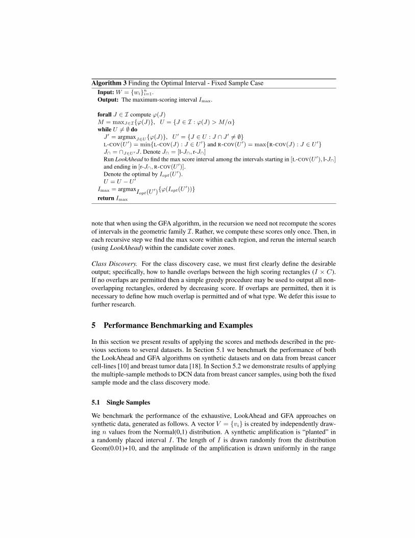
Algorithm 3 Finding the Optimal Interval - Fixed Sample CaseInput: W = {wi}n

i=1.Output: The maximum-scoring interval Imax.

forall J ∈ I compute ϕ(J)M = maxJ∈I{ϕ(J)}, U = {J ∈ I : ϕ(J) > M/α}while U 6= ∅ do

J ′ = argmaxJ∈U{ϕ(J)}, U ′ = {J ∈ U : J ∩ J ′ 6= ∅}L-COV(U ′) = min{L-COV(J) : J ∈ U ′} and R-COV(U ′) = max{R-COV(J) : J ∈ U ′}J∩ = ∩J∈U′J . Denote J∩ = [l-J∩, r-J∩]Run LookAhead to find the max score interval among the intervals starting in [L-COV(U ′), l-J∩]and ending in [r-J∩, R-COV(U ′)].Denote the optimal by Iopt(U

′).U = U − U ′

Imax = argmaxIopt(U′){ϕ(Iopt(U

′))}return Imax

note that when using the GFA algorithm, in the recursion we need not recompute the scoresof intervals in the geometric family I. Rather, we compute these scores only once. Then, ineach recursive step we find the max score within each region, and rerun the internal search(using LookAhead) within the candidate cover zones.

Class Discovery. For the class discovery case, we must first clearly define the desirableoutput; specifically, how to handle overlaps between the high scoring rectangles (I × C).If no overlaps are permitted then a simple greedy procedure may be used to output all non-overlapping rectangles, ordered by decreasing score. If overlaps are permitted, then it isnecessary to define how much overlap is permitted and of what type. We defer this issue tofurther research.

5 Performance Benchmarking and Examples

In this section we present results of applying the scores and methods described in the pre-vious sections to several datasets. In Section 5.1 we benchmark the performance of boththe LookAhead and GFA algorithms on synthetic datasets and on data from breast cancercell-lines [10] and breast tumor data [18]. In Section 5.2 we demonstrate results of applyingthe multiple-sample methods to DCN data from breast cancer samples, using both the fixedsample mode and the class discovery mode.

5.1 Single Samples

We benchmark the performance of the exhaustive, LookAhead and GFA approaches onsynthetic data, generated as follows. A vector V = {vi} is created by independently draw-ing n values from the Normal(0,1) distribution. A synthetic amplification is “planted” ina randomly placed interval I . The length of I is drawn randomly from the distributionGeom(0.01)+10, and the amplitude of the amplification is drawn uniformly in the range

Rnd1 Rnd2 Rnd3 Rnd4 Pol Hymn 1,000 5,000 10,000 50,000 6,095 11,994# of instances 1000 200 100 100 3 3Exhaustive 0.0190 0.467 1.877 57.924 0.688 2.687LookAhead 0.0045 0.044 0.120 1.450 0.053 0.143GFA 0.0098 0.047 0.093 0.495 0.079 0.125

Table 1. Benchmarking results of the Exhaustive, LookAhead and GFA algorithms on synthetic vec-tors of varying lengths (Rnd1-Rnd4), and six biological DCN vectors from [18] (Pol) and [10] (Hym).Running times are in seconds; simulations performed on a 0.8GHz Pentium III. For Hym and Pol datafrom all chromosomes were concatenated to produce significantly long benchmarks. LookAhead wasrun with κ =

√n, GFA with ε = 0.1. Linear regression to log-log plots suggest that running times

of the Exhaustive, LookAhead and GFA algorithms are O(n2), O(n1.5) and O(n), respectively.

[0.5, 10]. Synthetic data was created for four different values of n - 1,000, 5,000, 10,000,and 50,000. In addition, we applied the algorithms to six different biological DCN vec-tors from [18] and [10]. Benchmarking results of finding the maximum scoring interval aresummarized in Table 5. Note that the data from different chromosomes were concatenatedfor each biological sample to produce significantly long benchmark instances.

Figure 1 depicts high scoring intervals identified in chromosome-17, based on aCGHdata from a breast cancer cell line sample (MDA-MB-453 - 7723 probes). Here, all inter-vals with scores > 4 were identified, including nested intervals. Running time of the fullsearch dropped from 1.1 secs per sample with the exhaustive search, to 0.22 secs using therecursive LookAhead heuristic.

Fig. 1. Significant alterations in breast cancer cell line sample MDA-MB-453, chromosome 17 (7723probes, from [2]). The thin line indicates the raw data, smoothed with a 1Mb moving average window.Overlaid thick lined step function denotes the identified aberrations, where intervals above the x-axis

denote amplifications with score ϕsigS (I) > 4 and intervals below the x-axis – deletions with score

ϕsigS (I) < −4. The relative y-position of each interval indicates the average signal in the altered

interval.

5.2 Multiple Samples

Fixed Sample Set. We searched for common alterations in the two different breast can-cer datasets. We used ϕrob to detect common aberrations in a set of 14 breast cancer cellline samples (data from [10]). Figure 2 depicts the chromosomal map of common aberra-tions that were identified with a score of |ϕrob

S (I)| > 4.5. No intervals with scores of thismagnitude were located when the analysis was repeated on random data.

Class Discovery. We used scorerob to detect classes of common alterations in 41 breasttumor samples (data from [18]). A large number of significant common alterations wereidentified in this dataset, with significantly high intervals scores, ϕrob(I, C) > 12. Again,no intervals with scores of this magnitude were located when the analysis was repeated onrandomly permuted data. Some large aberrations were identified, including alterations af-fecting entire chromosomal arms as described in the literature [18]. Specifically, amplifica-tions in 1q, 8q, 17q, and 20q, and deletions in 1p, 3p, 8p, and 13q, were identified, as well asnumerous additional smaller alterations. Some of these regions contain known oncogenes(e.g. MYC (8q24), ERBB2 (17q12) , CCND1 (11q13) and ZNF217 (20q13)) and tumorsuppressor genes (e.g. RB (13q14), TP53 (17p13), BRCA1 (17q21) and BRCA2 (13q13)).Figure 2 depicts two significant common alterations that were identified in 8p (deletion)and 11q (amplification). An interesting aspect of the problem, which we did not attempt toaddress here, is the separation and visualization of different located aberrations, many ofwhich contain significant intersections.

Fig. 2. a) Common alterations detected in 14 breast cancer cell line samples (data from [10]), in fixedset mode. All alterations with score |ϕrob

S (I)| > 4.5 are depicted - amplifications by red marks,and deletions by green marks. Dark blue marks denote all probe positions. b) Common deletion in8p (ϕrob(I, C) = 23.6) and common amplification in 11q (ϕrob(I, C) = 22.8) identified in twosubsets of 41 breast cancer samples in class discovery mode, τ = 0 (data from [18]). X-axis denoteschromosomal position. Samples are arbitrarily ordered in y-axis to preserve a different class structurefor each alteration. Red positions denote positive values and green – negative values.

References1. B.R. Balsara and J.R. Testa. Chromosomal imbalances in human lung cancer. Oncogene,

21(45):6877–83, 2002.2. M.T. Barrett, A. Scheffer, A. Ben-Dor, N. Sampas, D. Lipson, R. Kincaid, P. Tsang, B. Curry,

K. Baird, P.S. Meltzer, Z. Yakhini, L. Bruhn, , and S. Laderman. Comparative genomic hybridiza-tion using oligonucleotide microarrays and total genomic DNA. PNAS, 101(51):17765–70, 2004.

3. G. Bignell, J. Huang, J. Greshock, S. Watt, A. Butler, S. West, M. Grigorova, K. Jones, W. Wei,M. Stratton, P. Futreal, B. Weber, M. Shapero, and R. Wooster. High-resolution analysis of DNAcopy number using oligonucleotide microarrays. Genome Research, 14(2):287–95, 2004.

4. C. Brennan, Y. Zhang, C. Leo, B. Feng, C. Cauwels, A.J. Aguirre, M. Kim, A. Protopopov,and L. Chin. High-resolution global profiling of genomic alterations with long oligonucleotidemicroarray. Cancer Research, 64(14):4744–8, 2004.

5. M.H. DeGroot. Probability and Statistics, chapter 5.7, page 275. Addison-Wesley, 1989.6. W. Feller. An Introduction to Probability Theory and Its Applications, volume I, chapter VII.6,

page 193. John Wiley & Sons, 1970.7. K.S. Fu and J.K. Mui. A survey of image segmentation. Pattern Recognition, 13(1):3–16, 1981.8. J. Himberg, K. Korpiaho, H. Mannila, J. Tikanmki, , and H.T.T. Toivonen. Time series segmen-

tation for context recognition in mobile devices. In Proceedings of the 2001 IEEE InternationalConference on Data Mining (ICDM 2001), pages 203–210, 2001.

9. P. Hupe, N. Stransky, J.P. Thiery, F. Radvanyi, and E. Barillot. Analysis of array CGH data: fromsignal ratio to gain and loss of DNA regions. Bioinformatics, 2004. (Epub ahead of print).

10. E. Hyman, P. Kauraniemi, S. Hautaniemi, M. Wolf, S. Mousses, E. Rozenblum, M. Ringner,G. Sauter, O. Monni, A. Elkahloun, O.P. Kallioniemi, and A. Kallioniemi. Impact of DNAamplification on gene expression patterns in breast cancer. Cancer Research, 62:6240–5, 2002.

11. O.P. Kallioniemi, A. Kallioniemi, D. Sudar, D. Rutovitz, J.W. Gray, F. Waldman, and D. Pinkel.Comparative genomic hybridization: a rapid new method for detecting and mapping DNA am-plification in tumors. Semin Cancer Biol, 4(1):41–46, 1993.

12. D. Lipson, A. Ben-Dor, E. Dehan, and Z. Yakhini. Joint analysis of DNA copy numbers andexpression levels. In Proceedings of WABI 04, LNCS. Springer, 2004. In press.

13. F. Mertens, B. Johansson, M. Hoglund, and F. Mitelman. Chromosomal imbalance maps of ma-lignant solid tumors: a cytogenetic survey of 3185 neoplasms. Cancer Research, 57(13):2765–80, 1997.

14. M. Morley, C. Molony, T. Weber, J. Devlin, K. Ewens, R. Spielman, and V. Cheung. Geneticanalysis of genome-wide variation in human gene expression. Nature, 430(7001):743–7, 2004.

15. D. Pinkel, R. Segraves, D. Sudar, S. Clark, I. Poole, D. Kowbel, C. Collins, W.L. Kuo, C. Chen,Y. Zhai, S.H. Dairkee, B.M. Ljung, J.W. Gray, and D.G. Albertson. High resolution analysis ofDNA copy number variation using comparative genomic hybridization to microarrays. NatureGenetics, 20(2):207–211, 1998.

16. P. Platzer, M.B. Upender, K. Wilson, J. Willis, J. Lutterbaugh, A. Nosrati, J.K. Willson, D. Mack,T. Ried, and S. Markowitz. Silence of chromosomal amplifications in colon cancer. CancerResearch, 62(4):1134–8, 2002.

17. J.R. Pollack, C.M. Perou, A.A. Alizadeh, M.B. Eisen, A. Pergamenschikov, C.F. Williams, S.S.Jeffrey, D. Botstein, and P.O. Brown. Genome-wide analysis of DNA copy-number changesusing cDNA microarrays. Nature Genetics, 23(1):41–6, 1999.

18. J.R. Pollack, T. Sorlie, C.M. Perou, C.A. Rees, S.S. Jeffrey, P.E. Lonning, R. Tibshirani, D. Bot-stein, A. Borresen-Dale, and P.O. Brown. Microarray analysis reveals a major direct role ofDNA copy number alteration in the transcriptional program of human breast tumors. PNAS,99(20):12963–8, 2002.

19. J. Sebat. Large-scale copy number polymorphism in the human genome. Science,305(5683):525–8, 2004.

A Proof of Theorem 1

Let f : R → R be a strictly concave function (that is tf(x)+(1−t)f(y) < f(tx+(1−t)y)for all 0 < t < 1). We define the score of an interval I with respect to f , denoted Sf (I), tobe the sum of I’s entries divided by f(|I|). In particular, for f(x) =

√x, S(I) coincides

with the interval score function we use throughout this paper.For a given vector of real numbers, of length n, let m > 0 denote the maximal interval

score obtained (among all(n2

)intervals). We call an interval optimal if its score equals m.

The following theorem bounds the number of optimal intervals:

Theorem 4. There can be at most n optimal intervals.

Claim. For all x, y > z > 0 the following inequality holds: f(x) + f(y) > f(z) + f(x +y − z)

Proof. Define t = (x− z)/(x + y − 2z). Note that

x = t(x + y − z) + (1− t)z, and y = tz + (1− t)(x + y − z).

As f is strictly concave, and 0 < t < 1

tf(x + y − z) + (1− t)f(z) < f(t(x + y − z) + (1− t)(z)) = f(x)tf(z) + (1− t)f(x + y − z) < f(t(z) + (1− t)(x + y − z)) = f(y)

Summing the above two inequalities, we get

f(x + y + z) + f(z) < f(x) + f(y)

Claim. If two optimal intervals I and J intersect each other than either I properly containsJ or vise versa.

Claim. If two optimal intervals I and J are disjoint, there must be at least one point be-tween them which is not included in either. Otherwise, consider the interval K = I; Jrepresenting their union.

Let I be a collection of optimal intervals. For each x ∈ {1, . . . , n} we denote by I(x)the set set of optimal intervals that contains x.

Claim. All intervals in I(x) have different sizes.

Proof. Any two optimal intervals that contains x intersect. By Claim A one of them prop-erly contains the other. Thus, they have different size.

We define for each x the smallest interval that contains x, denoted by T (x). Note thatby the previous claim, there can be only one minimal interval that contains x. To completethe upper bound proof, we show now that the mapping T : {1, . . . , n} ← I is onto.

Lemma 3. For each optimal interval I there exist a point x such that T (x) = I .

Proof. Let I be an optimal interval, I = [i,←, j]. We consider two cases

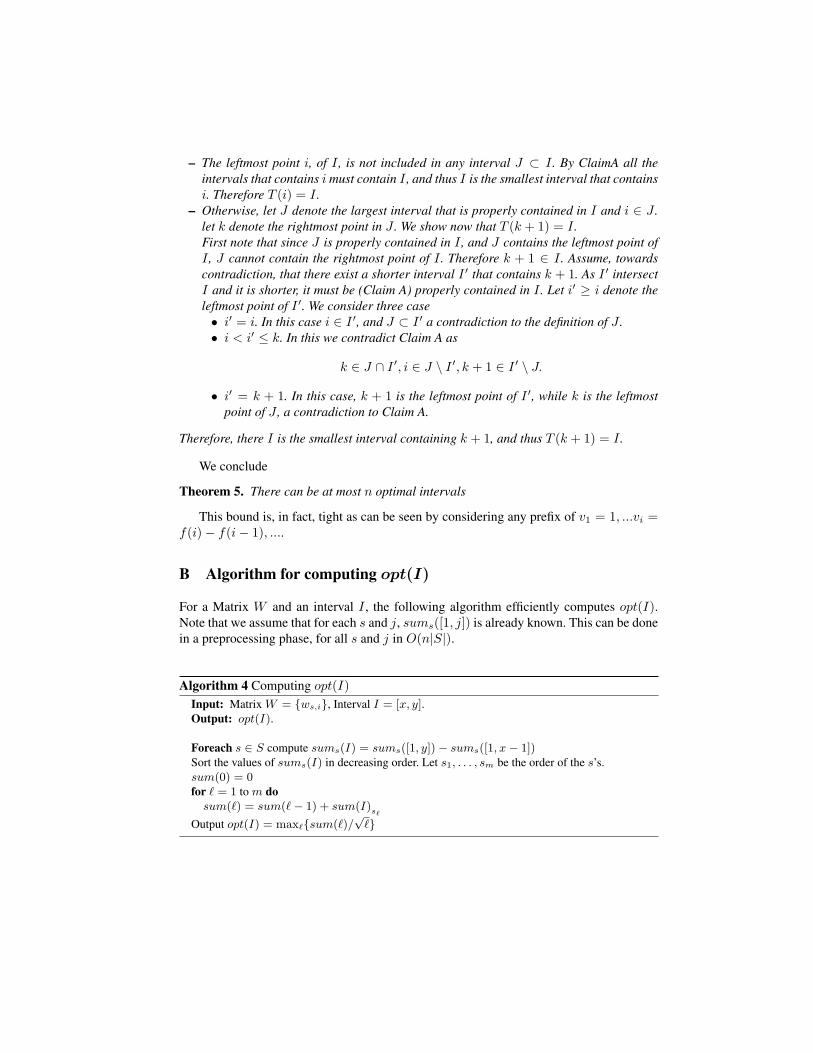
– The leftmost point i, of I , is not included in any interval J ⊂ I . By ClaimA all theintervals that contains i must contain I , and thus I is the smallest interval that containsi. Therefore T (i) = I .

– Otherwise, let J denote the largest interval that is properly contained in I and i ∈ J .let k denote the rightmost point in J . We show now that T (k + 1) = I .First note that since J is properly contained in I , and J contains the leftmost point ofI , J cannot contain the rightmost point of I . Therefore k + 1 ∈ I . Assume, towardscontradiction, that there exist a shorter interval I ′ that contains k + 1. As I ′ intersectI and it is shorter, it must be (Claim A) properly contained in I . Let i′ ≥ i denote theleftmost point of I ′. We consider three case• i′ = i. In this case i ∈ I ′, and J ⊂ I ′ a contradiction to the definition of J .• i < i′ ≤ k. In this we contradict Claim A as

k ∈ J ∩ I ′, i ∈ J \ I ′, k + 1 ∈ I ′ \ J.

• i′ = k + 1. In this case, k + 1 is the leftmost point of I ′, while k is the leftmostpoint of J , a contradiction to Claim A.

Therefore, there I is the smallest interval containing k + 1, and thus T (k + 1) = I .

We conclude

Theorem 5. There can be at most n optimal intervals

This bound is, in fact, tight as can be seen by considering any prefix of v1 = 1, ...vi =f(i)− f(i− 1), ....

B Algorithm for computing opt(I)

For a Matrix W and an interval I , the following algorithm efficiently computes opt(I).Note that we assume that for each s and j, sums([1, j]) is already known. This can be donein a preprocessing phase, for all s and j in O(n|S|).

Algorithm 4 Computing opt(I)Input: Matrix W = {ws,i}, Interval I = [x, y].Output: opt(I).

Foreach s ∈ S compute sums(I) = sums([1, y])− sums([1, x− 1])Sort the values of sums(I) in decreasing order. Let s1, . . . , sm be the order of the s’s.sum(0) = 0for ` = 1 to m do

sum(`) = sum(`− 1) + sum(I)s`

Output opt(I) = max`{sum(`)/√

`}