COMPONENTS OF THE EXCHANGE RISK PREMIUM IN A MULTIPLE DEALER FX MARKET

Alexis Derviz1

ABSTRACT

The paper proposes a continuous time model of an FX market organized as a multiple dealership. The dealers have costly access to best available quotes. They interpret signals from the joint dealer-customer order flow and decide upon their own quotes and trades in the inter-dealer market. Each dealer uses the observed order flow to improve the subjective estimates of relevant aggregate variables, which are the sources of uncertainty. These are: returns on domestic and foreign assets, the equilibrium FX transaction price and the size of the cross-border dealer transactions in the FX market. These uncertainties have diffusion form and are dealt with according to the principles of portfolio optimization in continuous time. The model is used to explain the country, or risk, premium in the uncovered national return parity equation for the exchange rate. The two country premium terms that I identify in excess of the usual covariance term (consequence of the �Jensen inequality effect�) are: the dealer heterogeneity-induced inter-dealer market order flow component and the dealer Bayesian learning component. As a result, a �dealer-based total return parity� formula links the exchange rate to both the �fundamental� factors represented by the differential of the national asset returns, and the microstructural factors represented by heterogeneous dealer knowledge of the aggregate order flow and the fundamentals. Keywords: FX microstructure, optimizing dealer, diffusion uncertainty, uncovered parity JEL Classification: F31, G11, G29, D49, D82

1 The Czech National Bank, Monetary and Statistical Dept., Na Prikope 28, CZ-115 03 Praha 1, Czech Republic, E-mail: Alexis.Derviz@cnb.cz .

2

1. Introduction2 The paper develops a continuous time model of the inter-dealer FX market and derives consequences for the risk premium structure in the formula for uncovered parity of national asset returns. I demonstrate that the forex microstructure has an impact on the dynamics of the risk premium, by linking the behavior of the latter to (1) the order flow received by dealers-domestic residents from other market users (2) errors in the dealers� assessments of the aggregate cross-border order flow and economic

fundamentals. The model allows one to address two types of FX market effects. The first are the �long-run� properties of the exchange rate, such as a (generalized) uncovered parity or competitive quoting by multiple dealers around a clearing price. The second group, which is more short-run by nature, refers to information extraction procedures and Bayesian belief updating by participants in the inter-dealer market in the face of changing fundamentals. Combining the said objectives, I use the model to derive a �dealer-based� uncovered parity of national asset returns with respect to the expected exchange rate return. This parity theorem contains the country premium term that depends on the order flow from non-resident market users to resident dealers. One term in the premium is present under both perfect and imperfect information and comes from liquidity needs resulting from dealer heterogeneity. The other term arises as a consequence of imperfect information of an individual dealer about the aggregate order flow and national asset return statistics. Bayesian learning and belief updating by the dealers then leads to long-lasting shifts in the country premium. The result obtained in this paper generalizes the uncovered parity property of the exchange rate that comes up naturally in any optimizing model of international asset pricing. (Under the Walrasian market clearing assumption, this uncovered parity would follow from the international consumption-based CAPM.) We choose to call it the uncovered total return parity (UTRP), to make a distinction from the much-compromised uncovered interest rate parity of naïve no-arbitrage models. UTRP associates the exchange rate expectations for a given period with the difference in total returns (instantaneous dividend over price plus capital gain) on a pair of representative securities. These total returns coincide with yields to maturity in continuous time. Accordingly, the return quoted in a secondary market and not the money market loan/deposit rate, which is pre-determined for the time interval in question, constitutes the continuously updated measure of the expected move in the exchange rate (see Derviz, 2002, for details, including empirical verification of UTRP). This parity theorem would be valid exactly and permanently in a Walrasian auctioneer setting which ignores microstructure, with a representative agent and markets clearing at each moment. However, when one studies the exchange rate formation in a dealership market, deviations from the fundamental UTRP come about as a natural consequence of agent heterogeneity. These deviations reflect information and inventory flows between dealers and investors. The proposed model establishes a link between an individually observed order flow, Bayesian filtering of imprecisely known fundamentals by the dealer, and the seemingly unwarranted variability of the country premium in the UTRP formula. The model predicts that deviations from UTRP should be most pronounced at times when some dealers are learning new information from their clients through the observed order flow. During such periods,

2 Comments and valuable advice by Rich Lyons from the Haas School, U.C. Berkeley, Charles Goodhart from LSE, Carol Osler from the New York FED, and Martin Evans from Georgetown Univ., are gratefully acknowledged. The usual disclaimer applies.

3

1. The exchange rate and the inter-dealer order flow variability must be higher than under complete symmetric information

2. Dynamic processing of new signals by the dealers leads to deviations from UTRP that persist until the new information has been absorbed; under certain circumstances, Bayesian learning by the dealers can lead to a permanent revision of the country premium level in the uncovered parity relation.

In this sense, the model describes situations in which the order flow effects are long-lived. To highlight the �right� price discovery process starting with the end-users of the foreign currency (investors) and going through the dealers who learn from them, the existing microstructure literature usually makes a conceptual distinction between clients and dealers. This happens both in single dealer sequential trade models of Glosten and Milgrom, 1985, or Easley and O�Hara, 1987, with a single risk-neutral market maker, and in multiple dealer models of the Evans and Lyons, 1999, type. This distinction is barely possible in practice. More importantly, the real life roles of the investor and dealer in the FX market are often combined in the performance of cooperating parts within the same company. Most typically, a major commercial or investment bank has dealers who service its customers and participate in the inter-dealer market, but also operates proprietary trading desks that exercise FX transactions for the needs of its own portfolio management. Access to electronic cross-border security trade and information systems is not a privilege of dealers either: the community of Reuters and/or Bloomberg quote screen users includes a considerable part of the internationally active companies of very versatile profiles. Access to these facilities becomes highly attractive to any company whose cross-border operations attain a certain size. Accordingly, most of available price and trade size data carry no stamp of the purpose of any given FX-transaction. One of the exceptions in the literature in terms of client-dealer separation is the paper by Madhavan and Smidt, 1993, in which a dealer is also an active investor. Similarly to Madhavan and Smidt, I model a synthetic dealer-investor. All agents in the present model are market users. They can be either local, trading only with one selected dealer, or global, having access to the inter-dealer market. That is, global market users are able to both search for the best dealer quotes and exercise a trade with the dealer of their choice. The only distinction between dealers and the rest of the global market users is that the former assume the market making function. Apart from that, dealers have the same intrinsic motive for holding foreign currency positions as any other market user, since they are active in the same lines of international business as the latter. The respective roles of local and global market users in the model can be roughly summarized as follows: order flow of the locals creates noise and can generate exogenous asymmetry in dealer positions; order flow of the globals acts as a signal that transmits information between dealers.3 The majority of information-oriented forex microstructure models define the signals as unbiased estimates of some �true� or �fundamental� value of the exchange rate. Apparently, this feature was inherited from microstructure studies of other markets (e.g. equities, where this true value is associated with revealed earnings or dividend data). However, in the case of

3 This understanding of the aggregate signaling effects of the market users� order flow can be supported by the reference to the model of Bernhardt and Hughson, 1997. There, customers are splitting orders between dealers to equalize marginal benefits from trade at different pricing schedules. The implicit marginal benefits equalization is the reason why, in our model, the global market user order flow observed by one dealer contains information on the order flow received by other dealers, as well.

4

the exchange rates, no such revelation of absolute truth exists. Instead, I let the signals reaching the dealers contain information about the �other side of the market�, i.e. the aggregate behavior of the received trades initiators. This allows us to close the model in a natural way. I am not modeling either pure �information� or pure �inventory� motives for trade, but rather, an �information about inventory� motive. Another highly stylized feature of existing models of the inter-dealer market is a strict sequencing of information-laden events in them. (Cf. Evans and Lyons, 1999: first a round of dealer trades with customers signaling fundamental information, then an inter-dealer round to redistribute inventory risk between dealers, then another round of customer trades to unwind open positions.) On the contrary, data on FX trades of a given financial institution reflect three simultaneously evolving random processes pertaining to own investment needs, the inter-dealer and the customer-dealer operations. In other words, at each moment, the dealer observes the three named categories of transactions simultaneously and has to exercise a belief update based on these observations. Under such conditions, a continuous time stochastic model of the dealer behavior appears to be the most convenient. A non-negligible argument in favor of a continuous time dealer model with diffusion uncertainty is its better analytical tractability compared to discrete time models with arbitrary statistics of risk factors. There already exists a line of literature that develops the findings of the Kyle, 1985, risk-neutral market maker model in continuous time. For example, Back, 1992, Back and Pedersen, 1998, and Back, Cao and Willard, 2000, work with price and cumulative orders in a security market (applicable to forex) in semimartingale form, with diffusion components originating in the action of noise traders. When one considers optimizing models for risk-sensitive agents, the stochastic maximum principle becomes an even more powerful tool of analyzing the equilibrium price and order flow dynamics in continuous time, once the dealer optimization problem is properly defined in this setting. The crucial challenge here is to identify and interpret the information asymmetry and Bayesian belief updating phenomena and their role in the obtained solutions.4 This task in a continuous time portfolio model of the Cox-Ingersoll-Ross type with heterogeneous beliefs was first addressed by Detemple, 1986. Zapatero, 1998, used the same approach to derive results on asset price volatility under asymmetric information in continuous time. Since each dealer has a local customer base that trades with him exclusively, there is enough space for a non-trivial bid-ask spread in his quotes. The adverse selection reason for the existence of spreads identified in most models with informationally heterogeneous traders, namely the compensation of losses from trades with the informed by profits made in trades with the uninformed, is implicitly present in this setting as well. The role of the informed is played by the global traders, while that of the uninformed is played by the local traders. The latter, when they trade at given spreads, are subject to the exercise of monopoly power by their dealer. This understanding is close to the ideas of Copeland and Galai, 1983, and Perraudin and Vitale, 1996. However, the present model generates non-trivial � and variable � bid-ask spreads even when there is more than one dealer in the market. The existence of global investors extends the competition from pure inter-dealer interaction to the area of dealer-customer relations.

4 The previously mentioned continuous time models of FX trade by Back and colleagues are based on Kyle�s auctioneer and do not include dealers explicitly. Besides, these models abstract from the usual Brownian asset return uncertainties faced by an investor and concentrate on the market interpretation of narrowly defined exogenous signals about the foreign currency value.

5

The existence of informational heterogeneity between investor groups of different residences is pivotal in generating non-trivial order flows and additional sources of exchange rate volatility in our model. This type of heterogeneity has already found reflection in finance literature. For instance, Brennan and Cao, 1997, argue that asymmetry between domestic and foreign investors in the knowledge of domestic asset returns has an impact on the direction and volume of cross-border equity trade. More specifically, a recent working paper by Seasholes, 2000, argues that large foreign investors in emerging markets have an informational advantage and cash in higher returns on domestic equity, compared to the majority of domestic investors. (Therefore, cross-border informational asymmetry does not always mean an advantage for residents.) Our model shares the Brennan and Cao view that residency-based informational heterogeneity matters, but also allows for difference in informational endowments between local and global investors, in accordance with the Seasholes conjecture. The paper is structured as follows. Section 2 describes the model variables, the structure of uncertainty and the dealer�s optimization problem (Subsection 2.1), after which the optimal dealer strategies for passive (at own quotes) and active (at other dealers� quotes) FX trades are derived (Subsection 2.2). I also show how a non-zero bid-ask spread and a competitive mid-quote arise as a result of dealer optimization. Section 3 analyzes the long-run FX transaction price dynamic resulting from the uncovered total return parity. Section 4 discusses order-flow interpretation and updating of beliefs by dealers, leading to deviations from the uncovered parity of returns. It also presents some FX data that support the conclusions of the model. Section 5 concludes and indicates possibilities for future research. 2. The investor-dealer decision problem 2.1 The model The world is split into the home country with legal tender M and the foreign country with legal tender I. By the exchange rate, we understand the price of I in M-terms. Investors residing in the home country account their operations in M, those residing in the foreign country use the accounting unit I.5 Among the investors (of both residencies), there is a subset of those who offer forex dealer services to the others. That is, they agree to provide an ask quote pa which is the price at which they agree to sell I in exchange for M, and a bid price pb at which they agree to buy I in exchange for M. We will call them investor-dealers or simply dealers. Each dealer has a local customer base of those investors who only exercise FX trades through him at given quotes (they are free to vary the traded quantity from zero to infinity depending on the quotes they see). Alongside them, there are other (global) investors who are able to search for the best quote among all dealers, at a cost. Each dealer also has the ability of costly discovery of the best quote among other dealers. One would expect the investor-dealers to face a lower cost of quote search than investors without the dealing capacity. On the other hand, the non-dealer investors have priority in learning the news about fundamentals, to be discussed in Section 4. This balance between costs and benefits of market making should provide an intuitive justification for the existence of dealers in the model. In the case of a small FX market (e.g. a European currency not belonging to the euro zone or an emerging economy currency), one can loosely associate global investors with multinationals and international financial corporations present in the local economy. 5 The present model will accommodate the Jensen inequality-related properties of the expected exchange rate returns (will be free of the residency-based asymmetry of the latter, arising in naïve no-arbitrage settings and known as Siegel�s paradox). See Derviz, 2002, for the details of Siegel�s paradox resolution in the corresponding class of models.

6

Altogether, the order flow that a dealer observes consists of three parts. The first is the supply of I or demand for I from his local customers, dependent only on his own quote values pa and pb and the economic fundamentals influencing the customer base. This flow is unobserved by other parties. The remaining two order flow components come from the inter-dealer market. These are the orders of those (a) global investors and (b) other dealers, whose quote search has resulted in the choice of this dealer for the desired trade in the given period. For every party involved, participation in the inter-dealer market is a source of an information update about the statistics of the fundamental variables and the market-wide order flow, read off the received trades. The inter-dealer market is only partially transparent in the sense that each participant only observes his/her own trades, whereas the knowledge of standing best quotes is the result of a costly search for each outgoing trade. These search costs are a part of the overall transaction costs (to be defined below). One can think of an agent with access to electronic and voice brokers who service parts of the market, but who is not sure whether a better price could be found by approaching certain dealers individually. While not modeling these tradeoffs between a broker and individual search explicitly, we adopt the understanding that the best price can always be found, even if the resources dedicated to the search grow faster than the desired transaction amount. The international investor exercising the function of an FX-dealer will be modeled as an agent characterized by four state variables. These are: x0 � domestic cash holdings, xd � holdings of the composite domestic asset, xi � foreign cash holdings, xf � holdings of the composite foreign asset. The domestic asset pays out a random rate of return drd in M-units. I also assume that maintaining the investment portfolio xd requires continuous inputs of funds (management costs) without which the value xd deteriorates at a stochastic rate dαd. (This is done for the sake of convenience, allowing one to consider equilibria with constant average levels of asset holdings.) Let one unit of xd cost Xd units of M. Analogous values for the foreign investment portfolio are denoted by drf, dαf and Xf, respectively (the latter price is in I-units). Cash holdings x0 and xi earn their own rates of return dr0 and dri, respectively. In the simplest variant, it can be the overnight money market rate (or its proportional part if the elementary period is intra-day). More realistically, one should include in the cash variables the inter-bank loan/deposit positions and FX swap positions. In that case, dr0 (dri) is the instantaneous rate paid in the domestic (foreign) money market on the corresponding portion of x0 (xi), i.e. the generator short rate of the domestic (foreign) term structure. For any strictly positive Itô process z, dz/z will be a shortened to zd

). The drift and diffusion

coefficients of the asset return and price processes introduced above will be denoted as follows:

dZIdtidr dd +=0 , dZIdtidr ffi += , dZNdtndr ddd += , dZNdtndr fff += , dZAdtad ddd +=α , dZAdtad fff +=α , dZdtXd ddd ρπ +=

), dZdtXd fff ρπ +=)

. Since it is not the purpose of this paper to study GARCH or other non-constant variance effects in asset prices, all diffusion coefficients I, N, A and ρ are assumed constant.

7

Itô processes r0, rd, ri, rf, αd and αf belong to the exogenous sources of uncertainty in the model. Jointly, these processes, together with two more to be introduced in Subsection 2 and Section 4, respectively, generate the information filter F=(Ft)t≥0 to which all stochastic processes appearing in the model will be adapted. (Ft denotes the partition of the event space corresponding to the full information about the operation of the markets, on which the objective probability measure valid at time t is defined.) Let the diffusions adapted to F be spanned by a vector Z of mutually independent standard Brownian motions. Current FX transaction price We have assumed that the global market users (dealers or not) are allowed to search in the inter-dealer market for acceptable quotes. Next, we introduce the notion of the best attainable bid and ask prices for a given dealer, Pb and Pa, good for one unit of I. Trade size-dependent non-linearities will be accommodated by means of convex transaction costs (see below). Assumption 1 For each global investor and each dealer, the best individually attainable (highest) bid price is equal to the best attainable (lowest) ask price: Pb= Pa=P, i.e. the inside spread/touch is zero. Although, in reality, the touch is positive, it is very small under normal circumstances (i.e. unless markets become turbulent). Goodhart et al., 1996, observe that interdealer FX spreads on major currency pairs are usually as tiny as 1 pip or 1/10 of the basis point for standard amounts. These are the numbers reported by the Reuters D2000-2 electronic brokerage system, i.e., the inside spreads, giving a perfect match with Assumption 1 (which just sets the minimal �technical� touch amount to zero for simplicity). On the theoretical side, the inside spread diminishing with the number of competing dealers is one of the outcomes of the model by Ho and Stoll, 1983. Their model also predicts that spreads of individual dealers would not fall to zero even when their number becomes large. This is in line with the results to be obtained in the present paper. More generally, the intuitive justification of Assumption 1 is related to the information-dissemination ability of the modeled competitive inter-dealer market. If one observed Pb >Pa, then there would be a clear arbitrage opportunity. In the opposite case Pb< Pa, there would be no inter-dealer trades at all until the too high asks went down and/or the too low bids went up to meet each other and provide gains from trade to those who seize the opportunity. There shall always be an agent who discovers the deadlocked market and undercuts/overbids the standing quote in his favor. As soon as all the arbitrage and market share appropriation possibilities have been exhausted, there remains a group of inter-dealer market sellers and another group of buyers. They transact at the mutually acceptable price P. The buyers� ask price and the sellers� bid price quotes are non-competitive: above P in the first group and below P in the second. Therefore, the buyers do not have to sell and the sellers do not have to buy.6 The dealer population is split into sellers and buyers at every given moment. One reason why someone becomes a seller and someone else a buyer is the heterogeneity of asset endowments. Even in the absence of the latter, there is a possibility of differences in privately accounted net returns on assets between dealers. For instance, foreign residents may have a handicap with regard to domestic asset management, including noisy information on returns, taxation or profit repatriation costs, and vice versa. Domestic dealers may enjoy privileged

6 Thus, the present model incorporates the observation by Silber, 1984, that dealers are typically competitive on only one side of the market.

8

access to the domestic money market, with a resulting higher return on domestic cash balances, and a symmetric advantage may be enjoyed by foreign residents with respect to foreign cash. All the named factors can be exacerbated by heterogeneity of beliefs (see Section 4). The last-observed inter-dealer transaction price P will be identified with the market price. It is the one used in the dealer�s accounting. Each agent views it as a strictly positive Itô process with coefficients defined by dZdtPd ρπ +=

).

Investment performance measure For the later purpose of defining preference over the paths of investor-dealer�s actions, we are introducing the notional dividend rate δ to be accounted for in every infinitesimal period dt. Our model shall be able to work with very short time steps (such as those of the real-time data of electronic FX-trade systems). In this case, the defined dividend rate shall be understood as an imaginary infinitesimal contribution of the dealer department to the dividend fund of the firm, whose integral, in reality, is being withdrawn from the cash balance at discrete intervals. Having this infinitesimal dividend rate in the model is a convenient way to make the dealer accountable for the ultimate performance of the forex activity of the firm, and, at the same time, bring the preference structure of the agent close to the standard portfolio optimization setups. Price search costs In order to generate non-trivial supply and demand schedules (for instance, Glosten, 1989, uses non-linear pricing schedules in his investor-dealer game in both monopolistic and competitive dealer settings) facing the other side of the market, it is usual to define transaction costs that grow in a convex way in the transaction volume. It is well known that observable transaction costs incurred by a big real-life investor, let alone a dealer, are usually negligible for small/standard amounts, but grow rapidly when the trade size exceeds the standard. Accordingly, non-linear pricing schedules are a reality. In addition, some form of generalized transaction costs seems to lie behind the dealer behavior, even if these costs are not readily measured. In this paper, we take the view that these costs include the cost of a quote search in the inter-dealer market. Specifically, let us assume that in order to buy/sell volume vidt of I at market price P (which is the last observed highest bid if vi<0 and the last observed lowest ask if vi>0), one pays/receives Pk(vi)dt units of M. Here, k is a strictly increasing and strictly convex function with 1)0( =′k . A natural example would be a quadratic function of the form

k(v)=v+k0v2/2. For consistency reasons, one should assume the same search cost mechanism to be present in the two other market segments as well. That is, if amounts vd and vf of the domestic and foreign asset are purchased per period (sold if negative), the M- and I-balances are reduced by amount Xd dtvk d )( and Xf dtvk f )( , respectively. The dealer�s order flow As was mentioned in the introduction, it is difficult to obtain separate data on the customer and inter-dealer components of a dealer�s order book. Instead, we distinguish between the local customers of the given dealer (do not have access to or exercise FX trades with others) and the participants of the inter-dealer market. Both the global investors who search among available dealer quotes and dealers themselves belong there. Accordingly, the pair of ask and

9

bid I-prices pa, pb, announced by the dealer, shall service everyone at the moment of announcement. However, we assume that the dealer is able to distinguish between a locally riskless (non-diffusion) demand D(pa)dt, a locally riskless supply S(pb)dt, and a random flow, which can go both ways, x0dΛ/P=x0(ldt+λdZ)/P, generated by Itô process Λ with drift l and diffusion λ. Altogether, the accounted change in the dealer�s M-balance, induced by trades at his quotes, is equal to

( ) ( ) ( ) Λ+−=++− dxdtpSppDpdZldtxdtpSppDp bbaabbaa 00 )()()()( λ , (1)

while the corresponding change in the I-balance is

[ ] ( ) [ ] Λ−−=+−− dPxdtpDpSdZldt

PxdtpDpS abab

00

)()()()( λ . (2)

Observe, in particular, the last diffusion terms in (1) and (2) coming from the diffusion part of

Λ: x0λdZ and dZPx λ

0

− . They reflect the dealer�s uncertainty about the order flow from both

global investors and other dealers. Indeed, one can generate the dealer�s diffusion-type order flow as a limit of two small-interval discrete flows of very small purchases at pa and very small sales at pb with a non-zero degree of randomness in the direction of the trade and its exact magnitude. Then the drift parts of the limit flows will correspond to the demand and

supply that are certain during the infinitesimal interval dt, namely dtPlxpD

aa

+

0

)( and

dtPlxpS

bb

−

0

)( , where la+lb=l. The diffusion part reflects the remaining uncertainty.

Considering the dealer an M-resident, we account for the random order flow in M-terms by expressing it as a stochastic growth rate of the M-cash account x0. It can be shown that the I-position in that case evolves exactly as is shown by the last term in equation (2)7. The

presence of the x0-proportional part Plx 0− in the drift component of the order flow is

explained by the possibility of the probability revision by the dealer (the drift change in Λ in accordance with the Girsanov theorem, see Elliott, 1982). The consequences of such a probability measure change in the case of a Bayesian update of beliefs will be discussed in Section 4. If the dealer were a foreign resident, the uncertain parts of the order flow that she faces would be xi-proportional, and the certain FX supply- and demand-entries in equations (1), (2), coming from the local customers, should be modified accordingly. Summing up the definitions given above, we come to the following system of state-transition equations for the state vector x=[x0,xd,xi,xf]T of an international investor with the dealer function (with domestic residence): 7 The said transition to the limit of discrete processes is a generalization of the well-known procedure of generating a geometric Brownian motion as a limit of random walks with a drift, when the step size goes to zero, see e.g. Dixit and Pindyck, 1994, Section 3.2.

10

( )dtpSppDpdtvPkdtvkXdtdrxdrxdx bbaaidddd )()()()(000 −+−−−+= δ ( )dZldtx λ++ 0 , (3a)

dtvdxdx dddd +−= α , (3b)

[ ] ( )dZldtPxdtpDpSdtvdtvkXdrxdrxdx abiffffiii λ+−−++−+=

0

)()()( , (3c)

dtvdxdx ffff +−= α . (3d) Preferences The introduced continuous time model is intended to be applicable to high frequency, such as daily or intra-day data. With such short time steps, it is not obvious whether a time preference/discount factor of the standard optimization models is applicable. Earlier, the dividend rate δ in equation (3a) was defined as an instantaneous contribution to the dividend fund, to be integrated over a finite time period. Let there exist a function u satisfying the conventional growth and concavity conditions, such that u(δ) measures the period utility (of the shareholders), derived from receiving contribution δ to the dividend fund. Similarly, infinitesimal rates dr and dα of asset return and deterioration in the model can be understood as the per-period contributions to the integral expected returns over a finite period (the drift parts) and unexpected innovations in these integral returns (the diffusion parts). Accordingly, an instantaneous time preference rate can be defined as an infinitesimal contribution to an integral discount factor valid for a finitely distant period in the future. Another possibility to be exploited here is to understand this rate, denoted by β, as the parameter of a Poisson �death� process. The present model neither requires a dealer to close the FX position in a predetermined finite time, nor does it rely on the existence of an exogenous final/underlying value of the currency. Instead, the following construction will replace the artificial shortcut of the �true liquidation value under discovery�, often utilized in microstructure models. For each time moment t, the dealer will have to close down his forex trade business within the next time interval dt, with probability 1-eβdt, and liquidate the outstanding engagement in currency I at current prices. The result of liquidation, i.e. the balance x0+Pxi, is evaluated by means of a strictly increasing and concave exit (or bequest) utility function G. As a result, at any time t the domestically resident dealer maximizes

( ){ }

++∫

∞−−

tt

issss

ts FdsxPxGueE 0)( )( βδβ (4)

with respect to control path ( )f

sis

dss vvvs ,,,δa , s≥t, subject to (3), given the current values xt

of asset holdings. Note the appearance of parameter β in front of G in the integrand in (4). Since, in each period ds, the firm liquidates with probability 1-e-βds, the expected utility derived from the liquidated position is equal to

( ) dsGdsGdseGe ss

ds

sds β

ββ ≈−=−

−− 11 .

If the dealer resides abroad, her liquidation balance entering G shall be accounted for in I-

units and be defined as ixPx +

0

. In either case, we shall assume that G decreases to -∞ when

11

cash balances become increasingly negative. Then, the presence of G in the period utility prohibits negative cash bubbles of Ponzi type, accomplishing the same objective as the transversality condition of traditional models. 2.2 Optimal policies of the dealer Following the results of Appendix A, we can characterize the solution to the problem (3), (4) by means of the shadow prices ξ of the four held assets, which are the adjoint processes of the problem appearing in the maximum principle. Given the Hamiltonian of the problem, as calculated in Appendix A, the optimal actions of the dealer are characterized by the following first order conditions:

)( 0ξδ g= , (5a)

Pvk ii

0

)(ξξ

=′ , (5b)

ddd

Xvk

0

)(ξ

ξ=′ , (5c)

fi

ff

Xvk

ξξ

=′ )( , (5d)

0

11ξξ

εi

aap =

− ,

0

11ξξ

εi

bbp =

+ , (5e)

where g denotes the inverse function to u ′ , )(

)(a

aaa

pDpDp ′−=ε is the price elasticity of the

local I-demand and )(

)(b

bbb

pSpSp ′

=ε is the price elasticity of the local I-supply, both observed

by the dealer. Further, according to the adjoint (Euler) equations stated in the maximum principle of Appendix A, the shadow asset prices faced by the dealer satisfy the system of equations

( ) dtGdtP

IIP

dZldtdtIdZldtdrdtdfd

id ′−

⋅++−++

++−−−= βλλλξλλβξξ

2000 ,

(6a)

( )( ) dtP

NdtAddtdtNAIdrdd

idd

ddddd

dλξαβξλξξ ⋅−

+++⋅−++−=

2

0 , (6b)

dtGPdtIdrdtd fiii ′−

+−= ββξξ

2, (6c)

( )( )

+++⋅−+−= dtAddtdtNAIdrd ff

fffff

if

2αβξξξ . (6d)

If a dealer resides in the foreign country, she faces the shadow prices whose laws of motion must be a symmetrically adjusted version of (6), in accordance with her units of account. In other words, in equations (6a)�(6d), one would have to switch the index pairs (0,d) and (i,f). Also, the term analogous to λdZ and other terms containing λ would appear in equations (5c),

12

(5d) instead of (5a), (5b). Only equation (5e), characterizing the quote setting, would remain as it is. Spread An immediate consequence of the f.o.c. (5e) is the following expression for the dealer�s bid-ask spread:

b

a

b

a

pp

ε

ε11

11

−

+= . (7)

If elasticities εa and εb are high, the log of the right hand side of (7) is approximately equal to

ba εε11 + . The conjecture about the high price elasticities of demand and supply on the side of

the dealer�s customer base seems justified, since the customers are not facing a unique dealer-monopolist. It is reasonable to assume that as soon as the disadvantage of trading with a monopolist or monopsonist becomes too evident, a customer can always try to look up another one, i.e. turn �global� despite the associated costs. In the sequel, I will assume the

existence of a common upper bound for inverse elasticities aε1 and bε

1 for all customer

bases. Equation (7) would be a standard outcome in any monopolist two-way market maker problem, regardless of the presence of uncertainty. The two less standard elements of the present model are: time-variable and stochastic spreads, and the equilibrium paths of dealer quotes that reflect information about fundamentals, to the extent the latter is disseminated by other parties� actions (see Section 4 below). The latter feature is achieved by considering a competitive inter-dealer market. To generate realistic variable FX spreads, it is necessary to consider only supply and demand schedules with non-constant non-deterministic price elasticities. Typical functional forms for functions S and D, indeed, satisfy this requirement. To see this, observe that any investor can be modeled by means of equations analogous to (3) and (4) above, if one eliminates the dealer order flow parts from transition equations (3a) and (3c). Then the FX supply/demand schedule will be given by an equation formally identical to (5b). Depending on the current values of shadow prices relative to the offered market I-price, some investors will be sellers and others buyers. In both cases, the aggregate S and D that the dealer sees will be linear functions of the inverse price with stochastic coefficients. Such functions give rise to variable stochastic price elasticities. The laws of motion (6) of the shadow asset prices characterize them in terms of the fundamental variables of the defined economy. These fundamentals in the present model are comprised of various components of the total asset returns (dividends, price movements, depreciation rates), plus a variable which characterizes the aggregate flow of I-funds to/from the domestic dealers (to be defined in Section 4). The fundamental information accessible to different groups of market participants can have different quality. Possibilities to model information dissemination processes with regard to fundamentals within the present approach will be discussed in Section 4. But first, to establish that dealer quotes reflect the processed information on fundamentals competitively (therewith reducing the monopolistic welfare loss

13

effects), it is necessary to deduce a number of properties of possible market equilibria. This is done in the next section. 3. Shadow price parity, uncovered parity of total returns, and the asymptotic dynamic of the exchange rate The first order conditions of optimality (5) can be used to state a fairly general property of the exchange rate dynamics, which can be called the generalized uncovered total return parity condition. The underlying property of equilibrium in the asset markets is the same as the one that leads to the consumption-based CAPM. A similar result would be obtained in most international portfolio optimization models. In contrast to the very much discredited uncovered interest rate parity of the textbooks, the total return parity enjoys enough empirical support (see Derviz, 2002, for a model and empirical verification; another approach with more data on leading currencies can be found in Nadal-De Simone and Razzak, 1999). To formulate the result, it is necessary to define the total instantaneous rates of return on the domestic and foreign asset. In this model, the return rate is the sum of the instantaneous coupon/dividend rate relative to the current price, dr/X, the capital gain dX/X, less the depreciation rate dα:

dZdtydXdXdrdR dddd

d

dd υα +=−+=

), dZdtydXd

XdrdR ffff

f

ff υα +=−+=

).

Next, define the auxiliary variable Y as

fd

df

PXX

Yξξ

= .

Variable Y can be called the shadow price parity index. The reason is the fact that, according to Itô�s lemma applied to equations (6b) and (6d) for the shadow prices, its stochastic differential satisfies the following property:

AdtPddRdRYd fd +−−=))

. (8)

Here, A (the disparity term) is the sum of a number of covariance terms (they come about as a consequence of Itô�s lemma). They are usually small and, according to our assumption on the constancy of diffusion coefficients of exogenous variables, A is a constant. The first three terms on the right hand side of (8) define the uncovered parity of total returns (UTRP) for the exchange rate P. Namely, if Y were a constant and the disparity term A close to zero, then the relative expected change in P between times t and t+dt would be equal to the total return differential. Thus, the uncovered return parity can be formulated as the equality of the exchange rate return to the instantaneous return rate differential between representative domestic and foreign securities plus a covariance term:

AdtdRdRPd fd +−=)

. (9)

14

Note that the uncovered return parity equation (9) is symmetric with respect to the residence country of the investor. In other words, this uncovered parity, as opposed to the traditional uncovered interest rate parity, is free of the Jensen inequality effects (Siegel�s paradox).8 A priori, there is no reason to consider the shadow price parity index as a constant. Instead, by introducing the shortening notations )( dd vkk ′= , )( ii vkk ′= , )( ff vkk ′= , we can derive from (5b)�(5e) the following expression for Y:

d

fi

kkkY = . (10)

If the markets were characterized by the existence of a representative agent with no dealer-customer distinction (and the clearing prices were set by a Walrasian auctioneer), then all security purchase rates would have to be set to constants in equilibrium. Possible equilibria would then include ones with constant asset price trends, constant Y and the exchange rate that satisfies the uncovered return parity (9) exactly. To analyze equilibria in the presence of dealers, it is useful to make a simplifying assumption about the behavior of the asset market segments other than the forex. Specifically, assume that the asset holdings xd and xf of every dealer and investor possess long-run average limit levels

dx , fx . Each agent simply maintains the long-run average level of both asset holdings in the portfolio by compensating, in the drift part, for their continuous attrition described by (3b) and (3d). Then the optimal purchase rates vd and vf are positive constants:

dddd axvv == , ffff axvv == ,

making the asset holding processes revert to dx , fx in the mean:

( ) dZAxdtxxadx dddddd +−= , ( ) dZAxdtxxadx ffffff +−= . Regarding the price processes Xd and Xf, we shall assume that they have no trend (πd=πf=0). The other three assumptions are aimed at limiting the long-run price trajectories in the forex to the class of bounded ones. That is, the attention is restricted to economies and equilibria with the following properties: a. The exchange rate growth rate π is bounded from both sides; b. Each of the earlier defined categories of market participants, namely the dealers-domestic

residents, dealers-foreign residents, global investors and local customer bases of each dealer, is formed by agents with identical preferences and processing cost functions;

c. The aggregate cumulative client currency supply and demand volumes, generated by non-dealer investors in both parts of the world, have bounded drifts and are locally riskless (i.e. contain no diffusions).

8 This is true since the shadow price parity index Y is residency-invariant: by switching the roles of superscripts d and f and replacing P by 1/P, one sees that a foreign investor shadow price parity index is equal to 1/Y. Among other things, the shadow price parity index is constant for foreign investors if and only if it is constant for domestic ones. Recall that parity equation (9) was obtained by an Itô-differentiating Y. Therefore, (9) holds regardless of the country of residence, provided one corrects for the additional variance term in the disparity constant A. See Derviz, 2002, for details of the uncovered total return parity model.

15

The benefit of the above restrictions is the existence of common equilibrium upper and lower bounds for individual inter-dealer orders vi and, consequently, individual parameters ki as well. Assumption b together with the no-diffusion assumption about the non-dealer aggregate I-supplies/demands (the second part of Assumption c) will be used in Section 4. The optimal quote equations (5e), if combined with Assumptions a-c, lead to a result about the long-run behavior of the dealer quotes. Proposition 1 Under assumptions a�c made above, bid and ask quotes are asymptotically equivalent to

YPab

1

,

11−

±

ε. (11)

In the above formula, the shadow price parity index Y is asymptotically a constant. The necessity for Y to be almost constant is clear from the existence of upper and lower bounds for ki. The asymptote (11) itself results from substituting into (5e) the following expression for the shadow cash price ratio ξi/ξ0:

PkkY f

di =0ξ

ξ, (12)

which follows immediately from (5b)�(5d). The message of Proposition 1 is the existence of a strong link between the dealer behavior towards his/her clients and the constraints coming from the inter-dealer market. Although it is optimal for the dealer to maintain a positive spread between bid and ask quotes, the level on which the mid-point between bid and ask is set is pinned down by the dealer�s shadow cash prices ratio. The latter is tied to the shadow prices of domestic and foreign assets or, more specifically, to the product of the last observed FX-clearing price and the shadow price parity index. In other words, the shadow price parity index governs the �quote shading� in the model. This index is fundamental-driven (cross-border asset return differential-driven) and is, therefore, competitively determined by all dealers and other investors. Accordingly, no dealer has an absolute monopoly power over the clients. 4. Fundamental information extraction from the order flow As is usual in client-dealer models of FX trade, dealers in the present setup are supposed to learn from publicly observed events and private signals contained in the order flow. In the present model, the Bayesian character of belief updating is implied by the dealer optimization procedure itself, as follows from the Girsanov theorem applied to the probability change in the optimal control of diffusions (see Elliott, 1982, for details). However, an unambiguous prediction of the exchange rate revision direction as a result of a particular news arrival and the corresponding belief update, is impossible without the exact specification of the filtering procedure applied by the dealer. In this section, we obtain a more specific characterization of the equilibrium transaction price by making a more specific assumption about the nature of beliefs and signals. As a result, one will be able to formulate narrower results about the

16

impact of belief changes regarding the asset return and the aggregate I-funds flow on the dealer-investor actions. In general, any Bayesian belief update in the present model must be characterized by a change in the probability measure Pr that a dealer uses in the optimization problem (3), (4). Under the new probability Pr*, process Z spanning the exogenous uncertainties of the economy is no longer Brownian. There is another vector, Z*, of standard mutually independent Brownian motions under Pr*, related to Z in accordance with the Girsanov theorem. In its �naive� form, the theorem reads

dZ=hdt+dZ*, (13) where h is an F-adapted continuous process satisfying a number of regularity conditions. The equilibria of the model can be associated with individual trajectories of h that generate the inter-dealer market order flow trajectories vi, directed by purchasing dealers towards selling ones (see the dealer�s decision problem in Subsection 2.1). Every h also generates the trajectories of the dealers� bid and ask quotes in the buying and the selling groups and, thereby, the client order flows. To describe the exact formation mechanism of h, one needs to specify the filtering technique that the agent uses when processing the observations. The most natural choice would be the Kalman-Bucy filter. Equations (15)�(17) below list the basic properties of the dealer�s belief updating. The beliefs themselves concern the exogenous variables� drift terms after new information about the current state of the economy has been registered and reflected in the customer order flow. First, one shall posit the rule of client signal interpretation by the dealer. To do this, I introduce an additional source of exogenous uncertainty in the model, the random process M of the cumulative net outgoing purchases of foreign currency in the inter-dealer market by dealers � domestic residents. In other words, M is a measure of the cumulative inter-dealer order flow from M-residents to I-residents. The drift and diffusion coefficients of M are defined by

dM=mdt+µdZ. Given the homogeneity of the national dealer populations (Assumption b of Section 3), we conclude that m is formed by the summation of identical active inter-dealer trades vi across the M-resident dealers. Let us define the observations process for the economy as the vector with components � individual sources of subjectively perceived uncertainty in the model. That is, define the vector diffusion process Q by Q=[rd, Xd, αd, r0, rf, Xf, αf, ri, M]T. Symbolically, the evolution of Q will be written as dQ=qdt+ΘdZ. This is the dynamic under the objective probability Pr, utilized by those who are able to identify the drift part qdt precisely. (To be able to identify Θ, it is sufficient to know only the values of Q across time, since, with this knowledge, the quadratic variation of Q can be computed. The following assumption makes use of the fact.) Assumption 2 Every dealer observes the current state of the system as expressed by Q, correctly, and all dealers agree upon the values of diffusion coefficients Θ. However, dealers have imprecise

17

information about the value of the drift term q. Consequently, an individual dealer�s information filter FQ generated by Q (and completed to satisfy the usual conditions) is cruder than the complete information filter F introduced in Section 2. Also, the dealer�s subjective probability measure Pr* differs from Pr. As regards the first eight components of Q (I shall denote them by Q�), the assumption of their observability by any dealer is plausible enough and does not require extended justification. On the other hand, it might seem unnatural for a single domestic/foreign dealer to know exactly how much I-currency his/her compatriot population has accumulated in aggregate. Assumption 2 is, in fact, weaker. It only requires that a noisy signal comprising (a) the full list of diffusions spanning the diffusion part of M, and (b) an imprecise measure of its drift, is received at every moment. This is made possible by observations of the order flow, as explained below. Let the components of vector Z of Brownian motions generating the risks of the economy be split into part ZQ which spans the observations process Q, and the independent part Zw spanning the unobserved states (that are responsible for the difference between FQ and F). The dimension of ZQ must be equal to that of Q. Moreover, the law of motion of Q shall only involve ZQ, so that it can be written as dQ=qdt+ΘdZQ, with a non-singular diffusion matrix Θ satisfying regularity conditions needed for the Girsanov theorem to be applicable. Besides, I assume that the last component of Q, i.e. M, is observed through the random component Λ of the order flow received by the dealer (as defined in Subsection 2.1). This means, among other things, that dΛ is spanned by the totality of the components of dZQ in a non-trivial way (i.e. the private order flow is disturbed by the full range of the exchange rate-related uncertainty factors). It can be shown that dΛ gives the dealer a precise signal about the value of dM (although not about its statistics). Indeed, by summing up transition equations (3c) for all domestic dealers, one arrives at the aggregate relationship

( ){ }cdtdtKXdrxdrxdxdMdP

x ffffTiiTiTT

+−+−−=Λ0

. (14)

Here, x0T, xiT are total M- and I-holdings by the domestic dealer population. Kf is the total net purchase rate of the foreign asset by domestic dealers (it is the sum of identical kf terms across the domestic dealer population). Finally, c is the net client sales rate of I to domestic dealers (there are no diffusions in this aggregate rate according to Assumption c of the previous section). Invoking Assumption b of Section 3 about the investor homogeneity inside categories, we see that the dealer knows both Kf (since he knows his own behavior) and c (which is equal to the sum of identical terms S(pb)�D(pa) across trade partners of all domestic dealers). This means that dΛ, indeed, signals dM. Equation (14) also shows that the diffusion part of dΛ is spanned by the same vector of Brownian motions as that of dQ. That is, the dealer transition equations (3) from Section 2 are consistent with the dealer�s information being defined by FQ, as stated in Assumption 2. Bayesian learning by the dealer Vector q of drift coefficients of the observation process Q will be viewed as an Itô process w with the law of motion

[ ] wbdZdtwaadw ++= 10 (15)

18

under the objective probability. All coefficients are bounded FQ-adapted processes, which, in addition, may be non-trivial functions of time. This is the state process unobservable directly by the dealer. Instead, each dealer has a belief about w, denoted by w) , which is a conditional expectation of w given the dealer�s current information: [ ]Q

ttt FwEw =) . This is an FQ-

adapted process, with initial value 0w) and the initial variance-covariance matrix ω0 assumed to be given. Put TB Θ⋅Θ= . According to the properties of the Kalman-Bucy filter (see Liptser and Shiryaev, 1977, Ch.12, for details), process w) satisfies the s.d.e.

( ) [ ]dtwdQBdtwaawd ttttt))) −++= −1

10 ω

( )( ){ } ( ) QTdZdtwwaBwaa 1

11

10−− Θ⋅+−−⋅−+= ωω ) (16)

under the objective probability Pr. The variance-covariance process ω satisfies the deterministic Riccati differential equation

ωωωωω ⋅⋅−⋅+⋅+⋅= −111 Bbbaa

dtd T (17)

with initial condition ω0. By subtracting (15) from (16), one obtains the s.d.e. for the dealer�s estimation error:

( ) ( )( ) ( ) wQTbdZdZdtwwaBwwd −Θ⋅+−−⋅−=− −− 1

11 ωω )) . (18)

This error is a martingale under Pr and, if matrix ωB-1�a1 is stable, then with time, the subjective estimate becomes closer to the true value of w in the mean. Recall that we assume identical dealers within each nation, and let the size of the M-resident dealer population be normalized to unity. Then, in equilibrium, the optimal outgoing inter-dealer trade by the domestic dealer, vi, must satisfy the trivial market clearing condition

tit mv )=

for all t, where the dealer�s subjective estimate of the aggregate mean rate of active I-purchases from non-residents, m) , is the last component of the conditional expectation w) of the unobserved state process w (under the given information structure, the dealer solves the optimization problem from Section 2 under probability Pr* instead of Pr, and all the processes he works with are FQ-projections of the objective F-adapted processes). In the notations of Section 2, the optimal policy of the dealer implies

)(1

)(11

mkkk

vkkk

kkk

XX

P f

d

if

d

if

d

fi

df

)′=

′== θθ

ξξ

.

According to the assumptions of Section 3, kd and kf are constants. Further, the term θ (which is related to the shadow price parity index Y) is an Itô process with differential equal to the total return differential dRd-dRf plus a covariance term c0dt dependent only on the components

19

of observations covariance matrix Θ. By assuming the linear-quadratic search cost function k given in Subsection 2.1, we are able to formulate the principle result of the paper. Proposition 2 (Dealer-based uncovered total return parity) The instantaneous exchange rate return in an inter-dealer FX market with imperfect dealer information about the drift terms of the fundamentals is equal to

( ) dtbmk

kdt

mkbk

mkmdk

dtcdRdRPd mm

fdfd 22

0

0

0

0

0

00

111)

))

)

)

))

+

++

⋅−−+

−+−= υυ , (19)

where mb

) is the last row of the diffusion matrix ( )T1−Θ⋅ω from (16).

Equation (19) describes the generalized uncovered total return parity in an equilibrium with asymmetric dealer information and Bayesian learning from the order flow signal. Here, the first three terms on the right hand side represent the standard UTRP, while the last three terms a deviation from UTRP, which we call disparity (also known as the country premium in international finance). The main difference compared to standard uncovered parity formulae is the presence of the term containing the dealer-perceived trend of the cross-border order flow, md ) . The latter can be split into dm, the full-information law of motion of m, and the error term ( )mmd −) , described by the last row of (18). Even under full symmetric information about the cross-border order flow statistics, (19) shows the reason why the exchange rate behavior may frequently deviate from the uncovered parity rule. Any liquidity-induced movement in the aggregate order flow trend m leads to an additional component in the observed country premium. For instance, if non-residents accelerate their purchases of I, generating a positive shift of m, I-currency appreciates more than prescribed by the uncovered parity. When, in addition, the dealers are imperfectly informed about m, even the mentioned liquidity-adjusted UTRP is violated (see an example below). Formally, the term in (19) containing ( )mmd −) creates an additional individually perfectly rational disparity. Both effects would be impossible in a purely Walrasian FX market. The dealer-based generalized UTRP (19) indicates that a non-stationary disparity term behavior corresponds to a period when the aggregate cross-border inter-dealer order flow dM has a non-zero time-dependent drift parameter m. By collecting all diffusion parameter terms in a single (close to constant) term c1, one can rewrite (19) as

mkmdk

dtcdRdRPd fd)

))

0

01

1+−+−= . (20)

Even if one ignores the difference between objective m and the dealer�s subjective m) , a non-zero aggregate I-purchase or I-sale pressure resulting in a non-trivial dynamic of m is able to generate a temporary UTRP-deviation. Let us assume that the true law of motion of m is given by the Ornstein-Uhlenbeck equation

mm bdZmdtadm +−= , (21)

20

with am>0, i.e. m reverts to zero on average. Then (20) renders a perfectly intuitive result of the domestic currency (M) depreciating relatively to the national asset return differential when residents give up M in favor of I (m positive) and appreciating relatively to this differential when residents give up I and accumulate M (m negative). Cross-border inter-dealer order flow is able to explain UTRP-deviations in both symmetric and asymmetric information cases. Appendix B offers empirical examples of this. An important distinction of the asymmetric information case is that, differently from (21), the subjective drift parameter m) is no longer a martingale. This is why it is more natural to associate the persistence of non-stationary disparity term with the dealers� Bayesian information-acquisition at a finite speed, as described by (16), (17). The remaining disparity not explained by the combination of (20) and (21) can be conjectured to come from the asymmetric information phenomena outlined at the beginning of this section. In this case, (19) must be invoked in full generality, including the difference between m and m) . The corresponding dynamic equilibrium in the forex then becomes explicitly dependent on the dealers� learning process. One comes to three general conclusions about the properties of these asymmetric information equilibria: 1. At times when new information about the aggregate order flow (dM) is being processed

by the dealers, the disparity term is a non-trivial seemingly non-stationary process. If the arrival of new information is a one-time event, the drift component of the disparity eventually disappears.

2. The volatilities of both the exchange rate itself and the disparity term in the generalized UTRP equation should be higher under asymmetric information than in a forex market with fully informed dealers.

3. Arrival of a new order flow signal induces a change in a dealer�s perceived covariance structure of the drifts of fundamental variables (matrix ω). Therefore, new information can have a permanent or, at least, very long-lived effect on the perceived dynamic of the aggregate order flow drift (process m) ) and, thereby, on the disparity/country premium level. The empirically observed revisions of the country premium are explained in the model as a consequence of a revised interpretation of the order flow statistics monitored by the dealers.

Among the asymmetric information equilibria described in this section, there are many with sunspot properties. The reason is the self-fulfilling nature of beliefs about process m. The fact can be illustrated by an example where dealers have perfect information about the statistics of all components of Q except M. Example: imprecise knowledge of the aggregate order flow only To treat this case, it is convenient to consider components Q� as exogenous parameters of the model, so that (redefined) processes Q=M and w=m have dimension 1. Covariance parameters a0, a1, b, ω, µ=Θ are now scalars. Let the true average trend of the inter-dealer order flow be a martingale of the (21) type. In such an economy, fully informed dealers would have generated a forex market with UTRP satisfied exactly up to an additional random error term dependent on b. Incompletely informed dealers must learn the true value of m from the order flow observations. The innovation of their beliefs about m is described by the scalar s.d.e.

21

MdZdtmmmamdµω

µω +

−+−= )(21

))) , (22)

and the evolution of the precision of this subjective estimate by the scalar deterministic differential equation

212

2

2 ba ++−= ωµωω& .

This covariance converges to the stable steady state

−

+= 1

21

22

12 aba

µµω , which

never vanishes unless the diffusion parameter b in the s.d.e. for m is zero. That is, the dynamic

of m) never fully converges to that of m. The coefficient mb)

in (19) is equal to µω .

Suppose that the true initial value of m is zero, but the subjective initial belief of the representative domestic dealer happens to be 00 >m) . Then, from (22) we conclude that md ) tends to be negative (the exchange rate movements are more downward sloping than what UTRP is prescribing). Equations (18) and (19) in this case tell us that at such times, the dealer�s subjective shadow value of the exchange rate is more often higher than the true value, inducing him to initiate I-purchases in the inter-dealer market and, thereby, validate his beliefs. Put differently, the belief that everyone else purchases I, makes him purchase as well (the herding effect). The dynamic of P in (19) is that of the downward adjustment of the exchange rate after the initial �overshooting� move immediately after the formation of the prior belief 00 >m) . Besides, on average, dmmd >) , i.e. the partially informed dealer �overreacts� to the news about the current movement in the FX market, generating a higher volatility registered by outside observers. The above example dealt with an extreme case of self-fulfilling beliefs in the inter-dealer market, while, possessing the maximum possible knowledge on other variables, the dealers had no incentives to correct their biased estimates of the aggregate inter-dealer order flow sufficiently. If the estimate update involves other macro state variables as well, one can expect that the sunspot effects in the m-variable will be mitigated. 5. Conclusion The paper has developed a model of intertemporally optimizing FX dealers who use received order flow to improve their knowledge of fundamentals in a Bayesian manner. The model offered a contribution to the efforts at closing the existing gap between forex market microstructure literature and traditional international macroeconomics, by identifying the common objects of study of both groups. The forex microstructure theory originally declared the intention to deal with the exchange rate formation in terms that could be recognized by financial market practitioners, as opposed to textbook macroeconomic lessons that are rarely reflected accurately by FX-traders. The problem is especially urgent in the eyes of a monetary authority whose very raison d�être is the presumed ability to implement a desired macroeconomic objective through actions taken in the money and FX markets. However, the best-known microstructure models existing to-date operate with conceptual shortcuts and

22

information-theoretic constructions that make their messages even more, not less, distant from the dealer room language than standard propositions of classroom macroeconomics.9 An additional problem is to derive from any of these models an empirically meaningful corollary testable on available data. The paper has demonstrated that the long-term �macro� factors influencing the exchange rate and the short-term information dissemination about these factors among FX dealers and investors can be handled within a common continuous time portfolio optimization model. Properties of equilibria in this model account for 1. The uncovered asset return parity of the exchange rate and its generalizations 2. The existence of variable stochastic spreads in a competitive multi-dealer environment 3. Concentration of individual dealer ask and bid quotes around a commonly observed

clearing price 4. Dealer learning about changing fundamentals from private and inter-dealer trades, in the

course of which, new information processing can cause deviations from the uncovered parity of total returns for the exchange rate

5. Permanent changes in the disparity constant (country premium) as a result of switching

between self-fulfilling beliefs about the statistics of the inter-dealer order flow. As was argued in Section 4, the origin of a change in self-fulfilling beliefs about the inter-dealer order flow can be the arrival of new information about the drift and the covariance matrix of the unobserved state process. This information is most likely to improve the currently available one, and only exceptionally, produce totally new pattern of co-movements between the fundamental characteristics of the economy, such as productivity, asset returns or the term structure of interest rates. Thus, if one excludes extreme overhauls of the long-term structural dependencies in the economy, the order flow effects described in the paper are unlikely to have a permanent impact on the exchange rate. On the other hand, this impact may be very long-lasting for the reasons of finite speed of learning by the agents, as expressed by the Kalman-Bucy filter equations featured in the text. On the empirical side, the persistence of order flow-caused effects is confirmed by sufficiently long episodes of deviation of the observed exchange rates from the uncovered total return parity. In spite of the insights provided by the inter-temporal dealer optimization model under full rationality, the limits of applicability of this type of models seem to be attained due to the high complexity of the solutions. That is, with the exception of a few special cases, the agent is unable to design optimal trading policies in practical terms, even if he is prepared to follow the economist�s recommendations. Therefore, one of the challenges for future research is the adaptation of the presently existing model with full investor-dealer rationality to a numerically tractable framework of a dynamic system with boundedly rational agents. 9 This is the author�s experience from the dealing room conversations in a number of commercial and reserve banks. The conclusion is, not surprisingly, that a dealer is usually well versed in the uncovered interest rate parity argument (and even knows that it does not hold). He/she can also easily comment on the signal impact of released fresh data about inflation or GDP, on the exchange rate movements. It is, however, totally unrealistic to expect a dealer to analyze the separating versus pooling nature of equilibrium in a trader-specialist game of Easley and O�Hara, 1987, or Glosten, 1989. Scholars may use the latter models to analyze the actions of real dealerships, but not to communicate with them.

23

Appendix A: The Maximum Principle solution of the dealer problem in continuous time The general form of the dealer�s optimization problem discussed in Section 2 can be symbolically written down as

[ ] [ ]

+∫ −−

T

Ttt XTBedtXUeETt

0

),();(max 00 ϑϑ ll

, (A1)

with respect to controls l , subject to the state-transition equation

dZXdtXdX ),(),( ll σµ += , (A2) the value X0 of the state process at time t=0 given. The state process X is a vector with n components, and Z is a vector of d mutually independent standard Brownian motions. B is the so-called final bequest function. Its present value must possess a limit if the time horizon of the optimization problem is infinite ( ∞=T ). Finally,

[ ] ∫=s

t

st dτϑϑ τ is the discount factor between periods t and s.

The problem (A1), (A2) can be solved by forming the current value Hamiltonian

( ) )),((),(),,,,, llll XtrXXUXt σµξξ ⋅Ξ−⋅+=Ξ (H ,

which is to be maximized with respect to tl . Here, ξ and Ξ are the first- and second-order adjoint processes (ξ

is of the same dimension n as X and Ξ is an nxd-matrix), with σξ xD⋅=Ξ along the optimal path. When state X stands for asset holdings, the adjoint process ξ can be called the shadow price vector of the corresponding group of assets. Let [f,g] define the predictable co-variation of diffusion processes f and g, and put [ ] dtgfgfd ,, = (with

the standard shorthand f for ff , ). Then the (first-order) adjoint process ξ satisfies the stochastic differential equation

( ) UdtDdtAdAdtd X−+−⋅= n1ϑξξ , (A3) with the nxn-matrix valued process A defined by

dA=DXµdt+DXσdZ, A0=1n. The final condition ξT=DXB(T,XT), or an appropriate transversality condition if T=∞, must be added to (A3). The adjoint process ξ can also be described as the X-gradient of the value function of the problem (A1), (A2), provided the latter is differentiable. In the investor-dealer problem of Section 2, the state-transition equation (A2) is linear in the state variable x. Therefore, the coefficient matrix A and its quadratic variation A for this transition equation are easily seen to be equal to

24

−

Λ−−

Λ+

=

f

fi

d

d

d

drdrP

dddrddr

A

α

α

000

0000000

,

( )

( ) ( )

−⋅⋅−++⋅−

−+⋅+

=

2

2

2

2

000

000

00

f

ffffd

fd

d

dddd

A

AINIPNII

P

A

AINI

A λλλ

λλ

.

The previous two matrix expressions, if substituted into equation (A3), render the adjoint equation system (6) of Section 2. To derive the expression for the Hamiltonian of the dealer problem, one needs to calculate the terms containing the first and the second order adjoint process. First of all, observe that

+−

+−−+++−

+−−+−−−++

=

fff

baffifffi

ddd

bbaaiddddd

vax

pSpDvkXvnxixP

lxvax

pSppDpvPkvkXnxlix

)()()(

)()()()()(

0

0 δ

µ ,

and the part of the Hamiltonian containing the first order adjoint process is obtained by scalar multiplication of the above column vector by the row vector ξ. Further,

−

−−

+

=

f

ff

d

dd

x

A

NIP

ANI

D

000

000000

λ

λ

σ ,

−

++−

−++

=

ff

fffi

dd

ddd

Ax

NxIxP

xAx

NxIx

λ

λ

σ 0

0 )(

.

Therefore, the second-order adjoint process part of the Hamiltonian is equal to

[ ]

( )

( )

−⋅+⋅−+⋅++−

−+⋅++

⋅−

2

20

2

20

0 )(,,,

ff

fffdd

fifd

dd

ddddd

fid

Ax

INxP

NxIxP

IIxAx

AINxIx

λλλλ

λλ

ξξξξ ,

i.e. it does not contain the control variables. In short, maximizing the Hamiltonian with respect to the controls of the dealer problem is equivalent to maximizing the expression

{ })()()()(0bbaaidd pSppDpvPkvkX −+−−ξ { })()()( baffi

i pSpDvkXv +−−+ξ f

fd

d vv ξξδξ ++− 0 .

25

This maximization is fully described by the first order conditions

0)( ξδ =′u ,

iivkP ξξ =′ )(0 , d

dd vkX ξξ =′ )(0 , fff

i vkX ξξ =′ )( ,

[ ] DDpD ia ′=′+ ξξ 0 , [ ] SSpS i

b ′=′+ ξξ 0 that we use in Subsection 2.2 of the main text. Appendix B: Empirical evidence on the dealer-based uncovered exchange rate parity: the Czech koruna case Differently from most other statements of the present paper, equation (19) allows, if not a direct estimation, then at least an interpretation in empirically observable terms. This opens the way to a verification of both the general symmetric information UTRP stated in Section 3 and the dealer-investor asymmetry-based explanation of deviations from it discussed in this section. Carrying out the said verification involves A. Describing a discrete time analogue of the continuous time formula B. Defining a rule to calculate the average ex post exchange rate change over a given period, to replace the

expected stochastic differential of logP appearing in (19) C. Choosing the representative domestic and foreign assets whose returns will enter the tested discrete time

analogue of (19). Technically, the most difficult part of Task A is finding the right model for residuals. As is well known, discrete time sampling of Itô equations typically leads to ARMA residuals instead of the desired i.i.d. ones. On the other hand, accommodation of ARMA terms in formal regressions often happens at the cost of reduced explanatory power by the original right hand side variables. At present, the best solution seems to be preliminary filtering off the highest frequencies in the exchange rate, the asset return and the aggregate order flow series. These high frequencies correspond to diffusion terms in the continuous time parity equation. Task B, in practical terms, means fixing a time horizon over which the uncovered parity will be tested, and a smoothing/averaging procedure over the chosen horizon for the observed exchange rate movement series. As it turns out, the best-performing smoothing horizons vary between one and six months, depending on the analyzed currency pair and the historical period covered by the sample. Once the horizon is picked, the exact choice of averaging procedure does not play a decisive role. At the same time, there are episodes when UTRP seems to break down for fixed horizons, manifesting itself instead as a co-integration of the exchange rate level with the return differential. Differently from outright UTRP-violations, most of which can be explained within the present model, such episodes require the analysis of typical holding periods of given assets, and are left out of the present discussion. From the point of view of Task C, long maturity government bonds proved to be the best instruments for UTRP analysis. The examples given below refer to ten-year bonds as the most widespread category to be found in all examined economies. Extensive coverage of both the model and the practical aspects of UTRP testing can be found in Derviz, 2002. Here, to give a general idea of the performance of this concept, I will shortly comment upon the results for two currency pairs, the U.S. dollar/euro and the Czech koruna/euro. The main finding for both is the very satisfactory performance of UTRP for the exchange rate changes over 3M and 6M horizons for a number of sampling periods between 18 and 24 months long on daily data. Fig. 1 and 2 illustrate the results. The ex post moving slope of the nominal exchange rate logarithm 3 (6) months ahead of the current date is taken as the smoothing statistic mentioned above. One sees that even the simplest symmetric information UTRP stated in (9) (Section 3) can be roughly consistent with the data for as long as one to two years in a row. Longer periods are clearly inappropriate for the UTRP-type reasoning, while the evolution of the disparity (country premium) term in multi-annual samples cannot be ignored. Fig. 3 shows the data for the $/DM exchange rate between Spring 1996 and Spring 2001, 3M exchange rate difference smoothing horizon. The data indicate that there occur regular episodes of the disparity term revision. Every such episode is eventually followed by the restored validity of UTRP, but it is impossible to make a single equation such as (9) comply with the whole sample at once.

26

One theoretical conjecture of the paper is the order flow from residents to non-residents is able to explain a part of the country premium. It is well matched by the data on the cross-border inter-dealer CZK-EUR flows that are available from the balance sheets of the FX dealer banks operating in the Czech koruna market. Fig. 4 shows the disparity term as the difference between the smoothed CZK/EUR rate change (3M smoothing) and the Czech-German government bond differential (i.e. the difference of the two series featured in Fig. 2). This time series is compared to the aggregate net euro-for-koruna purchases of the local Czech dealer banks from the foreign resident partners (clients and dealers). The latter is our proxy of m. As Fig. 4 demonstrates, the correspondence is at times very close.10 Another conjecture, backed by the evidence presented in this Appendix, refers to the recurring episodes of violation of standard UTRP. (One such episode concerns the USD/EUR rate starting in Summer 2000, Fig. 1; a number of shorter and less expressed UTRP-deviations of the CZK/EUR rate are visible in Fig. 2.) I attribute these violations to the dealer-investor learning. References 1. Back, K. (1992) Insider trading in continuous time. Review of Financial Studies 5, No.3,

387�409. 2. Back, K., H. Cao, and G. Willard (2000) Imperfect competition among informed traders.

Journal of Finance 55, No.5, 2117�2156. 3. Back, K., and H. Pedersen (1998) Long-lived information and intraday patterns. Journal

of Financial Markets 1, 385�402. 4. Bernhardt, D., and E. Hughson (1997) Splitting orders. Review of Financial Studies 10,

No. 1, 69-101. 5. Brennan, M., and H. Cao (1997) International portfolio investment flows. Journal of

Finance 52, No.5, 1851�1880. 6. Copeland, T., and D. Galai (1983) Information effects and the bid-ask spread. Journal of

Finance 38, 1457�69. 7. Derviz, A. (2002) The uncovered parity properties of the Czech koruna. Prague Economic

Papers 16, No. 1, 17-39. 8. Detemple, J. (1986) Asset pricing in a production economy with incomplete information.

Journal of Finance 41, No.2, 383�392. 9. Dixit, A., and R. Pindyck (1994) Investment under Uncertainty. Princeton, N. J.:

Princeton Univ. Press. 10. Easley, D., and M. O�Hara (1987) Price, trade size, and information in security markets.

Journal of Financial Economics 19, 69�90. 11. Elliott, R. J. (1982) Stochastic Calculus and Applications. Springer-Verlag. 12. Evans, M., and R. Lyons (1999) Order Flow and Exchange Rate Dynamics. NBER

Working Paper No. 7317, August. 13. Glosten, L. (1989) Insider trading, liquidity, and the role of the monopolist specialist.

Journal of Business 62, No.2, 211�235. 14. Glosten, L., and P. Milgrom (1985) Bid, ask and transaction prices in a specialist market

with heterogeneously informed traders. Journal of Financial Economics 14, 71�100. 15. Goodhart, C., T. Ito, and R. Payne (1996) One day in June 1993: A study of the working

of Reuters 2000-2 electronic foreign exchange trading system. In: J. Frankel, G. Galli and A. Giovannini eds. The Microstructure of Foreign Exchange Markets. Chicago: Univ. of Chicago Press; 107�182.

16. Ho, T., and H. Stoll (1983) The dynamics of dealer markets under competition. Journal of Finance 38, 1053�1075.

17. Kyle, A. (1985) Continuous auctions and insider trading. Econometrica 53, 1315�1335.

10 Rigorous econometrics adds little to this immediate outcome of visual inspection and is not commented on here.

27

18. Liptser, R. S., and A.N. Shiryaev (1977) Statistics of Random Processes, Vol. I and II. Springer-Verlag.

19. Madhavan, A., and S. Smidt (1993) An analysis of changes in specialist inventories and quotations. Journal of Finance 48, 1595-1628.

20. Nadal-De Simone, F., and W. A. Razzak (1999) Nominal Exchange Rates and Nominal Interest Rate Differentials, IMF WP/99/141.

21. Perraudin, W., and P. Vitale (1996) Interdealer trade and information flows in a decentralized foreign exchange market. In: J. Frankel, G. Galli and A. Giovannini eds. The Microstructure of Foreign Exchange Markets. Chicago: Univ. of Chicago Press.

22. Seasholes, M. (2000) Smart Foreign Traders in Emerging Markets, WP, Haas School of Business, University of California, Berkeley (January).

23. Silber, W. L. (1984) Marketmaker behavior in an auction market: an analysis of scalpers in future markets. Journal of Finance 39, 937-953.

24. Zapatero, F. (1998) Effects of financial innovations on market volatility when beliefs are heterogeneous. Journal of Economic Dynamics and Control 22, 597�626.

28

Fig. 1 US/EMU 10Y official bond yield differential, 3M- and 6M-moving average of the USD/EUR exchange rate changes

Fig. 2 Czech-German 10Y official bond yield differential, 3M- and 6M-moving average

of the CZK/EUR exchange rate changes

-15,00

-10,00

-5,00

0,00

5,00

10,00

15,00

01.04.1999

02.09.199

9

03.18.1999

04.23.199

9

05.28.1999

07.07.199

9

08.16.1999

09.20.199

9

10.25.1999

12.02.199

9

01.10.2000

02.14.200

0

03.20.2000

04.25.200

0

06.02.2000

07.11.200

0

08.15.2000

09.19.200

0

10.25.2000

11.29.200

0

01.08.2001

02.12.200

1

03.19.2001

0,10

0,40

0,70

1,00

1,30

1,60

1,90

per c

ent p

.a.

6M log-exchange rate slope 3M log-exchange rate slope yield differential

-2,5

-2,0

-1,5

-1,0

-0,5

0,0

0,5

1,0

1,5

2,0

2,5

07.01

.1999

08.02

.1999

08.25

.1999

09.17

.1999

10.12

.1999

11.09

.1999

12.02

.1999

12.28

.1999

01.21

.2000

02.15

.2000

03.09

.2000

04.03

.2000

04.27

.2000

05.25

.2000

06.19

.2000

07.14

.2000

08.08

.2000

08.31

.2000

09.25

.2000

10.19

.2000

11.13

.2000

12.06

.2000

01.03

.2001

01.26

.2001

02.20

.2001

03.15

.2001

0

0,5

1

1,5

2

2,5

3

3,5

4

4,5

5

per

cen

t p

.a.

6M log-exchange rate slope 3M log-exchange rate slope yield differential

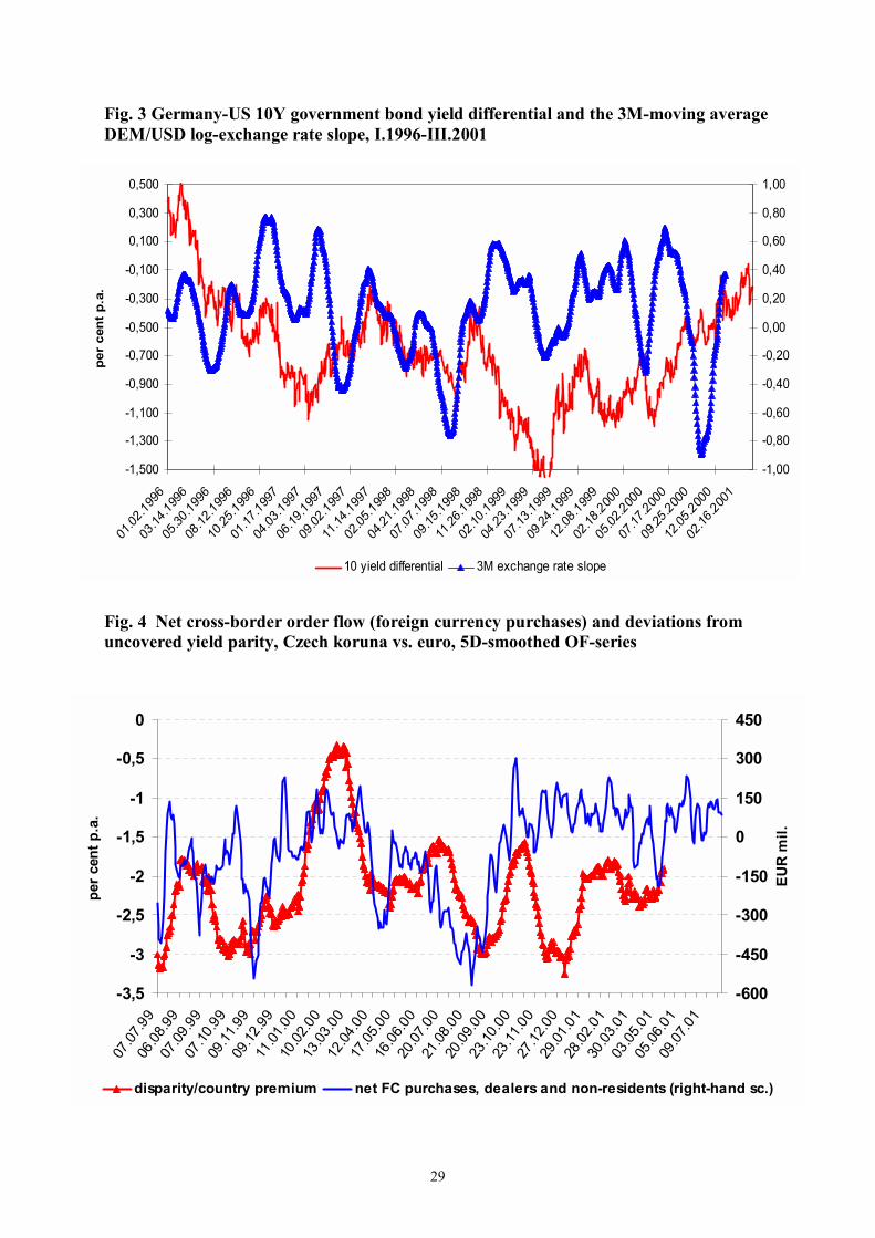
29

Fig. 3 Germany-US 10Y government bond yield differential and the 3M-moving average DEM/USD log-exchange rate slope, I.1996-III.2001 Fig. 4 Net cross-border order flow (foreign currency purchases) and deviations from uncovered yield parity, Czech koruna vs. euro, 5D-smoothed OF-series

-1,500

-1,300

-1,100

-0,900

-0,700

-0,500

-0,300

-0,100

0,100

0,300

0,500

01.02

.1996

03.14

.1996

05.30

.1996

08.12

.1996

10.25

.1996

01.17

.1997

04.03

.1997

06.19

.1997

09.02

.1997

11.14

.1997

02.05

.1998

04.21

.1998

07.07

.1998

09.15

.1998

11.26

.1998

02.10

.1999

04.23

.1999

07.13

.1999

09.24

.1999

12.08

.1999

02.18

.2000

05.02

.2000

07.17

.2000

09.25

.2000

12.05

.2000

02.16

.2001

per

cent

p.a

.

-1,00

-0,80

-0,60

-0,40

-0,20

0,00

0,20

0,40

0,60

0,80

1,00

10 yield differential 3M exchange rate slope

-3,5

-3

-2,5

-2

-1,5

-1

-0,5

0

07.07

.9906

.08.99

07.09

.9907

.10.99

09.11

.9909

.12.99

11.01

.0010

.02.00

13.03

.0012

.04.00

17.05

.0016

.06.00

20.07

.0021

.08.00

20.09

.0023

.10.00

23.11

.0027

.12.00

29.01

.0128

.02.01

30.03

.0103

.05.01

05.06

.0109

.07.01

per c

ent p

.a.

-600

-450

-300

-150

0

150

300

450

EUR

mil.

disparity/country premium net FC purchases, dealers and non-residents (right-hand sc.)