The Forward Premium Puzzle

in a Two-Country World

Ian Martin∗

March, 2013

Abstract

I explore the behavior of asset prices and the exchange rate in a two-country

world. When the large country has bad news, the relative price of the small

country’s output declines. As a result, the small country’s bonds are risky, and

uncovered interest parity fails, with positive excess returns available to investors

who borrow at the large country’s interest rate and lend at the small country’s

interest rate. I use a diagrammatic approach to derive these and other results

in a calibration-free way.

JEL code: G15.

∗ian.martin@gsb.stanford.edu; http://www.stanford.edu/∼iwrm/. First draft: April, 2010. I

am grateful to Fernando Alvarez, Dave Backus, Thomas Baranga, Jeremy Bulow, John Cochrane,

Darrell Duffie, Bernard Dumas, Lars Hansen, Tarek Hassan, Bruce Lehmann, Robert Lucas, Monika

Piazzesi, Roberto Rigobon, Martin Schneider, Andy Skrzypacz, Nancy Stokey, and Harald Uhlig,

and to seminar participants at Central European University, the University of Chicago Money &

Banking Workshop, the Stanford Institute for Theoretical Economics conference, Stanford GSB,

and UCSD for their comments.

1

An extensive literature has documented the fact that interest-rate differentials

across countries are not on average counteracted by offsetting currency movements.

As a result, it is possible to earn excess returns by investing in high-interest-rate

currencies and borrowing in low-interest-rate currencies. More specifically, Hassan

(2012) documents an empirical relationship between interest rates and country size:

smaller economies tend to have persistently higher interest rates, and the returns

on smaller economies’ bonds have higher covariances with long-run consumption

growth of US stockholders.

This paper presents a two-country model in which this failure of uncovered in-

terest parity (UIP)—also known as the forward premium puzzle—emerges in equi-

librium, and with this size-related pattern. The outputs of the two countries are

imperfect substitutes for one another, so units matter, and there are two term struc-

tures of interest rates, one for each good. Global financial markets are assumed to be

perfectly integrated; assets are real rather than nominal, and are priced by marginal

global investors with power utility; there are no non-tradable goods, no liquidity

issues, no portfolio constraints.

Even so, UIP fails to hold. Suppose, for example, that both countries have the

same distribution of output growth, and that one country is much smaller than

the other. In equilibrium, the smaller country has a higher short-term real interest

rate. But the small country’s exchange rate does not depreciate enough, on average,

to offset the interest-rate differential. In fact, on the contrary, the exchange rate

is expected to appreciate (in an example of Siegel’s (1972) “paradox”), thereby

increasing the expected excess return on the carry trade.

Why does the smaller country have a higher interest rate? Any risk-based ex-

planation must provide a story for why the small country’s bond underperforms

in bad states of the world. In the model considered here, the marginal investor

is particularly concerned with states in which the large country experiences low

output growth, since its output contributes the majority of the marginal investor’s

consumption. In such states, there is an increase in the relative supply of the small

country’s output, so its exchange rate depreciates, causing the small-country bond

to underperform; hence the risk premium.

These effects do not depend on finely tuned parameter values: UIP fails in any

calibration of the model, and I provide economically interpretable nonparametric

conditions under which I am able to sign the direction in which UIP fails—that

2

is, to show when it is the small country whose bonds are risky, as in the example

above. An unusual feature of the paper is that it develops a method of demonstrating

that this relationship holds via diagrammatic proofs. (More conventional, but less

comprehensible, algebraic proofs are provided in the supplementary appendix.) I

use this approach to show that various other relationships hold within the model,

for example between risk premia on the large and small countries’ output claims, in

own and foreign units.

Although the ingredients of the model are entirely standard, it has not previ-

ously been solved even in the lognormal case: the interactions between the model’s

additive features (a CES aggregator over multiple goods) and multiplicative features

(power utility and i.i.d. log consumption growth) that make it interesting also make

it hard to solve. These features capture the familiar tension in finance that portfolio

formation is additive while returns compound multiplicatively. The loglinearization

approach of Campbell and Shiller (1987) provides an approximate solution to this

problem. In the context of international finance, an alternative approach (adopted,

for example, by Cole and Obstfeld (1991), Zapatero (1995), Pavlova and Rigobon

(2007), and Stathopoulos (2009)) has been to focus on the knife-edge, but tractable

because multiplicative, Cobb-Douglas case of unit elasticity of substitution between

goods.

This paper avoids the need to loglinearize or to assume unit elasticity of sub-

stitution and provides an exact solution via Fourier transform methods, extending

Martin (2013b). Prices, interest rates and so on are expressed in terms of integral

formulas that allow for a range of specifications of output dynamics and can be

evaluated numerically almost instantly. They can also be solved analytically in the

limit in which one country becomes very small relative to the other, and this limit

turns out to capture many important features of the model in a highly tractable

setting. A further benefit is that it is possible to provide explicit conditions that

ensure that expected utility is finite; perhaps surprisingly, it does not appear to

be conventional to do so in the literature (Hansen and Scheinkman (2012) being a

notable exception).

Last but not least, the approach allows for jumps. Motivation for doing so is

provided by an increasingly large body of work that emphasizes the importance of

nonlognormality in financial markets (Rietz (1988), Barro (2006), Backus, Chernov,

and Martin (2011)); in particular, Martin (2011) shows that no conditionally log-

3

normal model is consistent with index option prices in the US. Jumps also enable

the model to replicate the finding that carry trade returns are negatively skewed

(Brunnermeier, Nagel and Pedersen (2008), Jurek (2009)) and to generate sensible

risk premia without implausibly high risk aversion. The key to retaining tractabil-

ity in the presence of jumps is the cumulant-generating function (CGF), which was

also exploited in Martin (2013b). This paper introduces some new properties that

CGFs may or may not possess, and which provide nonparametric ways of restricting

possible calibrations. For example, in a lognormal world one might want to assume

that countries have linked fundamentals in the sense of having (weakly) positively

correlated log output growth. A contribution of the paper is to identify—for this

example and others—the right definition that generalizes beyond the lognormal case.

A final benefit of allowing for jumps is that the results hold independently of

Merton’s (1973) ICAPM and Breeden’s (1979) consumption-CAPM, which do not

hold once asset prices can jump; this is reassuring, given the mixed empirical per-

formance of the ICAPM and consumption-CAPM.

When not included in the body of the paper, proofs are in the appendix.

Related literature. Frankel (1980), Hansen and Hodrick (1980), and Fama (1984)

are amongst the early contributions to the literature on the forward premium puzzle.

More generally, Dumas, Harvey and Ruiz (2003) present evidence that international

markets are well integrated; Lustig, Roussanov and Verdelhan (2009) provide sup-

port for the idea that the behavior of international asset prices is amenable to a

risk-based explanation; and Hollifield and Yaron (2003) argue that models of cur-

rency risk premia should focus on real, as opposed to nominal, risk. Alvarez, Atkeson

and Kehoe (2007) emphasize that the empirical fact that exchange rates are approx-

imately random walks implies that fluctuations in interest rates are associated (in

their lognormal setting) with changes in conditional variances of the log SDF. This

is a feature of the model presented below.1

Hassan (2012) motivates his empirical results with a two-period, lognormal and

loglinearized model with one tradable good and multiple non-tradable goods, un-

der an assumption that a transfer before the start of period 1 equates all agents’

1Of the theoretical papers mentioned in this introduction, Alvarez, Atkeson and Kehoe (2007),

Cochrane, Longstaff and Santa-Clara (2008), Colacito and Croce (2010), Hassan (2012), Lustig,

Roussanov and Verdelhan (2009), Pavlova and Rigobon (2007), Stathopoulos (2009), Verdelhan

(2009), and Zapatero (1995) impose conditional lognormality.

4

wealth. Verdelhan (2010) considers a model with habit formation. Colacito and

Croce (2010) and Bansal and Shaliastovich (2010) argue that long-run risk, to-

gether with Epstein-Zin preferences, can explain the forward premium puzzle. Farhi,

Fraiberger, Gabaix, Ranciere and Verdelhan (2009) construct a model featuring rare

disasters, and present supporting evidence from FX option data.

Piazzesi, Schneider and Tuzel (2007) present a model with housing and non-

housing goods that are imperfect substitutes for one another. Their stochastic

discount factor takes the same form as that of the present paper, but the driving

stochastic processes are modelled differently so that their analog of my state variable

u mean-reverts rather than following a Levy process.

To my knowledge, no other paper in this literature derives calibration-free results

of the type presented here.

1 UIP and the forward premium puzzle

UIP is a conjectured relationship between next year’s spot exchange rate between

two countries, et+1, today’s spot exchange rate, et, and 1-year interest rates in each

country, i1,t and i2,t:

Et log et+1?= log et + i1,t − i2,t . (1)

The thought behind (1) is this: if country 2 has a lower interest rate than country

1, surely this should be compensated by the expected appreciation of its currency?

Unfortunately this plausible idea is decisively rejected by the data: in the relation-

ship

log et+1 − log et = a0 + a1(i1,t − i2,t) + εt+1 , (2)

UIP holds if a0 = 0 and a1 = 1. But typical estimates place a1 close to (and often

less than) zero.

An equivalent formulation of UIP exploits covered interest parity, which is the

no-arbitrage—and therefore robust—relationship between today’s 1-year forward

exchange rate, ft, today’s spot exchange rate, and the two countries’ 1-year rates:

log ft = log et + i1,t − i2,t. Using this relationship, equation (1) can be expressed as

Et log et+1 = log ft, so the failure of UIP is equivalent to the fact that log forward

rates are biased predictors of future log exchange rates.

If we write Mi,t+1 for the stochastic discount factor (SDF) that prices assets

whose payoffs are in units of country i’s good, then (as we will see below) the

5

relationship et+1/et = M2,t+1/M1,t+1 holds. Taking logs then expectations we have

the identity

Et ∆ log et+1 = Et logM2,t+1 − Et logM1,t+1 . (3)

Now, if M1,t+1 and M2,t+1 were roughly constant—as would be the case if either

there were little risk in the economy, or if investors were roughly risk-neutral—then

we could approximate (3) by

Et ∆ log et+1 ≈ logEtM2,t+1 − logEtM1,t+1 = i1,t − i2,t . (4)

That is, UIP would approximately hold in economies in which either the price or

quantity of risk was very low. Empirically, however, the fact that high Sharpe ratios

are attainable tells us, thanks to the Hansen-Jagannathan (1991) bound, that the

SDFs Mi,t+1 are volatile. Thus the move from (3) to (4) was not justified, and we

must take the effects of Jensen’s inequality into account, arriving at the identity

Et ∆ log et+1 = i1,t−i2,t+logEtM1,t+1 − Et logM1,t+1︸ ︷︷ ︸Lt(M1,t+1)

− (logEtM2,t+1 − Et logM2,t+1)︸ ︷︷ ︸Lt(M2,t+1)

.

(5)

The terms Lt(Mi,t+1) measure SDF variability; I call Lt(Mi,t+1) the entropy of

Mi,t+1, following Backus, Chernov and Martin (2011). High attainable expected log

returns translate into high SDF entropy (Bansal and Lehmann (1997), Alvarez and

Jermann (2005)), much as high attainable Sharpe ratios translate into high SDF

volatility.

The identity (5) reveals some necessary ingredients of any model in which UIP

fails to hold (see also Fama (1984), and Backus, Foresi and Telmer (2001)). First,

as discussed, the entropies of M1,t+1 and M2,t+1 must be non-zero and economically

significant: risk must matter. Second, there must be an asymmetry: if the entropies

were equal they would cancel out, returning us to a world in which UIP held. Third,

to generate the patterns found when estimating (2), Lt(M1,t+1)−Lt(M2,t+1) should

be small at times when i1,t−i2,t is high: assets denominated in the high-interest-rate

currency should have relatively low risk-adjusted returns. The model that follows

has these properties.

6

2 The model

There are two countries with output streams {D1t} and {D2t} respectively, at least

one of which is nondeterministic. There are three classes of agents. The first two

classes are made up of locals in each country; these are hand-to-mouth consumers

who, in aggregate, consume a fraction 1 − φ of their own country’s output and do

not eat the foreign country’s output. The third class comprises the jetsetters: these

individuals eat goods from both countries, consuming the remaining fraction φ of

each country’s output. (One could embed this structure in a model in which output

is produced as a Cobb-Douglas function of capital, owned by jetsetters, and labor,

owned by locals.) The goods are viewed as imperfect substitutes by jetsetters, and

η ∈ [1,∞) is the elasticity of intratemporal substitution between goods 1 and 2.

Locals do not participate in financial markets, so assets are priced by the jetsetters,

each of whose expected utility takes the form (up to the irrelevant constant multiple

φ1−γ)

E∫ ∞0

e−ρtC1−γt

1− γdt , where Ct ≡

[w1/ηD

η−1η

1t + (1− w)1/ηDη−1η

2t

] ηη−1

.

The constant w controls the relative importance of goods 1 and 2 for jetsetters.

These assumptions implicitly embed the view that financial markets are well

integrated, since the jetsetters are the marginal agents pricing both countries’ output

claims and riskless bonds; as a result, asset prices will be more highly correlated

across countries than outputs, and shocks will be transmitted from one market

to another. On the other hand, the model is also consistent with the view that

aggregate consumption risk is imperfectly shared across countries (Backus, Kehoe

and Kydland (1992)) due to the presence of the locals who do not participate in

asset markets. Nonparticipation is a feature of the data: Calvet, Campbell and

Sodini (2007) analyze a comprehensive dataset that covers all Swedish households

and report that 38 per cent of households were nonparticipants.

Write v(D1t, D2t) ≡ C1−γt /(1−γ) for the instantaneous felicity function, vi(D1t, D2t)

for the marginal utility of good i, et ≡ v2(D1t, D2t)/v1(D1t, D2t) for the intratempo-

ral price of a unit of good 2 in units of good 1, andMiτ ≡ e−ρ(τ−t)vi(D1τ , D2τ )/vi(D1t, D2t)

for the SDF that prices time-τ claims to good i. The SDFs M1τ and M2τ and the

relative price et are related, as noted above, by the equation

eτet

=M2τ

M1τ,

7

which appears as Proposition 1 of Backus, Foresi and Telmer (2001) and as equation

1 of Brandt, Cochrane and Santa-Clara (2006). I refer to the relative price et as the

exchange rate, because it is the relative price of locals’ consumption baskets in the

two countries. When the relative supply of country 2’s good declines, the exchange

rate et increases.2

The price at time t of asset i is given by Lucas’s (1978) Euler equation

Pit = E∫ ∞t

MiτDiτ dτ . (6)

Similarly, the price (in own units) of a perpetuity that pays out a constant stream

of good i dividends at a rate of one per unit time, is given by (6) with Diτ replaced

by 1.

It is important to emphasize, first, that we need two different SDFs because

there are two different types of assets, with payouts denominated in two different

goods and, second, that the perturbation logic underlying (6) implies that the price

Pit is denominated in units of good i (“in i-units”). I use stars to indicate a price

not expressed in its own units: P ∗2t = P2tet and P ∗1t = P1t/et.

The outputs of the two countries, D1t and D2t, are taken as exogenous—though

they could also be thought of as being determined by a production side of the

economy that is left unmodelled here—and are assumed to have dividend growth

that is i.i.d. over time, though not necessarily across countries. Formally, yit−yi0 ≡logDit − logDi0 is a Levy process for i = 1, 2.

Definition 1. The cumulant-generating function (CGF) c(θ1, θ2) is defined by

c(θ1, θ2) ≡ logE eθ1(y1,t+1−y1,t)+θ2(y2,t+1−y2,t) = logE

[(D1,t+1

D1,t

)θ1 (D2,t+1

D2,t

)θ2].

The CGF captures all relevant information about the technological side of the

model. Mean log output growth of country j is ∂c∂θj

(0, 0), the variance of log output

2The model does not address the finding of Backus and Smith (1993) that there is considerable

variation in exchange rates that is not explained by variation in relative consumption. Stockman

and Tesar (1995) suggest that this shortcoming can be addressed by introducing taste shocks. In

the present setup we can do so by allowing the weights w and 1−w in the consumption aggregator

to follow exponential Levy processes. This extension comes at the cost of an increase in complexity,

however, and the goal of this paper is to demonstrate that the failure of UIP emerges robustly in

a simple model.

8

growth of country j is ∂2c∂θ2j

(0, 0), and the covariance between the log output growth

of countries j and k is ∂2c∂θj∂θk

(0, 0). Third-order and higher partial derivatives at

the origin capture higher cumulants and co-cumulants of output growth: skewness,

excess kurtosis, and so on.

By exploiting general properties of CGFs, it is possible to establish features

of asset prices in this economy that hold not just for a particular calibration but

for a whole family of driving stochastic processes. The most important such prop-

erty is that CGFs are always convex. But I also find it helpful to introduce three

nonparametric properties, each of which the CGF may or may not possess. The

first is the exchangeability property,3 which holds if c(θ1, θ2) = c(θ2, θ1). This is a

cet. par. assumption: it ensures the two countries have the same means and volatil-

ities of output growth, the same arrival rates of jumps, and so on. It therefore

focusses attention on the underlying economic mechanism and on the consequences

of asymmetry in country size alone. The second is the convex difference property,

which is a restriction on the higher cumulants of log output growth. It holds in

the lognormal case, and more generally it ensures, roughly speaking, that output

growth in each country is not positively skewed. The third is the linked fundamentals

property. In the lognormal case, it is natural to consider imposing the economically

plausible assumption that the correlation between the two countries’ output growth

is nonnegative. The linked fundamentals property, which will turn out to be the

appropriate generalization for arbitrary Levy processes, requires that the CGF is

supermodular.

It may be helpful to consider some parametric examples of CGFs. Write θ ≡(θ1, θ2)

′ and yt ≡ (y1t, y2t)′.

(i) If output growth is lognormal, i.e. yt = y0 + µt + AZt, where µ is a 2-

dimensional vector of drifts, A a 2 × 2 matrix of factor loadings, and Zt a

2-dimensional Brownian motion, then the CGF is

c(θ1, θ2) = µ′θ + θ′Σθ/2, (7)

where Σ ≡ AA′ is the covariance matrix of log output growth, whose elements

I write as σjk. If the countries have independent output growth then Σ is a

3Two random variables X1, X2 are exchangeable if the distribution of (X1, X2) is the same as

that of (X2, X1).

9

diagonal matrix, so the CGF decomposes as c(θ1, θ2) = c1(θ1) + c2(θ2) where

ck(θk) ≡ µkθk + σkkθ2k/2.

(ii) If log dividends follow a jump-diffusion, we can write yt = y0 + µt +AZt +∑K(t)k=1 J

k, where K(t) is a Poisson process with arrival rate ω that represents

the number of jumps that have taken place by time t, and Jk are 2-dimensional

random variables that are i.i.d. across k. There may be arbitrary correlations

between the elements of J . (I will write J ≡ J1 when I discuss the distri-

bution of these random variables.) The CGF then acquires an extra term,

whose precise nature depends on the assumptions made about the jump size

distribution: c(θ1, θ2) = µ′θ + θ′Σθ/2 + ω(E eθ′J − 1

).

(iii) By specifying the jump distribution J appropriately, this framework allows for

multiple types of jump. Letting p1, p2, and p3 be probabilities summing to one,

suppose that with probability p1, J shocks the log output of country 1 by a

Normal random variable with mean µ(1)1 and variance σ

(1)11 ; with probability p2,

J shocks the log output of country 2 by a Normal random variable with mean

µ(2)2 and variance σ

(2)22 ; and with probability p3, J shocks both log outputs

simultaneously by a bivariate Normal random variable with mean (µ(3)1 , µ

(3)2 )′

and covariance matrix

(σ(3)11 σ

(3)12

σ(3)12 σ

(3)22

). This is a special case of Example (ii), so

the CGF is

c(θ1, θ2) = µ1θ1 + µ2θ2 +1

2σ11θ

21 + σ12θ1θ2 +

1

2σ22θ

22 + ω1

(eµ

(1)1 θ1+

12σ(1)11 θ

21 − 1

)+

+ ω2

(eµ

(2)2 θ2+

12σ(2)22 θ

22 − 1

)+ ω3

(eµ

(3)1 θ1+µ

(3)2 θ2+

12σ(3)11 θ

21+σ

(3)12 θ1θ2+

12σ(3)22 θ

22 − 1

),

where ωk = ωpk for k = 1, 2, 3.

(iv) Specializing still further, suppose that output is i.i.d. across countries. Inde-

pendence requires that σ12 = ω3 = 0, and identical distribution means that we

can simplify the notation by writing µk = µ, σkk = σ2, µ(k)k = µJ , σ

(k)kk = σ2J ,

and finally ω1 = ω2 = ω for the arrival rate of each country’s jumps. The

CGF is then

c(θ1, θ2) = µθ1+µθ2+1

2σ2θ21+

1

2σ2θ22+ω

(eµJθ1+

12σ2Jθ

21 − 1

)+ω

(eµJθ2+

12σ2Jθ

22 − 1

).

(8)

The symmetry of the two countries is reflected in the fact that exchangeability

holds in (8), i.e. c(θ1, θ2) = c(θ2, θ1). Their independence is reflected in the

10

fact that the CGF can be decomposed as a function of θ1 plus a function of

θ2 (so for example there are no cross-terms θ1θ2).

For the purposes of illustration (only), I consider a calibration in which output

growth is i.i.d. across countries so that any correlations or asymmetries that emerge

do so endogenously; the associated CGF is given by (8). I assume that log output in

each country has a Brownian motion component with drift µ = 0.02 and volatility

σ = 0.1. Each country is also afflicted by jumps, which arrive at times dictated by

a Poisson process with arrival rate ω = 0.02. When a country experiences a jump,

the shock to its log output is Normal with mean µJ = −0.2 and volatility σJ = 0.1.

I also assume that the marginal investor has time preference rate ρ = 0.04 and

risk aversion γ = 4; that the weight of country 1 in the consumption aggregator is

w = 0.2; and that the elasticity of substitution between goods is η = 2.

For the general results, I assume that γη ≥ 2; typical estimates in the literature

put both γ and η somewhere in the range 2–10, so this is a mild assumption. It will

be convenient to write χ = (η− 1)/η and γ = (γ + χ− 1)/χ. The variable χ ranges

between 0 (the Cobb-Douglas case) and 1 (the perfect substitutes case). Result 6

requires the further assumption that γ is an integer.

Given the specification of tastes and technology—specifically, given that prefer-

ences are power utility over a CES aggregator and log outputs follow Levy processes—

price-dividend ratios, interest rates and expected returns are invariant to scalings

(D1t, D2t) 7→ (kD1t, kD2t). These quantities do however depend on a single state

variable that indexes the relative sizes of the two countries. In principle this state

variable could be any monotonic function of D2t/D1t, but it will be most convenient

to work with

ut ≡ (1− χ) log1− ww

+ χ logD2t

D1t= (1− χ) log

1− ww

+ χ(y2t − y1t).

The state variable ut is a Levy process because y1t and y2t are Levy processes. The

constant term (1 − χ) log[(1 − w)/w] ensures that ut = 0 if countries 1 and 2 have

equal shares of world output. I plot graphs against the alternative state variable

st ≡ 1/(1 + eut). This is less mathematically convenient than ut because it is not a

Levy process, but it has a nice interpretation as country 1’s share of world output,

st =D1t

D1t + et ·D2t.

11

Before jumping into the solution of the model, it may be helpful to explore one

of its most important components. If we define the marginal investor’s risk aversion

to a good-i shock as γi ≡ −Divii/vi, some algebra shows that

γ1 =1

η+

(γ − 1

η

)st (9)

and, symmetrically, that risk aversion to a good-2 shock is γ2 = 1/η+(γ−1/η)(1−st).Thus the marginal investor’s attitude to the risk associated with a country’s output

depends on the size of that country. As country 1’s share of world output, st,

declines from 1 to 0, risk aversion to good-1 shocks declines linearly from γ to 1/η.

Equation (9) also provides a way to understand the models of Cochrane, Longstaff

and Santa-Clara (2008) and of Martin (2013b)—but in those models η =∞, so that

when country 1 is negligibly small the marginal investor is risk-neutral to good-1

shocks. Here, with η < ∞, the agent remains averse to the risk of good 1 even if

country 1 is very small because good 2 is only an imperfect substitute for it. This

effect will drive up risk premia on a small country’s output claim relative to the

η =∞ case.

2.1 Prices

The first result characterizes the behavior of the exchange rate in terms of the

driving output processes. The proof exploits the following useful, and completely

general, property of CGFs.

Property 0 (Convexity). Any cumulant-generating function c(θ1, θ2) is convex.

The convexity property makes it possible to prove results that are valid for

dividends driven by any Levy process with finite moments. This property is used

in the result below, in a rather simple form, to show that Siegel’s (1972) “paradox”

holds, and will be used in more complicated situations in subsequent results. Since

the convexity logic will be used throughout the paper, I illustrate its application in

Figure 1.

Result 1 (Exchange rate). The exchange rate et is

et = [(1− w)/w]1/η(D2t/D1t)−1/η

= [(1− w)/w](1−χ)/χ · exp {−[(1− χ)/χ]ut} . (10)

12

This means that the log exchange rate is a Levy process.

The expected appreciation in country 1’s exchange rate, FX∗1 , is

FX∗1 dt ≡E d(1/et)

1/et= c(χ− 1, 1− χ) dt, (11)

and the expected appreciation in country 2’s exchange rate, FX∗2 , is

FX∗2 dt ≡E detet

= c(1− χ, χ− 1) dt. (12)

If η < ∞, so that exchange rates are nonconstant, then the average expected

appreciation, (FX∗1 + FX∗2 )/2, is positive—an instance of Siegel’s paradox.

Proof. Equation (10) follows from the fact that et = v2(D1t, D2t)/v1(D1t, D2t) and

the definition of the state variable ut. For arbitrary constants w1 and w2,

E [d (ew1y1t+w2y2t)]

ew1y1t+w2y2t= c(w1, w2) dt . (13)

Equations (11) and (12) follow by applying (13) to equation (10).

It remains to show that Siegel’s paradox holds, i.e. that c(χ− 1, 1− χ) + c(1−χ, χ − 1) > 0. If dividend growth is lognormal, so that the CGF is given by (7),

then we must show that (1− χ)2(σ11 − 2σ12 + σ22) > 0. The first factor, (1− χ)2,

is positive if η < ∞ since then χ < 1, and the second factor is positive because it

equals the variance of (y1,t+1 − y1,t)− (y2,t+1 − y2,t). This establishes the result for

the lognormal case.

Property 0 provides exactly the right line of attack to prove the result in the

general case. Since c(0, 0) = 0 for any CGF, the goal is to show that c(χ−1, 1−χ)−2c(0, 0)+c(1−χ, χ−1) is positive. Figure 1a plots the convex surface parametrized

by (θ1, θ2, c(θ1, θ2)). The points (χ − 1, 1 − χ, c(χ − 1, 1 − χ)) and (1 − χ, χ −1, c(1 − χ, χ − 1)) lie on this surface and are indicated with plus signs; the point

(0, 0, c(0, 0))—i.e., the origin, since c(0, 0) = 0—is correspondingly indicated with

(two, overlapping) minus signs. It is now clear that, by convexity, c(χ− 1, 1− χ)−2c(0, 0) + c(1−χ, χ− 1) is positive, as shown in Figure 1a. For comparison, Figure

1c illustrates the fact that c(0,−γ)+c(−γ, 0)−c(χ−1, 1−χ−γ)−c(1−χ−γ, χ−1)

is positive, which will be useful in Result 8, below.

Convexity arguments, as employed in the above proof, will be useful throughout

the paper. Figures 1b and 1d therefore represent the information in Figures 1a and

13

(a) c(χ−1, 1−χ)−2c(0, 0)+c(1−χ, χ−1) > 0

Χ-1 1- ΧΘ1

Χ-1

1- Χ

Θ2

Å

Å

2�

(b) A simpler representation of panel (a)

(c) c(0,−γ) + c(−γ, 0)− c(χ− 1, 1−χ− γ)−c(1− χ− γ, χ− 1) > 0

Χ-1-Γ 1- Χ-ΓΘ1

Χ-1

-Γ

1- Χ-Γ

Θ2

Å

Å

�

�

(d) A simpler representation of panel (c)

Figure 1: Exploiting CGF convexity. Panels (a) and (b) illustrate Siegel’s paradox.

1c in a more convenient way, so that it is immediately obvious if an expression is

positive by virtue of convexity: we require the four points—counted with multiplic-

ity, so that the origin in Figures 1a and 1b counts as two points—to be arranged

on any straight line in (θ1, θ2)-space, symmetrically about their midpoint, and with

sign pattern as in Figures 1b and 1d.

Figure 2a shows how the exchange rate varies as a function of country 1’s output

share in the calibration described in the previous section. When country 1 is small,

14

0.2 0.4 0.6 0.8 1.0s

0.1

1

10

100

(a) et

0.2 0.4 0.6 0.8 1.0s

20

40

60

80

100P1�D1

(b) P1/D1

Figure 2: Left: The exchange rate—the relative price of good 2 in units of good

1—plotted against s, the output share of country 1. Right: Price-dividend ratio on

asset 1, plotted against s, in the imperfect substitution case η = 2 (black) and the

perfect substitution case (dashed red).

its goods are in short supply so command a high price. (In the perfect-substitutes

case the relative price would always equal 1, independent of country 1’s output

share.) Since the weight of country 1 in the consumption aggregator is w = 0.2, the

exchange rate et equals 1 when s = 0.2.

The next result provides integral formulas for the price-dividend ratios of the

two countries’ output claims and for the prices of each country’s perpetuity—where,

within the model, country i’s perpetuity is a security that delivers one unit of good

i per unit of time. In the case with no jumps these integrals can be expressed in

closed form in terms of hypergeometric functions, as in Martin (2013b). I do not

pursue this approach here because the integral formulas apply more generally and

can be numerically evaluated almost instantaneously.

Result 2 (Valuation ratios). The price-dividend ratios, Pit/Dit, of each country’s

output claim, and the prices of each country’s perpetuity, Bit, i = 1, 2, are

P1t/D1t = V1,0(ut)

P2t/D2t = V0,1(ut)

B1t = V1−1/χ,0(ut) (14)

B2t = V0,1−1/χ(ut), (15)

15

where

Vα1,α2(u) ≡(eu/2 + e−u/2

)γ ∫ ∞−∞

eiuzF (z)

ρ− c[χ(α1 − γ/2− iz), χ(α2 − γ/2 + iz)]dz

and F (z) ≡ 12π · Γ(γ/2− iz)Γ(γ/2 + iz)/Γ(γ).

The proof of Result 2 shows that we need some assumptions to guarantee that

asset prices and expected utility are well defined. Specifically, the discount rate, ρ,

must be high enough that ρ− c [χ(α1 − γ/2), χ(α2 − γ/2)] > 0 for a range of values

of α1 and α2: namely, α1 = 1, α2 = 0, so that the output claim of country 1 has

a finite price; α1 = 0, α2 = 1, so that the output claim of country 2 has a finite

price; α1 = 1 − 1/χ, α2 = 0, so that country 1’s perpetuity has a finite price; and

α1 = 0, α2 = 1 − 1/χ, so that country 2’s perpetuity has a finite price. The first

two of these assumptions—all of which are summarized in Table 1, after rewriting

γ and χ in terms of γ and η—ensure that expected utility is finite.

Restriction Reason

ρ− c(1− γ/2− 1/(2η),−γ/2 + 1/(2η)) > 0 finite price of asset 1

ρ− c(−γ/2 + 1/(2η), 1− γ/2− 1/(2η)) > 0 finite price of asset 2

ρ− c(−γ/2− 1/(2η),−γ/2 + 1/(2η)) > 0 finite price of perpetuity 1

ρ− c(−γ/2 + 1/(2η),−γ/2− 1/(2η)) > 0 finite price of perpetuity 2

Table 1: The restrictions imposed on the model.

Valuation ratios move around over time as dividends, and hence ut and st, move

around. Figure 2b plots the price-dividend ratio of the claim to country 1’s output

stream, P1/D1, against country 1’s output share, s. The solid line is the price-

dividend ratio in the imperfect substitution case, using the same calibration as

above, and the dashed line shows the price-dividend ratio in the perfect substitutes

case. The price-dividend ratio increases sharply as country 1’s share of output

declines in both the perfect and imperfect substitution cases, though the effect is

muted in the latter case.

Figure 3 shows an illustrative sample realization over a two-year period. Panel

3a plots the paths of exogenous fundamentals: the outputs, or dividends, produced

by the two countries. The larger country (black line) initially contributes 80% of

global output. After about 0.6 years, it experiences a disaster that causes its output

to drop; the smaller country experiences a similar disaster after about 1.5 years.

16

0.5 1.0 1.5 2.0

1

2

3

4

(a) Dividends

0.0 0.5 1.0 1.5 2.0

50

20

30

15

(b) Bond prices in large coun-

try’s currency, η = 1

0.0 0.5 1.0 1.5 2.0

50

20

30

15

(c) Bond prices in large coun-

try’s currency, η = 2

0.0 0.5 1.0 1.5 2.0

50

20

30

15

(d) Bond prices in large coun-

try’s currency, η =∞

0.0 0.5 1.0 1.5 2.0

50

20

30

15

(e) Bond prices in small coun-

try’s currency, η = 1

0.0 0.5 1.0 1.5 2.0

50

20

30

15

(f) Bond prices in small coun-

try’s currency, η = 2

0.0 0.5 1.0 1.5 2.0

50

20

30

15

(g) Bond prices in small coun-

try’s currency, η =∞

Figure 3: Prices, in each currency, of the large country’s perpetuity (black) and

small country’s perpetuity (red) along a particular sample path, for different values

of the elasticity of substitution between goods, η. Each figure is plotted on a log

scale, and is based on the same underlying path of fundamentals, shown in panel

(a).

17

The panels below show how the behavior of perpetuity prices, given by (14)

and (15), depends on the elasticity of substitution between goods, η, with the large

country’s bond in black and the small country’s bond in red. The left-hand column

sets η = 1, so that consumption is a Cobb-Douglas aggregator of the two goods.

Panels 3b and 3e illustrate the distinctive feature of the Cobb-Douglas setup that

bond prices are constant in their own currency, despite the large shocks each country

experiences. On the other hand, the exchange rate is extremely volatile, so for exam-

ple the price of the large country’s bond, denominated in the small country’s units,

jumps up when the large country experiences its output disaster. The right-hand

column shows the other extreme, in which the two goods are perfect substitutes.

The exchange rate effect disappears: panels 3d and 3g show that bond prices in

the perfect substitutes case are the same in each set of units. Put crudely, in the

Cobb-Douglas case all the action is in exchange rates and none in valuation ratios,

in conflict with the overwhelming empirical evidence that movements in valuation

ratios are a major driver of asset returns;4 and in the perfect substitutes case all

the action is in valuation ratios and none in exchange rates.

In between, both effects are present. Panel 3c shows that in large country units,

exchange rate movements exacerbate the poor performance of the small country’s

bond when the large country suffers its disaster. As a result, the small bond is

riskier than the large bond, and so the overall level of the small bond’s price is lower,

reflecting higher interest rates in the small country and hence the emergence of a

carry trade. Notice, also, that the carry trade experiences severe underperformance

at times of large-country disaster. Panel 3f shows the corresponding plots viewed

in small country units. The large country’s disaster reduces the relative supply of

its good, so its currency appreciates. In small-country units, the large country’s

bond therefore outperforms at the time of disaster and hence is a hedge, so earns a

negative excess return.

The price-dividend ratio of each country’s output claim also depends on the

relative size of the two economies, as in Cochrane, Longstaff and Santa-Clara (2008)

and Martin (2013b). If, say, the large country experiences bad output news then

the small country’s output share increases; its output claim is now riskier—more

correlated with consumption growth—so requires a higher excess return and a lower

price-dividend ratio. Thus shocks to one country affect asset valuations in the other

4See Cochrane (2008) for a recent survey.

18

country. Furthermore, if goods are imperfect substitutes, then the small country’s

currency depreciates when the large country experiences bad output news, as before.

This amplifies the underperformance of the small-country output claim in large-

country units. I illustrate this in the supplementary appendix, using the same

output sample paths as in Figure 3.

2.2 Interest rates

To understand why valuation ratios behave as they do, we must turn to the be-

havior of interest rates and risk premia. Each good has its own set of zero-coupon

bond prices, and attached to these bond prices are zero-coupon yields that move

around over time as shocks to the outputs of the two countries induce changes in u.

Three measures of interest rates are particularly natural: the riskless rates for each

good, calculated from zero-coupon yields in the limit as T → 0; coupon yields on

perpetuities, 1/BiT , provided by equations (14) and (15), which can be viewed as

a weighted average of yields of all maturities; and long rates, which are calculated

from zero-coupon yields as T →∞.

Result 3 (Interest rates). Writing YT,i(u) for the continuously compounded T -

period zero-coupon yield in i-units when the current state is u, we have

YT,1(u) =−1

Tlog

{(eu/2 + e−u/2

)γ ∫ ∞−∞

eiuzF (z)e−{ρ−c[χ(1−1/χ−γ/2−iz),χ(−γ/2+iz)]}T dz

}YT,2(u) =

−1

Tlog

{(eu/2 + e−u/2

)γ ∫ ∞−∞

eiuzF (z)e−{ρ−c[χ(−γ/2−iz),χ(1−1/χ−γ/2+iz)]}T dz

}.

The riskless rates, Rf,i(u) = limT→0 YT,i(u), i = 1, 2, are

Rf,1(u) =(eu/2 + e−u/2

)γ ∫ ∞−∞

eiuzF (z) {ρ− c[χ(1− 1/χ− γ/2− iz), χ(−γ/2 + iz)]} dz

Rf,2(u) =(eu/2 + e−u/2

)γ ∫ ∞−∞

eiuzF (z) {ρ− c[χ(−γ/2− iz), χ(1− 1/χ− γ/2 + iz)]} dz.

In this notation, the currently prevailing one-year rate in country j, as discussed

in Section 1, is ij,t = Y1,j(u). In contrast to short rates, we will now see that long

rates are always constant over time, and often constant across countries too.

19

Result 4 (The behavior of long interest rates). Long rates, Y∞,i ≡ limT→∞YT,i(u),

are independent of u, hence constant over time:

Y∞,1 = maxθ∈[0,γ+χ−1]

ρ− c(θ − γ,−θ) (16)

Y∞,2 = maxθ∈[0,γ+χ−1]

ρ− c(−θ, θ − γ) . (17)

When the exchangeability property holds, Y∞,1 = Y∞,2 = ρ − c(−γ/2,−γ/2), so

long rates are independent of the elasticity of substitution between goods. Even if

exchangeability does not hold, long rates are equated across countries whenever the

maximum in (16) is attained for θ ∈ (1− χ, γ + χ− 1).

Given the result of Dybvig, Ingersoll and Ross (1996), it is not particularly

surprising that long rates are constant across time. But it is interesting, and non-

obvious, that under mild conditions long rates should be constant across countries,

and should be independent of the substitutability of their outputs. For a given

CGF, it is easy to specify these “mild conditions” precisely by checking the condition

provided in the last sentence of Result 4 explicitly. More generally, long rates will be

equated if the countries’ output growth processes have sufficiently similar moments

and their goods are sufficiently good substitutes.

Figure 4a shows how the riskless rate (black solid line), perpetuity yield (red

dashed line), and long rate (blue dotted line) depend on s. Riskless rates are low

when s is close to 0 or to 1 due to precautionary savings demand in the face of an

unbalanced—because poorly technologically diversified—economy, and high when s

is close to 0.5. Country 1’s yield curve can be upward-sloping, downward-sloping,

or hump-shaped.

The figure is not symmetric: country 1’s interest rate is higher when it is small

than when it is large. In this example, as country 1’s share of global output declines

to zero, its interest rate approaches 3.25% while the large country’s interest rate

drops to 1.18%. From the perspective of an investor (or economist) thinking in

large country units, this might suggest the following carry trade: borrow at the

large-country interest rate of 1.18%, and invest in the small-country interest rate of

3.25%. We have not yet taken into account the effects of exchange-rate movements,

however. Before doing so, recall that in this example the exchangeability property

holds:

Property 1 (Exchangeability). c(θ1, θ2) = c(θ2, θ1) for all θ1, θ2.

20

0.2 0.4 0.6 0.8 1.0s

0.01

0.02

0.03

0.04

0.05

0.06

(a) Interest rates plotted against output

share

1 2 3 4t

0.96

0.98

1.00

1.02

1.04

(b) Forward and expected spot exchange

rates

Figure 4: Left: Country 1’s riskless rate (black solid), perpetuity yield (red dashed),

and long rate (blue dotted). Right: Forward price to time t of good 2 in 1-units

(F0→t, black solid), expected future spot prices (E et = E 1/et, red dashed), and

forward price of good 1 in 2-units (1/F0→t, blue dotted), plotted against t, assuming

starting share s = w = 20%.

From Result 1, we know that (FX∗1 +FX∗2 )/2, is positive. But the exchangeabil-

ity property and equations (11) and (12) imply that FX∗1 = FX∗2 , so it follows that

both are strictly positive. Thus exchange rate movements actually work in favor of

the carry trade. The reason for the carry trade’s excess return is (of course) that

it is risky: if the large country has bad news, the small country’s exchange rate

deteriorates, and the carry trade has a low return.

Returning to the general case, we can now see how the model generates the

failure of uncovered interest parity in the regression (2). We saw in Result 1 that

log et is a Levy process, so log et+1 − log et is independent of information known at

time t, and in particular of i1,t and i2,t. Thus cov(log et+1 − log et, i1,t − i2,t) = 0;

combining this with the fact that var(i1,t − i2,t) 6= 0, we have

Result 5 (Failure of UIP). Interest-rate differentials are totally uninformative about

future movements of the exchange rate: plim(a1) = 0.

Given that the random walk nature of log et+1 − log et was hard-wired in, the

interesting aspect of the model is not that it generates cov(log et+1 − log et, i1,t −i2,t) = 0 but that interest rates vary across countries, var(i1,t− i2,t) 6= 0, despite the

random walk character of exchange rates.

The failure of UIP can also be recast in terms of forward rates. Let F0→t be

21

the time-0 forward price of good 2 in 1-units, for settlement at t. By a no-arbitrage

argument, this forward exchange rate is determined by the spot exchange rate and

t-period interest rates in the two countries: F0→t = e0 · exp {(Yt,1 − Yt,2)t}. Figure

4b shows how the forward exchange rates F0→t (black solid line) and 1/F0→t (blue

dotted line) compare to expected future spot exchange rates E et and E 1/et (red

dashed line) in the numerical example. The starting share of country 1 is s =

w = 0.2, so the current spot exchange rate is e0 = 1. Since the example features

symmetric output growth processes, expected future spot exchange rates, shown as a

dashed red line, are the same from the perspective of both countries—E et = E 1/et—

and they lie above the spot price (Siegel’s paradox again—but note its limited

quantitative importance). The forward price of good 2 is higher than its expected

future spot price, while the forward price of good 1 moves in the opposite direction

to its expected future spot price, because interest rates are higher in country 1 than

in country 2. This is another manifestation of the violation of UIP.

2.3 Expected returns

The expected return, ER, on an asset with price P and instantaneous dividend D is

ERdt ≡ E dP/P + (D/P )dt. This expected return is calculated in the asset’s own

units. The expected return on asset 2 in units of country 1 is

ER∗2 dt ≡E d(eP )

eP+eD dt

eP=

E d(eP )

eP+Ddt

P.

The dividend yield component of expected returns is unit-free, but the expected cap-

ital gains component depends on exchange rate movements. If these are correlated

with asset prices, there will be an associated risk premium.

Result 6 (Expected returns). Expected returns, ERα1,α2,λ1,λ2(u), are given by

ERα1,α2,λ1,λ2(u) =1 +Gα1,α2,λ1,λ2(u)

Vα1,α2(u)

where Gα1,α2,λ1,λ2(u), and the values of αi and λi (which index the asset and refer-

ence units of interest), are provided in the appendix.

Suppose for example that country 1 is small, so that s is close to zero. Figure

5 plots risk premia on the various assets, denominated in (large) country 2’s units,

against s. Country 1’s output claim earns a significantly lower risk premium than

22

Country 2

Country 1

0.2 0.4 0.6 0.8 1.0s

0.01

0.02

0.03

0.04

(a) Output claim risk premia

Country 1

Country 2

0.2 0.4 0.6 0.8 1.0s

-0.01

0.01

0.02

(b) Bond risk premia

Figure 5: Left: Risk premia, in 2-units, on output claims of country 1 (black solid)

and country 2 (red dashed). Right: Risk premia, in 2-units, on good-1 bond (black

solid) and good-2 bond (red dashed).

country 2’s output claim because its output makes up a smaller share of, and is

therefore less correlated with, the marginal investor’s consumption aggregator. But

country 1’s bond earns a higher risk premium than country 2’s bond. This is due to

currency risk: with s small, marginal investors particularly dislike states in which

(large) country 2 experiences a negative shock to fundamentals. In such states,

the relative supply of good 1 increases, and hence country 1’s currency depreciates.

Thus country 1’s bond underperforms in bad times, and so requires a higher risk

premium. Note, also, that s increases in these bad states, so interest rates rise in

both countries and hence bonds underperform even in their own currencies; this

explains why country 2’s bond earns a positive risk premium in its own units.

This exchange rate effect also operates in the case of output claim risk premia;

this explains why country 1’s output claim earns a positive risk premium in the limit

s→ 0 even though its output stream is independent of the larger country’s output

stream, and hence, in the limit, of consumption growth. In contrast if η = ∞,

as in Cochrane, Longstaff and Santa-Clara (2008) and Martin (2013b), there is no

currency risk, so no risk premium, in the limit.

3 The small-country limit

These complicated characterizations of riskless rates, price-dividend ratios, and ex-

pected returns simplify considerably in the small-country limit in which country

23

1 is very small and country 2 very large; the ability to take limits of the integral

formulas is a major advantage of my analytical approach over the loglinearization

approach. Several features of the model emerge more clearly in the limit, and those

emphasized in the example above turn out to be characteristic of a whole family of

possible calibrations. By continuity, the strict inequalities presented in Results 8, 9

and 10 also hold away from the limit point, so long as country 1 is sufficiently small

relative to country 2.

From now on I assume that ρ−c(χ, 1−χ−γ) > 0 so that the price-dividend ratios

of the two output claims are finite in the limit, rather than merely for s ∈ (0, 1) as is

ensured by previous assumptions. This corresponds to the subcritical case considered

in Martin (2013b). In the supercritical case with ρ−c(χ, 1−χ−γ) < 0, which tends

to be associated with a low interest rate environment, the small country’s output

claim displays in some respects more interesting and unexpected behavior; I rule it

out here in the interest of brevity, to focus on the behavior of bonds rather than

output claims.

Result 7 (Asset pricing in the small-country limit). Interest rates are

Rf,1 = ρ− c(χ− 1, 1− χ− γ) (18)

Rf,2 = ρ− c(0,−γ). (19)

Country i’s perpetuity earns a risk premium in foreign units, written XS∗B,i,

where

XS∗B,1 = c(χ− 1, 1− χ) + c(0,−γ)− c(χ− 1, 1− χ− γ) (20)

XS∗B,2 = c(1− χ, χ− 1) + c(χ− 1, 1− χ− γ)− c(0,−γ). (21)

The dividend yields on the output claims are

D1/P1 = ρ− c(χ, 1− χ− γ) (22)

D2/P2 = ρ− c(0, 1− γ). (23)

Excess returns on output claims denominated in own units, XSi, are

XS1 = c(1, 0) + c(χ− 1, 1− χ− γ)− c(χ, 1− χ− γ) (24)

XS2 = c(0, 1) + c(0,−γ)− c(0, 1− γ). (25)

24

Excess returns on output claims denominated in foreign units, XS∗i , are

XS∗1 = c(χ, 1− χ) + c(0,−γ)− c(χ, 1− χ− γ) (26)

XS∗2 = c(1− χ, χ) + c(χ− 1, 1− χ− γ)− c(0, 1− γ). (27)

The Gordon growth model holds: Di/Pi = XSi + Rf,i −Gi, where G1 ≡ c(1, 0)

and G2 ≡ c(0, 1) are the log mean growth rates of output in each country.

In one sense, asset pricing in the large country is just closed-economy asset

pricing: equations (19), (23) and (25) correspond directly to those derived in the

one-tree economy of Martin (2013a). But, for example, the risk premium on the large

stock market in small-country units, given by equation (27), is a natural object of

interest in a multi-country world that has no counterpart in a single closed economy.

The excess return on investment in a foreign country’s bond can be decomposed

as the sum of an interest-rate differential and an expected currency return, since we

can rewrite equations (20) and (21) as XS∗B,1 = FX∗1 + Rf,1 − Rf,2 and XS∗B,2 =

FX∗2 +Rf,2 −Rf,1.To put these expressions in more familiar form, suppose that output growth is

lognormal, and make the cet. par. assumption that the exchangeability property

holds. Then c(θ1, θ2) = µθ1 + µθ2 + σ2θ21/2 + κσ2θ1θ2 + σ2θ22/2, where µ is the

mean, σ the volatility, and κ the cross-country correlation of log output growth in

the two countries, and we have

Rf,1 = ρ+ µγ − γ2σ2/2 + σ2(1− κ)(1− χ)(γ + χ− 1)

Rf,2 = ρ+ µγ − γ2σ2/2

XS∗B,1 = γσ2(1− κ)(1− χ)

XS∗B,2 = −(γ + 2χ− 2)σ2(1− κ)(1− χ)

D1/P1 = ρ+ µ(γ − 1)− σ2(γ − 1)2/2− σ2χ(1− κ)(γ + χ− 1)

D2/P2 = ρ+ µ(γ − 1)− σ2(γ − 1)2/2

XS1 = γκσ2 + σ2(1− κ)(1− χ)

XS2 = γσ2

XS∗1 = γκσ2 + γσ2(1− κ)(1− χ)

XS∗2 = γσ2 − (γ + 2χ− 1)σ2(1− κ)(1− χ).

In the perfect substitutes case, χ = 1, there is no exchange-rate risk, so interest rates

are equal in each country, bonds are riskless, and the small country’s equity claim is

25

risky only to the extent that its fundamentals are correlated with the large country’s

fundamentals. All this changes if the goods are imperfect substitutes (χ < 1). The

interest rate is higher in the small than in the large country; the excess return on

the small country’s bond in large units is positive, while that on the large country’s

bond in small units is negative; and the small country’s dividend yield increases,

and its equity risk premium increases—particularly when denominated in foreign

units—as exchange-rate risk becomes important.

Without the exchangeability assumption, the signs of most of these risk premia

can be set arbitrarily even in the lognormal case (for example, by making the small

country’s output extremely volatile, and adjusting its correlation with the large

country). The only risk premium for which this is not true is that of the large

country’s equity claim denominated in large units, which is always positive. In the

lognormal case this is obvious. Although it is no surprise that XS2 > 0 in general,

the proof provides another illustration of how the convexity property of CGFs can

be exploited. For XS2 = c(0, 1) + c(0,−γ) − c(0, 1 − γ); and note that (0, 1) and

(0,−γ), considered as points in R2, are a midpoint-preserving-spread of (0, 1 − γ)

and (0, 0). Convexity therefore implies that c(0, 1) +c(0,−γ) > c(0, 1−γ) +c(0, 0),

and the result follows because c(0, 0) = 0.

To put some discipline on the model without making strong parametric assump-

tions, it is helpful to focus attention away from the details of the countries’ output

processes by assuming that the exchangeability property holds. We then have the

following result.

Result 8 (Strong failure of UIP for the small country). Suppose Property 1 holds.

Then the interest rate in the small country is higher than the interest rate in the large

country: Rf,1 > Rf,2. But this higher interest rate is not offset by expected exchange

rate movements. On the contrary, the expected appreciations in the relative price

of each country’s good are equal, and positive—Siegel’s paradox once again. Thus

uncovered interest parity (UIP) fails in a strong sense: not only do expected exchange

rate movements not fully offset the small country’s higher interest rate, they actually

increase the expected return on the carry trade. That is, XS∗B,1 > FX∗1 > 0.

Proof. We already know that (FX∗1 + FX∗2 )/2 > 0. If Property 1 holds, we must

have FX∗1 = FX∗2 . It follows that FX∗1 > 0. In light of the fact that Rf,1 −Rf,2 =

XS∗B,1 − FX∗1 , it only remains to prove that XS∗B,1 > FX∗1 .

26

Χ-1-Γ 1- Χ-ΓΘ1

Χ-1

-Γ

1- Χ-Γ

Θ2

Å

�

(a) This is positive. . .

Χ-1-Γ 1- Χ-ΓΘ1

Χ-1

-Γ

1- Χ-Γ

Θ2

Å

Å

�

�

(b) . . . by exchangeability & convexity

Figure 6: A visual proof of the strong failure of UIP: XS∗B,1 > FX∗1 .

From equations (11) and (20), this is equivalent to showing that c(0,−γ)−c(χ−1, 1−χ−γ) > 0. Panel (a) in Figure 6 represents the left-hand side of this inequality,

in the sense that the signed sum of values taken by the CGF at the indicated points

(with signs indicated by black plus and red minus signs) is the expression on the left-

hand side of the inequality. The aim is to show that the panel is positive, i.e. that the

signed sum that it represents is positive. By exchangeability, the desired inequality

is equivalent to c(0,−γ) + c(−γ, 0)− c(χ− 1, 1− χ− γ)− c(1− χ− γ, χ− 1) > 0.

Graphically, this corresponds to reflecting in the 45 degree line, as shown in panel

(b). Panel (b) is positive by convexity, so the result follows.

The corresponding result for the large country relies on a property that restricts

the behavior of the higher cumulants of output growth.

Property 2 (Convex difference property). The CGF c(·, ·) has the convex difference

property (CDP) if c(θ1, θ2)− c(θ1 + t, θ2 + t) is convex in (θ1, θ2) for all t > 0, θ1,

and θ2 such that (θ1, θ2) and (θ1 + t, θ2 + t) lie in the triangle ∆ ⊂ R2 whose corners

are at (1, 1), (1,−γ − 1) and (−γ − 1, 1).

This property imposes a restriction that neither country has positively skewed log

output growth. If, for example, output growth is independent in the two countries, so

that c(θ1, θ2) can be expressed as c1(θ1)+c2(θ2), then it is equivalent to c′′′i (θi) ≤ 0,

i = 1, 2, in the triangle ∆. In particular, it implies that c′′′i (0) ≤ 0, i.e. that the third

cumulant—skewness—is nonpositive. It is satisfied if output growth is lognormal,

27

Χ-1 1- Χ-Γ 1- Χ-ΓΘ1

Χ-1

-Γ

1- Χ

1- Χ-Γ

Θ2

Å

Å

�

� �

�

2Å

(a) To prove this is positive. . .

Χ-1 1- Χ-Γ 1- Χ-ΓΘ1

Χ-1

-Γ

1- Χ

1- Χ-Γ

Θ2

Å

Å

2�

�

�

2Å

(b) . . . use convexity then CDP

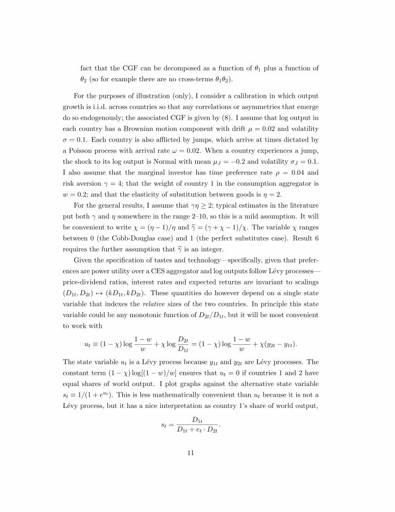
Figure 7: The exorbitant privilege: a visual proof that XS∗B,2 < 0.

in disaster calibrations of the type suggested in Barro (2006), and in the numerical

example used in the illustrations. The proofs of the next two results, and specifically

Figures 7b and 9b, will reveal why the CDP is formulated as it is.

When exchangeability and the CDP hold, the large country’s bond earns a neg-

ative risk premium in foreign units—a type of “exorbitant privilege” (Gourinchas

and Rey (2007), quoting Valery Giscard d’Estaing).

Result 9 (An exorbitant privilege). Suppose Properties 1 and 2 hold. Then UIP

also fails for the large country, whose bonds pay a negative risk premium in small-

country units: XS∗B,2 < 0.

Proof. From equation (21), XS∗B,2 < 0 if and only if c(0,−γ)−c(1−χ, χ−1)−c(χ−1, 1− χ− γ) > 0. By exchangeability, this is equivalent to showing that c(0,−γ) +

c(−γ, 0)−c(χ−1, 1−χ−γ)−c(1−χ−γ, χ−1)−c(1−χ, χ−1)−c(χ−1, 1−χ) > 0.

Panel (a) of Figure 7 represents this inequality graphically. In panel (b), the four

southwest-most points have been compressed towards their mid-point. By convexity,

this makes the sum smaller. But it remains positive by the CDP, and thus the panel

(a) was also positive. [Note: The CDP was formulated as it was precisely so that

sign patterns like the one in panel (b) would be positive.]

Result 8 showed only that the riskless rate is higher in the small country than

in the large country. Result 9 is stronger: it can be rephrased as saying that the

unfavorable riskless rate differential faced by an investor who borrows at the small

28

country’s interest rate and invests at the large country’s interest rate is sufficiently

large that it overcomes the favorable expected exchange rate movement, i.e. Rf,1 −Rf,2 > FX∗2 .

3.1 The failure of uncovered equity parity

To characterize the risk premia on the two countries’ output claims—and to see the

failure of “uncovered equity parity”—I make a final assumption that the countries

have linked fundamentals. In the lognormal case, for example, we want to rule

out the possibility that the correlation between the two countries’ output growth is

negative so that the small country’s output claim is a hedge. The following definition

is the appropriate one for the general, nonlognormal, case.

Property 3 (Linked fundamentals). The two countries have linked fundamentals if

the CGF is supermodular,5 meaning that for all θ1, θ2, φ1, φ2 in ∆,

c(θ1, θ2)+c(φ1, φ2) ≤ c (max {θ1, φ1} ,max {θ2, φ2})+c (min {θ1, φ1} ,min {θ2, φ2}) .

By Topkis’s (1978) Characterization Theorem, Property 3 holds if

∂2c(θ1, θ2)

∂θ1∂θ2≥ 0 (28)

for all θ1 and θ2 in some open set containing ∆. It immediately follows that the

linked fundamentals property holds (with equality) if output growth is independent

across countries. In any given parametric example, it is easy to check whether (28)

holds. In the lognormal case the cumulant-generating function is quadratic in θ1

and θ2, so (28) implies that the linked fundamentals property is equivalent to the

correlation between the two countries’ log output growth being nonnegative. More

generally, the easiest and best way to understand what supermodularity imposes is

through a diagram: see Figure 8c.

Result 10. Suppose Properties 1, 2 and 3 hold. Then XS∗B,1 ≤ XS∗1 , and there is

a critical value η∗ ∈ (1,∞)—where η∗ = 2 in the lognormal case—such that

0 < XS1 < XS∗1 < XS∗2 < XS2 if η > η∗

0 < XS1 < XS∗2 < XS∗1 < XS2 if η < η∗.

5Vives (1990), Milgrom and Roberts (1990), and Athey (2002) present other applications of

supermodularity, notably to games with strategic complementarities.

29

If the countries have strictly linked fundamentals (i.e. if the inequality in the

definition of Property 3 is strict) and η is sufficiently large then we have a total

ordering of risk premia: XS∗B,2 < 0 < XS∗B,1 < XS1 < XS∗1 < XS∗2 < XS2.

Result 10 extends the model’s predictions regarding bond risk premia to risky

assets. The risk premium on the small country’s output claim is greater in foreign

units than in own units, XS∗1 > XS1, while the risk premium on the large country’s

claim is smaller in foreign units than in own units, XS∗2 < XS2. The size of η

indexes the amount of currency risk. If the goods of the two countries are sufficiently

poor substitutes (η < η∗), then currency risk is so great that the risk premium on

the small country’s output claim in foreign units exceeds the risk premium on the

large country’s claim in foreign units, XS∗1 > XS∗2 , even though the small country

contributes a negligible proportion of the marginal investor’s consumption.

4 Conclusion

This paper’s basic prediction, for which Hassan (2012) provides empirical support,

is that small countries should have higher interest rates than large countries, all

else equal. The fundamental asymmetry is that the marginal investor cares more

about the large country than the small country, since it provides a larger share

of consumption. This means that bad (high-marginal-utility) states are those in

which the large country has bad news. When such states occur, the small country’s

output is in greater relative supply, so its exchange rate depreciates. The small

country’s higher interest rate is compensation for this risk. Since, by construction,

the exchange rate follows a random walk, UIP fails in any calibration.

On the methodological side, the paper makes two contributions. It extends

the results of Martin (2013b) to allow for imperfect substitution between goods;

this is a simple and natural way to generate multiple distinct yield curves in an

equilibrium model with perfectly integrated capital markets. It also introduces the

exchangeability, convex difference, and linked fundamentals properties and shows

how to apply them in diagrammatic proofs. The motivation for doing so is that the

quantitative implications of models that feature jumps are sensitively dependent on

assumptions made about the extreme tails of the driving stochastic processes. The

nonparametric approach taken here offers a novel way to understand the economic

mechanism underpinning the model without tying oneself to a particular calibration.

30

5 References

Alvarez, F., A. Atkeson, and P. J. Kehoe (2007), “If Exchange Rates are Random Walks, Then Al-

most Everything We Say About Monetary Policy is Wrong,” American Economic Review, 97:2:339–

345.

Alvarez, F., and U. J. Jermann (2005), “Using Asset Prices to Measure the Persistence of the Marginal

Utility of Wealth,” Econometrica, 73:6:1977–2016.

Athey, S. (2002), “Monotone Comparative Statics under Uncertainty,” Quarterly Journal of Economics,

117:1:187–223.

Backus, D. K., M. Chernov, and I. W. R. Martin (2011), “Disasters Implied by Equity Index Options,”

Journal of Finance, 66:6:1969–2012.

Backus, D. K., S. Foresi, and C. I. Telmer (2001), “Affine Term Structure Models and the Forward Premium

Anomaly,” Journal of Finance, 56:1:279–304.

Backus, D. K., P. J. Kehoe, and F. E. Kydland (1992), “International Real Business Cycles,” Journal of

Political Economy, 100:4:745–775.

Backus, D. K., and G. W. Smith (1993), “Consumption and Real Exchange Rates in Dynamic Economies

with Non-Traded Goods,” Journal of International Economics, 35:297–316.

Bansal, R., and B. N. Lehmann (1997), “Growth-Optimal Portfolio Restrictions on Asset Pricing Models”,

Macroeconomic Dynamics, 1:333–354.

Bansal, R., and I. Shaliastovich (2010), “A Long-Run Risks Explanation of Predictability Puzzles in Bond

and Currency Markets,” working paper.

Barro, R. J. (2006), “Rare Disasters and Asset Markets in the Twentieth Century,” Quarterly Journal of

Economics, 121:3:823–866.

Brandt, M. W., J. H. Cochrane, and P. Santa-Clara (2006), “International Risk Sharing is Better Than

You Think, or Exchange Rates are Too Smooth,” Journal of Monetary Economics, 53:671–698.

Breeden, D. T. (1979), “An Intertemporal Asset Pricing Model with Stochastic Consumption and Invest-

ment Opportunities,” Journal of Financial Economics, 7:265–296.

Brunnermeier, M. K., S. Nagel, and L. Pedersen (2008), “Carry Trades and Currency Crashes,” in Ace-

moglu, D., K. Rogoff, and M. Woodford (eds.), NBER Macroeconomics Annual, 23:1:313–347,

University of Chicago Press.

Calvet, L. E., J. Y. Campbell, and P. Sodini (2007), “Down or Out: Assessing the Welfare Costs of

Household Investment Mistakes,” Journal of Political Economy 115:5:707–747.

Campbell, J. Y. and R. J. Shiller (1988), “The Dividend-Price Ratio and Expectations of Future Dividends

and Discount Factors,” Review of Financial Studies, 1:3:195–228.

Cochrane, J. H. (2008), “Financial Markets and the Real Economy,” chapter 7 of Rajnish Mehra, ed., The

Handbook of the Equity Premium, Elsevier.

Cochrane, J. H., Longstaff, F. A., and P. Santa-Clara (2008), “Two Trees,” Review of Financial Studies,

21:1:347–385.

Colacito, R., and M. M. Croce (2010), “Risks for the Long Run and the Real Exchange Rate,” working

paper.

Cole, H. L., and M. Obstfeld (1991), “Commodity Trade and International Risk Sharing: How Much Do

Financial Markets Matter?” Journal of Monetary Economics, 28:3–24.

31

Dumas, B., C. R. Harvey, and P. Ruiz (2003), “Are Correlations of Stock Returns Justified by Subsequent

Changes in National Outputs?” Journal of International Money and Finance, 22:777–811.

Dybvig, P. H., J. E. Ingersoll, and S. A. Ross (1996), “Long Forward and Zero-Coupon Rates Can Never

Fall,” Journal of Business, 69:1:1–25.

Farhi, E., S. P. Fraiberger, X. Gabaix, R. Ranciere, and A. Verdelhan (2009), “Crash Risk in Currency

Markets,” working paper.

Fama, E. F. (1984), “Forward and Spot Exchange Rates,” Journal of Monetary Economics, 14:3:319–338.

Frankel, J. A. (1980), “Tests of Rational Expectations in the Forward Exchange Market,” Southern Eco-

nomic Journal, 46:4.

Gourinchas, P. O., and H. Rey (2007), “From World Banker to World Venture Capitalist: U.S. External

Adjustment and the Exorbitant Privilege,” in Richard Clarida, ed., G7 Current Account Imbalances:

Sustainability and Adjustment, University of Chicago Press, IL.

Hansen, L. P., and R. J. Hodrick (1980), “Forward Exchange Rates as Optimal Predictors of Future Spot

Rates: An Econometric Analysis,” Journal of Political Economy, 88:5:829–853.

Hansen, L. P. and R. Jagannathan (1991), “Implications of Security Market Data for Models of Dynamic

Economies,” Journal of Political Economy, 99:2:225–262.

Hansen, L. P. and J. A. Scheinkman (2012), “Recursive Utility in a Markov Environment with Stochastic

Growth,” Proceedings of the National Academy of Sciences, forthcoming.

Hassan, T. A. (2012), “Country Size, Currency Unions, and International Asset Returns,” working paper,

Chicago Booth.

Hollifield, B., and A. Yaron (2003), “The Foreign Exchange Risk Premium: Real and Nominal Factors,”

working paper.

Jurek, J. W. (2009), “Crash-Neutral Currency Carry Trades,” working paper, Princeton University.

Lucas, R. E. (1978), “Asset Prices in an Exchange Economy,” Econometrica, 46:6:1429–1445.

Lustig, H., N. Roussanov, and A. Verdelhan (2009), “Common Risk Factors in Currency Markets,” working

paper.

Martin, I. W. R. (2011), “Simple Variance Swaps,” NBER WP 16884.

Martin, I. W. R. (2013a), “Consumption-Based Asset Pricing with Higher Cumulants,” Review of Economic

Studies, 80:2:745–773.

Martin, I. W. R. (2013b), “The Lucas Orchard,” Econometrica, 81:1:55–111.

Merton, R. C. (1973), “An Intertemporal Capital Asset Pricing Model,” Econometrica, 41:5:867–887.

Milgrom, P., and J. Roberts (1990), “Rationalizability, Learning, and Equilibrium in Games with Strategic

Complementarities,” Econometrica, 58:6:1255–1277.

Piazzesi, M., M. Schneider, and S. Tuzel (2007), “Housing, consumption and asset pricing,” Journal of

Financial Economics, 83:531–569.

Siegel, J. J. (1972), “Risk, interest rates, and the forward exchange,” Quarterly Journal of Economics,

86:303–309.

Stathopoulos, A. (2009), “Asset Prices and Risk Sharing in Open Economies,” working paper, University

of Southern California.

Stockman, A. C., and L. L. Tesar (1995), “Tastes and Technology in a Two-Country Model of the Business

Cycle: Explaining International Comovements,” American Economic Review, 85:1:168–185.

Topkis, D. M. (1978), “Minimizing a Submodular Function on a Lattice,” Operations Research, 26:305–321.

32

Verdelhan, A. (2010), “A Habit-Based Explanation of the Exchange Rate Risk Premium,” Journal of

Finance, 65:1:123–145.

Vives, X. (1990), “Nash Equilibrium with Strategic Complementarities,” Journal of Mathematical Eco-

nomics, 19:305–321.

Zapatero, F. (1995), “Equilibrium Asset Prices and Exchange Rates,” Journal of Economic Dynamics and

Control, 19:787–811.

A Appendix

Recall that χ = (η−1)/η and γ = (γ+χ−1)/χ, and let y1t ≡ y1t+[(1−χ)/χ] logw

and y2t ≡ y2t + [(1 − χ)/χ] log(1 − w), so that ut = χ(y2t − y1t). Finally, write

yit ≡ yit − yi0. The consumption aggregator can be expressed as

Ct =[eχy10+χy1t + eχy20+χy2t

] 1χ,

and the price of good 2 in 1-units is

et =

(1− ww

)1−χ(D1t

D2t

)1−χ=

(1− ww

)(1−χ)/χ· e−[(1−χ)/χ]ut .

If η =∞—the perfect substitutes case—then χ = 1 so et is constant. If, on the

other hand, η = 1, then Ct is a Cobb-Douglas aggregator of the two goods so that

Ct ∝ Dw1tD

1−w2t . It is easy to check that each asset’s price-dividend ratio is then

constant. More generally, from (6), good 1’s price-dividend ratio is

P1

D10= E

∫ ∞0

e−ρt(CtC0

)−χγ (D1t

D10

)χdt

= Cχγ0 ·∫ ∞0

e−ρt E

(eχy1t[

eχy10+χy1t + eχy20+χy2t]γ)dt,

and the price of a zero-coupon bond that pays a unit of good 1 at t is

Zt,1 = E e−ρt(CtC0

)−χγ (D1t

D10

)χ−1= Cχγ0 e−ρt · E

(eχ−1χ·χy1t[

eχy10+χy1t + eχy20+χy2t]γ). (29)

Integrating over t, we find the perpetuity price

B1 = Cχγ0 ·∫ ∞0

e−ρt E

(eχ−1χ·χy1t[

eχy10+χy1t + eχy20+χy2t]γ)dt .

33

Correspondingly, the price-dividend ratio of asset 2 is

P2

D20= Cχγ0 ·

∫ ∞0

e−ρt E

(eχy2t[

eχy10+χy1t + eχy20+χy2t]γ)dt ,

and the price, in 2-units, of the t-period zero-coupon good-2 bond is

Zt,2 = Cχγ0 e−ρt · E

(eχ−1χ·χy2t[

eχy10+χy1t + eχy20+χy2t]γ), (30)

so the price-dividend ratio of the good-2 perpetuity is

B2 = Cχγ0 ·∫ ∞0

e−ρt E

(eχ−1χ·χy2t[

eχy10+χy1t + eχy20+χy2t]γ)dt .

The above six equations each feature an expectation of the form

E(α1, α2) ≡ E

(eα1χy1t+α2χy2t[

eχy10+χy1t + eχy20+χy2t]γ), (31)

for appropriate values of α1 and α2.

Proof of Result 2: Expression (31) can be rewritten

E(α1, α2) = e−χγ(y10+y20)/2 · E

(eχ(α1−γ/2)y1t+χ(α2−γ/2)y2t[

eχ(y20+y2t−y10−y1t)/2 + e−χ(y20+y2t−y10−y1t)/2]γ).

Now, for ω ∈ R and γ > 0,

1(eω/2 + e−ω/2

)γ =

∫ ∞−∞

eiωzF (z) dz ,

where i is the complex number√−1 and F (z) ≡ 1

2π · Γ(γ/2− iz)Γ(γ/2 + iz)/Γ(γ)

is defined in terms of the gamma function (Martin (2013b)). It follows that

E(α1, α2) = e−χγ(y10+y20)/2 · E(eχ(α1−γ/2)y1t+χ(α2−γ/2)y2t

∫ ∞−∞

eiχ(y20+y2t−y10−y1t)zF (z) dz

)= e−χγ(y10+y20)/2

∫ ∞−∞

eiuzF (z) · ec(χ(α1−γ/2−iz),χ(α2−γ/2+iz))t dz. (32)

34

The generic expression we want to evaluate is

Vα1,α2(u) = Cχγ0

∫ ∞0

e−ρt Eeα1χy1t+α2χy2t[

eχ(y10+y1t) + eχ(y20+y2t)]γ dt

=

[eχy10 + eχy20

]γeχγ(y10+y20)/2

∫ ∞0

e−ρt · eχγ(y10+y20)/2 · E(α1, α2) dt

=[eu/2 + e−u/2

]γ ∫ ∞t=0

∫ ∞z=−∞

e−{ρ−c[χ(α1−γ/2−iz),χ(α2−γ/2+iz)]}teiuzF (z) dz dt

=[eu/2 + e−u/2

]γ ∫ ∞−∞

eiuzF (z)

ρ− c [χ(α1 − γ/2− iz), χ(α2 − γ/2 + iz)]dz

using (32). The last equality only holds if Re ρ−c [χ(α1 − γ/2− iz), χ(α2 − γ/2 + iz)] >

0 for all z ∈ R. By Lemma 2 of Martin (2013b), this holds if the (superficially

weaker) restriction that ρ − c [χ(α1 − γ/2), χ(α2 − γ/2)] > 0 holds; I impose this

assumption for the relevant values of α1 and α2.

Proof of Result 3: Using (32) in equations (29) and (30), we have

Zt,1 =(eu/2 + e−u/2

)γ·∫ ∞−∞

eiuzF (z)e−{ρ−c[χ(1−1/χ−γ/2−iz),χ(−γ/2+iz)]}t dz

and

Zt,2 =(eu/2 + e−u/2

)γ·∫ ∞−∞

eiuzF (z)e−{ρ−c[χ(−γ/2−iz),χ(1−1/χ−γ/2+iz)]}t dz.

These give the zero-coupon yields immediately; and the riskless rates follow, using

l’Hopital’s rule to take the limit as t→ 0.

Proof of Result 4: To calculate long rates, we use the method of steepest descent.

The long rate in 1-units is

Y∞,1(u) = limT→∞

− 1

Tlog

{∫ ∞−∞

eiuzF (z)e−{ρ−c[χ(1−1/χ−γ/2−iz),χ(−γ/2+iz)]}T dz

},

so we are interested in a stationary point of ρ−c[χ(1−1/χ−γ/2−iz), χ(−γ/2+iz)],

considered as a function of z ∈ C. If z = ix is pure imaginary, this function

is concave when considered as a function of x ∈ R (Martin (2013b)), and has a

maximum at some ix∗, x∗ ∈ R. If |x∗| < γ/2 then the contour of integration can

be continuously deformed to pass through the stationary point without crossing the

pole of F (z) at iγ/2. In this case, by the method of steepest descent, Y∞,1(u) =

ρ−c[χ(1−1/χ− γ/2+x∗), χ(−γ/2−x∗)]. If on the other hand the stationary point

35

occurs for x∗ > γ/2, then we must take the residue at z = iγ/2 into account: in this

case, Y∞,1(u) = ρ− c[χ− 1, 1− χ− γ]. Similarly, if the stationary point occurs at

x∗ < −γ/2 then Y∞,1(u) = ρ− c[−γ, 0]. These cases can be summarized by writing

Y∞,1 = maxθ∈[−γ/2,γ/2] ρ − c[χ(1 − 1/χ − γ/2 + θ), χ(−γ/2 − θ)], or equivalently,

Y∞,1 = maxθ∈[0,γ+χ−1] ρ− c(θ − γ,−θ).The long rate in 2-units follows by interchanging the roles of countries 1 and 2,

which corresponds to switching the arguments of the CGF.

When the exchangeability property holds, it is immediate that long rates are

equal. To get the closed-form solution, use exchangeability to rewrite equation (16)

as Y∞,1 = maxθ∈[0,γ+χ−1] ρ − 12c(θ − γ,−θ) −

12c(−θ, θ − γ). Differentiating, the

maximum is attained at θ = γ/2 (which lies in the admissible region, i.e. γ/2 ≤γ + χ− 1, because γη ≥ 2).

The final statement holds because (17) can be rewritten as

Y∞,2 = maxθ∈[1−χ,γ]

ρ− c(θ − γ,−θ). (33)

Thus if the maximum in (16) is attained for θ in the open set (1 − χ, γ + χ − 1),

then it is attained at the same point in (33).

Expected returns in 1-units Expected returns in 2-units

α1 α2 λ1 λ2 α1 α2 λ1 λ2

tree 1 1 0 1 0 1 0 χ 1− χtree 2 0 1 1− χ χ 0 1 0 1

bond 1 1− 1/χ 0 0 0 1− 1/χ 0 χ− 1 1− χbond 2 0 1− 1/χ 1− χ χ− 1 0 1− 1/χ 0 0

Table 2: Values of α1, α2, λ1, λ2 for Result 6.

Proof of Result 6: The dividend yield is provided by Result 2. Since

P = eλ1y1t+λ2y2t(eχ(y1t−y2t)/2 + eχ(y2t−y1t)/2

)γ ∫ ∞−∞

eiχ(y2t−y1t)zF (z)

ρ− c[χ(α1 − γ/2− iz), χ(α2 − γ/2 + iz)]dz

=

γ∑m=0

(γ

m

)∫ ∞−∞

F (z)ey1t(λ1+mχ−γχ/2−iχz)+y2t(λ2−mχ+γχ/2+iχz)

ρ− c[χ(α1 − γ/2− iz), χ(α2 − γ/2 + iz)]dz ,

where α1, α2, λ1, λ2, which vary from asset to asset, are supplied in Table 2, we find

36

that E dP equals

γ∑m=0

(γ

m

)∫F (z)c(λ1 +mχ− γχ/2− iχz, λ2 −mχ+ γχ/2 + iχz)ey1t(λ1+mχ−γχ/2−iχz)+y2t(λ2−mχ+γχ/2+iχz)

ρ− c[χ(α1 − γ/2− iz), χ(α2 − γ/2 + iz)]dz

by using (13). Dividing by P and rearranging, the result follows, after defining

Gα1,α2,λ1,λ2(u) to equal

γ∑m=0

(γ

m

)e(γ/2−m)u

∫ ∞−∞

eiuzF (z)c(λ1 +mχ− γχ/2− iχz, λ2 −mχ+ γχ/2 + iχz)

ρ− c[χ(α1 − γ/2− iz), χ(α2 − γ/2 + iz)]dz.

Proof of Result 7: Follows the proof of Proposition 6 in Martin (2013b).

Proof of Result 10: Figure 8 establishes that XS1 > 0. Figure 9 shows that

XS1 < XS∗1 ; the proof that XS1 < XS∗2 is almost identical. Figure 10, panel (a)

shows that XS∗1 < XS2; the proof that XS∗2 < XS2 is almost identical. The final

inequality that holds independent of conditions on η is that XS∗B,1 ≤ XS∗1 . This is

established in Figure 10, panel (b).

The remaining inequalities are easier to derive algebraically. By exchangeability,

the sign of XS∗2−XS∗1 is the same as the sign of Q(χ) ≡ c(χ−1, 1−χ−γ)+c(1−χ−γ, χ−1)−c(0, 1−γ)−c(1−γ, 0)−c(0,−γ)−c(−γ, 0)+c(χ, 1−χ−γ)+c(1−χ−γ, χ).

Now, Q(0) = c(−1, 1 − γ) + c(1 − γ,−1) − c(0,−γ) − c(−γ, 0) < 0 and Q(1) =

−c(0, 1 − γ) − c(1 − γ, 0) + c(1,−γ) + c(−γ, 1) > 0 by strict convexity of c(·, ·).Note that Q(χ) is continuous and strictly convex, so Q(χ∗) = 0 for some unique

χ∗ ∈ (0, 1). Defining η∗ via χ∗ = 1 − 1/η∗, we have XS∗2 = XS∗1 if η = η∗;

XS∗2 < XS∗1 for η < η∗; and XS∗2 > XS∗1 for η > η∗.

It remains to be shown that XS∗B,1 < XS1 if the CGF is strictly supermodular

and η is sufficiently large; equivalently, c(χ − 1, 1 − χ) + c(0,−γ) − 2c(χ − 1, 1 −χ − γ) − c(1, 0) + c(χ, 1 − χ − γ) < 0. In the case χ = 1, we must show that

c(0,−γ) + c(1, 0) − c(1,−γ) > 0 = c(0, 0). This follows by strict supermodularity.

Therefore by continuity, XS∗B,1 < XS1 for χ in some neighborhood of 1; equivalently,

XS∗B,1 < XS1 for sufficiently large η.

37

Χ-1 1ΧΘ1

1- Χ-Γ

Θ2

Å

Å �

(a) This is positive because. . .

Χ-1 1ΧΘ1

1- Χ-Γ

Θ2

ÅÅ ��

(b) . . . this is, by convexity. . .

Χ-1 1ΧΘ1

1- Χ-Γ

Θ2

Å

Å

�

�

(c) . . . and this is, by supermodularity

Figure 8: The risk premium on the small country’s output claim is positive in own

units, XS1 > 0. The top panel, which represents XS1, is the sum of the bottom

two panels. Now, panel (b) is strictly positive by convexity of the CGF and panel

(c) is nonnegative by supermodularity. (The CGF is zero at the origin, so the top

panel really is the sum of the bottom two panels.)

Note: panel (c) illustrates what supermodularity “is”, namely the property that

every rectangle whose edges are parallel to the axes and that has this sign pattern

is positive.

38

Χ-1 1- Χ Χ-Γ 11- Χ-ΓΘ1

Χ-1

1- Χ

Χ

-Γ

1

1- Χ-Γ

Θ2

Å

Å

�

�

Å

Å

�

�

(a) To prove this is positive. . .

Χ-1 1- Χ Χ-Γ 11- Χ-ΓΘ1

Χ-1

1- Χ

Χ

-Γ

1

1- Χ-Γ

Θ2

Å

Å

�

�

Å

Å

�

�

(b) . . . use convexity then CDP

Figure 9: The risk premium on the small country’s output claim is higher in foreign

units than it is in own units, XS1 < XS∗1 . The logic is as in Figure 7. (An almost

identical argument shows that XS1 < XS∗2 .)

1- Χ-Γ Χ1-Γ 11- ΧΘ1

1-Γ

1- Χ

Χ

1

1- Χ-Γ

Θ2

Å

Å

�

�

�

�

Å

Å

(a) Positive by convexity

Χ-1 ΧΘ1

1- Χ-Γ

1- Χ

Θ2

Å

Å

�

�

(b) Positive by supermodularity

Figure 10: Left: The risk premium on the large country’s output claim, in large-

country units, is higher than the risk premium on the small country’s output claim,

in large-country units, XS∗1 < XS2. The two groups of points are both positive by

convexity of the CGF. An almost identical argument shows that XS∗2 < XS2.

Right: In large-country units, the small country’s output claim requires a (weakly)

higher risk premium than its bond, XS∗B,1 ≤ XS∗1 . The result follows by supermod-

ularity.

39