Embed Size (px)
Citation preview
Comparison of cell-centered and node-centered
formulations of a high-resolution well-balanced finite
volume scheme: application to shallow water flows
Dr Argiris I. Delis
Dr Ioannis K. Nikolos (TUC)
Maria Kazolea (TUC)
Department of Sciences-Division of Mathematics
Technical University of Crete (TUC), Chania, Greece
CMWR 2010, Barcelona
By the words of Morton and Sonar (Acta Numerica, 2007):
"The jury was out there for a long time in the judgment between cell-center
and vertex-center methods"
CMWR 2010, Barcelona 1
Overview
Ü The 2D nonlinear shallow water model
CMWR 2010, Barcelona 2
Overview
Ü The 2D nonlinear shallow water model
Ü Different grids and grid terminology used in this work
CMWR 2010, Barcelona 2
Overview
Ü The 2D nonlinear shallow water model
Ü Different grids and grid terminology used in this work
Ü Finite volumes on triangles: The node-center (NCFV) and cell-center
(CCFV) approach, in a unified framework
CMWR 2010, Barcelona 2
Overview
Ü The 2D nonlinear shallow water model
Ü Different grids and grid terminology used in this work
Ü Finite volumes on triangles: The node-center (NCFV) and cell-center
(CCFV) approach, in a unified framework
Ü Considerations and improved linear reconstruction for the CCFV
approach
CMWR 2010, Barcelona 2

Overview
Ü The 2D nonlinear shallow water model
Ü Different grids and grid terminology used in this work
Ü Finite volumes on triangles: The node-center (NCFV) and cell-center
(CCFV) approach, in a unified framework
Ü Considerations and improved linear reconstruction for the CCFV
approach
Ü Topography discretisation and wet/dry front treatment.
CMWR 2010, Barcelona 2
Overview
Ü The 2D nonlinear shallow water model
Ü Different grids and grid terminology used in this work
Ü Finite volumes on triangles: The node-center (NCFV) and cell-center
(CCFV) approach, in a unified framework
Ü Considerations and improved linear reconstruction for the CCFV
approach
Ü Topography discretisation and wet/dry front treatment.
Ü Convergence tests, on different grids, for problems with known analytical
solutions
Ü The Malpasset dam case
CMWR 2010, Barcelona 2

Overview
Ü The 2D nonlinear shallow water model
Ü Different grids and grid terminology used in this work
Ü Finite volumes on triangles: The node-center (NCFV) and cell-center
(CCFV) approach, in a unified framework
Ü Considerations and improved linear reconstruction for the CCFV
approach
Ü Topography discretisation and wet/dry front treatment.
Ü Convergence tests, on different grids, for problems with known analytical
solutions
Ü The Malpasset dam case
Ü Conclusions
CMWR 2010, Barcelona 2
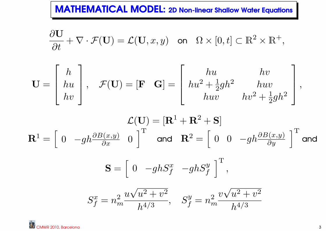
MATHEMATICAL MODEL: 2D Non-linear Shallow Water Equations
∂U
∂t+∇ · F(U) = L(U, x, y) on Ω× [0, t] ⊂ R2 ×R+,
U =
h
hu
hv
, F(U) = [F G] =
hu hv
hu2 + 12gh2 huv
huv hv2 + 12gh2
,
L(U) = [R1 + R2 + S]
R1 =
[0 −gh∂B(x,y)
∂x 0]T
and R2 =
[0 0 −gh∂B(x,y)
∂y
]T
and
S =[
0 −ghSxf −ghSy
f
]T
,
Sxf = n2
m
u√
u2 + v2
h4/3, Sy
f = n2m
v√
u2 + v2
h4/3
CMWR 2010, Barcelona 3

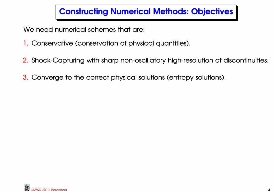
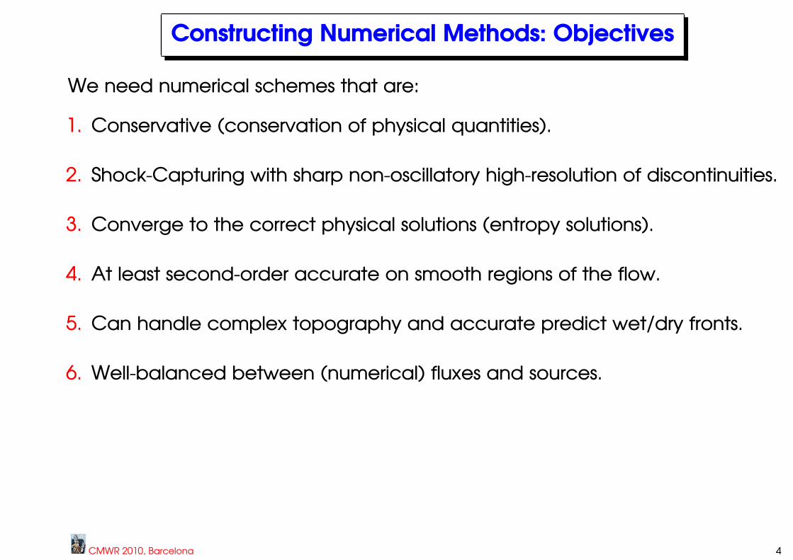
Constructing Numerical Methods: Objectives
We need numerical schemes that are:
1. Conservative (conservation of physical quantities).
CMWR 2010, Barcelona 4

Constructing Numerical Methods: Objectives
We need numerical schemes that are:
1. Conservative (conservation of physical quantities).
2. Shock-Capturing with sharp non-oscillatory high-resolution of discontinuities.
CMWR 2010, Barcelona 4
Constructing Numerical Methods: Objectives
We need numerical schemes that are:
1. Conservative (conservation of physical quantities).
2. Shock-Capturing with sharp non-oscillatory high-resolution of discontinuities.
3. Converge to the correct physical solutions (entropy solutions).
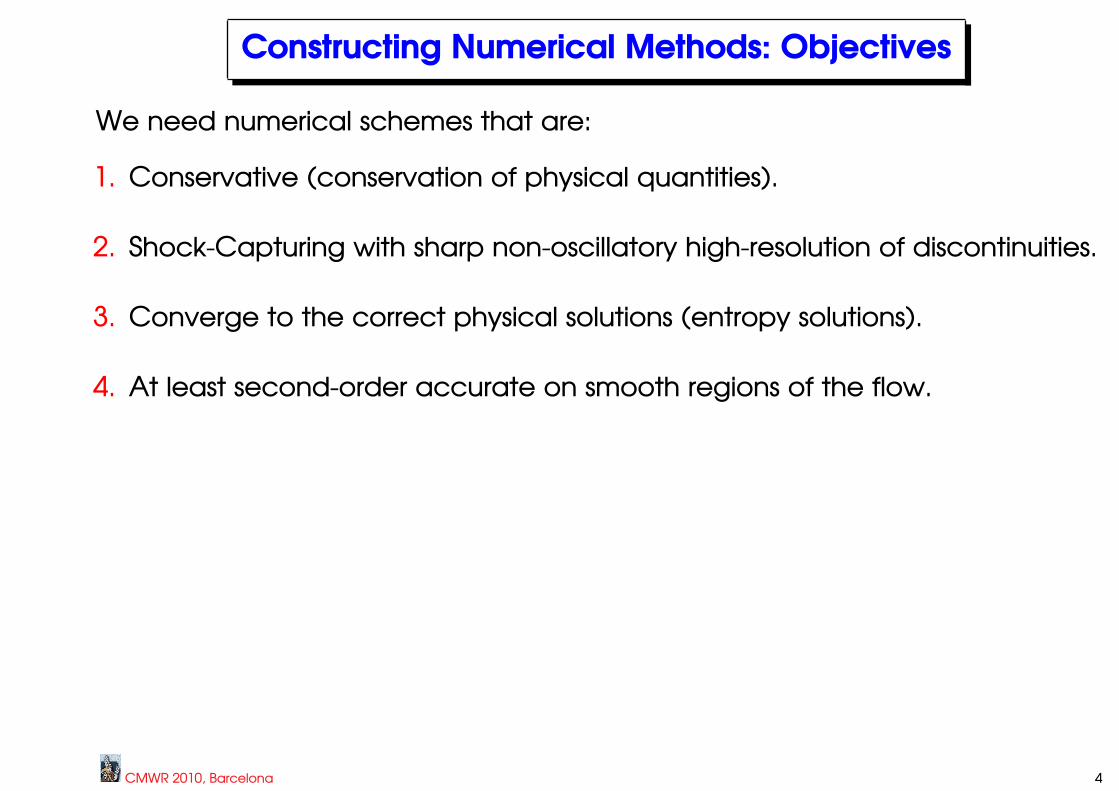
4. At least second-order accurate on smooth regions of the flow.
CMWR 2010, Barcelona 4
Constructing Numerical Methods: Objectives
We need numerical schemes that are:
1. Conservative (conservation of physical quantities).
2. Shock-Capturing with sharp non-oscillatory high-resolution of discontinuities.
3. Converge to the correct physical solutions (entropy solutions).
4. At least second-order accurate on smooth regions of the flow.
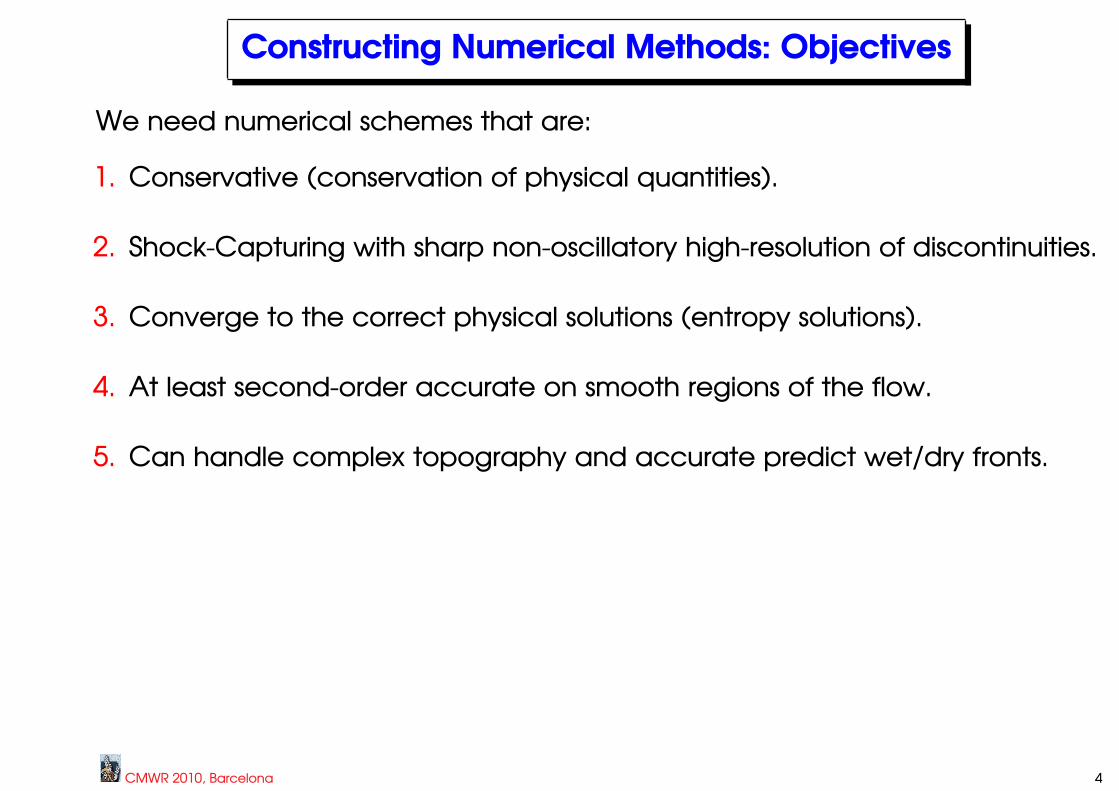
5. Can handle complex topography and accurate predict wet/dry fronts.
CMWR 2010, Barcelona 4
Constructing Numerical Methods: Objectives
We need numerical schemes that are:
1. Conservative (conservation of physical quantities).
2. Shock-Capturing with sharp non-oscillatory high-resolution of discontinuities.
3. Converge to the correct physical solutions (entropy solutions).
4. At least second-order accurate on smooth regions of the flow.
5. Can handle complex topography and accurate predict wet/dry fronts.
6. Well-balanced between (numerical) fluxes and sources.
7. Enable various practical inflow/outflow boundary conditions
CMWR 2010, Barcelona 4
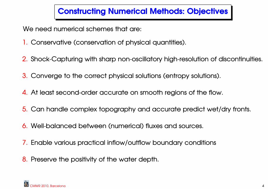
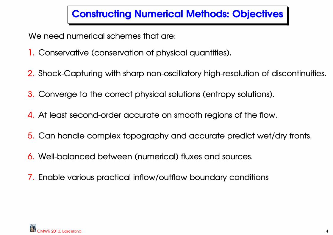
Constructing Numerical Methods: Objectives
We need numerical schemes that are:
1. Conservative (conservation of physical quantities).
2. Shock-Capturing with sharp non-oscillatory high-resolution of discontinuities.
3. Converge to the correct physical solutions (entropy solutions).
4. At least second-order accurate on smooth regions of the flow.
5. Can handle complex topography and accurate predict wet/dry fronts.
6. Well-balanced between (numerical) fluxes and sources.
7. Enable various practical inflow/outflow boundary conditions
8. Preserve the positivity of the water depth.
CMWR 2010, Barcelona 4
Grid Terminilogy
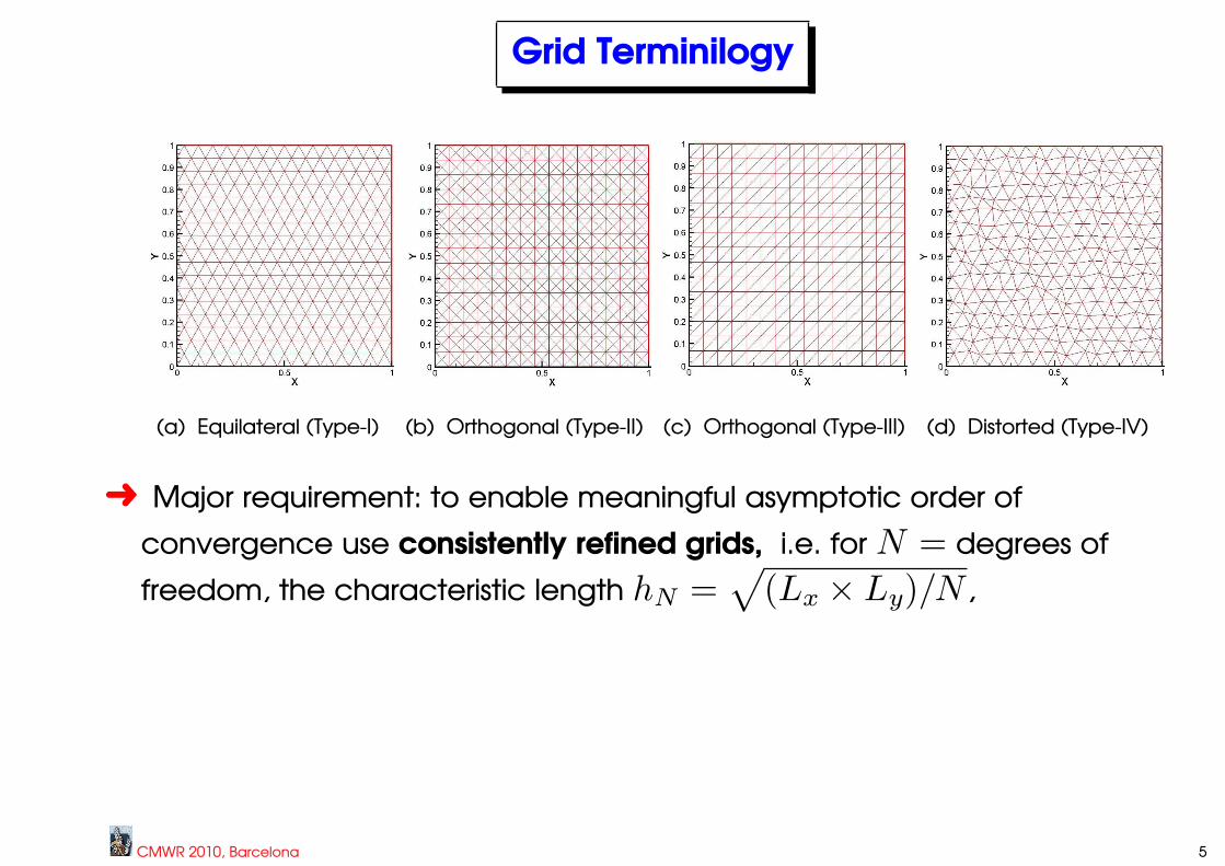
(a) Equilateral (Type-I) (b) Orthogonal (Type-II) (c) Orthogonal (Type-III) (d) Distorted (Type-IV)
CMWR 2010, Barcelona 5
Grid Terminilogy
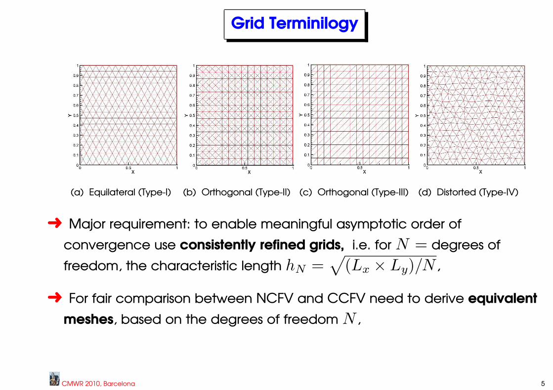
(a) Equilateral (Type-I) (b) Orthogonal (Type-II) (c) Orthogonal (Type-III) (d) Distorted (Type-IV)
Ü Major requirement: to enable meaningful asymptotic order of
convergence use consistently refined grids, i.e. for N = degrees of
freedom, the characteristic length hN =√
(Lx × Ly)/N ,
CMWR 2010, Barcelona 5
Grid Terminilogy
(a) Equilateral (Type-I) (b) Orthogonal (Type-II) (c) Orthogonal (Type-III) (d) Distorted (Type-IV)
Ü Major requirement: to enable meaningful asymptotic order of
convergence use consistently refined grids, i.e. for N = degrees of
freedom, the characteristic length hN =√
(Lx × Ly)/N ,
Ü For fair comparison between NCFV and CCFV need to derive equivalent
meshes, based on the degrees of freedom N ,
CMWR 2010, Barcelona 5
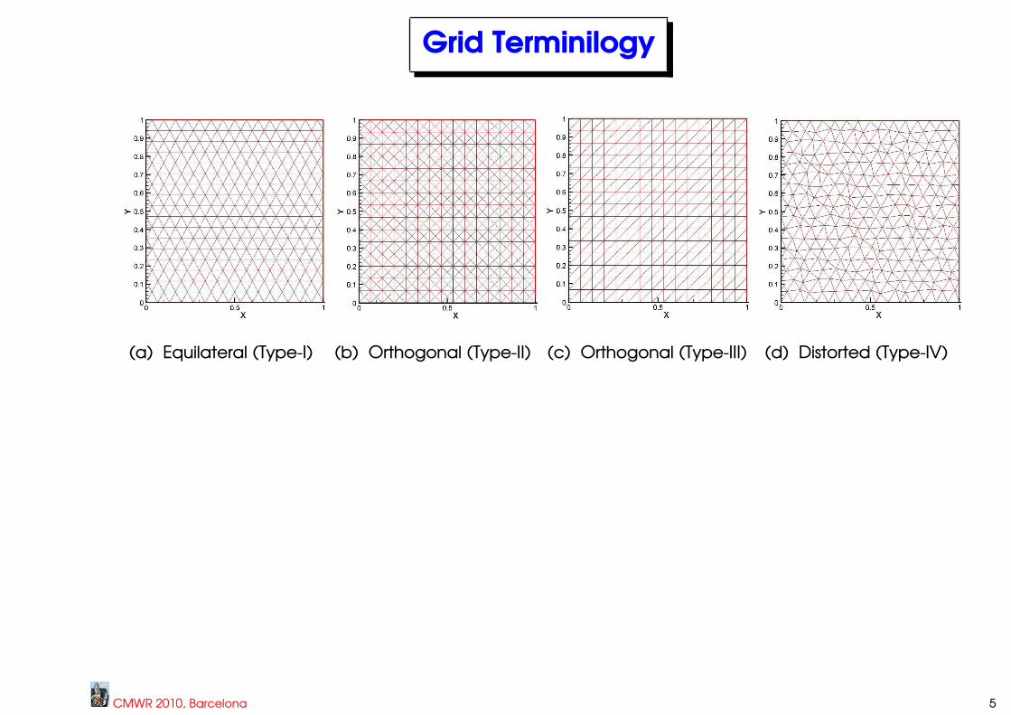
Grid Terminilogy
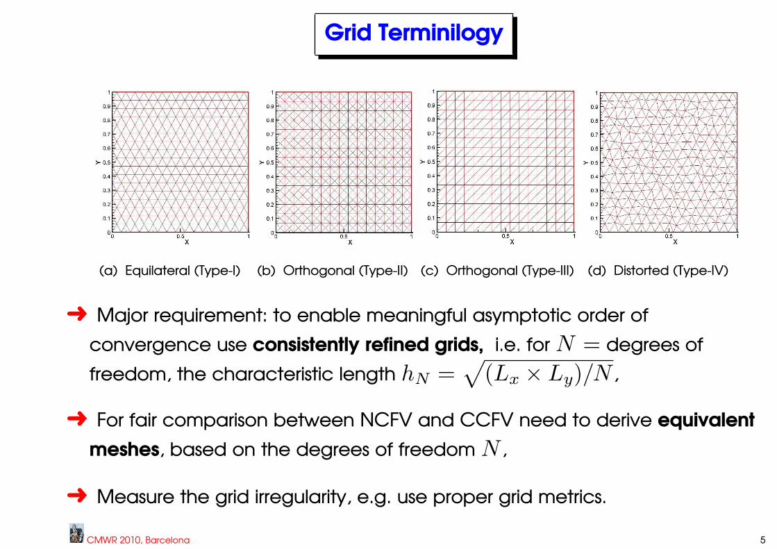
(a) Equilateral (Type-I) (b) Orthogonal (Type-II) (c) Orthogonal (Type-III) (d) Distorted (Type-IV)
Ü Major requirement: to enable meaningful asymptotic order of
convergence use consistently refined grids, i.e. for N = degrees of
freedom, the characteristic length hN =√
(Lx × Ly)/N ,
Ü For fair comparison between NCFV and CCFV need to derive equivalent
meshes, based on the degrees of freedom N ,
Ü Measure the grid irregularity, e.g. use proper grid metrics.
CMWR 2010, Barcelona 5
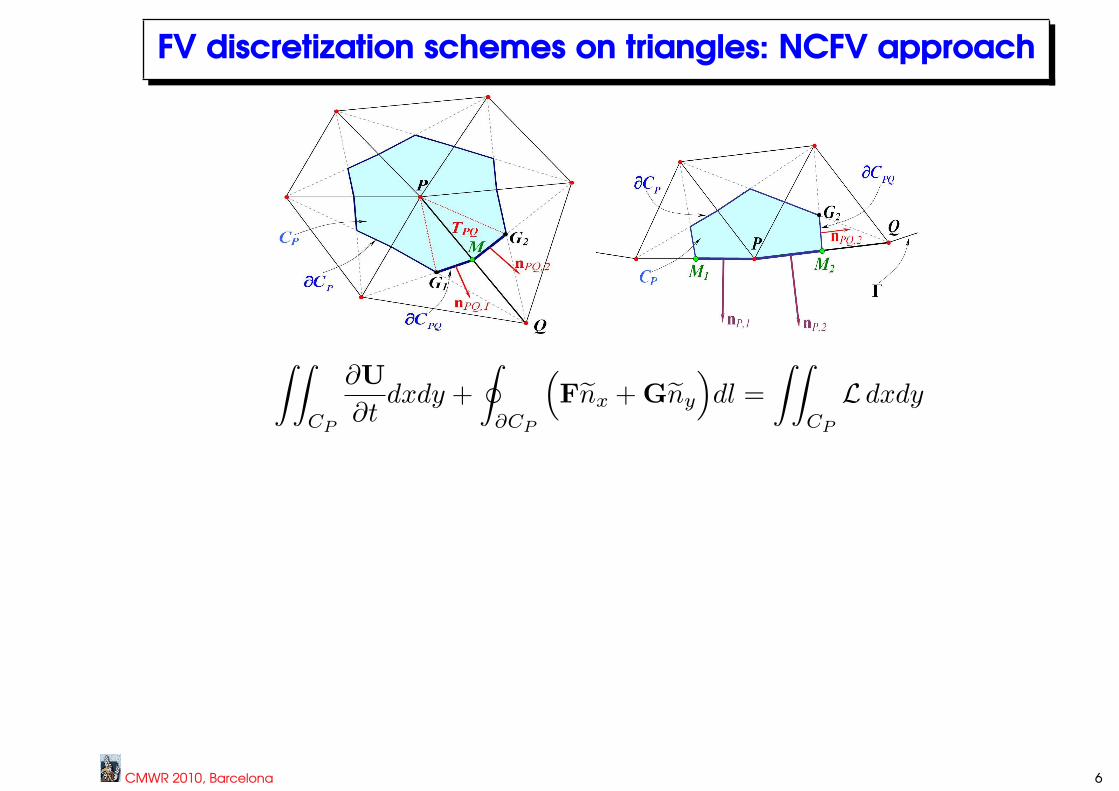
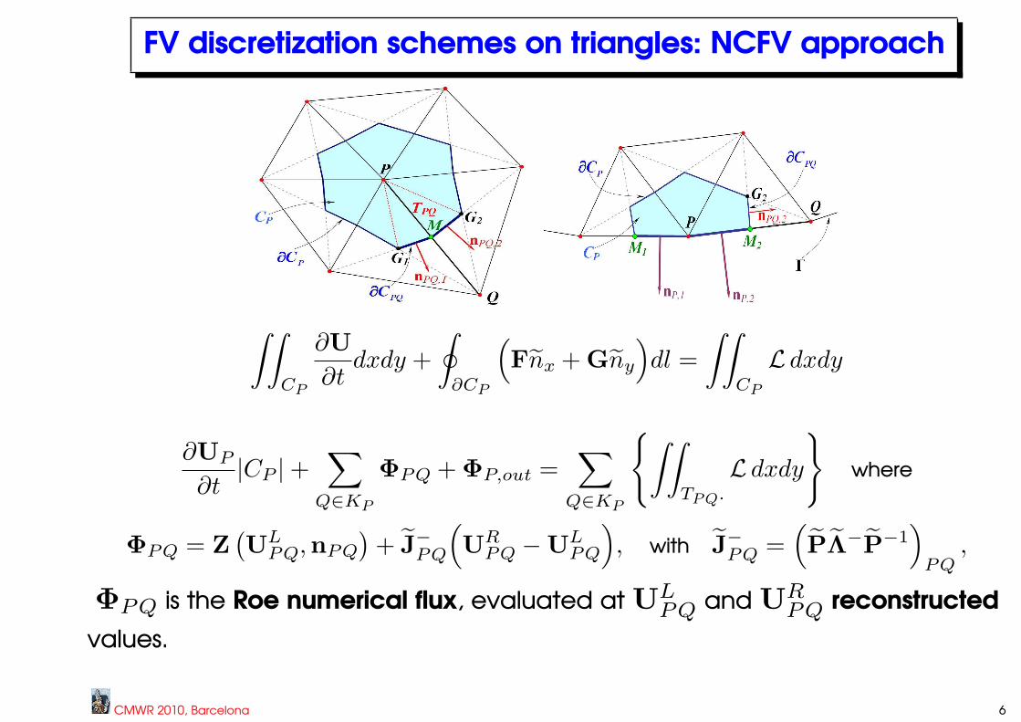
FV discretization schemes on triangles: NCFV approach
∫∫
CP
∂U
∂tdxdy +
∮
∂CP
(Fnx + Gny
)dl =
∫∫
CP
L dxdy
CMWR 2010, Barcelona 6
FV discretization schemes on triangles: NCFV approach
∫∫
CP
∂U
∂tdxdy +
∮
∂CP
(Fnx + Gny
)dl =
∫∫
CP
L dxdy
∂UP
∂t|CP |+
∑
Q∈KP
ΦPQ + ΦP,out =∑
Q∈KP
∫∫
TPQ.
L dxdy
where
ΦPQ = Z(U
LPQ,nPQ
)+ J
−PQ
(U
RPQ −U
LPQ
), with J
−PQ =
(PΛ
−P−1
)
PQ,
ΦPQ is the Roe numerical flux, evaluated at ULPQ and U
RPQ reconstructed
values.
CMWR 2010, Barcelona 6
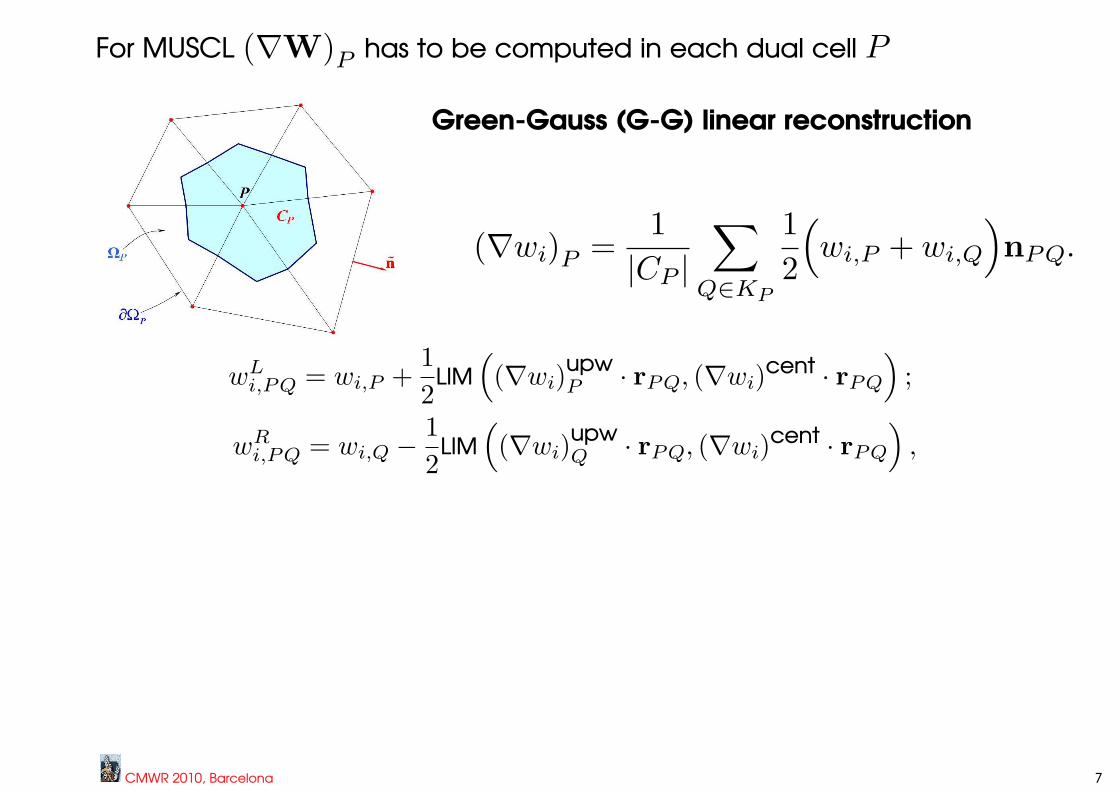
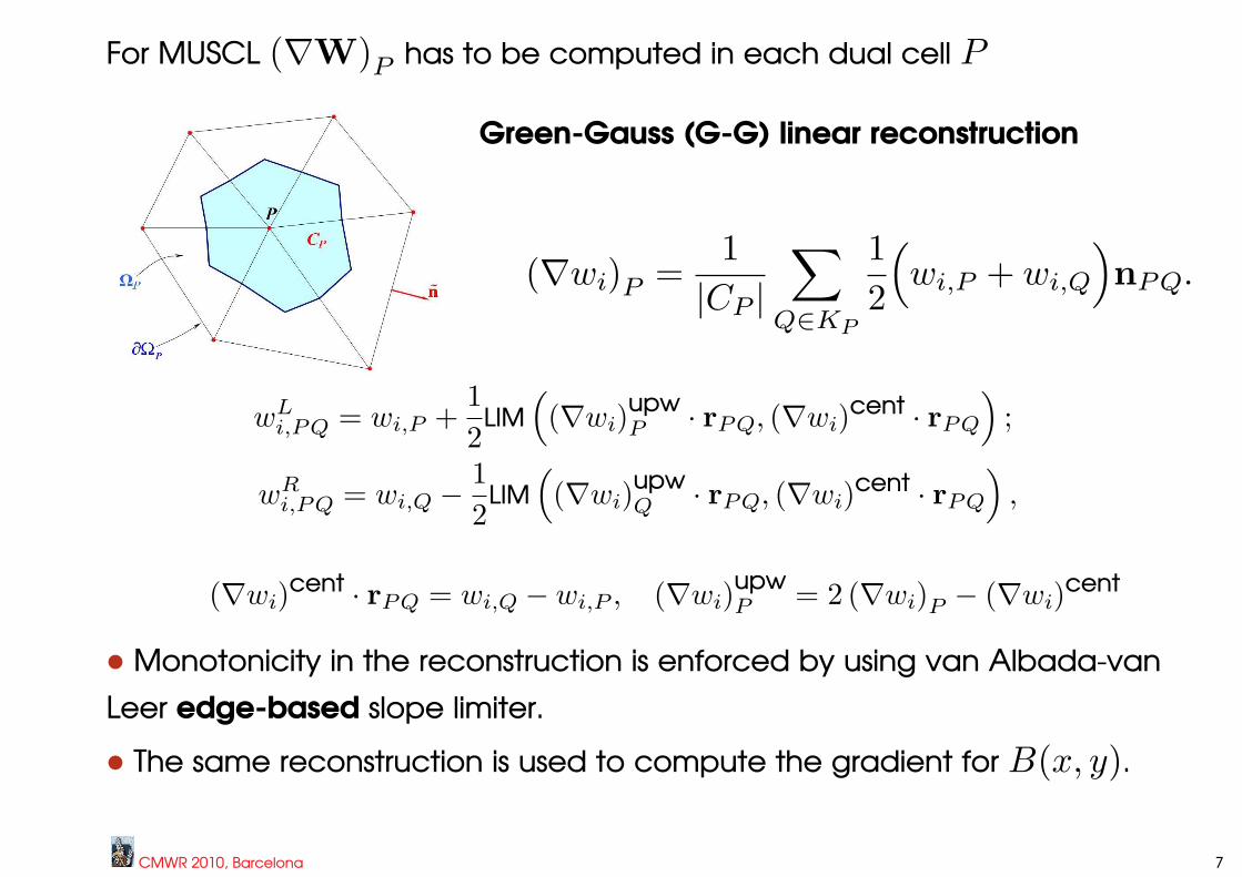
For MUSCL (∇W)P has to be computed in each dual cell P
Green-Gauss (G-G) linear reconstruction
(∇wi)P =1
|CP |∑
Q∈KP
1
2
(wi,P + wi,Q
)nPQ.
wLi,PQ = wi,P +
1
2LIM
((∇wi)
upwP · rPQ, (∇wi)
cent · rPQ
);
wRi,PQ = wi,Q −
1
2LIM
((∇wi)
upwQ · rPQ, (∇wi)
cent · rPQ
),
CMWR 2010, Barcelona 7
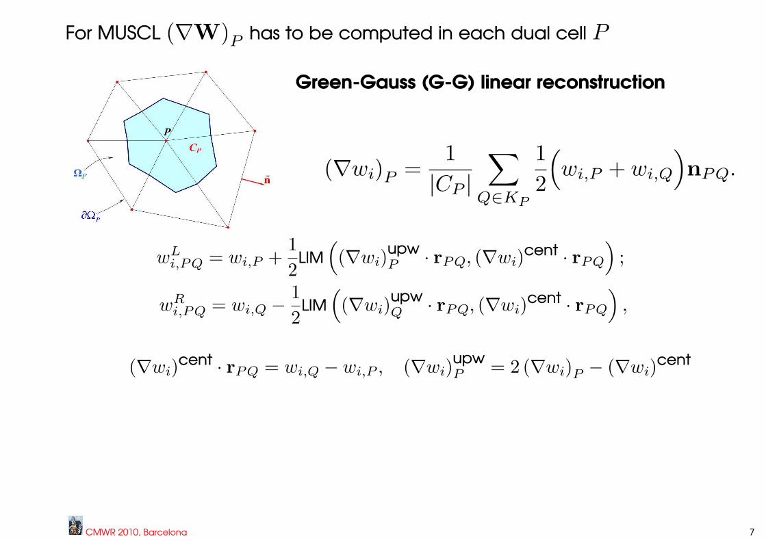
For MUSCL (∇W)P has to be computed in each dual cell P
Green-Gauss (G-G) linear reconstruction
(∇wi)P =1
|CP |∑
Q∈KP
1
2
(wi,P + wi,Q
)nPQ.
wLi,PQ = wi,P +
1
2LIM
((∇wi)
upwP · rPQ, (∇wi)
cent · rPQ
);
wRi,PQ = wi,Q −
1
2LIM
((∇wi)
upwQ · rPQ, (∇wi)
cent · rPQ
),
(∇wi)cent · rPQ = wi,Q − wi,P , (∇wi)
upwP = 2 (∇wi)P − (∇wi)
cent
CMWR 2010, Barcelona 7
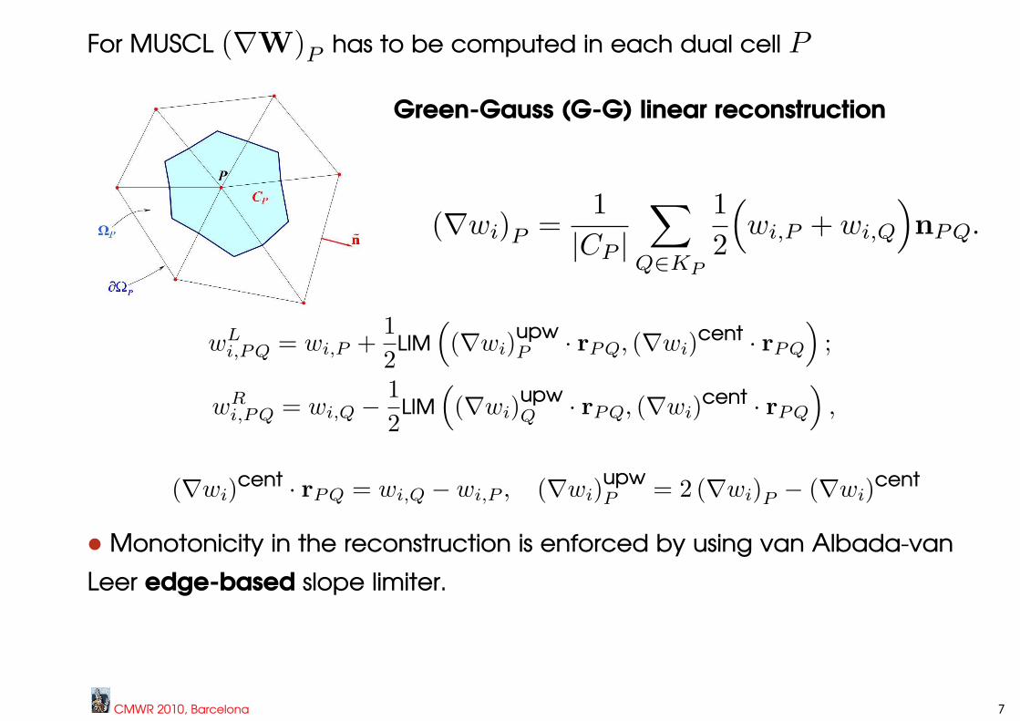
For MUSCL (∇W)P has to be computed in each dual cell P
Green-Gauss (G-G) linear reconstruction
(∇wi)P =1
|CP |∑
Q∈KP
1
2
(wi,P + wi,Q
)nPQ.
wLi,PQ = wi,P +
1
2LIM
((∇wi)
upwP · rPQ, (∇wi)
cent · rPQ
);
wRi,PQ = wi,Q −
1
2LIM
((∇wi)
upwQ · rPQ, (∇wi)
cent · rPQ
),
(∇wi)cent · rPQ = wi,Q − wi,P , (∇wi)
upwP = 2 (∇wi)P − (∇wi)
cent
• Monotonicity in the reconstruction is enforced by using van Albada-van
Leer edge-based slope limiter.
CMWR 2010, Barcelona 7
For MUSCL (∇W)P has to be computed in each dual cell P
Green-Gauss (G-G) linear reconstruction
(∇wi)P =1
|CP |∑
Q∈KP
1
2
(wi,P + wi,Q
)nPQ.
wLi,PQ = wi,P +
1
2LIM
((∇wi)
upwP · rPQ, (∇wi)
cent · rPQ
);
wRi,PQ = wi,Q −
1
2LIM
((∇wi)
upwQ · rPQ, (∇wi)
cent · rPQ
),
(∇wi)cent · rPQ = wi,Q − wi,P , (∇wi)
upwP = 2 (∇wi)P − (∇wi)
cent
• Monotonicity in the reconstruction is enforced by using van Albada-van
Leer edge-based slope limiter.
• The same reconstruction is used to compute the gradient for B(x, y).
CMWR 2010, Barcelona 7
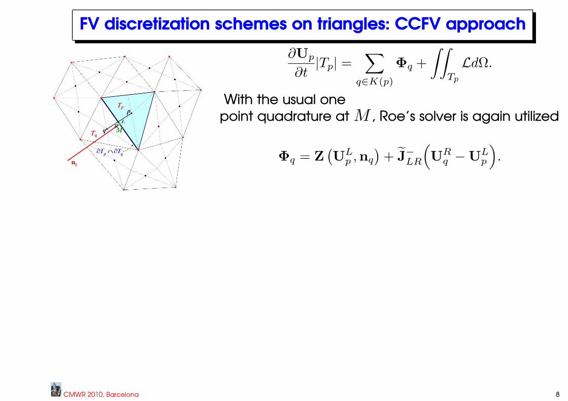
FV discretization schemes on triangles: CCFV approach
∂Up
∂t|Tp| =
∑
q∈K(p)
Φq +
∫∫
Tp
LdΩ.
With the usual one
point quadrature at M , Roe’s solver is again utilized
Φq = Z(U
Lp ,nq
)+ J
−LR
(U
Rq −U
Lp
).
CMWR 2010, Barcelona 8
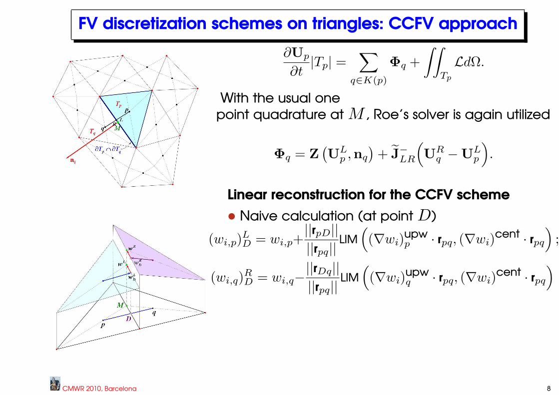
FV discretization schemes on triangles: CCFV approach
∂Up
∂t|Tp| =
∑
q∈K(p)
Φq +
∫∫
Tp
LdΩ.
With the usual one
point quadrature at M , Roe’s solver is again utilized
Φq = Z(U
Lp ,nq
)+ J
−LR
(U
Rq −U
Lp
).
Linear reconstruction for the CCFV scheme
• Naive calculation (at point D)
(wi,p)LD = wi,p+
||rpD||||rpq||
LIM
((∇wi)
upwp · rpq, (∇wi)
cent · rpq
);
(wi,q)RD = wi,q−
||rDq||||rpq||
LIM
((∇wi)
upwq · rpq, (∇wi)
cent · rpq
)
CMWR 2010, Barcelona 8
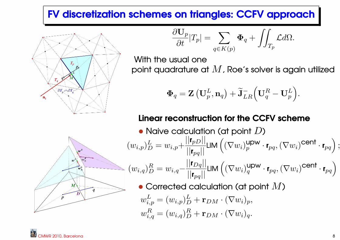
FV discretization schemes on triangles: CCFV approach
∂Up
∂t|Tp| =
∑
q∈K(p)
Φq +
∫∫
Tp
LdΩ.
With the usual one
point quadrature at M , Roe’s solver is again utilized
Φq = Z(U
Lp ,nq
)+ J
−LR
(U
Rq −U
Lp
).
Linear reconstruction for the CCFV scheme
• Naive calculation (at point D)
(wi,p)LD = wi,p+
||rpD||||rpq||
LIM
((∇wi)
upwp · rpq, (∇wi)
cent · rpq
);
(wi,q)RD = wi,q−
||rDq||||rpq||
LIM
((∇wi)
upwq · rpq, (∇wi)
cent · rpq
)
• Corrected calculation (at point M )
wLi,p = (wi,p)
LD + rDM · (∇wi)p,
wRi,q = (wi,q)
RD + rDM · (∇wi)q.
CMWR 2010, Barcelona 8
CCFV approach: Gradient operators
Three element (compact stencil) gradient
∇wi,p =1
|Ccp|
∑
q,r∈K(p)r 6=q
1
2
(wi,q + wi,r
)nqr.
CMWR 2010, Barcelona 9
CCFV approach: Gradient operators
Three element (compact stencil) gradient
∇wi,p =1
|Ccp|
∑
q,r∈K(p)r 6=q
1
2
(wi,q + wi,r
)nqr.
CMWR 2010, Barcelona 9

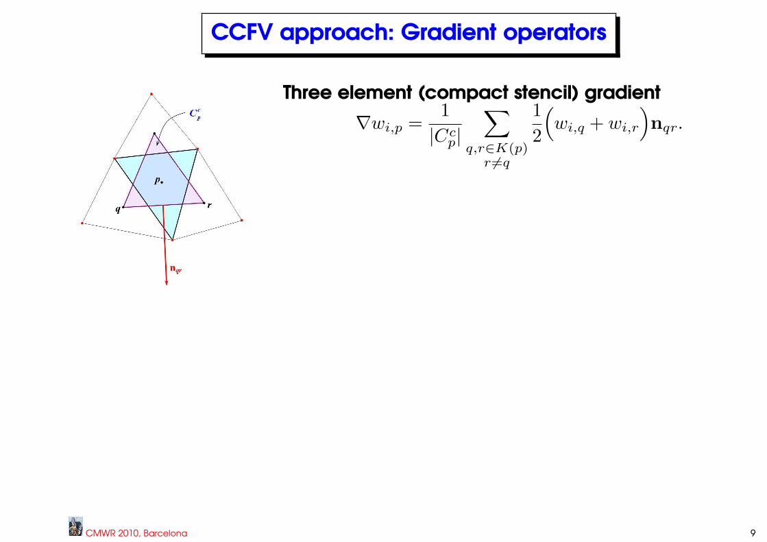
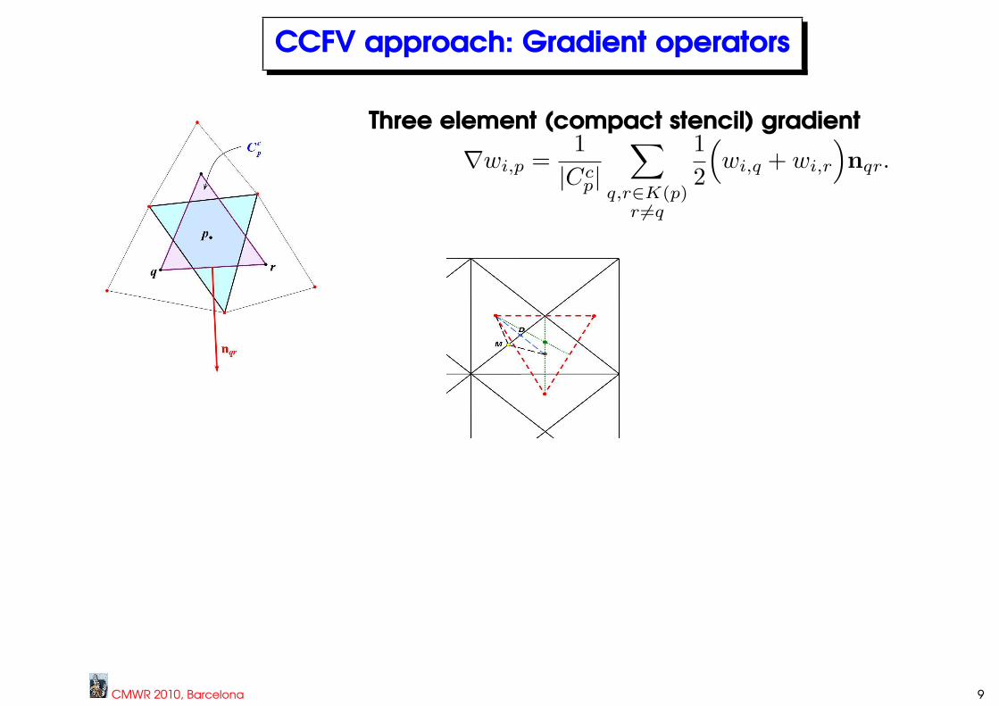
CCFV approach: Gradient operators
Three element (compact stencil) gradient
∇wi,p =1
|Ccp|
∑
q,r∈K(p)r 6=q
1
2
(wi,q + wi,r
)nqr.
Extended element (wide stencil) gradient
∇wi,p =1
|Cwp |
∑
l,r∈K′(p)r 6=l
1
2
(wi,l + wi,r
)nlr
CMWR 2010, Barcelona 9
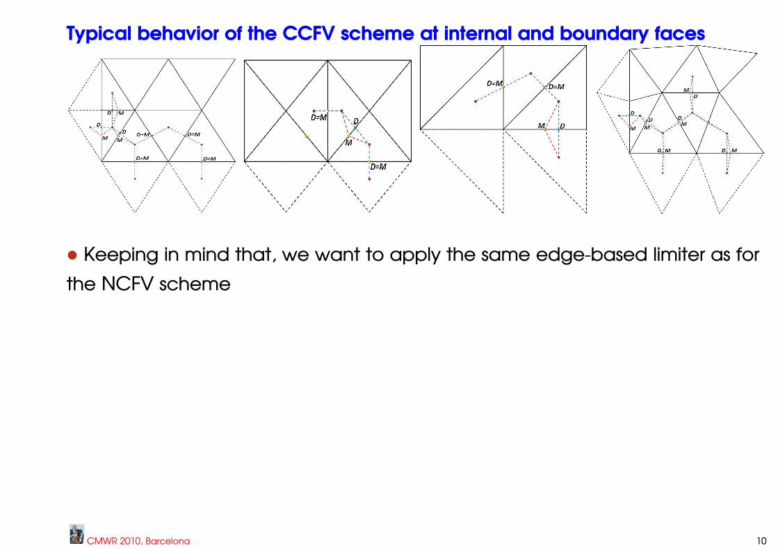
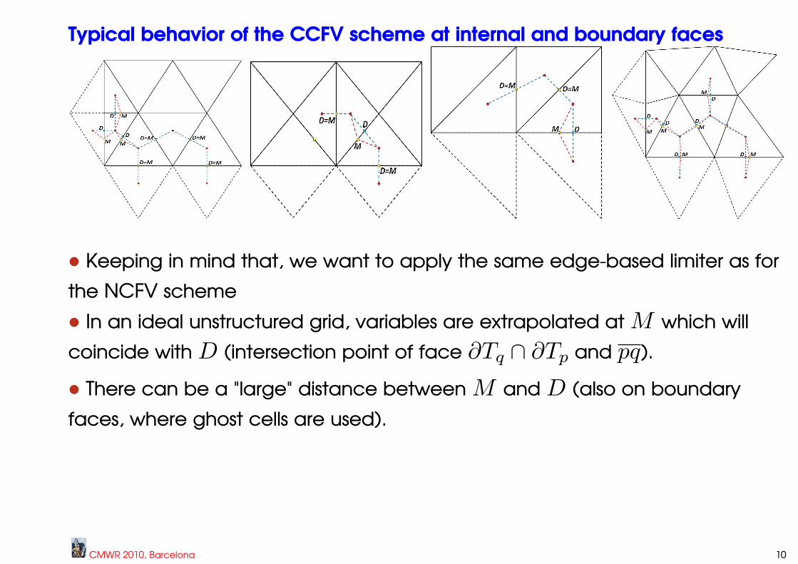
Typical behavior of the CCFV scheme at internal and boundary faces
• Keeping in mind that, we want to apply the same edge-based limiter as for
the NCFV scheme
CMWR 2010, Barcelona 10
Typical behavior of the CCFV scheme at internal and boundary faces
• Keeping in mind that, we want to apply the same edge-based limiter as for
the NCFV scheme
• In an ideal unstructured grid, variables are extrapolated at M which will
coincide with D (intersection point of face ∂Tq ∩ ∂Tp and pq).
CMWR 2010, Barcelona 10
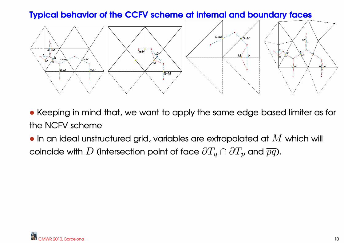
Typical behavior of the CCFV scheme at internal and boundary faces
• Keeping in mind that, we want to apply the same edge-based limiter as for
the NCFV scheme
• In an ideal unstructured grid, variables are extrapolated at M which will
coincide with D (intersection point of face ∂Tq ∩ ∂Tp and pq).
• There can be a "large" distance between M and D (also on boundary
faces, where ghost cells are used).
CMWR 2010, Barcelona 10
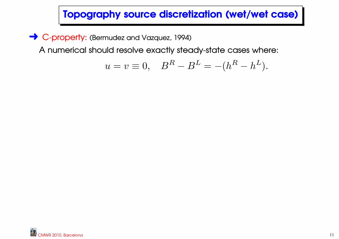
Topography source discretization (wet/wet case)
Ü C-property: (Bermudez and Vazquez, 1994)
A numerical should resolve exactly steady-state cases where:
u = v ≡ 0, BR −BL = −(hR − hL).
CMWR 2010, Barcelona 11
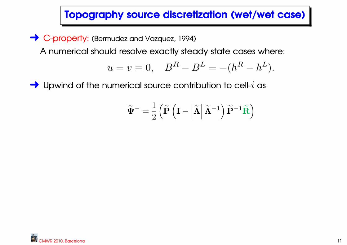
Topography source discretization (wet/wet case)
Ü C-property: (Bermudez and Vazquez, 1994)
A numerical should resolve exactly steady-state cases where:
u = v ≡ 0, BR −BL = −(hR − hL).
Ü Upwind of the numerical source contribution to cell-i as
Ψ− =
1
2
(P
(I−
∣∣∣Λ∣∣∣ Λ−1
)P−1
R
)
CMWR 2010, Barcelona 11
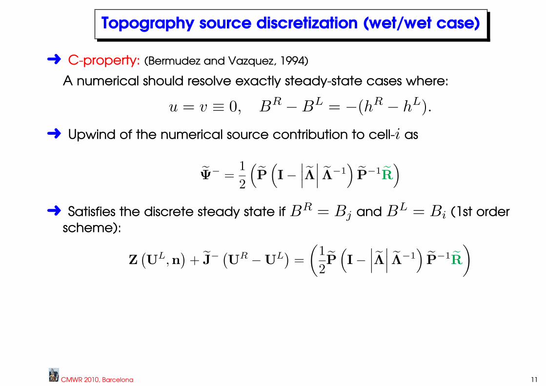
Topography source discretization (wet/wet case)
Ü C-property: (Bermudez and Vazquez, 1994)
A numerical should resolve exactly steady-state cases where:
u = v ≡ 0, BR −BL = −(hR − hL).
Ü Upwind of the numerical source contribution to cell-i as
Ψ− =
1
2
(P
(I−
∣∣∣Λ∣∣∣ Λ−1
)P−1
R
)
Ü Satisfies the discrete steady state if BR = Bj and BL = Bi (1st order
scheme):
Z(U
L,n)
+ J−(U
R −UL)
=
(1
2P
(I−
∣∣∣Λ∣∣∣ Λ−1
)P−1
R
)
when
R =
0
−ghL + hR
2
(BR −BL
)nx
−ghL + hR
2
(BR −BL
)ny
CMWR 2010, Barcelona 11
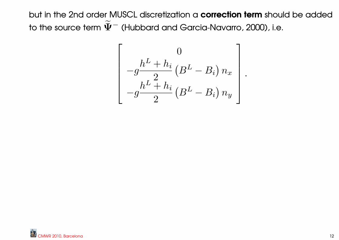
but in the 2nd order MUSCL discretization a correction term should be added
to the source term Ψ− (Hubbard and Garcia-Navarro, 2000), i.e.
0
−ghL + hi
2
(BL −Bi
)nx
−ghL + hi
2
(BL −Bi
)ny
.
CMWR 2010, Barcelona 12
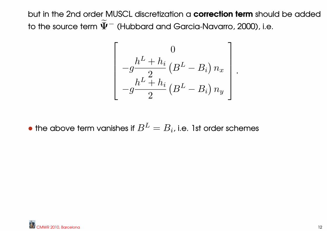
but in the 2nd order MUSCL discretization a correction term should be added
to the source term Ψ− (Hubbard and Garcia-Navarro, 2000), i.e.
0
−ghL + hi
2
(BL −Bi
)nx
−ghL + hi
2
(BL −Bi
)ny
.
• the above term vanishes if BL = Bi, i.e. 1st order schemes
CMWR 2010, Barcelona 12
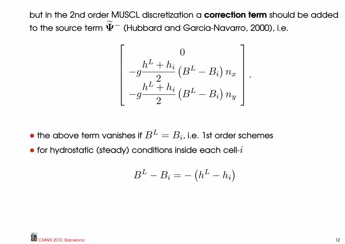
but in the 2nd order MUSCL discretization a correction term should be added
to the source term Ψ− (Hubbard and Garcia-Navarro, 2000), i.e.
0
−ghL + hi
2
(BL −Bi
)nx
−ghL + hi
2
(BL −Bi
)ny
.
• the above term vanishes if BL = Bi, i.e. 1st order schemes
• for hydrostatic (steady) conditions inside each cell-i
BL −Bi = −(hL − hi
)
CMWR 2010, Barcelona 12
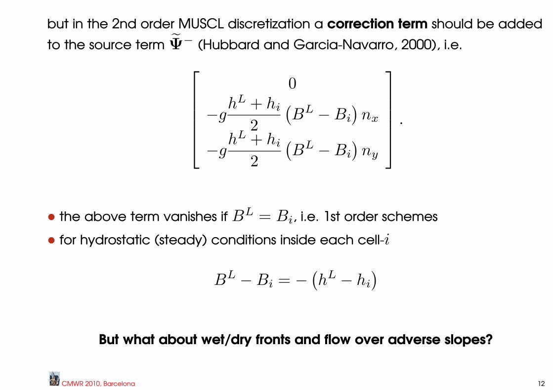
but in the 2nd order MUSCL discretization a correction term should be added
to the source term Ψ− (Hubbard and Garcia-Navarro, 2000), i.e.
0
−ghL + hi
2
(BL −Bi
)nx
−ghL + hi
2
(BL −Bi
)ny
.
• the above term vanishes if BL = Bi, i.e. 1st order schemes
• for hydrostatic (steady) conditions inside each cell-i
BL −Bi = −(hL − hi
)
But what about wet/dry fronts and flow over adverse slopes?
CMWR 2010, Barcelona 12
Topography source discretization (wet/dry case)
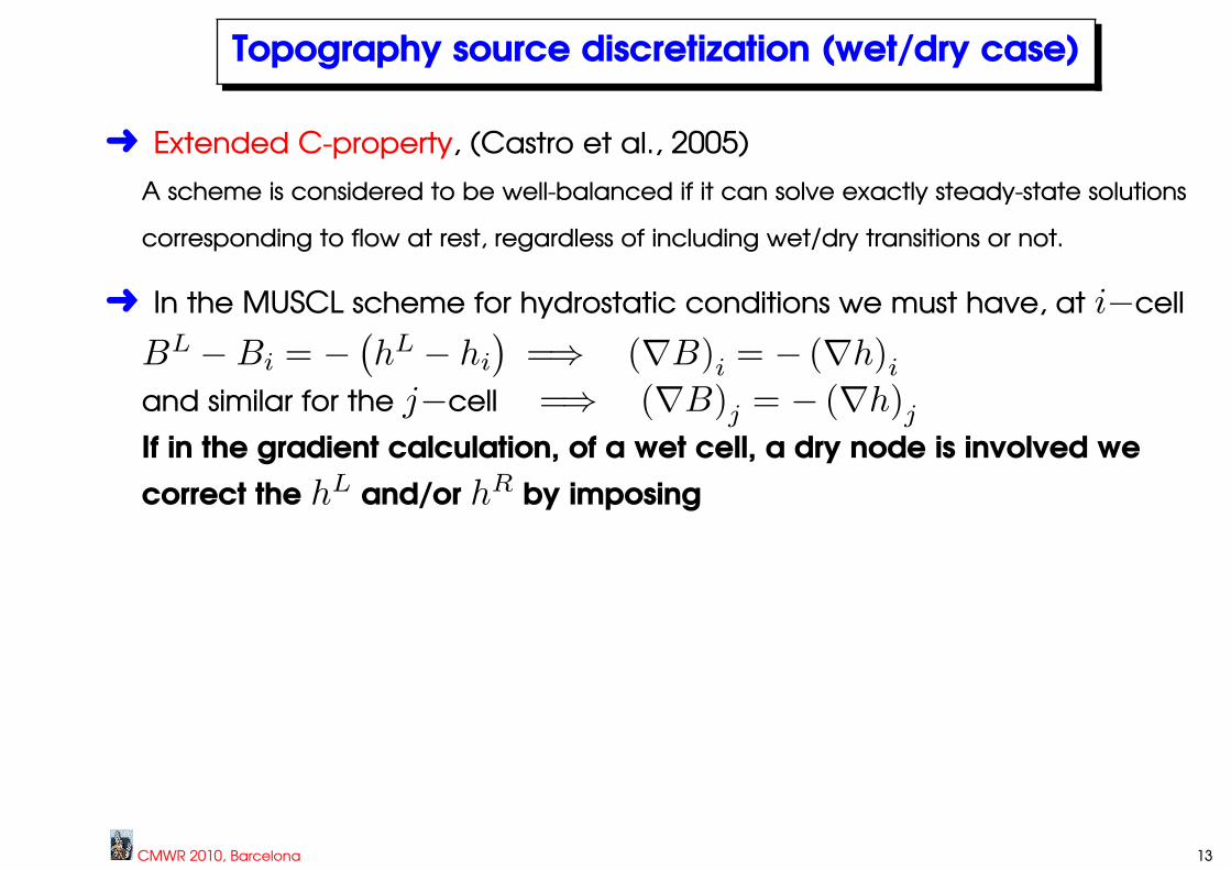
Ü Extended C-property, (Castro et al., 2005)
A scheme is considered to be well-balanced if it can solve exactly steady-state solutions
corresponding to flow at rest, regardless of including wet/dry transitions or not.
Ü In the MUSCL scheme for hydrostatic conditions we must have, at i−cell
CMWR 2010, Barcelona 13
Topography source discretization (wet/dry case)
Ü Extended C-property, (Castro et al., 2005)
A scheme is considered to be well-balanced if it can solve exactly steady-state solutions
corresponding to flow at rest, regardless of including wet/dry transitions or not.
Ü In the MUSCL scheme for hydrostatic conditions we must have, at i−cell
BL −Bi = −(hL − hi
)
CMWR 2010, Barcelona 13
Topography source discretization (wet/dry case)
Ü Extended C-property, (Castro et al., 2005)
A scheme is considered to be well-balanced if it can solve exactly steady-state solutions
corresponding to flow at rest, regardless of including wet/dry transitions or not.
Ü In the MUSCL scheme for hydrostatic conditions we must have, at i−cell
BL −Bi = −(hL − hi
)=⇒ (∇B)i = − (∇h)i
and similar for the j−cell =⇒ (∇B)j = − (∇h)j
If in the gradient calculation, of a wet cell, a dry node is involved we
correct the hL and/or hR by imposing
CMWR 2010, Barcelona 13

Topography source discretization (wet/dry case)
Ü Extended C-property, (Castro et al., 2005)
A scheme is considered to be well-balanced if it can solve exactly steady-state solutions
corresponding to flow at rest, regardless of including wet/dry transitions or not.
Ü In the MUSCL scheme for hydrostatic conditions we must have, at i−cell
BL −Bi = −(hL − hi
)=⇒ (∇B)i = − (∇h)i
and similar for the j−cell =⇒ (∇B)j = − (∇h)j
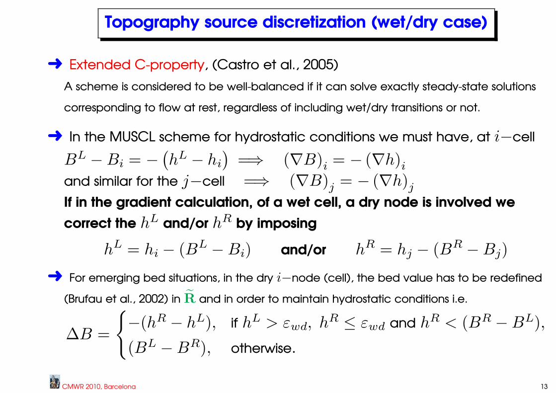
If in the gradient calculation, of a wet cell, a dry node is involved we
correct the hL and/or hR by imposing
hL = hi − (BL −Bi) and/or hR = hj − (BR −Bj)
CMWR 2010, Barcelona 13
Topography source discretization (wet/dry case)
Ü Extended C-property, (Castro et al., 2005)
A scheme is considered to be well-balanced if it can solve exactly steady-state solutions
corresponding to flow at rest, regardless of including wet/dry transitions or not.
Ü In the MUSCL scheme for hydrostatic conditions we must have, at i−cell
BL −Bi = −(hL − hi
)=⇒ (∇B)i = − (∇h)i
and similar for the j−cell =⇒ (∇B)j = − (∇h)j
If in the gradient calculation, of a wet cell, a dry node is involved we
correct the hL and/or hR by imposing
hL = hi − (BL −Bi) and/or hR = hj − (BR −Bj)
Ü For emerging bed situations, in the dry i−node (cell), the bed value has to be redefined
(Brufau et al., 2002) in R and in order to maintain hydrostatic conditions i.e.
∆B =
−(hR − hL), if hL > εwd, hR ≤ εwd and hR < (BR −BL),
(BL −BR), otherwise.
CMWR 2010, Barcelona 13
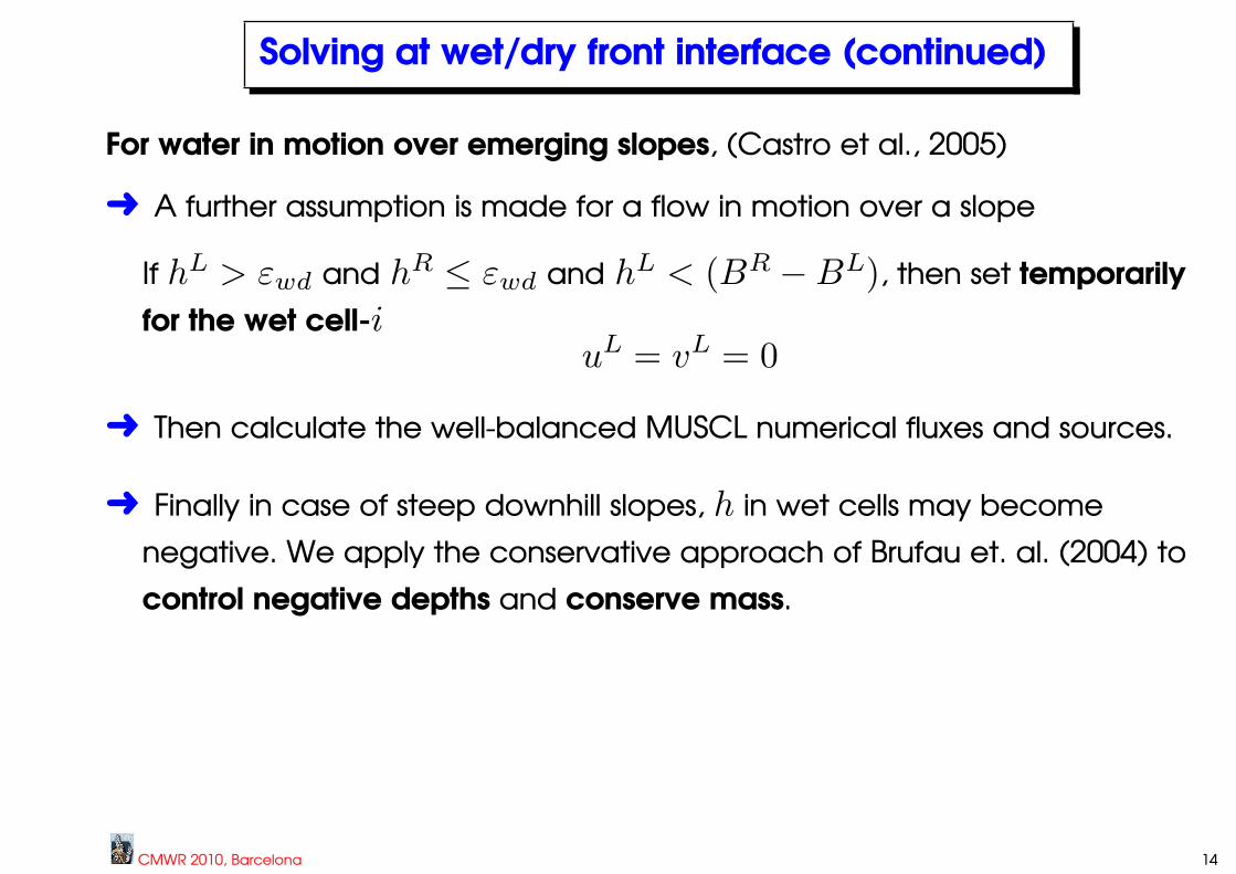
Solving at wet/dry front interface (continued)
For water in motion over emerging slopes, (Castro et al., 2005)
Ü A further assumption is made for a flow in motion over a slope
CMWR 2010, Barcelona 14
Solving at wet/dry front interface (continued)
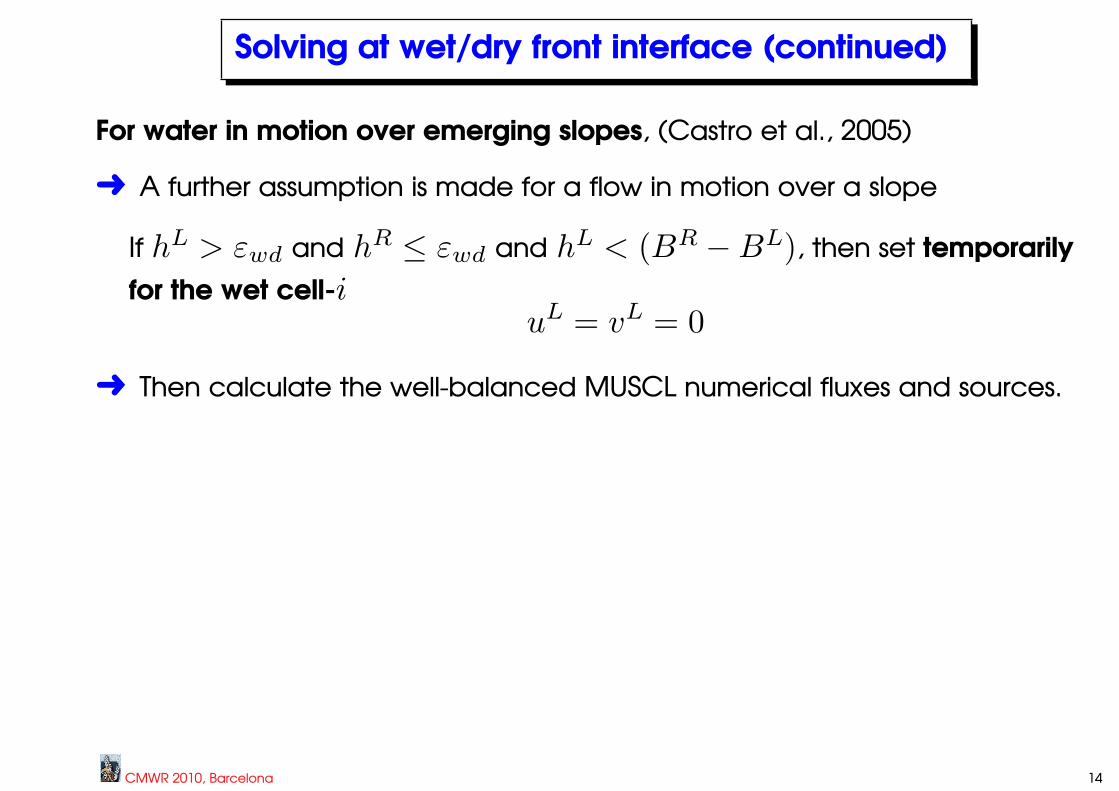
For water in motion over emerging slopes, (Castro et al., 2005)
Ü A further assumption is made for a flow in motion over a slope
If hL > εwd and hR ≤ εwd and hL < (BR −BL), then set temporarily
for the wet cell-iuL = vL = 0
Ü Then calculate the well-balanced MUSCL numerical fluxes and sources.
CMWR 2010, Barcelona 14
Solving at wet/dry front interface (continued)
For water in motion over emerging slopes, (Castro et al., 2005)
Ü A further assumption is made for a flow in motion over a slope
If hL > εwd and hR ≤ εwd and hL < (BR −BL), then set temporarily
for the wet cell-iuL = vL = 0
Ü Then calculate the well-balanced MUSCL numerical fluxes and sources.
Ü Finally in case of steep downhill slopes, h in wet cells may become
negative. We apply the conservative approach of Brufau et. al. (2004) to
control negative depths and conserve mass.
CMWR 2010, Barcelona 14
Other implementation details:• Dry cell identification: use a wet/dry tolerance parameter εwd depending on grid
characteristics (Ricchiuto and Bollerman, 2009).
εwd =
(hN
Lref
)2
CMWR 2010, Barcelona 15

Other implementation details:• Dry cell identification: use a wet/dry tolerance parameter εwd depending on grid
characteristics (Ricchiuto and Bollerman, 2009).
εwd =
(hN
Lref
)2
• Boundary conditions: use the theory of characteristics for: weak formulation for the NVFV
scheme and ghost cells for CCFV scheme.
• Apply a four stage 2nd order Runge-Kutta scheme, due to its enhanced stability region,
under the CFL condition
∆tn = CFL ·mini
(Ri(√
u2 + v2 + c)i
).
• Semi-implicit or implicit treatment for the friction source term within each cell following
Brufau et al., 2004 and Serrano-Pacheco et al., 2009.
CMWR 2010, Barcelona 15
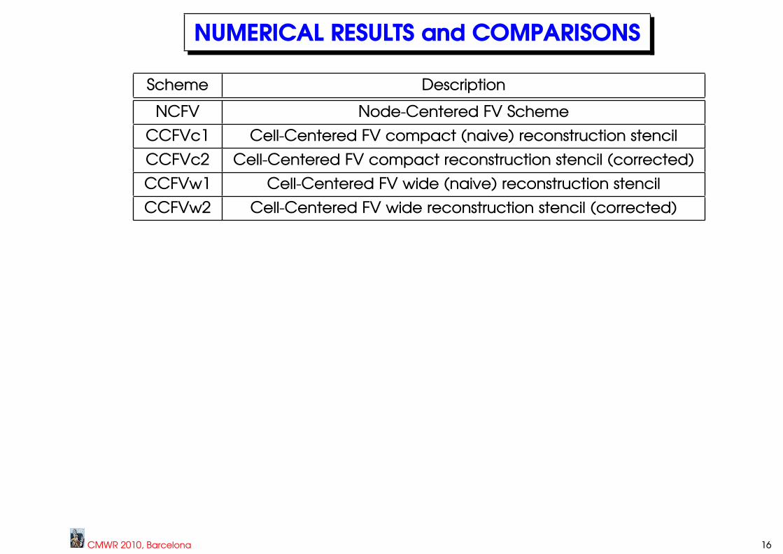
NUMERICAL RESULTS and COMPARISONS
Scheme Description
NCFV Node-Centered FV Scheme
CCFVc1 Cell-Centered FV compact (naive) reconstruction stencil
CCFVc2 Cell-Centered FV compact reconstruction stencil (corrected)
CCFVw1 Cell-Centered FV wide (naive) reconstruction stencil
CCFVw2 Cell-Centered FV wide reconstruction stencil (corrected)
CMWR 2010, Barcelona 16
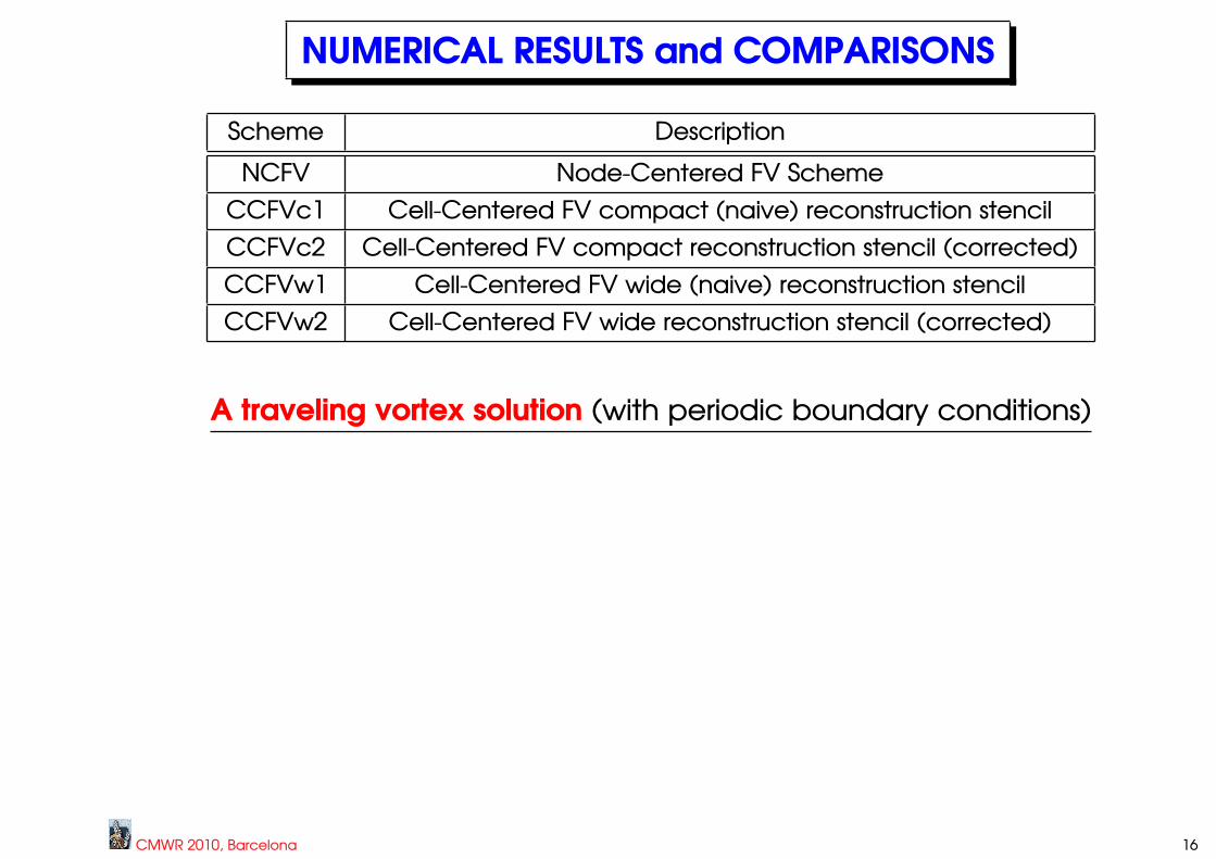
NUMERICAL RESULTS and COMPARISONS
Scheme Description
NCFV Node-Centered FV Scheme
CCFVc1 Cell-Centered FV compact (naive) reconstruction stencil
CCFVc2 Cell-Centered FV compact reconstruction stencil (corrected)
CCFVw1 Cell-Centered FV wide (naive) reconstruction stencil
CCFVw2 Cell-Centered FV wide reconstruction stencil (corrected)
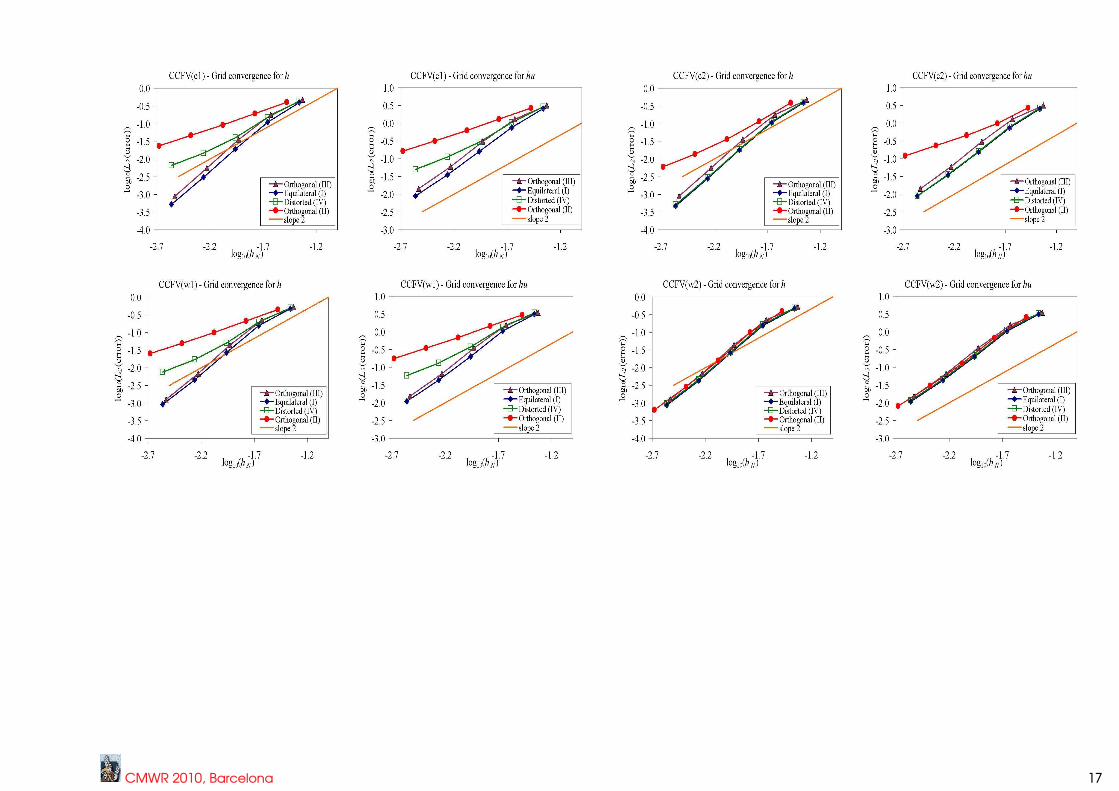
A traveling vortex solution (with periodic boundary conditions)
CMWR 2010, Barcelona 16
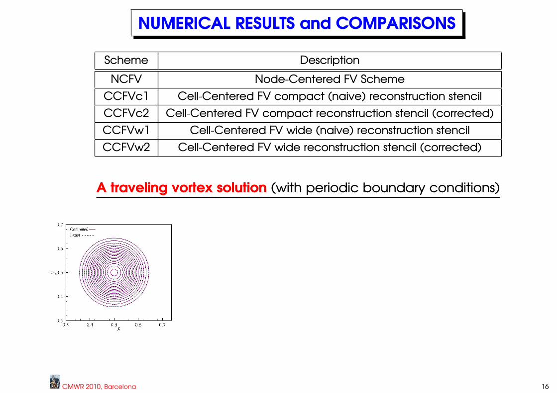
NUMERICAL RESULTS and COMPARISONS
Scheme Description
NCFV Node-Centered FV Scheme
CCFVc1 Cell-Centered FV compact (naive) reconstruction stencil
CCFVc2 Cell-Centered FV compact reconstruction stencil (corrected)
CCFVw1 Cell-Centered FV wide (naive) reconstruction stencil
CCFVw2 Cell-Centered FV wide reconstruction stencil (corrected)
A traveling vortex solution (with periodic boundary conditions)
CMWR 2010, Barcelona 16

CMWR 2010, Barcelona 17
CMWR 2010, Barcelona 17
CMWR 2010, Barcelona 17
CMWR 2010, Barcelona 17
CMWR 2010, Barcelona 17

CMWR 2010, Barcelona 17

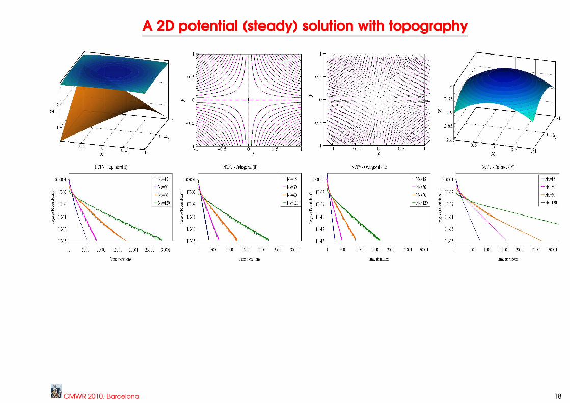
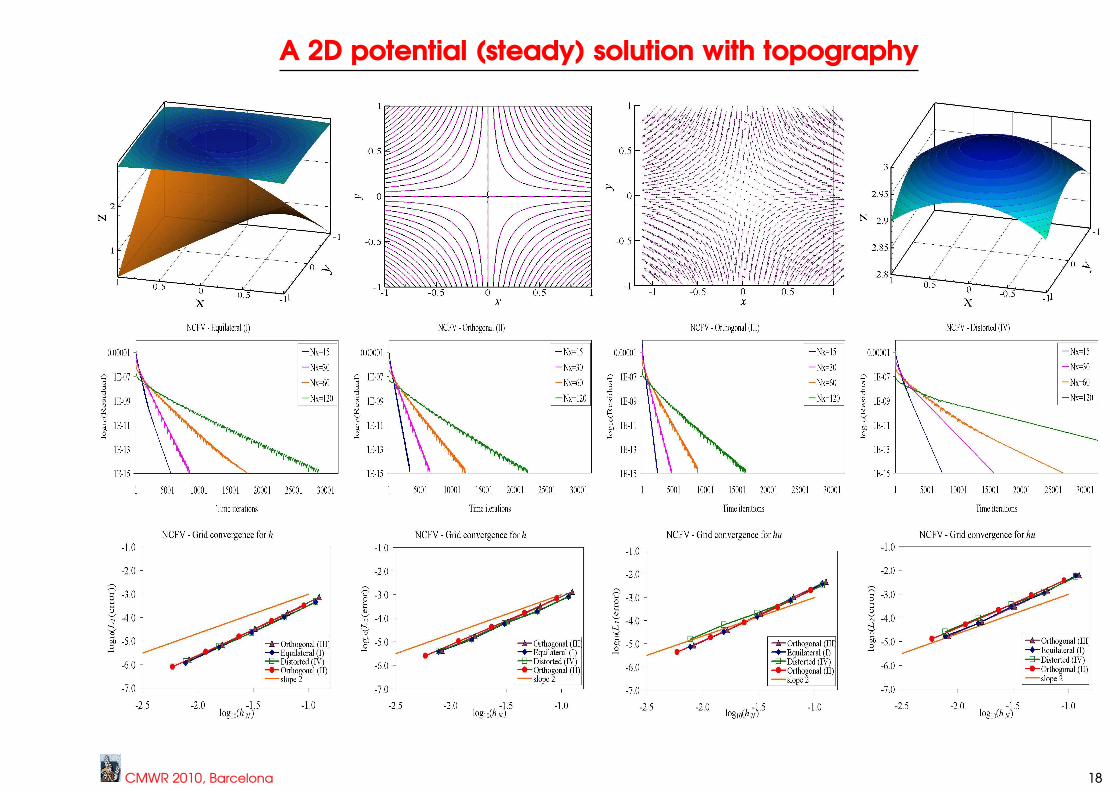
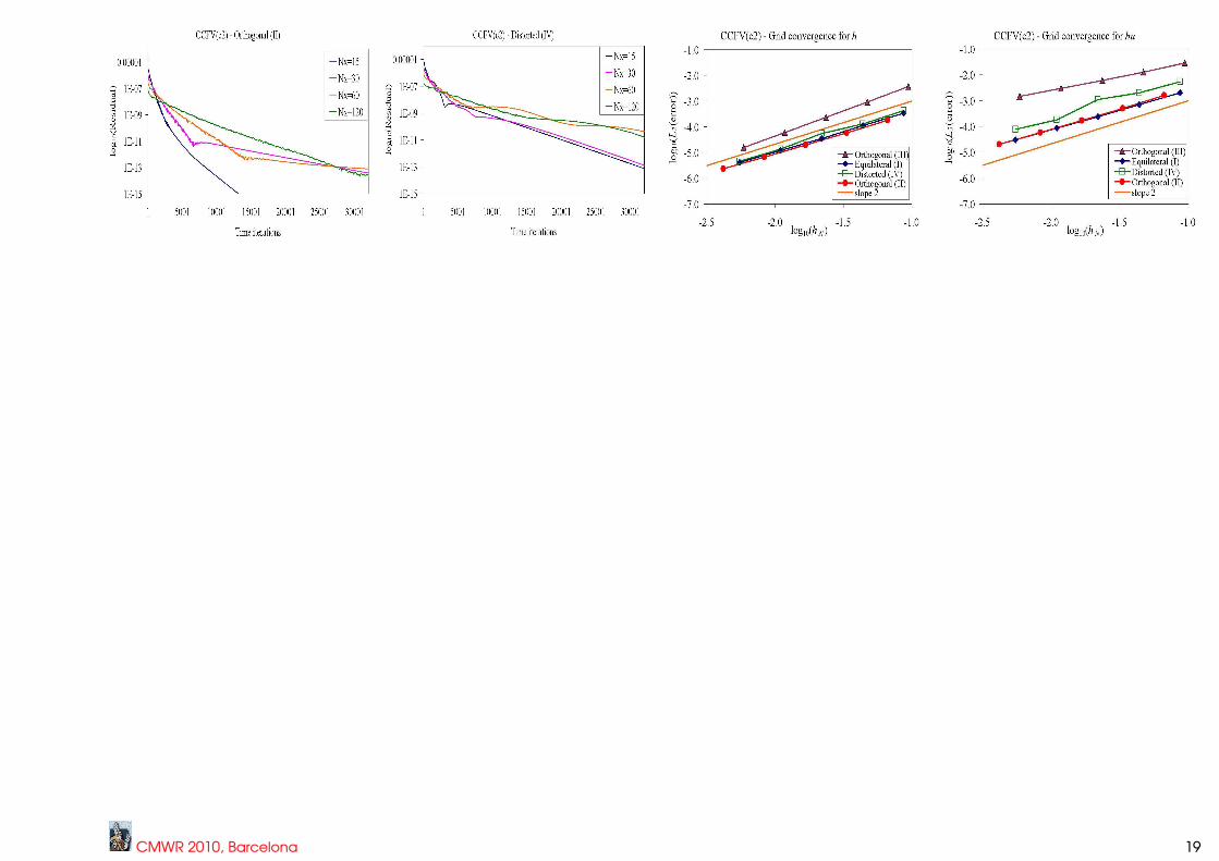
A 2D potential (steady) solution with topography
CMWR 2010, Barcelona 18
A 2D potential (steady) solution with topography
CMWR 2010, Barcelona 18
A 2D potential (steady) solution with topography
CMWR 2010, Barcelona 18
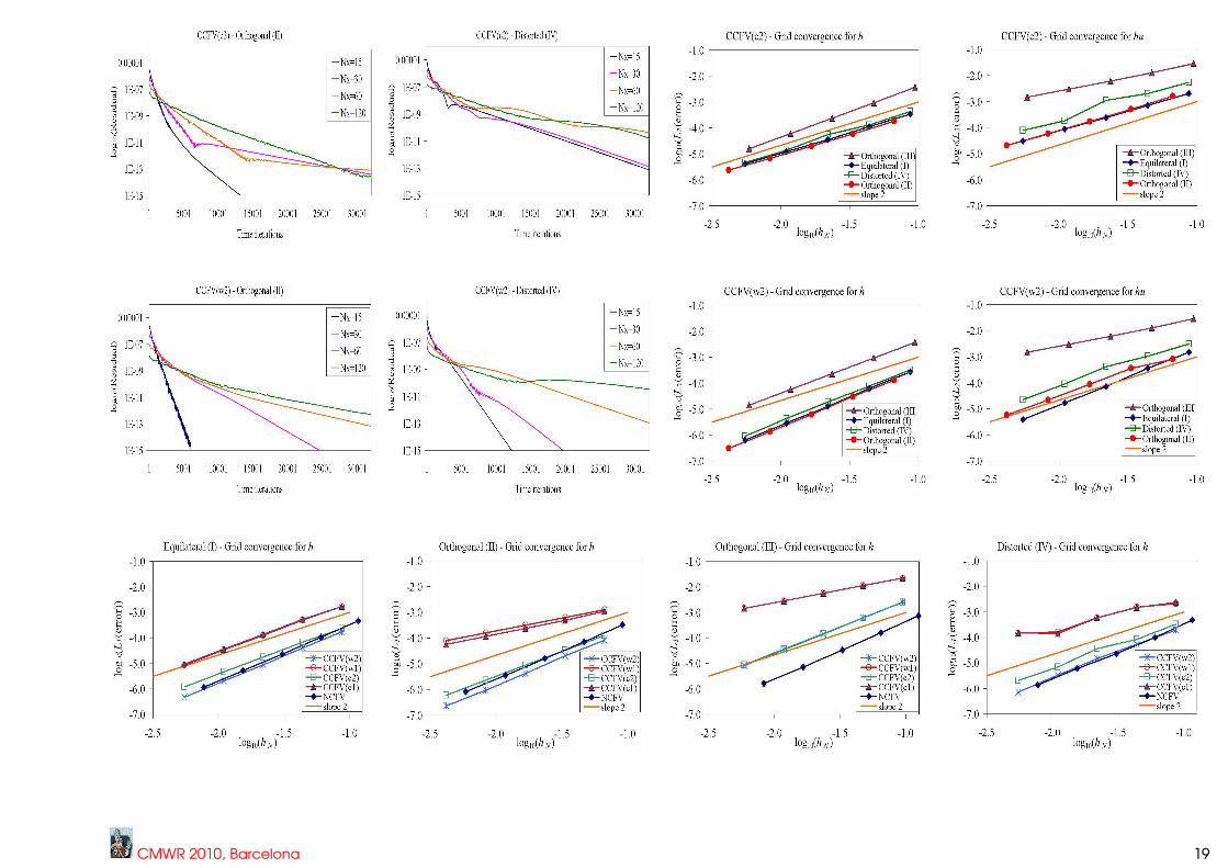
CMWR 2010, Barcelona 19

CMWR 2010, Barcelona 19
CMWR 2010, Barcelona 19
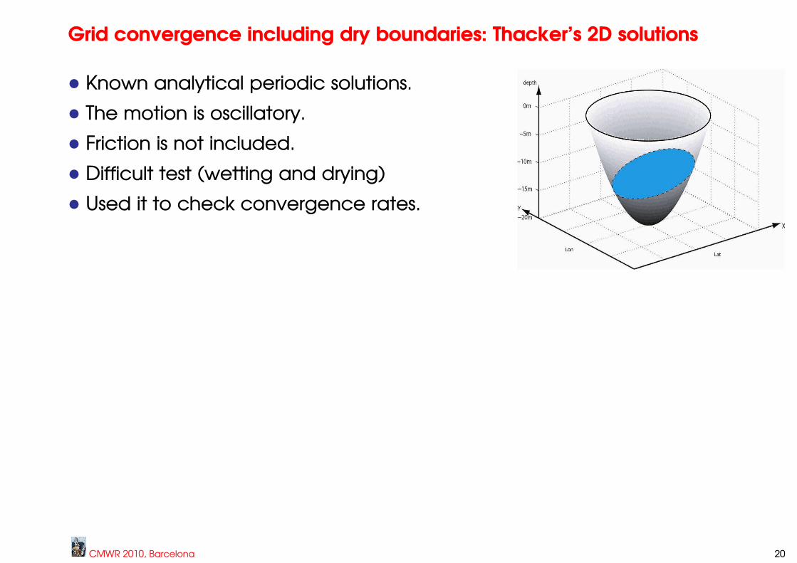
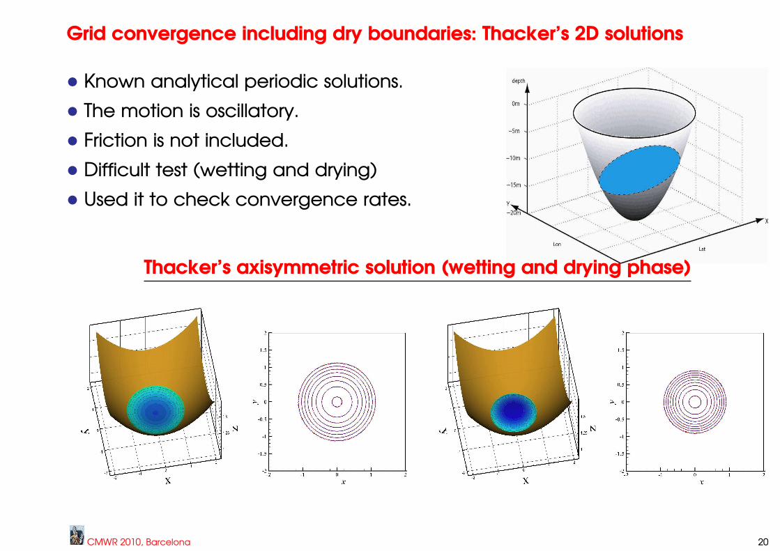
Grid convergence including dry boundaries: Thacker’s 2D solutions
• Known analytical periodic solutions.
• The motion is oscillatory.
• Friction is not included.
• Difficult test (wetting and drying)
• Used it to check convergence rates.
CMWR 2010, Barcelona 20
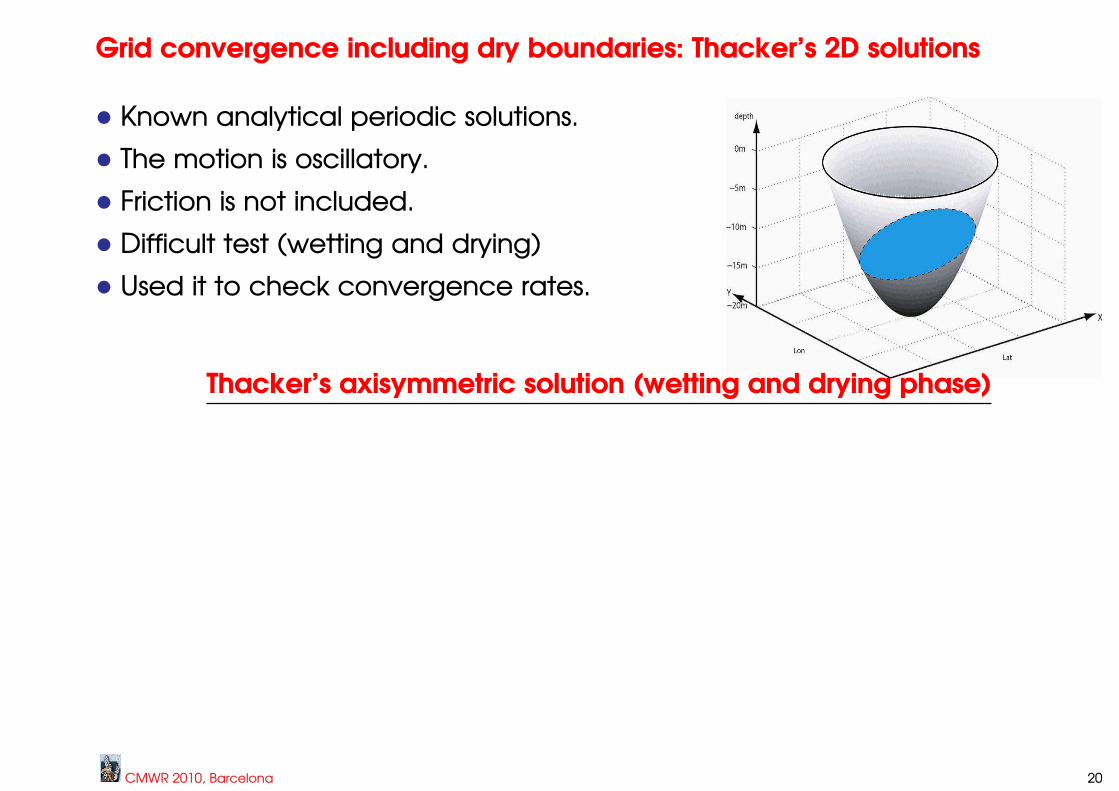
Grid convergence including dry boundaries: Thacker’s 2D solutions
• Known analytical periodic solutions.
• The motion is oscillatory.
• Friction is not included.
• Difficult test (wetting and drying)
• Used it to check convergence rates.
Thacker’s axisymmetric solution (wetting and drying phase)
CMWR 2010, Barcelona 20
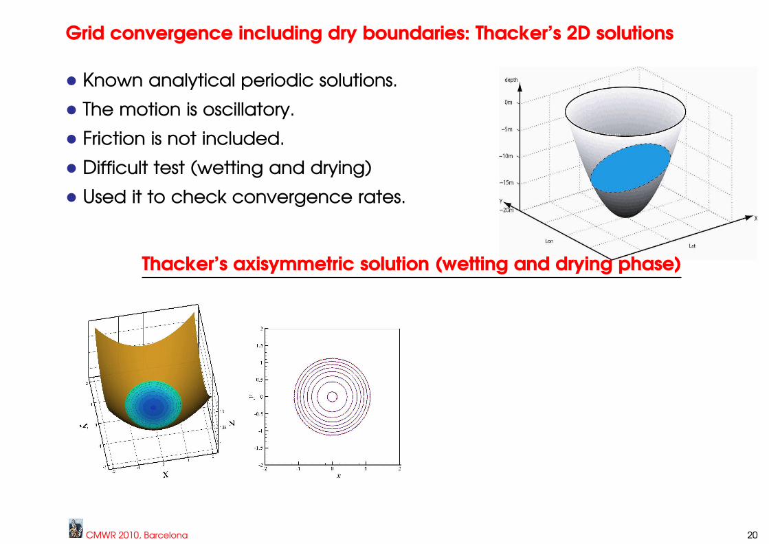
Grid convergence including dry boundaries: Thacker’s 2D solutions
• Known analytical periodic solutions.
• The motion is oscillatory.
• Friction is not included.
• Difficult test (wetting and drying)
• Used it to check convergence rates.
Thacker’s axisymmetric solution (wetting and drying phase)
CMWR 2010, Barcelona 20
CMWR 2010, Barcelona 21

CMWR 2010, Barcelona 21
CMWR 2010, Barcelona 21
CMWR 2010, Barcelona 22

CMWR 2010, Barcelona 22

CMWR 2010, Barcelona 22
The Maplasset dam-break test case (EDF grid, CFL=0.9, nm = 0.033)
CMWR 2010, Barcelona 23
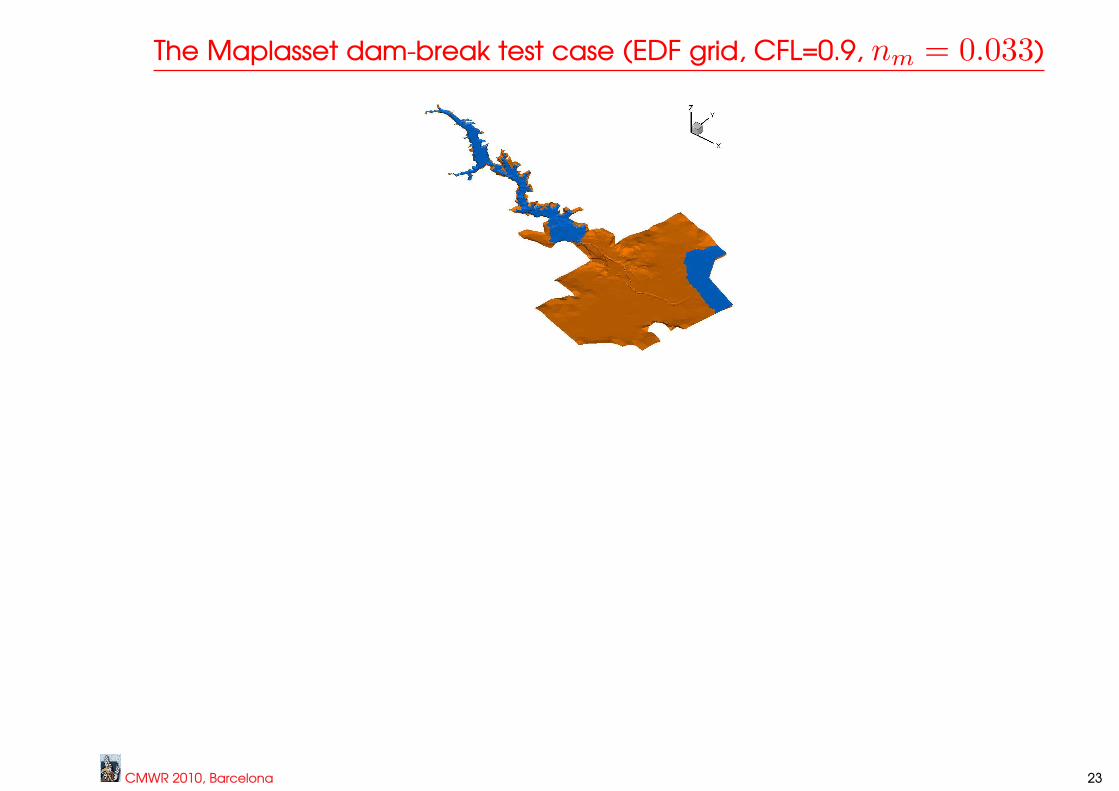
The Maplasset dam-break test case (EDF grid, CFL=0.9, nm = 0.033)
CMWR 2010, Barcelona 23
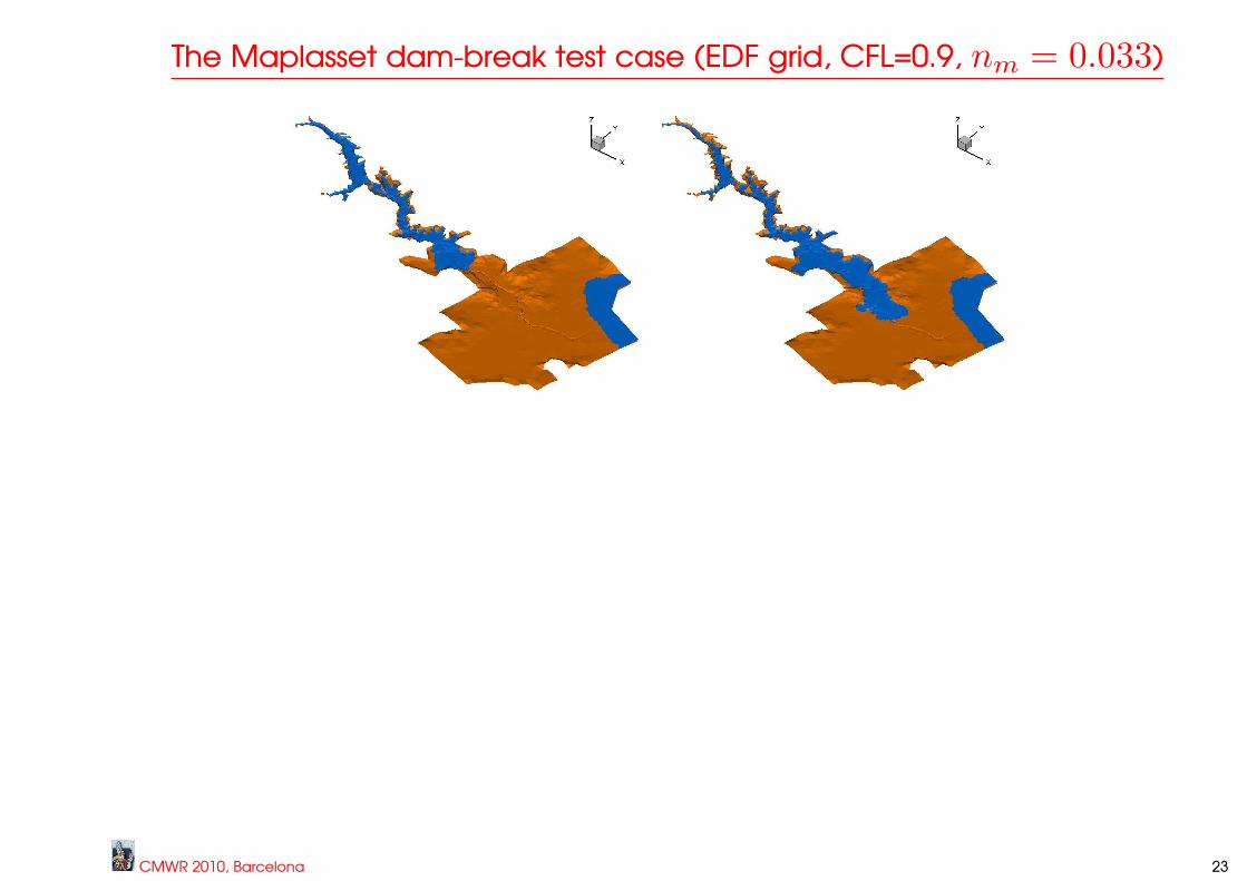
The Maplasset dam-break test case (EDF grid, CFL=0.9, nm = 0.033)
CMWR 2010, Barcelona 23

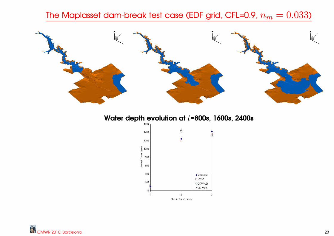
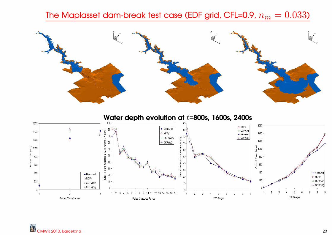
The Maplasset dam-break test case (EDF grid, CFL=0.9, nm = 0.033)
Water depth evolution at t=800s, 1600s, 2400s
CMWR 2010, Barcelona 23
The Maplasset dam-break test case (EDF grid, CFL=0.9, nm = 0.033)
Water depth evolution at t=800s, 1600s, 2400s
CMWR 2010, Barcelona 23

The Maplasset dam-break test case (EDF grid, CFL=0.9, nm = 0.033)
Water depth evolution at t=800s, 1600s, 2400s
CMWR 2010, Barcelona 23

The Maplasset dam-break test case (EDF grid, CFL=0.9, nm = 0.033)
Water depth evolution at t=800s, 1600s, 2400s
CMWR 2010, Barcelona 23
The Maplasset dam-break test case (EDF grid, CFL=0.9, nm = 0.033)
Water depth evolution at t=800s, 1600s, 2400s
CMWR 2010, Barcelona 23

CONCLUSIONS
• The NCFV scheme exhibited identical convergence behavior on all grids.
CMWR 2010, Barcelona 24

CONCLUSIONS
• The NCFV scheme exhibited identical convergence behavior on all grids.
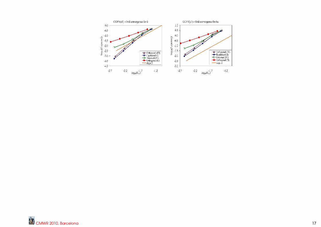
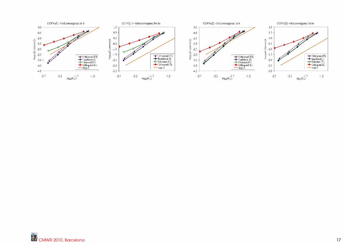
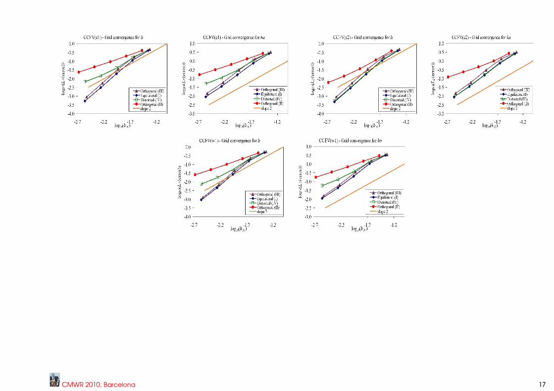
• For the CCFV approach different convergence behavior is exhibited (with
an order reduction) for grids where the center of the face does not coincide
with the reconstruction location.
CMWR 2010, Barcelona 24
CONCLUSIONS
• The NCFV scheme exhibited identical convergence behavior on all grids.
• For the CCFV approach different convergence behavior is exhibited (with
an order reduction) for grids where the center of the face does not coincide
with the reconstruction location.
• The proposed correction for the reconstruction values remedies the problem (for both the
compact and wide stencil G-G gradient computations)
• For the wide stencil similar consistent convergence behavior to the NCFV is exhibited
• Convergence to steady-state solutions is greatly improved.
• The effect of the grid’s geometry at the boundary can lead to order
reduction for the CCFV schemes (if the the center of the face does not
coincide with the reconstruction location), even for good quality grids
• Results with the wide stencil CCFV scheme exhibited, in general, better accuracy.
• Both FV approaches to wetting and drying situations lead to order reduction
but this drop is moderate and within acceptable limits
• Important differences observed between the wetting and drying phase, with the results in
CMWR 2010, Barcelona 24
the drying phase being of reduced accuracy for the velocity computations
CMWR 2010, Barcelona 25
the drying phase being of reduced accuracy for the velocity computations
• For the friction treatment an order reduction for the velocity components
was observed proportional to the implicitness introduced to the numerical
treatment
CMWR 2010, Barcelona 25
the drying phase being of reduced accuracy for the velocity computations
• For the friction treatment an order reduction for the velocity components
was observed proportional to the implicitness introduced to the numerical
treatment
• For the Malpasset case, all formulations produced results close to field
measurements, but with the NCFV scheme using half the degrees of freedom
of the CCFV ones.
CMWR 2010, Barcelona 25

the drying phase being of reduced accuracy for the velocity computations
• For the friction treatment an order reduction for the velocity components
was observed proportional to the implicitness introduced to the numerical
treatment
• For the Malpasset case, all formulations produced results close to field
measurements, but with the NCFV scheme using half the degrees of freedom
of the CCFV ones.
References
• A.I. Delis, I.K. Nikolos and M.Kazolea, "Performance and comparison of cell-centered and
node-centered unstructured finite volume discretizations for shallow water free surface flows",
Archives of Computational Methods in Engineering, (accepted).
• I.K. Nikolos and A.I. Delis, "An unstructured nod-centered finite volume scheme for shallow
water flows with wet/dry front over complex topography", Comput. Methods Appl. Mech.
Engrg., 198:3723, 2009.
THANK YOU FOR YOUR ATTENTION!
CMWR 2010, Barcelona 25
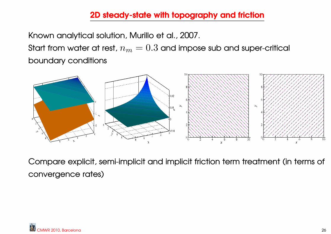
2D steady-state with topography and friction
Known analytical solution, Murillo et al., 2007.
Start from water at rest, nm = 0.3 and impose sub and super-critical
boundary conditions
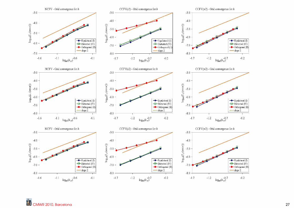
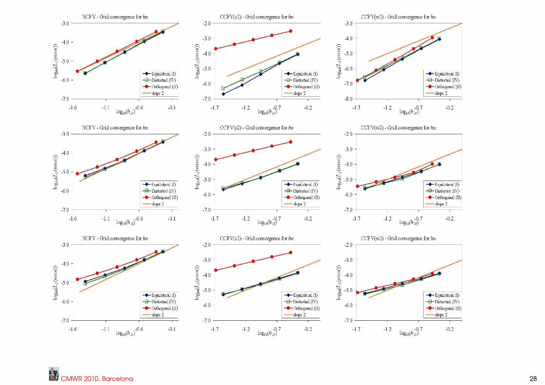
Compare explicit, semi-implicit and implicit friction term treatment (in terms of
convergence rates)
CMWR 2010, Barcelona 26
CMWR 2010, Barcelona 27
CMWR 2010, Barcelona 28