Centre for Strategic Educational Research DPU, Aarhus University

Working Paper Series

CSER WP No. 0003

Comparing Regression Coefficients Between Models using Logit and Probit: A New MethodAf Kristian Bernt Karlson, Anders Holm, and Richard Breen,

August 12, 2010

Comparing Regression Coefficients Between Models using Logit and Probit:A New MethodKristian Bernt Karlson*, Anders Holm**, and Richard Breen***This version: August 12, 2010

Running head: Comparing logit and probit regression coefficients

AbstractLogit and probit models are widely used in empirical sociological research. However, the widespread practice of comparing the coefficients of a given variable across differently specified models does not warrant the same interpretation in logits and probits as in linear regression. Unlike in linear models, the change in the coefficient of the variable of interest cannot be straightforwardly attributed to the inclusion of confounding variables. The reason for this is that the variance of the underlying latent variable is not identified and will differ between models. We refer to this as the problem of rescaling. We propose a solution that allows researchers to assess the influence of confounding relative to the influence of rescaling, and we develop a test statistic that allows researchers to assess the statistical significance of both confounding and rescaling. We also show why y-standardized coefficients and average partial effects are not suitable for comparing coefficients acrossmodels. We present examples of the application of our method using simulated data and data from the Na-tional Educational Longitudinal Survey.

Acknowledgements: We thank Mads Meier Jæger, Robert Mare, and participants at theRC28 conference at Yale 2009 for very helpful comments.

* Centre for Strategic Educational Research, Danish School of Education, University of Education, Denmark, email: kbk@dpu.dk.** Centre for Strategic Educational Research, Danish School of Education, University of Education: aholm@dpu.dk.*** Center for Research on Inequality and the Life Course, Department of Sociology, Yale University, email: richard.breen@yale.edu. Total words: 9480 words (including all text, notes, and references) 4 tables 1 appendix

2

Comparing Regression Coefficients Between Models using Logit and Probit:

A New Method

Introduction

Nonlinear probability models such as binary logit and probit models are widely used in

quantitative sociological research. One of their most common applications is to estimate the

effect of a particular variable of interest on a binary outcome when potentially confounding

variables are controlled. Interest in such genuine or “true” coefficients has a long history in

the social sciences and is usually associated with the elaboration procedure in cross-

tabulation suggested by Lazarsfeld (1955, 1958; Kendall and Lazarsfeld 1950; cf. Simon

1954 for partial product moment correlations). Nevertheless, controlled logit or probit

coefficients do not have the same straightforward interpretation as controlled coefficients in

linear regression. In fact, comparing uncontrolled and controlled coefficients across nested

logit models is not directly feasible, but this appears to have gone unrecognized in much

applied social research, despite an early statement of the problem by Winship and Mare

(1984).

In this paper we offer a solution. We develop a method that allows unbiased

comparisons of logit or probit coefficients of the same variable (x) across nested models

successively including control variables (z). The method decomposes the difference in the

logit or probit coefficient of x between a model excluding z and a model including z, into a

part attributable to confounding (i.e., the part mediated or explained by z) and a part

attributable to rescaling of the coefficient of x. Our method is general because it extends all

the decomposition features of linear models to logit and probit models. In contrast to the

method of y-standardization (Winship and Mare 1984; cf. Long 1997), our method is an

3

analytical solution and it does not depend on the predicted index of the logit or the probit.

Moreover, contrary to popular belief, we prove that average partial effects (as defined by

Wooldridge 2002) can be highly sensitive to rescaling. However, casting average partial

effects in the framework developed in this paper solves the problem created by rescaling

and thereby provides researchers with a more interpretable effect measure than

conventional logit or probit coefficients.

We focus on models for binary outcomes, in particular the logit model, but

our approach applies equally to other nonlinear models for nominal or ordinal outcomes.

We proceed as follows. First, we present the problem of comparing coefficients across

nested logit or probit models. Second, we formally describe the rescaling issue and show

how to assess the relative magnitude of confounding relative to rescaling. We also develop

test statistics that enable formal tests of confounding and rescaling. Third, we show that our

method is preferred over y-standardization and average partial effects. Fourth, we apply our

method to simulated data and to data from the National Educational Longitudinal Survey.

We conclude with a discussion of the wider consequences for current sociological research.

Comparing coefficients across logit and probit models

In linear regression, the concept of controlling for possible confounding variables is well

understood and has great practical value. Researchers often want to assess the effect of a

particular variable on some dependent variable net of one or more confounding variables. A

general consequence of this feature is that researchers can compare controlled (partial)

coefficients with uncontrolled (gross) coefficients, that is, compare coefficients across same

sample nested models. For example, a researcher might want to assess how much the effect

of years of education on log annual income changes when holding constant academic

4

ability and gender. In this case the researcher would compare the uncontrolled coefficient

for years of education with its counterpart controlling for ability and gender. The difference

between the two coefficients reflects the degree to which the impact of years of education is

mediated or confounded by ability and gender.1 This kind of design is straightforward

within the OLS modeling framework and is probably one of the most widespread practices

in empirical social research (Clogg, Petkova, and Haritou 1995).

In logit and probit models, however, uncontrolled and controlled coefficients

can differ not only because of confounding but also because of a rescaling of the model. In

this case the size of the estimated coefficient of the variable of interest depends on the error

variance of the model and, consequently, on which other variables are in the model.

Including a control variable, z, in a logit or probit model will alter the coefficient of x

whether or not z is correlated with x, because, if z explains any of the variation in the

dependent variable, its inclusion will reduce the error variance of the model. Consequently,

logit or probit coefficients from different nested models are not measured on the same scale

and are therefore not directly comparable. This comes about because, in nonlinear

probability models, the error variance is not independently identified and is fixed at a given

value (Cramer 2003:22).2 This identification restriction is well known in the literature on

limited dependent variable models (Yatchew and Griliches 1985, Long 1997; Powers and

Xie 2000; Cramer 2003; Winship and Mare 1984; Maddala 1983; Amemiya 1975; Agresti

2002), but the consequences of rescaling for the interpretation of logit or probit coefficients

1 We use ‘confounding’ as a general term to cover all cases in which additional variables, z, are correlated with the original explanatory variable, x, and also affect the dependent variable, y. This includes cases where the additional variables are believed to ‘mediate’ the original relationship x and y. In terms of path analyses, the part of the x-y relationship mediated or confounded by z is the indirect effect. 2 This identification restriction holds for all models in which the error variance is a direct function of the mean (McCullagh and Nelder 1989). In the linear regression model, the mean and error variance are modeled independently.

5

are far from fully recognized in applied social research (for similar statements, see Allison

1999, Hoetker 2004; 2007, Williams 2009, or Mood 2010).

One very important reason why we should be concerned with this problem

arises when we have a policy variable, z, which we believe will mediate the relationship

between x and a binary outcome, y. Typically, we might first use a logit model to regress y

on x to gauge the magnitude of the relationship, and then we might add z as a control to find

out how much of the relationship is mediated via z. This would seem to tell us how much

we could affect the x-y relationship by manipulating z. But, as we show below, in general

such a strategy will tend to underestimate the mediating role of z, increasing the likelihood

of our concluding, incorrectly, that changing z would have little or no impact on the x-y

relationship.

Known solutions to the problem of comparing coefficients across nested logit

or probit models are to use y-standardization (Winship and Mare 1984) or to calculate

average partial effects (Wooldridge 2002). However, as we show, these solutions are

insufficient for dealing with the problem of comparing logit or probit coefficients across

models in a satisfactory manner.

Separating confounding and rescaling

In this section, to set the notation, we first formally show how coefficient rescaling operates

in the logistic regression model.3 After this exposition, we introduce a novel method that

decomposes the change in logit coefficients across nested models into a confounding

component and a rescaling component. We also develop analytical standard errors and t-

3 The results hold equally for probit models.

6

statistics for each component, and point out an unrecognized similarity with a test statistic

provided in Clogg, Petkova, and Haritou (1995) for linear models.

Latent linear formulation of a logit model

Let *y be a continuous latent variable representing the propensity of occurrence of some

sociologically interesting response variable (e.g., completing a particular level of education,

committing a crime, or experiencing a divorce). Let x be an explanatory variable of interest

(e.g., parental education, parental criminal behavior, or one’s own educational attainment),

and let z be a set of control variables (e.g., academic ability, mental well being, or number

of children). In this exposition we assume that x and z will be correlated, thereby allowing

for z to confound the x-y* relationship. Omitting individual subscripts and centering x and z

on their respective means (i.e., omitting the intercepts), we follow the notation for linear

models in Clogg, Petkova, and Haritou (1995; cf. Blalock 1979) and specify two latent

variable models:

*RH : , ( )yx Ry x e sd eβ σ= + = (1)

*FH : , ( ) ,yx z yz x Fy x z v sd vβ β σ⋅ ⋅= + + = (2)

HR and HF denote the reduced and full model respectively and we take HF to be the true

model.4 However, an identification problem arises because we cannot observe y*: instead

we observe y, a dichotomized version of the latent propensity such that:

1 if *

0 otherwise,

y y

y

τ= >=

(3)

4 Following Clogg, Petkova, and Haritou (1995) we use the term “full model” to denote the model including controls, while we denote the model without controls the “reduced model”. Since both models cannot be true simultaneously, we hold the full model to be the “true” model, i.e., the model on which we will base our inferences.

7

where τ is a threshold, normally set to zero.5 The expected outcome of this binary indicator

is the probability of choosing 1y = , i.e., ( 1) Pr( 1)E y y= = = . Assuming that the error terms

in (1) and (2) follow a logistic distribution we can write the two latent models in the form

*y x e x uβ β σ= + = + where σ is a scale parameter and where u is a standard logistic

random variable with mean 0 and standard deviation / 3π (Cramer 2003:22; Long

1997:119).6 Using this additional notation and setting0τ = , we obtain the following two

logit models, corresponding to (1) and (2) above:

( )

( )( )

LogitRH :

exp

Pr( 1) Pr * 0 Pr

1 exp

explogit(Pr( 1)) .

1 exp

yx

yx R

yxR

R

yx yxyx

Ryx

x

y y u x

x

b xy b x

b x

ββ σ

βσσ

βσ

= = > = < − = +

= ⇔ = = =+

(4)

and in a similar way we obtain the full model

( )( )

LogitFH :

expPr( 1)

1 exp

logit(Pr( 1))

yx z yz x

yx z yz x

yx z yz xyx z yz x

F F

b x b zy

b x b z

y b x b z x zβ βσ σ

⋅ ⋅

⋅ ⋅

⋅ ⋅⋅ ⋅

+= =

+ +

⇔ = = + = +

(5)

where the residual standard deviations, Rσ and Fσ , are defined in Models HR and HF. We

can immediately see that the coefficients for x from the two models, yxb and yx zb ⋅ , are

influenced not only by whether other variables are included in the model but also by the

magnitude of the residual variance.

5 Whenever the threshold constant is nonzero, it is absorbed in the intercept of the logit model. However, it does not affect the effect estimates. Therefore, we set the threshold to zero in this paper. 6 Had we assumed u to be a standard normal random variable with mean 0 and standard deviation 1, we would have obtained the probit.

8

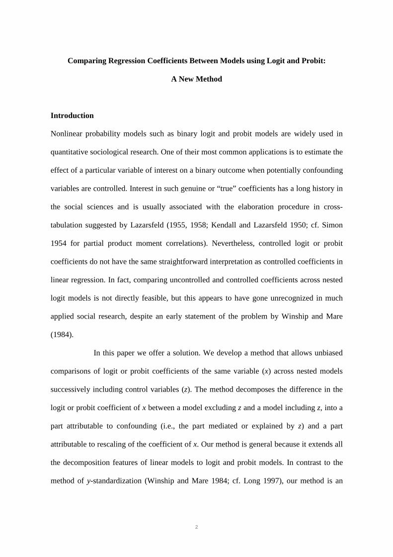
Two sources of change: Confounding and rescaling

From the logit models in (4) and (5) we see that, because we cannot estimate the variance

of *y (i.e., we only observe y as in (3)), a restriction is necessary for identifying the model.

This means that we cannot estimate the regression coefficients of x of the underlying

models in (1) and (2), but only

; yx yx zyx yx z

R F

b bβ βσ σ

⋅⋅= = . (6)

In words, the estimated logit coefficients are equal to the underlying coefficients divided by

the residual standard deviation. Therefore, controlling a variable of interest (x) for a

confounding variable (z) that explains variation in the dependent variable (y) will alter the

coefficient of interest as a result of both confounding and rescaling. Confounding occurs

whenever x and z are correlated and z has an independent effect on y* in the full model.

Rescaling occurs because the model without the confounding variable, z, has a different

residual standard deviation than the model that includes the confounding variable (Rσ as

opposed to Fσ ). Because we explain more residual variation in the full model than in the

reduced model, it holds that R Fσ σ> . The logit coefficients of x are therefore measured on

different scales.7

7 Rescaling will also affect the odds-ratio, i.e., the exponentiated logit coefficient. Because of the simple relation between log-odds-ratios and odds-ratios, this impact is straightforward to show. By odds-ratio we mean the relative probability or odds for the event of interest between two different individuals, i.e., if Y is a binary dependent variable and x and x’ are two different values of an independent variable, then the odds-ratio

is defined as ( 1| ) ( 1| ')

1 ( 1| ) 1 ( 1| ')

P Y X x P Y X x

P Y X x P Y X x

= = = =− = = − = =

and then the log-odds-ratio becomes

( ) ( )( 1| ) ( 1| ')ln ln1 ( 1| ) 1 ( 1| ')P Y X x P Y X x

P Y X x P Y X x= = = =−− = = − = = , which is equal to /xβ σ

if the probability of Y follows a logistic distribution, where *y x eα β σ= + + with *y

being a continuously

9

The solution

When employing the logit model, we are interested in the difference between the

underlying coefficients, yxβ and yx zβ ⋅ in (1) and (2), because this difference is the result of

confounding only (and not rescaling). However, because we only observe the coefficients

in (6) we cannot distinguish between changes in yxb compared to yx zb ⋅ due to rescaling and

to confounding:

.yx yx zyx yx z yx yx z

R F

b bβ β

β βσ σ

⋅⋅ ⋅− = − ≠ − (7)

Moreover, researchers making the naïve comparison in (7) will generally underestimate the

role played by confounding, because R Fσ σ> . In certain circumstances, rescaling may

counteract confounding such that the last difference in (7) is zero, which may lead to the

(incorrect) impression that z does not mediate or confound the effect of x.8 Researchers may

also incorrectly report a suppression effect, which is not a result of confounding (i.e., x and

z are uncorrelated), but only a result of rescaling (i.e., z has an independent effect on y). The

problem stated in (7) may be known by most sociologists specializing in quantitative

methods, though the sociological literature is replete with examples in which the naïve

comparison is made and interpreted as though it reflected pure confounding. Moreover,

although tentative solutions exist, they have not diffused into text books on the topic or into

applied research.

Now we present a method that overcomes the cross-model coefficient

comparability problem. Let zɶ be a set of x-residualized z-variables such that their

correlation with x is zero, i.e., 0xzr =ɶ . In other words, zɶ is the residual from a regression of

distributed latent variable, e being a type I extreme valued distributed residual term, and σ

being a scale

parameter. 8 See the Example section.

10

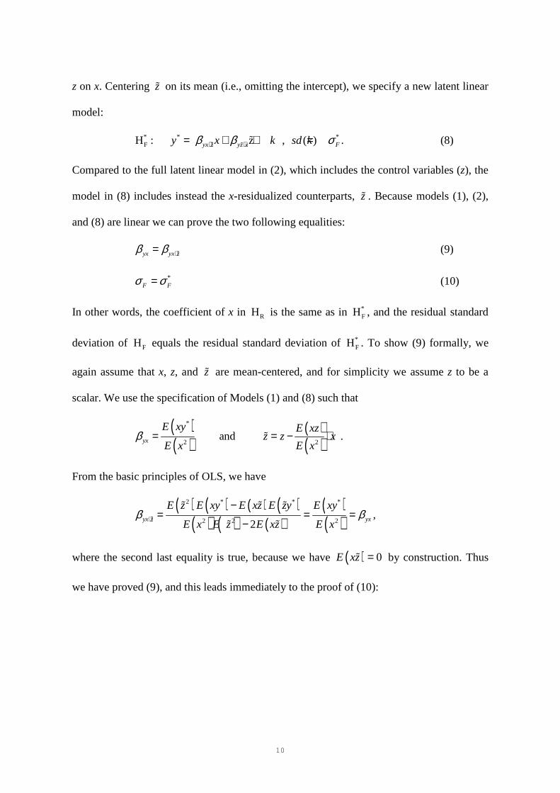
z on x. Centering zɶ on its mean (i.e., omitting the intercept), we specify a new latent linear

model:

* * *FH : z , ( ) .yx z yz x Fy x k sd kβ β σ⋅ ⋅= + + =ɶ ɶ ɶ (8)

Compared to the full latent linear model in (2), which includes the control variables (z), the

model in (8) includes instead the x-residualized counterparts, zɶ . Because models (1), (2),

and (8) are linear we can prove the two following equalities:

yx yx zβ β ⋅= ɶ (9)

*F Fσ σ= (10)

In other words, the coefficient of x in RH is the same as in *FH , and the residual standard

deviation of FH equals the residual standard deviation of *FH . To show (9) formally, we

again assume that x, z, and zɶ are mean-centered, and for simplicity we assume z to be a

scalar. We use the specification of Models (1) and (8) such that

( )( )

( )( )

*

2 2 and yx

E xy E xzz z x

E x E xβ = = − ⋅ɶ .

From the basic principles of OLS, we have

( ) ( ) ( ) ( )( ) ( ) ( )

( )( )

2 * * *

2 2 22yx z yx

E z E xy E xz E zy E xy

E x E z E xz E xβ β⋅

−= = =

−ɶ

ɶ ɶ ɶ

ɶ ɶ,

where the second last equality is true, because we have ( ) 0E xz =ɶ by construction. Thus

we have proved (9), and this leads immediately to the proof of (10):

11

( )( )

( )( )

( )

*

*

2

*

2

*

*

yx z yz x

yx z yz x

yx z yz x yz x

yx z yz x zx yz x

yx z yz x

k y x z

E xzy x z x

E x

E xzy x x z

E x

y x z

y x z

v

β β

β β

β β β

β β θ β

β β

⋅ ⋅

⋅ ⋅

⋅ ⋅ ⋅

⋅ ⋅ ⋅

⋅ ⋅

= − −

= − − − ⋅

= − − ⋅ −

= − − −

= − −=

ɶ ɶ

ɶ

ɶ

ɶ

ɶ

,

where ( )( )2zx

E xz

E xθ = . The relation * y , , k v x z= ∀ implies that *

F Fσ σ= . Thus we have

proved (10). Given the equality in (10), we see that *FH in (8) is a re-parameterization of

FH in (2), i.e., they reflect the same latent linear model.

We now rewrite the latent linear model in (8) into a corresponding logit

model. We employ the same strategy defined by (3), (4), and (5) and obtain the following

model:

Logit*F * *

H : logit(Pr( 1)) .yx z yz xyx z yz x

F F

y b x b z x zβ βσ σ

⋅ ⋅⋅ ⋅= = + = +ɶ ɶ

ɶ ɶ ɶ ɶ (11)

Similar to the linear case, this model is a re-parameterization of LogitFH , i.e., the two models

have the same fit to the data. We may now exploit the equalities in (9) and (10) and the

specifications of the logit models to overcome the comparison issue encountered in (7). In

other words, we can make an unbiased comparison of coefficients of x without and with a

confounding variable, z, in the model. We propose three measures of coefficient change

that hold rescaling constant (i.e., that measure confounding net of rescaling). The first

measure is a difference measure:

*

yx z yx z yx yx z yx yx zyx z yx z

F F F F F

b bβ β β β β βσ σ σ σ σ

⋅ ⋅ ⋅ ⋅⋅ ⋅

−− = − = − =ɶ

ɶ , (12a)

12

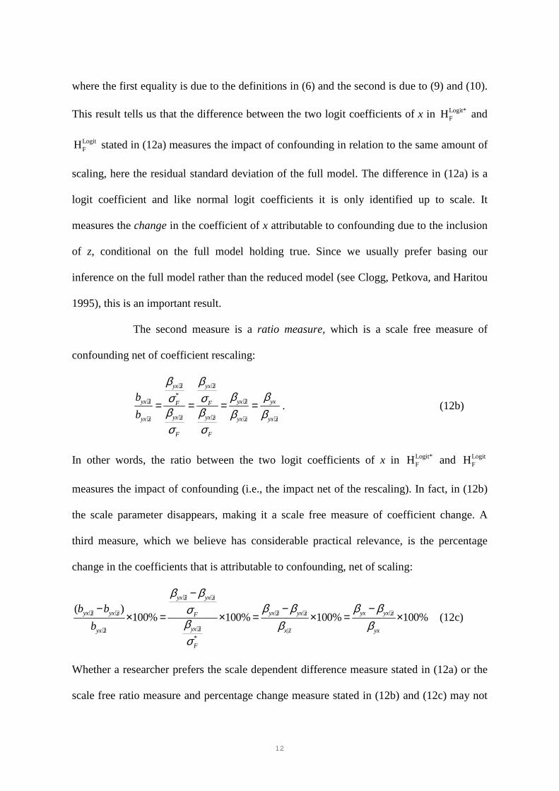
where the first equality is due to the definitions in (6) and the second is due to (9) and (10).

This result tells us that the difference between the two logit coefficients of x in Logit*FH and

LogitFH stated in (12a) measures the impact of confounding in relation to the same amount of

scaling, here the residual standard deviation of the full model. The difference in (12a) is a

logit coefficient and like normal logit coefficients it is only identified up to scale. It

measures the change in the coefficient of x attributable to confounding due to the inclusion

of z, conditional on the full model holding true. Since we usually prefer basing our

inference on the full model rather than the reduced model (see Clogg, Petkova, and Haritou

1995), this is an important result.

The second measure is a ratio measure, which is a scale free measure of

confounding net of coefficient rescaling:

*yx z yx z

yx z yx z yxF F

yx z yx zyx z yx z yx z

F F

b

b

β ββ βσ σ

β β β βσ σ

⋅ ⋅

⋅ ⋅

⋅ ⋅⋅ ⋅ ⋅

= = = =

ɶ ɶ

ɶ ɶ . (12b)

In other words, the ratio between the two logit coefficients of x in Logit*FH and Logit

FH

measures the impact of confounding (i.e., the impact net of the rescaling). In fact, in (12b)

the scale parameter disappears, making it a scale free measure of coefficient change. A

third measure, which we believe has considerable practical relevance, is the percentage

change in the coefficients that is attributable to confounding, net of scaling:

|*

( )100% 100% 100% 100%

yx z yx z

yx z yx z yx z yx z yx yx zF

yx zyx z x z yx

F

b b

b

β ββ β β βσ

β β βσ

⋅ ⋅

⋅ ⋅ ⋅ ⋅ ⋅

⋅⋅

−− − −

× = × = × = ×

ɶ

ɶ ɶ

ɶɶ ɶ

(12c)

Whether a researcher prefers the scale dependent difference measure stated in (12a) or the

scale free ratio measure and percentage change measure stated in (12b) and (12c) may not

13

simply be a matter of choice but should depend on the objective of the research. The

measures have different interpretations. The difference measure in (12a) has the same

properties as a normal logit coefficient and can be treated as such: researchers interested in

the coefficients of the logit model should therefore adopt the difference measure. The ratio

and percentage change measures have a different interpretation, because they are concerned

with the regression coefficients in the latent model. The ratio in (12b) and the percentage

change in (12c) measure change in the underlying partial effects on the latent propensity

rather than in the logit coefficients. We therefore encourage researchers interested in the

underlying partial effects to use these scale free measures.

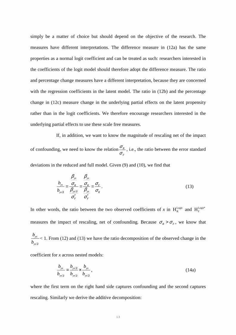
If, in addition, we want to know the magnitude of rescaling net of the impact

of confounding, we need to know the relationRF

σσ

, i.e., the ratio between the error standard

deviations in the reduced and full model. Given (9) and (10), we find that

* *

yx yx

yx FR R

yx z yxyx z R

F F

b

b

β βσσ σ

β β σσ σ

⋅⋅

= = =ɶɶ

. (13)

In other words, the ratio between the two observed coefficients of x in LogitRH and Logit*

FH

measures the impact of rescaling, net of confounding. Because R Fσ σ> , we know that

yx

yx z

b

b ⋅ ɶ

< 1. From (12) and (13) we have the ratio decomposition of the observed change in the

coefficient for x across nested models:

yx yx z yx

yx z yx z yx z

b b b

b b b⋅

⋅ ⋅ ⋅

= ×ɶɶ

, (14a)

where the first term on the right hand side captures confounding and the second captures

rescaling. Similarly we derive the additive decomposition:

14

* *[ ] [ ]yx yx z yx yx z yx z yx z

yx yx z yx yx z yx z yx zR F R F F F

b b b b b bβ β β β β βσ σ σ σ σ σ

⋅ ⋅ ⋅ ⋅⋅ ⋅ ⋅ ⋅− = − = − + − = − + −ɶ ɶ

ɶ , (14b)

where the first term on the right hand side equals rescaling and the second captures

confounding. Notice that the component induced by rescaling is equal to

yx yxyx yx z

R F

b bβ βσ σ⋅− = −ɶ ,

and thus captures the effect, on the logit coefficients, of the change in the residual standard

deviation, holding constant the underlying coefficient.

Rather than looking at the influence of confounders in terms of the rescaling

after adding controls (i.e., using the standard deviation from the full model), a researcher

may want to evaluate this influence in terms of the scaling before adding controls (i.e.,

using the standard deviation from the reduced model). Combining the coefficients of x in

Models (4), (5), and (11), we obtain:

* .yx xy yx zyx z yx z yx z yx

F F F FR R R

β β ββ β β βσ σ σ σσ σ σ

⋅⋅ ⋅ ⋅× = × =ɶ

From these equations we obtain the influence of confounding conditional on the reduced

model holding true:

yx yx z

R

β βσ

⋅− (15)

However, compared to the difference in (12a), the standard error of the difference in (15) is

more difficult to compute. To test the difference in (12a), we calculate the standard error for

the difference between the observed regression coefficients, yx z yx zb b⋅ ⋅−ɶ . This calculation is

straightforward because both coefficients are asymptotically normal (see below). For (15),

however, matters are more difficult because we have to obtain yx z

R

βσ

⋅ as a quotient between

15

several observed quantities. We therefore recommend using (12a) rather than (15) to assess

the influence of confounding. And, to reiterate, in using (12) rather than (15) we are basing

our inferences on the true model.

Two formal tests

We have shown how rescaling operates in the logit model and developed a simple way of

decomposing the change in logit coefficients of the same variable into one part attributable

to confounding and another part attributable to rescaling. However, we also develop two

formal statistical tests that enable researchers to assess whether the change in a coefficient

attributable to confounding is statistically significant and whether rescaling distorts the

results to any statistically significant degree.

For generalized linear models and thus also for logit models, Clogg, Petkova,

and Haritou (1995) show that the standard error of the difference between an uncontrolled

( yxb ) and a controlled (yx zb ⋅ ) logit coefficient is

2 2

2 2 2 2

( ) ( | ) ( | ) 2 ( , )

( | ) ( | ) ( ) ( | ) 2 ( | )

yx yx z yx z F yx F yx z yx

Tyx z F yx R yx R yx R

SE b b SE b H SE b H Cov b b

SE b H SE b H X WX SE b H SE b H

⋅ ⋅ ⋅

⋅

− = + −

= + −. (16)

This somewhat complex expression takes into account the rescaling of the model, because

it involves the variance of yxb conditional on the full model, HF, holding true (HR being the

reduced model). However, while (16) takes into account the rescaling of the standard error

of the difference, it neglects the fact that the difference, yx yx zb b ⋅− , conflates confounding

and rescaling (see (7)). Thus (16) is suitable for coefficient comparisons that mix

confounding and rescaling, but not for comparisons that separate the two sources of change

(see Clogg et al 1995: 1286 Table 5 for an application of their approach to comparing logit

coefficients that does not differentiate the two sources of difference). And since separating

16

confounding and rescaling is precisely our aim, we derive the expression for the standard

error of the difference between the standardardized (i.e. net of rescaling) coefficients. This

is given by

2 2( ) ( ) ( ) 2 ( , )yx z yx zyx z yx z yx z yx z yx z yx z

F

SE b b SE SE b SE b Cov b bβ β

σ⋅ ⋅

⋅ ⋅ ⋅ ⋅ ⋅ ⋅

− − = = + −

ɶ

ɶ ɶ ɶ . (17)

This quantity is easily obtained with standard statistical software.9 We can use (17) to test

the hypothesis of whether change in the logit coefficient attributable to confounding, net of

rescaling, is statistically significant via the test statistic, ZC, (where the subscript C denotes

confounding) which, in large samples, will be normally distributed:

),(2)()( ~..2

~.2

.

.~.

zyxzyxzyxzyx

zyxzyxC

bbCovbSEbSE

bbZ

−+

−= (18)|

In other words, the statistic enables a direct test of the change in the logit coefficients that is

attributable to confounding, net of rescaling.

In passing, we note that, whenever z is a single variable (and not a set of

variables), the Z-statistic for the difference in (12a) equals the Z-statistic for the effect of z

on y as defined in (5):

( ) ( )( )yz x

C yx z yx z C yz x

yz x

bz b b z b

SE b⋅

⋅ ⋅ ⋅⋅

− = =ɶ (19)

So, in the three-variable scenario (y, x, and z) we do not need to use (18): instead we

evaluate the Z-statistic for the effect of z on y in (5). This property is identical to the one

presented by Clogg et al. (1995) for linear regression coefficients. We prove (19) in the

Appendix.

9 Notice that . .( , )yx z yx zCov b b ɶ is not trivial to derive conditional on the full model holding true (under H0). We

use the method implemented in Stata command suest which returns the standard error of the difference (i.e., the denominator in (18)). suest is based on the derivations of a robust sandwich-type estimator, which stacks the equations and weighs the contributions from each equation (see White 1982). Code and sample data are available from the authors.

17

Researchers may also want to know whether coefficient rescaling is

significant or whether they can reasonably ignore its influence. Because R Fσ σ> we test

the one-sided hypothesis:

0

1

:

:

xy xyxy xy z R F

R F

R F

H b b

H

β βσ σ

σ σσ σ

⋅= ⇔ = ⇔ =

>

ɶ

with the following test statistic, which will be normally distributed in large samples:

),(2)()( ~.2

~.2

~.

zyxyxzyxyx

yxzyxS

bbCovbSEbSE

bbZ

−+

−= (20)

where subscript S denotes scaling.

Comparing our method with other known solutions

Why should researchers prefer our method to the alternatives currently available in

statistical packages? We argue that our method is simpler and more precise. Furthermore, y-

standardization, which was suggested by Winship and Mare (1984; cf. Long 1997; Mood

2010) as a possible solution to the comparison problems created by rescaling, is not as

general or as tractable a method as ours. We also show why average partial effects (APEs)

as defined in Wooldridge (2002) cannot be used for direct comparisons of coefficients

across models without and with confounding control variables. However, combining APEs

with the method developed in this paper provides researchers with easily interpretable

effect decompositions.

18

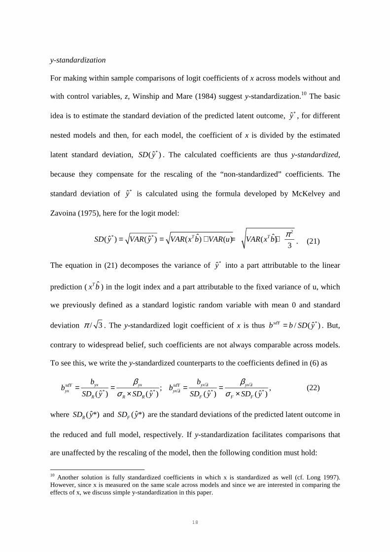
y-standardization

For making within sample comparisons of logit coefficients of x across models without and

with control variables, z, Winship and Mare (1984) suggest y-standardization.10 The basic

idea is to estimate the standard deviation of the predicted latent outcome, *y , for different

nested models and then, for each model, the coefficient of x is divided by the estimated

latent standard deviation, *ˆ( )SD y . The calculated coefficients are thus y-standardized,

because they compensate for the rescaling of the “non-standardized” coefficients. The

standard deviation of *y is calculated using the formula developed by McKelvey and

Zavoina (1975), here for the logit model:

2

* * ˆ ˆˆ ˆ( ) ( ) ( ) ( ) ( )3

T TSD y VAR y VAR x b VAR u VAR x bπ= = + = + . (21)

The equation in (21) decomposes the variance of *y into a part attributable to the linear

prediction ( ˆTx b) in the logit index and a part attributable to the fixed variance of u, which

we previously defined as a standard logistic random variable with mean 0 and standard

deviation / 3π . The y-standardized logit coefficient of x is thus *ˆ/ ( )sdYb b SD y= . But,

contrary to widespread belief, such coefficients are not always comparable across models.

To see this, we write the y-standardized counterparts to the coefficients defined in (6) as

* * * *

; ˆ ˆ ˆ ˆ( ) ( ) ( ) ( )

yx yx yx z yx zsdY sdYyx yx z

R R R F F F

b bb b

SD y SD y SD y SD y

β βσ σ

⋅ ⋅⋅= = = =

× ×, (22)

where ˆ( *)RSD y and ˆ( *)FSD y are the standard deviations of the predicted latent outcome in

the reduced and full model, respectively. If y-standardization facilitates comparisons that

are unaffected by the rescaling of the model, then the following condition must hold:

10 Another solution is fully standardized coefficients in which x is standardized as well (cf. Long 1997). However, since x is measured on the same scale across models and since we are interested in comparing the effects of x, we discuss simple y-standardization in this paper.

19

*

* **

ˆ( )ˆ ˆ( ) ( )

ˆ( )R F

R R F FF R

SD ySD y SD y

SD y

σσ σσ

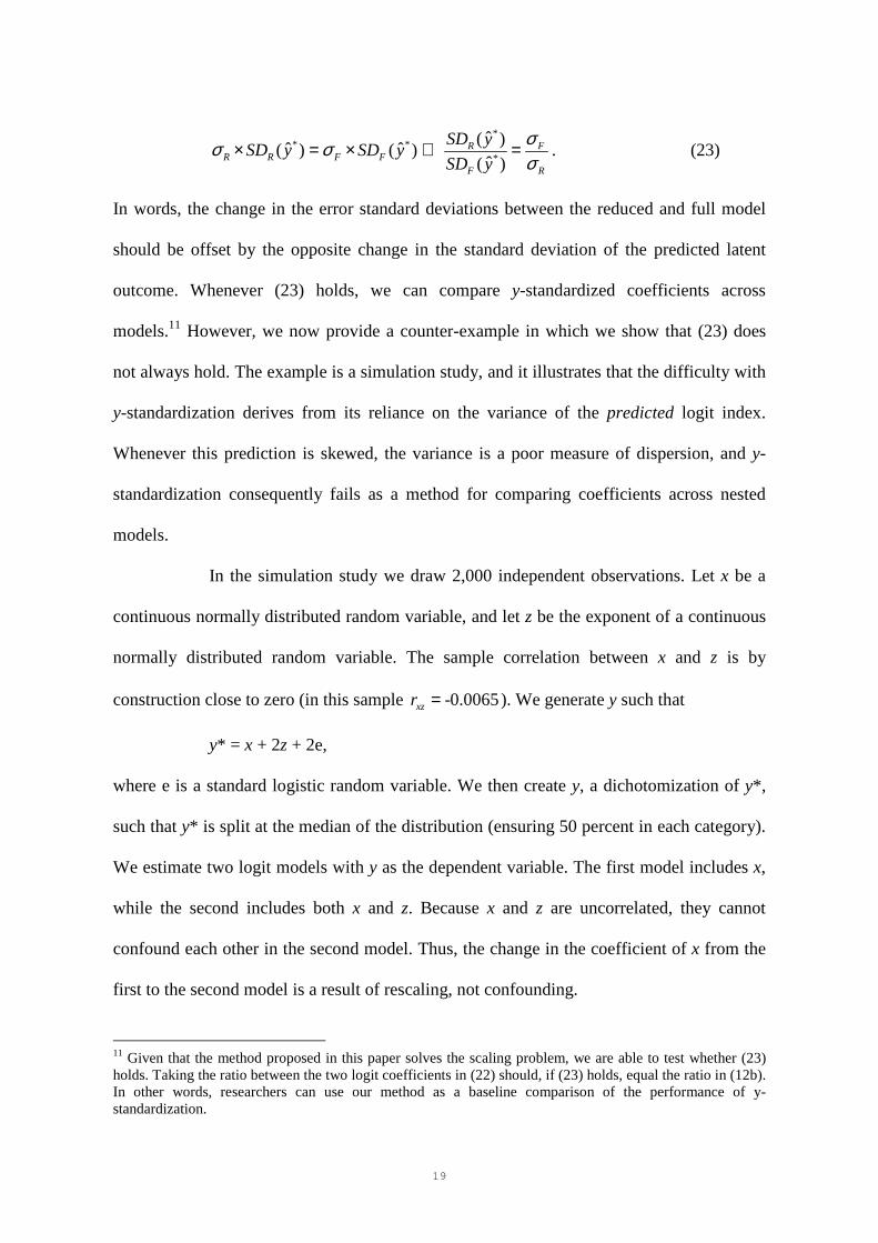
× = × ⇔ = . (23)

In words, the change in the error standard deviations between the reduced and full model

should be offset by the opposite change in the standard deviation of the predicted latent

outcome. Whenever (23) holds, we can compare y-standardized coefficients across

models.11 However, we now provide a counter-example in which we show that (23) does

not always hold. The example is a simulation study, and it illustrates that the difficulty with

y-standardization derives from its reliance on the variance of the predicted logit index.

Whenever this prediction is skewed, the variance is a poor measure of dispersion, and y-

standardization consequently fails as a method for comparing coefficients across nested

models.

In the simulation study we draw 2,000 independent observations. Let x be a

continuous normally distributed random variable, and let z be the exponent of a continuous

normally distributed random variable. The sample correlation between x and z is by

construction close to zero (in this sample -0.0065xzr = ). We generate y such that

y* = x + 2z + 2e,

where e is a standard logistic random variable. We then create y, a dichotomization of y*,

such that y* is split at the median of the distribution (ensuring 50 percent in each category).

We estimate two logit models with y as the dependent variable. The first model includes x,

while the second includes both x and z. Because x and z are uncorrelated, they cannot

confound each other in the second model. Thus, the change in the coefficient of x from the

first to the second model is a result of rescaling, not confounding.

11 Given that the method proposed in this paper solves the scaling problem, we are able to test whether (23) holds. Taking the ratio between the two logit coefficients in (22) should, if (23) holds, equal the ratio in (12b). In other words, researchers can use our method as a baseline comparison of the performance of y-standardization.

20

We report logit coefficients and y-standardized logit coefficients in Table 1.12

A researcher unaware of the rescaling of the logit coefficients of x from Model 1 to Model

2 would erroneously conclude that z is a suppressor of the effect of x on y, because

yx yx zb b ⋅< . yx zb ⋅ is about 30 percent larger than yxb . However, since x and z are uncorrelated,

the inequality only comes about as result of a rescaling of the model. If y-standardization

works satisfactorily, i.e., if the condition in (23) holds, then we would expect it that the

change in the logit coefficients of x between Models 1 and 2 is spurious. The y-standardized

coefficients in the table, however, tell a different story. Here the y-standardized coefficient

of x in Model 1 is larger than the corresponding coefficient in Model 2, thereby “over-

offsetting” the rescaling: sdYyxb

is around 15 percent larger than sdYyx zb ⋅ .

In this case, y-standardization would lead to the conclusion of a reduction in

the effect of x once we control for z. This clearly contradicts a naïve interpretation of the

logit coefficients, which shows an increase of the effect of x. But both are wrong, because

the true change is nil. We have thus shown that y-standardization is not a foolproof

method: it relies on the predicted logit index, and it may lead to incorrect conclusions.

-- TABLE 1 HERE --

Marginal effects and average partial effects

Sociologists are increasingly becoming aware of the scale identification issue in logit and

probit models (see, e.g., Mood 2010). Economists, who have long recognized the problem,

are usually not interested in logit or probit coefficients, but prefer marginal effects (see

Cramer 2003; Wooldridge 2002) or average partial effects, APEs (Wooldridge 2002: 22-4).

12 Calculated with Spost for Stata (Long and Freese 2005).

21

Effects measured on the probability scale are intuitive, both for researchers and policy-

makers. Moreover, even though predicted probabilities are nonlinear and depend on other

variables in the model, they are allegedly “scale free”, thereby escaping the scale

identification issue. We agree that reporting marginal effects and predicted probabilities is a

step forward in making results produced by logit or probit models more interpretable.

Nevertheless, both marginal and average partial effect measures suffer from some

deficiencies that render them unsuitable for comparing coefficients across nested models.

Casting APEs in our framework, however, solves the problem.

Defining marginal effects and average partial effects

In logit and probit models, the marginal effect, ME, of x is the derivative of the predicted

probability with respect to x, given by (when x is continuous13 and differentiable):

ˆ ˆ ˆ(1 )

ˆ ˆ ˆ ˆ(1 ) (1 )dp p p

p p b p pdx

β βσ σ

−= − = − = , (24)

where ˆ Pr( 1| )p y x= = is the predicted probability given x and bβσ

= is the logit

coefficient of x. The ME of x is evaluated at some fixed values of the other explanatory

variables in the model, typically their means. But this implies that whenever we include

control variables in a model we change the set of other variables at whose mean the ME is

evaluated, so introducing indeterminacy into cross-model comparisons. We therefore ignore

MEs in the following discussions, and rather focus on the more general APE.

13 Whenever x is discrete, the ME is the difference(s) in expected probabilities for each discrete category. In this paper, we refer to the continuous case. The discrete case follows directly from these derivations.

22

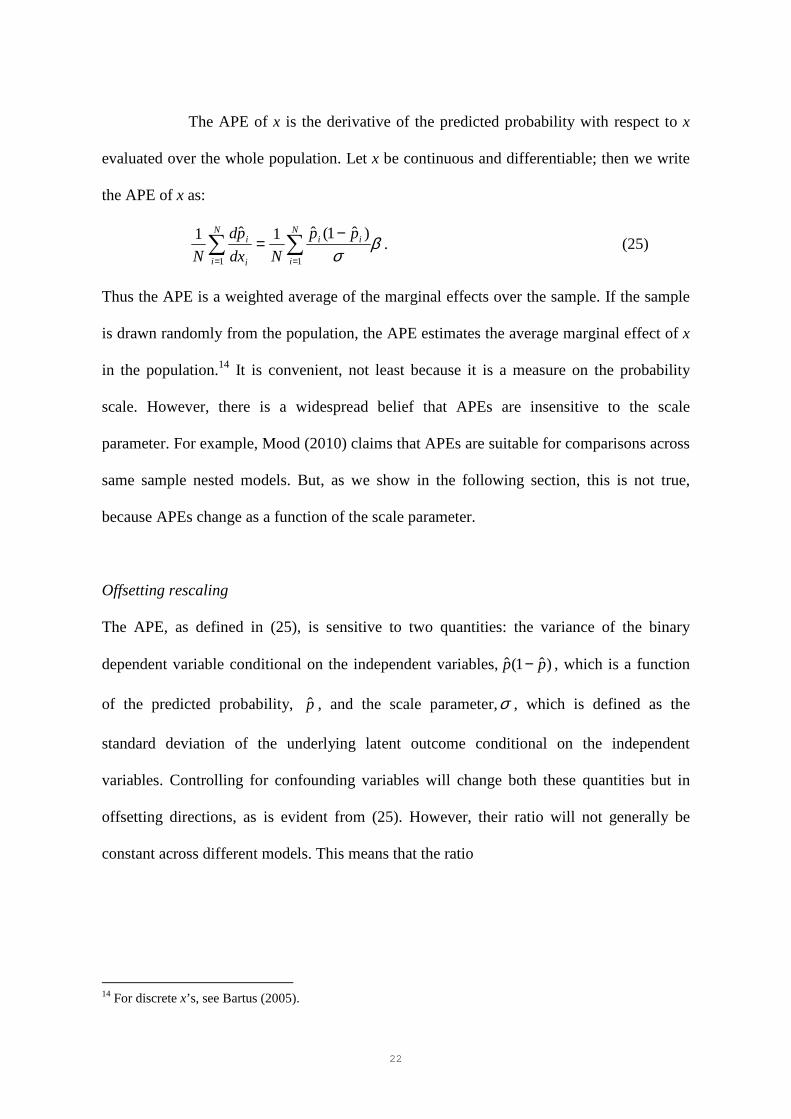
The APE of x is the derivative of the predicted probability with respect to x

evaluated over the whole population. Let x be continuous and differentiable; then we write

the APE of x as:

βσ∑ ∑

= =

−=

N

i

N

i

ii

i

i pp

Ndx

pd

N 1 1

)ˆ1(ˆ1ˆ1. (25)

Thus the APE is a weighted average of the marginal effects over the sample. If the sample

is drawn randomly from the population, the APE estimates the average marginal effect of x

in the population.14 It is convenient, not least because it is a measure on the probability

scale. However, there is a widespread belief that APEs are insensitive to the scale

parameter. For example, Mood (2010) claims that APEs are suitable for comparisons across

same sample nested models. But, as we show in the following section, this is not true,

because APEs change as a function of the scale parameter.

Offsetting rescaling

The APE, as defined in (25), is sensitive to two quantities: the variance of the binary

dependent variable conditional on the independent variables, ˆ(1 )p p− , which is a function

of the predicted probability, p , and the scale parameter,σ , which is defined as the

standard deviation of the underlying latent outcome conditional on the independent

variables. Controlling for confounding variables will change both these quantities but in

offsetting directions, as is evident from (25). However, their ratio will not generally be

constant across different models. This means that the ratio

14 For discrete x’s, see Bartus (2005).

23

∑

∑

=

=

−

−

=N

iyx

R

yxyx

N

izyx

F

zyxzyx

pp

N

pp

N

xAPE

zxAPE

1

1.

..

)ˆ1(ˆ1

)ˆ1(ˆ1

)(

)|(

βσ

βσ

(26)

Will not equal .yx z

yx

ββ unless

∑∑==

−=

− N

i R

yxyxN

i F

zyxzyx pppp

11

.. )ˆ1(ˆ)ˆ1(ˆ

σσ. (27)

The ratio F

R

σσ varies between 1 (when z is uncorrelated with y) and 0 (when x has no

direct effect), while the ratio

2

1 1 1

2

1 1 1

ˆ ˆ ˆ ˆ(1 )

ˆ ˆ ˆ ˆ(1 )

N N N

yx z yx z yx z yx zi i i

N N N

yx yx yx yxi i i

p p p p

p p p p

⋅ ⋅ ⋅ ⋅= = =

= = =

− −=

− −

∑ ∑ ∑

∑ ∑ ∑ (28)

is bounded between ∞ and 0 (for the same configurations of the relations between x, z, and

y).

Certainly there could be cases in which (27) would hold––that is, where the

change in the ratio of residual standard deviations across two models exactly equals the

change in the variance of the predicted probabilities––but there is no reason to think it will

always hold. Furthermore, although we can observe the ratio of the variances of the

predicted probabilities, we cannot observe F

R

σσ , and so the rescaling of the APE is

unknown.

24

Applying our method to APEs

Because APEs are sensitive to rescaling, we cannot directly compare the uncontrolled APE

of x with the controlled counterpart (controlling for z) to obtain an estimate of the change in

the effect of x on the underlying latent variable when we introduce confounders. However,

we can apply the method developed in this paper to APEs, so solving the problem

encountered in (26) and (27). Calculating the APE for the logit model involving zɶ , we

obtain the following

1

1

ˆ ˆ(1 )1( | )

ˆ ˆ(1 )1( | )

Nyx z yx z

yx zyx zi F

Nyx z yx z yx

yxi F

p p

APE x z Np pAPE x z

N

β βσββ

σ

⋅ ⋅⋅

⋅=

⋅ ⋅

=

−

= =−

∑

∑ ɶ ɶɶ, (29)

Which follows because of (9) and (10) and because ˆ ˆyx z yx zp p⋅ ⋅= ɶ . While (29) casts the

change in APEs in ratios as in (5b), we can easily derive the change in differences between

APEs:

( )1

ˆ ˆ(1 )1( | ) ( | )

Nyx z yx z

yx yx zi F

p pAPE x z APE x z

Nβ β

σ⋅ ⋅

⋅=

−− = −∑ɶ . (30)

Note that (38) is not equal to the difference we would normally calculate,

namely )|()( zxAPExAPE − .

To summarize, APEs cannot generally be used for decomposing effects as in

linear models because one cannot compare the uncontrolled APE with its controlled

counterpart. However, applying the method developed in this paper to APEs produces the

same result as applying the method to logit coefficients (i.e., captures “pure” confounding,

net of any rescaling). For example, the ratio in (29) equals the ratio in (12b). The reason for

this is that our method holds constant both the rescaling of the logit coefficients and the

rescaling of APEs. Applying our method to APEs yields a measure of the extent to which

25

the effect of x on y is mediated or confounded by z on the probability scale, which may be a

more interpretable effect measure than logit coefficients.

Examples

To illustrate the method of decomposing the change in logit coefficients into confounding

and rescaling, we now turn to two examples. The first is a simulation study that illustrates

how naïve comparisons of probit coefficients may fail. The second example is based on

data from the National Education Longitudinal Study of 1988 (NELS88).15 We decompose

the effect of parental income on the probability of graduating from high school, and we

expect that the effect of parental income will decline when student achievements and

parental educational attainments are controlled. We also report the results in APEs.

Simulation study: Failing to detect change in probit coefficients across models

We draw N = 2,000 independent observations. Let x be a continuous normally distributed

random variable, and let e and v be two Normally distributed random error terms. We

construct a confounder, z, such that

6.5z x v= + ,

which gives a 0.135 correlation between x and z. We construct the underlying outcome, y*,

such that

* 2 2 8y x z e= + + .

The observed binary dependent variable y is a dichotomization of y* around the median of

the distribution (ensuring 50 percent in each category of y). We report the estimates from

15 We use approximately 8,000 8th grade students in 1988 who were re-interviewed in 1990, 1992, 1994, and 2000. We have relevant background information and information on the educational careers of the students. For a full description of the variables used in this example, see Curtin et al (2002). We do not comment further on attrition, because we present the example as an illustration of how rescaling operates.

26

three probit16 models with y as dependent variable in Table 2. The first model includes x,

the second model includes both x and z, and the third includes x and the x-residualized z, zɶ .

A straightforward comparison of the coefficients of x in models 1 and 2 would

lead to the conclusion that z does not mediate, confound, or explain the effect of x on y.

However, because x and z are correlated and because z has an independent effect on y, we

know that z is a true confounder. Using the method proposed here reveals this. Comparing

the coefficients of x in models 3 and 4 shows a marked reduction: 0.475-0.254 = 0.221 or

46.5 percent using formula (12c). Moreover, because this example involves a single z, we

may exploit the property that the Z-value for the coefficient of z in model 2 equals the ZC-

value for the difference in the coefficients of x between models 3 and 2 (see (19)). Its value

is 0.244/0.010 ≈ 24.9, which is much larger than the critical value of 1.96. We therefore

conclude that the effect of x is truly confounded by z and that the reduction of the effect of x

is highly statistically significant. This example illustrates how naïve comparisons may mask

true confounding in cases where confounding and rescaling exactly offset each other.

Because our method decomposes the coefficient change into confounding and rescaling, we

are able to detect whether the x-y relationship is truly confounded by z.

-- TABLE 2 HERE --

Example based on NELS88

In this example we study how the effect of parental income on high school graduation

changes when we control for student academic ability and parental educational attainment.

We use NELS88 and our final sample consists of 8,167 students. The dependent variable is

16 We use probit models, because we use logit models in the next example. However, using either probit or logit models returns near-identical results.

27

a dichotomy indicating whether the student completed high school (= 1) or not (= 0). The

explanatory variable of interest is a measure of yearly family income. Although the variable

is measured on an ordered scale with 15 categories, for simplicity we use it here as a

continuous variable. We include three control variables: these are student academic ability

and the educational attainment of the mother and of the father.17 We derive the ability

measure from test scores in four different subjects using the scoring from a principal

component analysis.18 We standardize both the family income variable and the three control

variables to have mean zero and variance of unity. We estimate five logistic models and

report the results in Table 3.

In M1 we find a positive logit coefficient of 0.935 for the effect of family

income on high school completion. Controlling for student academic ability in M2 reduces

the effect to 0.754. A naïve comparison would thus suggest that academic ability mediates

100*(0.935-0.754)/0.935 = 19.4 percent of the effect of family income on high school

graduation. However, such a comparison conflates confounding and rescaling. To remedy

this deficiency, we use the estimate of family income in M3, where we have included the

residualized student academic ability measure. The estimate is 1.010 and is directly

comparable with the estimate in M2. Using our method we obtain a 100*(1.010-

0.754)/1.010 = 25.3 percent reduction due to confounding, net of rescaling. Because we

only include a single control variable (academic ability), we know that the test statistic for

academic ability in M2 equals the test statistic for the difference in the effect of family

income in M3 and M2. Because we have good reasons to expect that academic ability

17 Parental education is coded in seven, ordered discrete categories. To keep the example simple, we include father’s and mother’s education as continuous covariates, although a dummy-specification would have given a more precise picture of the relationship with the dependent variable. 18 These tests are in reading, mathematics, science, and history. The variables are provided in the public use version of NELS88. The eigenvalue decomposition revealed one factor accounting for 78.1 percent of the total variation in the four items.

28

reduces the effect of family income on high school completion, we use a one-sided

hypothesis and thus a critical value of 1.64. We obtain ZC = 0.672/0.042 ≈ 15.84, and we

therefore conclude that academic ability mediates the effect of family income on high

school completion.

-- TABLE 3 HERE --

In Table 3 we also report estimates from two further logistic models. M4 adds father’s and

mother’s educational attainment and M5 includes the family income residualized

counterparts of all three control variables. A naïve researcher would compare the effect of

family income in M1 (0.935) and M4 (0.386), and report a reduction of 58.7 percent.

However, using our method we would compare the effect of family income in M5 (2.188)

and M4 (0.386). This suggests a substantially larger reduction of 82.4 percent. Using the

formula in (18) we obtain a ZC of 18.88 and thereby conclude that the reduction is

statistically significant. Moreover, our method also provides us with an estimate of how

much rescaling masks the change caused by confounding. Using the decomposition

expressed in ratios in (14a):

Naïve Confounding Rescaling

0.386 2.188 0.386

0.935 0.935 2.188

2.420 5.668 0.427.

yx yx z yx

yx z yx z yx z

b b b

b b b⋅

⋅ ⋅ ⋅

= ×

⇓

= ×

= ×

ɶ

ɶ

��� ��� ���

⇕

While confounding reduces the effect by a factor of 5.7, rescaling counteracts this reduction

with an increase of about 0.427-1 = 2.3 times. In this case rescaling plays an important role

29

in masking the true change due to confounding. Not surprisingly, rescaling has a

statistically significant effect: using (20) returns a ZS of 14.24, which is far larger than the

critical value of 1.64.

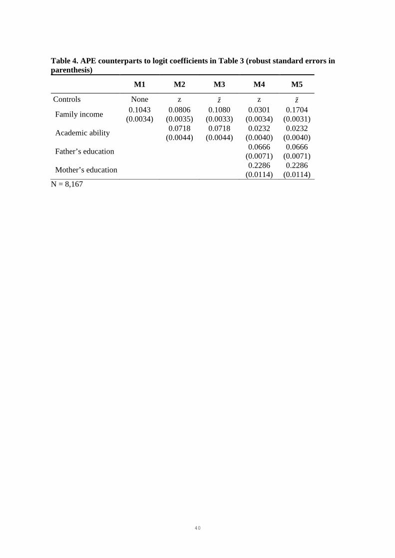
In the final part of this example we reproduce Table 4, but we replace the

logit estimates with APEs.19 In M1 we observe that a standard deviation increase in family

income increases the probability of completing high school by 10.4 percent. Controlling for

student academic ability in M2 changes the effect to 8.1 percent, a reduction of 22.7

percent. However, using the specification in M3 returns a slightly different result, namely a

25.4 percent reduction. Using more decimals than the ones presented in Table 4, this

percentage reduction exactly equals the reduction calculated with the logit coefficients in

Table 3. In light of equation (29), this finding is what we would have expected. Moreover,

as noted in a previous section, APEs somewhat offset rescaling. The naïve comparison

using logit coefficients returned a 19.4 percent reduction, while the naïve counterpart for

APEs returned a 22.7 percent reduction. The naïve comparison based on APEs is thus

closer to the true reduction (25.3 percent).

Turning to models M4 and M5 in Table 4, naïvely comparing the effect of

family income in M1 and M4 returns a 71.1 percent reduction, while correctly comparing

the effect in M5 and M4 returns an 82.3 percent reduction. With sufficient decimals the

latter reduction exactly equals the one based on the logit coefficients in Table 2. Moreover,

comparing the family income APE in M1 and M5 clearly shows that APEs can be highly

sensitive to rescaling. Conditional on M1 holding true, we would estimate that a standard

deviation increase in family income would increase the probability of completing high

school by around 10 percent. However, conditional on M4 (and thus M5) holding true (the

19 We use the user-written margeff command in Stata to calculate the APEs (Bartus 2005).

30

model which, in this example, we would take as the full model), the effect is around 17

percent. Although the results point in the same direction, there is a substantial difference

between the effect sizes.

Similar to the decomposition of the naïve ratio of logit coefficients into

confounding and rescaling, we can report an APE counterpart:

Naïve Confounding APE "rescaling"

( ) ( | ) ( )

( | ) ( | ) ( | )

0.1043 0.1704 0.1043

0.0301 0.0301 0.1704

3.465 5.661 0.612.

APE x APE x z APE x

APE x z APE x z APE x z= ×

⇓

= ×

= ×

ɶ

ɶ

����� ����� �����

⇕

From the decomposition we see that the ratio measuring confounding equals the one found

with logit coefficients. However, the rescaling is smaller for APEs (0.612 – that is, closer to

unity) than for logit coefficients (0.427).

-- TABLE 4 HERE --

Conclusion

Winship and Mare (1984) noted that logit coefficients are not directly comparable across

same sample nested models, because the logit fixes the error variance at an arbitrary

constant. While the consequences of this identification restriction for the binary logistic

model are well-known in the econometric literature, no-one has as yet solved the problem

that emerges when comparing logit coefficients across nested models. This has led many

applied quantitative sociologists to believe that confounding works the same way for the

binary logit or probit regression model as for the linear regression model. In this paper we

31

remedy the previous lack of attention to the undesirable consequences of rescaling for the

interpretation of sequentially controlled logit coefficients by developing a method that

allows us to identify the separate effects of rescaling and confounding.

Our exposition and its illustration through the simulated example and the

analysis of NELS data lead us to five main points. First, naïve comparisons of logit

coefficients across same sample nested models should be avoided. Such comparisons may

mask or underestimate the true change due to confounding. Second, using our method

resolves the problem, because it decomposes the naïve coefficient change into a part

attributable to confounding (of interest to researchers) and into a part attributable to

rescaling (of minor interest for researchers). Third, our method provides easily calculated

test statistics that enable significance tests of both confounding and rescaling. Fourth, APEs

can be highly sensitive to rescaling but, fifthly, applying our method to APEs overcomes

this problem.

Rescaling will always increase the apparent magnitude of the coefficient of a

variable20 and this commonly counteracts the effect of the inclusion of confounding

variables, which are most often expected to reduce the effect of the variable of interest.

This creates a serious problem for applied research. Observing a relatively stable coefficient

of interest across models which successively introduce blocks of control variables typically

leads researchers to the conclusion that the effect is “persistent” and robust to the addition

of control variables (see our simulation example). Furthermore, even if researchers find that

the controlled effect is smaller than the uncontrolled effect, the difference may nevertheless

be underestimated because of rescaling. The same goes for average partial effects, which up

until now have been claimed to be insensitive to rescaling. In any of these cases

20 This happens when both y* and x, y* and z, and x and z are all positively correlated, e.g., when y* is passing an educational threshold, x is some parental background characteristic, and z is cognitive ability.

32

conclusions about the impact of confounding cannot be justified unless we use the method

proposed in this paper. And, as we noted at the outset, the problem we address here is not

confined to binary logit or probit models: it applies to all non-linear models for categorical

or limited dependent variables (such as the complementary log-log) and it occurs in all

applications that use logit or probit models (such as discrete time event history models) and

their extensions (such as multilevel logit models and multinomial logits).

33

Appendix: Proof of equation (19)

In this appendix we prove equation (19). We show that testing 0yx z yx zb b⋅ ⋅− =ɶ amounts to

testing 0yz xb ⋅ = , because it holds that:

yx z yx z yz x zxb b b θ⋅ ⋅ ⋅− =ɶ , (A1)

where zxθ is a linear regression coefficient relating x to z: zxz x lθ= + , where l is a random

error term. (A1) says that the part of the xy-relationship confounded by z may be expressed

as the product of the logit coefficient relating z to y net of x, and the linear regression

coefficient relating x to z. Whenever 0yz xb ⋅ = , (A1) equals zero and thus, since yz xb ⋅ is

measured on the same scale as the difference yx z yx zb b⋅ ⋅−ɶ , testing 0yz xb ⋅ = amounts to

testing whether the difference yx z yx zb b⋅ ⋅−ɶ is zero.

However, the equality in (A1) must hold in order for the test to be effective.

We therefore prove that the equality in (A1) holds. Exploiting the derivations for linear

models by Clogg, Petkova, and Haritou (1995) and the method developed in this paper, we

have that

.

*( )

yz x

yxz yz xz yx

yx z yx z zyx z yx z

F F

sr r r r

sb b

β

β βσ σ

⋅ ⋅⋅ ⋅

−−

− = =ɶ

ɶ

����

,

where ijr denotes the correlation between variables i and j, and sk denotes the standard

deviation of variable k. From simple definitions we find that:

( )

( )* ** *

yz xxz

b

y yxy x y x xz xz xz yz xz yx

yz x xz x z zyz x xz yx z yx z

F F F

s ssr r r r r r r r

b s s sb b b

θ

θθ

σ σ σ

⋅

⋅⋅ ⋅ ⋅

− −= = = = −ɶ

������

.

34

We have thus proved the equality in (A1) and shown that, in the three-variable case, (19) is

a test of the significance of confounding net of rescaling. In Karlson, Holm, and Breen

(2010) we exploit the property in (A1) to develop a new method for decomposing total

effects into direct and indirect effects for logit and probit models.

35

References

Agresti, Alan. 2002. Categorical Data Analysis. Second Edition. New Jersey: Wiley &

Sons.

Allison, Paul D. 1999. “Comparing Logit and Probit Coefficients Across Groups.”

Sociological Methods & Research 28:186-208.

Amemiya, Takeshi. 1975. “Qualitative Response Models.” Annals of Economic and Social

Measurement 4:363-388.

Bartus, Thamás. 2005. “Estimation of marginal effects using margeff.” Stata Journal

5:309-329.

Blalock, Hubert M. 1979. Social Statistics, 2nd ed. rev. New York: McGraw-Hill.

Clogg, Clifford C., Eva Petkova, and Adamantios Haritou. 1995. “Statistical Methods for

Comparing Regression Coefficients Between Models.” The American Journal of Sociology

100:1261-1293.

Cramer, J.S. 2003. Logit Models. From Economics and Other Fields. Cambridge:

Cambridge University Press.

Curtin, Thomas R., Steven J. Ingels, Shiying Wu, and Ruth Heuer. 2002. User’s Manual.

National Education Longitudinal Study of 1988: Base-Year to Fourth Follow-up Data File

36

User’s Manual (NCES 2002-323). Washington, DC: U.S. Department of Education,

National Center for Education Statistics.

Hoetker, Glenn. 2004. “Confounded coefficients: Accurately comparing logit and probit

coefficients across groups.” Working Paper.

––––– . 2007. “The use of logit and probit models in strategic management research:

Critical issues.” Strategic Management Journal 28:331-343.

Karlson, Kristian Bernt, Anders Holm, and Richard Breen. 2010. “Total, Direct, and

Indirect Effects in Logit Models.” Working Paper.

Kendall, Patricia and Paul L. Lazarsfeld. 1950. “Problems of Survey Analysis.” Pp. 133-

196 in Continuities in Social Research, edited by Merton, Robert K. and Paul L. Lazarsfeld.

Glencoe, Illinois: The Free Press.

Lazarsfeld, Paul F. 1955. “The Interpretation of Statistical Relations as a Research

Operation.” Pp. 115-125 in The Language of Social Research, edited by Paul F. Lazarsfeld

and Morris Rosenberg. Glencoe, Illinois: The Free Press.

Lazarsfeld, Paul F. 1958. “Evidence and Inference in Social Research.” Daedalus 87:99-

130.

37

Long, J. S. 1997: Regression Models for Categorical and Limited Dependent Variables.

Thousand Oaks: Sage.

Long, J.S. and Jeremy Freese. 2005. Regression Models for Categorical Dependent

Variables Using Stata, 2nd ed. College Station: Stata Press.

Maddala, G. S. 1983. Limited-Dependent Variables and Qualitative Variables in

Economics. New York: Cambridge University Press.

McKelvey, Richard D. and William Zavoina. 1975. “A Statistical Model for the Analysis of

Ordinal Level Dependent Variables.” Journal of Mathematical Sociology 4:103-120.

Mood, Carina. 2010. “Logistic Regression: Why We Cannot Do What We Think We Can

Do, and What We Can Do About It.” European Sociological Review 26:67-82.

Powers, Daniel A. and Yu Xie. 2000. Statistical Methods for Categorical Data Analysis.

San Diego: Academic Press.

Simon, Herbert A. 1954. “Spurious Correlation: a Causal Interpretation.” Journal of the

American Statistical Association 49:467-479.

Yatchew, Adonis and Zvi Griliches. 1985. “Specification Error in Probit Models.” The

Review of Economics and Statistics 67:134-139.

38

White, Halbert. 1982. “Maximum likelihood estimation of misspecified models.”

Econometrica 50:1–25.

Williams, Richard. 2009. “Using Heterogeneous Choice Models to Compare Logit and

Probit Coefficients Across Groups.” Sociological Methods & Research 37:531-559.

Winship, Christopher and Robert D. Mare. 1984. “Regression Models with Ordinal

Variables.” American Sociological Review 49:512-525.

Wooldridge, Jeffrey M. 2002. Econometric Analysis of Cross Section and Panel Data.

Cambridge, MA: MIT Press.

39

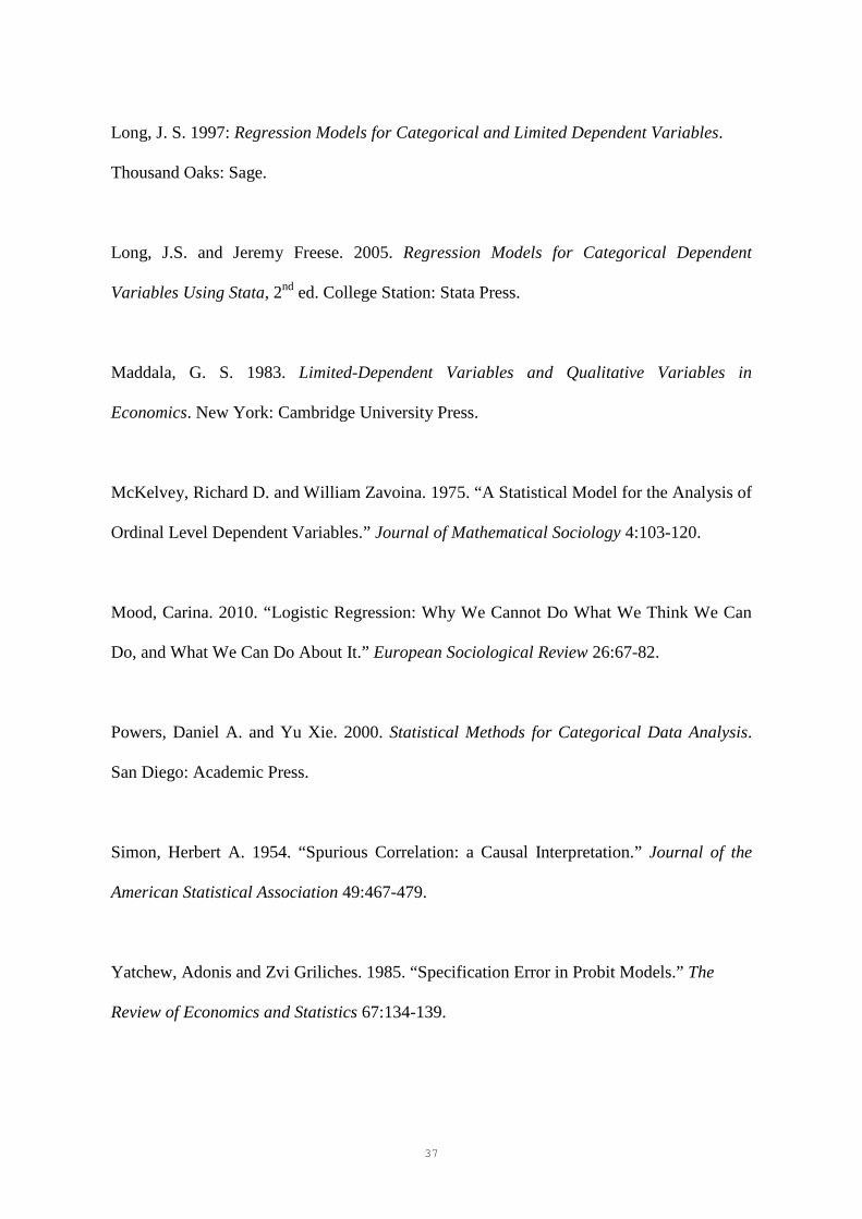
Table 1. Normal and y-standardized logit coefficients from the two models Model 1 Model 2

yxb sdYyxb yx zb ⋅ sdY

yx zb ⋅

x 0.360 0.195 0.466 0.166 z - - 0.947 0.336

*ˆ( )SD y 1.849 2.815

Pseudo-R2 0.022 0.188 Table 2. The effect of x on y from simulated data. Probit coefficients. Model 1 Model 2

(z) Model 3

( zɶ )

Coef. SE Coef. SE Coef. SE x 0.252 0.029 0.254 0.039 0.475 0.041 zor zɶ - - 0.244 0.010 0.244 0.010 Intercept 0.002 0.028 0.020 0.037 0.001 0.037 Pseudo-R2 0.028 0.478 0.478

Table 3. Controlling the effect of family income on high school graduation. Logit-coefficients (robust standard errors in parenthesis)

M1 M2 M3 M4 M5

Controls None z zɶ z zɶ

Family income 0.935

(0.032) 0.754

(0.034) 1.010

(0.033) 0.386

(0.042) 2.188

(0.093)

Academic ability

0.672 (0.042)

0.672 (0.042)

0.298 (0.050)

0.298 (0.050)

Father’s education

0.856 (0.092)

0.856 (0.092)

Mother’s education

2.936 (0.217)

2.936 (0.217)

Intercept 1.981

(0.035) 2.132

(0.040) 2.132

(0.040) 4.298

(0.188) 4.298

(0.188) Pseudo-R2 0.138 0.180 0.180 0.421 0.421

LogL -3021.5 -2872.8 -2872.8 -2028.6 -2028.6

N = 8,167

40

Table 4. APE counterparts to logit coefficients in Table 3 (robust standard errors in parenthesis)

M1 M2 M3 M4 M5

Controls None z zɶ z zɶ

Family income 0.1043

(0.0034) 0.0806

(0.0035) 0.1080

(0.0033) 0.0301

(0.0034) 0.1704

(0.0031)

Academic ability

0.0718 (0.0044)

0.0718 (0.0044)

0.0232 (0.0040)

0.0232 (0.0040)

Father’s education

0.0666 (0.0071)

0.0666 (0.0071)

Mother’s education

0.2286 (0.0114)

0.2286 (0.0114)

N = 8,167

41

Kristian Bernt Karlson is a PhD student at the Danish School of Education, Aarhus

University. He works in the areas of social stratification and mobility research with

particular interest in the modeling of discrete choice processes.

Anders Holm is professor in quantitative methods at The Danish School of Education,

Aarhus University. He holds a PhD in economics and works in the areas of sociology of

education, industrial relations, and micro econometrics. He has previously published in

Social Science Research, Sociological Methods and Research, and Research in Social

Stratification and Mobility.

Richard Breen is professor of Sociology and Co-Director of the Center for the Study of

Inequality and the Life Course at Yale University. Recent papers have appeared in

American Journal of Sociology, European Sociological Review, and Sociological Methods

and Research.