Comparing coefficients of nested nonlinear probability

Comparing coefficients of nested nonlinearprobability models using khb

Ulrich Kohler

Joined Work with Kristian B. Karlson and Anders Holm

9th German Stata Users Group MeetingBamberg

01 July 2011

U. Kohler (WZB) Comparing Coeficients with khb 01 July 2011 1 / 25

Outline

1 Introduction

2 The KHB-method

3 The command khb

4 Application

5 References


Introduction

Outline

1 Introduction

2 The KHB-method

3 The command khb

4 Application

5 References


Introduction

Reasons to compare

Depvar (Y)Keyvar (X)bX |Z

Mediator (Z)


Introduction

Reasons to compare

Depvar (Y)Keyvar (X)bX


Introduction

Reasons to compare


bX |Z

Mediator (Z)

bX − bX |Z


Introduction

Reasons to compare

Depvar (Y)

Keyvar (X)

bX

bX |Z

Control (Z)

bX − bX |Z


Introduction

Reasons to compare


bX |Z

Control (Z)

bX − bX |Z


Introduction

The problem

We are interested in obtaining βR − βF from the following models forlatent Y ∗:

Y ∗ = αF + βF X + γF Z + δF C + ε (1)Y ∗ = αR + βRX + δRC + ε (2)

Having ovserved Y with value 0 if Y ∗ < τ and 1 if Y ∗ ≥ τ we canobtain the logit/probit estimates with

bF =βF

σFand bR =

βR

σR(3)

Note: We identify the underlying coefficients of interest relative to ascale unknown to us.


The KHB-method

Outline

1 Introduction

2 The KHB-method

3 The command khb

4 Application

5 References


The KHB-method

General idea

The KHB-method extracts from Z the information that is not containedin X . This is done by calculating the residuals of a linear regression ofZ on X , i.e,

R = Z − (a + bX ) , (4)

where a and b are the estimated regression parameters of a linearregression.

Instead of using equation (2) we then use

Y ∗ = α̃R + β̃RX + γ̃RR + δ̃RC + ε . (5)


The KHB-method

Difference of coefficients

As R and Z differ only in the component in Z that is correlated with X ,model (1) is no more predictive than model (5), and consequently theresiduals have the same standard deviation so that

σ̃R = σF (6)

As β̃R = βR we can write

b̃R − bF =β̃R

σ̃R− βF

σF=βR − βF

σF. (7)

Hence, the difference obtained reflects the difference searched dividedby some common scale.


The KHB-method

Derived statistics

Confounding ratiob̃R

bF=

βRσFβFσF

=βR

βF, (8)

Counfounding percentage

100 · b̃R − bF

b̃R= 100 ·

βRσF− βF

σFβRσF

= 100 · βR − βF

βR, (9)


The KHB-method

Significance test for the difference in effects

Analyitcally derived standard errors for the difference in effectsexist.Based on the delta method (Sobel, 1982).Simple for one X and ond Z but fairly complicated for situationswith more than one X , Z .Karlson et al. (2010) has more details; also see our Stata Journalpublications (in Press)


The command khb

Outline

1 Introduction

2 The KHB-method

3 The command khb

4 Application

5 References


The command khb

Syntax

khb model-type depvar key-vars ‖ mediator-vars[

if][

in][, options

]model-type can be any of regress, logit, ologit, probit,oprobit, cloglog, slogit, scobit, rologit, clogit, andmlogit.

key-vars may contain factor variables

aweights, fweights, iweights, and pweights are allowed if theyare allowed for the specified model type.


The command khb

Options (most important ones)

options descriptionconcomitant(varlist) concomitantsdisentangle disentangle difference of effectssummary summary of decompositionvce(vcetype) robust or cluster clustvarape decomposition using avg. partial effectsverbose show restricted and full modelkeep keep residuals of mediators


Application

Outline

1 Introduction

2 The KHB-method

3 The command khb

4 Application

5 References


Application

Preliminaries

Examples from educational sociologySubset of Danish National Longitudinal Survey (DLSY).Reproduce analysis presented by Karlson and Holm (2011).

. use dlsy_khb, clear

. describe

Contains data from dlsy_khb.dtaobs: 1,896vars: 8 17 Jan 2011 10:26size: 49,296 (99.9% of memory free)

storage display valuevariable name type format label variable label

edu byte %20.0g edu Educational attainmentupsec byte %10.0g yesno Complete upper secondary

education (Gymnasium)univ byte %13.0g yesno Complete University educationfgroup byte %9.0g fgroup Father´s social group/classfses float %9.0g Father´s SES, standardized with

mean 0 and sd 1abil double %10.0g Standardized ability measure,

with mean 0 and sd 1intact byte %9.0g yesno Intact familyboy byte %9.0g yesno Boy

Sorted by:


Application

Basic use

. khb logit univ fses || abil, c(intact boy)

Decomposition using the KHB-Method

Model-Type: logit Number of obs = 1896Variables of Interest: fses Pseudo R2 = 0.19Z-variable(s): abilConcomitant: intact boy

univ Coef. Std. Err. z P>|z| [95% Conf. Interval]

fsesReduced .5459815 .0779806 7.00 0.000 .3931424 .6988206

Full .3817324 .0778061 4.91 0.000 .2292353 .5342295Diff .1642491 .0293249 5.60 0.000 .1067734 .2217247


Application

Confounding ratio/percentage

. khb logit univ fses || abil, c(intact boy) summary notable



Summary of confounding

Variable Conf_ratio Conf_Pct Resc_Fact

fses 1.4302727 30.08 1.0602422


Application

Option ape

. khb logit univ fses || abil, c(intact boy) ape summary

Decomposition using the APE-Method



fsesReduced .0384906 .0054429 7.07 0.000 .0278226 .0491585

Full .0269113 .0054476 4.94 0.000 .0162343 .0375884Diff .0115792 .0020667 5.60 0.000 .0075286 .0156298

Note: Standard errors of difference not known for APE method


Variable Conf_ratio Conf_Pct Dist_Sens

fses 1.4302727 30.08 .95931864


Application

Disentangle contributions of mediators

. khb logit univ fses || abil intact boy, s d not


Model-Type: logit Number of obs = 1896Variables of Interest: fses Pseudo R2 = 0.19Z-variable(s): abil intact boy



fses 1.5207722 34.24 1.1317064

Components of Difference

Z-Variable Coef Std_Err P_Diff P_Reduced

fsesabil .1661177 .0301003 83.56 28.61

intact .020142 .0144611 10.13 3.47boy .0125359 .011524 6.31 2.16


Application

More than one key variable

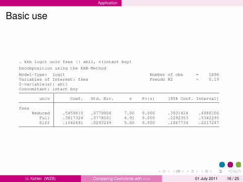
. khb logit univ boy intact || abil, c(fses) s


Model-Type: logit Number of obs = 1896Variables of Interest: boy intact Pseudo R2 = 0.19Z-variable(s): abilConcomitant: fses


boyReduced 1.06178 .1848087 5.75 0.000 .6995613 1.423998

Full .9821406 .1848351 5.31 0.000 .6198704 1.344411Diff .0796391 .133004 0.60 0.549 -.1810438 .3403221

intactReduced 1.129767 .7386976 1.53 0.126 -.3180536 2.577588

Full 1.08391 .7386558 1.47 0.142 -.3638292 2.531648Diff .0458575 .1328438 0.35 0.730 -.2145116 .3062266



boy 1.0810873 7.50 1.0033213intact 1.0423075 4.06 1.03542


Application

Categorical variables

. xtile catabil = abil, n(4)

. tab catabil, gen(catabil)

. khb logit univ i.fgroup || catabil2-catabil4, c(intact boy) s d


Application

Ordered outcome

. forv i = 1/3 {2. quietly eststo: khb ologit edu fses || abil, out(`i´) ape s3. }

. esttab, scalars("ratio_fses Conf.-Ratio" "pct_fses Conf.-Perc.")

(1) (2) (3)edu edu edu

fsesReduced -0.103*** 0.0643*** 0.0385***

(-11.33) (10.72) (9.27)

Full -0.0755*** 0.0472*** 0.0283***(-8.02) (7.76) (7.23)

Diff -0.0272*** 0.0170*** 0.0102***(-6.50) (6.44) (5.95)

N 1896 1896 1896Conf.-Ratio 1.360 1.360 1.360Conf.-Perc. 26.48 26.48 26.48

t statistics in parentheses* p<0.05, ** p<0.01, *** p<0.001


Application

Multinomial outcome

. forv i = 2/3 {2. quietly eststo: khb mlogit edu fses || abil, out(`i´) base(1) s3. }

. esttab, scalars("ratio_fses Conf.-Ratio" "pct_fses Conf.-Perc.")

(1) (2)edu edu

fsesReduced 0.423*** 0.779***

(7.63) (9.30)

Full 0.313*** 0.552***(5.70) (6.68)

Diff 0.109*** 0.227***(5.93) (6.04)

N 1896 1896Conf.-Ratio 1.349 1.411Conf.-Perc. 25.88 29.15

t statistics in parentheses* p<0.05, ** p<0.01, *** p<0.001


References

Outline

1 Introduction

2 The KHB-method

3 The command khb

4 Application

5 References


References

References

Karlson, K. B. and A. Holm. 2011. Decomposing primary andsecondary effects: A new decomposition method. Research inStratification and Social Mobility 29: XXXX.

Karlson, K. B., A. Holm, and R. Breen. 2010. Comparing regressioncoefficients between models using logit and probit: a new method.Unpublished paper (currently under review).

Sobel, M. E. 1982. Asymptotic confidence intervals for indirect effectsin structural equation models. In Sociological Methodology 1982, ed.L. S., 290–312. Washington D.C.: American SociologicalAssociation.


Documents

Comparing coefficients of nested nonlinear probability