Outline

1 Significance testingAn example with two quantitative predictorsANOVA f-testsWald t-testsConsequences of correlated predictors

2 Model selectionSequential significance testing

Nested modelsAdditional Sum-of-Squares principleSequential testing

the adjusted R2

Likelihoodthe Akaike criterion

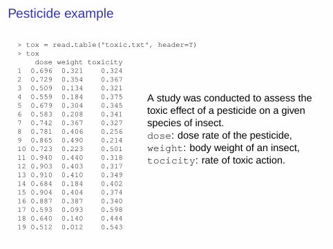
Pesticide example

> tox = read.table("toxic.txt", header=T)> tox

dose weight toxicity1 0.696 0.321 0.3242 0.729 0.354 0.3673 0.509 0.134 0.3214 0.559 0.184 0.3755 0.679 0.304 0.3456 0.583 0.208 0.3417 0.742 0.367 0.3278 0.781 0.406 0.2569 0.865 0.490 0.21410 0.723 0.223 0.50111 0.940 0.440 0.31812 0.903 0.403 0.31713 0.910 0.410 0.34914 0.684 0.184 0.40215 0.904 0.404 0.37416 0.887 0.387 0.34017 0.593 0.093 0.59818 0.640 0.140 0.44419 0.512 0.012 0.543

A study was conducted to assess thetoxic effect of a pesticide on a givenspecies of insect.dose : dose rate of the pesticide,weight : body weight of an insect,tocicity : rate of toxic action.

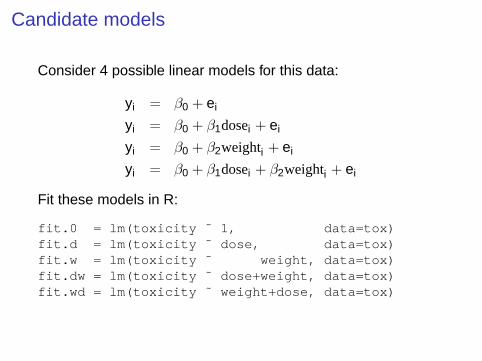
Candidate models

Consider 4 possible linear models for this data:

yi = β0 + ei

yi = β0 + β1dosei + ei

yi = β0 + β2weighti + ei

yi = β0 + β1dosei + β2weighti + ei

Fit these models in R:

fit.0 = lm(toxicity ˜ 1, data=tox)fit.d = lm(toxicity ˜ dose, data=tox)fit.w = lm(toxicity ˜ weight, data=tox)fit.dw = lm(toxicity ˜ dose+weight, data=tox)fit.wd = lm(toxicity ˜ weight+dose, data=tox)

Comparing models using anova

> anova(fit.0, fit.d)Analysis of Variance TableModel 1: toxicity ˜ 1Model 2: toxicity ˜ dose

Res.Df RSS Df Sum of Sq F Pr(>F)1 18 0.15762 17 0.1204 1 0.0372 5.26 0.035 *

> anova(fit.w, fit.wd)Analysis of Variance TableModel 1: toxicity ˜ weightModel 2: toxicity ˜ weight + dose

Res.Df RSS Df Sum of Sq F Pr(>F)1 17 0.0654992 16 0.034738 1 0.030761 14.168 0.001697 **

Testing β1 = 0 (dose effect) gives a different result whetherweight is included in the model or not.

Comparing models using anova

We did two different tests:

H0 : [β1 = 0|β0] is testing β1 = 0 (or not) given that only theintercept β0 is in the model

H0 : [β1 = 0|β0, β2] is testing β1 = 0 assuming that anintercept β0 and a weight effect β2 are in the model.

They make different assumptions, may reach different results.

The anova function, when given two (or more) differentmodels, does an f-test by default.Source df SS MSβ2|β0 1 SS(β2|β0) SS(β2|β0)/1β1|β0, β2 1 SS(β1|β0, β2) SS(β1|β0, β2)/1Error n − 3

∑ni=1(yi − yi)

2 SSError/(n − 3)Total n − 1

∑ni=1(yi − y)2

Fact: if H0 is correct, F = MS(β1|β0, β2)/MSError∼ F1,n−3.

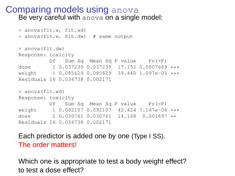
Comparing models using anovaBe very careful with anova on a single model:

> anova(fit.w, fit.wd)> anova(fit.w, fit.dw) # same output

> anova(fit.dw)Response: toxicity

Df Sum Sq Mean Sq F value Pr(>F)dose 1 0.037239 0.037239 17.152 0.0007669 ***weight 1 0.085629 0.085629 39.440 1.097e-05 ***Residuals 16 0.034738 0.002171

> anova(fit.wd)Response: toxicity

Df Sum Sq Mean Sq F value Pr(>F)weight 1 0.092107 0.092107 42.424 7.147e-06 ***dose 1 0.030761 0.030761 14.168 0.001697 **Residuals 16 0.034738 0.002171

Each predictor is added one by one (Type I SS).The order matters!

Which one is appropriate to test a body weight effect?to test a dose effect?

Comparing models using drop1

> drop1(fit.dw, test="F")Single term deletionsModel: toxicity ˜ dose + weight

Df Sum of Sq RSS AIC F value Pr(F)<none> 0.034738 -113.783dose 1 0.030761 0.065499 -103.733 14.168 0.001697 **weight 1 0.085629 0.120367 -92.171 39.440 1.097e-05 ***

> drop1(fit.wd, test="F")Single term deletionsModel: toxicity ˜ weight + dose

Df Sum of Sq RSS AIC F value Pr(F)<none> 0.034738 -113.783weight 1 0.085629 0.120367 -92.171 39.440 1.097e-05 ***dose 1 0.030761 0.065499 -103.733 14.168 0.001697 **

F-tests, to test each predictors after accounting for all others(Type III SS). The order does not matter.

Comparing models using anovaUse anova to compare multiple models.Models are nested when one model is a particular case ofthe other model.anova can perform f-tests to compare 2 or more nestedmodels

> anova(fit.0, fit.d, fit.dw)Model 1: toxicity ˜ 1Model 2: toxicity ˜ doseModel 3: toxicity ˜ dose + weight

Res.Df RSS Df Sum of Sq F Pr(>F)1 18 0.1576062 17 0.120367 1 0.037239 17.152 0.0007669 ***3 16 0.034738 1 0.085629 39.440 1.097e-05 ***

> anova(fit.0, fit.w, fit.wd)Model 1: toxicity ˜ 1Model 2: toxicity ˜ weightModel 3: toxicity ˜ weight + dose

Res.Df RSS Df Sum of Sq F Pr(>F)1 18 0.1576062 17 0.065499 1 0.092107 42.424 7.147e-06 ***3 16 0.034738 1 0.030761 14.168 0.001697 **

Parameter inference using summaryThe summary function performs Wald t-tests.

> summary(fit.d)...Coefficients:

Estimate Std. Error t value Pr(>|t|)(Intercept) 0.6049 0.1036 5.836 1.98e-05 ***dose -0.3206 0.1398 -2.293 0.0348 *

Residual standard error: 0.08415 on 17 degrees of freedomMultiple R-squared: 0.2363, Adjusted R-squared: 0.1914F-statistic: 5.259 on 1 and 17 DF, p-value: 0.03485

> summary(fit.wd)...Coefficients:

Estimate Std. Error t value Pr(>|t|)(Intercept) 0.22281 0.08364 2.664 0.01698 *weight -1.13321 0.18044 -6.280 1.10e-05 ***dose 0.65139 0.17305 3.764 0.00170 **

Residual standard error: 0.0466 on 16 degrees of freedomMultiple R-squared: 0.7796, Adjusted R-squared: 0.752F-statistic: 28.3 on 2 and 16 DF, p-value: 5.57e-06

Parameter inference using summary

The order does not matter for t-tests:

> summary(fit.wd)...Coefficients:

Estimate Std. Error t value Pr(>|t|)(Intercept) 0.22281 0.08364 2.664 0.01698 *weight -1.13321 0.18044 -6.280 1.10e-05 ***dose 0.65139 0.17305 3.764 0.00170 **...

> summary(fit.dw)...Coefficients:

Estimate Std. Error t value Pr(>|t|)(Intercept) 0.22281 0.08364 2.664 0.01698 *dose 0.65139 0.17305 3.764 0.00170 **weight -1.13321 0.18044 -6.280 1.10e-05 ***

Residual standard error: 0.0466 on 16 degrees of freedomMultiple R-squared: 0.7796, Adjusted R-squared: 0.752F-statistic: 28.3 on 2 and 16 DF, p-value: 5.57e-06

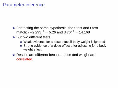
Parameter inference

For testing the same hypothesis, the f-test and t-testmatch: (−2.293)2 = 5.26 and 3.7642 = 14.168But two different tests:

Weak evidence for a dose effect if body weight is ignoredStrong evidence of a dose effect after adjusting for a bodyweight effect.

Results are different because dose and weight arecorrelated.

Consequences of correlated predictorsAlso called multicollinearity.

F-tests are order dependentCounter-intuitive results:

> summary(fit.d)... Estimate Std. Error t value Pr(>|t|)dose -0.3206 0.1398 -2.293 0.0348 *

Negative effect of dose, if dose alone!! As dose rate increases,the rate of toxic action decreases!? When results are againstintuition, this is a warning.

Correlation between dose and body weight:

> plot(dose ˜ weight, data=tox)> with(tox, cor(dose,weight))[1] 0.8943634> plot(toxicity ˜ dose, data=tox, pch=16)> plot(toxicity ˜ dose, data=tox, pch=16, col=grey(weight))> plot(toxicity ˜ dose, data=tox, pch=16, col=grey(weight * 2))

Can we have uncorrelated predictors?

Predictors x1 and x2 are uncorrelated if

n∑i=1

(xi1 − x1)(xi2 − x2) = 0

In designed experiments we can choose combination of xi1

and xi2 values so that these predictors are uncorrelated inthe experiment.

Qualitative predictors: can also be correlated

Example: sex and smoke, in the fev data set

Completely balanced designs (more later)

Outline

1 Significance testingAn example with two quantitative predictorsANOVA f-testsWald t-testsConsequences of correlated predictors

2 Model selectionSequential significance testing

Nested modelsAdditional Sum-of-Squares principleSequential testing

the adjusted R2

Likelihoodthe Akaike criterion

Model selection

Testing parameters is the same as selecting between 2 models.In our example, we have 4 models to choose from.

1 yi = β0 + ei

2 yi = β0 + β2weighti + ei

3 yi = β0 + β1dosei + ei

4 yi = β0 + β1dosei + β2weighti + ei

H0 : [β2 = 0|β0] is a test to choose betweenmodel 1 (H0) and model 2 (Ha).

H0 : [β2 = 0|β0, β1] is a test to choose betweenmodel 3 (H0) and model 4 (Ha).

H0 : [β1 = β2 = 0|β0] is an overall test to choose betweenmodel 0 (H0) and model 4 (Ha).

Nested models

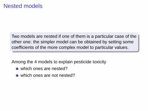
Two models are nested if one of them is a particular case of theother one: the simpler model can be obtained by setting somecoefficients of the more complex model to particular values.

Among the 4 models to explain pesticide toxicity

which ones are nested?

which ones are not nested?

Example: Cow data set

4 treatment with 4 levels of an additive in the cow feed:control (0.0), low (0.1), medium (0.2) and high (0.3)treatment : factor with 4 levelslevel : numeric variable, whose values are 0, 0.1, 0.2 or 0.3.fat : fat percentage in milk yield (%)milk : milk yield (lbs)

Are these models nested?1 fati = β0 + β2 ∗ initial.weighti + ei

2 fati = β0 + βj(i) + ei , where j(i) is the treatment # for cow i3 fati = β0 + β1 ∗ leveli + ei

Multiple R2

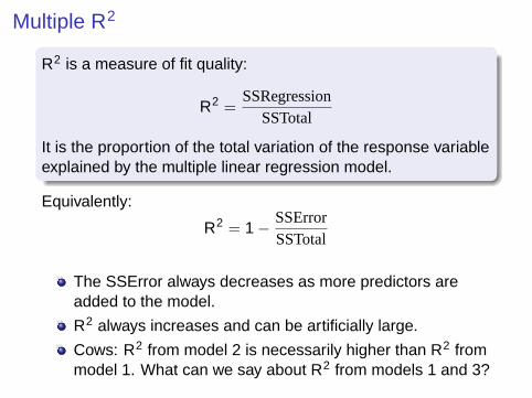
R2 is a measure of fit quality:

R2 =SSRegression

SSTotal

It is the proportion of the total variation of the response variableexplained by the multiple linear regression model.

Equivalently:

R2 = 1 − SSErrorSSTotal

The SSError always decreases as more predictors areadded to the model.

R2 always increases and can be artificially large.

Cows: R2 from model 2 is necessarily higher than R2 frommodel 1. What can we say about R2 from models 1 and 3?

Additional Sum-of-Squares principle

ANOVA F-test, to compare two nested models: a “full” anda “reduced” model.

we used it to test a single predictor.

can be used to test multiple predictors at a time.

Example:reduced: has k = 1 coefficient (other than intercept)

fati = β0 + β1 ∗ leveli + ei

full: has p =

4

coefficients other than intercept

fati = β0+β1∗leveli+β2∗initial.weighti+β3∗lactationi+β4∗agei+ei

Additional Sum-of-Squares principle

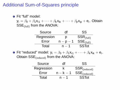
Fit “full” model:yi = β0 + β1xi1 + · · · + βkxik + · · · + βpxip + ei . ObtainSSE(full) from the ANOVA:

Source df SSRegression p SSR(full)

Error n − p − 1 SSE(full)

Total n − 1 SSTot

Fit “reduced” model: yi = β0 + β1xi1 + · · · + βkxik + ei .Obtain SSE(reduced) from the ANOVA:

Source df SSRegression k SSR(reduced)

Error n − k − 1 SSE(reduced)

Total n − 1 SSTot

Example

> full = lm(fat ˜ level+initial.weight+lactation+age, data=cow)> reduced = lm(fat ˜ level, data=cow)> anova(full)> anova(reduced)

Source df SSRegression 4 3.547

Error 45 7.952Total 49 11.499

Source df SSRegression 1 2.452

Error 48 9.047Total 49 11.499

Additional Sum-of-Squares principle

Compute the “additional sum of squares” as

SSR(full) − SSR(reduced) = SSE(reduced) − SSE(full)

which is always ≥ 0, on df = p − k = (n − p − 1) − (n − k − 1)

F-testif the reduced model is true, then

F =(SSE(reduced) − SSE(full))/(p − k)

(SSE(full))/(n − p − 1)∼ Fp−k ,n−p−1.

An f-test is used to test the reduced (H0) versus the full (Ha)model.

Hypotheses: ei ∼ normal distribution, are independent, andhave homogeneous variance.

Example

Source df SSRegression 4 3.547

Error 45 7.952Total 49 11.499

Source df SSRegression 1 2.452

Error 48 9.047Total 49 11.499

So F =

(9.047−7.952)/(48−45)7.952/45

= 2.0651 on df = 3 and 45. Thenp = 0.12.

> anova(reduced, full)Model 1: fat ˜ levelModel 2: fat ˜ level + initial.weight + lactation + age

Res.Df RSS Df Sum of Sq F Pr(>F)1 48 9.04692 45 7.9521 3 1.0948 2.0651 0.1182

Sequential testing

Often, there are many models we want to consider. Example:There are 25 = 16 models equal or nested within each of these:

fat ˜ initial.weight+lactation+age+treatmentfat ˜ initial.weight+lactation+age+level

We may not analyze them all!

Various ways to do model selection:

Many criteria: p-value from F-test, Adjusted R2, AIC, etc.

Different ways to search: backward elimination, forwardselection, stepwise selection.

Backward elimination

1 fit the full model with all the predictors2 find the predictor with the smallest f-value / t-value or

largest associated p-valueif its p-value is above some threshold, go to step 3.if not, keep the corresponding predictor and stop.

3 delete the predictor, re-fit the model and go to step 2.

Note: a threshold of p > .05 is often used, which correspondsapproximately to |t | < 2 or f < 4.

There are multiple tests being done... The Bonferroni idea israrely used, because it is overly conservative. Every term mightbe removed.

> drop1(full, test="F")fat ˜ level + initial.weight + lactation + age

Df Sum of Sq RSS AIC F value Pr(F)<none> 7.952 -81.929level 1 2.078 10.030 -72.324 11.7567 0.001308 **initial.weight 1 0.086 8.038 -83.394 0.4845 0.489987lactation 1 0.497 8.449 -80.898 2.8126 0.100463age 1 0.302 8.254 -82.065 1.7091 0.197746

> newfit = update(full, . ˜ . - initial.weight)> drop1(newfit, test="F")fat ˜ level + lactation + age

Df Sum of Sq RSS AIC F value Pr(F)<none> 8.038 -83.394level 1 2.211 10.249 -73.243 12.6541 0.000882 ***lactation 1 0.487 8.525 -82.453 2.7869 0.101829age 1 0.229 8.267 -83.990 1.3098 0.258357

> newfit = update(newfit, . ˜ . - age)> drop1(newfit, test="F")fat ˜ level + lactation

Df Sum of Sq RSS AIC F value Pr(F)<none> 8.267 -83.990level 1 2.546 10.813 -72.565 14.4756 0.0004094 ***lactation 1 0.780 9.047 -81.480 4.4365 0.0405448 *

Forward selection

1 fit the most simple model, using only predictors you want toforce in the model, not matter what. Also prepare a list ofcandidate predictors.

2 find the predictor with the largest f-value / t-value orsmallest associated p-value

if its p-value is below some threshold, go to step 3.if not, stop. Do not add the predictor to the final model.

3 Add the predictor, re-fit the model and go to step 2.

Note: a threshold of p < .05 is often used, which correspondsapproximately to |t | > 2 or f > 4.

There are multiple tests being done...

> basic = lm(fat ˜ 1, data=cow)> add1(basic, test="F",

scope = ˜initial.weight+lactation+age * level)fat ˜ 1

Df Sum of Sq RSS AIC F value Pr(F)<none> 11.499 -71.488initial.weight 1 0.566 10.933 -72.011 2.4841 0.1215677lactation 1 0.686 10.813 -72.565 3.0470 0.0872835 .age 1 0.352 11.147 -71.043 1.5163 0.2241734level 1 2.452 9.047 -81.480 13.0101 0.0007363 ***

> newfit = update(basic, . ˜ . + level)> add1(newfit, test="F",

scope = ˜initial.weight+lactation+age * level)...> newfit = update(newfit, . ˜ . + lactation)> add1(newfit, test="F",

scope = ˜initial.weight+lactation+age * level)fat ˜ level + lactation

Df Sum of Sq RSS AIC F value Pr(F)<none> 8.267 -83.990initial.weight 1 0.012 8.254 -82.065 0.0694 0.7934age 1 0.229 8.038 -83.394 1.3098 0.2584

Stepwise selection

start with some model, simple or complex

do a forward step as well as a backward step

until no predictor should be added, and no predictor shouldbe removed.

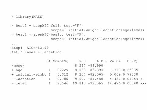
> library(MASS)

> best1 = stepAIC(full, test="F",scope=˜ initial.weight+lactation+age * level)

> best2 = stepAIC(basic, test="F",scope=˜ initial.weight+lactation+age * level)

...Step: AIC=-83.99fat ˜ level + lactation

Df SumofSq RSS AIC F Value Pr(F)<none> 8.267 -83.990+ age 1 0.229 8.038 -83.394 1.310 0.25835+ initial.weight 1 0.012 8.254 -82.065 0.069 0.79338- lactation 1 0.780 9.047 -81.480 4.437 0.04054 *- level 1 2.546 10.813 -72.565 14.476 0.00040 ***

Warnings

Forward selection, backward selection, stepwise selectioncan all miss an optimal model. Forward selection has thepotential of ’stopping short’.

They may not agree.

No adjustment for multiple testing... It is important to startwith a model that is not too large, guided by biologicalsense.

They can only compare nested models.

The adjusted R2

Recall R2 =SSRegression

SSTotal= 1 − SSError

SSTotalalways increases and

can be artificially large.

Adjusted R2

adjR2 = 1 − MSErrorSSTotal/(n − 1)

= 1 − n − 1n − 1 − k

(1 − R2)

where k is the number of coefficients (other than the intercept).It is penalized version of R2. The more complex the model, thehighest the penalty.

As k goes up, R2 increases but n − 1 − k decreases.

adjusted R2 may decrease when the added predictors donot improve the fit.

MSError and adjusted R2 are equivalent for choosingamong models.

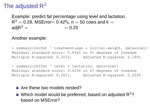
The adjusted R2

Example: predict fat percentage using level and lactation.R2 = 0.28, MSError= 0.42%, n = 50 cows and k =adjR2 = = 0.25

Another example:

> summary(lm(fat ˜ treatment * age + initial.weight, data=cow))Residual standard error: 0.4362 on 41 degrees of freedomMultiple R-squared: 0.3215, Adjusted R-squared: 0.1891

> summary(lm(fat ˜ level + lactation, data=cow))Residual standard error: 0.4194 on 47 degrees of freedomMultiple R-squared: 0.2811, Adjusted R-squared: 0.2505

Are these two models nested?

Which model would be preferred, based on adjusted R2?based on MSError?

Likelihood

The likelihood of a particular value of a parameter is theprobability of obtaining the observed data if the parameter hadthat value. It measures how well the data supports thatparticular value.

Example: tiny wasp are given the choice between two femalecabbage white butterfly. One of them recently mated (so hadeggs to be parasitized), the other not.

n = 32 wasps, y = 23 chose the mated female. Letp = proportion of wasps in the population that would make thegood choice.

Likelihood of p = 0.5, as if the wasps have no clue?

Log-likelihood

Likelihood of p = 0.5, as if the wasps have no clue:L(p = 0.5|Y = 23) = IP{Y = 23|p = 0.5} = 0.0065 fromBinomial formula:

L(p) =

(3223

)p23(1 − p)9

Most often, it is easier to work with the log of the likelihood:

log L(p|Y = 23) = log((

3223

)p23(1 − p)9

)= log

(3223

)+ 23 log(p) + 9 log(1 − p)

and log L(0.5) = log(0.0065) = −5.031

Maximum likelihood

The maximum likelihood estimate of a parameter is the value ofthe parameter for which the probability of obtaining theobserved data if the highest. It’s our best estimate.

Sometimes there are analytical formulas, which coincidewith other estimation methods.

Many times we find the maximum likelihood numerically

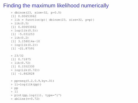
Finding the maximum likelihood numerically> dbinom(23, size=32, p=0.5)[1] 0.00653062> lik = function(p){ dbinom(23, size=32, p=p)}> lik(0.5)[1] 0.00653062> log(lik(0.5))[1] -5.031253> lik(0.2)[1] 3.158014e-10> log(lik(0.2))[1] -21.87591

> 23/32[1] 0.71875> lik(0.72)[1] 0.1552330> log(lik(0.72))[1] -1.862828

> pp=seq(0.2,0.9,by=.01)> ll=log(lik(pp))> pp> ll> plot(pp,log(ll), type="l")> abline(v=0.72)

Likelihood ratio test

Idea: if p = 0.5 is false, then the likelihood of p = 0.5 will be

much lower than the maximum likelihood, the ratioL(p)

L(0.5)will

be large, i.e. the difference in log-likelihoods will be large:log L(p) − log L(0.5).

LRT to test α = α0

Test statistic: X 2 = 2 ∗ (log L(α) − log L(α0))

Null distribution: if H0: α = α0 is true then X 2 has achi-square distribution approximately, with df=# ofparameters in α.

Here we want to test H0: p = 0.5.x2 = 2 ∗ (−1.86) − 2 ∗ (−5.03) = 6.337 on df= 1 here. We getp = 0.012: strong evidence that p 6= 0.5.

Likelihood ratio test for dose and weightLRT of H0: βdose= 0, after accounting for a weight effect:

> drop1(fit.dw, test="Chisq")Single term deletionsModel: toxicity ˜ dose + weight

Df Sum of Sq RSS AIC Pr(Chi)<none> 0.034738 -113.783dose 1 0.030761 0.065499 -103.733 0.000518 ***weight 1 0.085629 0.120367 -92.171 1.179e-06 ***

−2∗L(βdose= 0)+2∗L(βdose) = −103.733+113.783+2 = 12.05and IP

{X 2

df=1 > 12.05}

= 0.000518.

Compare with the f-test based on SS:

> drop1(fit.dw, test="F")Single term deletionsModel: toxicity ˜ dose + weight

Df Sum of Sq RSS AIC F value Pr(F)<none> 0.034738 -113.783dose 1 0.030761 0.065499 -103.733 14.168 0.001697 **weight 1 0.085629 0.120367 -92.171 39.440 1.097e-05 ***

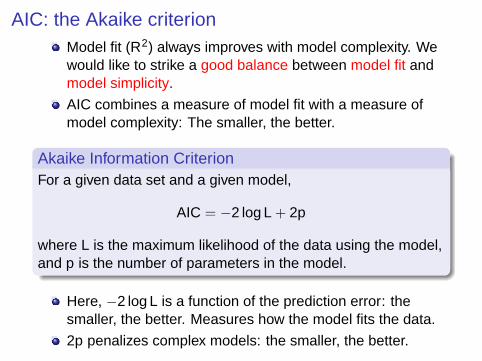
AIC: the Akaike criterionModel fit (R2) always improves with model complexity. Wewould like to strike a good balance between model fit andmodel simplicity.

AIC combines a measure of model fit with a measure ofmodel complexity: The smaller, the better.

Akaike Information CriterionFor a given data set and a given model,

AIC = −2 log L + 2p

where L is the maximum likelihood of the data using the model,and p is the number of parameters in the model.

Here, −2 log L is a function of the prediction error: thesmaller, the better. Measures how the model fits the data.

2p penalizes complex models: the smaller, the better.

AIC: the Akaike criterion

StrategyConsider a number of candidate models. They need not benested. Calculate their AIC. Choose the model(s) with thesmallest AIC.

Theoretically: AIC aims to estimate the prediction accuracyof the model for new data sets. Up to a constant.

The absolute value of AIC is meaningless. The relative AICvalues, between models, is meaningful.

Often there are too many models, we cannot get all theAIC values. We can use stepwise selection.

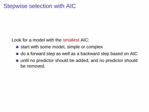
Stepwise selection with AIC

Look for a model with the smallest AIC:

start with some model, simple or complex

do a forward step as well as a backward step based on AIC

until no predictor should be added, and no predictor shouldbe removed.

> library(MASS)> stepAIC(basic,scope= ˜ initial.weight+lactation+age * level)Step: AIC=-83.99fat ˜ level + lactation

Df Sum of Sq RSS AIC<none> 8.267 -83.990+ age 1 0.229 8.038 -83.394+ initial.weight 1 0.012 8.254 -82.065- lactation 1 0.780 9.047 -81.480- level 1 2.546 10.813 -72.565

> fullt = lm(fat ˜ treatment+initial.weight+lactation+age,data=cow)

> stepAIC(fullt,scope= ˜ initial.weight+lactation+age * treatment+level)

...Step: AIC=-80.76fat ˜ treatment + lactation

Df Sum of Sq RSS AIC<none> 8.141 -80.755+ age 1 0.256 7.885 -80.353+ initial.weight 1 0.002 8.139 -78.766- lactation 1 0.686 8.827 -78.710- treatment 3 2.672 10.813 -72.565

BIC: the Bayesian information criterion

For standard models,

BIC = −2 log L + log(n) ∗ p

p is the # of parameters in the model, n is the sample size.

Theoretically: BIC aims to approximate the posteriorprobability of the model. Up to a constant.The absolute value of BIC is meaningless. The relative BICvalues, between models, is meaningful.The smaller, the better.The penalty in BIC is stronger than in AIC: AIC tends toselect more complex models, BIC tends to select simplermodels.In very simplified terms: AIC is better when the purpose isto make predictions. BIC is better when the purpose is todecide what terms truly are in the model.

BIC: the Bayesian information criterion

In R: use the option k=log(n) and plug-in the correct samplesize n. Then remember the output is really about BIC (not AIC).

> stepAIC(full, scope=˜ initial.weight+lactation+age * level,k=log(50))

...Step: AIC=-78.25fat ˜ level + lactation

Df Sum of Sq RSS AIC<none> 8.267 -78.254- lactation 1 0.780 9.047 -77.656+ age 1 0.229 8.038 -75.746+ initial.weight 1 0.012 8.254 -74.417- level 1 2.546 10.813 -68.741

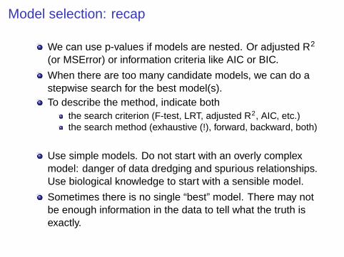
Model selection: recap

We can use p-values if models are nested. Or adjusted R2

(or MSError) or information criteria like AIC or BIC.

When there are too many candidate models, we can do astepwise search for the best model(s).To describe the method, indicate both

the search criterion (F-test, LRT, adjusted R2, AIC, etc.)the search method (exhaustive (!), forward, backward, both)

Use simple models. Do not start with an overly complexmodel: danger of data dredging and spurious relationships.Use biological knowledge to start with a sensible model.

Sometimes there is no single “best” model. There may notbe enough information in the data to tell what the truth isexactly.