Embed Size (px)
Citation preview

RANDOM REGRESSION IN ANIMAL BREEDING
Course Notes
Jaboticabal, SP Brazil November 2001
Julius van der WerfUniversity of New EnglandArmidale, Australia
1 Introduction.......................................................................................................................................22 Exploring correlation patterns in repeated measurements...................................................................63 Covariance Functions......................................................................................................................12
3-1 The use of Covariance Functions ............................................................................................123-2 Estimating covariance functions..............................................................................................143-3 Estimation of Covariance Functions with REML....................................................................22
4 Application of Covariance Functions in mixed models...................................................................254-1 Modeling covariance functions ...............................................................................................254-2 Equivalence Covariance Functions and Random Regression..................................................274-3 Estimating CF coefficients with the random regression model ...............................................31
6 Analyzing patterns of variation .......................................................................................................427 Summarizing Discussion.................................................................................................................46
Those notes are mainly based on a course given in Guelph (Canada) in 1997Chapter 5 from these notes have been omitted

2
1 Introduction
In univariate analysis the basic assumption is that a single measurement arises
from a single unit (experimental unit). In multivariate analysis, not one measurement
but a number of different characteristics are measured from each experimental design,
e.g. milk yield, body weight and feed intake of a cow. These measurements are
assumed to have a correlation structure among them. When the same physical quantity
is measured sequentially over time on each experimental unit, we call them repeated
measurements, which can be seen as a special form of a multivariate case. Repeated
measurements deserve a special statistical treatment in the sense that their covariance
pattern, which has to be taken into account, is often very structured. Repeated
measurements on the same animal are generally more correlated than two
measurements on different animals, and the correlation between repeated
measurements may decrease as the time between them increases. Modeling the
covariance structure of repeated measurements correctly is of importance for drawing
correct inference from such data.
Measurements that are taken along a trajectory can often be modeled as a
function of the parameters that define that trajectory. The most common example of a
trajectory is time, and repeated measurements are taken on a trajectory of time. The
term ‘repeated measurement’ can be taken literally in the sense that the measurements
can be thought of as being repeatedly influenced by identical effects, and it is only
random noise that causes variation between them. However, repeatedly measuring a
certain characteristic may give information about the change over time of that
characteristic. The function that describes such a change over time my be of interest
since it may help us to understand or explain, or to manipulate how the characteristic
changes over time. Common examples in animal production are growth curves and
lactation curves.
Generally, we have therefore two main arguments to take special care when
dealing with repeated measurements. The first is to achieve statistically correct models
that allow correct inferences from the data. The second argument is to obtain
information on a trait that changes gradually over time.

3
Experiments are often set up with repeated measurements to exploit these two
features. The prime advantage of longitudinal studies (i.e. with repeated
measurements over time) is its effectiveness for studying change. Notice that the
interpretation of change may be very different if it is obtained from data across
individuals (cross sectional study) or on repeated measures on the same individuals.
An example is given by Diggle et al. (1994) where the relationship between reading
ability and age is plotted. A first glance at the data suggests a negative relationship,
because older people in the data set tended to have had less education. However,
repeated observations on individuals showed a clear improvement of reading ability
over time.
The other advantage of longitudinal studies is that it often increases statistical
power. The influence of variability across experimental units is canceled if
experimental units can serve as their own control.
Both arguments are very important in animal production as well. A good
example is the estimation of a growth curve. When weight would be regressed on time
on data across animals, not only would the resulting growth curve be more inaccurate,
but also the resulting parameters might be very biased if differences between animals
and animals’ environments were not taken into account.
Models that deal with repeated measurements have been often used in animal
production. In dairy cattle, the analysis of multiple lactation records is often
considered using a ‘repeatability model’. The typical feature of such a model from the
genetic point of view is that repeated records are thought of expressions of the same
trait, that is, the genetic correlation between repeated lactation is considered to be
equal to unity. Models that include data on individual test days have often used the
same assumption. Typically, genetic evaluation models that use measures of growth
do often consider repeated measurements as genetically different (but correlated)
traits. Weaning weight and yearling weight in beef cattle are usually analyzed in a
multiple trait model.
Repeatability models are often used because of simplicity. With several
measurements per animal, they require much less computational effort and less
parameters than a multiple trait model. A multiple trait model would often seem more
correct, since they allow genetic correlations to differ between different
measurements. However, covariance matrix for measurements at very many different

4
ages would be highly overparameterised. Also, an unstructured covariance matrix may
not be the most desirable for repeated measurements that are recorded along a
trajectory. As the mean of measurements is a function of time, so also may their
covariance structure be. A model to allow the covariance between measurements to
change gradually over time, and with the change dependent upon differences between
times, can make use of a covariance function.
As was stated earlier, repeated measurements can often be used to generate
knowledge about the change of a trait over time. Whole families of models have been
especially designed to describe such changes as regression on time, e.g. lactation
curves and growth curves. The analysis may reveal causes of variation that influence
this change. Parameters that describe typical features of such change, e.g. the slope of
a growth curve, are regressions that may be influenced by feeding levels, environment,
or breeds. There may also be additive genetic variation within breeds for such
parameters. One option is then to estimate curve parameters for each animal and
determine components of variation for such parameters. Another option is use a model
for analysis that allows regression coefficients to vary from animal to animal. Such
regression coefficients are then not fixed, but are allowed to vary according to a
distribution that can be assigned to them, therefore indicated as random regression
coefficients.
This course will present models that use random regression in animal
breeding. Typical applications are for traits that are measured repeatedly along a
trajectory, e.g. time. Different random regression models will be presented and
compared. The features of random regression models and estimation of their
parameters will be discussed. Alternative approaches to deal with repeatedly measured
traits along a trajectory are the use of covariance functions, and use of multiple trait
models. These approaches have much in common, since they all deal with
changing covariances along a trajectory. Differences that seem to exist are most often
due to the differences in the model, and generally not necessarily due to the approach
followed. This course will present and discuss the different methods, and show where
they can be equivalent. Different models that allow the study of genetic aspects of
changes of traits along a trajectory will be presented and discussed.
Most of the examples will refer to test day production records in dairy cattle,
since test day models have been used mostly to develop and compare random

5
regression models. However, the procedures and models presented have a much wider
scope for use, since many characters have multiple expressions, and often there is an
interest in how the expression changes over time. A good example is the analysis of
traits related to growth. Another generalization is that the methodology developed not
necessarily refers to traits that are modeled as a function of time (i.e. regressed on a
time variable). In these notes, other extensions will be presented as well, e.g.
expressions of traits being function of production level.

6
2 Exploring correlation patterns in repeated measurements
There are several ways to explore the correlation structure in repeated measurements
Diggle et al. (1994) . Graphical displays can be very useful to identify patterns
relevant to certain questions, e.g. the relationship between response and explanatory
variables. Figures 2-1, 2-2, and 2-3 (adapted from Diggle et al. 1994) illustrate this by
showing graphs for body weight in 5 pigs as a function of time. Figure 2-1 shows the
lines connecting the weights on an individual pig in consecutive weeks. This graph
shows that (1) pigs gain weight over time, 2) pigs that are largest at the beginning tend
to be largest at the end, and 3) the variation among weights is lower at the beginning
than at the end.
The second observation is important in relation to correlation structure, and
has important biological implications. Figure 2-2 gives a clearer picture of the second
point. By plotting deviations from the mean, the graph is magnified. In Figure 2-2, we
observe that lines do cross quite often, and rankings do change for different times on
the axis. Measurements tend to cross less in the later part of the experiment, i.e.
correlations might be higher in later part of the trajectory. With many individuals, it is
more difficult to interpret such graphs.
0
10
20
30
40
50
60
70
80
1 2 3 4 5 6 7 8 9
weeks
wei
gh
t
Figure 2.1. Body weight for 5 pigs measured at 9 consecutive weeks

7
-8
-6
-4
-2
0
2
4
6
8
1 2 3 4 5 6 7 8 9
weeks
res
idu
al
we
igh
t
Figure 2-2. Residual body weight (deviation from week mean) for 5 pigs measured at
9 consecutive weeks
Exact values such as correlations between measurements at different time points can
not be obtained from graphs like in Figure 2-1. When observations are made at equally
spaced times, associations between repeated measurements at two fixed times are
easily plotted and measured in terms of correlations. With unequally spaced
observations, this is less evident. Diggle et al. (1994) suggest to use a variogram. This
is a function that describes the association among repeated values and is easily
estimated with irregular observation times. A variogram is defined as
γ ( ) [{ ( ( ) ( )} ],u E y t y t u u= − − ≥12
2 0
where γ ( )u describes the squared differences between measurements that are u time
units apart. The variogram is calculated from observed half-squared differences
between pairs of residuals,
v r rijk ij ik= −12
2( )
and the corresponding time differences

8
u t tijk ij ik= −
where yij is the jth observation on animal i, and residuals are r y E yij ij ij= − ( ) , i.e.
they can be calculated as deviations from contemporary means. If the times are
regular, !( )γ u is estimated as the average of all vijk corresponding to the particular u.
With irregular sampling times, the variogram can be estimated from the data pairs
(uijk,vijk) by fitting a curve A variogram for the example of Figure 2-2 is given in
Figure 2-3. As an example, the point for u=8 is obtained as the average of the half-
squared differences between the residual for the first and the 9th observation on the
five pigs: !( ) {( ) ( )} /. .γ u y y y yi ii
= = − − −=∑8 51
2 1 1 9 91
52 ,
where y j. is the average of the jth observation.
0
2
4
6
8
10
12
14
16
18
1 2 3 4 5 6 7 8
u
gam
a(u
)
Figure 2-3. Variogram for the pig example, showing γ ( )u (gama(u)) for u=1,…8 (u=
distance between measurements in weeks)
A structure often used in repeated measurements to describe the correlation matrix is
the autocorrelation structure. We can define autocorrelation as the correlation between
two measurements as a function of the distance (in time) between the measurements.
The autocorrelation function can be estimated from the variogram as
!( ) !( ) / !ρ γ σu u= −1 2 , where !σ 2 is the ‘process variance’, which is calculated as the
average of all half squared differences 12
2( )y yij lk− with i ≠ l.
9
There exist several types of correlation models. In a uniform correlation
model, we assume that there is a positive correlation ρ between any two
measurements on the same individual (independent of time). In matrix terms the
correlation matrix between observation on the same animal is written as
V I J0 1= − +( )ρ ρ
where I is the identity matrix and J is a matrix with all elements equal to 1. The
uniform correlation model is used in what is generally called a ‘repeatability model’ in
animal breeding.
In the exponential correlation model , correlations between two observations
at the same animal at times j and k are
v t tjk j k= − −σ φ2 exp( | |) .
In this model, the correlation between a pair of measurements on the same individual
decreases towards zero as the time separation between measurements increases. The
rate of decay is faster for larger values of φ. If the observation times are equally
spaced, than the correlation between the jth and the kth measurements can be
expressed asv jk
j k= −σ ρ2 | | , where ρ φ= −e . Sometimes the correlation decreases
slow initially, and then decreases sharply towards zero. Such behaviour may be better
described by a Gaussian correlation function:
v t tjk j k= − −σ φ2 2exp( ( ) ) .
The exponential correlation model is sometimes called the first order
autoregressive model. In such a model, the random part of an observation depends
only on the random part of the previous observation: ε ρεj j jz= +−1 , where z j is an
independent random variable. Models where random variables (e.g. errors) depend on
previous observations are called ante-dependence models, and a when random
variable depend on p previous variables we have a pth order Markov model.
In general we can distinguish three different sources of random variation that
play a role in repeated measurements (Diggle et al., 1994):
• Random effects. When the units on which we have repeated measurements are
sampled at random from a population, we can observe variation between units.
Some units are on average higher responders than other units. In animal breeding,

10
an obvious example of such effects are animal effects, or more specific, the
(additive) genetic effects of animals.
• Serial correlation. This refers to part of the measurement that is part of a time
varying stochastic effect. Such an effect causes correlation between observations
within a short time interval, but common effects are less correlated if
measurements are further away.
• Measurement error. This is an error component of an observation which effect is
each time independent of any other observations.
If a model is build that accommodates these three random effects, the variance
structure of each of the effects needs to be described. Diggle et al (1990) give a
general formula for the variance of observations on one experimental unit as
var( )ε σ τ= + +v J H I2 2 2 [2.1]
where v 2 2,σ andτ 2 are variance components for the three random effects, J is a
matrix with ones, and H is specified by a correlation function.
This model given in [2.1] often used in analysis of longitudinal data. In fact,
model [2.1] is not at all general. The random effects are assumed to be constant over
all measurements within a unit. If we think of this effect as a the genetic effect of an
animal we can imagine very well these to vary between ages (over time), and this may
even bear our special interest. Therefore, J should be replaced by a correlation
function. The serial correlation effect may be seen as the temporary environmental
effects often used in animal breeding data. For both the random and the serial
correlation effect, the question is how the correlation (c.q. covariance-) function
should be defined.
The patterns as described in this section, and as often use in the statistical
literature, show smooth functions that seem natural for many stochastic processes.
However, the additive genetic effect on a trait over time maybe more irregular. For
example, some genes could be mainly active during the first 4 months of growth of a
pig, with high correlations between measurements within this period, but other genes
may take over during the last month. Also the permanent environmental effect does

11
not necessarily follow the pattern of the correlation structures shown in this section.
In dairy cattle, the permanent environmental effect might be explained by differences
between raising of animals before first calving, possibly having a large effect on the
first part of lactation, and only then gradually decreasing. We could therefore require a
method used to describe the change of covariances over time to be flexible, and not
relying on predefined structures.
A flexible approach is to define a function for the covariance structure that is
based on regression. The next section will describe the development of covariance
functions based on regression on orthogonal polynomials. Like polynomial regression
is suitable and flexible for fitting linear function of the means, it can be used to fit
covariance structures. Alternatively, models to fit covariance structures over time
could be based on time variables defined based upon a biological model (e.g. growth
and lactation curves). Such models will be presented in a later section, when random
regression will we discussed.

12
3 Covariance Functions
3-1 The use of Covariance Functions
An individual’s phenotype changes with age. Traits that change with age can
be represented as a trajectory, that is, as a function of time. Because each character
takes on a value at each of an infinite number of ages, and its value of each age can be
considered as a distinct trait, such trajectories are referred to as ‘infinite-dimensional ‘
characters (Kirkpatrick et al., 1994).
When a phenotypical expression is repeatedly measured over a certain time
frame, we can model those a repeated measurements of genetically the same trait (rg
between measurements =1), but often it is more accurate to consider these as
expressions of genetically different, but correlated characters. Correlations can be both
through genetic and environmental causes.
Multiple measurements on a given time frame can therefore be considered as
multiple traits. However, when measurements can be randomly scattered over the time
frame, a multiple trait approach would theoretically involve an infinite number of
traits, or practically very many traits and many animals would have missing data for
most of the traits (unless they are continuously measured). A simplification is then to
limit the number of traits by defining the expression in certain periods of time as
separate traits (e.g. years or months). Such an approach has disadvantages. The first is
that we fit the covariance structure as discontinuous whereas it really is continuous.
Two measurements close to each other but in different months would have lower
correlation than two other measurements, further apart but measured in the same
month.
The second disadvantage is that it would be more tedious to account correctly
for having more measurements in the same time period. For example, milk production
in dairy is most often measured once in each lactation month. Some animals may have
two records per month by chance, and some herds may have more frequent sampling
schemes, e.g. automated daily recording. Accounting for repeated measurements per
time period requires an additional variable for the permanent environmental effects.

13
The third disadvantage of a multiple trait model for traits at many different
ages is that the correlation matrix is not structured. For measurements taken along a
trajectory, the covariance structure should take account of a certain ordering of the
measurements in time. In other words, the correlation between measurements should
somehow be related to the time that lies between the measurements.
Rather than applying models with a finite number of traits, an infinite-
dimensional approach can be followed. In a infinite-dimensional approach, the
covariance structure is modeled as a covariance function, being a function of the
covariance between times ti and tj, where the times should be points along a defined
trajectory. A covariance function allows
! a gradual change of covariances over time
! a relationship between the covariance and time differences
! predicting variances and covariances for points along the trajectory, even though
no, or few observations have been made for these points, but using information
from all other measurements
The advantages of using a covariance function are analogous to the advantage of using
regression. The purpose of estimating a regression model y= xβ+ e, is to predict y-
values for given x-values. For x-values that had never observations attached to them,
we can still predict y-values. This may seem obvious when we model observations on
animals (i.e. fitting means). However, the same principles apply when we fit
variances. Yet, it is common in animal breeding that we use for the best prediction of
a trait at a certain time ti only the value of a variance close to ti, rather than making
use of information on variance at all points measured. A covariance function would
use such information by regressing covariance on time. Furthermore, it predicts
covariances between traits at the full trajectory, rather than at some points that we
have measurements on.
The interest in traits that change over time is often in parameters that describe
that change, and particularly, in animal breeding, genetic parameters. Such parameters
might give information on whether and how we can manipulate such changes, i.e.
how we manipulate growth or lactation curves. Covariance functions provide a
method for analyzing independent components of variation that reveal specific

14
patterns of change of the character over time. For example, components of variance
might be mostly associated with traits values in particular parts of the trajectory, e.g.
milk in later lactation, or growth early in life. Techniques for finding such components
will be presented in this chapter 6.
In summary, covariance functions can be used for traits that 1) (gradually)
change over time, 2) are measured on trajectories, and 3) can be called 'infinite
dimensional'. Examples are: growth, lactation, survival. Covariance functions are
applied because it allows 1) accurate modeling of the variance-covariance structure
of the traits described, 2) it is able to predict covariance structures at any point along a
continuous (time) scale 3) it gives more flexibility in using measurements taken on
any moment along the trajectory without having to correct them to certain landmark
ages, 4) it provides a methodology to analyse patterns of covariance that are associated
with particular changes of the trait along the trajectory.
3-2 Estimating covariance functions
A covariance function can be defined as “ a continuous function to give the variance
and covariance of traits measured at different points on a trajectory”. Covariance
function can be used to describe the phenotypic covariance structure, but in principle
it is appropriate to define a covariance function for each of the random effects that
explain variation. In an animal breeding context, it may be most common to use a
covariance function to describe the genetic covariance structure, and we will use that
mostly in the examples.
Covariance functions can be defined based on many regression models. We
will choose Kirkpatrick et al (1990) by using a regression on Legendre polynomials.
This method provide a smooth fit to orthogonal functions of the data. In mathematical
terms, a covariance function (CF), e.g. for the covariance between breeding values ul
and um on an animal for traits measured at ages xl and xm is:
cov(ul,um)= (ƒ(xl,xm)= i
k
j
k
=
−
=
−
∑ ∑0
1
0
1
φi(xl)φj(xm)kij [3-1]
where φi is the ith (i=0,..,k-1) polynomial for a k-order of fit, x is a standardized age
15
(-1 ≤ x ≤ 1) and kij are the coefficients of the CF. The ages can be standardized by
defining amin and amax as the first and the latest time point on the trajectory considered,
and standardizing age ai to xi= [2( ai-amin) /( amax-amin)]-1.
The CF can be written in matrix notation as
!G = ΦΦΦΦKΦΦΦΦ'
where !G is the genetic covariance matrix of order t for breeding values at t given
ages, ΦΦΦΦ is a t by k matrix with orthogonal polynomials The matrix ΦΦΦΦ can also be
written as MΛΛΛΛ, with M being a t by k matrix with elements mij= ai(j-1) (i=1,..t; j=1,..k),
and ΛΛΛΛ being a matrix of order k with polynomial coefficients.
We follow here (partly) the example given by Kirkpatrick et al., 1990.
Consider having a genetic covariance matrix for weight measurements of mice at 2,3,
and 4 weeks of age. The standardized age vector is: a= [-1, 0 1]. A covariance
functions can be estimated based on a variance covariance matrix of observations on a
number of age points. For example, and additive genetic covariance matrix that was
previously estimated:
~. .
. .
. .
G =436 522 3 424 2
522 3 808 664 7
424 2 664 7 558
The jth normalized Legendre polynomial is given by the formula
φj j
m
m
jj mx
j j
m
j m
jx( ) ( )
/
= + −
−
=
−∑1
2
2 1
21
2 2
0
22
The matrix with CF coefficients can be estimated with the first three polynomials (a 3-
order fit). The matrix ΛΛΛΛ for the first 3 Legendre polynomials is a 3 by 3 matrix:
Λ =−0 7071 0 0 7906
0 122 0
0 0 2 3717
. .
.
.

16
The matrix M has t rows (t=3), one for each age measured, and k columns (k=3), for
the mean, linear and quadratic fit, respectively:
M =−1 1 1
1 0 0
1 1 1
The resulting matrix ΦΦΦΦ is constructed as MΛΛΛΛ, i.e. ΦΦΦΦ is:
Φ =−
−0 7071 12247 15811
0 7071 0 0 7906
0 7071 12247 15811
. . .
. .
. . .
and the coefficient matrix K is estimated as !~K G t= − −Φ Φ1 , where the -t superscript
refers to the inverse of the transpose. The estimated coefficient matrix becomes:
!. .
. . .
. . .
K =−−
− −
1348 665 1117
665 24 3 14 0
1117 14 0 14 5
the coefficient of the covariance function are obtained in C K= Λ Λ' :
!. . .
. . .
. . .
C =−−
− −
808 0 712 214 5
7120 36 4 40 7
214 5 40 7 816
and in terms of equation [3-1], the covariance function is
ƒ(x1,xm)=
808+ 71.2(x1+xm) +36.4xl xm -40.7(x1 2xm + x1xm 2) - 214.5(x1
2+xm2) +81.6( x1
2xm2).

17
Using this function we can estimate the covariance between the age combinations
represented in !G , but by interpolation we can also estimate covariance between ages that
were never measured. For example, the covariance between weight at 3 (x1=0) and 3.5
(x2=0.5) weeks of age is ƒ(0, 0.5) = 808+ 71.2*(0.5) - 214.5*(0.52) =789.9.
Notice that in this example we had a full fit of ~G . In that case, the matrix ΦΦΦΦ has an
inverse, and estimation of the coefficient matrix K is straightforward. Also, the matrix ~G
is fully obtained by ΦΦΦΦ !K ΦΦΦΦ', i.e. we basically have drawn a regression line through all
the observed points. However, we are most often interested in a reduced fit where k < t.
This is especially important for larger t.
In a reduced fit, we try to estimate the coefficients for K so that the fit is optimal.
For this purpose, we can use least squares techniques. We can consider the model
~G = ΦΦΦΦKΦΦΦΦ' +ϑ [3-2]
where ~G is the observed genetic covariance matrix for the ages defined in ΦΦΦΦ, and ϑ
is a matrix with sampling errors, i.e. differences between the covariances predicted by
the covariance function and the observed covariances. The purpose is to estimate K
such that these differences are minimal. We can write [3-2] as a linear model by
stacking the observed covariances in the matrix ~G into a vector ~g . We obtain the
equations:
~g Xk e= + [3-3]
where X is the coefficient matrix and k is the solution vector with the elements of K
stacked into a vector. Hence, ~g ’=[ ~
( , ),...~
( , ),~
( , ),...~
( , ),...~
( , )G G t G G n G t t11 1 1 2 2 ]
The residuals e are stacked columns from the matrix ϑϑϑϑ. The coefficient matrix is
constructed from the elements in ΦΦΦΦ by taking its direct product: X= ΦΦΦΦ⊗ΦΦΦΦ. The vectors
~g and k have length t2 and k2, respectively, and the matrix X has dimensions t2 by k2.
For a 2-order fit we have:

18
Φ =−
0 7071 12247
0 7071 0
0 7071 12247
. .
.
. .
and X =
− −−− −
−
− −
05 087 087 15
05 0 087 0
05 0 87 087 15
05 087 0 0
05 0 0 0
05 0 87 0 0
05 087 087 15
05 0 087 0
05 0 87 087 15
. . . .
. .
. . . .
. .
.
. .
. . . .
. .
. . . .
Notice that since ~G is a symmetric matrix, the equations in [3-3] have a redundancy in
that there are many double elements. The equations in [4] can therefore be rewritten
by redefining ~g and k to vectors of length t(t+1)/2 and k(k+1)/2, containing only the
lower half of the matrix elements of ~G and K, respectively. The rows in X
corresponding to ~G (i,j), for i<j need to be deleted. Furthermore, the columns
corresponding to K(i,j), for i<j need to be added to the columns corresponding to
K(j,i), and the columns for K(i,j) needs to be deleted. Following these steps, the matrix
X has dimensions t(t+1)/2 and k(k+1)/2:
X =
−−
−
05 1732 15
05 0 866 0
05 0 15
05 0 0
05 0 866 0
05 1732 15
. . .
. .
. .
.
. .
. . .
The coefficients are then estimated by least squares as
! ( ' ) ' ~k X X X g= −1 [3-4]
and the matrix with CF coefficients !K is then created by unstacking !k .
Least squares estimation is appropriate if the error variance structure of the
observations is is a multiple of the identity matrix, in this case: V= var( ~g ) = var(e) = Iσ2.
However, for an estimated variance-covariance matrix this is usually not the case. The

19
elements in V contain sampling variances for the estimated (co)variance components in
~G . The sampling variance depends on the mean of the estimated variance component,
and might be very different for variances than for covariances. The diagonal elements of
V, should therefore not be expected to be the same for all the estimated variances and
covariances. Furthermore, off diagonal elements of V contain sampling covariances which
are generally not zero. A more accurate estimation of the CF coefficients would be
obtained if we apply a Generalized Least Squares procedure, i.e.
! ( ' ) ' ~k X V X X V g= − − −1 1 1 [3-5]
For a GLS estimate, sampling variances and covariances of the estimated variance
components in ~G are needed. When those components are estimated with REML,
approximate sampling (co)variances can be given, the approximation being better when
there is more data. Kirkpatrick et al (1990) presented a method to estimate elements of V
based on the particular design that is used to estimate the genetic variance components.
They distinguish half- and full sib designs and parent-offspring designs. In animal
breeding, we use often field data and an animal model to estimate covariance matrices.
Depending on the data structure, an animal model could amalgamate information from all
these designs. When approximate sampling variances are not available, a rough estimate
could be based on assuming a design that is closest to the data. For example, REML
estimates from data on dairy cattle are generally close to half sib designs, and we could
approximate the number of half sib families (s), and the number of individuals per family
(n). An approximation of the sampling covariance between ~G (i,j) and
~G (k,l) from a half
sib design is
! [ ( ! , ! ) ( ! , ! )], , , , ,Vn
Cov M M Cov M Mij kl a ij a kl e ij e kl= +16
2 [3-6]
where !Ma and !Me are the estimated mean cross products among sires and residuals,
respectively, and those crossproducts can be derived from the estimated of phenotypic and
genetic covariances, in ~P and
~G , respectively as

20
! ~ ~,M P Ge ij ij ij= − 1
4 and~ ~ ~
,Mn
G Pa ij ij ij=−
+1
4[3-7]
The covariance between cross products is,
Cov M M M M M M fij kl ik jl il jk( , ) ( ) /= + [3-8]
f is the number of degrees of freedom for the mean cross product. We can estimate this
covariance unbiasedly by replacing the M’s by their estimates from [3-7] and dividing in
[3-8] by f +2 rather than by f .
When attempting to fit a lower order of fit for a covariance function, we need test statistics
to be able to determine whether the order fitted is sufficient. Kirkpatrick et al. (1990)
suggest to use the weighted residual sums of squares:
wSSE= (~ !)' ! (~ !)g Xk V g Xk− −−1 [3-9]
as a test statistic for the goodness of fit for a particular model. The test statistic in [3-9] has
a χm p−2 - distribution, where m = t(t+1)/2 and p = k(k+1)/2, i.e. (m-p) is the degrees of
freedom for the residual sums of squares. Since the weighted sums of squares in [10]
depend on the the values estimated in !V , inferences on the model depend the the accuracy
of these estimates. For example, if values in !V are underestimated (i.e. it is assumed that
the covariances in ~G are more accurate than they actually are), the test statistic defined in
[3-9] will be overestimated, and it ill be more difficult to find a particular order of fit
sufficient. An alternative statistic for fitting covariance functions could be and F-test. The
significance of adding additional parameters to the model with k increased to k+1 (H1-
model) over a simpler model (H0 model) is tested with an Fp,dfe-test using the test
statistic
[(wSSEH0-wSSEH1)/p]/[wSSEH1/dfe] [3-10]
where dfe is equal to the degrees of freedom for the residual sums of squares for the
H0 model, and p = [(k+1)(k+2)/2]-[(k+1)k/2] = k+1.

21
Kirkpatrick et al (1990) found for the example as described in this section, and using [3-9]
that only a full order of fit would be sufficient. For k=1, they found for the test statistic
according to [10] a value of 57.3, and for k=2 they found 38.7, which are both very
significant for χ52 and χ3
2 .
However, an F-test as in [3-10] for a model with k=2 over k=1 is F23= 1.44, which is not
significant. An F-test is more sensitive to low degrees of freedom, and the Kirkpatrick
example may therefore be not ideal to compare these test statistics. The F-test is not able to
test a particular model versus the model with full fit, since wSSEH1= 0.
Table 1 shows testing of different orders of fit for a genetic covariance matrix
between six 50-day periods of first lactation records in Holsteins (Van der Werf et al.,
1997). The F-test shows that a 3-order fit was sufficient to fit the data. The wSSE
values were not significant for any of the models, although for lower orders of fit were
consistently higher than the expected value, which was df. In this example, the wSSE
values might have been underestimated because of too high value assumed for the
sampling covariances.
TABLE 3-1 Testing different orders of fit (k) for the additive genetic covariancematrix1 using covariance functions with Legendre polynomials.
k wSSE σe2 df F
1 24.66 1.23 20 - 2 18.69 1.04 18 2.87*
3 12.80 0.85 15 2.30*
4 9.93 0.90 11 0.795 7.84 1.31 6 0.32
1 The covariance matrix was of order six with covariances between six 50-day periods of milk production in firs parity Holsteins.
Like in regression analysis, we can test the Goodness of Fit of different
combinations of polynomials. For example, we can also test the fit of the first and the 3rd
order polynomial. For the Kirkpatrick example this gave a wSSE of 36.7, which is a better
fit than the first two polynomials. Notice therefore that the analysis just described are
mainly testing whether a particular polynomial explains additional variation in the fit
of ~G . It does not tell us how many regression coefficients are needed to fit the covariance

22
function. A linear combination of more polynomials could be sufficient to explain a large
part of the variance in ~G . We can evaluate this by testing the eigenvalues in K. In a later
section, we will explain in the use of eigenvalue decomposition in covariance functions,
and come back to this point in more detail.
Kirkpatrick et al. (1994) suggested also methods to estimate CF with ‘the
method of asymmetric coefficients’, where they estimated an asymmetric CF
coefficient matrix K. Their main reasons were 1) to allow the first derivative of the
CF to be discontinuous along the diagonal to allow for increases do to measurement
error,
and 2) asymmetric CF have no products of highest order terms and tend to behave
better than methods with symmetric coefficients. However, asymmetric matrices are
not very easy to use in an animal breeding context. Moreover, higher variances at the
diagonal could be taken care of by including in the model an explicit effect of
measurement error, assuming the covariances for other random effects are smooth
near the diagonal.
3-3 Estimation of Covariance Functions with REML
The previous section described estimation of a k-order fit of a CF from
estimates of the covariance matrix among records at t observed ages, with t ≥ k. In
practice, it would be preferable to estimate reduced rank covariance matrices directly
from the data. Meyer and Hill (1997) have proposed a method to estimate covariance
functions in a Restricted Maximum Likelihood (REML) estimation framework. The
major advantage of using maximum likelihood is that it ensures the estimated
coefficient matrix K to be positive definite, which is not the case using Kirkpatrick et
al.’s Generalized Least Squares method. Furthermore, a REML procedure can use
likelihood ratio tests for statistical inference, and testing does not rely on estimated
matrices with sampling variances. The method of Meyer and Hill (1997) is an
adaptation of the multivariate DFREML procedure, described by Meyer (1991)
Consider first the multiple trait model, with animals having measurements on
all of t traits: y= Xb + Zu+e. with var(y)= ZGZ'+ R, u is a vector of additive genetic
animal effects with var(u)=G, with G= A⊗ G0, A is the numerator relationships

23
matrix between animals and G0 a matrix of order t with genetic variances and
covariances between t traits, and ⊗ the Kronecker product. Further, if there are no
missing values and incidence matrices are equal for each of the traits, we have
var(e)= R= I⊗ R0. The Restricted log likelihood is then
ln£ = -½ [ const + N ln|R0| + Na ln|G0| + t ln|A| + ln|C| + y’Py
where Na is the number of animals in the analysis, C is the coefficient matrix for the
mixed model equations and y’Py are residual sums of squares. This likelihood can be
maximized by either derivative free, or derivative intensive algorithms. Hill and
Meyer suggest for estimating covariance functions to use a parameterization by
rewriting the log likelihood to
ln£ = -½ [ const + N ln|Ke| + Na ln|Ka| + (N+Na)ln|ΦΦ’|+ t ln|A| + ln|C| + y’Py
where ΦKaΦ’ and ΦKeΦ’ are covariance functions for G0 and R0, respectively. For
calculating Y’Py and ln|C|, Meyer and Hill use the multiple trait mixed model
equations. An improvement was suggested by fitting explicitly measurement errors, to
account for higher variances and a non-smooth function at the diagonal of R0
ln£ = -½ [ const + N ln|ΦKEΦ’+Iσε2| + Na ln|Ka| + (Na)ln|ΦΦ’|+ t ln|A| + ln|C| + y’Py
The advantage of this procedure over a multivariate procedure with t traits is that the
dimension of the parameter space is reduced, e.g. there are only k(k+1)2 genetic
parameters to estimate rather than t(t+1)/2, i.e. the maximum of the likelihood should
be found with less computational effort. The time for each likelihood is not reduced,
however, because the size of the mixed model equations is still equal to those of a t-
trait model. Therefore, this approach is not very practical if data are measured
irregularly at many different ages, since the computing time (per likelihood
evaluation) goes up with the number of ages considered and not with the order of fit of
the covariance functions. In the following chapter we will see how REML can also be

24
used in a random regression model to estimate covariance functions, which will
eliminate this problem.

25
4 Application of Covariance Functions in mixed models
4-1 Modeling covariance functions
If we were going to use the concept of covariance functions for genetic evaluation
purposes, we need to work out how CF can be implemented in mixed model
equations. In models for genetic evaluation based on repeated measurements we
usually have at least 3 random components (see equation [2-1]), being additive
genetic, permanent environmental and temporary environmental effects, the last also
indicated as measurement error. Each of these components has a different covariance
structure. We therefore can write a model where not the observations, but the
underlying random effects are replaced by a covariance function. Covariance functions
are additive, i.e. like the corresponding covariance matrices they add up to the
phenotypic CF assuming random effects are uncorrelated. Consider the model
y u pmi i i i= + + +µ ε [4-1]
where ui is vector with additive genetic effects for the observations measured on
animal i, and pmi and ε i are vectors with permanent and temporary environmental
effects. We have
var( )u Gi = 0
var( )pm Ci = 0
var( )ε σεi I= 2
If all animals have measurements at the same ages, G0 and C0 are equal for each
animal. We can see [4-1] as a multiple trait model, where the residual covariance
matrix is

26
var( ) var( )e pm C I Ri i e= + = + =ε σ0
2
0 . [4-2]
Since the measurement errors are independent between ages, we only write a
covariance function for the additive genetic and for the permanent environmental
effect. Assuming a CF fit by Legendre polynomials for each of these random effects,
and with the same order of fit (to simplify notation) :
G Ka0 = Φ Φ'
C Kp0 = Φ Φ'
and we can write the model [4-1] as
y a pi i i i i i= + + +µ εΦ Φ [4-3]
hence we have replaced ui by Φi ia and pmi by Φi ip . If we have estimated the CF
by a full fit, models [4-1] and [4-3] are equivalent, since they we have the same
expectation and variance:
var( ) var( ) var( )Φ Φ Φ Φ Φi i i i i i a i ia a K G u= = = =0 [4-4]
var( ) var( ) var( )Φ Φ Φ Φ Φi i i i i i p i ip p K C pm= = = =0 [4-5]
If animals would have records at (many) different ages, the equivalence would not be
exact, since we would have a reduced order fit of the covariance function. Notice, that
the CF model only requires a different Φi matrix for each different set of ages, but the
regression coefficients have the same covariance structure (Ka and Kp) for each
animal, independent of the set of ages it has measurements on. The number of random
effects to estimate for each animal in model [4-1] is equal to the number of ages that
animals have measurements on. The permanent environmental effects is usually not
separated from measurement error in multiple trait models. In model [4-3] the number
27
of additive genetic effects is equal to the order of fit for the additive genetic
covariance function, i.e. the order of Ka, and likewise the number of permanent
environmental effects is equal to the order of Kp.
4-2 Equivalence Covariance Functions and Random Regression
Notice that in model [4-3] we have a regression model where the data is
regressed on Legendre polynomials with the regression variables in Φ and the
regression coefficients in a and p, respectively. The regression coefficients are not the
same for each animal, but they are drawn from a population of regression coefficients.
In other words, regression coefficients in a and p are random regression coefficients
with var(a)= Ka and var(p)= Kp.
In fact, we have rewritten a multivariate mixed model to a mixed model with
covariance functions in a format of a univariate random regression model, with each
random effect having k random regression coefficients. A model for n observations on
q animals can then be written as
y= Xb+ j
k
=
−
∑0
1
Zjaj + i
k
=
−
∑0
1
Zjpj + εεεε, [4-6]
where Zj are n by q matrices for the ith polynomial, and aj and pj are vectors with
random regression coefficients for all animals for additive genetic and permanent
environmental effects. The matrix Z contains the regression variables, i.e. the
coefficients are those of the polynomials in ΦΦΦΦ. We can order the data vector by sorting
records by animal, and we can stack the aj and pj vectors and sort them by animal,
each animal having k coefficients in a and k coefficients in p (to simplify notation, we
assume equal order of fit for CF’s for both random effects, therefore having equal
incidence matrices). We can then write Z* as a block diagonal matrix of order n by
k*q, with for each animal i block Zi*= ΦΦΦΦi= Mi.ΛΛΛΛ
The mixed model can be written as
y= Xb+ Z*a + Z*p + εεεε,

28
with a'= {a1' ,...aq'} and p'= {p1' ,...pq'}, with ai and pi being the sets of random
regression coefficients for animal i for the additive genetic and the permanent
environmental effects, respectively. If all animals have measurements on the same age
points, all Zi* are equal and Z*= Iq⊗ ΦΦΦΦ;
The variances and covariances of the random effects can be written as:
var (a)= A⊗ Ka
var(p)= I⊗ Kp
and cov(a,p)=0.
where Ka and Kp are the coefficients for the CF for a additive genetic and permanent
environmental effects, respectively. The mixed model equations for the random
regression model with covariance functions (RR-CF-model) have a similar structure
as a repeatability model, except that more coefficients are generated through the
polynomic regression variables from Φ which are incorporated in Z. In the additive
genetic effects part of te equations there is for each animal a diagonal block Φi’Φi +
aiiσε2Ka
-1, and there are off diagonal blocks aijσε2Ka
-1 with aij the (i,j)th element of the
inverse of the numerator relationships matrix (A-1). The part for the permanent
environmental effects is block diagonal with diagonal blocks equal to Φi’Φi + σε2Kp
-1
. Schematically, the mixed model equations will be like
X X X X
X a K
X K
b
a
p
i i i i i i
i i i iii
a i i
i i i i i i p
i
i
' ... ' ... ' ...
. . . . . .
' ... ' ... ' ...
. . . . . .
' . ' . ' .
. . . . . . .
.
.
.
.
.
.
.
.
.
.
.
.
. .
.
.
.
.
.
.
.
.
Φ Φ
Φ Φ Φ Φ Φ
Φ Φ Φ Φ Φ
+
+
−
−
σ
σ
ε
ε
2 1
2 1
=
X y
y
y
i i
i
i
'
.
'
.
'
.
.
.
.
.
.
.
Φ
Φ

29
where the subscript i refers to those part of the equations for animal i. For the earlier
example, we a 3-order CF with measurements at standardized ages [-1 0 1], Φ’Φ is
Φ Φ'. . .
. . .
. . .
=−
−
150 0 26 0 62
0 26 2 06 0 21
0 62 0 21 139
The polynomial coefficients generate therefore in the mixed model equations a rather
dense coefficient matrix. However, the number of non-zero coefficients in the random
by random part of the equations are not larger than in a multiple trait model with k
traits, since in the latter model each diagonal block is R0-1 + G0
-1, which is also fully
dense. Note that in a reduced fit k < t. In a multiple trait model we would estimate t
breeding values per animal (one for each trait). In a RR-CF model we have 2k random
regression coefficients to estimate for each animal. Notice that the permanent
environmental effects can be easily absorbed into the remaining part of the equations.
For each animal we would construct the matrix Q I K p= − + − −Φ Φ Φ Φ( ' ) 'σε2 1 1 , and
replace in the random part of the MME Φ by Φ* = Q½Φ where Q½ is a Cholesky
decomposition of Q. In the fixed effects part we would add Xi’QXi and Xi’Qyi
rather than Xi’Xi and Xi’yi . In a later section we will discuss a transformation of the
RR-CF equations for the purpose of large scale application.
In [4-1] the multiple trait model was presented as with three random effects.
The similarity between a RR-CF model with the usual multiple trait mixed model can
be shown as follows. The multivariate mixed model for t traits:
y= Xb + Zu+e.
with var(y)= ZGZ'+ R
and u is a vector of additive genetic animal effects with var(u)=G. If u as well as y
are ordered by animal and traits within animals, Z is a block diagonal matrix with
diagonal blocks Zj pertaining to each animal, and Zj is a nj by t matrix with nj the
number of traits measured for animal j, and Zj (m,k) is 1 if the mth record is measured

30
for trait k, and 0 otherwise. We have defined var(u)= G = A⊗ G0 and var(e)= R=
I⊗ ZiR0Zi' with G0 and R0 matrices of order t with residual variances and
covariances. If there are no missing values and incidence matrices are equal for each
of the traits, we have Zi =It, and R=I⊗ R0.
Suppose we have a k- order fit for a CF-RR model (with k≤t), and all animals
have measurements on each of t ages. We compare this with a multiple model with all
animals having measurements for t traits. If the CF are defined such that Ka and Kp
are estimated from G0 and (R0 -var(εεεε)), respectively, where var(εεεε)=Iσε2 is the
variance of the temporary environmental effect, then
var(Z*a) = A⊗ΦΦΦΦKaΦΦΦΦ' ≅ A⊗ G0= var(Zu ),
and var(Z*p + εεεε ) = Iq⊗ΦΦΦΦKpΦΦΦΦ + Iσε2 ≅ Iq⊗ R0 = var(e).
The vector of multivariate additive genetic values for an animal i, ui , can therefore
also be written as ΦΦΦΦai, i.e. the random regression coefficients are premultiplied by ΦΦΦΦ.
With a full order fit (k=t), the MV model is exactly equivalent to the CF-RR model.
The order of the CF usually will be chosen so that the fit of the observed variance-
covariance structure is optimal. If k is much smaller than t (i.e. when the t different
traits measured are highly correlated), the covariance structure described by the CF
will be more smooth and probably more correct than the covariance structure for a t-
trait model with t(t+1)/2 estimated covariances. Note that a multivariate model for
many traits is numerically not very stable if the variance-covariance matrices have
many eigenvalues close to zero, i.e. if the rank is in fact smaller than t. Inverses of
such matrices may be very inaccurate.
When different animals have measurements on different sets of age points, the
diagonal blocks in the incidence matrix Z are no longer all equal. The variance of the
subset of observations on each animal is
var(yi)= ΦΦΦΦiKaΦΦΦΦi' + ΦΦΦΦiKpΦΦΦΦi' + Iσe2 = G0i + R0i
where G0i and R0i are the genetic and environmental covariances for the traits
measured at the age points for animal i. In a multiple trait animal model with missing

31
traits, we usually have equations for all traits and solutions for traits on animals which
have no records for that trait are derived either from regression on correlated traits that
were recorded, or from information on the same trait on related animals, or both. In
the CF model, the information for each animal for each random effect is collapsed into
k regression coefficients, and solutions for EBV's at each set of age points desired can
be generated from ui= ΦΦΦΦiai= MiΛΛΛΛai, where the ages are in Mi. For one particular age,
say milk production at day 260, Mi is a vector of length k, e.g. for k=3,
Mi = [1 .705 .497] where .705 is the standardized age at a scale 0-305. The RR-CF
model is therefore more flexible than a multiple trait model, as it can handle
measurements at any stage defined as different traits, and the solutions are
approximately equivalent to a t-variate model (with t possibly very large), the
approximation depending on the accuracy of the kth order fit of the CF on the t-
dimensional covariance matrix.
4-3 Estimating CF coefficients with the random regression model
In Chapter 3 we discussed estimation of covariance function from a pre-estimated
covariance matrix. When we have data from animals measured on different ages along
a trajectory, and we want to estimate a CF, this either requires that all animals are
measured on a limited number of fixed ages, or that we ignore data from animals that
not near such landmark ages, or, when data is really spread over the trajectory, that we
assume that data nearby landmark ages can be considered as the same trait. Therefore,
we might be able to fit accurately a CF to a given ~G , but for estimating
~G , in most
cases, we either used only part of the data, or we have to make some rigid
assumptions.
In the previous section we saw that a CF could be written in mixed model
terminology in terms of a random regression model. Following this through, we are
also able to estimate the CF coefficient directly from this random regression model,
e.g. by REML. This would avoid having to loose data, and we could make fully use of
the ordering of data with ages, and continuous covariances along the trajectory. Notice
that REML estimates from a RR model is different than estimation of CF functions as
described in the previous section (based on Meyer and Hill, 1997). The latter method

32
used a transformed multiple trait model, and basically assumed all animals having
data on a limited number of ages.
Estimating CF coefficients for a random regression model could be by REML,
or alternatively by Gibbs sampling. The latter method was used by Jamrozik et al.
(1997). REML estimation for RR-CF models has been implemented in the DFREML
package of Karin Meyer.
The ASREML package by Arthur Gilmour can also be used. The latter
package requires the user to define a regression model (e.g. a 3rd order polynomial
regression on ‘days in milk’, and random regression is achieved by defining a random
interaction term between animal and this polynomial regression term.
milk = herd poly(dim,2) !r poly(dim,3).animal
The first term is a polynomial regression of milk on days in milk (dim) as a fixed
effect. This basically fits an average lactation curve equal for all animals. The random
term indicates individual animal variation around this mean curve.
Alternatively, in ASREML, the regression coefficients (e.g. the Legendre regression
on age as in the ΦΦΦΦ matrix for each animal) can be constructed 'by hand' based on the
age of the measurement and provided in a data file. ASREML allows estimation of
variances and covariance components between these regression coefficients when they
are taken as random. This covariance matrix should be equal to the K-matrix.
Example of a RR analysis
We will consider here an example of CF parameter estimates from a random
regression model with REML for test day yields (van der Werf et al, 1998, JDS
81:3300). Estimates were obtained with the DFREML package, using from a ‘CC-RR
model ‘option. These estimates will be compared with CF parameter estimates from a
pre-estimated covariance matrix according to Kirkpatrick et al’s method. We will also
compare two different types of random regression models that can be applied to test
day yields in dairy. The first model is a regression on Legendre polynomials, the other
is the regression model proposed for test day yields by Jamrozik et al. (1997). In the
latter model, regression coefficients are based on fitting a lactation curve.
33
Test day records were available from the period July 1986-July 1996 from all
production recorded herds in Australia. A data set was created by milk production
records from 30 randomly selected herds in New South Wales, using only milk yield
data from Friesian cows in their first parity, and only records made before the 300th
day after calving. The data set contained 13,109 records from 1903 cows, and together
with pedigree a total of 3451 animals for analysis, with 460 sires having progeny with
records.
Covariance functions were estimated from this data set as follows:
1) from a covariance matrix estimated from records in different lactation periods, and
2) from a random regression model using all data.
To estimate variances and covariances for milk yield between different parts of
lactation, the lactation period (days 5-300) was divided in one period of 45 days and
five subsequent 50-days periods. For each cow, only the first record within each
period was taken, so that cows could not have repeated records within periods.
Bivariate analyses were carried out for milk yield between each of the periods. The
model of analysis included a fixed effect of herd-test-day, a 2nd order fixed regression
on age of calving (days), a 4th order fixed regression on days in milk, a random
additive genetic effect for each animal, and a random residual effect. Variance
components were estimated using Restricted Maximum Likelihood and an Average
Information algorithm (Johnson and Thompson, 1995). The genetic VCV matrix
between traits in six periods appeared to have negative eigenvalues. A positive
definite matrix G was obtained by setting negative eigenvalues to zero, and remaining
values were regressed towards zero to maintain the original sum of eigenvalues
constant (Hayes and Hill, 1981). Details on data analysis for the six lactation periods

34
are given in Table 4-1. Estimates of variance components and genetic and residual
correlations between yield in different periods are given in Table 4-2.
TABLE 4-1. Number of records, nr. of herd-test day effects, raw means and average days in milk(dim) of data sets for six different lactation stages.
Lactationperiod
5-50 51-100 101-150 151-200 201-250 251-300
# records 1715 1769 1691 1593 1403 1127# htd 576 593 572 536 487 391mean (kg) 18.44 17.50 15.96 15.03 14.16 13.34mean dim 25 69 118 168 218 268
TABLE 4-2 Phenotypic variance (Vp), Additive genetic variance (Va), heritability percentage (h2),residual variance (Ve), and genetic (above diagonal) and residual (below diagonal)correlations for milk production in 6 different lactation periods
dim1 Vp Va h2 Ve correlationmatrix2
25 8.20 2.76 34 5.39 - 0.93 0.89 0.84 0.73 0.73 69 7.71 1.74 23 6.09 0.50 - 0.96 0.92 0.79 0.63118 6.93 2.40 35 4.47 0.37 0.58 - 0.83 0.82 0.71168 6.17 1.67 27 4.45 0.38 0.47 0.61 - 0.85 0.64218 6.12 2.46 40 3.68 0.34 0.48 0.56 0.58 - 0.90268 6.51 2.45 38 4.03 0.25 0.43 0.49 0.55 0.52 -1 Average days in milk (dim) of records for that period2 Genetic correlation above, residual correlation below diagonal
Variance-covariance matrices for additive genetic and residual effects were
subsequently used to fit covariance functions using methods described by Kirkpatrick
et al (1990). The model was
~G = ΦΦΦΦKaΦΦΦΦ+ ϑϑϑϑa ,
where ~G is the estimated genetic covariance matrix between 6 lactation periods, ϑϑϑϑa
is a random error matrix of order 6. The residual VCV (E) was fitted as the sum of a
covariance function for permanent environment effects and a constant measurement
error
E^
= ΦΦΦΦKcΦΦΦΦ + InKe+ϑϑϑϑe,
where ϑe is a matrix with random estimation errors.

35
The matrix ΦΦΦΦ contained age regression coefficients, based on the average days
in milk for each period (Table 1) and Legendre polynomial coefficients. Alternatively,
Φ was constructed based on the model described by Jamrozik et al. (1997), i.e. Φ was
a 6 by 5 matrix with rows referring to lactation stage ai and columns being 1, c, c2,
ln(1/c) and [ln(1/c)]2, where c= ai/305 .
Generalized Least Squares estimates for the coefficients of the covariance
function were obtained from a linear model following Kirkpatrick et al (1990,
Appendix 1). A variance-covariance matrix for the estimated (co-)variance
components was constructed following Appendix 2 of Kirkpatrick et al. (1990), and
assuming data had been estimated from a half-sib analysis with 400 sires, each having
4 progeny. This method gave (co-)variances for additive genetic variance component
estimates which were reasonably close (within a 30% range) of the approximated
sampling variances given by DFREML.
Goodness of fit of different models was tested using a χ2 - test for the
weighted residual sums of squares: wSSE g E g V g E g= − −−[ ~ ( )]' [ ~ ( )]1 , where ~g is a
vector with n(n+1)/2 estimated (co-)variance components and E(g) is the expected
value based on the CF fitted (Kirkpatrick et al., 1990). In addition, the significance of
a model with more parameters (H1-model) over a simpler model (H0 model) was
tested with an F1,dfe-test using the test statistic (SSEH0-SSEH1)/SSEH1, where dfe is
equal to the degrees of freedom for the residual sums of squares for the H0 model.
REML with a random regression model was used for the total data set. The
model included the same fixed effects as bivariate analysis, and further, random
regression coefficients were included for additive genetic and for permanent
environmental effects , and a residual variance was assumed constant throughout
36
lactation. Regression coefficients were constructed from a 2nd and 3rd order Legendre
polynomials for days in milk, and from random regression coefficients as described in
the model proposed by Jamrozik et al (1997).
CF parameters estimated from ~G and
~E were compared with variance
components for the random regression model. Goodness of fit for the CF estimated
from the random regression models was tested against ~G and
~E . Similarly, the log
likelihood of the full data conditional on the CF parameters estimated from~G and
~E
was compared with the maximum likelihood of the same random regression model.
Results from this analysis showed that fitting a CF model for G^
based on the
Jamrozik et al’s lactation curve model gave a slightly better fit of G^
than regression
based on an equal amount of regression variables from Legendre polynomials (i.e.
with k-=4). The weighted sums of squares of residuals for the two models were 7.14
and 7.84, respectively. In the CF coefficient matrix for Jamrozik et al’s model, only 3
eigenvalues were significantly different from zero.
Covariance function estimated from ~G ,
~E and
~ ~ ~P G E= + were compared with CF
estimated from the random regression model on the full data. We compared with
random regression models with a 2-order fit for additive genetic and permanent
environmental covariances, a 3-order fit for both random effects, and Jamrozik et al’s
model (a 5 order fit for the additive genetic effects and a constant for permanent
environmental effects). Temporary environmental effects were assumed constant in all
models. Table 4 shows test statistics for the estimated sets of parameters for the two
procedures
Estimated CF coefficients from the random regression models gave not as
good fits of pre-estimated covariance matrices as CF-parameters directly estimated
37
from those matrices. Likewise, the log likelihood of a model using REML estimates
for CF-coefficients were higher than CF estimates obtained in the two-step procedure.
This could be expected when comparing ‘best fitting’ estimates with those obtained
otherwise. However, regression parameters gave a particularly bad fit of the pre-
estimated additive genetic covariance matrix G^
.
38
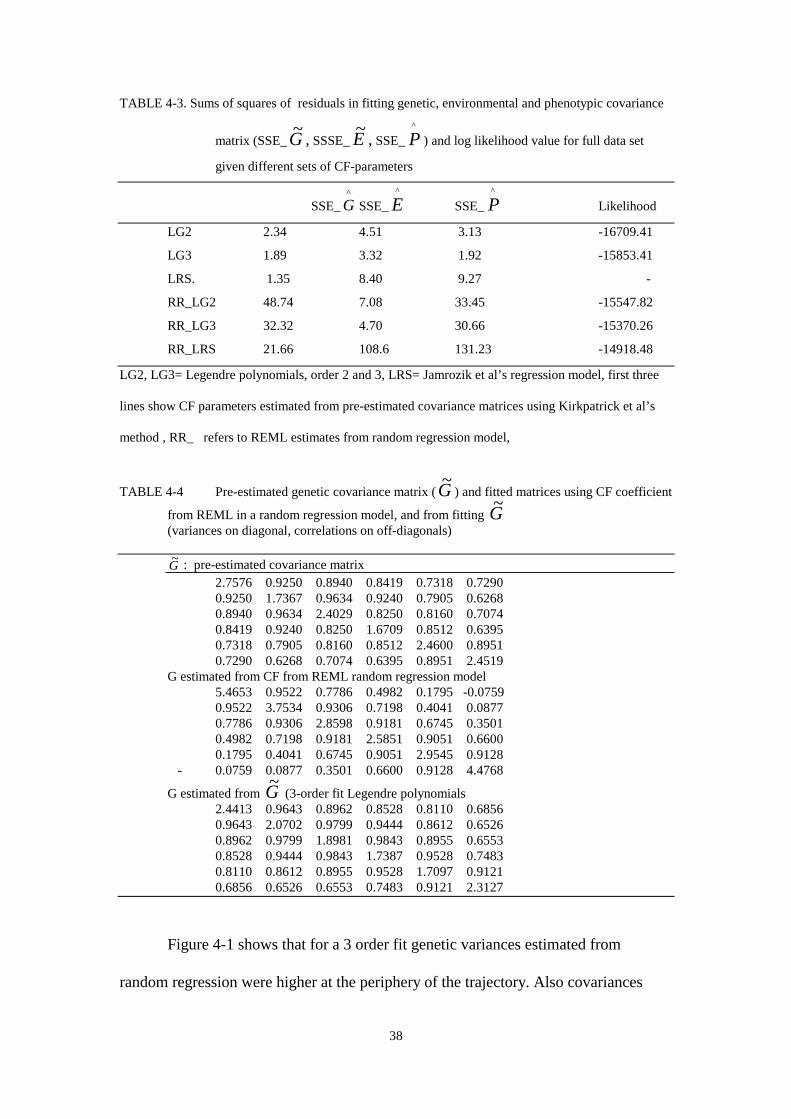
TABLE 4-3. Sums of squares of residuals in fitting genetic, environmental and phenotypic covariance
matrix (SSE_~G , SSSE_
~E , SSE_ P
^
) and log likelihood value for full data set
given different sets of CF-parameters
SSE_ G^
SSE_ E^
SSE_ P^
Likelihood
LG2 2.34 4.51 3.13 -16709.41
LG3 1.89 3.32 1.92 -15853.41
LRS. 1.35 8.40 9.27 -
RR_LG2 48.74 7.08 33.45 -15547.82
RR_LG3 32.32 4.70 30.66 -15370.26
RR_LRS 21.66 108.6 131.23 -14918.48
LG2, LG3= Legendre polynomials, order 2 and 3, LRS= Jamrozik et al’s regression model, first three
lines show CF parameters estimated from pre-estimated covariance matrices using Kirkpatrick et al’s
method , RR_ refers to REML estimates from random regression model,
TABLE 4-4 Pre-estimated genetic covariance matrix (~G ) and fitted matrices using CF coefficient
from REML in a random regression model, and from fitting ~G
(variances on diagonal, correlations on off-diagonals)
~G : pre-estimated covariance matrix2.7576 0.9250 0.8940 0.8419 0.7318 0.7290
0.9250 1.7367 0.9634 0.9240 0.7905 0.6268 0.8940 0.9634 2.4029 0.8250 0.8160 0.7074 0.8419 0.9240 0.8250 1.6709 0.8512 0.6395 0.7318 0.7905 0.8160 0.8512 2.4600 0.8951 0.7290 0.6268 0.7074 0.6395 0.8951 2.4519
G estimated from CF from REML random regression model5.4653 0.9522 0.7786 0.4982 0.1795 -0.0759
0.9522 3.7534 0.9306 0.7198 0.4041 0.0877 0.7786 0.9306 2.8598 0.9181 0.6745 0.3501 0.4982 0.7198 0.9181 2.5851 0.9051 0.6600 0.1795 0.4041 0.6745 0.9051 2.9545 0.9128 - 0.0759 0.0877 0.3501 0.6600 0.9128 4.4768
G estimated from ~G (3-order fit Legendre polynomials
2.4413 0.9643 0.8962 0.8528 0.8110 0.6856 0.9643 2.0702 0.9799 0.9444 0.8612 0.6526 0.8962 0.9799 1.8981 0.9843 0.8955 0.6553 0.8528 0.9444 0.9843 1.7387 0.9528 0.7483 0.8110 0.8612 0.8955 0.9528 1.7097 0.9121 0.6856 0.6526 0.6553 0.7483 0.9121 2.3127
Figure 4-1 shows that for a 3 order fit genetic variances estimated from
random regression were higher at the periphery of the trajectory. Also covariances

39
between ages most far apart were more extreme in the CF estimated from RR model.
Genetic correlation between the first and the last month of lactation was near zero
with the CF from the RR model, whereas it was near 0.7 in a bivariate analysis (Table
4-4).
From this comparison, it appears that estimating CF parameters from a random
regression model may not always give reliable parameters. In our example,
particularly genetic variance was overpredicted near the edges. From this analysis it is
hard to generalize this as being a property of random regression models, and more
work is needed in this area. For example, the REML program may have had problems
in finding a global maximum. The problem appeared to be worse for models with
regression on Legendre polynomials, and it is known that polynomial regression can
behave suboptimal near the edges (K. Meyer, pers. comm.). Figure 4-2 shows that
Jamrozik et al’s lactation curve model did not have this problem to the same extent.
For this reason, polynomial regression may be less suitable for estimating CF .
However, also the latter model deviated more from ~G than expected and correlation
between first and last lactation periods were also near zero.
An argument against estimating CF parameters from RR models is that
estimation of the CF for one random effect depends on the order of fit for other
random effects, since the likelihood of the data is maximized given one particular
model for all random effects. For example, Jamrozik et al’s model estimated with the
RR procedure was fitted with a constant permanent environmental variance (order of
fit=1), whereas fitting ~G with Kirkpatrick et al’s method basically assumed a high
dimensional fit (order = 6) for the environmental variances.
The conclusion is that although it is theoretically most appealing to
estimate CF parameters directly from a random regression model, this method may not
always give the most reliable estimates. More work needs to be done in this area,
including testing of other estimation methods (e.g. Gibbs sampling), other regression

40
techniques (e.g. the use of splines), and other statistical models (e.g. varying the
temporary environmental variance along the trajectory). The method of Kirkpatrick et
al involves much less computational effort than fitting a random regression model
(unless ~G and
~P are estimated between many ages), particularly when comparing
several order’s of fit for several random effects. Furthermore, it is easier to test more
complex covariance functions, like Veerkamp et al (1997) who tested a two
dimensional CF with the variance being a function of lactation stage as well as from
production level (see Chapter 5).
0
2
4
6
8
10
12
14
0 30
60
90
120
150
180
210
240
270
300
vari
ance
(kg
2)
Va_CF
Va_RR
Vc_CF
Vc_RR
VP_CF
VP_RR
Figure 4-1 Phenotypic, additive genetic and permanent environmental variances over lactation
estimated by covariance function (3-order Legendre polynomials) from multiple trait variance-
covariance matrices (CF) and by REML directly from data (RR)

41
0
1
2
3
4
5
6
7
80 15
30
45
60
75
90
105
120
135
150
165
180
195
210
225
240
255
270
285
300
days in milk
vari
ance
(kg
2)
Va_CF
Va_RR
Va-RRLrs
Figure 4-2 Additive genetic variance over lactation estimated by covariance function (3-order Legendre
polynomials) from multiple trait variance-covariance matrices (Va-CF) and by REML directly
from data (Va-RR) and with the Jamrozik et al’s model (Va-RRLrs)

42
6 Analyzing patterns of variation
Kirkpatrick and Heckman (1989) and Kirkpatrick et al (1990) show that covariance
functions can be used to analyze ‘patterns of inheritance’ in the covariance matrix ~G .
For this purpose they determined eigenvalues and eigenfunctions from the coefficient
matrix for a given covariance function.
In a way, this is a similar approach as principal component analysis. If we
consider the covariance structure among 25 type traits in dairy, we might be able to
say that one main eigenvalue is due to some kind of linear combination of all type
traits related to udder scores. We would find this if this is a group of traits highly
correlated among each other, but not highly correlated to other traits. In the canonical
decomposition of covariance functions, determining such major components has an
special meaning, because it shows at which ages the observed variables are correlated,
and where they are not. In other words, it shows how independent variables act on the
trait along the trajectory. For example we may determine that a first major eigenvalue
is related to a linear combination of test days in the first part of lactation (the
combination being defined by the eigenvector attached to that eigenvalue), whereas
another eigenvalue may be a combination of test day variables in later lactation. If this
was found for the genetic covariance matrix, the interpretation could be that two main
and independent components could be distinguished in milk production, each acting
on different parts of lactation, and those two components could be related to different
genes, possible on two different parts of the genome. The last would be of interest in
QTL analysis: one canonical variable could be linked to one marker, whereas another
is linked to another marker.
In contrast to multiple traits, the variables in repeated measurement can be
ordered along a trajectory. In that case, The transformation of variables described by
each eigenvector can be written as a continuous function of age. This is indicated as
eigenfunction (Kirkpatrick and Heckman, 1989). Eigenfunctions are calculated as
follows:
Consider the covariance function
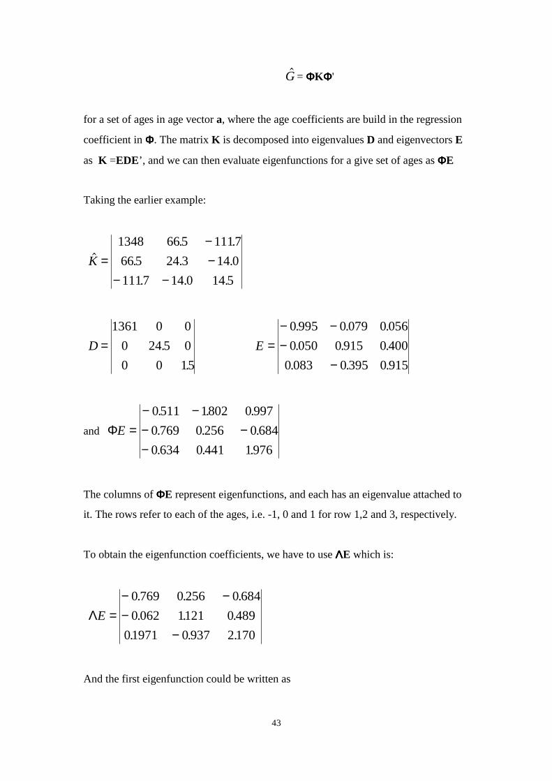
43
!G = ΦΦΦΦKΦΦΦΦ'
for a set of ages in age vector a, where the age coefficients are build in the regression
coefficient in ΦΦΦΦ. The matrix K is decomposed into eigenvalues D and eigenvectors E
as K =EDE’, and we can then evaluate eigenfunctions for a give set of ages as ΦΦΦΦE
Taking the earlier example:
!. .
. . .
. . .
K =−−
− −
1348 665 1117
665 24 3 14 0
1117 14 0 14 5
D =1361 0 0
0 24 5 0
0 0 15
.
.
E =− −−
−
0 995 0 079 0 056
0 050 0 915 0 400
0 083 0 395 0 915
. . .
. . .
. . .
and ΦE =− −− −−
0511 1802 0 997
0 769 0 256 0 684
0 634 0 441 1976
. . .
. . .
. . .
The columns of ΦΦΦΦE represent eigenfunctions, and each has an eigenvalue attached to
it. The rows refer to each of the ages, i.e. -1, 0 and 1 for row 1,2 and 3, respectively.
To obtain the eigenfunction coefficients, we have to use ΛΛΛΛE which is:
ΛE =− −−
−
0 769 0 256 0 684
0 062 1121 0 489
01971 0 937 2170
. . .
. . .
. . .
And the first eigenfunction could be written as

44
ψ1
20 769 0 062 0197( ) . . .x x x= − − +
Figure 4 shows the three eigenfunction plotted for the example of Kirkpatrick et al.
(1990). It should be noticed that the sign a the evaluated values between
eigenfunctions is irrelevant (for example, the firs eigenfunction has only positive
values in the Genetics paper of Kirkpatrick et al. What matter is how the values of the
eigenfunctions change over the trajectory. In this example, the main eigenfunction is
almost constant for all ages. Since it has the largest eigenvalues attached to it, the
interpretation is that the major part of the genetic variance is explained by a factor that
is constant for all ages. Selection on this factor will increase weight for all ages. Since
this eigenvalue is very dominant, selection for weight at any age will improve weight
on all ages. In multiple trait terms, weight at different ages is highly correlated (from
the G used in the example, we can calculate correlations of 0.88 between weight at 2
and 3 weeks; o.86 between weight at 2 and 4 weeks ,and 0.99 between weight at 3
and 4 weeks.
eigenfuctions kirkpatrick example
-2
-1.5
-1
-0.5
0
0.5
1
1.5
2
1 3 5 7 9 11
13
15
17
19
21
23
25
27
29
31
age
1361
24.5
1.5
Figure 4 Eigenfunctions for the example of Kirkpatrick et al (1990)
A very interesting pattern is shown by the second eigenfunction. Selection on this
variable decreases weight at early age and increases weight at later ages. Selection on
the variable represented by this eigenfunction could therefore be used to change the
growth curve, e.g. select for lower weight at start and higher weight at the end of a
trajectory considered. In this example, the 2nd and 3rd eigenvalues are not very large
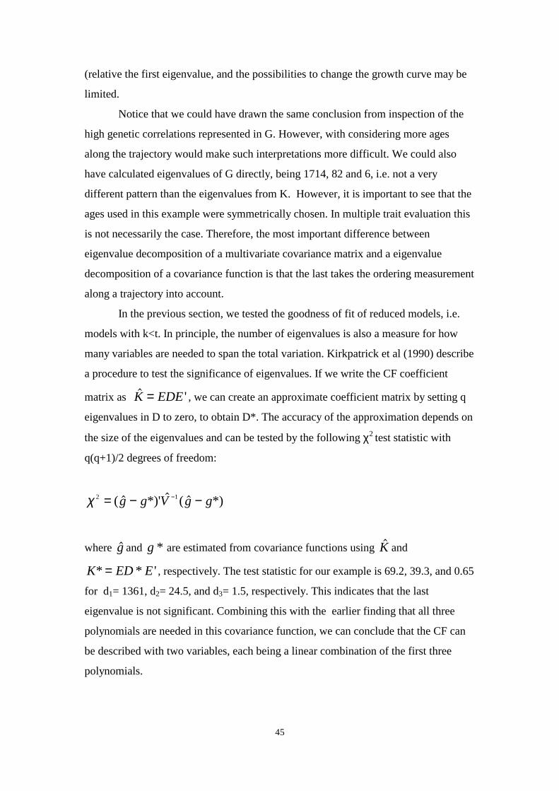
45
(relative the first eigenvalue, and the possibilities to change the growth curve may be
limited.
Notice that we could have drawn the same conclusion from inspection of the
high genetic correlations represented in G. However, with considering more ages
along the trajectory would make such interpretations more difficult. We could also
have calculated eigenvalues of G directly, being 1714, 82 and 6, i.e. not a very
different pattern than the eigenvalues from K. However, it is important to see that the
ages used in this example were symmetrically chosen. In multiple trait evaluation this
is not necessarily the case. Therefore, the most important difference between
eigenvalue decomposition of a multivariate covariance matrix and a eigenvalue
decomposition of a covariance function is that the last takes the ordering measurement
along a trajectory into account.
In the previous section, we tested the goodness of fit of reduced models, i.e.
models with k<t. In principle, the number of eigenvalues is also a measure for how
many variables are needed to span the total variation. Kirkpatrick et al (1990) describe
a procedure to test the significance of eigenvalues. If we write the CF coefficient
matrix as ! 'K EDE= , we can create an approximate coefficient matrix by setting q
eigenvalues in D to zero, to obtain D*. The accuracy of the approximation depends on
the size of the eigenvalues and can be tested by the following χ2 test statistic with
q(q+1)/2 degrees of freedom:
χ 2 1= − −−( ! *)' ! ( ! *)g g V g g
where !g and g * are estimated from covariance functions using !K and
K ED E* * '= , respectively. The test statistic for our example is 69.2, 39.3, and 0.65
for d1= 1361, d2= 24.5, and d3= 1.5, respectively. This indicates that the last
eigenvalue is not significant. Combining this with the earlier finding that all three
polynomials are needed in this covariance function, we can conclude that the CF can
be described with two variables, each being a linear combination of the first three
polynomials.

46
7 Summarizing Discussion
We have presented various ways to analyze repeated measurements where interest is
in a model that uses correct variance covariance structures between the observations,
and that can make use and enable inferences on the gradual change of the
measurements over time. A random regression model seems the most appropriate for
modeling such data, and such models more or less implicitly use covariance functions.
Canonical transformation can be used to simplify large scale genetic evaluations, and
to reduce the rank of the covariance matrices used for each random effect. Eigenvalue
decomposition possibly reveal patterns in the covariance structure, and might be of
help to implement selection rules that aim for a change of the curves. Such analysis
might also be useful when detecting more specifically the mode of action of
Quantitative Trait Loci in specific parts of the genome, determined by genetic
markers, or to identify parts of genetic variation that are specifically correlated with
third traits of interest. Such analysis has similarities with principal component
analysis, but the extra dimension is added by considering principal components as a
function of time (eigenfunctions).
In the previous chapters the use of covariance functions was discussed in a
general sense, and with particular emphasis on application to analysis of test day
models. Another area where covariance functions and random regression models can
be applied to is the analysis of weight and growth data, feed intake, etc. Trait
measurements can e modeled as a function of time, but also as a function of a
continuous environmental variable (herd production level, ambient temperature, etc).
For example genetic variation in susceptibility to heat can be modeled by regression
production on a heat stress index (a function of temperature and humidity). Variation
in susceptibility to disease can be measures as a regression of parasite infection level
on an environmental variable that measures environmental risk to disease.
Many studies have considered genetic aspects of growth by first estimating parameters
for growth curves, and subsequently estimating variance components for the growth
curve parameters. Such analysis could be improved upon by the use of random
regression models. Main differences between these approaches is that the first (two-
47
step) approach maybe less able to estimate curves for animals with missing data, and
more general, does not use information from relatives. The values of such information
is well known to animal breeders, not only in gaining accuracy, but also to account for
directional selection. Varona et al (1997) presented random regression models in a
Bayesian manner, and give a good discussion on the merits of such models over the
two-step procedure with first estimating curve parameters and subsequently estimating
their variance components.
It is often of interest not only to analyze the behavior of a repeatedly measured
trait over time as such, but also to study correlations of certain curve parameters with
‘third’ traits. An example is to study growth curves by random regression models for
weight data, and to correlate CF parameters with meat quality traits such as fat and
muscle. Animals that tend to grow faster in the last phase before slaughter may have
also a different pattern for onset of body fat, different mature weight and a different
maturity rate (age at first calving!). Multivariate random regression analyses are
required here. Such analyses will form a computational challenge (with a need to
explore robustness of the estimation) but will be the basis of a very interesting
biological debate on how to improve such dynamic traits of growth and development
such that animals will have improved prformance in the prevailing production system.
Remaining points of debate on the use of random regression models, and
further research will be predominantly focused on the specific regression models used
for fitting covariance structures. Two approaches are to choose a regression equation
that was developed to model the mean curve (growth curve, lactation cure) and take
regression coefficients random . The other approach is to fit the covariance structure
by polynomial regression, or alternatively by splines. Fitting a curve with many
parameters will generally give an accurate fit of the covariance structure. However,
there is often an interest in fewer numbers of parameters. Models based on ‘biological
curves’ may appeal because certain parameters have a ‘biological meaning’. However,
the biological meaning from polynomials can be determined by plotting
eigenfunctions from polynomials. Lindsey (1993) argues that it is generally preferable
to choose a model that describes the mechanism that generates the data. Herewith, we
can refer to modeling certain residual covariance matrices, which may have
autocorrelation structures. Lindsey also discusses growth curves and refer to

48
Sandland and McGilchrist (1979) who provide a number of reasons why polynomials
are unattractive for growth models:
1) growth processes can undergo changes of phase which cannot be accommodated
by polynomials
2) the stochastic structure of the model will be distorted if the polynomial is
inappropriate
3) polynomials cannot easily represent asymptotic behavior of a growth curve.
Anderson and Pedersen (1996) argue that many growth curves are non-linear
functions (e.g. Gompertz, logistic regression) for which is more difficult to introduce
random effects. They also argue that average curves of the exponential form (e.g. y= a
exp(-bx-c/x) are not of the same form if the parameters a, b and c vary from animal to
animal. Sometimes, transformations to linear models are possible, although
transformations to stabilize between animal variation may destabilize within animal
variation (see Anderson and Pedersen (1997) for an example).
The need to avoid polynomials depends on the trajectory considered. In certain
instances, it may be more important to accurately account for asymptotes, in which
case polynomials are less appropriate. The use of splines is often advocated as being a
robust technique in regression analysis and should probably be considered as very
useful in random regression analysis as well. Also, the behavior of different random
regression models in relation to data structure needs more study. For some traits, there
may be many more data point at the younger ages, and there may be sequential
selection. In general, estimating covariance matrices between certain ages of the
trajectory can be useful as a reference for checking parameter estimates for covariance
functions, as was also demonstrated in these notes.
In general, arguments for fitting mean growth curves for populations, or
subpopulations, can also be used for random regression models. The same holds true
for the number of parameters that should be used to fit regression models. However, a
practical argument for analyzing (large size) animal breeding data is that more random
regression coefficients rapidly increase computing demands, and that for predicting
breeding values, accurately fitting first moments (means) is usually more important
than accurately fitting second moments (variances)

49

50
References
Anderson, S, and Pedersen, B. 1996. Growth curve and food intake curves for grouphoused gilts and castrated male pigs. Animal Sci. 63:457-464.
Diggle, P.J., Liang, K.-Y. and Zeger, S.L. 1994. Analysis of longitudinal data.Clarendon Press, Oxford.
Ducrocq, V.P., and Besbes. 1993. Solution of multiple trait animal models withmissing data on some traits. J. Anim. Breed. Genet. 110:81-92.
Hayes, J.F. and Hill, W.G., 1981. Modification of estimates of parameters in theconstruction of genetic selection indices (‘bending’) Biometrics 37:483-493.
Jamrozik, J. and L.R. Schaeffer. 1997. Estimates of genetic parameters for a test daymodel with random regressions for production of first lactation Holsteins. J.Dairy Sci. (in press).
Johnson, D.L. and Thompson, R. 1995. Restricted maximum Likelihood estimation ofvariance components for univariate animal models using sparse matrixtechniques and average information. J. Dairy Sci. 78_449-456.
Kirkpatrick, M., Lofsvold, D., and Bulmer, M. 1990. Analysis of the inheritance,selection and evolution of growth trajectories. Genetics 124:979-993.
Kirkpatrick, M., Thompson, R., and Hill, W.G. 1994. Estimating the covariancestructure of traits during growth and ageing, illustrated with lactation in dairycattle. Genetical Research 64:57-69.
Lindsey, J.K. 1993. Models for repeated measurements. Clarendon Press, Oxford.Meyer, K, and Hill, W.G. 1997. Estimation of genetic and phenotypic covariance
functions for longitudinal or ‘repeated’ records by Restricted MaximumLikelihood. Livest. Prod. Sci. 47:185-200.
Meyer, K. 1997. Estimates of covariance functions for mature weight of beef cows inthe Wokalup selection experiment. Proc. Assoc. Advmt. Anim. Breed. Genet.
Meyer, K. 1997. Estimation of genetic and phenotypic covariance functions forlongitudinal data. Proc. Assoc. Advmt. Anim. Breed. Genet. 12: 534-537.
Meyer, K. DFREML and covariance functions with random regression. In preparationPtak, E., and L.R. Schaeffer. 1993. Use of test day yields for genetic evaluation in
dairy sires and cows. Livest. Prod. Sci. 34:23Sandland, R.L. and McGilchrist, C.A. 1979. Stochastic growth curve analysis.
Biometrics 35:255-271.Varona, L., Moreno, C, Carcia Cortes, L.A., and Altarriba, J. 1997. Multiple trait
genetic analysis of underlying biological variables of production functions.Livest. Prod. Sci. 47: 201-209.
Van der Werf, J.H.J., Goddard, M.E., and Meyer, K. 1997. The use of covariancefunctions and random regression for genetic evaluation of milk productionbased on test day records. (in preparation)
Veerkamp, R.F. and M.E. Goddard. 1997. Covariance functions across herdproduction levels for test day records on milk fat and protein yield. J. DairySci. (abstract).
Visscher, P.M. 1994. Bias in genetic R2 from half sib designs. Proc. 5th WCGALPGuelph.
Wiggans, G. and Goddard, M.E. 1997. Test day model with 30 traits and geneticcovariance matrix of reduced rank. J. Dairy Sci. In Press