4

Comparing Asset Pricing Models

Francisco Barillas and Jay Shanken*

Abstract

A Bayesian asset-pricing test is derived that is easily computed in closed-form from the

standard F-statistic. Given a set of candidate traded factors, we develop a related test procedure

that permits an analysis of model comparison, i.e., the computation of model probabilities for the

collection of all possible pricing models that are based on subsets of the given factors. We find

that the recent models of Hou, Xue and Zhang (2015a,b) and Fama and French (2015, 2016) are

both dominated by a variety of models that include a momentum factor, along with value and

profitability factors that are updated monthly.

                                                       * Barillas and Shanken are from the Goizueta Business School at Emory University. Shanken is also from the

National Bureau of Economic Research. Corresponding author: Jay Shanken, Goizueta Business School, Emory

University, 1300 Clifton Road, Atlanta, Georgia, 30322, USA; telephone: (404)727-4772; fax: (404)727-5238. E-

mail: jay.shanken@emory.edu. Thanks to two anonymous referees, Rohit Allena, Doron Avramov, Mark Fisher,

Amit Goyal, Lubos Pastor, Tim Simin, Ken Singleton (the editor), Rex Thompson, Pietro Veronesi and seminar

participants at the Northern Finance Association meeting, Southern Methodist University, the Universities of

Geneva, Hong Kong, Lausanne, Luxembourg and Singapore, Hong Kong University of Science and Technology,

Imperial College, National University of Singapore and Ohio State University.

 

5

Given the variety of portfolio-based factors that have been examined by researchers, it is

important to understand how best to combine them in a parsimonious asset-pricing model for

expected returns, one that excludes redundant factors. There are standard econometric techniques

for evaluating the adequacy of a single model, but a satisfactory statistical methodology for

identifying the best factor-pricing model(s) is conspicuously lacking in investment research

applications. We develop a Bayesian procedure that is easily implemented and allows us to

compute model probabilities for the collection of all possible pricing models that can be formed

from a given set of factors.

Beginning with the capital asset pricing model (CAPM) of Sharpe (1964) and Lintner

(1965), the asset pricing literature in finance has attempted to understand the determination of

risk premia on financial securities. The central theme of this literature is that the risk premium

should depend on a security’s market beta or other measure(s) of systematic risk. In a classic test

of the CAPM, Black, Jensen and Scholes (1972), building on the earlier insight of Jensen (1968),

examine the intercepts in time-series regressions of excess test-portfolio returns on market excess

returns. Given the CAPM implication that the market portfolio is efficient, these intercepts or

“alphas” should be zero. A joint F-test of this hypothesis is later developed by Gibbons, Ross

and Shanken (1989), henceforth GRS, who also explore the relation of the test statistic to

standard portfolio geometry.1

                                                       1 See related work by Treynor and Black (1973) and Jobson and Korkie (1982).

 

6

In recent years, a variety of multifactor asset pricing models have been explored. While

tests of the individual models are routinely reported, these tests often suggest “rejection” of the

implied restrictions, especially when the data sets are large, e.g., Fama and French (2016). On

the other hand, a relatively large p-value may say more about imprecision in estimating a

particular model’s alphas than the adequacy of that model.2 Sorely needed are simple statistical

tools with which to analyze the various models jointly in a model-comparison framework. This

is an area of testing that has received relatively little attention,  especially in the case of non-

nested models. The information that our methodology provides about relative model likelihoods

complements that obtained from classical asset-pricing tests and is more in the spirit of the

adage, “it takes a model to beat a model.” 3

Like other asset pricing analyses based on alphas, we require that the benchmark factors

are traded portfolio excess returns or return spreads. For example, in addition to the market

                                                       2 De Moor, Dhaene and Sercu (2015) suggest a calculation that highlights the extent to which differences in p-values

may be influenced by differences in estimation precision across models, but they do not provide a formal hypothesis

test.

3 Avramov and Chao (2006) also explore Bayesian model comparison for asset pricing models. As we explain in

the next two sections, their methodology is quite different from that developed here. A recent paper by Kan, Robotti

and Shanken (2013) provides asymptotic results for comparing model R2s in a cross-sectional regression framework.

Chen, Roll and Ross (1986) nest the CAPM in a multifactor model with betas on macro-related factors included as

well in cross-sectional regressions. In other Bayesian applications, Malatesta and Thompson (1993) apply methods

for comparing multiple hypotheses in a corporate finance event study context.

 

7

excess return, Mkt, the influential three-factor model of Fama and French (1993), hereafter, FF3,

includes a book-to-market or “value” factor HML (high-low) and a size factor, SMB (small-big)

based on stock-market capitalization. Although consumption growth and intertemporal hedge

factors are not traded, one can always substitute (maximally correlated) mimicking portfolios for

the non-traded factors.4 While this introduces additional estimation issues, simple spread-

portfolio factors are often viewed as proxies for the relevant mimicking portfolios, e.g., Fama

and French (1996).

We begin by analyzing the joint alpha restriction for a set of test assets in a Bayesian

setting.5 Prior beliefs about the extent of model mispricing are economically motivated and

accommodate traditional risk-based views as well as more behavioral perspectives. The

posterior probability that the zero-alpha restriction holds is then shown to be an easy-to-calculate

function of the GRS F-statistic. Our related model-comparison methodology is likewise

computationally straightforward. This procedure builds on results in Barillas and Shanken

(2017), who highlight the fact that for several widely accepted criteria, model comparison with

traded factors only requires an examination of each model’s ability to price the factors in the

other models.

It is sometimes observed that all models are necessarily simplifications of reality and

hence must be false in a literal sense. This motivates an evaluation of whether a model holds

                                                       4 See Merton (1973) and Breeden (1979), especially footnote 8.

5 See earlier work by Shanken (1987b), Harvey and Zhou (1990) and McCulloch and Rossi (1991).

 

8

approximately, rather than as a sharp null hypothesis. Additional motivation comes from

recognizing that the factors used in asset-pricing tests are generally proxies for the relevant

theoretical factors.6 With these considerations in mind, we extend our results to obtain simple

formulas for testing the more plausible approximate models.

As a warm up, we consider all models that can be obtained using subsets of the FF3

factors, Mkt, HML and SMB. A nice aspect of the Bayesian approach is that it permits

comparison of nested models like CAPM and FF3, as well the non-nested models {Mkt HML}

and {Mkt SMB}. Moreover, we are able to simultaneously compare all of the models, as

opposed to standard classical approaches, e.g., Vuong (1989), that involve pairwise model

comparison. Over the period 1972-2015, alphas for HML when regressed on either Mkt or Mkt

and SMB are highly “significant,” whereas the alphas for SMB when regressed on Mkt or Mkt

and HML are modest. Our procedure aggregates all of this evidence, arriving at posterior

probabilities of 60% for the two-factor model {Mkt HML} and 39% for FF3, with the remaining

1% split between CAPM and {Mkt, SMB}.

In our main empirical application, we compare models that combine many prominent

factors from the literature. In addition to the FF3 factors, we consider the momentum factor,

UMD (up minus down), introduced by Carhart (1997) and motivated by the work of Jegadeesh

and Titman (1993). We also include factors from the recently proposed five-factor model of

                                                       6 Kandel and Stambaugh (1987) and Shanken (1987a) analyze pricing restrictions based on proxies for the market

portfolio or other equilibrium benchmark.

 

9

Fama and French (2015), hereafter FF5.7 These are RMW (robust minus weak), based on the

profitability of firms, and CMA (conservative minus aggressive), related to firms’ net

investments. Hou, Xue and Zhang (2015a, 2015b), henceforth HXZ, have proposed their own

versions of the size (ME), investment (IA) and profitability (ROE) factors, which we also

examine. In particular, ROE incorporates the most recent earnings information from quarterly

data. Finally, we consider the value factor HMLm from Asness and Frazzini (2013), which is

based on book-to-market rankings that use the most recent monthly stock price in the

denominator. In total, we have ten factors in our analysis.

Rather than mechanically apply our methodology with all nine of the non-market factors

treated symmetrically, we structure the prior so as to recognize that several of the factors are just

different versions of the same underlying construct. Therefore, to avoid overfitting, we only

consider models that contain at most one version of the factors in each category: size (SMB or

ME), profitability (RMW or ROE), value (HML or HMLm) and investment (CMA or IA). The

extension of our procedure to accommodate such “categorical factors” amounts to averaging

results over the different versions of the factors, with weights that reflect the likelihood that each

version contains the relevant factors.

Using data from 1972 to 2015 we find that the individual model with highest posterior

probability is the six-factor model {Mkt IA ROE SMB HMLm UMD}. Thus, in contrast to

                                                       7 We use the SMB factor from the FF5 model in this paper. Our findings are not sensitive to whether we use the

original SMB, as the correlation between the two size measures is over 0.99.

 

10

previous findings by HXZ and FF5, value is no longer a redundant factor when the more timely

version HMLm is considered; and whereas HXZ also found momentum redundant, this is no

longer true with inclusion of HMLm. The timeliness of the HXZ profitability factor turns out to

be important as well. The other top models are closely related to our best model, replacing SMB

with ME, IA with CMA, or excluding size factors entirely. There is also overwhelming support

for the six-factor model (or the five-factor model that excludes SMB) in direct tests of the model

against the HXZ and FF5 models. These model-comparison results are qualitatively similar for

priors motivated by a market-efficiency perspective and others that allow for large departures

from efficiency. The models identified as best in the full-sample Bayesian analysis perform well

out-of sample, but so do the HXZ and FF5 models.

Model comparison assesses the relative performance of competing models. We also

examine absolute performance for the top-ranked model. This test considers the extent to which

the model does a good job of pricing a set of test assets. Although various test assets were

examined, results are presented for two sets: 25 portfolios based on independent rankings by

either size and momentum or by book-to-market and investment. This evidence casts strong

doubt on the validity of our six-factor model. The “rejection” is less overwhelming, however,

when an approximate version is considered that allows for relatively small departures (average

absolute value 0.8% per annum) from exact pricing.

The rest of the paper is organized as follows. Section I considers the classic case of

testing a pricing model against a general alternative. Section II then considers the comparison of

 

11

nested pricing models and the relation between “relative” and “absolute” tests. Bayesian model

comparison is analyzed in Section III. Section IV extends the model-comparison framework to

accommodate analysis with multiple versions of some factors. Section V provides empirical

results for various pricing models based on ten prominent factors, while Section VI explores the

out-of-sample performance of our high-probability models, along with several other models from

the literature. Section VII examines the absolute performance of the model with the highest

probability. Section VIII concludes. Several proofs of key results are provided in an appendix,

along with an extension that treats the market symmetrically with the other factors. An internet

appendix with additional technical details is also available.

I. Testing a Pricing Model Against a General Alternative

Traditional tests of factor-pricing models compare a single restricted asset-pricing model

to an unrestricted alternative return-generating process that nests the null model. We explore the

Bayesian counterpart of such a test in this section.

A. Statistical Assumptions and Portfolio Algebra

First, we lay out the factor model notation and assumptions. The factor model is a

multivariate linear regression with N test-asset excess returns, tr , and K factors, for each of T

months:

t t t tr f ~ N(0, ),                                                                  (1) 

 

12

where tr , t  and are Nx1, is NxK and tf is Kx1. The normal distribution of the t is assumed

to hold conditional on the factors and the t are independent over time.

We assume that the factors are zero-investment returns such as the excess return on the

market or the spread between two portfolios, like the Fama-French value-growth factor. Under

the null hypothesis, 0H : 0 , we have the usual simple linear relation between expected

returns and betas:

t tE(r ) E(f ) , (2)

where tE(f ) is the Kx1 vector of factor premia.

The GRS test of this null hypothesis is based on the F-statistic with degrees of freedom N

and T-N-K, which equals (T-N-K)/(NT) times the Wald statistic:

1

2

ˆˆ ˆ'W T

1 Sh(F)

(3)

where

1 2 2ˆˆ ˆ' Sh(F, R) Sh(F) . (4)

Here, 2Sh(F) is the maximum squared sample Sharpe ratio over portfolios of the factors, where

is the maximum likelihood estimate (MLE) for the covariance matrix . The term

2Sh(F,R) is the squared Sharpe measure based on both factor and asset returns. The population

 

13

counterpart of the identity in (4) implies that the tangency portfolio corresponding to the factor

and asset returns equals that based on the factors alone under the null 0 . Thus, the expected

return relation in (2) is equivalent to this equality of tangency portfolios and their associated

squared Sharpe ratios.

B. A Bayesian Test of Efficiency

Bayesian tests of the zero-alpha restriction have been developed by Shanken (1987b),

Harvey and Zhou (1990) and McCulloch and Rossi (1991). The test that we develop here takes,

as a starting point, a prior specification considered in the Harvey and Zhou paper. Although they

comment on the computational challenges of implementing this approach, we are able to derive a

simple closed-form formula for the required Bayesian probabilities. The specification is

appealing in that standard “diffuse” priors are used for the betas and residual covariance

parameters. Thus, the data dominate beliefs about these parameters, freeing the researcher to

focus on informative priors for the alphas, the parameters that are restricted by the models.8 The

details are as follows.

B.1 Prior Specification

The diffuse prior for and is

                                                       8 Using improper (diffuse) priors for “nuisance parameters” like betas and residual covariances that appear in both

the null and alternative models, but proper (informative) priors under the alternative for parameters like alpha, is in

keeping with Jeffreys (1961) and others.

 

14

( N 1)/2

P( , ) , (5)

as in Jeffreys (1961). The prior for is con centrated at 0 under the null hypothesis. Under the

alternative, we assume a multivariate normal informative prior for conditional on and :

, (6)

where the parameter k > 0 reflects our belief about the potential magnitude of deviations from

the expected return relation.

Asset-pricing theory provides some motivation for linking beliefs about the magnitude of

alpha to residual variance. For example, Dybvig (1983) and Grinblatt and Titman (1983) derive

bounds on an individual asset’s deviation from a multifactor pricing model that are proportional

to the asset’s residual variance. From a behavioral perspective, Shleifer and Vishny (1997) argue

that high idiosyncratic risk can be an impediment to arbitraging away expected return effects due

to mispricing. Pastor and Stambaugh (2000) also adopt a prior for with covariance matrix

proportional to the residual covariance matrix. Building on ideas in McKinlay (1995), they

stress the desirability of a positive association between and in the prior, which makes

extremely large Sharpe ratios less likely, as implied by (4).9

A very high Sharpe ratio can be viewed as an approximate arbitrage opportunity (see

Shanken (1992)) in that a substantial return is expected with relatively little risk. It can also be

                                                       9 Also see related work by Pastor and Stambaugh (1999) and Pastor (2000).

P( | , ) MVN(0, k )

 

15

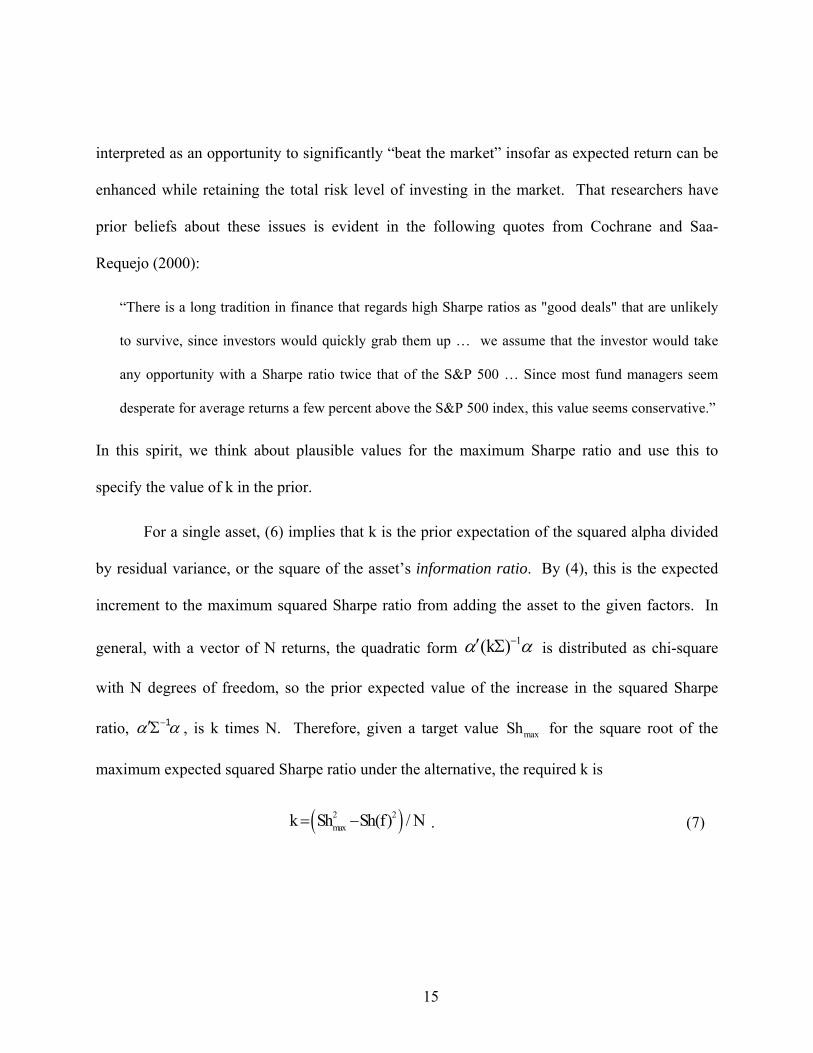
interpreted as an opportunity to significantly “beat the market” insofar as expected return can be

enhanced while retaining the total risk level of investing in the market. That researchers have

prior beliefs about these issues is evident in the following quotes from Cochrane and Saa-

Requejo (2000):

“There is a long tradition in finance that regards high Sharpe ratios as "good deals" that are unlikely

to survive, since investors would quickly grab them up … we assume that the investor would take

any opportunity with a Sharpe ratio twice that of the S&P 500 … Since most fund managers seem

desperate for average returns a few percent above the S&P 500 index, this value seems conservative.”

In this spirit, we think about plausible values for the maximum Sharpe ratio and use this to

specify the value of k in the prior.

For a single asset, (6) implies that k is the prior expectation of the squared alpha divided

by residual variance, or the square of the asset’s information ratio. By (4), this is the expected

increment to the maximum squared Sharpe ratio from adding the asset to the given factors. In

general, with a vector of N returns, the quadratic form 1(k ) is distributed as chi-square

with N degrees of freedom, so the prior expected value of the increase in the squared Sharpe

ratio, 1 , is k times N. Therefore, given a target value for the square root of the

maximum expected squared Sharpe ratio under the alternative, the required k is

. (7)

maxSh

2 2

maxk Sh Sh(f) / N

 

16

For example, in a test of the CAPM, = 2.0 times the market ratio of 0.115 implies that k is

(2.02-1)(0.1152)/10 = 0.004 when there are 10 test assets.10 As an alternative to this investment

perspective on the prior, we can focus directly on the expected return relation and our assessment

of plausible deviations from that relation. This is similar to the approach in Pastor (2000).

One may wonder why we don’t consider a diffuse prior for alpha, so as to avoid having to

make an assumption about the prior parameter k. In some contexts, a diffuse prior can be

obtained in the limit by letting the prior variance approach infinity. Allowing → ∞ here

would amount to letting k → ∞, which is not sensible economically since it implies, by (7), that

the maximum squared Sharpe ratio expected under the alternative is itself infinite. That some

form of informative prior is required for alpha follows more generally from observations in a

widely cited article on Bayes factors by Kass and Raftery (1995). They discuss the relevance of

“Bartlett’s (1957) paradox,” a situation in which an estimate may be far from its null value, but

even more unlikely under the alternative, thus yielding a Bayes factor that favors the null H0. A

consequence, they note, is that a prior under the alternative with a large variance will “force the

Bayes factor to favor H0.” They attribute this point to Jeffreys (1961), who recognizes that, “to

avoid this difficulty, priors on parameters being tested must be proper and not have too big a

spread.” What this means in our application is that, in evaluating an asset pricing model, a

                                                       10 Note that using the factor data to inform the prior is appropriate in this context since the entire statistical analysis

is conditioned on f.

maxSh

 

17

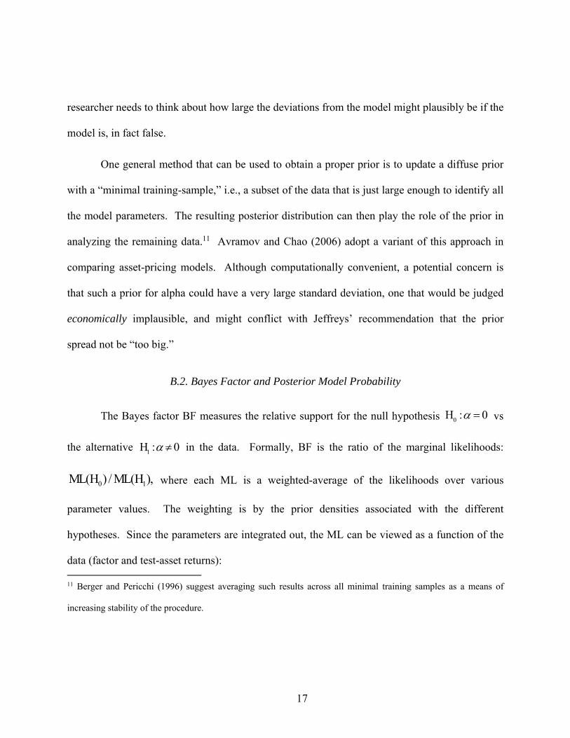
researcher needs to think about how large the deviations from the model might plausibly be if the

model is, in fact false.

One general method that can be used to obtain a proper prior is to update a diffuse prior

with a “minimal training-sample,” i.e., a subset of the data that is just large enough to identify all

the model parameters. The resulting posterior distribution can then play the role of the prior in

analyzing the remaining data.11 Avramov and Chao (2006) adopt a variant of this approach in

comparing asset-pricing models. Although computationally convenient, a potential concern is

that such a prior for alpha could have a very large standard deviation, one that would be judged

economically implausible, and might conflict with Jeffreys’ recommendation that the prior

spread not be “too big.”

B.2. Bayes Factor and Posterior Model Probability

The Bayes factor BF measures the relative support for the null hypothesis vs

the alternative in the data. Formally, BF is the ratio of the marginal likelihoods:

0 1ML(H ) / ML(H ), where each ML is a weighted-average of the likelihoods over various

parameter values. The weighting is by the prior densities associated with the different

hypotheses. Since the parameters are integrated out, the ML can be viewed as a function of the

data (factor and test-asset returns):                                                        11 Berger and Pericchi (1996) suggest averaging such results across all minimal training samples as a means of

increasing stability of the procedure.

0H : 0

1H : 0

 

18

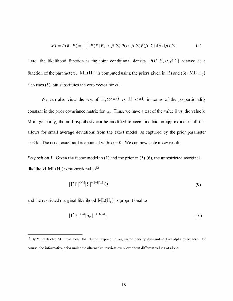
( | ) ( | , , , ) ( | , ) ( , ) d d d . ML P R F P R F P P (8)

Here, the likelihood function is the joint conditional density ( | , , , ) P R F viewed as a

function of the parameters. 1ML(H ) is computed using the priors given in (5) and (6); 0ML(H )

also uses (5), but substitutes the zero vector for .

We can also view the test of 0H : 0 vs 1H : 0 in terms of the proportionality

constant in the prior covariance matrix for . Thus, we have a test of the value 0 vs. the value k.

More generally, the null hypothesis can be modified to accommodate an approximate null that

allows for small average deviations from the exact model, as captured by the prior parameter

k0 < k. The usual exact null is obtained with k0 = 0. We can now state a key result. 

Proposition 1. Given the factor model in (1) and the prior in (5)-(6), the unrestricted marginal

likelihood is proportional to12

N/2 (T K)/2| FF| |S| Q (9)

and the restricted marginal likelihood is proportional to

N/2 (T K)/2R| F F| |S | , (10)

                                                       12 By “unrestricted ML” we mean that the corresponding regression density does not restrict alpha to be zero. Of

course, the informative prior under the alternative restricts our view about different values of alpha.

1ML(H )

0ML(H )

 

19

where S and SR are the NxN cross-product matrices of the OLS residuals with unconstrained

or constrained to equal zero, respectively. The scalar Q is given by

1 //

1/

, (11)

where 2a 1 Sh(F) / T . W is given in (3) and equals the GRS F-statistic times NT/(T-N-K).

Therefore, the Bayes factor for vs equals

(T K)/2

0

1 R

SML(H ) 1BF

ML(H ) Q S

.            (12)

Letting Qk0 be the value of Q obtained with prior value k0, the BF for k0 vs k is

0 0k ,k kBF Q / Q . (13)

Proof. See Appendix B.13, 14

Consistent with intuition, the marginal likelihoods increase with the fit of each model,

which is inversely related to the OLS residual sum of squares (unrestricted or restricted).

However, it is well known from classical statistics that the fit implied by the OLS estimates

                                                       13 Harvey and Zhou derive (12) in the univariate case, with a complicated integral expression for Q. The function of

W in (11) is our simplification, while (13) is both a further simplification and generalization of (12).

14 The formula is identical, apart from minor differences in notation, to the Bayes factor that Shanken (1987b)

derives by conditioning directly on the F-statistic, rather than on all the data, for simplicity. Thus, surprisingly, it

turns out that this simplification entails no loss of information under the diffuse prior assumptions made here.

0H : 0 1H : 0

 

20

overstates the true fit.15 In Proposition 1, the presence of the F F term in the MLs can be traced

back algebraically to this fact. It amounts to a prior-weighted adjustment of fit to reflect

measurement error in the OLS estimates and beliefs about the true regression parameters.

Although F F drops out when comparing nested models, these terms will play a role in our

general model comparison later in Proposition 3. As to the remaining term, a large Q indicates a

relatively small “distance” between the alpha estimates and the values of alpha anticipated under

the prior for the unrestricted model (see Appendix A). It can be shown that Q is always between

zero and one, thereby reducing and adjusting for the overstatement of fit obtained with

the OLS alpha estimates.

It can be verified that BF is a decreasing function of W; the larger the test statistic, the

stronger is the evidence against the null that is zero. When N = 1, W equals T/(T-K-1) times

the squared t-statistic for the intercept in the factor model. Other things equal, the greater the

magnitude and precision of the intercept estimate, the bigger is that statistic, the lower is BF and

the weaker is the support for the null. For N > 1, the same conclusion applies to the maximum

squared t-statistic over all portfolios of the test assets. In terms of the representation in (12), the

BF naturally decreases as the determinant of the matrix of restricted OLS sums of squared

residuals increases relative to that for unrestricted OLS, suggesting that the zero-alpha restriction

does not fit the data. As the ratio of determinants is less than one, a BF favoring the null (BF >

1) occurs when Q is sufficiently low, i.e., the prior for alpha under the alternative is

                                                       15 In a frequentist context, this gives rise to the familiar OLS degrees-of freedom adjustment.

0ML(H )

 

21

“inconsistent” with the estimate. The simple-to-compute formula for Q will also facilitate the

model comparison calculations in Section III.

II. Relative versus Absolute Model Tests

In the previous section, we analyzed a test of a factor-pricing model against a more

general alternative. We refer to this as an absolute test of the “fit” of a model, i.e., the extent to

which the model’s zero-alpha restriction matches up with the empirical estimates.16 In this

section, we address the testing of one factor-pricing model against another such model, what we

call a relative test. Assume, as in the previous section, that there are K factors in all and N test

assets of interest. In general, we consider models corresponding to all subsets of the factors,

with the stipulation that the market factor, Mkt, is always an included factor (later, we relax this

requirement). This is motivated by the fact that the market portfolio represents the aggregate

supply of securities and, therefore, holds a unique place in portfolio analysis and the equilibrium

pricing of assets, e.g., the Sharpe-Lintner CAPM and the Merton (1973) intertemporal CAPM.17

In the present setting, the vector f corresponds to a subset of L-1 of the K-1 non-market

factors. The model associated with the L factors, {Mkt, f} is denoted by M and the K-L factors

excluded from M are denoted by f*. A valid model M will price the factor returns f* as well as

                                                       16 This should not be confused with fit in the sense of the factor-model time-series R-square for test assets. A high

R-square indicates that the factors explain much of the variation in realized returns, but does not rule out large

alphas, which measure the model’s expected-return errors.

17 See Fama (1996) for an analysis of the role of the market portfolio in the ICAPM.

 

22

the test-asset returns r. Thus, the alphas of f* and r regressed on {Mkt, f} equal zero under the

model. However, the statistical analysis is greatly facilitated by using an equivalent

representation of M. Let

* * * *f [Mkt, f ] (14)

and

*r r rr [Mkt, f , f ] (15)

be multivariate regressions for f* and r. Note that the model in (15), which we will call Ma,

includes all K factors. Our analysis builds on the following pricing result, which is Proposition 1

in Barillas and Shanken (2017):

Result. The model M, which is nested in Ma, holds if and only if * 0 and r 0 , i.e., if and

only if M “prices” the excluded factors and Ma “prices” the test assets.

In other words, given that the excluded-factor alphas on M are zero, the additional

requirement that the test-asset alphas on M are zero is equivalent to the test-asset alphas being

zero in the regressions on all the factors. Thus, M can be characterized as a constrained (the

excluded-factor constraint) version of the all-factors model and the latter model’s restriction on

test assets is common to both models. As discussed in Barillas and Shanken (2017), this is the

key to “test-asset irrelevance” based on the likelihood criterion. It implies that the impact of test

assets on a model’s likelihood is the same for each model and thus cancels out in model

comparison.

 

23

More formally, the result above implies that the restricted joint density of returns under

M is a product of three terms – the first, an unrestricted term corresponding to the model’s

factors, the 2nd corresponding to the factors that are excluded from the model and the 3rd to the

test-asset returns. The 2nd and 3rd terms both impose the model’s zero-alpha restrictions.

However, the 3rd term is the same for all models because the corresponding test-asset restriction

does not depend on which factors are included in the model. The approach below extends this

logic to the marginal likelihoods obtained by averaging likelihoods in accordance with priors

over the parameters in each model. We focus on nested models in this section; in the following

section, we use the fact that the test-asset irrelevance conclusion holds for all factor-based

models, nested or non-nested.18

For example, consider CAPM as nested in the Fama-French (1993) three-factor model

(FF3). In this case, the usual alpha restrictions of the single-factor CAPM are equivalent to the

one-factor CAPM intercept restriction for the excluded-factor returns, HML and SMB, and the

FF3 intercept restriction for the test-asset returns. As the test-asset restrictions are common to

both models, the models differ only with respect to the excluded-factor restrictions. If those

restrictions hold, CAPM is favored over FF3 in the sense that the same pricing is achieved with

                                                       18 Barillas and Shanken (2017) note that irrelevance does not require normality and holds under elliptical

distributions that allow for heteroskedasticity of the residuals conditional on the factors and certain forms of serial

correlation.

 

24

fewer factors – a more parsimonious model.19 Thus, the factors SMB and HML are redundant in

this case. Otherwise, FF3 is preferred since it does not impose the additional restrictions that fail

to hold. Similarly, if * 0 , the tangency portfolio (and associated Sharpe ratio) based on all

the factors, i.e., spanned by Mkt, HML and SMB, can be achieved through investment in Mkt

alone. If * 0 , a higher (squared) Sharpe ratio can be obtained by exploiting all of the factor

investment opportunities.

Three asset-pricing tests naturally present themselves in connection with the nested-

model representation of M. We can conduct a test of the all-inclusive model Ma with factors

(Mkt, f, f*) and left-hand-side returns r. Also, we can test M with factors f and left-hand-side

returns consisting of test assets r plus the excluded factors f*. These absolute tests pit the models

(Ma or M) against more general alternatives for the distribution of the left-hand-side returns, with

nonzero alphas. Finally, we can perform a relative test of M vs Ma with factors f and left-hand-

side returns f*. There is a simple relation between the Bayesian versions of these tests. We

denote the Bayes factor for Ma in the first test as a

abs

MBF , for M in the second test as abs

MBF , and for

M (versus Ma) in the third test as relBF .

Proposition 2. Assume that the multivariate regression of f* on (Mkt, f) in (14) and r on (Mkt, f,

f*) in (15) satisfy the condition that the residuals are independently distributed over time as

multivariate normal with mean zero and constant residual covariance matrix. The prior for the

                                                       19 See Corollary 1 in Barillas and Shanken (2017).

 

25

regression parameters is of the form in (5) and (6), with the priors for (14) and (15) independent.

Then the BFs are related as follows:

a

abs rel absM MBF BF BF (16)

Proof. The ML is the expectation under the prior of the likelihood function. Write the joint

density (likelihood function) of excluded-factor and test-asset returns, conditional on (Mkt, f), as

the density for f* given (Mkt, f), times the conditional density for r given (Mkt, f, f*). Using the

prior independence assumptions, the prior expectation of the product is the product of the

expectations. By the earlier discussion, both densities are restricted (zero intercepts) under M,

whereas only the density for r is restricted under Ma. These restrictions affect the MLs in the

numerators of the absolute-test BFs for these models. Therefore, letting the subscripts R and U

stand for restricted and unrestricted densities,

absMBF * *

R R U U{ML (f ) ML (r)} / {ML (f ) ML (r)}

and

a

abs *

M U RBF {ML (f ) ML (r)}/ *U U{ML (f ) M L (r)} ,

where the conditioning variables have been suppressed to simplify the notation. Given that

BFrel {MLR

(f *)MLR

(r)} /{MLU

(f *)MLR

(r)},

the equality in (16) is easily verified.

 

26

Proposition 2 tells us that the absolute support for the nested model M equals the relative

support for M compared to the larger (less-restrictive) model Ma times the absolute support for

Ma. Equivalently, the relative support for M vs. Ma can be backed out from the absolute BFs, as

a

abs absM MBF / BF . Thus, whether we compare the models directly or relate the absolute tests for each

model, the result is the same. This reflects the fact that the impact of the test-asset returns r on

the absolute tests, RML (r) , is the same for each model and so cancels out in the model

comparison – a Bayesian extension of the argument in Barillas-Shanken (2017).

III. Simultaneous Comparison of all Models Based on a Set of Factors

In the previous section, we saw how to compare two nested factor-pricing models. Now

suppose we wish to simultaneously compare a collection of asset pricing models, both nested and

non-nested.20 One question that arises in model comparison is how to accommodate the

possibility that none of the models under consideration is exactly true. In our context, while the

characterization of what it means for a model to hold requires that the test-asset and excluded-

factor alphas are zero, we do not presume that any of the models under consideration exactly

satisfies this requirement as an empirical matter. Thus, it is possible (and likely) that some

relevant factors have not been identified. Nonetheless, we wish to compare the given models.

One approach in this case would be to explore approximate versions of the models, as discussed

                                                       20 Simultaneous inference about model comparison in a classical framework could potentially be based on the

approach of Hansen, Lunde and Nason (2011).

 

27

earlier. Another is to interpret the marginal likelihoods and implied posterior probabilities as

measures of the relative success of the exact models at predicting the data or the comparative

support the data provide for the models.21

Since test-asset returns drop out of the model comparison, however, our Bayesian

analysis can also be interpreted as providing the probability that a given model is best in pricing

the factor returns. Fama (1998) considers a related hypothesis in identifying the number of

priced state variables in an intertemporal CAPM setting. Of course, a model that includes all of

the factors will always do a perfect job of pricing the factor returns and will yield the highest

Sharpe ratio. Therefore, consistent with a desire for parsimony that is evident in the literature,

our notion of best also requires that the model not include any redundant factors. Thus, a model

that does contain such factors need not be assigned much probability, even though it may

generate a high Sharpe ratio.

A. The Model Comparison Methodology

As discussed in Section II, our methodology exploits the fact that each model can be

viewed as a restricted version of the model that includes all of the factors under consideration.

This leads to a convenient decomposition of the marginal likelihood (ML) for each model and

the observation that the test-asset returns drop out in comparing models. Thus, inference about

                                                       21 See Kass and Raftery (1995) and Berger and Pericchi (1996) for discussion of these issues.

 

28

model comparison ends up being based on an aggregation of the evidence from all possible

multivariate regressions of excluded factors on factor subsets.

We use braces to denote models, which correspond to subsets of the given factors. For

example, starting with the FF3 factors, there are four models that include Mkt: CAPM, FF3 and

the non-nested two-factor models {Mkt HML} and {Mkt SMB}. Given the MLj for each model

Mj with prior probability P(Mj), the posterior probabilities conditional on the data D are given by

Bayes’ rule as

P(Mj | D) = ij j i iML P M / ML P M , (17)

where D refers to the sample of all factor and test-asset returns, F and R.

One distinctive feature of our approach, as compared to Avramov and Chao (2006), is

that the factors that are not included as right-hand-side explanatory variables for a given model

play the role of left-hand-side dependent returns whose pricing must be explained by the model’s

factors.22 This is important from the statistical standpoint, as well as the asset pricing

perspective, since (17) requires that the posterior probabilities for all models are conditioned on

the same data. Thus, each model’s restrictions are imposed on the excluded factors f* as well as

                                                       22 The phrase “either you’re part of the problem or part of the solution” comes to mind.

 

29

the test assets r in calculating the ML, whereas the ML for the included factors f is based on their

unrestricted joint density.23 Therefore, we also need to consider the multivariate regression

f Mkt , (18)

where the residuals are again independently distributed over time as multivariate normal with

mean zero and constant residual covariance matrix. Now, by an argument similar to that used in

deriving Proposition 2, we obtain

Proposition 3. Assume that the multivariate regressions of f on Mkt in (18), f* on (Mkt, f) in

(14) and r on (Mkt, f, f*) in (15) satisfy the distributional conditions discussed previously. The

prior for the parameters in each regression is of the form in (5) and (6), with independence

between the priors for (18), (14) and (15) conditional on the sample of Mkt returns. Then the

ML for a model M with non-market factors f is of the form

ML = MLU(f | Mkt) x MLR(f* | Mkt, f) x MLR(r | Mkt, f, f*), (19)

                                                       23 That all marginal likelihoods must, in principle, be conditioned on the same data is a direct consequence of Bayes’

theorem, e.g., Kass and Raftery (1995) equation (1). In traditional model comparison applications such as Avramov

(2002), which examines subsets of predictors for returns in a linear regression framework, conditioning a model’s

likelihood on all the data reduces to conditioning on the predictors that are included in the model. In that setting, the

excluded predictors drop out of the likelihood function and thus can be ignored in evaluating the given model. This

occurs since imposing the model restrictions amounts to placing slope coefficients of zero on those predictors. The

same is not true for the excluded factors in our application, as their pricing by the included factors does affect the

model likelihood.

 

30

where the unrestricted and restricted (alpha = 0) regression MLs are obtained using (9) and (10),

respectively.

Here, MLU(f | Mkt) is calculated by letting f play the role of r (the left-hand-side returns)

and Mkt the role of f (the right-hand-side returns) in (9). Similarly, MLR(f* | Mkt, f) is computed

with f* playing the role of r and (Mkt, f) the role of f in (10), etc.24 The value of k in the prior for

the intercepts in the unrestricted regressions is determined as in (7), but using the number of non-

Mkt factors K-1 in the denominator, with Shmax corresponding to all K factors and Sh(Mkt)

substituted for Sh(f). It follows from the discussion there, that k is the expected (under the

alternative prior) increment to the squared Sharpe ratio at each step from the addition of one

more factor. By concavity, therefore, the increase in the corresponding Shmax declines as more

factors are included in the model. Although we think this is a reasonable way to specify the

prior, the main conclusions are not sensitive to alternative methods we have tried for distributing

the total increase in the squared Sharpe ratio.

Given (19), the posterior model probabilities in (17) can now be calculated by

substituting the corresponding ML for each model. We use uniform prior model probabilities to

avoid favoring one model or another, which seems desirable in this sort of research setting.

Thus, the impact of the data on beliefs about the models is highlighted. Other prior assumptions

could easily be explored, however. For example, one may want to give greater weight to models

                                                       24 It can be shown that, in this context, the total impact of the proportionality constants given in (A.1) and (A.2) of

the appendix is the same for each model and thus may be ignored in model comparison.

 

31

that are judged to have stronger theoretical foundations. Note that since the last term in (19)

conditions on all the factors, it is the same for all models and so cancels out in the numerator and

denominator o f (17). Thus, test assets are irrelevant for this Bayesian model comparison, as in

the nested case of Proposition 2.

Before we move on to the empirical analysis, it is worth highlighting an important

difference between our approach to model comparison and more conventional asset-pricing tests.

The latter, whether it be a variation on the classical GRS test or a Bayesian test like that in

Proposition 1, is concerned solely with the restriction that alpha is zero when excess returns are

regressed on the model factors. In our comparison of models, however, there is an additional

requirement that all of the model’s factors are actually needed for pricing. This gives rise to the

unrestricted component of a model’s ML, based on a prior for alpha that assumes each included

factor increases the attainable Sharpe ratio. The overall joint measure of model likelihood is then

the product of the restricted and unrestricted components. Therefore, it is not simply a matter of

identifying which set of factors produces the highest Sharpe ratio, but also whether a model does

so in a parsimonious manner, given our prior beliefs about alphas.

B. Extension When the Market is Not Automatically Included in the Model

Given its unique role in asset pricing theory and investment analysis, the market factor is

virtually always included in empirical analysis of models with traded factors. However, in some

contexts, it may be desirable to explore models with mimicking-portfolios for nontraded factors

like the growth rates of aggregate consumption or industrial production. Presumably, the market

 

32

would still be considered a potential factor in this context, but we may not want to insist a priori

that it is included in the model. Therefore, in this section, we describe an extension of the

methodology to accommodate this scenario.

The approach we adopt randomizes the factor that plays the “anchor” role of Mkt in

Proposition 3. We implement this by the formal device of placing a uniform prior over which

factor is first in parameterizing the joint density of returns (different probabilities can also be

incorporated). Conditional on Mkt being selected, the analysis proceeds exactly as before. But

there is an equal probability that another factor, say HML, will play this role. Given that, the

computations are the same, except that HML and Mkt are exchanged everywhere. In this way,

we can derive conditional posterior probabilities for each anchor scenario. These probabilities

are then aggregated to obtain the ones of interest - model probabilities that are “unconditional” in

the sense of not being conditioned on which factor plays the anchor role. The details are

provided at the end of Appendix C. Using this method, every factor has the same prior

probability of being in the model, but no factor is guaranteed to be included.

IV. Comparing Models with Categorical Factors

Often, in empirical work, several of the available factors amount to different

implementations of the same underlying concept (different ways of measuring the same factor),

for example size or value. In such cases, to avoid overfitting, it may be desirable to structure the

prior so that it only assigns positive probability to models that contain at most one version of the

 

33

factors in each category. In this section, we extend our analysis to accommodate this

perspective.

Our main empirical application presented later in Section V will include data for four

factor categories. This data is available over the period 1972-2015. In the present illustration of

the methodology, we examine a subset of those factors over the same period: two size factors,

SMB from FF5 and ME from HXZ, along with Mkt and HML. The size factors differ in terms

of the precise sorts used to construct the “small” and “big” sides of the return spreads. We refer

to Size as a categorical factor, in this context, in contrast to the actual factors SMB and ME.

Similarly, models in which some of the factors are categorical and the rest are standard factors

are termed categorical models. We assign equal prior probabilities that Size and HML are in the

model, while splitting the probability equally between the SMB and ME versions of the Size

factor.

To demonstrate the basic idea, consider categorical models based on the standard factors

Mkt and HML, and the categorical factor Size. There are four categorical models, CAPM, {Mkt

HML} {Mkt Size} and {Mkt HML Size), each with prior probability 1/4.25 We have two

versions of the factors, w1 = (Mkt HML SMB) and w2 = (Mkt HML ME), and can conduct

separate model comparison analyses with each over the 1972-2015 period. These separate

                                                       25 The value of k in the prior corresponds to a potential 50% increase in the Sharpe ratio relative to that of the market

when the categorical model contains six factors, as discussed in the next section. For the three-factor model, the

implied Shmax is 1.27 x Sh(Mkt), equal to the square root of 2k + Sh(Mkt)2 (see (7)).

 

34

analyses employ the methodology of Section 3 with all standard factors. The posterior model

probabilities conditional on w1 are {Mkt HML} 59.8%, {Mkt HML SMB} 39.2%, CAPM 0.6%

and {Mkt SMB} 0.4%. Conditional on w2, we have {Mkt HML} 51.9%, {Mkt HML ME}

47.1%, {Mkt ME} 0.5% and CAPM 0.5%. Note that the probabilities for models that include

SMB are similar to those for models that include ME. This makes sense since the correlation

between the two size factors is very high (0.98). Now the question is, how should we aggregate

these two sets of probabilities to obtain posterior probabilities for all six models?

First, suppose we assign prior probability 1/2 to each w, i.e., to each version of the

factors, and conditional prior probabilities of 1/4 for the four models in each w. The

unconditional prior probabilities for CAPM and {Mkt HML}, the two models common to

versions w1 and w2, are then (1/2)(1/4) + (1/2)(1/4) = 1/4 in each case. In contrast, the

probability for {Mkt SMB}, which is associated with just one version of the factors, is (1/2)(1/4)

+ (1/2)(0) = 1/8 and likewise for (Mkt ME} and the three-factor models. Thus, this simple prior

specification effectively splits the categorical model probabilities for {Mkt Size} and {Mkt HML

Size} equally between the two different versions of these categorical models, as desired.

Proposition 4 in Appendix C derives a formula for the posterior probability of each

version of the factors and shows that the final model probabilities can be obtained by applying

these weights to the conditional model probabilities above. The weights in this case are 47.4%

for w1 and 52.6% for w2. The probability for {Mkt HML} is then (47.4%)(59.8%) +

(52.6%)(51.9%) = 55.6%. For {Mkt HML ME}, which is only associated with the second

 

35

version of the factors, it is (47.4%)(0) + (52.6%)(47.1%) = 24.8%. The probability is 18.6% for

{MKT HML SMB} and less than 1% for the remaining models. From the categorical model

perspective, we have probability 55.6% for {Mkt HML}, 24.8% + 18.6% = 43.4% for {Mkt

HML Size} and less than 1% for the other models.

Thus, the data, viewed in conjunction with the prior, favor a parsimonious two-factor

model in this case, rather than retaining the maximum number of factors. Intuitively, this reflects

the basic regression evidence: the HML alpha on Mkt is highly “significant” (5.50% annualized

with t-statistic 3.69), while the alphas for SMB and ME on {Mkt HML} are modest with t-

statistics around one.

V. Model Comparison Results with Ten Prominent Factors

A. The Factors

We now consider a total of ten candidate factors. First, there are the traditional FF3

factors Mkt, HML and SMB plus the momentum factor UMD. To these, we add the investment

factor CMA and the profitability factor RMW of Fama and French (2015). We also include the

size ME, investment IA and profitability ROE factors of Hou, Xue and Zhang (2015a). Finally,

we have the value factor HMLm from Asness and Frazzini (2013). The size, profitability and

investment factors differ based on the type of stock sorts used in their construction.

Fama and French create factors in three different ways. We use what they refer to as

their “benchmark” factors. Similar to the construction of HML, these are based on independent

(2x3) sorts, interacting size with operating profitability for the construction of RMW, and

 

36

separately with investments to create CMA. RMW is the average of the two high profitability

portfolio returns minus the average of the two low profitability portfolio returns. Similarly,

CMA is the average of the two low investment portfolio returns minus the average of the two

high investment portfolio returns. Finally, SMB is the average of the returns on the nine small-

stock portfolios from the three separate 2x3 sorts minus the average of the returns on the nine

big-stock portfolios.

Hou, Xue and Zhang (2015a) construct their size, investment and profitability factors

from a triple (2 x 3 x 3) sort on size, investment-to-assets, and ROE. More importantly, the HXZ

factors use different measures of investment and profitability. Fama and French (2015) measure

operating profitability as NIt-1/BEt-1, where NIt-1 is earnings for the fiscal year ending in calendar

year t-1, and BEt-1 is the corresponding book equity. HXZ use a more timely measure of

profitability, ROE, which is income before extraordinary items taken from the most recent public

quarterly earnings announcement divided by one-quarter-lagged book equity. IA is the annual

change in total assets divided by one-year-lagged total assets, whereas investment used by Fama

and French is the same change in total assets from the fiscal year ending in year t-2 to the fiscal

year in t-1, divided by total assets from the fiscal year ending in t-1, rather than t-2. As to value

factors, HMLm is based on book-to-market rankings that use the most recent monthly stock price

in the denominator. This is in contrast to Fama and French (1993), who use annually updated

lagged prices in constructing HML. The sample period for our data is January 1972 to

December 2015. Some factors are available at an earlier date, but the HXZ factors start in

 

37

January of 1972 due to the limited coverage of earnings announcement dates and book equity in

the Compustat quarterly files.

Rather than mechanically apply our methodology with all nine of the non-market factors

treated symmetrically, we apply the framework of Section IV, which recognizes that several of

the factors are just different ways of measuring the same underlying construct. Therefore, we

only consider models that contain at most one version of the factors in each category: size (SMB

or ME), profitability (RMW or ROE), value (HML or HMLm) and investment (CMA or IA). We

refer to size, profitability, value and investment as the categorical factors. The standard factors

in this application are Mkt and UMD. Since each categorical model has up to six factors and

Mkt is always included, there are 32 (25) possible categorical models. Given all the possible

combinations of UMD and the different types of size, profitability, value and investment factors,

we have a total of 162 models under consideration.

Our benchmark scenario assumes that Shmax = 1.5 x Sh(Mkt), i.e., the square root of the

prior expected squared Sharpe ratio for the tangency portfolio based on all six factors is 50%

higher than the Sharpe ratio for the market only. Given the discussion in Section III.A, this is

sufficient to determine the implied Shmax values as we expand the set of included factors from

one to all six, leaving the intercepts unrestricted. We think of the 1.5 six-factor choice of

multiple as a prior with a risk-based tilt, assigning relatively little probability to extremely large

Sharpe ratios. Later, we examine the sensitivity of posterior beliefs to this assumption, as we

 

38

also explore multiples corresponding to a more behavioral perspective (more mispricing) and one

with a lower value.26

B. Empirical Results on Model Comparison

In this section, we present model-comparison evidence for the sample period 1972-2015.

Model probabilities are shown at each point in time to provide a historical perspective on how

posterior beliefs would have evolved as the series of available returns has lengthened. Thus, we

use all monthly data from January 1972 up to the given point in time in the (recursive) analysis

and plot the corresponding model probabilities in Figure 1. Since we start with equal prior

probabilities for each model, and given the substantial volatility of stock returns, it can take quite

a while for a persistent spread in the posterior probabilities to emerge.

The top panel in Figure 1 shows posterior probabilities for the individual models. The

models (and individual factors in the next panel) are ordered in the legend from highest

probability at the end of the sample to lowest. We find that quite a few of these models receive

non-trivial probability, the best (highest probability) model being the six-factor model {Mkt

SMB ROE IA HMLm UMD}. This model has ranked first since 2000. The second-best model

replaces IA with CMA, the third-best uses ME instead of SMB and the sixth one uses CMA and

ME, as opposed to IA and SMB. The fourth- and fifth-ranked are both five-factor models that do

not have a size factor and differ only in their investment factor choice. The top seven models all

                                                       26 MacKinlay (1995) analyzes Sharpe ratios under risk-based and non-risk-based alternatives to the CAPM.

 

39

include ROE, HMLm and UMD. All of these models fare better than FF5 and the four-factor

model of HXZ, as do several other four-factor models, all of which contain ROE. The bottom

panel of Figure 1 gives cumulative factor probabilities, i.e., the sum of the posterior probabilities

for models that include that factor. The probabilities are close to one for ROE and HMLm, with

UMD around 97%. The probabilities drop substantially after that.

[Figure 1]

Figure 2 provides another perspective on the evidence, aggregating results over the

different versions of each categorical model. Similar to the findings in the previous figure, the

six-factor categorical model {Mkt Value Size Profitability Investment UMD} comes in first in

the more recent years, with posterior probability over 70% at the end of the sample. The five-

factor model that excludes size is next, with probability of 20%. The third best categorical

model replaces the investment factor with size, while the fourth consists of the same five

categories as in FF5. However, it is essential that the more timely versions of value and

profitability are employed in these models. Specifically, in untabulated calculations, the

probability share for HMLm in the FF5 categorical model is 84.0%. This is the sum of the

probabilities over versions of the categorical FF5 model that include HMLm divided by the total

probability for that categorical model. Similarly, the share for ROE is 99.9% in the categorical

FF5 model.

[Figure 2]

 

40

In terms of cumulative probabilities aggregated over all models, we see from the bottom

panel of Figure 2 that the profitability category ranks highest since the mid-1980s. Interestingly,

value is second with over 99% cumulative probability. Consistent with the findings in Figure 2,

the categorical share for HMLm, i.e., the proportion of the cumulative probability for value from

models that include HMLm, as opposed to HML, is 99.5%. Similarly, the categorical share of

profitability is 99.4% for ROE. There is less dominance in the size and investment categories,

with shares of 73.5% for SMB and 72.0% for IA.

B.1. Direct Model Comparison Results

While the analysis above simultaneously considered all 162 possible models, we have

also conducted direct tests that compare one model to another. In particular, we test our six-

factor model against the recently proposed models of HXZ or Fama and French. Such a test is

easily obtained by working with the union of the factors in the two models and computing the

marginal likelihood for each model as in (19). Assuming prior probability 0.5 for each model

and zero probability for all other models, the posterior probability for model 1 in (17) is just

ML1/(ML1 + ML2). Comparing the top individual model found above, {Mkt IA ROE SMB

HMLm UMD}, to the four-factor model of HXZ, the direct test assigns 96.1% probability to the

six-factor model. The probability is greater than 99% when compared to FF5, even if the size

factor is deleted from the six-factor model.

B.2. Prior Sensitivity

 

41

The model comparison above was based on a prior assumption that Shmax = 1.5*Sh(Mkt)

when working with six factors. We next examine sensitivity to prior Sharpe multiples of 1.25,

1.5, 2, and 3. Tables 1 and 2 present the results for the individual and categorical models,

respectively. Both tables show probabilities for the top seven models under the 1.5 multiple

specification. The best models, {Mkt SMB ROE IA HMLm UMD} and {Mkt SMB ROE CMA

HMLm UMD}, are also the two best under the more behavioral priors that allow for increases in

the Sharpe ratio of 2 and 3 times the market ratio. Their probabilities rise from 24.8% to 50.0%

and from 10.5% to 16.2% as the multiple increases from 1.25. These two models are among the

top four under the lower-multiple specification, though the probabilities for the different models

are less spread out in this case.

[Table 1]

The top model rankings for the categorical models in Table 2 are also fairly stable across

the different priors. The six-factor categorical model {Mkt SIZE PROF INV VAL MOM} is

always the best and the model that excludes size comes in second, regardless of the prior. As the

multiple rises, however, the posterior probability for the best model increases substantially, while

the probability for the model that excludes Size declines. Later, we will see in Table 4 that the

SMB alpha on the other factors in the top-ranked six-factor model is 4.7% per annum, with a t-

statistic of 3.0. Intuitively, as the prior multiple rises, this large SMB alpha becomes more

consistent with the magnitude anticipated under the prior for the alternative, providing greater

 

42

support for the conclusion that the alpha is not zero and that SMB is not redundant. Thus, the

probability for the categorical model that includes (excludes) Size increases (decreases).

[Table 2]

As noted above, the more timely ROE and HMLm factors account for most of the

cumulative probability for the profitability and value categories. Table 3 shows that timely

profitability and value remain responsible for the lion’s share of the cumulative probability

across the different priors, especially at higher Sharpe multiples. Results for IA and SMB are

likewise not very sensitive to varying the prior.

[Table 3]

C. Are Value and Momentum Redundant?

As demonstrated in Section 3, all that matters when comparing two asset-pricing models

is the extent to which each model prices the factors in the other model. Hou, Xue and Zhang

(2015b) and Fama and French (2015) regress HML on models that exclude value and cannot

reject the hypothesis that HML’s alpha is zero, thus concluding that HML is redundant. In

addition, HXZ show that their model renders the momentum factor, UMD, redundant. On the

other hand, our results above show that the model {Mkt, SMB ROE IA UMD HMLm}, which

receives highest posterior probability, contains both value and momentum factors.

To shed further light on this finding, Table 4 shows the annualized intercept estimates for

each factor in the top model when it is regressed on the other five factors. We observe that the

 

43

intercepts for HMLm and UMD are large and statistically significant, rejecting the hypothesis of

redundancy by conventional standards. HMLm has an alpha of 5.59% (t-stat 5.10) and UMD has

an alpha of 6.44% (t-stat 4.05). When we regress the standard value factor, HML, on the non-

value factors {Mkt, SMB ROE IA UMD} in our top model we find, as in the earlier studies, that

it is redundant. The intercept is 0.95% with a t-stat of 0.81. The different results for the two

value factors are largely driven by the fact that HMLm is strongly negatively correlated (-0.65)

with UMD, whereas the correlation is only -0.17 for HML.27 The negative loading for HMLm

when UMD is included lowers the model expected return and raises the HMLm alpha, so that this

timely value factor is not redundant.

[Table 4]

We now evaluate the hypothesis that HMLm is redundant from a Bayesian perspective.

Figure 3 shows results for the Bayesian intercept test on the other factors. As discussed earlier,

the prior under the alternative follows a normal distribution with zero mean and standard

deviation σα. The larger the value of σα, the higher the increase in the Sharpe ratio that one can

expect to achieve by adding a position in HMLm to investment in the other factors. The

horizontal axis in each panel of the figure shows the prior multiple. This is the Shmax for the

alternative, expressed as a multiple of the Sharpe ratio for the five factors in the null model that

excludes HMLm.

                                                       27 Asness and Frazzini (2013) argue that the use of less timely price information in HML “reduces the natural

negative correlation of value and momentum.”

 

44

The left panel of the figure gives the posterior probability for the null model. It quickly

decreases to zero as the prior Sharpe multiple under the alternative increases, inconsistent with

the conclusion that HMLm is redundant. The right panel of Figure 3 provides information about

the implied value of σα. This gives an idea of the likely magnitude of α’s envisioned under the

alternative and should be helpful in identifying the range of prior multiples that one finds

reasonable.28 For example, to get an increase in the Sharpe ratio of 25% from the already-high

level of 0.42 for the null model, we would need a very large σα of about 7.5% per year.

[Figure 3]

The Bayesian analysis for UMD on the five other factors in the best model (not shown)

looks much the same as Figure 3, with the probability for redundancy close to zero. To highlight

the role of HMLm in this finding, we exclude that factor and examine the UMD alpha on the

remaining factors, {Mkt SMB IA ROE}. In Figure 4, we see that the posterior probability for

the null hypothesis of redundancy (UMD alpha is zero) is always above 50%, with values over

80% for Sharpe ratio multiples around 1.2. The conventional p-value exceeds 35% here, as

indicated by the horizontal line in the figure. Thus the evidence favors the conclusion that UMD

is redundant when HMLm is not in the model.

[Figure 4]

VI. Out-of-Sample Model Performance

                                                       28 In general, the plot of σα is based on the average residual variance estimate for the left-hand-side assets.

 

45

Having completed our Bayesian comparison of models, we now examine some

descriptive evidence on the performance of models ranked highly by the Bayesian procedure.

We present results for our top three models as well as four prominent models considered earlier –

CAPM, FF3, FF5 and HXZ. Keep in mind, however, that the model probabilities shown in

Table I never exceed 50% for the priors considered and are generally much lower. The first

column of Table V gives Sharpe ratios for each of these models estimated over the full sample

1972-2015, denoted T. The top three models over this period all have ratios around 0.48, higher

than those for the four benchmark models. The HXZ model comes closest, with a ratio of 0.38.

This shows that our procedure tends to “pick” models that have performed well on the

data and thus have relatively high in-sample Sharpe ratios. Bayes law is used to derive rational

assessments of the model probabilities in light of this data and our priors. However, it is likely

that there is an upward selection bias in the sample ratios of the models identified as best.

Therefore, it is of interest to evaluate the out-of-sample (OOS) performance of the models. This

requires that we specify an estimation period for the model comparison; the remaining data will

then be used to evaluate the top models. If the estimation period is too short, the procedure will

not have much power to identify good models. Similarly, if the performance period is too

limited, the measures of performance may be very noisy. With this tradeoff in mind, we choose

estimation periods corresponding to one-half (denoted T/2) and two-thirds (denoted 2T/3) of the

monthly data. Of course, our earlier Bayesian comparison conditioned on all of the data, so

analysis based on estimation over a subset may produce different model rankings. Nonetheless,

we evaluate OOS performance for whichever models are ranked highly based on the earlier data.

 

46

We begin by applying our procedure over the estimation period. The top three models

are identified and Sharpe ratios for each are then calculated over both the estimation and

performance periods. The numbers are presented in the columns labeled EST and PERF,

respectively, along with ratios for the benchmark models calculated over the same periods.

Performance is calculated two ways. The first method estimates the tangency-portfolio weights

and the factor return moments simultaneously in calculating sample Sharpe ratios for a model

from the OOS data. The second method calculates the weights from the estimation-period

returns and applies them to the returns in the performance period. Sharpe ratios are then

computed from the returns on this implementable portfolio strategy. A “w” after PERF indicates

that the weights are derived in this manner.

[Table V]

First, we summarize the PERF results with simultaneous estimation. Using one-half of

the data (T/2), the three top models have estimation-period Sharpe ratios close to 0.8. The HXZ

model follows at 0.61, then FF5 at 0.49, with FF3 and CAPM trailing at lower levels. The OOS

performance-period ratio for the model ranked second and the ratio for FF5 in that period are

much lower, about 0.37, with HXZ and the first/third-ranked models following close behind. All

of these models easily beat CAPM and FF3. With the longer estimation period (2T/3), FF5 has

the highest performance-period Sharpe ratio, 0.37, followed by our top model at 0.31. Taking

 

47

into account estimation error, however, this difference is not statistically significant.29 Now, the

second/third models and HXZ follow the top-ranked model, again with substantially higher

ratios than those for CAPM and FF3.

Next, we summarize the PERFw results with estimation-period weights. Naturally, with

tangency weights estimated on separate data, the OOS ratios are now lower, all below 0.30. In

the T/2 scenario, our top three models and HXZ now perform similarly, followed by FF5. With

two-thirds of the data used in the estimation period, our top model just barely edges out HXZ,

FF5 and the other top models.

In Section V.B.2 we examined the prior sensitivity of our model comparisons to different

assumptions about the multiple of Sh(Mkt) that yields Shmax when five factors are included along

with Mkt. We considered priors with multiples of 1.25, 1.5 (our baseline prior), 2 and 3. Thus, a

multiple of 1.25 corresponds to a relatively modest 25% increase obtained by exploiting fairly

small alphas; whereas a multiple of 3 yields a more striking 200% increase in the Sharpe ratio

and much larger alphas - a more behavioral prior. We found that there was considerable

persistence in top-model rankings across priors, with occasional changes. We have repeated our

analysis of OOS model performance (untabulated) with each of these priors and have obtained

results similar to those in Table V.

                                                       29 The asymptotic p-value based on Barillas, Kan, Robotti and Shanken (2017) is 0.39.

 

48

With Sharpe multiple 1.25, the performance of the top three models is still very good, but

slightly worse (by about 0.02) for the best model. This makes sense in that the 1.25 prior does

not match up well with the substantial magnitude of the anomalies observed in the data. On the

other hand, the larger prior multiples move in the direction of the ex post Sharpe multiple of 4.5

for the best model in Table II. Accordingly, we see slight improvements in the OOS

performance of the top three models with these priors. For example, in the T/2 analysis with the

multiple 3, the two highest-probability models are now virtually tied with FF5 in PERF and with

HXZ in PERFw for the best OOS performance.

To summarize, the OOS results support the conclusion that models assigned relatively

high probabilities by our Bayesian procedure tend to perform quite well out-of-sample. But

HXZ and FF5 perform well too.

VII. Absolute Tests of the Best Model

We saw in Section V that over the sample period 1972-2015, the model with the highest

posterior probability is the six-factor model {Mkt IA ROE SMB HMLm UMD}. Now we

evaluate the overall performance of this model from the absolute perspective. Although a wide

variety of test-asset portfolios have been examined, we present results for two representative sets

that serve to illustrate some interesting findings. The first set of portfolios is based on

independent stock sorts by size and momentum, whereas the second set is constructed by sorting

stocks on book-to-market and investment.

 

49

The Bayesian test results for the six-factor model with the size/momentum portfolios are

given in Figure 5. Similar to the redundancy tests, the horizontal axis in the figure shows the

multiple of the Sharpe ratio for the factors in the null model, now the six-factor model. This is

the multiple under the alternative that the left-hand-side assets are not priced by the model. The

average absolute alpha is 1.65% per annum, while the GRS statistic is 3.32 with p-value nearly

zero (1.9E-7), strongly rejecting the model in a classical sense. The Bayesian test also provides

strong evidence against the null hypothesis. The probability of the null quickly declines to an

extended zero-probability range for the Sharpe multiples shown (up to two).

[Figure 5]

Now we turn to the results for the 25 portfolios formed on sorts by book-to-market and

investment. The average absolute six-factor alpha for these test assets is 2.57%, much larger

than the 1.65% for the size/momentum portfolios. Nonetheless, the GRS statistic is lower now,

3.21, due to the larger residual variation in returns for the book-to-market/investment portfolios.

The resulting p-value is still nearly zero (4.5E-7), however. Figure 6 plots the Bayesian test

results. The message is similar to that in Figure 5, though the probability for the model (blue

line) now turns up a bit more for Sharpe multiples less than 2.

[Figure 6]

 

50

An additional observation about the Bayesian analysis deserves emphasis. The

probability for the model in Figure 6 not only rebounds from zero, but actually approaches one

(not shown) as the Sharpe multiple and prior standard deviation for alpha increase to infinity.30

This is an example of Bartlett’s paradox, mentioned earlier. Roughly speaking, although the

alpha estimates may deviate substantially from the null value of zero, they can be even further

from the values of alpha envisioned under the alternative when the Sharpe multiple is very large.

As a result, the posterior probability favors the restricted model in such a case. Thus, in

evaluating pricing hypotheses of this sort, it is essential to form a “reasonable” a priori judgment

about the magnitude of plausible alphas (reflected in the choice of the parameter k).

A. Approximate-Model Results

We have seen that for a range of prior Sharpe multiples that might be described as modest

to quite large (given the already large Sharpe ratio of the six-factor model), the evidence in

Figure 6 favors the statistical alternative with nonzero alphas over the sharp null hypothesis that

test-asset alphas are zero for the model {Mkt SMB IA ROE UMD HMLm}. But perhaps this

pricing model, nonetheless, provides a good approximation to the data. After all, one might

argue that models, by their nature, always leave out some features of reality and so cannot

plausibly be expected to hold exactly. We address this issue in the Bayesian framework by

                                                       30 This is true in extensions of the probability plots in Figures 3-5 as well.

 

51

modifying the prior under the null to accommodate relatively small deviations from the exact

model specification. The modified BF formula was given earlier in Proposition 1.

The black-dashed line in Figure 6 shows the results of an analysis in which the prior

under the null now assumes that σα0 = 1% (annualized). This allows for book-to-

market/investment portfolio deviations from the exact version of the six-factor model, with an

expected value of about 0.8% in magnitude. Such deviations imply a higher Sharpe ratio under

the approximate null hypothesis, about 6% larger than that for the exact null. Thus, whereas the

starting point for the null probability curve previously was at a Sharpe multiple of 1.0, the black-

dashed line now starts at a multiple of 1.06. As expected, the posterior probabilities in Figure 6

for the approximate model are higher than the probabilities obtained earlier for the exact model.

There is no longer a “zero-probability range” for the approximate null and the even-odds

breakpoint is now a multiple of about 1.6. Moreover, adapting the classical emphasis on

confidence levels to the Bayesian setting, 95% confidence that the approximate model is false is

obtained only for prior multiples (roughly) between 1.15 and 1.45.

This extension to approximate models should enhance the appeal of the Bayesian

approach for evaluating absolute model performance. It allows more subtle and informative

inferences to be obtained in situations where the sample size is large and models are routinely

rejected at conventional levels by the GRS test, as in the application above or, e.g., in Fama and

French (2016).

VIII. Conclusion

 

52

We have derived a Bayesian asset-pricing test that requires a prior judgment about the

magnitude of plausible model deviations or "alphas" and is easily calculated from the GRS

F-statistic. Given a set of candidate traded factors, we develop a related test that permits an

analysis of Bayesian model comparison, i.e., the computation of model probabilities for the

collection of all possible pricing models that are based on subsets of the given factors. This

ability to simultaneously compare many models is an attractive aspect of the Bayesian approach.

Although our work is in the tradition of the literature on asset-pricing tests, Bayesian

analysis has also been used to address other kinds of questions in finance. For example, Pastor

and Stambaugh (2000) are interested in comparing models too, but from a different perspective.

As they note, the objective of their study “is not to choose one pricing model over another.”

Rather, they examine the extent to which investors’ prior beliefs about alternative pricing models

(one based on stock characteristics and another on a stock’s factor betas) impact the utility

derived from the implied portfolio choices. Such utility-based metrics are undoubtedly

important, but complementary to our focus on inference about models in this paper.

While we have analyzed the “classic” statistical specification with returns that are

independent and identically normally distributed over time (conditional on the market),

extensions to accommodate time-variation in parameters and conditional heteroskedasticity of

returns would be desirable. The factors examined in Asness and Frazzini (2013), Hou, Xue and

Zhang (2015a,b) and Fama and French (2015, 2016) have been studied in our empirical analysis,

but other factors related to short and long reversals, the levels of beta and idiosyncratic volatility,

and various measures of liquidity could be considered as well in future work. Finally, the

 

53

influence of data mining in the selection of candidate factors should be explored (see related

work by Harvey, Liu and Zhu (2015)).

 

54

References

Asness, Cliff and Andrea Frazzini, 2013, The Devil in HML‛s Details, Journal of Portfolio

Management 39, 49-68.

Avramov, Doron, 2002, Stock Return Predictability and Model Uncertainty, Journal of

Financial Economics 64, 423-458.

Avramov, Doron and John Chao, 2006, An exact Bayes Test of Asset Pricing Models with

Application to International Markets, Journal of Business 79, 293-323.

Barillas, Francisco and Jay Shanken, 2017, Which Alpha?, Review of Financial Studies 30,

1316-1338.

Barillas, Francisco, Raymond Kan, Cesare Robotti and Jay Shanken, 2017, Model Comparison

with Sharpe Ratios, Working Paper, Goizueta Business School, Emory University.

Bartlett M. S., 1957, A Comment on D. V. Lindley's Statistical Paradox, Biometrika 44, 533-534.

Berger J.O. and Pericchi L.R., 1996, The Intrinsic Bayes Factor for Model Selection and

Prediction. Journal of the American Statistical Association, 91, 109-122.

Black, Fisher, Michael C. Jensen and Myron Scholes, 1972, The Capital Asset Pricing Model:

Some Empirical Tests, in Studies in the Theory of Capital markets. Michael C. Jensen,

ed. New York: Praeger, pp. 79-121.

Breeden, Douglas, 1979, An Intertemporal Asset Pricing Model with Stochastic Consumption

and Investment Opportunities, Journal of Financial Economics 7, 265-296.

 

55

Carhart, Mark, 1997, On Persistence in Mutual Fund Performance, Journal of Finance 52, 57–

82.

De Moor, Lieven, Geert Dhaene and Piet Sercu, 2015, On Comparing Zero-alpha Tests across

Multifactor Asset Pricing Models, Journal of Banking & Finance.

Dybvig, Phillip H, 1983, An explicit bound on individual assets’ deviations form APT pricing in

a finite economy, Journal of Financial Economics 12, 483-196.

Fama, Eugene F., 1996, Multifactor Portfolio Efficiency and Multifactor Asset Pricing, Journal

of Financial and Quantitative Analysis 31, 441-65.

Fama, Eugene F., 1998, Determining the Number of Priced State Variables in the ICAPM,

Journal of Financial and Quantitative Analysis 33, 217-31.

Fama, Eugene F., and Kenneth R. French, 1993, Common risk factors in the returns on stocks

and bonds, Journal of Financial Economics 33, 3-56.

Fama, Eugene F., and Kenneth R. French, 1996, Multifactor Explanations of Asset Pricing

Anomalies, Journal of Finance 51, 55-84.

Fama, Eugene F., and Kenneth R. French, 2006, The Value Premium and the CAPM, Journal of

Finance 61, 2163-2185.

Fama, Eugene F., and Kenneth R. French, 2015, A five-factor asset pricing model, Journal of

Financial Economics 116, 1-22.

 

56

Fama, Eugene F., and Kenneth R. French, 2016, Dissecting anomalies with a five-factor model,

Review of Financial Studies 29, 69-103.

Grinblatt, Mark and Sheridan Titman, 1983, Factor pricing in a finite economy, Journal of

Financial Economics 12, 497-507.

Gibbons, M., Ross, S., and Shanken, J., 1989, A test of the efficiency of a given portfolio.

Econometrica 57, 1121-1152.

Hansen, Peter, Lunde, A. and Nason, J., 2011, the Model Confidence Set, Econometrica 79,

453–497.

Harvey, Campbell R. and Guofu Zhou, 1990, Bayesian inference in asset pricing tests. Journal of

Financial Economics 26, 221-254.

Harvey, Campbell, Liu Yan and Heqing Zhu, 2016, … and the Cross-Section of Expected

Returns, Review of Financial Studies 29, 5-68.

Hou, Kewei, Xue Chen, and Zhang, Lu, 2015a, Digesting Anomalies: An Investment Approach,

Review of Financial Studies 28, 650-705.

Hou, Kewei, Xue Chen, and Zhang, Lu, 2015b, A Comparison of New Factor Models, Working

paper.

Jeffreys, H. 1961, Theory of Probability, 3rd ed. Oxford University Press, New York.

Jegadeesh, Narasimhan and Sheridan Titman, 1993, Returns to Buying Winners and Selling

Losers: Implications for Stock Market Efficiency. Journal of Finance, 48, 65-91.

 

57

Jensen, Michael C., 1968, The Performance of Mutual Funds in the Period 1945-1964., Journal

of Finance, 23, 389-416.

Jobson, D. and R. Korkie, 1982, Potential performance and tests of portfolio efficiency, Journal

of Financial Economics, 10, 433-466.

Kan Raymond, Cesare Robotti and Jay Shanken, 2013, Pricing Model Performance and the Two-

Pass Cross-Sectional Regression Methodology, Journal of Finance, 68, 2617-2649.

Kandel, Shmuel and Robert F. Stambaugh, 1987, On correlations and inferences about mean-

variance efficiency, Journal of Financial Economics, 18, 61-90.

Kass, Robert E. and Adrian E. Raftery, 1995, Bayes Factors, Journal of the American Statistical

Association 90, 773-795.

Lintner, John, 1965, The valuation of risk assets and the selection of risky investments in stock

portfolios and capital budgets, Review of Economics and Statistics, 47, 13-27.

Malatesta, Paul H. and Rex Thompson, 1993. Government Regulation and Structural Change in

the Corporate Acquisitions Market: The Impact of the Williams Act, Journal of Financial

and Quantitative Analysis 28, 363-379.

McCulloch, Robert and Peter E. Rossi, 1991, A Bayesian approach to testing the arbitrage

pricing theory, Journal of Econometrics, 49, 141-68.

MacKinlay, A. Craig, 1995 Multifactor models do not explain deviations form the Capital Asset

pricing Models, Journal of Financial Economics, 38, 3-28..

 

58

Merton, Robert, 1973, An intertemporal capital asset pricing model, Econometrica, 41, 867-887.

Pastor, Lubos, 2000, Portfolio selection and asset pricing models, Journal of Finance, 55, 179-

223.

Pastor, Lubos and Robert F. Stambaugh, 1999, Costs of equity capital and model mispricing,

Journal of Finance 54, 67-121.

Pastor, Lubos and Robert F. Stambaugh, 2000, Comparing asset pricing models: an investment

perspective, Journal of Financial Economics, 56, 335-381.

Rao, Radhakrishna, 1973, Linear Statistical Inference and its Applications: Second Edition,

Wiley Series in Probability and Statistics.

Sharpe, F. William, 1964, Capital asset prices: a theory of market equilibrium under conditions

of risk, Journal of Finance, 19, 425-442.

Shanken, Jay, 1987a, Multivariate proxies and asset pricing relations: Living with the Roll

critique, Journal of Financial Economics, 18, 91-110.

Shanken, Jay, 1987b, A Bayesian approach to testing portfolio efficiency, Journal of Financial

Economics, 19, 195-216.

Shleifer, Andrei and Robert Vishny, 1997, The Limits of Arbitrage, Journal of Finance, 52, 35-

55.

Stewart, Kenneth, 1995, The functional equivalence of the W, LR, and LM statistics, Economics

Letters 49, 109-112.

 

59

Treynor, J. L. and F. Black, 1973, How to Use Security Analysis to Improve Portfolio Selection,

Journal of Business 46, 66–88.

Vuong, Quang, 1989, Likelihood Ratio Tests for Model Selection and Non-Nested Hypotheses,

Econometrica 57, pp. 307-333.

 

60

Figure 1. The top panel plots the time series of posterior model probabilities for the 7 models with highest probability (ranked at the end of the sample). The sample periods are recursive, beginning in January 1972 and ending each month up to December 2015. Models are based on 10 prominent factors: the Fama and French (2015) factors (Mkt, HML, SMB, CMA, RMW), the HXZ (2015a) factors (Mkt, ME, ROE, IA), the Asness and Frazzini (2013) value factor HMLm and the Carhart (1997) momentum factor UMD. Each model contains at most one factor from the following categories: size (SMB or ME), value (HML or HMLm), investment (CMA or IA) and profitability (RMW or ROE). The bottom panel plots the time series of cumulative posterior probabilities for each of the ten factors. The prior is set so that Shmax = 1.5 x Sh(Mkt), where Sh(Mkt) is the sample Mkt Sharpe ratio and Shmax is the square root of the expectation of the maximum squared Sharpe ratio with six factors included, taken with respect to the prior under the alternative that the non-market factor alphas are nonzero.

 

61

Figure 2. The top panel plots the times series of posterior model probabilities for the 7 categorical models with highest probability (ranked at the end of the sample). The sample periods are recursive, beginning in January 1972 and ending each month up to December 2015. The factors consist of the market (Mkt) and momentum (UMD), along with the categorical factors (2 versions of each) size, value (VAL), investment (INV) and profitability (PROF). The bottom panel plots the time series of cumulative factor probabilities for each of the five categorical-model factors. The prior is set so that Shmax = 1.5 x Sh(Mkt), where Sh(Mkt) is the sample Mkt Sharpe ratio and Shmax is the square root of the expectation of the maximum squared Sharpe ratio with six factors included, taken with respect to the prior under the alternative that the alphas are nonzero.

 

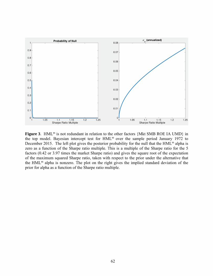
62

Figure 3. HMLm is not redundant in relation to the other factors {Mkt SMB ROE IA UMD} in the top model. Bayesian intercept test for HMLm over the sample period January 1972 to December 2015. The left plot gives the posterior probability for the null that the HMLm alpha is zero as a function of the Sharpe ratio multiple. This is a multiple of the Sharpe ratio for the 5 factors (0.42 or 3.97 times the market Sharpe ratio) and gives the square root of the expectation of the maximum squared Sharpe ratio, taken with respect to the prior under the alternative that the HMLm alpha is nonzero. The plot on the right gives the implied standard deviation of the prior for alpha as a function of the Sharpe ratio multiple.

 

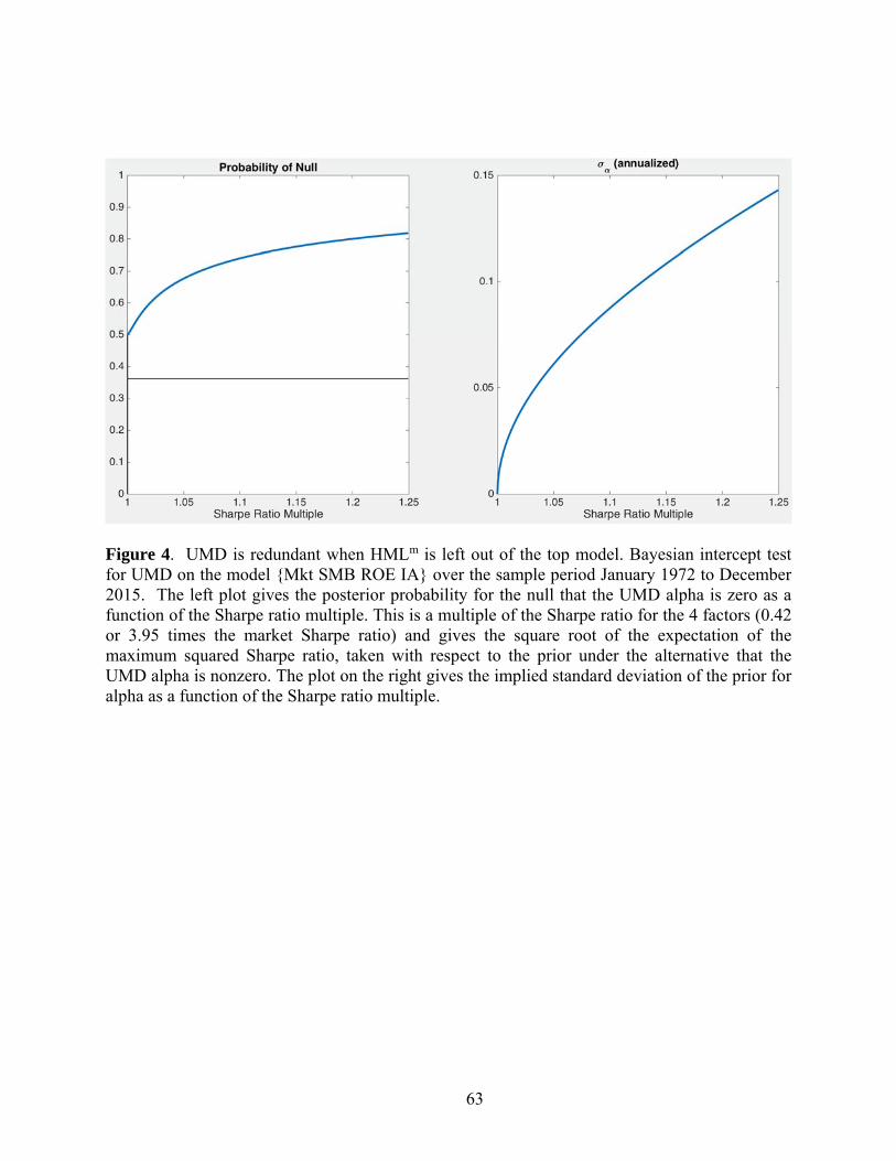
63

Figure 4. UMD is redundant when HMLm is left out of the top model. Bayesian intercept test for UMD on the model {Mkt SMB ROE IA} over the sample period January 1972 to December 2015. The left plot gives the posterior probability for the null that the UMD alpha is zero as a function of the Sharpe ratio multiple. This is a multiple of the Sharpe ratio for the 4 factors (0.42 or 3.95 times the market Sharpe ratio) and gives the square root of the expectation of the maximum squared Sharpe ratio, taken with respect to the prior under the alternative that the UMD alpha is nonzero. The plot on the right gives the implied standard deviation of the prior for alpha as a function of the Sharpe ratio multiple.

 

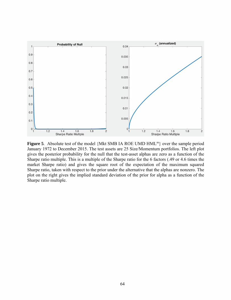
64

Figure 5. Absolute test of the model {Mkt SMB IA ROE UMD HMLm} over the sample period January 1972 to December 2015. The test assets are 25 Size/Momentum portfolios. The left plot gives the posterior probability for the null that the test-asset alphas are zero as a function of the Sharpe ratio multiple. This is a multiple of the Sharpe ratio for the 6 factors (.49 or 4.6 times the market Sharpe ratio) and gives the square root of the expectation of the maximum squared Sharpe ratio, taken with respect to the prior under the alternative that the alphas are nonzero. The plot on the right gives the implied standard deviation of the prior for alpha as a function of the Sharpe ratio multiple.

 

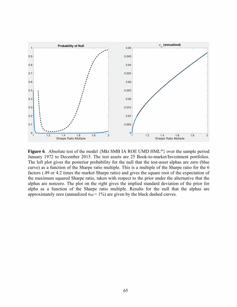
65

Figure 6. Absolute test of the model {Mkt SMB IA ROE UMD HMLm} over the sample period January 1972 to December 2015. The test assets are 25 Book-to-market/Investment portfolios. The left plot gives the posterior probability for the null that the test-asset alphas are zero (blue curve) as a function of the Sharpe ratio multiple. This is a multiple of the Sharpe ratio for the 6 factors (.49 or 4.2 times the market Sharpe ratio) and gives the square root of the expectation of the maximum squared Sharpe ratio, taken with respect to the prior under the alternative that the alphas are nonzero. The plot on the right gives the implied standard deviation of the prior for alpha as a function of the Sharpe ratio multiple. Results for the null that the alphas are approximately zero (annualized σα0

= 1%) are given by the black dashed curves.

 

 

66

Table I

Prior Sensitivity for the Model Probabilities with 10 factors

The table explores sensitivity to the prior of posterior model probabilities (in percent) for the 7 models with highest probability (ranked at the end of the sample) when the prior multiple is set to be 1.5 times the sample market Sharpe ratio, Sh(Mkt). Four prior multiples are considered: 1.25, 1.5, 2.0 and 3.0. The sample period is January 1972 to December 2015. Models are based on 10 prominent factors: the Fama and French (2015) factors (Mkt, HML, SMB, CMA, RMW), the HXZ (2015a) factors (Mkt, ME, ROE, IA), the Asness and Frazzini (2013) value factor HMLm and the Carhart (1997) momentum factor UMD. Each model contains at most one factor from the following categories: size (Mkt or ME), value (HML or HMLm), investment (CMA or IA) and profitability (RMW or ROE). The prior is set so that Shmax = prior multiple x Sh(Mkt), where Shmax is the square root of the expectation of the maximum squared Sharpe ratio with six factors included, taken with respect to the prior under the alternative that the non-market factor alphas are nonzero. Sh(Mkt) is 0.113 and the sample Sharpe ratio for the top-ranked model is 0.51 or 4.5 times Sh(Mkt).

Model/Prior Multiple 1.25 1.5 2 3 Mkt SMB ROE IA HMLm UMD 24.8 38.5 46.8 50.0 Mkt SMB ROE CMA HMLm UMD 10.5 14.8 16.3 16.2 Mkt ME ROE IA HMLm UMD 11.0 13.7 13.4 12.2 Mkt ROE IA HMLm UMD 17.5 13.7 9.3 8.0 Mkt ROE CMA HMLm UMD 7.9 6.0 4.0 3.3 Mkt ME ROE CMA HMLm UMD 4.8 5.4 4.8 4.1 Mkt SMB ROE HMLm UMD 1.5 2.3 3.0 4.1

 

67

Table II

Prior Sensitivity for the Categorical Model Probabilities with 10 factors

The table explores sensitivity to the prior of posterior model probabilities (in percent) for the 7 categorical models with highest probability (ranked at the end of the sample) when the prior multiple is set to be 1.5 times the sample market Sharpe ratio, Sh(Mkt). Four prior multiples are considered: 1.25, 1.5, 2.0 and 3.0. The sample period is January 1972 to December 2015. The factors consist of the market (Mkt) and momentum (UMD), along with the categorical factors (2 versions of each) size, value (VAL), investment (INV) and profitability (PROF). The prior is set so that Shmax = prior multiple x Sh(Mkt), where Shmax is the square root of the expectation of the maximum squared Sharpe ratio with six factors included, taken with respect to the prior under the alternative that the non-market factor alphas are nonzero. Sh(Mkt) is 0.113 and the sample Sharpe ratio for the top-ranked model is 0.51 or 4.5 times Sh(Mkt).

Model/Prior Multiple 1.25 1.5 2 3

Mkt SIZE PROF INV VAL MOM 53.0 72.8 81.4 82.4 Mkt PROF INV VAL MOM 27.2 20.0 13.3 11.3 Mkt PROF SIZE VAL MOM 2.2 3.1 3.8 5.1 Mkt PROF SIZE VAL INV 8.7 2.4 0.7 0.3 Mkt PROF VAL MOM 1.2 0.9 0.7 0.8 Mkt SIZE PROF INV 3.1 0.5 0.1 0.0 Mkt PROF INV VAL 2.3 0.2 0.0 0.0

 

68

Table III

Categorical Factor Shares in the 10-factor Analysis

The table explores sensitivity to the prior of the probability share (in percent) for each categorical factor in the 10-factor analysis under different prior specifications. The share refers to the cumulative posterior probability for the given version of the categorical factor divided by the sum of cumulative probabilities for both versions of the factor. For each categorical factor, the version with the highest probability is shown. The remaining PROF, INV, SIZE and VAL posterior probability goes to RMW, CMA, ME and HML, respectively. The sample period is January 1972 to December 2015. The prior is set so that Shmax = prior multiple x Sh(Mkt), where Shmax is the square root of the expectation of the maximum squared Sharpe ratio with six factors included, taken with respect to the prior under the alternative that the non-market factor alphas are nonzero.

Factor/Prior Multiple 1.25 1.5 2 3

ROE 96.1 99.4 99.9 100 IA 71.3 72.0 73.6 74.9

SMB 68.6 73.4 77.6 80.2 HMLm 94.9 99.5 99.9 100

 

69

Table IV

Intercepts for each Factor in the Six-Factor Model on the other Factors

The table presents annualized alphas from regressions of each factor on the other five factors in the model {Mkt SMB ROE IA UMD HMLm}. This model has the highest posterior probability in the 10-factor analysis. The sample period is from January 1972 to December 2013. T-statistics are reported in parentheses.

 

Factor SMB ROE IA UMD HMLm

Alpha (t-statistic)

4.70 (3.01)

6.51 (5.90)

1.17 (1.51)

6.44 (4.05)

5.59 (5.05)

 

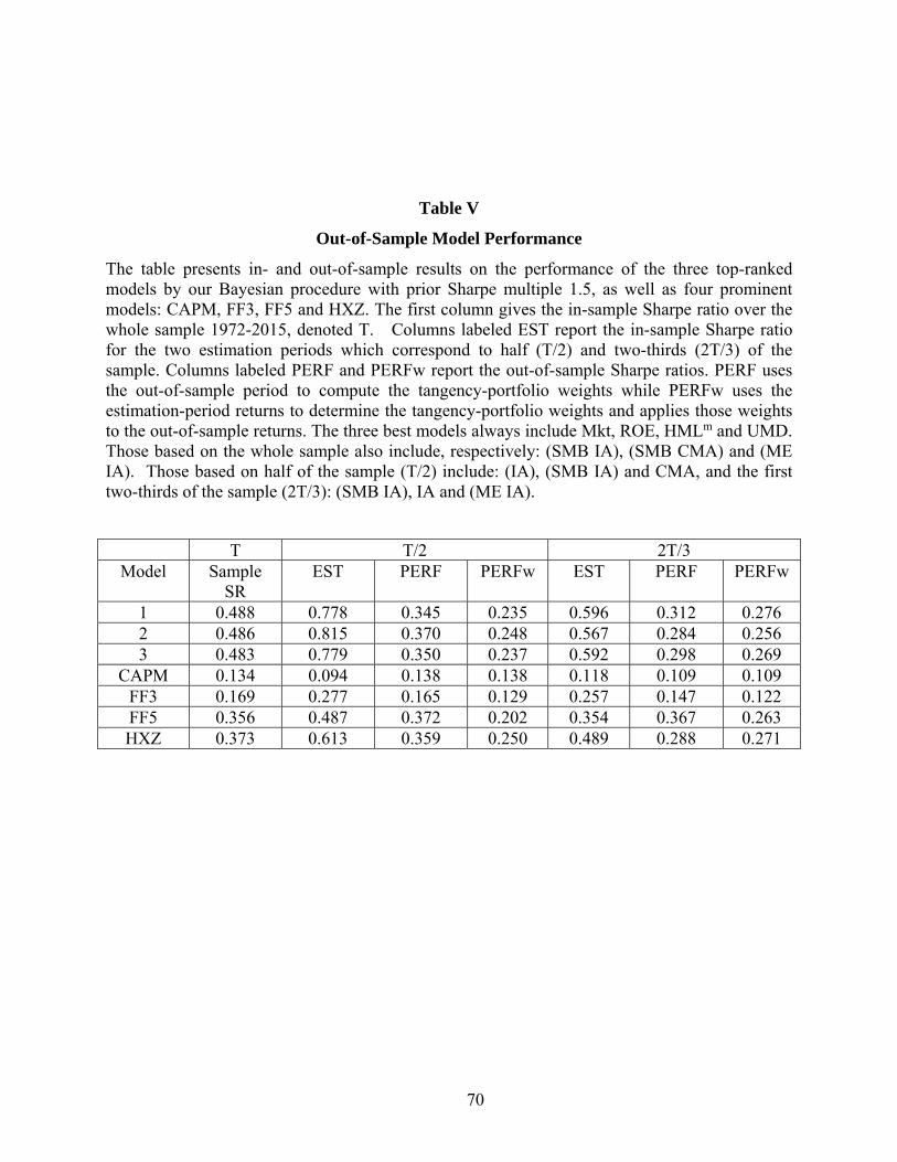
70

Table V

Out-of-Sample Model Performance

The table presents in- and out-of-sample results on the performance of the three top-ranked models by our Bayesian procedure with prior Sharpe multiple 1.5, as well as four prominent models: CAPM, FF3, FF5 and HXZ. The first column gives the in-sample Sharpe ratio over the whole sample 1972-2015, denoted T. Columns labeled EST report the in-sample Sharpe ratio for the two estimation periods which correspond to half (T/2) and two-thirds (2T/3) of the sample. Columns labeled PERF and PERFw report the out-of-sample Sharpe ratios. PERF uses the out-of-sample period to compute the tangency-portfolio weights while PERFw uses the estimation-period returns to determine the tangency-portfolio weights and applies those weights to the out-of-sample returns. The three best models always include Mkt, ROE, HMLm and UMD. Those based on the whole sample also include, respectively: (SMB IA), (SMB CMA) and (ME IA). Those based on half of the sample (T/2) include: (IA), (SMB IA) and CMA, and the first two-thirds of the sample (2T/3): (SMB IA), IA and (ME IA).

T T/2 2T/3 Model Sample

SR EST PERF PERFw EST PERF PERFw

1 0.488 0.778 0.345 0.235 0.596 0.312 0.276 2 0.486 0.815 0.370 0.248 0.567 0.284 0.256 3 0.483 0.779 0.350 0.237 0.592 0.298 0.269

CAPM 0.134 0.094 0.138 0.138 0.118 0.109 0.109 FF3 0.169 0.277 0.165 0.129 0.257 0.147 0.122 FF5 0.356 0.487 0.372 0.202 0.354 0.367 0.263 HXZ 0.373 0.613 0.359 0.250 0.489 0.288 0.271

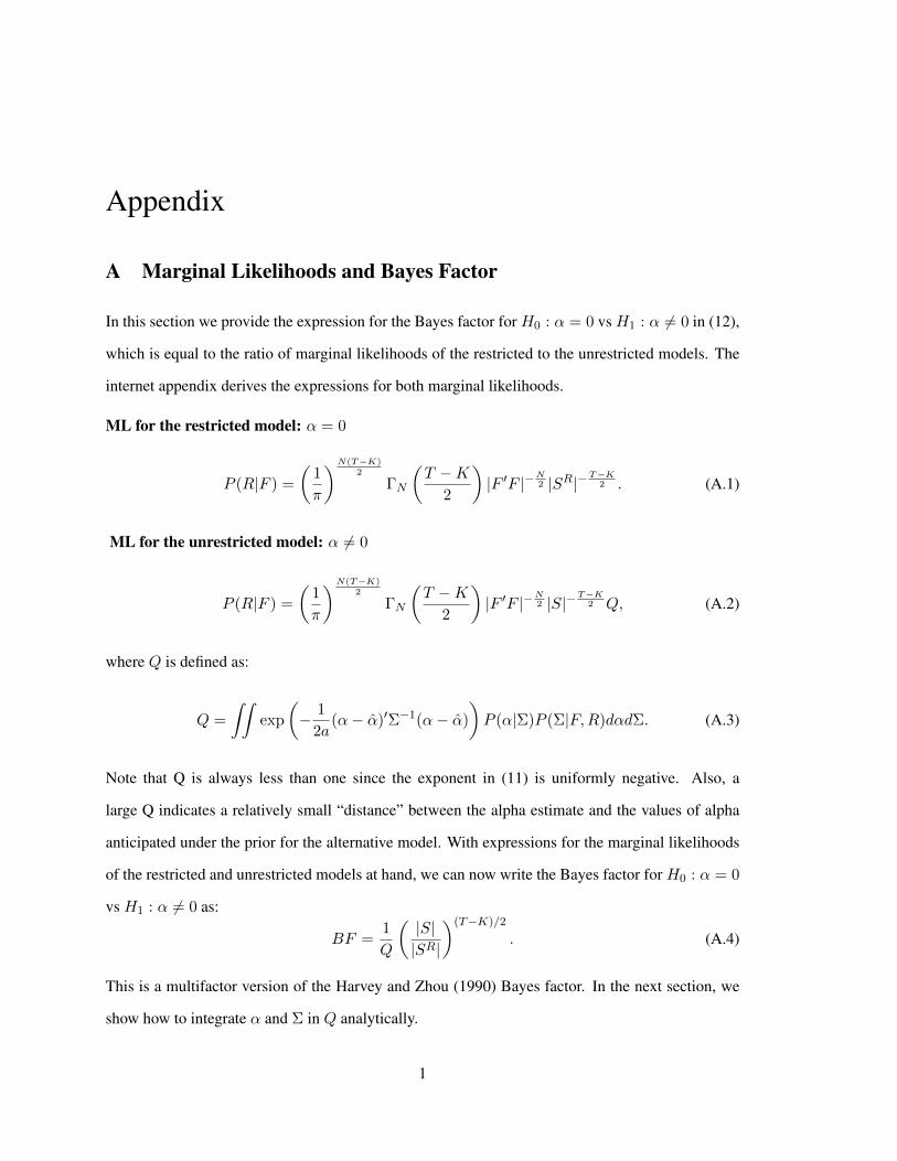
Appendix

A Marginal Likelihoods and Bayes Factor

In this section we provide the expression for the Bayes factor for H0 : α = 0 vs H1 : α 6= 0 in (12),

which is equal to the ratio of marginal likelihoods of the restricted to the unrestricted models. The

internet appendix derives the expressions for both marginal likelihoods.

ML for the restricted model: α = 0

P (R|F ) =

(1

π

)N(T−K)2

ΓN

(T −K

2

)|F ′F |−

N2 |SR|−

T−K2 . (A.1)

ML for the unrestricted model: α 6= 0

P (R|F ) =

(1

π

)N(T−K)2

ΓN

(T −K

2

)|F ′F |−

N2 |S|−

T−K2 Q, (A.2)

where Q is defined as:

Q =

∫∫exp

(− 1

2a(α− α)′Σ−1(α− α)

)P (α|Σ)P (Σ|F,R)dαdΣ. (A.3)

Note that Q is always less than one since the exponent in (11) is uniformly negative. Also, a

large Q indicates a relatively small “distance” between the alpha estimate and the values of alpha

anticipated under the prior for the alternative model. With expressions for the marginal likelihoods

of the restricted and unrestricted models at hand, we can now write the Bayes factor for H0 : α = 0

vs H1 : α 6= 0 as:

BF =1

Q

(|S||SR|

)(T−K)/2

. (A.4)

This is a multifactor version of the Harvey and Zhou (1990) Bayes factor. In the next section, we

show how to integrate α and Σ in Q analytically.

1

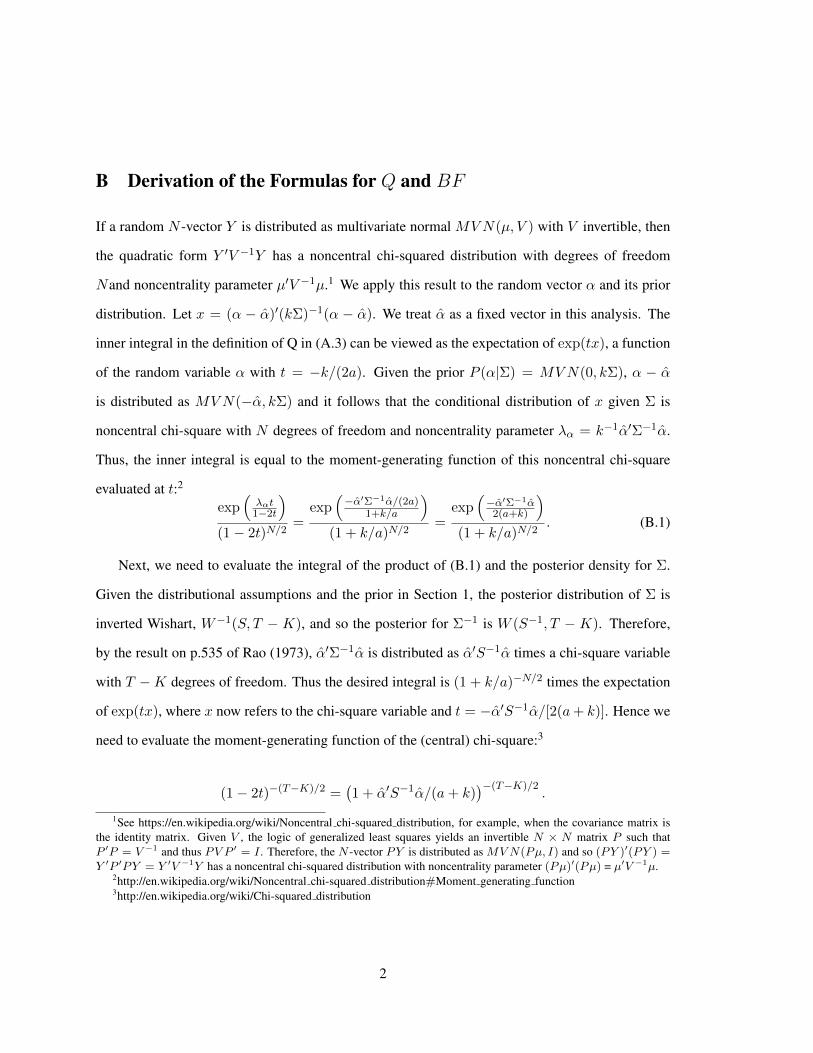
B Derivation of the Formulas for Q and BF

If a random N -vector Y is distributed as multivariate normal MVN(µ, V ) with V invertible, then

the quadratic form Y ′V −1Y has a noncentral chi-squared distribution with degrees of freedom

Nand noncentrality parameter µ′V −1µ.1 We apply this result to the random vector α and its prior

distribution. Let x = (α − α)′(kΣ)−1(α − α). We treat α as a fixed vector in this analysis. The

inner integral in the definition of Q in (A.3) can be viewed as the expectation of exp(tx), a function

of the random variable α with t = −k/(2a). Given the prior P (α|Σ) = MVN(0, kΣ), α − α

is distributed as MVN(−α, kΣ) and it follows that the conditional distribution of x given Σ is

noncentral chi-square with N degrees of freedom and noncentrality parameter λα = k−1α′Σ−1α.

Thus, the inner integral is equal to the moment-generating function of this noncentral chi-square

evaluated at t:2

exp(λαt

1−2t

)(1− 2t)N/2

=exp

(−α′Σ−1α/(2a)

1+k/a

)(1 + k/a)N/2

=exp

(−α′Σ−1α

2(a+k)

)(1 + k/a)N/2

. (B.1)

Next, we need to evaluate the integral of the product of (B.1) and the posterior density for Σ.

Given the distributional assumptions and the prior in Section 1, the posterior distribution of Σ is

inverted Wishart, W−1(S, T − K), and so the posterior for Σ−1 is W (S−1, T − K). Therefore,

by the result on p.535 of Rao (1973), α′Σ−1α is distributed as α′S−1α times a chi-square variable

with T −K degrees of freedom. Thus the desired integral is (1 + k/a)−N/2 times the expectation

of exp(tx), where x now refers to the chi-square variable and t = −α′S−1α/[2(a+ k)]. Hence we

need to evaluate the moment-generating function of the (central) chi-square:3

(1− 2t)−(T−K)/2 =(1 + α′S−1α/(a+ k)

)−(T−K)/2.

1See https://en.wikipedia.org/wiki/Noncentral chi-squared distribution, for example, when the covariance matrix isthe identity matrix. Given V , the logic of generalized least squares yields an invertible N × N matrix P such thatP ′P = V −1 and thus PV P ′ = I . Therefore, the N -vector PY is distributed as MVN(Pµ, I) and so (PY )′(PY ) =Y ′P ′PY = Y ′V −1Y has a noncentral chi-squared distribution with noncentrality parameter (Pµ)′(Pµ) = µ′V −1µ.

2http://en.wikipedia.org/wiki/Noncentral chi-squared distribution#Moment generating function3http://en.wikipedia.org/wiki/Chi-squared distribution

2

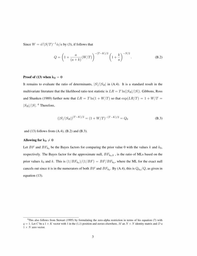
Since W = α′(S/T )−1α/a by (3), if follows that

Q =

(1 +

a

(a+ k)(W/T )

)−(T−K)/2(1 +

k

a

)−N/2. (B.2)

Proof of (13) when k0 = 0

It remains to evaluate the ratio of determinants, |S|/|SR| in (A.4). It is a standard result in the

multivariate literature that the likelihood ratio test statistic is LR = T ln(|SR|/|S|). Gibbons, Ross

and Shanken (1989) further note that LR = T ln(1 + W/T ) so that exp(LR/T ) = 1 + W/T =

|SR|/|S|. 4 Therefore,

(|S|/|SR|)(T−K)/2 = (1 +W/T )−(T−K)/2 = Q0 (B.3)

and (13) follows from (A.4), (B.2) and (B.3).

Allowing for k0 6= 0

Let BF and BFk0 be the Bayes factors for comparing the prior value 0 with the values k and k0,

respectively. The Bayes factor for the approximate null, BFk0,k , is the ratio of MLs based on the

prior values k0 and k. This is (1/BFk0)/(1/BF ) = BF/BFk0 , where the ML for the exact null

cancels out since it is in the numerators of both BF and BFk0 . By (A.4), this is Qk0/Q, as given in

equation (13).

4This also follows from Stewart (1995) by formulating the zero-alpha restriction in terms of his equation (7) withq = 1. Let C be a 1×K vector with 1 in the (1,1) position and zeroes elsewhere, M an N ×N identity matrix and D a1×N zero vector.

3

 

71

C Aggregation over Different Versions of the Categorical Factors

Assume the categorical models consist of up to K factors, KC of which are categorical

factors. In the example of Section IV, with the standard factors Mkt and HML and the

categorical factor Size, K = 3 and KC = 1. There are two versions of the factors, w1 = (Mkt HML

SMB) and w2 = (Mkt HML ME). In general, there are CK2 versions of the K factors, each with

prior probability CK1/ 2 . The K 12  models associated with a given version are assigned uniform

conditional prior probabilities of K 11/ 2 . Let M be a version of a categorical model MC with LC

categorical factors. The number of factor versions that include model M is  CCK L2 (LC slots are

taken), so the fraction of versions that include M is CCC CK L K L2 / 2 1/ 2 . Thus, the total

probability of K 11/ 2  for MC is split evenly between the CL2 versions of that categorical model,

of which M is one. In the example, LC = 0 for {Mkt HML} and LC = 1 for {Mkt ME}. With K =

3, the prior probability for the first model is K 11/ 2 = 1/22 = 1/4, while the probability of the

second is 1/2 ( CL1/ 2 ) of that, or 1/8.

As mentioned earlier, it is essential that the MLs for the various models be based on the

same data. This requires a simple extension of (19). Take the model {Mkt ME), for example. In

the present context, the excluded factors consist of the non-categorical factor HML and the other

version of the categorical Size factor, SMB. We write the ML as the unrestricted ML for ME

given Mkt, times the restricted ML for HML given Mkt and ME, times the restricted ML for

SMB given all three factors in the version w2 = (Mkt HML ME). Thus, the extra ML term at the

end is for the second version of the size factor, which is treated like a test asset conditional on

w2. Similarly, for w1, the extra ML term at the end is for ME given (Mkt HML SMB).

In general, given a K-factor version w, let w* denote the KC alternate versions of the

categorical factors (w2*

would consist of SMB above). Hence there are K + KC factors in all (3 +

1 = 4 in the example). F refers to all of this factor data. For a model M with non-market factors

 

72

f, all contained in w, let f* now denote the factors in w that are excluded from M.31 Let the prior

for the parameters in the regression of w* on (Mkt, f, f*) take the usual form based on (5) and (6),

again independent of the other components. The test-assets r are now regressed on (Mkt, f, f*,

w*), i.e., all the factors, and so the corresponding ML will cancel out in all probability

calculations, as earlier. This term will be ignored going forward. Therefore, the counterpart of

(19) is now

ML(M | w) = MLU(f | Mkt) x MLR(f* | Mkt, f) x MLR(w* | Mkt, f, f*). (C.1)

For each w, the conditional posterior probabilities can then be obtained as in (17). Note that the

ML term corresponding to w* will drop out of these computations that are conditional on w. The

w* term will differ across the various w’s, however, and so will affect the posterior probabilities

for the w’s, as we now see.

Proposition 4. The unconditional (not conditional on w) posterior model probabilities are

obtained as follows. First, calculate ML(M | w) in (C.1) for each version w of the factors and

each model in w. Then calculate the ML for each was:

ML(w) = EM|w{ML(M | w)}. (C.2)

where M|w refers to the uniform prior over the models in w. Next, calculate the unconditional

probability of the data,

P(F) = Ew{ML(w)}, (C.3)

by averaging ML(w) over the uniform prior P(w). The posterior probability for each w is then

P(w | F) = ML(w)P(w)/P(F). (C.4)

Finally, the unconditional posterior probability for M is

P(M | F) = Ew|F{P(M | w, F)}, (C.5)

                                                       31 f* will differ across the different w’s that include the factors f (a w subscript is implicit).

 

73

where P(M | w, F) is the conditional posterior probability for M given factor version w and the

expectation is taken with respect to the versions posterior P(w | F).

Proof. A general principle that we use repeatedly is P(Y) = EX{P(Y|X)}. Also, by definition,

ML(M | w) = P(F | M, w) and ML(w) = P(F | w). In (C.2), M plays the role of X and F the role

of Y, while we condition on w throughout in the “background.” In (C.3), w plays the role of X

and F the role of Y. (C.4) is just Bayes’ theorem. Finally, w plays the role of X and M the role

of Y in (C.5), while we condition on F throughout in the background.

Allowing Each Factor to be Included or Not in the Basic Methodology

This generalization of the basic methodology for a single version of the factors is, with a

few modifications, based on Proposition 4. Now, instead of the “hyperparameter” w denoting a

version of the factors, it refers to the factor that plays the anchor role that Mkt plays in (18), (19)

and (C.1) above. Since the entire analysis is no longer conditioned on Mkt or any other factor,

the density of that first factor must now be modeled. Thus, the counterpart of (C.1) is

ML(M | w) = MLU(w) x MLU(f | w) x MLR(f* | w, f), (C.6)

where MLU(w) is the marginal likelihood for factor w assuming it is normally distributed

independently over time, with unknown mean and variance, both of which have standard diffuse

priors. Now f denotes the factors other than w that are in M, while f* consists of the factors that

are excluded from M. One approach is to let the prior parameter k be specified for each anchor

in such a way that the corresponding Shmax is the same for all anchors and equal to the multiple

of the sample Mkt Sharpe ratio used in the main analysis. See the discussion below (19). This

introduces an “empirical Bayesian” element that is common in other Bayesian asset-pricing

papers. The aggregation of conditional probabilities then proceeds exactly as in (C.2) through

(C.5).