Embed Size (px)
Citation preview
(Combinatorics of)Alignment and Gene
FindingLior Pachter
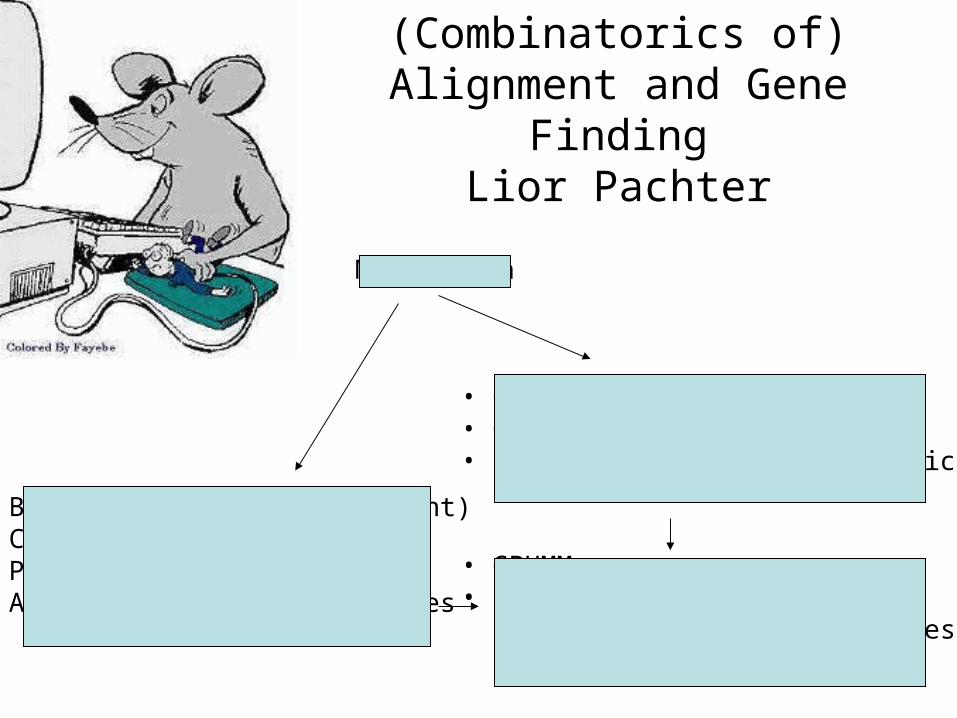
• Basic definitions (alignment)• Combinatorics of alignment• Pair hidden Markov models• Alignment of large sequences
• Gene structure • Generalized HMMs• Intro. to comparative genomics
• GPHMMs• Example: the human and mouse genomes
Motivation
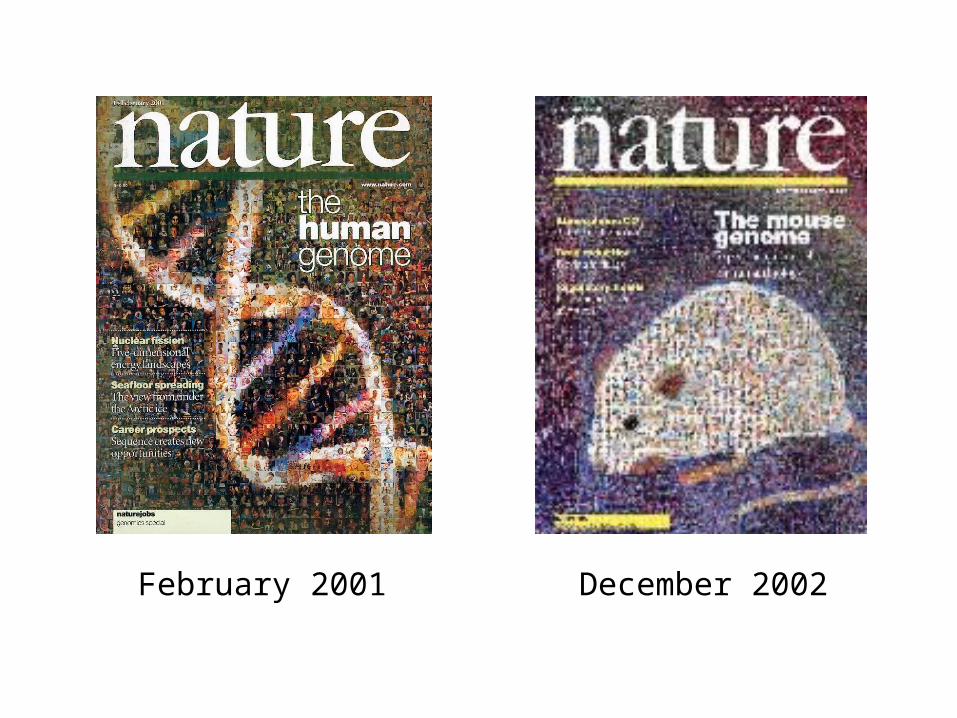
February 2001 December 2002
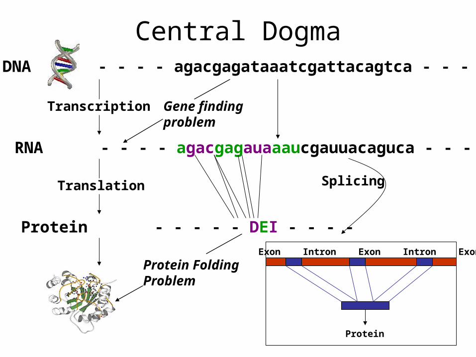
DNA - - - - agacgagataaatcgattacagtca - - - -
Transcription
RNA - - - - agacgagauaaaucgauuacaguca - - - -
Translation
Protein - - - - - DEI - - - -
Protein FoldingProblem
Exon Intron Exon Intron Exon
Protein
Splicing
Central Dogma
Gene findingproblem
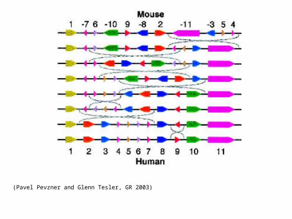
(Pavel Pevzner and Glenn Tesler, GR 2003)
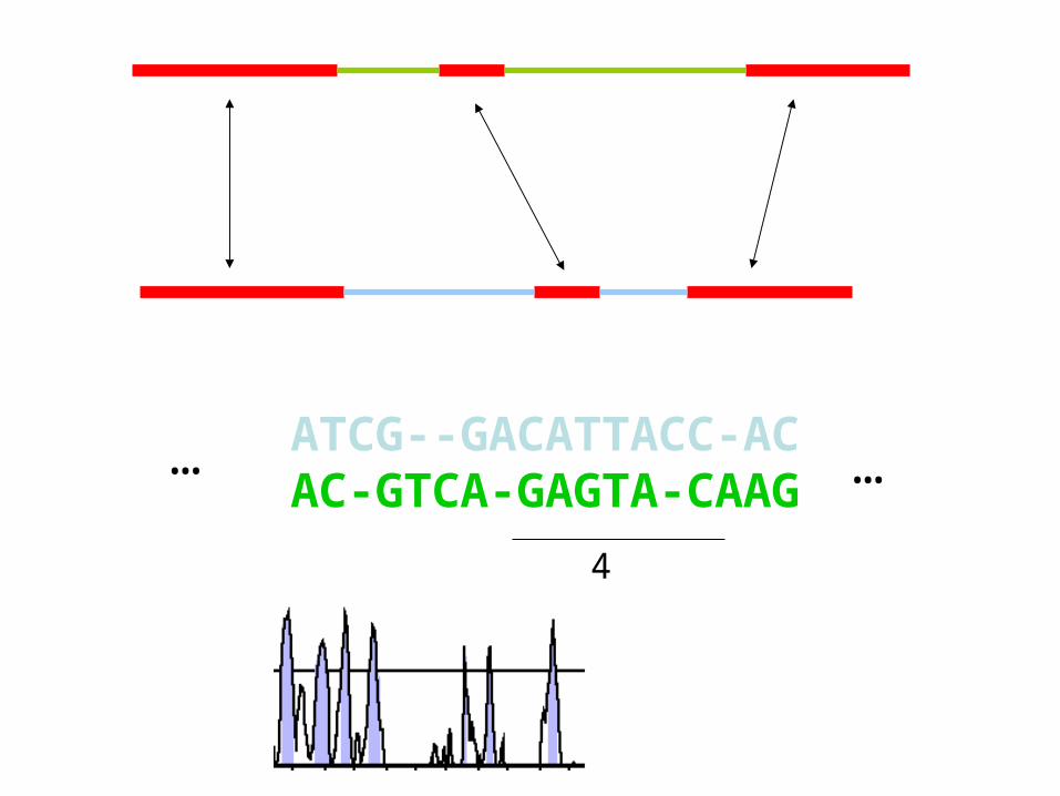
ATCG--GACATTACC-ACAC-GTCA-GAGTA-CAAG
4
… …


Part 1: Alignment
M
X
Y
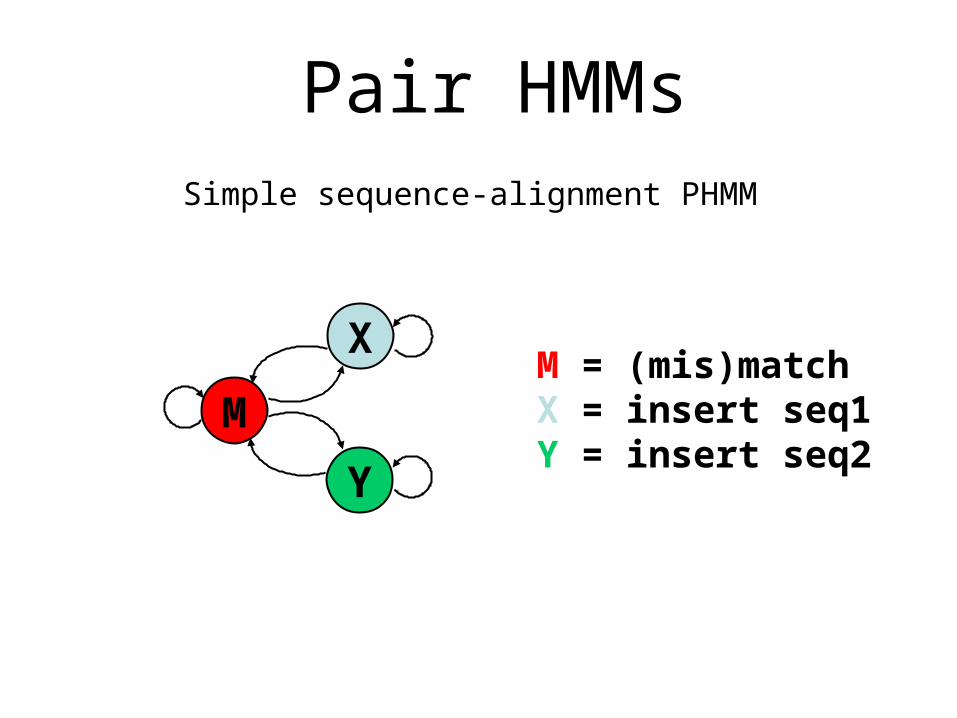
M = (mis)matchX = insert seq1Y = insert seq2
Pair HMMsSimple sequence-alignment PHMM
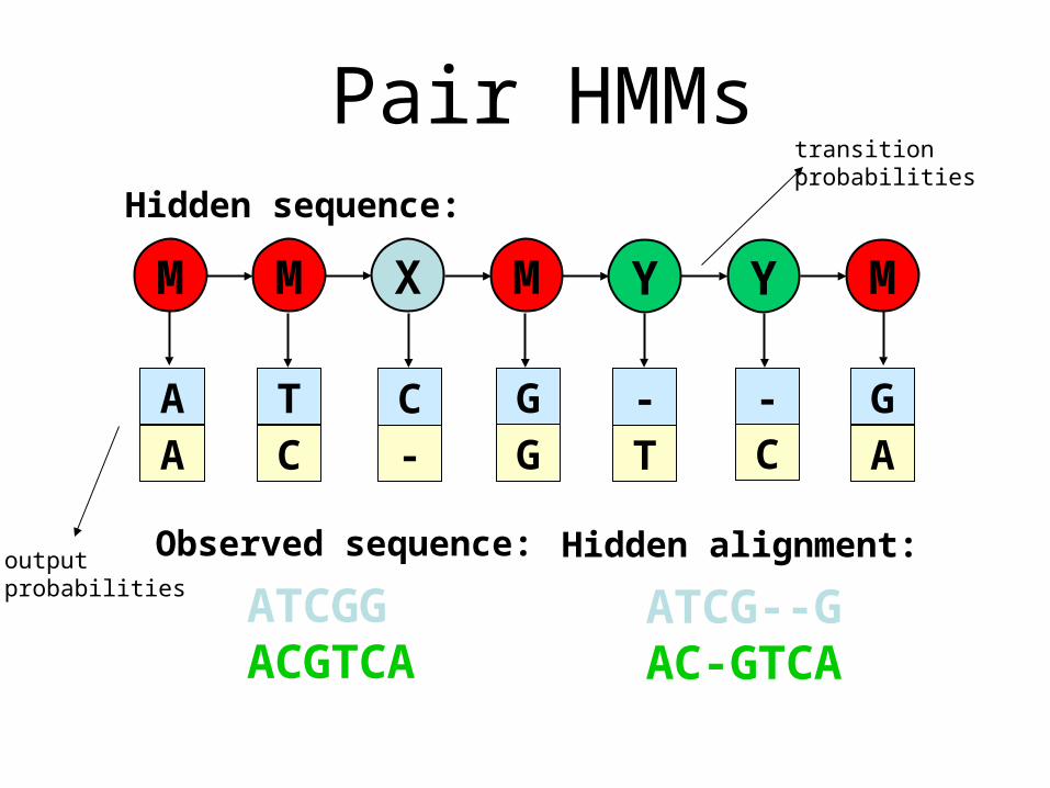
M X YM M Y M
Hidden sequence:
AA
TC
C-
GG
-T
-C
GA
Observed sequence:
ATCGGACGTCA
Hidden alignment:
ATCG--GAC-GTCA
Pair HMMstransitionprobabilities
outputprobabilities
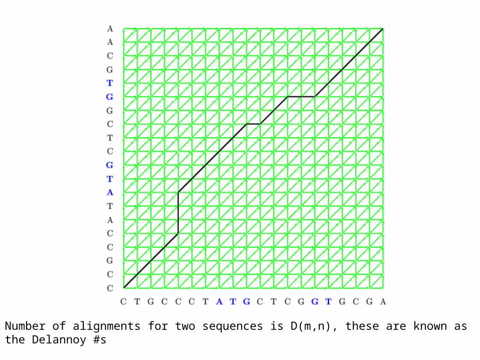
Number of alignments for two sequences is D(m,n), these are known as the Delannoy #s
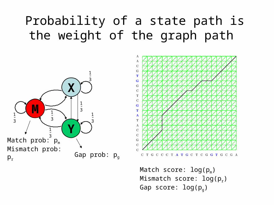
Probability of a state path is the weight of the graph path
M
X
Y1-3
1-3
1-3
1-3
1-3
1-3
Match prob: pm
Mismatch prob: pr
Match score: log(pm)Mismatch score: log(pr)Gap score: log(pg)
Gap prob: pg
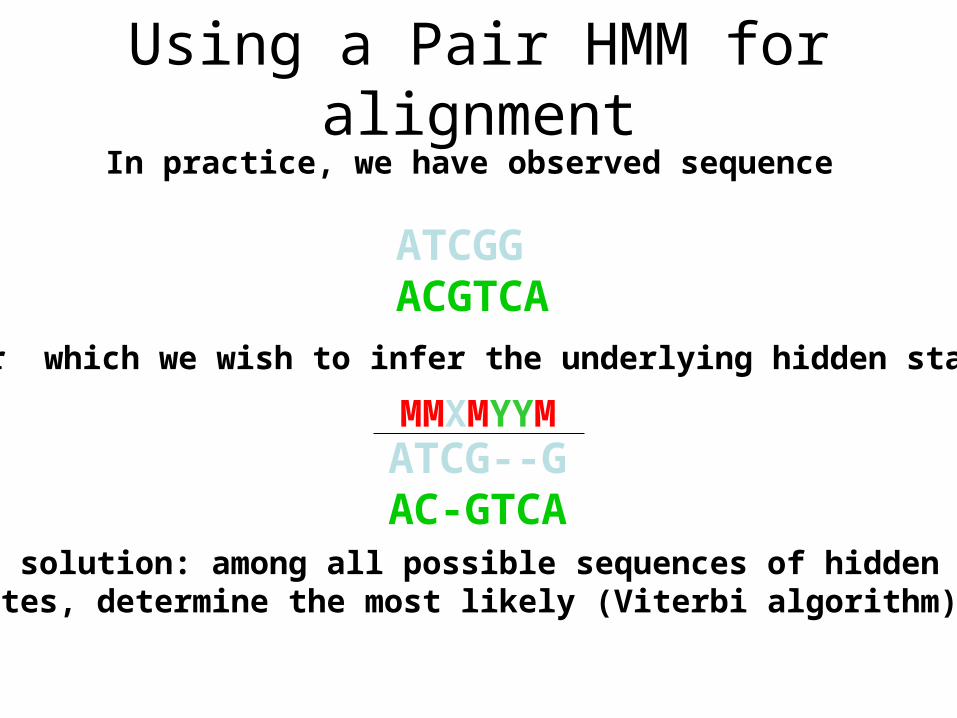
Using a Pair HMM for alignmentIn practice, we have observed sequence
ATCGGACGTCA
for which we wish to infer the underlying hidden states
One solution: among all possible sequences of hiddenstates, determine the most likely (Viterbi algorithm).
ATCG--GAC-GTCA
MMXMYYM
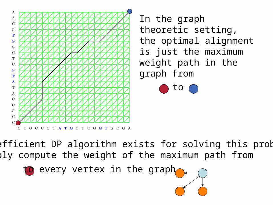
In the graph theoretic setting, the optimal alignment is just the maximum weight path in the graph from
to
An efficient DP algorithm exists for solving this problem:Simply compute the weight of the maximum path from
to every vertex in the graph
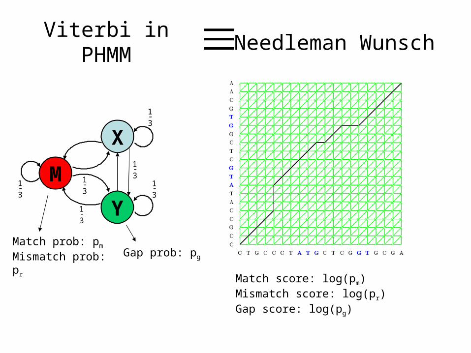
Viterbi in PHMM ≡ Needleman Wunsch
M
X
Y1-3
1-3
1-3
1-3
1-3
1-3
Match prob: pm
Mismatch prob: pr
Match score: log(pm)Mismatch score: log(pr)Gap score: log(pg)
Gap prob: pg
The DP algorithm for alignment has running time O(nm)where n and m are the lengths of the sequences. The memory requirements are also O(nm), however itis possible to reduce this to O(n+m) using divide and conquer.
This approach is not practical for sequence lengthsof much more than 10kb.
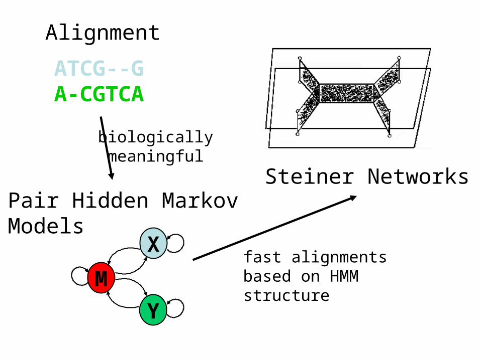
Alignment
Pair Hidden Markov Models
Steiner Networks
ATCG--GA-CGTCA
M
X
Y
biologically meaningful
fast alignmentsbased on HMM structure
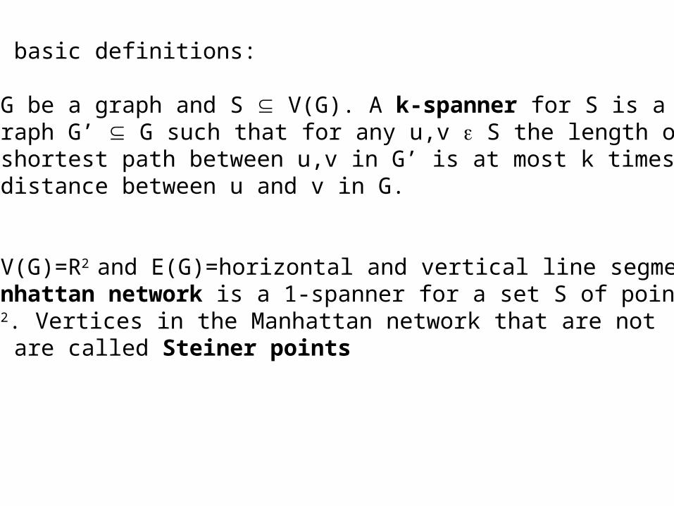
Some basic definitions:
Let G be a graph and S V(G). A k-spanner for S is a subgraph G’ G such that for any u,v S the length of the shortest path between u,v in G’ is at most k timesthe distance between u and v in G.
Let V(G)=R2 and E(G)=horizontal and vertical line segments.A Manhattan network is a 1-spanner for a set S of pointsin R2. Vertices in the Manhattan network that are notin S are called Steiner points
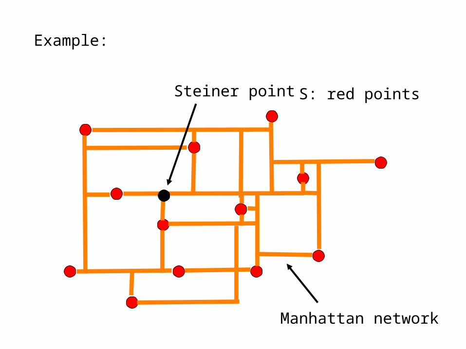
Example:
S: red points
Manhattan network
Steiner point
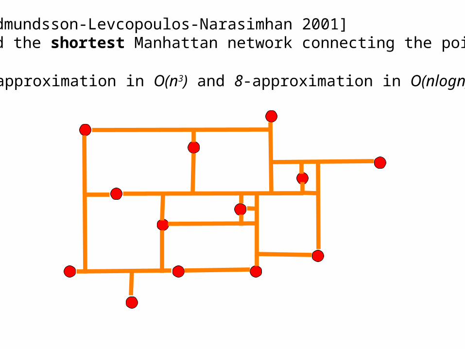
[Gudmundsson-Levcopoulos-Narasimhan 2001] Find the shortest Manhattan network connecting the points
4-approximation in O(n3) and 8-approximation in O(nlogn)
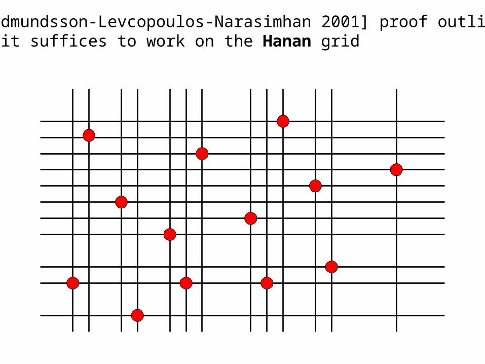
[Gudmundsson-Levcopoulos-Narasimhan 2001] proof outline: 1. it suffices to work on the Hanan grid
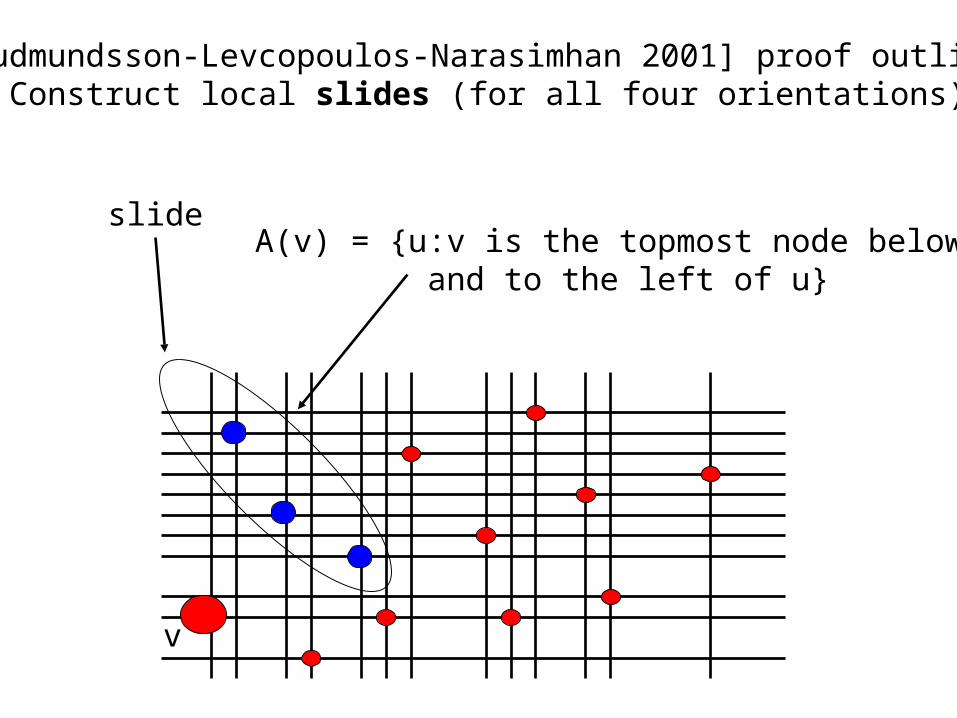
A(v) = {u:v is the topmost node below and to the left of u}
[Gudmundsson-Levcopoulos-Narasimhan 2001] proof outline: 2. Construct local slides (for all four orientations)
v
slide
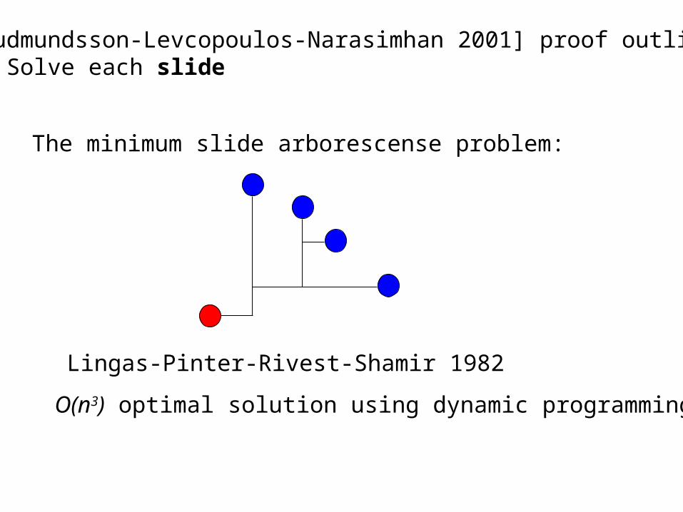
[Gudmundsson-Levcopoulos-Narasimhan 2001] proof outline: 3. Solve each slide
The minimum slide arborescense problem:
Lingas-Pinter-Rivest-Shamir 1982
O(n3) optimal solution using dynamic programming
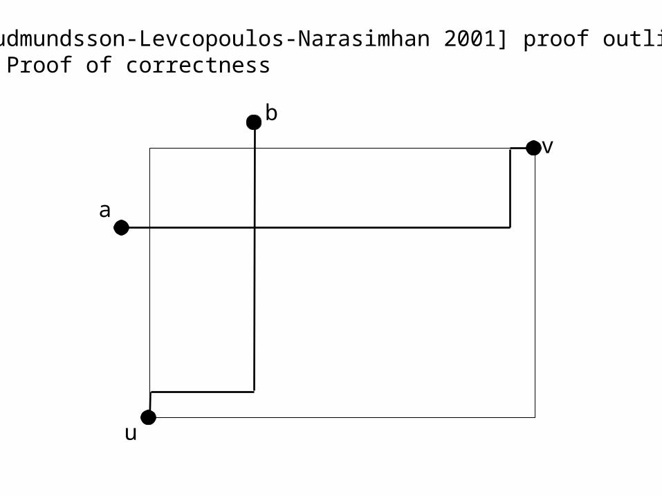
[Gudmundsson-Levcopoulos-Narasimhan 2001] proof outline: 4. Proof of correctness
u
v
b
a
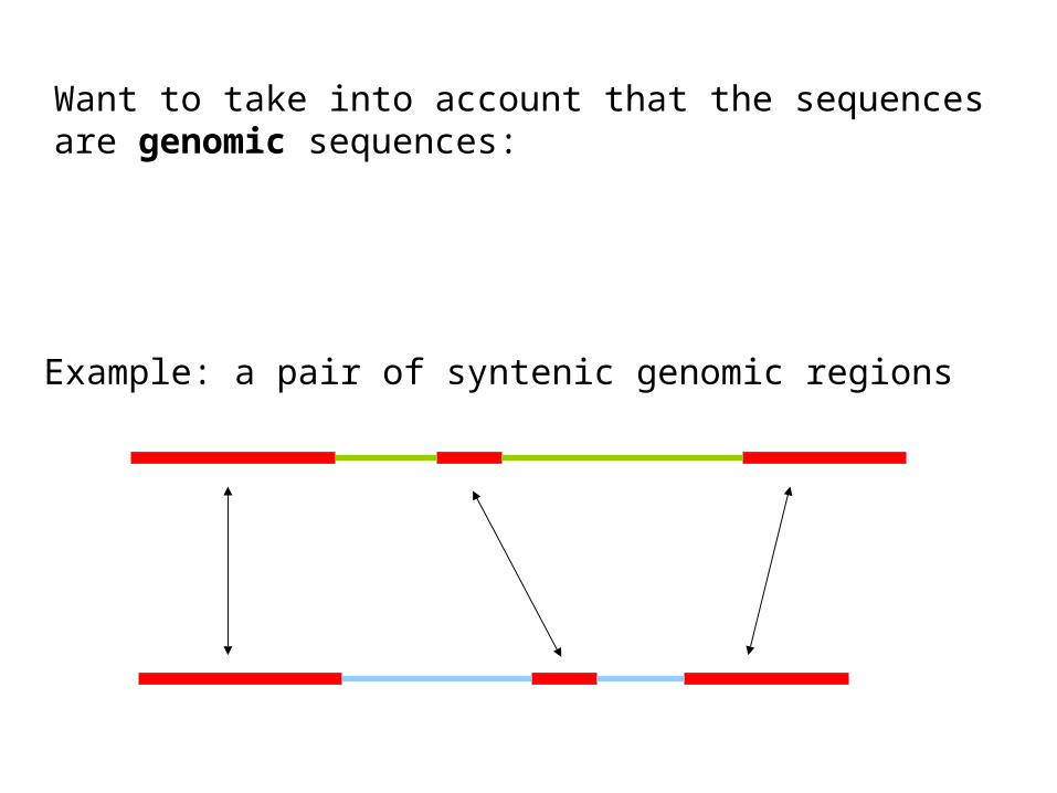
Want to take into account that the sequencesare genomic sequences:
Example: a pair of syntenic genomic regions
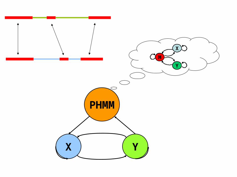
YX
PHMM
M
X
Y
YX
PHMM
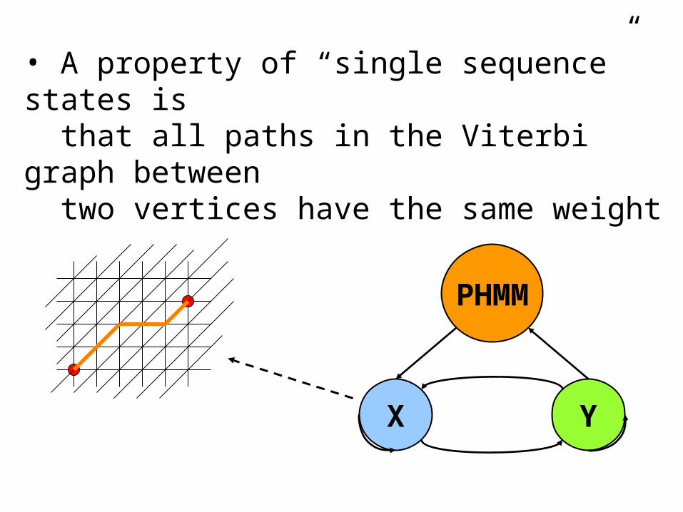
• A property of “single sequence” states is that all paths in the Viterbi graph between two vertices have the same weight
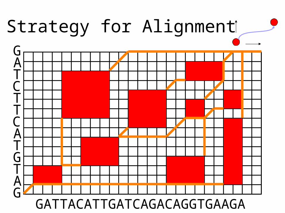
Strategy for Alignment
GATTACATTGATCAGACAGGTGAAGA
GATCTTCATGTAG
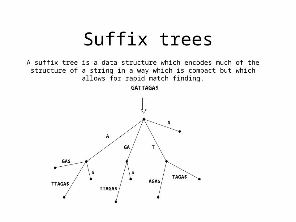
Suffix treesA suffix tree is a data structure which encodes much of the structure of
a string in a way which is compact but which allows for rapid match finding.
GATTAGA$
$
T
TTAGA$
GA
A
GA$
$ $
TTAGA$
TAGA$AGA$
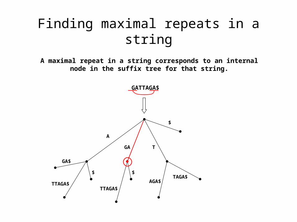
Finding maximal repeats in a string
A maximal repeat in a string corresponds to an internal node in the suffix tree for that string.
GATTAGA$
$
T
TTAGA$
GA
A
GA$
$ $
TTAGA$
TAGA$AGA$
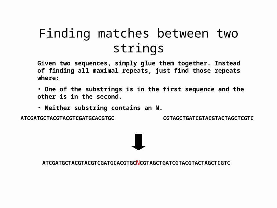
Finding matches between two strings
Given two sequences, simply glue them together. Instead of finding all maximal repeats, just find those repeats where:
• One of the substrings is in the first sequence and the other is in the second.
• Neither substring contains an N.
ATCGATGCTACGTACGTCGATGCACGTGC
CGTAGCTGATCGTACGTACTAGCTCGTC
ATCGATGCTACGTACGTCGATGCACGTGCNCGTAGCTGATCGTACGTACTAGCTCGTC
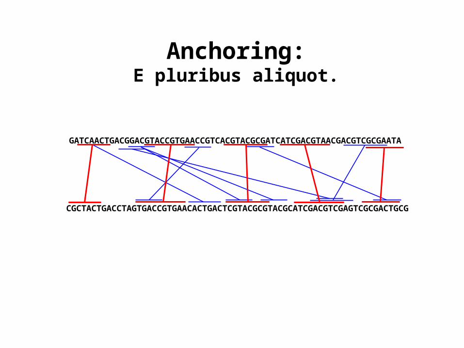
GATCAACTGACGGACGTACCGTGAACCGTCACGTACGCGATCATCGACGTAACGACGTCGCGAATA
CGCTACTGACCTAGTGACCGTGAACACTGACTCGTACGCGTACGCATCGACGTCGAGTCGCGACTGCG
Anchoring:E pluribus aliquot.
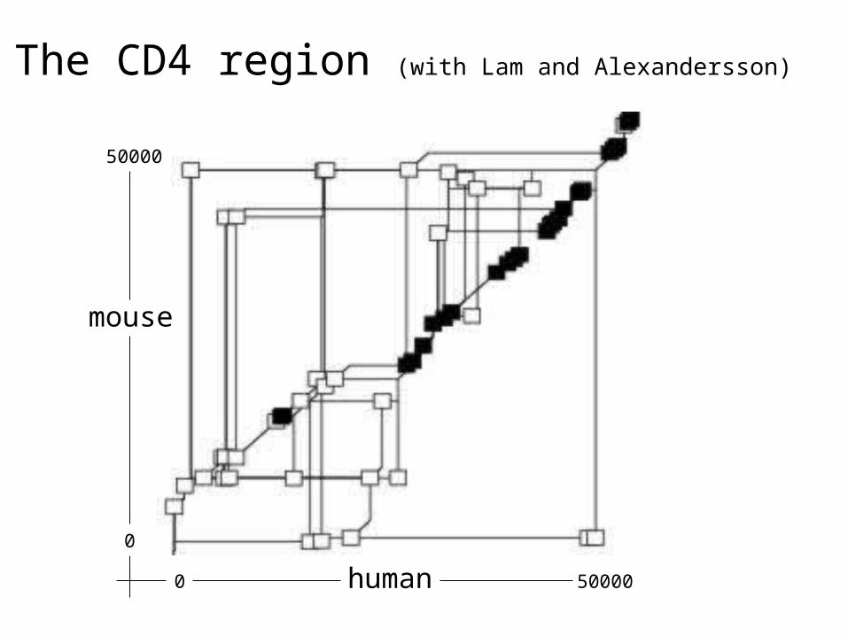
The CD4 region (with Lam and Alexandersson)
human
mouse
50000
50000
0
0
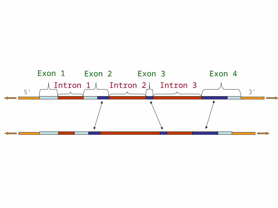
5’ 3’
Exon 1 Exon 2 Exon 3 Exon 4
Intron 1 Intron 2 Intron 3
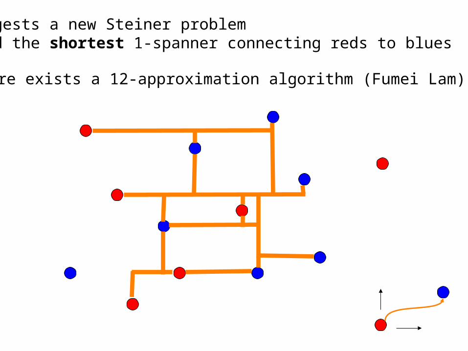
Suggests a new Steiner problemFind the shortest 1-spanner connecting reds to blues
There exists a 12-approximation algorithm (Fumei Lam)
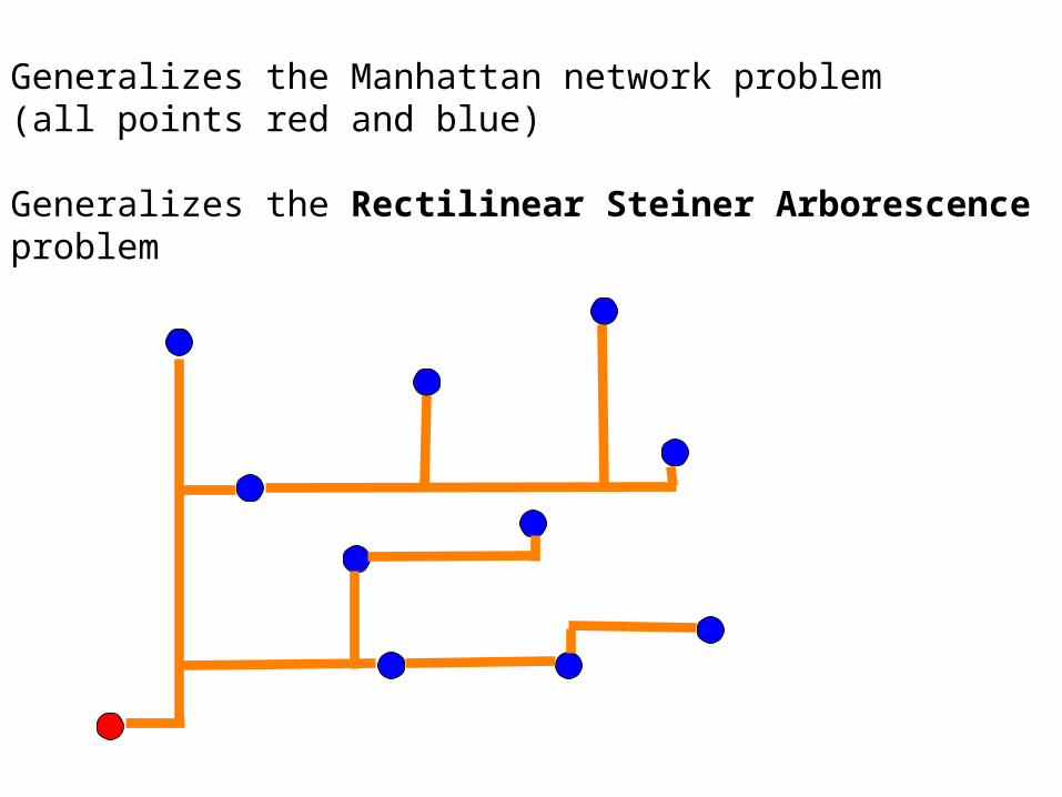
Generalizes the Manhattan network problem (all points red and blue)
Generalizes the Rectilinear Steiner Arborescence problem
1985, Trubin - polynomial time algorithm
History of the Rectilinear Steiner Arborescence Problem
1992, Rao-Sadayappan-Hwang-Shor - error in Trubin
2000, Shi and Su - NP complete!
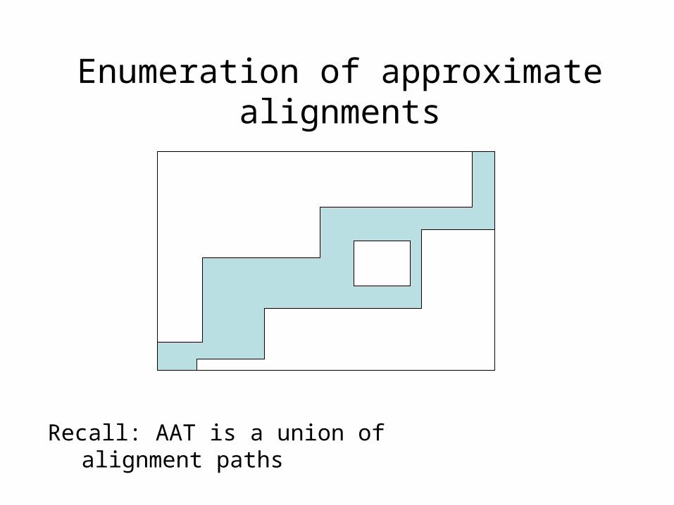
Enumeration of approximate alignments
Recall: AAT is a union of alignment paths
HVC
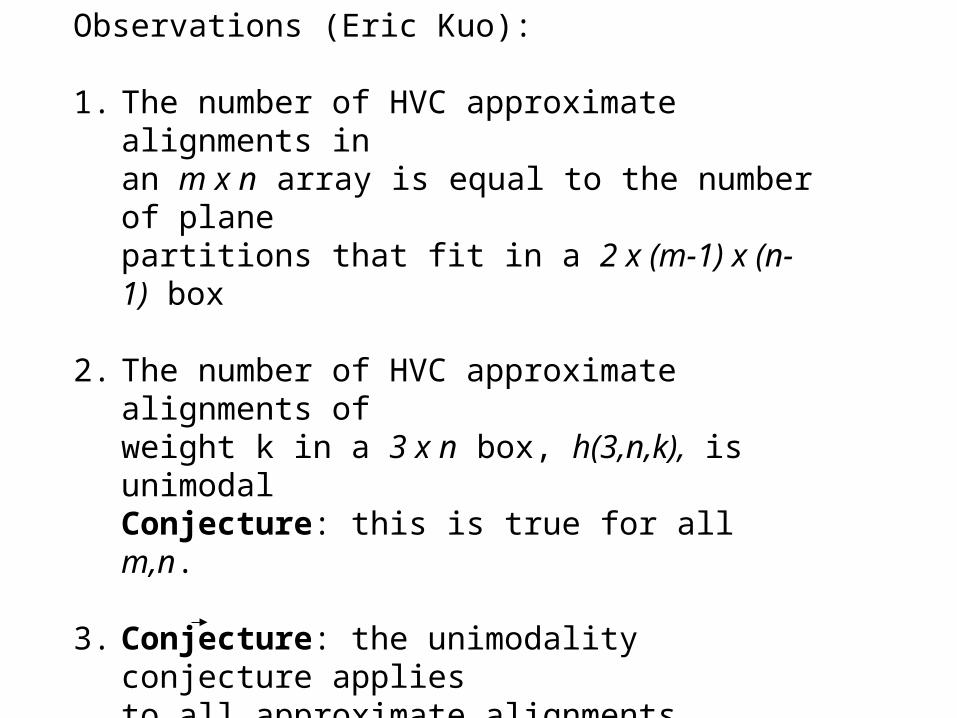
Observations (Eric Kuo):
1. The number of HVC approximate alignments in an m x n array is equal to the number of plane partitions that fit in a 2 x (m-1) x (n-1) box
2. The number of HVC approximate alignments ofweight k in a 3 x n box, h(3,n,k), is unimodalConjecture: this is true for all m,n.
3. Conjecture: the unimodality conjecture appliesto all approximate alignments, G(m,n,k).
4. limm,n ∞ [ G(m+1,n+1)G(m,n)]/[G(m+1,n)G(m,n+1)]
= 1.6479 +
Part 2: Gene Finding (and
alignment)joint work with Simon Cawley and
Marina Alexandersson

DNA - - - - agacgagataaatcgattacagtca - - - -
Transcription
RNA - - - - agacgagauaaaucgauuacaguca - - - -
Translation
Protein - - - - - DEI - - - -
Protein FoldingProblem
Exon Intron Exon Intron Exon
Protein
Splicing
Central Dogma
Gene findingproblem
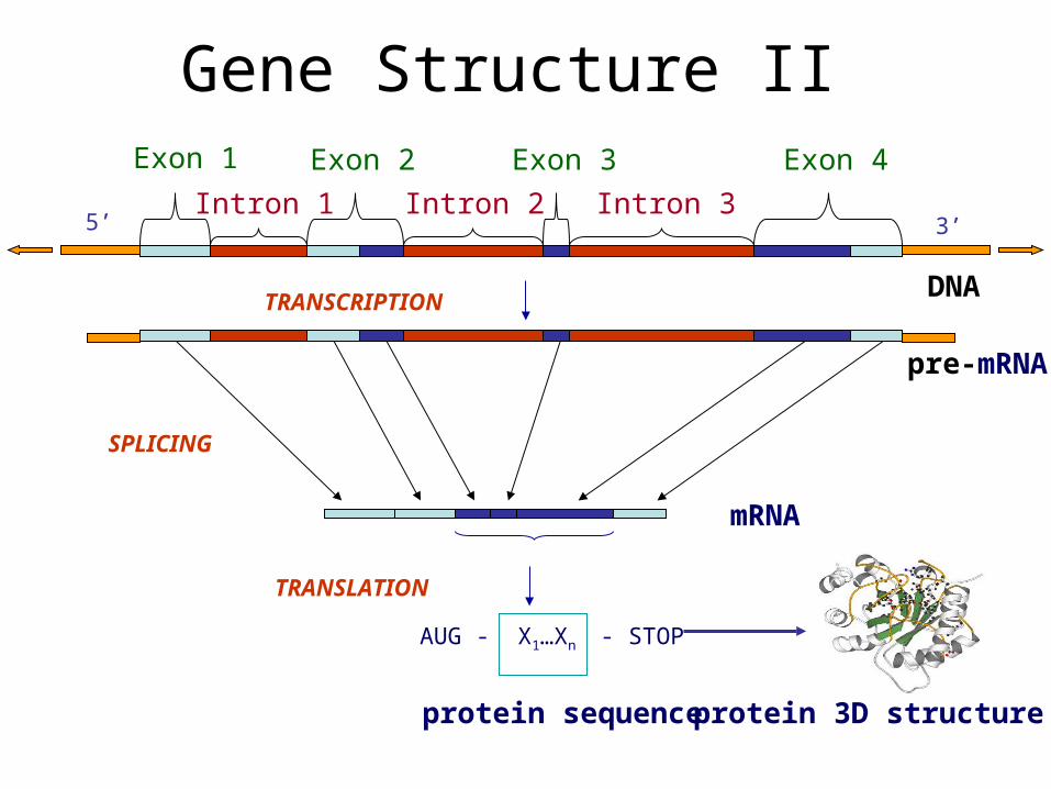
Gene Structure II
AUG - X1…Xn - STOP
SPLICING
TRANSLATION
3’
pre-mRNA
mRNA
protein sequenceprotein 3D structure
Exon 1 Exon 2 Exon 3 Exon 4
Intron 1 Intron 2 Intron 3
DNATRANSCRIPTION
5’
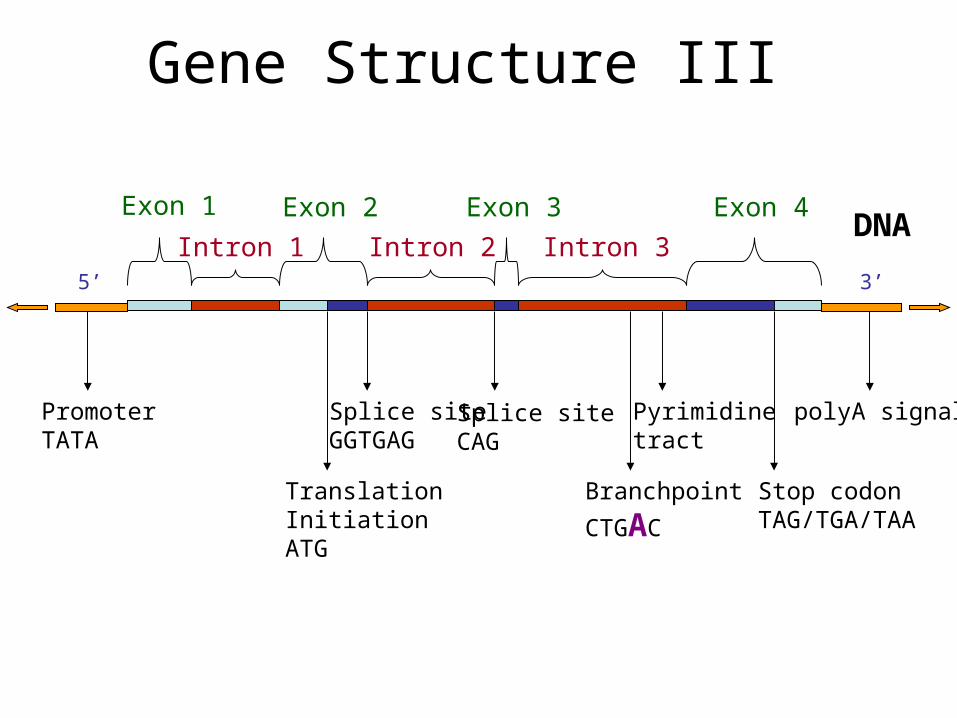
Gene Structure III
5’ 3’
DNAExon 1 Exon 2 Exon 3 Exon 4
Intron 1 Intron 2 Intron 3
polyA signalPyrimidinetract
Branchpoint
CTGAC
Splice siteCAG
Splice siteGGTGAG
TranslationInitiationATG
Stop codonTAG/TGA/TAA
PromoterTATA
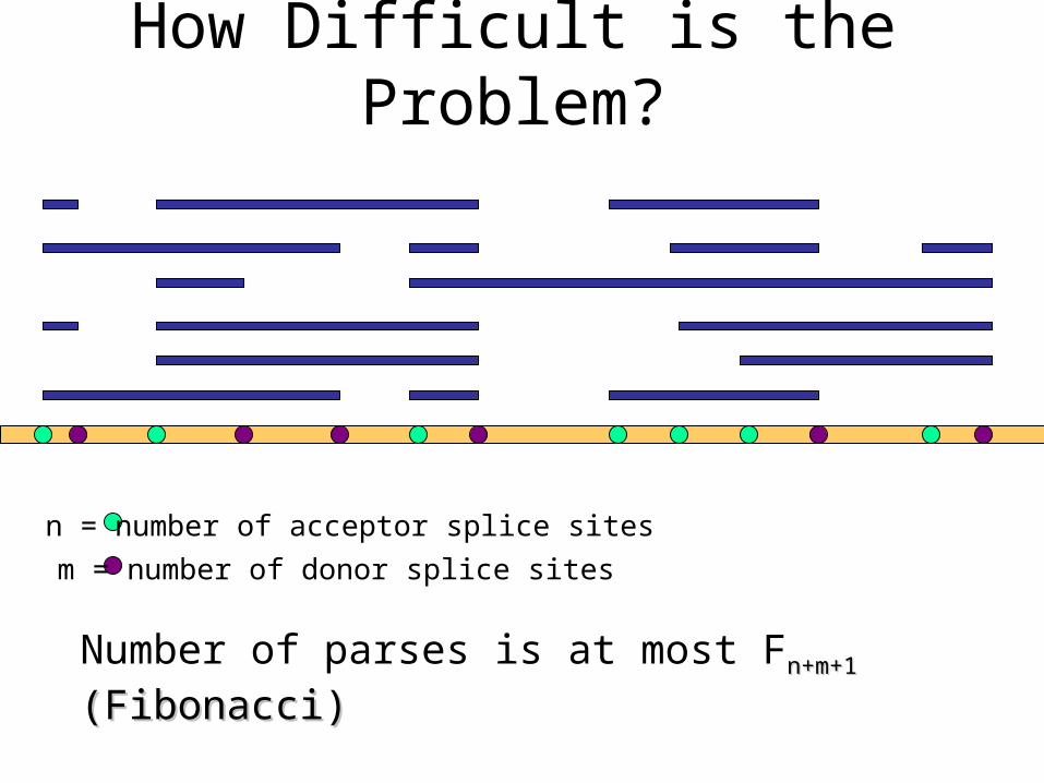
How Difficult is the Problem?
n = number of acceptor splice sites
m = number of donor splice sites
Number of parses is at most Fn+m+1 n+m+1
(Fibonacci)(Fibonacci)
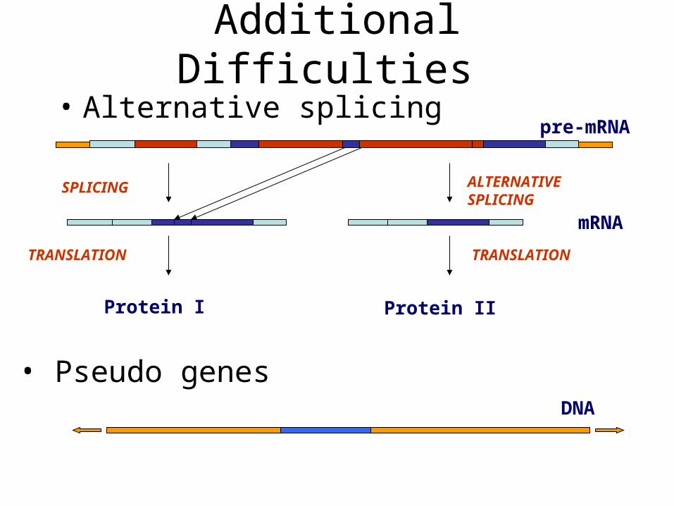
Additional Difficulties
• Alternative splicing
SPLICING
TRANSLATION
pre-mRNA
• Pseudo genes
ALTERNATIVE SPLICING
TRANSLATION
Protein IIProtein I
mRNA
DNA
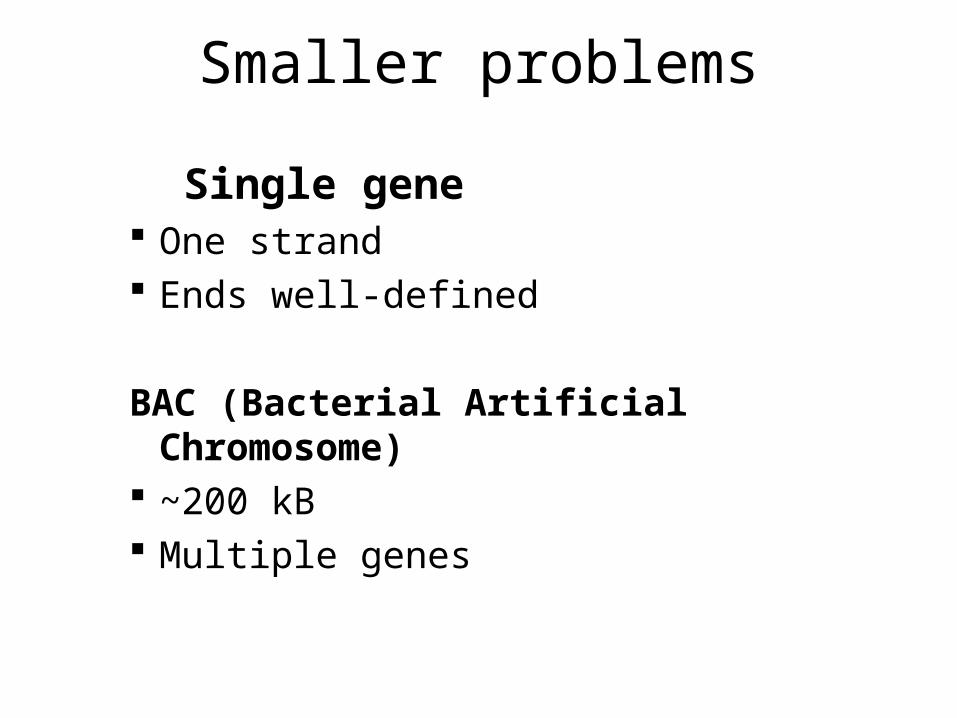
Smaller problems
Single gene One strand Ends well-defined
BAC (Bacterial Artificial Chromosome) ~200 kB Multiple genes
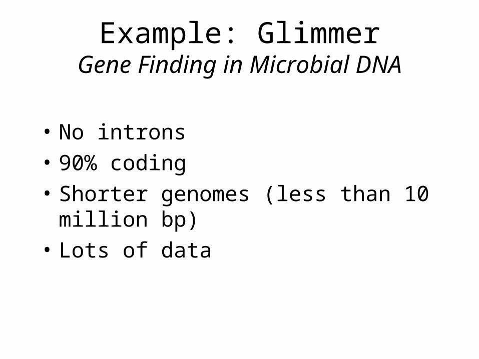
Example: GlimmerGene Finding in Microbial DNA
• No introns
• 90% coding
• Shorter genomes (less than 10 million bp)
• Lots of data
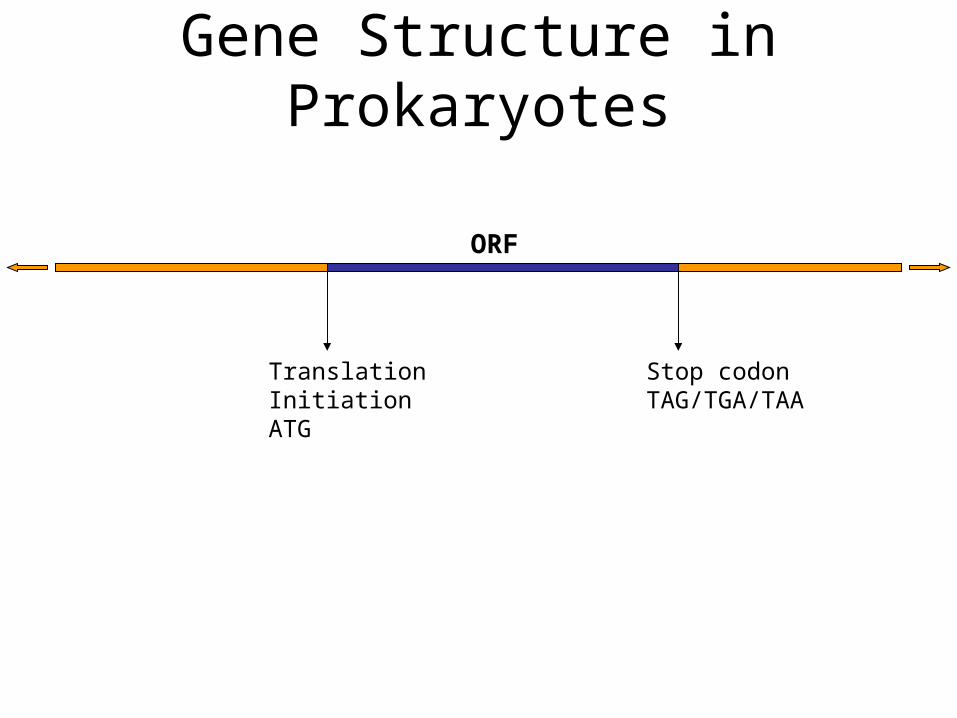
TranslationInitiationATG
Stop codonTAG/TGA/TAA
ORF
Gene Structure in Prokaryotes
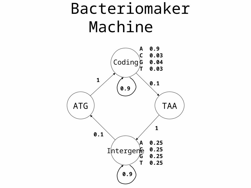
BacteriomakerMachine
Intergene
ATG TAA
Coding
A 0.25C 0.25G 0.25T 0.25
A 0.9C 0.03G 0.04T 0.03
1
1
0.9
0.1
0.1
0.9
Example: GenscanGene Finding in Human DNA
• Introns
• 1.2% coding
• Large genome (3.2 billion bp)
• Alternative splicing
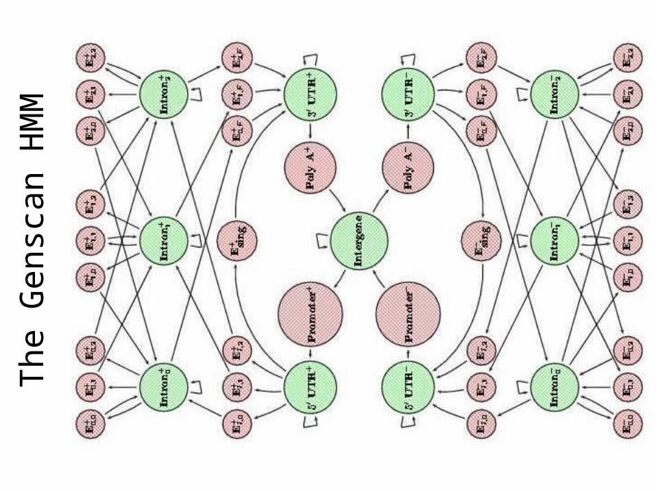
The
Gen
scan
HM
M
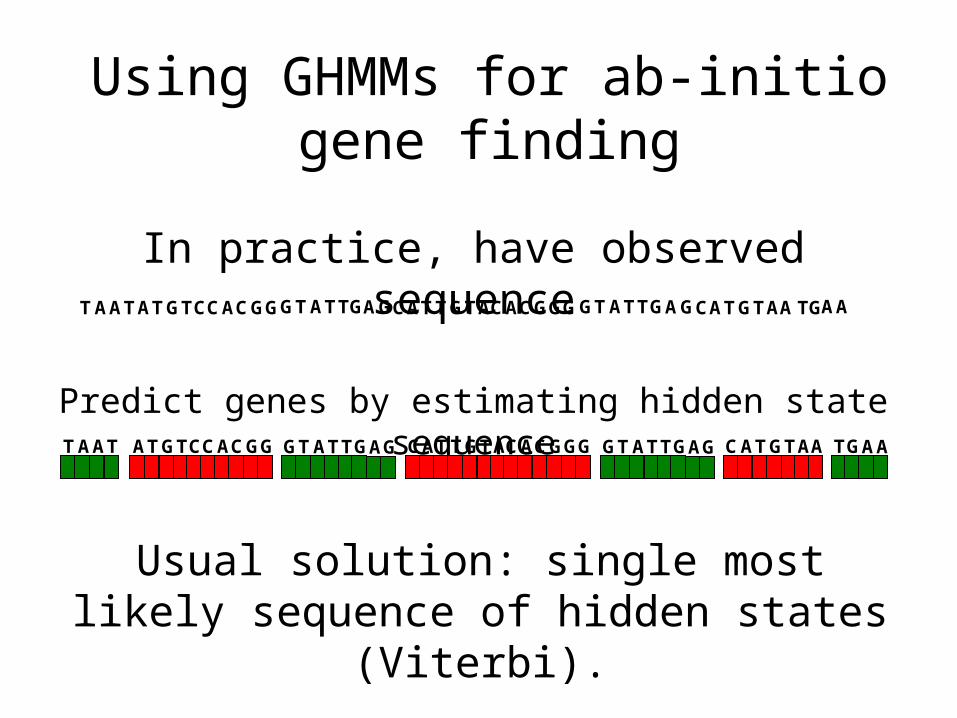
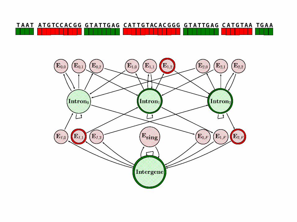
Using GHMMs for ab-initio gene finding
In practice, have observed sequence
Predict genes by estimating hidden state sequence
Usual solution: single most likely sequence of hidden states (Viterbi).
TAATATGTCCACGG TTGTACACGGCA GGTATTGAGGTATTGAG ATGTAAC TGAA
TAAT ATGTCCACGG TTGTACACGGCA G GTATTGAGGTATTGAG ATGTAAC TGAA
TAAT ATGTCCACGG TTGTACACGGCA G GTATTGAGGTATTGAG ATGTAAC TGAA
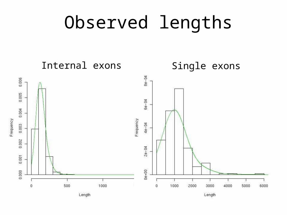
Observed lengths
Internal exons Single exons
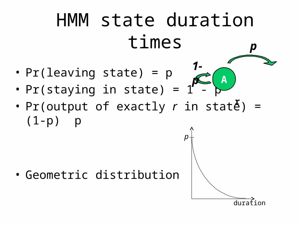
HMM state duration times
p
duration
• Pr(leaving state) = p• Pr(staying in state) = 1 - p• Pr(output of exactly r in state) = (1-p) p
• Geometric distribution
r
A1-p
p
Performance of single organism gene finders
• Estimated ~45,000 genes in the human genome
• Sensitive but not specific
• Bad at accurately identifying exon boundaries

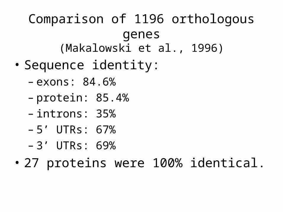
Comparison of 1196 orthologous genes(Makalowski et al., 1996)
• Sequence identity:– exons: 84.6%– protein: 85.4%– introns: 35%– 5’ UTRs: 67%– 3’ UTRs: 69%
• 27 proteins were 100% identical.
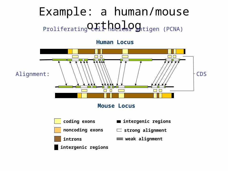
Example: a human/mouse ortholog
Human Locus
Mouse Locus
Alignment: CDS
coding exons
noncoding exons
introns
intergenic regions
strong alignment
weak alignment
intergenic regions
Proliferating cell nuclear antigen (PCNA)
Observation: - Finding the genes will help to find biologically meaningful alignments.-Finding a good alignment will help infinding the genes.
Hidden Markov models– Sequence alignment with Pair HMMs– Gene Prediction with Generalized
HMMs– Both simultaneously with GPHMMs

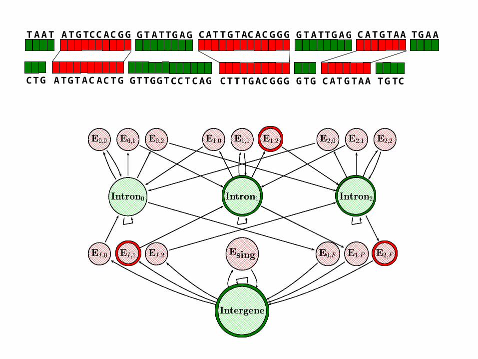
Using GPHMMs for cross-species gene finding
given a pair of syntenic sequences
predict genes by estimating hidden state sequence
Predict exon-pairs using single most likely sequence of hidden states (Viterbi).
TAAT GTATTGAGGTATTGAG TGAA
CTG GTTGGTCCTCAG GTG TGTC
ATGTCCACGG
GA GT TACA TC
TTGTACACGGCA G
T GT ACGCT GG
ATGTAACC
ACC ATGTA
TAAT GTATTGAGGTATTGAG TGAA
CTG GTTGGTCCTCAG GTG TGTC
ATGTCCACGG
GA GT TACA TC
TTGTACACGGCA G
T GT ACGCT GG
ATGTAACC
ACC ATGTA
TAAT GTATTGAGGTATTGAG TGAA
CTG GTTGGTCCTCAG GTG TGTC
ATGTCCACGG
GA GT TACA TC
TTGTACACGGCA G
T GT ACGCT GG
ATGTAAC
ACATGTA
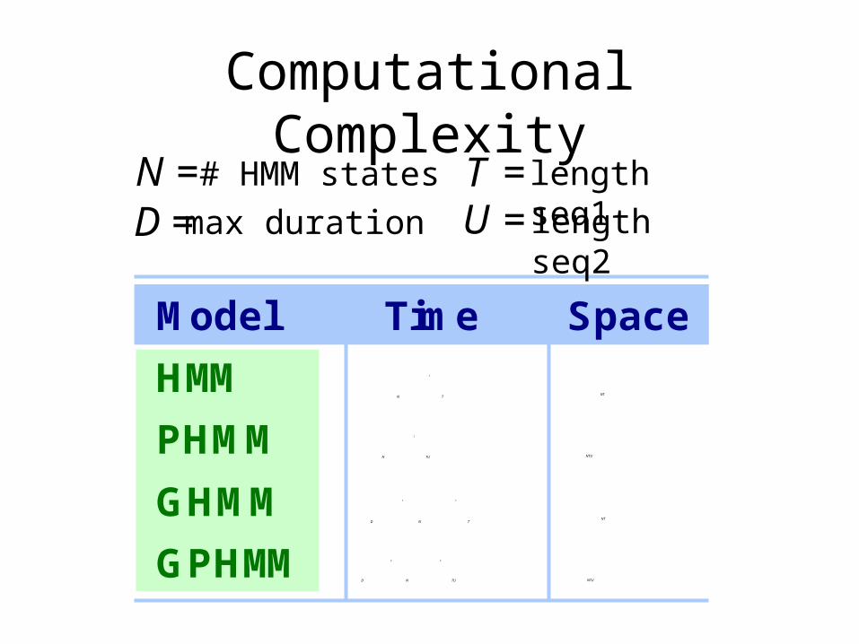
Computational Complexity
Model Time Space
HMMN
2
TNT
PHMMN
2
TU NTU
GHMMD
2
N
2
TNT
GPHMMD
4
N
2
TU NTU
N =# HMM states
D=max duration
T =length seq1U =length seq2
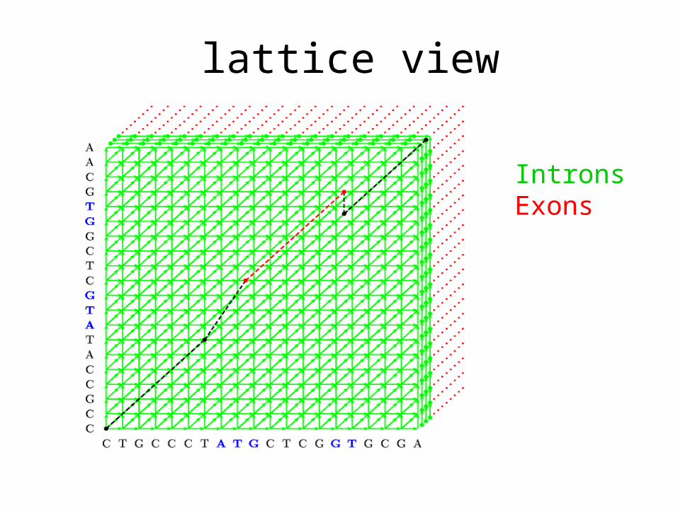
lattice view
IntronsExons
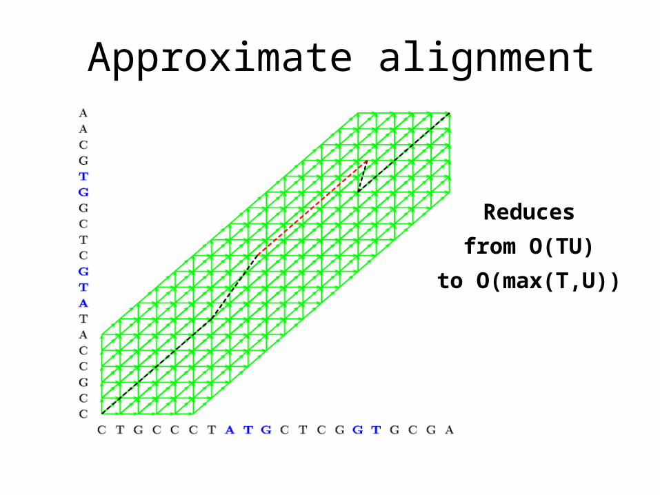
Approximate alignment
Reduces
from O(TU)
to O(max(T,U))

A GPHMM implementationSLAM
• SLAM components– Splice sites (Variable length Markov models).
– Introns and Intergenic regions (2nd order Markov models, independent geometric lengths, CNS states).
– Coding sequences (3-periodic Markov models, generalized length distributions, protein-based pairHMM.)
• Input– Pair of syntenic genomic sequences.
– Approximate alignment.
• Output– CDS predictions in both sequences.
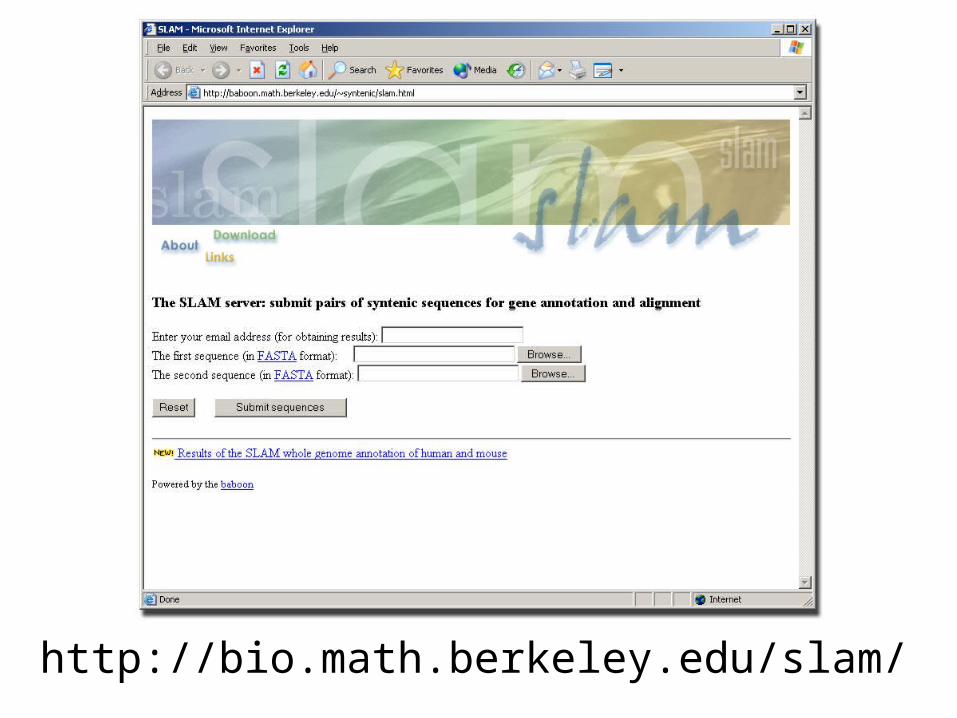
http://bio.math.berkeley.edu/slam/
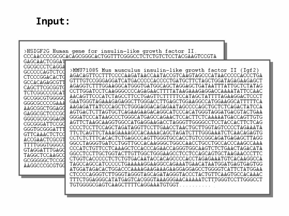
Input:
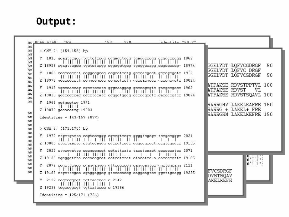
Output:
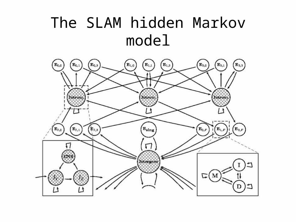
The SLAM hidden Markov model
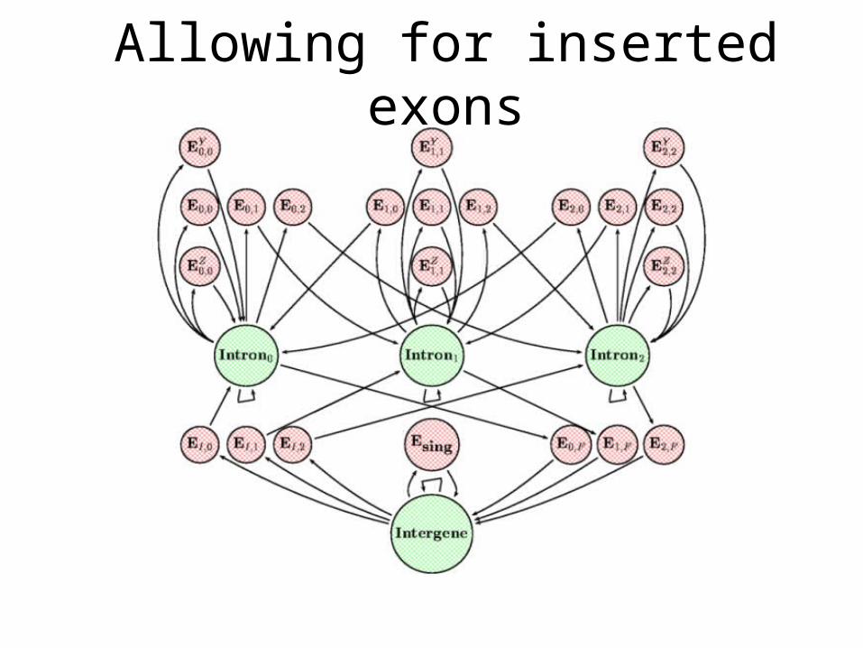
Allowing for inserted exons
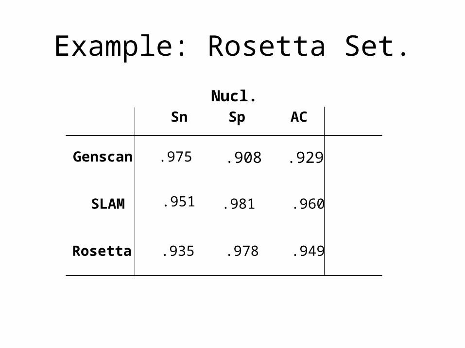
Example: Rosetta Set.
Sn Sp AC
Genscan .908 .929
SLAM
.975
.981 .960
Rosetta .935 .978 .949
Nucl.
.951
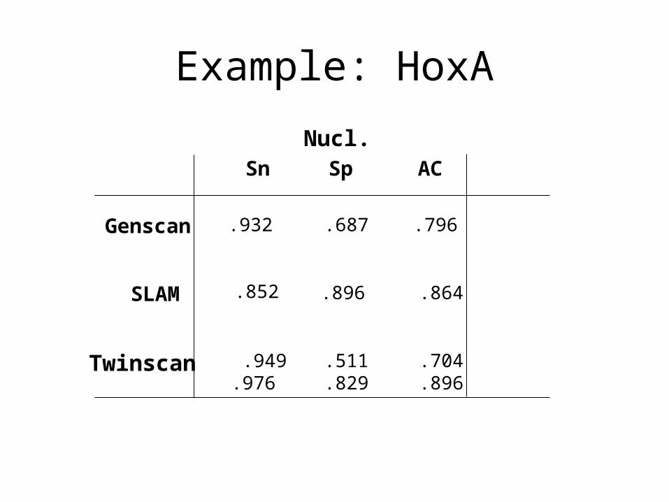
Example: HoxA
Sn Sp AC
Genscan .687 .796
SLAM
.932
.896 .864
Twinscan .949.976
.511
.829.704.896
Nucl.
.852

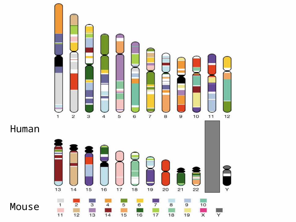
Comparing and annotating the entire
human and mouse genomes
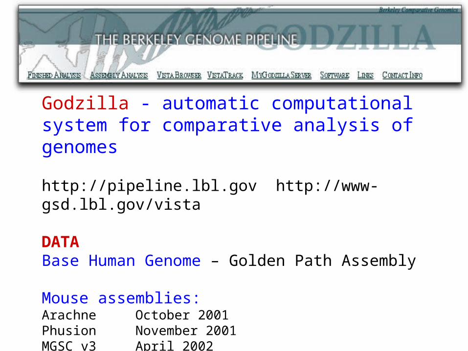
Godzilla - automatic computational system for comparative analysis of genomes
http://pipeline.lbl.gov http://www-gsd.lbl.gov/vista
DATABase Human Genome – Golden Path Assembly
Mouse assemblies:Arachne October 2001 Phusion November 2001 MGSC v3 April 2002
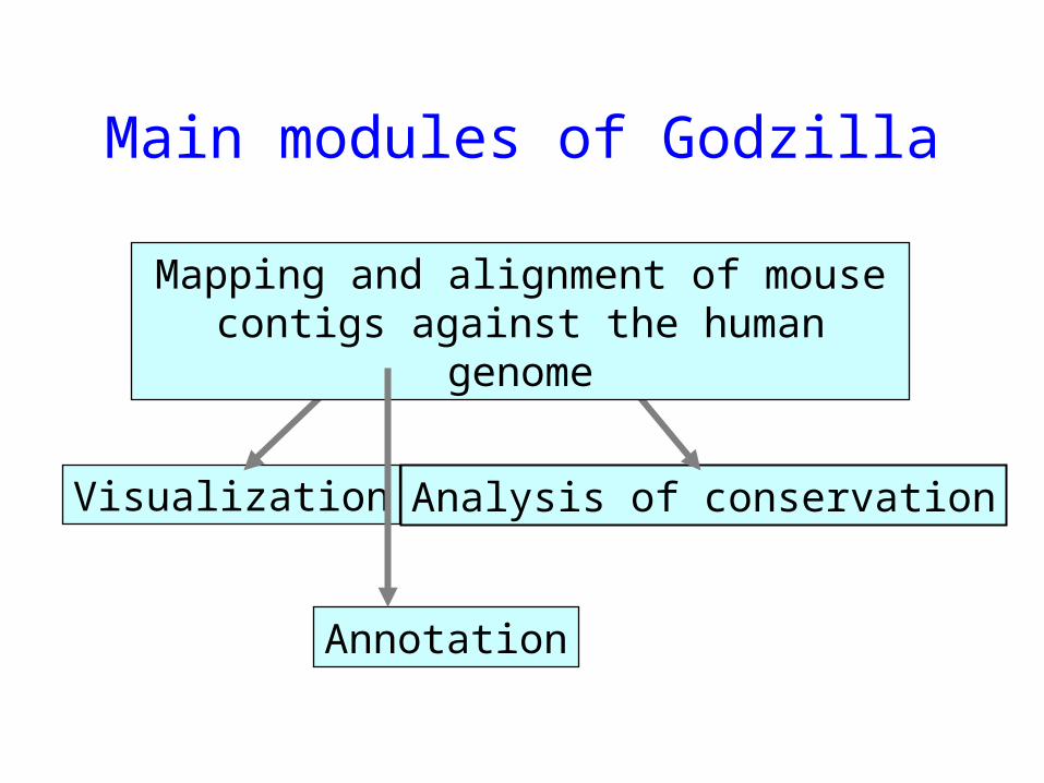
Main modules of Godzilla
Visualization Analysis of conservation
Mapping and alignment of mouse contigs against the human genome
Annotation
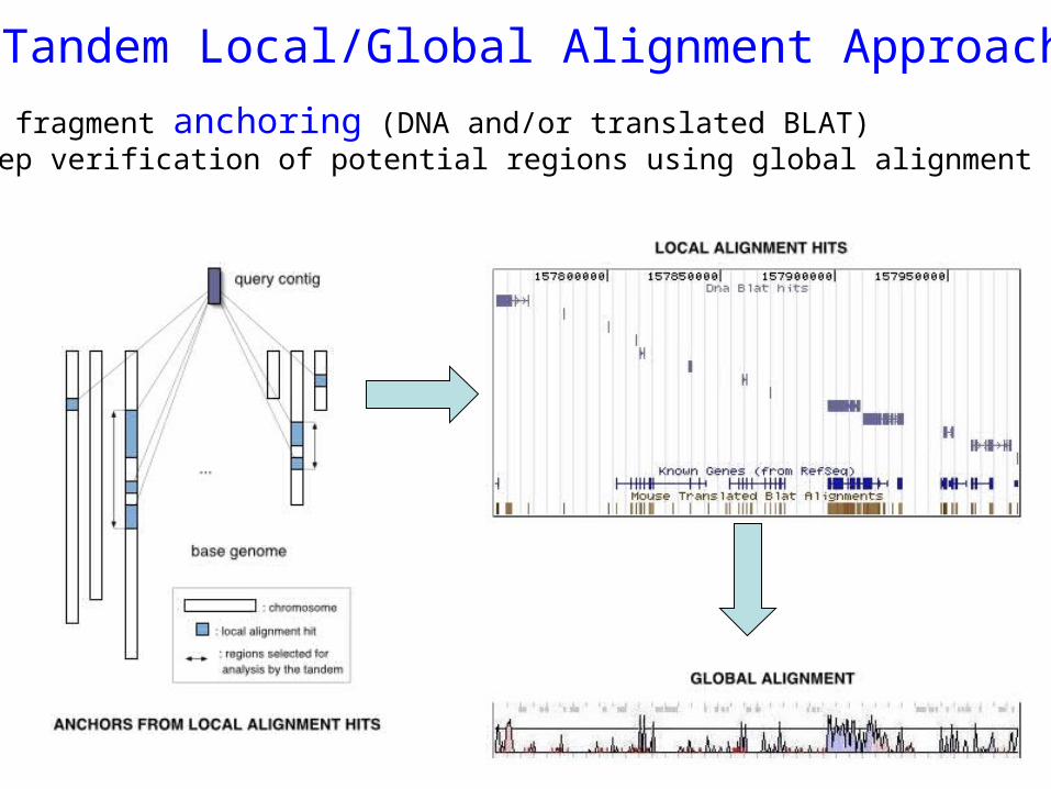
Tandem Local/Global Alignment Approach
Sequence fragment anchoring (DNA and/or translated BLAT) Multi-step verification of potential regions using global alignment (AVID)
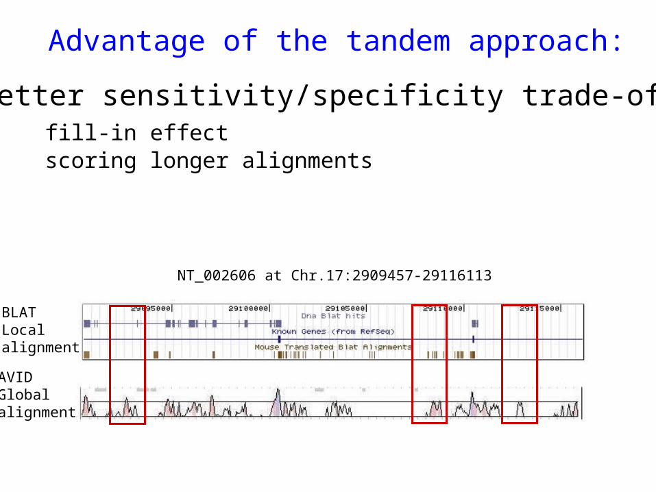
Advantage of the tandem approach:
better sensitivity/specificity trade-offfill-in effectscoring longer alignments
AVIDGlobalalignment
NT_002606 at Chr.17:2909457-29116113
BLATLocal alignment
Our vegetable garden
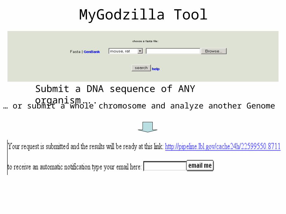
MyGodzilla Tool
Submit a DNA sequence of ANY organism...
… or submit a whole chromosome and analyze another Genome
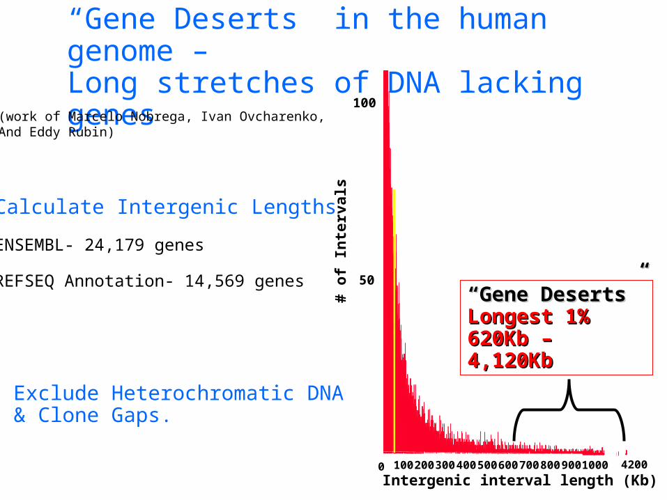
“Gene Deserts” in the human genome –Long stretches of DNA lacking genes
Calculate Intergenic Lengths
ENSEMBL- 24,179 genes
REFSEQ Annotation- 14,569 genes
Exclude Heterochromatic DNA& Clone Gaps.
# o
f In
terv
als
50
100
Intergenic interval length (Kb)0 1002003004005006007008009001000 4200
““Gene Gene Deserts”Deserts”Longest 1% Longest 1% 620Kb – 620Kb – 4,120Kb4,120Kb
(work of Marcelo Nobrega, Ivan Ovcharenko, And Eddy Rubin)
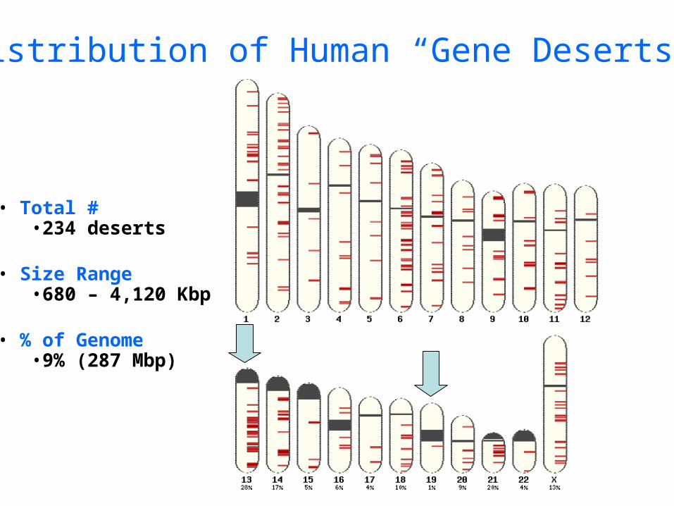
Distribution of Human “Gene Deserts”
• Total #•234 deserts
• Size Range•680 – 4,120 Kbp
• % of Genome•9% (287 Mbp)
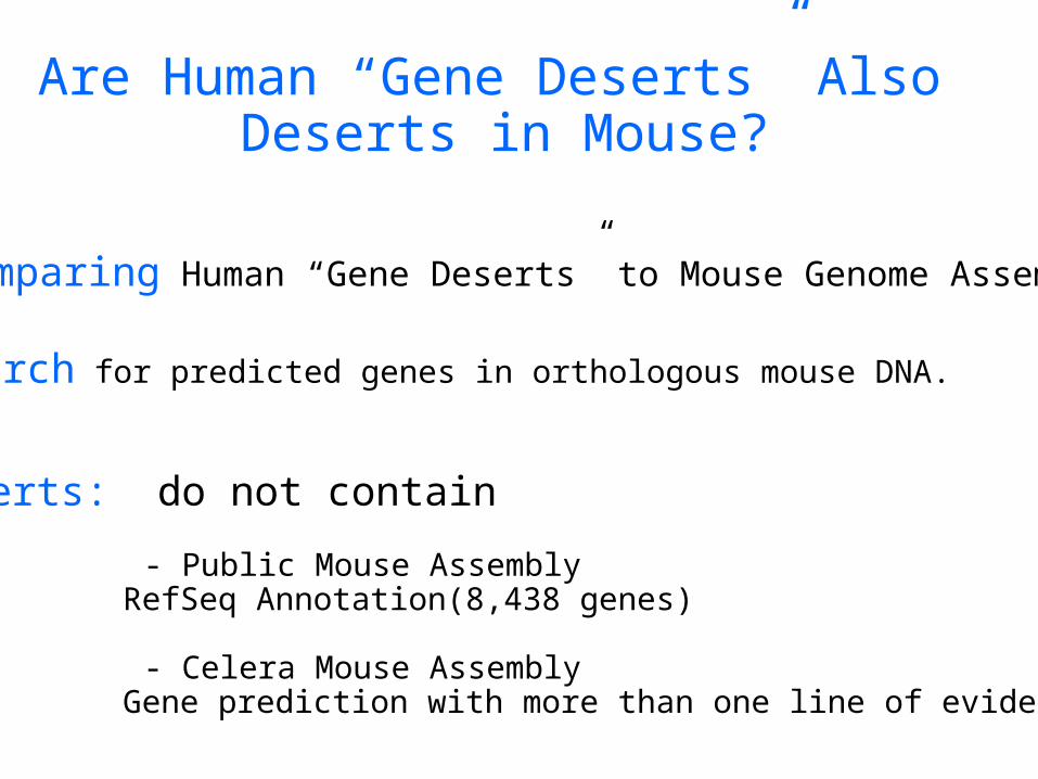
Comparing Human “Gene Deserts” to Mouse Genome Assembly
Search for predicted genes in orthologous mouse DNA.
Are Human “Gene Deserts” Also Deserts in Mouse?
Deserts: do not contain
- Public Mouse AssemblyRefSeq Annotation(8,438 genes)
- Celera Mouse AssemblyGene prediction with more than one line of evidence
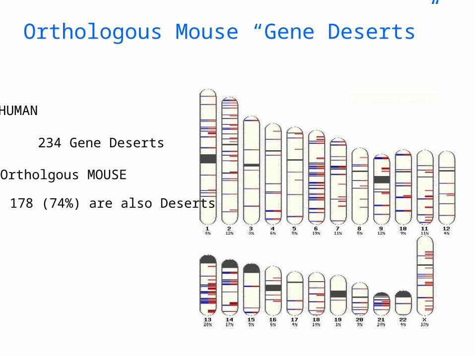
•HUMAN
234 Gene Deserts
• Ortholgous MOUSE
178 (74%) are also Deserts
Orthologous Mouse “Gene Deserts”
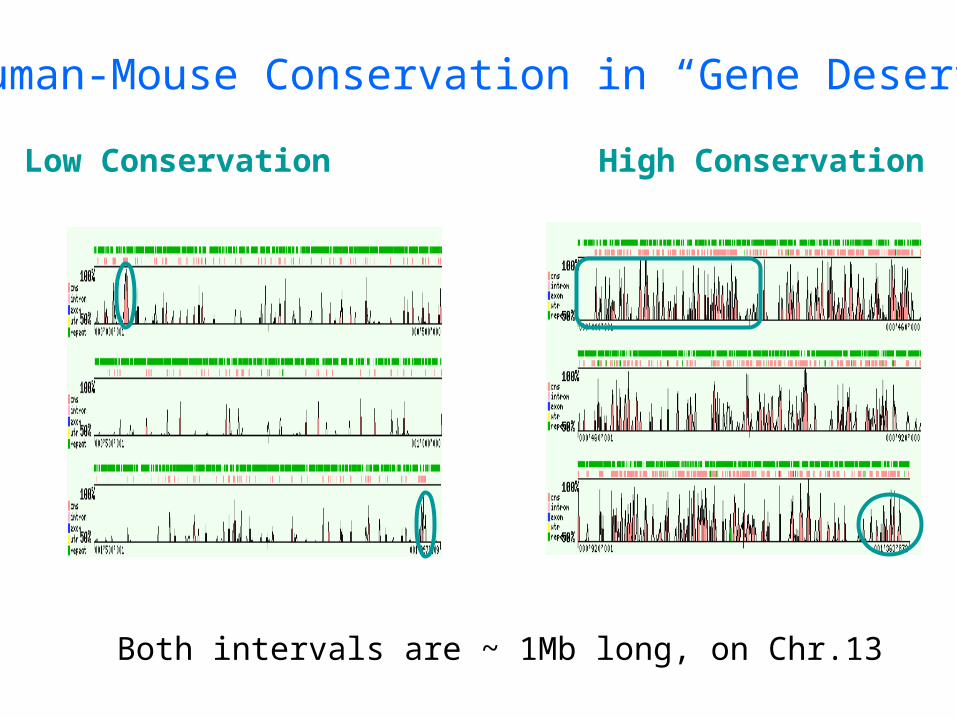
Human-Mouse Conservation in “Gene Deserts”
Low Conservation High Conservation
Both intervals are ~ 1Mb long, on Chr.13
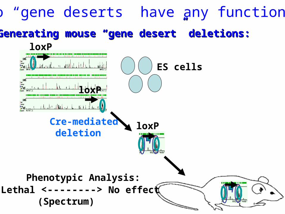
Do “gene deserts” have any function?
Cre-mediated deletion
loxP
loxP
loxP
ES cells
Generating mouse “gene desert” deletions:Generating mouse “gene desert” deletions:
Phenotypic Analysis:Lethal <--------> No effect
(Spectrum)
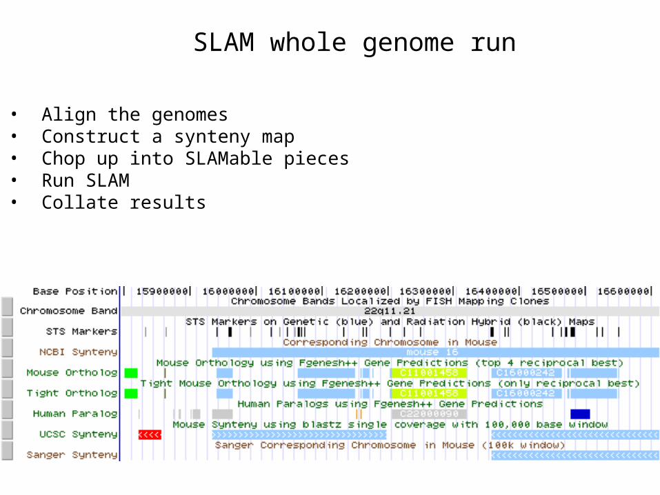
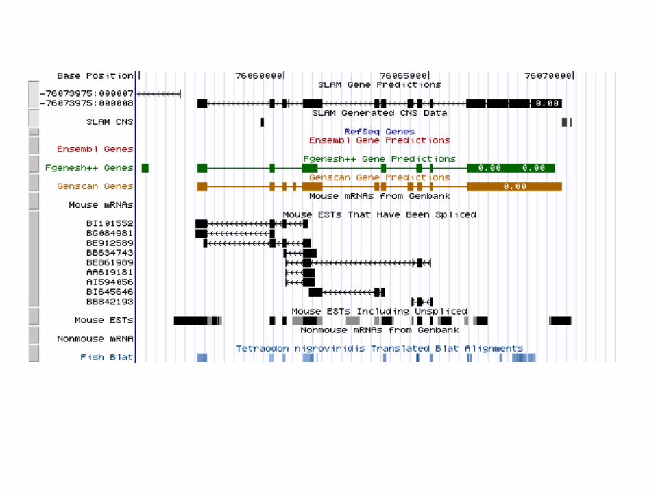
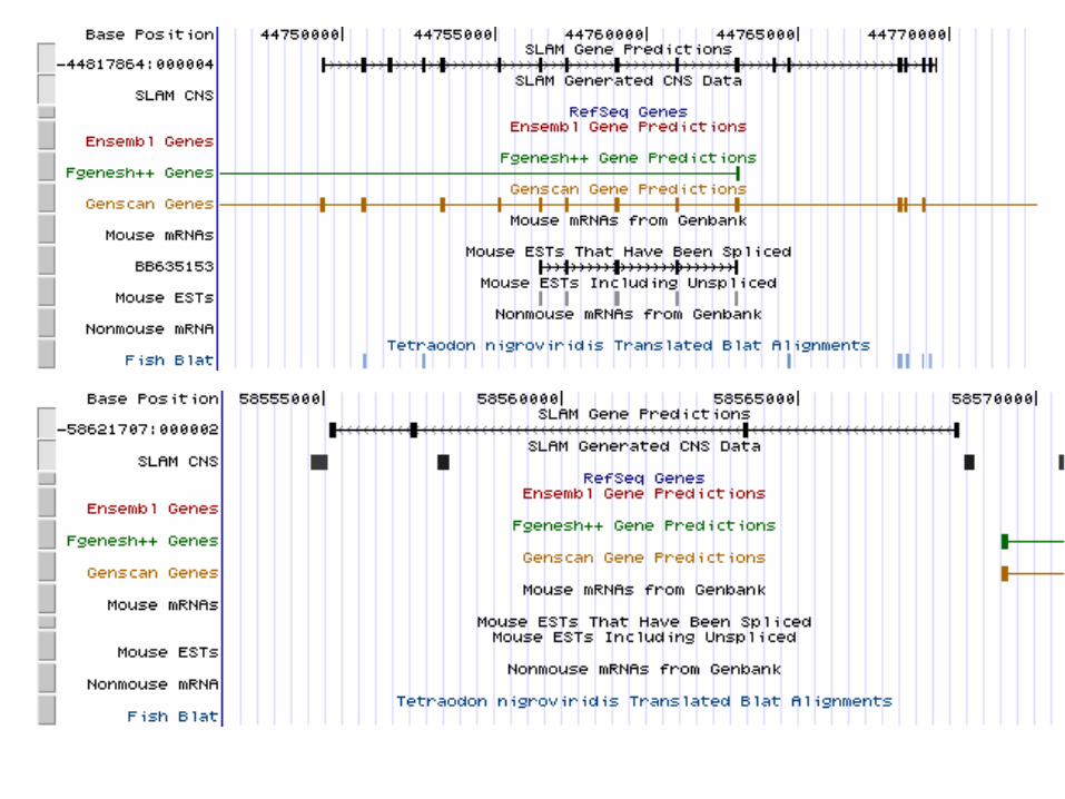
SLAM whole genome run
• Align the genomes• Construct a synteny map• Chop up into SLAMable pieces• Run SLAM• Collate results
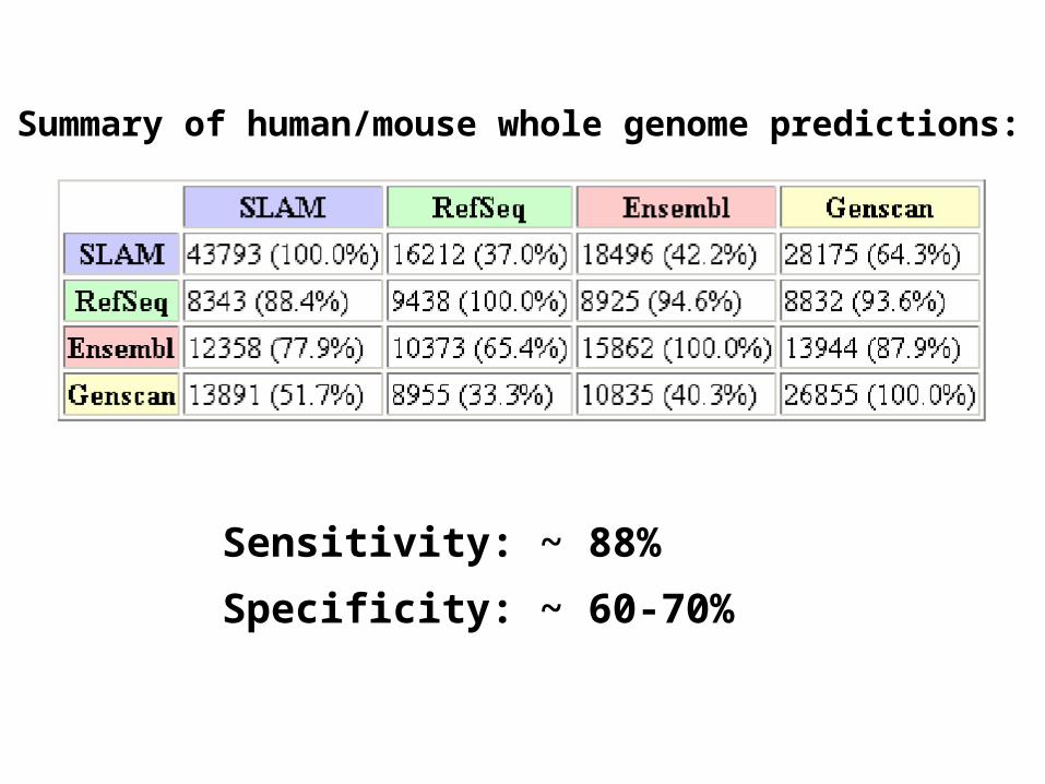
Summary of human/mouse whole genome predictions:
Sensitivity: ~ 88%
Specificity: ~ 60-70%
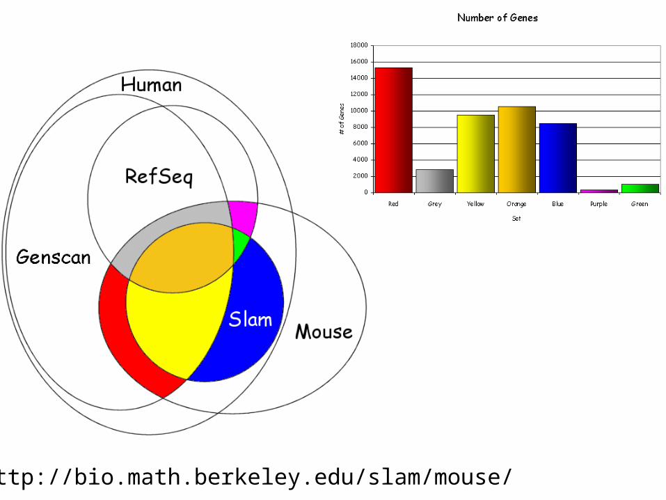
http://bio.math.berkeley.edu/slam/mouse/
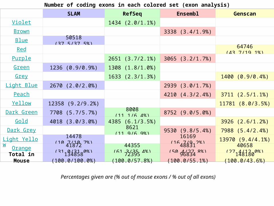
Number of coding exons in each colored set (exon analysis)
SLAM RefSeq Ensembl Genscan
Violet 1434 (2.0/1.1%)
Brown 3338 (3.4/1.9%)
Blue 50518 (37.5/37.5%)
Red 64746 (43.7/19.1%)
Purple 2651 (3.7/2.1%) 3065 (3.2/1.7%)
Green 1236 (0.9/0.9%) 1308 (1.8/1.0%)
Grey 1633 (2.3/1.3%) 1400 (0.9/0.4%)
Light Blue 2670 (2.0/2.0%) 2939 (3.0/1.7%)
Peach 4210 (4.3/2.4%) 3711 (2.5/1.1%)
Yellow 12358 (9.2/9.2%) 11781 (8.0/3.5%)
Dark Green 7708 (5.7/5.7%) 8008 (11.1/6.4%) 8752 (9.0/5.0%)
Gold 4018 (3.0/3.0%) 4385 (6.1/3.5%) 3926 (2.6/1.2%)
Dark Grey 8621 (11.9/6.9%) 9530 (9.8/5.4%) 7988 (5.4/2.4%)
Light Yellow 14478 (10.7/10.7%) 16169 (16.7/9.2%) 13970 (9.4/4.1%)
Orange 41872 (31.0/31.0%) 44355 (61.3/35.4%) 48831 (50.4/27.8%) 40658 (27.4/12.0%)
Total in Mouse 134858 (100.0/100.0%) 72395 (100.0/57.8%) 96834 (100.0/55.1%) 148180 (100.0/43.6%)
Percentages given are (% out of mouse exons / % out of all exons)
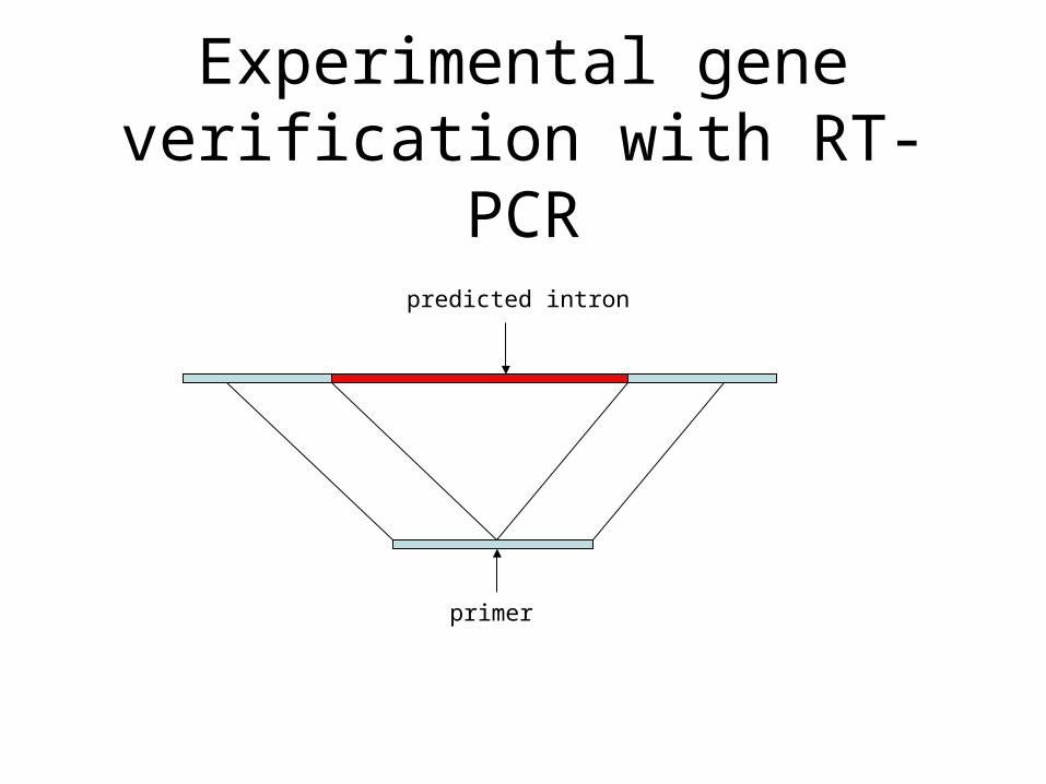
Experimental gene verification with RT-PCR
predicted intron
primer
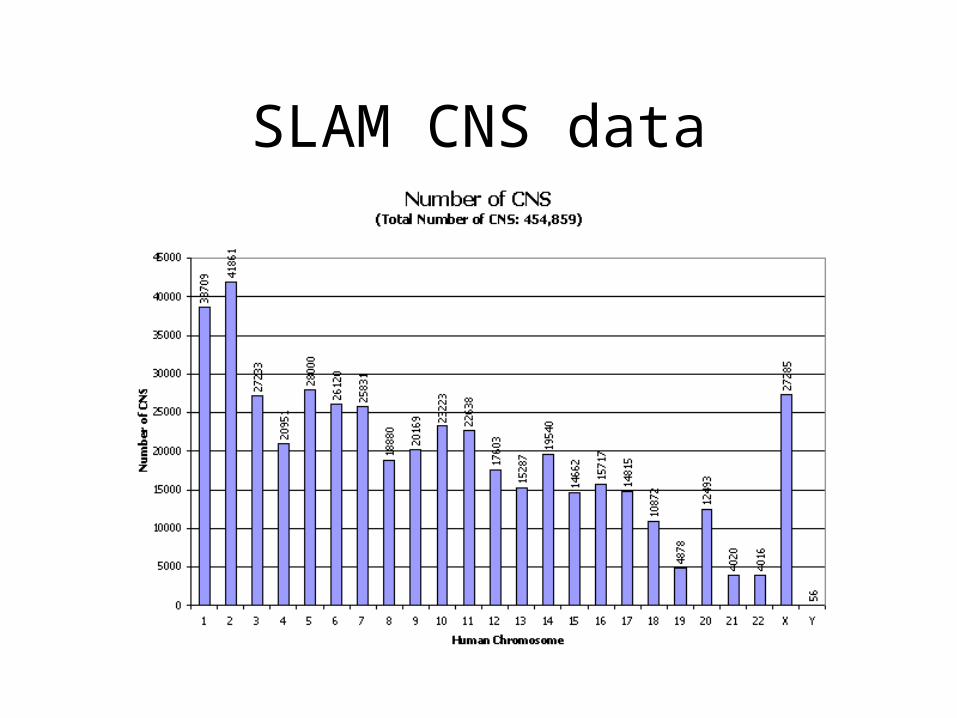
SLAM CNS data
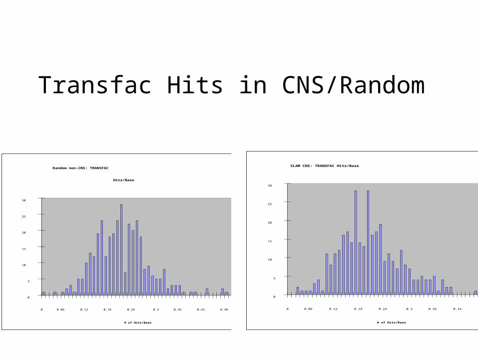
Random non-CNS: TRANSFAC
Hits/Base
0
5
10
15
20
25
30
0 0.06 0.12 0.18 0.24 0.3 0.36 0.42 0.48 0.54 0.6
# of Hits/Base
Frequency
SLAM CNS: TRANSFAC Hits/Base
0
5
10
15
20
25
30
0 0.06 0.12 0.18 0.24 0.3 0.36 0.42 0.48 0.54 0.6
# of Hits/Base
Frequency
Transfac Hits in CNS/Random
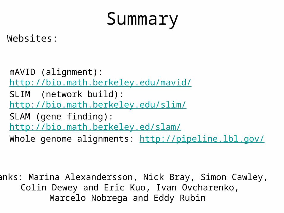
Summary
Thanks: Marina Alexandersson, Nick Bray, Simon Cawley, Colin Dewey and Eric Kuo, Ivan Ovcharenko,
Marcelo Nobrega and Eddy Rubin
mAVID (alignment): http://bio.math.berkeley.edu/mavid/SLIM (network build): http://bio.math.berkeley.edu/slim/SLAM (gene finding): http://bio.math.berkeley.ed/slam/Whole genome alignments: http://pipeline.lbl.gov/
Websites: