CIRJE-F-624 Generating a Target Payoff Distribution with

CIRJE Discussion Papers can be downloaded without charge from:

http://www.cirje.e.u-tokyo.ac.jp/research/03research02dp.html

Discussion Papers are a series of manuscripts in their draft form. They are not intended for

circulation or distribution except as indicated by the author. For that reason Discussion Papers may

not be reproduced or distributed without the written consent of the author.

CIRJE-F-624

Generating a Target Payoff Distributionwith the Cheapest Dynamic Portfolio:

An Application to Hedge Fund Replication

Akihiko TakahashiUniversity of Tokyo

Kyo YamamotoGCI Asset Management, Inc.

June 2009; Revised in March 2010 and February 2013

Generating a Target Payoff Distributionwith the Cheapest Dynamic Portfolio:

An Application to Hedge Fund Replication∗

Akihiko Takahashi†and Kyo Yamamoto‡

First draft: June 16, 2009This version: February 17, 2013

∗This research is supported by CARF (Center for Advanced Research in Finance) andthe global COE program “The research and training center for new development in math-ematics.” We are very grateful to two anonymous referees for their precious comments,which have improved the previous version of this paper substantially. Also, we thankHideki Yamauchi and Takahiko Suenaga at GCI Asset Management Inc. and TetsuyaAoki at GCI Investment Management Singapore Pte. Ltd. for their constant support. Allthe contents expressed in this research are solely those of the authors and do not repre-sent any views or opinions of any institutions. The authors are not responsible or liablein any manner for any losses and/or damages caused by the use of any contents in thisresearch. Takahashi and Yamamoto (2010) is the summary of this research. It is basedon the presentation entitled “A New Hedge Fund Replication Method with the dynamicOptimal Portfolio” at Global Conference on Business and Finance 2010, Kailua-Kona,Hawaii.

†Graduate School of Economics, The University of Tokyo‡GCI Asset Management, Inc.

1

Abstract

This paper provides a new method to construct a dynamic opti-mal portfolio for asset management. This method generates a targetpayoff distribution using the cheapest dynamic trading strategy. Asa practical example, the method is applied to hedge fund replica-tion. This dynamic portfolio strategy is regarded as an extension of ahedge fund replication methodology that was developed by Kat andPalaro (2005a, b) and Papageorgiou, Remillard and Hocquard (2008)to address multiple trading assets with both long and short positions.Empirical analyses show that such an extension significantly improvesthe performance of replication in practice.

1 Introduction

Modern portfolio theory has been applied to asset management in practicesince the seminal works of Markowitz (1952) and Merton (1969, 1971). Thispaper considers a tractable portfolio construction problem for portfolio man-agers. While Markowitz (1952) proposed a portfolio optimization methodwhere the portfolio that minimizes its variance under a given expected returnis chosen, this paper presents a method to create the dynamic portfolio thatattains a target payoff distribution with the minimum cost in a continuous-time complete market. Moreover, this cost minimization problem is shownto be equivalent to a standard expected utility maximization problem thatwas studied by Merton (1969, 1971).

Practical performance evaluations of mutual and hedge funds are usuallybased upon the basic statistics of their returns, such as certain orders ofmoments and their combinations (e.g., Sharpe ratio). In particular, manyresearchers have pointed out that hedge fund returns exhibit non-normality(see, for example, Malkiel and Saha (2005) and Hakamada et al. (2007)).Thus, high orders of moments should be also considered for investment inhedge funds (see, for example, Gregoriou and Kaiser (2006) and Cvitanic,Polimenis and Zapatero (2008)). Dybvig (1988a) proposed a distributionalanalysis approach to evaluating investment performances. This approachmodified the Sharpe and Jensen measures by incorporating all of the momentsof a return distribution.

Our method extends the distributional analysis approach initiated byDybvig (1988a). Theorem 1 in Dybvig (1988a) claims that the cheapest

2

way to attain a given payoff is to allocate terminal wealth in the reverseorder of the state price density in an equally probable finite state completemarket. This article extends that claim to a continuous-time complete marketframework. The uniqueness of the cheapest payoff is also proven. Theorem2 in Dybvig (1988a) asserts that a trading strategy maximizes an increasingand concave von Neumann-Morgenstern utility in an equally probable finitestate complete market if and only if it is the cheapest strategy among thosethat generate the same payoff distribution. This paper shows a similar resultholds in a continuous-time complete market setting, as well. Hence, it isensured that our portfolio optimization problem is equivalent to an expectedutility maximization problem.

Dybvig (1988a) intended an extension of the capital asset pricing model(CAPM) and techniques for evaluating investment performance and testingits efficiency. In addition, Dybvig (1988b) used the distributional analysis toinvestigate the efficiency of the standard dynamic trading strategies that arefollowed by practitioners. However, this paper applies the idea to creatingthe dynamic optimal portfolio that achieves a target payoff distribution. Fora target distribution, there is an interesting example: hedge fund replication.

Hedge fund replication products appeared in financial markets afterthe late 2000s. Large investment banks and asset management companieslaunched such products one after another. They have been developing theirown original methods by employing highly sophisticated financial models andstatistical methods. Some have developed replication techniques by collabo-rating with the pioneers in hedge fund research (see, for example, Takahashiand Yamamoto (2009) or Tuchschmid et al. (2010, 2012)). These productsovercome some of the disadvantages of hedge fund investment: high cost, lowtransparency, and low liquidity. The importance of transparency and liquid-ity has been recognized since the subprime and Lehman shocks. Therefore,these products have gained increased attention. Tuchschmid et al. (2010,2012) examined the performances of existing hedge fund clone products.

Many financial firms offer the clones of various investment strategies.Most of the replication products attempt to replicate the performances ofaggregate composite hedge fund indexes from HFR, Dow Jones Credit Suisse,and so on. Others attempt to replicate the performances of some specific al-ternative investment strategies, such as equity long/short or market-neutral.

The existing methodologies for hedge fund replication can be catego-rized into the following three approaches: the rule-based, factor-based, anddistribution-replicating approach. The rule-based approach mimics the typi-

3

cal trading strategies that are employed by hedge funds. The trading rules inDuarte et al. (2007) can be regarded as rule-based fixed-income hedge fundclone techniques.

Factor-based cloning attempts to replicate the risk exposures of the targetfund. If this method succeeds, then the return of the clone tracks that ofthe target fund on a month-to-month basis. Lo and Hasanhodzic (2007)and Fung and Hsieh (2007a, 2007b) studied this approach. Factor analysistechniques that have been developed for hedge funds since the late 1990s,such as that of Fung and Hsieh (1997, 2000, 2001) and Agarwal and Naik(2004), are directly applied to the replication.

The distribution-replicating approach aims to replicate the distributionsof hedge fund returns. Amin and Kat (2003) first attempted this replication.However, hedge funds attract investors not only by their return distributionsbut also by their low correlations with the returns of traditional asset classes,such as stocks and bonds. Therefore, Kat and Palaro (2005a, b) extended themethod to replicate both the distribution and the dependence structure onthe investor’s existing portfolio. Kat and Palaro (2005a, b) tried to replicatethem through a dynamic trading of the investor’s existing portfolio (approx-imated by a portfolio of stock index futures and bond futures) and anotherasset (replicating instrument). Papageorgiou et al. (2008) proposed an alter-native way to perform Kat-Palaro’s replication methodology by utilizing ahedging scheme for options in an incomplete market. The payoff distributionmodel can be applied to not only hedge fund replication but also to otherinvestment strategies and risk managements. For example, Hocquard et al.(2012) applied it to portfolio insurance.

This article extends the work of Kat and Palaro (2005a, b) and Papa-georgiou et al. (2008). While the methods developed by the two researchpapers use one replicating instrument with long positions only, our methodallows multiple replicating instruments with both long and short positionsfor creating a replicating portfolio. With regard to practical applications,this paper replicates the return distributions of three different hedge fundstrategies: managed futures, multi-strategy, and global macro indices fromDow Jones Credit Suisse. Such fund managers are seeking attractive in-vestment opportunities in financial markets around the world. They employdynamic trading strategies, including leverage and short sales, to make profitsfrom such opportunities. Our methodology is able to reflect their investmentbehaviors. Managed futures funds gained high returns by taking short po-sitions on risky assets in the months immediately following the bankruptcy

4

of Lehman Brothers. As this new replication method allows for short posi-tions, it is much easier to replicate a managed futures fund that shows goodperformance even in substantial bear markets. Historical out-of-sample sim-ulations show that our scheme provides much better performances than dothe replications with one replicating instrument and its long positions only.

This paper is organized as follows. The following section briefly reviewsthe existing distribution replication methodology with one replicating in-strument and its long positions only. Section 3 describes the new dynamicportfolio optimization method, which is an extension of the distribution repli-cation method to multiple replicating instruments with both long and shortpositions. Then, Section 4 applies the new method to the replication of hedgefund indexes. Section 5 concludes this paper. Finally, the Appendix gives theproofs of the theorems as well as the derivation of the dynamic replicatingportfolios.

2 Review of the Existing Distribution Repli-

cation Methodology

Before describing the new dynamic portfolio optimization method, let us re-view the distribution replication methodology developed by Kat and Palaro(2005a, b) and Papageorgiou et al. (2008), which helps us to understandthe motivation of this study. Consider an investor who has been investingin traditional assets, such as stocks and bonds, and who plans to invest in ahedge fund. Assume that he/she is attracted to the hedge fund because of itsreturn distribution and the structure of dependence upon his/her portfolio.Kat and Palaro (2005a, b) proposed to replicate the return distribution ofthe hedge fund and its dependence structure on the investor’s existing port-folio by a dynamic trading strategy of the investor’s portfolio (approximatedby a portfolio of stock index futures and bond futures) and another asset(replicating instrument).

Let S0 be a risk-free asset, S1 be the investor’s existing portfolio, and S2

be a replicating instrument. Assume that S1 is also tradable. Let 0 and Tbe the start and terminal dates of the investment, respectively (for exam-ple, they are assumed to be the start and end of the month, respectively).Although Papageorgiou et al. (2008) assumed an incomplete market, thispaper assumes a complete market. Suppose that the financial assets follow

5

stochastic differential equations (SDEs)

dS0t = rtS

0t dt,

dS1t = µ1

tS1t dt+ σ11

t S1t dW

1t ,

dS2t = µ2

tS2t dt+ σ21

t S2t dW

1t + σ22

t S2t dW

2t ,

where W 1t and W 2

t are independent Wiener processes, and rt, µit, and σij

t

(i, j = 1, 2) satisfy some measurability and integrability conditions. Normal-ize the initial asset values so that S0

0 = S10 = S2

0 = 1. Then, the log returnsof S1 and S2 are represented as R1

T = logS1T and R2

T = log S2T , respectively.

Let RT be the random variable that represents the log return of thetarget hedge fund. Kat and Palaro (2005a, b) proposed to replicate the jointdistribution of

(R1

T , RT

)through the dynamic trading of S1 and S2. They

created a payoff function of S1 and S2 that has the same joint distribution asthe target hedge fund, and they then replicated the payoff using a dynamictrading strategy for S1 and S2. They found function g, which satisfies thefollowing equation.

P(R1

T ≤ a, g(R1

T , R2T

)≤ b)= P(R1

T ≤ a,RT ≤ b) for any a, b,

or equivalently,

P(g(R1

T , R2T

)≤ b∣∣R1

T = a)= P(RT ≤ b|R1

T = a) for any a, b.

The function g(·, ·) is given by

g(a, b) = F−1RT |a(FR2

T |a(b)),

where FRT |a and FR2T |a are the conditional distribution functions ofRT andR2

T

under R1T = a. As the function of the asset prices, the payoff is represented

asg(S1

T , S2T ) = exp

g(logS1

T , log S2T

). (1)

Payoff g(S1T , S

2T ) has the same joint distribution with the investor’s portfolio

as does the target hedge fund.Once one has obtained the payoff function, then the replicating strategy

encounters the same problem with pricing and hedging derivatives. Thedynamic replicating strategy is given by the delta-hedging strategy of thepayoff g(S1

T , S2T ). If the initial cost for the trading strategy is less (more)

6

than one, then the target payoff distribution is realized by a lower (higher)cost. The remaining (shortage of) money is invested (funded) in the risk-freeasset. This means that the shape of the probability density function can bereplicated, but the mean return is higher (lower) than the target fund by thedifference of the initial cost. In this case, the replicating instrument does(does not) include a greater investment opportunity than does the targethedge fund. Note that the payoff function g(·, ·) is increasing with respectto the second argument. The delta-hedging strategy therefore never takes ashort position for S2. In pp. 17-18 of Kat and Palaro (2005a), the authorsclaim that users of this method should choose the replicating instrument S2,which includes a positive expected return factor that is uncorrelated to thereturn of the investor’s portfolio. The long positions for S2 are thus justified.Therefore, the choice of a replicating instrument is a very important problem.

As just described, this methodology can replicate the shape of the prob-ability density function, but it cannot fit the mean. If you found a greaterinvestment opportunity than the target fund, the mean return would be su-perior, and vice versa. Therefore, the usage of only one asset is restrictive.Papageorgiou et al. (2008) synthesized multiple assets to create one repli-cating instrument by equal-weighing, but such a portfolio would not alwaysbe optimal. The extension of the investment universe would bring in highermean returns. The dynamic portfolio strategy presented in the next sectioncan be considered to be an extension of this distribution replication methodto multiple replicating instruments with both long and short positions.

3 The Cheapest Dynamic Portfolio that Gen-

erates a Target Payoff Distribution

Let us begin with a complete probability space (Ω,F ,P) with n-dimensionalstandard Brownian motion Wt = (W 1

t , · · · ,W nt )

′, 0 ≤ t ≤ T , where ′ repre-sents transposition so that Wt is a column vector. W0 = 0 is almost surelysatisfied. Let FW

t 0≤t≤T be the filtration generated by Wt. This paper usesthe augmented filtration

Ft = σ(FWt ∪N ) for any t < T,

where N denotes P-null subsets of FWT .

Let S0 be a risk-free asset, S1 be the investor’s existing portfolio, andS2, · · · , Sn be risky assets. Suppose that the price processes of the financial

7

assets Si (i = 0, · · · , n), SitTt=0, follow SDEs

dS0t = rtS

0t dt, (2)

dSit = µi

tSitdt+

i∑j=1

σijt S

itdW

jt (i = 1, · · · , n), (3)

where rt, µit, and σ

ijt are progressively measurable and satisfy∫ T

0

|rt|dt <∞ a.s.,

∫ T

0

|µit|dt <∞ a.s.,∫ T

0

(σijt )

2dt <∞ a.s.

for any 1 ≤ j ≤ i ≤ n.All of the initial asset values are normalized, so that S0

0 = · · · = Sn0 = 1.

The following notations for n-dimensional vectors and an n × n matrix areintroduced. St = (S1

t , · · · , Snt )

′, µt = (µ1t , · · · , µn

t )′, 1 = (1, · · · , 1)′, and

σt =

σ11t O...

. . .

σn1t · · · σnn

t

,

where ′ represents transposition so that St, µt and 1 are column vectors.Suppose that σt is almost surely invertible. There then exists the unique

market price of the riskθt = σ−1

t (µt − rt1).

In other words, the financial market is complete. The financial market isdenoted by M = (r, µ, σ).

In a complete market M, the unique state price density process is givenby

Ht = exp

−∫ t

0

rudu−1

2

∫ t

0

||θu||2du−∫ t

0

θ′udWu

.

8

The no-arbitrage price of any FT -measurable payoff X is given by x =E[HTX]. X can be replicated by a dynamic trading of the financial assetswith initial cost x (see, for example, Karatzas and Shreve (1998)).

When multiple risk assets are tradable, then there are infinitely manypayoffs that have a target distribution. This paper proposes to choose thecheapest of these payoffs. Dybvig (1988a) showed that the cheapest way toattain a given payoff is to allocate the terminal wealth in the reverse order ofthe state price density in an equally probable finite state complete market. Aswill be seen later, this claim is also valid in our setting under some conditions.In the following, we find the cheapest payoffs that attain a target marginaldistribution and a joint distribution with the investor’s existing portfolio.

First, let us find the cheapest payoff that has a target marginal distribu-tion. Let ξ be a random payoff that has a target distribution. For conve-nience, the minus logarithm state price density process Lt is introduced asfollows.

Lt = − logHt =

∫ t

0

rudu+1

2

∫ t

0

||θu||2du+∫ t

0

θ′udWu. (4)

Because Arrow-Debreu securities are tradable in a complete market, this pa-per proposes to create a payoff using HT (or LT ). Let Fξ and FLT

denote thedistribution functions of ξ and LT , respectively. Assume that Fξ is an invert-ible function. If X is defined as follows, then X has the same distribution asξ.

X = f(LT ), (5)

wheref(l) = F−1

ξ

(FLT

(l)).

Because F−1ξ and FLT

are increasing, the payoff X increases in LT , andtherefore it is in the reverse order of the state price density HT . Thus, X isthe cheapest payoff among the payoffs that have the same distribution as ξ.The next theorem asserts that X is the unique, cheapest payoff among therandom variables that has the same distribution as ξ.

Theorem 1 Assume that ξ is a positive FT -measurable random variable,and Fξ and FLT

are continuous and strictly increasing. In a complete marketM, the unique cheapest payoff X that has the same distribution as ξ is givenby equation (5).

9

Proof. See Appendix 6.1.

Additionally, the choice of the cheapest payoff for some marginal distri-bution can be justified in terms of the expected utility maximization theory.It can be shown that the cost minimization for a marginal payoff distributionis equivalent to a von Neumann-Morgenstern utility maximization. Dybvig(1988a) proved this claim in the equally probable finite state setting. Thenext theorem proves this claim in a continuous-time framework.

Theorem 2 Assume that ξ is a positive FT -measurable random variable,and Fξ and FLT

are continuous and strictly increasing. If X is the cheapestpayoff that has the same distribution with ξ (i.e., X is defined by equation(5)), then in a complete market M, there exists a strictly increasing andstrictly concave von Neumann-Morgenstern utility function u(·), such that(a) limz→+0 u

′(z) = +∞, (b) limz→+∞ u′(z) = 0, and the dynamic tradingstrategy that attains payoff X is the optimal investment strategy for u(·).

Conversely, if a dynamic trading strategy maximizes a strictly increas-ing and strictly concave von Neumann-Morgenstern utility function u(·) thatsatisfies conditions (a) and (b), then it attains the cheapest payoff for somedistribution.


Next, let us find the cheapest payoff that has a target joint distributionwith the investor’s existing portfolio, S1. Denote the conditional distributionfunctions of ξ and LT under condition S1

T = s by Fξ|s and FLT |s, respectively.Assume that Fξ|s is invertible for any s. If X is defined as follows, then(S1

T , X) has the same joint distribution as (S1T , ξ).

X = g(S1T , LT ), (6)

whereg(s, l) = F−1

ξ|s (FLT |s(l)).

Because F−1ξ|s and FLT |s are increasing, the payoff X increases in LT , and it

is therefore in the reverse order of the state price density, HT . Thus, X isthe cheapest payoff among the payoffs that have the same joint distributionwith the investor’s existing portfolio as ξ. The next theorem asserts thatX is the unique, cheapest payoff among the random variables whose jointdistributions with S1

T are the same as ξ.

10

Theorem 3 Assume that ξ is a positive FT -measurable random variable,and Fξ|s and FLT |s are continuous and strictly increasing for any s > 0.In a complete market M, the unique cheapest payoff X among the randomvariables whose joint distributions with S1

T are the same as ξ is given byequation (6).


Let us derive the dynamic portfolio that replicates the cheapest payoffs.Let πi

t (i = 0, · · · , n) represent the money amount that is invested in asseti at time t. The n-dimensional vector πt is defined by πt = (π1

t , · · · , πnt )

′,which denotes a portfolio of risky assets. Let x be the initial cost that isrequired to realize the cheapest payoff XT for some payoff distribution. Theinitial cost x is invested in the financial assets by a dynamic self-financingtrading strategy to generate the payoff XT . In other words, the portfoliovalue at time t, Xt, satisfies

Xt = π0t + π′

t1,

for any t. In a differential form, this is expressed as

dXt = rtXtdt+ π′t(µt − rt1)dt+ π′

tσtdWt.

The dynamic portfolio can be obtained concretely for the case of Marko-vian coefficients. See Appendix 6.4 for details. The following discussion inthis paper applies a special case of Appendix 6.4, where r, µ, and σ are deter-ministic functions of the time t. The next proposition provides the dynamicreplicating portfolios in this case.

Proposition 1 Assume that r, µ and σ are deterministic functions of thetime t. Then, in a complete market M, the dynamic portfolio that generatespayoff f(LT ) is given by

πMt = σ′(t)−1ϕM

t , (7)

where

ϕMt =

θ(t)

Ht

Et[HTf′(LT )]. (8)

The portfolio that attains the payoff g(S1T , LT ) is given by

πJt = σ′(t)−1ϕJ

t , (9)

11

where ϕJt = (ϕJ1

t , · · · , ϕJnt ) is given by

ϕJ1t =

θ1(t)

Ht

Et[HTg2(S1T , LT )] +

σ11(t)

Ht

Et[HTg1(S1T , LT )S

1T ], (10)

ϕJit =

θi(t)

Ht

Et[HTg2(S1T , LT )], for i = 2, · · · , n, (11)

where gi (i = 1, 2) represents the partial derivative of g with respect to thei-th argument.

Portfolios πMt and πJ

t are obtained if the conditional expectations in equa-tions (8), (10), and (11) are evaluated.

The interpretations for the optimal portfolio constituent factors are as fol-lows. As for πM

t , 1HtEt[HTf

′(LT )] is the present value of the sensitivity of theterminal payoff with respect to the change in LT . This quantity correspondsto delta in the option theory. The size of the risky asset portfolio increasesin this quantity. This factor contributes to generating the target distribu-tion. In addition, the replicating strategy allocates the wealth to tradableassets according to the market price of the risk, θi(t). Through this process,the cheapest strategy is realized. The difference between πJ

t and πMt is the

second term in equation (10). This is the present value of the sensitivity ofthe terminal payoff with respect to the change of W 1

T . This term contributesto the generation of the structure of dependence upon the investor’s existingportfolio.

For the case of deterministic coefficients, the computational burden toobtain the dynamic replicating portfolio does not increase in its number ofreplicating instruments. To get the dynamic portfolio for the marginal dis-tribution, the conditional expectation in equation (8) needs to be evaluated.All that we then need is the distribution of LT under the information givenat times 0 and t. As LT follows a one-dimensional Gaussian distribution, theconditional expectation can be numerically computed by Monte Carlo sim-ulations or one-dimensional numerical integration. To obtain the dynamicportfolio for the joint distribution, we need the conditional expectations ofequations (10) and (11). They can be numerically computed by the MonteCarlo simulations or by two-dimensional numerical integrations because allthat we need are the joint distributions of (logS1

T , LT ) under the informationgiven at times 0 and t. As Lt is given by equation (4), LT is represented as

LT =

∫ T

0

r(t)dt+1

2

∫ T

0

||θ(t)||2dt+∫ T

0

θ1(t)dW 1t +

n∑i=2

∫ T

0

θi(t)dW it .

12

The distribution of∑n

i=2

∫ T

0θi(t)dW i

t under the information given at time 0

or t is the Gaussian distribution with mean 0 or∑n

i=2

∫ t

0θi(u)dW i

u and vari-

ance∑n

i=2

∫ T

0θi(u)2du or

∑ni=2

∫ T

tθi(u)2du, respectively. Therefore, the

joint distributions of (log S1T , LT ) can be described by two-dimensional Gaus-

sian distributions. Thus, the extension to multiple replicating instrumentsdoes not bring any computational disadvantage to the dynamic replicatingportfolios.

4 Application to Hedge Fund Replication

This section applies the dynamic portfolio strategy developed in the pre-vious section to the replication of hedge fund return distributions. In theframework of hedge fund replication, this is considered to be an extension ofthe hedge fund replication methodology developed Kat and Palaro (2005a, b)and Papageorgiou et al. (2008) to multiple replicating instruments with bothlong and short positions. Empirical studies are performed in the followingsubsections.

First, the data used in this study are described. Then, the strategy de-scriptions of three hedge fund strategies that are replicated in this studyare given. Next, the empirical methodologies are explained. Finally, out-of-sample replicating simulations for the three hedge fund strategies are per-formed.

4.1 Data Description

This paper uses Dow Jones Credit Suisse Hedge Fund Indices as representa-tive measurements of hedge fund performances. The monthly return data canbe downloaded from its homepage. Table 4 exhibits the summary statisticson the monthly log returns of Dow Jones Credit Suisse Hedge Fund Indices.The table shows the statistics calculated using three different data periods:(a) the total period (1995-2011), (b) the first period (1995-2000), and (c) thesecond period (2001-2011). By comparing the moments of the return distri-butions in the different periods in Table 4, most of the hedge fund strategieshave historically changed their return distributions.

In practice, the return distribution of a target hedge fund is estimatedby using historical data, and then the estimated distribution is replicated.Therefore, it is difficult for the distribution replication approach to replicate

13

a hedge fund whose return distribution substantially changes with time. Forthe purpose of the replication for such hedge fund strategies, a factor-based orrule-based method should be tried first. The factor-based approach is oftenused for the all strategies hedge fund index (see Tuchschmid et al. (2010,2012) for example). Takahashi and Yamamoto (2009) replicated the Asianlong/short equities strategy using a factor-based method. For the replicationof the fixed income arbitrage strategy, the rule-based approach in Duarte etal. (2010) would be helpful.

First, the dynamic replicating strategy is applied to the replication of themanaged futures index because its return distribution does not change muchhistorically. The application to the managed futures strategy is meaningfulbecause the factor-based approach does not work for this strategy. As themanaged futures funds change market risk exposures dynamically, it is dif-ficult to find static factors that explain the return of this strategy (see, forexample, Hakamada et al. (2007)). To examine the effectiveness of the newreplication method, the performance of the replication for the multi-strategyindex is also studied. Finally, the replication result for the global macro in-dex is shown to demonstrate the difficulty of replicating a hedge fund whosereturn distribution suffers substantial changes during a time series.

The distributions of the log returns on the hedge fund indices duringthe second period (2001-2011) are replicated monthly. For the purpose oftheir estimations, the return data in the first period (1995-2000) are alsoused. In this study, a Japanese investor is assumed, and the replicatingstrategies are based in JPY. However, the hedge fund index is denominatedby USD. When the performances of replicating strategies are compared totheir replication target index, the returns of the replication strategies areconverted into USD with currency hedging (this means that the interestdifference between USD and JPY is added to the returns of the replicatingstrategies). In the following out-of-sample simulation, it is assumed that themanagement fee for the replicating strategies is 1% per year.

Assume that the investor’s existing portfolio is composed of 50% Japanesebonds and 50% Japanese stocks, which can be approximated by the equallyweighted portfolio of TOPIX and Japanese government bonds (JGBs). Thefutures contracts on TOPIX and long-term JGB are listed on the TokyoStock Exchange. Replicating strategies utilize the equally weighted portfolioof these contracts as a proxy for the investor’s existing portfolio, S1.

As replicating instruments, we used the following products: the cur-rency pairs USD/JPY, EUR/JPY, GBP/JPY, CHF/JPY, and AUD/JPY;

14

the long-term JGB, US 10 year treasury note, TOPIX and S&P500 futuresas financial futures contracts; WTI crude oil futures as a commodity futurescontract; JPY-denominated gold; and Libor rates as risk-free rates. Repli-cating strategies roll front futures contracts on the last trading day.

The transaction costs are assumed to be one basis point for the shortand long of all trading instruments. All of the daily market price data areobtained from Bloomberg. The statistics of the monthly log returns on thesecontracts are exhibited in Table 5. USD-denominated contracts are convertedinto JPY because the base currency of the replicating strategies is JPY.

4.2 Strategy Descriptions

As mentioned in the previous subsection, managed futures, multi-strategy andglobal macro indices are replicated. Their strategy descriptions are as follows.

4.2.1 Managed Futures

Managed futures funds (often referred to as CTAs or Commodity TradingAdvisors) typically focus on investing globally in listed bond, equity, com-modity futures and currency markets. Managed futures fund managers tendto employ systematic trading programs that largely rely upon historical pricedata and market trends. A significant amount of leverage is often employedas the strategy involves the use of futures contracts. In general, CTAs donot have a particular bias towards bull or bear for any particular market.In the months immediately following the bankruptcy of Lehman Brothers,the managed futures funds achieved high returns by taking short positionson the futures contracts of risky assets because very strong downward trendsappeared in the risky asset markets all over the world.

4.2.2 Multi-Strategy

Multi-strategy funds typically are characterized by their ability to allocatecapital based upon perceived opportunities among several hedge fund strate-gies. Through the diversification of capital, managers seek to deliver consis-tently positive returns regardless of the directional movement in the equity,interest rate, or currency markets. The strategies adopted in a multi-strategyfund may include convertible bond arbitrage, long/short equity, statisticalarbitrage and merger arbitrage. The benefits of diversification may reduce

15

the risk profile and help to smooth the returns, reduce the volatility, anddecrease the asset-class and single-strategy risks. As shown in Table 4, thestandard deviation of the return is very small, and a high return-to-risk ratiois attained as compared to those of single strategies.

4.2.3 Global Macro

Global macro funds typically focus on identifying extreme price valuationsand often take leverage against the anticipated price movements in the eq-uity, currency, interest rate, and commodity markets. Managers typicallyemploy a top-down global approach to concentrate on forecasting how polit-ical trends and global macroeconomic events affect the valuation of financialinstruments. Profits can be made by correctly anticipating price movementsin global markets and having flexibility in a broad investment mandate withthe ability to hold positions in any market with any instrument. They mayutilize systematic trend following models and/or discretionary judgment. Ta-ble 4 indicates that the return distribution of this strategy index has changedsubstantially with time. For example, the standard deviation calculated us-ing the return data from 1995 to 2000 is 3.06%, while the one calculatedusing the return data from 2001 to 2011 is 1.51%. The performance of theglobal macro index from 2001 to 2011 is the best among the Dow JonesCredit Suisse Hedge Fund Indices. It attained the highest return with thelowest standard deviation.

4.3 Empirical Methodologies

This subsection describes the statistical methods applied in this paper. Whilein-sample and out-of-sample empirical studies are performed in empirical fi-nance, replication performance with an out-of-sample basis is more importantfor the purpose of practical hedge fund replication. Hence, the results of onlyout-of-sample simulations are reported.1

Out-of-sample replications are implemented from January 2001 to De-cember 2011 on a month-to-month basis. Monthly log return distributionsare replicated through daily dynamic portfolio strategies. The replicatingstrategies for the marginal distribution (7) and joint distribution with theinvestor’s existing portfolio (9) are implemented. For comparative purposes,

1The results of in-sample studies are given upon request.

16

the replicating strategy for the joint distribution by a single instrument isalso applied, which is the delta-hedging strategy for a target payoff (1).

The theory in the previous section is developed under the assumptionthat a target payoff distribution is given, but no one knows the true returndistributions of hedge fund indices. To implement replicating strategies inpractice, they should be estimated by utilizing historical data. This paperexamines the impact on the performance of replicating strategies when dif-ferent distribution models are used. As hedge fund returns exhibit skews andfat tails, the two different types of generalization of Gaussian distribution areconsidered with the aim of modeling higher moments. The first are hyper-bolic and normal inverse Gaussian (NIG) distributions, which are subclassesof the generalized hyperbolic distribution class. The second are Gaussianmixture distributions.

The generalized hyperbolic distribution (GH) class is often used in finan-cial data modeling (see, for example, Mcneil et al. (2005) or Hellmich andKassberger (2011)). Its density function is given by

gh(x;λ, α, β, δ, µ) = a(λ, α, β, δ, µ)δ2 + (x− µ)2λ/2−1/4

×Kλ−1/2(α√δ2 + (x− µ)2) expβ(x− µ),

where

a(λ, α, β, δ, µ) =(α2 − β2)λ/2

√2παλ−1/2δλKλ(δ

√α2 − β2)

and Kλ(x) is the modified Bessel function of the third kind with index λ.The parameters (α, β, δ) are assumed to satisfy δ > 0 and |β| ≤ α if λ < 0;δ > 0 and |β| < α if λ = 0; and δ ≥ 0 and |β| < α if λ > 0. For λ = 1,one arrives at the hyperbolic distribution. For λ = −1/2, one achieves theNIG distribution. For α → ∞, δ → ∞, and δ/α → σ2, one obtains aGaussian distribution with mean µ+βσ2 and variance σ2. In the case of theGH distribution class, the return data are fitted to Gaussian, hyperbolic andnormal inverse Gaussian distributions by maximum likelihood. The best-fitted model is then selected by Akaike’s information criterion (AIC).

The Gaussian mixture distribution class is used in Papageorgiou et al.(2008). The probability density function of the Gaussian mixture with mregimes (GM(m)) is given by

gm(x;m, πkmk=1, µkmk=1, σ2kmk=1) =

m∑k=1

πkϕ(x;µk, σ2k),

17

where ϕ(x;µ, σ2) is the density function of the Gaussian distribution withmean µ and variance σ2. In the case of Gaussian mixture distributions, thereturn data are fitted to GM(m) (m = 1, 2, 3, 4, 5) by an EM-algorithm.Then, the best-fitted model is selected by AIC.

For the replication of the joint distribution with the investor’s existingportfolio, the dependence structure between the target hedge fund index andthe investor’s existing portfolio should be modeled and estimated. Copula isapplied for modeling flexible dependence structures. For example, the Clay-ton copula has more dependence in the lower tail than in the upper tail. Thisallows for the copula to capture the strong dependence in bear markets andthe weak dependence in bull markets. For example, Mitchell and Pulvino(2005) showed that risk arbitrage hedge funds tend to exhibit a similar de-pendence structure. See, for example, Joe (1997) or Nelsen (1999) for theintroduction of copula. The best-fitted copula is selected from Gaussian,Clayton, Gumbel, and Frank copulas using maximum likelihood.

4.4 Out-of-Sample Simulation

Let us replicate the log return distributions of the three indices on an out-of-sample basis. The monthly updated marginal distribution and joint distri-bution with the investor’s portfolio are estimated monthly by the proceduredescribed in the previous subsection. The last five years of data that areavailable at the start of the month are used for the estimations.

First, consider a replication for managed futures index. For this strategy,the currency pair USD/JPY, WTI crude oil and S&P 500 futures contracts,and JPY-denominated gold are used as replicating instruments. We considerthat managed futures fund managers trade these instruments in practice.The stochastic processes for these asset prices should be estimated. Settingthe coefficients to be constants during each month, we assume that theyfollow log-normal processes. The parameters are updated monthly where weuse an exponentially weighted moving average method. This method canreflect market trends in the parameters of the trading assets. Most managedfutures fund managers analyze market trends and take positions to follow themarket trends in practice. Let rinNn=1 be the time-series data of the dailylog return of asset i. Suppose that ri1 is the last sample data and riN is the

18

oldest sample. The variance of asset i is estimated by

V ar(ri) =N∑k=1

λk−1∑Nn=1 λ

n−1rik

2.

The covariances are estimated in the same manner. The drift coefficient µi

is estimated by

µi =N∑k=1

λk−1∑Nn=1 λ

n−1rik +

1

2V ar(ri).

Here, the decay factor λ is assumed to be 0.99. The half value period is then68 days.

Replicating strategies that utilize GH and GM distribution classes areimplemented. For comparative purposes, the replicating strategy of a singlereplicating instrument for the joint distribution is also applied, where thereplicating instrument is the equally weighted portfolio of the four instru-ments used in this replication. Table 1 exhibits the summary statistics of thelog returns of the managed futures index and its replicating strategies.

The replicating strategies with the GH distribution class attained higherreturns than they did with the GM distributions. The following two reasonsfor this difference can be considered. First, a Gaussian mixture distribu-tion has an over-fitting problem as it may have many free parameters. Inother words, it is not robust to out-of-sample predictions but is able to fitthe model to in-sample data. Second, the replicating strategy for a dis-tribution whose density function has multiple peaks does not seem to bereasonable as an investment strategy. f ′(LT ) in equation (8) is representedas f ′(LT ) = ϕLT

(LT )/ϕξ(f(LT )), where ϕLTand ϕξ are the density functions

for LT and ξ, respectively. This means that the gross position amount isdetermined by the density function of the target distribution. If the den-sity of the target distribution has multiple peaks, then the gross positionamount of the replicating strategy can change substantially with the stateof Lt. Although the replicating strategy can regenerate such a multi-peakreturn histogram, it is doubtful that such a dynamic strategy is reasonableor superior for investment.

Figure 1 shows the net asset values of the managed futures index andreplicating strategies with the GH distribution class. The replicating strate-gies with multiple instruments performed very well. Although the replicat-ing strategy with a single replicating instrument outperformed the managed

19

Table 1: Summary Statistics on the Log Returns of the Managed FuturesIndex and Its Replicating Strategies (2001-2011)

Managed Futures Multiple Multiple SingleIndex Marginal Joint Joint

Mean 0.52％ 0.89％ 0.87％ 0.61％Std. Dev. 3.45％ 3.61％ 3.49％ 2.92％

Mean/Std. Dev 0.15 0.25 0.25 0.21Skew -0.15 0.33 0.20 -0.61

Kurtosis 2.37 2.95 2.77 5.10Max 8.28％ 12.03％ 9.82％ 6.92％Min -9.02％ -7.49％ -7.59％ -12.46％

Correlation with-0.03 0.07 0.03 0.34

the investor’s portfolioCorrelation with

0.57 0.56 0.11the target index

(a) The Generalized Hyperbolic Class

Managed Futures Multiple Multiple SingleIndex Marginal Joint Joint

Mean 0.52％ 0.86％ 0.66％ 0.59％Std. Dev. 3.45％ 3.63％ 3.49％ 2.97％

Mean/Std. Dev 0.15 0.24 0.19 0.20Skew -0.15 0.26 0.07 -0.56

Kurtosis 2.37 2.83 2.65 4.04Max 8.28％ 12.03％ 9.67％ 6.92％Min -9.02％ -7.43％ -7.86％ -11.32％

Correlation with-0.03 0.07 0.00 0.34



(b) Gausiann Mixture Distributions

20

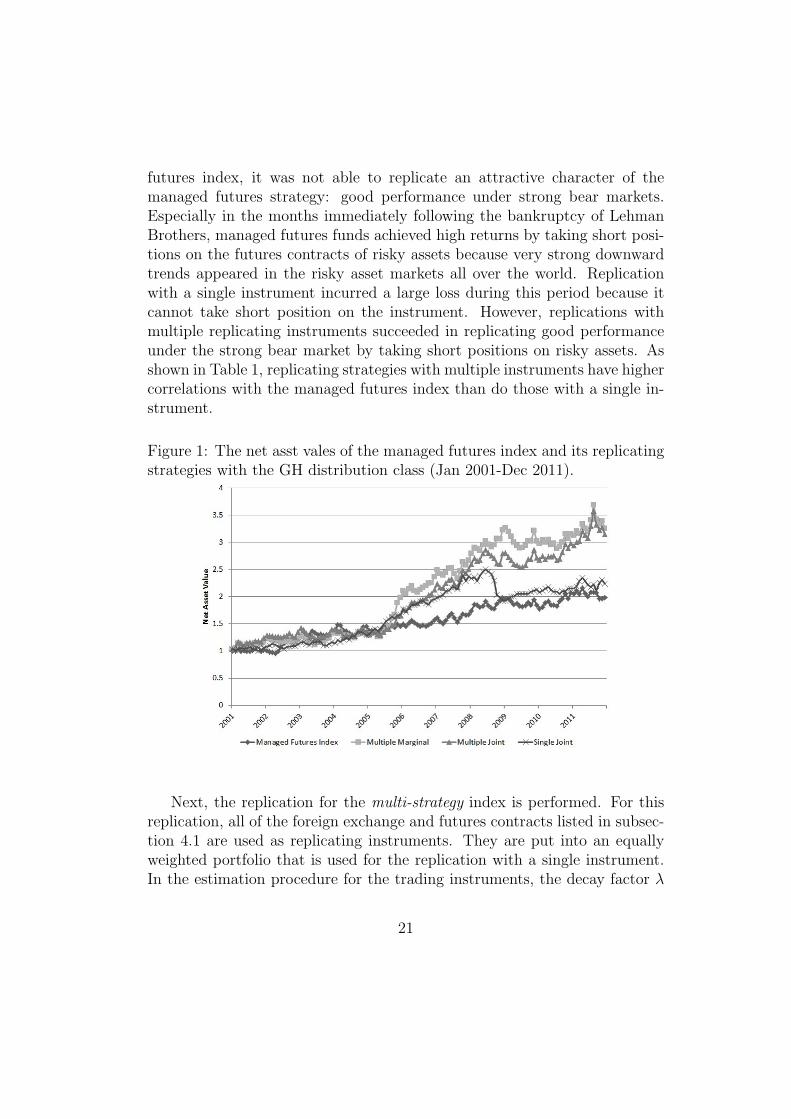
futures index, it was not able to replicate an attractive character of themanaged futures strategy: good performance under strong bear markets.Especially in the months immediately following the bankruptcy of LehmanBrothers, managed futures funds achieved high returns by taking short posi-tions on the futures contracts of risky assets because very strong downwardtrends appeared in the risky asset markets all over the world. Replicationwith a single instrument incurred a large loss during this period because itcannot take short position on the instrument. However, replications withmultiple replicating instruments succeeded in replicating good performanceunder the strong bear market by taking short positions on risky assets. Asshown in Table 1, replicating strategies with multiple instruments have highercorrelations with the managed futures index than do those with a single in-strument.

Figure 1: The net asst vales of the managed futures index and its replicatingstrategies with the GH distribution class (Jan 2001-Dec 2011).

Next, the replication for the multi-strategy index is performed. For thisreplication, all of the foreign exchange and futures contracts listed in subsec-tion 4.1 are used as replicating instruments. They are put into an equallyweighted portfolio that is used for the replication with a single instrument.In the estimation procedure for the trading instruments, the decay factor λ

21

is assumed to be 0.9975. Other procedures are the same as in the replica-tions for the managed futures. Table 2 shows the summary statistics of thereplication results. The replications with the GH distribution class obtainedhigher mean returns than did those with GM distributions for this case, aswell.

Table 2: Summary Statistics on the Log Returns of the Multi-Strategy Indexand Its Replicating Strategies (2001-2011)

Multi-Strategy Multiple Multiple SingleIndex Marginal Joint Joint

Mean 0.52％ 0.49％ 0.55％ 0.30％Std. Dev. 1.62％ 1.94％ 1.72％ 1.16％

Mean/Std. Dev 0.32 0.25 0.32 0.26Skew -2.03 -0.28 0.37 -0.75

Kurtosis 11.21 6.70 5.64 5.30Max 4.19％ 7.74％ 7.41％ 2.98％Min -7.63％ -7.55％ -4.20％ -4.56％

Correlation with0.54 0.15 0.16 0.55



(a) Generalized Hyperbolic Class

Multi-Strategy Multiple Multiple SingleIndex Marginal Joint Joint

Mean 0.52％ 0.37％ 0.41％ 0.27％Std. Dev. 1.62％ 1.85％ 1.63％ 1.39％

Mean/Std. Dev 0.32 0.20 0.25 0.20Skew -2.03 -2.02 -2.25 -3.91

Kurtosis 11.21 9.50 12.11 31.62Max 4.19％ 4.03％ 3.71％ 2.92％Min -7.63％ -8.58％ -8.80％ -10.65％




(b) Gaussian Mixture Distributions

Figure 2 shows the net asset values of the multi-strategy index and repli-cating strategies with the GH distribution class. The replication for the joint

22

distribution with multiple assets outperformed the multi-strategy index. Thereplication for the marginal distribution slightly underperformed the multi-strategy index, but it attained a close return level. The extension to multipleassets much improved the performance for this case, as well.

Figure 2: The net asst vales of the multi-strategy index and its replicatingstrategies with the GH distribution class (Jan 2001-Dec 2011).

Finally, let us replicate the global macro index. In this replication, theentire procedure is exactly the same as it was in the replication for the multi-strategy case. Table 3 shows the summary statistics of the replication results.The replications with the GH distribution class attained higher mean returnsthan did those with GM distributions for the global macro case, as well. Thisphenomenon is observed for all of the replications for the three strategies.

Figure 3 shows the net asset values of the global macro index and thereplicating strategies for the GH distribution class. Replicating strategiescould not attain returns that were as high as those of the global macroindex. The following two reasons for this failure are considered. First, thereturn distribution of the global macro index changes substantially with time.Therefore, it is difficult to replicate it on an out-of-sample basis. Second, theperformance of the global macro index during the sample period is very high.As previously mentioned, the performance of the global macro index from

23

Table 3: Summary Statistics on the Log Returns of the Global Macro Indexand Its Replicating Strategies (2001-2011)

Global Macro Multiple Multiple SingleIndex Marginal Joint Joint

Mean 0.89％ 0.63％ 0.74％ 0.42％Std. Dev. 1.51％ 2.79％ 2.71％ 2.02％

Mean/Std. Dev 0.59 0.23 0.27 0.21Skew -1.41 -0.37 0.03 -0.31

Kurtosis 9.21 5.66 5.49 7.63Max 4.35％ 10.20％ 10.46％ 7.81％Min -6.86％ -9.37％ -8.63％ -8.99％




(a) The Generalized Hyperbolic Class

Global Macro Multiple Multiple SingleIndex Marginal Joint Joint

Mean 0.89％ 0.55％ 0.57％ 0.44％Std. Dev. 1.51％ 2.83％ 2.86％ 2.07％

Mean/Std. Dev 0.59 0.19 0.20 0.21Skew -1.41 -1.00 -0.93 -1.68

Kurtosis 9.21 7.47 7.82 16.96Max 4.35％ 10.20％ 10.46％ 7.81％Min -6.86％ -11.07％ -10.87％ -12.96％




(b) Gaussian Mixture Distributions

24

2001 to 2011 is the best among the Dow Jones Credit Suisse Hedge FundIndices. Although replicating strategies with multiple instruments underper-formed the global macro index, the extension to multiple assets improves theperformance substantially.

Figure 3: The net asst vales of the global macro index and its replicatingstrategies with the GH distribution class (Jan 2001-Dec 2011).

5 Conclusion

This article presented a new method to construct the cheapest dynamicportfolio that generates a target payoff distribution or its joint distributionwith the investor’s existing portfolio. It was shown that the cost minimiza-tion is equivalent to the maximization of a certain class of von Neumann-Morgenstern utility functions. This method is regarded as an extension ofthe hedge fund replication methods that were developed by Kat and Palaro(2005a, b) and Papageorgiou, Remillard and Hocquard (2008). Their meth-ods replicate the distribution of the target hedge fund and its dependenceupon the investor’s existing portfolio by trading the investor’s portfolio andone replicating instrument with only long positions. Our method extends

25

their approach to allow for the trading of multiple assets with both long andshort positions.

Finally, the method was applied to the replications of three hedge fundstrategies: managed futures, multi-strategy and global macro. The replica-tion performances were examined on an out-of-sample basis. The resultsshowed that the performances of the replications improved substantially ascompared to the case of one replicating instrument with only long positions.Additionally, two different distribution classes, the Generalized Hyperbolic(GH) distribution class and Gaussian Mixture (GM) distributions, are ap-plied to the estimation of the target hedge fund indices’ returns; replicationswith the GH distribution class outperformed those with the GM distributionfor all of the three strategies. As a next research topic, the implementation ofthe Markovian coefficients case, including a stochastic volatility model and astochastic interest rate model, is a challenging task. Additionally, the appli-cations of our method to creating attractive new trading strategies and riskmanagement are interesting topics.

26

Tab

le4:

SummaryStatisticsof

Mon

thly

Log

Returnsof

Dow

Jon

esCreditSuisse

Hedge

FundIndexes

All

Convertible

Ded

icated

Emerging

Equity

Even

tFixed

Inco

me

Global

Long/Short

Managed

Multi

Strategies

Arb

itrage

Short

Bias

Markets

Market

Neu

tral

Driven

Arb

itrage

Macro

Equity

Futu

res

Strategy

Mea

n0.76％

0.68％

-0.37％

0.57％

0.45％

0.77％

0.45％

1.04％

0.82％

0.46％

0.67％

Std

.Dev

.2.19％

2.09％

4.92％

4.24％

3.84％

1.89％

1.76％

2.79％

2.89％

3.46％

1.50％

Mea

n/Std

.Dev

0.35

0.32

-0.08

0.13

0.12

0.41

0.25

0.37

0.28

0.13

0.45

Skew

-0.34

-3.16

0.49

-1.61

-12.56

-2.59

-4.77

-0.25

-0.27

-0.06

-2.04

Kurtosis

5.74

22.22

3.80

11.15

174.27

15.89

37.17

7.35

6.39

2.90

11.44

Max

8.18％

5.65％

20.47％

14.27％

3.59％

4.13％

4.24％

10.07％

12.23％

9.49％

4.19％

Min

-7.85％

-13.46％

-11.97％

-26.17％

-51.84％

-12.53％

-15.12％

-12.27％

-12.14％

-9.82％

-7.63％

(a)Total

Period:19

95-2011

All

Convertible

Ded

icated

Emerging

Equity

Even

tFixed

Inco

me

Global

Long/Short

Managed

Multi

Strategies

Arb

itrage

Short

Bias

Markets

Market

Neu

tral

Driven

Arb

itrage

Macro

Equity

Futu

res

Strategy

Mea

n1.22％

0.81％

-0.22％

0.86％

0.87％

0.96％

0.53％

1.14％

1.03％

0.58％

0.83％

Std

.Dev

.2.90％

1.34％

5.01％

4.41％

0.77％

1.69％

1.09％

3.06％

2.98％

3.37％

1.04％

Mea

n/Std

.Dev

0.42

0.60

-0.04

0.19

1.12

0.57

0.49

0.37

0.35

0.17

0.80

Skew

-0.26

-1.66

0.67

-1.80

0.38

-4.12

-3.54

-0.39

-0.07

0.01

-1.31

Kurtosis

3.79

11.81

4.42

7.52

3.33

31.83

22.39

3.81

5.52

3.99

9.22

Max

8.18％

3.51％

20.47％

14.27％

3.21％

3.52％

2.03％

9.95％

12.23％

9.49％

3.08％

Min

-7.85％

-4.79％

-9.09％

-26.17％

-1.15％

-12.53％

-7.22％

-12.27％

-12.14％

-9.02％

-4.87％

(b)Former

Sub-period:19

95-2000

All

Convertible

Ded

icated

Emerging

Equity

Even

tFixed

Inco

me

Global

Long/Short

Managed

Multi

Strategies

Arb

itrage

Short

Bias

Markets

Market

Neu

tral

Driven

Arb

itrage

Macro

Equity

Futu

res

Strategy

Mea

n0.51％

0.45％

-0.43％

0.73％

0.08％

0.60％

0.36％

0.89％

0.41％

0.52％

0.52％

Std

.Dev

.1.63％

2.36％

4.49％

2.97％

4.69％

1.80％

1.96％

1.51％

2.21％

3.45％

1.62％

Mea

n/Std

.Dev

0.31

0.19

-0.10

0.25

0.02

0.34

0.18

0.59

0.19

0.15

0.32

Skew

-1.51

-2.96

0.07

-1.57

-10.49

-1.36

-4.68

-1.41

-0.90

-0.15

-2.03

Kurtosis

7.80

19.60

2.61

8.43

119.57

5.58

34.77

9.21

4.90

2.37

11.21

Max

3.98％

5.65％

9.81％

6.72％

3.59％

4.13％

4.24％

4.35％

5.10％

8.28％

4.19％

Min

-6.78％

-13.46％

-11.97％

-14.65％

-51.84％

-5.92％

-15.12％

-6.86％

-8.14％

-9.02％

-7.63％

(c)LatterSub-period:20

01-2011

27

Tab

le5:

SummaryStatisticsof

theInvestor’sPortfolio

andReplicatingInstruments

investor’s

long-term

TOPIX

USD

EUR

GBP

CHF

AUD

Gold

US10yr

S＆

PW

TI

portfolio

JGB

/JPY

/JPY

/JPY

/JPY

/JPY

/JPY

/JPY

T-N

ote

500

crudeoil

Mea

n0.03％

0.20％

-0.29％

-0.11％

0.15％

0.03％

0.20％

0.59％

1.02％

0.34％

-0.19％

0.62％

Std

.Dev

.2.45％

0.87％

5.24％

2.74％

3.55％

3.57％

3.30％

4.53％

5.09％

2.69％

5.81％

10.16％

Mea

n/Std

.Dev

.0.01

0.24

-0.05

-0.04

0.04

0.01

0.06

0.13

0.20

0.13

-0.03

0.06

(a)Meanan

dStandardDeviation

investor’s

long-term

TOPIX

USD

EUR

GBP

CHF

AUD

Gold

US10yr

S＆

PW

TI

portfolio

JGB

/JPY

/JPY

/JPY

/JPY

/JPY

/JPY

/JPY

T-N

ote

500

crudeoil

investor’sportfolio

1.00

-0.17

0.99

0.31

0.41

0.38

0.30

0.58

0.22

0.13

0.65

0.38

long-term

JGB

-0.17

1.00

-0.32

-0.14

0.00

-0.13

0.04

-0.13

-0.09

0.10

-0.16

-0.15

TOPIX

0.99

-0.32

1.00

0.32

0.40

0.40

0.29

0.59

0.24

0.12

0.66

0.40

USD/JPY

0.31

-0.14

0.32

1.00

0.51

0.67

0.39

0.47

0.27

0.75

0.56

0.40

EUR/JPY

0.41

0.00

0.40

0.51

1.00

0.76

0.85

0.81

0.44

0.44

0.58

0.53

GBP/JPY

0.38

-0.13

0.40

0.67

0.76

1.00

0.63

0.70

0.41

0.47

0.55

0.61

CHF/JPY

0.30

0.04

0.29

0.39

0.85

0.63

1.00

0.68

0.41

0.34

0.40

0.44

AUD/JPY

0.58

-0.13

0.59

0.47

0.81

0.70

0.68

1.00

0.47

0.32

0.74

0.63

Gold

0.22

-0.09

0.24

0.27

0.44

0.41

0.41

0.47

1.00

0.29

0.23

0.38

US10yrT-N

ote

0.13

0.10

0.12

0.75

0.44

0.47

0.34

0.32

0.29

1.00

0.24

0.21

S＆

P500

0.65

-0.16

0.66

0.56

0.58

0.55

0.40

0.74

0.23

0.24

1.00

0.44

WTIcrudeoil

0.38

-0.15

0.40

0.40

0.53

0.61

0.44

0.63

0.38

0.21

0.44

1.00

(b)Correlation

Matrix

28

References

Agarwal, V. and N.Y. Naik (2004). Risks and Portfolio Decisions InvolvingHedge Funds. The Review of Financial Studies, Vol. 17(1), pp. 63-98.

Amin, G. and H.M. Kat (2003). Hedge Fund Performance 1990-2000: Do theMoney Machines Really Add Value? Journal of Financial and QuantitativeAnalysis, Vol. 38(2), pp. 251-274.

Cvitanic, V. Polimenis and F. Zapatero (2008). Optimal Portfolio Allocationwith Higher Moments. Annals of Finance, Vol. 4, pp. 1-28.

Duarte, J., F. Longstaff, and F. Yu (2007). Risk and Return in Fixed In-come Arbitrage: Nickels in front of a Steamroller? The Review of FinancialStudies, Vol. 20(3), pp. 769-811.

Dybvig, P. (1988a). Distributional Analysis of Portfolio Choice. Journal ofBusiness, Vol. 61, pp. 369-393.

Dybvig, P. (1988b). Inefficient Dynamic Portfolio Strategies or How toThrow Away a Million Dollars in the Stock Market. The Review of Fi-nancial Studies, Vol. 1, pp. 67-88.

Fung, W. and D.A. Hsieh (1997). Empirical Characteristics of DynamicTrading Strategies: The Case of Hedge Funds. The Review of FinancialStudies, Vol. 10(2), pp. 275-302.

Fung, W. and D.A. Hsieh (2000). Performance Characteristics of HedgeFunds and Commodity Funds: Natural vs. Spurious Biases. The Journal ofFinancial and Quantitative Analysis, Vol. 35(3), pp. 291-307.

Fung, W. and D.A. Hsieh (2001). The Risk in Hedge Fund Strategies: The-ory and Evidence from Trend Followers. The Review of Financial Studies,Vol. 14(2), pp. 313-341.

Fung, W. and D.A. Hsieh (2007a). Will Hedge Funds Regress towards Index-like Products? Journal of Investment Management, Vol. 5(2), pp. 46-55.

Fung, W. and D.A. Hsieh (2007b). Hedge Fund Replication Strategies: Im-plications for Investors and Regulators. Banque de France, Financial Sta-bility Review, Special issue on hedge funds, Vol. 10 April, pp. 55-66.

29

Hakamada, T., A. Takahashi, and K. Yamamoto (2007). Selection and Per-formance Analysis of Asia-Pacific Hedge Funds. The Journal of AlternativeInvestments, Vol. 10(3), pp. 7-29.

Hellmich, M. and S. Kassberger (2011). Efficient portfolio optimization themultivariate Generalized Hyperbolic framework. Quantitative Finance, Vol.11(10), pp. 1503-1516.

Hocquard, A., N. Papageorgiou, and B. Remillard (2012) The Payoff Distri-bution Model: An Application to Portfolio Insurance Quantitative Finance,Forthcoming.

Joe, H. (1997). Multivariate Models and Dependence Concepts. Chapmanand Hall.

Karatzas, I. and S. Shreve (1998). Methods of Mathematical Finance.Springer.

Kat, H.M. and H.P. Palaro (2005a). Who Needs Hedge Funds? A Copula-Based Approach to Hedge Fund Return Replication. Working Paper.

Kat, H.M. and H.P. Palaro (2005b). Hedge Fund Returns: You Can MakeThem Yourself! Journal of Wealth Management, Vol. 8(2), pp. 62-68.

Lo, A. and J. Hasanhodzic (2007). Can Hedge-Fund Returns Be Replicated?:The Linear Case. Journal of Investment Management, Vol. 5(2), pp. 5-45.

Malkiel, B.G. and A. Saha (2005). Hedge Funds: Risk and Return. TheFinancial Analysts Journal, Vol. 61(6), pp. 80-88.

Markowitz, H.M. (1952). Portfolio Selection. The Journal of Finance, Vol.7(1): pp. 77-91

McNeil, A.J., R. Frey and P. Embrechts (2005). Quantitative Risk Manage-ment: Concepts, Techniques, and Tools. Princeton University Press.

Merton, R.C. (1969). Lifetime Portfolio Selection under Uncertainty: Thecontinuous time case. Review of Economics & Statistics, Vol. 51(3), pp.247-257

Merton, R.C., (1971). Optimum Consumption and Portfolio Rules in aContinuous-time Model, Journal of Economic Theory, Vol. 3(4), pp. 373-413

30

Mitchell, M. and T. Pulvino (2001). Characteristics of Risk in Risk Arbi-trage. Journal of Finance, Vol. 56, pp. 2067-2109.

Nelsen, R.B. (1999). An introduction to copulas: Vol. 139 of Lecture Notesin Statistics. Springer-Verlag, New York.

Nualart, D. (2006). The Malliavin Calculus and Related Topics 2nd Edition,Springer.

Ocone, D., and I. Karatzas (1991). A Generalized Clark RepresentationFormula, with Applications to Optimal Portfolios. Stochastics, Vol. 37, pp.187-220.

Papageorgiou, N., B. Remillard, and A. Hocquard (2008). Replicating theProperties of Hedge Fund Returns. The Journal of Alternative Investments,Vol. 11(2), pp. 8-38.

Takahashi, A., and K. Yamamoto (2010). Hedge Fund Replication. Chapter2 in The Recent Trend of Hedge Fund Strategies, Nova Science Publishers,pp. 57-95.

Takahashi, A., and K. Yamamoto (2010). A New Hedge Fund ReplicationMethod with the Dynamic Optimal Portfolio. Global Journal of BusinessResearch, Vol. 4(4), pp. 23-34.

Takahashi, A., and N. Yoshida (2004). An Asymptotic Expansion Schemefor Optimal Investment Problems. Statistical Inference for Stochastic Pro-cess, Vol. 7, pp. 153-188.

Tuchschmid, N.S., E. Wallerstein and S. Zaker (2010). How Do Hedge FundClones Manage the Real World? The Journal of Alternative Investments,Vol. 12(3), pp. 37-50.

Tuchschmid, N.S., E. Wallerstein and S. Zaker (2012). Hedge Fund Clones,Chapter 8 in The Oxford Handbook of Quantitative Asset Management, Ox-ford University Press, pp. 136-153.

31

6 Appendix

6.1 Proof of Theorem 1

First, let us show that the cheapest way to obtain a target distribution isachieved by allocating the terminal wealth in the reverse order of the stateprice density. The reverse order of the state price density is mathematicallydefined as follows. Let Z be a random variable. For ω∗ ∈ Ω, define UZ(ω

∗)as

UZ(ω∗) = ω : HT (ω) < HT (ω

∗) ∩ ω : Z(ω) < Z(ω∗),

and letVZ = ∪ω∗∈ΩUZ(ω

∗).

Z is the reverse order of the state price density if

P(VZ) = 0.

Assume that the FT -measurable random variable Z has the same distributionas ξ, and is not the reverse order of the state price density. Then, there exista−1 < a+1 ≤ a−2 < a+2 , such that

HT (ω1) < HT (ω2) for any (ω1, ω2) ∈ A1 × A2, (12)

where A1 = a−1 < Z < a+1 , A2 = a−2 < Z < a+2 , and P(A1) = P(A2) > 0.Z is not the reverse order of HT on A1 ∪ A2.

The following discussion shows that a payoff cheaper than Z can be cre-ated without changing the distribution by switching the values on A1 andA2. Let p

±i = P(Z ≤ a±i ), I1 = (p−1 , p

+1 ], and I2 = (p−2 , p

+2 ]. Define Z

′ as

Z ′ = G(Fξ(Z)),

where function G is defined as

G(p) =

F−1ξ (p) on (0, 1) \ (I1 ∪ I2),F−1ξ (p+ p−2 − p−1 ) on I1,

F−1ξ (p+ p−1 − p−2 ) on I2.

Here, note that p+1 − p−1 = p+2 − p−2 . Then, Z′ has the same distribution as ξ

because the equationP(Z ′ ≤ a) = Fξ(a) (13)

32

holds true for any a > 0, as shown in the following. For 0 < a ≤ a−1 ,

P(Z ′ ≤ a) = Fξ(a).

For a ∈ (a−1 , a+1 ],

P(Z ′ ≤ a) = P(Z ′ ≤ a−1 ) + P(a−1 < Z ′ ≤ a)

= P(Z ≤ a−1 ) + P(a−1 < G(Fξ(Z)) ≤ a)

= p−1 + P(Fξ(a−1 ) < Fξ(Z) + p−2 − p−1 ≤ Fξ(a))

= Fξ(a).

The same arguments prove that equation (13) holds true for any a in theother intervals.

The difference in the costs is given by

E[HTZ]− E[HTZ′] = E[HT (Z − Z ′)1A2 ]− E[HT (Z

′ − Z)1A1 ].

As Z ′ is created by switching the values of Z ′ on A1 and A2, (Z−Z ′)1A2 and(Z ′ − Z)1A1 have the same distribution. Noting inequality (12),

E[HTZ]− E[HTZ′] > 0.

To summarize, Z ′ has the same distribution as ξ with a cheaper cost thanZ. Therefore, to obtain the same distribution as ξ at time T , the terminalwealth should be in the reverse order of the state price density. Because X isthe reverse order of HT , X is one of the cheapest payoffs that has the samedistribution as ξ.

Next, let us prove the uniqueness. Let X ′ be a random variable that hasthe same distribution as ξ, and is the reverse order of HT . Then, P (VX′) = 0.For any ω∗ ∈ Ω \ VX′ ,

Pω : LT (ω) ≤ LT (ω∗) = Pω : X ′(ω) ≤ X ′(ω∗).

Therefore,FLT

(LT (ω∗)) = Fξ(X

′(ω∗)).

By operating F−1ξ to the both sides of the equation,

F−1ξ (FLT

(LT (ω∗))) = X ′(ω∗).

Hence, X ′ = X. 2

33


Let x be the initial cost for the payoff X (i.e., x = E[HTX]). As X is definedby equation (5), HT = exp[−f−1(X)]. exp[−f−1(·)] is a positive, strictlydecreasing function. Define u(·) as

u(z) = λ

∫ z

0

exp[−f−1(ζ)]dζ,

where λ is a positive number. Then, u(·) is strictly increasing and strictlyconcave. It is also true that limz→+0 u

′(z) = +∞ and limz→+∞ u′(z) = 0.Moreover, u′(X) = λHT . This is the first order condition of the optimalityfor von Neumann-Morgenstern utility u(·) (see, for example, Karatzas andShreve (1998)). The budget constraint x = E[HTu

′−1(λHT )] is also satisfied.Conversely, assume a dynamic trading strategy with the initial cost x′,

generating payoff the X ′ maximizes a strictly increasing and strictly con-cave von Neumann-Morgenstern utility u(·) satisfying conditions (a) and (b).Then, u′(X ′) = λ′HT is satisfied for some λ′ > 0. Therefore, X ′ is the re-verse order of HT . According to the argument in the proof of Theorem 1,this strategy attains the cheapest payoff among the random variables whosedistribution is the same as X ′. 2


The basic idea is the same as the proof of theorem 1. Let Z be a randomvariable whose joint distributions with S1

T is the same as (S1T , ξ). Define

SZ ⊂ R+ and B1Z ⊂ Ω as

SZ = s : Z is not reverse order of HT under the condition S1T = s,

B1Z = ω : S1

T (ω) ∈ SZ.Assume that P(B1

Z) > 0. For any s ∈ SZ , there exist as−1 < as+1 ≤ as−2 < as+2 ,

such thatHT (ω1) < HT (ω2) for any (ω1, ω2) ∈ As

1 × As2, (14)

where As1 = S1

T = s, as−1 < Z < as+1 , As2 = S1

T = s, as−2 < Z < as+2 ,and P(As

1|S1T = s) = P(As

2|S1T = s) > 0. Let ps±i = P(Z ≤ as±i |S1

T = s),Is1 = (ps−1 , ps+1 ] and Is2 = (ps−2 , ps+2 ]. Introduce random variable Z ′, defined by

Z ′ =

G1(S1

T , Fξ|S1T(Z)) on B1

Z ,

Z on Ω \B1Z ,

34

where G1 is defined as

G1(s, p) =

F−1ξ|s (p) for p ∈ (0, 1) \ (Is1 ∪ Is2),F−1ξ|s (p+ ps−2 − ps−1 ) for p ∈ Is1 ,

F−1ξ|s (p+ ps−1 − ps−2 ) for p ∈ Is2 .

Here, note that ps+1 − ps−1 = ps+2 − ps−2 . Then, (S1T , Z

′) has the same distri-bution as (S1

T , Z), and Z′ is cheaper than Z because of the same argument

in the proof of Theorem 1. Therefore, to obtain the cheapest payoff whosejoint distribution with S1

T is the same as (S1T , ξ), the terminal wealth should

be the reverse order of HT under the condition that S1T is known. Therefore,

the X defined by equation (6) is the cheapest payoff.Next, let us prove the uniqueness. Suppose that X ′ is a random variable

whose joint distribution with S1T is the same as (S1

T , ξ) and is the reverseorder of HT under the condition that S1

T is known. Then, P(B1X′) = 0. For

s ∈ R+ \ SZ and ω∗ ∈ S1T = s, define U s

X′(ω∗) as

U sX′(ω∗) = ω : ST (ω) = s,HT (ω) < HT (ω

∗), and X ′(ω) < X ′(ω∗),

and letV sX′ = ∪ω∗∈S1

T=sUsX′(ω∗),

CX′ = (Ω \B1X′) \ (∪s∈SX′V

sX′).

Then, P(V sX′|S1

T = s) = 0. Because it is satisfied that

P(∪s∈SX′VsX′) =

∫SX′

P(V sX′|S1

T = s)FS1T(ds) = 0,

P(CX′) = 1. For any s ∈ R+ \ SZ and ω∗ ∈ CX′ ,

Pω : LT (ω) ≤ LT (ω∗)|S1

T = s = Pω : X ′(ω) ≤ X ′(ω∗)|S1T = s.

Therefore,FLT |s(LT (ω

∗)) = Fξ|s(X′(ω∗)).

By operating F−1ξ|s to both of the sides of the equation,

F−1ξ|s (FLT |s(LT (ω

∗))) = X ′(ω∗).

Hence, X ′ = X. 2

35

6.4 Derivation of the Dynamic Replicating Portfolios

For the case of the Markovian coefficients, the concrete expressions for thecheapest dynamic portfolios can be obtained.2 Suppose that a k-dimensionalstate variable Yt follows SDE

dYt = µY (Yt)dt+ σY (Yt)dWt (15)

and rt, µt, and σt can be described by differentiable functions of state variableYt: rt = r(Yt), µt = µ(Yt), and σt = σ(Yt). The following proposition givesthe dynamic portfolios that generates the payoffs.

Proposition 2 Assume that r, µ and σ are functions of Yt following SDE(15). Then, in a complete market M, the dynamic portfolio that generatespayoff f(LT ) is given by

πMt = σ′(t)−1ϕM

t , (16)

where

ϕMt = Xtθt +

1

Ht

E[HTf ′(LT )−XTDLT|Ft]. (17)

DLTis given by

DLT=

∫ T

t

∂r(Ys)At,sσY (Yt)ds+

∫ T

t

n∑j=1

θj(Ys)∂θj(Ys)At,sσ

Y (Yt)ds

+

∫ T

t

n∑j=1

∂θ(Ys)At,sσY (Yt)dW

js + θ(Yt)

′,

where At,s is a k × k-valued unique solution of the SDE

dAt,s =n∑

i=1

∂σYi (Ys)At,sdW

is

with an initial condition At,t = I. σYi (·) and I denotes the i-th row of the

matrix σY (·) and the k × k identity matrix, respectively.

2The martingale method with Malliavin calculus easily gives us the dynamic portfoliothat generate the payoffs. See, for example, Karatzas and Shreve (1998) for the basics ofthe martingale method and Nualart (2006) for the introduction to Malliavin calculus. Asfor the application of Malliavin calculus to the dynamic optimal portfolio and its closedform evaluation, see, for example, Ocone and Karatzas (1991) and Takahashi and Yoshida(2004).

36

The portfolio that attains payoff g(S1T , LT ) is given by

πJt = σ′(t)−1ϕJ

t , (18)

where

ϕJt = Xtθt +

1

Ht

E[HTg1(S1T , LT )DS1

T+HTg2(S1

T , LT )−XTDLT|Ft]. (19)

gi (i = 1, 2) represents the partial derivative of g with respect to the i-thargument. DS1

Tis given by

DS1T= S1

T

∫ T

t

∂µ1(Ys)− σ11(Ys)∂σ11(Yu)At,sσ

Y (Yt)ds

+ S1T

∫ T

t

∂σ11(Ys)At,sσY (Yt)dW

1s

+ (S1Tσ

11(Yt), 0, · · · , 0).

Proof. By the argument in Karatzas and Shreve (1998), πt is described as

πt = σ′t−1

(Xtθt +

ψt

Ht

), (20)

where ψt is given by the following martingale representation

Mt = E[HTXT |Ft] = x+

∫ t

0

ψ′udWu.

Applying the Clark-Ocone formula (see, for example, pp. 46 in Nualart(2006)), ψt is given by

ψt = E[Dtη|Ft], (21)

where η = HTXT , and Dt denotes the Malliavin derivative: Dtη =(D1tη, · · · ,Dntη).

To generate the marginal payoff distribution, XT = f(LT ). Then, Dtηcan be calculated as

Dtη = (DtHT )XT +HTf′(LT )DtLT . (22)

To generate the joint distribution with the investor’s portfolio, XT =g(S1

T , LT ). Then, Dtη can be calculated as

Dtη = (DtHT )XT +HTg1(S1T , LT )DtS

1T +HTg2(S

1T , LT )DtLT , (23)

37

where gi (i = 1, 2) represents the partial derivative of g with respect to thei-th argument.

DtHT , DtLT and DtS1T are calculated as

DtHT = −HTDtLT ,

DtLT =

∫ T

t

∂r(Ys)DtYsds+

∫ T

t

n∑j=1

θj(Ys)∂θj(Ys)DtYsds

+

∫ T

t

n∑j=1

∂θ(Ys)DtYsdWjs + θ(Yt)

′,

DtS1T = S1

T

∫ T

t

∂µ1(Ys)− σ11(Ys)∂σ11(Yu)DtYsds

+ S1T

∫ T

t

∂σ11(Ys)DtYsdW1s

+ (S1Tσ

11(Yt), 0, · · · , 0).

In this case, DtYs can be calculated concretely. Let At,s be a k × k-valuedunique solution of the SDE

dAt,s =n∑

i=1

∂σYi (Ys)At,sdW

is

with the initial condition At,t = I, where σYi (·) denotes the i-th row of matrix

σY (·), and I is the k × k identity matrix. DtYs is represented as

DtYs = At,sσY (Yt) (24)

(see, for example, pp. 126 in Nualart (2006)). Therefore, the proposition isobtained. 2

Proposition 1 in the main text can be directly derived from this proposi-tion.

38

Documents

CIRJE-F-624 Generating a Target Payoff Distribution with