Chem 406 - Lecture 7 · Chem 406 - Lecture 7 ... Louis de Broglie ... calc = ()xyz ei2 ()hx +ky lz z y x Model Building A model is fit to the electron density: 57

Chem 406 - Lecture 7

Structure Determination by X’Ray Crystallography

Introduction

• Earlier in the semester we developed a crude model for

macromolecules using sedimentation analysis.

Prolate and oblate ellipsoids of revolution

2

Introduction

• Since the late 1950’s we have had models with atomic resolution.

3

Protein Data Bank

4

Protein Data Bank

5

Protein Data Bank

6

Electromagnetic Radiation

7

Snell’s Law

8

n1 sin 1( ) = n2 sin 2( )

n1

n2

Lenses

9

Microscopy

Light microscopy

10

Electromagnetic

Spectrum

11

H2O

glucose

lipids

proteins

ribosomes

viruses

mitochondriabacteria

eukaryoticcells

To use electromagnetic radiation to create images of objects requires electromagnetic radiation having wavelengths that are equal to or small than the objects being imaged.

footballfield

house

human

baseball

Louis de Broglie

In 1924 proposed

• Just as light has a particle-like nature

• Matter has a wave-like nature

12

E = h

=h

p

=h

mv

Planck

de Broglie

High Energy Electron Beam

• For a 100 kV beam, in which an electron is accelerated through a 100,000 V potential field.

13

=h

mv= 0.004 nm

= 0.04 Å

Microscopy

Comparing light microscopy to electron microscopy

14

{

X-ray Crystallography

The Crystal Lattice

15

Unit Cell


The Unit Cell

16


The Bravais Lattice Types

17


Protein Crystals

18


Protein Crystals

19


Growing Crystals

20


Growing Crystals

21


Growing Crystals

22


Diffraction from Crystals

23


Diffraction fromCrystals

24


25

In light microscoscopy, lenses are used to collect the light scattered from an object and use it to form an image.


26

There are no X-ray lenses

• Computers are used to simulate a lens

• To understand how this works, we need to understand the elements of a diffraction pattern

The Diffraction Pattern

Constructive and Destructive Interference

27

ConstructiveInterference

DestructiveInterference


Bragg’s Law describes the conditions required for obtaining a spot.

• Constructive interference occurs when

- William Henry Bragg, and his son William Lawrence Bragg, shared the Nobel Prize in Physics in 1915.

28

d sin( )

2d sin( ) = n (Bragg’s Law)


Crystal Diffraction

• The spots arise from reflections off of the crystal planes

29


Crystal Diffraction

30


The spots in the diffraction pattern arise from constructive and destructive interference between x-rays scattered from the different planes in the unit cell

• The spacings and angles arise from the unit cell dimensions and angles (a, b, c, , & )

31


Demos

• XRayView 3.0- Simulates diffraction from a crystal

• Optical Diffraction- Diffraction patterns are reciprocally related to the object responsible for the

diffraction

32


The diffraction pattern is also referred to at the reciprocal lattice.

33

The Fourier Series

Fourier Series

• Sine and Cosine waves have- Amplitude, F

- Frequency, h

- Phase,

34

f x( ) = Fo cos 2 hx +[ ]( )

f x( ) = Fo sin 2 hx +[ ]( )

or

The Fourier Series

Fourier Synthesis- Approximating a square wave

by a Fourier Series

35

f x( ) = Fo cos 2 0x + o[ ]( )

+F1 cos 2 1x + 1[ ]( )

+F2 cos 2 2x + 2[ ]( )

+F3 cos 2 3x + 3[ ]( )...

+Fn cos 2 nx + n[ ]( )

= Fh cos 2 hx + h[ ]( )h=0

n

Fourier Series

An alternative to designating a phase angle, , is to combine cosine and sine wave

• The sine is equal to a cosine which has been shifted by an angle of /2 (90°)

• This allows us to replace

36

sin x( ) = cos x + 2( )

f x( ) = Fh cos 2 hx + h[ ]( )h=0

n

with

f x( ) = Fh,cos cos 2 hx( ) + Fh,sin sin 2 hx( )( )h=0

n

Fourier Series

It is also mathematically convenient to represent this relationship using complex numbers.

• The cosine portion represents the Real part, while the sine portion represents the Imaginary part,of the complex number

37

f x( ) = Fh cos 2 hx( ) + i sin 2 hx( )( )h=0

n

x = a + ib, where i = 1

where the amplitude, Fh , is also a complex number

Fourier Series

Another mathematical convenience comes from making use of Euler’s formula:

• This allows us to cast the Fourier series into a nice, compact, complex exponential form:

38

cos x( ) + i sin x( ) = eix

f x( ) = Fhei2 hx

h=0

n

Fourier Series

The complex polar coordinate system

39

Applying the Fourier Series to Diffraction

• The diffraction pattern also called the reciprocal lattice.

• Each spot in the diffraction pattern is called a structure factor

- The structure factors are represented in three dimensions by the symbol

- Where h, k, and l are the Miller indices, which describe the sets of planes that can be used to divide up the unit cell in the crystal lattice.

40

Fh,k ,l


• The diffraction pattern also called the reciprocal lattice.

• Each spot in the diffraction pattern is called a structure factor

- The structure factors are represented in three dimensions by the symbol

- Where h, k, and l are the Miller indices, which describe the sets of planes that can be used to divide up the unit cell in the crystal lattice.

Remember, According to Bragg’s Law, it is the reflections from these planes that

give rise to the diffraction pattern.

41

Fh,k ,l


Crystal Diffraction

42


The diffraction pattern is also referred to at the reciprocal lattice.

43

44


The structure factors (spots), Fh,k,l

45

Fhkl = fA + fB + ...+ fA ' + fB ' + ...+ fF 'Sum over

atoms

The structure factors (spots), Fh,k,l


46

Fhkl = f 1( ) + f 2( ) + ...+ f m( ) + ...+ f n( )Sum over volume

elements

Fhkl = fA + fB + ...+ fA ' + fB ' + ...+ fF '


The structure factor can be related related to the electron density using a complex exponential Fourier Series

• Each spot in the diffraction pattern is associated with a particular structure factor, F(hkl)

• Every location in the the unit cell contributes to each structure factor- If the electron density fluctuates with position at a frequency corresponding to h,

k and l, Then this will produce a strong intensity for this particular structure factor, F(hkl)

47

F hkl( ) = xyz( )e2 i hx+ ky+ lz( )

zyx

Fourier Transforms

When one function represents the amplitude for the Fourier series of a second function then the dependent variables for the two functions are reciprocally related.

• In X-ray diffraction, the dependent variables for the electron density function, x, y and z, have dimensions of distance, where as the dependent variables for the structure factor, h, k and l, have dimensions of frequency, or one over distance.

• When this situation exists, there exists a mathematical operation called the Fourier Transform, can be used to convert between the two functions

48

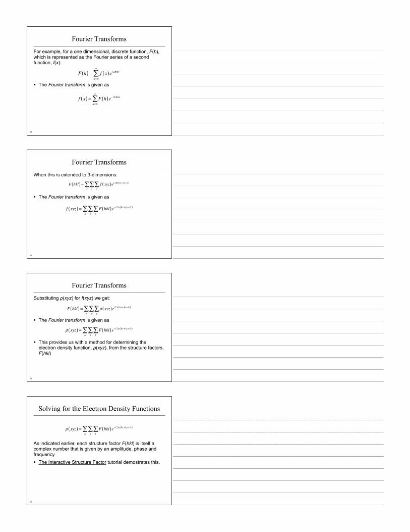
Fourier Transforms

For example, for a one dimensional, discrete function, F(h), which is represented as the Fourier series of a second function, f(x):

• The Fourier transform is given as

49

F h( ) = f x( )ei2 hx

x=0

f x( ) = F h( )e– i2 hx

h=0

Fourier Transforms

When this is extended to 3-dimensions:


50

F hkl( ) = f xyz( )ei2 hx+ ky+ lz( )

zyx

f xyz( ) = F hkl( )e– i2 hx+ ky+ lz( )

lkh

Fourier Transforms

Substituting (xyz) for f(xyz) we get:


• This provides us with a method for determining the electron density function, (xyz), from the structure factors, F(hkl)

51

F hkl( ) = xyz( )ei2 hx+ ky+ lz( )

zyx

xyz( ) = F hkl( )e– i2 hx+ ky+ lz( )

lkh

Solving for the Electron Density Functions

As indicated earlier, each structure factor F(hkl) is itself a complex number that is given by an amplitude, phase and frequency

• The Interactive Structure Factor tutorial demostrates this.

52

xyz( ) = F hkl( )e– i2 hx+ ky+ lz( )

lkh

Solving for the Electron Density Functions

• The frequency is determined by the Miller indices (h,k,l), which determine the frequency of the planes cutting through the unit cell.

• The amplitude of each structure factor |F(hkl)|, can be determined from the intensity of each spot I(hkl):

• What’s missing is the phase information- We have essentially taken a black-and-white photo instead of a colored one

53

F hkl( ) = I hkl( )

Solving the Phase Problem

For unit cells with small numbers of atoms, a Patterson Map can be used to determine the distances and directions between the atoms in the unit cell.

• A Patterson Map is constructed by assuming the phases are all zero

• The Interactive Structure Factor tutorial demostrates this.

54

P xyz( ) = F hkl( ) e– i2 hx+ ky+ lz( )

lkh


• Patterson Map

55


For protein crystals, can approximate this situation by using isomorphic replacement

• A small number of metal ions are introduced into the crystal.

Another method used to solve for the structure factor phoases is Molecular Replacement

• In this method a homologous protein with a known structure is packed into the cell and used used to determine the phases using an Inverse Fourier Transform

56

F hkl( )calc = xyz( )ei2 hx+ ky+ lz( )

zyx

Model Building

A model is fit to the electron density:

57

Model Building

The model can be used to calculate a new set of phases:

• And this is used to determine a calculated structure factor that can be compared to the observed structure factor:

58

R =F hkl( )obs F hkl( )calc

F hkl( )obs

F hkl( )calc = xyz( )model ei2 hx+ ky+ lz( )

zyx

Model Building

This is an iterative process

59

Documents

Chem 406 - Lecture 7 · Chem 406 - Lecture 7 ... Louis de Broglie ... calc = ()xyz ei2 ()hx +ky lz z y x Model Building A model is fit to the electron density: 57