Embed Size (px)
Citation preview
Chapter 6Queueing Models
Banks, Carson, Nelson & NicolDiscrete-Event System Simulation
PurposePurpose
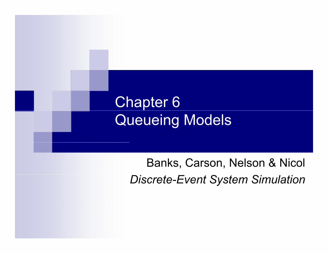
Simulation is often used in the analysis of queueing models.A simple but typical queueing model:
Queueing models provide the analyst with a powerful tool for d i i d l i h f f idesigning and evaluating the performance of queueing systems.Typical measures of system performance: yp y p
Server utilization, length of waiting lines, and delays of customersFor relatively simple systems, compute mathematicallyFor realistic models of complex systems simulation is usually
2
For realistic models of complex systems, simulation is usually required.
OutlineOutline
Discuss some well-known models (not development of queueing theories):
General characteristics of queues,Meanings and relationships of important performanceMeanings and relationships of important performance measures,Estimation of mean measures of performance.Effect of varying input parameters,Mathematical solution of some basic queueing models.
3
Characteristics of Queueing SystemsCharacteristics of Queueing Systems
Key elements of queueing systems:Customer: refers to anything that arrives at a facility and requires service, e.g., people, machines, trucks, emails.Server: refers to any resource that provides the requested service, e.g., repairpersons, retrieval machines, runways at airport.
4
Calling Population[Characteristics of Queueing System]
Calling population: the population of potential customers, b d t b fi it i fi itmay be assumed to be finite or infinite.
Finite population model: if arrival rate depends on the number of customers being served and waiting, e.g., model of one corporate jet, if it is being repaired, the repair arrival rate becomes zero.Infinite population model: if arrival rate is not affected by the number of customers being served and waiting, e.g., systems with large population of potential customers.
5
System Capacity[Characteristics of Queueing System]
System Capacity: a limit on the number of customers that may be in the waiting line or system.
Limited capacity, e.g., an automatic car wash only has room for 10 cars to wait in line to enter the mechanism.Unlimited capacity, e.g., concert ticket sales with no limit on the number of people allowed to wait to purchase tickets.
6
Arrival Process[Characteristics of Queueing System]
For infinite-population models:In terms of interarrival times of successive customers.Random arrivals: interarrival times usually characterized by a probability distribution.
Most important model: Poisson arrival process (with rate λ), where An represents the interarrival time between customer n-1 and customer n, and is exponentially distributed (with mean 1/λ).
S h d l d i l i t i l ti b t t t tScheduled arrivals: interarrival times can be constant or constant plus or minus a small random amount to represent early or late arrivals.
ti t t h i i h d l d i li fli ht i l te.g., patients to a physician or scheduled airline flight arrivals to an airport.
At least one customer is assumed to always be present, so the server is never idle e g sufficient raw material for a machine
7
server is never idle, e.g., sufficient raw material for a machine.

Arrival Process[Characteristics of Queueing System]
For finite-population models:Customer is pending when the customer is outside the queueing system, e.g., machine-repair problem: a machine is “pending” when it is operating, it becomes “not pending” the instant it d d i f th idemands service form the repairman.Runtime of a customer is the length of time from departure from the queueing system until that customer’s next arrival to the
hi i bl hi tqueue, e.g., machine-repair problem, machines are customers and a runtime is time to failure.Let A1
(i), A2(i), … be the successive runtimes of customer i, and
S (i) S (i) b th di i t tiS1(i), S2
(i) be the corresponding successive system times:
8
Queue Behavior and Queue Discipline[Characteristics of Queueing System]
Queue behavior: the actions of customers while in a queue waiting for service to begin for example:waiting for service to begin, for example:
Balk: leave when they see that the line is too long,Renege: leave after being in the line when its moving too slowly,J k f li h liJockey: move from one line to a shorter line.
Queue discipline: the logical ordering of customers in a queue that determines which customer is chosen for service when a server becomes free, for example:
First-in-first-out (FIFO)Last-in-first-out (LIFO)Service in random order (SIRO)Shortest processing time first (SPT)Service according to priority (PR).
9
Service Times and Service Mechanism[Characteristics of Queueing System]
Service times of successive arrivals are denoted by S1, S SS2, S3.
May be constant or random.{S1, S2, S3, …} is usually characterized as a sequence of { 1 2 3 } y qindependent and identically distributed random variables, e.g., exponential, Weibull, gamma, lognormal, and truncated normal distribution.
A queueing system consists of a number of service centers and interconnected queues.
Each service center consists of some number of servers cEach service center consists of some number of servers, c, working in parallel, upon getting to the head of the line, a customer takes the 1st available server.
10
Service Times and Service Mechanism[Characteristics of Queueing System]
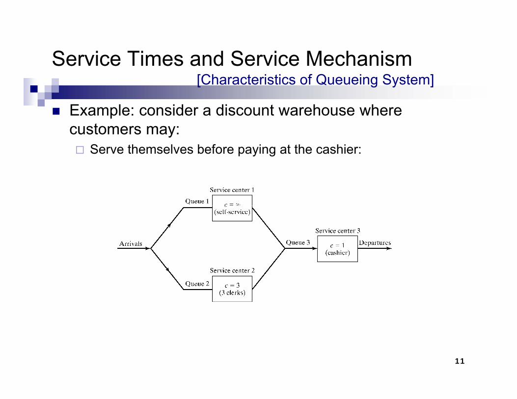
Example: consider a discount warehouse where tcustomers may:
Serve themselves before paying at the cashier:
11
Service Times and Service Mechanism[Characteristics of Queueing System]
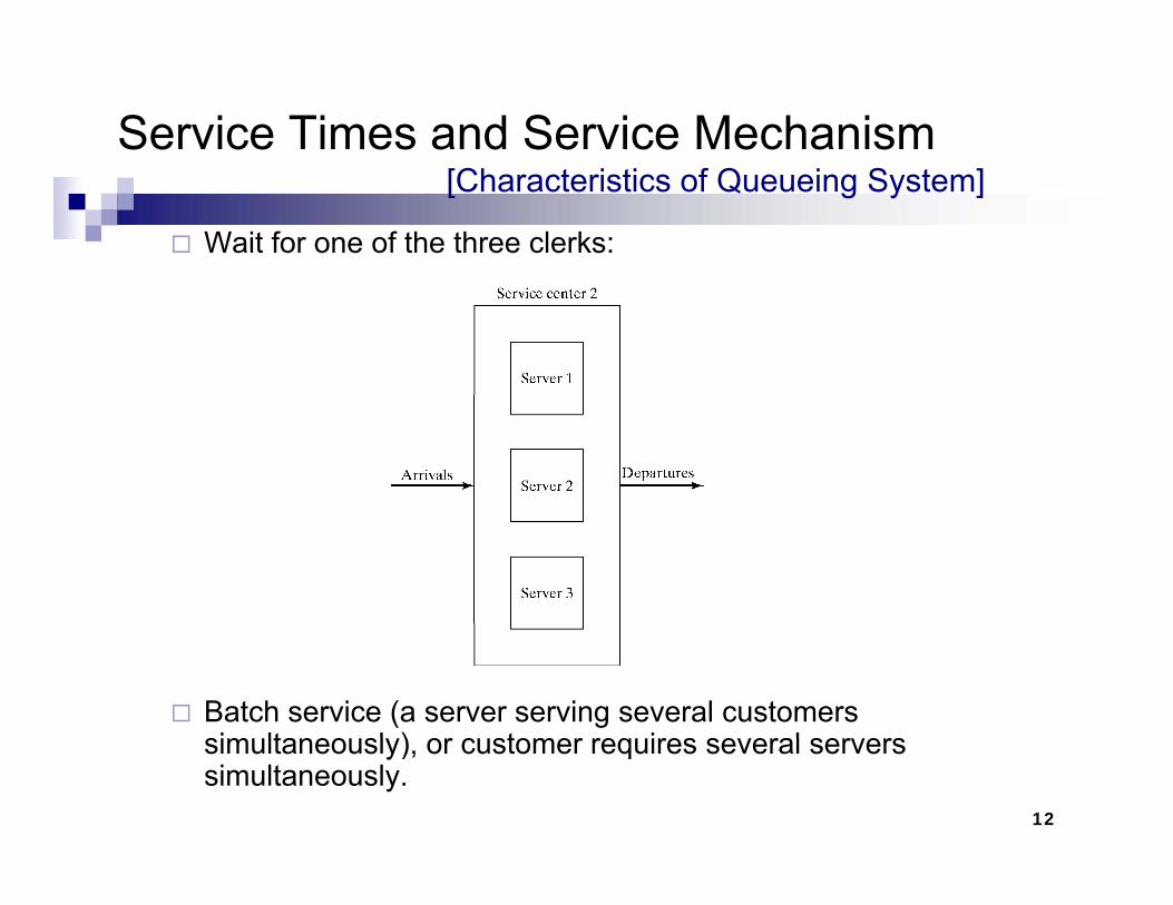
Wait for one of the three clerks:
Batch service (a server serving several customers sim ltaneo sl ) or c stomer req ires se eral ser ers
12
simultaneously), or customer requires several servers simultaneously.
Queueing Notation[Characteristics of Queueing System]
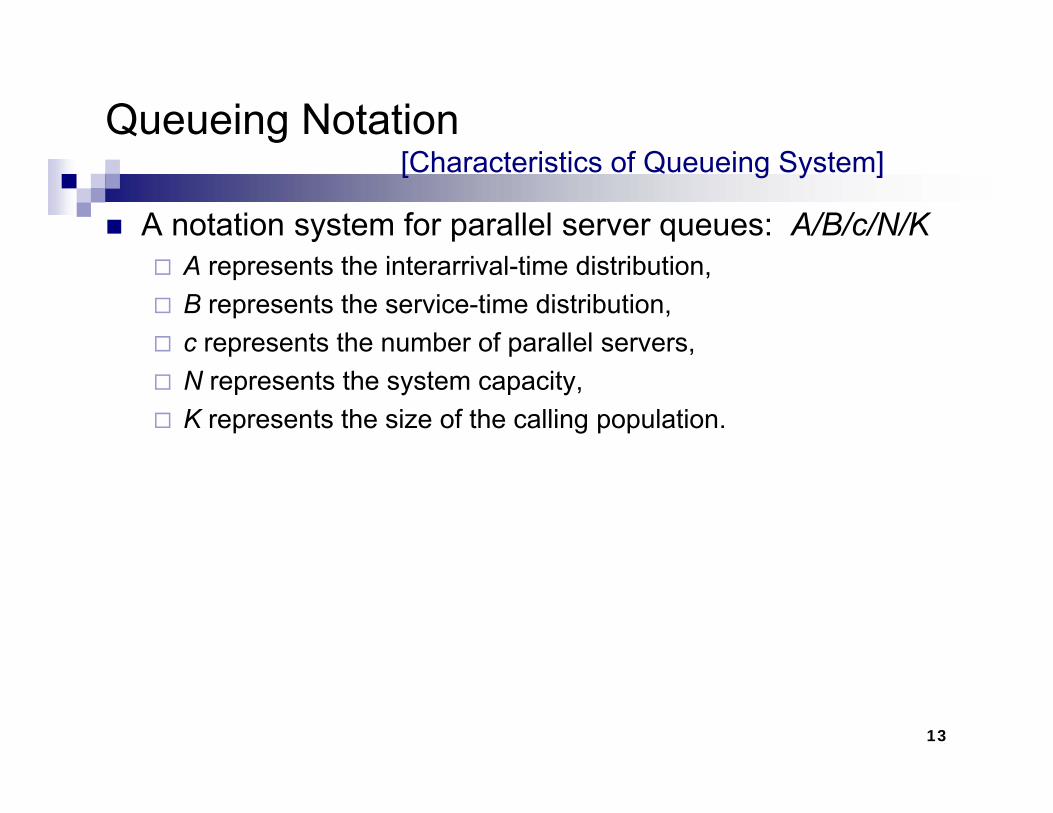
A notation system for parallel server queues: A/B/c/N/KA represents the interarrival-time distribution,B represents the service-time distribution,c represents the number of parallel servers,p pN represents the system capacity,K represents the size of the calling population.
13
Queueing Notation[Characteristics of Queueing System]
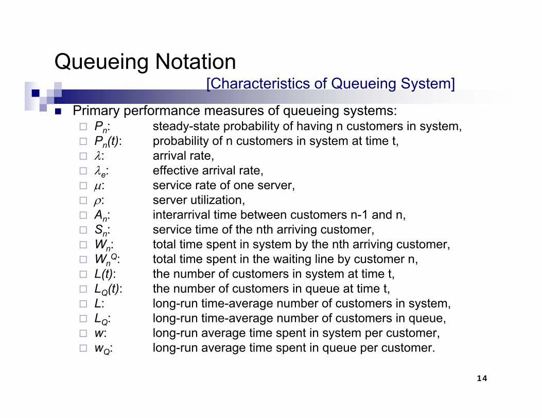
Primary performance measures of queueing systems:Pn: steady-state probability of having n customers in system,Pn: steady state probability of having n customers in system,Pn(t): probability of n customers in system at time t,λ: arrival rate,λe: effective arrival rate,
ser ice rate of one ser erµ: service rate of one server,ρ: server utilization,An: interarrival time between customers n-1 and n,Sn: service time of the nth arriving customer,n gWn: total time spent in system by the nth arriving customer,Wn
Q: total time spent in the waiting line by customer n,L(t): the number of customers in system at time t,L (t): the number of customers in queue at time tLQ(t): the number of customers in queue at time t,L: long-run time-average number of customers in system,LQ: long-run time-average number of customers in queue,w: long-run average time spent in system per customer,
14
wQ: long-run average time spent in queue per customer.
Time-Average Number in System L[Characteristics of Queueing System]
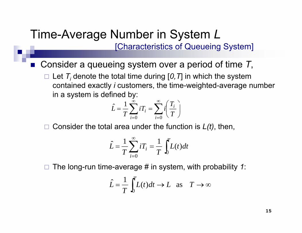
Consider a queueing system over a period of time T,Let Ti denote the total time during [0,T] in which the system contained exactly i customers, the time-weighted-average number in a system is defined by:
∞∞ ⎞⎛1 T
Consider the total area under the function is L(t), then,
∑∑∞
=
∞
=
⎟⎠
⎞⎜⎝
⎛==00
1ˆi
i
ii T
TiiT
TL
∫∑ ==∞
=
T
ii dttL
TiT
TL
00
)(11ˆ
The long-run time-average # in system, with probability 1:
∞→→= ∫ TLdttLT
LT
as )(1ˆ0
15
∫T 0
Time-Average Number in System L[Characteristics of Queueing System]
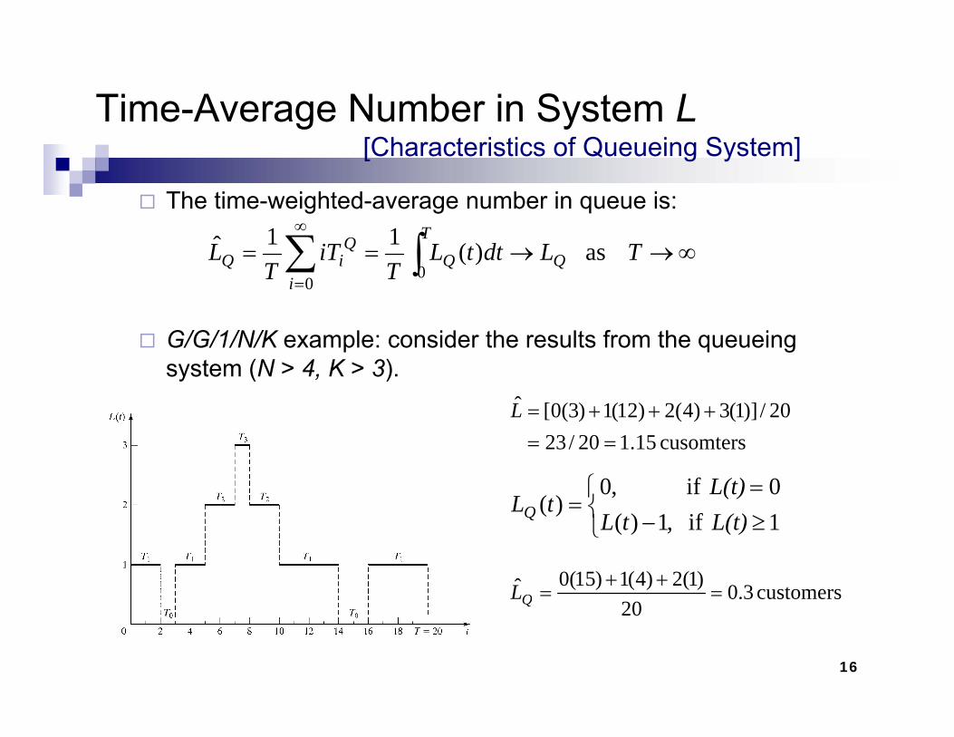
The time-weighted-average number in queue is:∞ T11
∞→→== ∫∑∞
=
TLdttLT
iTT
L QT
Qi
QiQ as )(11ˆ
00
G/G/1/N/K example: consider the results from the queueing system (N > 4, K > 3).
20/)]1(3)4(2)12(1)3(0[ˆ +++=L
⎨⎧ =
=0 if ,0
)(L(t)
tLQ
cusomters 15.120/2320/)]1(3)4(2)12(1)3(0[
==+++L
⎩⎨ ≥−
=1 if ,1)(
)(L(t)tL
tLQ
customers3.0)1(2)4(1)15(0ˆ =++
=QL
16
20Q
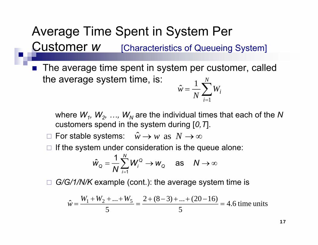
Average Time Spent in System Per Customer w [Ch t i ti f Q i S t ]Customer w [Characteristics of Queueing System]
The average time spent in system per customer, called th t ti ithe average system time, is:
∑=
=N
iiW
Nw
1
1ˆ
where W1, W2, …, WN are the individual times that each of the Ncustomers spend in the system during [0,T].For stable systems: ∞→→ Nww asˆFor stable systems:If the system under consideration is the queue alone:
∞→→ Nww as
1ˆ as N
QQ i Qw W w N
N= → → ∞∑
G/G/1/N/K example (cont.): the average system time is1iN =
)1620()38(2521 −++−++++ WWW
17
unitstime6.45
)1620(...)38(25
...ˆ 521 =+++
=+++
=WWW
w
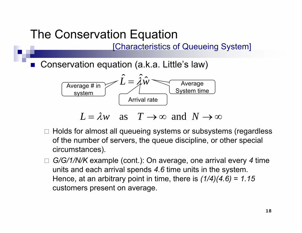
The Conservation Equation[Characteristics of Queueing System]
Conservation equation (a.k.a. Little’s law)
wL ˆˆˆ λ=
Arrival rate
Average System time
Average # in system
Holds for almost all queueing systems or subsystems (regardless
∞→∞→= NTwL and as λHolds for almost all queueing systems or subsystems (regardless of the number of servers, the queue discipline, or other special circumstances).G/G/1/N/K example (cont ): On average one arrival every 4 timeG/G/1/N/K example (cont.): On average, one arrival every 4 time units and each arrival spends 4.6 time units in the system. Hence, at an arbitrary point in time, there is (1/4)(4.6) = 1.15customers present on average.
18
customers present on average.
Server Utilization[Characteristics of Queueing System]
Definition: the proportion of time that a server is busy.Observed server utilization, , is defined over a specified time interval [0,T].Long-run server utilization is ρ.
ρ̂
For systems with long-run stability: ∞→→ T as ˆ ρρ
19
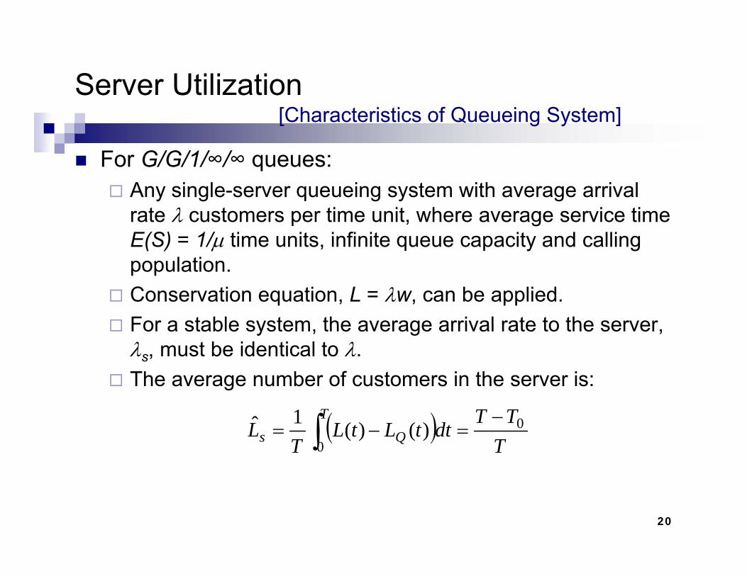
Server Utilization[Characteristics of Queueing System]
For G/G/1/∞/∞ queues:Any single-server queueing system with average arrival rate λ customers per time unit, where average service time E(S) = 1/µ time units, infinite queue capacity and calling population.Conservation equation, L = λw, can be applied.For a stable system the average arrival rate to the serverFor a stable system, the average arrival rate to the server, λs, must be identical to λ.The average number of customers in the server is:
( )T
TTdttLtL
TL
TQs
00
)()(1ˆ −=−= ∫
20
Server Utilization[Characteristics of Queueing System]
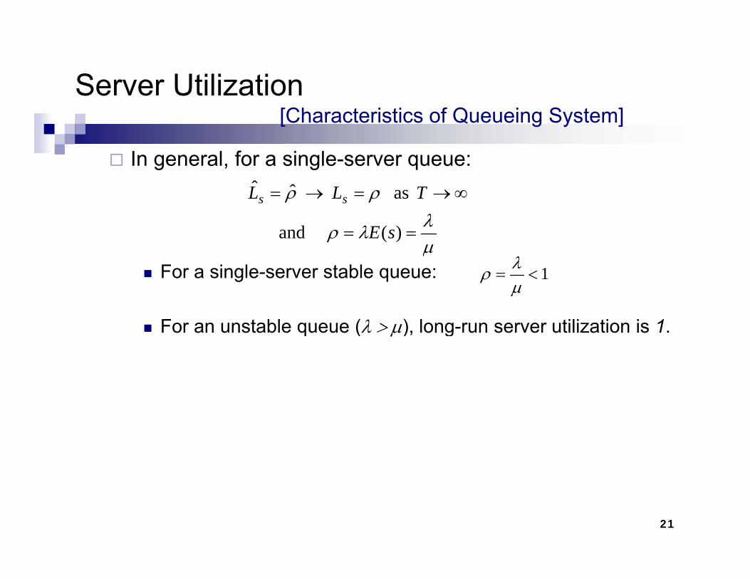
In general, for a single-server queue:
µλλρ
ρρ
==
∞→=→=
)( and
as ˆˆ
sE
TLL ss
For a single-server stable queue:
For an unstable queue (λ > µ) long run server utilization is 1
µ1<=
µλρ
For an unstable queue (λ > µ), long-run server utilization is 1.
21
Server Utilization[Characteristics of Queueing System]
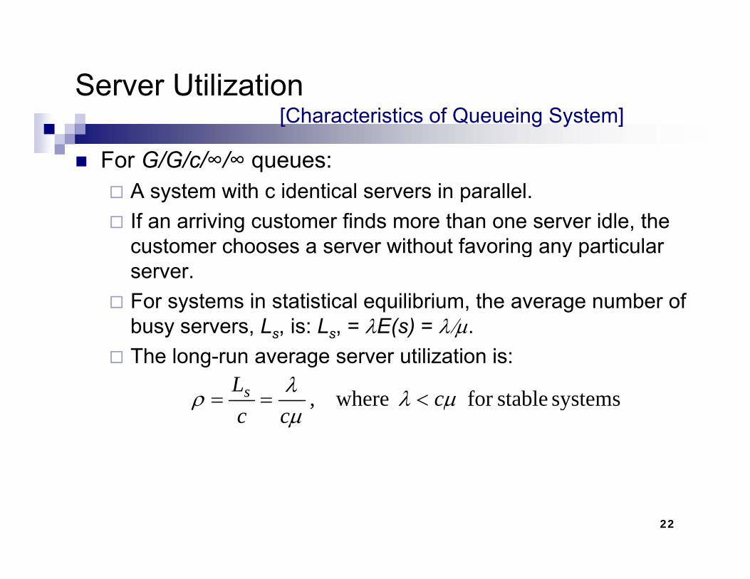
For G/G/c/∞/∞ queues:A system with c identical servers in parallel.If an arriving customer finds more than one server idle, the customer chooses a server without favoring any particular custo e c ooses a se e t out a o g a y pa t cu aserver.For systems in statistical equilibrium, the average number of busy servers L is: L = λE(s) = λ/µbusy servers, Ls, is: Ls, = λE(s) = λ/µ.The long-run average server utilization is:
systemsstableforwhere µλλρ cLs <== systemsstablefor where, µλ
µρ c
cc<==
22

Server Utilization and System Performance[Characteristics of Queueing System]
System performance varies widely for a given utilization ρ.For example, a D/D/1 queue where E(A) = 1/λ and E(S) = 1/µ, where:
L = ρ = λ/µ, w = E(S) = 1/µ, LQ = WQ = 0.ρ λ/µ, (S) /µ, Q Q 0By varying λ and µ, server utilization can assume any value between 0 and 1.Yet there is never any lineYet there is never any line.
In general, variability of interarrival and service times causes lines to fluctuate in length.
23
Server Utilization and System Performance[Characteristics of Queueing System]
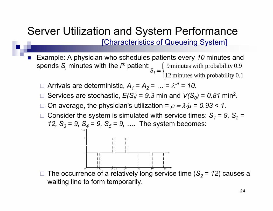
Example: A physician who schedules patients every 10 minutes and spends S minutes with the ith patient: ⎧ 90yprobabilitwithminutes9spends Si minutes with the ith patient:
Arrivals are deterministic, A1 = A2 = … = λ-1 = 10.⎩⎨⎧
=1.0y probabilit with minutes 12
9.0y probabilitwith minutes 9iS
Services are stochastic, E(Si) = 9.3 min and V(S0) = 0.81 min2.On average, the physician's utilization = ρ = λ/µ = 0.93 < 1.Consider the system is simulated with service times: S1 = 9, S2 = y 1 212, S3 = 9, S4 = 9, S5 = 9, …. The system becomes:
The occ rrence of a relati el long ser ice time (S 12) ca ses a
24
The occurrence of a relatively long service time (S2 = 12) causes a waiting line to form temporarily.
Costs in Queueing Problems[Characteristics of Queueing System]
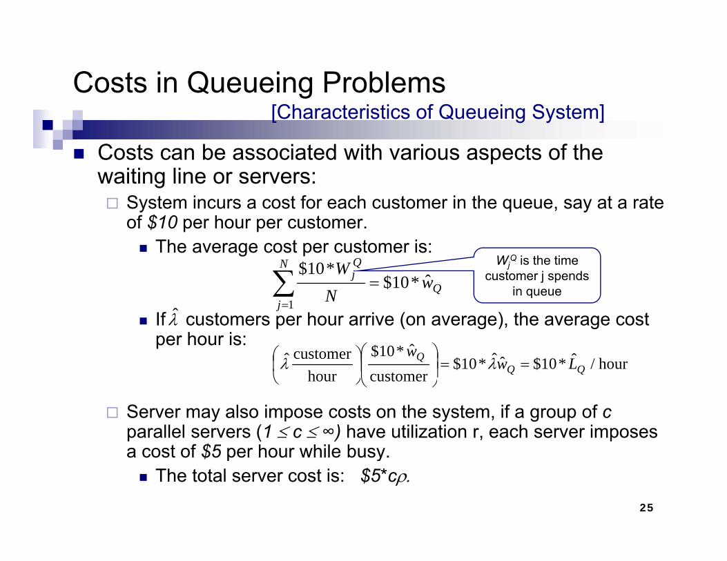
Costs can be associated with various aspects of the waiting line or servers:waiting line or servers:
System incurs a cost for each customer in the queue, say at a rate of $10 per hour per customer.
The average cost per customer is:The average cost per customer is:
If customers per hour arrive (on average) the average cost
Q
N
j
Qj w
NW
ˆ*10$*10$
1
=∑=
WjQ is the time
customer j spends in queue
λ̂If customers per hour arrive (on average), the average cost per hour is:
λ
hour / ˆ*10$ˆˆ*10$customer
ˆ*10$hour
customerˆQQ
Q Lww
==⎟⎟⎠
⎞⎜⎜⎝
⎛⎟⎠⎞
⎜⎝⎛ λλ
Server may also impose costs on the system, if a group of cparallel servers (1 ≤ c ≤ ∞) have utilization r, each server imposes a cost of $5 per hour while busy.
⎠⎝
25
a cost o $5 pe ou e busyThe total server cost is: $5*cρ.
Steady-State Behavior of Infinite-Population Markovian ModelsMarkovian Models
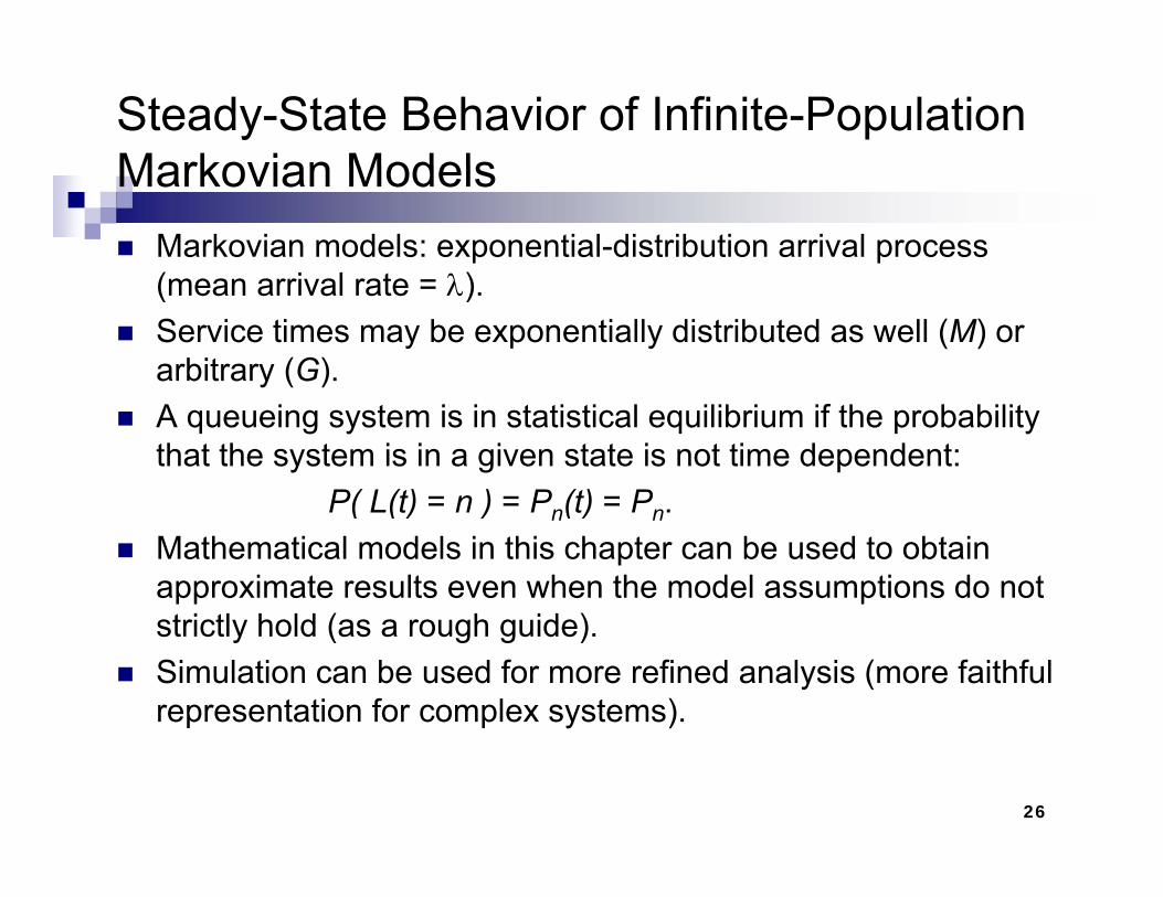
Markovian models: exponential-distribution arrival process (mean arrival rate λ)(mean arrival rate = λ).Service times may be exponentially distributed as well (M) or arbitrary (G).A queueing system is in statistical equilibrium if the probability that the system is in a given state is not time dependent:
P( L(t) = n ) = P (t) = PP( L(t) = n ) = Pn(t) = Pn.Mathematical models in this chapter can be used to obtain approximate results even when the model assumptions do not t i tl h ld ( h id )strictly hold (as a rough guide).
Simulation can be used for more refined analysis (more faithful representation for complex systems).
26
Steady-State Behavior of Infinite-Population Markovian ModelsMarkovian Models
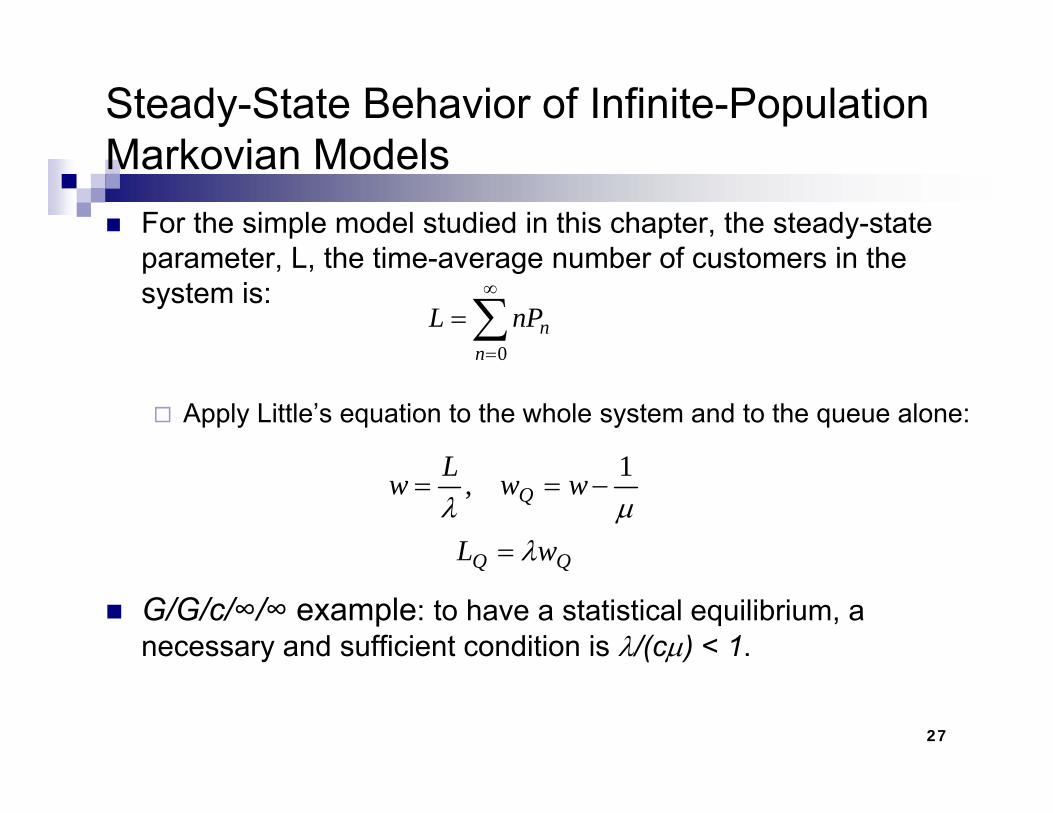
For the simple model studied in this chapter, the steady-state parameter L the time average number of customers in theparameter, L, the time-average number of customers in the system is:
∑∞
=
=0n
nnPL
Apply Little’s equation to the whole system and to the queue alone:
=0n
L 1
Q
wL
wwLw
λµλ
=
−==1 ,
G/G/c/∞/∞ example: to have a statistical equilibrium, a necessary and sufficient condition is λ/(cµ) < 1.
QQ wλ
27
M/G/1 Queues [Steady-State of Markovian Model]M/G/1 Queues [Steady State of Markovian Model]
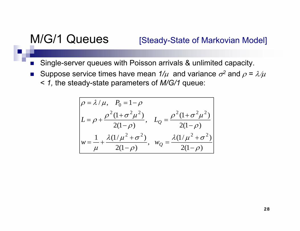
Single-server queues with Poisson arrivals & unlimited capacity.S i ti h 1/ d i 2 d λ/Suppose service times have mean 1/µ and variance σ2 and ρ = λ/µ< 1, the steady-state parameters of M/G/1 queue:
1/λ P
)1(2)1( ,
)1(2)1(
1 ,/222222
0
ρµσρ
ρµσρρ
ρµλρ
−+
=−
++=
−==
QLL
P
)1(2)/1( ,
)1(2)/1(1 2222
ρσµλ
ρσµλ
µ −+
=−
++= Qww
28

M/G/1 Queues [Steady-State of Markovian Model]M/G/1 Queues [Steady State of Markovian Model]
No simple expression for the steady-state probabilities P0, P1, … L L i th ti b f t b iL – LQ = ρ is the time-average number of customers being served.Average length of queue, LQ, can be rewritten as:
)1(2)1(2
222
ρσλ
ρρ
−+
−=QL
If λ and µ are held constant, LQ depends on the variability, σ2, of the service times.
29
M/G/1 Queues [Steady-State of Markovian Model]M/G/1 Queues [Steady State of Markovian Model]
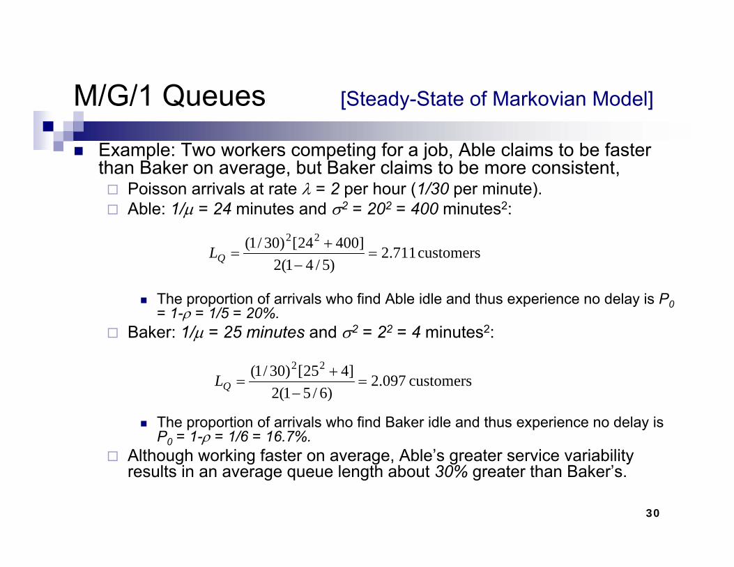
Example: Two workers competing for a job, Able claims to be faster than Baker on average, but Baker claims to be more consistent, g , ,
Poisson arrivals at rate λ = 2 per hour (1/30 per minute).Able: 1/µ = 24 minutes and σ2 = 202 = 400 minutes2:
7112]40024[)30/1( 22 +L
The proportion of arrivals who find Able idle and thus experience no delay is P0= 1-ρ = 1/5 = 20%.
customers711.2)5/41(2
]00[)30/(=
−=QL
ρBaker: 1/µ = 25 minutes and σ2 = 22 = 4 minutes2:
customers 097.2)6/51(2
]425[)30/1( 22=
+=QL
The proportion of arrivals who find Baker idle and thus experience no delay is P0 = 1-ρ = 1/6 = 16.7%.
Although working faster on average, Able’s greater service variability
)6/51(2 −Q
30
g g g , g yresults in an average queue length about 30% greater than Baker’s.
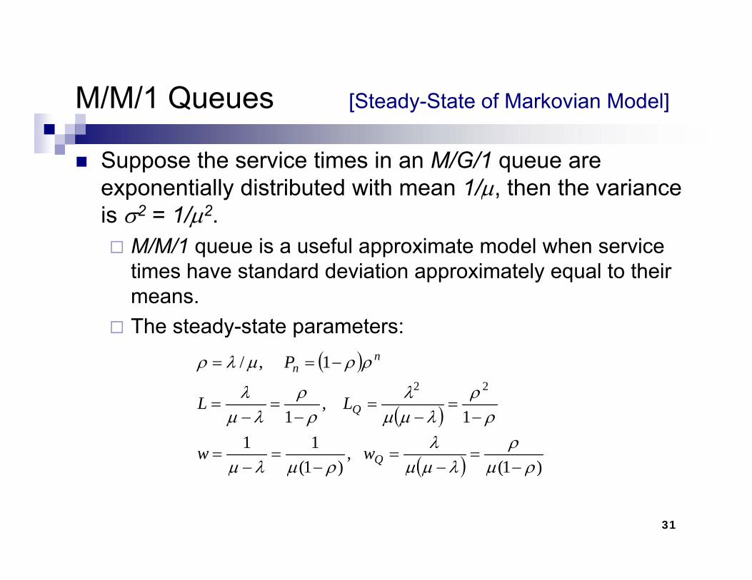
M/M/1 Queues [Steady-State of Markovian Model]M/M/1 Queues [Steady State of Markovian Model]
Suppose the service times in an M/G/1 queue are ti ll di t ib t d ith 1/ th th iexponentially distributed with mean 1/µ, then the variance
is σ2 = 1/µ2. M/M/1 queue is a useful approximate model when service q pptimes have standard deviation approximately equal to their means.The steady state parameters:The steady-state parameters:
( )1 ,/22 ρλρλ
ρρµλρ −== nn
LL
P
( )
( ) )1( ,
)1(11
1 ,
1
ρµρ
λµµλ
ρµλµ
ρρ
λµµρρ
λµ
−=
−=
−=
−=
−=
−=
−=
−=
Q
Q
ww
LL
31
( ) )()( ρµµµρµµ
M/M/1 Queues [Steady-State of Markovian Model]M/M/1 Queues [Steady State of Markovian Model]
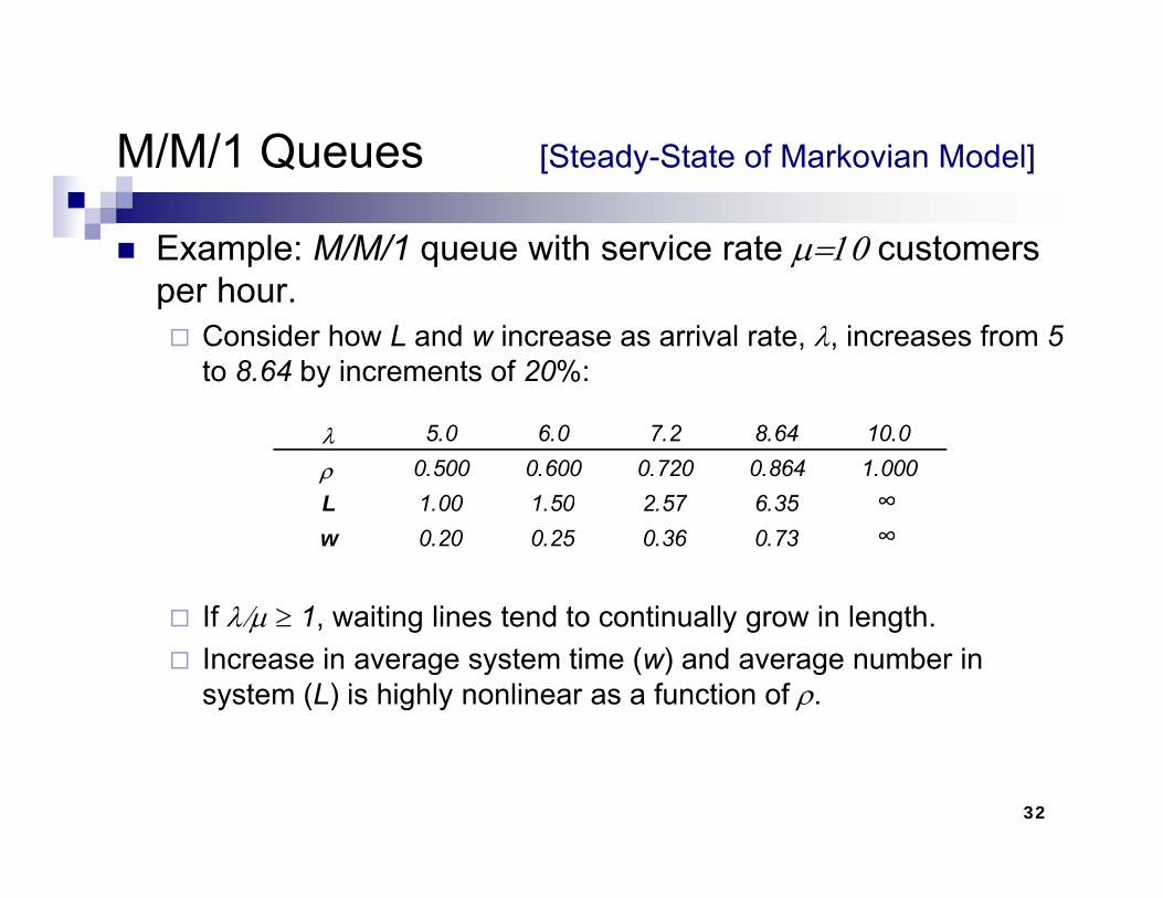
Example: M/M/1 queue with service rate µ=10 customers hper hour.
Consider how L and w increase as arrival rate, λ, increases from 5to 8.64 by increments of 20%:
λ 5.0 6.0 7.2 8.64 10.0ρ 0.500 0.600 0.720 0.864 1.000L 1 00 1 50 2 57 6 35 ∞
If λ/µ ≥ 1 waiting lines tend to continually grow in length
L 1.00 1.50 2.57 6.35w 0.20 0.25 0.36 0.73 ∞
If λ/µ ≥ 1, waiting lines tend to continually grow in length.Increase in average system time (w) and average number in system (L) is highly nonlinear as a function of ρ.
32
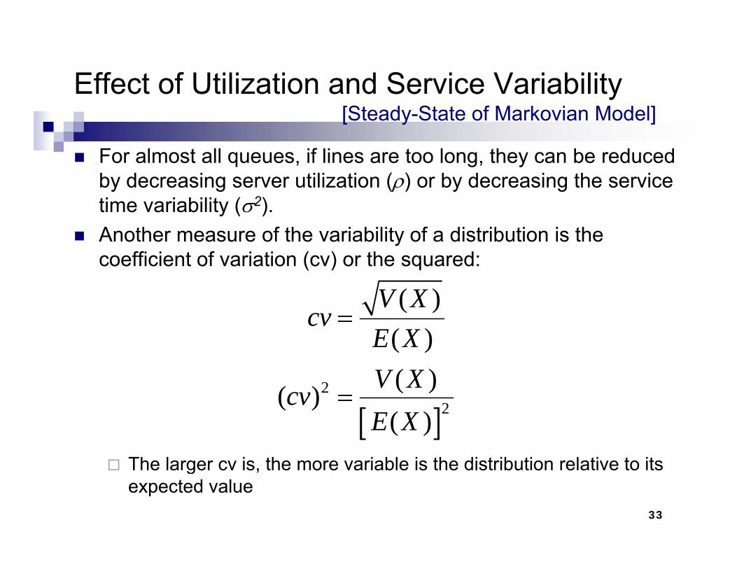
Effect of Utilization and Service Variability[Steady-State of Markovian Model]
For almost all queues, if lines are too long, they can be reduced by decreasing server utilization ( ) or by decreasing the serviceby decreasing server utilization (ρ) or by decreasing the service time variability (σ2).Another measure of the variability of a distribution is the coefficient of variation (cv) or the squared:
( )V Xcv =
2
( )( )( )
cvE XV X
=
The larger cv is the more variable is the distribution relative to its
[ ]2
2( )( )( )
cvE X
=
33
The larger cv is, the more variable is the distribution relative to its expected value
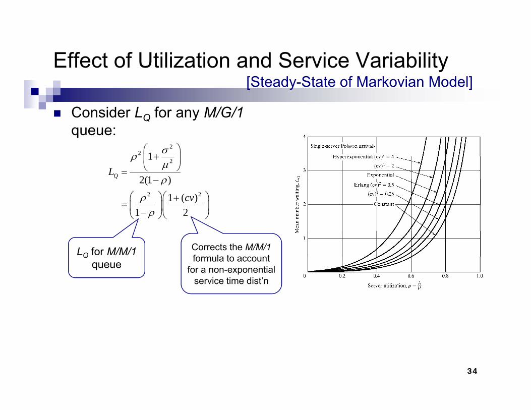
Effect of Utilization and Service Variability[Steady-State of Markovian Model]
Consider LQ for any M/G/1queue:queue:
22
21
2(1 )QL
σρµρ
⎛ ⎞+⎜ ⎟
⎝ ⎠=
2 2
2(1 )
1 ( )1 2
cv
ρ
ρρ
−
⎛ ⎞⎛ ⎞+= ⎜ ⎟⎜ ⎟−⎝ ⎠⎝ ⎠
LQ for M/M/1queue
Corrects the M/M/1formula to account
for a non-exponential service time dist’nservice time dist n
34
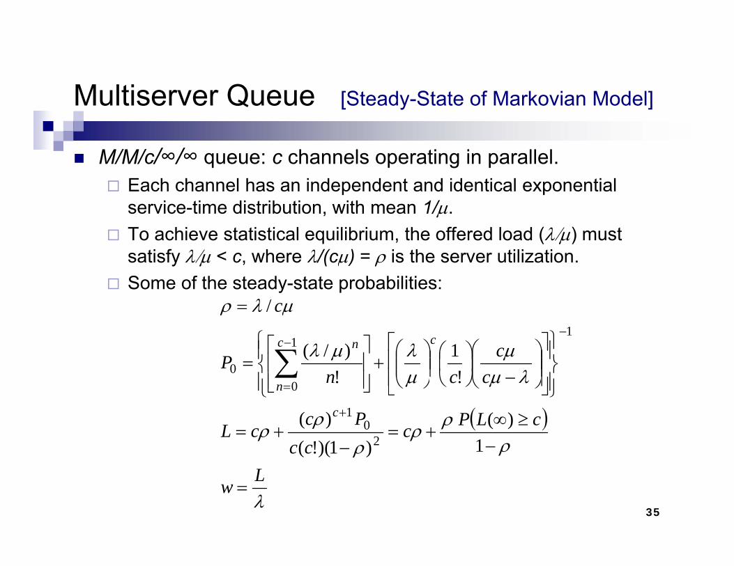
Multiserver Queue [Steady-State of Markovian Model]Multiserver Queue [Steady State of Markovian Model]
M/M/c/∞/∞ queue: c channels operating in parallel.Each channel has an independent and identical exponential service-time distribution, with mean 1/µ.To achieve statistical equilibrium, the offered load (λ/µ) must satisfy λ/µ < c, where λ/(cµ) = ρ is the server utilization.Some of the steady-state probabilities:
µλρ c= /
λµµ
µλµλ
cc
cnP
cc
n
n
⎪⎭
⎪⎬⎫
⎪⎩
⎪⎨⎧
⎥⎥⎦
⎤
⎢⎢⎣
⎡⎟⎟⎠
⎞⎜⎜⎝
⎛−
⎟⎠⎞
⎜⎝⎛
⎟⎟⎠
⎞⎜⎜⎝
⎛+
⎥⎥⎦
⎤
⎢⎢⎣
⎡=
−−
=∑ !
1!
)/(1
1
00
( )ρ
ρρρ
ρρ cLPc
ccPc
cLc
n
−≥∞
+=−
+=
⎪⎭⎪⎩ ⎦⎣⎦⎣+
1)(
)1)(!()(
20
1
0
35λLw =
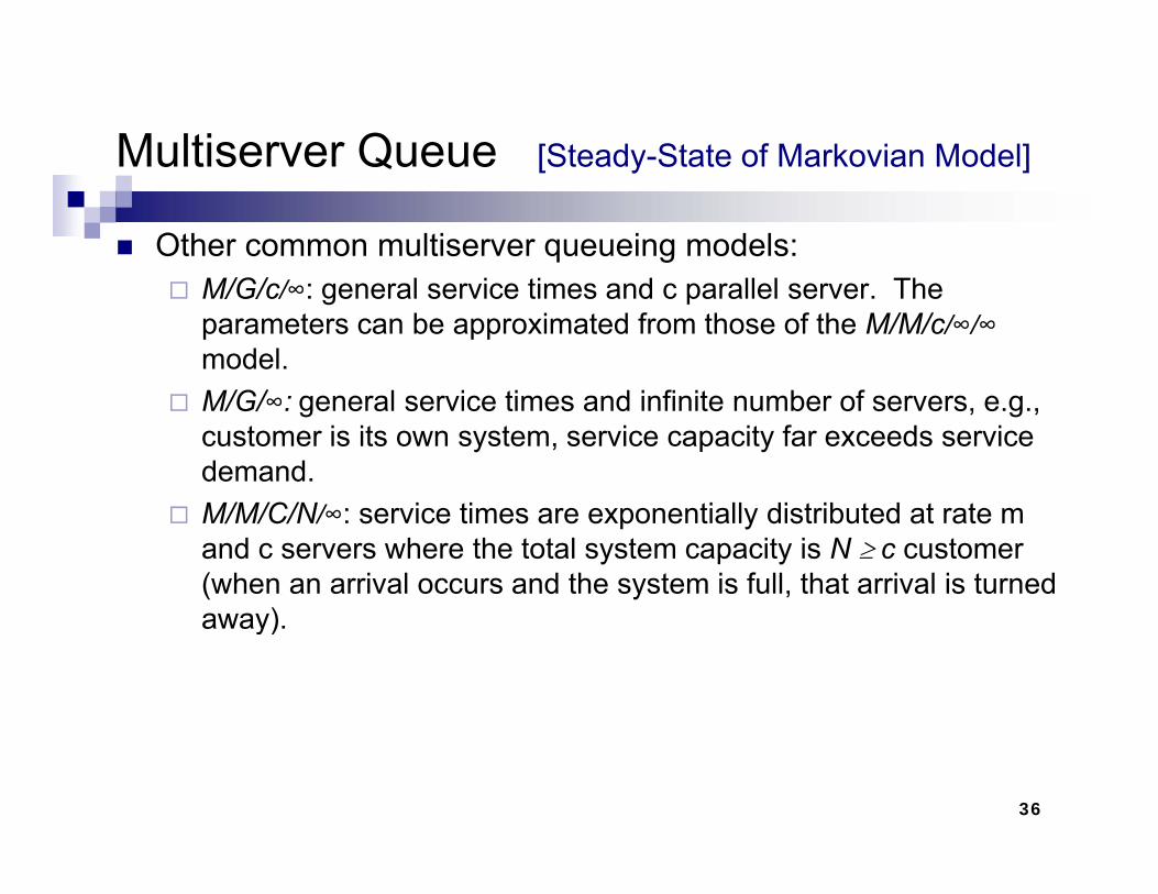
Multiserver Queue [Steady-State of Markovian Model]Multiserver Queue [Steady State of Markovian Model]
Other common multiserver queueing models:M/G/ l i i d ll l ThM/G/c/∞: general service times and c parallel server. The parameters can be approximated from those of the M/M/c/∞/∞model.M/G/ l i ti d i fi it b fM/G/∞: general service times and infinite number of servers, e.g., customer is its own system, service capacity far exceeds service demand.M/M/C/N i ti ti ll di t ib t d t tM/M/C/N/∞: service times are exponentially distributed at rate m and c servers where the total system capacity is N ≥ c customer (when an arrival occurs and the system is full, that arrival is turned away)away).
36
Steady-State Behavior of Finite-Population ModelsModels
When the calling population is small, the presence of one or more customers in the system has a strong effect on themore customers in the system has a strong effect on the distribution of future arrivals.Consider a finite-calling population model with K customers (M/M/c/K/K):
The time between the end of one service visit and the next call for service is exponentially distributed, (mean = 1/λ).Service times are also exponentially distributed.c parallel servers and system capacity is K.
37
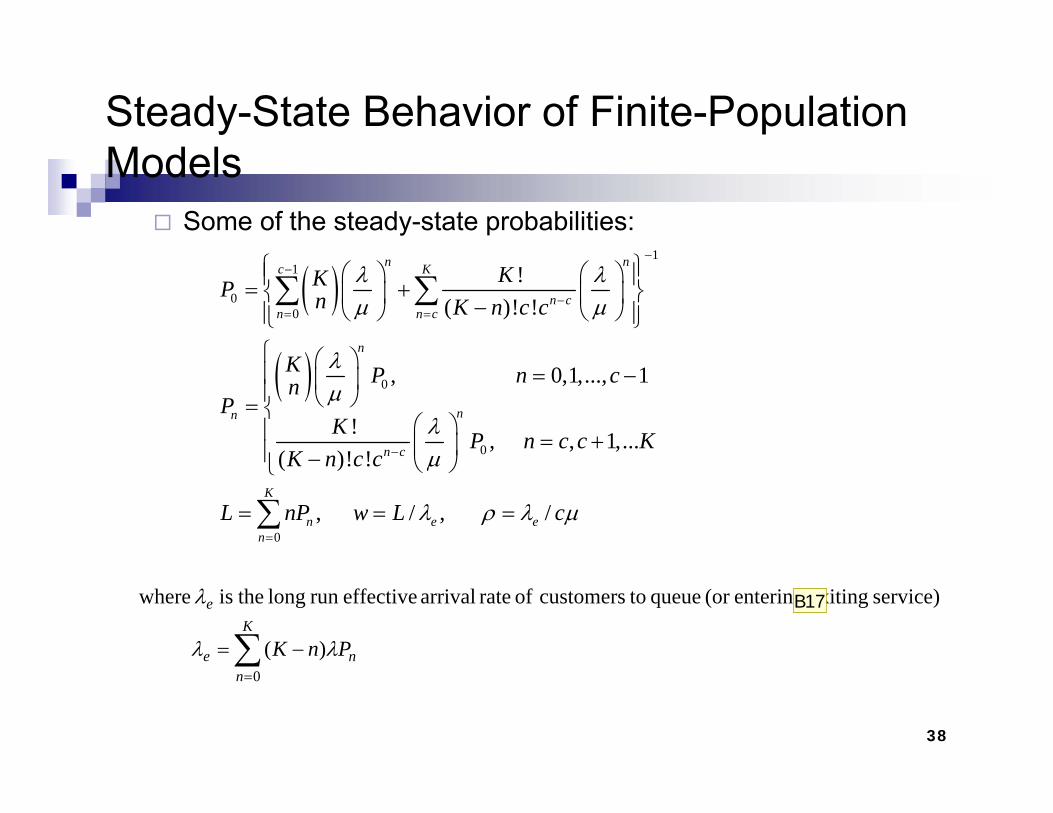
Steady-State Behavior of Finite-Population M d lModels
Some of the steady-state probabilities:1
( )
( )
11
00
!( )! !
n nc K
n cn n c
n
KKP n K n c cλ λµ µ
λ
−−
−= =
⎧ ⎫⎛ ⎞ ⎛ ⎞⎪ ⎪= +⎨ ⎬⎜ ⎟ ⎜ ⎟−⎝ ⎠ ⎝ ⎠⎪ ⎪⎩ ⎭⎧ ⎛ ⎞
∑ ∑
( ) 0
0
, 0,1,..., 1
! , , 1,...( )! !
nn
n c
K P n cnP
K P n c c KK n c c
λµ
λµ−
⎧ ⎛ ⎞⎪ = −⎜ ⎟⎪ ⎝ ⎠= ⎨
⎛ ⎞⎪ = +⎜ ⎟⎪ ⎝ ⎠⎩
0
( )! !
, / , /K
n e en
K n c c
L nP w L c
µ
λ ρ λ µ=
⎪ − ⎝ ⎠⎩
= = =∑
∑ −=K
ne
e
PnK )(
service) xitingentering/e(or queue tocustomers of rate arrival effectiverun long theis where
λλ
λ
38
∑=n 0
B17
Slide 38
B17 typo Brian; 2005/01/09

Steady-State Behavior of Finite-Population ModelsModels
Example: two workers who are responsible for10 milling machinesmachines.
Machines run on the average for 20 minutes, then require an average 5-minute service period, both times exponentially di t ib t d λ 1/20 d 1/5distributed: λ = 1/20 and µ = 1/5.All of the performance measures depend on P0:
065.05!1051011012
0 =⎪⎬⎫⎪
⎨⎧ ⎞
⎜⎛+⎞
⎜⎛⎞
⎜⎜⎛
=
−−
∑∑nn
P
Then, we can obtain the other Pn.Expected number of machines in system:
065.0202!2)!10(20 2
20
0⎪⎭⎬
⎪⎩⎨
⎠⎜⎝−
+⎠
⎜⎝⎠
⎜⎜⎝ =
−=
∑∑n
nn nn
P
The average number of running machines:
machines 17.310
0
== ∑=n
nnPL
39
g gmachines 83.617.310 =−=− LK
Networks of QueuesNetworks of Queues
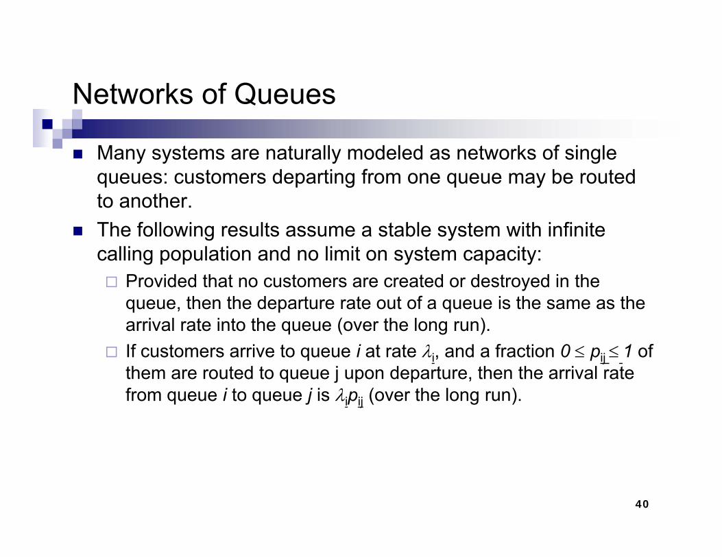
Many systems are naturally modeled as networks of single queues: customers departing from one queue may be routedqueues: customers departing from one queue may be routed to another.The following results assume a stable system with infinite calling population and no limit on system capacity:
Provided that no customers are created or destroyed in the queue, then the departure rate out of a queue is the same as the arrival rate into the queue (over the long run).If customers arrive to queue i at rate λi, and a fraction 0 ≤ pij ≤ 1 of them are routed to queue j upon departure, then the arrival rate from queue i to queue j is λipij (over the long run).
40
Networks of QueuesNetworks of Queues
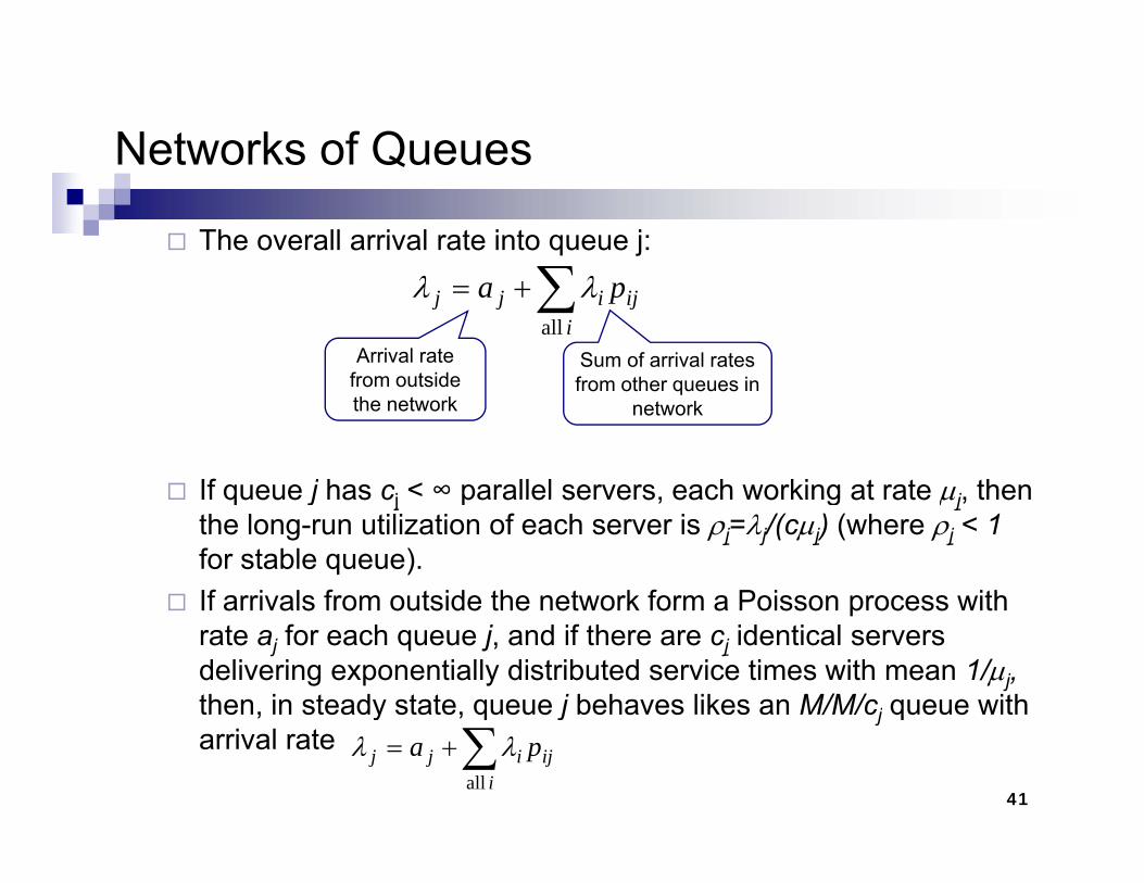
The overall arrival rate into queue j:
∑∑+=i
ijijj pa all
λλ
Arrival rate from outside
Sum of arrival rates from other queues in
If queue j has cj < ∞ parallel servers, each working at rate µj, then
from outside the network
from other queues in network
If queue j has cj parallel servers, each working at rate µj, then the long-run utilization of each server is ρj=λj/(cµj) (where ρj < 1for stable queue).If arrivals from outside the network form a Poisson process withIf arrivals from outside the network form a Poisson process with rate aj for each queue j, and if there are cj identical servers delivering exponentially distributed service times with mean 1/µj,then, in steady state, queue j behaves likes an M/M/cj queue with
41
y q j j qarrival rate ∑+=
iijijj pa
all
λλ
Network of QueuesNetwork of Queues
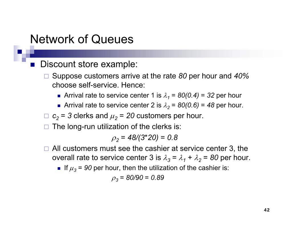
Discount store example: Suppose customers arrive at the rate 80 per hour and 40%choose self-service. Hence:
Arrival rate to service center 1 is λ1 = 80(0.4) = 32 per hourArrival rate to service center 2 is λ2 = 80(0.6) = 48 per hour.
c2 = 3 clerks and µ2 = 20 customers per hour.The long-run utilization of the clerks is:
ρ2 = 48/(3*20) = 0.8All customers must see the cashier at service center 3, the overall rate to service center 3 is λ3 = λ1 + λ2 = 80 per hour.overall rate to service center 3 is λ3 λ1 λ2 80 per hour.
If µ3 = 90 per hour, then the utilization of the cashier is:ρ3 = 80/90 = 0.89
42
SummarySummary Introduced basic concepts of queueing models.Sh h i l ti d ti th ti l l iShow how simulation, and some times mathematical analysis, can be used to estimate the performance measures of a system.Commonly used performance measures: L, LQ, w, wQ, ρ, and λe.When simulating any system that evolves over time, analyst must decide whether to study transient behavior or steady-state behavior.
Simple formulas exist for the steady-state behavior of some queues.Simple models can be solved mathematically, and can be useful in providing a rough estimate of a performance measure.
43