Introduction to Queueing Networkscslui/CSC5420/queueing_network_beamer.pdf · Introduction to Queueing Networks ... Theory on Jackson Networks Examples 3 Closed Queueing Network Example

Introduction to Queueing Networks

Prof. John C.S. LuiDepartment of Computer Science & Engineering

The Chinese University of Hong Kong

John C.S. Lui () Computer System Performance Evaluation 1 / 79

Outline

Outline

1 IntroductionIllustration

2 Jackson NetworkExampleTheory on Jackson NetworksExamples

3 Closed Queueing NetworkExampleTheory of Closed Queueing NetworkComputation MethodsConvolution AlgorithmMulticlass Queueing NetworksBCMP NetworksMean Value Analysis (MVA)


Introduction Illustration

Example: Network of Queues

µ 0 µ 1!

0,0 1,0 2,0

0,1 1,1

0,2

,0k0

k0 -1,1

! ! ! !

! ! !

!

µ 1 µ 0µ 1 µ 0

µ 1µ 1

µ 0

µ 1 µ 0µ 1

µ 1

!

!

.........

.........

.........

.........

.........



for k0 > 0, k1 > 0:

(µ0 +µ1 +λ)p(k0, k1) = µ0p(k0 +1, k1−1)+µ1p(k0, k1 +1)+λp(k0−1, k1)

for k0 > 0, k1 = 0:

(µ0 + λ)p(k0,0) = µ1p(k0,1) + λp(k0 − 1,0)

for k0 = 0, k1 > 0:

(µ1 + λ)p(0, k1) = µ0p(1, k1 − 1) + µ1p(0, k1 + 1)

for k0 = 0, k1 = 0:λp(0,0) = µ1p(0,1)



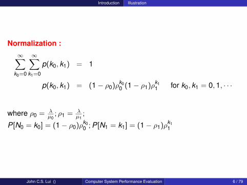
Normalization :∞∑

k0=0

∞∑k1=0

p(k0, k1) = 1

p(k0, k1) = (1− ρ0)ρk00 (1− ρ1)ρk1

1 for k0, k1 = 0,1, · · ·

where ρ0 = λµ0

; ρ1 = λµ1

;

P[N0 = k0] = (1− ρ0)ρk00 ; P[N1 = k1] = (1− ρ1)ρk1

1


Jackson Network Example

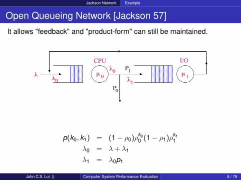
Open Queueing Network [Jackson 57]

It allows "feedback" and "product-form" can still be maintained.

µ 0 µ 1!

P0

P1!0

!0!1

CPU I/O

p(k0, k1) = (1− ρ0)ρk00 (1− ρ1)ρk1

1

λ0 = λ+ λ1

λ1 = λ0p1



Therefore,

λ0 =λ

1− p1

λ1 =λp1

1− p1

ρ0 =λ0

µ0=

λ

(1− p1)µ0=

λ

p0µ0

ρ1 =λ1

µ1=

λp1

p0µ1

What is the average response time of a job?



By Little’s formula, T = N̄λ where N̄ is the average no. of jobs in the

"system".

N̄ = N̄0 + N̄1 =∞∑

k0=0

∞∑k1=0

(k0 + k1)p(k0, k1)

=∞∑

k0=0

∞∑k1=0

k0p(k0, k1) +∞∑

k0=0

∞∑k1=0

k1p(k0, k1)

=∞∑

k0=0

k0(1− ρ0)ρk00

∞∑k1=0

(1− ρ1)ρk11

+∞∑

k0=0

(1− ρ0)ρk00

∞∑k1=0

k1(1− ρ1)ρk11

N̄ =ρ0

1− ρ0+

ρ1

1− ρ1; E [T ] =

N̄λ

=

[ρ0

1− ρ0+

ρ1

1− ρ1

] [1λ

]John C.S. Lui () Computer System Performance Evaluation 10 / 79


Types of service centersFCFS and service time is exponentially distributed.Processor sharing (PS)Last come first serve pre-emptive resume (LCFS-PR)Infinite server (IS) or delay nodes

We also allow a state dependent service rate (µi(n) = service rateat the i th node where there is n customer).

Single server fixed rate (SSFR) where µi (n) = uiInfinite server (IS) , µi (n) = nµiQueue length dependent (QLD) with service rate µi (n)


Jackson Network Theory on Jackson Networks

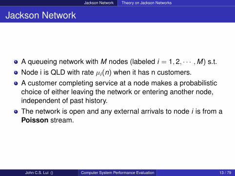
Jackson Network

A queueing network with M nodes (labeled i = 1,2, · · · ,M) s.t.Node i is QLD with rate µi(n) when it has n customers.A customer completing service at a node makes a probabilisticchoice of either leaving the network or entering another node,independent of past history.The network is open and any external arrivals to node i is from aPoisson stream.



Jackson Network : Continue

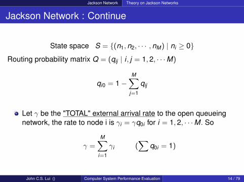
State space S = {(n1,n2, · · · ,nM) | ni ≥ 0}

Routing probability matrix Q = (qij | i , j = 1,2, · · ·M)

qi0 = 1−M∑

j=1

qij

Let γ be the "TOTAL" external arrival rate to the open queueingnetwork, the rate to node i is γi = γq0i for i = 1,2, · · ·M. So

γ =M∑

i=1

γi (∑

q0i = 1)



All nodes in the Jackson network are QLD with exponentialservice time. Pictorially we can have:

!1"1

"2

"3

!2

!3

!4

M=4

Let λi = mean arrival rate to node i,(i = 1,2, · · · ,M)

λi = γi +M∑

j=1

λjqji there is unique solution to{λi}



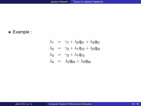
Example :

λ1 = γ1 + λ2q21 + λ3q31

λ2 = γ2 + λ1q12 + λ2q22

λ3 = γ3 + λ1q13

λ4 = λ2q24 + λ3q34



Jackson’s Theorem: For a Jackson Network in steady state witharrival rate λi to node i ,

The no. of customer at any node is independent of the number ofcustomers at every other node.Node i behaves "stochastically" as if it were subjected to Poissonarrival rates λi

Let π(~n) = Prob[(n1,n2, · · · nM)] where ni ≥ 0, for SSFR:

π(~n) =M∏

i=1

(1− λi

µi

)(λi

µi

)ni

For QLD, M/M/c queues, define ui(r) = µi min(r , ci) for r ≥ 0,i = 1, ..,M, and ρi = λi/µi for i = 1, ..M.

π(~n)=M∏

i=1

Ci

(λni

i∏nir=1 µi(r)

); Ci =

ci−1∑r=0

ρri

r !+

(ρci

ici !

)(1

1− ρi/ci

)−1



The i th node:

0 1 2

!i !i !i !i

µi(1) µi(2)µi(3) µi( )ni -1 (ni)µi

............

!i

ni -1 ni

How about the normalization constant Ci ?

π(~n) = π(n1,n2, · · · ,nM) =M∏

i=1

πi(ni) =M∏

i=1

Ci

[λni

i∏nij=1 µi(j)

]

where Ci can be found by∑∞

ni =0 Ci

[λ

niiQni

j=1 µi (j)

]= 1



So , what do we have?extremely powerful modeling tool to model a very large class ofsystem.efficient solutionwe can compute mean queue length, utilization and throughoutmean response time.



Comment

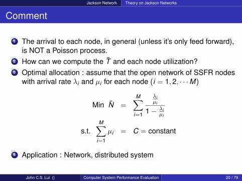
1 The arrival to each node, in general (unless it’s only feed forward),is NOT a Poisson process.

2 How can we compute the T̄ and each node utilization?3 Optimal allocation : assume that the open network of SSFR nodes

with arrival rate λi and µi for each node (i = 1,2, · · ·M)

Min N̄ =M∑

i=1

λiµi

1− λiµi

s.t.M∑

i=1

µi = C = constant

4 Application : Network, distributed system


Jackson Network Examples

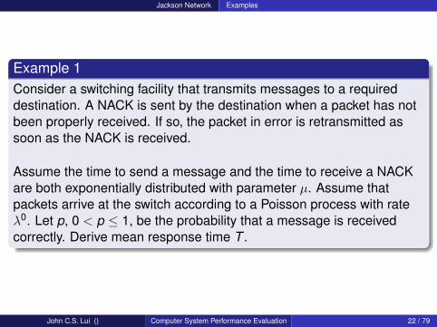
Example 1Consider a switching facility that transmits messages to a requireddestination. A NACK is sent by the destination when a packet has notbeen properly received. If so, the packet in error is retransmitted assoon as the NACK is received.

Assume the time to send a message and the time to receive a NACKare both exponentially distributed with parameter µ. Assume thatpackets arrive at the switch according to a Poisson process with rateλ0. Let p, 0 < p ≤ 1, be the probability that a message is receivedcorrectly. Derive mean response time T .



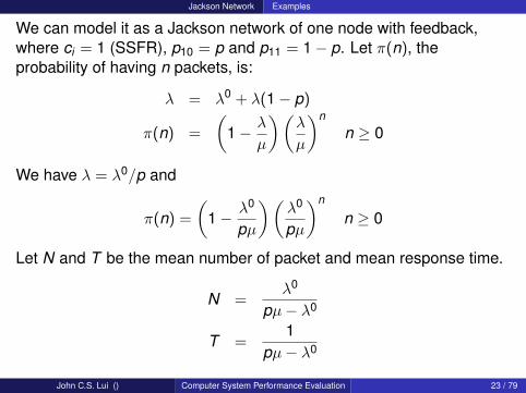
We can model it as a Jackson network of one node with feedback,where ci = 1 (SSFR), p10 = p and p11 = 1− p. Let π(n), theprobability of having n packets, is:

λ = λ0 + λ(1− p)

π(n) =

(1− λ

µ

)(λ

µ

)n

n ≥ 0

We have λ = λ0/p and

π(n) =

(1− λ0

pµ

)(λ0

pµ

)n

n ≥ 0

Let N and T be the mean number of packet and mean response time.

N =λ0

pµ− λ0

T =1

pµ− λ0



Example 2Similar to last example but now the switching facility is composed of Knodes in series, each model as M/M/1 queue with switching rate µ.What is the response time T ?

We have λ0i = 0 for i = 2, ...,K (no external arrival to nodes

2, ...,K ), µi = µ for i = 1,2, ...,K , pi,i+1 = 1 for i = 1, ...,K − 1, andpK ,0 = p and pK ,1 = 1− p.λ1 = λ0 + (1− p)λK , λi = λi−1 for i = 2, ...,K . So

λi = λ0/p ∀i = 1, ...,K .



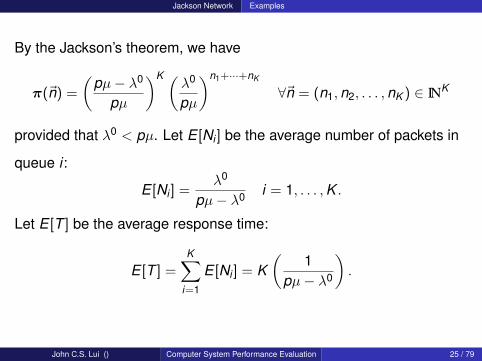
By the Jackson’s theorem, we have

π(~n) =

(pµ− λ0

pµ

)K (λ0

pµ

)n1+···+nK

∀~n = (n1,n2, . . . ,nK ) ∈ INK

provided that λ0 < pµ. Let E [Ni ] be the average number of packets in

queue i :

E [Ni ] =λ0

pµ− λ0 i = 1, . . . ,K .

Let E [T ] be the average response time:

E [T ] =K∑

i=1

E [Ni ] = K(

1pµ− λ0

).



Example 3: open central server networkA computer system with one CPU and two I/O devices. New jobsenter the system, wait for CPU resource, then possibly an I/Orequests. When a job finishes its I/O, it may return for more CPUresource. Eventually a job completes and leave the system.It means that K = 3 (three nodes). λ0

i = 0 for i = 2,3,p2,1 = p3,1 = 1, while p1,0 > 0.The traffic equations are: λ1 = λ0

1 + λ2 + λ3, λ2 = λ1p1,2,λ3 = λ1p1,3. Solving, we have: λ1 = λ0

1/p1,0, λi = λ01p1,i/p1,0 for

i = 2,3. Thus,

π(~n)=

(1−

λ01

µ1p1,0

)(λ0

1µ1p1,0

)n1 3∏i=2

(1−

λ01p1,i

µip1,0

)(λ0

1p1,i

µip1,0

)ni

~n ∈ IN3

E [T ] =1

µ1p1,0 − λ01

+3∑

i=2

p1,i

µip1,0 − λ01p1,i


Closed Queueing Network Example

Example of Queueing Network

We fixed the total number of jobs be n in the system, where n isalso called the “degree of multiprogramming”.

µ 0 µ 1

P0

P1!0!1

CPU I/O

new program path

State representation (k0, k1). Now with the constant thatk0 + k1 = n



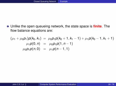
Unlike the open queueing network, the state space is finite. Theflow balance equations are:

(µ1 + µ0p1)p(k0, k1) = µ0p1p(k0 + 1, k1 − 1) + µ1p(k0 − 1, k1 + 1)

µ1p(0,n) = µ0p1p(1,n − 1)

µ0p1p(n,0) = µ1p(n − 1,1)



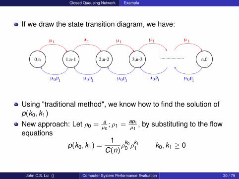
If we draw the state transition diagram, we have:

0,n 1,n-1 2,n-2 3,n-3 n,0

µ1 µ1 µ1 µ1 µ1

µ0p1 µ0p1 µ0p1 µ0p1 µ0p1

...................

Using "traditional method", we know how to find the solution ofp(k0, k1)

New approach: Let ρ0 = aµ0

; ρ1 = ap1µ1

, by substituting to the flowequations

p(k0, k1) =1

C(n)ρk0

0 ρk11 k0, k1 ≥ 0



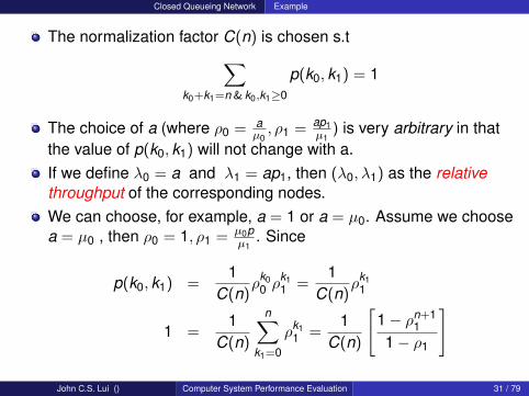
The normalization factor C(n) is chosen s.t∑k0+k1=n & k0,k1≥0

p(k0, k1) = 1

The choice of a (where ρ0 = aµ0, ρ1 = ap1

µ1) is very arbitrary in that

the value of p(k0, k1) will not change with a.If we define λ0 = a and λ1 = ap1, then (λ0, λ1) as the relativethroughput of the corresponding nodes.We can choose, for example, a = 1 or a = µ0. Assume we choosea = µ0 , then ρ0 = 1, ρ1 = µ0p

µ1. Since

p(k0, k1) =1

C(n)ρk0

0 ρk11 =

1C(n)

ρk11

1 =1

C(n)

n∑k1=0

ρk11 =

1C(n)

[1− ρn+1

11− ρ1

]



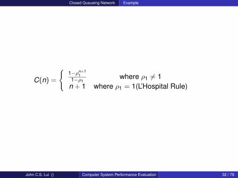
C(n) =

{1−ρn+1

11−ρ1

where ρ1 6= 1n + 1 where ρ1 = 1(L’Hospital Rule)



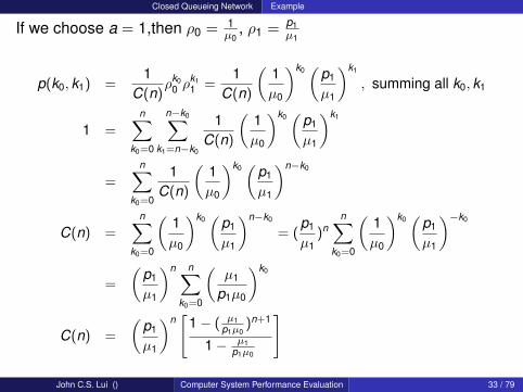
If we choose a = 1,then ρ0 = 1µ0

, ρ1 = p1µ1

p(k0, k1) =1

C(n)ρk0

0 ρk11 =

1C(n)

(1µ0

)k0(

p1

µ1

)k1

, summing all k0, k1

1 =n∑

k0=0

n−k0∑k1=n−k0

1C(n)

(1µ0

)k0(

p1

µ1

)k1

=n∑

k0=0

1C(n)

(1µ0

)k0(

p1

µ1

)n−k0

C(n) =n∑

k0=0

(1µ0

)k0(

p1

µ1

)n−k0

= (p1

µ1)n

n∑k0=0

(1µ0

)k0(

p1

µ1

)−k0

=

(p1

µ1

)n n∑k0=0

(µ1

p1µ0

)k0

C(n) =

(p1

µ1

)n[

1− ( µ1p1µ0

)n+1

1− µ1p1µ0

]



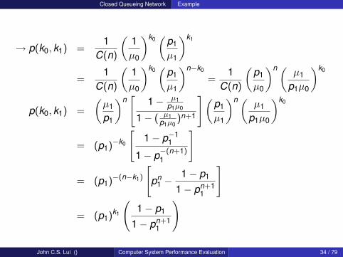
→ p(k0, k1) =1

C(n)

(1µ0

)k0(

p1

µ1

)k1

=1

C(n)

(1µ0

)k0(

p1

µ1

)n−k0

=1

C(n)

(p1

µ0

)n ( µ1

p1µ0

)k0

p(k0, k1) =

(µ1

p1

)n[

1− µ1p1µ0

1− ( µ1p1µ0

)n+1

](p1

µ1

)n ( µ1

p1µ0

)k0

= (p1)−k0

[1− p−1

1

1− p−(n+1)1

]

= (p1)−(n−k1)

[pn

1 −1− p1

1− pn+11

]

= (p1)k1

(1− p1

1− pn+11

)



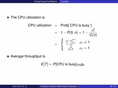
The CPU utilization is

CPU utilization = Prob[ CPU is busy ]

= 1− P(0,n) = 1−ρn

1C(n)

=

ρ1−ρn+1

11−ρn+1

1ρ1 6= 1

nn+1 ρ1 = 1

Average throughput is

E [T ] = P[CPU is busy]µ0p0


Closed Queueing Network Theory of Closed Queueing Network

Gordon - Newell network (1967)

A Gordon-Newell network has M nodes (i = 1,2, · · ·M) s.t.Node i is QLD with rate µi (n) when there is n customers.a customer completing service at a node chooses a node to enternext probabilistically, independent of past historyThe network is CLOSED and has a fixed population K

State space:S = {(n1,n2, · · · nM) | ni ≥ φ,∑M

i=1 ni = K}

|S| =

(K + M − 1

M − 1

)→ VERY LARGE NUMBER

If M = 5, K = 10, |S| = 1,001.If M = 10, K = 35, |S| = 52,451,256.



Since there is no external arrival, γ = φ.Routing probabilities qij satisfy:

M∑j=1

qij = 1

traffic equations are:

λi =M∑

j=1

λjqji i = 1,2, · · · ,M

The number of solutions {λi} that satisfy the traffic equations isinfinite.All solutions differ by a multiplicative factor CLet (e1,e2, · · · eM) be any non-zero solution, that is ei = Cλi (visitrate). Define: xi = ei

µi

(e1,e2, · · · eM) is chosen by fixing one component to a convenientvalue, such as e1 = 1



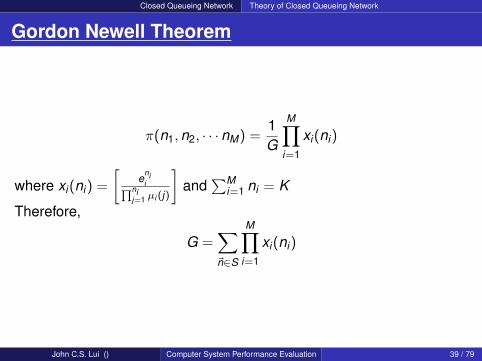
Gordon Newell Theorem

π(n1,n2, · · · nM) =1G

M∏i=1

xi(ni)

where xi(ni) =

[e

niiQni

j=1 µi (j)

]and

∑Mi=1 ni = K

Therefore,

G =∑~n∈S

M∏i=1

xi(ni)


Closed Queueing Network Computation Methods

Computation of G (assume SSFR)

Define S(m,n) = {(n1, · · · nm) | ni ≥ 0,∑m

i=1 ni = n}

G(m,n) =∑

~n∈S(m,n)

m∏i=1

xi(ni) where xi =ei

µi

G(m,n) =∑

~n∈S(m,n);

nm=0

m∏i=1

xnii +

∑~n∈S(m,n);

nm>φ

m∏i=1

xnii

=∑

~n∈S(m−1,n)

m−1∏i=1

xi(ni) + xm∑

~n∈S(m,n);

ki =ni (i 6=m);

km=nm−1

m∏i=1

xi(ki)

G(m,n) = G(m − 1,n) + xmG(m,n − 1) m,n > φ



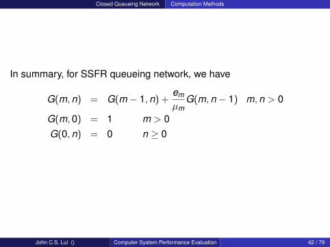
In summary, for SSFR queueing network, we have

G(m,n) = G(m − 1,n) +em

µmG(m,n − 1) m,n > 0

G(m,0) = 1 m > 0G(0,n) = 0 n ≥ 0



mn 0 1 2 3 i M-1 M

0 1 1 1 1 1

0e1µ1

e1µ1+e2µ2

e1µ1( )2

..........

..........

0

0

1

2

K-1

K

0

0

e1µ1( )K-1

e1µ1( )K

.......... ei

µix+

+

..........



Performance Measures

Idle Probability for node i :

P(NM = 0) =1

G(M,K )

∑~n∈S(M,K );

nM =0

M−1∏i=1

(ei

µi

)ni

=G(M − 1,K )

G(M,K )

Another way to express it:

P(Ni = 0) =1

G(M,K )

∑~n∈S(µ,k);

ni =0

i−1∏j=1

(ei

µj

)nj M∏k=i+1

(ek

µk

)nk

=G(M\i ,K )

G(M,K )



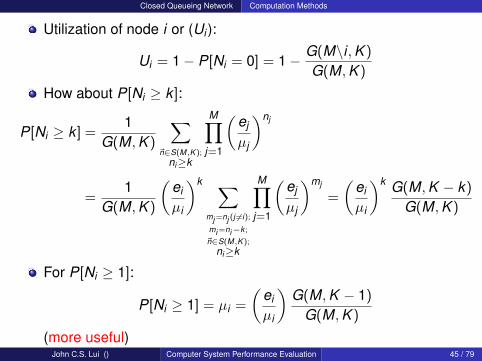
Utilization of node i or (Ui ):

Ui = 1− P[Ni = 0] = 1− G(M\i ,K )

G(M,K )

How about P[Ni ≥ k ]:

P[Ni ≥ k ] =1

G(M,K )

∑~n∈S(M,K );

ni≥k

M∏j=1

(ej

µj

)nj

=1

G(M,K )

(ei

µi

)k ∑mj =nj (j 6=i);

mi =ni−k ;

~n∈S(M,K );

ni≥k

M∏j=1

(ej

µj

)mj

=

(ei

µi

)k G(M,K − k)

G(M,K )

For P[Ni ≥ 1]:

P[Ni ≥ 1] = µi =

(ei

µi

)G(M,K − 1)

G(M,K )

(more useful)John C.S. Lui () Computer System Performance Evaluation 45 / 79


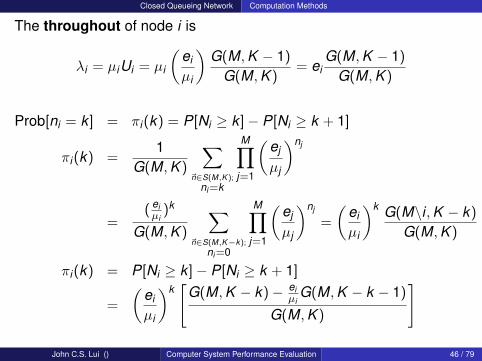
The throughout of node i is

λi = µiUi = µi

(ei

µi

)G(M,K − 1)

G(M,K )= ei

G(M,K − 1)

G(M,K )

Prob[ni = k ] = πi(k) = P[Ni ≥ k ]− P[Ni ≥ k + 1]

πi(k) =1

G(M,K )

∑~n∈S(M,K );

ni =k

M∏j=1

(ej

µj

)nj

=( eiµi

)k

G(M,K )

∑~n∈S(M,K−k);

ni =0

M∏j=1

(ej

µj

)nj

=

(ei

µi

)k G(M\i ,K − k)

G(M,K )

πi(k) = P[Ni ≥ k ]− P[Ni ≥ k + 1]

=

(ei

µi

)k[

G(M,K − k)− eiµi

G(M,K − k − 1)

G(M,K )

]



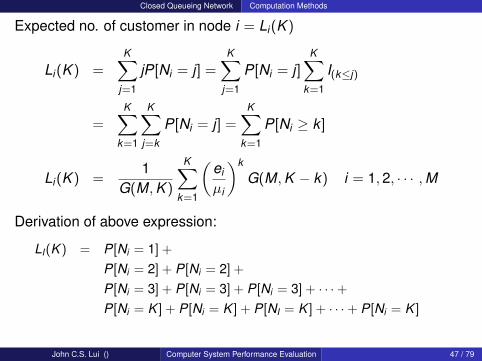
Expected no. of customer in node i = Li(K )

Li(K ) =K∑

j=1

jP[Ni = j] =K∑

j=1

P[Ni = j]K∑

k=1

I(k≤j)

=K∑

k=1

K∑j=k

P[Ni = j] =K∑

k=1

P[Ni ≥ k ]

Li(K ) =1

G(M,K )

K∑k=1

(ei

µi

)k

G(M,K − k) i = 1,2, · · · ,M

Derivation of above expression:

LI(K ) = P[Ni = 1] +

P[Ni = 2] + P[Ni = 2] +

P[Ni = 3] + P[Ni = 3] + P[Ni = 3] + · · ·+P[Ni = K ] + P[Ni = K ] + P[NI = K ] + · · ·+ P[Ni = K ]


Closed Queueing Network Convolution Algorithm

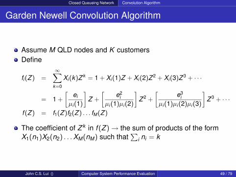
Garden Newell Convolution Algorithm

Assume M QLD nodes and K customersDefine

fi (Z ) =∞∑

k=0

Xi (k)Z k = 1 + Xi (1)Z + Xi (2)Z 2 + Xi (3)Z 3 + · · ·

= 1 +

[ei

µi (1)

]Z +

[e2

iµi (1)µi (2)

]Z 2 +

[e3

iµi (1)µi (2)µi (3)

]Z 3 + · · ·

f (Z ) = f1(Z )f2(Z ) . . . fM(Z )

The coefficient of Z k in f (Z )→ the sum of products of the formX1(n1)X2(n2) . . .XM(nM) such that

∑i ni = k



Thus

f (Z ) = 1+G(M,1)Z +G(M,2)Z 2+G(M,3)Z 3+· · ·+G(M, k)Z k +· · ·

*IDEA: build up f (Z ) from partial products gi(Z ) so that G(i , k) isthe coefficient of Z k in gi(Z )

g1(Z ) = f1(Z )

gi(Z ) = gi−1(Z )fi(Z ) i = 2,3, · · · ,M



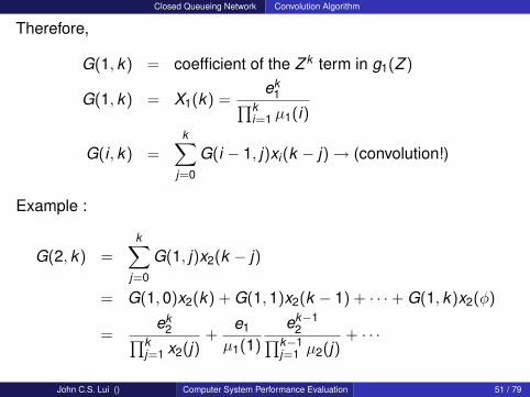
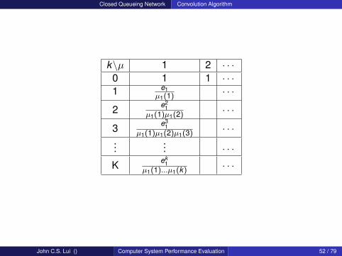
Therefore,

G(1, k) = coefficient of the Z k term in g1(Z )

G(1, k) = X1(k) =ek

1∏ki=1 µ1(i)

G(i , k) =k∑

j=0

G(i − 1, j)xi(k − j)→ (convolution!)

Example :

G(2, k) =k∑

j=0

G(1, j)x2(k − j)

= G(1,0)x2(k) + G(1,1)x2(k − 1) + · · ·+ G(1, k)x2(φ)

=ek

2∏kj=1 x2(j)

+e1

µ1(1)

ek−12∏k−1

j=1 µ2(j)+ · · ·



k\µ 1 2 · · ·0 1 1 · · ·1 e1

µ1(1) · · ·

2 e21

µ1(1)µ1(2) · · ·

3 e31

µ1(1)µ1(2)µ1(3) · · ·...

... · · ·K ek

1µ1(1)...µ1(k) · · ·



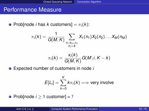
Performance Measure

Prob[node i has k customers] = πi(k):

πi(k) =1

G(M,K )

∑~n∈S(µ,k);

ni =k

X1(n1)X2(n2) . . .XM(nM)

πi(k) =xi(k)

G(M,K )G(M\i ,K − k)

Expected number of customers in node i

E [Li ] =K∑

k=0

kπi(k) =⇒ very involve

Prob[node i ≥ 1 customer] = ?



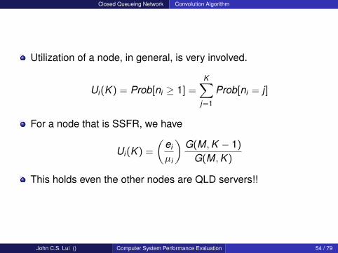
Utilization of a node, in general, is very involved.

Ui(K ) = Prob[ni ≥ 1] =K∑

j=1

Prob[ni = j]

For a node that is SSFR, we have

Ui(K ) =

(ei

µi

)G(M,K − 1)

G(M,K )

This holds even the other nodes are QLD servers!!



Example :

......

front end communication

transaction processing

query processing

0P

1P

2P

3P

4P

terminal

!"

!average think time = 1/

eT = eF p0; eF = eT + eCp2; eC = eF p1 + eD + eP ;eD = eCp3; eP = eCp4

eT = 1; eF = 1p0

; eC = 1−p0p0p2

; eD = (1−p0)p3p0p2

; eP = (1−p4)p4p0p2

ρT = eTλ = 1

λ ; ρF = 1p0µF

; ρC = (1−p0)p0p1µc

; ρD = (1−p0)p3p0p2µ0

ρP = (1−p0)p4p0p2µp

π(nT ,nF ,nC ,nD,np) =1G

(ρT )nT

nT !(ρF )nF (ρC)nC (ρD)nD (ρP)nP



UF = ?

Since UF is a SSFR, we have

UF = ρFG(5,K − 1)

G(5,K )=

1p0µF

G(5,K − 1)

G(5,K )

Average throughput or rate of request completion is:

λ∗ = µF p0UF =G(5, k − 1)

G(5, k)

but Little’s Result (N = λT )T = the expected response time = K

λ∗ = KG(5,k)G(5,K−1)

T = average think + average processing time = KG(5,k)G(5,K−1)

T = 1λ + average processing time = KG(5,k)

G(5,K−1)

Therefore, average processing time = KG(5,k)G(5,K−1) −

1λ


Closed Queueing Network Multiclass Queueing Networks

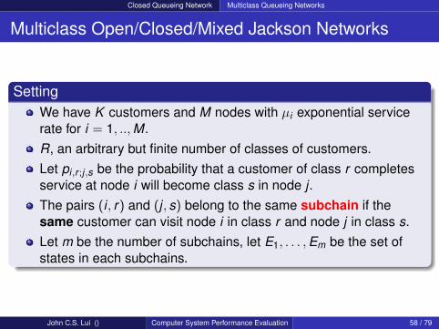
Multiclass Open/Closed/Mixed Jackson Networks

SettingWe have K customers and M nodes with µi exponential servicerate for i = 1, ..,M.R, an arbitrary but finite number of classes of customers.Let pi,r ;j,s be the probability that a customer of class r completesservice at node i will become class s in node j .The pairs (i , r) and (j , s) belong to the same subchain if thesame customer can visit node i in class r and node j in class s.Let m be the number of subchains, let E1, . . . ,Em be the set ofstates in each subchains.



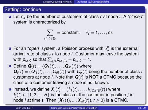
Setting: continueLet nir be the number of customers of class r at node i . A “closed”system is characterized by∑

(i,r)∈Ej

= constant. ∀j = 1, . . . ,m.

For an “open” system, a Poisson process with λ0ir is the external

arrival rate of class r to node i . Customer may leave the systemwith pi,r ;0 so that

∑j,s pi,r ;j,s + pi,r ;0 = 1.

Define Q(t) = (Q1(t), . . . ,QM(t)) whereQi(t) = (Qi1(t), . . . ,QiR(t)) with Qir (t) being the number of class rcustomers at node i . Note that Q(t) is NOT a CTMC because theclass of a customer leaving a node is not known.Instead, we define X i(t) = (Ii1(t), . . . , Ii,|Qi (t)|(t)) whereIij(t) ∈ {1,2, ...,R} is the class of the customer in position j innode i at time t . Then (X 1(t), ...,X M(t)), t ≥ 0) is a CTMC.



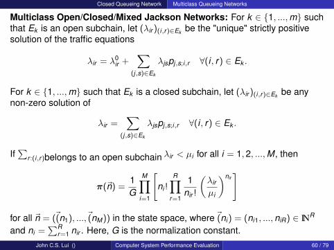
Multiclass Open/Closed/Mixed Jackson Networks: For k ∈ {1, ...,m} suchthat Ek is an open subchain, let (λir )(i,r)∈Ek be the "unique" strictly positivesolution of the traffic equations

λir = λ0ir +

∑(j,s)∈Ek

λjspj,s;i,r ∀(i , r) ∈ Ek .

For k ∈ {1, ...,m} such that Ek is a closed subchain, let (λir )(i,r)∈Ek be anynon-zero solution of

λir =∑

(j,s)∈Ek

λjspj,s;i,r ∀(i , r) ∈ Ek .

If∑

r :(i,r)belongs to an open subchain λir < µi for all i = 1,2, ...,M, then

π(~n) =1G

M∏i=1

[ni !

R∏r=1

1nir !

(λir

µi

)nir]

for all ~n = (~(n1), ...,~(nM)) in the state space, where~(ni ) = (ni1, ...,niR) ∈ INR

and ni =∑R

r=1 nir . Here, G is the normalization constant.John C.S. Lui () Computer System Performance Evaluation 60 / 79


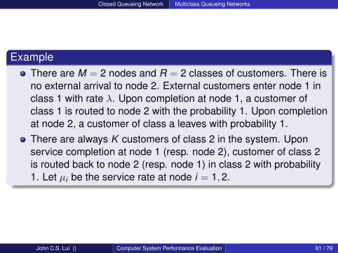
ExampleThere are M = 2 nodes and R = 2 classes of customers. There isno external arrival to node 2. External customers enter node 1 inclass 1 with rate λ. Upon completion at node 1, a customer ofclass 1 is routed to node 2 with the probability 1. Upon completionat node 2, a customer of class a leaves with probability 1.There are always K customers of class 2 in the system. Uponservice completion at node 1 (resp. node 2), customer of class 2is routed back to node 2 (resp. node 1) in class 2 with probability1. Let µi be the service rate at node i = 1,2.



Example: continueThe state space S is

S = {(n11,n12,n21,n22) ∈ IN4 : n11 ≥ 0,n21 ≥ 0,n12 + n22 = K}.

There are two subchains: E1 (open), and E2 (closed), withE1 = {(1,1), (2,1)} and E2 = {(1,2), (2,2)}.

We find λ11 = λ2,1 = λ and λ12 = λ22. Take λ12 = λ22 = 1 for instance.We have

π(~n) =1G

(n1

n11

)(n2

n22

)(λ

µ1

)n11(λ

µ2

)n21(

1µ1

)n12(

1µ2

)n22

with λ < µi , i = 1,2 (stability condition).



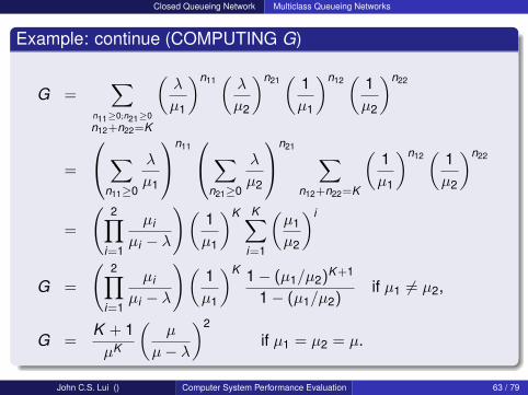
Example: continue (COMPUTING G)

G =∑

n11≥0;n21≥0n12+n22=K

(λ

µ1

)n11(λ

µ2

)n21(

1µ1

)n12(

1µ2

)n22

=

∑n11≥0

λ

µ1

n11∑

n21≥0

λ

µ2

n21 ∑n12+n22=K

(1µ1

)n12(

1µ2

)n22

=

(2∏

i=1

µi

µi − λ

)(1µ1

)K K∑i=1

(µ1

µ2

)i

G =

(2∏

i=1

µi

µi − λ

)(1µ1

)K 1− (µ1/µ2)K +1

1− (µ1/µ2)if µ1 6= µ2,

G =K + 1µK

(µ

µ− λ

)2

if µ1 = µ2 = µ.



Extension to M/M/cLet ci ≥ 1 be the number of servers at node i and defineαi(j) = min(ci , j) for i = 1, ...,M. Hence µiαi(j) is the service rate atnode i when there are j customers. We have

π(~n) =1G

M∏i=1

ni∏j=1

1αi(j)

ni !

(R∏

r=1

1nir !

(λir

µi

)nir) .



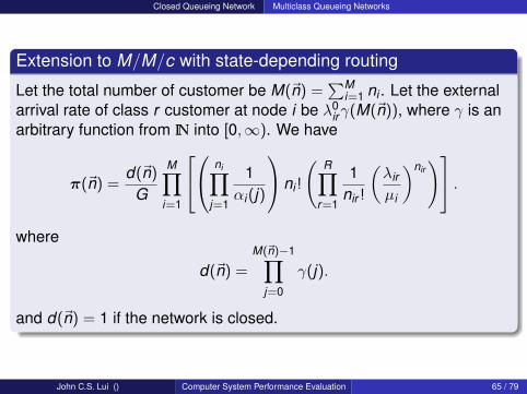
Extension to M/M/c with state-depending routing

Let the total number of customer be M(~n) =∑M

i=1 ni . Let the externalarrival rate of class r customer at node i be λ0

irγ(M(~n)), where γ is anarbitrary function from IN into [0,∞). We have

π(~n) =d(~n)

G

M∏i=1

ni∏j=1

1αi(j)

ni !

(R∏

r=1

1nir !

(λir

µi

)nir) .

where

d(~n) =

M(~n)−1∏j=0

γ(j).

and d(~n) = 1 if the network is closed.


Closed Queueing Network BCMP Networks

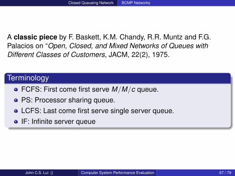
A classic piece by F. Baskett, K.M. Chandy, R.R. Muntz and F.G.Palacios on “Open, Closed, and Mixed Networks of Queues withDifferent Classes of Customers, JACM, 22(2), 1975.

TerminologyFCFS: First come first serve M/M/c queue.PS: Processor sharing queue.LCFS: Last come first serve single server queue.IF: Infinite server queue



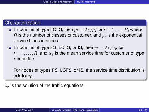
CharacterizationIf node i is of type FCFS, then ρir = λir/µi for r = 1, . . . ,R, whereR is the number of classes of customer, and µi is the exponentialservice times in node i .If node i is of type PS, LCFS, or IS, then ρir = λir/µir forr = 1, . . . ,R, and µir is the mean service time for customer of typer in node i .

For nodes of types PS, LCFS, or IS, the service time distribution isarbitrary.

λir is the solution of the traffic equations.



TheoremFor a BCMP network with M nodes and R classes of customer, whichis open, closed, or mixed in which each node is of type FCFS, PS,LCFS, or IS, the steady state probabilities are:

π(~n) =d(~n)

G

M∏i=1

fi(~ni).

where ~n = (~n1, · · · , ~nM) in the state space S with~ni = (ni1,ni2, · · · ,niR) where nir is the number of jobs of class r atnode i. Moreover, |~ni | =

∑Rr=1 nir for i = 1,2, . . . ,M.

G <∞ is the normalization constant such that∑~n∈S π(~n) = 1,

d(~n) =∏M(~n)−1

j=0 γ(j) if the arrivals depend on the total number of

customers M(~n) =∑M

i=1 |~ni |, and d(~n) = 1 if the network is closed.



fi(~ni) for different types of nodesIf node i is of type FCFS:

fi(~ni) = |~ni |!|~ni |∏j=1

1αi(j)

R∏r=1

ρnirir

nir !

If node i is of type PS or LCFS:

fi(~ni) = |~ni |!R∏

r=1

ρnirir

nir !

If node i is of type IS:

fi(~ni) =R∏

r=1

ρnirir

nir !



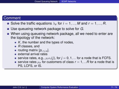
CommentSolve the traffic equations λir for i = 1, ...,M and r = 1, ...,R.Use queueing network package to solve for G.When using queueing network package, all we need to enter arethe topology of the network:

K , the number and the types of nodes,R classes, androuting matrix [pi,r ;j,s].external arrival ratesservice rates, e.g., µiαi (j), for j = 0,1, ... for a node that is FCFS.service rates µir for customers of class r = 1, ...R for a node that isPS, LCFS, or IS.


Closed Queueing Network Mean Value Analysis (MVA)

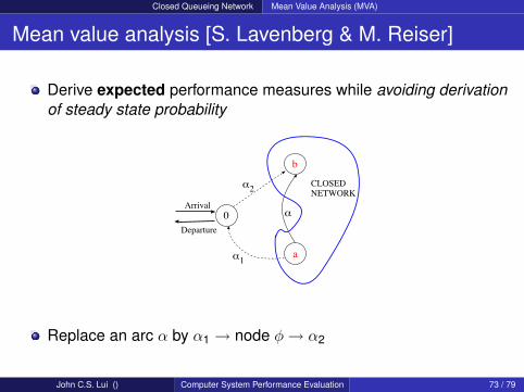
Mean value analysis [S. Lavenberg & M. Reiser]

Derive expected performance measures while avoiding derivationof steady state probability

0

b

a!

!

1

!2 CLOSEDNETWORK

Arrival

Departure

Replace an arc α by α1 → node φ→ α2



Whenever a customer arrives at node φ (via along α1), it departsfrom the network and is replaced by a"stochastically" identical customer who has the same routingprobability along arc α2

This open network behaves exactly as the closed one (exceptnode φ)



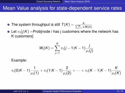
Mean Value analysis for state-dependent service rates

The system throughput is still T (K ) = KPMi=1 vi Wi (k)

Let πi(j |K ) =Prob[node i has j customers where the network hasK customers]

Wi(K ) =K∑

j=1

πi(j − 1|K − 1)j

µi(j)

Example:

πi(0|K − 1)1

µi(1)+ πi(1|K − 1)

2µi(2)

+ · · ·+ πi(K − 1|K − 1)K

µi(K )



The mean queue length is:

Li(K ) =K∑

j=1

jπi(j |K )

By definition,πi(0|0) = 1 and

πi(j |K ) =

{vi T (K )µi (j) πi(j − 1|K − 1) j = 1,2, . . . , k1−

∑Kk=1 πi(k |K ) j = φ



For the α we chosen, let us define the network throughput T asthe average rate customers pass along arc α in steady state.Now we can view T as the external arrival rate (γ) in the opennetwork.Suppose that we have M nodes in the network. Define

vi = average number of visit to node i by a customer= (visitation rate)

λi = average arrival rate of customer to node i

λi = Tvi , v0 = vaqab

But since customers visit node φ EXACTLY ONCE, v0 = 1,therefore:

va =1

qab; vj =

µ∑i=1

viqij

Once one vi is found,we can find other vi ’s.



Looking at node i, let Li= average no. of customers, we have:

Li = λiwi , Li = Tviwi

But since∑M

i=1 Li = K = T∑M

i=1 viwi , therefore the systemthroughput

T =K∑M

i=1 viwi

If node i is infinite server,then

wi =1µi

If node i is single server fixed rate (SSFR),

wi =1µi

[Yi + 1]

where Yi is the mean number of customers seen by an arrival tonode i.



Example:

πi(j |K ) =

{vi T (K )µi (j) πi(j − 1|K − 1) j = 1,2, . . . , k1−

∑Kk=1 πi(k |K ) j = φ

Assume it is node 1 (that is , i=1)

π1(1|1) =v1T (1)

µ1(1)π1(φ|φ) =

v1T (1)

µ1(1)

π1(φ|1) = 1− π1(1|1)

π1(1|2) =v1T (2)

µ1(1)π1(φ|1)

π1(2|2) =v1T (2)

µ2(2)π1(1|1)

π1(φ|2) = 1− π(1|2)− π(2|2)


Documents

Introduction to Queueing Networkscslui/CSC5420/queueing_network_beamer.pdf · Introduction to Queueing Networks ... Theory on Jackson Networks Examples 3 Closed Queueing Network Example