Queueing Systems07

8/2/2019 Queueing Systems07

http://slidepdf.com/reader/full/queueing-systems07 1/23

Priority queueing systems: from probability generating functions

to tail probabilities

Tom Maertens∗, Joris Walraevens, Herwig BruneelGhent University – UGent

Department of Telecommunications and Information ProcessingSMACS Research Group

Sint-Pietersnieuwstraat 41, B-9000 Gent, BelgiumPhone: +32-9-2648901

Fax: +32-9-2644295E-mail: {tmaerten,jw,hb}@telin.UGent.be

Abstract

Obtaining (tail) probabilities from a transform function is an important topic in queueing theory. Toobtain these probabilities in discrete-time queueing systems, we have to invert probability generatingfunctions, since most important distributions in discrete-time queueing systems can be determined in theform of probability generating functions. In this paper, we calculate the tail probabilities of two particularrandom variables in discrete-time priority queueing systems, by means of the dominant singularity ap-proximation. We show that obtaining these tail probabilities can be a complex task, and that the obtainedtail probabilities are not necessarily exponential (as in most ’traditional’ queueing systems). Further, weshow the impact and significance of the various system parameters on the type of tail behavior. Finally,we compare our approximation results with simulations.

keywords priority queueing systems, tail probabilities, dominant pole, non-exponential behavior

1 Introduction

Many probability distributions of interest in queueing models can be determined in the form of trans-

forms: the Laplace-Stieltjes transforms of continuous density functions or the z-transforms of discrete

probability mass functions. The benefit of using transforms in analyses with stochastic variables has been

frequently demonstrated in the past. Transforms are furthermore very useful to extract numerical results,e.g., to calculate moments. However, a seeming disadvantage of working with transforms is that it is not

always easy to explicitly calculate the corresponding cumulative distribution functions (cdf’s), probability

density functions (pdf), or probability mass functions (pmf’s).

Often, we are only interested in the tail of the probability distribution. Tail probabilities typically

represent the ’exceptional’ situations in a queueing system (or more generally, a communication network),

of which we want to estimate the frequency of. E.g. the probability that the delay is larger than a given

∗Corresponding author

1



value N or the packet loss are examples of interesting performance measures for which the calculation

of the (asymptotic behavior of) tail probabilities is usually sufficient. Obtaining tail probabilities of a

stochastic variable from its transform, which is basically an inversion problem, is thus an important

topic in queueing theory. A theoretical solution method is to analytically invert the transform, yielding an

explicit , closed-form expression for the underlying probability distribution. However, this is only possible if

the transform expressions are simple enough. In sophisticated queueing models, this method is practically

infeasible. Therefore, one has to look for approximate solutions.

From our point of view, existing approximate inversion techniques can be roughly divided into two

categories: numerical inversion methods and analytical inversion methods. Abate and Whitt [4] provide an

extensive study of various numerical methods for transform inversion. In general, theoretical solutions for

the inversion problem can usually be expressed via integrals (see e.g. [9] for a short review): a line integral

in the continuous case or a contour integral in the discrete case. These basic inversion integrals can then

be calculated by performing a numerical integration. The Fourier-series method numerically integrates a

standard inversion integral by means of the trapezoidal rule (see e.g. [4]). In [7] (Laplace transforms) and

[5] (probability generating functions), the authors propose Poisson summation formulas which identify the

discretization errors associated with this trapezoidal rule. Algorithms based on the Fourier-series method

are further a.o. presented in [19] and [21]. Most of these algorithms require the evaluation of the involved

transforms at many complex numbers. However, if the transform is only characterised implicitly via a

functional equation (e.g., the busy-period distribution in a GI/GI/1 system), it may be quite involved

to obtain these values. Abate and Whitt [6] discuss the solution of functional equations for complexarguments, and provide conditions for iterative methods to converge. Variants of these methods can

a.o. be found in [9] and [13]. Note finally that the Fourier-series method is closely related to the Laguerre

method (see e.g. [2, 3, 16]), i.e., the desired function is in both methods represented as an expansion in

terms of orthogonal functions, where the coefficients are expressed in terms of the transform.

A second class of approximate inversion techniques exists of analytical methods, which all more or less

follow a similar procedure. After determining the (asymptotic) tail behavior, one calculates the correspond-

ing parameters. Finally, approximate expressions for the tail probabilities are derived. The asymptotic

tail behavior of a probability distribution can be obtained analytically by calculating the value and type

of the rightmost singularity of the Laplace transform in the continuous case (see e.g. [8]), or by deter-

mining the value and type of the singularity with the smallest modulus of the pgf in the discrete case

(see e.g. [10]). Choudhury and Lucantoni [11] showed further that high-order moments of the stochastic

variable can be used to estimate the asymptotic parameters of the cdf. Abate et al [1] provide theoret-

ical support for this moment-based algorithm, and present new refined estimators which converge much

faster than the estimators proposed in [11]. The techniques in [1] were also used in [22] for computing

2



the asymptotic parameters numerically. When the transforms are not available explicitly, as in models of

busy-periods or polling systems, moment-based algorithms prove useful (see e.g. [12]). Finally, when the

transforms are only available in matrix-form, one can use an analytical method based on the dominant

eigenvalue of the transform-matrix and on the Chernoff large deviations approximation (see e.g. [15]).

In summary, in the analytical approach, an approximate expression is found in terms of a limited

number of parameters (such as the dominant singularity of the pgf), while the numerical approach only

yield ’a set of numbers’. The analytical method has the advantage that the behavior of the pmf is found. On

the other hand, numerical inversion techniques are usually more accurate for low arguments of the cdf’s

or pmf’s. The analytical approach thus complements the numerical one.

In this paper, we use the dominant singularity method for deriving approximate expressions for tail

probabilities of a discrete-time variable from its pgf. E.g. Bruneel et al [10] have shown that for high n, the

pmf x(n) of a discrete variable X is dominated by the contribution of the singularity of the corresponding

pgf, with the smallest absolute value. This dominant singularity is necessarily positive real and larger

than 1. In traditional single-class queueing systems with a FIFO scheduling discipline, the pgf’s of the

system quantities generally have one type of dominant singularity, usually a simple pole (i.e., a zero of

the denominator of the pgf with multiplicity 1) (see e.g. [10]). This leads to the well-known geometric (or

exponential) behavior x(n) ≈ Ks−n−1∗

, with s∗ the dominant pole of the corresponding pgf.

In e.g. priority queueing systems however, several (types of) singularities may play a role (see e.g. [8, 17,

26]). In [17] and [26], the authors analyse “basic” discrete-time priority queueing systems: two-class queues

with single-slot service times and with a HOL (Head-Of-the-Line) priority scheduling discipline. E.g. in[26], it is shown that two (types of) singularities on the positive real axis of the pgf of the low-priority

packet delay in such a priority system play a role: a simple pole and a branch point. This branch point

is a result of an implicitly defined function appearing in the pgf. Both singularities can dominate and

it depends on the system parameters (arrival rates in that case) which one is dominant. A consequence

of the appearance of two types of singularities is that two forms of tail behavior can distinguished be,

namely exponential behavior when the simple pole dominates and non-exponential tail behavior when

the branch point dominates. Tail behavior in continuous-time priority systems has been examined, via

analytical methods in e.g. [1, 8, 11, 22], or via numerical methods in e.g. [23]. We finally note that the

papers mentioned in this paragraph all assume infinite queue sizes. Different results are however obtained

by scaling the number of arrival sources along with the capacity of the system and the queue size (see

e.g. [20]).

In this paper, we calculate the tail probabilities of two particular random variables in more complex

discrete-time priority queueing systems, whereby more than two (types of) singularities may exist and

each of them may (co-)dominate, depending on the values of the various system parameters. We derive

3



expressions for the tail probabilities using the dominant singularity approximation, and we compare

our approximations with simulations to validate the used method. The contribution of this paper thus

mainly concerns the solution technique that is used, and the extension of this solution technique to rather

complicated queueing systems. Hence, also the generated results are a major contribution of the current

paper. Specifically, we show that the tail behavior in priority queueing systems can be quite complicated

and diverse, highly depending on the values of the system parameters (e.g. arrival and service rates).

The outline of the paper is as follows. In the following section, we describe the tail behavior and derive

expressions for the tail probabilities of the system contents of a complex HOL (Head-Of-Line) priority

queue. In section 3, we sketch the tail behavior of the delay of a low-priority packet in a HOL-PJ (HOL

with Priority Jumps) queue. Some conclusions are drawn in section 4.

2 The total system contents of a HOL priority queue

2.1 Preliminaries

We first concentrate on the total, steady-state system contents of a single-server, two-class priority

queueing system with the number of per-slot class-1 and class-2 arrivals characterised by the joint pgf

A(z1, z2) and the marginal pgf’s AT (z) = A(z, z), A1(z) = A(z, 1) and A2(z) = A(1, z) (with λj = A

j(1)

the arrival rate of class j). The waiting room is of infinite capacity and the service times are generally

distributed (with S j(z) the pgf of the service times of class j packets and µj = S j(1) the mean service

time of a class j packet). Arriving packets are scheduled according to a HOL non-preemptive priority

scheduling discipline, where class-1 packets are assumed to have priority over class-2 packets. The pgf of

the total system contents has been derived in [25], and is given by

U T (z) =

(1− ρT )(z − 1)

S 1(AT (z))(AT (z)− 1)(z − S 2(A(Y (z), z)))

+z (A(Y (z), z)− 1)(S 2(AT (z))− S 1(AT (z)))

(z − S 1(AT (z)))(z − S 2(A(Y (z), z)))(AT (z)− 1), (1)

where ρT ρ1 + ρ2 = λ1µ1 + λ2µ2 denotes the total load, and where Y (z) is the only solution of

x−S 1(A(x, z)) = 0 with |x| < 1 and |z| < 1. The pgf Y (z) is thus implicitly defined as S 1(A(Y (z), z)). Note

that the total load has to be smaller than 1 (i.e., ρT < 1) to ensure having a stable system and proper

steady-state system distributions. We furthermore assume in the remainder that the pgf’s AT (z), Aj(z)

and S j(z) ( j = 1, 2) and their derivatives go to infinity for z equal to their radii of convergence, or for

z →∞. This includes all ’usual’ arrival and service processes, except e.g. processes with a long tail. For

the numerical examples and figures in this section, we use a two-dimensional binomial arrival process,

with joint pgf A(z1, z2) = (1 − λ1(1 − z1)/N − λ2(1 − z2)/N )N (with N = 16), and deterministic or

4



0

1

2

3

4

5

6

7

0 0.5 1 1.5 2 2.5 3

zsB

x

Y(z)

Y*(z)

Figure 1: Solutions of x− S 1(A(x, z)) = 0

geometric service times, with pgf’s S j(z) = zµj or S j(z) =z

z − µj(z − 1)respectively. It should be noted

that the figures serve only as an illustration to show that the values of the system parameters play a role

in the existence - and thus also in the dominance - of the possible singularities. The derivations in the

paper are thus valid for other arrival and service processes as well.

It is obvious that the calculation of the tail probabilities of the total system contents is not straight-

forward, since it is not a priori clear from expression (1) which singularity of U T (z) is dominant. Sev-

eral singularities may play a role, namely the dominant positive real (> 1) zeros of z − S 1(AT (z)) and

z−S 2(A(Y (z), z)), denoted by sT and sL respectively, and the radii of convergence of the pgf’s in expres-

sion (1). Furthermore, the tail behavior of the total system contents is also influenced by the dominant

singularity of the function Y (z), denoted by sB in the remainder. We first take a closer look at this

function on the positive real axis.

2.2 Singularity sB

First we note that Y (z) is convex on the positive real axis, since Y (z) is a pgf of a stochastic variable

(see [24] for a proof). As z increases along the positive real axis, a branch point sB will be encountered in

Y (z) where Y (z) →∞ (see e.g. [17] for a similar case). For values of z beyond that point, Y (z) is no longer

properly defined (or, in other words, x− S 1(A(x, z)) = 0 has no solution for z > sB). However, a second

real and positive solution Y ∗(z) of the functional equation x

−S 1(A(x, z)) = 0 for positive real z, exists and

decreases as z increases (see Figure 1). E.g. for z = 1, it is easily seen that x− S 1(A1(x)) has 2 distinct

zeros (i.e., Y (1) = 1 and Y ∗(1) > 1), since S 1(A1(x)) is convex anddS 1(A1(x))

dx

x=1

= ρ1 < 1. Both

solutions coincide for z = sB. sB is the solution of

Y (sB) = S 1(A(Y (sB), sB))

Y (sB) →∞⇒ Y (sB)− S 1(A(Y (sB), sB)) = 0

S 1(A(Y (sB), sB))A(1)(Y (sB), sB) = 1. (2)

5



0

2

4

6

8

10

0 1 2 3 4 5

z

x

sT

Y(z)

Y*(z)

z

S1(AT(z))

0

1

2

3

4

5

6

7

0 2 4 6 8 10 12 14 16 18

z

x

sT

Y(z)

Y*(z)

z

S1(AT(z))

a. sT = Y (sT ) b. sT = Y ∗(sT )

Figure 2: The singularity sT

with A(1)(z1, z2) ∂A(z1, z2)

∂z1. Remark that Y (sB) is infinite, but that Y (sB) remains finite. Applying

the results of [14], one can show that in the neighbourhood of sB , Y (z) is approximately given by

Y (z) ≈ Y (sB)−K Y (sB − z)1/2, (3)

with

K Y =

2A(2)(Y (sB), sB)

S 1 (A(Y (sB), sB))(A(1)(Y (sB), sB))3 + A(11)(Y (sB), sB)), (4)

where A(2)(z1, z2) ∂A(z1, z2)

∂z2

and A(11)(z1, z2) ∂ 2A(z1, z2)

∂z2

1

. Expression (4) is found by taking the

limit z → sB in expression (3), and by using the definition of Y (z). Since Y (z) appears in the expression

of U T (z), sB is also a singularity of U T (z), and thus plays a role in the tail behavior of the total system

contents.

2.3 Singularity sT

A second potential singularity sT of U T (z) on the positive real axis (> 1) is given by the zero of

z − S 1(AT (z)). We will show that sT is however not in all cases a singularity of U T (z). Since sT is a

zero of z − S 1(A(z, z)), it is easily seen that (x, z) = (sT , sT ) is a solution of x− S 1(A(x, z)) = 0. As a

consequence, sT has to be smaller than sB, since this equation has no solution for z > sB (see previous

subsection). Furthermore, we have shown in the previous paragraph that the equation x−S 1(A(x, z)) = 0

has 2 positive real solutions - namely (Y (z), z) and (Y ∗(z), z) - for z < sB positive real. Therefore,

sT = Y (sT ) or sT = Y ∗(sT ), depending on the pgf S 1(AT (z)). Both cases are illustrated in Figure 2,

where the functions Y (z), Y ∗(z), z and S 1(AT (z)) are shown. Note that sT = Y (sT ) if sT < Y (sB) and

sT = Y ∗(sT ) if sT > Y (sB), since Y (z) (Y ∗(z)) is maximal (minimal) in sB. It is now easily verified that

in the case that sT = Y (sT ), sT is also a zero of the numerator of U T (z) (see expression (1)) and that it

6



0

1

2

3

4

5

6

0 1 2 3 4 5 6 7 8

z

x

sL

Y(z)

z-S2(A(x,z))=0

0

1

2

3

4

5

6

0 2 4 6 8 10 12 14 16 18

z

x

Y(z)

z-S2(A(x,z))=0

a. sL exists b. sL does not exist

Figure 3: The singularity sL

is thus not a singularity of U T (z). Note that in this case, it is possible that sT ≤ 1 (see subsection 2.5). If

sT = Y ∗(sT ) on the other hand, sT is not a zero of the numerator and is thus indeed a singularity of

U T (z).

So, summarizing, three cases are possible for sT : sT = Y (sT ) < Y (sB), sT = Y (sB) (in which case

the branch point sB and sT coincide, see further) and sT = Y ∗(sT ) > Y (sB). In the second and third

case, sT is a singularity, with multiplicity 1. Indeed, due to the convexity of S 1(AT (z)), z − S 1(AT (z))

has at most 2 positive real zeros. z = 1 is one of them and z = sT is the other. Since sT > 1 when sT is

a pole, both zeros have multiplicity 1.

2.4 Singularity sL

A third potential singularity sL of U T (z) is given by the (dominant) solution of z−S 2(A(Y (z), z)) = 0,

on the positive real axis (> 1). Since S 2(A(Y (z), z)) is a pgf, and thus a convex function for z positive real,

z−S 2(A(Y (z), z)) = 0 has at most 2 positive real solutions, i.e., z = 1 and z = sL, each with multiplicity

1. Note further that since Y (z) appears in this equation, and since Y (z) does not exist for z > sB, this

possible solution sL has to be smaller than sB. To characterise this solution sL, we first transform the

equation z − S 2(A(Y (z), z)) = 0 into the following system of equations:

z − S 2(A(x, z)) = 0x = Y (z)

. (5)

If this system has a solution for z > 1 on the real axis, it is (x, z) = (Y (sL), sL) (see Figure 3a.). However,

this system does not always have a solution, in which case sL does not exist. This can be seen in Figure

3b., where the function x = Y (z) does not cut the function z−S 2(A(x, z)) for x, z > 1. In summary, three

possible cases can occur for the potential singularity sL: sL exists and sL < sB, sL exists and sL = sB or

sL does not exist.

7



2.5 Radii of convergence

Until now, we have focused on the potential poles of the denominator and on the branch point of

the implicitly defined function Y (z). Thereby, we have (implicitly) assumed that all pgf’s appearing in

expression (1) are analytic in the region of these singularities, i.e., that the radii of convergence of these

pgf’s do not play a role as possible dominant singularities of U T (z). In this subsection, we will prove that

this is indeed the case for all pgf’s appearing in (1), except for one, namely S 2(AT (z)). First, we will show

that the radii of convergence of S 1(AT (z)), AT (z), S 2(A(Y (z), z)), A(Y (z), z) are necessarily larger than

at least one of the singularities sB, sL or sT .

We first focus on the radius of convergence of S 1(AT (z)). We distinguish two cases: sT is a singularity

or sT is not a singularity (see subsection 2.3). In the first case, sT is within the region of convergence of

S 1(AT (z)), since sT > 1 is a solution of z − S 1(AT (z)) = 0. In the second case, one can prove that |z| <

|Y (z)| for |z| larger than the largest zero of z−S 1(AT (z)) (i.e., 1 or sT ). For those z, |Y (z)| > |S 1(AT (z))|and as a result, Y (z) will reach its branch point sB before S 1(AT (z)) diverges. Concluding, the radius of

convergence of S 1(AT (z)) is in both cases preceded by another singularity of U T (z).

Further, it is easily verified that the radius of convergence of S 2(A(Y (z), z)) is not a new potential

singularity. Again two cases are distinguished: sL exists or sL does not exist (see subsection 2.4). In the

first case, S 2(A(Y (z), z)) < z for 1 < z < sL sincedS 2(A(Y (z), z))

dz

z=1

< 1, S 2(A(Y (sL), sL)) = sL,

and S 2(A(Y (z), z)) is a convex function. As a result, the radius of convergence of S 2(A(Y (z), z)) is larger

than sL. In the second case, S 2(A(Y (z), z)) < z for 1 < z < sB sincedS 2(A(Y (z), z))

dz z=1

< 1 and Y (z)

reaches its branch point before S 2(A(Y (z), z)) reaches z. As a result, sB is the radius of convergence of

S 2(A(Y (z), z)), and we have already treated this singularity in subsection 2.2.

Thirdly, since the service times have means bigger than or equal to 1, S 1(AT (z)) ≥ AT (z) and

S 2(A(Y (z), z)) ≥ A(Y (z), z), for z larger than 1 and positive real. As a result, the radii of convergence of

AT (z) and A(Y (z), z) are larger (or equal) than the radii of convergence of S 1(AT (z)) and S 2(A(Y (z), z))

respectively, and thus do not play a role (a fortiori) in the tail behavior of U T (z) (or do not yield new

potential singularities).

Finally, as already mentioned, the radius of convergence of S 2(AT (z)), denoted by sQ, can be the

dominant singularity of U T (z). The reason why this singularity can be dominant is that S 2(z) does not

influence the singularities sB and sT , as can be seen from subsections 2.2 and 2.3 respectively. Hence,

S 2(z) can be such that S 2(AT (z)) →∞ before z reaches sB or sT . Furthermore, S 2(z) can be such that

S 2(AT (z)) > S 2(A(Y (z), z)) for z > 1, and even so that for z increasing, S 2(AT (z)) reaches its radius of

convergence sQ before U T (z) reaches sL. As a result, sQ can be smaller than sB, sT and sL, and thus be

the dominant singularity of U T (z). We will give an example of such S 2(z) in the following subsection.

8



0

0.2

0.4

0.6

0.8

1

0 0.2 0.4 0.6 0.8 1

ρ1

ρ2

sL

sT

sT = Y(sB)

sL = sB

sL = sT

0

0.2

0.4

0.6

0.8

1

0 0.2 0.4 0.6 0.8 1

ρ1

ρ2sL

sB

sT

sT = Y(sB)

sL = sB

sL = sT

a. when µ1 = 2, µ2 = 4 b. when µ1 = 4, µ2 = 2

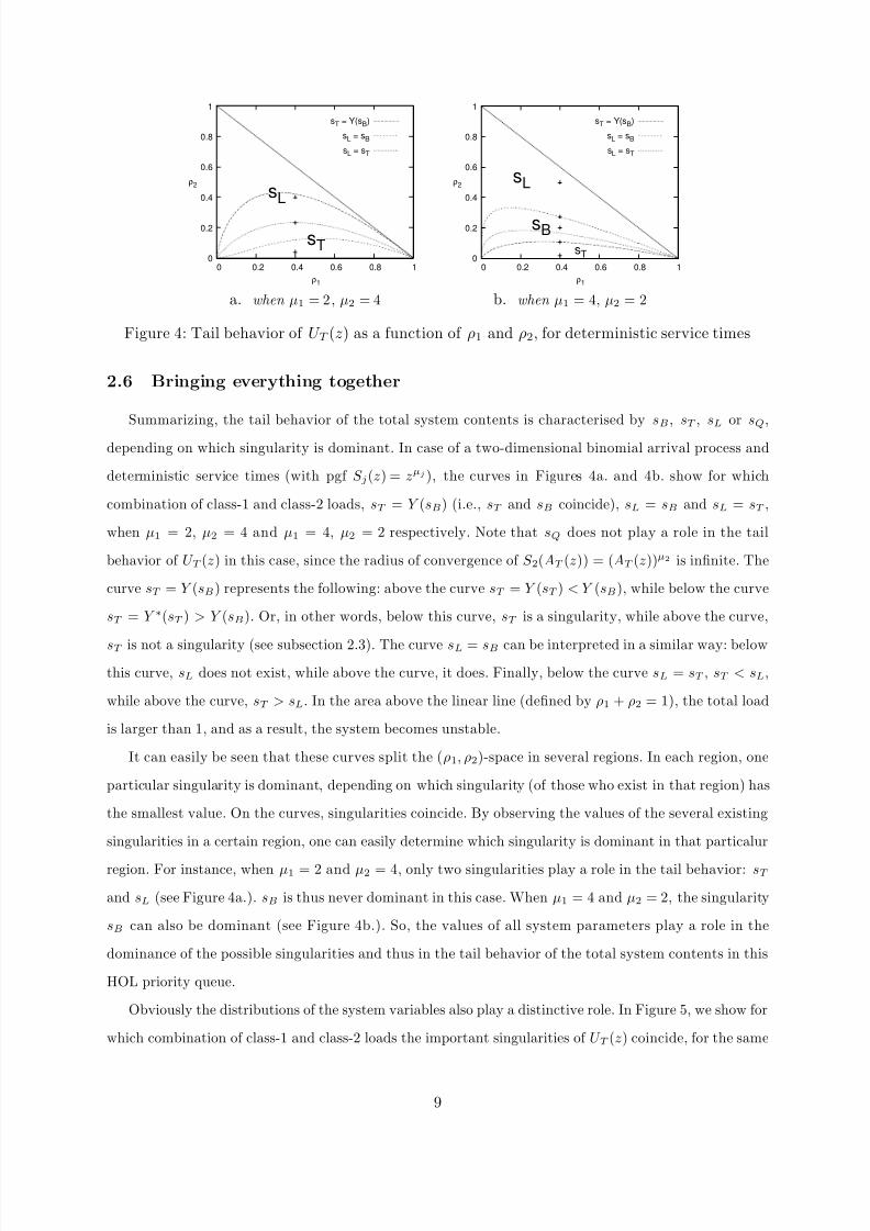
Figure 4: Tail behavior of U T (z) as a function of ρ1 and ρ2, for deterministic service times

2.6 Bringing everything together

Summarizing, the tail behavior of the total system contents is characterised by sB, sT , sL or sQ,

depending on which singularity is dominant. In case of a two-dimensional binomial arrival process and

deterministic service times (with pgf S j(z) = zµj), the curves in Figures 4a. and 4b. show for which

combination of class-1 and class-2 loads, sT = Y (sB) (i.e., sT and sB coincide), sL = sB and sL = sT ,

when µ1 = 2, µ2 = 4 and µ1 = 4, µ2 = 2 respectively. Note that sQ does not play a role in the tail

behavior of U T (z) in this case, since the radius of convergence of S 2(AT (z)) = (AT (z))µ2 is infinite. The

curve sT = Y (sB) represents the following: above the curve sT = Y (sT ) < Y (sB), while below the curve

sT = Y ∗(sT ) > Y (sB). Or, in other words, below this curve, sT is a singularity, while above the curve,

sT is not a singularity (see subsection 2.3). The curve sL = sB can be interpreted in a similar way: below

this curve, sL does not exist, while above the curve, it does. Finally, below the curve sL = sT , sT < sL,

while above the curve, sT > sL. In the area above the linear line (defined by ρ1 + ρ2 = 1), the total load

is larger than 1, and as a result, the system becomes unstable.

It can easily be seen that these curves split the (ρ1, ρ2)-space in several regions. In each region, one

particular singularity is dominant, depending on which singularity (of those who exist in that region) has

the smallest value. On the curves, singularities coincide. By observing the values of the several existing

singularities in a certain region, one can easily determine which singularity is dominant in that particalur

region. For instance, when µ1 = 2 and µ2 = 4, only two singularities play a role in the tail behavior: sT

and sL (see Figure 4a.). sB is thus never dominant in this case. When µ1 = 4 and µ2 = 2, the singularity

sB can also be dominant (see Figure 4b.). So, the values of all system parameters play a role in the

dominance of the possible singularities and thus in the tail behavior of the total system contents in this

HOL priority queue.

Obviously the distributions of the system variables also play a distinctive role. In Figure 5, we show for

which combination of class-1 and class-2 loads the important singularities of U T (z) coincide, for the same

9



0

0.2

0.4

0.6

0.8

1

0 0.2 0.4 0.6 0.8 1

ρ1

ρ2 sL

sTsQ

sQ = sTsL = sTsL = sQ

0

0.2

0.4

0.6

0.8

1

0 0.2 0.4 0.6 0.8 1

ρ1

ρ2 sL

sT

sB

sL = sB

sL = sT

sT = Y(sB)

a. when µ1 = 2, µ2 = 4 b. when µ1 = 4, µ2 = 2

Figure 5: Tail behavior of U T (z) as a function of ρ1 and ρ2, for geometric service times

two-dimensional binomial arrival process but for geometric service times with pgf’s S j(z) =z

z − µj(z − 1)( j = 1, 2), with µ1 = 2, µ2 = 4 (Figure 5a.) and µ1 = 4, µ2 = 2 (Figure 5b.). We observe that the (ρ1, ρ2)-

space again is split in several regions. sT , sL, or sQ determine the tail behavior of U T (z) when µ1 = 2,

µ2 = 4 (see Figure 5a.), while U T (z) is dominated by sT , sL, or sB when µ1 = 4, µ2 = 2 (see Figure

5b.). When the service times are geometrically distributed, the radius of convergence of S 2(AT (z)) may

thus determine the tail behavior of the total system contents.

2.7 The behavior of U T (z) in its dominant singularity

The type of the (co-)dominant singularity has a large impact on the tail behavior (see e.g. [8, 17]). In

this subsection, we use s∗ as a general notation for the dominant singularity of U T (z). According tothe previous subsection, three possible cases are established for s∗: s∗ = sB, s∗ = sB and sB is single-

dominant, or s∗ = sB but other singularities are co-dominant. In the remainder, we formulate a procedure

to approximate U T (z) in the neighbourhood of s∗, for each case. We refer to Appendix B for applications

of this procedure.

In the first case, the branch point sB is not dominant and a ’regular’ pole is the dominant singu-

larity. We replace each factor of U T (z) by its nth-order Taylor-series approximation in s∗, with n the

multiplicity of s∗ as zero of that factor. This leads to U T (z) ≈ K (∗)T

(s∗−

z)mfor z → s∗, with K

(∗)T a constant

and with m the multiplicity of the dominant singularity.

In the second case, in which the branch point sB is the only dominant singularity, we first substitute ex-

pression (3) of Y (z) in (1). Secondly, the obtained expression is rationalised, i.e., all roots are removed from

the denominator. We furthermore replace each factor of the denominator by the 0th-order Taylor-series

approximation in sB (since sB is not a zero of the denominator). We then get an expression for U T (z) of the

form U T (sB)−K (∗)T (sB − z)1/2 −K

(∗∗)T (sB − z) in the neighourhood of sB. Since the last term tends to

zero faster than the second term, we can omit the last term, yielding U T (z) ≈ U T (sB)−K (∗)T (sB − z)1/2

10



1e-07

1e-06

1e-05

0.0001

0.001

0.01

0.1

1

0 5 10 15 20 25 30 35 40

n

ρ1=0.4, ρ2=0.04 (A)ρ1=0.4, ρ2=0.23 (B)ρ1=0.4, ρ2=0.4 (A)

1e-07

1e-06

1e-05

0.0001

0.001

0.01

0.1

1

0 10 20 30 40 50 60 70 80

n

ρ1=0.4, ρ2=0.02 (A)ρ1=0.4, ρ2=0.10 (D)ρ1=0.4, ρ2=0.2 (C)ρ1=0.4, ρ2=0.27 (D)ρ1=0.4, ρ2=0.5 (A)

a. µ1 = 2, µ2 = 4 b. µ1 = 4, µ2 = 2

Figure 6: Tail probabilities of the total system contents for some (ρ1, ρ2)-combinations

for z → sB.

Finally, in the third case, the branch point sB is dominant together with other singularities. First,

we replace each factor of (1) in which Y (z) does not appear by its nth-order Taylor-series approximation

in sB. Secondly, we substitute Y (z) by its approximate expression (3). Finally, we separately look in the

numerator and the denominator for the term that tends to zero the slowest. This eventually leads to

U T (z) ≈ K (∗)T

(sB − z)m/2, with m an integer.

2.8 Obtaining expressions for the tail probabilities

In this subsection, we will focus on the special case of deterministic service times. Other distributions

of service times can be treated in a similar way. For each possible combination of dominant singularities

appearing in Figure 4, we can approximate U T (z) in the neighbourhood of its dominant singularity by

using the procedure in the previous subsection. We encounter 4 different tail behaviors for U T (z) in

this case, depending on which type of singularity dominates: a simple pole (behavior A), a pole with

multiplicity 2 (behavior B), a branch point (behavior C) or a simple pole coexisting with a branch point

(behavior D). Using Darboux’s theorem (see Appendix A), we finally find the tail probabilities for these

4 different cases:

uT (n) Prob[uT = n] ≈

K ∗T s−n−1∗

behavior A

K ∗T (n + 1)s−n−2∗ behavior B

K ∗T n−3/2s−n

∗

2

π/s∗behavior C

K ∗T n−1/2s−n

∗√πs∗

behavior D

, (6)

with s∗ a general notation for the dominant singularity and K (∗)T easily obtained according to the procedure

described in the previous subsection. Behavior A constitutes a typical geometric (exponential) behavior -

as encountered in many other queueing studies - while the others are non-geometric.

11



Figures 6a. and 6b. show the tail probabilities of the total system contents for the ( ρ1, ρ2)-combinations

indicated by the marks in Figures 4a. and 4b. respectively, when µ1 = 2 and µ2 = 4 and µ1 = 4 and

µ2 = 2. Note that the capital letter next to a (ρ1, ρ2)-combination in the legend of Figures 6a. and 6b.,

indicates the type of behavior (A, B, C or D) to which that particular combination belongs. Further, we

have compared our approximations with simulation results (marks in Figures 6a. and 6b.). The figures

show that the accuracy of the exponential (behavior A) asympotic approximations is excellent, while

the non-exponential approximations are not as accurate as the exponential ones. The minor accuracy of

the non-exponential approximations is attributed to the slower rates of convergence in the corresponding

expressions (see e.g. [8]).

3 The delay of a low-priority packet in a HOL-PJ queue

3.1 Preliminaries

As a second example of a priority queueing system quantity with a complex tail behavior, we consider

the delay of a low-priority packet in a single-server, two-class HOL-PJ (HOL priority with priority jumps)

queue. The waiting room is considered infinite and the arrival process is the same as in the first example,

i.e., a joint pgf A(z1, z2) for the numbers of arrivals of both classes, and marginal pgf’s AT (z) (= A(z, z)),

A1(z) (= A(z, 1)) and A2(z) (= A(1, z)) for the total number, the number of class-1 and the number

of class-2 arrivals respectively (with λj the arrival rate of class j, and λT = λ1 + λ2 the total arrival

rate). Note that in most figures in this section, we again use a two-dimensional binomial arrival process,

with joint pgf A(z1, z2) = (1 − λ1(1 − z1)/N − λ2(1 − z2)/N )N (where N = 16). The service times are

deterministically distributed, and equal to 1 slot. Furthermore, the system is influenced by a jumping

process: the class-2 packets, which are initially stored in the low-priority queue, jump at the end of each

slot with a probability β to the high-priority queue, in which arriving class-1 packets are queued. Packets

in the high-priority queue, which are thus of class 1 or class 2, have obviously a higher priority than the

packets in the low-priority queue. In other words, only when the high-priority queue is empty, packets of

the low-priority queue can be served. This priority queueing system has been analyzed in [18] and the pgf

of the class-2 packet delay is found to be

D2(z) =

(1− λT )z

β (AT (z)−A1(z))(V 0(z)−AT (V 0(z)))

+(1− β )(AT (V 0(z))−A1(V 0(z)))(1 −A1(z))(z −AT (z))

λ2(z −AT (z))(1− (1 − β )A1(z))(V 0(z)−AT (V 0(z))). (7)

The function V 0(z) is a solution of x− (1−β )zA1(x) = 0, |x| < 1 and |z| < 1, and is thus implicitly given

by (1− β )zA1(V 0(z)).

12



0

2

4

6

8

10

12

14

0 0.5 1 1.5 2 2.5 3

z dB

x

V0(z)

V0*(z)

Figure 7: Solutions of x− (1− β )zA1(x) = 0

As for U T (z) in the previous section, it is not a priori clear what the dominant singularity is of

D2(z). This is, in the first place, due to the occurrence of the function V 0(z), which is only implicitly

defined and which shows a similar behavior as Y (z) (see subsection 2.2).

3.2 Singularity dB

Specifically, in Figure 7, we see that the functional equation x−(1−β )zA1(x) = 0 has two positive real

solutions, namely V 0(z) and V ∗0 (z) - where V 0(z) is a strictly increasing and V ∗0 (z) a strictly decreasing

function - and that those two solutions coincide for z = dB. The figure shows further that V 0(z) and

V ∗0 (z) are no longer properly defined for values of z beyond dB (z > dB). Since V 0(z) remains finite and

V 0(z) →∞ in dB, we can easily determine the branch point dB:

V 0(dB) = (1− β )dBA1(V 0(dB))

V 0(dB) →∞⇒ V 0(dB)− (1− β )dBA1(V 0(dB)) = 0

(1− β )dBA

1(V 0(dB)) = 1. (8)

In the same way as Y (z), V 0(z) is then approximated by

V 0(z) ≈ V 0(dB)−K V (dB − z)1/2, (9)

where K V can be found by substituting z = dB in the latter expression, and by using the definition of

V 0(z):

K V =

2A1(V 0(dB))

dBA

1(V 0(dB)). (10)

3.3 Singularity dT

A second potential singularity dT of D2(z) on the real positive axis is given by the zero of z −AT (z)

larger than 1 (see Figure 8).

13



0

0.5

1

1.5

2

2.5

3

3.5

4

0 0.5 1 1.5 2 2.5 3 3.5 4

z dT

z

AT(z)

Figure 8: The functions z and AT (z) for z real and positive

0

2

4

6

8

10

0 0.5 1 1.5 2 2.5 3

zv1 v2

1

dT

V0(z)

AT(V0(z))

0

1

2

3

4

5

6

0 0.5 1 1.5 2 2.5 3

zv1

V0(z)

AT(V0(z))

a. dV exists b. dV does not exist

Figure 9: The singularity dV

3.4 Singularity v2

Thirdly, we look at the zeros of V 0(z) − AT (V 0(z)), which may be singularities of (7), since V 0(z) −AT (V 0(z)) is a factor of the denominator. We first rewrite V 0(z)− AT (V 0(z)) as the following system of

equations:

x−AT (x) = 0

x = V 0(z). (11)

The equation x − AT (x) = 0 has two positive real solutions, namely x = 1 and x = dT (see subsection

3.3). So V 0(z) − AT (V 0(z)) may have two real positive solutions v1 and v2, satisfying V 0(v1) = 1 and

V 0(v2) = dT respectively (see Figure 9a.). However, v1 is never a singularity of D2(z) since the numerator

of (7) is also zero for V 0(v1) = 1. Secondly, v2 does not always exist, since V 0(z) ceases to exist for z > dB,

and thus the second solution is not always ’reached’ before dB (see Figure 9a.). Whether the singularity

v2 exists or not, depends on the values of all system parameters: the arrival process and the jumping

probability β . When v2 exists, v2 =dT

(1− β )A1(dT ), which is easily checked by substituting V 0(z) by dT

in the definition of V 0(z). So, in summary, three cases can occur for the potential singularity v2: v2 exists

14



0

1

2

3

4

5

6

7

0 0.5 1 1.5 2 2.5 3

z

d1

x

d1=V0(d1)

V0(z)

V0*(z)

z

(1-β)zA1(z)

0

1

2

3

4

5

6

7

0 0.5 1 1.5 2 2.5 3 3.5 4

z

d1

x

d1=V0*(d1)

V0(z)

V0*(z)

z

(1-β)zA1(z)

a. d1 = V 0(d1) b. d1 = V ∗0 (d1)

Figure 10: The singularity d1

and v2 < dB, v2 exists and v2 = dB or v2 does not exist.

3.5 Singularity d1

A fourth potential singularity of D2(z) on the real positive axis (> 1) - denoted by d1 - is given by

the zero of 1 − (1 − β )A1(z). d1 is however not always a singularity, as we will show in the remainder

of this subsection. It is easily seen that (x, z) = (d1, d1) is a solution of x − (1 − β )zA1(x) = 0. This

equation, which has been discussed in subsection 3.2, has no solutions for z > dB, positive real. Hence,

d1 has to be smaller than dB . For z < dB , this equation has two positive real solutions (x, z), namely

(V 0(z), z) and (V ∗0 (z), z). Consequently, d1 = V 0(d1) or d1 = V ∗0 (d1) (see Figure 10). We can now verify

that when d1 = V 0(d1), d1 is also a zero of the numerator of D2(z) (see expression (7)), and thus not asingularity of D2(z). On the other hand, when d1 = V ∗0 (d1), d1 is not a zero of the numerator, and is

thus a singularity of D2(z). To conclude this subsection, we state the three possible cases for the potential

singularity d1: d1 = V 0(d1) < V 0(dB), d1 = V 0(dB) (in which case the branch point dB and d1 coincide)

and d1 = V ∗0 (d1) > V 0(dB). d1 is a singularity in the second and third case.

3.6 Determining the tail probabilities

First note that it can be proven that in this case the radii of convergence of the generating functions

appearing in (7) are never dominant. We can thus bring everything together: the singularities dB, dT , v2

or d1 - depending on which one is dominant - characterize the tail behavior of the class-2 delay. Their

mutual behavior, illustrated in Figures 11a. and 11b. for a two-dimensional binomial arrival process, and

for β = 0.4 and β = 0.75 respectively, can be determined in a similar way as in subsection 2.6: first

we calculate for which combinations of class-1 and class-2 loads singularities coincide, and then for each

region we determine which singularity is dominant.

Remark that in the area above the linear line in Figures 11a. and 11b. (defined by λ1+λ2 = 1), the total

15



0

0.2

0.4

0.6

0.8

1

0 0.2 0.4 0.6 0.8 1

λ1

λ2 dT

v2

dB d1

dT

d1 = V0(dB)

dT = dB

dT = v2

dT = d1

v2 = dB

0

0.2

0.4

0.6

0.8

1

0 0.2 0.4 0.6 0.8 1

λ1

λ2

d1

dT

dT = d1

v2 = dB

a. when β = 0.4 b. when β = 0.75

Figure 11: Tail behavior of D2(z) as a function of the arrival rates of both classes

1e-07

1e-06

1e-05

0.0001

0.001

0.01

0.1

1

0 5 10 15 20 25 30 35 40

n

λ1=0.2, λ2=0.25λ1=0.2, λ2=0.6λ1=0.6, λ2=0.01

1e-07

1e-06

1e-05

0.0001

0.001

0.01

0.1

1

0 5 10 15 20 25 30 35 40

n

λ1=0.2, λ2=0.31λ1=0.6, λ2=0.13λ1=0.51, λ2=0.19

a. behavior A b. behavior B

Figure 12: Tail probabilities of the class-2 delay for some (λ1, λ2)-combinations (1)

arrival rate is larger than 1, which results in an unstable system for these (λ1, λ2)-combinations. Figure

11a. shows that, when β = 0.4, all four singularities play a role in the tail behavior of D2(z). When

β = 0.75 on the other hand, only two singularities play a role: dT and d1 (see Figure 11b.). These figures

illustrate that again all system parameters - the arrival rates λ1 and λ2 and the jumping probability β -

influence the existence and dominance of the possible singularities, and thus have an impact on the tail

behavior of the class-2 delay in this HOL-PJ queue.

We can then formulate a similar procedure as in subsection 2.7 for approximating D2(z) in the neigh-

bourhood of its dominant singularity, necessary for the calculation of the tail probabilities. In this way,

we again encounter 4 distinct types of tail behavior.

Finally, by using Darboux’s theorem on the approximations of D2(z) in their dominant singularities,

the tail probabilities are calculated. Figures 12a., 12b., 13a. and 13b. show the tail probabilities of the

class-2 delay for the (λ1, λ2)-combinations indicated by the marks in Figure 11a.. Note that the tail

behavior of D2(z) depends on the type of the dominant singularity: a simple pole (behavior A), a pole of

multiplicity 2 (behavior B), a branch point (behavior C) or a simple pole coexisting with a branch point

(behavior D). The figures make clear that the approximate tail probabilities, compared to simulation

results, are again more than satisfactory.

16



1e-07

1e-06

1e-05

0.0001

0.001

0.01

0.1

1

0 5 10 15 20 25 30 35 40

n

λ1=0.2, λ2=0.01

1e-07

1e-06

1e-05

0.0001

0.001

0.01

0.1

1

0 5 10 15 20 25 30 35 40

n

λ1=0.2, λ2=0.21λ1=0.51, λ2=0.05

a. behavior C b. behavior D

Figure 13: Tail probabilities of the class-2 delay for some (λ1, λ2)-combinations (2)

4 Conclusions

In this paper, we have analyzed the tail behavior and derived approximate expressions for tail prob-

abilities of two particular variables in priority queueing systems, by means of the dominant singularity

approximation. We have shown that several singularities may play a role. Indeed, depending on the values

of the various system parameters, several singularities exist. Since each of them can be dominant, they all

determine the tail probabilities. We have furthermore shown that the number of singularities varies from

model to model. This makes studying the tail behavior much more complicated than in traditional queue-

ing models, and even more complicated than in “basic” priority queueing models. Furthermore, we have

proved that once the value of the dominant singularity is calculated, expressions of the tail probabilities

are easy to evaluate, which makes the dominant singularity approximation extremely suitable to study

these queueing systems. We have also compared our approximations with simulations, and the obtained

results are excellent. Altogether, this makes the dominant singularity method a very powerful technique

for deriving approximate expressions for tail probabilities in quite complicated queueing models.

Appendix A: Darboux’s theorem

Theorem 1.1 Suppose X (z) =∞

n=0 x(n)zn with positive real coefficients x(n) is analytic near 0 and

has only algebraic singularities αk on its circle of convergence|z|

= R, in other words, in a neighbourhood

of αk we have

X (z) ∼ (1− z

αk)−ωkGk(z), (12)

17



where ωk = 0,−1,−2, . . . and Gk(z) denotes a nonzero analytic function near αk. Let ω = maxkRe(ωk)

denote the maximum of the real parts of the ωk. Then we have

x(n) =

jGj(αj)

Γ(ωj)nωj−1α−nj + o(nω−1R−n), (13)

with the sum taken over all j with Re(ωj) = ω and Γ(ω) the Gamma-function of ω (with Γ(n) = (n− 1)!

for n discrete).

Appendix B: Examples of approximating U T (z) in the neighbour-

hood of its dominant singularity

In this appendix, we give 4 examples, in which the tail behavior of U T (z) is determined applying the

procedure described in subsection 2.7. In the first example, we consider the singularity sT to be the only

dominant singularity. Replacing factor z−S 1(AT (z)) by its first-order Taylor-series approximation (since

sT is a zero of this factor with multiplicity 1) and the remaining factors by their 0 th-order Taylor-series

approximation in expression (1), yields

U T (z) ≈

(1− ρT )(sT − 1)sT

(AT (sT )− 1)(sT − S 2(A(Y (sT ), sT )))

+(A(Y (sT ), sT )− 1)(S 2(AT (sT ))− S 1(AT (sT )))

(sT −

S 2(A(Y (sT ), sT )))(AT (sT )−

1)(S

1

(AT (sT ))A

T

(sT )−

1)(sT −

z),

or thus U T (z) ≈ K (∗)T

(sT − z)for z → sT (with K

(∗)T easily obtained from the latter expression).

In the second example, sT is co-dominant with sL. Following the same procedure as in the previous

example, we find

U T (z) ≈ (1− ρT )(sL − 1)sL(A(Y (sL), sL)− 1)(S 2(AT (sL))− sL)

(AT (sL)− 1)(S 1(AT (sL))A

T (sL)− 1)(sL − z)

×S 2(A(Y (sL), sL) A(1)(Y (sL), sL)Y (sL) + A(2)(Y (sL), sL)−

1(sL

−z)

,

for z → sL = sT . This leads to U T (z) ≈ K (∗)T

(sL − z)2in the neighbourhood of sL = sT .

In the third example, the branch point sB is the only dominant singularity of U T (z). Substituting

18



expression (3) in (1) first produces

U T (z) ≈

(1− ρT )(z − 1)

S 1(AT (z))(AT (z)− 1)

z − S 2(A(Y (sB), sB))

+K Y S 2(A(Y (sB), sB))A(1)(Y (sB), sB)(sB

−z)1/2

+z (S 2(AT (z))− S 1(AT (z)))

×

A(Y (sB), sB)−K Y A(1)(Y (sB), sB)(sB − z)1/2 − 1

(z − S 1(AT (z)))(AT (z)− 1)

(z − S 2(A(Y (sB), sB)))

+K Y S 2(A(Y (sB), sB))A(1)(Y (sB), sB)(sB − z)1/2

,

and after rationalising, we obtain

U T (z) ≈

(1− ρT )(z − 1)

S 1(AT (z))(AT (z)− 1)

z − S 2(A(Y (sB), sB))


+z (S 2(AT (z))− S 1(AT (z)))

×


×

z − S 2(A(Y (sB), sB))

−K Y S 2(A(Y (sB), sB))A(1)(Y (sB), sB)(sB − z)1/2

(z

−S 1(AT (z)))(AT (z)

−1)(z

−S 2(A(Y (sB), sB)))2

−K 2Y S 2(A(Y (sB), sB))2A(1)(Y (sB), sB)2(sB − z)

.

We furthermore replace each factor of the denominator by the 0th-order Taylor-series approximation in

sB, yielding

U T (z) ≈

(1− ρT )(z − 1)

S 1(AT (z))(AT (z)− 1)

z − S 2(A(Y (sB), sB))


+z (S 2(AT (z))− S 1(AT (z)))

×


×

z − S 2(A(Y (sB), sB))

−K Y S 2(A(Y (sB), sB))A(1)(Y (sB), sB)(sB − z)1/2

(sB − S 1(AT (sB)))(AT (sB)− 1)(sB − S 2(A(Y (sB), sB)))2 .

19



We can now put U T (sB) in front:

U T (z) ≈

(1− ρT )(sB − 1)

S 1(AT (sB))(AT (sB)− 1)(sB − S 2(A(Y (sB), sB)))

+sB(A(Y (sB), sB)−

1)(S 2(AT (sB))−

S 1(AT (sB)))

(sB − S 1(AT (sB)))(AT (sB)− 1)(sB − S 2(A(Y (sB), sB)))

−

(1− ρT )K Y (sB − 1)sB(S 2(AT (sB))− S 1(AT (sB)))A(1)(Y (sB), sB)

×

sB − S 2(A(Y (sB), sB)) + (A(Y (sB), sB)− 1)S 2(A(Y (sB), sB)) (sB − z)1/2

(sB − S 1(AT (sB)))(AT (sB)− 1)(sB − S 2(A(Y (sB), sB)))2

−

(1− ρT )K 2Y (sB − 1)S 2(A(Y (sB), sB))A(1)(Y (sB), sB)2

×

S 1(AT (sB))(AT (sB)− 1)S 2(A(Y (sB), sB))− sB(S 2(AT (sB))− S 1(AT (sB)))

(sB − z)

(sB

−S 1(AT (sB)))(AT (sB)

−1)(sB

−S 2(A(Y (sB), sB)))2

.

This finally leads to U T (z) ≈ U T (sB)−K (∗)T (sB − z)1/2 for z → sB, since the last term tends faster to

zero than the second term.

Finally, in the last example, the branch point sB is co-dominant with sL. We first replace the factors

in which Y (z) does not appear by their 0th-order Taylor-series approximation in sB, and then substitute

expression (3) in (1). This produces

U T (z) ≈

(1− ρT )(sB − 1)S 1(AT (sB))(AT (sB)− 1)z − S 2(A(Y (sB), sB))


+sB(S 2(AT (sB))− S 1(AT (sB)))

×


(sB − S 1(AT (sB)))(AT (sB)− 1)

(z − S 2(A(Y (sB), sB)))


.

20



Reorganising the latter expression yields

U T (z) ≈

(1− ρT )(sB − 1)sB(A(Y (sB), sB)− 1)(S 2(AT (sB))− S 1(AT (sB)))

(sB − S 1(AT (sB)))(AT (sB)− 1)(z − S 2(A(Y (sB), sB)))

+(sB − S 1(AT (sB)))(AT (sB)− 1)K Y S

2(A(Y (sB), sB))A(1)(Y (sB), sB)(sB − z)1/2

+

(1− ρT )(sB − 1)K Y A(1)(Y (sB), sB)(sB − z)1/2

×

S 1(AT (sB))(AT (sB)− 1)S 2(A(Y (sB), sB)) + sB(S 2(AT (sB))− S 1(AT (sB)))

(sB − S 1(AT (sB)))(AT (sB)− 1)(z − S 2(A(Y (sB), sB)))

+(sB − S 1(AT (sB)))(AT (sB)− 1)K Y S 2(A(Y (sB), sB))A(1)(Y (sB), sB)(sB − z)1/2

+

(1 − ρT )(sB − 1)S 1(AT (sB))(AT (sB)− 1)(z − S 2(A(Y (sB), sB)))

(sB

−S 1(AT (sB)))(AT (sB)

−1)(z

−S 2(A(Y (sB), sB)))

+(sB − S 1(AT (sB)))(AT (sB)− 1)K Y S 2(A(Y (sB), sB))A(1)(Y (sB), sB)(sB − z)1/2

.

Separately analysing the numerator and the denominator, and in both keeping the term that tends to

zero the slowest, finally approximates U T (z) byK

(∗)T

(sB − z)1/2in the neighbourhood of sB.

References

[1] J. Abate, G. Choudhury, D. Lucantoni, and W. Whitt. Asymptotic analysis of tail probabilities

based on the computation of moments. The Annals of Applied Probability , 5(4):983–1007, 1995.

[2] J. Abate, G. Choudhury, and W. Whitt. On the Laguerre method for numerically inverting Laplace

transforms. INFORMS Journal on Computing , 8:413–427, 1996.

[3] J. Abate, G. Choudhury, and W. Whitt. Numerical inversion of multidimensional Laplace transforms

by the Laguerre method. Performance Evaluation , 31(3-4):229–243, 1998.

[4] J. Abate and W. Whitt. The Fourier-series method for inverting transforms of probability distribu-

tions. Queueing Systems, 10:5–88, 1992.

[5] J. Abate and W. Whitt. Numerical inversion of probability generating functions. Operations Research

Letters, 12(4):245–251, 1992.

[6] J. Abate and W. Whitt. Solving probability transform functional equations for numerical inversion.

Operations Research Letters, 12:275–281, 1992.

[7] J. Abate and W. Whitt. Numerical inversion of Laplace transforms of probability distributions.

ORSA Journal on Computing , 7(1):36–43, 1995.

[8] J. Abate and W. Whitt. Asymptotics for M/G/1 low-priority waiting-time tail probabilities. Queueing

Systems, 25:173–233, 1997.

21



[9] J. C. P. Blanc. On the numerical inversion of busy-period related tranforms. Operations Research

Letters, 30:33–42, 2002.

[10] H. Bruneel, B. Steyaert, E. Desmet, and G.H. Petit. Analytic derivation of tail probabilities for queue

lengths and waiting times in ATM multiserver queues. European Journal of Operational Research ,

76:563–572, 1994.

[11] G. Choudhury and D. Lucantoni. Numerical computation of the moments of a probability distribution

from its transforms. Operations Research , 44(2):368–381, 1996.

[12] G. Choudhury and W. Whitt. Computing transient and steady-state distributions in polling models

by numerical transform inversion. Performance Evaluation , 25:267–292, 1994.

[13] G. Choudhury and W. Whitt. Computing distributions and moments in polling models by numerical

transform inversion. Performance Evaluation , 25(4):267–292, 1996.

[14] M. Drmota. Systems of functional equations. Random Structures & Algorithms, 10(1-2):103–124,

1997.

[15] A. Elwalid and D. Mitra. Analysis, approximations and admission control of a multi-service mul-

tiplexing system with priorities. In Proceedings of the Fourteenth Annual Joint Conference of the

IEEE Computer and Communication Societies, pages 463–472, 1995.

[16] G.A. Frolov and M.Y. Kitaev. A problem of numerical inversion of implicitly defined Laplace trans-

forms. Computers Mathematics with Applications, 36(5):35–44, 1998.

[17] K. Laevens and H. Bruneel. Discrete-time multiserver queues with priorities. Performance Evaluation ,

33(4):249–275, 1998.

[18] T. Maertens, J. Walraevens, and H. Bruneel. On priority queues with priority jumps. Performance

Evaluation . To be published.

[19] T. Sakurai. Numerical inversion for Laplace transforms of functions with discontinuities. Advances

in Applied Probability , 36(2):616–642, 2004.

[20] S. Shakkottai and R. Srikant. Many-sources delay asymptotics with applications to priority queues.

Queueing Systems, 39(2-3):183–200, 2001.

[21] R. L. Strawderman. Computing tail probabilities by numerical Fourier inversion: the absolutely

continuous case. Statistica Sinica , 14:175–201, 2004.

[22] V. Subramanian and R. Srikant. Tail probabilities of low-priority waiting times and queue lengths

in MAP/GI/1 queues. Queueing Systems, 34(1-4):215–236, 2000.

[23] A. Sughara, T. Takine, Y. Takahashi, and T. Hasegawa. Analysis of a non-preemptive priority queue

with SPP arrivals of high class. Performance Evaluation , 21:215–238, 1995.

22



[24] J. Walraevens. Discrete-time queueing models with priorities. PhD thesis, Ghent University, 2004.

[25] J. Walraevens, B. Steyaert, and H. Bruneel. Performance analysis of the system contents in a

discrete-time non-preemptive priority queue with general service times. Belgian Journal of Operations

Research, Statistics and Computer Science (JORBEL), 40(1-2), 2000.

[26] J. Walraevens, B. Steyaert, and H. Bruneel. Performance analysis of a single-server ATM queue with

a priority scheduling. Computers and Operations Research , 30(12):1807–1829, 2003.

23

Documents

Queueing Systems07