Embed Size (px)
Citation preview

Chapter 6
Fracture toughness of the tensile
and compressive failure modes in
laminated composites
6.1 Introduction
Fibre breaking can take place during longitudinal tension or compression and, for
carbon/epoxy systems, the energy consumed by these failure processes is much larger
than for failures involving any matrix or matrix-fibre bond failure. In compression,
fibre breaking usually occurs as a result of the kinking process. Experimental de-
termination of the fracture toughness associated with both these fibre failure modes
(tensile failure and compressive kinking) is important for material characterization
and for numerical modelling. Currently, there are no standards to determine these
properties.
Leach and Moore [158] used three-point bend specimens with a (0)40 layup to
measure the fracture toughness of the tensile fibre failure mode of a carbon/ PEEK
composite, and reported a mode I critical energy release rate of 26 kJ/m2. The
technique used to introduce a pre-crack in the specimen was not discussed by the
authors. Jose et al. [161] used Compact Tension (CT) specimens (see Fig. 6.1(a))
made of M55J/ M18 carbon/epoxy with layup (0, 90)15, to determine the fracture
131

CHAPTER 6. FRACTURE TOUGHNESS OF THE TENSILE AND
COMPRESSIVE FAILURE MODES IN LAMINATED COMPOSITES 132
toughness associated with tensile failure of the (0, 90)15 laminate. They created the
pre-crack in two steps: a notch was cut with a disc cutter and a razor blade was
then used to give a sharp starter, but the authors did not specify whether the blade
was tapped or used in a sawing motion. The mode I critical energy release rate
reported by Jose et al. for the laminate is 15.94 kJ/m2. This value corresponds to
the mode I critical energy release rate for fibre fracture in the 0 ◦ layers combined
with matrix crack propagation in the 90 ◦ layers. Assuming that those energies are
additive (which is to say, neglecting the interactions between the different layers
that are failing in different failure modes), and that the matrix tensile toughness
is similar in magnitude to the (interlaminar) mode I critical energy release rate
(≈ 0.2 kJ/m2), the fracture toughness for the fibre tensile failure mode of M55J/
M18 carbon/epoxy is about 31.7 kJ/m2.
Soutis et al. [171, 172] carried out a kink-band propagation test using a centre-
notched compression specimen. Different lengths for the notch were used but similar
values of fracture toughness were observed, which was interpreted as supporting
the concept of compressive fracture toughness. For a T800/924C laminate with
(0, 902, 0)3S layup, the fracture toughness for the laminate was reported [152] as
38.8 kJ/m2. Proceeding as before, the value measured corresponds to the mode
I critical energy release rate for kink-band propagation in the 0 ◦ layers, plus the
critical energy release rate for matrix cracking in the 90 ◦ layers. Assuming that those
energies are additive, and that the matrix failure in the 90 ◦ layers can be represented
by a single mode II matrix crack (with critical energy release rate ≈ 1 kJ/m2), the
fracture toughness for kink-band formation and for T800/924C is derived from Soutis
et al. [152] as about 76 kJ/m2.
Ratcliffe et al. [173] and Jackson and Ratcliffe [174] described the use of Com-
pact Compression (CC) specimens (CC specimens are similar to CT specimens,
but used in compression) to measure the compressive toughness of sandwich panels
with carbon-epoxy facings and honeycomb nomex core. The kink-band length was
measured using Shadow Moire Interferometry. The critical energy release rate for
kinking, derived from the tests using the area method, was reported as 36.1 kJ/m2
[173].

CHAPTER 6. FRACTURE TOUGHNESS OF THE TENSILE AND
COMPRESSIVE FAILURE MODES IN LAMINATED COMPOSITES 133
Table 6.1: Mechanical properties of T300/913 unidirectional laminae.
Modulus (GPa) Major Poisson’s ratio
Longitudinal Transverse Shear
131.7 8.8 4.6 0.32
In the work presented in this thesis, CT and CC tests were performed with the
aim of determining (i) the fracture toughness associated with tensile fibre failure
and (ii) the fracture toughness associated with kink-band failure for a carbon-epoxy
system.
6.2 Material system used
Carbon epoxy T300/913 unidirectional prepreg was used for the tests. The material
properties needed for the data reduction were obtained using standard tests and are
presented in Table 6.1 in the principal material axes.
6.3 Test method and data reduction
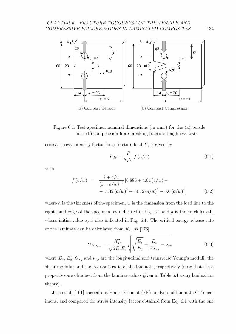
The geometry of the compact specimens used for the tension and compression tough-
ness tests are shown in Fig. 6.1(a) and (b) respectively. The notch of the CC
specimen, Fig. 6.1(b), has been widened at the left edge to avoid contact of the
notch faces during compression. (Jackson and Ratcliffe [174] found that the stress
intensity factor is not significantly affected by the morphology of the opening.) The
layup used is (90, 0)8S with the 0 ◦-direction the direction parallel to the loading, as
shown in Fig. 6.1.
The data reduction for CT or CC specimens made of an orthotropic material
requires particular attention. Other researchers have used the stress intensity fac-
tor approach [157, 159, 161], often citing the ASTM standard E399 [175] for the
determination of the fracture toughness in metals using CT tests [159, 161].
According to ASTM standard E399 [175], valid for an isotropic material, the
CHAPTER 6. FRACTURE TOUGHNESS OF THE TENSILE AND
COMPRESSIVE FAILURE MODES IN LAMINATED COMPOSITES 134
(a) C o m p ac t Te n s i o n (b ) C o m p ac t C o m p r e s s i o n
a � = 26
w = 51
14
28 60
φ8
h = 4
a � = 20
w = 51
14
28 60
φ8
h = 4
0º
≈4
≈20 ≈10
≈4 0º
≈10
Figure 6.1: Test specimen nominal dimensions (in mm ) for the (a) tensile
and (b) compression fibre-breaking fracture toughness tests
critical stress intensity factor for a fracture load P , is given by
KIc =P
h√wf (a/w) (6.1)
with
f (a/w) =2 + a/w
(1 − a/w)1.5 [0.886 + 4.64 (a/w)−
−13.32 (a/w)2 + 14.72 (a/w)3 − 5.6 (a/w)4] (6.2)
where h is the thickness of the specimen, w is the dimension from the load line to the
right hand edge of the specimen, as indicated in Fig. 6.1 and a is the crack length,
whose initial value ao is also indicated in Fig. 6.1. The critical energy release rate
of the laminate can be calculated from KIc as [176]
GIc|lam =K2Ic
√
2ExEy
√
√
√
√
√
Ex
Ey
+Ex
2Gxy
− νxy (6.3)
where Ex, Ey, Gxy and νxy are the longitudinal and transverse Young’s moduli, the
shear modulus and the Poisson’s ratio of the laminate, respectively (note that these
properties are obtained from the laminae values given in Table 6.1 using lamination
theory).
Jose et al. [161] carried out Finite Element (FE) analyses of laminate CT spec-
imens, and compared the stress intensity factor obtained from Eq. 6.1 with the one

CHAPTER 6. FRACTURE TOUGHNESS OF THE TENSILE AND
COMPRESSIVE FAILURE MODES IN LAMINATED COMPOSITES 135
obtained from FE. They concluded that the difference was small even though, when
expressed in terms of energy release rate, the difference ranged from 16% to 27%,
depending on the layup. The difference was attributed to the FE analysis being
linear, but Eq. 6.1 also assumes linear elasticity and so the difference is more likely
to be due to the isotropy assumption in Eq. 6.1.
Given the difference observed by Jose et al., an FE analysis was carried in Abaqus
[177] to obtain a more accurate equation for the fracture toughness. As a first step,
three different models of half a CT/CC specimen were created (taking advantage
of the symmetry), with different levels of mesh refinement. The three meshes have
uniform square 8-noded elements (S8R5), with side l = 1mm for the coarse (C)
mesh, l = 0.5mm for the intermediate (I) mesh and l = 0.2mm for the refined
(R) mesh. Mesh C is presented in Fig. 6.2, where it can be noted that the shape
of the notch is not modelled; as mentioned before, earlier work by Jackson and
Ratcliffe [174] showed that the stress intensity factor is not significantly affected by
the morphology of the opening. The material properties were obtained from Table
6.1 using lamination theory for a (90, 0)8S layup. All the models were assigned a
unit thickness (1mm ), and were subjected to a unit load (1N ). For a crack length
a = 26mm , each model was run to obtain the J-integral around the crack tip. Taking
the J-integral for mesh R as a reference, the J-integral for mesh I differs in 0.014%
and for mesh C in 0.026%. The application of the one-step Virtual Crack Closure
Technique (VCCT) for mesh R matches the J-integral for the same mesh within less
than 0.004%. Therefore, all three meshes (C, I and R) provide an accurate value of
the energy release rate. The difference between the energy release rate obtained by
the use of FE (J-integral, mesh R) and by the use of Eqs. 6.1 and 6.3 is 11.02%.
This considerable difference indicates that the KIc formula of Eq. 6.1 which is used
for isotropic materials is not accurate for orthotropic composites.
Several models with mesh I and different values of initial crack length were run.
The normalized energy release rate f (a), obtained from the J-integral (J), and
defined as
f (a) = J ·(
1mm
1N
)2
(6.4)

CHAPTER 6. FRACTURE TOUGHNESS OF THE TENSILE AND
COMPRESSIVE FAILURE MODES IN LAMINATED COMPOSITES 136
a
Figure 6.2: Coarse FE mesh of half a CT specimen
is presented in Table 6.2. The function f (a) can be approximated by the polynomial
f (a) = c3a3 + c2a
2 + c1a+ c0 (6.5)
where the coefficients ci are presented in Table 6.3 for a number of different crack
length ranges together with the associated interpolation error. Finally, the critical
energy release rate for each test can be obtained as
GIc|lam =
(
P
h
)2
f (a) . (6.6)
For the CT tests, Eq. 6.6 can be used to obtain GIc as a function of crack length
during propagation, provided that completely unstable propagation does not occur
immediately after initiation of crack growth. For fibre kinking however, Eq. 6.6
has limited meaning during propagation, because the contact stresses between the
‘faces’ of the kink band are not accounted for in the FE analysis, and neither is the
damage that might propagate from the kink band. An alternative method for data
reduction during propagation consists of the use of the area method in which the
energy consumed during crack growth (determined from the area under the load vs.
displacement curve) is divided by the area swept out by the crack front. However,
the application of this method requires stable crack growth, and, in the case of the
CC specimens, the calculated energy release rate will still include energy consumed
by other damage modes which are also developing as the kink band advances. This

CHAPTER 6. FRACTURE TOUGHNESS OF THE TENSILE AND
COMPRESSIVE FAILURE MODES IN LAMINATED COMPOSITES 137
Table 6.2: Normalised energy release rate f (a) (m2/kJ ) for different values
of crack length a (mm ), obtained from FE
a 19 20 21 22 23 24
f (a) 3.4003E-5 3.6753E-5 3.9839E-5 4.3320E-5 4.7272E-5 5.1788E-5
a 25 26 27 28 29 30
f (a) 5.6984E-5 6.3007E-5 7.0043E-5 7.8332E-5 8.8187E-5 1.0001E-4
a 31 32 33 34 35 36
f (a) 1.1436E-4 1.3196E-4 1.5381E-4 1.8132E-4 2.1646E-4 2.6207E-4
a 37 38 39 40 41 42
f (a) 3.2238E-4 4.0374E-4 5.1609E-4 6.7539E-4 9.0839E-4 1.2619E-3
a 43 44
f (a) 1.8229E-3 2.7642E-3
Table 6.3: Coefficients for the interpolation of f (a) ( m2/kJ ) for different
ranges of crack length a (mm ), and associated maximum error
c3 c2 c1 c0 error
19 ≤ a < 24 1.1250E-8 -5.088214E-7 9.7590E-6 -4.4897E-5 < 0.01%
24 ≤ a < 29 4.0880E-8 -2.6721E-6 6.2522E-5 -4.7474E-4 < 0.01%
29 ≤ a < 34 1.7282E-7 -1.4396E-5 4.1001E-4 -3.9105E-3 < 0.08%
34 ≤ a < 39 1.1264E-6 –1.1389E-4 3.8722E-3 -4.4084E-2 < 0.14%
39 ≤ a < 44 1.6611E-5 -1.9748E-3 7.8429E-2 -1.0399E0 < 0.80%

CHAPTER 6. FRACTURE TOUGHNESS OF THE TENSILE AND
COMPRESSIVE FAILURE MODES IN LAMINATED COMPOSITES 138
results in an artificial positive trend on the R-curves as verified by Jackson and
Ratcliffe [174].
Once the fracture toughness for the laminate is obtained, the fracture toughness
corresponding to fibre tensile failure or fibre kinking is obtained by subtracting the
term corresponding to matrix cracking in the 90 ◦ layers. This procedure neglects
the other damage modes such as delamination, as well as any interaction between
matrix cracking and the fibre-dominated failure modes, and assumes that a single
matrix crack parallel to the pre-crack occurs in the 90 ◦ layers. As before, matrix
cracking in the 90 ◦ layers is assumed to occur as a single crack in mode I for the CT
tests, and in mode II for the CC tests. These approximations seem reasonable, since
the fracture toughness of the fibre-dominated failure modes is much higher than
that of the matrix-dominated ones. For the laminate layup used for these tests, the
fracture toughness for the fibre-dominated failure modes is thus expressed as
GIc|fibre tensile = 2 GIc|lam tensile − GIc|matrix intra (6.7)
GIc|fibre kinking = 2 GIc|lam compr − GIIc|matrix intra (6.8)
where GIc|lam tensile and GIc|lam compr are the fracture toughness for the laminate,
as obtained from the tensile and compressive tests respectively, GIc|matrix intra and
GIIc|matrix intra are the mode I and mode II matrix-cracking intralaminar fracture
toughnesses, and GIc|fibre tensile and GIc|fibre kinking are the fracture toughnesses for
the fibre tensile and fibre-kinking failure modes. The mode I intralaminar fracture
toughness for through-the-thickness crack growth was found to be very similar to the
interlaminar toughness between 0 ◦ plies (Chapter 5), so that, for materials where
the matrix-cracking intralaminar fracture toughness is unknown, the interlaminar
fracture toughness is expected to be a good approximation of the intralaminar frac-
ture toughness. As noted above, in carbon/epoxy systems, the matrix failure mode
toughnesses are much lower than the fibre failure toughnesses and so the last term
in Eqs. 6.7 and 6.8 could be omitted without a significant loss in accuracy.

CHAPTER 6. FRACTURE TOUGHNESS OF THE TENSILE AND
COMPRESSIVE FAILURE MODES IN LAMINATED COMPOSITES 139
(a) (b)
Scale for moni-toring crack growth
Notch cut with disk saw
Notch cut with razor saw
Figure 6.3: Photograph of the specimens obtained for the (a) tensile and
(b) compression fibre fracture toughness tests
6.4 Manufacture
6.4.1 Manufacture of the test specimens
Panels with dimensions 300 × 150mm2 were manufactured by laying up 32 layers
of prepreg (each of 0.125mm nominal thickness), with a layup (90, 0)8S and cured
according to the prepreg manufacturer’s instructions. A wet saw was used to cut
the rectangular plates to form the specimens shown in Fig. 6.3. The 8mm diameter
holes were produced by drilling the specimen, with it held in between two sacrificial
pieces of similar composite.
For the tensile specimens, a 3-step procedure was followed to obtain the required
sharp crack tip. First, a 4mm wide notch was cut with a diamond-coated disk saw,
to a total approximate length of 30mm . Then, a 0.2mm thick razor saw was used
to obtain a thin and relatively sharp extension of the pre-crack, with a length of
approximately 10mm . Finally, a 0.1mm thick razor blade was used to sharpen the
crack tip further using a sawing action. Micrographs of the crack tip are presented
in Fig. 6.4. For the compression specimens, a notch as shown in Fig. 6.3(b) was
obtained with the disk saw.
A speckle pattern was created on one face of each specimen using white and
black ink sprays, in order to use a photogrammetry system. Two different types of

CHAPTER 6. FRACTURE TOUGHNESS OF THE TENSILE AND
COMPRESSIVE FAILURE MODES IN LAMINATED COMPOSITES 140
(a) (b )
(c ) (d )
0.5mm
62.5µµµµm
0.125mm
25µµµµm
1
2
1
3
2
3
1 Tw o d i f f e r e n t p l i e s e x p o s e d d u e t o p o l i s h i n g
R az o r s aw c u t
Ti p s h ar p e n e d b y r az o r b l ad e
Figure 6.4: Different magnifications of the pre-crack tip for the CT speci-
mens

CHAPTER 6. FRACTURE TOUGHNESS OF THE TENSILE AND
COMPRESSIVE FAILURE MODES IN LAMINATED COMPOSITES 141
pattern were tried: black spots on a white background and white spots on a black
background. The former was obtained by painting one side of the specimen in white
and then using the black-ink spray to obtain the speckle pattern. This process led
to a maximum contrast which is beneficial for the photogrammetry system software
monitoring each point of the specimen. However, in the tensile tests, the white ink
tended to peel at the crack tip during crack propagation. For these cases, the reverse
pattern was used (white spots an a black background), by simply using the white
spray to create the white spots on the black surface of the composite. The contrast
is in this case not as good as the previous one, but no peeling occurs at the crack
tip during propagation.
Finally, a 1mm increment scale was drawn onto each specimen to monitor the
crack length during the test, and the actual dimensions of each specimen were mea-
sured individually.
6.5 Experimental setup
The tests were carried out in an Instron machine, with a 10kN load cell. Two strong
light sources were used to illuminate the surface of the specimen.
A CCD camera was used to view a magnified image of the area of the specimen
containing the crack-growth scale an a TV. This magnified image was used together
with an event-marker connected to the data logger, to monitor the crack growth.
The photogrammetry system (Aramis) was positioned to examine the surface of
the specimen. This system allowed the strain field in the specimens to be recorded
during the tests and was used to check for damage not readily visible in the speci-
mens, and to help locate the tip of the crack/kink-band. The CT and CC specimens
were loaded at a displacement-rate of 0.5mm/min .

CHAPTER 6. FRACTURE TOUGHNESS OF THE TENSILE AND
COMPRESSIVE FAILURE MODES IN LAMINATED COMPOSITES 142
�����
� � � � ������ �����������������������
�! "�$#%��&"'(� )+* �,����-���.�-� /!0"1$2%354�6(7
89:;<=
8 9 : ;>@?�A�B�C 1�D�E-F.E-GIHJ3KF.F�7
LML ANB E-D ? F�E�G
( a ) ( b )
Figure 6.5: Typical load vs. displacement curves for a (a) CT and (b) CC
specimens
6.6 Results
6.6.1 Tensile tests
For the CT specimens tested, crack growth was not smooth nor continuous: instead,
several crack jumps of a few millimeters each time were observed, Fig. 6.5(a). The
TV monitor and event marker permitted the recording of the propagation load for
each value of crack length where the crack had stopped.
The first specimen tested had a black speckle pattern on a white background.
As the crack proceeded, the white ink peeled from the specimen on the vicinity of
the crack, and the photogrammetry system thus failed to map the strains on the
area of most interest, Fig. 6.6(a) and (b). For all other tensile specimens, a white
speckle on the natural black surface of the composite was used. This speckle had
a lower contrast, but still allowed the identification of the crack tip as no peeling
occurred, Fig. 6.6(c) and (d).
The R-curves obtained from the tensile tests are shown in Fig. 6.7. The average
fracture toughness obtained for initiation is 91.6 kJ/m2 with a standard deviation of
6.7%. Since the R-curves seem to converge after a ≈ 34 mm , a propagation value for
the fracture toughness can be defined. The average propagation fracture toughness

CHAPTER 6. FRACTURE TOUGHNESS OF THE TENSILE AND
COMPRESSIVE FAILURE MODES IN LAMINATED COMPOSITES 143
(a) (b )
No data from Photogrammetry system in this area
White paint has peeled off the specimen in this area
Pre-crack tip
Crack tip
(c ) (d )
Crack tip
Pre-crack tip
Crack tip
Pre-crack tip
Figure 6.6: (a) CT specimen painted white with black speckle pattern; the
paint peels off at the crack tip; (b) strain map corresponding to
(a) fails to give information close to the crack tip, due to peel-
ing of the paint; (c) CT specimen with white speckle pattern; no
peeling is observed at the crack tip; (d) strain map correspond-
ing to (c) allows the identification of the crack tip and does not
reveal any other form of damage in the specimen

CHAPTER 6. FRACTURE TOUGHNESS OF THE TENSILE AND
COMPRESSIVE FAILURE MODES IN LAMINATED COMPOSITES 144
0
5 0
1 00
1 5 0
2 00
2 5 0
2 4 2 9 3 4 3 9
a ( m m )
GIc ( k J / m2)
Figure 6.7: R-curve for the tensile fracture toughness tests; each symbol-
type corresponds to a different specimen
is 133.5 kJ/m2 with a standard deviation of 15.7%.
6.6.2 Compressive tests
For all but one of the CC specimens tested, the kink band grew smoothly during
the whole test (approximately 20mm of kink-band growth). In order to use the area
method to determine the critical energy release rate, the tests were carried during
kink band growth, and the unloading curve was recorded. Since no peeling of the
white ink occurred in compression, a black speckle on white background was used
for all tests.
The TV monitor, providing a magnified view of the region where the kink band
was growing, proved to be ineffective in locating the tip of the damaged area. In fact,
the tip of the kink band was barely recognizable on a still image, as shown in Figs.
6.8(a)-(c) of successive pictures taken by the photogrammetric system. Using the
photogrammetric system, the strain gradient proved useful to identify the existence
of the kink band, but the identification of the kink-band tip was not trivial, as
shown in Fig. 6.8(d). However, the identification of the tip of the damaged area was
possible using the photogrammetric system in a different way. A picture was taken

CHAPTER 6. FRACTURE TOUGHNESS OF THE TENSILE AND
COMPRESSIVE FAILURE MODES IN LAMINATED COMPOSITES 145
( d ) ( e ) ( f )
t = t � t = t � + 5 s t = t � + 1 0 s
( a ) ( b ) ( c )
Kink-band length
( b ) -( a )
Kink-band length
( c ) -( b )
Notch tip
Figure 6.8: (a) CC specimen during kink-band propagation at time t = to,
(b) at time t = to + 5s , (c) at time t = to + 10s ; (d) strain
map corresponding to (b); (e) difference between pictures (a)
and (b); (f) difference between pictures (b) and (c)
automatically by the system every 5 s and the event marker was used to identify
the load corresponding to that picture. The tip of the damaged area could then
be identified by switching repeatedly between two successive images taken by the
system. This dynamic viewing process showed the tip of the damaged area very
clearly, since the human eye has evolved to easily identify movement and thus the
difference between two pictures. As shown in Figs. 6.8(e) and (f), this difference
can also be obtained digitally, by subtracting two consecutive pictures taken by the
photogrammetric system.
The R-curves obtained from the compressive tests are shown in Fig. 6.9. The

CHAPTER 6. FRACTURE TOUGHNESS OF THE TENSILE AND
COMPRESSIVE FAILURE MODES IN LAMINATED COMPOSITES 146
0
1 00
2 00
300
4 00
5 00
1 8 2 3 2 8 33 38
a ( m m )
GIc ( k J / m2)
Values obtained by the ar ea m ethod f or 2 0 m m of k ink band g r ow th f r om initial c r ac k
Figure 6.9: R-curve for the compressive fracture toughness tests; each
symbol-type corresponds to a different specimen
average fracture toughness obtained for initiation is 79.9 kJ/m2 with a standard de-
viation of 7.7%. Using the area method, the average propagation fracture toughness
is 143.3 kJ/m2 with a standard deviation of 10.5%.
6.7 Discussion
6.7.1 Data reduction
The difference in the fracture toughness obtained using the data reduction from
ASTM standard E399 [175] for metals (isotropic material) and the FE approach
is found to be significant (11.0% for the material, layup and geometry considered
here), even though Ex and Ey were equal for the laminate layup used in these
tests. Therefore, the use of this standard for orthotropic composite materials is not
recommended.

CHAPTER 6. FRACTURE TOUGHNESS OF THE TENSILE AND
COMPRESSIVE FAILURE MODES IN LAMINATED COMPOSITES 147
6.7.2 Tensile tests
The specimen R-curves shown in Fig. 6.7 present the same trend even though the
pre-crack lengths vary. The GIc initiation values show good agreement and then
the curves all exhibit a positive trend over the next 4 − 8mm of crack growth.
Fig. 6.10(a) shows a Scanning Electron Microscope (SEM) image of the typical
fracture surface. It is not an entirely planar fracture surface, as it exhibits a limited
amount of fibre-pullout in the 0◦ plies. This pullout process could have created
a fibre-bridged zone in the wake of the advancing crack tip and the growth and
eventual stabilization of this bridged zone could account for the trend observed in
the R-curves.
The higher magnification image shown in Fig. 6.10(b) indicates that the 0◦
fibres immediately adjacent to the 90◦ ply interface are fractured without pullout.
The 0◦ fibres further away from the 90◦ ply interface have undergone pullout with
the fibre fracture occurring at some distance from the fracture surface in the 90◦
ply. The fracture features on the surface in the interface between the 90◦ and 0◦
plies shown in Fig. 6.10(b) indicate that the fracture occurred first in the 90◦ ply
and then propagated into the 0◦ ply.
Even though there is no visible damage away from the crack plane, as shown
by the C-scan in Fig. 6.11(a), the interaction of the 90◦ and 0◦ plies may signifi-
cantly affect the fracture process during propagation and so the propagation value
of fracture toughness is likely to be layup dependent.
It may well be that the lower initiation value of GIc is associated with an initial
planar fracture from the pre-crack plane without any significant fibre pullout—
and if this is the case, then the initiation value would be layup independent. The
mechanisms associated with the initiation and propagation fracture processes need
further investigation to fully establish their layup dependence.
6.7.3 Compressive tests
An increasing trend is exhibited by all the compressive-loading R-curves (Fig. 6.9)
and there is a good agreement in the initiation values. The positive trend in the

CHAPTER 6. FRACTURE TOUGHNESS OF THE TENSILE AND
COMPRESSIVE FAILURE MODES IN LAMINATED COMPOSITES 148
(b)
Fibre pullout
Limited or no fibre pullout
Shear cusps
(a )
Limited amount of fibre pullout in the 0° plies
Figure 6.10: (a) SEM micrograph of the CT specimen’s fracture surface; (b)
the magnitude of fibre pull out depends on the distance to the
90◦ layers

CHAPTER 6. FRACTURE TOUGHNESS OF THE TENSILE AND
COMPRESSIVE FAILURE MODES IN LAMINATED COMPOSITES 149
(a) (b)
Figure 6.11: C-scan of a (a) CT specimen and (b) CC specimen
R-curves, Fig. 6.9, can be explained by the contact forces in the kink-band faces.
However, the presence of these contact forces does not explain why the fracture
toughnesses obtained by the area method are higher than the initiation values de-
termined using Eqs. 6.6 and 6.8. In order to investigate whether the difference is due
to other damage modes (delamination, kink-band broadening, crushing), C-scans of
the failed specimens were performed, and several micrographs at different locations
along the kink-band path were obtained. The C-scan, Fig. 6.11(b), clearly shows
that kink-band propagation has been accompanied by delamination growth.
Several micrographs were taken from the tested specimens at specific cross-
sections, as shown in Fig. 6.12. Those taken from cross-section ‘A,’ i.e. next to
the tip of the kink band, are shown in Fig. 6.13, while those taken in cross-section
‘B,’ i.e. about 10mm behind the tip of the kink band, are shown in Fig. 6.14.
Fig. 6.13(a) shows a 0◦ ply in which the kink band has not yet fully developed.
Matrix cracking in the adjacent 90◦ plies and fracture in some of the 0◦ fibres can
be seen and these will ultimately develop into an out-of-plane kink band similar to
those shown in Fig. 6.13(b) and in magnified detail in Fig. 6.13(c). Fig. 6.13(d)
shows the matrix cracking and delamination which occurs in the 90◦ plies between
neighboring kink bands.
Turning to Fig. 6.14, it is clear that the scale of the fibre and matrix damage
is now more extensive than that close to the kink-band tip shown in Fig. 6.13. In
Fig. 6.14(a), the 0◦ plies clearly bent and in Fig. 6.14(b) the bending has caused

CHAPTER 6. FRACTURE TOUGHNESS OF THE TENSILE AND
COMPRESSIVE FAILURE MODES IN LAMINATED COMPOSITES 150
0º
B A
Figure 6.12: Cross-sections ‘A’ and ‘B’ for the micrographs shown in Figs.
6.13 (‘A’) and 6.14 (‘B’)
failure in the 0◦ fibres, i.e. the damage zone is broadening beyond that associated
with the initial kink-band formation. Figs. 6.14(c) and (d) show delaminations
which have been wedge opened by damaged material. These delaminations grow
significantly beyond the kink-band region, as detected by the C-scan image shown
in Fig. 6.11(b).
These findings, from analysis of the micrographs and C-scan images, imply that
the values of fracture toughness obtained by the area method do not describe ac-
curately the energy absorbed in kink-band formation, since other significant failure
modes have taken place. The initiation values seem to be the best measure of the
fracture toughness associated with kink-band formation.
6.8 Conclusions
This chapter has investigated an experimental procedure to obtain the fracture
toughness associated with the fibre-dominated failure modes, using CT and CC
tests. It has been shown that the data reduction process based on the stress in-
tensity factor for isotropic materials should not be used, and FE was found to be
a valid alternative. Initiation toughness values for both tensile fibre failure and for
kink-band formation were obtained. For the tensile mode, propagation toughness
values were also measured. For kink-band formation, propagation values cannot be

CHAPTER 6. FRACTURE TOUGHNESS OF THE TENSILE AND
COMPRESSIVE FAILURE MODES IN LAMINATED COMPOSITES 151
62.5µµµµm (a)
1
2
1
0.125mm(b )
3
3
1
25µµµµm (d )
4
3
1
0.125mm(c )
2
2
3
F i b r e b r e ak i n g 2
D e l am i n at i o n 4
M at r i x c r ac k i n g 1
K i n k b an d 3
Figure 6.13: Micrographs of the kink band in a CC specimen taken at sec-
tion ‘A’, see Fig. 6.12

CHAPTER 6. FRACTURE TOUGHNESS OF THE TENSILE AND
COMPRESSIVE FAILURE MODES IN LAMINATED COMPOSITES 152
(b)
5
3
0.25mm (a )
3
2
1
4
0.25mm
3
(d )
1
0.25mm (c )
6
6
7
0.25mm
K i n k ba n d br o a d e n i n g 2
B e n t f i br e s 4
O r i g i n a l k i n k ba n d 1
C r u s h e d m a t e r i a l 3
D e l a m i n a t i o n 6 B e n t f i br e s br e a k i n g 5
W e d g e e f f e c t 7
Figure 6.14: Micrographs of the kink band in a CC specimen taken at sec-
tion ‘B’, see Fig. 6.12

CHAPTER 6. FRACTURE TOUGHNESS OF THE TENSILE AND
COMPRESSIVE FAILURE MODES IN LAMINATED COMPOSITES 153
obtained directly from a stress intensity factor approach because the contact stresses
in the faces of the kink band cannot be easily accounted for; the area method also
failed to produce meaningful results due to kink band broadening and delamination.
The toughness measured for both the tensile and compressive modes may well be
layup dependent and further investigation is required.
6.9 Publications
The work presented in this chapter resulted in the following publications1:
1. S. T. Pinho, P. Robinson, L. Iannucci, Fracture toughness of the fibre break-
ing modes in laminated composites, Tech. rep., Department of Aeronautics,
Imperial College London (2005)
2. S. T. Pinho, L. Iannucci, P. Robinson. Modelling failure using physically-
based 3D models and a smeared formulation. 15th International Conference
on Composite Materials (ICCM-15). Durban, South Africa, 27th June - 01st
July 2005
1Some of these publications include work from other chapters of this thesis and therefore feature
again in the list of publications at the end of the corresponding chapters.

Chapter 7
Conclusions
7.1 Decohesion element
Three different constitutive laws were implemented within an interface element for-
mulation into LS-Dyna [1]. The formalism used is relatively simple and modular,
allowing other constitutive laws to be added easily. Initiation criteria, which define
the maximum traction in mixed-mode situations, as well as propagation criteria,
which define the energy absorbed in mixed-mode situations, can also be added tak-
ing advantage of the modularity of the implementation.
Under certain conditions (e.g. high loading rates, high maximum traction, low
energy release rate, coarse mesh refinement), it was observed that the discontinuities
existing in the bilinear constitutive law resulted in numerical instabilities. These
were not observed for the 3rd order polynomial or linear-polynomial laws. However,
all formulations were shown to model appropriately mode I, mode II and mixed
mode I and II quasi-static crack propagation problems at lower loading rates.
The decohesion element was shown to accurately model a range of static delam-
ination problems.
7.2 Failure criteria
Each failure mode in fibre-reinforced composites needs a separate investigation. Fail-
ure criteria based on physically-based failure models are good candidates to correctly
154

CHAPTER 7. CONCLUSIONS 155
account for how different stress components interact to promote each failure mode.
In this work, 3D compressive (matrix and fibre) failure models that account for
in-plane shear nonlinearity and in-situ effects are developed.
The criteria proposed, and the physically-based models developed, are shown
to accurately predict particular failure envelopes and trends. The fibre compression
failure model proposed emphasizes the need for accurate characterization of the shear
behaviour and can be readily used in a stochastic formulation, since manufacturing
defects can be easily accounted for within the model.
7.3 FE smeared failure model
The implementation of the failure models and criteria in an FE smeared failure model
demonstrates that the key physical aspects observed in the failure of laminated
composites can be reproduced in FE, provided that sound, physically-based failure
criteria are implemented, and that failure propagation is handled appropriately. The
failure-models implementation is 3D, and allows the user to incorporate any in-plane
shear curve directly. In addition, the pathological mesh dependency characteristic
of CDM models is avoided using a smeared formulation. Finally, all parameters used
in the model have clear physical meaning, and they can be obtained from simple
tests.
7.4 Combination of the ply damage model with
the decohesion element
Examples have shown that the ply damage model can, to a certain extent, predict
delamination, because it is able to predict failure in a plane parallel to the interface
between plies. This approach to model delamination is not ideal, because the frac-
ture surface is represented by a layer of elements. By using decohesion elements,
a better representation of the delamination can be achieved, at the expense of ad-
ditional complexity to the model as well as computational time. The decision on

CHAPTER 7. CONCLUSIONS 156
whether to use decohesion elements to model delamination depends on the relative
importance of delamination and the other failure modes for each specific problem.
7.5 Intralaminar fracture toughness tests
This work shows that it is possible to manufacture unidirectional laminated panels
including straight and sharp pre-cracks, without damage ahead of the crack tip and
without causing significant distortion to the layers. This can be achieved following
the process referred to as method E in Chapter 5.
FPB tests were shown to yield values for the mode I intralaminar fracture tough-
ness with low scatter, which are close to the mode I interlaminar fracture toughness.
The results obtained seem to indicate that there is a correlation between ply dis-
tortion and an increased measured fracture toughness. However, for the specimens
tested (all specimens had sharp crack tips and no damage ahead of the crack tip
was present), this correlation is not strong.
Using a plastic film to create a pre-crack does not yield a straight pre-crack,
but the fracture toughness values obtained were found to be consistent with those
obtained using the metal-blade approach to create the pre-crack.
7.6 Fracture toughness of the fibre breaking modes
This work has investigated an experimental procedure to obtain the fracture tough-
ness associated with the fibre-dominated failure modes, using CT and CC tests. It
has been shown that the data reduction process based on the stress intensity factor
for isotropic materials should not be used, and FE was found to be a valid alter-
native. Initiation toughness values for both tensile fibre failure and for kink-band
formation were obtained. For the tensile mode, propagation toughness values were
also measured. For kink-band formation, propagation values cannot be obtained
directly from a stress intensity factor approach because the contact stresses in the
faces of the kink band cannot be easily accounted for; the area method also failed
to produce meaningful results due to kink band broadening and delamination. The

CHAPTER 7. CONCLUSIONS 157
toughness measured for both the tensile and compressive modes may well be layup
dependent and further investigation is required.
7.7 Overall conclusions
The work reported here demonstrates that using physically-based failure criteria
and modelling individual failure modes, taking into account the associated fracture
toughness, are important for correctly modelling failure and crush of laminated com-
posite structures. Correctly modelling failure onset (using physically-based failure
criteria) and propagation (taking into account the fracture toughness correspondent
to each failure mode) is a significant step forward towards the accurate simulation
of complex structures under crush situations.

Chapter 8
Future work
8.1 Numerical
8.1.1 Further developments of failure criteria for laminated
composites
The 3D failure criteria developed in this thesis cover several failure modes, consider-
ing in-plane shear nonlinearity and in-situ effects. However, there are developments
that could be investigated if more extensive experimental data could be collected. In
particular, physical models for the effect of the in-plane transverse stress on the in-
plane shear nonlinearity could be developed. Also, the fibre-kinking model assumes
that failure takes place by matrix failure in the misalignment frame; even though
this assumption is reasonable for carbon-fibre reinforced composites, a broader model
should also consider the possibility of fibre micro-buckling, fibre-resin adhesion, and
fibre compression failure.
8.1.2 Further developments for the current FE failure model
In numerical simulations of crush situations, the debris composed of failed elements
causes numerical problems due to the significant distortions that can be obtained.
Furthermore, the modelling of a fracture plane within a failed element might not
be the best representation for debris that has separated from the main structure.
158

CHAPTER 8. FUTURE WORK 159
For these reasons, further developments into the post-failure behaviour might be
opportune.
8.1.3 Investigation of failure modes and damage models for
other fibre architectures
Woven textiles and other fabrics are increasingly being used in composites by the
industry. Failure modes for these materials are bound to be more complex than for
laminated composites with unidirectional plies. However, the knowledge obtained
for the laminated composites might prove useful in understanding failure for these
materials. Furthermore, once models and criteria for failure onset are developed for
these materials, the FE damage model developed in this thesis could be adapted for
other materials.
8.2 Experimental
8.2.1 Development and further validation of the fracture
toughness tests
The fracture toughness tests developed in this work are a first approach to obtain
the fracture toughness associated with different failure modes in composite materials
made of unidirectional plies. However, considerable research effort could be used in
investigating the effects of layup, specimen size and geometry, load rate, etc. in
order to fully validate these tests. Also the applicability of these test methods to
composites using woven or other forms of reinforcement could be investigated. The
test procedures developed for measuring the fracture toughness are already being
used with non-crimp fabrics manufactured by resin transfer moulding within the
Department of Aeronautics at Imperial College London.

CHAPTER 8. FUTURE WORK 160
8.2.2 Investigation into the test methodologies to obtain
failure data under combined load situations
One of the main difficulties associated with developing failure models and criteria is
the validation against experimental data. Considerable amounts of data are already
published for laminated composites, but there is still a need for a better definition
of failure envelopes under combined load situations. This investigation could lead
to the development of test methods for combined loading situations.
8.2.3 Investigation into in-situ effects
The work on in-situ effects reported here could be extended further. In this regard,
the experimental observations of fracture surfaces for specimens corresponding to
different in-situ conditions and the associated strength data could pave the way for
improved models for the in-situ effect.
8.2.4 Investigation of shear nonlinearity under complex loading-
unloading-reloading paths, and effect of in-plane trans-
verse stress on shear nonlinearity
The in-plane shear behaviour under complex loading-unloading-reloading paths was
found to be a point of difficulty in the present work, partly because of the lack of
experimental data. The effect of the in-plane transverse stress on the shear behaviour
is qualitatively known, but experimental data making quantitative characterization
for different material systems, as well as predictive physical models for this effect
are still in need of development.

Appendix A
Experimental stiffness and
strength characterisation
A.1 Introduction
The determination of the elastic properties and strength of unidirectional laminated
composites is important for design purposes, as well as numerical modelling. Fre-
quently, only the in-plane elastic properties are measured, leaving out the through-
the-thickness ones. This is due to a series of factors, such as:
• frequently, composites are analyzed using simplified models such as laminate the-
ory, and through-the-thickness properties are not always needed;
• the mechanical tests for measuring through-the-thickness properties are not so
widespread as the in-plane ones;
• economy reasons; and
• empirically, researchers have often found reasonable to estimate the through-the-
thickness properties from the in-plane ones, namely assuming that each uni-
directional laminae is transversely isotropic.
For these reasons, only in-plane properties are measured here. The material
tested is a carbon epoxy (T300/913), supplied by Hexcel; the fibre diameter is
about 7µm and the individual layer’s thickness is about 0.125mm .
161

APPENDIX A. EXPERIMENTAL STIFFNESS AND STRENGTH
CHARACTERISATION 162
Table A.1: In-plane mechanical properties, from the manufacturer
Longitudinal Transverse Shear
Tensile Compression Tensile Compression
Strength (MPa ) 2120 1450 68.1 225 -
Modulus (GPa ) 143 114 8.8 9.8 4.7
The in-plane properties for this material are provided by the manufacturer, Hex-
cel. However, elastic properties and strength are known to depend to a certain
extent on the manufacturing conditions (as well as testing). For this reason, com-
pression tests for the longitudinal direction (0◦ ) and transverse direction (90◦ ) are
planned, as well as in-plane shear tests and tensile tests at 0◦ . (Another motiva-
tion for carrying these tests is to achieve a deeper insight into the failure process,
specially for compression and shear.) Tensile tests in the matrix direction were not
carried essentially for material economy reasons. Table A.1 presents the properties,
as provided by Hexcel.
A.2 Data reduction
A.2.1 Compression
The compression tests were done according to the Imperial College London pro-
cedure for testing in compression [178]. The procedure and specimens are very
similar to the corresponding ASTM standard [179]. The main differences lie on the
geometry of the rig and the length of the specimens.
The strength values reported correspond to the higher stress registered during the
test. The Young’s modulus reported is the secant Young’s modulus taken at strain
levels of approximately 0.1% and 0.3% for the compression in the fibre direction,
and 0.2% and 0.4% for the compression in the transverse direction.
A.2.2 Tensile
The tensile tests were done according to the corresponding ASTM standard [180].

APPENDIX A. EXPERIMENTAL STIFFNESS AND STRENGTH
CHARACTERISATION 163
The strength values reported correspond to the higher stress registered during
the test. The Young’s modulus reported is the secant Young’s modulus taken at
strain levels of approximately 0.1% and 0.3% in the longitudinal direction. The
Poisson’s ratio is computed using the same values for the longitudinal strain.
A.2.3 Shear
The shear tests were done by testing a ±45◦ laminate in tension, according to the
corresponding ASTM standard [153].
The shear strain (γ) is computed from the longitudinal (εl) and transverse (εtr)
strains as
γ = εl − εtr. (A.1)
The shear stress (τ) could be computed from the load applied (P ) and initial cross-
sectional area (Ao) as suggested by the ASTM standard [153] as:
τ =P
2Ao
(A.2)
where P is the load and Ao is the initial cross-sectional area. For high shear strain
values (bigger than 5%), Eq. A.2 can be improved upon by considering the change
in the cross-sectional area and the rotation of the fibres, resulting in
τ =P
Asin
(π
4− γ
)
cos(π
4− γ
)
. (A.3)
In Eq. A.3, A is the cross-sectional area computed as A = t ×W (where t is the
thickness and W is the width of the specimen). The effect of width reduction was
considered by using an updated value for W , i.e.
W = Wo(1 − |εtr|)
where Wo is the initial width of the specimen. The strain values after failure of the
strain gauges were obtained by extrapolation using the strain rate observed for each
specimen before the strain gauges failed.
For the strength, both the higher stress registered during the test and the stress
at 5% shear strain are reported. The shear modulus reported is the secant shear
modulus taken at shear strain levels of approximately 0.2% and 0.6%.

APPENDIX A. EXPERIMENTAL STIFFNESS AND STRENGTH
CHARACTERISATION 164
(0°) ��� �������
� ���������
� �� ��� ��
���������! "�# $% "&'�(*)�+,.-/)�0(*)�+,�1 �
���������
� 2� ��� ��
P l a t e A
(0°) 3
�� ���������
�� 2� ���� 24
P l a t e B P l a t e A
±(4 5 °) 3 5
����������
�2 ����2 6
P l a t e C
Figure A.1: Plates manufactured for the in-plane tests
A.3 Manufacturing
Three plates, schematically represented in Fig. A.1, were manufactured by hand
lay-up. They were used for the manufacture of 0◦ and 90◦ compression specimens,
0◦ tensile specimens, and shear specimens, as detailed in Table A.2. The 0◦ and
90◦ compression specimens were labelled as ‘cl01’ to ‘cl22’ and ‘ctr01’ to ‘ctr08’,
respectively (the letter ‘c’ standing for compression, the letter ‘l’ for longitudinal
and the letters ‘tr’ for transverse); the 0◦ tensile specimens were labelled as ‘tl01’ to
‘tl06’ (the letter ‘t’ standing for tensile), and shear specimens were labelled as ‘s01’
to ‘s05’ (the letter ‘s’ standing for shear).
The curing cycle consisted of maintaining the temperature at 120◦ for 1 hour.
Individual specimens, with nominal dimensions shown in Table A.3 (see also Fig.
A.2) were then cut using a wet saw machine with diamond blade. Table A.3 also
shows the dimensions of the end tabs.
The effective width and thickness of each specimen were measured individually
for each specimen, and obtained as the average of three readings.

APPENDIX A. EXPERIMENTAL STIFFNESS AND STRENGTH
CHARACTERISATION 165
L b
t
h
W
Figure A.2: Representation of a specimen, with associated dimentions
Table A.2: Function and characteristics of the manufactured plates
Plate Test Dimensions number layup Thickness
(mm 2) of layers (mm )
A tensile 0◦ 300 × 150 8 (0◦ )8 1
B compression 0◦ and 90◦ 300 × 150 16 (0◦ )16 2
C shear 300 × 150 16 (±45◦ )8S 2
Table A.3: Nominal dimensions
Specimen L (mm ) W (mm ) t (mm ) b (mm ) h (mm )
cl 90 10 2 40 1.5
ctr 90 10 2 40 1.5
tl 250 15 1 56 1.5
s 250 25 2 56 1.5

APPENDIX A. EXPERIMENTAL STIFFNESS AND STRENGTH
CHARACTERISATION 166
Table A.4: Loading rate for each test type
Specimen type loading rate (mm/min )
cl 1.5
ctr 1.5
tl 2
s 2
(a) (b) (c) (d)
Figure A.3: (a) Experimental setup; (b) compression rig; (c) a ‘cl’ specimen;
(d) a ‘ctr’ specimen
A.4 Experimental
The tests were carried in a Zwick testing machine, in the Department of Aeronautics,
Imperial College London. The displacement rate specified in Table A.4 was applied.
Fig. A.3(a) shows the experimental setup, during a compression test.
A.4.1 Compression
For the compression tests, a small compressive preload was applied before tightening
the screws—Fig. A.3(b)—that fix the specimens in the rig (approximately 0.5kN
for the ‘cl’ specimens, and 0.2kN for the ‘ctr’ specimens). By doing this, it was
assured that the top and bottom surfaces of the specimens were in contact with
the rig. The torque applied to the screws is in accordance with Ref. [178]. The
specimens were then unloaded until there was no compression, before starting the
test. After the tests, each specimen was carefully examined to assess the failure

APPENDIX A. EXPERIMENTAL STIFFNESS AND STRENGTH
CHARACTERISATION 167
mode. For the ‘ctr’ specimens, the angle of the failure surface with the specimen’s
main direction was also measured. All specimens failed in a through-the-thickness
mode, at the interface between the tabs and the gauge (HAT and HAB designation
in the ASTM Compression Test Three-Part Failure Identification Code [179]), see
Fig. A.3(c) and (d). Specimen ‘ctr01’ was accidentally broken before the test.
A.4.2 Tensile
For the tensile tests, the specimens were carefully aligned to avoid bending. Failure
was explosive for all specimens (XUU designation in the ASTM Tensile Test Three-
Part Failure Identification Code [180]).
All specimens were strain gauged with a 3mm length 0◦ /90◦ rosette to measure
the strain in the longitudinal and transverse directions.
The load-strain data for specimen ‘tel05’ was accidentally lost immediately after
the test. Only the maximum load was recorded and as a result only the strength is
reported for that specimen.
A.4.3 Shear
The shear specimens were also carefully aligned with the loading direction. No
necking was observed before final failure took place, Fig. A.4. Failure always took
place in the gauge section (MGM designation in the ASTM Tensile Test Three-Part
Failure Identification Code [180]), Fig. A.5.
The loading of specimen ‘s01’ was stopped immediately after the strain gauges
failed (γ ≈ 4%), and the specimen was closely inspected after being taken out from
the Zwick machine. No damage was visible. After that, the specimen was loaded
again up to failure. Due to the residual strain from the first loading, no extrapolation
of the strains was possible for this specimen.

APPENDIX A. EXPERIMENTAL STIFFNESS AND STRENGTH
CHARACTERISATION 168
γ � ��� 2 . 1 1 4 . 4 2 2 . 9 2 6 . 1 2 7 . 0
Figure A.4: Evolution of damage during the test for specimen ‘s02’; the
shear strain at approximately the moment each picture was
taken is also shown; the last picture was taken about 3s before
complete failure
Figure A.5: Failed shear specimens

APPENDIX A. EXPERIMENTAL STIFFNESS AND STRENGTH
CHARACTERISATION 169
� � � � � � � �
� � � �
� � � �� � � � � � � �
� ��� �
� � � �� � � �� � � �
� ��� �
� � ��� � �
� � � �� � �
� ��� �
� � � �� � � �� � �
� � � �
� � � �� � �
�
� � �
��� �
� �
� � �
� � � �
� � � �
� ��� �
� � �
� �� � � � � � � � � � � � � � � � � � � � � � � � � � � � � � � � � � � � � � � � � � � � � � � � � � � � � � � � � �� � � �
Specimen
F a il u r e s t r es s ( M P a )
Figure A.6: Strength of each longitudinal compression specimen
A.5 Results
A.5.1 Longitudinal compression
The compressive strength of each longitudinal compression specimen is reported in
Fig. A.6. In the figure, specimens ‘ctr01’, ‘ctr11’, ‘ctr12’ and ‘ctr22’ are emphasized
because they were obtained from the edges of the plate. Specimens ‘ctr06’ to ‘ctr09’
are emphasized because they were the ones which were strain gauged. The percent
bending is presented in Fig. A.7 and the stress vs. strain relation in Fig. A.8. The
average strength is 1354.6MPa , with a coefficient of variation of 4.3%. The average
Young’s modulus is 116.1GPa , with a coefficient of variation of 2.4%.
A.5.2 Transverse compression
The compressive strength of each transverse compression specimen is reported in
Fig. A.9, the percent bending is presented in Fig. A.10 and the stress vs. strain
relation in Fig. A.11. The average strength is 198.6MPa , with a coefficient of
variation of 2.0%. The average Young’s modulus is 9.24GPa , with a coefficient of
variation of 1.2%.

APPENDIX A. EXPERIMENTAL STIFFNESS AND STRENGTH
CHARACTERISATION 170
0
10
2 0
3 0
40
5 0
0 0.2 0.4 0.6 0.8 1 1.2 1.4
A v e r a g e s t r a i n ( % )
By ( % )
c l 06 c l 07 c l 08
c l 09 c l 10
Figure A.7: Bending in the longitudinal compression specimens
0
5 00
1000
15 00
0 0.2 0.4 0.6 0.8 1 1.2 1.4
A v e r a g e s t r a i n ( % )
S t r e s s ( M P a )
c l 06 c l 07
c l 08 c l 09
c l 10
Figure A.8: Stress vs. strain relation for the longitudinal compression spec-
imens

APPENDIX A. EXPERIMENTAL STIFFNESS AND STRENGTH
CHARACTERISATION 171
201.0200.119 5 .919 7 .7205 .8
19 4 .819 5 .2
0
5 0
100
15 0
200
c t r 02 c t r 03 c t r 04 c t r 05 c t r 06 c t r 07 c t r 08
S p e c i m e n
M a x i m u m s t r e s s ( M P a )
Figure A.9: Strength of each transverse compression specimen
0
5
10
15
2 0
2 5
3 0
3 5
4 0
4 5
50
0 0.2 0.4 0.6 0.8 1 1.2 1.4 1.6 1.8
A v e r a g e s t r a i n ( % )
By ( % )
c t r 02 c t r 03 c t r 04
c t r 05 c t r 06
Figure A.10: Bending in the transverse compression specimens

APPENDIX A. EXPERIMENTAL STIFFNESS AND STRENGTH
CHARACTERISATION 172
0
2 0
4 0
6 0
80
100
12 0
14 0
0 0.2 0.4 0.6 0.8 1 1.2 1.4 1.6 1.8
A v e r a g e s t r a i n ( % )
S t r e s s ( M P a )
c t r 02 c t r 03
c t r 04 c t r 05
c t r 06
Figure A.11: Stress vs. strain relation for the transverse compression speci-
mens
A.5.3 Tensile
The tensile strength of each specimen is reported in Fig. A.12, the longitudi-
nal stress vs. strain relation is presented in Fig. A.13 and the transverse-strain
vs. longitudinal-strain relation are shown in Fig. A.14. The average strength is
2005.4MPa , with a coefficient of variation of 1.6%. The average longitudinal Young’s
modulus is 131.7GPa , with a coefficient of variation of 0.8%. The average major
Poisson’s ratio is 0.32, with a coefficient of variation of 2.6%.
A.5.4 Shear
The shear strength of each specimen is reported in Fig. A.15 and the shear stress
vs. strain relation up to strain gauges failure is presented in Fig. A.16. The strain
rate can be observed in Fig. A.17 up to strain gauge failure. The constant strain
rate in Fig. A.17 allows the extrapolation of the strain values beyond gauges failure,
allowing to draw the full stress vs. strain curves presented in Fig. A.18.
The average strength at 5% strain is 71.9MPa , with a coefficient of variation of
0.9%. The maximum stress during the test took place prior to failure. The average

APPENDIX A. EXPERIMENTAL STIFFNESS AND STRENGTH
CHARACTERISATION 173
20541 9 8 81 9 7 21 9 9 41 9 8 8203 7
0
500
1 000
1 500
2000
t e l 01 t e l 02 t e l 03 t e l 04 t e l 05 t e l 06S p e c i m e n
Fa
ilu
re s
tres
s (M
Pa
)
Figure A.12: Strength of each tensile specimen
0
5 00
1000
15 00
2 000
0 0.2 0.4 0.6 0.8 1 1.2 1.4 1.6
L o n g i t u d i n a l s t r a i n ( % )
S t r e s s ( M P a )
t e l 01 t e l 02 t e l 03t e l 04 t e l 06
Figure A.13: Stress vs. strain relation for the tensile specimens

APPENDIX A. EXPERIMENTAL STIFFNESS AND STRENGTH
CHARACTERISATION 174
0
0. 2
0. 4
0 0. 5 1 1. 5L o n g i t u d i n a l s t r a i n ( % )
T r a n s v e r s e s t r a i n ( % )
t e l 01t e l 02t e l 03t e l 04t e l 06
Figure A.14: Transverse vs. longitudinal strain for the tensile specimens
Table A.5: Summary of the in-plane mechanical properties
Longitudinal Transverse Shear
Tensile Compression Compression 5% Max.
Strength (MPa )
(coef. of var.)
2005.4
1.6%
1354.6
4.3%
198.6
2.0%
71.9
0.9%
148.0
2.8%
Modulus (GPa )
(coef. of var.)
131.7
0.8%
116.1
2.4%
9.24
1.2%
4.6
2.8%
maximum stress is 148.0MPa , with a coefficient of variation of 2.4%. The average
shear modulus is 4.6GPa , with a coefficient of variation of 2.8%.
A.5.5 Summary
The main quantitative data resulting from these tests is presented in Table A.5. For
the in-plane major Poisson’s ratio, not shown in the table, the average is 0.32, and
the coefficient of variation is 2.6%.

APPENDIX A. EXPERIMENTAL STIFFNESS AND STRENGTH
CHARACTERISATION 175
150 150 14 914 3
7 2 7 2 7 3 7 2 7 1
0
4 0
8 0
12 0
16 0
s01 s02 s03 s04 s05S p ec imen
S h ear stren g th ( MP a)
S tress at 5%sh ear strain
Maximum stressd urin g test
Figure A.15: Shear strength as the stress at 5% shear strain and as the
maximum stress during the test
0
20
40
6 0
8 0
0 0. 5 1 1. 5 2 2. 5 3 3. 5 4
S h e a r s t r a i n ( % )
S h e a r s t r e s s ( M P a )
s 01 s 02
s 03 s 04
s 05
P o i n t w h e r e t h e s t r a i n g a u g e s
b r o k e
Figure A.16: Shear stress vs. strain relation, before failure of the strain
gauges

APPENDIX A. EXPERIMENTAL STIFFNESS AND STRENGTH
CHARACTERISATION 176
0
1
2
3
4
1 t i m e
S h e a r s t r a i n ( % )
s 02 s 03
s 04 s 05
Figure A.17: Shear strain rate before failure of the strain gauges
0
4 0
8 0
1 2 0
1 6 0
0 5 1 0 1 5 2 0 2 5 30
S h e a r s t r a i n ( % )
S h e a r s t r e s s ( M P a )
s 02 s 03
s 04 s 05
Figure A.18: Shear stress vs. strain curve obtained with extrapolated strain
values (after the failure of the strain gauges)

APPENDIX A. EXPERIMENTAL STIFFNESS AND STRENGTH
CHARACTERISATION 177
Table A.6: Difference between the obtained data and the one provided by
the manufacturer (%)
Longitudinal Transverse Shear
Tensile Compression Compression
Strength -5.7 -7.0 -13.3 -
Modulus -8.5 1.8 -6.1 -2.2
A.6 Discussion
A.6.1 Compression
All compression specimens failed in an acceptable failure mode. The average value
and the scatter in the results are acceptable. No effect on the strength of the position
of the specimen in the plate is observed. Nonlinear behaviour is observable for both
longitudinal and transverse loading. For the transverse specimens, some oscillations
are visible in the strain vs. stress curves, that are not completely understood, but
are probably related to the low stresses involved in the tests and the rig itself.
Improvements in the compressions tests could include trying different transition
geometries for the tabbed/ non-tabbed regions, in order to avoid failure in that
interface.
When comparing the obtained data (Table A.5) to the one provided by the man-
ufacturer (Table A.1), it can be realized that the obtained values for strength and
modulus are almost consistently below the ones provided by the manufacturer. The
difference for each situation are compiled in Table A.6. The difference is probably
related to the manufacturing, and eventually also the testing.
A.6.2 Tensile
All tensile specimens failed in an acceptable failure mode. The average value and
the scatter in the results are also acceptable. Again, no effect of the position of the
specimen in the plate on the strength is observable. The stress vs. strain relation is
reasonably linear up to failure.

APPENDIX A. EXPERIMENTAL STIFFNESS AND STRENGTH
CHARACTERISATION 178
A.6.3 Shear
All shear specimens failed in an acceptable failure mode. The average value and
the scatter in the results are also acceptable. The stress vs. strain curves up to
final failure were extrapolated. The linearity of the stress vs. strain curves and the
absence of necking before failure yields confidence to the extrapolation.
While these tests provide the (initial) in-plane shear modulus with accuracy, the
interpretation of the full nonlinear curve and the strength requires more caution. On
one hand, the 5% strength is useful for design purposes only, as it does not represent
material failure. On the other hand, the nonlinearity observed in the experiments
results from damage propagation in the composite; after a critical accumulation
of damage, failure of the specimen occurs. However, the propagation of shear-
driven damage in a ply depends on the thickness of the ply and the presence (and
stiffness) of neighboring plies (in-situ effect), as well as on the presence of stress
components other than in-plane shear τab. In the case of the ±45◦ test [153], each
individual ply is neighbored by plies at an angle of 90◦ (relatively to it) and an
in-plane transverse tensile stress σb is present together with the shear stress. As
a result, the nonlinear shear strain vs. shear stress curves obtained should not be
regarded as universal. Other shear test methods such as the Iosipescu [181], the
two-rail shear test [182] or the more recent V-notched rail shear method [183] (all
of them ASTM standards) should be carried to compare the nonlinear curve for
different situations. For the future, micro-mechanical models are good candidates
to predict the nonlinear behaviour and strength under simultaneously generic in-situ
and applied stress conditions, as well as loading-unloading-reloading situations. In
the absence of further data and such a model, the results obtained for the ±45◦ test
[153] are considered to represent the shear behaviour of the material system studied
(carbon epoxy T300/913).

Appendix B
Experimental interlaminar
toughness characterisation
B.1 Introduction
Delamination occurs when cracks grow between the layers of a (laminated) composite
material. Those cracks can grow in opening or shear modes, and severely weaken the
material. As a result, the characterization of laminated composite materials, on what
concerns their interlaminar fracture toughness, is of great importance. Moreover,
analytical and numerical tools used to model composite materials need interlaminar
fracture toughness values as input properties.
The material tested is a carbon epoxy (T300/913), supplied by Hexcel. The fibre
diameter is about 7µm and the individual layer thickness is about 0.125mm .
Several mechanical tests have been proposed to characterize the interlaminar
fracture toughness in mode I, II and mixed mode I and II.
For mode I, the test most commonly used is the Double-Cantilever Beam (DCB),
although others exist, such as the Wedge-Insert-Fracture (WIF), Double-Edge-Notched
(DEN), Vickers Indentation Crack (VIC), Single-Edge Notched (SEN) and Surface
Cracked (SC), all shown in Fig. B.1.
Mode II delamination is typically characterized using End-Loaded Split (ELS),
End-Notched Flexure (ENF) or Four-Point Bend (4ENF) specimens, as shown in
179

APPENDIX B. EXPERIMENTAL INTERLAMINAR TOUGHNESS
CHARACTERISATION 180
Figure B.1: Mode I test specimens, from Ref. [184]
Fig. B.2. From these, the 4ENF has the advantage of applying a constant moment,
but is relatively new and is still being investigated.
Experimental tests involving mixed-mode I and II include the Cracked-Lap Shear
(CLS), Double-End-Notched Flexure (DENF), Mixed-Mode Bending (MMB), Mixed-
Mode Flexure (MMF) or Single Cantilever Beam (SCB) tests, see Fig. B.3.
For mode I testing, the DCB is used in this work, for it is the most widely
used; the corresponding ASTM standard [30] is followed. The 4ENF test has been
recently proposed, and has the advantage of generating a constant moment to the
specimen in the region of the crack tip. For this reason, it is used in this work. The
data reduction follows Refs. [31, 32]. For I and II mixed-mode loading, the MMB
test has the advantage of allowing very easily to test different mode ratios, as this
does not require any change in the specimen geometry, but rather in the rig; the
corresponding ASTM standard [33] is followed for the data reduction.

APPENDIX B. EXPERIMENTAL INTERLAMINAR TOUGHNESS
CHARACTERISATION 181
Figure B.2: Mode II test specimens, from Ref. [184]
Figure B.3: Mixed mode I and II test specimens, from Ref. [184]

APPENDIX B. EXPERIMENTAL INTERLAMINAR TOUGHNESS
CHARACTERISATION 182
� �2�
������
2 �
� 2 �
����� �
2 �
� � �
�����
�
(a ) (b )
(c)
Figure B.4: (a) DCB, (b) 4ENF and (c) MMB specimens
B.2 Data reduction
B.2.1 Mode I
Following the ASTM standard for the DCB test [30], the mode I interlaminar frac-
ture toughness is calculated according to the modified beam theory,
GIc =3Pδ
2b (a+ |∆|) , (B.1)
where GIc is the fracture toughness, P is the load, δ is the opening displacement,
b is the specimen width, a is the crack length and ∆ is a correction term applied
to the crack length. It is determined from the experimental data after generating a
least square plot of the cubic root of compliance, C1/3, as a function of delamination
length, a. The correction term ∆ is the value that should be added to the crack
length to make the plot go through the origin. The compliance, C, is defined as
δ/P . This approach allows the bending modulus, Ef , to be determined as
Ef =64 (a+ |∆|)3 P
δbh3(B.2)
where h is the (total) specimen thickness, as shown in Fig. B.4(a).
Following the standard [30], large displacement and end block corrections were

APPENDIX B. EXPERIMENTAL INTERLAMINAR TOUGHNESS
CHARACTERISATION 183
applied to the previous expressions, but the effects of those corrections are very
small.
B.2.2 Mode II
The specimen design, experimental procedure and data reduction scheme proposed
by Martin and Davidson [31, 32] for the 4ENF test is used here. The half length
L in Fig. B.4(b) was chosen as 120mm , while the distance between the two load
points, d, is 80mm .
The results of the 4ENF test are calculated by considering the linear relationship
between compliance, C, and delamination length, a,
C = ma+ C0 (B.3)
and generating a least squares fit of the experimental data to determine m and C0.
The fracture toughness, GIIc, is then computed as
GIIc =mP 2
2b. (B.4)
The bending modulus can also be extracted from the test, using the relation [184]
Ef =9 (L− d/2)
8bh3m(B.5)
where h is half the thickness of the specimen (Fig. B.4), b is the width and Ef is
the bending modulus.
B.2.3 Mixed mode
Following the ASTM standard for the MMB test [33], the measurement of the
compliance of the loading system, Csys is required. This is done by using a stiff
rectangular-section calibration specimen instead of the MMB specimen. The com-
pliance of the calibration specimen is
Ccal =2L (c+ L)
Ecalbcalt3cal(B.6)

APPENDIX B. EXPERIMENTAL INTERLAMINAR TOUGHNESS
CHARACTERISATION 184
where Ecal, bcal and tcal are the modulus, width and thickness of the calibration spec-
imen. Being mcal the slope of the load vs. displacement curve, which is determined
experimentally, the compliance of the system is expressed as
Csys =1
mcal
− Ccal. (B.7)
This compliance is dependent on the lever length, c, and should therefore be deter-
mined for each value of c. The bending modulus, Ef , is obtained from
Ef =8 (ao + χh)3 (3c− L)2 +
[
6 (ao + 0.43χh)3 + 4L3]
(c+ L)2
16L2bh3 (1/m+ Csys)(B.8)
where ao is the initial crack length, m is the slope of the load vs. displacement curve,
h is the half thickness, L is the half length (Fig. B.4(c)) and
χ =
√
√
√
√
Ea
11Gac
[
3 − 2
(
Γ
1 + Γ
)2]
(B.9)
with
Γ = 1.18
√EaEb
Gca
. (B.10)
In the previous equations, Ea, Eb and Gca are the Young’s modulus in the longitudi-
nal and transverse directions and the shear modulus in the (a, c) plane, respectively.
The mode I component of the fracture toughness is
GI =4P 2 (3c− L)2
64bL2EfI(a+ χh)2 (B.11)
while the mode II component is
GII =3P 2 (c+ L)2
64bL2EfI(a+ 0.42χh)2 (B.12)
being I the moment of inertia of one arm of the specimen:
I =bh3
12. (B.13)
B.3 Manufacturing
A plate, schematically represented in Fig. B.5, was manufactured by hand lay-up.
The plate is 430 × 300mm 2 and consists of 24 unidirectional layers oriented at 0◦ ,

APPENDIX B. EXPERIMENTAL INTERLAMINAR TOUGHNESS
CHARACTERISATION 185
300
4 30
1 00 D e l a m .
2 4 p l i e s x 0°
D C B 4 E N F M M B
Figure B.5: Plate for DCB, 4ENF and MMB test specimens (dimensions in
mm)
being the nominal thickness 3mm . The layup was done in two halves of 12 layers. A
non-stick fluoroethylene polymer film, with a thickness of 12.5µm was then carefully
positioned on one half, before placing the other half on top to complete the assembly.
The curing cycle consisted of maintaining the temperature at 120◦ for 1 hour.
Individual specimens, with nominal dimensions shown in Table B.1 were then cut
using a wet saw. Five DCB specimens were manufactured, labelled as DCB01 to
DCB05. They were numbered in order from the left edge of the plate (Fig. B.5),
thus DCB01 being the one closer to the edge. The same procedure was repeated
for obtaining five 4ENF specimens, labelled as 4ENF01 to 4ENF05, and six MMB
specimens, labelled as MMB01 to MMB06 (the numbers always increasing from left
to right in Fig. B.5).
In order to enhance the visibility of the crack tip during the tests, one side of
each specimen was coated with a white paint. A vernier height gauge was then
used to mark a length scale on the painted side of the specimens. This scale was
used for measuring the crack length during the test. Finally, for the DCB and
MMB specimens, aluminum end tabs were glued using an epoxy glue (araldite).
The individual width and thickness of each specimen was measured experimentally
by averaging three individual measurements.

APPENDIX B. EXPERIMENTAL INTERLAMINAR TOUGHNESS
CHARACTERISATION 186
Table B.1: Nominal dimensions
Specimen Width (mm ) Initial crack (mm ) Length (mm )
DCB 20 53 150
4ENF 20 35 140
MMB 20 29 140
Table B.2: Cross head displacement rate for each test type
Specimen type displ. rate (mm/min )
DCB 0.5
4ENF 0.2
MMB 0.5
B.4 Experimental procedure
The tests were carried in a Instron testing machine, in the Department of Aero-
nautics, Imperial College London. The Instron machine outputs the load and dis-
placement as a voltage, to a data acquisition system connected to a computer. A
calibration of the factors needed to convert the voltage back into load and displace-
ment in the computer was carried for each set of tests (DCB, 4ENF and MMB).
For each specimen, the appropriate test rig was used. The Instron machine was
‘zeroed’ before each test and the cross head displacement rate specified in Table
B.2, was applied. The crack tip was monitored using a CCD camera, that displayed
an enlarged image in a TV screen. An event marker was used to send a signal to
the computer as the crack tip passed through each mark on the specimen. Fig. B.6
shows the experimental setup during a DCB test.
B.5 Results
B.5.1 DCB
Specimens DCB01 and DCB02 were not pre-cracked, and there was as a result
a crack jump of about 10mm at the onset of delamination. For this reason, the

APPENDIX B. EXPERIMENTAL INTERLAMINAR TOUGHNESS
CHARACTERISATION 187
Figure B.6: Experimental setup for the DCB test
remaining DCB specimens were pre-cracked in mode I. The load vs. displacement
curves for specimens DCB01 and DCB04 are shown in Fig. B.7. Fig. B.8 shows
the least squares fit used to obtain ∆ for specimen DCB05, and Fig. B.9 shows the
different values of ∆ for each DCB specimen. The cloud that results from plotting
all the R-curves (i.e. the curves that show the variation of Gc with crack length) is
shown in Fig. B.10, as well as the average value and coefficient of variation.
B.5.2 4ENF
All the 4ENF specimens were pre-cracked in mode II. The load vs. displacement
curve for specimen 4ENF04 is presented in Fig. B.11. The least squares fit used to
determine the slope of the load vs. displacement curve is shown in Fig. B.12, for
specimen 4ENF01. The R-curves are shown in Fig. B.10, as well as the average
value and coefficient of variation.

APPENDIX B. EXPERIMENTAL INTERLAMINAR TOUGHNESS
CHARACTERISATION 188
0
10
20
3 0
40
0 2 4 6 8 10 12 14 16
O p e n i n g d i s p l a c e m e n t ( m m )
L o a d ( N )
S p e c i m e n D C B 04 ( p r e -c r a c k e d )
S p e c i m e n D C B 01 ( n o t p r e -c r a c k e d )
Figure B.7: Load vs. displacement curves for specimens DCB01 and DCB04
y = 0.0096x + 0.0691
R�
= 0.9999
0
0.2
0.4
0.6
0.8
1
1.2
1.4
- 10 10 30 5 0 7 0 90 110 130a ( m m )
S p e c i m e n D CB 05
C�����
( ( m m / N )�����
)
Figure B.8: Least squares fit used to obtain ∆ for specimen DCB05

APPENDIX B. EXPERIMENTAL INTERLAMINAR TOUGHNESS
CHARACTERISATION 189
5.6
7.2
6.1
5.4
7.2
0
1
2
3
4
5
6
7
8
D C B 01 D C B 02 D C B 03 D C B 04 D C B 05
S p e c i m e n
∆ ( m m )
Figure B.9: ∆ for each DCB specimen
0.2
0.22
0.24
0.26
0.28
0.3
0.3 2
0.3 4
0.3 6
0.3 8
0.4
5 0 6 0 7 0 8 0 9 0 1 00 1 1 0 1 20 1 3 0
a ( m m )
G ��� ( k J / m 2)
D C B 01 D C B 02
D C B 03 D C B 04
D C B 05
A v e r a g e = 0.25 8 k J / m�
C o e f . o f v a r . = 4 .5 %
Figure B.10: R-curves for the DCB specimens

APPENDIX B. EXPERIMENTAL INTERLAMINAR TOUGHNESS
CHARACTERISATION 190
0
200
400
600
8 00
1000
1200
0 1 2 3 4 5 6
L o a d p o i n t d i s p l a c e m e n t ( m m )
L o a d ( N )
S p e c i m e n 4E N F 04
Figure B.11: Load vs. displacement curve for specimen 4ENF04
y = 5E-05x + 0.0015
R�
= 0.9 9 9 2
0
0.001
0.002
0.003
0.004
0.005
0.006
0 20 4 0 6 0 8 0 100 120
a ( m m )
δ / P ( m m / N )
Specimen 4ENF01
Figure B.12: Leasts square fit used to obtain the slope of the load vs. dis-
placement curve, for specimen 4ENF01

APPENDIX B. EXPERIMENTAL INTERLAMINAR TOUGHNESS
CHARACTERISATION 191
0
0. 2
0. 4
0. 6
0. 8
1
1. 2
1. 4
2 0 3 0 4 0 5 0 6 0 7 0 8 0 9 0 100 110
a ( m m )
G � � � ( k N / m m�
)
4 E N F 014 E N F 024 E N F 034 E N F 044 E N F 05
A v e r a g e = 1. 108 k J / m�
C o e f . v a r . = 6 . 8 %
Figure B.13: R-curves for the 4ENF specimens
Table B.3: Lever arm lengths for the MMB specimens
Specimen Lever arm length (mm ) GII/Gtot (planned)
MMB01 & MMB02 128 0.2
MMB01 & MMB02 51 0.5
MMB01 & MMB02 33 0.8
B.5.3 MMB
All the MMB specimens were pre-cracked in mode II. The lever arm lengths used
with each specimen, and the mode ratios intended, are shown in Table B.3.
The load vs. displacement curve for specimen MMB03 is presented in Fig. B.14.
The R-curves are shown in Fig. B.15, as well as the average value for the fracture
toughness and coefficient of variation.
B.6 Discussion
The R-curves for the DCB specimens show a negative slope. This feature is not typ-
ical for carbon/epoxy systems. However, previous results [185] for the same material
system seem to show the same negative trend, although the crack propagation is

APPENDIX B. EXPERIMENTAL INTERLAMINAR TOUGHNESS
CHARACTERISATION 192
0
20
40
60
8 0
100
120
140
0 1 2 3 4 5 6
L o a d p o i n t d i s p l a c e m e n t ( m m )
L o a d ( N )
S p e c i m e n M M B 03
Figure B.14: Load vs. displacement curve for specimen MMB03
G � � � (N)
0
0. 2
0. 4
0. 6
0. 8
1
3 0 3 5 4 0 4 5 5 0 5 5 6 0
C r a c k l e n g t h (m m )
M M B 0 1 M M B 0 2 M M B 0 3 M M B 0 4 M M B 0 5 M M B 0 6
G � � /G � � � = 0.81
A v e r . = 0 . 7 5 5 k J /m�
C o e f . v a r . = 1 1 . 9 %
G � � /G � � � = 0.52
A v e r . = 0 . 4 9 1 k J /m�
C o e f . v a r . = 6 . 8 %
G � � /G � � � = 0.20
A v e r . = 0 . 3 0 2 k J /m�
C o e f . v a r . = 8 . 4 %
Figure B.15: R-curves for the MMB specimens

APPENDIX B. EXPERIMENTAL INTERLAMINAR TOUGHNESS
CHARACTERISATION 193
Figure B.16: Micrographs of the fracture surface of specimen DCB02; (a)
original amplification 200×, and (b) original amplification
100×
not, in that case, big enough to ease the comparison. Also for the DCB specimens,
the average value for the fracture toughness is slightly higher than the one obtained
by Bloodworth [185], which is possibly due to manufacturing and testing.
The slight decrease in fracture toughness with crack growth is again visible for
the 4ENF specimens. This characteristic, observed both for the DCB and 4ENF
specimens, is probably related to the absence of fibre bridging observable during the
tests. Some specimens were observed with an optical microscope, with amplifications
of 100× and 200×, but no effects of a possible fibre bridging were observed, nor any
difference in the fracture surface between the initial and final stages of crack growth.
Fig. B.16 shows two micrographs of the fracture surface of specimen DCB02, where
no fibre bridging is visible. The average mode II toughness is also slightly higher
than the one reported by Bloodworth [185]. In mode II, it is likely that the friction
between the fractured surfaces has had some contribution to the high toughness
observed, although this is a feature common to both the present and Bloodworth’s
tests.
For the MMB tests, it can be seen that the scatter is higher than for the DCB
and 4ENF specimens. This is due both to the smaller number of tests and the more
complex rig involved in the MMB tests. The slightly negative trend in the R-curves
can still be observed.

APPENDIX B. EXPERIMENTAL INTERLAMINAR TOUGHNESS
CHARACTERISATION 194
0
0. 2
0. 4
0. 6
0. 8
1
1. 2
0 0. 1 0. 2 0. 3 0. 4 0. 5 0. 6 0. 7 0. 8 0. 9 1
G � � /G � � �
G � � � (k J /m�
)
Ex p er i m en ta l (a v er a g e)Ex p er i m en ta l (o n e test) 4ENF
(5 tests)
M M B(2 tests)
M M B(2 tests)
M M B(2 tests)
α = 1
α = 1. 2 1
α = 2
2 S ta n d a r d d ev i a ti o n s
1=
+
αα
IIC
II
IC
I
G
G
G
GD C B(5 tests)
Figure B.17: Total fracture toughness, as a function of mode ratio
A compilation of all the results is presented in Fig. B.17. It can be seen that
the mixed-mode data lies between the two curves corresponding to the power law
(
GI
GIc
)α
+
(
GII
GIIc
)α
= 1 (B.14)
with α = 1 and a = 2. A least squares fit of the parameter α to fit the experimental
data yields α = 1.21.

Appendix C
Critical energy release rates for
nonlinear shear behaviour
C.1 Introduction
This appendix generalizes the expression given by Laws [186] for the energy release
rate for an elliptical crack in a composite with a nonlinear shear behaviour. The
procedure presented here uses Eshelby’s [187] application of the eigenstrain problem
to solve the stress field around an oval crack, in a framework similar to Laws [186].
Since the referred procedure is considerably complex, and yet not devoid of approx-
imations, an alternative generalization that leads to the same result is presented at
the end of this appendix. This alternative generalization is much simpler, though
cruder; it is pragmatic in the sense that no complex mathematical manipulations
are required, and the result follows from the concept of critical energy release rate
and intuitive approximations.
C.2 The Eigenstrain problem
Consider an infinite solid that undergoes some physical process that will generate
some inelastic strain. The physical process could for instance be plastic deformation
or phase transformation. Probably due to the latter, this inelastic strain is commonly
called transformation strain. The problem consists in determining the stress and
195

APPENDIX C. CRITICAL ENERGY RELEASE RATES FOR NONLINEAR
SHEAR BEHAVIOUR 196
strain fields due to the transformation strains.
The total strain tensor ε in the transformed region is the sum of an elastic strain
tensor εel with the transformation strain tensor εt:
ε = εel + εt. (C.1)
The stresses result from the elastic component of the strain,
σ = C : εel = C :(
ε− εt)
. (C.2)
Neglecting body forces acting on the body, the equilibrium equation is
∇ · σ = C :(
∇ · ε−∇ · εt)
= 0 (C.3)
and can be written as
C :∇ · ε− bt = 0 (C.4)
where bt is a fictitious body force distribution defined as
bt = C :(
∇ · εt)
. (C.5)
If the transformation strains are known, then Eq. C.4 can be solved for ε using
Fourier transforms or Papkovich-Neuber potentials [188, 189].
Consider the particular case of an elliptic region in an infinite body, undergoing
change of form that, without the constraint imposed by the surrounding material
would result in an arbitrary homogeneous strain εt. The elliptic region, defined by
(x
a
)2
+(y
b
)2
+(z
c
)2
≤ 1, (C.6)
has volume V and is bounded by the surface S. In Eq. C.6, x, y and z are geometrical
coordinates and a, b and c are the dimensions of the elliptic region, as shown in Fig.
C.1. The fictitious body forces are zero everywhere except on the surface S where
they are
bt = C : εtδ
(
(x
a
)2
+(y
b
)2
+(z
c
)2
− 1
)
· n (C.7)
n being the normal to the ellipsoid and δ (·) the Dirac delta function.

APPENDIX C. CRITICAL ENERGY RELEASE RATES FOR NONLINEAR
SHEAR BEHAVIOUR 197
x
y
z
a
c
b
S
Figure C.1: Elliptic region
Within the ellipsoid, the total strain field ε = εel + εt is uniform and can be
expressed as [186]
ε = P : C : εt (C.8)
where the fourth order tensor P results from solving Eq. C.4 with bt from Eq. C.7,
and depends on the elastic properties of the material and geometry of the ellipsoid
only. The derivation of the tensor P can be found in Refs. [188, 189]. The stress
field is then obtained as
σ = C : εel = C :(
ε− εt)
= − (C − C : P : C) : εt = −Q : εt (C.9)
with
Q = C − C : P : C. (C.10)
C.2.1 Eshelby’s inclusion problem
Eshelby [187] showed that the eigenstrain problem can be used for the determina-
tion of the stress and strain fields due to an elliptic inclusion. Consider an elliptical
inclusion with constitutive tensor C∗ in a homogeneous infinite solid with constitu-
tive tensor C. Suppose next that the solid is loaded by a uniform stress or strain at
infinity, σ∞ and ε∞, respectively. The stress and strain in the solid can be expressed
as
σ = σ∞ + σ and ε = ε∞ + ε (C.11)

APPENDIX C. CRITICAL ENERGY RELEASE RATES FOR NONLINEAR
SHEAR BEHAVIOUR 198
where σ∞ and ε∞ are the uniform stress and strain tensors induced in the solid if
the inclusion was not present, while σ and ε represent a perturbation due to the
presence of the inclusion.
The perturbation due to the inclusion can be computed using the eigenstrain
analogy. In fact, Eshelby [187] suggested that the stress state can be corrected
by using a transformation strain inside the inclusion. For the inclusion and the
transformed region to be equivalent, the stress in both cases must be the same. For
the case of the hypothetical transformed region, the stress is
σ = C : εel = C :(
ε− εt)
(C.12)
while in the case of the inclusion, the stress tensor is obtained as
σ = C∗ : ε. (C.13)
For the transformed region to be equivalent to the inclusion, then Eqs. C.12 and
C.13 can be equated, resulting in
C :(
ε− εt)
= C∗ : ε. (C.14)
Decomposing the strain in its two components ε∞ and ε, and considering Eq. C.8,
then Eq. C.14 is obtained as
C :(
ε∞ + P : C : εt − εt)
= C∗ :(
ε∞ + P : C : εt)
which can be rearranged as
(C − C∗) : ε∞ = [C − (C − C∗) : P : C] : εt. (C.15)
For a void, C∗ = 0 and Eq. C.15 reduces to
εt = Q−1 : σ∞. (C.16)
The determination of εt in Eq. C.16 is an important result, since the strain and
stress at the cavity wall follow as
ε = ε∞ + ε = ε∞ + P : C : εt = ε∞ + P : C : Q−1σ∞ (C.17)
σ = C : ε. (C.18)

APPENDIX C. CRITICAL ENERGY RELEASE RATES FOR NONLINEAR
SHEAR BEHAVIOUR 199
The interaction energy, defined as the energy released by the introduction of a
crack when the solid is being loaded at infinity by the stress σ∞, was calculated
for a linear-elastic material by Eshelby [187]. For a general constitutive model, the
interaction energy is expressed as
Eint =
∫
V
[
∫ εt
0
σ∞ : dεt
]
dV = V
∫ εt
0
σ∞ : dεt (C.19)
where V is the volume of the cavity.
The solution for a crack was obtained from the solution for an ellipsoidal cavity
by Laws [186]. Laws considered first an infinite elliptic cylinder by letting c → ∞,
then expressed the interaction energy per unit length of the cylinder in a form similar
to
Eint = πa2ε
∫ εt
0
σ∞ : dεt, with ε =b
a(C.20)
and proceeded to a crack by making ε → 0. Since the tensor Q becomes singular
when ε → 0, but not the product εQ−1, some care has to be taken. Eq. C.20 can
be transformed in
Eint = πa2
∫ σ∞
0
σ∞ : εQ−1 : dσ∞. (C.21)
Making ε → 0 and defining Λ = εQ−1, the interaction energy can be expressed as
Eint = πa2
∫ σ∞
0
σ∞ : Λ :dσ∞ (C.22)
where the nonzero components of the tensor Λ were calculated by Laws [186]. As-
suming a nonlinear shear behaviour and making a = ao, Eq. C.22 can then be
written as
Eint =1
2πa2
o
(
Λobσ
2b + Λo
bcτ2bc + 2
∫ τab
0
τabΛoabdτab
)
=1
2πa2
o
(
Λobσ
2b + Λo
bcτ2bc + 2
∫ γab
0
τabdγab
)
=1
2πa2
o
[
Λobσ
2b + Λo
bcτ2bc + χ (γab)
]
. (C.23)
where χ (γab) is defined as
χ (γab) = 2
∫ γab
0
τabdγab (C.24)

APPENDIX C. CRITICAL ENERGY RELEASE RATES FOR NONLINEAR
SHEAR BEHAVIOUR 200
and, from Laws [186],
Λob = Λo
bc = 2
(
1
Eb
− ν221
Ea
)
. (C.25)
It is important to take into account some simplifications of the previously pre-
sented formulation:
(i) Laws [186] derivation of the crack tensor Λ is only approximate.
(ii) The superposition principle has been used, and it is not strictly valid for a non-
linear shear behaviour. It is not clear if an expression for the interaction energy
such as Eq. C.23 could also be derived without using superposition.
C.3 In-plane shear contribution to the critical en-
ergy release rates
The in-plane shear contribution to the critical energy release rate can be computed
from Eq. C.23, with σb ≡ τbc = 0. Supposing that the dimension of the crack in the
longitudinal direction is 2aLo , then the area of the crack is A = 4aLo ao. Proceeding
like Dvorak and Laws [47], the change in cracked area for crack propagation in the
transverse direction is ∂A = 4aL∂ao, and the critical energy release rate for the case
of crack propagation in the transverse direction is obtained as
GTc =
∂2aLEint
∂A=
1
2
∂Eint
∂ao=πao2χ (γuab) (C.26)
where γuab is the engineering shear strain at failure. For crack propagation in the
longitudinal direction, the change in cracked area is ∂A = 4ao∂aL and the critical
energy release rate is defined as
GLc =
∂2aLEint
∂A=Eint
2ao=πao4χ (γuab) . (C.27)

APPENDIX C. CRITICAL ENERGY RELEASE RATES FOR NONLINEAR
SHEAR BEHAVIOUR 201
C.4 Pragmatic solution for the critical energy re-
lease rates for nonlinear shear behaviour
C.4.1 Introduction
Consider a generic solid made of a linear elastic material with an initial crack—Fig.
C.2(a). Let the crack grow by an area ∂A. The energy absorbed by the solid to
create the surface of area ∂A is ∂Ws. Neglecting thermal effects, energy balance
requires ∂Ws to be equal to the energy transferred to the body through external
work, ∂F , minus the change in strain energy ∂U of the body, i.e.,
∂Ws = ∂F − ∂U. (C.28)
By definition of energy release rate G, it follows that
G =∂Ws
∂A=∂F − ∂U
∂A= −∂Π
∂A(C.29)
where Π is the potential energy defined as Π = U − F .
Considering the diagram in Fig. C.2(b), it can be concluded that
∂U =1
2(P + ∂P ) (∆ + ∂∆) − 1
2P∆ (C.30)
and
∂F = P∂∆ +1
2∂P∂∆ =
(
P +∂P
2
)
∂∆ (C.31)
Thus,
∂ (F − U) =1
2(P∂∆ − ∆∂P ) (C.32)
and the critical energy release rate is expressed as
G =1
2
(
P∂∆
∂A− ∂P
∂A
)
=1
2b
(
P∂∆
∂a− ∂P
∂a
)
(C.33)
where b is the thickness of the solid and a is the crack length. Defining the compliance
C of the cracked body as
C =∆
P(C.34)
it follows that
∂∆ = P∂C + C∂P (C.35)

APPENDIX C. CRITICAL ENERGY RELEASE RATES FOR NONLINEAR
SHEAR BEHAVIOUR 202
and, designating the load at onset of crack propagation as Pc, the critical energy
release rate is
Gc =P 2c
2b
∂C
∂a. (C.36)
C.4.2 Nonlinear in-plane shear behaviour
Considering the energy release rate given by Eq. C.29, but carrying the differenti-
ation at constant displacement of the load application-points, hence with no work
done by the external forces, it follows, at onset of crack propagation,
−(
∂U
∂A
)
= Gc. (C.37)
Following the approach first proposed by Rivlin and Thomas [190], the assumption
is made that the presence of a crack in a body will reduce the strain-energy density
to zero over a well-defined volume V , and will not affect it outside that area. Let
the uniform strain energy density of the uncracked body be
Wo =
∫ εij
0
σijdεij (C.38)
and for the particular case of pure in-plane shear loading
Wo =
∫ γab
0
τabdγab. (C.39)
The loss in strain energy due to the presence of the crack is
− (U − Uo) = WoV =1
2χ (γab)V (C.40)
where
χ (γuab) = 2
∫ γab
0
τabdγab (C.41)
and Uo is the strain energy of the body for the situation without a crack. The critical
energy release rate is
GIIc =1
2χ (γuab)
∂V
∂A. (C.42)
Consider first the situation where the elliptical crack grows in the transverse direc-
tion. The area of the crack is proportional to aoaLo and thus
∂A ∝ aLo ∂ao. (C.43)

APPENDIX C. CRITICAL ENERGY RELEASE RATES FOR NONLINEAR
SHEAR BEHAVIOUR 203
The volume where the strain energy density is reduced to zero due to the crack can
be assumed to be proportional to a2oaL and thus
∂V ∝ aoaLo ∂ao. (C.44)
It follows from Eqs. C.43 and C.44 that
∂V
∂A∝ ao. (C.45)
In order to recast Dvorak and Laws solution for linear elastic materials [47], the
constant of proportionality in Eq. C.45 has to be π. Thus, the expression for GTIIc
results:
GTIIc =
πao2χ (γuab) . (C.46)
Proceeding in the same way for propagation in the longitudinal direction, the fol-
lowing expression results:
GLIIc =
πao4χ (γuab) . (C.47)
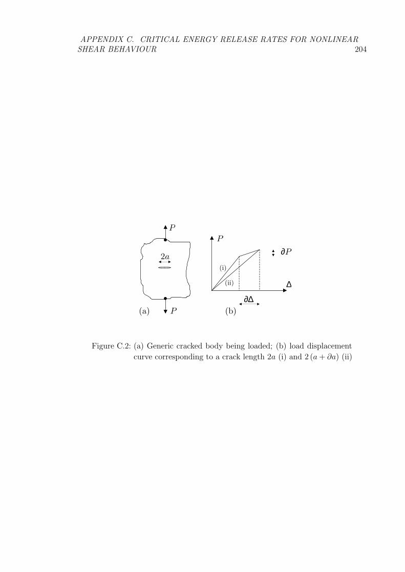
APPENDIX C. CRITICAL ENERGY RELEASE RATES FOR NONLINEAR
SHEAR BEHAVIOUR 204
2a
∂∆
∂P
P
∆
(i )
(i i )
P
P ( a ) ( b )
Figure C.2: (a) Generic cracked body being loaded; (b) load displacement
curve corresponding to a crack length 2a (i) and 2 (a+ ∂a) (ii)

Appendix D
Characteristic lengths for brick
elements
Once the fracture area within an element is known, computing the characteristic
length used in Eqs. 4.31, 4.38 and 4.42 offers no difficulties (L = V/A). However,
given the generic orientation of the fracture plane within an element, computing the
fracture area is not trivial, even for rectangular brick elements and assuming that
the fracture plane passes at the integration point in the centre of the element.
The heuristic proposed here is only approximate. The element dimensions L1,
L2 and L3 are obtained from the nodal coordinates within the material subroutine.
Fig. D.1(a) shows the rotation from the element axes (1, 2, 3) to the material axes
(a, b, c). The rotation from the material axes to a matrix fracture plane is shown
in Fig. D.1(b). From Figs. D.1(a) and (b), the fracture area for matrix failure is
A = LaLcφ and the characteristic length is
Lmat =L1L2L3
LaLcφ(D.1)
with La and Lcφ given in Figs. D.1(a) and (b).
For fibre kinking, the rotation to the kinking plane is shown in Fig. D.1(c) and
to the misaligned frame in Fig. D.1(d). The characteristic length for fibre-kinking
comes then as
Lkink =L1L2L3
LamLcψ(D.2)
205

APPENDIX D. CHARACTERISTIC LENGTHS FOR BRICK ELEMENTS 206
1
a
b 2L
1L
2
��
β
3
21
21
/
sin,
cosmin
������
���
���
�
==
� ��
�=ββ �
��� �=φφφ
sin,
cosmin ���
���b
��
��
c
φ��
φ
ψψ
ψ ψψ����
�������
���/
sin,
cosmin
=
� ��
� !=
b
"#
$%
c
ψ&'
ψ
ψ(ψ)
* +,
-. /=θθψ
sin,
cosmin 011
22243a
56
78
9:;
θ<=>?ψ@
( a ) ( b ) ( c ) ( d )
Figure D.1: Determination of the characteristic length within an element:
(a) rotation of an angle β; (b) rotation of an angle φ; (c) rotation
of an angle ψ and (d) rotation of an angle θ
with Lam and Lcψ obtained from Figs. D.1(a), (b) and (c). For fibre tensile failure,
the fracture plane is normal to the fibres and thus
Lft = La (D.3)
with La given in Fig. D.1(a).

Bibliography
[1] Livermore Software Technology Corporation, California, USA, LS-Dyna 970
(2003).
[2] A. Puck, H. Schurmann, Failure analysis of FRP laminates by means of physi-
cally based phenomenological models, Composites Science and Technology 58
(1998) 1045–1067.
[3] A. S. Argon, Fracture of composites, in: Treatise on Materials Science and
Technology, Academic Press, New York, 1972, pp. 79–114.
[4] C. G. Davila, N. Jaunky, S. Goswami, Failure criteria for FRP laminates in
plane stress, in: 44th AIAA/ ASME/ ASCE/ AHS/ ASC Structures, Struc-
tural Dynamics, and Materials Conference, 2003, AIAA Paper 2003-1991.
[5] M. F. S. F. de Moura, J. P. Goncalves, A. T. Marques, P. T. de Castro,
Prediction of compressive strength of carbon-epoxy laminates containing de-
laminations by using a mixed-mode damage model, Composite Structures 50
(2000) 151–157.
[6] P. P. Camanho, C. G. Davila, Mixed-mode decohesion finite elements for the
simulation of delamination in composite materials, Tech. Rep. NASA/TM-
2002-211737, National Aeronautics and Space Administration, U. S. A. (2002).
[7] Y. Mi, M. A. Crisfield, Analytical derivation of load/ displacement relationship
for the DCB and MMB and proof of the FEA formulation, Tech. rep., Internal
Report, Department of Aeronautics, Imperial College London (April 1996).
207

BIBLIOGRAPHY 208
[8] O. Allix, A. Corigliano, Geometrical and interfacial non-linearities in the anal-
ysis of delamination in composites, International Journal of Solids and Struc-
tures 36 (1999) 2189–2216.
[9] M. Ortiz, A. Pandolfi, Finite-deformation irreversible cohesive elements for
three-dimensional crack-propagation analysis, International Journal for Nu-
merical Methods in Engineering 44 (1999) 1267–1282.
[10] P. P. Camanho, C. G. Davila, M. F. de Moura, Numerical simulation of mixed-
mode progressive delamination in composite materials, Journal of Composite
Materials 37 (16) (2003) 1415–1438.
[11] Y. Mi, M. A. Crisfield, A. O. Davies, Progressive delamination using interface
elements, Journal of Composite Materials 32 (14) (1998) 1246–1272.
[12] Y. Qiu, M. A. Crisfield, G. Alfano, An interface element formulation for the
simulation of delamination with buckling, Engineering Fracture Mechanics 68
(2001) 1755–1776.
[13] S. T. Pinho, P. P. Camanho, M. F. de Moura, Numerical simulation of the
crushing process of composite materials, International Journal of Crashwor-
thiness 9 (3) (2004) 263–276.
[14] M. R. Wisnom, Modelling the effect of cracks on interlaminar shear strength,
Composites Part A 27 (1996) 17–24.
[15] A. F. Johnson, A. K. Pickett, P. Rozycki, Computational methods for predict-
ing impact damage in composite structures, Composites Science and Technol-
ogy 61 (2001) 2183–2192.
[16] A. K. Pickett, Review of finite element simulation methods applied to man-
ufacturing and failure prediction in composite structures, Applied Composite
Materials 9 (2002) 43–58.

BIBLIOGRAPHY 209
[17] R. Borg, L. Nilsson, K. Simonsson, Simulation of felamination in fiber compos-
ites with a discrete cohesive failure model, Composites Science and Technology
61 (2001) 667–677.
[18] R. Borg, L. Nilsson, K. Simonsson, Modeling of delamination using a dis-
cretized cohesive zone and damage formulation, Composites Science and Tech-
nology 62 (2002) 1299–1314.
[19] R. Borg, L. Nilsson, K. Simonsson, Simulating DCB, ENF and MMB exper-
iments using shell elements and a cohesive zone model, Composites Science
and Technology 64 (2004) 269–278.
[20] R. Borg, L. Nilsson, K. Simonsson, Simulation of low velocity impact on fiber
laminates using a cohesive zone based delamination model, Composites Science
and Technology 64 (2004) 279–288.
[21] G. Alfano, M. A. Crisfield, Finite element interface models for the delamina-
tion analysis of laminated composites: mechanical and computational issues,
International Journal for Numerial Methods in Engineering 50 (2001) 1701–
1736.
[22] O. Allix, A. Corigliano, Modeling and simulation of crack propagation in
mixed-mode interlaminar fracture specimens, International Journal of Frac-
ture 77 (1996) 111–140.
[23] M. F. S. F. de Moura, J. P. Goncalves, A. T. Marques, P. T. de Castro,
Elemento finito isoparametrico de interface para problemas tridimensionais,
Revista Internacional de Metodos Numericos Para Calculo e Diseno en Inge-
nierıa 14 (1996) 447–466.
[24] P. P. Camanho, M. F. de Moura, Simulation of interlaminar damage using de-
cohesion elements, in: 13th International Conference on Composite Materials,
Beijing, China, 2001.
[25] C. G. Davila, P. P. Camanho, M. F. de Moura, Mixed-mode decohesion el-
ements for analyses of progressive delamination, in: 42nd AIAA/ ASME/

BIBLIOGRAPHY 210
ASCE/ AHS/ ASC Structures, Structural Synamics, and Materials Confer-
ence and Exhibit, Seattle, 2001.
[26] M. L. Benzeggagh, M. Kenane, Measurement of mixed-mode delamination
fracture toughness of unidirectional glass/epoxy composites with mixed-mode
bending apparatus, Composites Science and Technology 56 (4) (1996) 439–449.
[27] V. Tvergaard, Effect of fibre debonding in a whisker-reinforced metal, Mate-
rials Science and Engineering A 125 (1990) 203–213.
[28] V. K. Goyal, E. R. Johnson, An irreversible constitutive law for modeling
the delamination process using interface elements, in: 43rd AIAA/ ASME/
ASCE/ AHS/ ASC Structures, Structural Dynamics, and Materials Confer-
ence and Exhibit, 2002.
[29] J. G. Williams, H. Hadavinia, Analytical solutions for cohesive zone models,
Journal of the Mechanics and Physics of Solids 50 (2002) 809–825.
[30] ASTM standard D 5528-94a, Standard test method for mode I interlaminar
fracture touthness of unidirectional fiber-reinforced polymer matrix compos-
ites (1994).
[31] R. H. Martin, T. Elms, S. Bowron, Characterisation of mode II delamination
using the 4ENF, in: I. of Materials London (Ed.), 4th European Conference
on Composites: Testing and Standardisation, Lisbon, Portugal, 1998.
[32] R. H. Martin, B. D. Davidson, Mode II fracture toughness evaluation using
four point bend, end notched flexure test, Plastics, Rubber and Composites
28 (8) (1999) 401–406.
[33] ASTM Standard D6671-01, Standard test method for mixed mode I-mode
II interlaminar fracture toughness of unidirectional fiber reinforced polymer
matrix composites (2001).
[34] G. A. O. Davies, P. Robinson, Predicting failure by debonding delaminations,
in: Debonding / Delamination of Composites, AGARD-CP-530, Advisory

BIBLIOGRAPHY 211
Group for Aerospace Research and Development, Neuilly Sur Seine, France,
1992, pp. 5.1–5.27.
[35] S. T. Pinho, L. Iannucci, P. Robinson, Modelling delamination in an explicit
FE code using 3D decohesion elements, in: Composites Testing and Model
Identification, CompTest2004, Bristol, U.K., 21st-23rd September 2004.
[36] S. T. Pinho, L. Iannucci, P. Robinson, Physically-based failure models and
criteria for laminated fibre-reinforced composites. Development and Imple-
mentation, Tech. Rep. 04-02, Department of Aeronautics, Imperial College
London (2004).
[37] S. T. Pinho, L. Iannucci, P. Robinson, Physically-based failure models and cri-
teria for laminated fibre-reinforced composites with emphasis on fibre-kinking.
Part I: Development, In press, Composites: Part A (2005).
[38] S. T. Pinho, L. Iannucci, P. Robinson, Physically-based failure models and cri-
teria for laminated fibre-reinforced composites with emphasis on fibre-kinking.
Part II: FE implementation, Accepted for publication, Composites: Part A.
[39] C. G. Davila, P. P. Camanho, Failure criteria for FRP laminates in plane
stress, Tech. Rep. NASA/TM-2003-212663, National Aeronautics and Space
Administration, U. S. A. (2003).
[40] S. T. Pinho, P. P. Camanho, C. G. Davila, L. Iannucci, P. Robinson, Failure
models and criteria for FRP in plane or 3D stress state including shear nonlin-
earity, Tech. Rep. NASA/ TM-2005-213530, National Aeronautics and Space
Administration, U. S. A. (2005).
[41] C. G. Davila, P. P. Camanho, Physically based failure criteria for transverse
matrix cracking, in: 9th Portuguese Conference on Fracture, 2004.
[42] M. J. Hinton, P. G. Soden, A comparison of the predictive capabilities of
current failure theories for composite laminates, judged against experimental
evidence, Composites Science and Technology 62 (2002) 1725–1797.

BIBLIOGRAPHY 212
[43] P. D. Soden, M. J. Hinton, A. S. Kaddour, Biaxial test results for strength and
deformation of a range of e-glass and carbon fibre reinforced composite lami-
nates: Failure exercise benchmark data, Composites Science and Technology
62 (2002) 1489–1514.
[44] A. Puck, Calculating the strength of glass fibre/plastic laminates under com-
bined load, Kunststoffe, German Plastics 55 (1969) 18–19, german text pp.
780-787.
[45] A. Puck, W. Schneider, On failure mechanisms and failure criteria of filament-
wound glass-fibre/resin composites, Plastics and Polymers (1969) 33–44.
[46] A. Puck, H. Schurmann, Failure analysis of FRP laminates by means of physi-
cally based phenomenological models, Composites Science and Technology 62
(2002) 1633–1662.
[47] G. J. Dvorak, N. Laws, Analysis of progressive matrix cracking in composite
laminates II. First ply failure, Journal of Composite Materials 21 (1987) 309–
329.
[48] J. Echabi, F. Trochu, R. Gauvin, Review of failure criteria of fibre composite
materials, Polymer Composites 17 (6) (1996) 786–798.
[49] F. Paris, A study of failure criteria of fibrous composite materials, Tech. Rep.
NASA/CR-2001-210661, National Aeronautics and Space Agency (2001).
[50] S. W. Tsai, Strength characterisation of composite materials, Tech. Rep.
NASA CR-224, National Aeronautics and Space Agency (1965).
[51] S. W. Tsai, E. M. Wu, A general theory of strength for anisotropic materials,
Journal of Composite Materials 5 (1971) 58–80.
[52] O. Hoffman, The brittle strenght of orthotropic materials, Journal of Com-
posite Materials 1 (1967) 200–206.

BIBLIOGRAPHY 213
[53] M. Nahas, Survey of failure and post-failure theories of laminated fiber-
reinforced composites, Jounal of Composites Technology and Research 8
(1994) 138–153.
[54] Z. Hashin, A. Rotem, A fatigue failure criterion for fibre reinforced materials,
Journal of Composite Materials 7 (1973) 448–464.
[55] Z. Hashin, Failure criteria for unidirectional fibre composites, Journal of Ap-
plied Mechanics 47 (1980) 329–334.
[56] S. E. Yamada, C. T. Sun, Analysis of laminate strength and its distribution,
Journal of Composite Materials 12 (1978) 275–284.
[57] F.-K. Chang, M. H. Chen, The in situ ply shear strength distributions in
Graphite/Epoxy laminated composites, Journal of Composite Materials 21
(1987) 708–733.
[58] F.-K. Chang, K.-Y. Chang, Post-failure analysis of bolted composite joints in
tension or shear-out mode failure, Journal of Composite Materials 21 (1987)
809–833.
[59] F.-K. Chang, K.-Y. Chang, A progressive damage model for laminated com-
posites containing stress concentration, Journal of Composite Materials 21
(1987) 834–855.
[60] R. M. Christensen, Stress based Yield/Failure criteria for fiber composites,
Journal of Solids and Structures 34 (5) (1997) 529–543.
[61] A. Puck, Failure analysis for FRP. Models for use in practice, Hanser, Munich,
Viena. Original in German (1996).
[62] J. Kopp, W. Michaeli, Dimensioning of thick laminates using new IFF strength
criteria and some experiments for their verification, Proceedings of the ESA
ESTEC Conference (1996) 305–312.
[63] L. Kroll, W. Hufenbach, Physically based failure criterion for dimensioning of
thick-walled laminates, Applied Composite Materials 4 (1997) 321–332.

BIBLIOGRAPHY 214
[64] L. J. Hart-Smith, A new approach to fibrous composite laminate strength
prediction, Eighth DOD/NASA/ FAA Conference on Fibrous Composites in
Structural Design, NASA CP-3087, Part 2 (1989) 663–693.
[65] L. J. Hart-Smith, Should fibrous composite failure modes be interacted or
superimposed?, Composites 24 (1993) 53–55.
[66] M. J. Hinton, P. G. Soden, Predicting failure in composite laminates: the
background to the exercise, Composites Science and Technology 58 (1998)
1001–1010.
[67] L. J. Hart-Smith, Prediction of the original and truncated maximum-strain
failure models for certain fibrous composite laminates, Composites Science
and Technology 58 (7) (1998) 1151–1178.
[68] L. J. Hart-Smith, Predictions of a generalized maximum-shear-stress failure
criterion for certain fibrous composite laminates, Composites Science and
Technology 58 (7) (1998) 1179–1208.
[69] L. J. Hart-Smith, Comparison between theories and test data concerning the
strength of various fibre-polymer composites, Composites Science and Tech-
nology 62 (2002) 1591–1618.
[70] P. K. Gotsis, C. C. Chamis, L. Minnetyan, Prediction of composite laminate
fracture: micromechanics and progressive fracture, Composites Science and
Technology 58 (7) (1998) 1137–1149.
[71] P. K. Gotsis, C. C. Chamis, L. Minnetyan, Application of progressive fracture
analysis for predicting failure envelopes and stressstrain behaviors of composite
laminates: A comparison with experimental results, Composites Science and
Technology 62 (2002) 1545–1559.
[72] L. N. McCartney, Predicting transverse crack formation in cross-ply laminates,
Composites Science and Technology 58 (7) (1998) 1069–1081.

BIBLIOGRAPHY 215
[73] L. N. McCartney, Prediction of ply crack formation and failure in laminates,
Composites Science and Technology 62 (2002) 1619–1631.
[74] A. Rotem, Prediction of laminate failure with the rotem failure criterion, Com-
posites Science and Technology 58 (7) (1998) 1083–1094.
[75] A. Rotem, The rotem failure criterion: Theory and practice, Composites Sci-
ence and Technology 62 (2002) 1663–1671.
[76] C. T. Sun, J. Tao, Prediction of failure envelopes and stress/strain behaviour of
composite laminates, Composites Science and technology 58 (7) (1998) 1125–
1136.
[77] C. T. Sun, J. Tao, A. S. Kaddour, The prediction of failure envelopes and
stress/strain behavior of composite laminates: Comparison with experimental
results, Composites Science and Technology 62 (2002) 1673–1682.
[78] C. T. Sun, B. J. Quinn, D. W. Oplinger, Comparative evaluation of failure
analysis methods for composite laminates, DOT/FAA/AR (1996) 95–109.
[79] K.-S. Liu, S. W. Tsai, A progressive quadratic failure criterion for a laminate,
Composites Science and Technology 58 (7) (1998) 1023–1032.
[80] W. E. Wolfe, T. S. Butalia, A strain-energy based failure criterion for non-
linear analysis of composite laminates subjected to biaxial loading, Composites
Science and Technology 58 (7) (1998) 1107–1124.
[81] T. S. Butalia, W. E. Wolfe, A strain-energy-based non-linear failure criterion:
Comparison of numerical predictions and experimental observations for sym-
metric composite laminates, Composites Science and Technology 62 (2002)
1697–1710.
[82] E. C. Edge, Stress-based grant-sanders method for predicting failure of com-
posite laminates, Composites Science and Technology 58 (7) (1998) 1033–1041.
[83] E. C. Edge, A comparison of theory and experiment for the stress-based grant-
sanders method, Composites Science and Technology 62 (2002) 1571–1589.

BIBLIOGRAPHY 216
[84] P. A. Zinoviev, S. V. Grigoriev, O. V. Lebedeva, L. P. Tairova, The strength
of multilayered composites under a plane-stress state, Composites Science and
Technology 58 (7) (1998) 1209–1223.
[85] P. A. Zinoviev, O. V. Lebedeva, L. P. Tairova, A coupled analysis of exper-
imental and theoretical results on the deformation and failure of composite
laminates under a state of plane stress, Composites Science and Technology
62 (2002) 1711–1723.
[86] Z.-M. Huang, A bridging model prediction of the ultimate strength of compos-
ite laminates subjected to biaxial loads, Composites Science and Technology
64 (2004) 395–448.
[87] Z.-M. Huang, Correlation of the bridging model predictions of the biaxial
failure strengths of fibrous laminates with experiments, Composites Science
and Technology 64 (2004) 529–548.
[88] J. S. Mayes, A. C. Hansen, Composite laminate failure analysis using multi-
continuum theory, Composites Science and Technology 64 (2004) 379–394.
[89] J. S. Mayes, A. C. Hansen, A comparison of multicontinuum theory based fail-
ure simulation with experimental results, Composites Science and Technology
64 (2004) 517–527.
[90] R. G. Cuntze, A. Freund, The predictive capability of failure mode concept-
based strength criteria for multidirectional laminates, Composites Science and
Technology 64 (2004) 343–377.
[91] R. G. Cuntze, The predictive capability of failure mode concept-based strength
criteria for multi-directional laminates—part B, Composites Science and Tech-
nology 64 (2004) 487–516.
[92] P. D. Soden, M. J. Hinton, A. S. Kaddour, Lamina properties, lay-up con-
figurations and loading conditions for a range of fibre-reinforced composite
laminates, Composites Science and Technology 58 (1998) 1011–1022.

BIBLIOGRAPHY 217
[93] A. Parvizi, K. Garrett, J. Bailey, Constrained cracking in glass fibre-reinforced
epoxy cross-ply laminates, Journal of Material Science 13 (1978) 195–201.
[94] A. S. D. Wang, Fracture mechanics of sublaminate cracks in composite mate-
rials, Composites Technology Review 6 (2) (1984) 45–62.
[95] I. Shahid, F. K. Chang, An accumulative damage model for tensile and shear
failures of laminated composite plates, Journal of Composite Materials 29
(1995) 926–981.
[96] S. C. Tan, R. J. Nuismer, A theory for progressive matrix cracking in composite
laminates, Journal of Composite Materials 23 (1989) 1029–1047.
[97] R. Talreja, Transverse cracking and stiffness reduction in composite laminates,
Journal of Composite Materials 19 (1985) 355–375.
[98] D. H. Allen, C. E. Harris, S. E. Groves, A thermomechanical constitutive
theory for elastic composites with distributed damage- I. Theoretical develop-
ments, International Journal of Solids and Structures 23 (9) (1987) 1301–1318.
[99] D. H. Allen, C. E. Harris, S. E. Groves, A thermomecanical constitutive the-
ory for elastic composites with distributed damage- II. Application to matrix
cracking in laminated composites, International Journal of Solids and Struc-
tures 23 (9) (1987) 1319–1338.
[100] R. Talreja, S. Yalvac, L. D. Yats, D. G. Wetters, Transverse cracking and
stiffness reduction in cross ply laminates of different matrix toughness, Journal
of Composite Materials 26 (11) (1992) 1644–1663.
[101] D. L. Flaggs, K. M. H, Experimental determination of the in situ transverse
lamina strength in graphite/epoxy laminates, Journal of Composite Materials
16 (1982) 103–116.
[102] N. Laws, G. J. Dvorak, Progressive transverse cracking in composite laminates,
Journal of Composite Materials 22 (1988) 900–919.

BIBLIOGRAPHY 218
[103] J. Li, J. K. Sen, Analysis of frame-to-skin joint pull-off tests and prediction
of the delamination failure, in: 42nd AIAA/ASME/ASCE/AHS/ASC Struc-
tures, Structural Dynamics and Materials Conference, Seattle, WA, USA,
2000.
[104] J. Li, Three-dimensional effects in the prediction of flange delamination in
composite skin-stringer pull-off specimens, in: 15th Conference of the Ameri-
can Society for Composites, Texas, USA, 2000.
[105] H. T. Hahn, T. Johannesson, Fracture of unidirectional composites: Theory
and applications, in: G. J. Dvorak (Ed.), Mechanics of Composite Materials,
AMD, 1983, pp. 135–142.
[106] E. M. Wu, R. C. J. Reuter, Crack extension in fiberglass reinforced plastics
and a critical examination of the general fracture criterion. Theoretical and
applied mechanics report no. 275, University of Illinois (1965).
[107] R. S. Sandhu, Nonlinear response of unidirectional and angle-ply laminates,
in: AIAA Paper No. 74-380, 15th AIAA-ASME Structural Dynamics and
Materials Conference, Las Vegas, Nevada, 1974.
[108] F.-K. Chang, R. A. Scott, Failure strength of nonlinearly elastic composite
laminates containing a pin loaded hole, Journal of Composite Materials 18
(1984) 464–477.
[109] H. Tada, P. C. Paris, G. R. Irwin, The Stress Analysis of Cracks Handbook,
3rd. Ed., American society of Mechanical Engineers, New York, 2000.
[110] H. T. Hahn, S. W. Tsai, Nonlinear elastic behavior of unidirectional composite
laminae, Journal of Composite Materials 7 (1973) 102–118.
[111] D. Leguillon, Strength or toughness? A criterion for crack onset at a notch,
European Journal of Mechanics - A/Solids 21 (1) (2002) 61–72.

BIBLIOGRAPHY 219
[112] C. R. Schultheisz, A. M. Waas, Compressive failure of composites, part I: Test-
ing and micromechanical theories, Progress in Aerospace Sciences 32 (1996)
1–42.
[113] V. W. Rosen, Mechanics of composite strengthening, Fiber Composite Mate-
rials American Society of Metals, Metals Park, Ohio (1965) 37–75.
[114] H. Schuerch, Prediction of compressive strength in uniaxial boron fiber-metal
matrix composite materials, AIAA Journal 4 (1) (1966) 102–106.
[115] L. B. Greszczuk, Microbuckling of unidirectional composites, Tech. Rep. Air
Force Materials Laboratory Technical Report, OHAFML-TR-71-231, Wright-
Patterson Air Force Base, OH (1972).
[116] L. B. Greszczuk, Failure mechanics of composites subjected to compressive
loading, Tech. Rep. Air Force Materials Laboratory Technical Report, AFML-
TR-72-107, Wright-Patterson Air Force Base, OH (1972).
[117] L. B. Greszczuk, Microbuckling of lamina reinforced composites, in: Com-
posite materials: Testing and Design (Third Conference), ASTM STP 546,
American Society for Testing and Materials, Philadelphia, 1974, pp. 5–29.
[118] L. B. Greszczuk, Microbuckling failure of circular fiber-reinforced composites,
AIAA Journal 13 (10) (1975) 1311–1318.
[119] J. R. Lager, R. R. June, Compressive strength of boron-epoxy composites,
Journal of Composite Materials 3 (1969) 48–56.
[120] M. E. de Ferran, B. Harris, Compression strength of polyester resin reinforced
with steel wires, Journal of Composite Materials 4 (1970) 62–72.
[121] D. Purslow, R. T. Potter, The effect of environment on the compression
strength of notched CFRP / a fractografic investigation, Composites 15 (2)
(1984) 112–120.

BIBLIOGRAPHY 220
[122] A. M. Waas, C. D. J. Babcock, W. G. Knauss, An experimental study of com-
pression failure of fibrous laminated composites in the presence of stress gra-
dients, International Journal of Solids and Structures 26 (9-10) (1990) 1071–
1098.
[123] J. G. Davis Jr, Compressive strength of fiber-reinforced composite materials,
in: Composite Reliability, ASTM STP 580, Americal Society for Testing and
Materials, Philadelphia, 1975, pp. 364–377.
[124] M. J. Shuart, Failure of compression-loaded multidirectional composite lami-
nates, AIAA Journal 27 (1989) 1274–1279.
[125] M. J. Shuart, Short-wavelength buckling and shear failures for compression-
loaded composite laminates, Tech. Rep. NASA Technical Memorandum, TM-
87640, NASA (1985).
[126] J. C. Grandidier, M. Potier-Ferry, Microbuckling and homogenization for long
fiber composites, Zeitschrift fur Angewandte Mathematik und Mechanik 71 (4)
(1991) T371–T374.
[127] A. Agah-Tehrani, S. Gunawardena, Micro- and macrobifurcation of fibrous
metal-matrix composites under uniaxial compression, Journal of the Mechan-
ics and Physics of Solids 39 (1991) 1073–1103.
[128] S. R. Swanson, A micro-mechanical model for in-situ compression strength of
fiber composite laminates, Transactions of the American Society of Mechanical
Engineers. Series H, Journal of Engineering Materials and Technology 114
(1992) 8–12.
[129] I. G. Tadjbakhsh, Y. M. Wang, Fiber buckling in three-dimensional periodic-
array composites, International Journal of Solids and Structures 29 (1992)
3169–3183.
[130] C. R. Chaplin, Compressive fracture in unidirectional glass-reinforced plastics,
Journal of Materials Science 12 (1977) 347–352.

BIBLIOGRAPHY 221
[131] R. R. Effendi, J. J. Barrau, D. Guedra-Degeorges, Failure mechanism analysis
under compression loading of unidirectional carbon/epoxy composites using
micromechanical modelling, Composite Structures 31 (2) (1995) 87–98.
[132] H. T. Hahn, M. M. Sohi, Buckling of a fiber bundle embedded in epoxy,
Composites Science and Technology 27 (1986) 25–41.
[133] M. R. Piggott, B. Harris, Compression strength of carbon, glass and kevlar-
49 fibre reinforced polyester resins, Journal of Materials Science 15 (1980)
2523–2538.
[134] M. R. Piggott, A theoretical framework for the compressive properties of
aligned fibre composites, Journal of Materials Science 16 (1981) 2837–2845.
[135] B. Budiansky, Micromechanics, Computers and Structures 16 (1983) 3–12.
[136] B. Budiansky, N. A. Fleck, Compressive failure of fibre composites, Journal of
the Mechanics and Physics of Solids 41 (1) (1993) 183–211.
[137] B. Budiansky, N. A. Fleck, J. C. Amazigo, On kink-band propagation in fiber
composites, Journal of the mechanics and physics of solids 46 (9) (1998) 1637–
1653.
[138] S. Kyriakides, R. Arseculeratne, E. J. Perry, On the compressive failure of fiber
reinforced composites, International Journal of Solids and Structures 32 (6/7)
(1995) 689–738.
[139] T. J. Vogler, S. Kyriakides, Initiation and axial propagation of kink bands in
fiber composites, Acta Materialia 45 (6) (1997) 2443–2454.
[140] T. J. Vogler, S. Kyriakides, On the axial propagation of kink bands in fiber
composites: Part i experiments, International Journal of Solids and Structures
36 (1999) 557–574.
[141] A. S. Wronsky, T. V. Parry, Compressive failure and kinking in uniaxially
aligned glass-resin composite under superposed hydrostatic pressure, Journal
of Materials Science 17 (1982) 3656–3662.

BIBLIOGRAPHY 222
[142] P. Ladeveze, E. le Dantec, Damage modeling of the elementary ply for lami-
nated composites, Composites Science and Technology 43 (1992) 257–67.
[143] D. Coutellier, P. Rozycki, Multi-layered multi-material finite element for crash-
worthiness studies, Composites: Part A 31 (2000) 841–851.
[144] A. F. Johnson, Modelling fabric reinforced composites under impact loads,
Composites: Part A 32 (2001) 1197–1206.
[145] A. Matzenmiller, J. Lubliner, R. L. Taylor, A constitutive model for
anisotropic damage in fiber-composites, Mechanics of Materials 20 (2) (1995)
125–152.
[146] K. V. Williams, R. Vaziri, Application of a damage mechanics model for pre-
dicting the impact response of composite materials, Computers and Structures
70 (2001) 997–1011.
[147] K. V. Williams, R. Vaziri, A. Poursartip, A physically based continuum dam-
age mechanics model for thin laminated composite structures, International
Journal of Solids and Structures 40 (9) (2003) 2267–2300.
[148] M. G. D. Geers, Experimental analysis and computational modelling of dam-
age and fracture, Technishe Universiteit Eindhoven, Eindhoven, 1997.
[149] S. Pietruszczak, Z. Mro, Finite element analysis of deformation of quasi-brittle
fracture using damaging cohesive surfaces, International Journal for Numerical
Methods in Engineering 17 (1981) 327–334.
[150] Z. P. Bazant, B. Oh, Crack band theory for fracture of concrete.materiaux et
constructions, Materials and Structures 16 (93) (1983) 155–177.
[151] E. Van der Giessen, R. de Borst, Material Instabilities in Solids, John Wiley
and Sons Ltd, 1998.
[152] C. Soutis, P. T. Curtis, A method for predicting the fracture toughness of
CFRP laminates failing by fibre microbuckling, Composites Part A 31 (2000)
733–740.

BIBLIOGRAPHY 223
[153] ASTM Standard D3518/D3518M(2001), Standard test method for in-plane
shear reponse of polymer matrix composite materials by tensile test of a +/-
45 laminate (2001).
[154] M. P. F. Sutcliffe, N. A. Fleck, Microbuckle propagation in fibre composites,
Acta Materialia 45 (3) (1997) 921–932.
[155] P. M. Moran, C. F. Shih, Kink band propagation and broadening in ductile
matrix fiber composites: experiments and analysis, International Journal of
Solids and Structures 35 (15) (1998) 1709–1722.
[156] A. J. Davies, Crashworthiness of composite sandwich structures, Ph.D. thesis,
Department of Aeronautics, Imperial College London (2002).
[157] A. C. Garg, Intralaminar and interlaminar fracture in graphite/epoxy lami-
nate, Engineering fracture mechanics 23 (4) (1986) 719–733.
[158] D. R. Leach, J. C. Seferis, Intrinsic characterization of continuous fibre re-
inforced thermoplastic composites—1: Toughness characterization of car-
bon fibre/ polyether ether ketone (CF/PEEK) laminates, Pure and Applied
Chemestry 63 (11) (1991) 1609–1625.
[159] K. D. Cowley, P. W. R. Beaumont, The interlaminar and intralaminar frac-
ture toughness of carbon-fibre/polymer composites: The effect of temperature,
Composite Science and Technology 57 (1997) 1433–1444.
[160] R. W. Truss, P. J. Hine, R. A. Duckett, Interlaminar and intralaminar frac-
ture toughness of uniaxial continuous and discontinuous carbon fibre/epoxy
composites, Composites Part A 28A (1997) 627–636.
[161] S. Jose, R. K. Kuma, M. K. Jana, G. V. Rao, Intralaminar fracture toughness
of a cross-ply laminate and its constituent sub-laminates, Composites Science
and Technology 61 (8) (2001) 1115–1122.
[162] D. C. Leach, D. R. Moore, The toughness of aromatic polymer composites,
Composites Science and Technology 23 (1985) 131–161.

BIBLIOGRAPHY 224
[163] U. Hansen, J. W. Gillespie Jr, Dependence of intralaminar fracture tough-
ness on direction of crack propagation in unidirctional composites., Jounal of
Composites Technology and Research 20 (2) (1998) 89–99.
[164] M. Vernon, An investigation into the use of edge delaminations for interlaminar
fracture, Master’s thesis, Centre for Composite Materials, Imperial College of
Science, Technology and Medicine (2001).
[165] C. Fensome, Development of a test method for the measurement of intralami-
anr fracture toughness of unidirectional lamianted composites, Master’s thesis,
Centre for Composite Materials, Imperial College of Science, Technology and
Medicine (2002).
[166] M. Iwamoto, Q. Q. Ni, T. Fujiwara, K. Kurashiki, Intralaminar fracture mech-
anism in unidirectional CFRP composites. Part I: Intralaminar toughness and
AE characteristics, Engineering Fracture Mechanics 64 (1999) 721–745.
[167] K. Humer, E. K. Tschegg, S. M. Spiebberger, H. W. Weber, Fracture me-
chanical characterisation of fibre reinforced plastics in the intralaminar crack
opening mode (mode I) and in the shear mode (mode II), Cryogenics 38 (1998)
69–74.
[168] P. J. Iglesias, Measuring the resistance to through thickness crack growth,
Exchange project, Department of Aeronautics, Imperial College of Science,
Technology and Medicine (March 2002).
[169] K. Zi, Intralaminar fracture transverse to the fibre direction in unidirectional
composite materials, Exchange project, Department of Aeronautics, Imperial
College of Science, Technology and Medicine (2002).
[170] D. P. Rooke, D. J. Cartwright, Compendium of Stress Intensity Factors, Lon-
don HMSO, 1976.
[171] C. Soutis, N. A. Fleck, P. A. Smith, Failure prediction technique for com-
pression loaded carbon fibre-epoxy laminate with an open hole, Journal of
Composite Materials 25 (1991) 1476–1498.

BIBLIOGRAPHY 225
[172] C. Soutis, P. T. Curtis, N. A. Fleck, Compressive failure of notched carbon
fibre composites, Proceedings of the Royal Society London A 440 (1993) 241–
256.
[173] J. Ratcliffe, W. Jackson, J. Schaff, Compression strength prediction of impact-
damaged composite sandwich panels, in: American Helicopter Society 60th
Annual Forum, Baltimore, MD, 2004.
[174] W. C. Jackson, J. G. Ratcliffe, Measurement of fracture energy for kink-band
growth in sandwich specimens (paper no. 24), in: Composites Testing and
Model Identification, CompTest2004, University of Bristol, Bristol, UK, 2004.
[175] Standard Test Method for Plane-Strain Fracture Toughness of Metallic Mate-
rials, ASTM E399-90, Annual Book of ASTM Standards 03.01 (1993) 407–528.
[176] P. C. Paris, G. C. Sih, Stress analysis of cracks, fracture toughness and appli-
cations, STP-381, ASTM (1969) 30–83.
[177] Abaqus, Inc., 1080 Main Street, Pawtucket, R. I. 02860, Abaqus 6.4-1 (2003).
[178] J. G. Haberle, The imperial college method for testing composite materials in
compression, Technical Memo TM 99/03. Imperial College of Science, Tech-
nology and Medicine, Centre for Composite Materials. Edited by E W Godwin
(1999).
[179] ASTM Standard D3410/3410M-95, Standard test method for compressive
properties of polymer matrix composite materials with unsupported gage sec-
tion by shear loading (1995).
[180] ASTM Standard D3039/D3039M-00, Standard test method for tensile prop-
erties of polymer matrix composite materials (2000).
[181] ASTM Standard D 5379, Shear properties of composite materials by the V-
notched beam method (1993).
[182] ASTM Standard D 4255, Inplane shear properties of composites laminates
(1983).

BIBLIOGRAPHY 226
[183] ASTM Standard D 7078-05, Shear properties of composite materials by the
V-notched rail shear method (2005).
[184] A. Szekrenyes, Overview on the experimental investigations of the fracture
toughness in composite materials, Hungarian Electronic Journal of Sciences,
Mechanical Engineering and Transport Section (2002) MET–020507–A.
[185] V. Bloodworth, Delamination characteristics of the T300-913 composite ma-
terial under mode I, II and mixed-mode I/II loading, 4th year project report,
Imperial College London (2003).
[186] N. Laws, A note on interaction energies associated with cracks in anisotropic
solids, Philosophical Magazine 36 (2) (1977) 367–372.
[187] J. D. Eshelby, The determination of the elastic field of an ellipsoidal inclusion,
and related problems, Proceedings of the Royal Society A 241 (1957) 376–396.
[188] N. Kinoshita, T. Mura, Elastic fields of inclusions in anisotropic media, Phys-
ica Status Solidi: A 5 (1971) 759–768.
[189] G. Faivre, Heterogeneites ellipsoıdales dans un milieu elastique anisotrope, Le
Journal de Physique 32 (1971) 325–331.
[190] R. S. Rivlin, A. G. Thomas, Rupture of rubber. I. Characteristic energy for
tearing, Journal of Polymer Science 10 (1953) 291–318.