Embed Size (px)
Citation preview
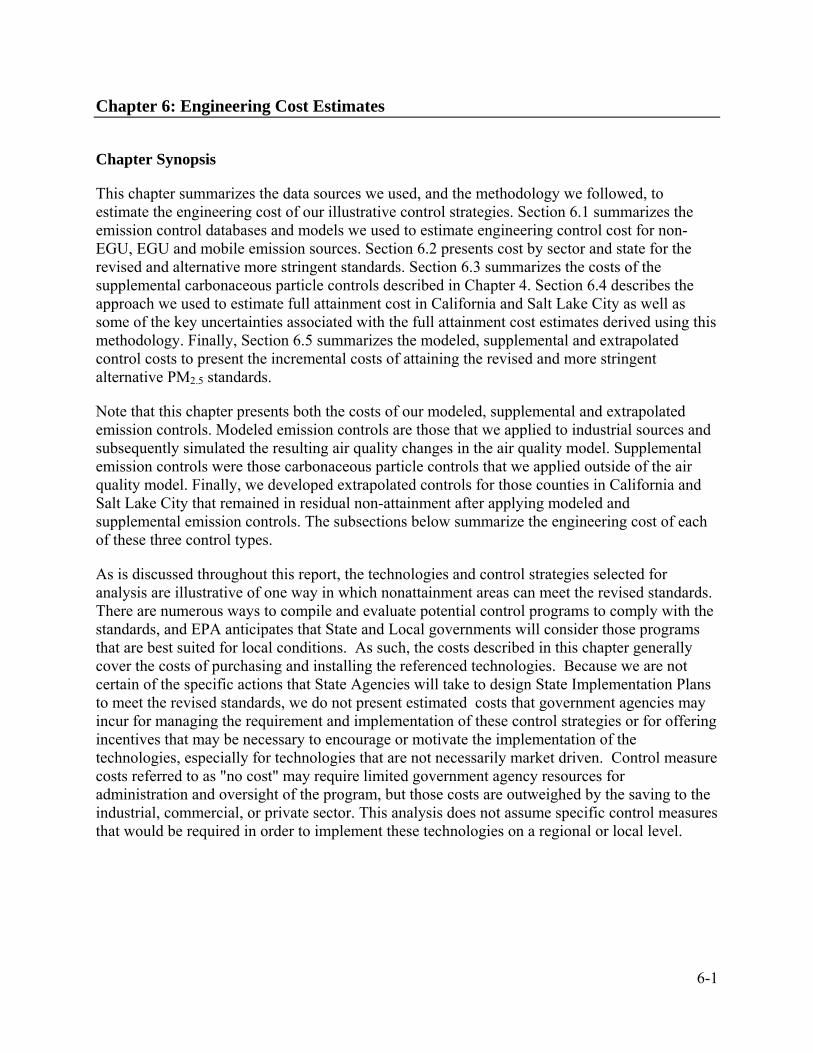
Chapter 6: Engineering Cost Estimates
Chapter Synopsis
This chapter summarizes the data sources we used, and the methodology we followed, to estimate the engineering cost of our illustrative control strategies. Section 6.1 summarizes the emission control databases and models we used to estimate engineering control cost for non-EGU, EGU and mobile emission sources. Section 6.2 presents cost by sector and state for the revised and alternative more stringent standards. Section 6.3 summarizes the costs of the supplemental carbonaceous particle controls described in Chapter 4. Section 6.4 describes the approach we used to estimate full attainment cost in California and Salt Lake City as well as some of the key uncertainties associated with the full attainment cost estimates derived using this methodology. Finally, Section 6.5 summarizes the modeled, supplemental and extrapolated control costs to present the incremental costs of attaining the revised and more stringent alternative PM2.5 standards.
Note that this chapter presents both the costs of our modeled, supplemental and extrapolated emission controls. Modeled emission controls are those that we applied to industrial sources and subsequently simulated the resulting air quality changes in the air quality model. Supplemental emission controls were those carbonaceous particle controls that we applied outside of the air quality model. Finally, we developed extrapolated controls for those counties in California and Salt Lake City that remained in residual non-attainment after applying modeled and supplemental emission controls. The subsections below summarize the engineering cost of each of these three control types.
As is discussed throughout this report, the technologies and control strategies selected for analysis are illustrative of one way in which nonattainment areas can meet the revised standards. There are numerous ways to compile and evaluate potential control programs to comply with the standards, and EPA anticipates that State and Local governments will consider those programs that are best suited for local conditions. As such, the costs described in this chapter generally cover the costs of purchasing and installing the referenced technologies. Because we are not certain of the specific actions that State Agencies will take to design State Implementation Plans to meet the revised standards, we do not present estimated costs that government agencies may incur for managing the requirement and implementation of these control strategies or for offering incentives that may be necessary to encourage or motivate the implementation of the technologies, especially for technologies that are not necessarily market driven. Control measure costs referred to as "no cost" may require limited government agency resources for administration and oversight of the program, but those costs are outweighed by the saving to the industrial, commercial, or private sector. This analysis does not assume specific control measures that would be required in order to implement these technologies on a regional or local level.
6-1

6.1 Data Sources and Methodology
6.1.1 Non-EGU Point and Area Sources: AirControlNET
Once we determined the control technologies selected to meet the standard with the methodology discussed in Chapter 3, we used AirControlNET to estimate engineering control cost. AirControlNET calculates costs using three different methods: (1) by multiplying a dollar per ton estimate against the total tons of a pollutant reduced to derive a total cost estimate; (2) calculating cost by using an equation that incorporates information regarding key plant information; or, (3) both cost per ton and cost equations.1 Most of the control cost information within AirControlNET has been developed as cost per ton inputs. This is likely due to the fact that estimating cost using an equation requires more data and the fact that parameters used in other non-cost per ton methods may not be readily available or broadly representative across sources within the inventory. The costing equations used in AirControlNET require either plant capacity or stack flow to determine annual, capital and/or Operating and Maintenance costs. Capital costs are converted to annual costs, in dollars per ton, using the capital recovery factor. The capital recovery factor incorporates the interest rate and equipment life (in years) of the control equipment. For more information on this cost methodology, please refer to Chapter 2 of Section 1 of the EPA Air Pollution Control Cost Manual. 2 Control measure costs identified as “both” use equations unless plant capacity or stack flow data is incomplete in the EPA emission inventories. In that case, a default dollar per ton of pollutant reduced value is applied (Pechan, 2006a).3 Detailed documentation for all costing methods is provided in AirControlNET 4.1: Control Measures Documentation (Pechan, 2006b) along with descriptions of control measures and emission reductions.
6.1.2 EGU Sources: The Integrated Planning Model The Integrated Planning Model (IPM) is a dynamic linear programming model that evaluates the costs and emissions impacts of proposed emissions reductions from the electric power sector. The model determines the least-cost means of meeting energy and peak demand requirements over a specified period, while complying with specified constraints, including air pollution regulations, transmission bottlenecks, fuel market restrictions, and plant-specific operational constraints. IPM is unique in its ability to provide an assessment that integrates power, environmental, and fuel markets. The model accounts for key operating or regulatory constraints (e.g. emission limits, transmission capabilities, renewable generation requirements, fuel market constraints) that are placed on the power, emissions, and fuel markets. IPM is particularly well-suited to consider complex treatment of emission regulations involving trading and banking of emission allowances, as well as traditional command-and-control emission policies.
1 AirControlNET does not provide cost per microgram ($/µg) estimates. Estimates of cost per µg require the use of AirControlNET and µg reduction estimates provided by the Response Surface Model (RSM) as explained in Chapter 3. 2 The entire EPA Air Pollution Control Cost Manual can be found on the Internet at http://www.epa.gov/ttn/catc/products.html#cccinfo. 3 Detailed information on default information used as part of cost estimates generated by AirControlNET can be found in a memorandum from Frank Divita, E.H. Pechan and Associates, Inc. to Larry Sorrels, U.S. Environmental Protection Agency, “AirControlNET – Cost Equations and Default Information,” May 12, 2006.
6-2

IPM’s goal is to minimize the total, discounted net present value, costs of meeting demand, power operation constraints, and environmental regulations over a specified period of time. Three pieces comprise the model: a linear “objective function,” a series of “decision variables,” and a set of linear “constraints” over which the objective function is minimized to yield an optimal solution. Objective Function. The objective function is the sum of all the costs incurred by the electricity sector expressed as the net present value of all the component costs. These costs, which the linear programming formulation attempts to minimize, include the cost of new plant and pollution control construction, fixed and variable operating and maintenance costs, and fuel costs. Many of these cost components are captured in the objective function by multiplying the decision variables by a cost coefficient. Cost escalation factors are used in the objective function to reflect changes in cost over time. The applicable discount rates are applied to derive the net present value for the entire planning horizon from the costs obtained for all years in the planning horizon. Decision Variables. Decision variables represent the values which the IPM model is “solving for,” given the cost-minimizing objective function and electric system constraints. The decision variables are the model’s “outputs” and represent the optimal least-cost solution to meeting the assumed constraints. The decision variables represented in IPM include:
- Generation Dispatch Decision Variables - Capacity Decision Variables - Transmission Decision Variables - Emission Allowance Decision Variables - Fuel Decision Variables
Constraints. Model constraints are implemented in IPM to accurately reflect the characteristics of and the conditions faced by the power sector. Constraints included in IPM include:
- Reserve Margin Constraints - Demand Constraints - Capacity Factor Constraints - Turn Down/Area Protection Constraints - Emissions Constraints - Transmission Constraints - Fuel Supply Constraints
In IPM, model plants that represent existing generating units have the option of maintaining their current system configuration, retrofitting with pollution controls, repowering, or retiring early. The decision to retrofit, repower, or retire is endogenous to IPM and based on the least cost approach to meeting the system and other operating constraints included in IPM. Detailed information on IPM can be found in in EPA’s documentation report of the model (http://www.epa.gov/airmarkets/epa-ipm).
6-3
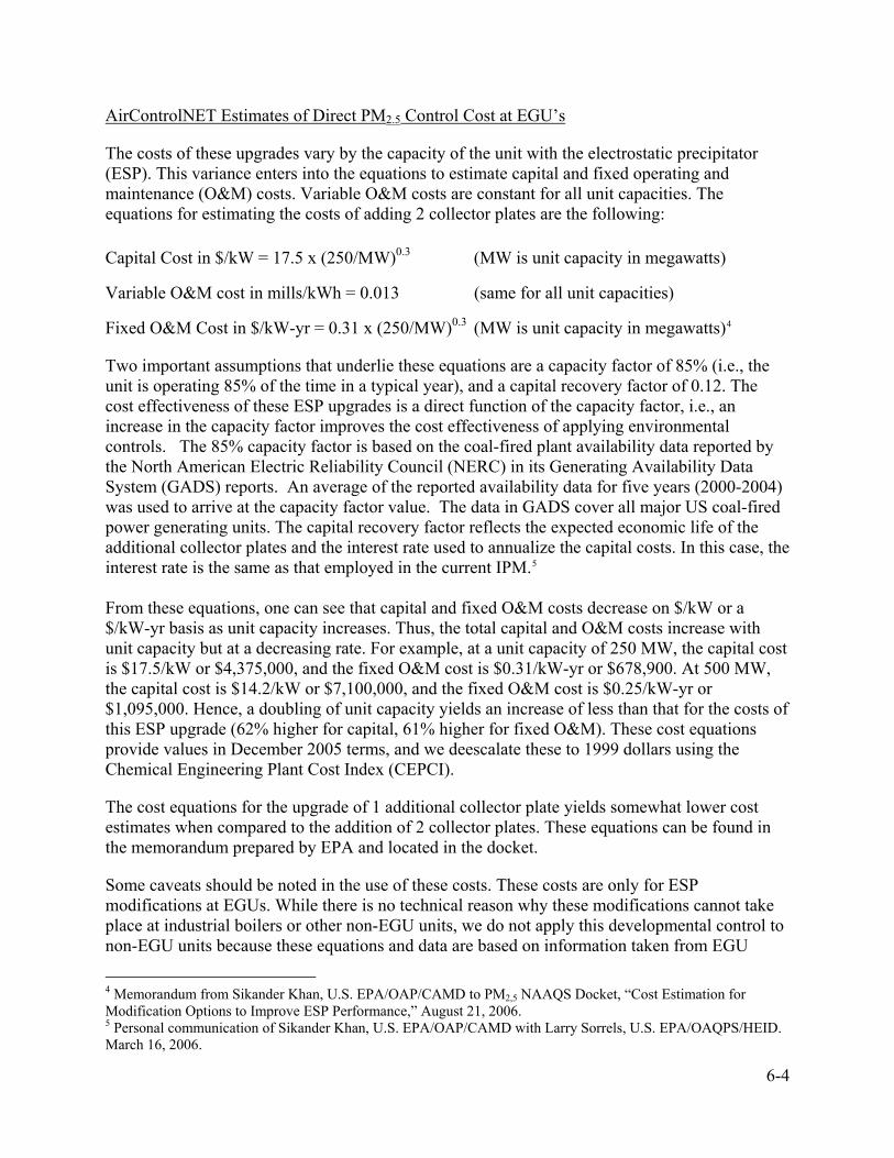
AirControlNET Estimates of Direct PM2.5 Control Cost at EGU’s
The costs of these upgrades vary by the capacity of the unit with the electrostatic precipitator (ESP). This variance enters into the equations to estimate capital and fixed operating and maintenance (O&M) costs. Variable O&M costs are constant for all unit capacities. The equations for estimating the costs of adding 2 collector plates are the following:
Capital Cost in $/kW = 17.5 x (250/MW)0.3 (MW is unit capacity in megawatts)
Variable O&M cost in mills/kWh = 0.013 (same for all unit capacities)
Fixed O&M Cost in $/kW-yr = 0.31 x (250/MW)0.3 (MW is unit capacity in megawatts)4
Two important assumptions that underlie these equations are a capacity factor of 85% (i.e., the unit is operating 85% of the time in a typical year), and a capital recovery factor of 0.12. The cost effectiveness of these ESP upgrades is a direct function of the capacity factor, i.e., an increase in the capacity factor improves the cost effectiveness of applying environmental controls. The 85% capacity factor is based on the coal-fired plant availability data reported by the North American Electric Reliability Council (NERC) in its Generating Availability Data System (GADS) reports. An average of the reported availability data for five years (2000-2004) was used to arrive at the capacity factor value. The data in GADS cover all major US coal-fired power generating units. The capital recovery factor reflects the expected economic life of the additional collector plates and the interest rate used to annualize the capital costs. In this case, the interest rate is the same as that employed in the current IPM.5
From these equations, one can see that capital and fixed O&M costs decrease on $/kW or a $/kW-yr basis as unit capacity increases. Thus, the total capital and O&M costs increase with unit capacity but at a decreasing rate. For example, at a unit capacity of 250 MW, the capital cost is $17.5/kW or $4,375,000, and the fixed O&M cost is $0.31/kW-yr or $678,900. At 500 MW, the capital cost is $14.2/kW or $7,100,000, and the fixed O&M cost is $0.25/kW-yr or $1,095,000. Hence, a doubling of unit capacity yields an increase of less than that for the costs of this ESP upgrade (62% higher for capital, 61% higher for fixed O&M). These cost equations provide values in December 2005 terms, and we deescalate these to 1999 dollars using the Chemical Engineering Plant Cost Index (CEPCI).
The cost equations for the upgrade of 1 additional collector plate yields somewhat lower cost estimates when compared to the addition of 2 collector plates. These equations can be found in the memorandum prepared by EPA and located in the docket.
Some caveats should be noted in the use of these costs. These costs are only for ESP modifications at EGUs. While there is no technical reason why these modifications cannot take place at industrial boilers or other non-EGU units, we do not apply this developmental control to non-EGU units because these equations and data are based on information taken from EGU
4 Memorandum from Sikander Khan, U.S. EPA/OAP/CAMD to PM2,5 NAAQS Docket, “Cost Estimation for Modification Options to Improve ESP Performance,” August 21, 2006. 5 Personal communication of Sikander Khan, U.S. EPA/OAP/CAMD with Larry Sorrels, U.S. EPA/OAQPS/HEID. March 16, 2006.
6-4

operations and hence may not be appropriate for application to non-EGU units. In addition, these costs are preliminary in nature and there is need for more detailed results to confirm their accuracy.
6.1.3 Mobile Sources
Cost information for mobile source controls was taken from studies conducted by EPA for previous rulemakings and studies conducted for development of voluntary and local measures that could be used by state or local programs to assist in improving air quality. These studies are mentioned further in section 6.2.3. Links to specific references are available at the website for EPA's Office of Transportation and Air Quality, www.epa.gov/otaq.
6.2 Cost by Sector
In this section, we provide engineering cost estimates of the control strategies identified in Chapter 3 that include control technologies on non-EGU stationary sources, area sources, electric generating units, and mobile sources. Engineering costs generally refer to the capital equipment expense, the site preparation costs for the application, and annual operating and maintenance costs. These costs serve as input to the economic impact analysis presented in Section 6, which produces an estimate of the quantifiable social cost of the regulatory option analyzed in this RIA. The total annualized cost of each control scenario is provided in Table 6-1 and reflects the engineering costs across sectors that are annualized at an interest rate of 7 percent; we also provide a summary estimate of engineering cost at a 3 percent discount rate. Total annualized cost of the revised standard, incremental to the current standard, is approximately $5 billion. Of this incremental cost of $5 billion, approximately $4.3 billion in costs are attributable to the extrapolated full attainment costs for California and Salt Lake City, which are speculative (see Section 6.4 below for a full discussion of the extrapolation methodology). To provide some context of this cost to society, this cost estimate is roughly equivalent to $35 per household per year in the U.S. The total annualized cost of the more stringent alternative for the annual standard, incremental to the current standard is approximately $7 billion (or $1.9 billion in additional costs over and above the revised standard of 15/35), which equates to approximately $50 per household in the U.S. Of this incremental cost of $7 billion, about $4.3 billion are attributable to the extrapolated full attainment costs for California and Salt Lake City, which are speculative. The economic impact analysis also provides a more in-depth evaluation of how the engineering costs will impact society through a distributional analysis of changes in price and production levels in affected industries, and who will bear the burden of the regulatory costs (consumers or suppliers).
Note that the cost estimates provided in table 6-1 are comprised of modeled, supplemental and extrapolated costs. Cost estimates for EGU’s, mobile sources and other industrial sources are modeled engineering cost. The incremental cost of residual non-attainment is comprised of both supplemental and extrapolated control costs. In the subsections that follow we describe how we derived each of these control cost categories.
6-5

Tables 6-2 and 6-3 display total annualized cost of “modeled” controls by State (at a 7% interest rate) for non-EGU stationary and area sources, respectively. Details of the costs for each sector of control are provided in Sections 6.2.1 through 6.2.3.
6-6
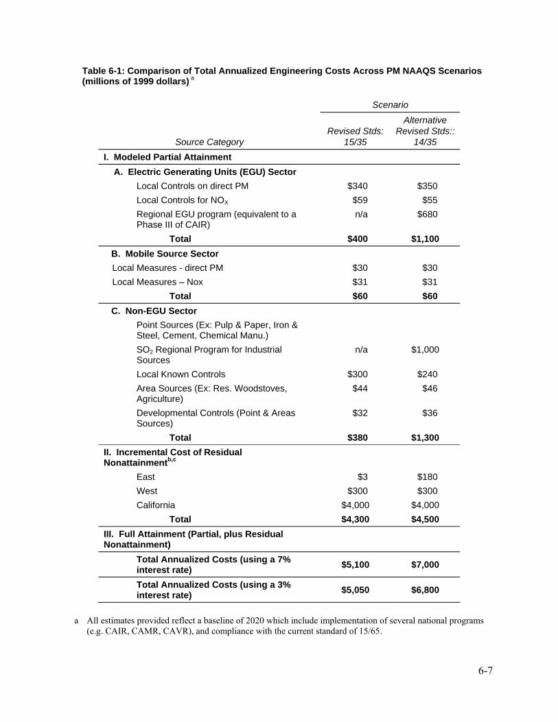
Table 6-1: Comparison of Total Annualized Engineering Costs Across PM NAAQS Scenarios (millions of 1999 dollars) a
Scenario
Source Category Revised Stds:
15/35
Alternative Revised Stds::
14/35 I. Modeled Partial Attainment A. Electric Generating Units (EGU) Sector
Local Controls on direct PM $340 $350 Local Controls for NOX $59 $55 Regional EGU program (equivalent to a Phase III of CAIR)
n/a $680
Total $400 $1,100 B. Mobile Source Sector
Local Measures - direct PM $30 $30 Local Measures – Nox $31 $31 Total $60 $60
C. Non-EGU Sector Point Sources (Ex: Pulp & Paper, Iron & Steel, Cement, Chemical Manu.)
SO2 Regional Program for Industrial Sources
n/a $1,000
Local Known Controls $300 $240 Area Sources (Ex: Res. Woodstoves, Agriculture)
$44 $46
Developmental Controls (Point & Areas Sources)
$32 $36
Total $380 $1,300 II. Incremental Cost of Residual Nonattainmentb,c
East $3 $180 West $300 $300 California $4,000 $4,000
Total $4,300 $4,500 III. Full Attainment (Partial, plus Residual Nonattainment)
Total Annualized Costs (using a 7% interest rate) $5,100 $7,000
Total Annualized Costs (using a 3% interest rate) $5,050 $6,800
a All estimates provided reflect a baseline of 2020 which include implementation of several national programs
(e.g. CAIR, CAMR, CAVR), and compliance with the current standard of 15/65.
6-7
6-8
b Upon review of emissions and air quality results of the control strategies applied in this RIA, some areas were indicated with residual nonattainment (requiring additional reductions to meet the standard) as a result of our initial selection of controls. The incremental costs of residual nonattainment reflect supplemental controls and extrapolated costs of additional control measures that would be necessary to bring areas with residual nonattainment into compliance. Chapter 4 provides details of the assessment. Numbers may not sum due to rounding.
c The incremental cost of residual non-attainment for the West and California are extrapolated. The methodology used to derive these estimates is described in Chapter 6. These estimates are derived using a 7 percent discount rate.
6.2.1 Non-EGU Stationary and Area Sources
In Table 6-2 and 6-3 below, we present the total annualized cost to each State for the proposed standard and the more stringent alternative. The costs reflected in this table represent annualized costs of the modeled attainment strategies (including local known controls on point and area sources as well as developmental controls) selected for analysis of the two regulatory options. We also provide some observations about the cost estimates that provide some insight into the control strategies selected. Readers interested in reviewing each of the emission controls we applied can consult the Emission Controls Technical Support Document, located in the docket.

Table 6-2: Total Annualized Costs of Modeled Attainment Strategies Applied to Non-EGU (Point) Stationary Sources: Costs by State and Pollutant Category* (millions of 1999$)
State Pollutant
Total Incremental Annualized Cost
of 15/35
Total Incremental Annualized Cost
of 14/35 Observations Alabama SO2 $0 $36 Total $0 $36
Costs reflect controls of the SO2 regional program considered for the 14/35 scenario. Alabama is not projected to be in nonattainment for the revised daily standard once the area complies with the current standard of 15/65
California NOx $0 $1 PM2.5 $3 $3 Total $3 $4
Incremental control for the annual 14 std. and the daily 35 std reflect additional counties that attained 15/65 but do not attain the new daily standard and the more stringent alternative std. analyzed
Georgia SO2 $0 $140 Total $0 $140
Costs reflect controls of the SO2 regional program considered for the 14/35 scenario
Idaho NOx $2 $2 PM2.5 $3 $3 Total $5 $5
Costs reflect controls selected to meet the daily standard only
Illinois SO2 $0 $140 Total $0 $140
Illinois complies with the daily standard at 35 µg when it complies with the 15/65 current standard. Costs reflect controls selected to meet the current standard and the SO2 regional program considered for 14/35.
Indiana SO2 $0 $170 Total $0 $170
Indiana complies with the daily standard at 35 µg when it complies with the 15/65 current standard. Costs reflect controls selected for the SO2 regional program considered for 14/35.
Kentucky SO2 $0 $48 Total $0 $48
Kentucky complies with the daily standard at 35 µg when it complies with the 15/65 current standard. Costs reflect controls selected to meet the current standard and the SO2 regional program considered for 14/35.
* Costs presented in this table are rounded to the nearest million and are incremental to costs of meeting the current standard of 15/65.
6-9

Table 6-2: Total Annualized Costs of Modeled Attainment Strategies Applied to Non-EGU Stationary (Point) Sources: Costs by State and Pollutant Category (continued)* (millions of 1999$)
State Pollutant
Total Incremental Annualized Cost
of 15/35
Total Incremental Annualized Cost
of 14/35 Observations Michigan NOx $0 $44 PM2.5 $0 <$1 SO2 $0 $160 Total $0 $200
Michigan meets the daily standard. Costs reflect controls selected for the SO2 regional program considered for 14/35 and other point source controls.
Missouri SO2 $0 $110 Total $0 $110
Costs reflect the SO2 regional program only
Montana NOx $3 $3 PM2.5 $13 $13 Total $16 $16
Costs reflect controls to meet the daily standard only.
Ohio PM2.5 $2 <$1 SO2 $0 $160 Total $2 $160
Costs reflect controls to meet the current standard, the new daily standard at 35 µg, the regional SO2 program considered for the 14/35 scenario that reduced the number of controls needed from direct PM2.5 sources.
Oregon NOx $10 $10 PM2.5 $11 $11 Total $21 $21
Cost reflect controls to meet the daily standard only.
Pennsylvania PM2.5 $28 $28 SO2 $72 $49 Total $100 $76
Control strategies required non-EGU stationary controls in all three regulatory scenarios analyzed for both the daily and annual standards
Utah PM2.5 <$1 <$1 Total <$1 <$1
Cost reflect controls to meet the daily standard only.
Washington NOx $84 $77 PM2.5 $25 $25 Total $109 $100
Cost reflect controls to meet the daily standard only.
West Virginia PM2.5 $15 $15 SO2 $38 $0 Total $54 $15
Although West Virginia attains the scenarios analyzed, controls strategies identified areas that may contribute to nonattainment issues in other locations. This analysis assumes State authorities will coordinate to define control strategies that bring an area into attainment at the lowest social cost.
* Costs presented in this table are rounded to the nearest million and are incremental to costs of meeting the current standard of 15/65.
6-10

Table 6-2: Total Annualized Costs of Modeled Attainment Strategies Applied to Non-EGU Stationary (Point) Sources: Costs by State and Pollutant Category (continued)* (millions of 1999$)
State Pollutant
Total Incremental Annualized Cost
of 15/35
Total Incremental Annualized Cost
of 14/35 Observations
Total Annualized Costs for the Non-EGU point source sector (7% Discount Rate)
$310 $1,200
Total Annualized Costs for the Non-EGU point source sector (3% Discount Rate)
$290 $1,200
* Costs presented in this table are rounded to the nearest million and are incremental to costs of meeting the current standard of 15/65.
6-11
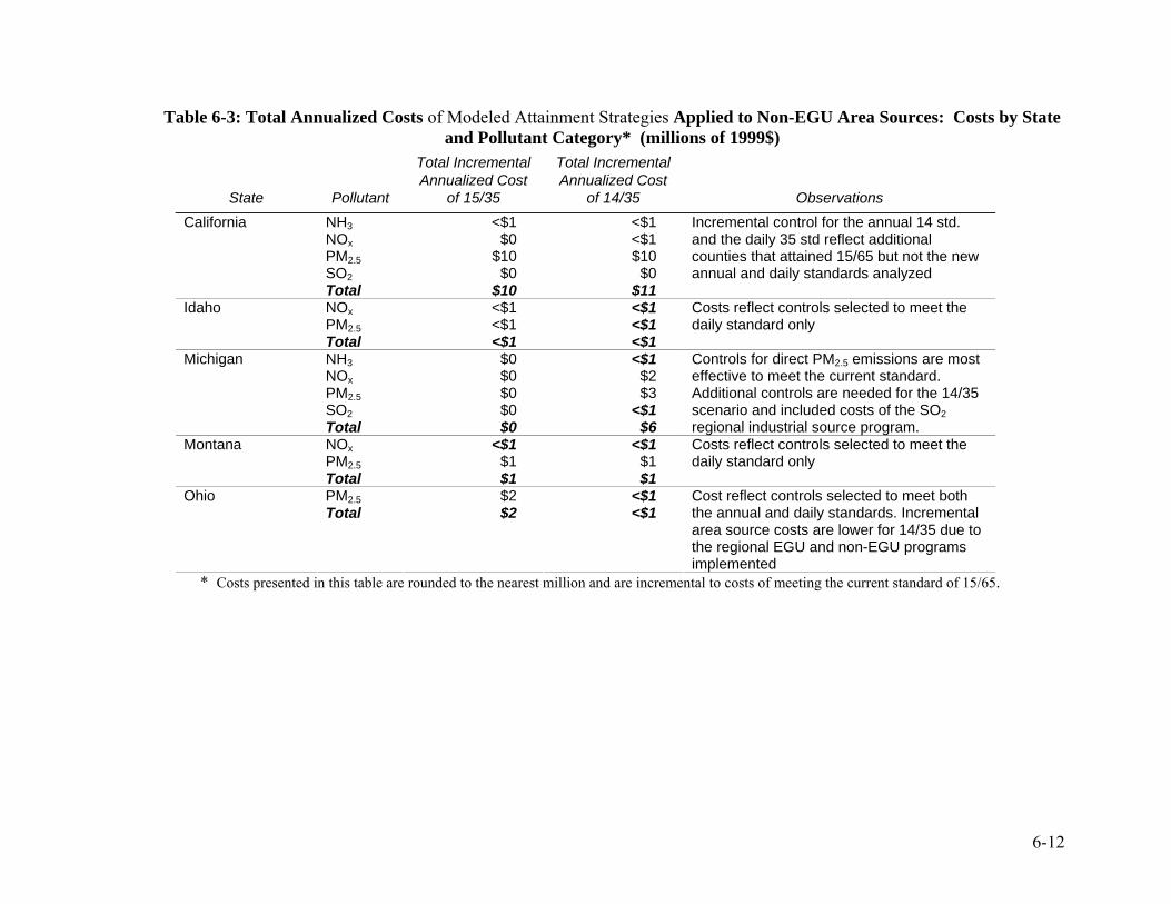
Table 6-3: Total Annualized Costs of Modeled Attainment Strategies Applied to Non-EGU Area Sources: Costs by State and Pollutant Category* (millions of 1999$)
State Pollutant
Total Incremental Annualized Cost
of 15/35
Total Incremental Annualized Cost
of 14/35 Observations California NH3 <$1 <$1 NOx $0 <$1 PM2.5 $10 $10 SO2 $0 $0 Total $10 $11
Incremental control for the annual 14 std. and the daily 35 std reflect additional counties that attained 15/65 but not the new annual and daily standards analyzed
Idaho NOx <$1 <$1 PM2.5 <$1 <$1 Total <$1 <$1
Costs reflect controls selected to meet the daily standard only
Michigan NH3 $0 <$1 NOx $0 $2 PM2.5 $0 $3 SO2 $0 <$1 Total $0 $6
Controls for direct PM2.5 emissions are most effective to meet the current standard. Additional controls are needed for the 14/35 scenario and included costs of the SO2 regional industrial source program.
Montana NOx <$1 <$1 PM2.5 $1 $1 Total $1 $1
Costs reflect controls selected to meet the daily standard only
Ohio PM2.5 $2 <$1 Total $2 <$1
Cost reflect controls selected to meet both the annual and daily standards. Incremental area source costs are lower for 14/35 due to the regional EGU and non-EGU programs implemented
* Costs presented in this table are rounded to the nearest million and are incremental to costs of meeting the current standard of 15/65.
6-12

6-13
Table 6-3: Total Annualized Costs of Modeled Attainment Strategies Applied to Non-EGU Area Sources: Costs by State and Pollutant Category (continued)* (millions of 1999$)
State Pollutant
Total Incremental Annualized Cost
of 15/35
Total Incremental Annualized Cost
of 14/35 Observations Oregon NH3 <$1 <$1 NOx <$1 <$1 PM2.5 $22 $22 SO2 <$1 <$1 Total $24 $24
Costs reflect controls selected to meet the daily standard only
Pennsylvania NH3 <$1 <$1 PM2.5 $17 $17 SO2 $4 $4 Total $22 $22
Costs reflect controls selected to meet the daily standard only. The more stringent annual standard of 14 µg is met through EGU and non-EGU point source controls.
Utah PM2.5 $3 $3 Total $3 $3
Costs reflect controls selected to meet the daily standard only
Washington NOx $1 $2 PM2.5 $6 $6 SO2 $1 $1 Total $9 $9
Costs reflect controls selected to meet the daily standard only
West Virginia PM2.5 <$1 <$1 SO2 <$1 <$1 Total <$1 <$1
Although West Virginia attains the scenarios analyzed, controls strategies identified areas that may contribute to nonattainment issues in other locations. This analysis assumes State authorities will coordinate to define control strategies that bring an area into attainment at the lowest social cost.
Total Annualized Cost for the Area Source Sector (7% Discount Rate)
$72 $77
Total Annualized Cost for the Area Source Sector (3% Discount Rate)
$71 $75
* Costs presented in this table are rounded to the nearest million and are incremental to costs of meeting the current standard of 15/65.

Draft—Not for Distribution
6.2.2 EGU Sources
Costs of Controls Outside the CAIR Region and Costs of Direct PM Controls Nationwide
In addition to the discussion of controls on EGU’s in Section 6.2.1, we also applied EGU controls to sources from the AirControlNET model. Controls selected are focused on those controls that are not considered part of the CAIR rule, such as direct PM2.5 control technologies, and in the Western U.S. controls for NOx emissions from these sources. The direct PM and NOx controls for EGU’s were selected only when this sector was identified as a cost-effective category for control strategies. In Table 6-4, incremental EGU controls for the selected standard are chosen only in a limited number of States, including: Ohio, Pennsylvania, Utah, and Washington, and are selected to help these areas attain a more stringent daily standard.
Table 6-4: Total Annualized Costs Applied to EGU Sources using AirControlNET*: Costs by State and Pollutant Category (millions of 1999$)
State Pollutant
Total Incremental Annualized Cost of
15/35
Total Incremental Annualized Cost of
14/35 Michigan PM2.5 $0 $36 Ohio PM2.5 $140 $110 Pennsylvania PM2.5 $190 $190 Utah NOx $55 $55 PM2.5 $13 $13 Total $68 $68 Washington PM2.5 $2.9 $2.9 West Virginia PM2.5 $0 $0 Wisconsin PM2.5 $0 $0 Total Annualized Cost for EGU sources from ACNet (7% Discount Rate)
$400 $410
Total Annualized Cost for EGU sources from ACNet (3% Discount Rate)
$360 $370
* Costs presented in this table are incremental to costs of meeting the current standard of 15/65.
Power Sector Impacts of Illustrative CAIR Extended Analysis As previously discussed, the power sector will achieve significant emission reductions under the Clean Air Interstate Rule (CAIR) over the next 10 to 15 years. When fully implemented, CAIR will reduce SO2 emissions in these States by over 70 percent and NOx emissions by over 60
6-14

Draft—Not for Distribution
percent from 2003 levels. These reductions will greatly improve air quality and will lessen the challenges that some areas face when solving nonattainment issues significantly. The analysis and projections in this section attempt to show the potential impacts of the Illustrative CAIR Extended approach to facilitate attainment of the more stringent alternative annual standard of 14 μ/m3 and daily standard of 35 μ/m3. Generally, the incremental impacts of the Illustrative CAIR Extended approach on the power sector are relatively modest. Projected Costs. EPA projects that the annual incremental costs of the Illustrative CAIR Extended approach are $0.51 billion in 2015 and $0.68 billion in 2020. The cost of electricity generation represents roughly one-third to one-half of total electricity costs, with transmission and distribution costs representing the remaining portion. The additional annual costs reflect additional retrofits (scrubbers), generation shifts, and the increased cost of allowances. Although the Illustrative CAIR Extended approach comes into effect in 2020 (with a third phase to CAIR), economic modeling indicates that the least-cost approach to complying involves changing banking patterns by reducing emissions prior to 2020. The additional reductions (and pollution controls) prior to 2020 result in additional costs to the power sector in 2015 as it complies in the most cost-effective manner. Figure 6-1. Incremental Annual Cost of CAIR and CAIR Extended for EGUs (billions $1999)
$6.17
$4.60
$0.51
$0.68
$0
$2
$4
$6
$8
2015 2020
CAIR Illustrative CAIR ExtendedSource: IPM
6-15

Draft—Not for Distribution
Figure 6-2. Marginal Cost of SO2 Allowances with CAIR and CAIR Extended for EGUs ($1999)
$1,137
$877
$990
$1,284
$0
$500
$1,000
$1,500
2015 2020
CAIR Illustrative CAIR ExtendedSource: IPM
Projected Generation Mix. Coal-fired generation and natural gas-fired generation are projected to remain relatively unchanged because of the phased-in nature of CAIR, which allows industry the appropriate amount of time to install the necessary pollution controls. The Illustrative CAIR Extended approach does not change the way the power sector produces electricity in any significant way, and changes in the electricity generation mix of the CAIR Extended approach, relative to CAIR, are negligible. Figure 6-3. Projected Generation Mix in 2010, 2015, and 2020 with CAIR and CAIR
Extended (TWh)
6-16
Draft—Not for Distribution
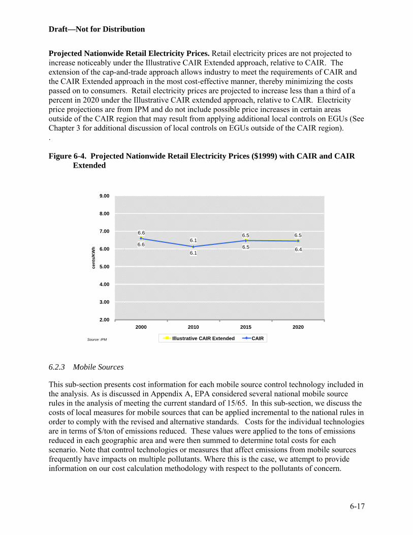
Projected Nationwide Retail Electricity Prices. Retail electricity prices are not projected to increase noticeably under the Illustrative CAIR Extended approach, relative to CAIR. The extension of the cap-and-trade approach allows industry to meet the requirements of CAIR and the CAIR Extended approach in the most cost-effective manner, thereby minimizing the costs passed on to consumers. Retail electricity prices are projected to increase less than a third of a percent in 2020 under the Illustrative CAIR extended approach, relative to CAIR. Electricity price projections are from IPM and do not include possible price increases in certain areas outside of the CAIR region that may result from applying additional local controls on EGUs (See Chapter 3 for additional discussion of local controls on EGUs outside of the CAIR region). . Figure 6-4. Projected Nationwide Retail Electricity Prices ($1999) with CAIR and CAIR
Extended
6.16.6
6.16.5
6.56.56.6
6.4
2.00
3.00
4.00
5.00
6.00
7.00
8.00
9.00
2000 2010 2015 2020
cent
s/K
Wh
Illustrative CAIR Extended CAIRSource: IPM
6.2.3 Mobile Sources
This sub-section presents cost information for each mobile source control technology included in the analysis. As is discussed in Appendix A, EPA considered several national mobile source rules in the analysis of meeting the current standard of 15/65. In this sub-section, we discuss the costs of local measures for mobile sources that can be applied incremental to the national rules in order to comply with the revised and alternative standards. Costs for the individual technologies are in terms of $/ton of emissions reduced. These values were applied to the tons of emissions reduced in each geographic area and were then summed to determine total costs for each scenario. Note that control technologies or measures that affect emissions from mobile sources frequently have impacts on multiple pollutants. Where this is the case, we attempt to provide information on our cost calculation methodology with respect to the pollutants of concern.
6-17

Draft—Not for Distribution
Note Regarding Mobile Source Air Toxics Rule The recent proposal to reduce mobile source air toxics (71 FR 15804, March 29, 2006) discusses data showing that direct PM2.5 emissions from gasoline vehicles are elevated at cold temperatures. The proposed vehicle hydrocarbon standards contained in the March 29, 2006 action would also reduce these elevated PM emissions. This RIA does not include the effects of this proposed rule because we do not currently have the data to model the impacts of elevated cold-temperature PM emissions across the entire in-use fleet. As a result, these cold-temperature emissions are not included in our baseline emission inventories, which may understate the baseline—and consequently projected—inventory of mobile source PM2.5
emissions. The final mobile source air toxics rule would thus reduce PM2.5 emissions, and improve air quality, by an amount not reflected in our analysis of these standards and may make compliance easier by reducing the need for some control strategies. EPA is currently analyzing these data from a large collaborative test program with industry, and our next emissions model (MOVES) will include cold temperature effects for PM. Geographical Scope of Mobile Source Controls It is important to clarify the sequence by which mobile source control measures were applied within the broader context of all control measures. In applying the cost information for the 15/35 and 14/35 scenarios, we first applied cost-effective local stationary source (point and area) controls. Next, due to time and analytical constraints, we applied local mobile source control measures only in areas where all available control measures were needed (southern California) and areas where a small additional amount of reductions would be needed to reach attainment (Chicago, Detroit, and the remaining areas in the West indicated by our air quality modeling as exceeding the standard). However, this does not imply that State and local authorities will sequence application of control measures in a similar fashion. State and local governments may have numerous reasons for employing mobile source control strategies before a set of measures that control point or area sources (for example, further point source controls would be less cost-effective than mobile measures, and/or an area’s stationary sources are already well-controlled). The following table lists the geographic areas to which mobile source control measures were applied.
6-18

Draft—Not for Distribution
Table 6-5: Geographic Areas to which Mobile Source Controls were Applied for 15/35 and 14/35
Geographic Area 15/35 & 14/35 Scenarios
National Rules All counties in the U.S. Southern California Chicago MSA Detroit MSA Missoula, MT MSA
Lincoln County, MT Shoshone County, ID Eugene-Springfield, OR MSA Klamath Falls, OR MSA Medford, OR MSA Logan, UT-ID MSA Salt Lake City, UT MSA Seattle-Bellevue-Everett, WA MSA
Local Measures
Tacoma, WA MSA More information on each of the rules and control measures can be found in Chapter 3, as well. In the table below, incremental mobile source controls for the selected standard are presented for the eastern U.S. (east of the Mississippi), western U.S. (except California), and California.
Table 6-6: Total Incremental Annualized Costs Applied to Mobile Sources (millions of 1999$)a
Geographic Area Pollutant
Total Incremental Annualized Cost of
15/35
Total Incremental Annualized Cost of
14/35 Eastern U.S. - Local Measures PM2.5 $7.4 $7.4 NOx $9.2 $9.2 Total $17 $17 Western U.S. (except CA) - Local Measures PM2.5 $7.6 $7.6 NOx $8.8 $8.8 Total $16 $16 California - Local Measures PM2.5 $15 $15 NOx $13 $13 Total $28 $28 Total Incremental Annualized Cost for Mobile Sources
$60 $60
a Estimates rounded to two significant figures for clarity of presentation
6-19
Draft—Not for Distribution
Emerging Mobile Source Technologies The control strategies employed in our mobile source analysis consist of, for the most part, regulations, tools, and programs that are based on well-understood pollution control technologies and techniques. Technologies to retrofit diesel engines, to take one example, are fairly well-established and are in use in communities around the country today, though further technological advances may result in increased efficiencies and lower costs. Our analysis did not incorporate what might be termed emerging or developmental mobile source control measures, although the history of control measures leads us to anticipate the emergence of new techniques and technologies that will lower emissions of PM2.5 and its precursors from mobile sources. For example, research is currently underway to develop even more efficient engine designs and emission control systems both for onroad vehicles and nonroad vehicles, engines, and equipment. Research topics include improving current technologies (e.g., particulate traps, highly efficient combustion techniques); possibly using on-road emission control technologies in nonroad vehicles, engines, and equipment; and various forms of other “clean” automotive technologies.6 This latter category includes a broad set of vehicle and fuel trends that are likely to have a substantial impact on the transportation sector, but for which data on costs and abatement efficiencies is either too scarce or simply unavailable, and therefore not suitable for inclusion in this analysis. Examples of technologies and other trends that were not analyzed as potential control measures include the following:
• Increased penetration of ethanol into the fuels market (either E10 or E85). Research relating to the net impacts on air emissions of ethanol use is ongoing.
• Research into other alternative, and possibly “cleaner,” fuels. • Advances in various forms of hybrid engine technologies. • Development of hydrogen fuel cell vehicles (H2FCVs) (and the concomitant hydrogen
supply infrastructure). • Congestion pricing systems (e.g., peak-period fees).
Estimated Costs of Local Measures Diesel Retrofits and Vehicle Replacement - For purposes of modeling, we divided the retrofit measure into two categories: the 1st 50% of retrofit potential (low end) and the 2nd 50% of retrofit potential (high end) to provide modeling and analytical flexibility with how such measures are applied. For example, such a division would help when applying retrofit measures to a nonattainment area in which only 50% of retrofit potential is adequate to achieve attainment. We categorize the low end as the most cost-effective retrofits since, ideally, states and local governments would first retrofit the most cost-effective fleets in terms of expected emissions reduction (based on vehicle miles traveled or VMT, expected life, model year, engine type, etc.) and cost of retrofit (based on technology and installation costs).
6More information can be found on EPA’s website, http://www.epa.gov/otaq/technology/index.htm#rel-links.
6-20
Draft—Not for Distribution
The cost-effectiveness ($/ton of PM) estimates for retrofits are based on EPA’s recent study of DOC and catalyzed DPF (CDPF) retrofits for school buses as well as class 6, 7, and 8b trucks; and just DOC retrofits for 250 hp bulldozers (the “C-E study”). The C-E study is available at http://www.epa.gov/cleandiesel/documents/420s06002.pdf. For purposes of the RIA, we believe this study is the best source of information since it is based on the most current data available. However, the C-E study was intentionally narrow in scope, and in using its data for an analysis as comprehensive as the RIA, raises a number of limitations that affect the data’s applicability. For example:
• The C-E study does not address several categories of engines analyzed in the retrofit measure for the RIA (e.g. Class 5 trucks, most nonroad engines).
• The C-E study does not estimate cost-effectiveness for repower or replacement, which are both included in the retrofit measure for the RIA.
• The C-E study is based on 2007 costs for technologies and emissions data for fleets. VMT, technology costs, and other variables will be different in 2015 and 2020.
• For highway engines, the C-E study is based on emission factors from recent testing which are higher than emissions factors found in MOBILE 6.2. EPA used the MOBILE 6.2 model to develop the inventory for the RIA and to analyze emissions reduction potential from retrofits. EPA will integrate the recent highway vehicle testing data into the next highway emissions model, MOVES. In the meantime, states and local governments will continue to use MOBILE 6.2 to estimate highway vehicle emissions for SIP and transportation conformity purposes.
For estimating the more cost-effective highway vehicle retrofits, we averaged the low end of the cost-effectiveness range of both measures (DOC and CDPF) for all three groups of highway vehicles in the C-E study (school buses, class 6 & 7 trucks, and class 8b trucks). For estimating the less cost-effective highway retrofits, we used the average of the range of cost-effectiveness of both measures and all three groups of vehicles. We used the average, rather than the high end of the cost-effectiveness range, because we believe that technology and installation costs are likely to decrease by 2015 and 2020. For the estimate of the cost-effectiveness of the low end potential of nonroad engine retrofits, we used the low end of the cost-effectiveness range for DOC retrofits of 250 hp bulldozers. For the estimate of the cost-effectiveness of the high end potential of nonroad engine retrofits, we used the average of the range of cost-effectiveness for DOC retrofits of 250 hp bulldozers. Again, we used the average, rather than the high end of the cost-effectiveness range, because we believe that technology and installation costs are likely to decrease by 2015 and 2020. The results are presented in Table 6-7 below:
6-21

Draft—Not for Distribution
Table 6-7. Cost Effectiveness for Diesel Retrofit Scenarios Summary of Cost-Effectiveness for Various Diesel PM Retrofit Scenarios (April 2006 EPA Study) $/ton PM Measure Min Max Average School Bus DOC $12,000 $49,100 $30,550 CDPF $12,400 $50,500 $31,450 Class 6&7 Truck DOC $27,600 $67,900 $47,750 CDPF $28,400 $69,900 $49,150 Class 8b Truck DOC $11,100 $40,600 $25,850 CDPF $12,100 $44,100 $28,100 250 hp Bulldozer DOC $18,100 $49,700 $33,900 Application to PM NAAQS RIA Package of Retrofit Measures (DOC, DPF, Repower, Replace) $/ton PM Highway (low end) $17,267 Highway (high end) $35,475 Nonroad (low end) $18,100 Nonroad (high end) $33,900
Note that these $/ton PM estimates are applied across the board for all types of retrofit measures (DOCs, CDPFs, repower, replacement) and highway vehicle and nonroad engine types. The overall cost-effectiveness of this measure is estimated to be:
• Highway 1st 50% - $17,267/ton PM • Highway 2nd 50% - $35,475/ton PM • Nonroad 1st 50% - $18,100/ton PM • Nonroad 2nd 50% - $33,900/ton PM
Eliminating Long Duration Truck Idling - For purposes of this RIA, we identified this measure as a no cost strategy: that is to say, at $0/ton PM. Both truck stop and terminal electrifications and mobile idle reduction technologies have upfront capital costs, but for the most part these costs can be fully recovered by fuel savings. The examples below illustrate the potential rate of return on investments in idle reduction strategies. Truck Stop and Terminal Electrifications (TSEs) The average price of TSE technology is $11,500 per parking space. The average service life of this technology is 15 years. Truck engines at idle consume approximately 1 gallon per hour of idle. Current TSE projects are operating in environments where trucks are idling, on average, for 8 hours per day per space for 365 days per year (or about 2,920 hours per year). Since TSE technology can completely eliminate long duration idling at truck spaces (i.e. a 100% fuel savings), this translates into 2,920 gallons of fuel saved per year per space. At current diesel prices ($2.90/gallon), this fuel savings translates into $8,468. Therefore, an $11,500 capital investment should be recovered within about 17 months. In this scenario, TSE investments offer over a 70% annual rate of return over the life of the technology.
6-22

Draft—Not for Distribution
While it is technically feasible to electrify all parking spaces that support long duration idling trucks, we should note that TSE technology is generally deployed at a minimum of 25-50 parking spaces per location to maximize economies of scale. The financial attractiveness of installing TSE technology will depend on the demonstrated truck idling behavior – the greater the rates of idling, the greater the potential emissions reductions and associated fuel and cost savings.
Mobile Idle Reduction Technologies (MIRTs) The price of MIRT technologies ranges from $1,000-$10,000. The most popular of these technologies is the auxiliary power unit (APU) because it provides air conditioning, heat, and electrical power to operate appliances. The average price of an APU is $7,000. The average service life of an APU is 10 years. An APU consumes two-tenths of a gallon per hour, so the net fuel savings is 0.80 gallons per hour. EPA estimates that trucks idle for 7 hours per rest period, on average, and about 300 days per year (or 2,100 hours per year). Since idling trucks consume 1 gallon of fuel per hour of idle, APUs can reduce fuel consumption for truck drivers/owners by approximately 1,680 gallons per year. At current diesel prices ($2.90/gallon), truck drivers/owners would save $4,872 on fuel if they used an APU. Therefore, a $7,000 capital investment should be recovered within about 18 months. In this scenario, APU investments offer almost a 70% annual rate of return over the life of the technology. Intermodal Transport - We believe that a 1% shift is viable and could occur at a low or no cost, since rail is likely to be less expensive than truck transport due primarily to lower fuel costs. For purposes of economic analysis, we identified this measure as a no cost strategy ($0/ton PM). A certain level of intermodal shifting may require new investments in rail infrastructure, but these costs should be fully recovered over time by the fuel and other transport cost savings. We did not have adequate data to conduct a more detailed cost analysis. Our understanding of costs is based on anecdotal evidence and confidential business information from partners in EPA’s SmartWay Transport Partnership program. There will be a great deal of variability in the financial attractiveness of transitioning to intermodal transport versus truck-only transport based on the capacity of current rail infrastructure; willingness of rail and truck companies to cooperate; the rail industry’s ability to make capital investments; and local government support for accommodating additional rail lines, rail facilities, and rail operation flexibility. Best Workplaces for Commuters (BWC) - We used the Transportation Research Board’s (TRB) cost-effectiveness analysis of Congestion Mitigation and Air Quality Improvement Program (CMAQ) projects to estimate the cost-effectiveness of this measure.7 TRB conducted an extensive literature review and then synthesized the data to develop comparable estimates of cost-effectiveness of a wide range of CMAQ-funded measures. We took the average of the median cost-effectiveness of a sampling of CMAQ-funded measures and then applied this number to the overarching BWC measure. The CMAQ-funded measures we selected were:
7 Transportation Research Board, National Research Council, 2002. The Congestion Mitigation and Air Quality Improvement Program: assessing 10 years of experience, Committee for the Evaluation of the Congestion Mitigation and Air Quality Improvement Program.
6-23
Draft—Not for Distribution
• regional rideshares • vanpool programs • park-and-ride lots • regional transportation demand management • employer trip reduction programs
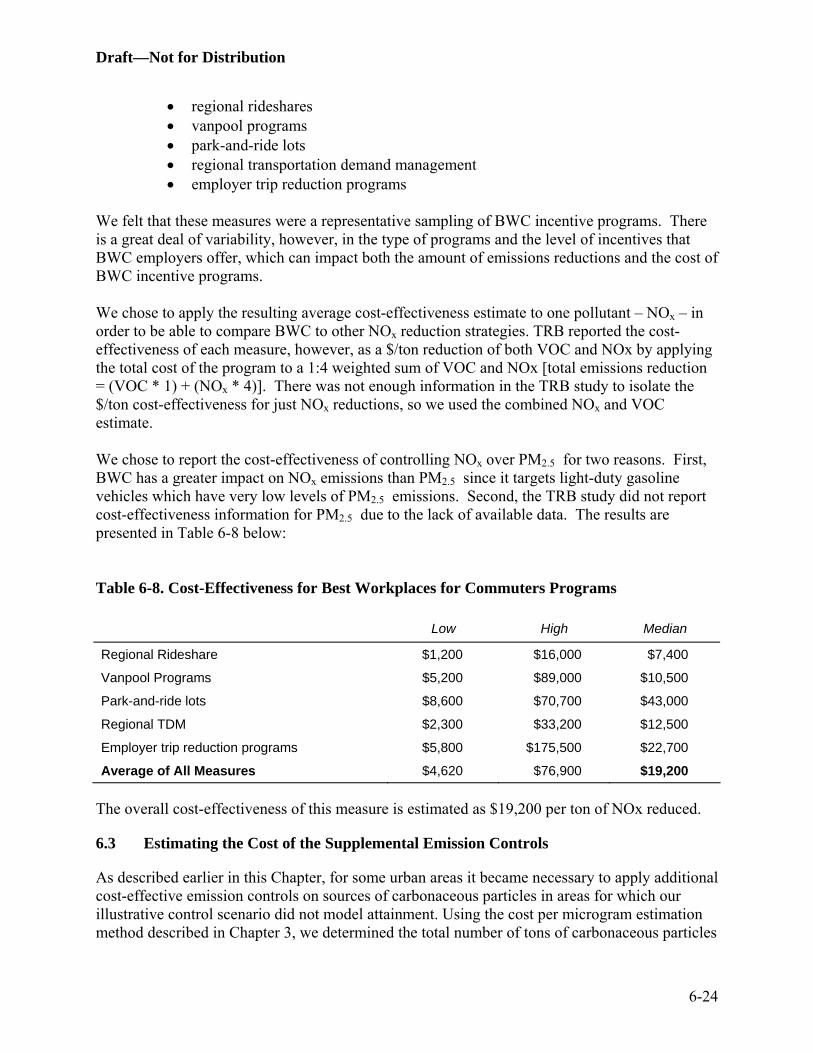
We felt that these measures were a representative sampling of BWC incentive programs. There is a great deal of variability, however, in the type of programs and the level of incentives that BWC employers offer, which can impact both the amount of emissions reductions and the cost of BWC incentive programs. We chose to apply the resulting average cost-effectiveness estimate to one pollutant – NOx – in order to be able to compare BWC to other NOx reduction strategies. TRB reported the cost-effectiveness of each measure, however, as a $/ton reduction of both VOC and NOx by applying the total cost of the program to a 1:4 weighted sum of VOC and NOx [total emissions reduction = (VOC * 1) + (NOx * 4)]. There was not enough information in the TRB study to isolate the $/ton cost-effectiveness for just NOx reductions, so we used the combined NOx and VOC estimate. We chose to report the cost-effectiveness of controlling NOx over PM2.5 for two reasons. First, BWC has a greater impact on NOx emissions than PM2.5 since it targets light-duty gasoline vehicles which have very low levels of PM2.5 emissions. Second, the TRB study did not report cost-effectiveness information for PM2.5 due to the lack of available data. The results are presented in Table 6-8 below: Table 6-8. Cost-Effectiveness for Best Workplaces for Commuters Programs
Low High Median
Regional Rideshare $1,200 $16,000 $7,400
Vanpool Programs $5,200 $89,000 $10,500
Park-and-ride lots $8,600 $70,700 $43,000
Regional TDM $2,300 $33,200 $12,500
Employer trip reduction programs $5,800 $175,500 $22,700
Average of All Measures $4,620 $76,900 $19,200
The overall cost-effectiveness of this measure is estimated as $19,200 per ton of NOx reduced.
6.3 Estimating the Cost of the Supplemental Emission Controls
As described earlier in this Chapter, for some urban areas it became necessary to apply additional cost-effective emission controls on sources of carbonaceous particles in areas for which our illustrative control scenario did not model attainment. Using the cost per microgram estimation method described in Chapter 3, we determined the total number of tons of carbonaceous particles
6-24

Draft—Not for Distribution
that would be necessary to reduce to simulate attainment with the revised or more stringent alternative standards. If additional cost-effective carbonaceous particle controls were available, we applied these controls to achieve a reduction in the estimated tonnage. Table 6-9 below summarizes the projected non-attainment areas to which we applied these controls as well as the total tons abated and the total cost.8
Table 6-9. Supplemental Emission Controls Applied on Sources of Carbonaceous Particles
PM2.5 Standard and Urban Area Tons Abated Total Cost (Million 1999$) 15/35
Cleveland 933 $3 14/35
Birmingham 3,600 $40 Chicago 3,490 $120
6.4 Estimating the Attainment Cost for California and Salt Lake City
As described in Chapter 3, California and Salt Lake City posed especially challenging attainment problems due to a confluence of data limitations and the magnitude of their non-attainment problem. Because we were unable to simulate full attainment using existing or supplemental emission controls, estimating the cost of attaining the residual non-attainment air quality increment required an alternative approach. Below we outline our cost estimation methodology and cost estimates for California and Salt Lake City.
Estimating the Attainment Cost for California
The magnitude of the projected non-attainment problem in California described in Chapter 3 necessitated using a cost-estimation methodology that differs from that used to derive cost for other areas of the country. Many sectors are already well controlled in California, and the additional “add-on” controls that we applied in this analysis did not result in significant emissions reductions. California is likely to rely much more on technological change and innovative control strategies (development and penetration of hydrogen fuel cell vehicles, for example). At the same time, because it is so much harder to predict the effectiveness and cost of new technologies or strategies, our final cost estimates showing California attainment are much more uncertain. As such, our analysis of California, and in particular our presentation of costs for the state, require a separate treatment in this RIA.
8 Note that supplemental control costs found in table 6-12 sum to $152M. This estimate is approximately $30M less than the engineering cost estimate we used when deriving economic costs (see Chapter 7). This discrepancy is due to the fact that we began the economic impact analysis prior to having finalized the supplemental control costs.
6-25
Draft—Not for Distribution
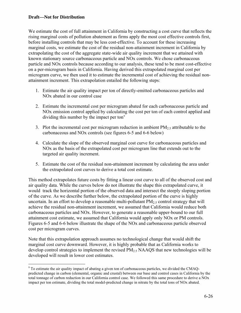
We estimate the cost of full attainment in California by constructing a cost curve that reflects the rising marginal costs of pollution abatement as firms apply the most cost effective controls first, before installing controls that may be less cost-effective. To account for these increasing marginal costs, we estimate the cost of the residual non-attainment increment in California by extrapolating the cost of the aggregate state-wide air quality increment that we attained with known stationary source carbonaceous particle and NOx controls. We chose carbonaceous particle and NOx controls because according to our analysis, these tend to be most cost-effective on a per-microgram basis in California. Having derived this extrapolated marginal cost per microgram curve, we then used it to estimate the incremental cost of achieving the residual non-attainment increment. This extrapolation entailed the following steps:
1. Estimate the air quality impact per ton of directly-emitted carbonaceous particles and NOx abated in our control case
2. Estimate the incremental cost per microgram abated for each carbonaceous particle and NOx emission control applied by calculating the cost per ton of each control applied and dividing this number by the impact per ton9
3. Plot the incremental cost per microgram reduction in ambient PM2.5 attributable to the carbonaceous and NOx controls (see figures 6-5 and 6-6 below)
4. Calculate the slope of the observed marginal cost curve for carbonaceous particles and NOx as the basis of the extrapolated cost per microgram line that extends out to the targeted air quality increment.
5. Estimate the cost of the residual non-attainment increment by calculating the area under the extrapolated cost curves to derive a total cost estimate.
This method extrapolates future costs by fitting a linear cost curve to all of the observed cost and air quality data. While the curves below do not illustrate the shape this extrapolated curve, it would track the horizontal portion of the observed data and intersect the steeply sloping portion of the curve. As we describe further below, the extrapolated portion of the curve is highly uncertain. In an effort to develop a reasonable multi-pollutant PM2.5 control strategy that will achieve the residual non-attainment increment, we assumed that California would reduce both carbonaceous particles and NOx. However, to generate a reasonable upper-bound to our full attainment cost estimate, we assumed that California would apply only NOx or PM controls. Figures 6-5 and 6-6 below illustrate the shape of the NOx and carbonaceous particle observed cost per microgram curves.
Note that this extrapolation approach assumes no technological change that would shift the marginal cost curve downward. However, it is highly probable that as California works to develop control strategies to implement the revised PM2.5 NAAQS that new technologies will be developed will result in lower cost estimates.
9 To estimate the air quality impact of abating a given ton of carbonaceous particles, we divided the CMAQ-predicted change in carbon (elemental, organic and crustal) between our base and control cases in California by the total tonnage of carbon reduction in our California control case. We followed this same procedure to derive a NOx impact per ton estimate, dividing the total model-predicted change in nitrate by the total tons of NOx abated.
6-26

Draft—Not for Distribution
Figure 6-5. Marginal cost per microgram of reducing PM2.5 through the application of NOx controls
Figure 6-6. Marginal cost per microgram of reducing PM2.5 through the application of carbonaceous particle controls
Both of these figures feature a steeply-sloping marginal cost curve, suggesting that the last remaining emission controls applied were relatively expensive and produced a small improvement in the annual design value. In these figures, each diamond or circle represents the
6-27
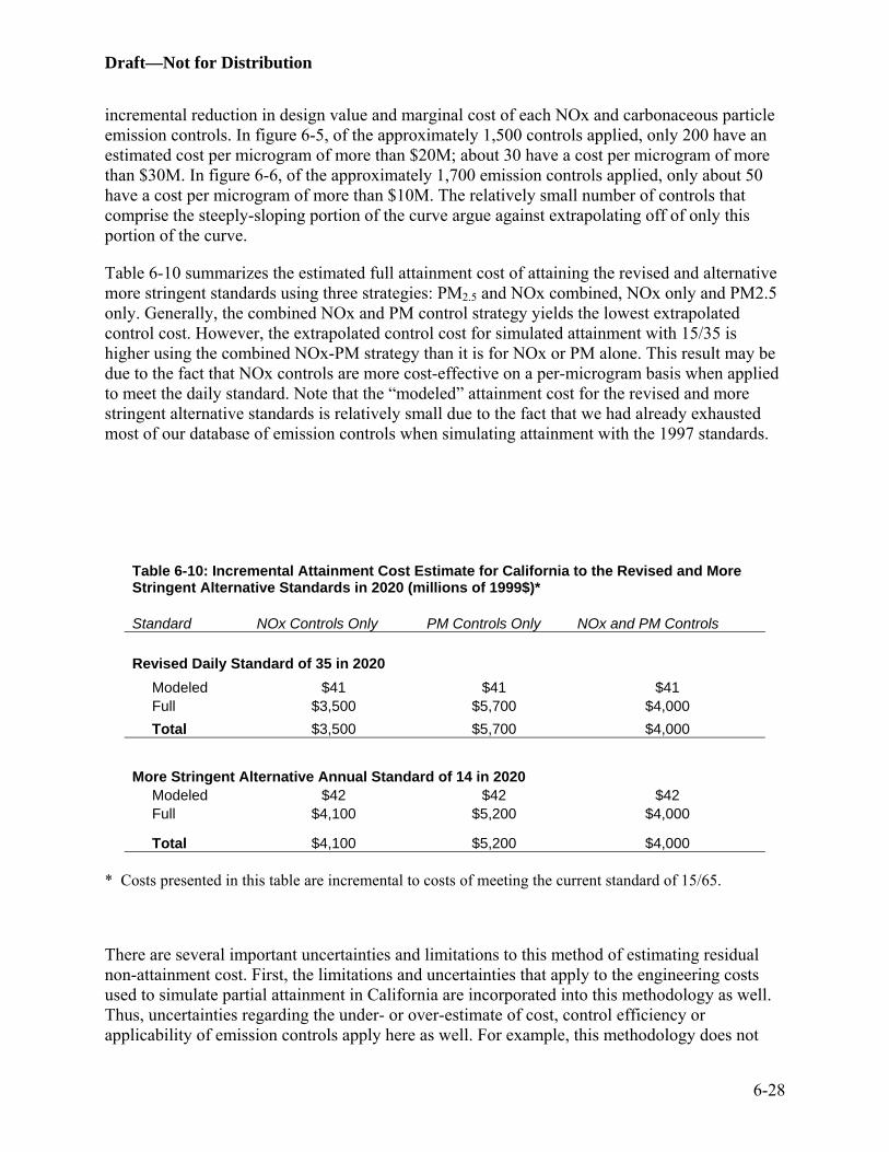
Draft—Not for Distribution
incremental reduction in design value and marginal cost of each NOx and carbonaceous particle emission controls. In figure 6-5, of the approximately 1,500 controls applied, only 200 have an estimated cost per microgram of more than $20M; about 30 have a cost per microgram of more than $30M. In figure 6-6, of the approximately 1,700 emission controls applied, only about 50 have a cost per microgram of more than $10M. The relatively small number of controls that comprise the steeply-sloping portion of the curve argue against extrapolating off of only this portion of the curve.
Table 6-10 summarizes the estimated full attainment cost of attaining the revised and alternative more stringent standards using three strategies: PM2.5 and NOx combined, NOx only and PM2.5 only. Generally, the combined NOx and PM control strategy yields the lowest extrapolated control cost. However, the extrapolated control cost for simulated attainment with 15/35 is higher using the combined NOx-PM strategy than it is for NOx or PM alone. This result may be due to the fact that NOx controls are more cost-effective on a per-microgram basis when applied to meet the daily standard. Note that the “modeled” attainment cost for the revised and more stringent alternative standards is relatively small due to the fact that we had already exhausted most of our database of emission controls when simulating attainment with the 1997 standards.
Table 6-10: Incremental Attainment Cost Estimate for California to the Revised and More Stringent Alternative Standards in 2020 (millions of 1999$)* Standard NOx Controls Only PM Controls Only NOx and PM Controls Revised Daily Standard of 35 in 2020 Modeled $41 $41 $41 Full $3,500 $5,700 $4,000 Total $3,500 $5,700 $4,000
More Stringent Alternative Annual Standard of 14 in 2020 Modeled $42 $42 $42 Full $4,100 $5,200 $4,000
Total $4,100 $5,200 $4,000
* Costs presented in this table are incremental to costs of meeting the current standard of 15/65.
There are several important uncertainties and limitations to this method of estimating residual non-attainment cost. First, the limitations and uncertainties that apply to the engineering costs used to simulate partial attainment in California are incorporated into this methodology as well. Thus, uncertainties regarding the under- or over-estimate of cost, control efficiency or applicability of emission controls apply here as well. For example, this methodology does not
6-28
Draft—Not for Distribution
attempt to capture the impacts learning-by-doing or technological innovation; both of these phenomena have historically resulted in downward/outward shifts of marginal cost curves or flattening of its slope. The result of our inability to capture such effects may be a conservative (high) cost estimate.
Second, estimated control cost is sensitive to assumptions regarding the appropriate portion of the observed cost curve off of which to estimate the slope. As described above, both the PM and NOx marginal cost curve bend steeply, suggesting that a relatively small number of high cost per-microgram controls are affecting the shape of the curve. This factor argues for using the slope of the full curve as the basis for extrapolation, rather than using only costs above or below the knee.
Third, there are uncertainties regarding the estimated air quality impact of a given ton of directly-emitted carbonaceous particles. To the extent that we have under- or over-estimated the average air quality impact across all violating California monitors of a given reduction in directly-emitted carbonaceous particles, these marginal cost estimates may be over- or under-estimated. Moreover, we assume that each marginal decrease in directly-emitted carbonaceous particles is close enough to influence the violating PM2.5 monitor.
Estimating the Attainment Cost in Salt Lake City
Data limitations prevented us from following the methodology that we employed to estimate California full attainment cost. Where we applied several hundred NOx and over one thousand carbonaceous particle emission controls across the state of California, we applied only a small handful of NOx emission controls and a few hundred carbonaceous particle controls in the Salt Lake urban area. Thus, we lacked the data points to derive a credible marginal cost per microgram curve.
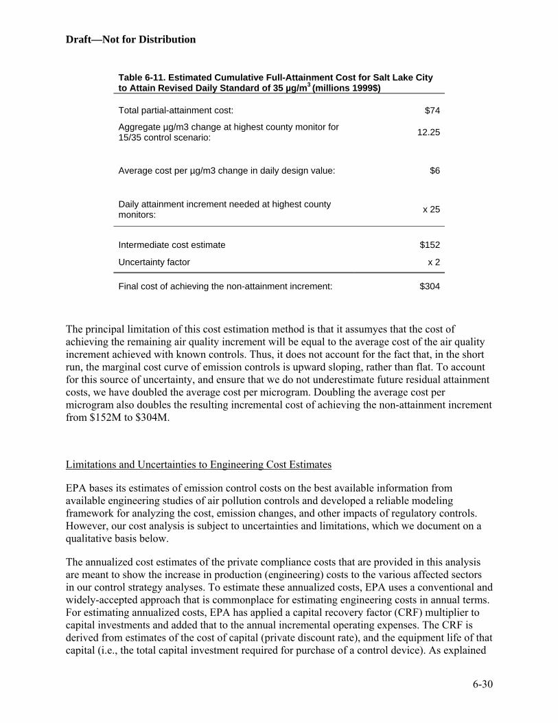
As an alternative, we estimated full attainment cost by multiplying the aggregate residual daily non-attainment increment by the average cost per microgram. Table 6-11 below summarizes these calculations.
6-29
Draft—Not for Distribution
Table 6-11. Estimated Cumulative Full-Attainment Cost for Salt Lake City to Attain Revised Daily Standard of 35 µg/m3 (millions 1999$) Total partial-attainment cost: $74
Aggregate µg/m3 change at highest county monitor for 15/35 control scenario: 12.25
Average cost per µg/m3 change in daily design value: $6
Daily attainment increment needed at highest county monitors: x 25
Intermediate cost estimate $152
Uncertainty factor x 2
Final cost of achieving the non-attainment increment: $304
The principal limitation of this cost estimation method is that it assumyes that the cost of achieving the remaining air quality increment will be equal to the average cost of the air quality increment achieved with known controls. Thus, it does not account for the fact that, in the short run, the marginal cost curve of emission controls is upward sloping, rather than flat. To account for this source of uncertainty, and ensure that we do not underestimate future residual attainment costs, we have doubled the average cost per microgram. Doubling the average cost per microgram also doubles the resulting incremental cost of achieving the non-attainment increment from $152M to $304M.
Limitations and Uncertainties to Engineering Cost Estimates
EPA bases its estimates of emission control costs on the best available information from available engineering studies of air pollution controls and developed a reliable modeling framework for analyzing the cost, emission changes, and other impacts of regulatory controls. However, our cost analysis is subject to uncertainties and limitations, which we document on a qualitative basis below.
The annualized cost estimates of the private compliance costs that are provided in this analysis are meant to show the increase in production (engineering) costs to the various affected sectors in our control strategy analyses. To estimate these annualized costs, EPA uses a conventional and widely-accepted approach that is commonplace for estimating engineering costs in annual terms. For estimating annualized costs, EPA has applied a capital recovery factor (CRF) multiplier to capital investments and added that to the annual incremental operating expenses. The CRF is derived from estimates of the cost of capital (private discount rate), and the equipment life of that capital (i.e., the total capital investment required for purchase of a control device). As explained
6-30

Draft—Not for Distribution
earlier in this RIA, we apply a 7 percent and three percent discount rate for annualizing the costs for non-EGU point and area sources over the equipment life where available for the control device. Information on the equipment life for different control devices can be found in the control measures documentation report for AirControlNET (EPA, 2006). The private compliance costs presented earlier are EPA’s best estimate of the direct private compliance costs for these illustrative control strategies.
The direct private compliance cost includes, but is not limited to, capital investments in pollution controls as an up front and an annualized costs, and operating and maintenance (or O&M) expenses. The methodology employed by EPA to estimate the costs of control can be found in the EPA Air Pollution Control Cost Manual (EPA, 2002). EPA believes that the cost assumptions used for non-EGU point and area sources and direct PM2.5 controls for EGUs reflect, as closely as possible, the best information available to the Agency today. The cost associated with monitoring emissions, reporting, and record keeping for affected sources is not included in these annualized cost estimates, but EPA believes these costs should be minor in comparison to the control costs based on the estimates prepared for the PM2.5 Implementation Rule Information Collection Request (ICR).
Furthermore, there are some unquantified costs that EPA wants identifies as limitations to its illustrative analyses. These costs include the costs of federal and State administration of the program, which we believe are less than the alternative of States developing approvable SIPs, securing EPA approval of those SIPs, and Federal/State enforcement. The Agency also did not consider transactional costs and/or effects on labor supply in these illustrative analyses.
From another vantage point, the illustrative analysis for non-EGU point and area source controls and direct PM2.5 controls for EGUs does not take into account the potential for advancements in the capabilities of pollution control technologies as well as reductions in their costs over time. In recognition of this factor, EPA’s mobile source program uses adjusted engineering cost estimates of pollution control equipment and installation costs to account for this fact and these are included in the mobile source costs presented in this RIA.10 We do not have sufficient information to adjust engineering cost estimates for non-EGU point and area source controls and direct PM2.5 controls for EGUs nor for other EGU controls at this time.
Also, as noted in Chapter 3, the costs estimated for non-EGU point and area source controls and mobile source controls are engineering costs only; they do not take into account the response of consumers to increases in product prices resulting from applications of these controls. Consumer responses related to application of these controls and all of the EGU controls, however, are estimated as part of the economic impact analyses generated by EMPAX and presented in Chapter 7 of this RIA. The direct engineering costs estimated in this RIA do not reflect the actual impact of these illustrative controls on consumers. Given some price elasticity of demand for products whose consumption is affected by the implementation of these illustrative controls, the actual impact to consumers will be less than that implied by the direct engineering controls. 10 See recent regulatory impact analysis for the Tier 2 Regulations for passenger vehicles (1999) and Heavy-Duty Diesel Vehicle Rules (2000). There is also evidence that scrubber costs will decrease in the future because of the learning_by_doing phenomenon, as more scrubbers are installed (see Manson, Nelson, and Neumann, 2002. “Assessing the Impact of Progress and Learning Curves on Clean Air Act Compliance Costs,” Industrial Economics Incorporated).
6-31

Draft—Not for Distribution
The greater the price elasticity of demand for a given affected product, the higher the impact on demand for that product by a consumer. See Chapter 7 of this RIA for more details.
Recent research suggests that the total social costs of a new regulation may be affected by interactions between the new regulation and pre-existing distortions in the economy, such as taxes. In particular, if cost increases due to a regulation are reflected in a general increase in the price level, the real wage received by workers may be reduced, leading to a small fall in the total amount of labor supplied. This “tax interaction effect” may result in an increase in deadweight loss in the labor market and an increase in total social costs. Although there is a good case for the existence of the tax interaction effect, recent research also argues for caution in making prior assumptions about its magnitude. Chapter 8 of EPA’s draft “Guidelines for Preparing Economic Analysis” discusses in detail the tax interaction effect in the context of environmental regulation. These economic analysis guidelines are still under review within EPA.
On balance, after consideration of various unquantified costs (and savings that are possible), EPA believes that the annual private compliance costs that we have estimated are more likely to overstate the future annual compliance costs that industry will incur, rather than understate those costs.
Technological Innovation, Learning-by-Doing, and Cost Estimates
We note that historically, compliance costs over long time periods have consistently been overestimated in regulatory analyses. Cost estimates frequently do not capture the effects of learning-by-doing or technological innovation and diffusion. The historical role of the CAA as a “technology-forcing” law, as well as a review of currently developing technologies, provides a sound basis for anticipating that technological progress will continue in response to new standards. It is difficult to predict technological improvements and their associated effects on cost because we have insufficient knowledge of which new technologies will be successful enough to have a meaningful impact on costs over the next ten to fifteen years—though history tells us such innovations will occur. This dynamic must be examined alongside observations regarding increasing marginal abatement costs.
6.5 Summary of Incremental Costs
Table 6-12 below summarizes the annualized costs of modeled control strategies that achieve partial attainment with the regulatory scenarios, as well as the supplemental and extrapolated engineering control costs (see Chapter 4 for a complete discussion of supplemental and extrapolated costs).
6-32

Draft—Not for Distribution
Table 6-12. Summary of Modeled Engineering, Supplemental and Extrapolated Engineering Attainment Costs (millions of 1999$)
Revised Standards: 15/35 Alternative More Stringent
Standards: 14/35
Cost estimate
3 Percent Discount Rate
7 Percent Discount Rate
3 Percent Discount Rate
7 Percent Discount Rate
Modeled Partial Attainment
$770 $840 $2,300 $2,500
Supplementala $3 $3 $170 $180
Extrapolatedb $4,300 $4,300 $4,300 $4,300
Total Annualized Cost of Full Attainment
$5,050 $5,100 $6,800 $7,000
a Upon review of emissions and air quality results of the control strategies applied in this RIA, some areas were indicated with residual nonattainment (requiring additional reductions to meet the standard) as a result of our initial selection of controls. The incremental costs of residual nonattainment reflect supplemental controls and extrapolated costs of additional control measures that would be necessary to bring areas with residual nonattainment into compliance. Chapter 4 provides details of the assessment. Numbers may not sum due to rounding.
b The incremental cost of residual non-attainment for the West and California are extrapolated. The methodology used to derive these estimates is described in Chapter 6. These estimates are derived using a 7 percent discount rate.
6.6 References
Manson, C.J., M.B. Nelson, and J.C. Neumann, 2002. “Assessing the Impact of Progress and Learning Curves on Clean Air Act Compliance Costs,” Industrial Economics Inc. July 12, 2002.
Pechan, 2006a. Memorandum from Frank Divita, E.H. Pechan and Associates, Inc. to Larry Sorrels, U.S. Environmental Protection Agency, “AirControlNET – Cost Equations and Default Information,” May 12, 2006.
Pechan, 2006b. Air ControlNET version 4.1, Control Measure Documentation Report. May 2006. Prepared for the U.S. Environmental Protection Agency (EPA). Office of Air Quality Planning and Standards.
U.S. Environmental Protection Agency (EPA). July 2002. EPA Air Pollution Control Cost Manual. Sixth Edition. EPA-452/B-02-001. Found on the Internet at http://www.epa.gov/ttn/catc/products.html#cccinfo.
6-33