Chapter 7 – Sampling Distributions of Estimates X X Xdinov/courses_students.dir/STAT13_Fall01/STAT13... · Chapter 7 – Sampling Distributions of Estimates 1. ... standard deviation

Stat 13, UCLA – Chapter 7 1

UCLA STAT 13 Statistical Methods Final Exam Review Chapter 7 – Sampling Distributions of Estimates

1. A random sample of size n is drawn from a population with mean, µ, and standard deviation, σ. Let

X be the sample mean.

(a) What is the: (i) mean of X ? (ii) standard deviation of X ?

(b) If we are sampling from a Normal distribution then X is exactly / approximately (circle one) Normally distributed.

(c) (i) If we are sampling from a non-Normal distribution then for large samples (ie, n is large)

X is exactly / approximately (circle one) Normally distributed.

(ii) The result in (i) is called the 2. A random sample of size n is drawn from a population in which a proportion p has a characteristic of

interest. Let P be the sample proportion.

(a) What is the: (i) mean of P ? (ii) standard deviation of P ?

(b) For large samples P is exactly / approximately (circle one) Normally distributed.

3. A __________________________________________ is a numerical characteristic of a population.

4. An ______________________________________ is a

quantity calculated from data in order to estimate an unknown .

5. Suppose that X1, X2, . . . , X16 is a random sample from a Normal distribution with mean of 50 and a

standard deviation of 10. Then the distribution of the sample mean 16

1621 XXXX +++=

K has

mean, Xµ , and standard deviation, Xσ , given by: (1) Xµ = 50, Xσ = 6.25

(2) Xµ = 50, Xσ = 0.625

(3) Xµ = 800, Xσ = 10

(4) Xµ = 50, Xσ = 2.5

(5) cannot be determined because n = 16 is too small for the central limit effect to take effect.

Stat 13, UCLA Final Exam – Chapter 7 2

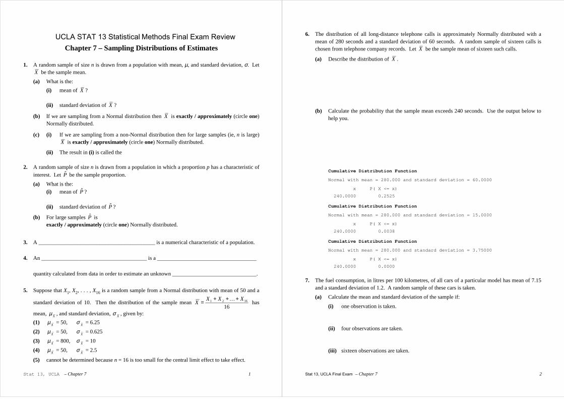
6. The distribution of all long-distance telephone calls is approximately Normally distributed with a mean of 280 seconds and a standard deviation of 60 seconds. A random sample of sixteen calls is chosen from telephone company records. Let X be the sample mean of sixteen such calls.

(a) Describe the distribution of X . (b) Calculate the probability that the sample mean exceeds 240 seconds. Use the output below to

help you.

Cumulative Distribution Function

Normal with mean = 280.000 and standard deviation = 60.0000

x P( X <= x)

240.0000 0.2525



x P( X <= x)

240.0000 0.0038



x P( X <= x)

240.0000 0.0000

7. The fuel consumption, in litres per 100 kilometres, of all cars of a particular model has mean of 7.15

and a standard deviation of 1.2. A random sample of these cars is taken.

(a) Calculate the mean and standard deviation of the sample if:

(i) one observation is taken. (ii) four observations are taken. (iii) sixteen observations are taken.


(b) In what way do your answers in (a) differ? Why?

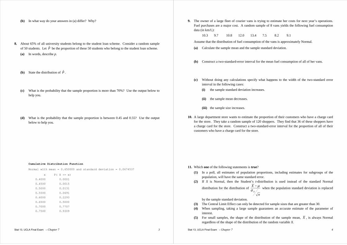
8. About 65% of all university students belong to the student loan scheme. Consider a random sample

of 50 students. Let P be the proportion of these 50 students who belong to the student loan scheme.

(a) In words, describe p. (b) State the distribution of P . (c) What is the probability that the sample proportion is more than 70%? Use the output below to

help you. (d) What is the probability that the sample proportion is between 0.45 and 0.55? Use the output

below to help you.



x P( X <= x)

0.4000 0.0001

0.4500 0.0015

0.5000 0.0131

0.5500 0.0691

0.6000 0.2293

0.6500 0.5000

0.7000 0.7707

0.7500 0.9309


9. The owner of a large fleet of courier vans is trying to estimate her costs for next year’s operations. Fuel purchases are a major cost. A random sample of 8 vans yields the following fuel consumption data (in km/L):

10.3 9.7 10.8 12.0 13.4 7.5 8.2 9.1

Assume that the distribution of fuel consumption of the vans is approximately Normal.

(a) Calculate the sample mean and the sample standard deviation. (b) Construct a two-standard-error interval for the mean fuel consumption of all of her vans.

(c) Without doing any calculations specify what happens to the width of the two-standard error interval in the following cases: (i) the sample standard deviation increases. (ii) the sample mean decreases.

(iii) the sample size increases.

10. A large department store wants to estimate the proportion of their customers who have a charge card

for the store. They take a random sample of 120 shoppers. They find that 36 of these shoppers have a charge card for the store. Construct a two-standard-error interval for the proportion of all of their customers who have a charge card for the store.

11. Which one of the following statements is true? (1) In a poll, all estimates of population proportions, including estimates for subgroups of the

population, will have the same standard error. (2) If X is Normal, then the Student’s t-distribution is used instead of the standard Normal

distribution for the distribution of

n

XXσ

µ− when the population standard deviation is replaced

by the sample standard deviation. (3) The Central Limit Effect can only be detected for sample sizes that are greater than 30. (4) When sampling, taking a large sample guarantees an accurate estimate of the parameter of

interest. (5) For small samples, the shape of the distribution of the sample mean, X , is always Normal

regardless of the shape of the distribution of the random variable X.

Stat 13 Review Chapter 8 1

UCLA Stat 13 Review Final Exam Chapter 8 – Confidence Intervals

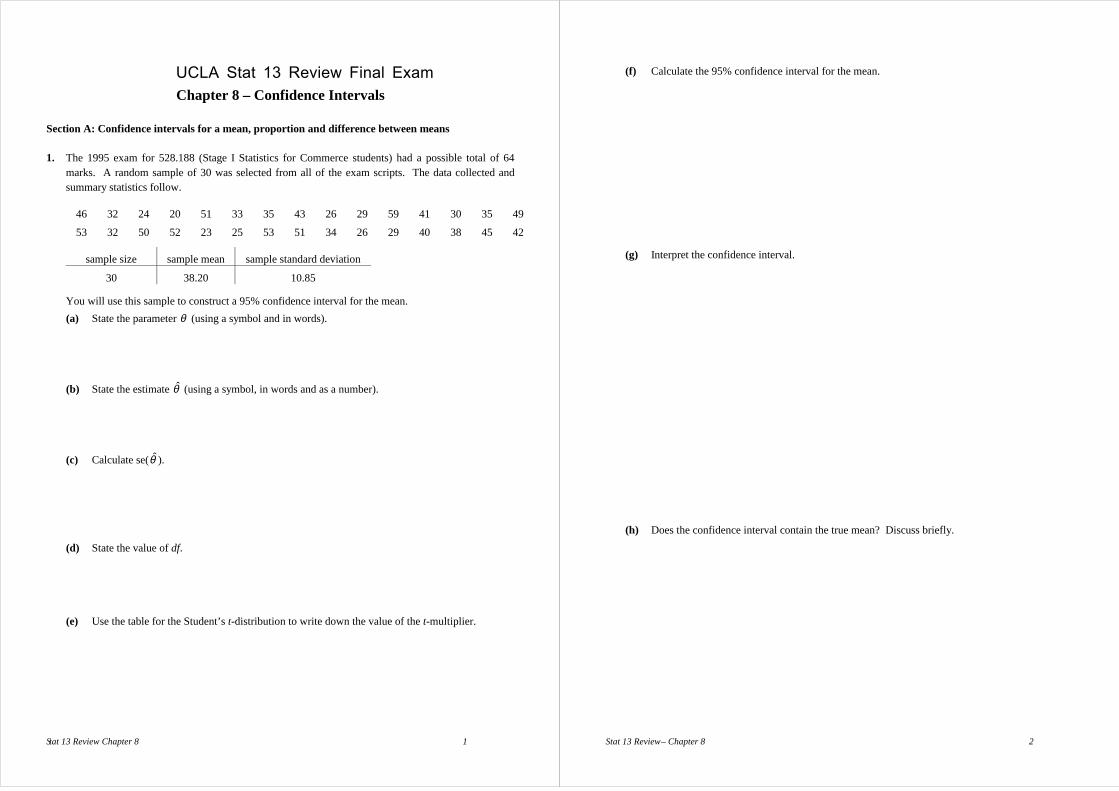
Section A: Confidence intervals for a mean, proportion and difference between means 1. The 1995 exam for 528.188 (Stage I Statistics for Commerce students) had a possible total of 64

marks. A random sample of 30 was selected from all of the exam scripts. The data collected and summary statistics follow.

46 32 24 20 51 33 35 43 26 29 59 41 30 35 49

53 32 50 52 23 25 53 51 34 26 29 40 38 45 42

sample size sample mean sample standard deviation

30 38.20 10.85

You will use this sample to construct a 95% confidence interval for the mean. (a) State the parameter θ (using a symbol and in words).

(b) State the estimate θ (using a symbol, in words and as a number).

(c) Calculate se(θ ).

(d) State the value of df.

(e) Use the table for the Student’s t-distribution to write down the value of the t-multiplier.

Stat 13 Review – Chapter 8 2

(f) Calculate the 95% confidence interval for the mean.

(g) Interpret the confidence interval.

(h) Does the confidence interval contain the true mean? Discuss briefly.

Stat 13 Review– Chapter 8 3

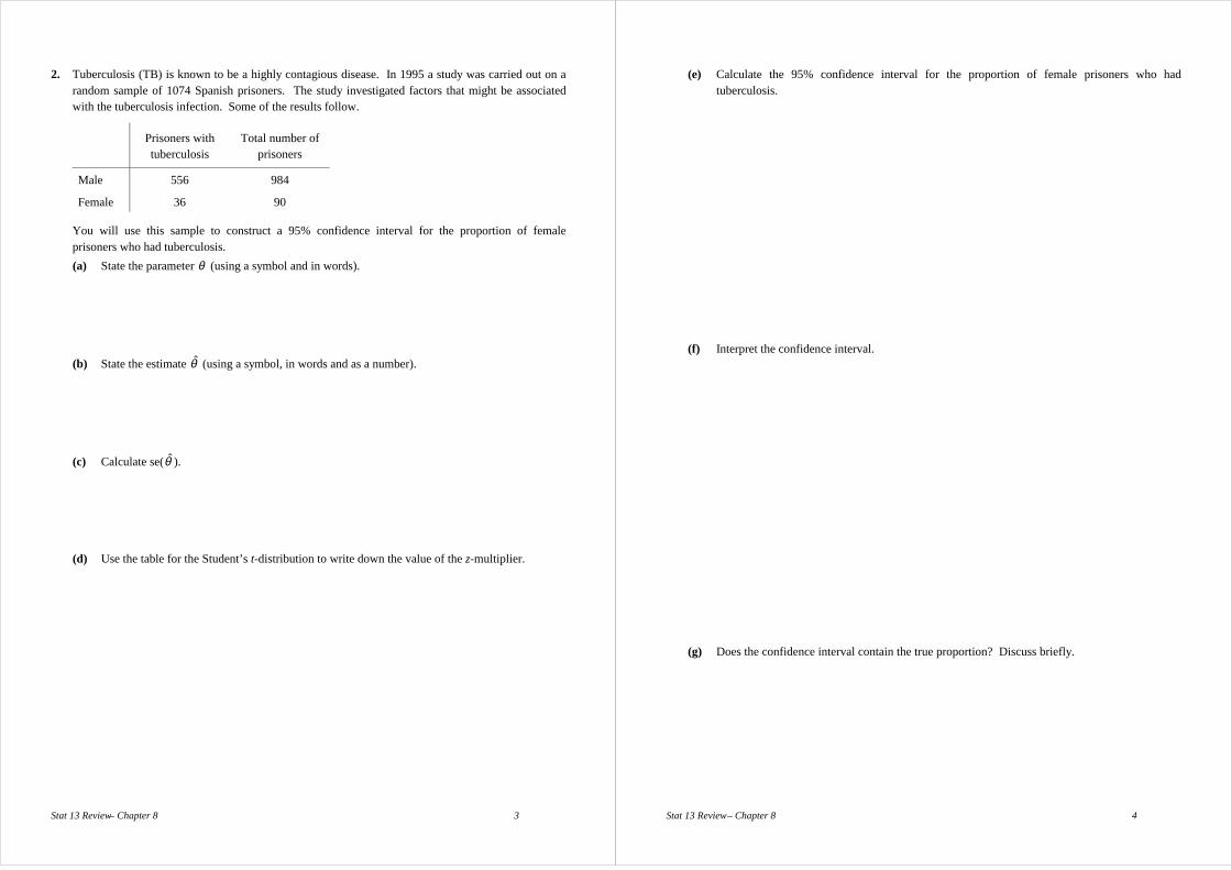
2. Tuberculosis (TB) is known to be a highly contagious disease. In 1995 a study was carried out on a random sample of 1074 Spanish prisoners. The study investigated factors that might be associated with the tuberculosis infection. Some of the results follow.

Prisoners with tuberculosis

Total number of prisoners

Male 556 984

Female 36 90

You will use this sample to construct a 95% confidence interval for the proportion of female prisoners who had tuberculosis.

(a) State the parameter θ (using a symbol and in words).

(b) State the estimate θ (using a symbol, in words and as a number).

(c) Calculate se(θ ).

(d) Use the table for the Student’s t-distribution to write down the value of the z-multiplier.


(e) Calculate the 95% confidence interval for the proportion of female prisoners who had tuberculosis.

(f) Interpret the confidence interval.

(g) Does the confidence interval contain the true proportion? Discuss briefly.


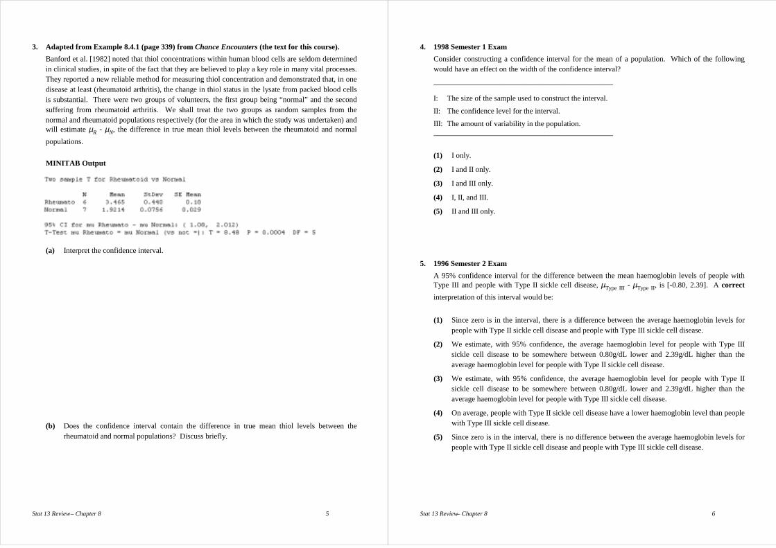
3. Adapted from Example 8.4.1 (page 339) from Chance Encounters (the text for this course). Banford et al. [1982] noted that thiol concentrations within human blood cells are seldom determined

in clinical studies, in spite of the fact that they are believed to play a key role in many vital processes. They reported a new reliable method for measuring thiol concentration and demonstrated that, in one disease at least (rheumatoid arthritis), the change in thiol status in the lysate from packed blood cells is substantial. There were two groups of volunteers, the first group being “normal” and the second suffering from rheumatoid arthritis. We shall treat the two groups as random samples from the normal and rheumatoid populations respectively (for the area in which the study was undertaken) and will estimate µR - µN, the difference in true mean thiol levels between the rheumatoid and normal populations.

MINITAB Output

(a) Interpret the confidence interval.

(b) Does the confidence interval contain the difference in true mean thiol levels between the

rheumatoid and normal populations? Discuss briefly.

Stat 13 Review– Chapter 8 6

4. 1998 Semester 1 Exam Consider constructing a confidence interval for the mean of a population. Which of the following would have an effect on the width of the confidence interval?

_______________________________________________

I: The size of the sample used to construct the interval.

II: The confidence level for the interval.

III: The amount of variability in the population. _______________________________________________

(1) I only.

(2) I and II only.

(3) I and III only.

(4) I, II, and III.

(5) II and III only.

5. 1996 Semester 2 Exam

A 95% confidence interval for the difference between the mean haemoglobin levels of people with Type III and people with Type II sickle cell disease, µType III - µType II, is [-0.80, 2.39]. A correct interpretation of this interval would be:

(1) Since zero is in the interval, there is a difference between the average haemoglobin levels for

people with Type II sickle cell disease and people with Type III sickle cell disease.

(2) We estimate, with 95% confidence, the average haemoglobin level for people with Type III sickle cell disease to be somewhere between 0.80g/dL lower and 2.39g/dL higher than the average haemoglobin level for people with Type II sickle cell disease.

(3) We estimate, with 95% confidence, the average haemoglobin level for people with Type II sickle cell disease to be somewhere between 0.80g/dL lower and 2.39g/dL higher than the average haemoglobin level for people with Type III sickle cell disease.

(4) On average, people with Type II sickle cell disease have a lower haemoglobin level than people with Type III sickle cell disease.

(5) Since zero is in the interval, there is no difference between the average haemoglobin levels for people with Type II sickle cell disease and people with Type III sickle cell disease.


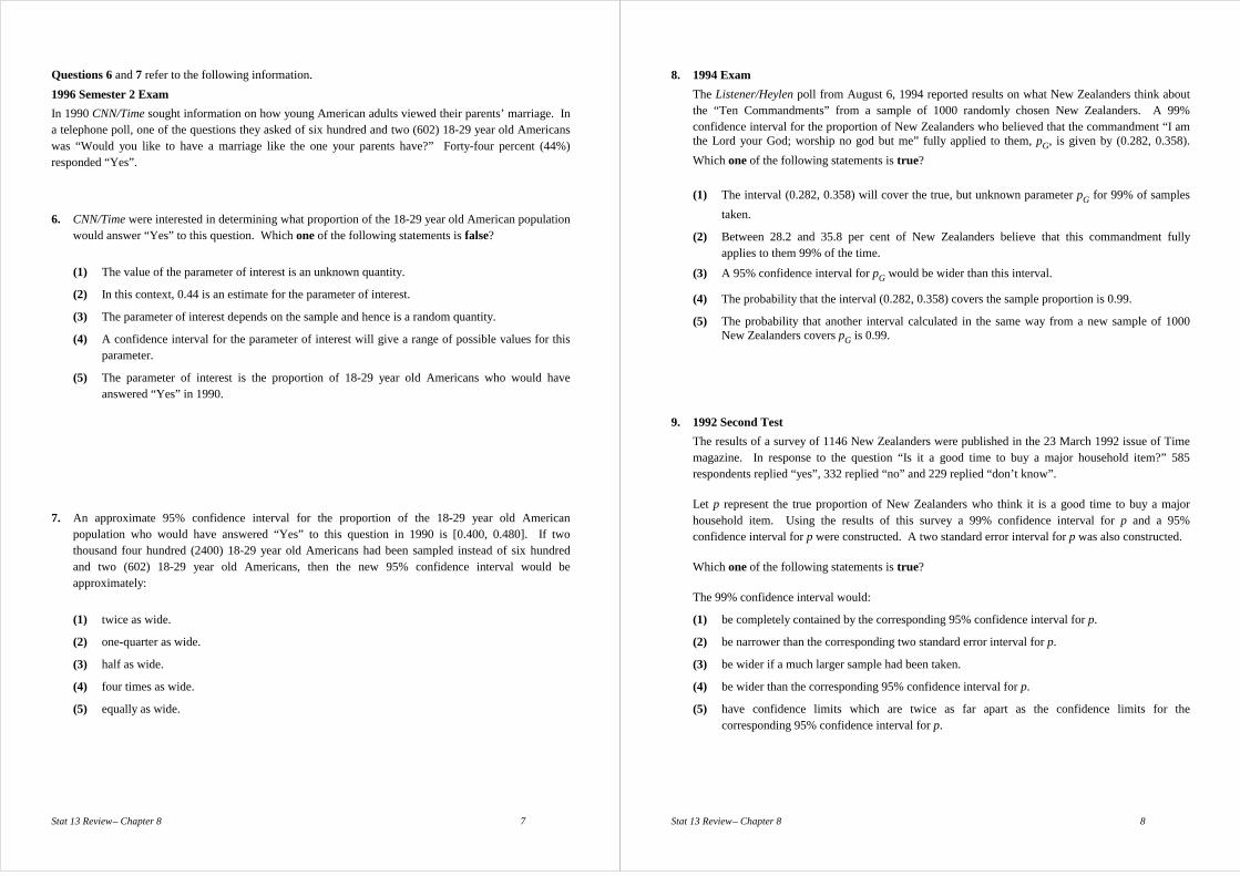
Questions 6 and 7 refer to the following information. 1996 Semester 2 Exam In 1990 CNN/Time sought information on how young American adults viewed their parents’ marriage. In a telephone poll, one of the questions they asked of six hundred and two (602) 18-29 year old Americans was “Would you like to have a marriage like the one your parents have?” Forty-four percent (44%) responded “Yes”.

6. CNN/Time were interested in determining what proportion of the 18-29 year old American population

would answer “Yes” to this question. Which one of the following statements is false?

(1) The value of the parameter of interest is an unknown quantity.

(2) In this context, 0.44 is an estimate for the parameter of interest.

(3) The parameter of interest depends on the sample and hence is a random quantity.

(4) A confidence interval for the parameter of interest will give a range of possible values for this parameter.

(5) The parameter of interest is the proportion of 18-29 year old Americans who would have answered “Yes” in 1990.

7. An approximate 95% confidence interval for the proportion of the 18-29 year old American

population who would have answered “Yes” to this question in 1990 is [0.400, 0.480]. If two thousand four hundred (2400) 18-29 year old Americans had been sampled instead of six hundred and two (602) 18-29 year old Americans, then the new 95% confidence interval would be approximately:

(1) twice as wide.

(2) one-quarter as wide.

(3) half as wide.

(4) four times as wide.

(5) equally as wide.


8. 1994 Exam The Listener/Heylen poll from August 6, 1994 reported results on what New Zealanders think about

the “Ten Commandments” from a sample of 1000 randomly chosen New Zealanders. A 99% confidence interval for the proportion of New Zealanders who believed that the commandment “I am the Lord your God; worship no god but me” fully applied to them, pG, is given by (0.282, 0.358). Which one of the following statements is true?

(1) The interval (0.282, 0.358) will cover the true, but unknown parameter pG for 99% of samples

taken.

(2) Between 28.2 and 35.8 per cent of New Zealanders believe that this commandment fully applies to them 99% of the time.

(3) A 95% confidence interval for pG would be wider than this interval.

(4) The probability that the interval (0.282, 0.358) covers the sample proportion is 0.99.

(5) The probability that another interval calculated in the same way from a new sample of 1000 New Zealanders covers pG is 0.99.

9. 1992 Second Test The results of a survey of 1146 New Zealanders were published in the 23 March 1992 issue of Time

magazine. In response to the question “Is it a good time to buy a major household item?” 585 respondents replied “yes”, 332 replied “no” and 229 replied “don’t know”.

Let p represent the true proportion of New Zealanders who think it is a good time to buy a major household item. Using the results of this survey a 99% confidence interval for p and a 95% confidence interval for p were constructed. A two standard error interval for p was also constructed. Which one of the following statements is true?

The 99% confidence interval would:

(1) be completely contained by the corresponding 95% confidence interval for p.

(2) be narrower than the corresponding two standard error interval for p.

(3) be wider if a much larger sample had been taken.

(4) be wider than the corresponding 95% confidence interval for p.

(5) have confidence limits which are twice as far apart as the confidence limits for the corresponding 95% confidence interval for p.


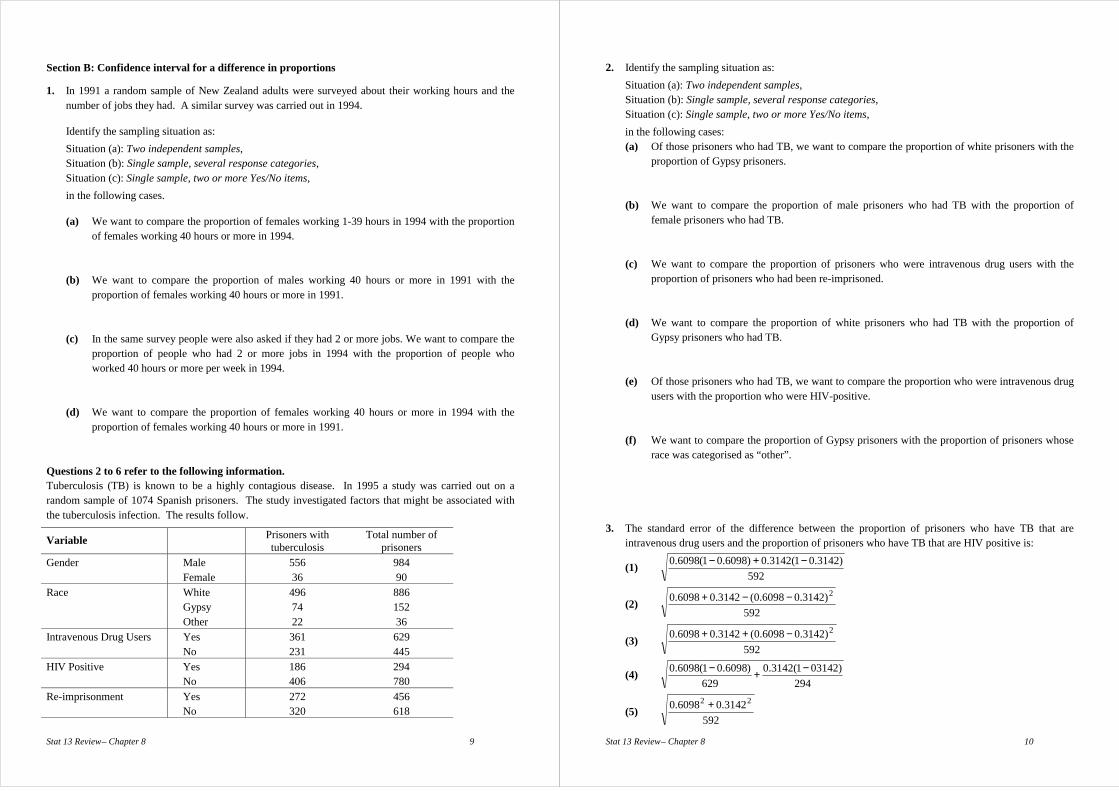
Section B: Confidence interval for a difference in proportions

1. In 1991 a random sample of New Zealand adults were surveyed about their working hours and the number of jobs they had. A similar survey was carried out in 1994.

Identify the sampling situation as: Situation (a): Two independent samples, Situation (b): Single sample, several response categories, Situation (c): Single sample, two or more Yes/No items, in the following cases.

(a) We want to compare the proportion of females working 1-39 hours in 1994 with the proportion of females working 40 hours or more in 1994.

(b) We want to compare the proportion of males working 40 hours or more in 1991 with the

proportion of females working 40 hours or more in 1991. (c) In the same survey people were also asked if they had 2 or more jobs. We want to compare the

proportion of people who had 2 or more jobs in 1994 with the proportion of people who worked 40 hours or more per week in 1994.

(d) We want to compare the proportion of females working 40 hours or more in 1994 with the

proportion of females working 40 hours or more in 1991. Questions 2 to 6 refer to the following information. Tuberculosis (TB) is known to be a highly contagious disease. In 1995 a study was carried out on a random sample of 1074 Spanish prisoners. The study investigated factors that might be associated with the tuberculosis infection. The results follow.

Variable Prisoners with tuberculosis

Total number of prisoners

Gender Male 556 984 Female 36 90 Race White 496 886 Gypsy 74 152 Other 22 36 Intravenous Drug Users Yes 361 629 No 231 445 HIV Positive Yes 186 294 No 406 780 Re-imprisonment Yes 272 456 No 320 618


2. Identify the sampling situation as: Situation (a): Two independent samples, Situation (b): Single sample, several response categories, Situation (c): Single sample, two or more Yes/No items, in the following cases: (a) Of those prisoners who had TB, we want to compare the proportion of white prisoners with the

proportion of Gypsy prisoners. (b) We want to compare the proportion of male prisoners who had TB with the proportion of

female prisoners who had TB. (c) We want to compare the proportion of prisoners who were intravenous drug users with the

proportion of prisoners who had been re-imprisoned. (d) We want to compare the proportion of white prisoners who had TB with the proportion of

Gypsy prisoners who had TB. (e) Of those prisoners who had TB, we want to compare the proportion who were intravenous drug

users with the proportion who were HIV-positive. (f) We want to compare the proportion of Gypsy prisoners with the proportion of prisoners whose

race was categorised as “other”. 3. The standard error of the difference between the proportion of prisoners who have TB that are

intravenous drug users and the proportion of prisoners who have TB that are HIV positive is:

(1) 592

)3142.01(3142.0)6098.01(6098.0 −+−

(2) 592

)3142.06098.0(3142.06098.0 2−−+

(3) 592

)3142.06098.0(3142.06098.0 2−++

(4) 294

)031421(3142.0629

)6098.01(6098.0 −+−

(5) 592

3142.06098.0 22 +


4. Construct a 95% confidence interval for the difference between the proportion of White prisoners who were infected with TB and the proportion of Gypsy prisoners who were infected with TB. State what your interval tells you in plain English.

(a) State the parameter θ (using symbols and in words). (b) State the estimate θ (using symbols, in words and as a number). (c) Calculate se(θ ). (d) Use the table for the Student’s t-distribution to write down the value of the z-multiplier. (e) Calculate the confidence interval. (f) Interpret the confidence interval.


5. Construct a 95% confidence interval for the difference in the proportion of prisoners infected with TB who were white and the proportion of prisoners infected with TB who were Gypsy.

(a) State the parameter θ (using symbols and in words). (b) State the estimate θ (using symbols, in words and as a number). (c) Calculate se(θ ). (d) Use the table for the Student’s t-distribution to write down the value of the z-multiplier. (e) Calculate the confidence interval. (f) Interpret the confidence interval.


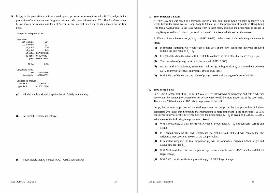
6. Let pY be the proportion of intravenous drug user prisoners who were infected with TB, and pN be the proportion of non-intravenous drug user prisoners who were infected with TB. The Excel worksheet below shows the calculations for a 95% confidence interval based on the data shown on the first page.

Two population proportions

Input data

X1_sample 361 X2_sample 231

n1_total 629 n2_total 445 p1_ratio 0.573926868 p2_ratio 0.519101124

pdiff 0.054825744

Alpha 0.05

Calculated value se 0.03081794

t-multiplier 1.959961082

Confidence Interval Lower limit -0.00557622 Upper limit 0.115227708

(a) Which sampling situation applies here? Briefly explain why.

(b) Interpret the confidence interval.

(c) Is it plausible that pY is equal to pN? Justify your answer.


7. 1997 Semester 2 Exam A Time/CNN poll was based on a telephone survey of 800 adult Hong Kong residents conducted two weeks before the hand over of Hong Kong to China. pc is the proportion of people in Hong Kong who think “Corruption” is the issue which worries them most, and pf is the proportion of people in Hong Kong who think “Reduced personal freedoms” is the issue which worries them most.

A 95% confidence interval for pc – pf is (0.012, 0.088). Which one of the following statements is

false?

(1) In repeated sampling, we would expect that 95% of the 95% confidence intervals produced contain the true value of pc – pf.

(2) In light of the data, the interval (0.012, 0.088) contains the most plausible values for pc – pf.

(3) The true value of pc – pf must be in the interval (0.012, 0.088).

(4) At this level of confidence, statements such as “pc is bigger than pf by somewhere between 0.012 and 0.088” are true, on average, 19 out of 20 times.

(5) With 95% confidence, the true value of pc – pf is 0.05 with a margin of error of ±0.038.

8. 1995 Second Test In a Time Morgan poll (July 1994) 662 voters were interviewed by telephone and asked whether

developing the economy or protecting the environment would be more important in the short term. There were 238 National and 162 Labour supporters in the poll.

Let pN be the true proportion of National supporters and let pL be the true proportion of Labour

supporters who think that protecting the environment is more important in the short term. A 95% confidence interval for the difference between the proportions pN - pL is given by [-0.1526, 0.0326]. Which one of the following interpretations is true?

(1) With a probability of 0.95, the true difference of proportions pN - pL lies between –0.1526 and 0.0326.

(2) In repeated sampling the 95% confidence interval [-0.1526, 0.0326] will contain the true difference in proportions in 95% of the samples taken.

(3) In repeated sampling the true proportion pN will be somewhere between 0.1526 larger and 0.0326 smaller than pL.

(4) With 95% confidence the true proportion pN is somewhere between 0.1526 smaller and 0.0326 larger than pL.

(5) With 95% confidence the true proportion pN is 0.1852 larger than pL.


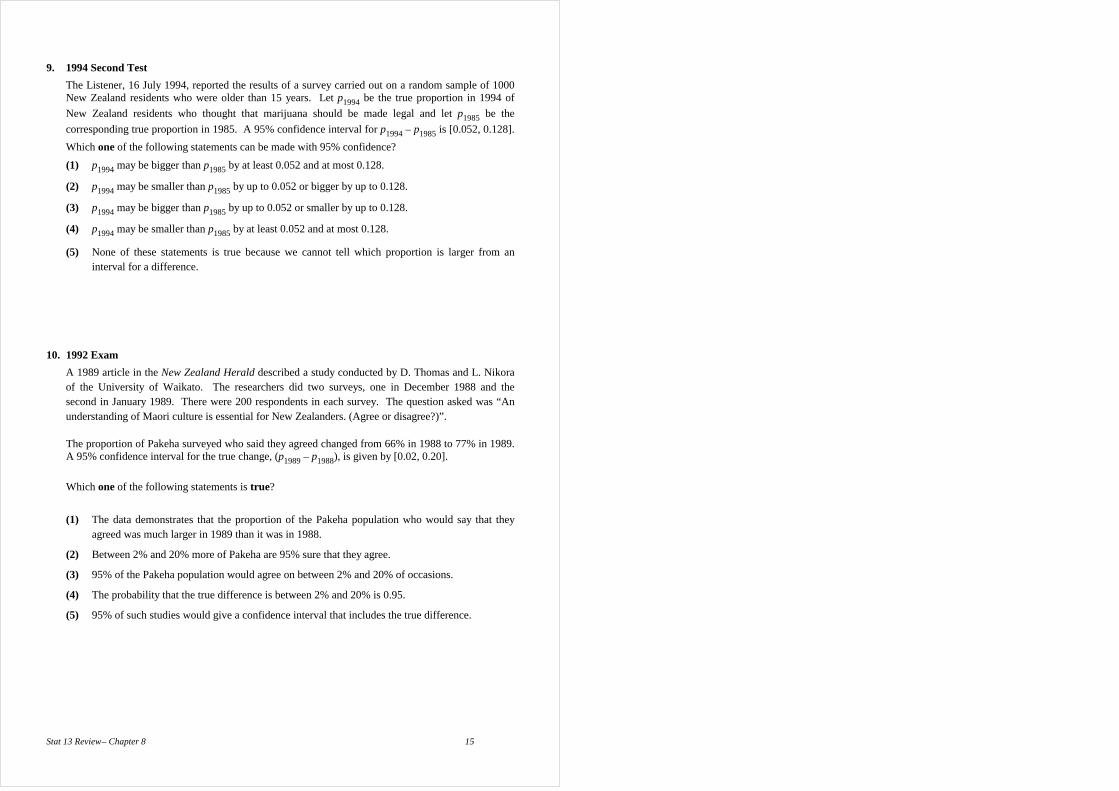
9. 1994 Second Test The Listener, 16 July 1994, reported the results of a survey carried out on a random sample of 1000

New Zealand residents who were older than 15 years. Let p1994 be the true proportion in 1994 of New Zealand residents who thought that marijuana should be made legal and let p1985 be the corresponding true proportion in 1985. A 95% confidence interval for p1994 – p1985 is [0.052, 0.128]. Which one of the following statements can be made with 95% confidence?

(1) p1994 may be bigger than p1985 by at least 0.052 and at most 0.128.

(2) p1994 may be smaller than p1985 by up to 0.052 or bigger by up to 0.128.

(3) p1994 may be bigger than p1985 by up to 0.052 or smaller by up to 0.128.

(4) p1994 may be smaller than p1985 by at least 0.052 and at most 0.128.

(5) None of these statements is true because we cannot tell which proportion is larger from an interval for a difference.

10. 1992 Exam A 1989 article in the New Zealand Herald described a study conducted by D. Thomas and L. Nikora

of the University of Waikato. The researchers did two surveys, one in December 1988 and the second in January 1989. There were 200 respondents in each survey. The question asked was “An understanding of Maori culture is essential for New Zealanders. (Agree or disagree?)”.

The proportion of Pakeha surveyed who said they agreed changed from 66% in 1988 to 77% in 1989.

A 95% confidence interval for the true change, (p1989 – p1988), is given by [0.02, 0.20]. Which one of the following statements is true?

(1) The data demonstrates that the proportion of the Pakeha population who would say that they agreed was much larger in 1989 than it was in 1988.

(2) Between 2% and 20% more of Pakeha are 95% sure that they agree.

(3) 95% of the Pakeha population would agree on between 2% and 20% of occasions.

(4) The probability that the true difference is between 2% and 20% is 0.95.

(5) 95% of such studies would give a confidence interval that includes the true difference.


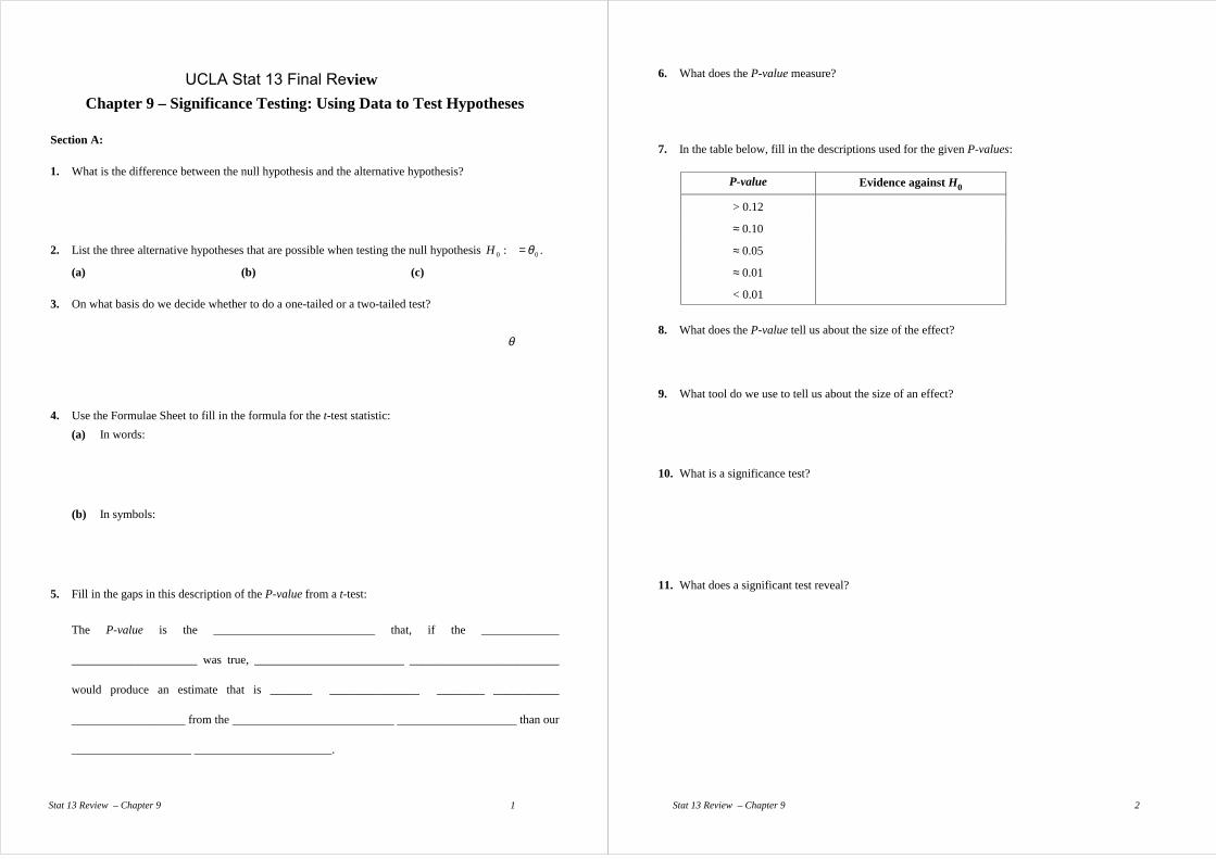
UCLA Stat 13 Final Review Chapter 9 – Significance Testing: Using Data to Test Hypotheses

Section A: 1. What is the difference between the null hypothesis and the alternative hypothesis? 2. List the three alternative hypotheses that are possible when testing the null hypothesis 00 : θ

θ

=H .

(a) (b) (c) 3. On what basis do we decide whether to do a one-tailed or a two-tailed test? 4. Use the Formulae Sheet to fill in the formula for the t-test statistic: (a) In words: (b) In symbols: 5. Fill in the gaps in this description of the P-value from a t-test:

The P-value is the ___________________________ that, if the _____________

_____________________ was true, _________________________ _________________________

would produce an estimate that is _______ _______________ ________ ___________

___________________ from the ___________________________ ____________________ than our

____________________ _______________________.


6. What does the P-value measure?

7. In the table below, fill in the descriptions used for the given P-values:

P-value Evidence against H0

> 0.12

≈ 0.10

≈ 0.05

≈ 0.01

< 0.01

8. What does the P-value tell us about the size of the effect? 9. What tool do we use to tell us about the size of an effect? 10. What is a significance test? 11. What does a significant test reveal?

Stat 13, Review – Chapter 9 3

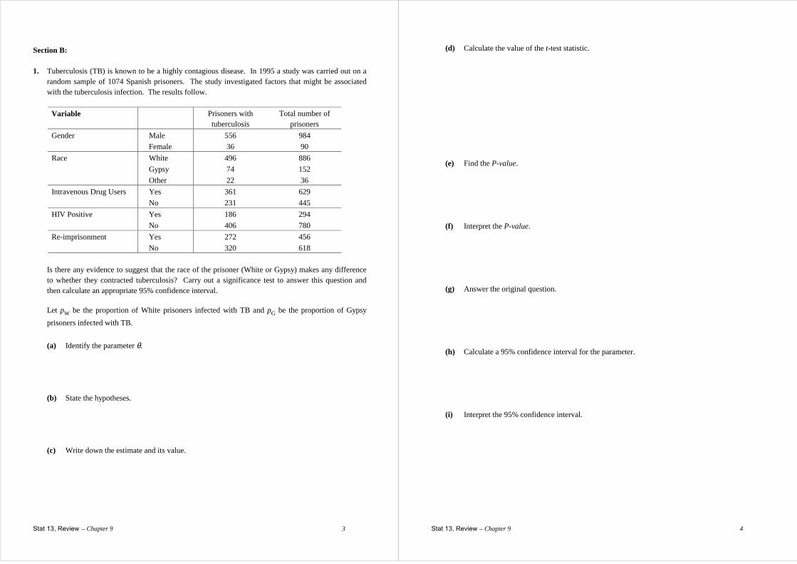
Section B: 1. Tuberculosis (TB) is known to be a highly contagious disease. In 1995 a study was carried out on a

random sample of 1074 Spanish prisoners. The study investigated factors that might be associated with the tuberculosis infection. The results follow.

Variable Prisoners with

tuberculosis Total number of

prisoners Gender Male 556 984 Female 36 90 Race White 496 886 Gypsy 74 152 Other 22 36 Intravenous Drug Users Yes 361 629 No 231 445 HIV Positive Yes 186 294 No 406 780 Re-imprisonment Yes 272 456 No 320 618

Is there any evidence to suggest that the race of the prisoner (White or Gypsy) makes any difference

to whether they contracted tuberculosis? Carry out a significance test to answer this question and then calculate an appropriate 95% confidence interval.

Let pW be the proportion of White prisoners infected with TB and pG be the proportion of Gypsy

prisoners infected with TB.

(a) Identify the parameter θ. (b) State the hypotheses. (c) Write down the estimate and its value.


(d) Calculate the value of the t-test statistic. (e) Find the P-value. (f) Interpret the P-value. (g) Answer the original question. (h) Calculate a 95% confidence interval for the parameter. (i) Interpret the 95% confidence interval.


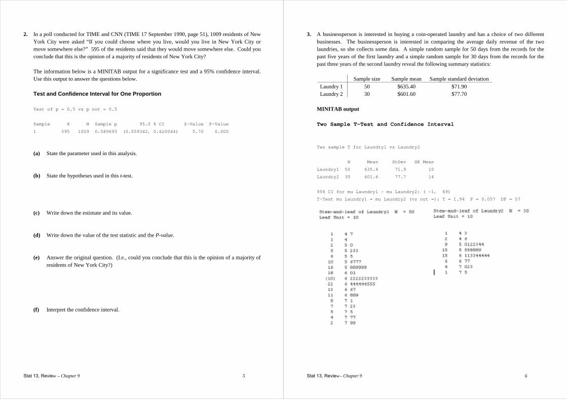
2. In a poll conducted for TIME and CNN (TIME 17 September 1990, page 51), 1009 residents of New York City were asked “If you could choose where you live, would you live in New York City or move somewhere else?” 595 of the residents said that they would move somewhere else. Could you conclude that this is the opinion of a majority of residents of New York City?

The information below is a MINITAB output for a significance test and a 95% confidence interval.

Use this output to answer the questions below.

Test and Confidence Interval for One Proportion Test of p = 0.5 vs p not = 0.5

Sample X N Sample p 95.0 % CI Z-Value P-Value

1 595 1009 0.589693 (0.559342, 0.620044) 5.70 0.000

(a) State the parameter used in this analysis. (b) State the hypotheses used in this t-test. (c) Write down the estimate and its value. (d) Write down the value of the test statistic and the P-value. (e) Answer the original question. (I.e., could you conclude that this is the opinion of a majority of

residents of New York City?) (f) Interpret the confidence interval.


3. A businessperson is interested in buying a coin-operated laundry and has a choice of two different businesses. The businessperson is interested in comparing the average daily revenue of the two laundries, so she collects some data. A simple random sample for 50 days from the records for the past five years of the first laundry and a simple random sample for 30 days from the records for the past three years of the second laundry reveal the following summary statistics:

Sample size Sample mean Sample standard deviation Laundry 1 50 $635.40 $71.90 Laundry 2 30 $601.60 $77.70

MINITAB output Two Sample T-Test and Confidence Interval

Two sample T for Laundry1 vs Laundry2

N Mean StDev SE Mean

Laundry1 50 635.4 71.9 10

Laundry2 30 601.6 77.7 14

95% CI for mu Laundry1 - mu Laundry2: ( -1, 69)

T-Test mu Laundry1 = mu Laundry2 (vs not =): T = 1.94 P = 0.057 DF = 57


(a) State the parameter used in this analysis. (b) State the hypotheses used in this t-test. (c) Write down the estimate and its value. (d) Write down the value of the test statistic. (e) Interpret the test. (f) Interpret the confidence interval. (g) Do the stem-and-leaf plots give you any reasons for doubting the validity of the results of this

analysis? Briefly explain. (h) If this analysis were done by hand the value of df would have been 29. Why does the output

show that df = 57?


Section C: 1. Which one of the following statements regarding significance testing is false? (1) A highly significant test result means that the size of the difference between the estimated value

of the parameter and the hypothesised value of the parameter is significant in a practical sense.

(2) A P-value of less than 0.01 is often referred to as a highly significant test result.

(3) A nonsignificant test result does not necessarily mean H0 is true.

(4) A two-tail test of H0: θ = θ0 is significant at the 5% significance level if and only if θ0 lies outside a 95% confidence interval for θ.

(5) Testing at the 5% level of significance means that the null hypothesis is rejected whenever a P-value smaller than 5% is obtained.

2. Which one of the following statements is false? (1) In hypothesis testing, a nonsignificant result implies that H0 is true.

(2) In hypothesis testing, a two-tail test should be used when the idea for doing the test has been triggered by the data.

(3) In surveys, the nonsampling error is often greater than the sampling error.

(4) Larger sample sizes lead to smaller standard errors.

(5) In hypothesis testing, statistical significance does not necessarily imply practical significance. 3. Which one of the following statements regarding significance testing is false? (1) Formal tests can help determine whether effects we see in our data may just be due to sampling

variation.

(2) The P-value associated with a two-sided alternative hypothesis is obtained by doubling the P-value associated with a one-sided alternative hypothesis.

(3) The P-value says nothing about the size of an effect.

(4) The data should be carefully examined in order to determine whether the alternative hypothesis needs to be one-sided or two-sided.

(5) The P-value describes the strength of evidence against the null hypothesis.

UCLA Stat 13 Review – Chapter 10 1

UCLA Stat 13 Final Exam Review Chapter 10 – Data on a Continuous Variable

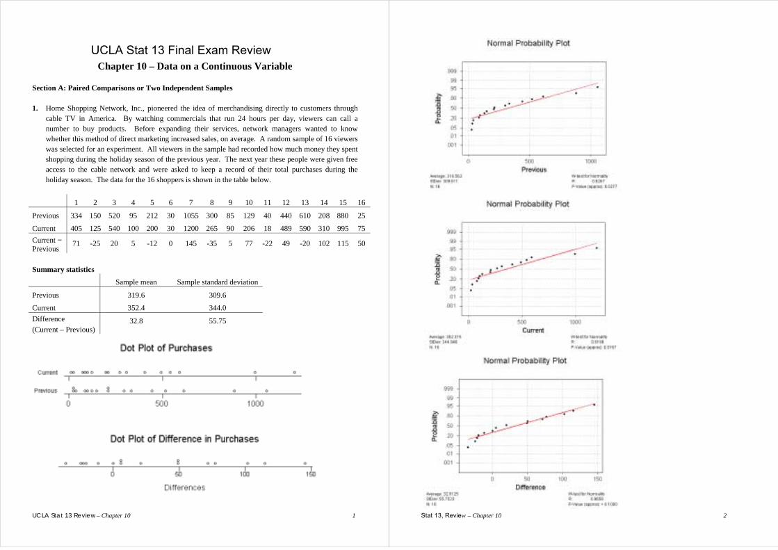
Section A: Paired Comparisons or Two Independent Samples 1. Home Shopping Network, Inc., pioneered the idea of merchandising directly to customers through

cable TV in America. By watching commercials that run 24 hours per day, viewers can call a number to buy products. Before expanding their services, network managers wanted to know whether this method of direct marketing increased sales, on average. A random sample of 16 viewers was selected for an experiment. All viewers in the sample had recorded how much money they spent shopping during the holiday season of the previous year. The next year these people were given free access to the cable network and were asked to keep a record of their total purchases during the holiday season. The data for the 16 shoppers is shown in the table below.

1 2 3 4 5 6 7 8 9 10 11 12 13 14 15 16

Previous 334 150 520 95 212 30 1055 300 85 129 40 440 610 208 880 25

Current 405 125 540 100 200 30 1200 265 90 206 18 489 590 310 995 75 Current − Previous

71 -25 20 5 -12 0 145 -35 5 77 -22 49 -20 102 115 50

Summary statistics Sample mean Sample standard deviation

Previous 319.6 309.6

Current 352.4 344.0 Difference (Current – Previous)

32.8 55.75



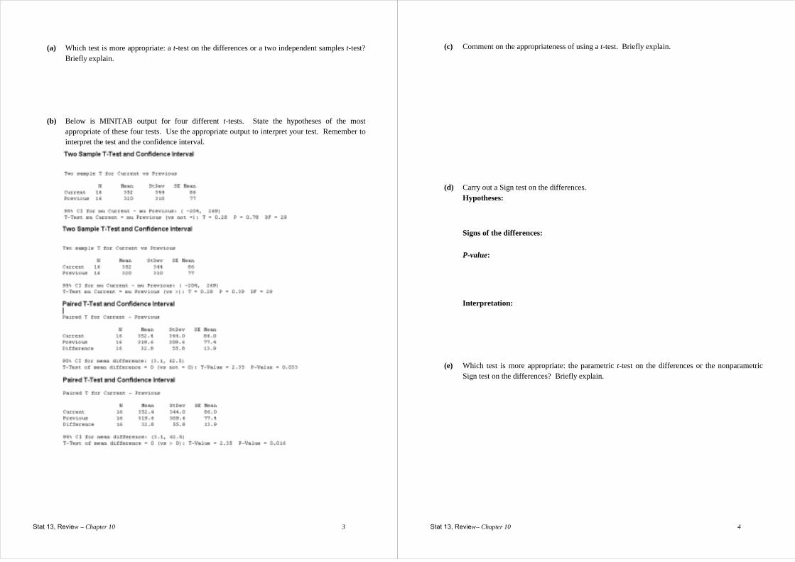
(a) Which test is more appropriate: a t-test on the differences or a two independent samples t-test? Briefly explain.

(b) Below is MINITAB output for four different t-tests. State the hypotheses of the most

appropriate of these four tests. Use the appropriate output to interpret your test. Remember to interpret the test and the confidence interval.


(c) Comment on the appropriateness of using a t-test. Briefly explain.

(d) Carry out a Sign test on the differences. Hypotheses:

Signs of the differences:

P-value:

Interpretation:

(e) Which test is more appropriate: the parametric t-test on the differences or the nonparametric

Sign test on the differences? Briefly explain.


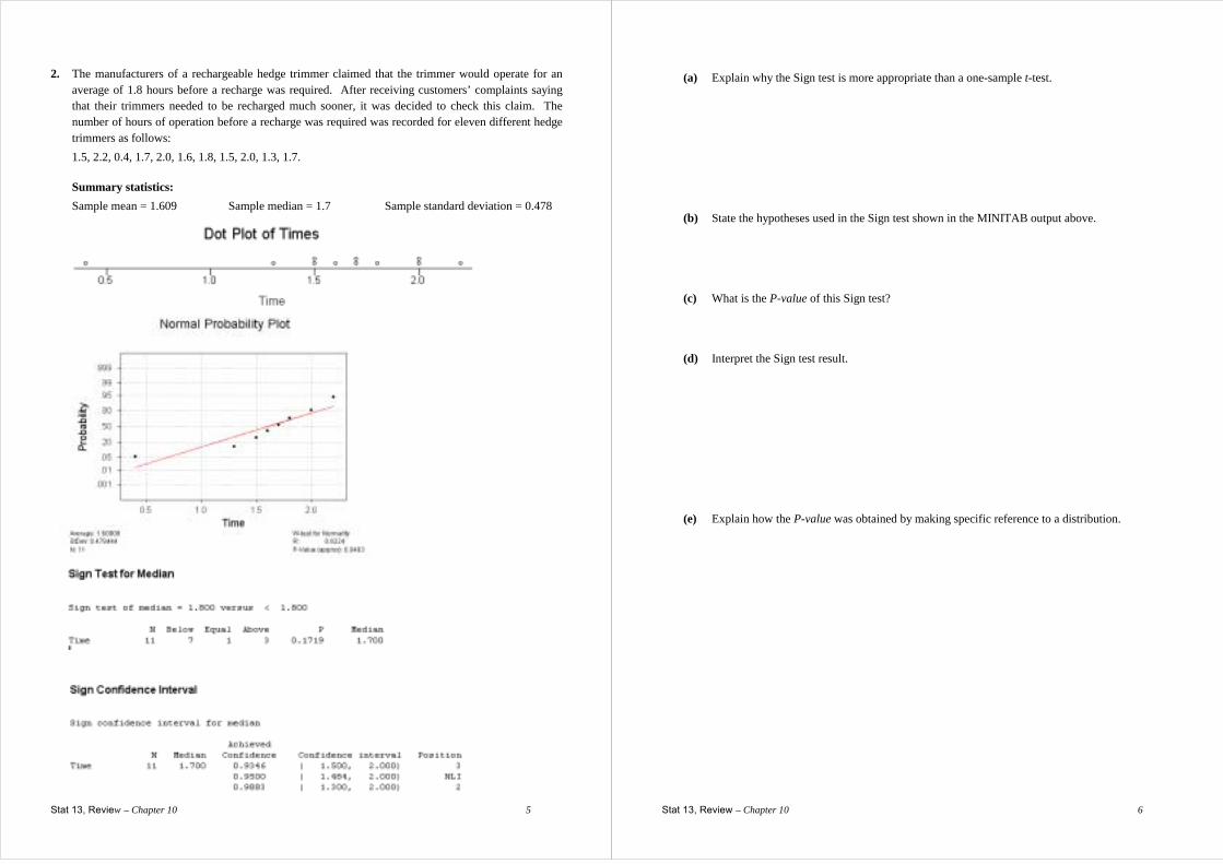
2. The manufacturers of a rechargeable hedge trimmer claimed that the trimmer would operate for an average of 1.8 hours before a recharge was required. After receiving customers’ complaints saying that their trimmers needed to be recharged much sooner, it was decided to check this claim. The number of hours of operation before a recharge was required was recorded for eleven different hedge trimmers as follows:

1.5, 2.2, 0.4, 1.7, 2.0, 1.6, 1.8, 1.5, 2.0, 1.3, 1.7.

Summary statistics: Sample mean = 1.609 Sample median = 1.7 Sample standard deviation = 0.478


(a) Explain why the Sign test is more appropriate than a one-sample t-test.

(b) State the hypotheses used in the Sign test shown in the MINITAB output above.

(c) What is the P-value of this Sign test?

(d) Interpret the Sign test result.

(e) Explain how the P-value was obtained by making specific reference to a distribution.


Section B: More Than Two Independent Samples 1. (a) What is another name for the F-test? (b) When do we consider using an F-test? (c) What are the hypotheses for a four independent samples F-test? (d) (i) List the assumptions for an F-test. (ii) Describe how we check them.


2. (a) What formula is given in the formulae sheet for calculating the value of the F-test statistic, f0? (b) What are 2

Bs and 2Ws called and what do they measure?

3. In the following cases state the number of samples, k, and the total sample size, ntot. (a) df1 = 5, df2 = 10 (b) df1 = 8, df2 = 144 (c) df1 = 4, df2 = 25


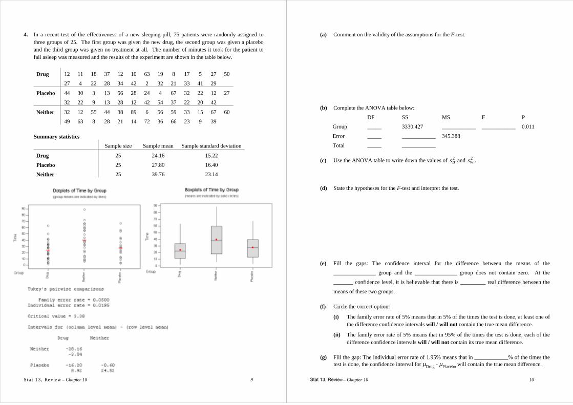
4. In a recent test of the effectiveness of a new sleeping pill, 75 patients were randomly assigned to three groups of 25. The first group was given the new drug, the second group was given a placebo and the third group was given no treatment at all. The number of minutes it took for the patient to fall asleep was measured and the results of the experiment are shown in the table below.

Drug 12 11 18 37 12 10 63 19 8 17 5 27 50

27 4 22 28 34 42 2 32 21 33 41 29

Placebo 44 30 3 13 56 28 24 4 67 32 22 12 27

32 22 9 13 28 12 42 54 37 22 20 42

Neither 32 12 55 44 38 89 6 56 59 33 15 67 60

49 63 8 28 21 14 72 36 66 23 9 39 Summary statistics

Sample size Sample mean Sample standard deviation

Drug 25 24.16 15.22

Placebo 25 27.80 16.40

Neither 25 39.76 23.14


(a) Comment on the validity of the assumptions for the F-test.

(b) Complete the ANOVA table below:

DF SS MS F P

Group _____ 3330.427 ____________ ____________ 0.011

Error _____ ____________ 345.388

Total _____ ____________ (c) Use the ANOVA table to write down the values of 2

Bs and 2Ws .

(d) State the hypotheses for the F-test and interpret the test.

(e) Fill the gaps: The confidence interval for the difference between the means of the

_______________ group and the _______________ group does not contain zero. At the

_______ confidence level, it is believable that there is _________ real difference between the

means of these two groups. (f) Circle the correct option:

(i) The family error rate of 5% means that in 5% of the times the test is done, at least one of the difference confidence intervals will / will not contain the true mean difference.

(ii) The family error rate of 5% means that in 95% of the times the test is done, each of the difference confidence intervals will / will not contain its true mean difference.

(g) Fill the gap: The individual error rate of 1.95% means that in ____________% of the times the

test is done, the confidence interval for µDrug - µPlacebo will contain the true mean difference.


Section C: Experimental Design For each of the situations below write a brief report in which you: • Describe an experiment you could use to investigate the problem posed. Include details of how you

would allocate treatments to subjects. Justify your choice of experimental design. • Describe the hypotheses you would test. • List all the assumptions that should be satisfied so that your chosen method is valid. 1. In the early 1990s, aspirin, well known as a mild painkiller, was recognised to have blood-thinning

properties. If a small dosage of aspirin is taken regularly, the risk of a heart attack caused by blood clotting can be reduced substantially. A drug company in the United States is presently interested in testing a new drug which it believes has similar properties to aspirin. A total of 19,000 people will take part in the study. The number of deaths due to heart attacks will be recorded over a 10-year period.


2. An orchardist in Napier is concerned about the presence of a species of (hungry!) bugs that have infested the apple trees in his orchard. There are four different sprays available that will eliminate this pest and the orchardist wants to test the effectiveness of these to see which one, if any, is worth using. There are 80 apple trees that are infested with the bug. Two weeks after spraying, the orchardist will take a random sample of 100 leaves from each of the 80 trees and count the number of these leaves that have bugs on them.


3. A market research company has been contracted to carry out a large survey. The survey involves asking a detailed series of questions that usually takes between 15 to 25 minutes to answer. The company is aware that the longer it takes to answer the questionnaire, the less likely people are to complete the survey. They wish to conduct a small pilot study to investigate which of two designs of the questionnaire will take the least time to answer. They have 5 interviewers available to interview 50 subjects for the pilot study.

Stat 13, Review Chapter 10 14

4. A researcher is to conduct an experiment to examine the effect if digitalis on the contraction of heart muscles of rats. Digitalis is a drug commonly used in humans to control the heart rate. The researcher has twenty fresh rat hearts available for the experiment, each of which is sliced into two halves. Two different drug dosages of digitalis are to be applied to the pieces of heart muscle and the resulting strength of the muscle contractions recorded. Various factors, such as the age and physical health of the rats at time of death, will affect the resulting muscle contractions after the digitalis has been applied.


Section D: Quiz 1. (a) What should you always do first to any dataset? (b) Why? 2. When carrying out hypothesis tests (both parametric and nonparametric) we use sample data. What

assumption is made about this sample data? 3. From the list below, select the assumptions required for the stated test. (i) Underlying distribution(s) is (are) Normal. (ii) Independence between samples. (iii) Independence between pairs of observations. (iv) Independence between observations. (v) Equal population standard deviations. (vi) Equal sample sizes. (vii) Equal sample means. (a) One sample t-test.


(b) One sample Sign test. (c) One sample t-test on the differences (from paired-comparison data). (d) Two sample t-test. (e) F-test. 4. What should you do if there appears to be an outlier present? 5. What is useful about a nonparametric test? 6. What is a drawback of using a nonparametric test rather than its parametric equivalent test?


UCLA Stat 13 Final Exam Review Chapter 11 – Tables of Counts

Section A: One-way Tables

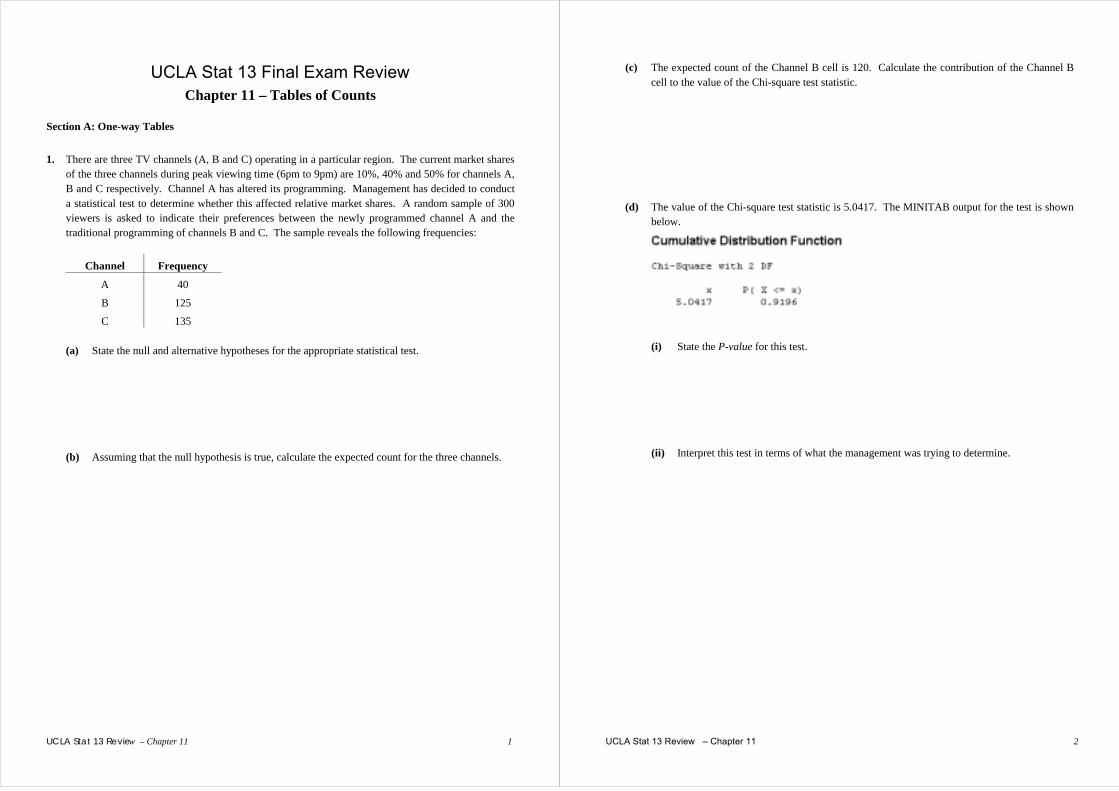
1. There are three TV channels (A, B and C) operating in a particular region. The current market shares

of the three channels during peak viewing time (6pm to 9pm) are 10%, 40% and 50% for channels A, B and C respectively. Channel A has altered its programming. Management has decided to conduct a statistical test to determine whether this affected relative market shares. A random sample of 300 viewers is asked to indicate their preferences between the newly programmed channel A and the traditional programming of channels B and C. The sample reveals the following frequencies:

Channel Frequency

A 40

B 125

C 135 (a) State the null and alternative hypotheses for the appropriate statistical test.

(b) Assuming that the null hypothesis is true, calculate the expected count for the three channels.


(c) The expected count of the Channel B cell is 120. Calculate the contribution of the Channel B cell to the value of the Chi-square test statistic.

(d) The value of the Chi-square test statistic is 5.0417. The MINITAB output for the test is shown

below.

(i) State the P-value for this test.

(ii) Interpret this test in terms of what the management was trying to determine.

UCCLA Stat 13 Review – Chapter 11 3

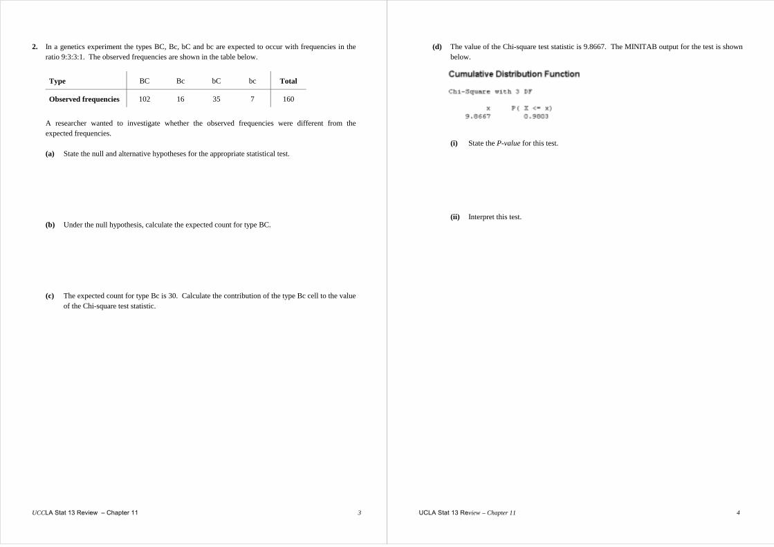
2. In a genetics experiment the types BC, Bc, bC and bc are expected to occur with frequencies in the ratio 9:3:3:1. The observed frequencies are shown in the table below.

Type BC Bc bC bc Total

Observed frequencies 102 16 35 7 160

A researcher wanted to investigate whether the observed frequencies were different from the

expected frequencies. (a) State the null and alternative hypotheses for the appropriate statistical test. (b) Under the null hypothesis, calculate the expected count for type BC. (c) The expected count for type Bc is 30. Calculate the contribution of the type Bc cell to the value

of the Chi-square test statistic.


(d) The value of the Chi-square test statistic is 9.8667. The MINITAB output for the test is shown below.

(i) State the P-value for this test.

(ii) Interpret this test.


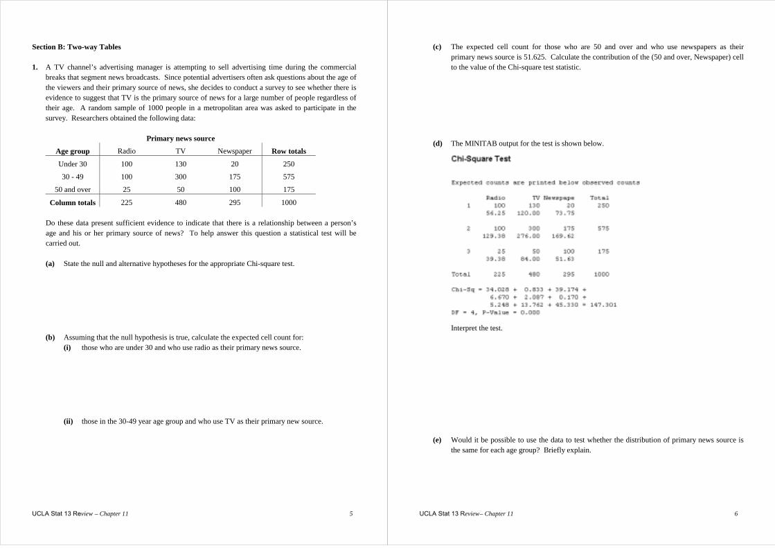
Section B: Two-way Tables 1. A TV channel’s advertising manager is attempting to sell advertising time during the commercial

breaks that segment news broadcasts. Since potential advertisers often ask questions about the age of the viewers and their primary source of news, she decides to conduct a survey to see whether there is evidence to suggest that TV is the primary source of news for a large number of people regardless of their age. A random sample of 1000 people in a metropolitan area was asked to participate in the survey. Researchers obtained the following data:

Primary news source

Age group Radio TV Newspaper Row totals

Under 30 100 130 20 250

30 - 49 100 300 175 575

50 and over 25 50 100 175

Column totals 225 480 295 1000

Do these data present sufficient evidence to indicate that there is a relationship between a person’s age and his or her primary source of news? To help answer this question a statistical test will be carried out. (a) State the null and alternative hypotheses for the appropriate Chi-square test.

(b) Assuming that the null hypothesis is true, calculate the expected cell count for: (i) those who are under 30 and who use radio as their primary news source.

(ii) those in the 30-49 year age group and who use TV as their primary new source.


(c) The expected cell count for those who are 50 and over and who use newspapers as their primary news source is 51.625. Calculate the contribution of the (50 and over, Newspaper) cell to the value of the Chi-square test statistic.

(d) The MINITAB output for the test is shown below.

Interpret the test.

(e) Would it be possible to use the data to test whether the distribution of primary news source is

the same for each age group? Briefly explain.


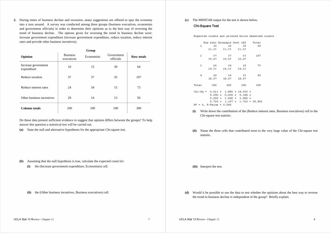
2. During times of business decline and recession, many suggestions are offered to spur the economy into a turn around. A survey was conducted among three groups (business executives, economists and government officials) in order to determine their opinions as to the best way of reversing the trend of business decline. The options given for reversing the trend in business decline were: increase government expenditure (increase government expenditure, reduce taxation, reduce interest rates and provide other business incentives).

Group

Opinion Business executives

Economists Government officials Row totals

Increase government expenditure

10 15 39 64

Reduce taxation 37 37 33 107

Reduce interest rates 24 34 15 73

Other business incentives 29 14 13 56

Column totals 100 100 100 300

Do these data present sufficient evidence to suggest that opinion differs between the groups? To help answer this question a statistical test will be carried out. (a) State the null and alternative hypotheses for the appropriate Chi-square test.

(b) Assuming that the null hypothesis is true, calculate the expected count for: (i) the (Increase government expenditure, Economists) cell.

(ii) the (Other business incentives, Business executives) cell.


(c) The MINITAB output for the test is shown below.

(i) Write down the contribution of the (Reduce interest rates, Business executives) cell to the Chi-square test statistic.

(ii) Name the three cells that contributed most to the very large value of the Chi-square test

statsitic.

(iii) Interpret the test.

(d) Would it be possible to use the data to test whether the opinions about the best way to reverse

the trend in business decline is independent of the group? Briefly explain.


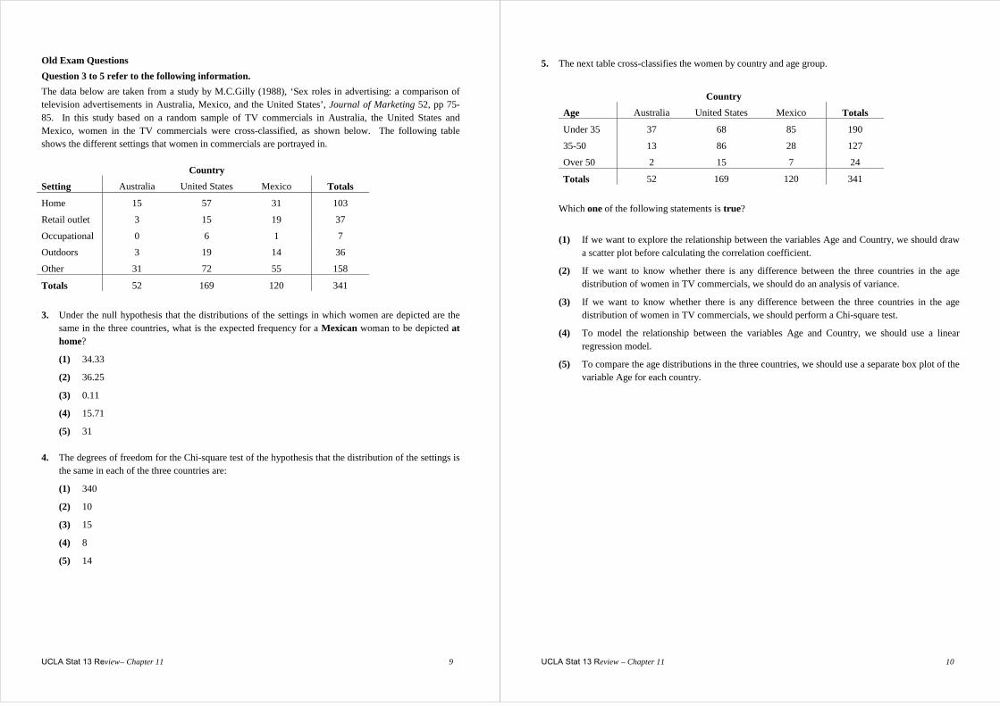
Old Exam Questions Question 3 to 5 refer to the following information. The data below are taken from a study by M.C.Gilly (1988), ‘Sex roles in advertising: a comparison of television advertisements in Australia, Mexico, and the United States’, Journal of Marketing 52, pp 75-85. In this study based on a random sample of TV commercials in Australia, the United States and Mexico, women in the TV commercials were cross-classified, as shown below. The following table shows the different settings that women in commercials are portrayed in. Country

Setting Australia United States Mexico Totals

Home 15 57 31 103

Retail outlet 3 15 19 37

Occupational 0 6 1 7

Outdoors 3 19 14 36

Other 31 72 55 158

Totals 52 169 120 341

3. Under the null hypothesis that the distributions of the settings in which women are depicted are the

same in the three countries, what is the expected frequency for a Mexican woman to be depicted at home?

(1) 34.33

(2) 36.25

(3) 0.11

(4) 15.71

(5) 31 4. The degrees of freedom for the Chi-square test of the hypothesis that the distribution of the settings is

the same in each of the three countries are:

(1) 340

(2) 10

(3) 15

(4) 8

(5) 14


5. The next table cross-classifies the women by country and age group.

Country

Age Australia United States Mexico Totals

Under 35 37 68 85 190

35-50 13 86 28 127

Over 50 2 15 7 24

Totals 52 169 120 341

Which one of the following statements is true?

(1) If we want to explore the relationship between the variables Age and Country, we should draw a scatter plot before calculating the correlation coefficient.

(2) If we want to know whether there is any difference between the three countries in the age distribution of women in TV commercials, we should do an analysis of variance.

(3) If we want to know whether there is any difference between the three countries in the age distribution of women in TV commercials, we should perform a Chi-square test.

(4) To model the relationship between the variables Age and Country, we should use a linear regression model.

(5) To compare the age distributions in the three countries, we should use a separate box plot of the variable Age for each country.


Review UCLA Stat 13 Final Chapter 12 – Relationships between Quantitative Variables:

Regression and Correlation

Section A: The Straight Line Graph 1. The equation of a line is of the form xy 10 ββ += , where 0β is the y-intercept and 1β is the slope of

the line. Give the values of 0β and 1β for the following lines. (a) y = 5 + 3x (b) y = 10 – 14x 0β = 0β = 1β = 1β = 2. (a) What is the equation of a line that has a slope of 2 and a y-intercept of −3? (b) By how much does the y-value of this line change when (i) x is increased by 1? (ii) x is increased by 6?


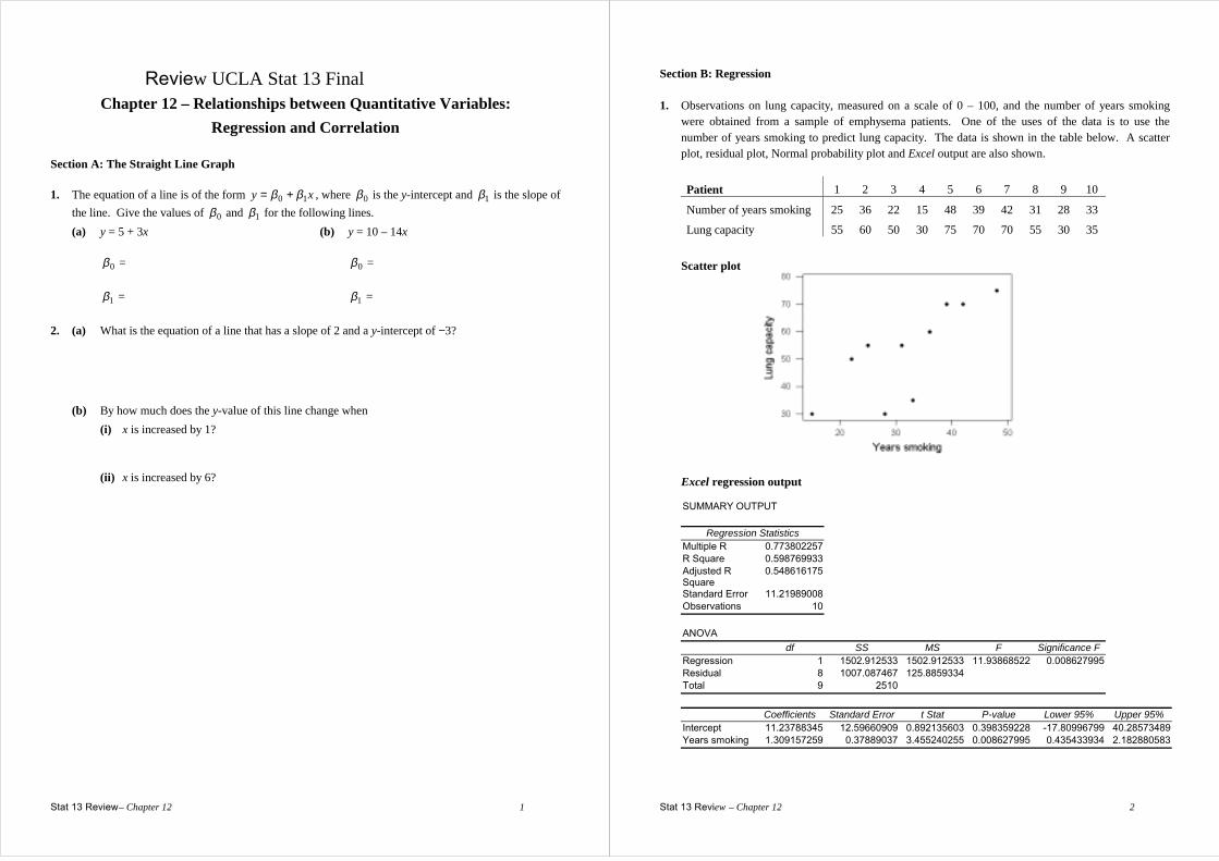
Section B: Regression 1. Observations on lung capacity, measured on a scale of 0 – 100, and the number of years smoking

were obtained from a sample of emphysema patients. One of the uses of the data is to use the number of years smoking to predict lung capacity. The data is shown in the table below. A scatter plot, residual plot, Normal probability plot and Excel output are also shown.

Patient 1 2 3 4 5 6 7 8 9 10

Number of years smoking 25 36 22 15 48 39 42 31 28 33

Lung capacity 55 60 50 30 75 70 70 55 30 35

Scatter plot

Excel regression output

SUMMARY OUTPUT

Regression Statistics Multiple R 0.773802257 R Square 0.598769933 Adjusted R Square

0.548616175

Standard Error 11.21989008 Observations 10

ANOVA

df SS MS F Significance F Regression 1 1502.912533 1502.912533 11.93868522 0.008627995 Residual 8 1007.087467 125.8859334 Total 9 2510

Coefficients Standard Error t Stat P-value Lower 95% Upper 95%

Intercept 11.23788345 12.59660909 0.892135603 0.398359228 -17.80996799 40.28573489 Years smoking 1.309157259 0.37889037 3.455240255 0.008627995 0.435433934 2.182880583


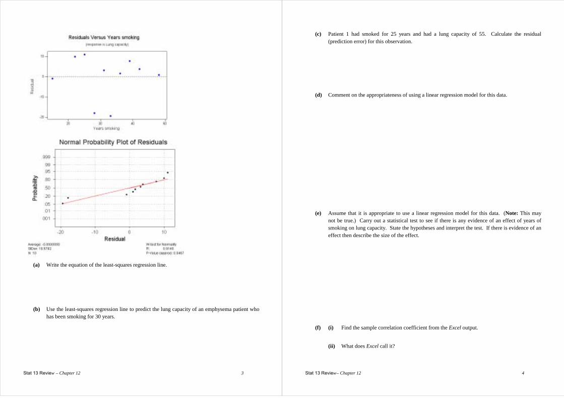
(a) Write the equation of the least-squares regression line.

(b) Use the least-squares regression line to predict the lung capacity of an emphysema patient who

has been smoking for 30 years.


(c) Patient 1 had smoked for 25 years and had a lung capacity of 55. Calculate the residual (prediction error) for this observation.

(d) Comment on the appropriateness of using a linear regression model for this data.

(e) Assume that it is appropriate to use a linear regression model for this data. (Note: This may

not be true.) Carry out a statistical test to see if there is any evidence of an effect of years of smoking on lung capacity. State the hypotheses and interpret the test. If there is evidence of an effect then describe the size of the effect.

(f) (i) Find the sample correlation coefficient from the Excel output.

(ii) What does Excel call it?


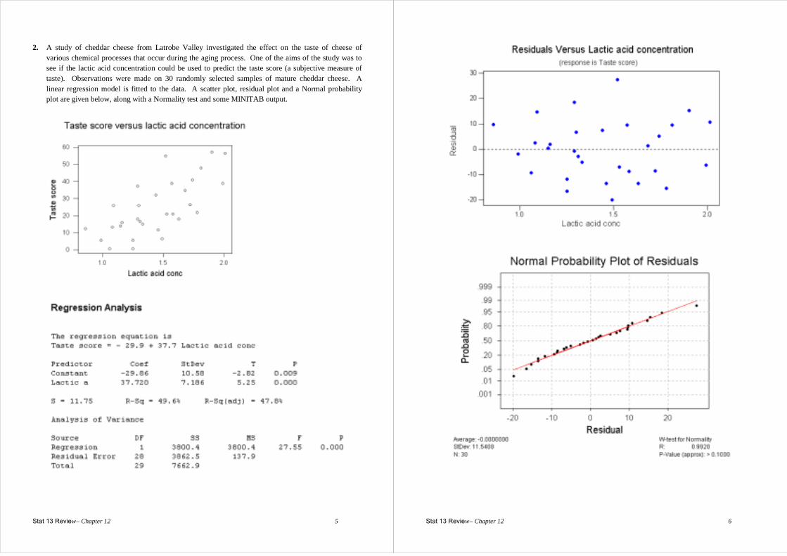
2. A study of cheddar cheese from Latrobe Valley investigated the effect on the taste of cheese of various chemical processes that occur during the aging process. One of the aims of the study was to see if the lactic acid concentration could be used to predict the taste score (a subjective measure of taste). Observations were made on 30 randomly selected samples of mature cheddar cheese. A linear regression model is fitted to the data. A scatter plot, residual plot and a Normal probability plot are given below, along with a Normality test and some MINITAB output.



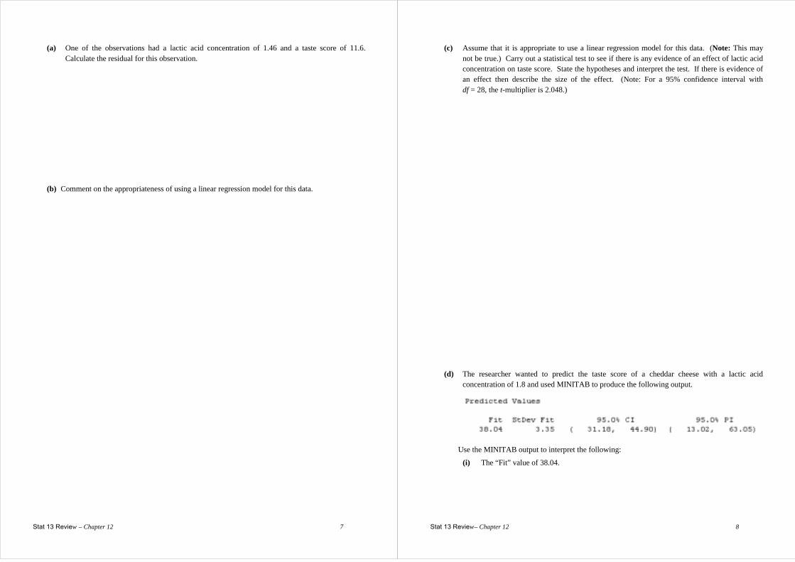
(a) One of the observations had a lactic acid concentration of 1.46 and a taste score of 11.6. Calculate the residual for this observation.

(b) Comment on the appropriateness of using a linear regression model for this data.


(c) Assume that it is appropriate to use a linear regression model for this data. (Note: This may not be true.) Carry out a statistical test to see if there is any evidence of an effect of lactic acid concentration on taste score. State the hypotheses and interpret the test. If there is evidence of an effect then describe the size of the effect. (Note: For a 95% confidence interval with df = 28, the t-multiplier is 2.048.)

(d) The researcher wanted to predict the taste score of a cheddar cheese with a lactic acid

concentration of 1.8 and used MINITAB to produce the following output.

Use the MINITAB output to interpret the following:

(i) The “Fit” value of 38.04.


(ii) The 95% confidence interval.

(iii) The 95% prediction interval.

(e) The fitted least-squares regression line indicates that for each increase of 0.05 in lactic acid

concentration we expect that, on average, the taste score will:

(1) increase by approximately 1.9 units.

(2) decrease by approximately 28.0 units.



(5) decrease by approximately 29.9 units.

(f) The fitted least-squares regression line can be used to predict taste scores for samples of mature

cheddar from the Latrobe Valley. Cheese that has a lactic acid concentration of 1.30 has a predicted taste score of:

(1) 24.5

(2) 19.2

(3) 49.0

(4) 78.9

(5) 25.9


Section C: Old Exam Questions 1. Which one of the following statements regarding the sample correlation coefficient, r, is false?

(1) The value of r is an indication of the strength of linear association between the two variables.

(2) In the calculation of the value of r, it does not matter which one of the variables is designated as X and which one is designated as Y.

(3) If the sample correlation coefficient equals 1, then there is a perfect linear association between the two variables for these observations.

(4) The value of r must be between 0 and 1 inclusive.

(5) The value of r may be near 0 when there is a non-linear relationship between the two variables. 2. In the theory of inference, which one of the following is not an assumption for the linear regression

model? (1) The mean of the errors is 0 for all X-values.

(2) The errors are not independent.

(3) The standard deviation of the errors is the same for all X-values.

(4) The relationship between X and Y variables can be summarised by a straight line.

(5) The distribution of the errors is Normal for all X-values. 3. Consider using a scatter plot to investigate the relationship between a response variable Y and an

explanatory variable X. The scatter plot indicates that there is a strong, negative, linear relationship between X and Y and that there are no outliers in the data. Which one of the following statements is false? (1) The trend line explains most of the differences we see between the values of Y in the scatter

plot.

(2) There are no points that are unusually far from the trend curve.

(3) Y changes, on average, by a fixed amount for each unit change in X.

(4) The value of Y tends to decrease as the value of X increases.

(5) If a new scatter plot was produced that only used a limited range of the X-values, then the relationship would look stronger.

4. Which one of the following statements regarding the sample correlation coefficient, r, is false?

(1) A value of r near 1 does not necessarily mean there is a causal relationship between the two variables.

(2) The value of r cannot be less than -1.

(3) In calculating r, it is not necessary to define one of the random variables as the response and the other as the explanatory variable.

(4) A negative value of r indicates a negative association between the two variables.

(5) A value of r equal to 0 indicates that there is no relationship between the two variables.


5. Which one of the following statements regarding linear regression and correlation analysis is false? (1) In an analysis of the correlation between two variables, we do not single out either variable to

have a special role.

(2) Using regression techniques, we can never determine whether a causal relationship exists between two variables.

(3) An outlier on a scatter plot should be removed if it is found to be an error.

(4) A strong relationship plotted for a limited range of x-values may appear weaker than it actually is.

(5) The least-squares regression technique minimises the sum of the squared prediction errors. 6. Which one of the following statements is not an assumption of the linear regression model?

(1) The relationship between the X variable and the Y variable is linear.

(2) All random errors are independent.

(3) The X-values are Normally distributed.

(4) The standard deviation of the random errors does not depend on the X-values.

(5) For any X-value, the random errors are Normally distributed (with a mean of 0). 7. Which one of the following statements about the sample correlation coefficient, r, between two

variables X and Y is false? (1) A value of r close to 1 implies a causal relationship exists between X and Y.

(2) A value of r = 0 does not necessarily mean that X and Y are unrelated.

(3) A value of r = 0 indicates that no linear relationship exists between X and Y.

(4) A value of r = 1 indicates that a perfect positive linear relationship exists between X and Y.

(5) A value of r = -1 indicates that a perfect negative linear relationship exists between X and Y. 8. Which one of the following statements about linear regression and correlation is false?

(1) A regression relationship is of the form: observation = trend + residual scatter. (2) In analyses of the correlation type, no variables are singled out to have a special role; all

variables are treated symmetrically.

(3) Correlation coefficients provide a better means of detecting a relationship between two continuous variables than a scatter plot.

(4) The fitted trend line is often useful for prediction purposes.

(5) Lines fitted to data using the least-squares method do not allow us to reliably predict the behaviour of Y outside the range of x-values for which we have collected data.


9. Which one of the following statements is false? (1) The two main components of a regression relationship are ‘trend’ and ‘scatter’.

(2) The larger the amount of scatter, the smaller the size of the absolute value of the correlation coefficient, r.

(3) A correlation coefficient of r = 0 means that there is no linear relationship between the two variables, whereas a negative correlation coefficient indicates an association, the strength of which depends on its absolute value.

(4) A small value of the absolute value of the correlation coefficient, r, indicates a weak linear relationship.

(5) In the interpretation of a correlation coefficient, r, one variable is always treated as the response variable and the other as the explanatory variable.

10. Which one of the following statements concerning the analysis of residuals is false? (1) A linear regression model should never be used without first examining the appropriate scatter

plot.

(2) Outliers in the values of the explanatory variable can have a big influence on the fitted regression line.

(3) The residuals are computed to be ii yx ˆ− .

(4) If the assumption of constant error standard deviation is valid, we would expect to see a patternless horizontal band in a plot of the residuals versus the explanatory variable.

(5) We can investigate the distribution of the errors by looking at a stem-and-leaf plot of a hjistogram of the residuals.


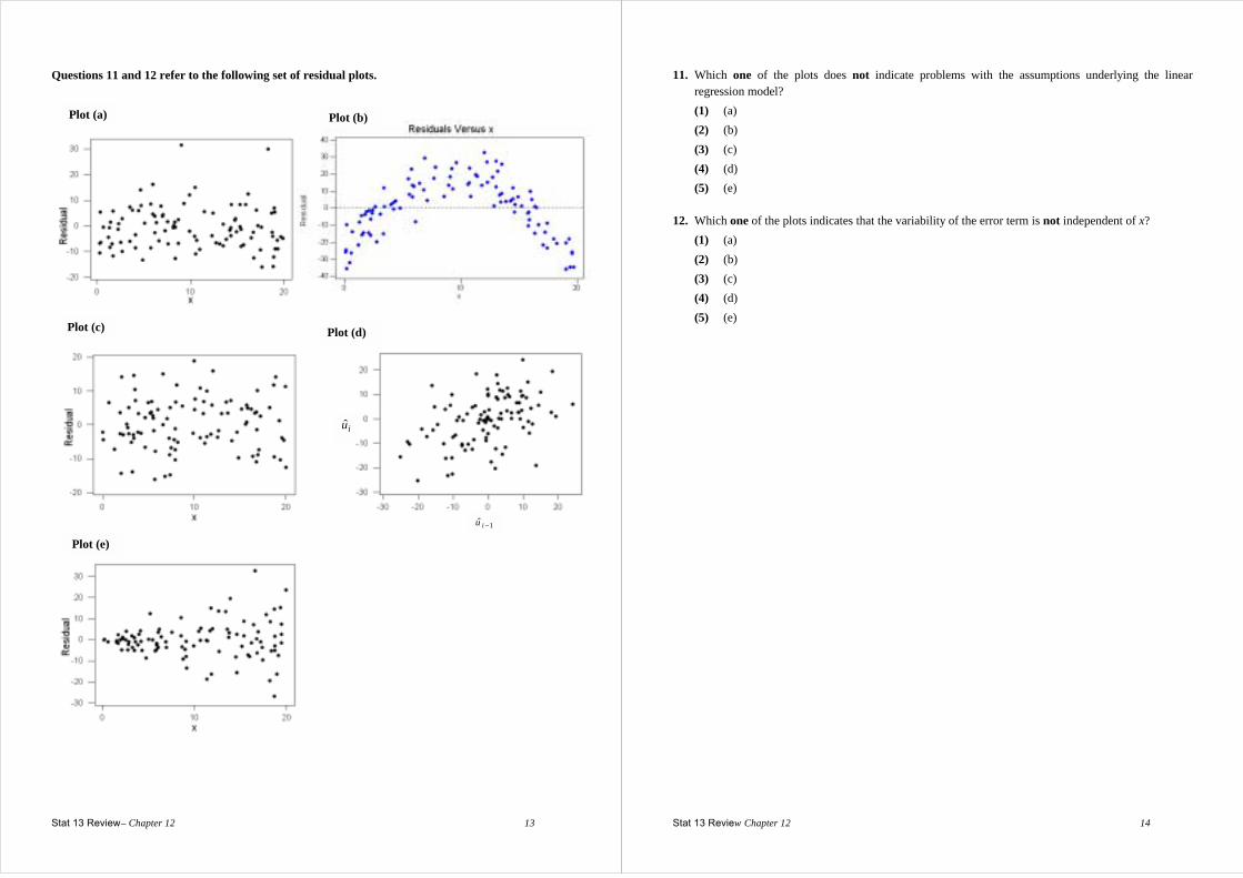
Questions 11 and 12 refer to the following set of residual plots.

Plot (a) Plot (b)

Plot (c)

1ˆ −iu

iu

Plot (d)

Plot (e)

Stat 13 Review Chapter 12 14

11. Which one of the plots does not indicate problems with the assumptions underlying the linear regression model?

(1) (a) (2) (b) (3) (c) (4) (d) (5) (e) 12. Which one of the plots indicates that the variability of the error term is not independent of x? (1) (a) (2) (b) (3) (c) (4) (d) (5) (e)

Documents

Chapter 7 – Sampling Distributions of Estimates X X Xdinov/courses_students.dir/STAT13_Fall01/STAT13... · Chapter 7 – Sampling Distributions of Estimates 1. ... standard deviation