١

Chapter 5 Statistical Models in Simulation

Banks, Carson, Nelson & NicolDiscrete-Event System Simulation

٢

Purpose & Overview

The world the model-builder sees is probabilistic rather than deterministic.

Some statistical model might well describe the variations.

An appropriate model can be developed by sampling the phenomenon of interest:

Select a known distribution through educated guessesMake estimate of the parameter(s)Test for goodness of fit

In this chapter:Review several important probability distributionsPresent some typical application of these models

٢

٣

Review of Terminology and Concepts

In this section, we will review the following concepts:

Discrete random variablesContinuous random variablesCumulative distribution functionExpectation

٤

Discrete Random Variables [Probability Review]

X is a discrete random variable if the number of possible values of X is finite, or countably infinite.Example: Consider jobs arriving at a job shop.

Let X be the number of jobs arriving each week at a job shop.Rx = possible values of X (range space of X) = {0,1,2,…}p(xi) = probability the random variable is xi = P(X = xi)

p(xi), i = 1,2, … must satisfy:

The collection of pairs [xi, p(xi)], i = 1,2,…, is called the probability distribution of X, and p(xi) is called the probability mass function (pmf) of X.

∑∞

==

≥

11)( 2.

allfor ,0)( 1.

i i

i

xp

ixp

٣

٥

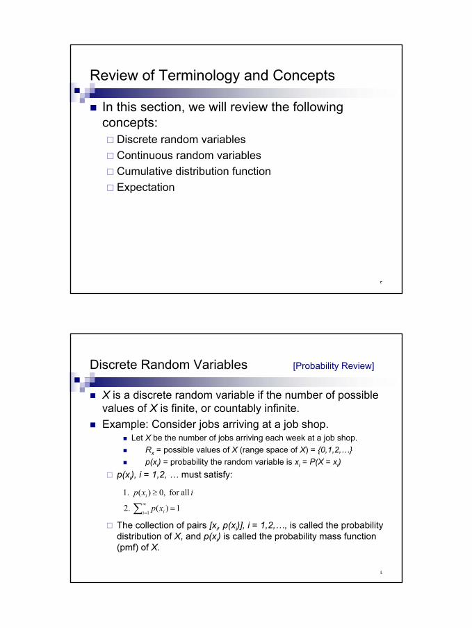
Continuous Random Variables [Probability Review]

X is a continuous random variable if its range space Rx is an interval or a collection of intervals.The probability that X lies in the interval [a,b] is given by:

f(x), denoted as the pdf of X, satisfies:

PropertiesX

R

X

Rxxf

dxxf

Rxxf

X

in not is if ,0)( 3.

1)( 2.

in allfor , 0)( 1.

=

=

≥

∫

∫=≤≤b

adxxfbXaP )()(

)()()()( .2

0)( because ,0)( 1. 0

00

bXaPbXaPbXaPbXaP

dxxfxXPx

x

pppp =≤=≤=≤≤

=== ∫

٦

Continuous Random Variables [Probability Review]

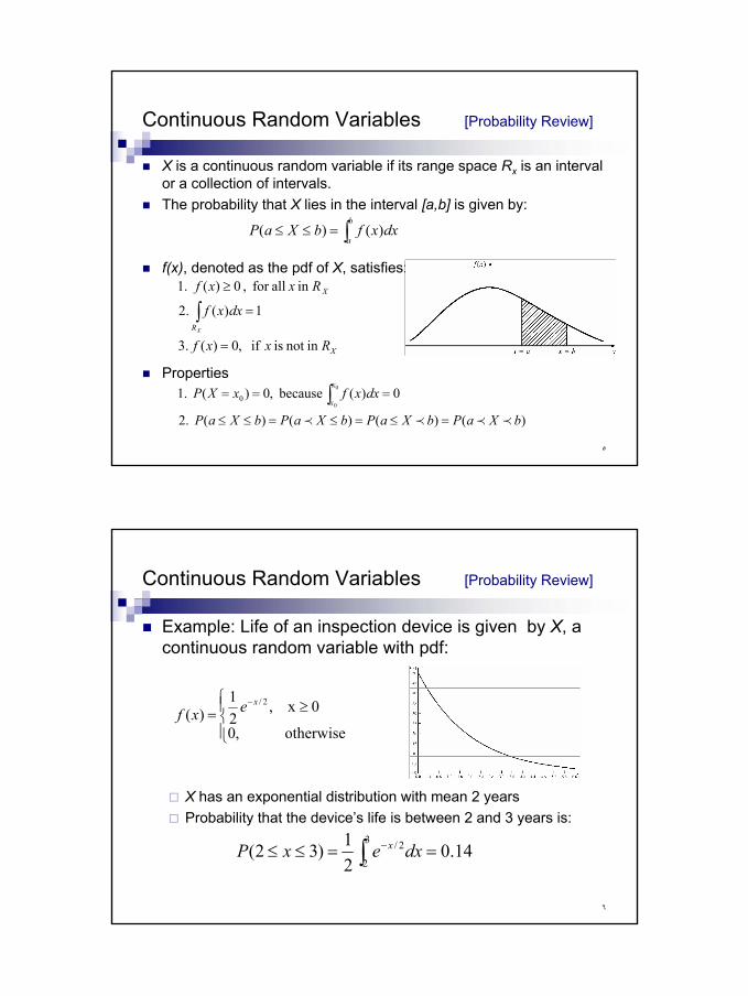
Example: Life of an inspection device is given by X, a continuous random variable with pdf:

X has an exponential distribution with mean 2 yearsProbability that the device’s life is between 2 and 3 years is:

≥=

−

otherwise ,0

0 x,21

)(2/xexf

14.021)32(

3

2

2/ ==≤≤ ∫ − dxexP x

٤

٧

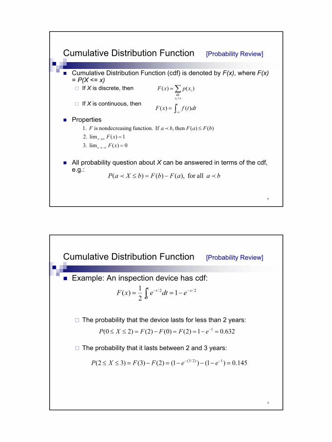
Cumulative Distribution Function [Probability Review]

Cumulative Distribution Function (cdf) is denoted by F(x), where F(x) = P(X <= x)

If X is discrete, then

If X is continuous, then

Properties

All probability question about X can be answered in terms of the cdf, e.g.:

∑≤

=

xx

i

i

xpxF all

)()(

∫ ∞−=

xdttfxF )()(

0)(lim 3.1)(lim 2.

)()( then , If function. ingnondecreas is 1.

==

≤

−∞→

∞→

xFxF

bFaFbaF

x

x

p

baaFbFbXaP pp allfor ,)()()( −=≤

٨

Cumulative Distribution Function [Probability Review]

Example: An inspection device has cdf:

The probability that the device lasts for less than 2 years:

The probability that it lasts between 2 and 3 years:

2/

0

2/ 121)( xx t edtexF −− −== ∫

632.01)2()0()2()20( 1 =−==−=≤≤ −eFFFXP

145.0)1()1()2()3()32( 1)2/3( =−−−=−=≤≤ −− eeFFXP

٥

٩

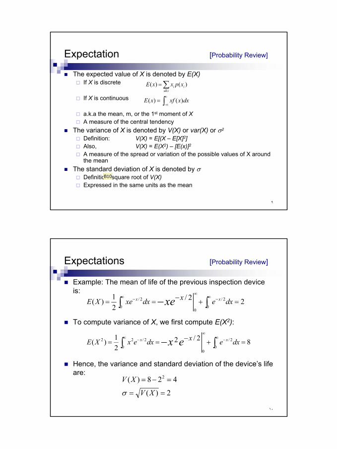
Expectation [Probability Review]

The expected value of X is denoted by E(X)If X is discrete

If X is continuous

a.k.a the mean, m, or the 1st moment of XA measure of the central tendency

The variance of X is denoted by V(X) or var(X) or σ2

Definition: V(X) = E[(X – E[X]2]Also, V(X) = E(X2) – [E(x)]2A measure of the spread or variation of the possible values of X around the mean

The standard deviation of X is denoted by σDefinition: square root of V(X)Expressed in the same units as the mean

∑=i

ii xpxxE all

)()(

∫∞

∞−= dxxxfxE )()(

B10

١٠

Expectations [Probability Review]

Example: The mean of life of the previous inspection device is:

To compute variance of X, we first compute E(X2):

Hence, the variance and standard deviation of the device’s life are:

22/21)(

0

2/

00

2/ =+−== ∫−∫∞ −

∞∞ − dxexdxxeXE xx xe

82/221)(

0

2/

00

2/22 =+−== ∫−∫∞ −

∞∞ − dxexdxexXE xx ex

2)(

428)( 2

==

=−=

XV

XV

σ

Slide 9

B10 after :, two spaces, then next word starts with a capital letterBrian; 2005/01/07

٦

١١

Useful Statistical Models

In this section, statistical models appropriate to some application areas are presented. The areas include:

Queueing systemsInventory and supply-chain systemsReliability and maintainabilityLimited data

١٢

Queueing Systems [Useful Models]

In a queueing system, interarrival and service-time patterns can be probablistic (for more queueing examples, see Chapter 2).

Sample statistical models for interarrival or service time distribution:

Exponential distribution: if service times are completely randomNormal distribution: fairly constant but with some random variability (either positive or negative)Truncated normal distribution: similar to normal distribution but with restricted value.Gamma and Weibull distribution: more general than exponential (involving location of the modes of pdf’s and the shapes of tails.)

٧

١٣

Inventory and supply chain [Useful Models]

In realistic inventory and supply-chain systems, there are at least three random variables:

The number of units demanded per order or per time periodThe time between demandsThe lead time

Sample statistical models for lead time distribution:Gamma

Sample statistical models for demand distribution: Poisson: simple and extensively tabulated.Negative binomial distribution: longer tail than Poisson (more large demands).Geometric: special case of negative binomial given at least one demand has occurred.

١٤

Reliability and maintainability [Useful Models]

Time to failure (TTF)Exponential: failures are randomGamma: for standby redundancy where each component has an exponential TTFWeibull: failure is due to the most serious of a large number of defects in a system of componentsNormal: failures are due to wear

٨

١٥

Other areas [Useful Models]

For cases with limited data, some useful distributions are:

Uniform, triangular and beta Other distribution: Bernoulli, binomial and hyperexponential.

١٦

Discrete Distributions

Discrete random variables are used to describe random phenomena in which only integer values can occur.In this section, we will learn about:

Bernoulli trials and Bernoulli distributionBinomial distributionGeometric and negative binomial distributionPoisson distribution

٩

١٧

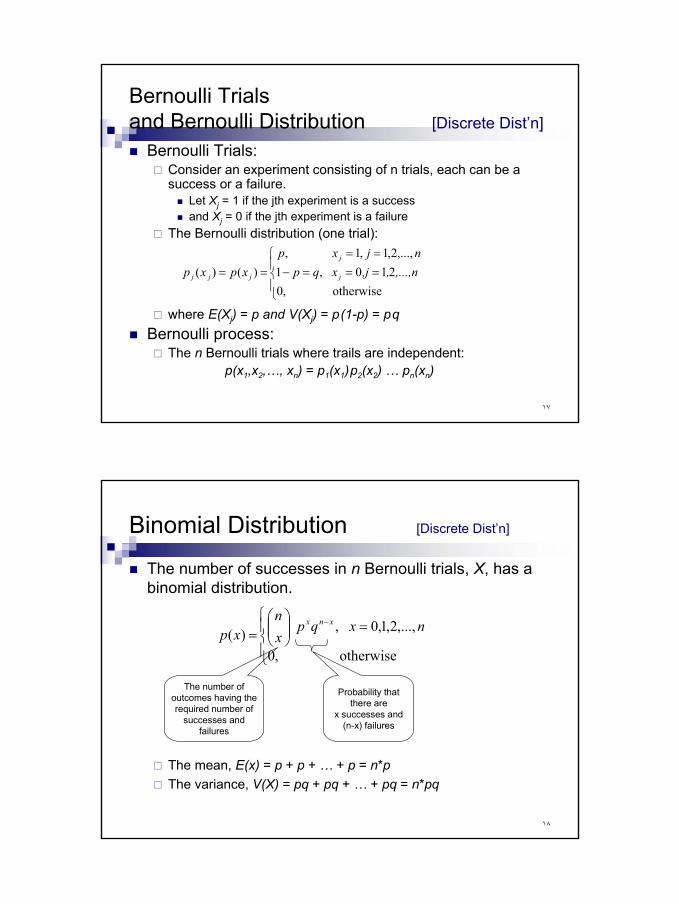
Bernoulli Trials and Bernoulli Distribution [Discrete Dist’n]

Bernoulli Trials: Consider an experiment consisting of n trials, each can be a success or a failure.

Let Xj = 1 if the jth experiment is a successand Xj = 0 if the jth experiment is a failure

The Bernoulli distribution (one trial):

where E(Xj) = p and V(Xj) = p(1-p) = pqBernoulli process:

The n Bernoulli trials where trails are independent:p(x1,x2,…, xn) = p1(x1)p2(x2) … pn(xn)

===−==

==otherwise ,0

210 ,1,...,2,1,1 ,

)()( ,...,n,,jxqpnjxp

xpxp j

j

jjj

١٨

Binomial Distribution [Discrete Dist’n]

The number of successes in n Bernoulli trials, X, has a binomial distribution.

The mean, E(x) = p + p + … + p = n*pThe variance, V(X) = pq + pq + … + pq = n*pq

The number of outcomes having the required number of

successes and failures

Probability that there are

x successes and (n-x) failures

=

=

−

otherwise ,0

,...,2,1,0 , )( nxqpxn

xpxnx

١٠

١٩

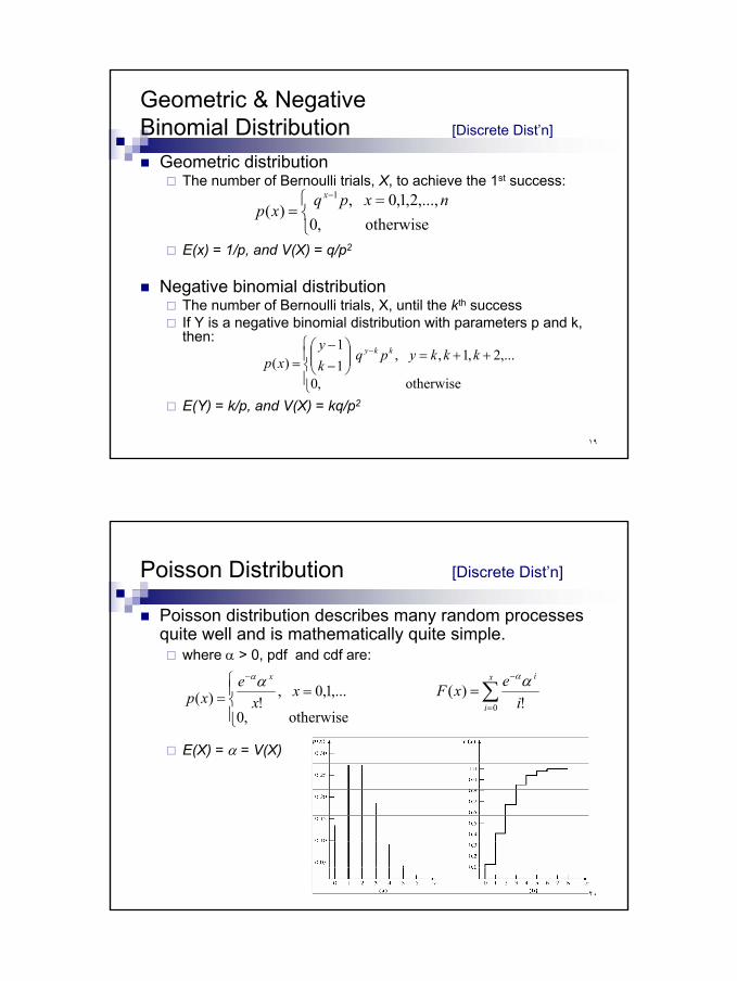
Geometric & NegativeBinomial Distribution [Discrete Dist’n]

Geometric distributionThe number of Bernoulli trials, X, to achieve the 1st success:

E(x) = 1/p, and V(X) = q/p2

Negative binomial distributionThe number of Bernoulli trials, X, until the kth success If Y is a negative binomial distribution with parameters p and k, then:

E(Y) = k/p, and V(X) = kq/p2

=

=−

otherwise ,0,...,2,1,0 ,

)(1 nxpq

xpx

++=

−−

=−

otherwise ,0

,...2,1, , 11

)( kkkypqky

xpkky

٢٠

Poisson Distribution [Discrete Dist’n]

Poisson distribution describes many random processes quite well and is mathematically quite simple.

where α > 0, pdf and cdf are:

E(X) = α = V(X)

==

−

otherwise ,0

,...1,0 ,!)( xx

exp

xαα

∑=

−

=x

i

i

iexF

0 !)( αα

١١

٢١

Poisson Distribution [Discrete Dist’n]

Example: A computer repair person is “beeped” each time there is a call for service. The number of beeps per hour ~ Poisson(α = 2 per hour).

The probability of three beeps in the next hour:p(3) = e-223/3! = 0.18

also, p(3) = F(3) – F(2) = 0.857-0.677=0.18

The probability of two or more beeps in a 1-hour period:p(2 or more) = 1 – p(0) – p(1)

= 1 – F(1) = 0.594

٢٢

Continuous Distributions

Continuous random variables can be used to describe random phenomena in which the variable can take on any value in some interval.In this section, the distributions studied are:

UniformExponentialNormalWeibullLognormal

١٢

٢٣

Uniform Distribution [Continuous Dist’n]

A random variable X is uniformly distributed on the interval (a,b), U(a,b), if its pdf and cdf are:

PropertiesP(x1 < X < x2) is proportional to the length of the interval [F(x2) –F(x1) = (x2-x1)/(b-a)]E(X) = (a+b)/2 V(X) = (b-a)2/12

U(0,1) provides the means to generate random numbers, from which random variates can be generated.

≤≤

−=otherwise ,0

,1)( bxa

abxf

≥

≤−−

=

bx

bxaabax

ax

xF

,1

,

,0

)( p

p

٢٤

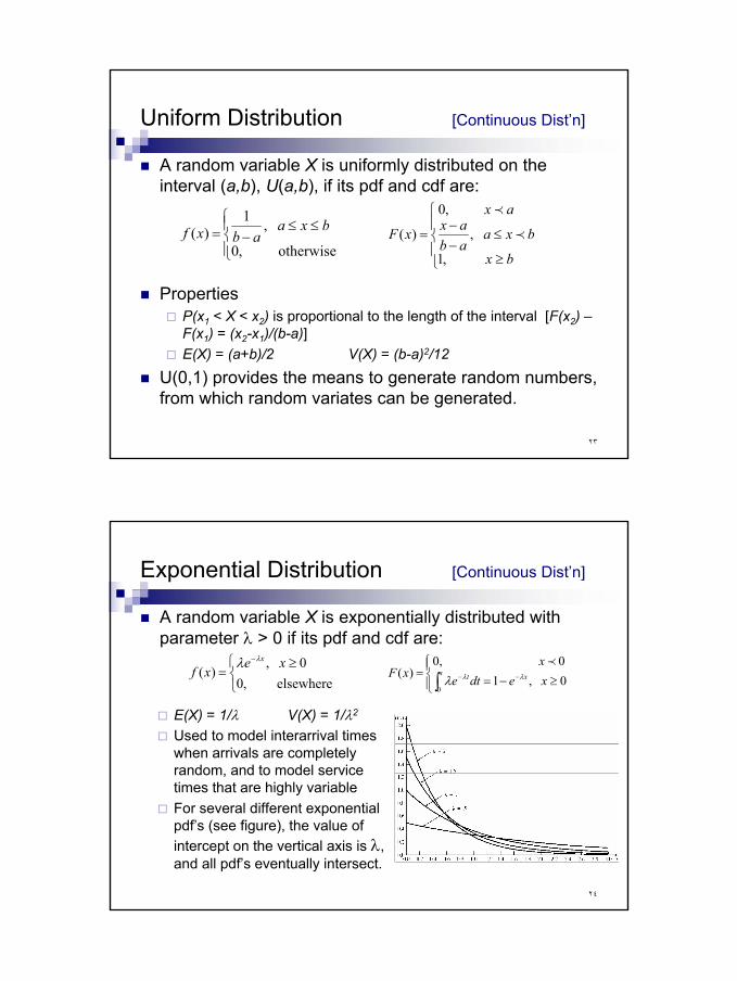
Exponential Distribution [Continuous Dist’n]

A random variable X is exponentially distributed with parameter λ > 0 if its pdf and cdf are:

≥

=−

elsewhere ,00 ,

)(xe

xfxλλ

≥−==

∫ −− 0 ,10 0,

)(0

xedtex

xF x xt λλλp

E(X) = 1/λ V(X) = 1/λ2

Used to model interarrival times when arrivals are completely random, and to model service times that are highly variableFor several different exponential pdf’s (see figure), the value of intercept on the vertical axis is λ, and all pdf’s eventually intersect.

١٣

٢٥

Exponential Distribution [Continuous Dist’n]

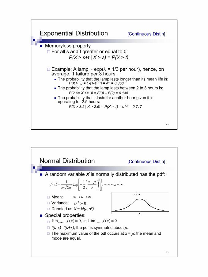
Memoryless propertyFor all s and t greater or equal to 0:

P(X > s+t | X > s) = P(X > t)

Example: A lamp ~ exp(λ = 1/3 per hour), hence, on average, 1 failure per 3 hours.

The probability that the lamp lasts longer than its mean life is:P(X > 3) = 1-(1-e-3/3) = e-1 = 0.368

The probability that the lamp lasts between 2 to 3 hours is:P(2 <= X <= 3) = F(3) – F(2) = 0.145

The probability that it lasts for another hour given it is operating for 2.5 hours:

P(X > 3.5 | X > 2.5) = P(X > 1) = e-1/3 = 0.717

٢٦

Normal Distribution [Continuous Dist’n]

A random variable X is normally distributed has the pdf:

Mean:Variance:Denoted as X ~ N(µ,σ2)

Special properties:.

f(µ-x)=f(µ+x); the pdf is symmetric about µ.The maximum value of the pdf occurs at x = µ; the mean and mode are equal.

0)(lim and ,0)(lim == ∞→−∞→ xfxf xx

∞∞−

−

−= pp xxxf ,21exp

21)(

2

σµ

πσ

∞∞− pp µ02 fσ

١٤

٢٧

Normal Distribution [Continuous Dist’n]

Evaluating the distribution:Use numerical methods (no closed form)Independent of µ and σ, using the standard normal distribution:

Z ~ N(0,1)Transformation of variables: let Z = (X - µ) / σ,

∫ ∞−

−=Φz t dtez 2/2

21)( where,π

( )

)()(

21

)(

/)(

/)( 2/2

σµσµ

σµ

φ

π

σµ

−−

∞−

−

∞−

−

Φ==

=

−

≤=≤=

∫

∫xx

x z

dzz

dze

xZPxXPxF

٢٨

Normal Distribution [Continuous Dist’n]

Example: The time required to load an oceangoing vessel, X, is distributed as N(12,4)

The probability that the vessel is loaded in less than 10 hours:

Using the symmetry property, Φ(1) is the complement of Φ (-1)

1587.0)1(2

1210)10( =−Φ=

−

Φ=F

١٥

٢٩

Weibull Distribution [Continuous Dist’n]

A random variable X has a Weibull distribution if its pdf has the form:

3 parameters:Location parameter: υ, Scale parameter: β , (β > 0)Shape parameter. α, (> 0)

Example: υ = 0 and α = 1:

≥

−

−

−

=

−

otherwise ,0

,exp)(

1

να

να

ναβ ββ

xxxxf

)( ∞−∞ ppν

When β = 1, X ~ exp(λ = 1/α)

٣٠

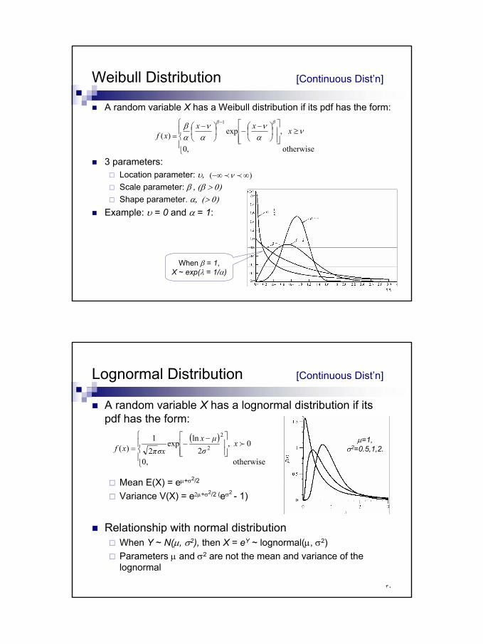
Lognormal Distribution [Continuous Dist’n]

A random variable X has a lognormal distribution if its pdf has the form:

Mean E(X) = eµ+σ2/2

Variance V(X) = e2µ+σ2/2 (eσ2 - 1)

Relationship with normal distributionWhen Y ~ N(µ, σ2), then X = eY ~ lognormal(µ, σ2)Parameters µ and σ2 are not the mean and variance of the lognormal

( )

−−=

otherwise 0,

0 ,2

lnexp21

)(

2

2 fxσµx

σxπxfµ=1,

σ2=0.5,1,2.

١٦

٣١

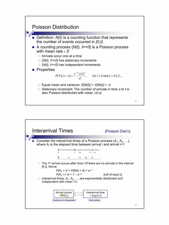
Poisson Distribution

Definition: N(t) is a counting function that represents the number of events occurred in [0,t].A counting process {N(t), t>=0} is a Poisson process with mean rate λ if:

Arrivals occur one at a time{N(t), t>=0} has stationary increments{N(t), t>=0} has independent increments

Properties

Equal mean and variance: E[N(t)] = V[N(t)] = λtStationary increment: The number of arrivals in time s to t is also Poisson-distributed with mean λ(t-s)

,...2,1,0 and 0for ,!

)(])([ =≥==−

ntntentNPnt λλ

٣٢

Stationary & Independent Memoryless

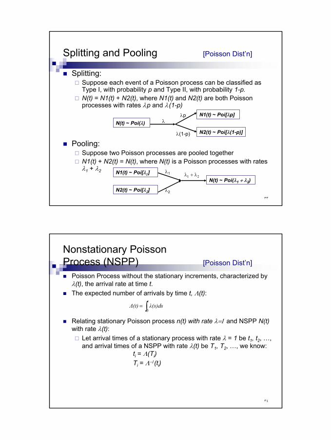
Interarrival Times [Poisson Dist’n]

Consider the interarrival times of a Possion process (A1, A2, …), where Ai is the elapsed time between arrival i and arrival i+1

The 1st arrival occurs after time t iff there are no arrivals in the interval [0,t], hence:

P{A1 > t} = P{N(t) = 0} = e-λt

P{A1 <= t} = 1 – e-λt [cdf of exp(λ)]Interarrival times, A1, A2, …, are exponentially distributed and independent with mean 1/λ

Arrival counts ~ Poi(λ)

Interarrival time ~ Exp(1/λ)B42

Slide 32

B42 Poi is not an abbreviation of Poisson that I have ever seenBrian; 2005/01/07

١٧

٣٣

Splitting and Pooling [Poisson Dist’n]

Splitting:Suppose each event of a Poisson process can be classified as Type I, with probability p and Type II, with probability 1-p.N(t) = N1(t) + N2(t), where N1(t) and N2(t) are both Poisson processes with rates λp and λ(1-p)

Pooling:Suppose two Poisson processes are pooled togetherN1(t) + N2(t) = N(t), where N(t) is a Poisson processes with rates λ1 + λ2

N(t) ~ Poi(λ)N1(t) ~ Poi[λp]

N2(t) ~ Poi[λ(1-p)]

λλp

λ(1-p)

N(t) ~ Poi(λ1 + λ2)N1(t) ~ Poi[λ1]

N2(t) ~ Poi[λ2]

λ1 + λ2λ1

λ2

٣٤

Nonstationary Poisson Process (NSPP) [Poisson Dist’n]

Poisson Process without the stationary increments, characterized by λ(t), the arrival rate at time t.The expected number of arrivals by time t, Λ(t):

Relating stationary Poisson process n(t) with rate λ=1 and NSPP N(t)with rate λ(t):

Let arrival times of a stationary process with rate λ = 1 be t1, t2, …, and arrival times of a NSPP with rate λ(t) be T1, T2, …, we know:

ti = Λ(Ti)Ti = Λ−1(ti)

∫=tλ(s)dsΛ(t)

0

١٨

٣٥

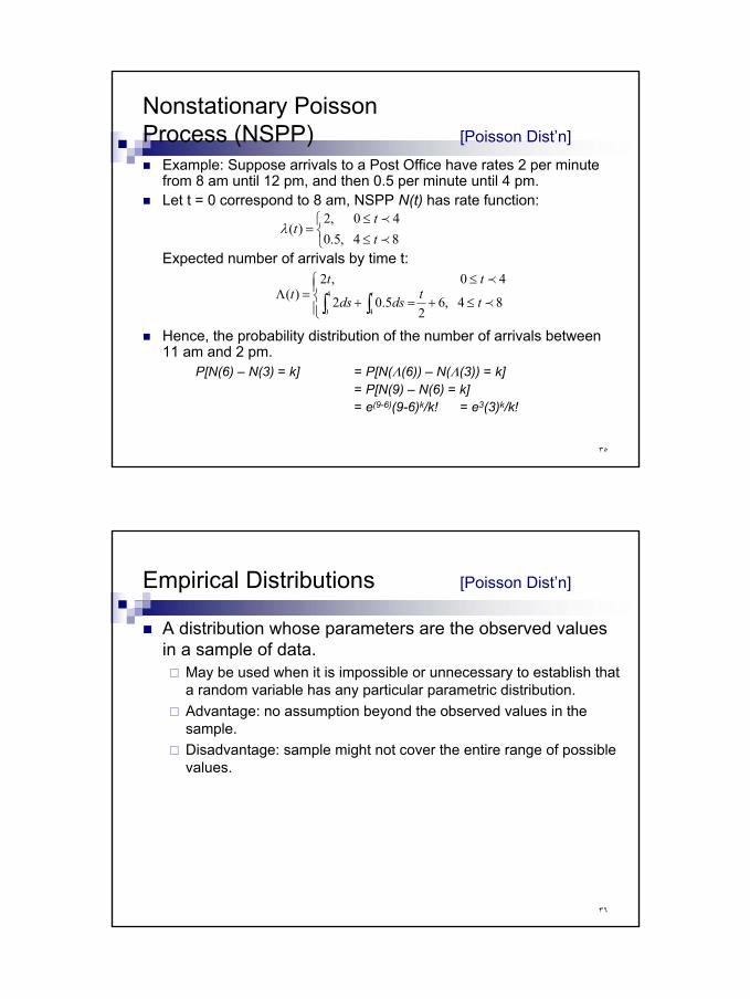
Example: Suppose arrivals to a Post Office have rates 2 per minute from 8 am until 12 pm, and then 0.5 per minute until 4 pm. Let t = 0 correspond to 8 am, NSPP N(t) has rate function:

Expected number of arrivals by time t:

Hence, the probability distribution of the number of arrivals between 11 am and 2 pm.

P[N(6) – N(3) = k] = P[N(Λ(6)) – N(Λ(3)) = k]= P[N(9) – N(6) = k]= e(9-6)(9-6)k/k! = e3(3)k/k!

≤≤

=84 ,5.040 ,2

)(p

p

tt

tλ

≤+=+

≤=Λ

∫ ∫ 84 ,62

5.02

40 ,2)( 4

0 4p

p

ttdsds

ttt t

Nonstationary Poisson Process (NSPP) [Poisson Dist’n]

٣٦

A distribution whose parameters are the observed values in a sample of data.

May be used when it is impossible or unnecessary to establish that a random variable has any particular parametric distribution.Advantage: no assumption beyond the observed values in the sample.Disadvantage: sample might not cover the entire range of possible values.

Empirical Distributions [Poisson Dist’n]

١٩

٣٧

The world that the simulation analyst sees is probabilistic, not deterministic.In this chapter:

Reviewed several important probability distributions.Showed applications of the probability distributions in a simulation context.

Important task in simulation modeling is the collection and analysis of input data, e.g., hypothesize a distributional form for the input data. Reader should know:

Difference between discrete, continuous, and empirical distributions.Poisson process and its properties.

Summary