Assessment of regional climate model simulation … of regional climate model simulation estimates ... climate model simulation estimates over ... or statistical methods. Statistical

Assessment of regional climate model simulation estimatesover the northeast United States

M. A. Rawlins,1 R. S. Bradley,1 and H. F. Diaz2

Received 18 May 2012; revised 19 October 2012; accepted 22 October 2012; published 12 December 2012.

[1] Given the coarse scales of coupled atmosphere-ocean global climate models, regionalclimate models (RCMs) are increasingly relied upon for studies at scales appropriate formany impacts studies. We use outputs from an ensemble of RCMs participating in theNorth American Regional Climate Change Assessment Program (NARCCAP) toinvestigate potential changes in seasonal air temperature and precipitation between present(1971–2000) and future (2041–2070) time periods across the northeast United States.The models show a consistent modest cold bias each season and are wetter thanobservations in winter, spring, and summer. Agreement in spatial variability and patterncorrelation is good for air temperature and marginal for precipitation. Two methods wereused to evaluate robustness of the mid 21st century change projections; one whichestimates model reliability to generate multimodel means and assess uncertainty and asecond which depicts multimodel projections by separating lack of climate change signalfrom lack of model agreement. For air temperature we find changes of 2–3�C are outsidethe level of internal natural variability and significant at all northeast grid cells. Signals ofprecipitation increases in winter are significant region wide. Regionally averagedprecipitation changes for spring, summer, and autumn are within the level of naturalvariability. This study raises confidence in mid 21st century temperature projectionsacross the northeast United States and illustrates the value in comprehensive assessmentsof regional climate model projections over time and space scales where natural variabilitymay obscure signals of anthropogenically forced changes.

Citation: Rawlins, M. A., R. S. Bradley, and H. F. Diaz (2012), Assessment of regional climate model simulation estimates overthe northeast United States, J. Geophys. Res., 117, D23112, doi:10.1029/2012JD018137.

1. Introduction

[2] Current trajectories in greenhouse gas concentrationsare increasing the likelihood of significant impacts fromclimate change in coming decades. A recent study using amultithousand-member perturbed-physics ensemble showedglobal-mean temperature increases of 1.4 to 3 K by 2050,relative to 1961–1990 under a mid-range forcing scenario[Rowlands et al., 2012]. However, the geographic pattern ofchange is not uniform. Understanding both the magnitudeand uncertainty in climate change projections at the regionalscale is critical, as uncertainties in the regional climateresponse can lead to uncertainties in associated climateimpacts [Mearns, 2003; Wood et al., 2004].[3] Model simulations suggest the potential for future

temperature and precipitation changes across the northeast

United States. By the end of the 21st century, warming can beexpected across all seasons, and winter precipitation is pro-jected to increase by 11 to 14% depending on the emissionscenario used in the simulations [Hayhoe et al., 2007]. Cli-mate change studies have traditionally been performed usingatmosphere-ocean general circulation models (AOGCMs)with resolutions of 100 to 400 km [Alley et al., 2007]. Thesecoarse scales leave AOGCMs unable to capture the effects oflocal forcings such as complex topography which modulatesthe models’ climate signal at local scales. To overcome thisshortcoming, downscaling of climate model simulations hasbecome common and has been shown to provide valuableinformation for impacts research and adaptation planning[Mearns et al., 2009; Wood et al., 2004]. Downscaling canbe achieved through either dynamical or statistical methods.Statistical downscaling typically involves relating largescale climate features to local climate at a particular loca-tion. Dynamical downscaling involves the application of aregional climate model (RCM) forced by global climatemodel boundary conditions. More realistic parameteriza-tions of surface processes in sophisticated RCM land-sur-face schemes can provide more realistic simulations ofsurface conditions and the associated physical processescritical to the simulation of climate extremes [Roy et al.,2011]. Large international efforts such as PRUDENCE

1Climate System Research Center, Department of Geosciences,University of Massachusetts, Amherst, Massachusetts, USA.

2Climate Diagnostics Center, Office of Atmospheric Research, NationalOceanic and Atmospheric Administration, Boulder, Colorado, USA.

Corresponding author: M. A. Rawlins, Climate System Research Center,Department of Geosciences, University of Massachusetts, 611 NorthPleasant St., Amherst, MA 01002, USA. ([email protected])

©2012. American Geophysical Union. All Rights Reserved.0148-0227/12/2012JD018137

JOURNAL OF GEOPHYSICAL RESEARCH, VOL. 117, D23112, doi:10.1029/2012JD018137, 2012

D23112 1 of 15

(http://prudence.dmi.dk/), ENSEMBLES (http://ensembles-eu.metoffice.com/), and CORDEX have made use of highresolution downscaled model data for projections of futureclimates at regional scales [Giorgi et al., 2009].[4] The North American Regional Climate Change

Assessment Program (NARCCAP) [Mearns et al., 2007] isproducing high resolution climate change simulations fromdifferent combinations of AOGCMs and RCMs, providing arich set of data that facilitate investigations of uncertainties inregional scale projections of future climate across NorthAmerica [Mearns et al., 2009].Mearns et al. [2012] describeresults from Phase I, an evaluation component of the pro-gram, wherein the RCMs are nested within NCEP/DOEglobal reanalysis II. Their comparisons with observed datafor the period 1980–2004 show that, for air temperatureacross North America, both positive (model overestimates)and negative biases occur. The Hadley Regional ClimateModel 3 (HRM3) exhibits a large warm bias in winter andsummer. Both positive and negative biases are noted withsummer precipitation. For winter, precipitation biases arelargely positive. Phase I results showed relatively low tem-perature and precipitation biases over the northeast. TheRCMs replicate well the monthly frequency of precipitationextremes across coastal California, where the precipitation islargely topographic, while performing somewhat less wellacross the UpperMississippi River watershed [Gutowski et al.,2010]. NARCCAP data have been used to characterizepotential future increases in the intensity of extreme winterprecipitation across the western United States [Dominguezet al., 2012] and to produce projections of seasonal climateacross the southeast United States [Sobolowski and Pavelsky,2012]. Simulations with the Abdus Salam Institute Theoreti-cal Physics Regional Climate Model Version 3 (RegCM3),one of models used by NARCCAP, suggest an increased fre-quency of extreme hot events and a decreased frequency ofextreme cold events across much of the northeast, by latecentury [Diffenbaugh et al., 2005]. This RCM also simulated afuture increases in mean annual and extreme precipitationevent frequency. NARCCAP RCM simulations and data fromeach respective driving GCM were used to construct proba-bilistic projections of high-resolution monthly temperatureover North America [Li et al., 2012].[5] Detailed assessments of individual model errors, often

termed ‘biases’, are critical to determining model usefulnessfor understanding potential impacts of climate change. Theability to simulate the climate of a region depends largely onthe quality of the forcing AOGCM and the degree to which itrepresents flow conditions at the boundary [Christensenet al., 1998; Giorgi et al., 2001]. For example, biases ofonly a few models can affect the multimodel mean and resultin physically unrealistic results. One analysis [Liepert andPrevidi, 2012] found that many of the studied AOGCMshad an unphysical and hence ‘ghost’ sink or source ofatmospheric moisture. Several recent studies shed light onthe nature of uncertainty in climate change projections. Forinstance, Hawkins and Sutton [2011] in an analysis of theCMIP3 multimodel ensemble found that for decadal meansof seasonal mean precipitation, internal variability is thedominant uncertainty for predictions of the first decadeeverywhere, and for many regions until the third decadeahead. Model uncertainty is generally the dominant sourceof uncertainty for longer lead times. In an earlier review

[Hawkins and Sutton, 2009] showed how the differentcontributions to climate projection uncertainty vary withlead-time over the 21st century (see their Figures 2 and 3).Beyond about 20 years, model uncertainty becomes greaterthan internal variability, and of course, emission scenariouncertainty becomes dominant after about mid-century. Mostrecently, Deser et al. [2012] found that the dominant sourceof uncertainty in the simulated climate response using a40-member simulation ensemble with the NCAR Commu-nity Climate System Model Version 3 (CCSM3) under theSRES A1B for middle and high latitudes is internal atmo-spheric variability, and that uncertainties in the forcedresponse are generally larger for sea level pressure than pre-cipitation, and smallest for air temperature. Thus the impli-cation from that study is that forced changes in airtemperature can be detected earlier and with fewer ensemblemembers than those in atmospheric circulation and precipi-tation. The availability of multimodel simulations has helpedto focus efforts on new approaches to synthesize climatechange projections [Giorgi and Mearns, 2002; Knutti et al.,2010; Tebaldi and Knutti, 2007; Tebaldi et al., 2011]. Thisincludes methods which weight models based on perfor-mance relative to present-day conditions and/or the deviationfrom the group mean [Giorgi and Mearns, 2002, 2003].Christensen et al. [2010] describe a weighting scheme whichincorporates six model performance metrics. Tebaldi et al.[2011] argue that assessments using multiple climate mod-els should separate lack of climate change signal from lack ofmodel agreement by assessing the degree of consensus on thesignificance of the change as well as the sign of the change.[6] In this study we describe the sign, magnitude, and

quantitative significance of precipitation and temperaturechanges across the northeast United States between theperiods 2041–2070 and 1971–2000. We apply a methoddesigned for calculating average, uncertainty range, and ameasure of reliability of simulated climate changes at theregional scale from ensembles of different climate modelsimulations. A second method, which complements the first,is used to account for model performance and natural vari-ability and, in turn, determine best estimates of likelychanges by mid-century. The climate change analysis fol-lows an assessment of model performance relative to fieldsderived from observed station data. Investigating the abilityof the suite of RCMs to capture the magnitude and vari-ability in current climate provides additional information ontheir potential for improving understanding of regional scaleclimate change impacts across the northeast United States.

2. Data and Methods

2.1. Model Data

[7] The NARCCAP [Mearns et al., 2007] is archivingoutputs from a set of regional climate model (RCM) simu-lations over a domain spanning North America. For theNARCCAP effort, each participating RCM is forced withboundary conditions from at least two atmosphere-oceangeneral circulation models (AOGCMs). Table 1 list themodels and the respective modeling centers. Three hourlyRCM outputs are available for the contemporary period1971–2000 and for the future period 2041–2070. TheNARCCAP effort involves the use of the SRES A2 emis-sions scenario [Nakicenovic et al., 2000] by all modeling

RAWLINS ET AL.: NORTHEAST CLIMATE CHANGES FROM RCMS D23112D23112

2 of 15

groups. Use of the high mid-century greenhouse gas con-centrations of the A2 scenario may not be unreasonable givenrecent greenhouse gas concentration trajectories (P. Tan andR. Keeling, Trends in atmospheric carbon dioxide, 2012,Scripps Institution of Oceanography (scrippsco2.ucsd.edu/))and the fact that the commonly used A1B scenario closelytracks A2 through mid century. We use 2 m air temperaturesand precipitation data for a subset of GCM-RCM pairsavailable at the time of this writing. Table 2 shows the cur-rently available model pairs among all planned NARCCAPcombinations. When discussing a model simulation weuse the convention GCM_RCM, for example CCSM_MM5.Spatial resolution for each model is approximately 50 km andeach RCM has its own native grid. For this study we derivedseasonal means and totals from the archived 3 hourly data.To facilitate the analysis we interpolated all native data valuesto a common 0.5 degree grid. Our analysis includes all0.5 degree grid cells which fall within the 9 northeast U.S.states. A more complete discussion of the NARCCAP projectis presented in Mearns et al. [2009].

2.2. Observed Data

[8] Bias assessments were made by comparing estimatesfrom NARCCAP GCM-RCM pairings with data representingair temperature and precipitation observations from stationrecords. We use monthly 2 m air temperatures and precipi-tation on a 0.5 degree grid available from the University ofDelaware (UDel) database (K. Matsuura and C. J. Willmott,Terrestrial air temperature: 1900–2008 gridded monthly timeseries, version 2.01, 2009, http://climate.geog.udel.edu/�climate/; C. J. Willmott and K. Matsuura, Terrestrial precip-itation: 1900–2008 gridded monthly time series, version 2.01,2009, http://climate.geog.udel.edu/�climate/). The UDel dataset was developed through interpolations of meteorologicalstation data which account for the lapse rate in temperaturewith increasing elevation [Willmott and Matsuura, 1995] andmakes use of spatially high-resolution air temperature andprecipitation climatologies [Willmott and Robeson, 1995].Monthly values over the period 1971–2000 are used here to

construct fields of seasonal mean air temperatures and pre-cipitation at each grid cell over the northeast.

2.3. Analysis

[9] This paper presents an assessment of biases anduncertainties in seasonal air temperatures and precipitationfields among the available NARCCAP GCM-RCM pairs.We focus on mean climate across the northeast United Statesfor each season over the two periods, hereafter the “present”(1971–2000) and “future” (2041–2070). Seasons are definedusing monthly values as follows: winter (DJF), spring(MAM), summer (JJA), and autumn (SON). Through thisanalysis we quantify regional averages from the models andobservations and describe changes in the projected meanseasonal climate. We also examine biases between RCM andobserved data fields and changes in statistical properties ofthe fields.[10] Uncertainties in future climate projections can be

estimated through use of not only multimodel ensembles,but also through application of statistical methods whichtake into account the natural climate variability (�) and theperformance of individual models in relation to the ensemblegroup. To improve our assessments we apply here the reli-ability ensemble averaging (REA) method [Giorgi andMearns, 2002] to determine average, uncertainty range, anda measure of reliability of simulated changes from theensemble of available NARCCAP GCM-RCM pairings.Sobolowski and Pavelsky [2012] applied the REA methodtogether with NARCCAP data to estimate likely future airtemperature and precipitation changes across the southeastUnited States.[11] The REA method defines a change over two time

periods as a weighted average of ensemble climate modelmembers. Here each climate model value is the regionallyaveraged seasonal temperature. Two model reliability factorscontribute to the weighting for each model; a factor based ona model’s ability to reproduce current climate and a factorbased on the distance of the model’s change estimate fromthe REA average. A simple multimodel mean of ensemblemembers for, as an example, season temperature T is

DT ¼ 1

N

Xi¼1;N

DTi ð1Þ

where N is the number of models, the overbar indicatesensemble averaging, and D indicates the simulated change.

Table 1. Models Used in This Study

Global Model Model Center

CCSM National Center for AtmosphericResearch

CGCM3.1 Canadian Centre for ClimateModeling and Analysis, Canada

GFDL Geophysical Fluid DynamicsLaboratory, USA

HadCM3 Hadley Centre for Climate Predictionand Research / Met Office, UK

Regional Model Model Center

CRCM OURANOS / UQAM, CanadaECP2 UC San Diego / Scripps Institute of

Oceanography, USAHRM3 Hadley Centre for Climate Prediction

and Research / Met Office, UKMM5 Iowa State University, USARCM3 UC Santa Cruz, USAWRFG Pacific Northwest National Lab, USA

Table 2. Regional Climate Model (RCM) and Forcing Atmosphere-Ocean General Circulation Model (AOGCM) Combinations Usedin This Studya

Global Models

Regional Models

CRCM ECP2 HRM3 MM5 RCM3 WRFG

CCSM 1 2 3CGCM3 4 5 6GFDL 7 X 8HADCM3 X 9 X

aWe use model pairings that have data for both historical and futureperiods. Numbers are references for model pairs examined. An ‘X’indicates a model pair for which data are being produced, but areunavailable at time of writing. See section 2.


3 of 15

With the REA method, the average change fDT is a weightedaverage of the ensemble members

fDT ¼ eA DTð Þ ¼X

iRiDTiXiRi

ð2Þ

where the operator eA indicates REA averaging and Ri is amodel reliability factor, defined

Ri ¼ RB;i

� �m � RD;i

� �n� � 1= m�nð Þ½ � ð3Þ

The factor RB,i is a measure representing model reliability asa function of model bias (BT,i) in simulating contemporarytemperature. The factor RD,i is a measure which reflectsmodel reliability in terms of the distance (DT,i) of the changecalculated by a given model from the REA average. Para-meters m and n are user defined weights for each reliabilityfactor. Here we choose a value of 1 for each weight. Theuncertainty range around the REA change is estimated usingthe root-mean square difference (rmsd) of the changes, ~dDT .The total uncertainty range is �~dDT or 2~dDT . Natural vari-ability, �T, for regionally averaged seasonal air temperature(�P for precipitation) is estimated using the UDel dataobserved fields. For temperature, the 100 year time series ofregionally averaged seasonal values is de-trended and thensmoothed using a 30 year running mean. The differencebetween the maximum and minimum values in the 100 yearsmoothed series becomes �T. Natural variability estimationand the other details of the REA method are described inGiorgi and Mearns [2002].[12] More recently, Tebaldi et al. [2011] introduced a

method appropriate for studies involving multiple models.The method separates lack of signal from lack of informa-tion due to model disagreement. It accomplishes this objec-tive by assessing the degree of consensus on the significanceof the change as well as the sign of the change. With thismethod, weather noise in the simulations is the variabilityover which significance in the model change signal is com-pared. Here, grids where at least 7 of the 9 models (X = 78%)show significant change and at least Y = 80% of thosemodels agree on sign of change are shaded by magnitudeand stippled. Grids are shaded by the multimodel mean butnot stippled where less than 7 of the models show significantchange. It is in these areas that Tebaldi et al. [2011] arguethat a signal of change lies within the noise of weather var-iability, and that the models still contain useful information.Areas where at least 7 of the models show significant changebut less than 80% of those model agree in sign are leftunshaded. For these grids the models are presentingconflicting information. Hence, confidence there is low. Theabove X and Y percentages are a subjective choice and canbe set differently based on the desired level of confidence.Our choices for X and Y are similar but not identical to the66% and 90% levels adopted in the Intergovernmental Panelon Climate Change’s Fourth Assessment Report [Alley et al.,2007]. We apply both techniques described by Giorgi andMearns [2002] and Tebaldi et al. [2011] to the NARCCAPmodel suite in order to answer questions regarding themagnitude and significance of projected climate changesacross the northeast United States. Narrowing down the

uncertainty range in climate model projections with the helpof observations is an important challenge in climate research[Mearns et al., 2012]. As Lenderink [2012] points out, while“it makes sense to weight model results according to themodel’s ability to represent pertinent aspects of the observedpresent-day climate … such an evaluation of simulations isfar from trivial”, and furthermore, while “… a model whosesimulations of the present-day climate are close to observa-tions [it] may well contain a set of errors that compensateeach other today, but may strongly distort the response toclimate warming as the balance between errors changes.”

3. Results and Discussion

3.1. Air Temperature

[13] The ability of models to reproduce contemporaryclimate is important, as large biases limit our confidence inprojections of future climate impacts such as extremeweather events. Regional climate models should capturewell the spatial variability in climatic fields along with theregionally averaged mean climate. For seasonal tempera-tures (1971–2000), the models as a group perform well incapturing spatial variability across the northeast UnitedStates as measured by standard deviation in the observed andmodel fields. Figure 1 shows Taylor diagrams which capturestatistics of the observed and model seasonal temperaturefield across the 211 northeast grid cells. The models tend toexhibit spatial variability which is similar to the observa-tional fields, as reflected by the agreement in standarddeviations. The models slightly underestimate spatial vari-ability in winter. Grid cell correlations are also relativelyhigh, generally greater than 0.85, and highest in winter.[14] Across the northeast United States, the NARCCAP

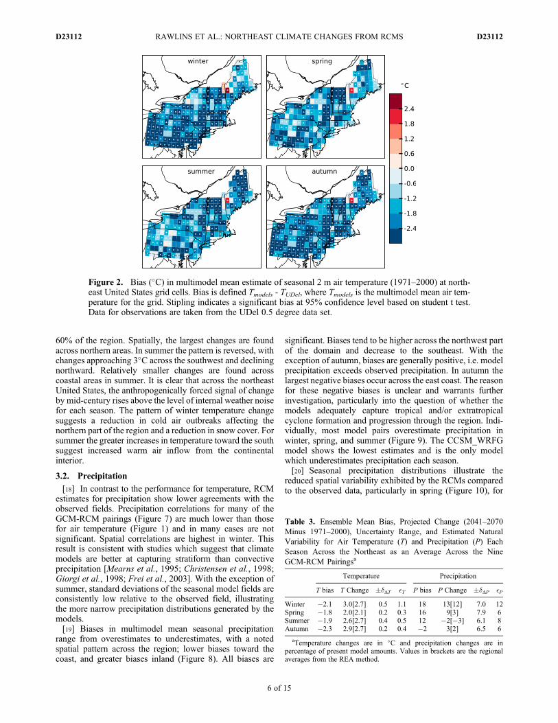
models tend to underestimate seasonal temperatures (Figure 2).No strong spatial pattern exists in the temperature bias fields.Biases are significant (95% confidence level based on studentt test) for 88, 62, 73, and 87% of the grid cells in winter,spring, summer, and autumn, respectively. The outlier overwestern Maine each season is a grid cell with a large amountof open water. An anomaly with the grid multimodel mean2 m temperature appears to be the source of the temperaturebias. Regional mean bias are �2.1, �1.8, �1.9, �2.3�C forwinter, spring, summer, autumn seasons, respectively(Table 3). Individually, all model pairings underestimatespatially averaged 1971–2000 mean temperature in summerand autumn (Figure 3). All but two model pairs(CCSM_MM5 and CGCM3_WRFG) underestimate tem-perature in winter, while all but two (CCSM_MM5 andCCSM_WRFG) underestimate it in spring.[15] Boxplots of seasonal air temperature distributions

for the gridded fields of present observations (O) andNARCCAP models present (P) and future (F) are shown inFigure 4. Comparing the distribution for the future periodalongside those for the present provides a sense of how pro-jected future changes compare with model biases. It alsoreveals if and how temperatures might change, along withother properties of the distribution. Temperature distributionsare nearly normal. In autumn, for example, while 25% of thegrid cells have observed temperature exceeding 10.9�C, noneof the RCM (multimodel mean) grid cells exceed that value.In summer a similarly shaped distribution is biased colder by


4 of 15

approximately 2�C. No change occurs with the shape oftemperature distributions between the present and futureperiods. Comparing the multimodel means for the presentand future periods shows seasonal temperature increases of3.0, 2.0, 2.6, 2.9�C in winter, spring, summer, and autumn,respectively (Figure 4). Thus, based on simple multimodelmeans for each season, the mean change exceeds the meanbias. The greater winter changes are consistent with expectedglobal trends assumed to be related to the ice-albedo feed-back [Dickinson et al., 1987; Hall, 2004]. A recent analysisof projected changes for the period 2035–2064 (relative to1961–1990) using nine AOGCMs and the A2 scenario[Hayhoe et al., 2007], however, found lower change magni-tudes across the northeast and, interestingly, a larger pro-jected increase in summer than winter. The study authorsspeculated that the larger change in summer versus winterwas attributable to feedbacks between evaporation and tem-perature along with a declining effect from the ice-albedofeedback.

[16] Applying the REAmethod [Giorgi andMearns, 2002]provides additional information regarding uncertainties inthe magnitude of future seasonal temperature changes(Figure 5). First, each REA average change differs from theensemble average change by a few tenths of a degree C, withwinter temperature changes across the northeast lower by0.3�C (2.7 versus 3.0�C). In comparison, natural variability(�T) is 0.5�C or less in spring, summer, and autumn, andapproximately 1�C in winter (Table 3). Thus, the magnitudeof change each season is well outside the range of naturalvariability. The uncertainty range calculated from the REAmethod (�dDT) is largest in winter and smallest in spring(Table 3).[17] Results from the model agreement mapping method

[Tebaldi et al., 2011] reveal interesting differences across theregion. Temperature changes are significant (95% level) overthe entire region in each season (Figure 6). As noted above,the ensemble mean change is largest in winter, where theprojected temperature increase exceeds 3�C across more than

Figure 1. Taylor diagrams showing standard deviation (�C), RMSE (�C), and correlation for theobserved and for each model seasonal (1971–2000) air temperature field across the northeast UnitedStates. Seasons throughout the analysis and in the subsequent figures are define winter (DJF); spring(MAM); summer (JJA); autumn (SON). GCMs and RCMs are listed in Table 1 and Table 2. Statisticsare calculated over all 211 grid cells of the observed field and from the nine GCM-RCM fields. The starindicates the statistics for the observed field. Contour of the reference standard deviation (from observedfield) is show by the dashed line. RMSE contours are in gray. Correlation rays are the (left) 95th and(right) 99th significance levels.


5 of 15

60% of the region. Spatially, the largest changes are foundacross northern areas. In summer the pattern is reversed, withchanges approaching 3�C across the southwest and decliningnorthward. Relatively smaller changes are found acrosscoastal areas in summer. It is clear that across the northeastUnited States, the anthropogenically forced signal of changeby mid-century rises above the level of internal weather noisefor each season. The pattern of winter temperature changesuggests a reduction in cold air outbreaks affecting thenorthern part of the region and a reduction in snow cover. Forsummer the greater increases in temperature toward the southsuggest increased warm air inflow from the continentalinterior.

3.2. Precipitation

[18] In contrast to the performance for temperature, RCMestimates for precipitation show lower agreements with theobserved fields. Precipitation correlations for many of theGCM-RCM pairings (Figure 7) are much lower than thosefor air temperature (Figure 1) and in many cases are notsignificant. Spatial correlations are highest in winter. Thisresult is consistent with studies which suggest that climatemodels are better at capturing stratiform than convectiveprecipitation [Mearns et al., 1995; Christensen et al., 1998;Giorgi et al., 1998; Frei et al., 2003]. With the exception ofsummer, standard deviations of the seasonal model fields areconsistently low relative to the observed field, illustratingthe more narrow precipitation distributions generated by themodels.[19] Biases in multimodel mean seasonal precipitation

range from overestimates to underestimates, with a notedspatial pattern across the region; lower biases toward thecoast, and greater biases inland (Figure 8). All biases are

significant. Biases tend to be higher across the northwest partof the domain and decrease to the southeast. With theexception of autumn, biases are generally positive, i.e. modelprecipitation exceeds observed precipitation. In autumn thelargest negative biases occur across the east coast. The reasonfor these negative biases is unclear and warrants furtherinvestigation, particularly into the question of whether themodels adequately capture tropical and/or extratropicalcyclone formation and progression through the region. Indi-vidually, most model pairs overestimate precipitation inwinter, spring, and summer (Figure 9). The CCSM_WRFGmodel shows the lowest estimates and is the only modelwhich underestimates precipitation each season.[20] Seasonal precipitation distributions illustrate the

reduced spatial variability exhibited by the RCMs comparedto the observed data, particularly in spring (Figure 10), for

Figure 2. Bias (�C) in multimodel mean estimate of seasonal 2 m air temperature (1971–2000) at north-east United States grid cells. Bias is defined Tmodels - TUDel, where Tmodels is the multimodel mean air tem-perature for the grid. Stipling indicates a significant bias at 95% confidence level based on student t test.Data for observations are taken from the UDel 0.5 degree data set.

Table 3. Ensemble Mean Bias, Projected Change (2041–2070Minus 1971–2000), Uncertainty Range, and Estimated NaturalVariability for Air Temperature (T) and Precipitation (P) EachSeason Across the Northeast as an Average Across the NineGCM-RCM Pairingsa

Temperature Precipitation

T bias T Change �dΔT �T P bias P Change �dΔP �P

Winter �2.1 3.0[2.7] 0.5 1.1 18 13[12] 7.0 12Spring �1.8 2.0[2.1] 0.2 0.3 16 9[3] 7.9 6Summer �1.9 2.6[2.7] 0.4 0.5 12 �2[�3] 6.1 8Autumn �2.3 2.9[2.7] 0.2 0.4 �2 3[2] 6.5 6

aTemperature changes are in �C and precipitation changes are inpercentage of present model amounts. Values in brackets are the regionalaverages from the REA method.


6 of 15

which 90% of the RCM grid estimates span a range of 72 mmseason�1 (280 to 352 mm season�1), while 90% of theobserved grids span 116 mm season�1 (214 to 331 mmseason�1). No significant change is evident in the shape offuture precipitation distributions relative to the present dis-tributions. For winter many of the individual model pairsproject wetter conditions by mid-century (Figure 9). Noconsensus exists in the other seasons. While a change acrossthe winter and spring multimodel distribution is apparent(Figure 10), the change in the mean (future - present) is lessthan the mean (present - obs) bias, raising questions as to therobustness of the projected seasonal precipitation changesacross the northeast United States.[21] For precipitation, the difference between the REA

average change and ensemble average change is less than2% in winter, summer, and autumn (Figure 11 and Table 3).The REA average change is 6% lower than the ensembleaverage change in spring. Regarding uncertainty in thefuture precipitation change projections, the REA averagechanges are well within the bounds of natural variability (�P)in spring, summer, and autumn, and in winter both the REA

change and natural variability are comparable, with valuesaround 12% of present-day precipitation (Table 3). The REAuncertainty range (�dDP) is approximately 6–8% aroundthe mean change each season.[22] Applying the model agreement mapping method

reveals differing signs and magnitudes of change in bothspace and time. It also provides important informationregarding our confidence in anticipated future trends. Forwinter, the majority of models agree on precipitationincreases across the entire northeast, with the change mag-nitudes highest (>15%) over interior areas and lowest alongthe coast (Figure 12). The changes are statistically significantfor all grids. As noted above, the multimodel mean winterchange from the REA method is �12% (Table 3). For springchanges are positive and significant across most of theregion. The exception being the state of Maine and the east-ern half of Pennsylvania where white shading indicates thatseveral of the models simulate significant changes of oppo-site sign. Where there is model agreement future changesapproach 10% in the lee of Lake Ontario. For summer, pre-cipitation changes are soon significant across the southwest

Figure 3. Seasonal mean air temperature (�C) averaged across the northeast United States for each of thenine GCM-RCMs pairs and the multimodel mean over the present period 1971–2000 (solid rectangles)and future period 2041–2070 (hatched). The multimodel means are simple averages of the nine model esti-mates (no weighting). The value for seasonal air temperature from the observed field is indicated by thehorizontal line. Models 1–9 are listed in Table 2.


7 of 15

section of the northeast—much of Pennsylvania—where theprojected declines locally approach �10%. Across northernareas the colored grids depict small change magnitudes, bothpositive and negative, that are within the level of naturalvariability. A similar result is apparent for autumn when themodels agree, over 90% of the region, that the signal is small(positive change of around 1–5%) and has not emerged fromthe noise.

4. Discussion and Conclusions

[23] Correlations between the observed and RCM griddedseasonal temperature fields across the northeast are generallygood, and the models closely capture the standard deviationpresent in the observed field. This suggest that the

NARCCAP RCMs adequately represent the spatial varia-tions across the northeast United States. Cold biases,however, are common, with ensemble mean biases ofapproximately �2�C each season. It is not clear if this islargely attributable to a cold bias in the forcing AOGCMs orto physical parameterizations in the RCMs. Largest modelbiases range from +4�C to �2�C and +10�C to �2�C inwinter and summer, respectively. Investigations of biases inthe NARCCAP RCMs is ongoing. Studies which quantifyerrors in both model parameterizations and AOGCM forcingdata sets will improve assessment efforts.[24] Temperature distributions of the observed and present

RCM (ensemble mean) fields are nearly normal, as is thefuture ensemble mean field. The REA average change

Figure 4. Distributions of air temperature (�C) for the observed (O) and RCM present period (P) fieldsfor period 1971–2000, and for the future period (F). Each distribution consists of 211 0.5 degree grid cellsspanning the northeast United States. Heavy line in each box is the distribution mean. Thin line (nearlyidentical to mean in most cases) is the distribution median. Boxes bracket the 25th and 75th percentiles.Whiskers show the 5th and 95th percentiles.

Figure 5. REA change in seasonal 2 m air temperature (�C, 2041–2070 minus 1971–2000) across thenortheast United States (solid circles); corresponding upper and lower REA uncertainty limits [horizontallines]; ensemble average changes (open circles); and estimated natural variability values (squares).


8 of 15

differs from the ensemble average change by only a fewtenths of a degree C. This is likely a result of no large out-liers among the seasonal model temperatures (Figure 3).Change magnitudes are more than double the level of naturalvariability.[25] Results from the model agreement mapping method

lends confidence to the mean projected mid-century seasonaltemperature changes and their spatial patterns. Changesexceed the 95% confidence level at all grid points each sea-son. We speculate that greater changes across more northernareas in winter are attributable to losses in snow coverthrough the ice-albedo feedback. Winter changes exceed 3�Cover more than half of the northeast. The winter regionalaverage 3�C increase here contrasts with a recent study ofnine IPCC AOGCM forced with the A2 scenario whichfound a projected ensemble average increase (2035–2064minus 1961–1990) across the northeast of less than 2�C[Hayhoe et al., 2007].[26] Our assessment of precipitation biases and uncertain-

ties in the future change projections stand in contrast withthose for air temperature. Correlations between the observedand RCM precipitation fields are low and often insignificant.The models also tend to underestimate spatial variability,thus the likelihood that spatial patterns of change will beclose to those shown in this study is higher for seasonaltemperature than seasonal precipitation, as noted below. Thefrequent inability of climate models to simulate regionalprecipitation patterns is due to inherent smaller spatial scalesof variability in precipitation compared to air temperature.Precipitation decorrelation scales are at least one order ofmagnitude smaller. Simulations in summer are more locallycontrolled than for other seasons [Plummer et al., 2006]. In

turn, winter precipitation is controlled more by the large-scale flow. Summer precipitation is more closely tied tomodel parameterizations and winter precipitation to thedriving data [Caya and Biner, 2004]. We note that precipi-tation biases are generally positive (model overestimates) andexhibit a southeast to northwest gradient across the region.The regionally averaged bias is negative in autumn, with amean bias of �2% but local differences in excess of �20%.NARCCAP Phase I simulations with forcing from NCEPDOE II reanalysis show generally small biases across thenortheast, relative to other regions of North America [Mearnset al., 2012]. Studies focused on RCM precipitation pro-cesses are needed to determine how well tropical and extra-tropical cyclones, which transport considerable moisture intothe northeast in autumn, are simulated. Mean seasonal biasesfor both precipitation and air temperature are similar whenthe RCM estimates are compared with Global HistoricalClimatology Network data (http://www.ncdc.noaa.gov/temp-and-precip/ghcn-gridded-products.php). This suggeststhat the UDel data is adequate for assessing modelperformance.[27] The ensemble mean precipitation change estimated

using the REA method is approximately equal to naturalvariability in winter, while changes in other seasons fallwithin the estimated range of variability. Thus, the REAmethod results suggest a lower level of confidence in thefuture precipitation changes for spring, summer, and autumn,but modest confidence for winter. In essence, the regional,mid 21st century winter change signal from a weightedmultimodel mean can just be detected above the noise ofweather variability. For the remaining seasons, changes arewithin the level of natural variability. Under the model

Figure 6. Change (�C, 2041–2070 minus 1971–2000) in seasonal temperature from the ensemble meanof the nine model pairs. Significance determined following criteria described by Tebaldi et al. [2011].Changes are significant at the 95% level for all grids (shown stippled) across the northeast. See text fordetails on meaning behind the uncertainty and significance logic.


9 of 15

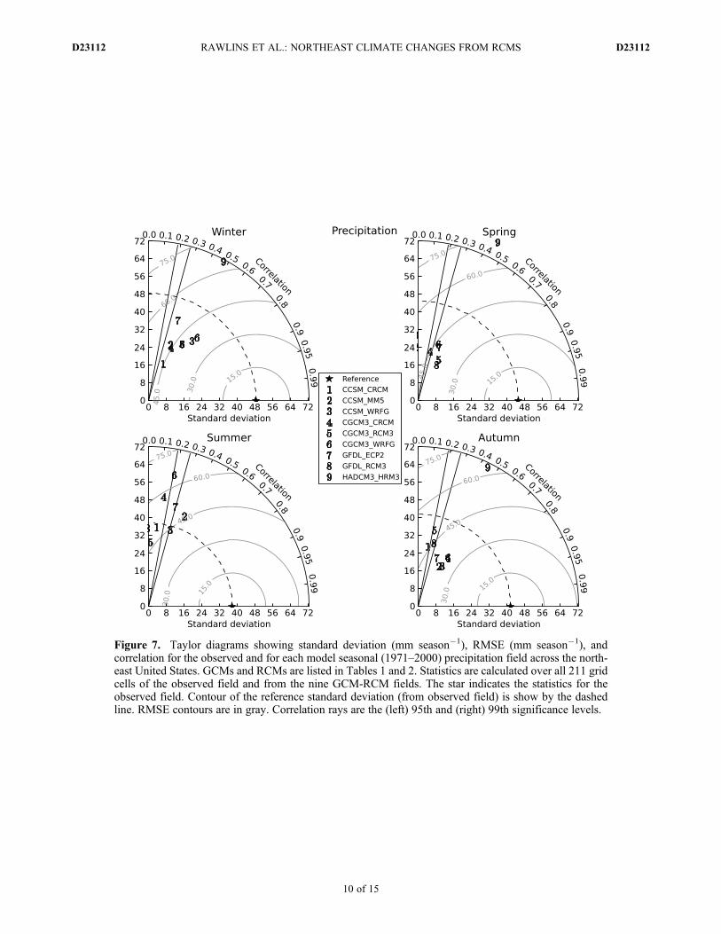
Figure 7. Taylor diagrams showing standard deviation (mm season�1), RMSE (mm season�1), andcorrelation for the observed and for each model seasonal (1971–2000) precipitation field across the north-east United States. GCMs and RCMs are listed in Tables 1 and 2. Statistics are calculated over all 211 gridcells of the observed field and from the nine GCM-RCM fields. The star indicates the statistics for theobserved field. Contour of the reference standard deviation (from observed field) is show by the dashedline. RMSE contours are in gray. Correlation rays are the (left) 95th and (right) 99th significance levels.


10 of 15

Figure 8. Bias (mm season�1) in multimodel mean estimate of seasonal precipitation (1971–2000) atnortheast United States grid cells. Bias is defined (Pmodels - PUDel) / PUDel * 100%, where Pmodels is themultimodel mean precipitation for the grid. Stipling indicates a significant bias at 95% confidence levelbased on student t test. Data for observations are taken from the UDel 0.5 degree data set.


11 of 15

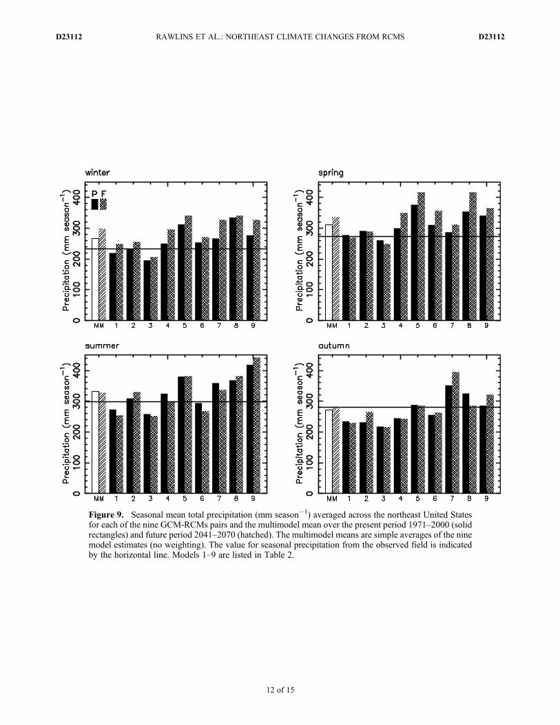
Figure 9. Seasonal mean total precipitation (mm season�1) averaged across the northeast United Statesfor each of the nine GCM-RCMs pairs and the multimodel mean over the present period 1971–2000 (solidrectangles) and future period 2041–2070 (hatched). The multimodel means are simple averages of the ninemodel estimates (no weighting). The value for seasonal precipitation from the observed field is indicatedby the horizontal line. Models 1–9 are listed in Table 2.


12 of 15

agreement mapping method [Tebaldi et al., 2011] winterprecipitation changes are significant and highest acrossinterior areas. For spring and autumn models agree on smallpositive changes, which are significant over much of theregion in spring and within the level of natural variability inautumn. The spatial change pattern in summer, with moderateprecipitation declines across Pennsylvania and lower chan-ges, relative to internal variability, to the north, presents aninteresting case for attribution study.[28] The magnitude and sign of seasonal precipitation

changes are broadly consistent with a recent study using nineIPCC AOGCMs which also showed projected increases in

winter precipitation and no change to a decrease in summerrainfall [Hayhoe et al., 2007]. Future increases in wintertemperature and precipitation would extend recent observeddecreases in the snowfall-to-precipitation ratio [Huntingtonet al., 2004]. Our results raise confidence in expectationsfor mid-century winter precipitation increases across thenortheast. Given the robust projections of winter air tem-perature increases, a continuation of the recent trend towardwetter and warmer winters [Hayhoe et al., 2007; Keim et al.,2005] appears likely. For summer the combination of 2–3�Cwarming and precipitation decreases approaching 10%across much of Pennsylvania would likely create severe

Figure 10. Distributions of precipitation (mm season�1) for the observed (O) and RCM present period(P) fields for period 1971–2000, and for the future period (F). Each distribution consists of 211 0.5 degreegrid cells spanning the northeast United States. Heavy line in each box is the distribution mean. Thin line(nearly identical to mean in most cases) is the distribution median. Boxes bracket the 25th and 75th per-centiles. Whiskers show the 5th and 95th percentiles.

Figure 11. REA change (%, D = P2041–2070 � P1971–2000/P1971–2000 ∗ 100%) in seasonal precipitationacross the northeast United States (solid circles); corresponding upper and lower REA uncertainty limits(horizontal lines); ensemble average changes (open circles); and estimated natural variability values(square). Units are percent of observed precipitation.


13 of 15

water stress to ecosystems. This study illustrates the impor-tance of using multiple model simulation estimates to gainunderstanding of likely changes in climate at decadal time-scales and smaller spatial scales.

[29] Acknowledgments. This research was supported by the Consor-tium for Climate Risk in the Urban Northeast (award NA10OAR4310212from the NOAA RISA program). The authors wish to thank the North Amer-ican Regional Climate Change Assessment Program (NARCCAP) for pro-viding the data used in this paper. NARCCAP is funded by the NationalScience Foundation (NSF), the U.S. Department of Energy (DoE), theNational Oceanic and Atmospheric Administration (NOAA), and the U.S.Environmental Protection Agency Office of Research and Development(EPA). They also thank Fangxing Fan for comments on an earlier versionof the manuscript.

ReferencesAlley, R. B., et al. (2007), Summary for policy-makers, in Climate Change2007: The Physical Science Basis. Contribution of Working Group I tothe Fourth Assessment Report of the Intergovernmental Panel on ClimateChange, edited by S. Solomon et al., pp. 1–18, Cambridge Univ. Press,Cambridge, U. K.

Caya, D., and S. Biner (2004), Internal variability of RCM simulations overan annual cycle, Clim. Dyn., 22, 33–46, doi:10.1007/s00382-003-0360-2.

Christensen, J. H., E. Kjellström, F. Giorgi, G. Lenderink, and M.Rummukainen (2010), Weight assignment in regional climate models,Clim. Res., 44, 179–194.

Christensen, O. B., J. H. Christensen, B. Machenhauer, and M. Botzet (1998),Very high-resolution regional climate simulations over Scandinavia—Present climate, J. Clim., 11(12), 3204–3229, doi:http://dx.doi.org/10.1175/1520-0442(1998)011<3204:VHRRCS>2.0.CO;2.

Deser, C., A. Phillips, V. Bourdette, and H. Teng (2012), Uncertainty inclimate change projections: the role of internal variability, Clim. Dyn.,38, 527–546, doi:10.1007/s00382-010-0977-x.

Dickinson, R. E., G. A. Meehl, and W. M. Washington (1987), Ice-albedofeedback in a CO2 doubling simulation, Clim. Change, 10, 241–248,doi:10.1007/BF00143904.

Diffenbaugh, N. S., J. S. Pal, R. J. Trapp, and F. Giorgi (2005), Fine-scaleprocesses regulate the response of extreme events to global climate

change, Proc. Natl. Acad. Sci. U. S. A., 102(44), 15,774–15,778,doi:10.1073/pnas.0506042102.

Dominguez, F., E. Rivera, D. P. Lettenmaier, and C. L. Castro (2012),Changes in winter precipitation extremes for the western United Statesunder a warmer climate as simulated by regional climate models,Geophys. Res. Lett., 39, L05803, doi:10.1029/2011GL050762.

Frei, C., J. Hesselbjerg Christensen, M. Déqué, D. Jacob, R. G. Jones, andP. L. Vidale (2003), Daily precipitation statistics in regional climate models:Evaluation and intercomparison for the European Alps, J. Geophys. Res.,108(D3), 4124, doi:10.1029/2002JD002287.

Giorgi, F., and L. O. Mearns (2002), Calculation of average, uncertaintyrange, and reliability of regional climate changes from AOGCM simula-tions via the “reliability ensemble averaging” (REA) method, J. Clim.,15(10), 1141–1158.

Giorgi, F., and L. O. Mearns (2003), Probability of regional climate changebased on the reliability ensemble averaging (REA) method, Geophys.Res. Lett., 30(12), 1629, doi:10.1029/2003GL017130.

Giorgi, F., L. O. Mearns, C. Shields, and L. McDaniel (1998), Regionalnested model simulations of present day and 2 x CO2 climate over theCentral Plains of the US, Clim. Change, 40, 457–493.

Giorgi, F., et al. (2001), Regional Climate Information—Evaluation andProjections, edited by J. T. Houghton et al., 881 pp., Cambridge Univ.Press, Cambridge, U. K.

Giorgi, F., J. Coln, and A. Ghassem (2009), Addressing climate informationneeds at the regional level. the cordex framework, WMO Bull., 58(3),175–183.

Gutowski, W. J., et al. (2010), Regional extreme monthly precipitationsimulated by NARCCAP RCMs, J. Hydrometeorol., 11, 1373–1379,doi:10.1175/2010JHM1297.1.

Hall, A. (2004), The role of surface albedo feedback in climate, J. Clim.,17, 1550–1568, doi:http://dx.doi.org/10.1175/1520-0442(2004)017<1550:TROSAF>2.0.CO;2.

Hawkins, E., and R. Sutton (2009), The potential to narrow uncertainty inregional climate predictions, Bull. Am. Meteorol. Soc., 90, 1095–1107,doi:10.1175/2009BAMS2607.1.

Hawkins, E., and R. Sutton (2011), The potential to narrow uncertainty inprojections of regional precipitation change, Clim. Dyn., 37, 407–418,doi:10.1007/s00382-010-0810-6.

Hayhoe, K., et al. (2007), Past and future changes in climate and hydro-logical indicators in the US Northeast, Clim. Dyn., 28, 381–407,doi:10.1007/s00382-006-0187-8.

Figure 12. Relative percent change (%, D = P2041–2070 � P1971–2000/P1971–2000 ∗ 100%) in seasonalprecipitation from the ensemble mean of the nine model pairs. Units are percent of present-day precipita-tion. Significance determined following criteria described by Tebaldi et al. [2011]. See text for details onmeaning behind the uncertainty and significance logic.


14 of 15

Huntington, T. G., G. A. Hodgkins, B. D. Keim, and R. W. Dudley (2004),Changes in the proportion of precipitation occurring as snow in NewEngland (1949 to 2000), J. Clim., 17, 2626–2636.

Keim, B. D., M. R. Fischer, and A. M. Wilson (2005), Are there spuriousprecipitation trends in the United States Climate Division database?,Geophys. Res. Lett., 32, L04702, doi:10.1029/2004GL021985.

Knutti, R., R. Furrer, C. Tebaldi, J. Cermak, and G. A. Meehl (2010),Challenges in combining projections from multiple climate models,J. Clim., 23(18), 2739–2758, doi:10.1175/2009JCLI3361.1.

Lenderink, G. (2012), Climate change: Tropical extremes, Nat. Geosci., 5,689–690, doi:10.1038/ngeo1587.

Li, G., X. Zhang, F. Zwiers, and Q. H. Wen (2012), Quantification ofuncertainty in high-resolution temperature scenarios for North America,J. Clim., 25(9), 3373–3389, doi:10.1175/JCLI-D-11-00217.1.

Liepert, B. G., and M. Previdi (2012), Inter-model variability and biases ofthe global water cycle in CMIP3 coupled climate models, Environ. Res.Lett., 7(1), 014006, doi:10.1088/1748-9326/7/1/014006.

Mearns, L. O. (2003), Issues in the impacts of climate variability andchange on agriculture, Clim. Change, 60, 1–7.

Mearns, L. O., F. Giorgi, L. McDaniel, and C. Shields (1995), Results fromthe model evaluation consortium for climate assessment, Global Planet.Change, 10(1–4), 55–78, doi:10.1016/0921-8181(94)00020-E.

Mearns, L. O., et al. (2007), The North American Regional Climate ChangeAssessment Program dataset, accessed 2 December 2011, http://www.earthsystemgrid.org/project/NARCCAP.html, NCAR, Boulder, Colo.

Mearns, L. O., W. J. Gutowski, R. Jones, L. R. Leung, S. McGinnis,A. Nunes, and Y. Qian (2009), A regional climate change assessmentprogram for North America, Eos Trans. AGU, 90(36), 311–312.

Mearns, L. O., et al. (2012), The North American Regional Climate ChangeAssessment Program: The overview of phase I results, Bull. Am.Meteorol. Soc., 93, 1337–1362, doi:10.1175/BAMS-D-11-00223.1.

Nakicenovic, N., et al. (2000), Special Report on Emissions Scenarios:A Special Report of Working Group III of the Intergovernmental Panelon Climate Change, Cambridge Univ. Press, Cambridge, U. K.

Plummer, D. A., D. Caya, A. Frigon, H. Côté, M. Giguère, D. Paquin,S. Biner, R. Harvey, and R. de Elia (2006), Climate and climate changeover North America as simulated by the Canadian RCM, J. Clim., 19,3112–3132, doi:10.1175/JCLI3769.1.

Rowlands, D. J., et al. (2012), Broad range of 2050 warming from anobservationally constrained large climate model ensemble, Nat. Geosci.,5, 256–260, doi:10.1038/ngeo1430.

Roy, P., P. Gachon, and R. Laprise (2011), Assessment of summer extremesand climate variability over the north-east of North America as simulatedby the Canadian Regional Climate Model, Int. J. Climatol., 32(11),1615–1627, doi:10.1002/joc.2382.

Sobolowski, S., and T. M. Pavelsky (2012), Evaluation of present andfuture North American Regional Climate Change Assessment Program(NARCCAP) regional climate simulations over the southeast UnitedStates, J. Geophys. Res., 117, D01101, doi:10.1029/2011JD016430.

Tebaldi, C., and R. Knutti (2007), The use of the multi-model ensemblein probabilistic climate projections, Philos. Trans. R. Soc. A, 365,2053–2075, doi:10.1098/rsta.2007.2076.

Tebaldi, C., J. M. Arblaster, and R. Knutti (2011), Mapping model agree-ment on future climate projections, Geophys. Res. Lett., 38, L23701,doi:10.1029/2011GL049863.

Willmott, C. J., and K. Matsuura (1995), Smart interpolation of annuallyaveraged air temperature in the United States, J. Appl. Meterol., 34,811–816.

Willmott, C. J., and S. M. Robeson (1995), Climatologically aided interpo-lation (CAI) of terrestrial air temperature, Int. J. Climatol., 15, 221–229.

Wood, A. W., L. R. Leung, V. Sridhar, and D. P. Lettenmaier (2004),Hydrologic implications of dynamical and statistical approaches to down-scaling climate model outputs, Clim. Change, 62, 189–216, doi:10.1023/B:CLIM.0000013685.99609.9e.


15 of 15

Documents

Assessment of regional climate model simulation … of regional climate model simulation estimates ... climate model simulation estimates over ... or statistical methods. Statistical