CHAPTER 4 SPECTRAL HISTOGRAM: A GENERIC FEATURE FOR …fsvision.fsu.edu/publications/papers/dissertation/chapter04.pdf · histogram for each local window in the pyramid. We obtain

CHAPTER 4

SPECTRAL HISTOGRAM: A GENERIC FEATURE FOR

IMAGES

In this chapter, we propose a generic statistic feature for homogeneous texture im-

ages, which we call spectral histograms. A similarity measure between any given image

patches is then defined as the Kullback-Leibler divergence or other distance measures

between the corresponding spectral histograms. Unlike other similarity measures,

it can discriminate texture as well as intensity images and provide a unified, non-

parametric similarity measure for images. We demonstrate this using examples in

texture image synthesis [147], texture image classification, and content-based image

retrieval. We compare several different distance measures and find that the spectral

histogram is not sensitive to the particular form of distance measure. We also com-

pare the spectral histogram with other statistic features and find that the spectral

histogram gives the best result for classification of a texture image database. We find

that distribution of local features is important while the local features themselves do

not appear to be critically important for texture discrimination and classification.

75

4.1 Introduction

As discussed in Chapter 1, the ultimate goal of a machine vision system is to

derive a description of input images. To build an efficient and effective machine vision

system, a critical step is to derive meaningful features. Here “meaningful” states that

the high-level modules such as recognition should be able to use the derived features

readily. To illustrate the problem, Figure 1.1(a) shows a texture image and a small

patch from 1.1(a) is shown in Figure 1.1(b). Figure 1.1(c) shows the numerical values

of (b). It is extremely difficult, if not impossible, to derive a segmentation or useful

representation for the given image purely based on the numerical values. This example

demonstrates that features need to be extracted based on input images for machine

vision systems as well as for biological vision systems.

While many algorithms and systems have been proposed for image segmentation,

classification, and recognition, feature extraction is not well addressed. In most cases,

features are chosen by assumption for mathematical convenience or domain-specific

heuristics. For example, Canny [13] derived the most widely used edge detection

algorithm based on a step edge with additive Gaussian noise. Using variational tech-

niques, he obtained the optimal filter for the assumed model and proposed the first-

order derivative of Gaussian as an efficient and good approximation. Inspired by

the neurophysiological experimental findings of on- and off-center simple cells [54]

[53], Marr and Hildreth [89] proposed the second-order derivative of Gaussian (LoG,

Laplacian of Gaussian) to model the responses of the on- and off-center cells. This

simple, piece-wise constant model has been widely used in image segmentation al-

gorithms. For example, Mumford and Shah [94] proposed an energy functional for

76

image segmentation

E(f, Γ) = µ∫ ∫

R(f − I)2dxdy +

∫ ∫

R\Γ‖ ∇f ‖2 dxdy + ν|Γ|. (4.1)

Here I is a two-dimensional input image defined on R, and f is the solution to be

found and Γ is the boundary of f . One can see that the underlying assumption of

the solution space is piece-wise smooth images. The energy functional shown in (4.1)

was claimed to be a generic energy functional [92] in that most existing segmentation

algorithms and techniques can be derived from the proposed energy functional.

Another major line of research related to feature extraction is texture discrimina-

tion and classification/segmentation. There are no obvious features that work well

for all texture images. The human visual system, however, can discriminate textures

robustly and effectively. This observation inspired many research activities. Julesz

[62] pioneered the research in searching for feature statistics for human visual per-

ception. He first studied k-gon statistics and conjectured that k = 2 is sufficient for

human visual perception. The conjecture was experimentally disproved by synthesiz-

ing perceptually different textures with identical 2-gon statistics [11] [24]. Other early

features for texture discrimination include co-occurrence matrices [44] [43], first-order

statistics [61], second-order statistics [18], and Markov random fields [65] [21] [16].

Those features have limited expressive power due to that the analysis of spatial inter-

action is limited to a relatively small neighborhood [147] and are applied successfully

to so-called micro-textures.

In the 1980s, theories on human texture perception were established, largely

based on available psychophysical and neurophysiological data [12] [23] and joint

spatial/frequency representation. Theories state that the human visual system trans-

forms the retinal image into local spatial/frequency representation, which can be

77

computationally simulated by convolving the input image with a bank of filters with

tuned frequencies and orientations. The mathematical framework for the local spa-

tial/frequency was laid out by Gabor [33] in the context of communication systems.

In Fourier transform, a signal can be represented in time and frequency domains. The

basis functions in time domain are impulses with different time delays, and the basis

functions in frequency domain are complex sinusoid functions with different frequen-

cies. A major problem with Fourier transform is localization. As shown in Figure

4.1, while the impulse in time domain precisely localizes the signal component, its

Fourier transform does not provide any localization information in frequency domain.

While the sinusoid function provides accurate localization in frequency domain, it

is not possible to localize the signal in time domain. Essentially, Fourier transform

uses two basis functions, which provides best localization in one domain and no lo-

calization in the other. Based on this observation, Gabor proposed a more generic

time/frequency representation [33], where the basis functions of Fourier transforms

are just two opposite extremes. By minimizing the localization uncertainty both in

time and frequency domains, Gabor proposed basis functions, which can achieve the

optimality simultaneously in time and frequency domains. Gabor basis functions were

extended to two-dimensional images by Daugman [22]. Very recently, this theory has

also been confirmed by deriving similar feature detectors from natural images based

on certain optimization criteria [100] [101] [102] [1].

The human perception theory and the local spatial/frequency representational

framework inspired much research in texture classification and segmentation. Within

this framework, however, statistic features still need to be chosen due to that filter

78

(a)

(b)

Figure 4.1: Basis functions of Fourier transform in time and frequency domains withtheir Fourier transforms. (a) An impulse and its Fourier transform. (b) A sinusoidfunction and its Fourier transform.

79

responses are not homogeneous within homogeneous textures and not sufficient be-

cause they are linear. As shown in Figure 4.2, a Gabor filter, shown in Figure 4.2(b),

responses to local and oriented structures, as shown in Figure 4.2(c), and the filter

response itself does not characterize the texture. Intuitively, texture appearance can

not be characterized by very local pixel values because texture is a regional prop-

erty. If we want to define a feature that is homogeneous within a texture region, it

is necessary to integrate responses from filters with multiple orientations and scales.

In other words, features need to be defined as statistic measures on filter responses.

For example, Unser [127] used variances from different filters to characterize textures.

Ojala et al [99] compared different features for texture classification using the distri-

bution of detected local features using a database consisting of nine images. Puzicha

et al [107] used a distribution of responses from a set of Gabor filters as features.

However, they posed the texture segmentation as an energy minimization based on a

pair-wise discrimination matrix, and the features used are not analyzed in terms of

characterizing texture appearance.

Recently, Heeger and Bergen [45] proposed a texture synthesis algorithm that can

match texture appearance. The algorithm tries to transform a random noisy image

into an image with similar appearance to the given target image by matching inde-

pendently the histograms of image pyramids constructed from the noisy and target

images. The experimental results are impressive even though no theoretical justifi-

cation was given. De Bonet and Viola [8] attempted to match the joint histograms

by utilizing the conditional probability defined on parent vectors. A parent vector is

a vector consisting of the filter responses in the constructed image pyramid up to a

80

��

0

5

10

15

20

0

5

10

15

20−1

−0.5

0

0.5

1

1.5

��

(a) (b) (c)

Figure 4.2: A texture image with its Gabor filter response. (a) Input texture image.(b) A Gabor filter, which is truncated to save computation. (c) The filter responseobtained through convolution.

given scale. As pointed out by Zhu et al. [147], these methods do not guarantee to

match the proposed statistics closely.

Zhu et al. [148] [149] [150] proposed a theory for learning probability models by

matching histograms based on maximum entropy principle and a FRAME (Filters,

Random field, And Maximum Entropy) model is developed for texture synthesis. To

avoid the computational problem of learning the Lagrange multipliers in the FRAME

model, Julesz ensemble is defined as the set of texture images that have the same

statistics as the observed images [147]. It demonstrates through experiments that

feature pursuit and texture synthesis can be done effectively by sampling from the

Julesz ensemble using MCMC (Monte-Carlo Markov Chain) sampling. It has been

shown that the Julesz ensemble is consistent with the FRAME model [143].

In this chapter, inspired by the FRAME model [148] [149] [150] and especially the

texture synthesis model [147], we define a feature, what we call spectral histograms.

Given a window in an input image centered around a given pixel, we construct a

81

pyramid based on the local window using a bank of chosen filters. We calculate the

histogram for each local window in the pyramid. We obtain a vector, consisting of

the histograms from all filters, which is defined as spectral histogram at the given

location.

For chosen statistic features to be used for successive modules, such as classifica-

tion, segmentation, and recognition, a similarity/distance measure must be defined.

A distance measure between two spectral histograms is defined as the χ2-statistic or

other distance measures between the spectral histograms. A distance measure using

χ2-statistic was proposed based on empirical experiments [107] [50]. However, as we

will demonstrate using classification, the particular form of distance measure is not

critical for spectral histograms.

In Section 4.2, we formally define spectral histograms and give some properties

of spectral histograms. In Section 4.3 we show how to synthesize texture images

by matching spectral histograms. In Section 4.4, we study spectral histograms for

texture classification. In Section 4.5, we apply spectral histograms to the problem of

content-based image retrieval. In Section 4.6, we compare different texture features

and different similarity measures using classification. In Section 4.7, we apply our

model to synthetic texture pair discrimination. Section 4.8 concludes this chapter

with further discussion.

4.2 Spectral Histograms

Given an input image I, defined on a finite two-dimensional lattice, and a bank

of filters {F (α), α = 1, 2, . . . , K}, a sub-band image I(α) is computed for each filter

through linear convolution, i.e., I(α)(v) = F (α) ∗ I(v) =∑

u F (u)I(v − u). I(α), α =

82

1, 2, . . . , K can be considered as an image pyramid constructed from the given image

I when there exist scaling relationships among the chosen filters. Here we loosely call

I(α), α = 1, 2, . . . , K as an image pyramid for an arbitrary chosen bank of filters. For

each sub-band image, we define the marginal distribution, or histogram

H(α)I

(z) =1

|I|∑

v

δ(z − I(α)(v)). (4.2)

We then define the spectral histogram with respect to the chosen filters as

HI = (H(1)I

, H(2)I

, . . . , H(K)I

). (4.3)

Spectral histograms of an image or an image patch are essentially a vector con-

sisting of marginal distributions of filter responses. The size of the input image or

the input image patch is called integration scale. We define a similarity measure be-

tween two spectral histograms using different standard distance measures. Lp-norm

distance is defined as

|HI1−HI2

|p =K∑

α=1

(

∑

z

(H(α)I1

(z)−H(α)I2

(z))p

)(1/p)

. (4.4)

Also because marginal distribution of each filter response is a distribution, a dis-

tance can be defined based on discrete Kullback-Leibler divergence [70]

KL(HI1, HI2

) =K∑

α=1

∑

z

(H(α)I1

(z)−H(α)I2

(z)) logH

(α)I1

(z)

H(α)I2

(z). (4.5)

Another choice for distance is χ2-statistic, which is a first-order approximation of

Kullback-Leibler divergence and is used widely to compare histograms

χ2(HI1, HI2

) =K∑

α=1

∑

z

(H(α)I1

(z)−H(α)I2

(z))2

H(α)I1

(z) + H(α)I2

(z). (4.6)

83

��

0

5

10

15

20

0

5

10

15

20−1

−0.5

0

0.5

1

1.5

(a) (b) (c)

(d)

Figure 4.3: A texture image and its spectral histograms. (a) Input image. (b) AGabor filter. (c) The histogram of the filter. (d) Spectral histograms of the image.There are eight filters including intensity filter, gradient filters Dxx and Dyy, fourLoG filters with T =

√2/2, 1, 2, and 4, and a Gabor filter Gcos(12, 150◦). There

are 8 bins in the histograms of intensity and gradient filters and 11 bins for the otherfilters.

84

4.2.1 Properties of Spectral Histograms

Images sharing the same spectral histograms define an ensemble, called Julesz

ensemble [147]. Equivalence between Julesz ensemble and the FRAME model [149]

[150] has been established [143].

As proven in [150], the true probability model of one type of texture images can

be approximated by linear combinations of marginal distributions given in spectral

histograms. In other words, spectral histograms provide a set of “basis functions” for

statistic modeling of texture images.

The spectral histogram and the associated distance measure provide a unified

similarity measure for images. Because the marginal distribution is independent of

image sizes, any two image patches can be compared using the spectral histogram.

Naturally, we can define a scale space using different integration scales, which can be

used to measure the homogeneity. This will be studied in the next chapter.

Due to that spectral histograms are based on marginal distributions, they pro-

vide a statistical measure and two images do not need to be aligned in order to be

compared.

4.2.2 Choice of Filters

The filters used consist of filters that are consistent with the human perception

theory. Following Zhu et al [149], we use four kinds of filters.

1. The intensity filter, which is the δ() function and captures the intensity value

at a given pixel.

2. Difference or gradient filters. We use four of them:

85

Dx = C · [0.0 − 1.0 1.0]

Dy = C ·

0.0−1.0

1.0

Dxx = C · [−1.0 2.0 − 1.0].

Dyy = C ·

−1.02.0−1.0

Here C is a normalization constant.

3. Laplacian of Gaussian filters:

LoG(x, y|T ) = C · (x2 + y2 − T 2)e−x2+y2

T2 , (4.7)

where C is a constant for normalization and T =√

2σ determines the scale

of the filter and σ is the variance of the Gaussian function. These filters are

referred to as LoG(T ).

4. The Gabor filters with both sine and cosine components:

Gabor(x, y|T, θ) = C · e− 1

2T2 (4(x cos θ+y sin θ)2+(−x cos θ+y sin θ)2)e−i 2πT

(x cos θ+y sin θ).

(4.8)

Here C is a normalization constant and T is a scale. These filters are referred

to as Gcos(T, θ) and Gsin(T, θ).

While there may exist an optimal set for a given texture, we do not change filters

within a task. In general, we use more filters for texture synthesis, namely 56 filters.

We use around 8 filters for texture classification and content-based image retrieval

to save computation. More importantly, it seems unnecessary to use more filters

86

for texture classification and content-based image retrieval when relatively a small

integration scale is used.

4.3 Texture Synthesis

In this section we demonstrate the effectiveness of the spectral histogram in charac-

terizing texture appearance using texture synthesis. We define a relationship between

two texture images using the divergence between their spectral histograms. There ex-

ists such a relationship if and only if their spectral histograms are sufficiently close.

It is easy to check that this defines an equivalence class.

Given observed feature statistics, {H (α)obs , α = 1, ..., K}, which are spectral his-

tograms computed from observed images, we define an energy function [147]

E(I) =K∑

α=1

D(H(α)(I) , H

(α)obs). (4.9)

Then the corresponding Gibbs distribution is

q(I) =1

ZΘ

exp(−E(I)Θ

) (4.10)

where Θ is the temperature.

The Gibbs distribution can be sampled by a Gibbs sampler or other MCMC

algorithms. Here we use a Gibbs sampler [147] given in Figure 4.4. In Figure 4.4,

q(Isyn(v) | Isyn(−v)) is the conditional probability of pixel values at v given the rest

of the image. D is a distance measure and L1-norm is used for texture synthesis.

For texture synthesis, we use 56 filters:

• The intensity filter.

• 4 gradient filters.

87

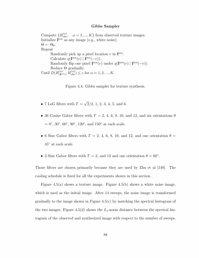
Gibbs Sampler

Compute {H(α)obs , α = 1, ..., K} from observed texture images.

Initialize Isyn as any image (e.g., white noise).Θ← Θ0.Repeat

Randomly pick up a pixel location v in Isyn.Calculate q(Isyn(v) | Isyn(−v)).Randomly flip one pixel Isyn(v) under q(Isyn(v) | Isyn(−v)).Reduce Θ gradually.

Until D(H(α)(Isyn), H

(α)obs) ≤ ε for α = 1, 2, ..., K.

Figure 4.4: Gibbs sampler for texture synthesis.

• 7 LoG filters with T =√

2/2, 1, 2, 3, 4, 5, and 6.

• 36 Cosine Gabor filters with T = 2, 4, 6, 8, 10, and 12, and six orientations θ

= 0◦, 30◦, 60◦, 90◦, 120◦, and 150◦ at each scale.

• 6 Sine Gabor filters with T = 2, 4, 6, 8, 10, and 12, and one orientation θ =

45◦ at each scale.

• 2 Sine Gabor filters with T = 2, and 12 and one orientation θ = 60◦.

Those filters are chosen primarily because they are used by Zhu et al [149]. The

cooling schedule is fixed for all the experiments shown in this section.

Figure 4.5(a) shows a texture image. Figure 4.5(b) shows a white noise image,

which is used as the initial image. After 14 sweeps, the noise image is transformed

gradually to the image shown in Figure 4.5(c) by matching the spectral histogram of

the two images. Figure 4.5(d) shows the L1-norm distance between the spectral his-

togram of the observed and synthesized image with respect to the number of sweeps.

88

The matched error decreases at an exponential rate, demonstrating the synthesis al-

gorithm is computationally efficient. One can see that the synthesized image shown in

Figure 4.5(c) is perceptually similar to the observed image. By matching the spectral

histogram, synthesized image captures the textural elements and their arrangement

and gives similar perceptual appearance.

Figure 4.6 shows the temporal evolution of a Gabor filter. Figure 4.6(a) shows

the filter, which is truncated to save computation. Figure 4.6(b) shows the histogram

of the filter at different sweeps. Figure 4.6(c) shows the matching error of the filter.

Figure 4.6(d) shows the differences of histograms of the observed and synthesis images,

which is multiplied by 1000 for display purposes. The biggest error among the bins

is less than 0.0003.

Figure 4.7 shows three more texture images and the synthesized images from the

algorithm. The synthesized images are perceptually similar to the observed images

and their spectral histograms match closely. In Figure 4.7(b), due to local minima,

there are local regions which are not reproduced well.

Figure 4.8 shows two texture examples with regular patterns. The texture image

in Figure 4.8(a) shows a very regular leather surface. The synthesized image after

20 sweeps shown in Figure 4.8(a) is perceptually similar to the input texture. But

the regularity of patterns is blurred and each element is not as clear as in the input

image. However, the two images give quite similar percepts and the synthesized im-

age captures the essential arrangement of patterns and the prominent edges in the

input. Figure 4.8(b) shows an example where the vertical long-range arrangements

are promising. While the synthesized image captures the local vertical arrangements,

89

(a) (b)

0 2 4 6 8 10 12 140

5

10

15

20

25

(c) (d)

Figure 4.5: Texture image synthesis by matching observed statistics. (a) Observedtexture image. (b) Initial image. (c) Synthesized image after 14 sweeps. (d) Thetotal matched error with respect to sweeps.

90

0

5

10

15

20

0

5

10

15

20−1

−0.5

0

0.5

1

1.5

1 2 3 4 5 6 7 8 9 10 110

0.05

0.1

0.15

0.2

0.25

(a) (b)

0 2 4 6 8 10 12 140

0.1

0.2

0.3

0.4

0.5

0.6

0.7

0.8

0.9

1

1 2 3 4 5 6 7 8 9 10 11−0.3

−0.25

−0.2

−0.15

−0.1

−0.05

0

0.05

0.1

0.15

0.2

(c) (d)

Figure 4.6: Temporal evolution of a selected filter for texture synthesis. (a) A Gaborfilter. (b) The histograms of the Gabor filter. Dotted line - observed histogram,which is covered by the histogram after 14 sweeps; dashed line - initial histogram;dash-dotted line - histogram after 2 sweeps. solid line - histogram after 14 sweeps.(c) The error of the chosen filter with respect to the sweeps. (d) The error betweenthe observed histogram and the synthesized one after 14 sweeps. Here the error ismultiplied by 1000.

91

(a)

(b)

(c)

Figure 4.7: More texture synthesis examples. Left column shows the observed imagesand right column shows the synthesized image within 15 sweeps. In (b), due to localminima, there are local regions which are not perceptually similar to the observedimage.

92

it does not sufficiently capture the long-range arrangements due to that the synthe-

sized algorithm is purely local and long-range couplings are almost impossible to be

captured.

While the texture images shown above are homogeneous textures, Figure 4.9(a)

shows an intensity image consisting of several regions. Figure 4.9(c) shows the syn-

thesized image after 100 sweeps. While the spectral histogram does not capture the

spatial relationships between different regions, big regions with similar gray values

emerge along the temporal evolution. Due to the inhomogeneity, the Gibbs sam-

pler converges slower compared with homogeneous texture images as shown in Figure

4.5(d).

Figure 4.10 shows a synthesized image for a synthetic texton image. In order to

synthesize a similar texton, Zhu et al [149] [150] used a texton filter which is the

template of one texton element. Here we use the same filters as for other images. As

shown in Figure 4.10(b), the texton elements are reproduced well except in two small

regions where the MCMC is trapped into a local minimum. This example clearly

demonstrates that spectral histograms provide a generic feature for different types of

textures, eliminating the need for ad hoc features for a particular set of textures.

Figure 4.11 shows a synthetic example where there are two distinctive regions in

the original. As shown in Figure 4.11(b), the synthesized image captures the appear-

ance of both regions using the spectral histogram. Here the boundary between two

regions is not reproduced because spectral histograms do not incorporate geometric

constraints. Using some geometric constraints, the boundary may be reproduced well,

which would give a more powerful feature for images consisting of different regions.

Figure 4.12 shows an interesting result for a face image. While all the “elements” are

93

��

��

(a) ��

(b)

Figure 4.8: Real texture images of regular patterns with synthesized images after 20sweeps. (a) An image of a leather surface. The total matched error after 20 sweeps is0.082. (b) An image of a pressed calf leather surface. The total matched error after20 sweeps is 0.064.

94

(a) (b)

0 10 20 30 40 50 60 70 80 90 1000

10

20

30

40

50

60

70

80

(c) (d)

Figure 4.9: Texture synthesis for an image with different regions. (a) The observedtexture image. This image is not a homogeneous texture image and consists mainlyof two homogeneous regions. (b) The initial image. (c) Synthesized image after 100sweeps. Even though the spectral histogram of each filter is matched well, comparedto other images, the error is still large. Especially for the intensity filter, the erroris still about 7.44 %. The synthesized image is perceptually similar to the observedimage except the geometrical relationships among the homogeneous regions. (d) Thematched error with respect to the sweeps. Due to that the observed image is nothomogeneous, the synthesis algorithm converges slower compared with Figure 4.5(d).

95

(a) (b)

Figure 4.10: A synthesis example for a synthetic texton image. (a) The originalsynthetic texton image with size 128 × 128. (b) The synthesized image with size256× 256.

captured in the synthesized image, the result is not meaningful unless some geometric

constraints are incorporated. This will be investigated further in the future.

To evaluate the synthesis algorithm more systematically, we have applied it to all

the 40 texture images shown in Figure 4.16. To save space, the reduced images are

shown in Figure 4.13. These examples clearly demonstrate that spectral histograms

capture texture appearance well.

4.3.1 Comparison with Heeger and Bergen’s Algorithm

As pointed out by Zhu et al [147], Heeger and Bergen’s algorithm does not ac-

tually match any statistic features defined on the input image. On the other hand,

the synthesis algorithm described above characterizes texture appearance explicitly

through the spectral histogram of the observed image(s), as demonstrated using real

texture images. One critical difference is that our proposed algorithm provides a

statistic modeling of the observed image(s) in that the algorithm only needs to know

96

(a) (b)

Figure 4.11: A synthesis example for an image consisting of two regions. (a) Theoriginal synthetic image with size 128 × 128, consisting of two intensity regions. (b)The synthesized image with size 256× 256.

(a) (b)

Figure 4.12: A synthesis example for a face image. (a) Lena image with size 347×334.(b) The synthesized image with size 256× 256.

97

Fabric-0 Fabric-4 Fabric-7 Fabric-9 Fabric-15 Fabric-17 Fabric-18

Food-0 Food-5 Leaves-3 Leaves-8 Leaves-12 Leaves-13 Metal-0

Metal-2 Misc-0 Misc-2 Stone-5 Water-1 Water-2 Water-6

Water-8 Beachsand-2 Calfleath-1 Calfleath-2 Grass-1 Grass-7 Grave-5

Hexholes-2 Pigskin-1 Pigskin-2 Plasticbubs-13 Raffia-1 Raffia-2 Roughwall-5

Sand-1 Woodgrain-1 Woodgrain-2 Woolencloth-1 Woolencloth-2

Figure 4.13: The synthesized images of the 40 texture images shown in Figure 4.16.Here same filters and cooling schedule are used for all the images.

98

Observed Black Gray White

Error L1-norm RMS L1-norm RMS L1-norm RMS L1-norm RMS

Observed 0.00 % 0.00 0.10 % 54.2 0.10 % 54.2 0.11 % 55.4

Black 0.10 % 54.2 0.00 % 0.00 0.11 % 54.6 0.11 % 60.8

Gray 0.10 % 54.1 0.11 % 54.6 0.00 % 0.00 0.12 % 50.3

While 0.11 % 55.4 0.11 % 60.8 0.12 % 50.3 0.00 % 0.00

Table 4.1: L1-norm distance of the spectral histograms and RMS distance betweenimages.

the spectral histogram of the input image(s) and it does not need the input images

while Heeger and Bergen’s algorithm needs the input image.

For comparison, we use the texture image shown in Figure 4.3(a). For the pro-

posed algorithm, we synthesize images starting with different initial images, as shown

in Figure 4.14. One can see that different initial images are transformed into percep-

tually similar images by matching the spectral histogram, where the matching error

is shown in Figure 4.14(d). Table 4.1 shows the L1-norm distance of the histograms of

the observed and synthesized images and the Root-Mean-Square (RMS) distance of

the corresponding images. From Table 4.1, one can see clearly that even though the

rooted mean square distance is large between the observed and synthesized images

from different initial conditions, the corresponding L1-norm distance between their

spectral histograms is quite small. Given that the synthesized images are perceptu-

ally similar to the observed image, we conclude that spectral histograms provide a

statistic feature to characterize texture appearance.

For the same input image, we have also applied the algorithm by Heeger and

Bergen [45]. The implementation used here is by El-Maraghi [28]. Figure 4.15 (a)-

(c) show the synthesized images with different number of iterations. Compared to

99

��

=⇒

��

(a) ��

=⇒

��

(b) ��

=⇒

��

(c)

0 2 4 6 8 10 12 14 16 18 200

10

20

30

40

50

60

70

80

90

(d)

Figure 4.14: Synthesized images from different initial images for the texture imageshown in Figure 4.3(a). (a)-(c) Left column is the initial image and right column isthe synthesized image after 20 sweeps. (d) The matched error with respect to thenumber of sweeps.

100

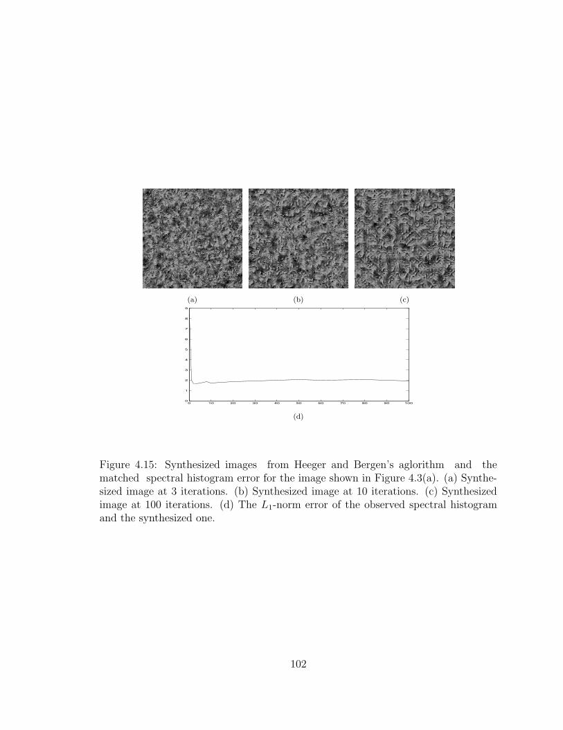
the synthesized images from our method shown in Figure 4.14(a)-(c), one can see

easily that the synthesized images in Figure 4.14(a)-(c) are perceptually similar to

the input texture image and capture texture elements and their distributions, while

the synthesized images in Figure 4.15 (a)-(c) are not percetually similar to the input

texture. As shown in Figure 4.15(d), the Heeger and Bergen’s algorithm does not

match the statistic features on which the algorithm is based and the error does not

decrease after 1 iteration. Because the Heeger and Bergen’s algorithm used Laplacian

of Gaussian paramid, we choose LoG and local filters for the spectral histogram here

for a fair comparison.

4.4 Texture Classification

Texture classification is closely related to texture segmentation and content-based

image retrieval. Here we demonstrate the discriminative power of spectral histograms.

A texture image database is given first and we extract spectral histograms for each

image in the database. The classification here is then to classify all the pixels or

selected pixels in an input image.

Given a database with M texture images, we represent each image by its average

spectral histogram Hobsm at a given integration scale. We use a minimum-distance

classifier, given by

m∗(v) = minm

D(HI(v), Hobsm). (4.11)

Here D is a similarity measure and χ2-statistic is used.

We use a texture image database available on-line at http://www-dbv.cs.uni-

bonn.de/image/texture.tar.gz. As shown in Figure 4.16, the database we use consists

of 40 texture images from Brodatz textures [10].

101

��

(a) (b) (c)

0 10 20 30 40 50 60 70 80 90 1000

1

2

3

4

5

6

7

8

9

(d)

Figure 4.15: Synthesized images from Heeger and Bergen’s aglorithm and thematched spectral histogram error for the image shown in Figure 4.3(a). (a) Synthe-sized image at 3 iterations. (b) Synthesized image at 10 iterations. (c) Synthesizedimage at 100 iterations. (d) The L1-norm error of the observed spectral histogramand the synthesized one.

102

Fabric-0 Fabric-4 Fabric-7 Fabric-9 Fabric-15 Fabric-17 Fabric-18

Food-0 Food-5 Leaves-3 Leaves-8 Leaves-12 Leaves-13 Metal-0

Metal-2 Misc-0 Misc-2 Stone-5 Water-1 Water-2 Water-6

Water-8 Beachsand-2 Calfleath-1 Calfleath-2 Grass-1 Grass-7 Grave-5 ��

Hexholes-2 Pigskin-1 Pigskin-2 Plasticbubs-13 Raffia-1 Raffia-2 Roughwall-5

Sand-1 Woodgrain-1 Woodgrain-2 Woolencloth-1 Woolencloth-2

Figure 4.16: Forty texture images used in the classification experiments. The inputimage size is 256× 256.

103

4.4.1 Classification at Fixed Scales

First we study the classification performance using the spectral histogram at a

given integration scale. As discussed above, the classification algorithm is a minimum

distance classifier and each location is classified independently from other locations.

For the database shown in Figure 4.16, we use a window of 35×35 pixels. For each

image in the database, we extract an average spectral histogram by averaging spectral

histograms extracted at a larger grid size to save computation. For classification and

content-based image retrieval, we use 8 filters to compute spectral histograms:

• The intensity filter.

• Two gradient filters Dxx and Dyy.

• Two LoG filters with T = 2 and 5.

• Three Cosine Gabor filters with T = 6 and three orientations θ = 30◦, 90◦, and

150◦.

Figure 4.17(a) shows the divergence between the feature vector of each image

numerically and Figure 4.17(b) shows the divergence in (a) as an image for easier

interpretation.

Each texture is divided into non-overlapping image patches with size 35 × 35.

Each image patch is classified into one of the 40 given classes using the minimum

distance classifier. Figure 4.18 shows the error rate for each image along with variance

within each image and minimum divergence of each image from the other images

in the database. The overall classification error is 4.2347%. As shown in Figure

104

4.18(a), the error is not evenly distributed. Five images, namely “Fabric-15”, “Leaves-

13”, “Water-1”, “Water-2”, and “Woolencloth-2” account for more than half of the

misclassified cases, with an average error of 19.18%. For the other 35 images, the

classification error is 2.10%.

There are two major reasons of the large error rates for the five images. First, with

respect to the given scale, which is 35× 35, the images are not homogeneous. Figure

4.18(b) shows the variance of the spectral histogram of images. Second, the image

is similar to some other images in the database. This is measured by the minimum

divergence between the feature vector of an image and the feature vector of the other

images. Figure 4.18(c) shows the minimum divergence. As shown clearly, the five

images with large classification error tend to have large variance and small minimum

divergence. The dotted curve in Figure 4.18(a) shows the ratio between the variance

and the minimum divergence of each image. The peaks in the classification error

curve tend to be coincident with the peaks in the ratio curve.

4.4.2 Classification at Different Scales

We also study the classification error with respect to different scales. We use 8

different integration scales in this experiment: 5× 5, 9× 9, 15× 15, 23× 23, 35× 35,

65 × 65, 119 × 119, and 217 × 217 in pixels. The classification algorithm and the

procedure are the same as described for the fixed scale.

The overall classification error is shown in Figure 4.19. As expected, the classifi-

cation error decreases when the scale increases. For spectral histograms, the classifi-

cation error decreases approximately at an exponential rate. This demonstrates that

spectral histograms are very good in capturing texture characteristics.

105

.0 4 2 11 2 5 3 5 3 10 3 7 7 4 6 7 2 1 4 7 4 5 9 3 9 5 1 5 11 3 10 3 3 9 4 4 5 7 2 9

4 .0 3 5 3 3 2 3 1 4 3 3 3 3 2 3 6 4 12 5 10 11 4 3 4 2 4 6 6 6 4 2 5 4 5 6 8 5 5 4

2 3 .0 8 2 3 1 3 1 7 4 5 4 2 3 4 4 2 9 5 8 8 6 1 6 3 2 5 8 3 7 2 2 6 4 4 6 5 2 6

11 5 8 .0 7 6 8 3 6 1 9 2 2 8 3 3 13 12 18 3 17 17 1 7 2 3 10 9 4 12 .8 6 10 1 8 11 13 3 11 .8

2 3 2 7 .0 4 3 3 2 7 2 4 4 4 3 4 3 2 9 5 7 8 6 2 6 3 1 4 9 3 7 .4 2 6 3 5 6 4 2 6

5 3 3 6 4 .0 2 4 2 6 5 4 4 2 3 5 7 5 12 4 11 10 5 2 4 2 5 7 7 5 5 4 4 5 5 6 6 4 5 4

3 2 1 8 3 2 .0 5 1 8 5 5 5 .5 4 6 5 2 9 6 8 8 7 2 6 3 3 7 8 4 7 4 3 7 6 5 6 6 3 6

5 3 3 3 3 4 5 .0 3 2 5 1 1 5 2 2 8 6 13 2 12 11 2 3 2 .7 5 5 6 6 2 2 4 2 4 7 8 3 5 2

3 1 1 6 2 2 1 3 .0 5 3 3 3 2 2 3 6 4 11 4 10 10 5 2 4 2 3 6 7 5 5 2 3 5 5 6 7 5 4 4

10 4 7 1 7 6 8 2 5 .0 7 .8 1 8 3 2 13 11 17 2 16 16 .6 6 2 3 9 8 4 11 .4 5 9 .8 7 10 12 4 10 .7

3 3 4 9 2 5 5 5 3 7 .0 5 5 5 5 4 4 4 10 6 7 9 8 4 8 5 2 5 9 4 8 2 4 8 4 5 7 6 4 8

7 3 5 2 4 4 5 1 3 .8 5 .0 .3 5 2 .8 10 8 15 2 14 14 1 4 1 .9 7 7 4 8 1 3 6 1 6 9 10 3 8 .8

7 3 4 2 4 4 5 1 3 1 5 .3 .0 5 1 1 9 8 15 .9 13 13 2 3 1 1 6 6 5 8 2 3 6 2 5 8 9 2 7 1

4 3 2 8 4 2 .5 5 2 8 5 5 5 .0 4 6 5 3 10 5 9 9 6 3 6 4 3 7 8 5 7 4 5 7 6 5 7 6 4 6

6 2 3 3 3 3 4 2 2 3 5 2 1 4 .0 2 8 7 14 2 12 13 2 3 2 1 5 7 5 8 3 3 6 2 6 8 9 3 7 2

7 3 4 3 4 5 6 2 3 2 4 .8 1 6 2 .0 9 8 14 3 13 13 3 4 3 2 6 6 5 8 3 3 6 3 6 8 9 4 7 2

2 6 4 13 3 7 5 8 6 13 4 10 9 5 8 9 .0 1 4 10 2 5 12 5 12 8 1 6 12 4 13 5 4 12 6 5 5 9 3 12

1 4 2 12 2 5 2 6 4 11 4 8 8 3 7 8 1 .0 5 8 4 5 10 3 10 6 1 7 11 3 11 4 4 10 6 4 5 8 2 10

4 12 9 18 9 12 9 13 11 17 10 15 15 10 14 14 4 5 .0 15 2 4 18 10 17 14 7 9 17 7 18 10 8 17 10 8 7 14 7 17

7 5 5 3 5 4 6 2 4 2 6 2 .9 5 2 3 10 8 15 .0 14 13 2 4 1 2 7 6 5 8 2 4 6 2 5 8 9 .8 7 1

4 10 8 17 7 11 8 12 10 16 7 14 13 9 12 13 2 4 2 14 .0 5 16 9 16 12 4 8 15 7 17 8 8 16 9 7 7 13 6 16

5 11 8 17 8 10 8 11 10 16 9 14 13 9 13 13 5 5 4 13 5 .0 16 9 16 12 7 7 15 4 16 9 6 16 7 6 4 13 4 16

9 4 6 1 6 5 7 2 5 .6 8 1 2 6 2 3 12 10 18 2 16 16 .0 6 .8 2 9 8 3 10 .3 5 8 .5 7 10 12 3 10 .3

3 3 1 7 2 2 2 3 2 6 4 4 3 3 3 4 5 3 10 4 9 9 6 .0 5 2 3 5 8 4 6 2 2 6 4 5 5 4 3 5

9 4 6 2 6 4 6 2 4 2 8 1 1 6 2 3 12 10 17 1 16 16 .8 5 .0 2 9 8 4 10 1 5 8 .9 7 9 11 2 9 .5

5 2 3 3 3 2 3 .7 2 3 5 .9 1 4 1 2 8 6 14 2 12 12 2 2 2 .0 5 5 5 6 2 2 4 2 4 7 8 3 5 2

1 4 2 10 1 5 3 5 3 9 2 7 6 3 5 6 1 1 7 7 4 7 9 3 9 5 .0 5 10 3 10 2 3 9 4 4 5 7 2 9

5 6 5 9 4 7 7 5 6 8 5 7 6 7 7 6 6 7 9 6 8 7 8 5 8 5 5 .0 10 3 8 4 4 8 .9 2 5 6 4 7

11 6 8 4 9 7 8 6 7 4 9 4 5 8 5 5 12 11 17 5 15 15 3 8 4 5 10 10 .0 11 4 8 10 3 10 10 12 7 11 4

3 6 3 12 3 5 4 6 5 11 4 8 8 5 8 8 4 3 7 8 7 4 10 4 10 6 3 3 11 .0 11 4 1 10 2 3 3 8 .7 10

10 4 7 .8 7 5 7 2 5 .4 8 1 2 7 3 3 13 11 18 2 17 16 .3 6 1 2 10 8 4 11 .0 6 9 .6 8 10 12 4 10 .3

3 2 2 6 .4 4 4 2 2 5 2 3 3 4 3 3 5 4 10 4 8 9 5 2 5 2 2 4 8 4 6 .0 3 5 3 5 7 4 3 5

3 5 2 10 2 4 3 4 3 9 4 6 6 5 6 6 4 4 8 6 8 6 8 2 8 4 3 4 10 1 9 3 .0 8 2 3 3 6 .9 8

9 4 6 1 6 5 7 2 5 .8 8 1 2 7 2 3 12 10 17 2 16 16 .5 6 .9 2 9 8 3 10 .6 5 8 .0 7 10 11 3 9 .5

4 5 4 8 3 5 6 4 5 7 4 6 5 6 6 6 6 6 10 5 9 7 7 4 7 4 4 .9 10 2 8 3 2 7 .0 3 3 5 3 7

4 6 4 11 5 6 5 7 6 10 5 9 8 5 8 8 5 4 8 8 7 6 10 5 9 7 4 2 10 3 10 5 3 10 3 .0 4 8 3 9

5 8 6 13 6 6 6 8 7 12 7 10 9 7 9 9 5 5 7 9 7 4 12 5 11 8 5 5 12 3 12 7 3 11 3 4 .0 8 3 11

7 5 5 3 4 4 6 3 5 4 6 3 2 6 3 4 9 8 14 .8 13 13 3 4 2 3 7 6 7 8 4 4 6 3 5 8 8 .0 7 3

2 5 2 11 2 5 3 5 4 10 4 8 7 4 7 7 3 2 7 7 6 4 10 3 9 5 2 4 11 .7 10 3 .9 9 3 3 3 7 .0 9

9 4 6 .8 6 4 6 2 4 .7 8 .8 1 6 2 2 12 10 17 1 16 16 .3 5 .5 2 9 7 4 10 .3 5 8 .5 7 9 11 3 9 .0

(a)

(b)

Figure 4.17: The divergence between the feature vector of each image in the textureimage database shown in Figure 4.16. (a) The cross-divergence matrix shown innumerical values. (b) The numerical values are displayed as an image.

106

0 5 10 15 20 25 30 35 400

2

4

6

8

10

12

(a)

0 5 10 15 20 25 30 35 400

0.5

1

1.5

2

2.5

3

3.5

4

4.5

(b)

0 5 10 15 20 25 30 35 400

0.5

1

1.5

2

2.5

3

3.5

4

(c)

Figure 4.18: (a) The classification error for each image in the texture database alongwith the ratio between the maximum and minimum divergence shown in (b) and (c)respectively. (b) The maximum divergence of spectral histogram from the featurevector of each image. (c) The minimum divergence between each image and the otherones.

107

0 50 100 150 200 2500

0.1

0.2

0.3

0.4

0.5

0.6

0.7

Figure 4.19: The classification error of the texture database with respect to the scalefor feature extraction.

As one would expect, the classification error with respect to scales varies consid-

erably for images. For example, image “Hexholes-2”, shown in Figure 4.20(a), is very

homogeneous and visually very different from other images in the database. For this

image, the classification result is good for all the scales used in the experiment. Even

using a window of 5 × 5 pixels, the classification error is 1.61%. At all other scales,

the classification is 100% correct, as shown in Figure 4.20(b).

Figure 4.21(a) shows image “Woolencloth-2” from the database. This image is

not homogeneous and perceptually similar to some other images. For this image, the

classification error is large when the scale is small. When the scale is 35 × 35, the

classification error is 20.41%. When the scale is larger than 35× 35, the classification

result is perfect, as shown in Figure 4.21(b).

4.4.3 Image Classification

In this section, we classify images using the database. Each pixel in the image

is classified using the minimum distance classifier. A window centered at a given

108

(a)

0 50 100 150 200 2500

0.002

0.004

0.006

0.008

0.01

0.012

0.014

0.016

0.018

0 50 100 150 200 2500

0.5

1

1.5

2

2.5

3

(b) (c)

Figure 4.20: (a) Image “Hexholes-2” from the texture database. (b) The classificationerror rate for the image. (c) The ratio between maximum divergence and minimumcross divergence with respect to scales.

109

(a)

0 50 100 150 200 2500

0.1

0.2

0.3

0.4

0.5

0.6

0.7

0.8

0.9

1

0 50 100 150 200 2500

20

40

60

80

100

120

140

160

180

(b) (c)

Figure 4.21: (a) Image “Woolencloth-2” from the texture database. (b) The clas-sification error rate for the image. (c) The ratio between maximum divergence andminimum cross divergence with respect to scales.

110

pixel is used. For pixels near image borders, a window that is inside the image and

contains the pixel is used. The input texture image, shown in Figure 4.22(a) con-

sists of five texture regions from the database. Figure 4.22(b) shows the classification

result, Figure 4.22(c) shows the divergence between the spectral histogram and the

feature vector of the assigned texture image. Figure 4.22(d) shows the ground truth

segmentation and Figure 4.22(e) shows the misclassified pixels, which are shown in

black. One can see that the interior pixels in each homogeneous texture region are

classified correctly and the divergence of these pixels is small. Only the pixels that

are between texture regions are misclassified due to that the spectral histogram com-

puted is a mixture of different texture regions. At misclassified pixels, the divergence

is large. This demonstrates that the proposed spectral histogram is a reliable sim-

ilarity/dissimilarity measure between texture images. Furthermore, it also provides

a reliable measure for goodness of the classification. The classification result can be

improved by incorporating context-sensitive feature detectors, as discussed in Section

5.6.

4.4.4 Training Samples and Generalization

For the classification results shown in this section, training samples are not sepa-

rated clearly from samples for testing due to the limited number of samples especially

at large integration scales. Through experiments, we demonstrate that the number

of training samples is not critical using spectral histograms.

First we re-do some of the experiments for classification. Here we use half of

the samples for training and do the testing on the remaining half. Figure 4.23(a)

shows the classification error for each image at integration scale 35 × 35 and Figure

111

(a) (b)

(c) (d)

(e)

Figure 4.22: (a) A texture image consisting of five texture regions from the texturedatabase. (b) Classification result using spectral histograms. (c) Divergence betweenspectral histograms and the feature vector of the assigned texture image. (d) Theground truth segmentation of the image. (e) Misclassified pixels, shown in black.

112

0 5 10 15 20 25 30 35 400

0.05

0.1

0.15

0.2

0.25

0 10 20 30 40 50 60 700

0.1

0.2

0.3

0.4

0.5

0.6

0.7

(a) (b)

Figure 4.23: (a) The classification error for each image in the database at integrationscale 35×35. (b) The classification error at different integration scales. In both cases,solid line – training is done using half of the samples; dashed line – training is doneusing all the samples.

4.23(b) shows the overall error at different integration scales along with the results

shown before. While the classification error varies from image to image using different

training samples, the overall classification error does not change much.

We also examine the influence of the ratio of testing samples to training samples.

Figure 4.24 shows the classification error with respect to the ratio of testing samples

to training samples at integration scales 23 × 23 and 35 × 35. It demonstrates that

the spectral histogram captures texture characteristics well from a small number of

training samples.

4.4.5 Comparison with Existing Approaches

Recently, Randen and Husoy did an extensive comparative study for texture clas-

sification using different filtering-based methods [108]. We have applied our method

113

0 5 10 150

0.01

0.02

0.03

0.04

0.05

0.06

0.07

0.08

0.09

0.1

Figure 4.24: The classification error with respect to the ratio of testing samples totraining samples. Solid line – integration scale 35×35; dashed line – integration scale23× 23.

to the same images. We use integration scale 35 × 35 and the same 8 filters used in

Section 4.4.1. We use 1/3 samples for training and the remaining 2/3 samples for

testing. For the other methods, we show the average performance and the best shown

in Tables 3, 6, 8, and 9 in [108]. The results for two groups of texture images are

shown in Table 4.2.

The first group consists of 10 texture images, which are shown in Figure 4.25. In

this group, each image is visually different from other images. Our method is signifi-

cantly better than the best performance shown in [108]. The second group, shown in

Figure 4.26, is very challenging for filtering methods due to the inhomogeneity within

each texture region and similarity among different textures. For all the methods

in [108], the performance is close to a random decision. Our method, however, gives

17.5% classification error, which dramatically improves the classification performance.

114

Texture Existing methods in [108] Proposedgroup Average Best method

Figure 4.25 47.9 % 32.3 % 9.7 %Figure 4.26 89.0 % 84.9 % 17.5 %

Table 4.2: Classification errors of methods shown in [108] and our method

This comparison clearly suggests that classification based on filtering output is

not sufficient in characterizing texture appearance and an integration after filtering

must be done as Malik and Perona pointed out that a nonlinearity after filtering is

necessary for texture discrimination [87].

This comparison along with the results on texture synthesis strongly indicates

that spectral histogram is necessary in order to capture texture appearance.

4.5 Content-based Image Retrieval

Content-based image retrieval is closely related to image classification and segmen-

tation. Given some desired feature statistics, one would like to find all the images in a

given database that is similar to the given feature statistics. For example, one can use

intensity histogram and other statistics that are easy to compute to efficiently find

images. Because those heuristic-based features do not provide sufficient modeling for

images, it is not possible to provide any theoretical justification about the result. As

shown in previous sections on texture image synthesis and classification, spectral his-

tograms provide a statistically sufficient model for natural homogeneous textures. In

this section, we demonstrate how the spectral histogram and the associated similarity

measure can be used to retrieve images that contain perceptually similar region.

115

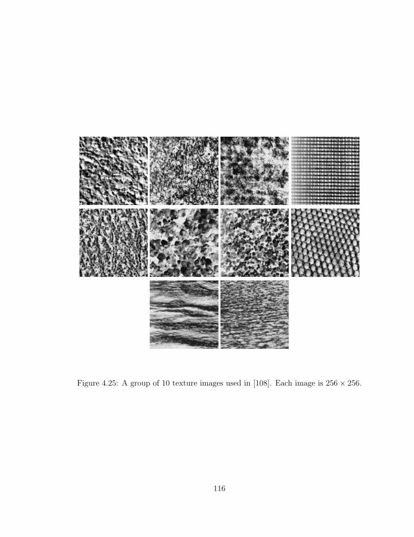
Figure 4.25: A group of 10 texture images used in [108]. Each image is 256× 256.

116

Figure 4.26: A group of 10 texture images used in [108]. Each image is 256× 256.

117

For content-based image retrieval, we use a database consisting of 100 texture

images each of which is composed of five texture regions from the texture image

database used in the classification example. For a given image patch, we extract

its spectral histogram as its footprint. As mentioned before, the same filters for

classification are used. Then we try to identify the best match in a texture image in

the database. To save some computation, we only compute spectral histogram on a

coarsely sampled grid.

Figure 4.27 shows an example. Figure 4.27(a) shows an input image patch with

size of 35× 35 in pixels. Figure 4.27(b) shows the minimum divergence between the

given patch and the images in the database. It shows clearly that there is a step edge.

The images that have a smaller matched error than the threshold given by the step

edge all actually contain the input match. Figure 4.27(c) shows the first nine image

with the matched error. The matched errors of the first eight images are much smaller

than the ninth image. This demonstrates that the spectral histogram characterizes

texture appearance very well for homogeneous textures.

Figure 4.28 shows another example. Here the texture is not very homogeneous

and consists of regular texture patterns. Figure 4.28(a) shows the input image patch

with size of 53 × 53 in pixels. Figure 4.28(b) shows the matched error of the 100

images in the database. While the edge is not a step edge, a ramp edge can be seen

clearly. As in Figure 4.27, this ramp edge defines a threshold for image that actually

contain patches that are perceptually similar to the given patch. Figure 4.28(c) shows

the first 12 images with the smallest match errors. All of them are correctly retrieved.

From these two examples, we can see a fixed threshold might be chosen. In both

cases, the threshold is around 0.25. Because χ2-statistic obeys a χ2 distribution, a

118

��0

10

20

30

40

50

60

70

80

90

10

00 1 2 3 4 5 6 7

(a)

(b)

0.0

73306

0.0

88377

0.0

91331

0.0

92707

0.0

92707

0.1

16957

0.2

53079

0.2

57533

2.4

76219

Figu

re4.27:

Image

retrievalresu

ltfrom

a100-im

agedatab

aseusin

ga

givenim

agepatch

based

onsp

ectralhistogram

s.(a)

Input

image

patch

with

size35×

35.(b

)T

he

sortedm

atched

errorfor

the

100im

agesin

the

datab

ase.(c)

The

first

nin

eim

agew

ithsm

allesterrors.

119

��

0 10 20 30 40 50 60 70 80 90 1000

0.5

1

1.5

2

2.5

3

3.5

4

4.5

(a) (b)

0.053618 0.068854 0.098365 0.098365

0.131868 0.138115 0.140837 0.141649

0.149421 0.175323 0.175323 0.210802

Figure 4.28: Image retrieval result from a 100-image database using a given imagepatch based on spectral histograms. (a) Input image patch with size 53×53. (b) Thesorted matched error for the 100 images in the database. (c) The first nine imagewith smallest errors.

120

threshold can be computed given a level of confidence. Also the algorithm is intrin-

sically parallel and local. Using parallel machines, the search may be implemented

very efficiently.

4.6 Comparison of Statistic Features

In this section, we numerically evaluate the performance of classification of differ-

ent features, different filters, and different distance measures for spectral histograms.

First we compare the spectral histogram with statistical values such as mean

and variance. If we assume that the underlying true image is a constant image, the

mean value is the best choice for a statistic feature. If we use a Gaussian model to

characterize the input image, mean and variance values are the features to be used.

Here we use a linear combination of mean and variance values, where the weights

are determined for the best performance at integration scale 35 × 35. We also use

the intensity histogram of image patches as a feature vector. Figure 4.29 shows the

classification error of the database used in Section 4 with respect to the integration

scale.

From Figure 4.29, we see that as the model gets more sophisticated, the perfor-

mance gets better. The mean value of each image patch does not provide a sufficient

feature for texture images and gives the largest classification error at all integration

scales. While the performance improves when the scale increases, the improvement

is not significant. Also the combination of mean and variance does not give good

results, suggesting Gaussian model, even though it is widely used in the literature, is

not good enough even for homogeneous texture images. The spectral histogram gives

the best performance at all integration scales. Compared with mean and Gaussian

121

0 20 40 60 80 100 1200

10

20

30

40

50

60

70

80

90

100

Figure 4.29: Classification error in percentage of texture database for different fea-tures. Solid line: spectral histogram of eight filters including intensity, gradients, LoGwith two scales and Gabor with three different orientations. Dotted line: Mean valueof the image patch. Dashed line: Weighted sum of mean and variance values of theimage patch. The weights are determined to achieve the best result for window size35× 35. Dash-dotted line: Intensity histogram of image patches.

model, the intensity histogram gives much better performance. This indicates that

the distribution is more important for texture discrimination and classification.

Ojala et al [99] did a comparison of different statistic features for texture image

classification using a database consisting of nine images only. Here we compare the

spectral histogram with gradient detectors, edge detectors (LoG) with different scales,

and Gabor filters with different scales and orientations. Figure 4.30 shows the result.

Compared to Figure 4.29, the differences between different feature detectors are not

large. At large integration scales, Gabor filters gives the second best result, suggesting

that oriented structures are more important for large texture patches than symmetric

edge detectors. Because gradient detectors are very local, they give the worst per-

formance. But if compared with the intensity histogram and Gaussian model shown

122

0 20 40 60 80 100 1200

10

20

30

40

50

60

70

80

Figure 4.30: Classification error in percentage of the texture database for differentfilters. Solid line: spectral histogram of eight filters including intensity, gradients,LoG with two scales and Gabor with three different orientations. Dotted line: Gra-dient filters Dxx and Dyy; Dashed line: Laplacian of Gaussian filters LoG(

√2/2),

LoG(1), and LoG(2). Dash-dotted line: Six Cosine Gabor filters with T = 4 and sixorientations θ = 0◦, 30◦, 60◦, 90◦, 120◦, and 150◦.

in Figure 4.29, it still gives a very good performance. This again confirms that the

distribution of local features is important for texture classification and segmentation.

Finally, for spectral histograms, we compare different distance measures. As given

in equations (4.4) (4.5), and (4.6), here we use L1-norm, L2-norm, Kullback-Leibler

divergence, and χ2-statistic. As shown in Figure 4.31, the differences between different

distance measures are very small, suggesting that spectral histograms do not depend

on the particular form of distance measure. This observation is different from the

conclusion in [107], where the authors claim χ2-statistic consistently gives the best

performance. The reason for the differences is that spectral histograms in our case are

derived by integrating information from the same window at different scales, while

different windows are used in [107] at different scales.

123

0 20 40 60 80 100 1200

10

20

30

40

50

60

70

Figure 4.31: Classification error in percentage of the texture database for differentdistance measures. Solid line: χ2-square statistic. Dotted line: L1-norm. Dashedline: L2-norm. Dash-dotted line: Kullback-Leibler divergence.

4.7 A Model for Texture Discrimination

In this section we apply our model to texture discrimination which is widely

studied in psychophysical experiments [69] using synthetic texton patterns. These

texton patterns are in general not homogeneous even within one texture region, for

example, as those shown in Figure 4.32. Our model is intended to characterize texture

regions with homogeneous appearance and thus the texton patterns do not fit to our

assumptions well. However, the result from our model is consistent with existing

psychophysical data and the data from the model by Malik and Perona [87].

We adopt similar procedures used by Malik and Perona [87]. Instead of using

192 filter pairs, we use two gradient filters Dxx and Dyy, three LoG filters with T

=√

2/2, 1, and 2, resulting in total of five filters. At each pixel, we extract local

spectral histograms at integration scale 29 × 29 and the gradient is the χ2-square

124

(+ O) (+ []) (L +) (L M)

(∆ →) (+ T) (+ X) (T L)

(LL ML) (R-mirror-R)

Figure 4.32: Ten synthetic texture pairs scanned from Malik and Perona [87]. Thesize is 136× 136.

distance between the spectral histograms of the two adjacent windows. Then the

gradient is averaged along each column.

The images used in our experiment are shown in Figure 4.32, which were scanned

from Malik and Perona [87]. The texture gradients for selected texture pairs (+ O)

and (R-mirror-R) from our method are shown in Figure 4.33 (b) and (d).

There are several observations that can be made from the gradient results shown

in Figure 4.33. First, the texture pattern does not give rise to a homogeneous texture

125

20 30 40 50 60 70 80 90 100 1100

20

40

60

80

100

120

(a) (b)

20 30 40 50 60 70 80 90 100 1100

5

10

15

(c) (d)

Figure 4.33: The averaged texture gradient for selected texture pairs. (a) The texturepair (+ O) as shown in Figure 4.32. (b) The texture gradient averaged along eachcolumn for (a). The horizontal axis is the column number and the vertical axis is thegradient. (c) The texture pair (R-mirror-R). (d) The averaged texture gradient for(c).

126

region, and variations within each texture region are clearly perceivable. For example,

in the texture pair (+ O), we do perceive columnar structures besides the major

texture boundary. Second, because of the inhomogeneity, the absolute value of texture

gradient should not be used directly as a measure for texture discrimination, which

was actually used by Malik and Perona [87]. As shown in Figure 4.33 (d), even though

the gradient is much weaker compared to Figure 4.33 (b), the filters still respond to

the texture variations, which is evident in Malik and Perona [87] also. However, the

texture boundary is not perceived.

Based on the above observations, we propose a texture discrimination measure as

the difference between the central peak and the maximum of adjacent side peaks. In

the (+ o) case, the central peak is 104.2320, and the left and right side peaks are

45.4100 and 34.6510 respectively, thus the discrimination measure is 58.8220. For the

(R-mirror-R) case, the central peak is 7.2310 and the left and right side peaks are

5.3580 and 11.4680 respectively, thus the measure is -4.2370, which indicates that the

two texture regions are not discriminable at all.

We calculate the proposed discrimination measure for the ten texture pairs. Table

4.3 shows the psychophysical data from [69], the data from Malik and Perona’s model

[87], and the proposed measure. Here the data from [69] was actually based on the

converted data shown in [87]. Figure 4.34 shows the data which are linearly scaled

so that the measures for (+ []) match. It is clear that our measure is consistent

with the other two except for the texture pair (L +). Our measure indicates that

that (+ O) is much easier to discriminate than the other pairs, the pair (LL, ML)

is barely discriminable with a measure of 0.2080, and the pair (R-mirror-R) is not

discriminable with a measure of -4.2370.

127

Texture discriminabilityTexture pair Data [69] Data [87] Our data

(+ o) 100 (saturated) 207 58.822(+ []) 88.1 225 15.518(L +) 68.6 203 6.657(L M) not available 165 10.008(∆ →) 52.3 159 7.8380(+ T) 37.6 120 6.6700(+ X) 30.3 104 6.0040(T L) 30.6 90 1.5390

(LL, ML) not available 85 0.208(R-mirror-R) not available 50 -4.237

Table 4.3: Comparison of texture discrimination measures

1 2 3 4 5 6 7 8 9 10−10

0

10

20

30

40

50

60

Figure 4.34: Comparison of texture discrimination measures. Dashed line - Psy-chophysical data from Krose [69]; dotted line - Prediction of Malik and Perona’s model[87]; solid line - prediction of the proposed model based on spectral histograms.

128

The proposed texture discrimination measure provides a potential advantage over

Malik and Perona’s model [87]. While their model cannot account for asymmetry

[140] which exists in human texture perception, our model can potentially account for

that. In general, the discrimination of a more variant texture in a field of more regular

texture is stronger than vice versa. For example, the perception of gapped circles in

a field of closed circles is stronger than the perception of closed circles in a field of

gapped circles [140]. According to our discrimination measure, the asymmetry is due

to that the side peak of a regular texture is weaker than the side peak of a variant

texture, resulting in stronger discrimination. This needs to be further investigated.

4.8 Conclusions

In this chapter, we propose spectral histograms as a generic feature vector for natu-

ral images and a similarity measure is defined. This provides a generic non-parametric

similarity measure for images. We demonstrate the texture characterization and dis-

crimination capabilities of spectral histograms using image synthesis, classification,

content-based image retrieval, and texture discrimination. As shown in Figure 4.30,

we demonstrate that particular forms of filters are not important, but the distribu-

tions are critical. We also demonstrate that the performance of spectral histograms

largely do not depend on the particular form of the distance measure. We show the

spectral histogram gives much better performance than simple statistic features such

as variance and mean values.

The classification and other results would be improved even significantly if more

sophisticated algorithms for similarity measure and classification would be used.

The distance measures defined in equations (4.4) (4.5), and (4.6) are simply equally

129

weighted summations from all the histogram bins. If many samples are available for

one texture type, homogeneity of the texture can be refined using different weights for

different filters and even bins. Those weights can be learned from training samples,

as demonstrated by Zhu et al [149].

While spectral histograms can capture inhomogeneity of texture images, as shown

in texture synthesis examples, they are not able to capture the geometric relationships

among texture elements if spatially the relationships are longer than the filters used.

Modeling the geometric relationships may even be more salient for certain textures

such as textures consisting of regular patterns of similar elements. A level beyond

this filtering needs to be incorporated or a different module might be needed. One

possible way is to allow short-range coupling instead of nearest-neighbor coupling to

overcome the inhomogeneity present in the image. Those issues need to be further

investigated.

130

Documents

CHAPTER 4 SPECTRAL HISTOGRAM: A GENERIC FEATURE FOR …fsvision.fsu.edu/publications/papers/dissertation/chapter04.pdf · histogram for each local window in the pyramid. We obtain