Embed Size (px)
Citation preview

Chapter 4: Regression With One Regressor
Copyright © 2011 Pearson Addison-Wesley. All rights reserved. 1-1

Outline
1. Fitting a line to data
2. The ordinary least squares (OLS) line/regression
3. Measures of fit
Copyright © 2011 Pearson Addison-Wesley. All rights reserved.
3. Measures of fit
4. Population model
5. The least squares assumptions
6. The sampling distribution of the OLS estimator4-2

Fitting a line to data
• Suppose data on two rvs (X,Y): (X1,Y1), …, (Xn,Yn)
No probability distribution for now
• Suspect Y depends somewhat on X, e.g.
Yi = average test score in school district i
Copyright © 2011 Pearson Addison-Wesley. All rights reserved.
i
Xi = average student-teacher ratio in school district i
• Try to summarize/fit this dependence (if any) by a line
defined by the intercept, slope parameters: b0, b1
Seek b0, b1 s.t. data approximately satisfy:
Known as a regression.
1-3
0 1i iY b b X≈ +

Residuals of a particular line β0,β1
Copyright © 2011 Pearson Addison-Wesley. All rights reserved. 4-4

Errors/residuals in fit
• Given a line b0,b1, define errors/residuals as
• Wish ui=1,…,n to be “zeroish”. This wish can be interpreted as a specific goal in various ways.
0 1 0 1: ( ) s o i i i i i iu Y b b X Y b b X u= − + = + +
Copyright © 2011 Pearson Addison-Wesley. All rights reserved.
i=1,…,n
a specific goal in various ways.
• One is in terms of the sum of squared residuals:
• So the goal is to choose the line b0,b1 to minimize SSR
The minimands b*0,b*1 are known as “least squares”
• We will see another way later
1-5
2
1,...,
:i
i n
SSR u=
= ∑

Least squares
• So the least squares b*0,b*1 minimize this
• If you know basic calculus, you can set equal to zero the derivative of SSR wrt b , and that of SSR wrt b .
2 2
0 1(Y b X )i i i
SSR u b= = − −∑ ∑
Copyright © 2011 Pearson Addison-Wesley. All rights reserved.
derivative of SSR wrt b0 , and that of SSR wrt b1.
Then solve the system of two equations for unknowns b0,b1
• Fitted/estimated/”predicted” value:
Residual/error:
• Following is the least squares line b*0, b*1 :
1-6
�
�
* *
0 1:
:
i i
ii i
Y b b X
u Y Y
= +
= −�
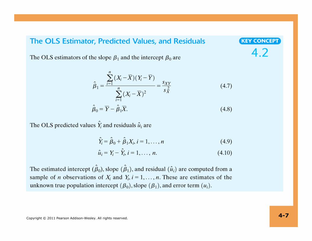
Copyright © 2011 Pearson Addison-Wesley. All rights reserved. 4-7
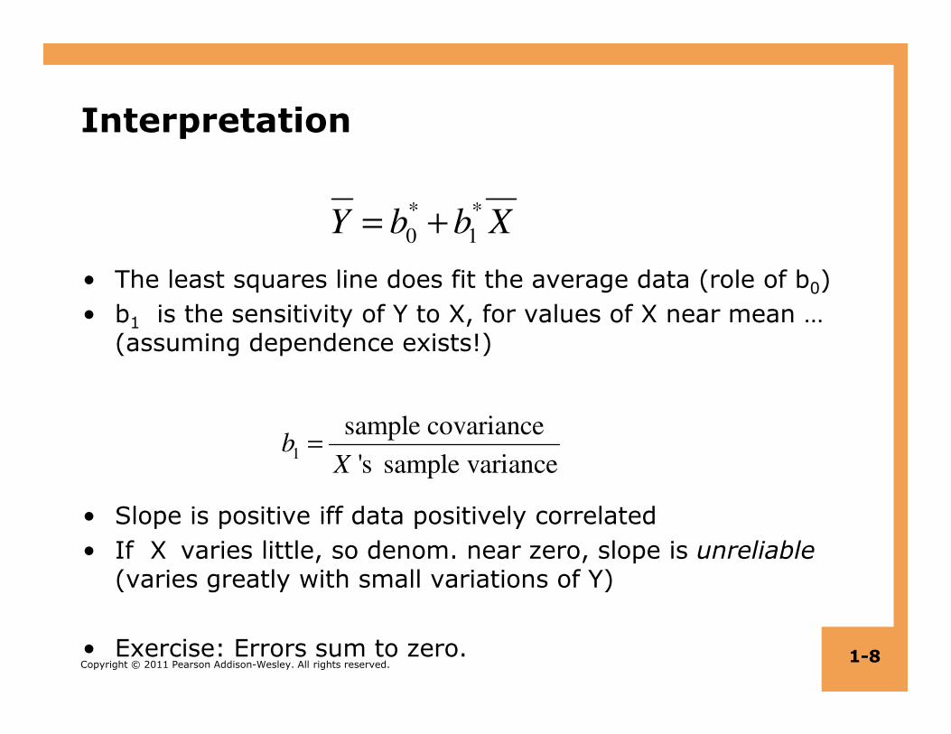
Interpretation
• The least squares line does fit the average data (role of b0)
• b1 is the sensitivity of Y to X, for values of X near mean … (assuming dependence exists!)
* *
0 1Y b b X= +
Copyright © 2011 Pearson Addison-Wesley. All rights reserved.
• Slope is positive iff data positively correlated
• If X varies little, so denom. near zero, slope is unreliable(varies greatly with small variations of Y)
• Exercise: Errors sum to zero. 1-8
1
sample covariance
's sample varianceb
X=

Application to CA data
Copyright © 2011 Pearson Addison-Wesley. All rights reserved.
• Slope = = – 2.28
• Intercept = = 698.9
• Least squares line: = 698.9 – 2.28×STR
4-9
�TestScore

Fitted value X residual
Copyright © 2011 Pearson Addison-Wesley. All rights reserved.
For i =Antelope, CA district, (Xi,Yi)=(19.33,657.8)
fitted value: = 698.9 – 2.28×19.33 = 654.8
residual: = 657.8 – 654.8 = 3.0 4-10
ˆAntelope
Y
ˆAntelope
u

Interpretation here
� 689.9 2.28TestSco Sre TR= − ×
• Districts with one fewer student per teacher have average test scores 2.28 points higher, on average
• Do not interpret the intercept as the value of the line at X=0
Copyright © 2011 Pearson Addison-Wesley. All rights reserved. 4-11
• Do not interpret the intercept as the value of the line at X=0
• For there are no school districts with every classroom empty (STR=X=0), and, even if there were, there would be no test scores in such classrooms (i.e. Y’s)
• The intercept is just something that makes this true:
0 1Y b b X= +
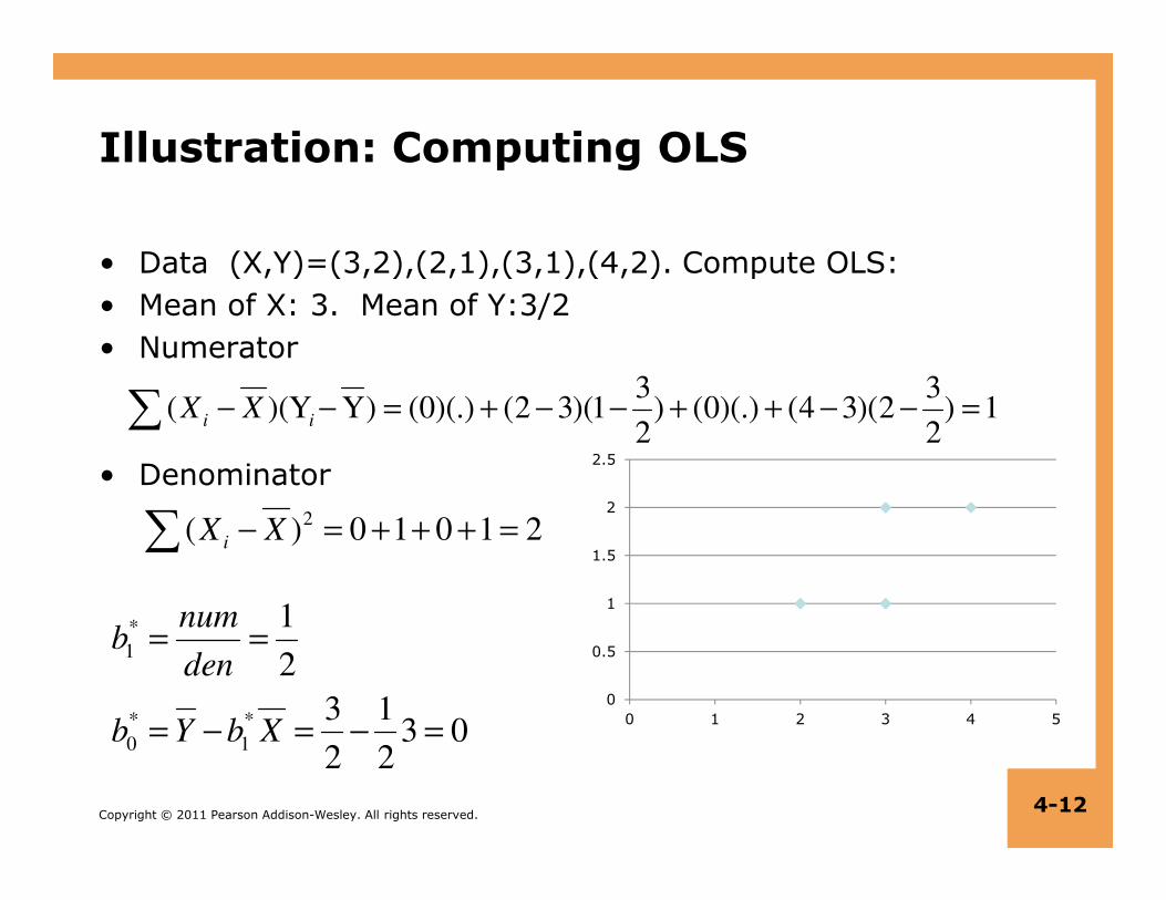
Illustration: Computing OLS
• Data (X,Y)=(3,2),(2,1),(3,1),(4,2). Compute OLS:
• Mean of X: 3. Mean of Y:3/2
• Numerator
3 3( )(Y Y) (0)(.) (2 3)(1 ) (0)(.) (4 3)(2 ) 1
2 2i i
X X− − = + − − + + − − =∑
Copyright © 2011 Pearson Addison-Wesley. All rights reserved.
• Denominator
4-12
2( ) 0 1 0 1 2iX X− = + + + =∑
*
1
* *
0 1
1
2
3 13 0
2 2
numb
den
b Y b X
= =
= − = − =0
0.5
1
1.5
2
2.5
0 1 2 3 4 5

Measures of Fit
There are two measures of the fit of the line to the data:
• The R2 measures the fraction of the variance of Y that is explained by X.
Copyright © 2011 Pearson Addison-Wesley. All rights reserved.
• The standard error of the regression (SER) measures the magnitude of the regression’s errors.
4-13

The R2
• Recall, from def. of u. Exercise:
So
Variance splits into “explained” and “unexplained” parts
• Dividing,
� �i i i
Y Y u= + � �cov( , ) 0i iY u =� �var( ) var( ) var ( )
i i iY Y u= +
� �var( ) var ( )1
var( ) var( )
i iY u
Y Y= +
Copyright © 2011 Pearson Addison-Wesley. All rights reserved.
… the “explained” and “unexplained” proportions of var(Y)
This explained proportion is called 0 ≤ R2 ≤ 1.
• Often worded via TSS:= ∑(Yi-Y*)2 and (minimized) SSR:
4-14
1var( ) var( )i iY Y
= +
� � 2
2
2
(u 0)var(u )1 1 1
var( ) ( )
ii
i i
SSRR
Y TSSY Y
−= − = − = −
−
∑∑

The R2 – cont’d
• Often worded via ESS:=∑(Yihat-Y*)2.
2
2
2
ˆˆ ( )var( ):
var( ) ( )
ii
i i
Y YY ESSR
Y Y Y TSS
−= = =
−
∑∑
Copyright © 2011 Pearson Addison-Wesley. All rights reserved.
• Whatever formula one uses, clearly higher R2 is better.
• Exercise: R2 = the square of the correlation b/w X,Y
4-15
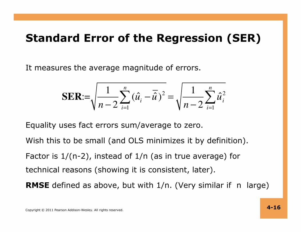
It measures the average magnitude of errors.
Standard Error of the Regression (SER)
2 2
1 1
1 1ˆ ˆ ˆ:= ( )
2 2
n n
i i
i i
u u un n= =
− =− −∑ ∑SER
Copyright © 2011 Pearson Addison-Wesley. All rights reserved. 4-16
Equality uses fact errors sum/average to zero.
Wish this to be small (and OLS minimizes it by definition).
Factor is 1/(n-2), instead of 1/n (as in true average) for
technical reasons (showing it is consistent, later).
RMSE defined as above, but with 1/n. (Very similar if n large)

R2 & SER for CA data
Copyright © 2011 Pearson Addison-Wesley. All rights reserved.
R2 = .05, SER = 18.6 … poor fit
X=STR explains via Yhat only a small fraction of var(test scores)
4-17

The Linear Regression Model
So far, given data, discussed how to fit line and measure fit.
Discussion apart of any probabilistic model for data. Now:
Assume Yi = β0 + β1Xi + ui i = 1,…, n
Copyright © 2011 Pearson Addison-Wesley. All rights reserved.
• Data generated as follows:
• The X’s: Given.
• The Y’s: There are constants β0,β1 & rv u (“error term”) such that every observed Yi arises linearly as above.
• X is known as the independent variable or regressor
• Y as the dependent variable
• Error term subsumes “omitted factors” & “data measurement errors”.
4-18

Purpose of the Linear Regression Model
• The assumption implies that there is some true model generating the data & OLS b’s.
• The CLT will imply, given conditions, the rate at which the average data & the OLS b’s converge to the true model.
Copyright © 2011 Pearson Addison-Wesley. All rights reserved.
• Note: Without a true model, what is there to converge to?!
• The OLS b’s are called estimates (of the true β0,β1).
• (This usage senseless without the data-generating model.)
• As in ch3, we will address whether E(b)= β (unbiased), b->β (consistency), & rate of convergence/confidence intervals
4-19
� �0 1,β β

The OLS Assumptions
Assume Yi = β0 + β1Xi + ui i =1,…,n
1. Error term conditional on X has mean zero, E(u|X=x)
2. (Xi,Yi)i =1,…,n, are i.i.d.
Copyright © 2011 Pearson Addison-Wesley. All rights reserved.
i i i =1,…,n
3. Outliers are rare: E(X4), E(Y4) are finite.
Purpose:
• (1) implies is unbiased.
• (2) implies sampling distribution of ; true under SRS
• (3) needed to apply CLT for confidence intervals
4-20
� �0 1,β β

OLS assumption 1: E(u|X = x) = 0
Copyright © 2011 Pearson Addison-Wesley. All rights reserved.
• Example: E(u|STR=16)=0
• What are some of these “other factors”? District’s wealth, parental involvement, … across all districts with STR=16,
these factors average out, says the assumption
• Note, STR=16 is low, so those districts tend to be wealthy already, suggesting in fact E(u|STR=16)>0 for such rvs.
• Exercise: Ass’n implies cov(Xi,ui)=0
4-21

OLS assumption 2: (Xi,Yi)i = 1,…,n are iid
True if entity (individual, district) is simply randomly sampled:
• The entities are selected from the same population, so (Xi, Yi) are identically distributed for all i = 1,…, n.
• The entities are selected at random, so the values of (X, Y) for different entities are independently distributed.
Copyright © 2011 Pearson Addison-Wesley. All rights reserved.
different entities are independently distributed.
One case where sampling is not-iid is where data for the same entity are recorded over time (panel & time series data)
Entity’s data tends to show time-dependence (not independent) Eg district with small STR in 1999 is likely to have small STR in 2000. We’ll address time later in course.
4-22

OLS assumption 3: E(X4) & E(Y4) finite
• Says extreme outliers are rare
• This true whenever both X,Y are bounded. Eg, in CA data, X=STR is bounded between 0 and lawful maximum (100?)
Y=test score bounded between 0 and test max (1600?)
Copyright © 2011 Pearson Addison-Wesley. All rights reserved.
• Adding a large outlier drastically changes OLS estimate (since largeness in squared in errors), so this assumption says that data averages are stable as sample grows
• Btw, look in data for outliers that may be justifiable removed, eg wrong code, scale, unit.
4-23

Why ass’n 3 important
Copyright © 2011 Pearson Addison-Wesley. All rights reserved.
• Black dots get OLS line that is flat
• Adding one red outlier, though one among many points, causes OLS line to move drastically
• OLS unreliable if, as sample grows, reds arise often4-24

Sampling Distribution of OLS Estimator
The OLS estimate is defined by a sample of data. Different
samples yield different estimates. So OLS estimate is a rv.
Copyright © 2011 Pearson Addison-Wesley. All rights reserved.
Wish to learn its sampling distribution. This so as to:
• Test hypotheses such as β1 = 0
• Construct confidence intervals for β1
Analogous to what we did with the sample mean as an estimate rv of the true mean
4-25

Key auxiliary fact:
• Result: OLS unbiased, E(β1hat)=β1
Proof: Suffices that E(fraction)=0. Toward this, use Law of Iterated Expectations E(rv)=E[E(rv|X)]:
�1 1 2
( ) = error term
( )
i i
i
i
X X uu
X Xβ β
−= +
−
∑∑
1,...,( ) ( ) E[ | ] ( )0= = 0
i i i i i n iX X u X X u X X X
E E E=
− − −=
∑ ∑ ∑
Copyright © 2011 Pearson Addison-Wesley. All rights reserved.
• Detail:
-Used E[ui|Xi=1,…,n] = E[ui|Xi] since independently dist’d
-In turn used E[ui|Xi] = 0 since assn 2
-So E[ui|Xi=1,…,n] = 0 in the above
4-26
1,...,
2 2 2
( ) ( ) E[ | ] ( )0= = 0
( ) ( ) ( )
i i i i i n i
i i i
X X u X X u X X XE E E
X X X X X X
= − − −
= − − −
∑ ∑ ∑∑ ∑ ∑
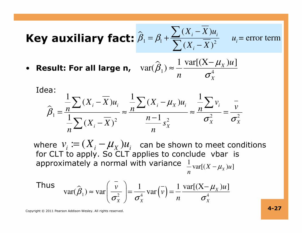
Key auxiliary fact:
• Result: For all large n,
Idea:
�1 1 2
( ) = error term
( )
i i
i
i
X X uu
X Xβ β
−= +
−
∑∑
�1 2 2
1 1 1( ) ( )
1 1
i i i X i iX X u X u vvn n n
n
µβ
σ σ
− −= ≈ ≈ =
−
∑ ∑ ∑
∑
�1 4
var[(X ) ]1var( ) X
X
u
n
µβ
σ
−≈
Copyright © 2011 Pearson Addison-Wesley. All rights reserved.
where can be shown to meet conditions for CLT to apply. So CLT applies to conclude vbar is approximately a normal with variance
Thus
4-27
1 2 22 21 1
( ) X Xi X
nX X s
n n
σ σ−−∑
: ( )i i X i
v X uµ= −
1var[( ) ]
XX u
nµ−
� ( )1 2 4 4
var[(X ) ]1 1var( ) var var X
X X X
uvv
n
µβ
σ σ σ
−≈ = =
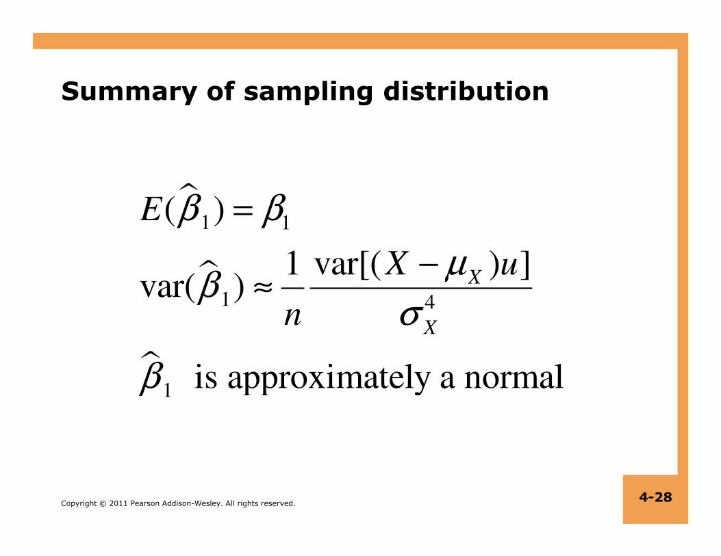
Summary of sampling distribution
�
�
1 1( )
var[( ) ]1var( ) X
E
X u
β β
µβ
=
−≈
Copyright © 2011 Pearson Addison-Wesley. All rights reserved. 4-28
�
�
1 4
1
var[( ) ]1var( )
is approximately a normal
X
X
X u
n
µβ
σ
β
−≈

Importance of var(X) for reliability of OLS
Note, we see var( ) is inversely proportional to
So the greater var(X), the more reliable is estimate
More information in the data makes slope easy to ascertain
4
Xσ
Copyright © 2011 Pearson Addison-Wesley. All rights reserved.
Illustration
#blue dots = #black dots
Slope for blues? Unsure…
Slope for blacks? About 2!
Difference is that blacks got
greater spread, variance.
4-29

Copyright © 2011 Pearson Addison-Wesley. All rights reserved. 4-30

Appendix I:
• Let us show this auxiliary result that lead to our key results
Averaging model Yi = β0 + β1Xi + ui and then subtracting,
Let us substitute this in the OLS formula for β1:
�1 1 2
( ) = error term
( )
i i
i
i
X X uu
X Xβ β
−= +
−
∑∑
0 1 1 Y ( ) ( )i i iY X u Y X X u uβ β β= + + → − = − + −
Copyright © 2011 Pearson Addison-Wesley. All rights reserved.
1
4-31
� 1
1 2 2
1 2 2
1 2 2
(X ) ( u) (X )(Y Y)(X )
(X ) (X )
(X )(X ) ( u)(X )
(X ) (X )
(X ) 0(X )u
(X ) (X )
i i ii i
i i
i i i i
i i
ii i
i i
X u XX
X X
X X u X
X X
Xu X
X X
ββ
β
β
− + − −− − = =− −
− − − −= +
− −
− =−= + −
− −
∑∑∑ ∑
∑ ∑∑ ∑
∑∑∑ ∑

Appendix II: Derivation of OLS estimates
• Recall definition of residual ui := Yi – (b0 + b1Xi) and of criterion SSR :=∑ ui
2 that OLS b0,b1 are to minimize.
To compute these, take derivatives wrt them and set to 0:
0 10
( ) (Y (b b X )) 0 2 2 2i i i
i i i
d u ddb SSR u u u
db db db
− += = = = −∑ ∑ ∑
Copyright © 2011 Pearson Addison-Wesley. All rights reserved.
This is asking that residuals add (or average) to zero, i.e. that
4-32
0 0 0db db db∑ ∑ ∑
*
0 1 0 10 (b b X) b b Xu Y Y= = − + → = −
0 11
1 1 1
2
0 1 0 1
( ) (Y (b b X )) 0 2 2 2 X
That is, 0 (Y (b b X )) X Y X b b
i i ii i i i
i i i i i i
d u ddb SSR u u u
db db db
nX X
− += = = = −
= − + = − +
∑ ∑ ∑
∑ ∑ ∑

Appendix II: cont’d
Substituting b0,
( )
2
1 1
22
1
*
1 22
0 Y X (Y b X) b
Y X Y
Y X Y
i i i
i i i
i i
nX X
nX b X nX
nXb
X nX
= − − +
− = −
−=
−
∑ ∑
∑ ∑
∑∑
Copyright © 2011 Pearson Addison-Wesley. All rights reserved.
Now, a bit of algebra show the numerator is
denominator is
(Just expand the latter, simplify, and get the above fraction.)
Finally, these are global minima (vs. local minima or maxima) because the derivative of prior derivatives is positive.
4-33
2
iX nX−∑
( )( )i iY Y X X− −∑2
( )iX X−∑