Embed Size (px)
Citation preview

The Islamic University of GazaFaculty of Engineering
Civil Engineering Department
Numerical AnalysisECIV 3306
Chapter 31: Finite-Element Method
Finite-Element Method
• Finite element method provides an alternative tofinite-difference methods, especially for systems withirregular geometry, unusual boundary conditions, orheterogeneous composition.
• Advantages:
• Flexibility with respect to boundary conditions andgeometries.
2Chapter 31

Finite-Element Method
• This method divides the solution domain into simplyshaped regions or elements. An approximate solutionfor the PDE can be developed for each element.
• The total solution is generated by linking together, or“assembling,” the individual solutions taking care toensure continuity at the inter-element boundaries.
3Chapter 31

Figure 31.1
Chapter 31 4

Finite-Element Method
• A comprehensive description of finite elementmethod is beyond the scope of this course.
• This chapter provides a general introduction to themethod. Our primary objective is to make youcomfortable with the approach and cognizant of itscapabilities.
5Chapter 31
The General Approach
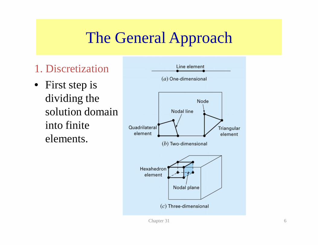
1. Discretization• First step is
dividing thesolution domaininto finiteelements.
Chapter 31 6
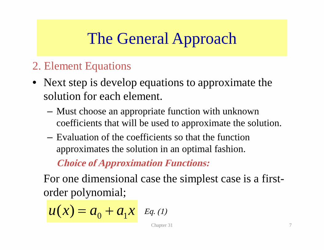
2. Element Equations• Next step is develop equations to approximate the
solution for each element.– Must choose an appropriate function with unknown
coefficients that will be used to approximate the solution.– Evaluation of the coefficients so that the function
approximates the solution in an optimal fashion.Choice of Approximation Functions:
For one dimensional case the simplest case is a first-order polynomial;
xaaxu 10)( +=Chapter 31 7
The General Approach
Eq. (1)

12
12
12
21
2211
12
121
12
12210
222102
111101)(
)(
xxxxN
xxxxN
uNuNu
-xx-uua
-xxx-uxua
xuuxaauxuuxaau
--
=--
=
+=
==
=+==+=
8
Approximation orshape function
Interpolation functions
Solve for a0 and a1
Substitute in u(x)
The General Approach
Eq. (2)
Chapter 31

• The fact that we are dealing with linear equations facilitatesoperations such as differentiation and integration:
Obtaining an Optimal Fit of the Function to the Solution:• Most common approaches are the direct approach, the method
of weighted residuals, and the variational approach.
( ) )(2
)(12
212211
12
122
21
1
2
1
2
1
xxuudxuNuNdxu
andxxuuu
dxdNu
dxdN
dxdu
x
x
x
x
-+
=+=
--
=+=
òò
Chapter 31 9
The General Approach
Eq. (3)
Eq. (4)

• Mathematically, the resulting element equations willoften consists of a set of linear algebraic equationsthat can be expressed in matrix form:
[k]=an element property or stiffness matrix{u}=a column vector of unknowns at the nodes{F}=a column vector reflecting the effect of anyexternal influences applied at the nodes.
[ ]{ } { }Fuk =
Chapter 31 10
The General Approach
Eq. (5)

Chapter 31 11
3.Assembly• The assembly process is governed by the concept of continuity.• The solutions for contiguous elements are matched so that the
unknown values (and sometimes the derivatives) at theircommon nodes are equivalent.
• When all the individual versions of the matrix equation arefinally assembled:
[K] = assemblage property matrix{u ´} and {F ´}= assemblage of the vectors {u } and {F }
[ ]{ } { }FuK ¢=¢
The General Approach
Eq. (6)

4. Boundary Conditions/• Matrix equation when modified to account for
system’s boundary conditions:
5. Solution/• In many cases the elements can be configured so that
the resulting equations are banded. Highly efficientsolution schemes are available for such systems (PartThree).
[ ]{ } { }Fuk ¢=¢
Chapter 31 12
The General Approach
Eq. (7)

6.Post-processing/• Upon obtaining solution, it can be displayed in
tabular form or graphically.
Chapter 31 13
The General Approach

Finite Element Application in onedimension
T=40 T=200=10
)(2
2xf
dxTd
-==10
Chapter 31 14
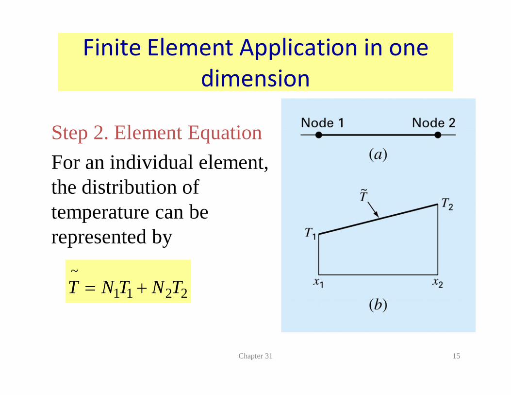
Step 2. Element EquationFor an individual element,the distribution oftemperature can berepresented by
Chapter 31 15
Finite Element Application in onedimension
2211~
TNTNT +=

Using The method of weighted residuals (MWR)to obtain an optimal fit of the function to thesolution.
Chapter 31 16
Finite Element Application in onedimension
òò +-=2
1
2
1
11
~1
~
)()(x
x
x
x
dxNxfdx
xTddxdx
dNdxTd
)(.
1).(
2112
212
211~
2
1
2
1
TTxx
dxxxTTdx
dxdN
dxTd
x
x
x
x
--
=-
-= òò
and
)(1).(
211.2
212
212~
2
1
2
1
TTxx
dxxxTTdx
dxdN
dxTd
x
x
x
x
+--
=-
+-= òò
But from Eq. (3)
and
òò +-=2
1
2
1
22
~2
~
)()(x
x
x
x
dxNxfdx
xTddxdx
dNdxTd Eq. (8)
….Eq. (9)

Representing Eq. (9) in matrix form;
Substituting this result into Eq. (8) and expressing theresult in matrix form gives the final version of theelement equations
17
Finite Element Application in onedimension
þýü
îíì
·úû
ùêë
é-
--
=
ïïï
þ
ïïï
ý
ü
ïïï
î
ïïï
í
ì
ò
ò
2
1
122
~
1~
11111
2
1
2
1
TT
xxdx
dxdN
dxTd
dxdx
dNdx
Td
x
x
x
x
ïïï
þ
ïïï
ý
ü
ïïï
î
ïïï
í
ì
+
ïïþ
ïïý
ü
ïïî
ïïí
ì-
=þýü
îíì
·úû
ùêë
é-
--
ò
ò2
1
2
1
2
1
2
1
2
1
12)(
)(
)(
)(
11111
x
x
x
x
dxNxf
dxNxf
dxxdT
dxxdT
TT
xx
Element stiffnessmatrix
Boundaryconditions
Externaleffects
Eq. (10)

Finite Element Application in onedimension Example
(10)
10(2)
10
þýü
îíì
+
ïïþ
ïïý
ü
ïïî
ïïí
ì-
=þýü
îíì
·úû
ùêë
é-
-5.125.12
)(
)(
4.04.04.04.0
2
1
2
1
dxxdT
dxxdT
TT
10

Step 3. Assembly• Before the element equations are assembled, a
global numbering scheme must be established.
Chapter 31 19
One dimension – Example- cont.
Element
Node number
Local Global
1 1 1
2 2
2 1 2
2 3
3 1 3
2 4
4 1 4
2 5
• For each element theelement equation can bewritten using the globalcoordinates. Then they canbe added one at a time toassemble the total systemmatrix.

Chapter 31 20
One dimension – Example- cont.
ïïï
þ
ïïï
ý
ü
ïïï
î
ïïï
í
ì++-
=
ïïï
þ
ïïï
ý
ü
ïïï
î
ïïï
í
ì
·
úúúúúú
û
ù
êêêêêê
ë
é-
-
000
5.12/)(5.12/)(
000
0000000000000000004.04.00004.04.0
)2
1
2
1dxxdTdxxdT
TT
a
ïïï
þ
ïïï
ý
ü
ïïï
î
ïïï
í
ì
++
+-
=
ïïï
þ
ïïï
ý
ü
ïïï
î
ïïï
í
ì
·
úúúúúú
û
ù
êêêêêê
ë
é
--+-
-
00
5.12/)(5.125.12
5.12/)(
00
0000000000004.04.000004.04.04.04.00004.04.0
) 3
1
3
2
1
dxxdT
dxxdT
TTT
b
ïïï
þ
ïïï
ý
ü
ïïï
î
ïïï
í
ì
++
+-
=
ïïï
þ
ïïï
ý
ü
ïïï
î
ïïï
í
ì
·
úúúúúú
û
ù
êêêêêê
ë
é
---
---
05.12/)(
5.125.1225
5.12/)(
00000004.04.000004.04.04.04.00004.08.04.00004.04.0
)
4
1
4
3
2
1
dxxdT
dxxdT
TTTT
c
ïïï
þ
ïïï
ý
ü
ïïï
î
ïïï
í
ì
++
+-
=
ïïï
þ
ïïï
ý
ü
ïïï
î
ïïï
í
ì
·
úúúúúú
û
ù
êêêêêê
ë
é
--+-
----
-
5.12/)(5.125.12
2525
5.12/)(
04.04.000004.04.04.04.000
04.08.04.00004.08.04.00004.04.0
)
4
1
4
3
2
1
dxxdT
dxxdT
TTTT
d
ïïï
þ
ïïï
ý
ü
ïïï
î
ïïï
í
ì
+
+-
=
ïïï
þ
ïïï
ý
ü
ïïï
î
ïïï
í
ì
·
úúúúúú
û
ù
êêêêêê
ë
é
---
----
-
5.12/)(252525
5.12/)(
4.04.00004.08.04.000
04.08.04.00004.08.04.00004.04.0
)
5
1
5
4
3
2
1
dxxdT
dxxdT
TTTTT
e
Final resultfor
[ ]{ } { }FuK ¢=¢
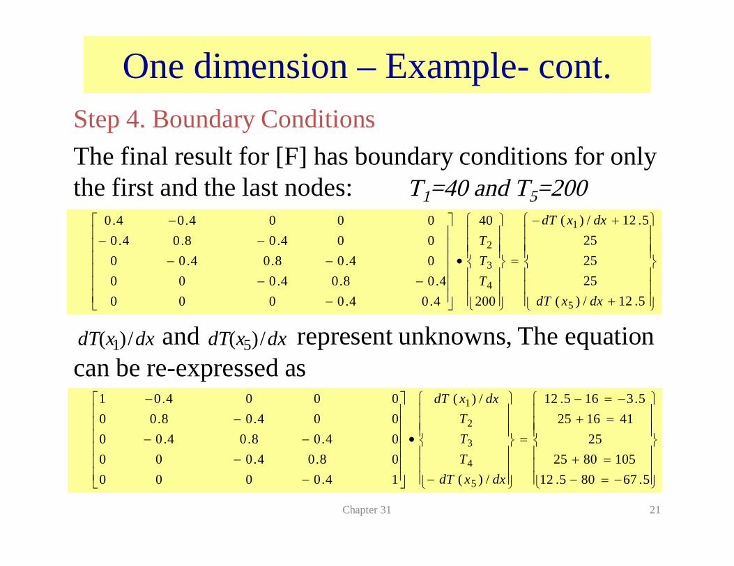
Step 4. Boundary ConditionsThe final result for [F] has boundary conditions for onlythe first and the last nodes: T1=40 and T5=200
and represent unknowns, The equationcan be re-expressed as
Chapter 31 21
One dimension – Example- cont.
ïïï
þ
ïïï
ý
ü
ïïï
î
ïïï
í
ì
+
+-
=
ïïï
þ
ïïï
ý
ü
ïïï
î
ïïï
í
ì
·
úúúúúú
û
ù
êêêêêê
ë
é
---
----
-
5.12/)(252525
5.12/)(
200
40
4.04.00004.08.04.000
04.08.04.00004.08.04.00004.04.0
5
1
4
3
2
dxxdT
dxxdT
TTT
dxxdT /)( 1 dxxdT /)( 5
ïïï
þ
ïïï
ý
ü
ïïï
î
ïïï
í
ì
-=-=+
=+-=-
=
ïïï
þ
ïïï
ý
ü
ïïï
î
ïïï
í
ì
-
·
úúúúúú
û
ù
êêêêêê
ë
é
--
---
-
5.67805.121058025
25411625
5.3165.12
/)(
/)(
14.000008.04.00004.08.04.00004.08.000004.01
5
4
3
2
1
dxxdTTTT
dxxdT

Step 5. SolutionSolve five unknowns
Chapter 31 22
One dimension – Example- cont.
ïïï
þ
ïïï
ý
ü
ïïï
î
ïïï
í
ì
-
=
ïïï
þ
ïïï
ý
ü
ïïï
î
ïïï
í
ì
3475.253
24575.173
66
/)(
/)(
5
4
3
2
1
dxxdTTTT
dxxdT

Step 6. Post-processing
Chapter 31 23
One dimension – Example- cont.

Step - 1;Discretization
Finite-element Solution of A Seriesof Springs Example 2
Using the step-by-step procedure a finite-elementapproach to determine the displacements of the springs.

Step 2. Element EquationThe relationship between force F and displacement xcan be represented mathematically by Hooke's law:
Chapter 31 25
Solution of A Series of SpringsExample 2 – cont.
kxF =For the shown spring
or
For a stationary system, F1 = -F2
)( 211 xxkF -=
211 kxkxF -=
212 kxkxF +-=

Step 2. Element EquationThese two simultaneous equations specify thebehavior of the element (spring). They can bewritten in matrix form as;
or
Chapter 31 26
Solution of A Series of SpringsExample 2 – cont.
þýü
îíì
=þýü
îíì
·úû
ùêë
é-
-
2
1
2
1FF
xx
kkkk
[ ]{ } { }Fuk = Eq. (5)

Step 3. Assembly• Established a global numbering
scheme.
Chapter 31 27
Solution of A Series of SpringsExample 2 – cont.
Element
Node numberLocal Global
1 1 12 2
2 1 22 3
3 1 32 4
4 1 42 5
ïþ
ïýü
ïî
ïíì
=þýü
îíì
·úúû
ù
êêë
é
-
-)(
2
)(1
2
1)(
22)(
21
)(12
)(11
e
e
ee
ee
FF
xx
kkkk
ïïï
þ
ïïï
ý
ü
ïïï
î
ïïï
í
ì
=
ïïï
þ
ïïï
ý
ü
ïïï
î
ïïï
í
ì
·
úúúúúúú
û
ù
êêêêêêê
ë
é
-
-+-
-+-
-+-
-
)4(2
)1(1
5
4
3
2
1
)4(22
)4(21
)4(12
)4(11
)3(22
)3(21
)3(12
)3(11
)2(22
)2(21
)2(11
)2(11
)1(22
)1(11
)2(12
)1(11
000
F
F
xxxxx
kkkkkk
kkkkkkkk
kk
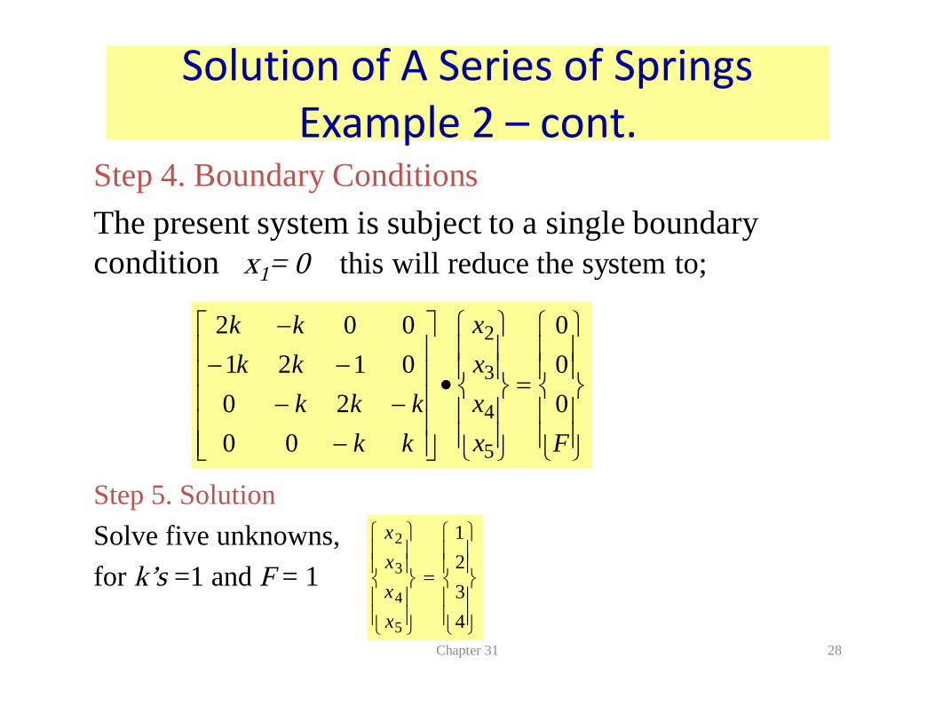
Step 4. Boundary ConditionsThe present system is subject to a single boundarycondition x1= 0 this will reduce the system to;
Step 5. SolutionSolve five unknowns,for k’s =1 and F = 1
Chapter 31 28
Solution of A Series of SpringsExample 2 – cont.
ïïþ
ïïý
ü
ïïî
ïïí
ì
=
ïïþ
ïïý
ü
ïïî
ïïí
ì
·
úúúúú
û
ù
êêêêê
ë
é
---
---
Fxxxx
kkkkk
kkkk
000
0020
0121002
5
4
3
2
ïïþ
ïïý
ü
ïïî
ïïí
ì
=
ïïþ
ïïý
ü
ïïî
ïïí
ì
4321
5
4
3
2
xxxx
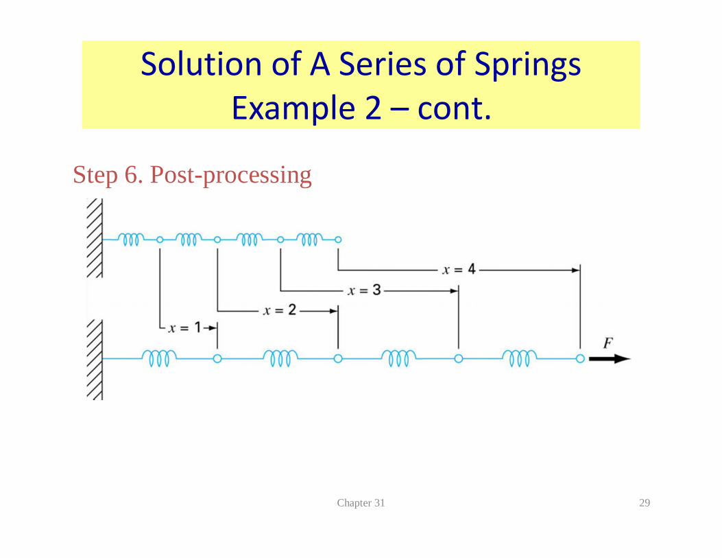
Step 6. Post-processing
Chapter 31 29
Solution of A Series of SpringsExample 2 – cont.

Perform the same computation for the series ofsprings example, but change the force F to 1.5and the spring constant to
Chapter 31 30
H.W
Spring 1 2 3 4
k 0.75 1.5 0.5 2


