Chapter 3 Electromagnetism and Gravitation in Various ...fma.if.usp.br/~amsilva/Livros/Zwiebach/chapter3.pdf · Chapter 3 Electromagnetism and Gravitation in Various Dimensions String

Chapter 3

Electromagnetism andGravitation in VariousDimensions

String theory is promising because it includes Maxwell electrodynamics andits nonlinear cousins, as well as gravitation. We review the relativistic for-mulation of electrodynamics and show how it facilitates the definition of elec-trodynamics in other dimensions. We give a brief description of Einstein’sgravity, and use the Newtonian limit to discuss the relation between Planck’slength and the gravitational constant in various dimensions. We study theeffect of compactification on the gravitational constant, and explain how largeextra dimensions could escape detection.

3.1 Classical Electrodynamics

Unlike Newtonian mechanics, classical electrodynamics is a relativistic the-ory. In fact, Einstein was led by electrodynamic considerations to formulatethe special theory of relativity. Electromagnetism has a particularly elegantformulation where the relativistic character of the theory is manifest. Thisrelativistic formulation allows a natural extension of electromagnetic theoryto higher dimensions. Before we discuss the relativistic formulation, how-ever, we will review the equations of Maxwell. These equations describe thedynamics of electric and magnetic fields.

Although most undergraduate and graduate courses in electromagnetism

53

54 CHAPTER 3. ELECTROMAGNETISM AND GRAVITATION

nowadays use the international system of units (SI units), the Gaussian sys-tem of units is far more appropriate for discussions involving relativity. InGaussian units, Maxwell’s equations take the following form:

∇× �E = −1

c

∂ �B

∂t, (3.1.1)

∇ · �B = 0 , (3.1.2)

∇ · �E = 4πρ , (3.1.3)

∇× �B =4π

c�j +

1

c

∂ �E

∂t. (3.1.4)

The above equations imply that in Gaussian units �E and �B are measuredwith the same units. The first two equations are the source-free Maxwellequations. The second two involve sources: the charge density ρ, with unitsof charge per unit volume, and the current density �j, with units of current perunit area. The Lorentz force law, which gives the rate of change of relativisticmomentum of a charged particle in an electromagnetic field, takes the form

d�p

dt= q

(�E +

�v

c× �B

). (3.1.5)

Since the magnetic field �B is divergenceless, it can be written as the curl ofa vector, the well-known vector potential �A:

�B = ∇× �A . (3.1.6)

In electrostatics, the electric field �E has zero curl, and is therefore writtenas (minus) the gradient of a scalar, the well-known scalar potential Φ. In

electrodynamics, however, equation (3.1.1) shows that the curl of �E is not

always zero. Substituting (3.1.6) into (3.1.1), we find a combination of �E

and the time derivative of �A that has zero curl:

∇×(

�E +1

c

∂ �A

∂t

)= 0 . (3.1.7)

The object inside parenthesis is set equal to −∇Φ, and the electric field �Ecan be written in terms of the scalar potential and the vector potential:

�E = −1

c

∂ �A

∂t−∇Φ . (3.1.8)

3.2. ELECTROMAGNETISM IN THREE DIMENSIONS 55

Equations (3.1.6) and (3.1.8) express the electric and magnetic fields in termsof potentials. Simply by writing them in this form, equations (3.1.1) and(3.1.2) are automatically satisfied. Thus, the source-free Maxwell equationsare solved by using potentials. Equations (3.1.3) and (3.1.4) contain addi-

tional information and are used to derive equations for �A and Φ.

3.2 Electromagnetism in three dimensions

What is electromagnetism in three spacetime dimensions? One way to pro-duce a theory of electromagnetism in three dimensions is to begin with ourfour-dimensional theory and eliminate one spatial coordinate. This is calleddoing dimensional reduction.

In four spacetime dimensions, both electric and magnetic fields have threespatial components: (Ex, Ey, Ez) and (Bx, By, Bz). It may seem likely that areduction to a world without a z-coordinate, would require dropping the z-components from the two fields. Surprisingly, this does not work! Maxwell’sequations and the Lorentz force law make it impossible.

In order to construct a consistent three-dimensional theory, physically,we must ensure that the dynamics does not depend on the direction that wewant to get rid of: the z-direction, in the present case. If there is motion,it must remain restricted to the (x, y) plane. It is thus natural to requirethat no quantity should have z-dependence. This does not necessarily meandropping quantities with a z-index.

The Lorentz force law (3.1.5) is of much help. Suppose there is no mag-netic field. Then, in order to keep the z-component of momentum equal tozero we must have Ez = 0; the z-component of the electric field must go. Thecase of the magnetic field is more surprising. Assume the electric field is zero.If the velocity of the particle is a vector in the (x, y) plane, a component ofthe magnetic field in the plane would generate, via the cross-product, a forcein the z-direction. On the other hand, a z-component of the magnetic fieldwould generate a force in the (x, y) plane! We conclude that Bx and By mustbe set to zero, while we can keep Bz. All in all,

Ez = Bx = By = 0 . (3.2.1)

The left-over fields Ex, Ey, and Bz, can only depend on x and y. In thethree-dimensional world with coordinates t, x and y, the z-index of Bz is nota vector index. Therefore, in this reduced world, Bz essentially behaves like


a Lorentz scalar. In summary, we have a two-dimensional vector �E and ascalar field Bz.

We can test the consistency of this truncation by taking a look at the xand y components of (3.1.1). They read

∂Ez

∂y− ∂Ey

∂z= −1

c

∂Bx

∂t, (3.2.2)

∂Ex

∂z− ∂Ez

∂x= −1

c

∂By

∂t. (3.2.3)

Since the right-hand sides are set to zero by our truncation, the left-hand sidesmust also be zero. Indeed, they are. Each term in the left-hand sides equalszero, either because it contains Ez, or because it contains a z-derivative, andno field depends on z. You may examine all other equations in Problem 3.3.

While setting up three-dimensional electrodynamics was not completelystraightforward, it was not too difficult. It is much harder to guess whatfive-dimensional electrodynamics should be like. As we will see next, themanifestly relativistic formulation of Maxwell’s equations immediately givesthe appropriate generalization to other dimensions.

3.3 Manifestly relativistic electrodynamics

In the relativistic formulation of Maxwell’s equations, neither the electric fieldnor the magnetic field becomes part of a four-vector. Rather, a four-vectoris obtained by combining the scalar potential Φ with the vector potential �A:

Aµ =(Φ, A1, A2, A3

). (3.3.1)

The corresponding object with down indices is therefore

Aµ =(−Φ, A1, A2, A3

). (3.3.2)

From Aµ we create an object known as the electromagnetic field strength Fµν ,defined through the equation

Fµν ≡ ∂µAν − ∂νAµ . (3.3.3)

Equation (3.3.3) implies that Fµν is antisymmetric:

Fµν = −Fνµ , (3.3.4)

3.3. MANIFESTLY RELATIVISTIC ELECTRODYNAMICS 57

and therefore all diagonal components vanish:

F00 = F11 = F22 = F33 = 0 . (3.3.5)

Let us calculate a few entries in Fµν . Letting i denote a space index: i =1, 2, 3, we have

F0i =∂Ai

∂x0− ∂A0

∂xi=

1

c

∂Ai

∂t+

∂Φ

∂xi= −Ei , (3.3.6)

where we made use of (3.1.8). Also, for example,

F12 = ∂1A2 − ∂2A1 = ∂xAy − ∂yAx = Bz , (3.3.7)

comparing with (3.1.6). Continuing in this manner, we can compute all theentries in the matrix Fµν :

Fµν =

0 −Ex −Ey −Ez

Ex 0 Bz −By

Ey −Bz 0 Bx

Ez By −Bx 0

. (3.3.8)

The potentials Aµ can be changed by gauge transformations. Two sets ofpotentials Aµ and A′

µ related by gauge transformations are physically equiv-alent. A necessary condition for physical equivalence is that the potentialsAµ and A′

µ must give identical electric and magnetic fields. On account of(3.3.8), gauge related potentials must give identical field strengths. Gaugetransformations take the form

Aµ → A′µ = Aµ + ∂µε . (3.3.9)

Here Aµ and A′µ are the gauge related potentials, and ε(x) is an arbitrary

function of the spacetime coordinates. The field strength Fµν is gauge invari-ant, as we readily verify:

Fµν → F ′µν ≡ ∂µA

′ν − ∂νA

′µ

= ∂µ(Aν + ∂νε) − ∂ν(Aµ + ∂µε)

= Fµν + ∂µ∂νε − ∂ν∂µε (3.3.10)

= Fµν .


In the last step we used the fact that partial derivatives commute. Theequality of F ′

µν and Fµν is the statement of gauge invariance of the fieldstrength. We can write the gauge transformations more explicitly by showingthe various components. Using (3.3.9) and (3.3.2) we find

Φ → Φ′ = Φ − 1

c

∂ε

∂t,

�A → �A′ = �A + ∇ε . (3.3.11)

The gauge transformation of �A may be familiar to you: adding a gradient toa vector does not change its curl, so �B = ∇ × �A is unchanged. The scalarpotential Φ also changes under gauge transformations, as you can see above.This is necessary to keep �E unchanged.

Quick Calculation 3.1. Verify that �E, as given in (3.1.8), is invariant underthe gauge transformations (3.3.11).

Recall that the use of potentials to represent �E and �B automaticallysolves the source-free Maxwell equations (3.1.1) and (3.1.2). How are theseequations written in terms of the field strength Fµν? They must be written ina way that they hold just on account of (3.3.3), the equation that expressesthe field strength in terms of potentials. Consider the combination of fieldstrengths of the form

Tλµν ≡ ∂λFµν + ∂µFνλ + ∂νFλµ . (3.3.12)

We now show that Tλµν vanishes identically on account of (3.3.3). Indeed,

∂λ (∂µAν − ∂νAµ) + ∂µ (∂νAλ − ∂λAν) + ∂ν (∂λAµ − ∂µAλ) = 0, (3.3.13)

using the commutativity of partial derivatives. The vanishing of Tλµν

∂λFµν + ∂µFνλ + ∂νFλµ = 0 , (3.3.14)

is a set of differential conditions for the field strength. It turns out that theseconditions are precisely those in the source-free Maxwell equations. To makethis clear first note that Tλµν satisfies the antisymmetry conditions:

Tλµν = −Tµλν , Tλµν = −Tλνµ . (3.3.15)

These two equations follow from (3.3.12) and the antisymmetry propertyFµν = −Fνµ of the field strength. They state that T changes sign under thetransposition of any two adjacent indices.

3.3. MANIFESTLY RELATIVISTIC ELECTRODYNAMICS 59

Quick Calculation 3.2. Verify equation (3.3.15).

Any object, with however many indices, that changes sign under thetransposition of every pair of adjacent indices will change sign under thetransposition of any two indices: to exchange any two indices you need anodd number of transpositions of adjacent indices. An object that changes signunder the transposition of any two indices is said to be totally antisymmetric.Therefore, T is totally antisymmetric.

Since T is totally antisymmetric, it vanishes when any two of its indicestake the same value. T is non-vanishing only when its three indices takedifferent values. In such case, different orderings of any three fixed indiceswill give T components that differ only by a sign; since we are setting Tto zero these various orderings do not give new conditions. Because wehave four space-time coordinates, selecting three different indices can onlybe done in four different ways – leaving out a different index each time. Thusthe vanishing of T gives four nontrivial equations. These four equations areequation (3.1.2), and the three components of equation (3.1.1). For example,the vanishing of T012 gives us

∂0F12 + ∂1F20 + ∂2F01 =1

c

∂Bz

∂t+

∂Ey

∂x− ∂Ex

∂y= 0 . (3.3.16)

This is the z-component of equation (3.1.1). You can check that the otherthree choices of indices lead to the remaining three equations (Problem 3.2).

How can we describe Maxwell equations (3.1.3) and (3.1.4) in our presentframework? Since these equations have sources, we must introduce a newfour-vector, the current four-vector:

jµ =(cρ, j1, j2, j3

), (3.3.17)

where ρ is charge density and �j = (j1, j2, j3) is the current density. Inaddition, we define a field tensor with upper indices by raising the indices ofthe field tensor with lower indices

F µν = ηµαηνβFαβ . (3.3.18)

Quick Calculation 3.3. Show that

F µν = −F νµ , F 0i = −F0i , F ij = Fij . (3.3.19)


Equation (3.3.18), together with the original definition (3.3.3) of Fµν , gives

F µν = ηµαηνβ(∂αAβ − ∂βAα) = ηµα∂α(ηνβAβ) − ηµβ∂β(ηναAα) , (3.3.20)

where the constancy of the metric components was used to move them acrossthe derivatives. We can use the rule concerning raising and lowering of indicesfor the case of partial derivatives. Letting ∂µ ≡ ηµα∂α, we have,

F µν = ∂µAν − ∂νAµ . (3.3.21)

It follows from (3.3.19) and (3.3.8) that

F µν =

0 Ex Ey Ez

−Ex 0 Bz −By

−Ey −Bz 0 Bx

−Ez By −Bx 0

. (3.3.22)

With this equation and the definition of the current vector in (3.3.17), wecan encapsulate Maxwell equations (3.1.3) and (3.1.4) in the equation

∂F µν

∂xν=

4π

cjµ, (3.3.23)

as you will verify in Problem 3.2. In the absence of sources, and using (3.3.21)we find

∂νFµν = 0 → ∂ν∂

µAν − ∂2Aµ = 0 , (3.3.24)

where we have written ∂2 = ∂µ∂µ.

Equations (3.3.3), which define field strengths in terms of potentials, to-gether with equations (3.3.23) are equivalent to the standard Maxwell equa-tions in four dimensions. We will take these to define Maxwell theory inarbitrary dimensions. For example, in three-dimensional spacetime, the ma-trix Fµν is a 3 × 3 antisymmetric matrix, obtained from (3.3.8) by droppingthe last row and the last column:

Fµν =

0 −Ex −Ey

Ex 0 Bz

Ey −Bz 0

. (3.3.25)

This reproduces immediately our analysis in section 3.2, which indicated thatwe have to set Bx, By, and Ez to zero.

3.4. AN ASIDE ON SPHERES IN HIGHER DIMENSIONS 61

In arbitrary dimensions, motivated by (3.3.22), we call F 0i the electricfield Ei:

Ei ≡ F 0i = −F0i . (3.3.26)

The electric field is a spatial vector. Note that (3.3.6) implies that in anynumber of dimensions

�E = −1

c

∂ �A

∂t−∇Φ , (3.3.27)

just as we had in four-dimensional electrodynamics (see (3.1.8)). The mag-netic field is identified with the F ij components of the field strength. Infour-dimensional spacetime, F ij is a 3 × 3 antisymmetric matrix, and there-fore it has three independent entries – the three components of the magneticfield vector (see (3.3.22)). In dimensions other than four, the magnetic fieldis no longer a spatial vector. We saw that in three spacetime dimensions itwas a single-component object. In five spacetime dimensions it has as manyentries as a 4× 4 antisymmetric matrix – six entries. Such an object cannotbe a spatial vector.

We will now examine the electric field produced by a point charge in ar-bitrary dimensions. To this end, we must learn how to calculate the volumesof higher-dimensional spheres. We turn to this subject now.

3.4 An aside on spheres in higher dimensions

Since we want to work in various dimensions, we should be careful whenspeaking about spheres. When we speak loosely, we tend to confuse spheresand balls, at least in the precise sense that they are defined in mathematics.When you say that the volume of a sphere of radius R is 4

3πR3, you really

should be saying that this is the volume of the three-ball B3 – the three-dimensional ball enclosed by the two-dimensional two-sphere S2. In three-dimensional space R3 with coordinates x1, x2, and x3, we write the three-ballas the region defined by

B3(R) : x21 + x2

2 + x23 ≤ R2 . (3.4.1)

This region is enclosed by the two-sphere:

S2(R) : x21 + x2

2 + x23 = R2 . (3.4.2)


The superscripts in B or S denote the dimensionality of the space in ques-tion. When we drop the explicit argument R we mean that R = 1. Lower-dimensional examples are also familiar. B2 is a two dimensional disk – theregion enclosed in R2 by the one-dimensional unit radius circle S1. In, fact,in arbitrary dimensions we define balls and spheres as subspaces of Rn:

Bn(R) : x21 + x2

2 + . . . + x2n ≤ R2 . (3.4.3)

This is the region enclosed by the sphere Sn−1(R):

Sn−1(R) : x21 + x2

2 + . . . + x2n = R2 . (3.4.4)

One last piece of advice on terminology: to avoid confusion always speakof volumes! If the space is one-dimensional take volume to mean length. Iftwo-dimensional, take volume to mean area, and so on for higher dimensionalspaces. Thus

vol(S1(R)) = 2πR ,

vol(S2(R)) = 4πR2 . (3.4.5)

Unless you have had the opportunity to work with other spheres before, youprobably do not know what the volume of S3 is. Because volumes must haveunits of length to the power of the space dimensionality, we have, for example

vol (Sn−1(R)) = Rn−1 vol(Sn−1) , (3.4.6)

relating the volume of the sphere with radius R to the volume of sphere withunit radius. Thus, it suffices to record the volumes of unit spheres:

vol(S1) = 2π ,

vol(S2) = 4π . (3.4.7)

We now calculate the volume of Sn−1. For this purpose take Rn withcoordinates x1, x2, . . . , xn, and let r be the radial coordinate

r2 = x21 + x2

2 + . . . + x2n . (3.4.8)

Consider the integral

In =

∫Rn

dx1dx2 . . . dxn e−r2

, (3.4.9)

3.4. AN ASIDE ON SPHERES IN HIGHER DIMENSIONS 63

which we will evaluate in two different ways. First we proceed directly. Using(3.4.8) in e−r2

the integral becomes a product of n gaussian integrals:

In =n∏

i=1

∫ ∞

−∞dxi e

−x2i = (

√π)n = πn/2 . (3.4.10)

Now we proceed indirectly. We do the integral using shells between r andr + dr. Since the spaces of constant r are spheres Sn−1(r), the volume of ashell equals the volume of Sn−1(r) times dr. Therefore,

In =

∫ ∞

0

dr vol(Sn−1(r)) e−r2

= vol (Sn−1)

∫ ∞

0

dr rn−1 e−r2

=1

2vol (Sn−1)

∫ ∞

0

dt tn2−1 e−t , (3.4.11)

where use was made of (3.4.6), and in the final step we changed the variableof integration to t = r2. The final integral on the right hand side defines avery useful special function: the gamma function. For positive x, the gammafunction Γ(x) is defined as

Γ(x) =

∫ ∞

0

dt e−ttx−1 , x > 0 . (3.4.12)

Unless x > 0, the integral is not convergent near t = 0. Using (3.4.12), thevalue of In calculated in (3.4.11) becomes

In =1

2vol (Sn−1) Γ

(n/2

). (3.4.13)

Finally, using the earlier evaluation (3.4.10), we get our final result:

vol(Sn−1) =2πn/2

Γ(n/2). (3.4.14)

To be really done, however, we must calculate the value of Γ(n/2). To findΓ(1/2), we use the definition (3.4.12), and let t = u2:

Γ(1/2) =

∫ ∞

0

dt t−1/2 e−t = 2

∫ ∞

0

due−u2

=√

π . (3.4.15)


Similarly,

Γ(1) =

∫ ∞

0

dt e−t = 1 . (3.4.16)

The gamma function satisfies a recursion relation. Consider

Γ(x + 1) =

∫ ∞

0

dt e−ttx , x > 0 , (3.4.17)

which can be rewritten as

Γ(x+1) = −∫ ∞

0

dt( d

dte−t

)tx = −

∫ ∞

0

dt[ d

dt(e−ttx)−xe−ttx−1

]. (3.4.18)

The boundary terms vanish for x > 0, and we find

Γ(x + 1) = x Γ(x) , x > 0 . (3.4.19)

Using this property we find, for example, that

Γ(3/2) =1

2· Γ(1/2) =

√π

2, Γ(5/2) =

3

2· Γ(3/2) =

3√

π

4.

For integer arguments, we simply have the factorial function:

Γ(5) = 4 · Γ(4) = 4 · 3 · Γ(3) = 4 · 3 · 2 · Γ(2) = 4 · 3 · 2 · 1 · Γ(1) = 4! .

Therefore, for n ∈ Z and n ≥ 1, we have

Γ(n) = (n − 1)! , (3.4.20)

where we recall that 0! = 1. We can now test our volume formula (3.4.14) inthe familiar cases:

vol (S1) = vol (S2−1) =2π

Γ(1)= 2π ,

vol (S2) = vol (S3−1) =2π3/2

Γ(3/2)= 4π , (3.4.21)

in agreement with the known values. Finally, for the less familiar S3

vol (S3) = vol (S4−1) =2π2

Γ(2)= 2π2 . (3.4.22)

Quick Calculation 3.4. Show that vol (Bn) = πn/2/Γ(1 + n2).

3.5. ELECTRIC FIELDS IN HIGHER DIMENSIONS 65

3.5 Electric fields in higher dimensions

Let us now calculate the electric field due to a point charge in a world withan arbitrary but fixed number of spatial dimensions. For this purpose, weconsider the zero-th component of equation (3.3.23):

∂

∂xiF 0i = 4πρ . (3.5.1)

Since F 0i = Ei (see (3.3.26)), this equation is just Gauss’s law:

∇ · �E = 4πρ . (3.5.2)

Gauss’s law is valid in all dimensions! Equation (3.5.2) can be used to deter-mine the electric field of a point charge. Let us review the procedure in thefamiliar setting of three spatial dimensions.

Consider a point charge Q, a two-sphere S2(r) of radius r centered onthe charge, and the three-ball B3(r) whose boundary is the two-sphere. Weintegrate both sides of equation (3.5.2) over the three ball to find

∫B3

d(vol)∇ · �E = 4π

∫B3

d(vol) ρ . (3.5.3)

We use the divergence theorem on the left hand side, and note that thevolume integral on the right hand side gives the total charge:∫

S2(r)

�E · �da = 4πQ . (3.5.4)

Since the magnitude E(r) of �E is constant over the two-sphere, we get

vol(S2(r)) E(r) = 4πQ . (3.5.5)

The volume of the two-sphere is just its area 4πr2, and therefore

E(r) =Q

r2. (3.5.6)

This is the familiar result for the electric field of a point charge in our fourdimensional spacetime. The electric field magnitude falls off like r−2.

How can we generalize this result to higher dimensions? The startingpoint (3.5.2) is good in higher dimensions, so we must ask if the divergence


theorem holds in higher dimensions. It turns out that it does. We will firststate the theorem in general, and then give some justification.

Consider an n-dimensional subspace V n of Rn and let ∂V n denote itsboundary. Moreover, let �E be a vector field in Rn. Then,

∫V n

d(vol)∇ · �E = Flux of �E across ∂V n =

∫∂V n

�E · d�v . (3.5.7)

The last right-hand side requires some explanation. At any point on ∂V n,the space ∂V n is locally approximated by the (n − 1)-dimensional tangenthyperplane. For a small piece of ∂V n around this point, the associated vec-tor d�v is a vector orthogonal to the hyperplane, pointing out of the volume,and with magnitude equal to the volume of the small piece under considera-tion. You should be able to see that this explanation is in accord with yourexperience in R3, where d�v goes by the name d�a, for area vector element.

Figure 3.1: An attempt at a representation of a four-dimensional hypercube. Thetwo faces of constant x are shown shaded, with their outgoing normal vectors.

Let us justify the divergence theorem by considering the case of four spacedimensions. Following a strategy used in elementary textbooks, it suffices toprove the divergence theorem for a small hypercube – the result for generalsubspaces follows by breaking such spaces into many small hypercubes. Be-cause it is not easy to imagine a four-dimensional hypercube, we might aswell use a three-dimensional picture with four-dimensional labels, as we doin Figure 3.1. We use cartesian coordinates x, y, z, w, and consider a cube

3.5. ELECTRIC FIELDS IN HIGHER DIMENSIONS 67

whose faces lie on hyperplanes selected by the condition that one of the co-ordinates is constant. Let one face of the cube, and the face opposite toit, lie on hyperplanes of constant x, and constant x + dx, respectively. Theoutgoing normal vectors are �ex for the face at x + dx, and (−�ex) for the faceat x. The volume of each of these two faces equals dydzdw, where dy, dz,and dw, together with dx are the lengths of the edges of the cube. For anarbitrary electric field �E(x, y, z, w), only the x-component contributes to theflux through these two faces. The contribution is

[ Ex(x + dx, y, z, w) − Ex(x, y, z, w) ] dydzdw � ∂Ex

∂xdxdydzdw . (3.5.8)

Analogous expressions hold for the flux across the three other pairs of faces.The total net flux from the little cube is just

net flux of �E =(∂Ex

∂x+

∂Ey

∂y+

∂Ez

∂z+

∂Ew

∂w

)dxdydzdw ,

= ∇ · �E d(vol) . (3.5.9)

This result is precisely the divergence theorem stated in (3.5.7) for the caseof an infinitesimal hypercube. This is what we wanted to show.

We can now return to the computation of the electric field due to a pointcharge in a world with n spatial dimensions. Consider a point charge Q,the sphere Sn−1(r) of radius r centered on the charge – this is the spherethat surrounds the charge, and the ball Bn(r) whose boundary is the sphereSn−1(r). Again, we integrate both sides of equation (3.5.2) over the ballBn(r): ∫

Bn

d(vol)∇ · �E = 4π

∫Bn

d(vol) ρ . (3.5.10)

We use the divergence theorem (3.5.7) for the left-hand side, and, as before,the volume integral on the right-hand side gives the total charge:

Flux of �E across Sn−1(r) = 4πQ . (3.5.11)

The left hand side is given by the magnitude of the electric field times thevolume of the sphere Sn−1(r):

E(r)vol (Sn−1(r)) = 4πQ . (3.5.12)


Making use of (3.4.14) we find

E(r) =2Γ(n/2)

πn2−1

Q

rn−1. (3.5.13)

For three spatial dimensions n = 3, and we recover the inverse squareddependence of the electric field. In higher dimensions the electric field fallsoff faster at large distances. Near the charge, however, they blow up faster.Finally, we should note that the factor 4π in the right hand side of Gauss’ law(3.5.2) was clearly tailored to give a simple expression for the electric fieldin our physical world (see (3.5.6)). If we lived in four spatial dimensions, wewould have certainly used some other constant.

Quick Calculation 3.5. The force �F on a test charge Q in an electric field �Eis �F = Q�E. What are the units of charge in various dimensions?

Electrostatic potentials are also of interest. For time independent fields,we have from (3.3.27)

�E = −∇Φ , (3.5.14)

where Φ is the electrostatic scalar potential. This equation, together withGauss’s law, gives us the Poisson equation:

∇2Φ = −4πρ, (3.5.15)

which we can use to calculate the potential due to a charge distribution.The equations above hold in all dimensions using, of course the appropriatedefinition of the gradient and of the Laplacian.

3.6 Gravitation and Planck’s length

Gravitation is described by Einstein’s theory of general relativity. This is avery elegant theory where the dynamical variables encode the geometry ofspacetime. In here I would like to give you some sense about the conceptsinvolved in this remarkable theory.

When gravitational fields are sufficiently weak and velocities are small,Newtonian gravitation is accurate enough, and one need not work with themore complex machinery of general relativity. We can use Newtonian gravityto understand the definition of Planck’s length in various dimensions and itsrelation to the gravitational constant. These are interesting issues that we

3.6. GRAVITATION AND PLANCK’S LENGTH 69

will explain here and in the rest of the present chapter. Nevertheless, whengravitation emerges in string theory, it does so in the language of Einstein’stheory of general relativity. To be able to recognize the appearance of gravityamong the quantum vibrations of the relativistic string you need a littlefamiliarity with the ideas of general relativity.

Most physicists do not expect general relativity to hold at truly smalldistances nor for extremely large gravitational fields. This is a realm wherestring theory, the first serious candidate for a quantum theory of gravita-tion, is necessary. General relativity is the large-distance/weak-gravity limitof string theory. String theory modifies general relativity; it must do so tomake it consistent with quantum mechanics. The conceptual framework un-derlying the modifications of general relativity in string theory is not clearyet. It will no doubt emerge as we understand string theory better in theyears to come.

The spacetime of special relativity, Minkowski spacetime, is the arena forphysics in the absence of gravitational fields. The geometrical properties ofMinkowski spacetime are encoded by the metric formula (2.2.15), giving theinvariant interval separating two nearby events:

−ds2 = ηµνdxµdxν . (3.6.1)

Here the Minkowski metric ηµν is a constant metric, represented as a matrixwith entries (−1, 1, ..., 1) along the diagonal. In the presence of a gravita-tional field, the metric becomes dynamical! We then write

−ds2 = gµν(x)dxµdxν , (3.6.2)

where the constant ηµν is replaced by the metric gµν(x). If there is a grav-itational field, the metric is a function of the space-time coordinates. Themetric gµν is defined to be symmetric

gµν(x) = gνµ(x) . (3.6.3)

It is also customary to define gµν(x) as the inverse matrix of gµν(x):

gµα(x) gαν(x) = δµν . (3.6.4)

In many physical phenomena gravity is very weak, and the metric gµν(x)can be chosen to be very close to the Minkowski metric ηµν . We then write,

gµν(x) = ηµν + hµν(x) , (3.6.5)


and we view hµν(x) as a small fluctuation around the Minkowski metric.This expansion is done, for example, to study gravity waves. Those wavesrepresent small “ripples” on top of the Minkowski metric. Einstein’s equa-tions for the gravitational field are written in terms of the spacetime met-ric gµν(x). These equations imply that matter or energy sources curve thespacetime manifold. For weak gravitational fields, Einstein’s equations canbe expanded in terms of hµν using (3.6.5). To linear order in hµν , and in theabsence of sources, the resulting equation is

∂2hµν − ∂α(∂µhνα + ∂νhµα) + ∂µ∂νh = 0 . (3.6.6)

In here ∂2 = ∂µ∂µ, and h ≡ ηµνhµν = −h00 + h11 + h22 + h33. Equation(3.6.6) is the gravitational analog of equation (3.3.24) for Maxwell fields inthe absence of sources. While (3.3.24) is exact, the gravitational equation(3.6.6) is only valid for weak gravitational fields.

Just as in Maxwell theory, in Einstein’s gravity there are also gauge trans-formations. They state that the use of different systems of spacetime coordi-nates yield equivalent descriptions of gravitational physics. In learning stringtheory in this book you will get to appreciate the possibilities that arise whenyou have the freedom to use different sets of coordinates on the surfaces gen-erated by the motion of strings. In general relativity, an infinitesimal changeof coordinates

xµ′ = xµ + εµ(x) , (3.6.7)

can be viewed as an infinitesimal change of the metric gµν , and using (3.6.5),as an infinitesimal change of the fluctuating field hµν . One can show that thechange is given as

δhµν = ∂µεν + ∂νεµ . (3.6.8)

The linearized equation of motion (3.6.6) is invariant under the gauge trans-formation (3.6.8). We will check this explicitly in Chapter 10. In Maxwelltheory the gauge parameter ε has no indices, but in general relativity thegauge parameter has a vector index.

As we mentioned before, Newtonian gravitation emerges from generalrelativity when describing weak gravitational fields and motion with smallvelocities. For many purposes Newtonian gravity suffices. Starting now, andfor the rest of this chapter, we will use Newtonian gravity to understandthe definition of Planck’s length in various dimensions, and to investigate

3.6. GRAVITATION AND PLANCK’S LENGTH 71

how gravitational constants behave when some spatial dimensions are curledup. The results we will obtain hold also in the full theory of general relativity.

Newton’s law of gravitation in four-dimensions states that the force ofattraction between two masses m1 and m2 separated a distance r is given by

|�F (4)| =Gm1m2

r2, (3.6.9)

where G denotes the four-dimensional Newton constant. As we shall see, thisforce law is not valid in dimensions other than four. The numerical value forthe constant G is experimentally determined:

G = 6.67 × 10−11 N · m2

(kg)2. (3.6.10)

It follows that the units of the gravitational constant G are

[G] = [Force]L2

M2=

ML

T 2

L2

M2=

L3

MT 2, (3.6.11)

allowing us to write

G = 6.67 × 10−11 m3

kg · s2. (3.6.12)

In addition, we recall that

[c] =L

T, [�] =

ML2

T. (3.6.13)

It is convenient to use a “natural” system of units for the study of gravi-tation. Since we have three basic units, those of length, mass, and time, wecan find new units of length, mass, and time such that the three fundamentalconstants, c, �, and G take the numerical value of one in those units. Theseunits are called the Planck length �P , the Planck time tP , and the Planckmass mP , respectively. In those units

G = 1 · �3P

mP t2P, c = 1 · �P

tP, � = 1 · mP �2

P

tP, (3.6.14)

without additional numerical constants – as opposed to equation (3.6.12), forexample. The above equations allow us to solve for �P , mP and tP in terms


of G, � and c. One readily finds

�P =

√G�

c3= 1.61 × 10−33cm , (3.6.15)

tP =�P

c=

√�G

c5= 5.4 × 10−44s , (3.6.16)

mP =

√�c

G= 2.17 × 10−5gm . (3.6.17)

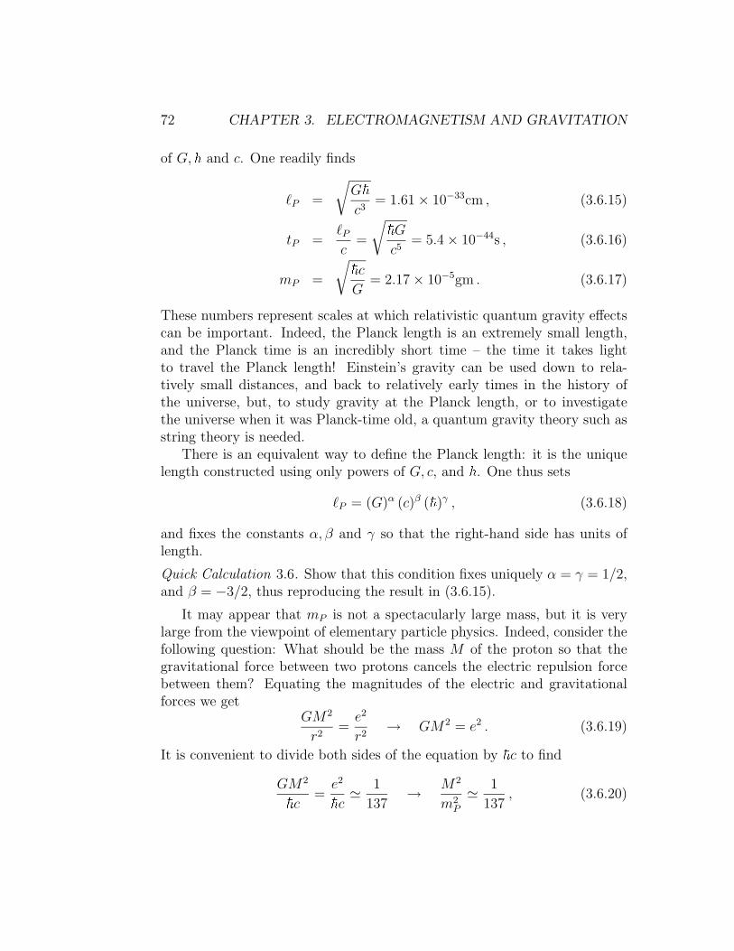
These numbers represent scales at which relativistic quantum gravity effectscan be important. Indeed, the Planck length is an extremely small length,and the Planck time is an incredibly short time – the time it takes lightto travel the Planck length! Einstein’s gravity can be used down to rela-tively small distances, and back to relatively early times in the history ofthe universe, but, to study gravity at the Planck length, or to investigatethe universe when it was Planck-time old, a quantum gravity theory such asstring theory is needed.

There is an equivalent way to define the Planck length: it is the uniquelength constructed using only powers of G, c, and �. One thus sets

�P = (G)α (c)β (�)γ , (3.6.18)

and fixes the constants α, β and γ so that the right-hand side has units oflength.

Quick Calculation 3.6. Show that this condition fixes uniquely α = γ = 1/2,and β = −3/2, thus reproducing the result in (3.6.15).

It may appear that mP is not a spectacularly large mass, but it is verylarge from the viewpoint of elementary particle physics. Indeed, consider thefollowing question: What should be the mass M of the proton so that thegravitational force between two protons cancels the electric repulsion forcebetween them? Equating the magnitudes of the electric and gravitationalforces we get

GM2

r2=

e2

r2→ GM2 = e2 . (3.6.19)

It is convenient to divide both sides of the equation by �c to find

GM2

�c=

e2

�c� 1

137→ M2

m2P

� 1

137, (3.6.20)

3.7. GRAVITATIONAL POTENTIALS 73

where use was made of (3.6.17). We thus find M � mP /12, or about one-tenth of the Planck mass. This is indeed a very large mass, about 1018 timesthe true mass of the proton.

3.7 Gravitational potentials

We want to learn what happens with the gravitational constants when wechange the dimensionality of spacetime. To find out, we can use Newtoniangravity, and work with gravitational potentials. Our immediate aim is tofind the equation relating the gravitational potential to the mass density inarbitrary number of dimensions. In the following section, this result will beused to define the Planck length in any number of dimensions.

We define a gravity field �g with units of force per unit mass, just as theelectric field has units of force per unit charge. The force on a given testmass m at a point where the gravity field is �g is given by m�g. We set this �gequal to minus the gradient of the gravitational potential Vg:

�g = −∇Vg . (3.7.1)

We will take this equation to be true in all dimensions. Equation (3.7.1) hascontent: if you move a particle along a closed loop in a static gravitationalfield, the net work you do against the gravitational field is zero.

Quick Calculation 3.7. Prove the above statement.

What are the units for the gravitational potential? Equation (3.7.1) gives

[Force]

M=

[Vg]

L⇒ [Vg] =

Energy

M. (3.7.2)

The gravitational potential has units of energy per unit mass in any dimen-sion. The gravitational potential V

(4)g of a point mass in four dimensions is

V (4)g = −GM

r. (3.7.3)

We can use the electromagnetic analogy to find the equation satisfied bythe gravitational potential. In electromagnetism, we found an equation forthe electric potential which holds in any dimension. It was given in (3.5.15):

∇2Φ = −4πρ . (3.7.4)


The four-dimensional scalar potential for a point charge is

Φ(4) =Q

r, (3.7.5)

and satisfies (3.7.4). It follows by analogy that the four-dimensional gravi-tational potential in (3.7.3) satisfies

∇2 V (4)g = 4πG ρm , (3.7.6)

where ρm is the matter density. While this equation is correct in four di-mensions, a small modification is needed for other dimensions. Note that theleft-hand side has the same units in any number of dimensions: the units of Vg

are always the same, and the laplacian always divides by length squared. Theright-hand side must also have the same units in any number of dimensions.Since ρm is a mass density, it has different units in different dimensions, andas a consequence the units of G must change when the dimensions change.We therefore rewrite the above equation more precisely as

∇2V (n)g = 4πG(n)ρm , (3.7.7)

when working in n-dimensional spacetime. In particular, we identify G(4) asthe four-dimensional Newton constant G. Equation (3.7.7) defines Newto-nian gravitation in arbitrary number of dimensions.

3.8 The Planck length in various dimensions

We can define the Planck length in any dimension just as we did in fourdimensions: the Planck length is the length built using only powers of thegravitational constant G(n), c and �. To compute the Planck length we mustdetermine the units of G(n). Let us therefore look at (3.7.7) and recall that theunits of the right-hand side must be the same in all dimensions. Comparingthe cases of five and four dimensions, for example,

[G(5)]M

L4= [G]

M

L3→ [G(5)] = L[G] . (3.8.1)

The units of G(5) have one more factor of length than those of G. Now wecan calculate the Planck length in five dimensions. First, we use (3.6.15) toread the units of G in terms of units of length and units of c and �:

[G] =[c]3 L2

[�]. (3.8.2)

3.9. GRAVITATIONAL CONSTANTS AND COMPACTIFICATION 75

Using (3.8.1), we get

[G(5)] =[c]3 L3

[�]. (3.8.3)

Since the Planck length is constructed uniquely from the gravitational con-stant, c, and �, we can remove the brackets in the above equation and replaceL by the five-dimensional Planck length:

(�(5)P )3 =

�G(5)

c3. (3.8.4)

Reintroducing the four-dimensional Planck length:

(�(5)P )3 =

(�G

c3

)G(5)

G→ (�

(5)P )3 = (�P )2G(5)

G. (3.8.5)

Since they do not have the same units, it does not make sense to compare di-rectly the gravitational constants in four and five dimensions. Planck lengths,however, can be compared. If the Planck length in four and five dimensionsare the same, G(5)/G = �P . In this case the gravitational constants differ byone factor of the common Planck length.

It is not hard to generalize the above equations to n spacetime dimensions:

Quick Calculation 3.8. Show that (3.8.4) and (3.8.5) are replaced by

(�(n)P

)n−2

=�G(n)

c3= (�P )2G(n)

G. (3.8.6)

3.9 Gravitational constants and compactifi-

cation

If string theory is correct, our world is really higher dimensional. The funda-mental gravity theory is defined in this higher-dimensional world, with somevalue for the higher-dimensional Planck length. Since we observe only fourdimensions, the additional dimensions may be curled up to form a compactspace with small volume. We can then ask: what is the effective value of thefour-dimensional Planck length? As we shall show here, the effective four-dimensional Planck length depends on the volume of the extra dimensions,as well as on the value of the higher-dimensional Planck length.


These observations raise the possibility that the Planck length in the effec-tively four-dimensional world – the famous number equal to about 10−33cm –may not coincide with the fundamental Planck length in the original higher-dimensional theory. Is it possible that the fundamental Planck length ismuch bigger than the familiar, four-dimensional one? We will answer thisquestion in the following section. Here we will now work out the effect ofcompactification on gravitational constants.

How do we calculate the gravitational constant in four dimensions if weare given the gravitational constant in five? First, we recognize the needto curl up one spatial dimension, otherwise there is no effectively four-dimensional spacetime. As we will see, the size of the extra dimension willenter into the relationship between the gravitational constants. To explorethese questions precisely, consider a five-dimensional spacetime where onedimension forms a small circle of radius R. We are given G(5) and would liketo calculate G(4).

Figure 3.2: A world with four space dimensions, one of which, x4, is compactifiedinto a circle of radius R. A ring of total mass M wraps around this compactdimension.

Let (x1, x2, x3) denote three spatial dimensions of infinite extent, and x4

denote a compactified dimension of circumference 2πR (see Figure 3.2). Weplace a uniform ring of total mass M all around the circle at x1 = x2 =x3 = 0. This is a constant mass distribution along the x4 dimension. Weare interested in the gravitational potential that emerges from such a massdistribution. We could have alternatively placed a point mass at some fixedx4, but this makes the calculations more involved (see Problem 3.8). In the

3.9. GRAVITATIONAL CONSTANTS AND COMPACTIFICATION 77

present case the gravitational potential cannot depend on x4. The total massM can be written as

Total Mass = M = 2πRm , (3.9.1)

where m is the mass per unit length.

What is the mass density in the five-dimensional world? It is only nonzeroat x1 = x2 = x3 = 0. To represent such mass density we must use deltafunctions. Recall that the delta function δ(x) can be viewed as a singularfunction whose value is zero except for x = 0 and such that the integral∫ ∞−∞ dxδ(x) = 1. This integral implies that if x has units of length, then

δ(x) has units of inverse length. Since the five-dimensional mass density isconcentrated at x1 = x2 = x3 = 0, it is reasonable to include in its formulathe product δ(x1)δ(x2)δ(x3) of three delta functions. We claim that

ρ(5) = mδ(x1)δ(x2)δ(x3) . (3.9.2)

We first check the units. The mass density ρ(5) must have units of M/L4.This works out since m has units of mass per unit length, and the three deltafunctions supply an additional factor of L−3. The ansatz in (3.9.2) could stillbe off by a constant dimensionless factor, a factor of two, for example. As afinal check, we integrate ρ(5) all over space. The result should be the totalmass:

∫ ∞

−∞dx1dx2dx3

∫ 2πR

0

dx4ρ(5)

= m

∫ ∞

−∞dx1δ(x1)

∫ ∞

−∞dx2δ(x2)

∫ ∞

−∞dx3δ(x3)

∫ 2πR

0

dx4

= m 2πR . (3.9.3)

This is indeed the total mass on account of (3.9.1). To the effectively four-dimensional observer, the correct expression for the mass density would be

ρ(4) = Mδ(x1)δ(x2)δ(x3) . (3.9.4)

For this observer, the mass is point-like and it is located at x1 = x2 = x3 = 0.Note the relation

ρ(5) =1

2πRρ(4) . (3.9.5)


Let us now use this information in the equations for the gravitationalpotential. In five-dimensional spacetime equation (3.7.7) gives

∇2(5)V

(5)g (x1, x2, x3, x4) = 4πG(5)ρ(5) =

4πG(5)

2πRρ(4) , (3.9.6)

where we also used (3.9.5). Since the mass distribution is x4-independent,

the potential V(5)g is also x4-independent, and the laplacian becomes the four-

dimensional one. We then get

∇2(4)V

(5)g (x1, x2, x3) = 4π

G(5)

2πRρ(4) . (3.9.7)

The effective four-dimensional gravitational potential is the five-dimensionalone, and the above equation has taken the form of the gravitational equationin four dimensions, where the constant in-between the 4π and the ρ(4) is thefour-dimensional gravitational constant. We have therefore shown that

G =G(5)

2πR→ G(5)

G= 2πR ≡ �C , (3.9.8)

where �C is the length of the extra compact dimension. This is what we wereseeking: a relationship between the strength of the gravitational constantsin different dimensions in terms of the size of the extra dimensions.

The generalization of (3.9.8) to the case where there is more than oneextra dimension is straightforward. One finds that

G(n)

G= (�C)n−4 , (3.9.9)

where �C is the common length of each of the extra dimensions. When thevarious dimensions are curled up into circles of different lengths, the aboveright-hand side must be replaced by the product of the various lengths. Thisproduct is, in fact, the volume of the extra dimensions.

3.10 Large extra dimensions

We are now done with all the groundwork. In section 3.8 we found the relationbetween the Planck length and the gravitational constant in any dimension.

3.10. LARGE EXTRA DIMENSIONS 79

In section 3.9 we determined how gravitational constants are related uponcompactification. We are ready to find out how the fundamental Plancklength in a higher dimensional theory with compactification is related to thePlanck length in the effectively four-dimensional theory.

Consider therefore a five-dimensional world, with Planck length �(5)P and

a single spatial coordinate curled up into a circle of circumference �C . Whatis then �P ? From (3.8.5) and (3.9.8) we find that

(�(5)P )3 = (�P )2 G(5)

G= (�P )2 �C . (3.10.1)

Solving for �P , we get

�P = �(5)P

√�(5)P

�C

. (3.10.2)

This relation enables us to explore the possibility that the world is actuallyfive-dimensional with a fundamental Planck length �

(5)P that is much larger

than 10−33 cm. Of course, we must have �P ∼ 10−33 cm. This is, after all thefour-dimensional Planck length, whose value is given in (3.6.15). What would

�C have to be for us to have an experimentally accessible �(5)P ∼ 10−18 cm?

Substituting �(5)P ∼ 10−18 cm and �P ∼ 10−33 cm into equation (3.10.2), we

find �C ∼ 1012 cm ∼ 107 km. This is a more than twenty times the distancefrom the earth to the moon. Such a large extra dimension would have beendetected long ago.

Having failed in five dimensions, let us try six space-time dimensions.Generally, equation (3.8.6), together with (3.9.9) gives

(�(n)P

)n−2

= (�P )2G(n)

G= (�P )2(�C)n−4 . (3.10.3)

After rearranging terms, we find that

�P = �(n)P

(�(n)P

�C

)n2−2

. (3.10.4)

Let’s assume that �(6)P ∼ 10−18 cm. With n = 6, equation (3.10.4) gives

10−33 ∼ 10−18(�

(6)P

�C

), (3.10.5)


which yields�C ∼ 10−3cm . (3.10.6)

This is a lot more interesting! Could there be extra dimensions 10−3 cmlong? You might think that this is still too big, since even microscopes probemuch smaller distances. In fact, accelerators probe distances of the orderof 10−18cm. Surprisingly, it is possible that these “large extra dimensions”exist, and that we have not observed them yet.

How would we confirm the existance of additional dimensions? By test-ing the force law giving the gravitational attraction between two masses.For distances much larger than the compactification scale �C the world iseffectively four-dimensional, and the force between two masses must followaccurately Newton’s law of inverse squared dependence on the separation. Onthe other hand, for distances smaller than �C , the world is effectively higher-dimensional, and the force law must change. If we detect that for smalldistances the force between masses goes like r−4, where r is the separation,then this is consistent with the existance of two compact extra dimensions.Tests of gravity at small distances are very difficult to do. Gravity has notbeen tested accurately enough below a millimeter. So there is very littleevidence that at short distance scales, gravity obeys an inverse squared law.

You might ask: what about forces other than gravity? Electromagnetismhas been tested to much smaller distances, and we do know that the electricforce obeys an inverse squared law very accurately. This seems to rule outlarge extra dimensions. The possibility of large extra dimensions, however,exists in string theory, where our spatial world could be a three-dimensionalhyperplane transverse to the extra dimension. This hyperplane is called aD3-brane, a D-brane with three spatial dimensions.

Open strings have the remarkable property that their endpoints are stuckto the D-branes. In many phenomenological models of string theory thefluctuations of open strings give rise to the familiar leptons, quarks, andgauge fields, including the Maxwell gauge field. It follows that these fields arebound to the D3-brane and do not feel the extra dimensions. Closed stringsare not bound by D3-branes, and therefore gravity, which arises from closedstrings, is affected by the extra dimensions. The appropriate gravitationalexperiments, however, do not yet rule out extra dimensions if they are smallerthan a tenth of a millimeter.

Even though the Planck length �P is an important length scale in fourdimensions, if there are large extra dimensions, the truly fundamental Planck

3.10. LARGE EXTRA DIMENSIONS 81

length would be much bigger than the effective four-dimensional one. Thepossibility of large extra dimensions is slightly unnatural – why should theextra dimensions be much larger than the fundamental length scale? Themost natural possibility is that the extra dimensions have the size of thefundamental length scale, in which case the fundamental length scale remainsthe fundamental one in lower dimensions (see (3.10.4)). Thus many physicistsbelieve it is unlikely that there are large extra dimensions. What is trulystriking is that even if they are there, we would have not detected themyet. Physicists are currently doing experiments to find out if large extradimensions exist.


Problems

Problem 3.1. Lorentz covariance for motion in EM fields

The Lorentz force equation (3.1.5) can be written relativistically as

dpµ

ds= qF µνuν , (1)

where uν is the four-velocity, and pµ is the four-momentum. Check explicitlythat this equation reproduces (3.1.5) when µ is a spatial index. What does(1) give when µ = 0? Does it make sense? Is equation (1) gauge invariant?

Problem 3.2. Maxwell equations in four dimensions

(a) Show explicitly that the two source-free Maxwell equations emerge fromthe conditions Tµλν = 0.

(b) Show explicitly that the two Maxwell equations with sources emergefrom (3.3.23).

Problem 3.3. E&M in three dimensions

(a) Begin with Maxwell’s equations and the force law in four dimensions,and find the reduced equations in three dimensions by using the ansatz(3.2.1) and assuming that no field can depend on the z-direction.

(b) Repeat the analysis of three-dimensional electromagnetism by startingwith the Lorentz covariant formulation. Take Aµ = (Φ, A1, A2), andexamine Fµν , the Maxwell equations (3.3.23) and the relativistic formof the force law derived in Problem 3.1.

Problem 3.4. Electric fields and potentials of point charges.

(a) Show that for time-independent fields, the Maxwell equation T0ij = 0implies that ∂iEj − ∂jEi = 0. Explain why this condition is satisfied

by the ansatz �E = −∇Φ.

(b) Show that with n spatial dimensions, the potential Φ due to a pointcharge Q is given by

Φ(r) =Γ(

n2− 1

)π

n2−1

Q

rn−2.

Problems for Chapter 3 83

Problem 3.5. Analytic continuation for gamma functions.

Consider the definition of the gamma function for complex arguments zwhose real part is positive:

Γ(z) =

∫ ∞

0

dt e−ttz−1 , �(z) > 0 . (1)

Use the above equation to show that for �(z) > 0

Γ(z) =

∫ 1

0

dt tz−1(e−t −

N∑n=0

(−t)n

n!

)+

N∑n=0

(−1)n

n!

1

z + n+

∫ ∞

1

dt e−ttz−1 .

Explain why the above right-hand side is well-defined for �(z) > −n − 1. Itfollows that this right-hand side provides the analytic continuation of Γ(z) for�(z) > −n−1. Conclude that the gamma function has poles at 0,−1,−2, . . .,and give the value of the residue at z = −n (with n a positive integer).

Problem 3.6. Planetary motion in four and higher dimensions.

Consider the motion of planets in planar orbits around heavy stars in ourfour dimensional world and in worlds with additional spatial dimensions. Wewish to study the stability of these orbits under perturbations that keep themplanar. Such a perturbation would arise, for example, if a meteorite movingon the plane of the orbit hits the planet and changes its angular momentum.Show that while planetary orbits in our four dimensional world are stable

under such perturbations, they are not so in five or higher dimensions, whereupon meteorite impact the planet would either spiral in towards the star,or spiral out to infinity. [Hint: You may find it useful to use the effectivepotential for motion in a central force field.].

Problem 3.7. Gravitational field of a point mass in compactified five dimen-sional world.

Consider five dimensional space-time with space coordinates (x, y, z, w)not yet compactified and consider a point mass of mass M located at theorigin (x, y, z, w) = (0, 0, 0, 0).

(a) Find the gravitational potential V(5)g (r) due to this point mass. Here

r = (x2 + y2 + z2 + w2)1/2, and your answer should be in terms of G(5).

You may use the equation ∇2V(5)g = 4πG(5)ρM , and the divergence

theorem.


Figure 3.3: Problem 3.8: Point mass M in a five spacetime dimensional worldwith one extra compact dimension.

Now let w become a circle with radius a keeping the same mass at thesame point, as shown in Figure 3.3.

(b) Write an exact expression for the gravitational potential V(5)g (x, y, z, 0).

This potential is in fact a function of R ≡ (x2 + y2 + z2)1/2, and can bewritten as an infinite sum.

(c) Show that for R >> a the above gravitational potential takes the formof a four-dimensional gravitational potential, with Newton’s constantG(4) given in terms of G(5) as calculated in class. [Hint: turn the infinitesum into an integral].

These results, confirm both the relation between the four and five di-mensional Newton constants for a compactification, and the emergence of afour-dimensional potential at distances large compared to the compactifica-tion size.

Problem 3.8. Exact answer for gravitational potential.

The infinite sum in Problem 3.8 can be evaluated exactly using the iden-tity

∞∑n=−∞

1

1 + (πnx)2=

1

xcoth

(1

x

).

Problems for Chapter 3 85

(a) Find an exact expression for the gravitational potential in the com-pactified theory.

(b) Expand this answer to calculate the leading correction to the gravita-tional potential in the limit when a < R. For what value of R/a is thecorrection of order 1%?

(c) Use the exact answer in (a) to calculate also the potential when R < a,giving the first two terms in the expansion. Do you recognize theleading term?

Documents

Chapter 3 Electromagnetism and Gravitation in Various ...fma.if.usp.br/~amsilva/Livros/Zwiebach/chapter3.pdf · Chapter 3 Electromagnetism and Gravitation in Various Dimensions String