Embed Size (px)
Citation preview

Chapter 3
Despair Inc.
POLYMERIZATION KINETICS REVIEW
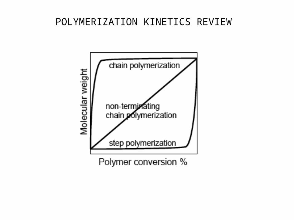
[Reproduced from G. M. Kavanagh and S. B. Ross-Murphy, “Rheological characterisation of polymer gels”, Prog. Polym. Sci. 23, 533 (1998).]
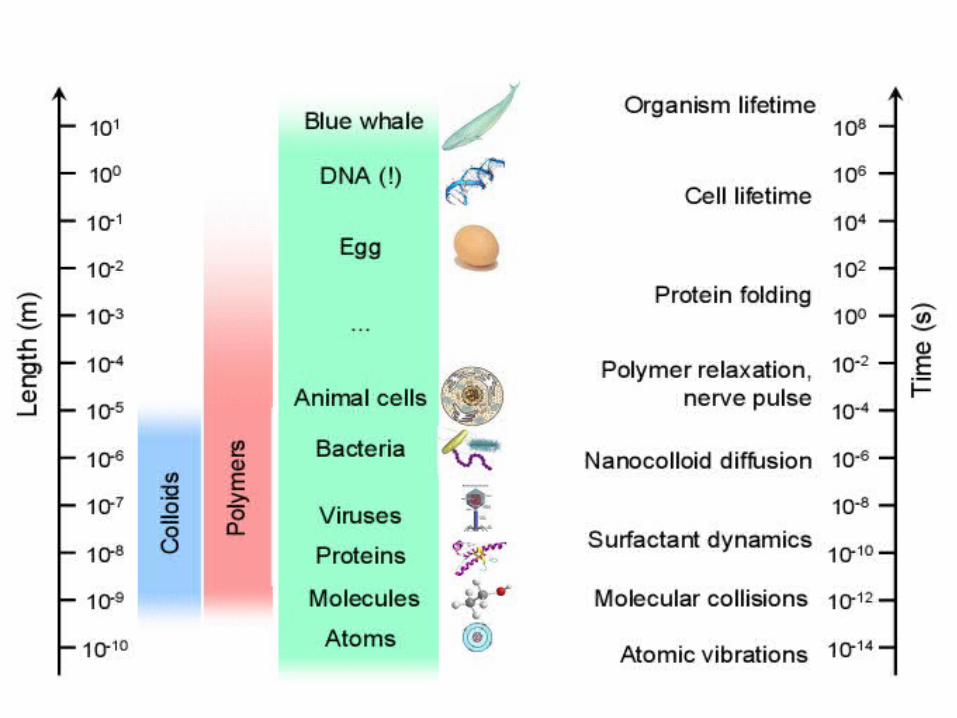
Characterization of polymers: Length and time scales are important
Polymer solubility
• In solvent, other polymer(s) or plasticizer• Non-Newtonian properties: Viscosity, rheology• Need to understand the configuration,
conformation, and dynamics of macromolecules– Statistical mechanics
• Series of mathematical models• Tied to experiment (viscosity, light scattering)
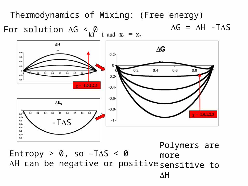
Thermodynamics of Mixing: (Free energy)
Entropy > 0, so –TS < 0H can be negative or positive
G = H -TS
-TS
For solution G < 0
Polymers are more sensitive to H

Spinoidal decomposition of a solution into two phases
• Quenching (rapid cooling) of solution• Polymer rich & polymer poor phases
Careful removal of polymer poor phase “microporous”Foams.
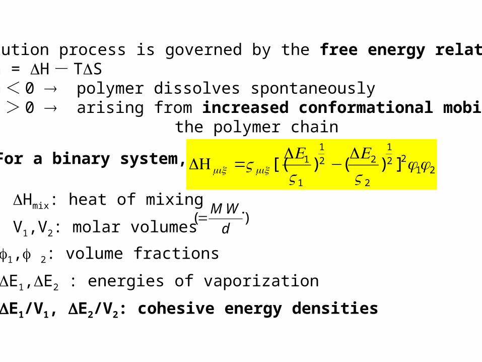
Any solution process is governed by the free energy relationship G = H - TS G < 0 polymer dissolves spontaneously S > 0 arising from increased conformational mobility of the polymer chain
For a binary system,21
22
1
2
22
1
1
1 ])()[( φφVE
VE
Vmixmix
−
=Η
)..
(d
WM=
Hmix: heat of mixing
V1,V2: molar volumes
1, 2: volume fractions
E1,E2 : energies of vaporization
E1/V1, E2/V2: cohesive energy densities
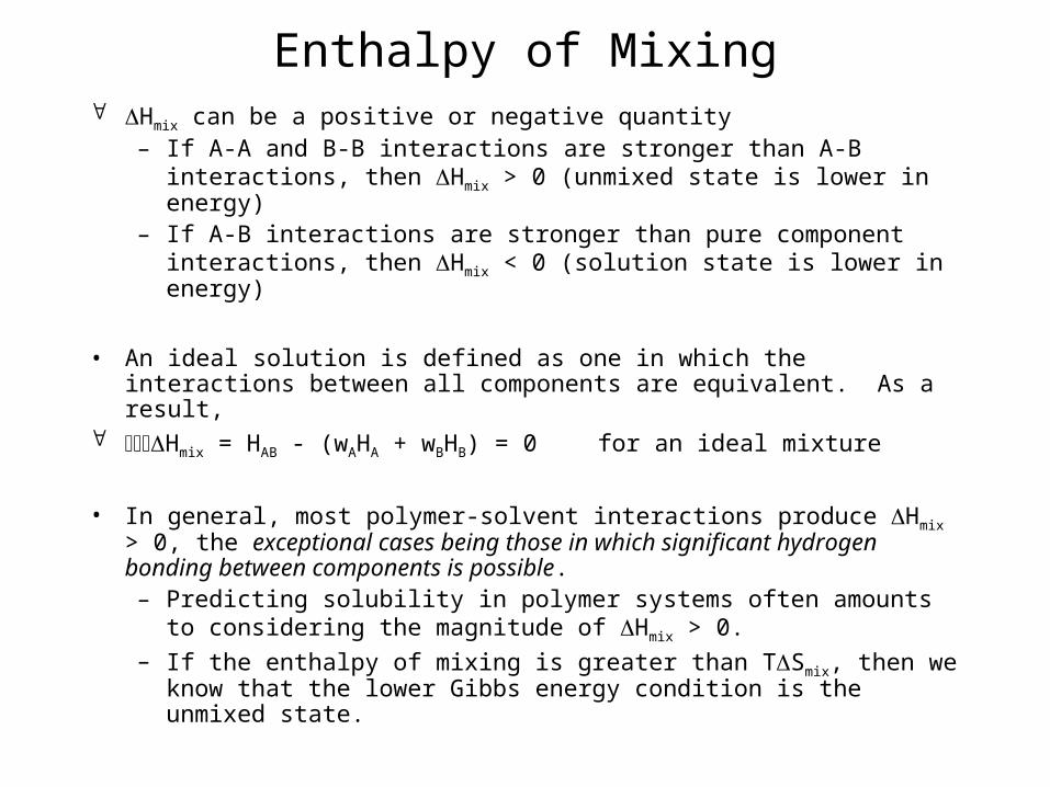
Enthalpy of Mixing Hmix can be a positive or negative quantity
– If A-A and B-B interactions are stronger than A-B interactions, then Hmix > 0 (unmixed state is lower in energy)
– If A-B interactions are stronger than pure component interactions, then Hmix < 0 (solution state is lower in energy)
• An ideal solution is defined as one in which the interactions between all components are equivalent. As a result,
Hmix = HAB - (wAHA + wBHB) = 0 for an ideal mixture
• In general, most polymer-solvent interactions produce Hmix > 0, the exceptional cases being those in which significant hydrogen bonding between components is possible.– Predicting solubility in polymer systems often amounts to
considering the magnitude of Hmix > 0.– If the enthalpy of mixing is greater than TSmix, then we know that
the lower Gibbs energy condition is the unmixed state.
2
1
1
11 )(
V
E=δ 2
1
2
22 )(
V
E=δ
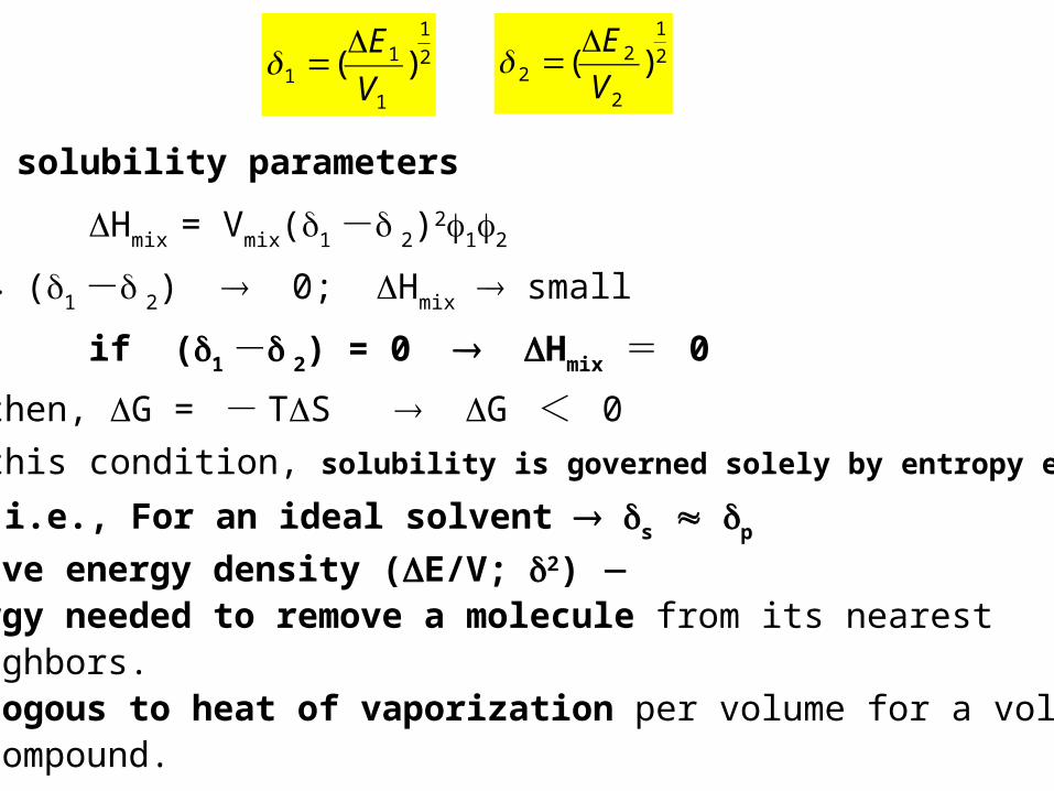
δ1, δ2: solubility parameters
Hmix = Vmix(δ1 -δ 2)212
∴ (δ1 -δ 2) 0; Hmix small
if (δ1 -δ 2) = 0 Hmix = 0
then, G = - TS G < 0
Under this condition, solubility is governed solely by entropy effects
i.e., For an ideal solvent δs δp
Cohesive energy density (E/V; δ2) ● energy needed to remove a molecule from its nearest neighbors.● analogous to heat of vaporization per volume for a volatile compound.
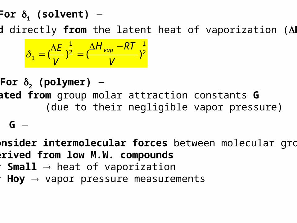
calculated directly from the latent heat of vaporization (Hvap)
For δ1 (solvent)
2
1
2
1
1 )()(V
RTH
V
E vap −=
=δ
For δ2 (polymer) estimated from group molar attraction constants G (due to their negligible vapor pressure)
G
● Consider intermolecular forces between molecular groups● Derived from low M.W. compounds● by Small heat of vaporization● by Hoy vapor pressure measurements
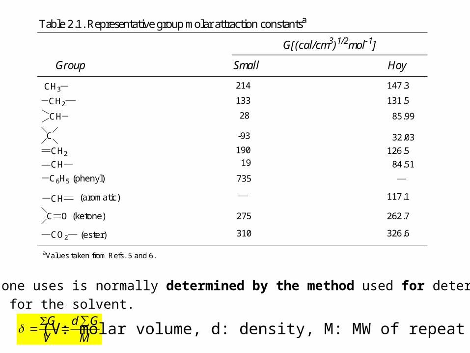
Table 2.1. Representative group molar attraction constantsa
Group
G[(cal/cm3)1/2mol-1]
Small Hoy
CH3
CH2
CH
C
CH2
CH
C6H5 (phenyl)
C O (ketone)
CO2 (ester)
214
133
28
-93
190
19
735
275
310
CH
147.3
131.5
85.99
32.03
126.5
84.51
117.1
262.7
326.6
aValues taken from Refs. 5 and 6.
(aromatic)
Which set one uses is normally determined by the method used for determining δ1
for the solvent.
M
Gd
V
G ∑=
Σ=δ (V: molar volume, d: density, M: MW of repeat unit)

CH2 CH
C6H5
Small’s system 0.9104
)73528133(05.1=
++=δ
Hoy’s system 3.9104
)]1.117(699.855.131[05.1=
++=δ
For taking into account the strong intermolecular dipolar forces,
solubility parameters δd (dispersion forces)δp (dipole-dipole attraction)δH (hydrogen bonding)
Hydrodynamic volume polymer size in solution●Interaction between solvent and polymer molecules●Chain branching●Conformational effects (arising from the polarity and steric bulkiness of the substituent groups)Restricted rotation caused by resonance
C NH
O
C NH
O
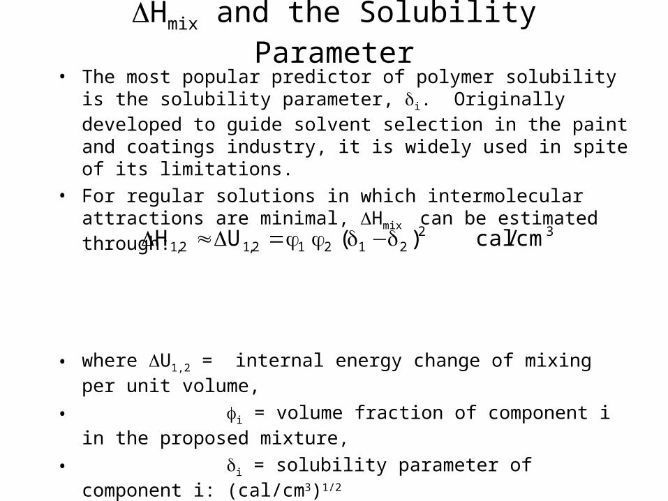
Hmix and the Solubility Parameter
• The most popular predictor of polymer solubility is the solubility parameter, δi. Originally developed to guide solvent selection in the paint and coatings industry, it is widely used in spite of its limitations.
• For regular solutions in which intermolecular attractions are minimal, Hmix can be estimated through:
• where U1,2 = internal energy change of mixing per unit volume,
• i = volume fraction of component i in the proposed mixture,
• δi = solubility parameter of component i: (cal/cm3)1/2
• Note that this formula always predicts Hmix > 0, which holds only for regular solutions.
3221212,12,1 cm/cal)(UH δ−δφφ=≈
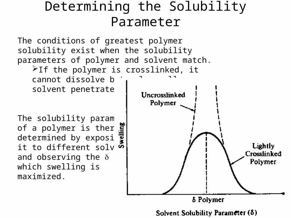
The conditions of greatest polymer solubility exist when the solubility parameters of polymer and solvent match.
If the polymer is crosslinked, it cannot dissolve but only swell as solvent penetrates the material.
The solubility parameter of a polymer is therefore determined by exposing it to different solvents, and observing the δ at which swelling is maximized.
Determining the Solubility Parameter
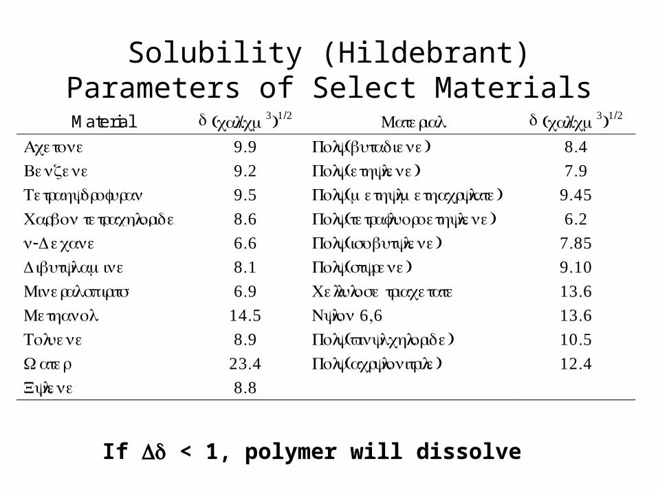
Solubility (Hildebrant) Parameters of Select Materials
Material δ (cal/cm3)1/2 Material δ (cal/cm3)1/2
Acetone 9.9 Poly(butadiene) 8.4Benzene 9.2 Poly(ethylene) 7.9Tetrahydrofuran 9.5 Poly(methylmethacrylate) 9.45Carbon tetrachloride 8.6 Poly(tetrafluoroethylene) 6.2n-Decane 6.6 Poly(isobutylene) 7.85Dibutyl amine 8.1 Poly(styrene) 9.10Mineral spirits 6.9 Cellulose triacetate 13.6Methanol 14.5 Nylon 6,6 13.6Toluene 8.9 Poly(vinyl chloride) 10.5Water 23.4 Poly(acrylonitrile) 12.4Xylene 8.8
If δ < 1, polymer will dissolve
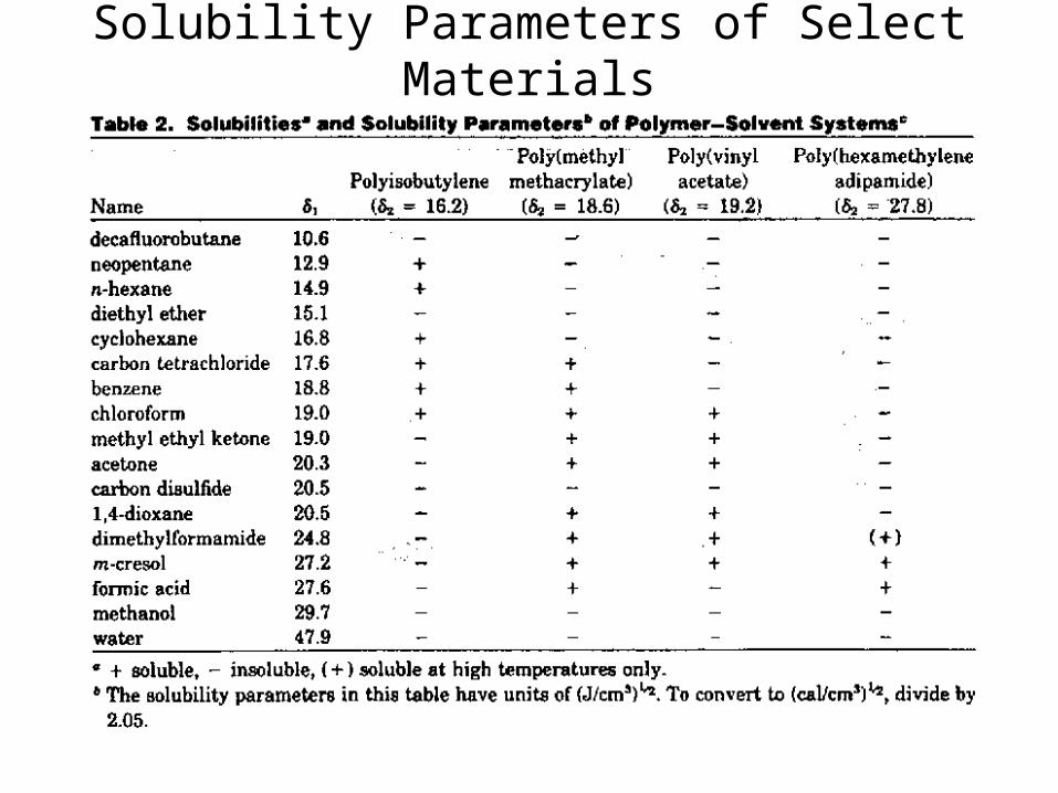
Solubility Parameters of Select Materials
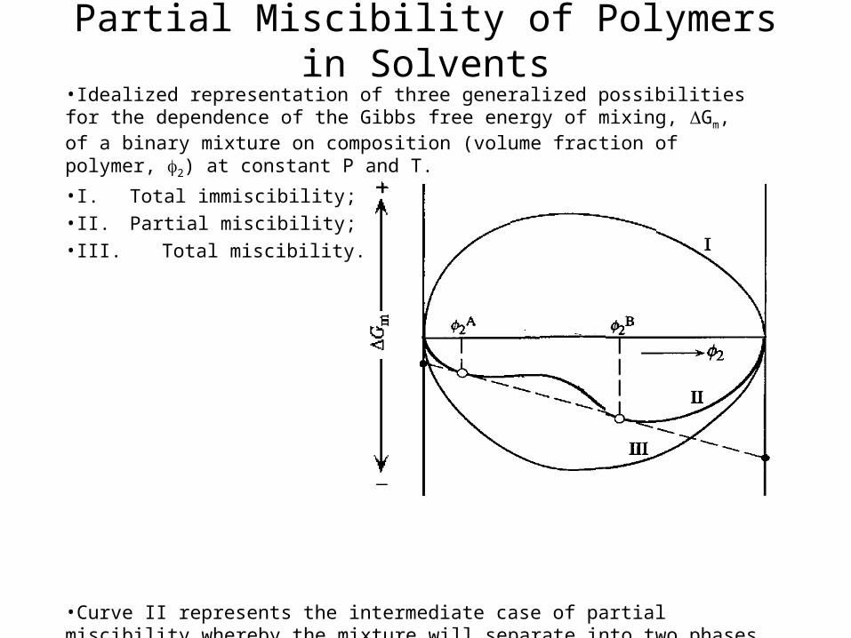
Partial Miscibility of Polymers in Solvents•Idealized representation of three generalized possibilities for the dependence of the Gibbs free energy of mixing, Gm, of a binary mixture on composition (volume fraction of polymer, 2) at constant P and T.
•I. Total immiscibility; •II. Partial miscibility; •III. Total miscibility.
•Curve II represents the intermediate case of partial miscibility whereby the mixture will separate into two phases whose compositions () are marked by the volume-fraction coordinates, 2
A and 2B, corresponding to points of common tangent to the
free-energy curve.

Factors Influencing Polymer-Solvent Miscibility
Based on the Flory-Huggins treatment of polymer solubility, we can explain the influence of the following variables on miscibility:
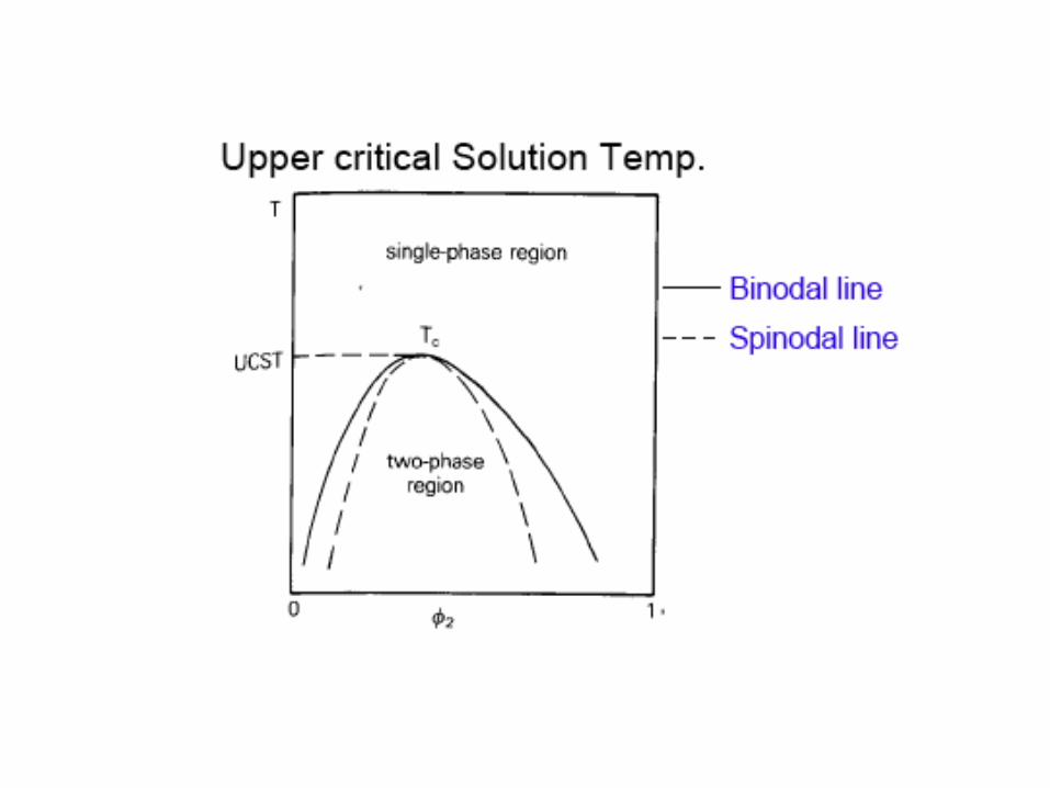
1. Temperature: The sign of Gmix is determined by the Flory- Huggins interaction parameter, .
As temperature rises, decreases thereby improving solubility.Upper solution critical temperature (UCST) behaviour is explained by Flory-Huggins theory, but LCST is not.
2. Molecular Weight: Increasing molecular weight reduces the configurational entropy of mixing, thereby
reducing solubility.
3. Crystallinity: A semi-crystalline polymer has a more positiveHmix = HAB - xAHA - xBHB due to the heat offusion that is lost upon mixing.

Theta Temperature

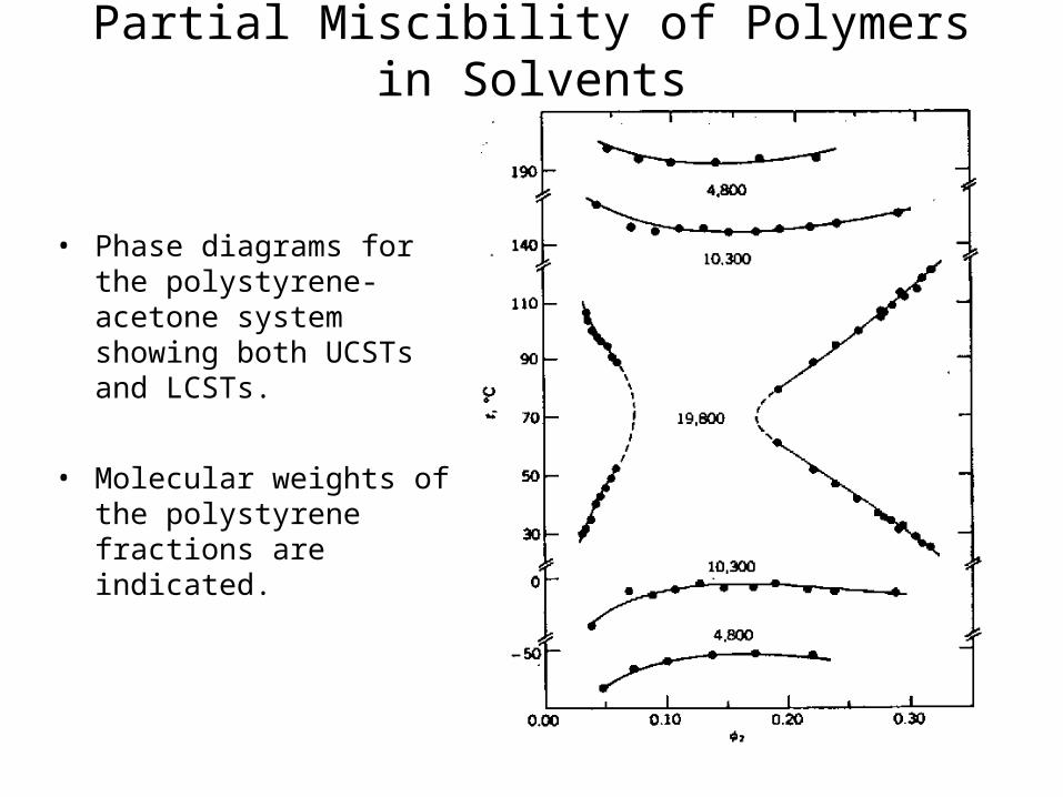
Partial Miscibility of Polymers in Solvents
• Phase diagrams for the polystyrene-acetone system showing both UCSTs and LCSTs.
• Molecular weights of the polystyrene fractions are indicated.
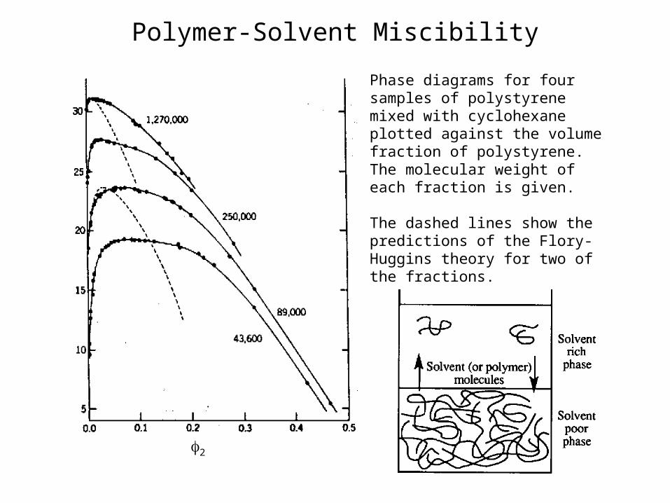
Polymer-Solvent Miscibility
2
Phase diagrams for four samples of polystyrene mixed with cyclohexane plotted against the volume fraction of polystyrene. The molecular weight of each fraction is given.
The dashed lines show the predictions of the Flory-Huggins theory for two of the fractions.
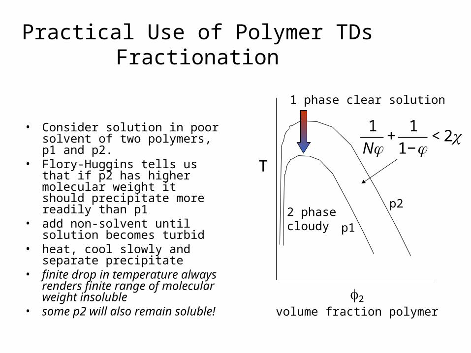
Practical Use of Polymer TDsFractionation
• Consider solution in poor solvent of two polymers, p1 and p2.
• Flory-Huggins tells us that if p2 has higher molecular weight it should precipitate more readily than p1
• add non-solvent until solution becomes turbid
• heat, cool slowly and separate precipitate
• finite drop in temperature always renders finite range of molecular weight insoluble
• some p2 will also remain soluble!
T
2
volume fraction polymer
p1
p22 phasecloudy
1 phase clear solution
φφ
21
11<
−+
N

Fractionation of Polymers using Precipitation

Industrial Relevance of Polymer Solubility
Polymer Solvent Effect ApplicationDiblockcopolymers
Motor Oil Colloidal suspensionsdissolve at high T,raising viscosity
Multiviscosity motoroil (10W40)
Poly(ethyleneoxide)
Water Reduces turbulent flow Heat exchangesystems, lowerspumping costs
Polyurethanes,cellulose esters
Esters, alcohols,various
Solvent vehicleevaporates, leaving filmfor glues
Varnishes, shellacand adhesives
Poly(vinyl chloride) Dibutylphthalate
Plasticizes polymer Lower polymer Tg,making “vinyl”
Polystyrene Poly(phenyleneoxide)
Mutual solution,toughens polystyrene
Impact resistantobjects, appliances
Polystyrene Triglyceride oils Phase separates uponoil polymerization
Oil-based paints,tough, hard coatings
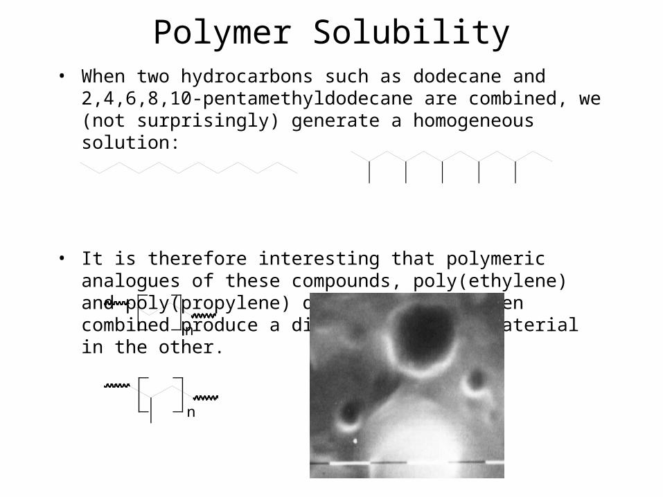
Polymer Solubility• When two hydrocarbons such as dodecane and 2,4,6,8,10-
pentamethyldodecane are combined, we (not surprisingly) generate a homogeneous solution:
• It is therefore interesting that polymeric analogues of these compounds, poly(ethylene) and poly(propylene) do not mix, but when combined produce a dispersion of one material in the other.
n
n

Polymer solutions: Definitions • Configuration: arrangement of atoms through bonds
– Inter-change requires bond breaking and making (>200 kJ/mol)– Different compositions of polymers– Different isomers or stereochemistries
• Conformation: within the constraints of a configuration, the possible arrangement(s) of atoms in space– Interchange requires bond rotations, but no bonds are broken or
made (can have non-bonding , ie. hydrogen bonding)
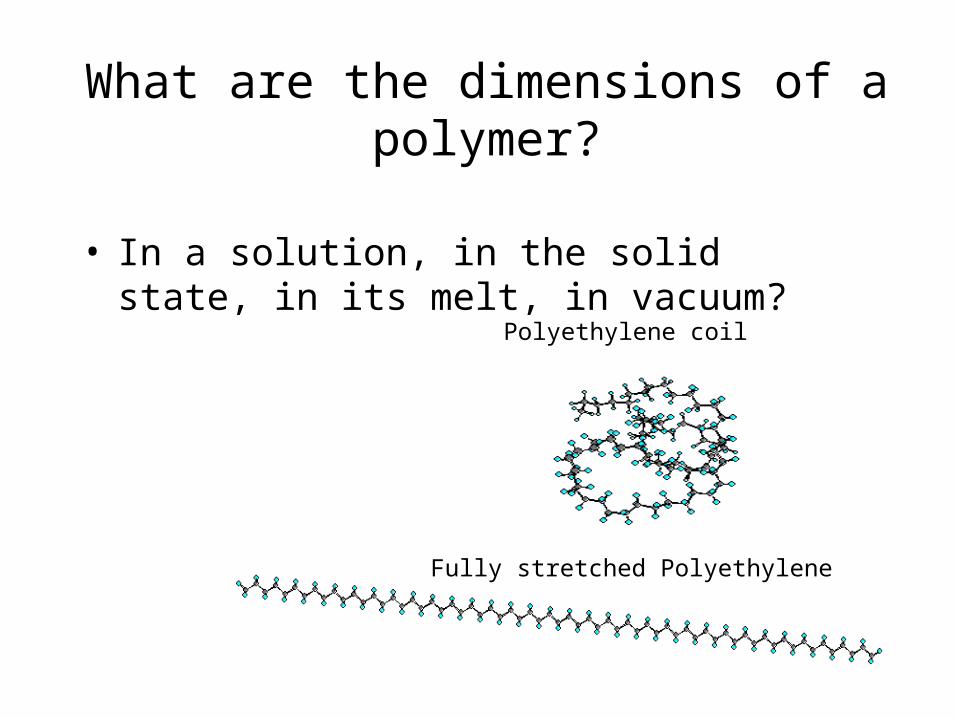
What are the dimensions of a polymer?
• In a solution, in the solid state, in its melt, in vacuum?
Fully stretched Polyethylene
Polyethylene coil
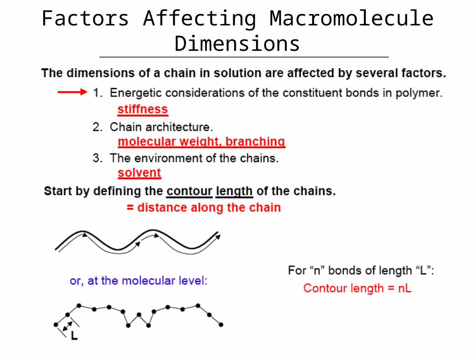
Factors Affecting Macromolecule Dimensions

Polymer Conformations
Flexible coil
Rigid rod
And everything in between
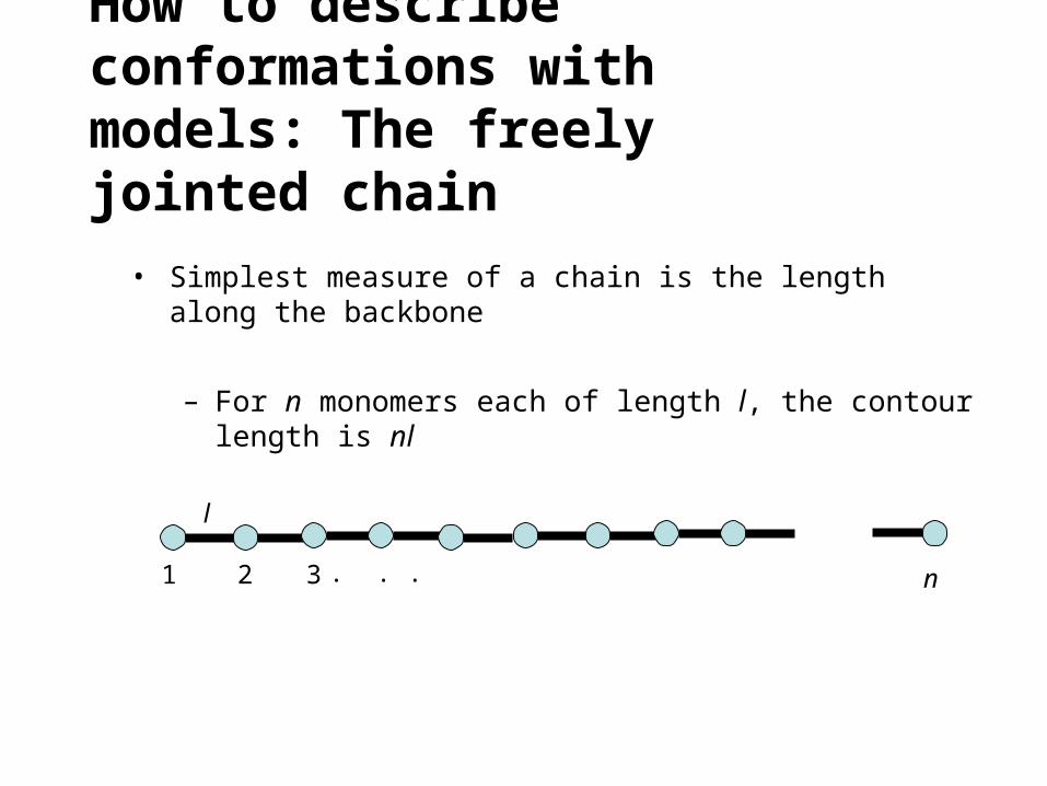
How to describe conformations with models: The freely jointed chain
• Simplest measure of a chain is the length along the backbone
– For n monomers each of length l, the contour length is nl
1 2 3 n. . .
l
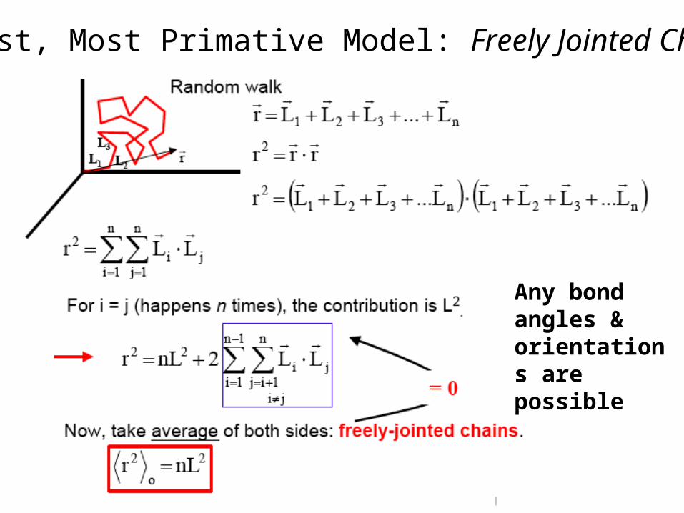
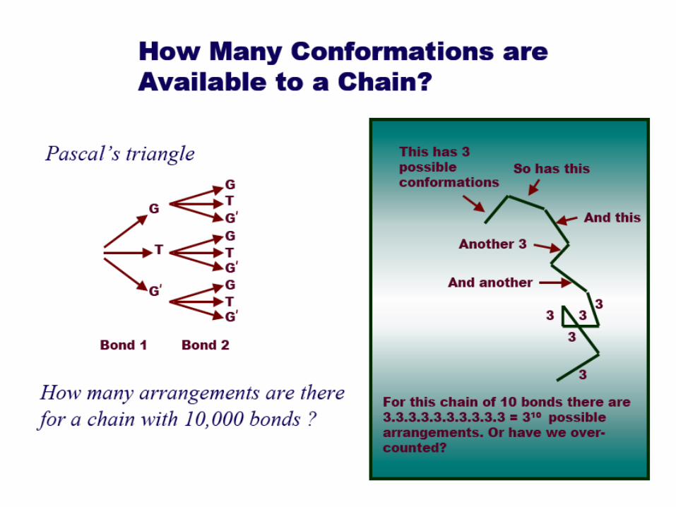
First, Most Primative Model: Freely Jointed Chain
Any bond angles & orientations are possible
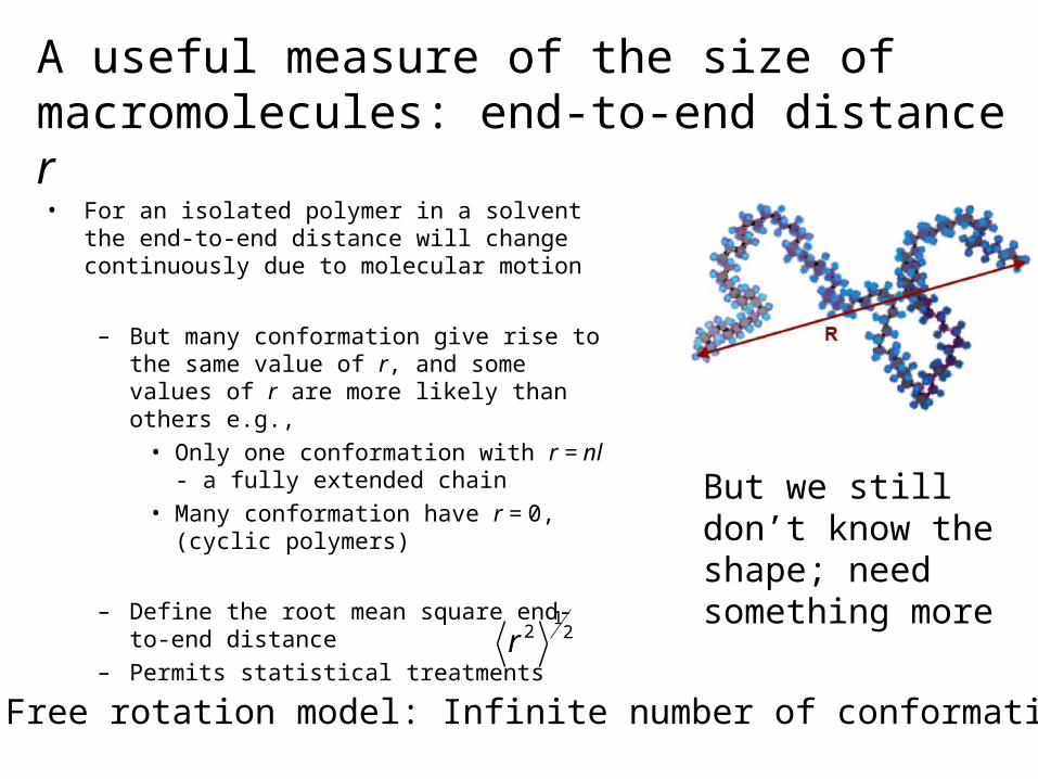
• For an isolated polymer in a solvent the end-to-end distance will change continuously due to molecular motion
– But many conformation give rise to the same value of r, and some values of r are more likely than others e.g.,
• Only one conformation with r = nl - a fully extended chain
• Many conformation have r = 0, (cyclic polymers)
– Define the root mean square end-to-end distance
– Permits statistical treatments1
2 2r
A useful measure of the size of macromolecules: end-to-end distance r
Free rotation model: Infinite number of conformations
But we still don’t know the shape; need something more
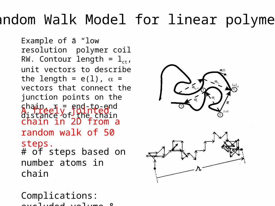
Example of a “low resolution” polymer coil RW. Contour length = lct, unit vectors to describe the length = e(l), = vectors that connect the junction points on the chain, r = end-to-end distance of the chain
A freely jointed chain in 2D from a random walk of 50 steps.
Random Walk Model for linear polymers
# of steps based on number atoms in chain
Complications: excluded volume & steric limitations
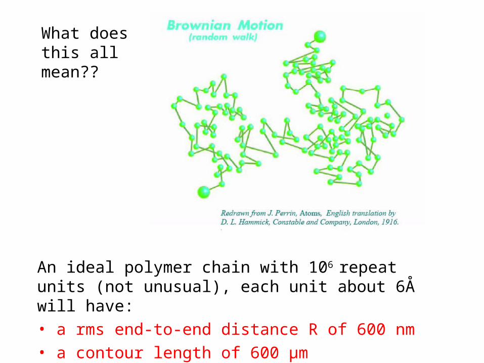
An ideal polymer chain with 106 repeat units (not unusual), each unit about 6Å will have:• a rms end-to-end distance R of 600 nm• a contour length of 600 μm
What does this all mean??
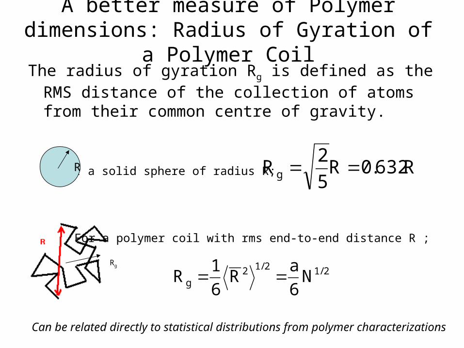
A better measure of Polymer dimensions: Radius of Gyration of a Polymer Coil
The radius of gyration Rg is defined as the RMS distance of the collection of atoms from their common centre of gravity.
For a solid sphere of radius R; R632.0R5
2R g ==
For a polymer coil with rms end-to-end distance R ;
2/12/12g N
6
aR
6
1R ==
R
Can be related directly to statistical distributions from polymer characterizations
Rg
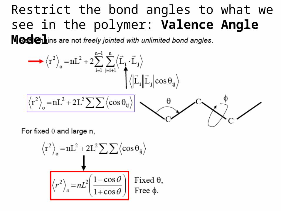
Restrict the bond angles to what we see in the polymer: Valence Angle Model

Valence angle model
• Simplest modification to the freely jointed chain model– Introduce bond angle restrictions
– Allow free rotation about bonds
– Neglecting steric effects (for now)
• If all bond angles are equal to ,
indicates that the result is for the valence angle model
• E.g. for polyethylene = 109.5° and cos ~ -1/3, hence,
2 2 (1 - cos )
(1 cos )far nl
< > =+
2 2 2far nl< > ≈

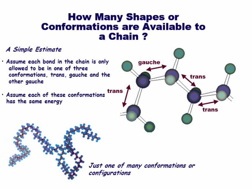
Finite Number of Conformations due to torsional & steric interactions: Restricted Rotation Angle
The energy barrier between gauche and trans is about 2.5 kJ/mol
RT~8.31*300 J/mol~2.5 kJ/mol


Equivalent Freely Jointed Chain Model
C∞ is a function of the stiffness of the chain. Higher is stiffer
C∞

• In general
– where is the steric parameter, which is usually determined for each polymer experimentally
– A measure of the stiffness of a chain is given by the characteristic ratio
– C typically ranges from 5 - 12
2 2 20
(1 - cos )
(1 cos )r nl
< > =+
2 20 / C r nl∞ = < >
Steric parameter and the characteristic ratio
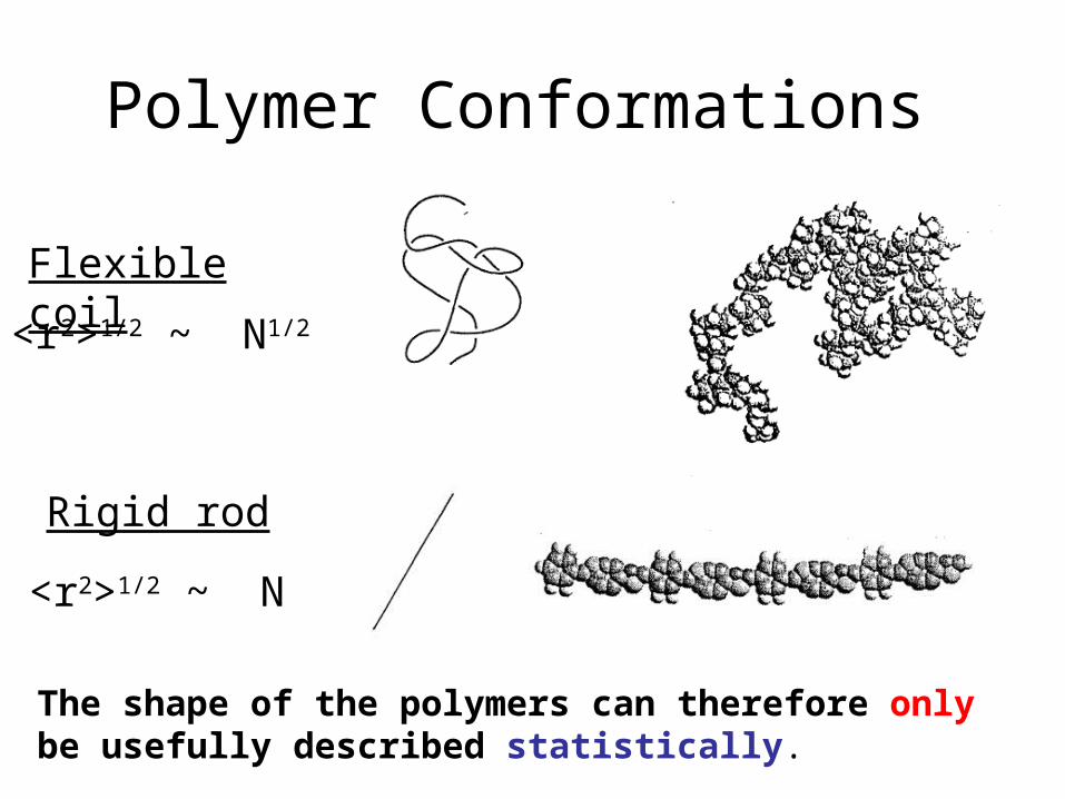
Polymer Conformations
Flexible coil
Rigid rod
<r2>1/2 ~ N1/2
<r2>1/2 ~ N
The shape of the polymers can therefore only be usefully described statistically.
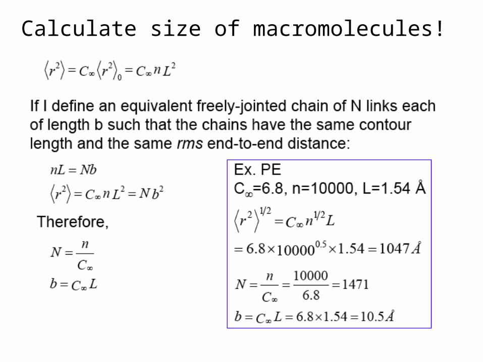
Calculate size of macromolecules!
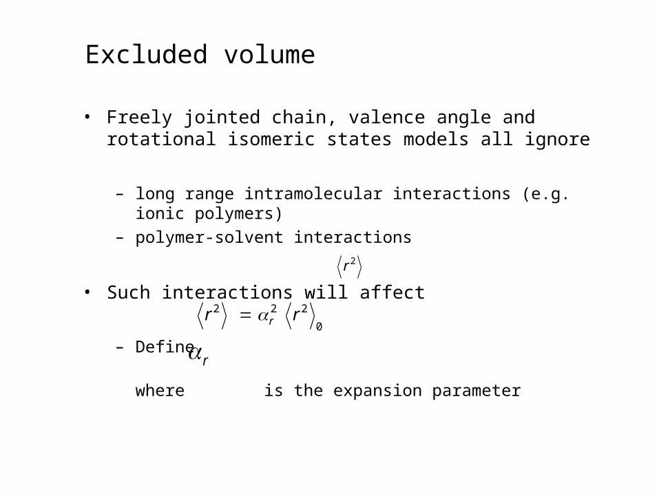
• Freely jointed chain, valence angle and rotational isomeric states models all ignore
– long range intramolecular interactions (e.g. ionic polymers)
– polymer-solvent interactions
• Such interactions will affect
– Define
where is the expansion parameter
Excluded volume
2 2 2
0 rr r=
2 r
r

Space filling?
The random walk and the steric limitations makes the polymer coils in a polymer melt or in a polymer glass “expanded”.
However, the overlap between molecules ensure space filling

Expansion Factors: Measure of solvent -Polymer Interactions
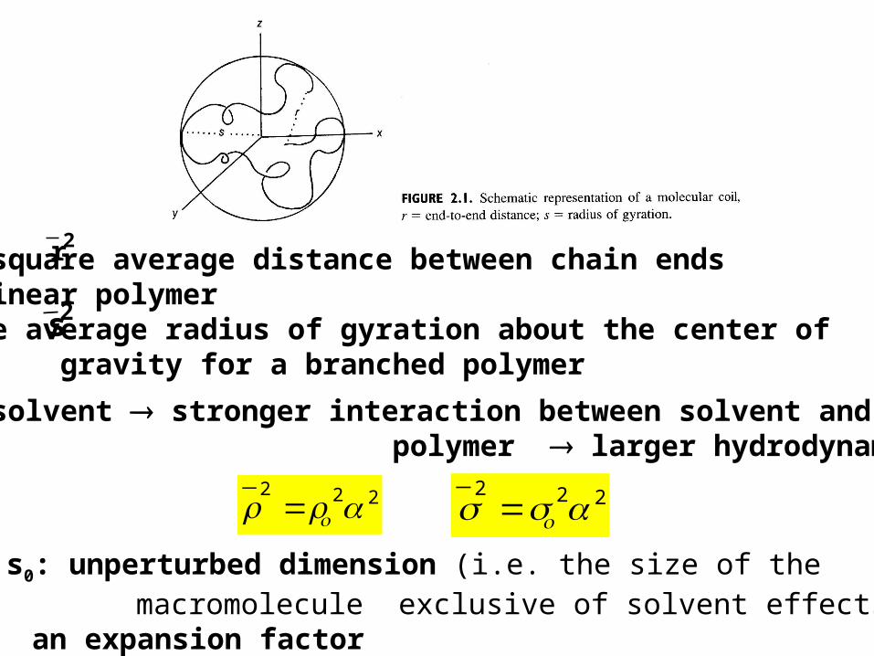
: mean-square average distance between chain ends for a linear polymer: square average radius of gyration about the center of gravity for a branched polymer
Better solvent stronger interaction between solvent and polymer larger hydrodynamic volume
r2
s2
222orr = 222
oss =
r0, s0: unperturbed dimension (i.e. the size of the macromolecule exclusive of solvent effects) : an expansion factor
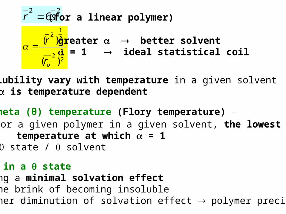
226sr = (for a linear polymer)
2
12
2
12
)(
)(
or
r= greater better solvent
= 1 ideal statistical coil
Solubility vary with temperature in a given solvent is temperature dependent
Theta (θ) temperature (Flory temperature) ● For a given polymer in a given solvent, the lowest temperature at which = 1● state / solvent
Polymer in a state• having a minimal solvation effect • on the brink of becoming insoluble• further diminution of solvation effect polymer precipitation

The expansion parameter r Solvent Effects on the Macromolecules
• r depends on balance between i) polymer-solvent and ii) polymer-polymer interactions
– If polymer-polymer are more favourable than polymer-solvent • r < 1• Chains contract• Solvent is poor
– If polymer-polymer are less favourable than polymer-solvent • r > 1• Chains expand• Solvent is good
– If these interactions are equivalent, we have theta condition• r = 1 • Same as in amorphous melt

The theta temperature• For most polymer solutions r depends on temperature, and increases
with increasing temperature
• At temperatures above some theta temperature, the solvent is good, whereas below the solvent is poor, i.e.,
What determines whether or not a polymer is soluble?
T > r > 1
T = r = 1
T < r < 1
Often polymers will precipitate out of solution, rather than contracting
Solubility of Polymers
Encyclopedia of Polymer Science, Vol 15, pg 401 says it best...A polymer is often soluble in a low molecular weight liquid if:
•the two components are similar chemically or are so constituted that specific attractive interactions such as hydrogen bonding take place between them; •the molecular weight of the polymer is low; •the bulk polymer is not crystalline; •the temperature is elevated (except in systems with LCST).
The method of solubility parameters can be useful for identifying potential solvents for a polymer.
Some polymers that are not soluble in pure liquids can be dissolved in a multi-component solvent mixture.
Binary polymer-polymer mixtures are usually immiscible except when they possess a complementary dissimilarity that leads to negative heats of mixing.
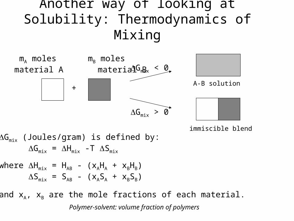
Another way of looking at Solubility: Thermodynamics of Mixing
Gmix < 0
Gmix > 0
immiscible blend
A-B solution
Gmix (Joules/gram) is defined by:Gmix = Hmix -T Smix
where Hmix = HAB - (xAHA + xBHB)Smix = SAB - (xASA + xBSB)
and xA, xB are the mole fractions of each material.
mA moles mB moles material A material B
+
Polymer-solvent: volume fraction of polymers

Ethanol(1) / chloroform(2) at 50ºC
Ethanol(1) / n-heptane(2) at 50ºC
Ethanol(1) / water(2) at 50ºC
Thermodynamics of Mixing: Small Molecules

Solvent-Solvent Solutions vs Polymer-Solvent Solutions
Solvents can easily replace one another.Polymers are thousands of solvent sized monomers connected together. Monomers can not be placed randomly!
• Entropy of mixing is generally positive• Enthalpy is also often positive: smaller the better
Ideal = 0

Flory-Huggins Theory• Flory-Huggins theory, originally derived for small molecule systems, was
expanded to model polymer systems by assuming the polymer consisted of a series of connected segments, each of which occupied one lattice site.
• Assuming segments are randomly distributed and that all lattice sites are occupied, the free energy of mixing per mole of lattice sites is
Gmix=RT[(A/NA)lnA+(B/NB)lnB+FHAB] (3)
i is the volume fraction of polymer i
Ni is the number of segments in polymer i
HF is the Flory-Huggins interaction parameter

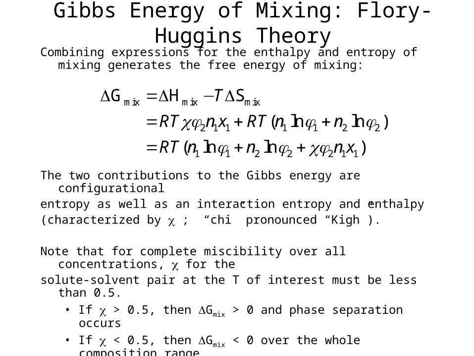
Gibbs Energy of Mixing: Flory-Huggins TheoryCombining expressions for the enthalpy and entropy of mixing generates
the free energy of mixing:
The two contributions to the Gibbs energy are configurationalentropy as well as an interaction entropy and enthalpy(characterized by ; “chi” pronounced “Kigh”).
Note that for complete miscibility over all concentrations, for thesolute-solvent pair at the T of interest must be less than 0.5.
• If > 0.5, then Gmix > 0 and phase separation occurs
• If < 0.5, then Gmix < 0 over the whole composition range.• The temperature at which = 0.5 is the theta temperature.
mix mix mix
2 1 1 1 1 2 2
1 1 2 2 2 1 1
G H S
( ln ln )
( ln ln )
T
RT n x RT n n
RT n n n x
φ φ φφ φ φ
= − = + += + +

For a mixture of polymer and solvent or two polymers
Mixing is always entropically good.
Gibbs Energy of Mixing: Flory-Huggins TheoryCombining expressions for the enthalpy and entropy of mixing generates
the free energy of mixing:
The two contributions to the Gibbs energy are configurationalentropy as well as an interaction entropy and enthalpy(characterized by ; “chi” pronounced “Kigh”).
Note that for complete miscibility over all concentrations, for thesolute-solvent pair at the T of interest must be less than 0.5.
• If > 0.5, then Gmix > 0 and phase separation occurs
• If < 0.5, then Gmix < 0 over the whole composition range.• The temperature at which = 0.5 is the theta temperature.
mix mix mix
2 1 1 1 1 2 2
1 1 2 2 2 1 1
G H S
( ln ln )
( ln ln )
T
RT n x RT n n
RT n n n x
φ φ φφ φ φ
= − = + += + +
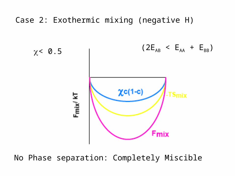
Case 2: Exothermic mixing (negative H)
(2EAB < EAA + EBB) < 0.5
No Phase separation: Completely Miscible
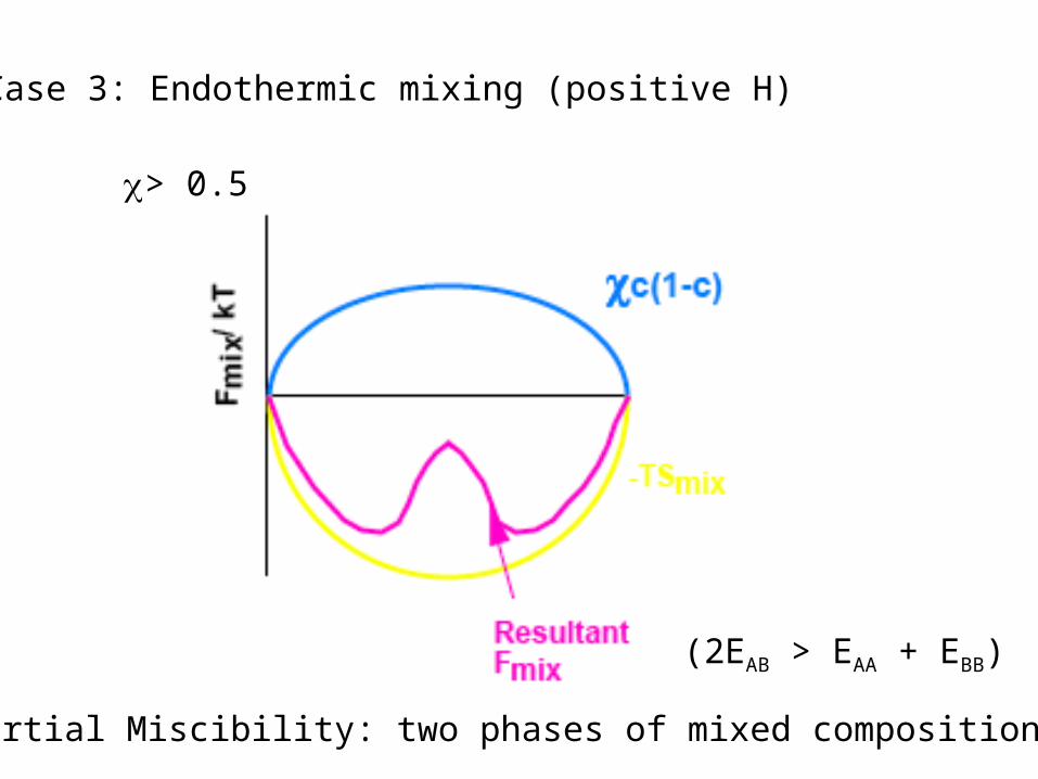
Case 3: Endothermic mixing (positive H)
(2EAB > EAA + EBB)
> 0.5
Partial Miscibility: two phases of mixed compositions
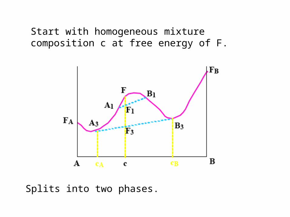
Start with homogeneous mixture composition c at free energy of F.
Splits into two phases.
Blends are not easy to make:
• Blends are not easy to discover-often copolymers are needed to make blend with another homopolymer
• Phase separation gets out of hand in immiscible systems without compatibilizers.
• Some blends must be made with solvent.
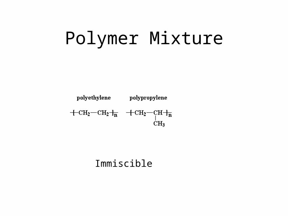
Polymer Mixture
Immiscible

Some miscible blends
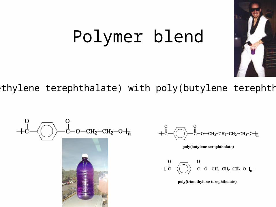
Polymer blend
poly(ethylene terephthalate) with poly(butylene terephthalate)
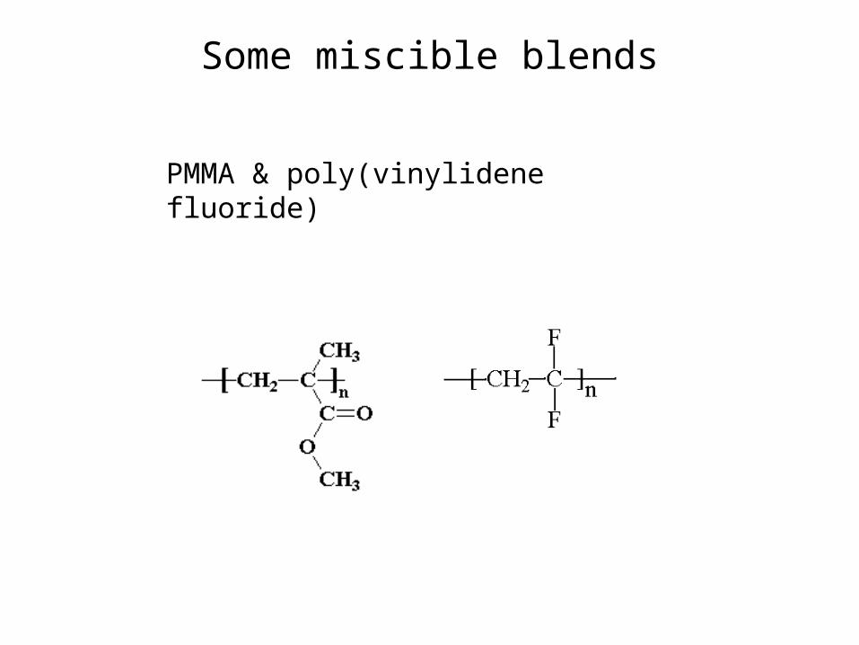
Some miscible blends
PMMA & poly(vinylidene fluoride)

Some miscible blends
Mini Cooper / Cooper S, radiator grille
& PETE
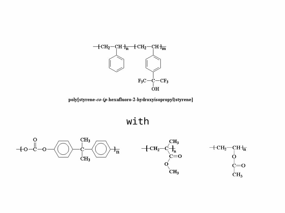
with
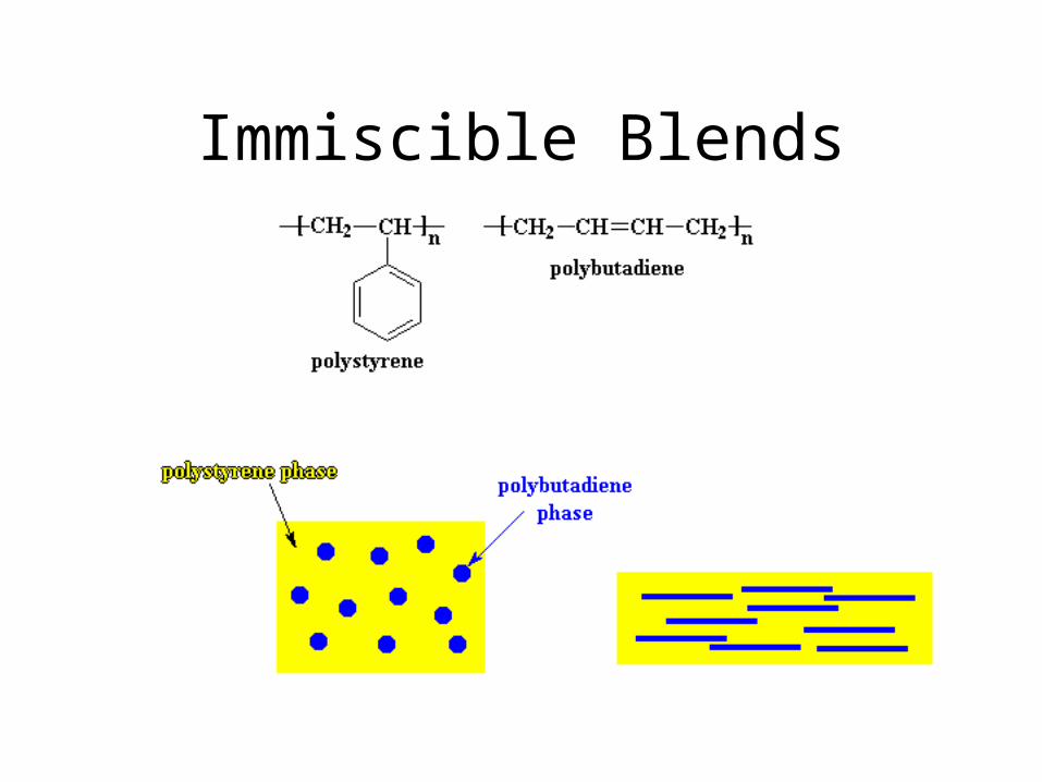
Immiscible Blends


Immiscible Blends
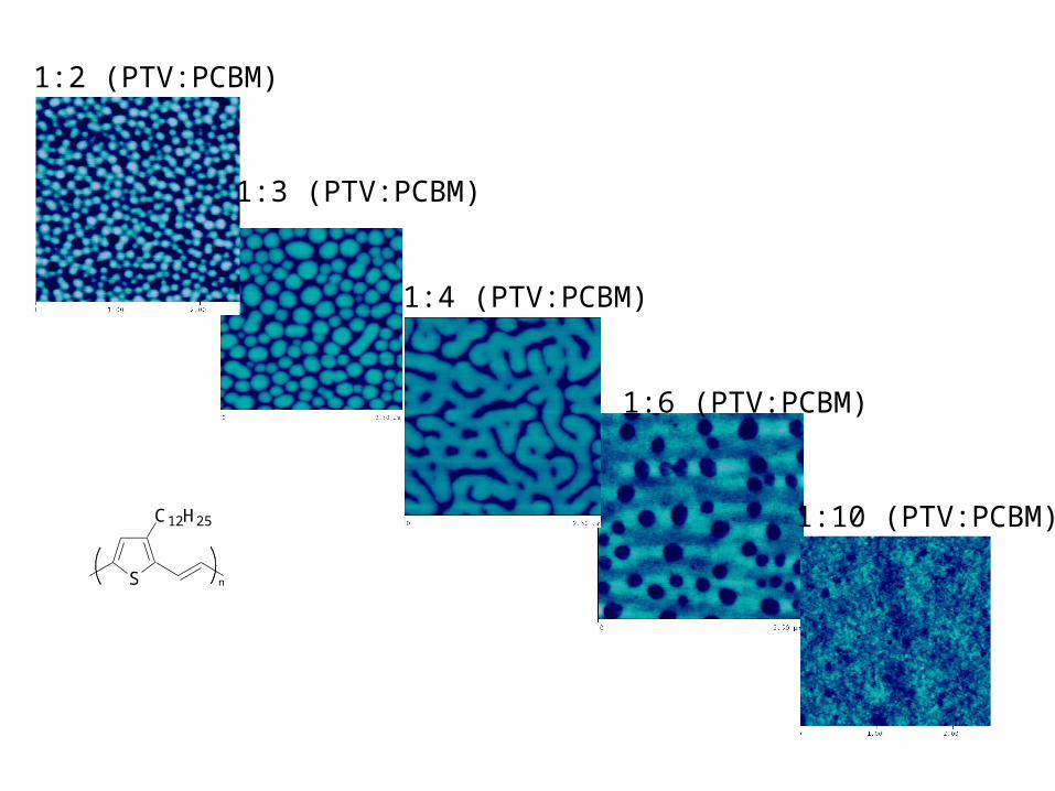
1:6 (PTV:PCBM)
1:4 (PTV:PCBM)
1:3 (PTV:PCBM)
1:2 (PTV:PCBM)
1:10 (PTV:PCBM)
nS
C12H25
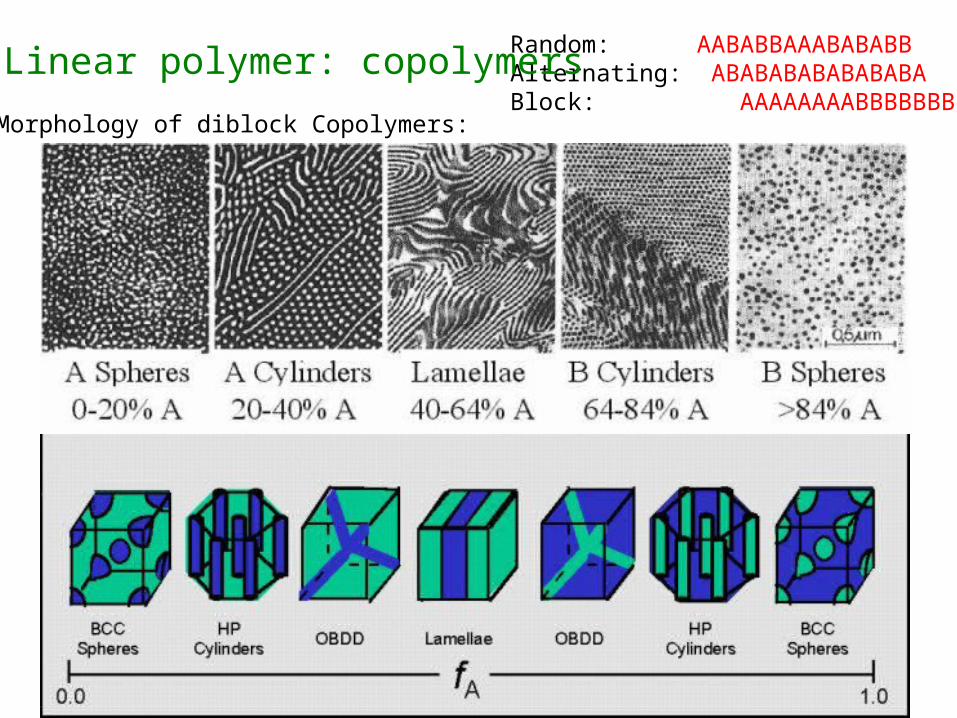
Random: AABABBAAABABABBAlternating: ABABABABABABABABlock: AAAAAAAABBBBBBB
1. Linear polymer: copolymers
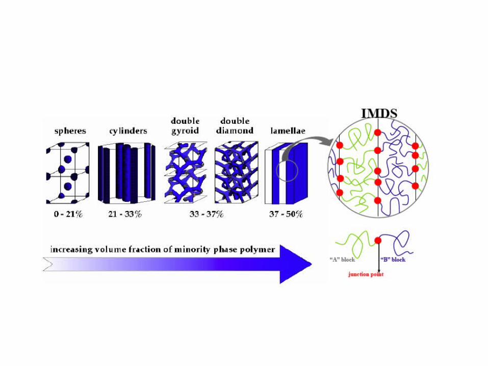
Morphology of diblock Copolymers:

PMMA-PS-PB ternary blend
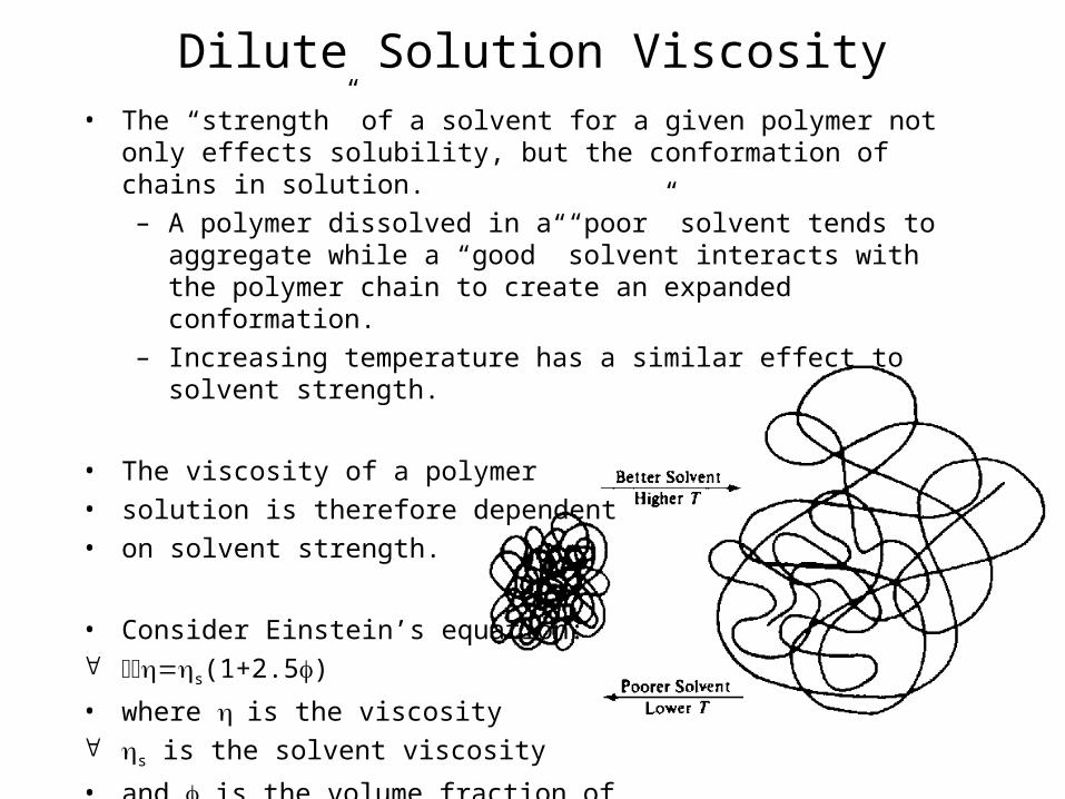
Dilute Solution Viscosity• The “strength” of a solvent for a given polymer not only effects
solubility, but the conformation of chains in solution.
– A polymer dissolved in a “poor” solvent tends to aggregate while a “good” solvent interacts with the polymer chain to create an expanded conformation.
– Increasing temperature has a similar effect to solvent strength.
• The viscosity of a polymer
• solution is therefore dependent
• on solvent strength.
• Consider Einstein’s equation: s(1+2.5)
• where is the viscosity s is the solvent viscosity
• and is the volume fraction of
• dispersed spheres.

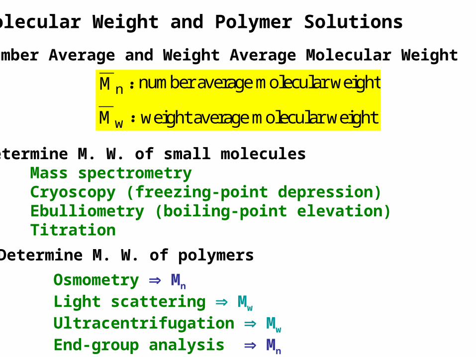
Molecular Weight and Polymer Solutions
Number Average and Weight Average Molecular Weight
Mn number average molecular weight
Mw weight average molecular weight
Determine M. W. of small moleculesMass spectrometryCryoscopy (freezing-point depression)Ebulliometry (boiling-point elevation)Titration
Determine M. W. of polymers
Osmometry Mn
Light scattering Mw
Ultracentrifugation Mw
End-group analysis Mn
Measurement of Number Average Molecular Weight
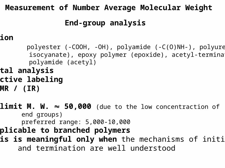
End-group analysis
Titration polyester (-COOH, -OH), polyamide (-C(O)NH-), polyurethanes( isocyanate), epoxy polymer (epoxide), acetyl-terminated polyamide (acetyl)
Elemental analysisRadioactive labelingUV / NMR / (IR)
Upper limit M. W. 50,000 (due to the low concentraction of end groups) preferred range: 5,000-10,000
Not applicable to branched polymersAnalysis is meaningful only when the mechanisms of initiation and termination are well understood

Membrane Osmometry
● based on colligative properties● most useful method for Mn
(range: 50,000 to 2,000,000)● major error source arising from the loss of low MW species ● obtained Mn values are
generally higher than other colligative measurement method
Static equilibrium method measure the hydrostatic head (h) after equilibriumDynamic equilibrium method measure the counter pressure needed to maintain equal liquid levels
h
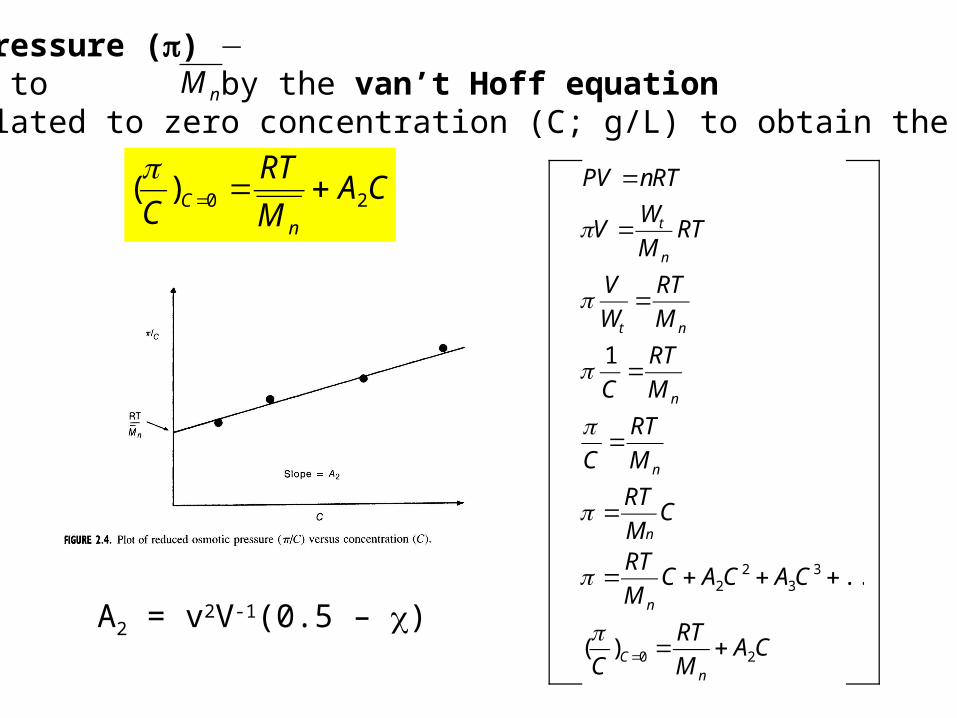
Osmotic pressure () related to by the van’t Hoff equation extrapolated to zero concentration (C; g/L) to obtain the intercept
nM
CAM
RT
Cn
C 20)( +==
CAM
RT
C
CACACM
RT
CM
RT
M
RT
C
M
RT
C
M
RT
W
V
RTM
WV
RTnPV
nC
n
n
n
n
nt
n
t
20
33
22
)(
...
1
+=
+++=
=
=
=
=
=
=
=
A2 = v2V-1(0.5 – )

Cryoscopy and Ebulliometry
Thermodynamic relationships
CAMH
RT
C
T
nfC
f2
2
0
+
=⎟⎟⎠
⎞⎜⎜⎝
⎛
= ρ
CAMH
RT
C
T
nvC
b2
2
0
+
=⎟⎠
⎞⎜⎝
⎛
= ρ
for freezing-point depression
for boiling-point elevation
freezing point or boiling point (solvent)latent heat of fusion (per gram)latent heat of vaporization (per gram)second virial coefficient
T ::::
HfHvA2ρ : solvent density
• Limited by the sensitivity of measuring Tf, Tb
• As MW higher; Tf, Tb smaller• Upper limit - Mn = 40,000• Preferred - Mn < 20,000

Vapor Pressure Osmometry
● For Mn < 25,000● No membrane needed• Thermodynamic principle similar to membrane osmometry
Measurement method → Add a drop of solvent and solution,
on a pair of matched themistors, in an insulated chamber saturated with solvent vapor then, → Condensation heats the solution thermistor (until the vapor pressure of the solution equal to that of the pure solvent)
Temperature change is measured (by resistance change of the thermistor) and related to solution molality
mRT
T ⎟⎟⎠
⎞⎜⎜⎝
⎛=
100
2
λλ : heat of vaporization per gram (solvent)
g
M/W=
g= t
10001000nn
m
m : molarity

Mass Spectrometry
MALDI-MS (MALDI-TOF) MALDI-MS (matrix-assisted laser desorption ionization mass spectrometry) (TOF - time-of-flight)● Imbeds polymer in a matrix of low MW organic compound ● Irradiates the matrix with UV laser ● Matrix transfer the absorbed energy to polymer and vaporize the polymer ● Integrated peak areas the number of ions● Mn, Mw can be calculated
Soft ionization method field desorption (FD-MS) laser desorption (LD-MS) electrospray ionization (ESI-MS)
nM
1
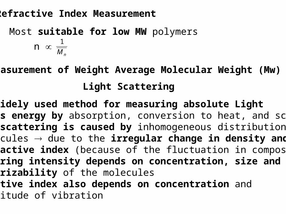
Refractive Index Measurement
Most suitable for low MW polymers
n
Measurement of Weight Average Molecular Weight (Mw)
Light Scattering
• Most widely used method for measuring absolute Light loses energy by absorption, conversion to heat, and scattering• Light scattering is caused by inhomogeneous distribution of molecules due to the irregular change in density and refractive index (because of the fluctuation in composition)• Scattering intensity depends on concentration, size and polarizability of the molecules• Refractive index also depends on concentration and amplitude of vibration

LS adds optical effects Size
q = 0 in phase Is maximum
q > 0 out of phase, Is goes down 3
122g
s
RqI −≅
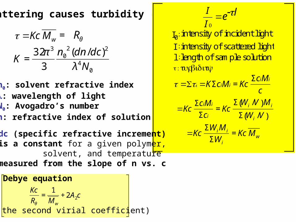
Scattering causes turbidity ()
€
=Kc Mw
€
K =32π 3
3
n02(dn /dc)2
λ4N0
leI
I -0=
€
=Σi =KΣciMi = KcΣciMi
c
€
=KcΣciMi
Σci= Kc
Σ W i /V( )M i
Σ W i /V( )
€
=KcΣW iM i
ΣW i
= Kc Mw
I0: intensity of incident light
I : intensity of scattered lightl : length of sample solution : turbidity
n0: solvent refractive index λ: wavelength of lightN0: Avogadro’s number n: refractive index of solution
dn/dc (specific refractive increment)• is a constant for a given polymer, solvent, and temperature• measured from the slope of n vs. c
€
Kc
Rθ
=1
Mw
+ 2A2c
Debye equation
(A2: the second virial coefficient)
=
€
Rθ

As molecular size approaches the wavelength of the light
• Interference between scattered light coming from different parts occurs• Correction is needed
Turbidity ( or R) associated with large particles• measured at different concentrations (c) and angles ()
€
Kc
ΔRθ
=1
MwP(θ )+ 2A2c
⎡
⎣ ⎢
⎤
⎦ ⎥ P(): Particle scattering factor
P() is a function of ; depending on the shape of molecule in solution
For a monodisperse of randomly coiling polymers
)]1()[2
()(2
vev
P v −−= −
)2
(sin))(16( 22
2
2 λ
s
sv=
ns
λλ =
s 2: mean-square radius of gyration of the molecue
λs: the wavelength in solution

Zimm Plot
Plot
€
Kc
Rθ
⎛
⎝ ⎜
⎞
⎠ ⎟ vs. [sin2(/2)+kc] k is an arbitrary constant
Extrapolated to both zero concentration and zero angle intercept =
wM
1 (P() = 1 at c = 0 and = 0)
€
Kc
Rθ
⎛
⎝ ⎜
⎞
⎠ ⎟
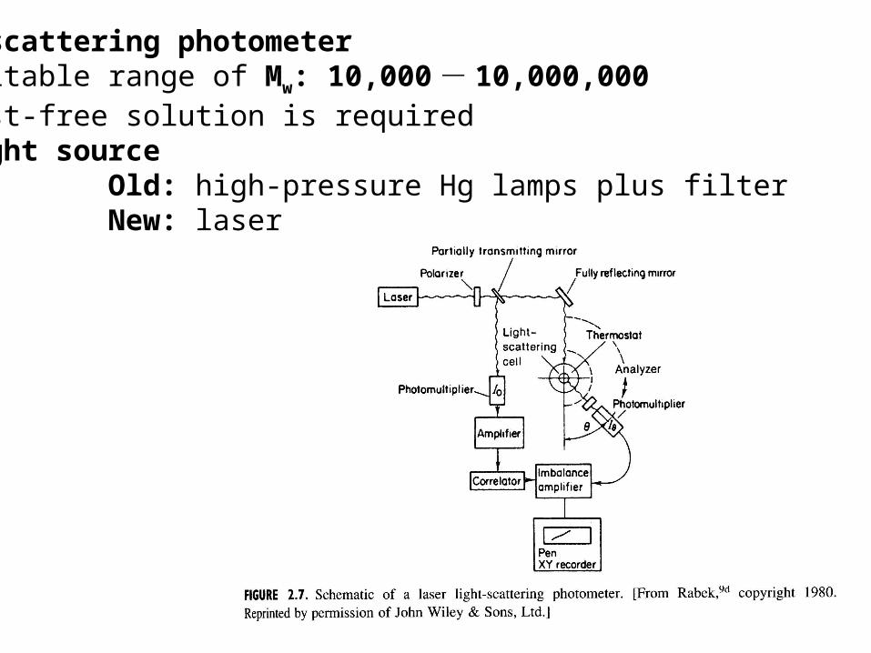
Light scattering photometer• Suitable range of Mw: 10,000 - 10,000,000• Dust-free solution is required• Light source Old: high-pressure Hg lamps plus filter New: laser
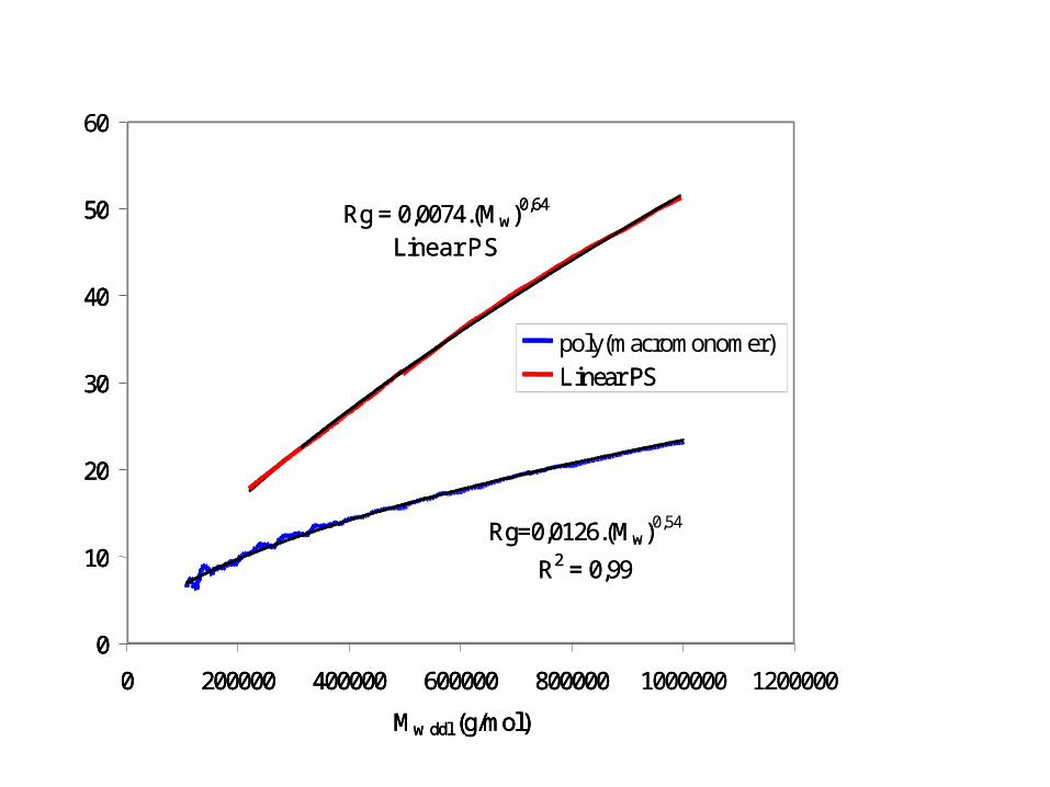
0,54
60
1000000 1200000
poly(macromonomer)
Rg=0,0126.(Mw)
R2 = 0,99
Rg = 0,0074.(Mw)0,64
Linear PS
0
10
20
30
40
50
0 200000 400000 600000 800000
Mw ddl (g/mol)
Rg
(nm)Linear PS
0,54
60
1000000 1200000
poly(macromonomer)
Rg=0,0126.(Mw)
R2 = 0,99
Rg = 0,0074.(Mw)0,64
Linear PS
0
10
20
30
40
50
0 200000 400000 600000 800000
Mw ddl (g/mol)
Rg
(nm)Linear PS
Rg=0,0126.(Mw)
R2 = 0,99
Rg = 0,0074.(Mw)0,64
Linear PS
0
10
20
30
40
50
0 200000 400000 600000 800000
Mw ddl (g/mol)
Rg
(nm)Linear PS
zM
• Most expensive• Extensively used with proteins• Determining
Ultracentrifugation
• Sedimentation rate is proportional to molecular mass• Distributed according to size along the perpendicular direction• Concentration gradients within the polymer solution are observed by refractive index measurements and interferometry
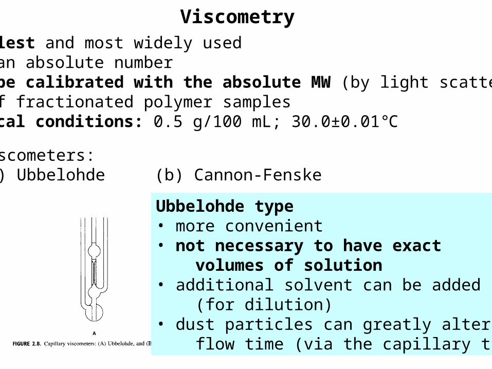
• Simplest and most widely used• Not an absolute number• Can be calibrated with the absolute MW (by light scattering) of fractionated polymer samples• Typical conditions: 0.5 g/100 mL; 30.0±0.01℃
Viscometry
Viscometers:(a) Ubbelohde (b) Cannon-Fenske
Ubbelohde type• more convenient• not necessary to have exact volumes of solution• additional solvent can be added (for dilution)• dust particles can greatly alter the flow time (via the capillary tube)
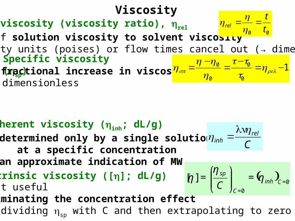
Relative viscosity (viscosity ratio), rel ● ratio of solution viscosity to solvent viscosity● viscosity units (poises) or flow times cancel out (→ dimensionless)
Viscosity
00 t
trel ==
Specific viscosity (sp) ● fractional increase in viscosity● dimensionless
10
0
0
0 −=−
=−
= relsp ttt
Inherent viscosity (inh; dL/g)● determined only by a single solution at a specific concentration● an approximate indication of MW
Crel
inh
ln=
Intrinsic viscosity ([]; dL/g)● most useful● eliminating the concentration effect● by dividing sp with C and then extrapolating to zero C
( ) 0
0
][ =
=
=⎟⎟⎠
⎞⎜⎜⎝
⎛= Cinh
C
sp
Cη
ηη

00 t
trel ==
1
0
0
0
0 −=−
=−
= relt
ttsp
C
rel
C
spred
1−==
C
relinh
ln=
0)(
0
][ ===
= ⎟⎟⎠
⎞⎜⎜⎝
⎛Cinh
CC
sp
Common Name IUPAC Name
Relative viscosity Viscosity ratio
Specific viscosity -
Reduced viscosity Viscosity number
Inherent viscosityLogarithmic viscositynumber
Intrinsic viscosityLimiting viscosity number
Table 2.2. Dilute Solution Viscosity Designationsa
aConcentrations (most commonly expressed in grams per 100 mL of solvent) of about 0.5 g/dL
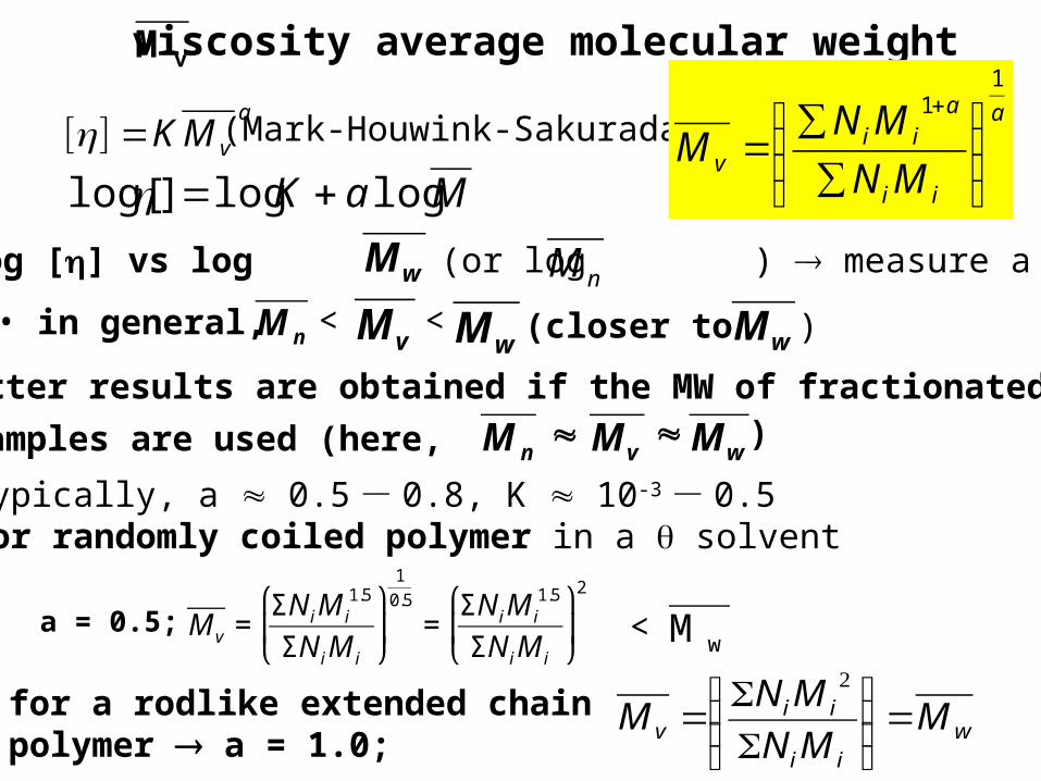
vM viscosity average molecular weight
a
vMK=][ (Mark-Houwink-Sakurada) a
ii
aii
v MN
MNM
11
⎟⎟⎠
⎞⎜⎜⎝
⎛
∑∑
=+
MaK loglog]log[ +=• plot log [] vs log (or log ) measure a and K
nMwM
• in general, nMvM wM< < (closer to wM )
• better results are obtained if the MW of fractionated
samples are used (here, nM vM wM
)
● typically, a 0.5 - 0.8, K 10-3 - 0.5● for randomly coiled polymer in a solvent
a = 0.5;
€
Mv =ΣN iM i
1.5
ΣN iM i
⎛
⎝ ⎜
⎞
⎠ ⎟
1
0.5
=ΣN iM i
1.5
ΣN iM i
⎛
⎝ ⎜
⎞
⎠ ⎟
2
wM<
• for a rodlike extended chain polymer a = 1.0; w
ii
iiv M
MN
MNM =⎟⎟
⎠
⎞⎜⎜⎝
⎛
ΣΣ
=2
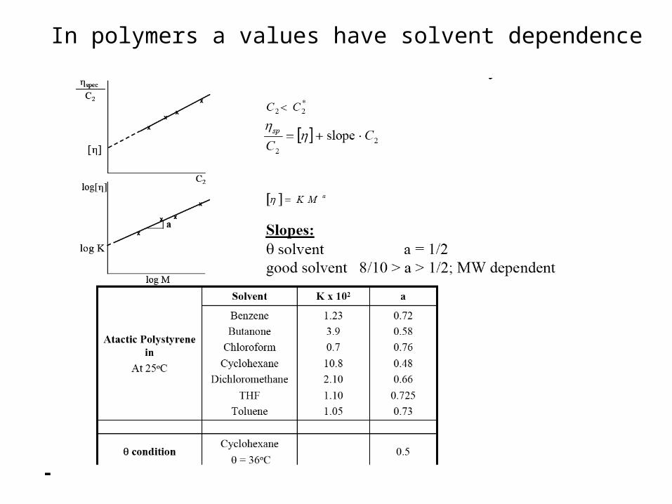
In polymers a values have solvent dependence
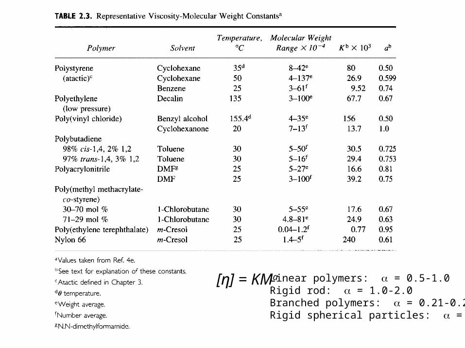
[η] = KMa Linear polymers: = 0.5-1.0Rigid rod: = 1.0-2.0Branched polymers: = 0.21-0.28Rigid spherical particles: = 0
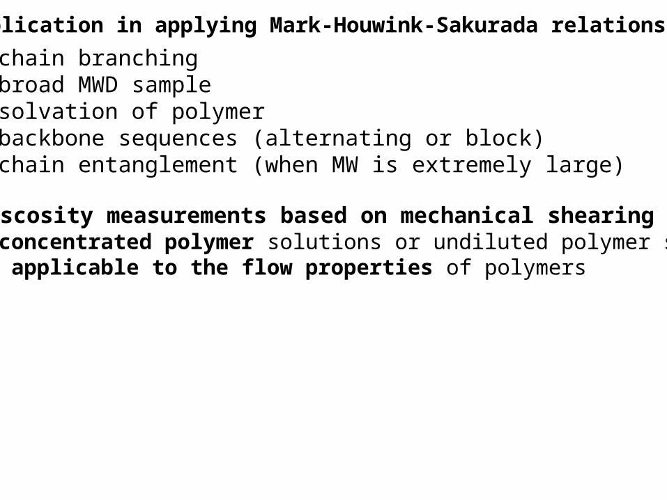
Complication in applying Mark-Houwink-Sakurada relationship
• chain branching• broad MWD sample• solvation of polymer • backbone sequences (alternating or block)• chain entanglement (when MW is extremely large)
Viscosity measurements based on mechanical shearing • for concentrated polymer solutions or undiluted polymer system• more applicable to the flow properties of polymers

Dynamic Viscosity
Viscosity = Pa s = kg m s-1
Force/Area = Pa m-1 = kg m-1 s-2
Force: Pa = N m-2 = kg m s-2
1 Pa s = 10 Poise1 centipoise = 1 millipascal second (mPa s)
Other units (Poise = dyne s cm-2)
Informally: resistance to flowFormally: Ratio of Shearing stress (F/A) to the velocity gradient (dvx/dz)
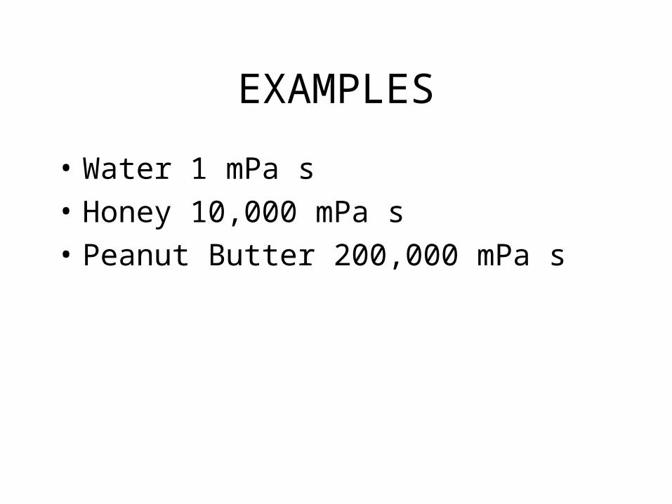
EXAMPLES
• Water 1 mPa s
• Honey 10,000 mPa s
• Peanut Butter 200,000 mPa s

Kinematic viscosity is the dynamic viscosity divided by the density (typical units cm2/s, Stokes, St).
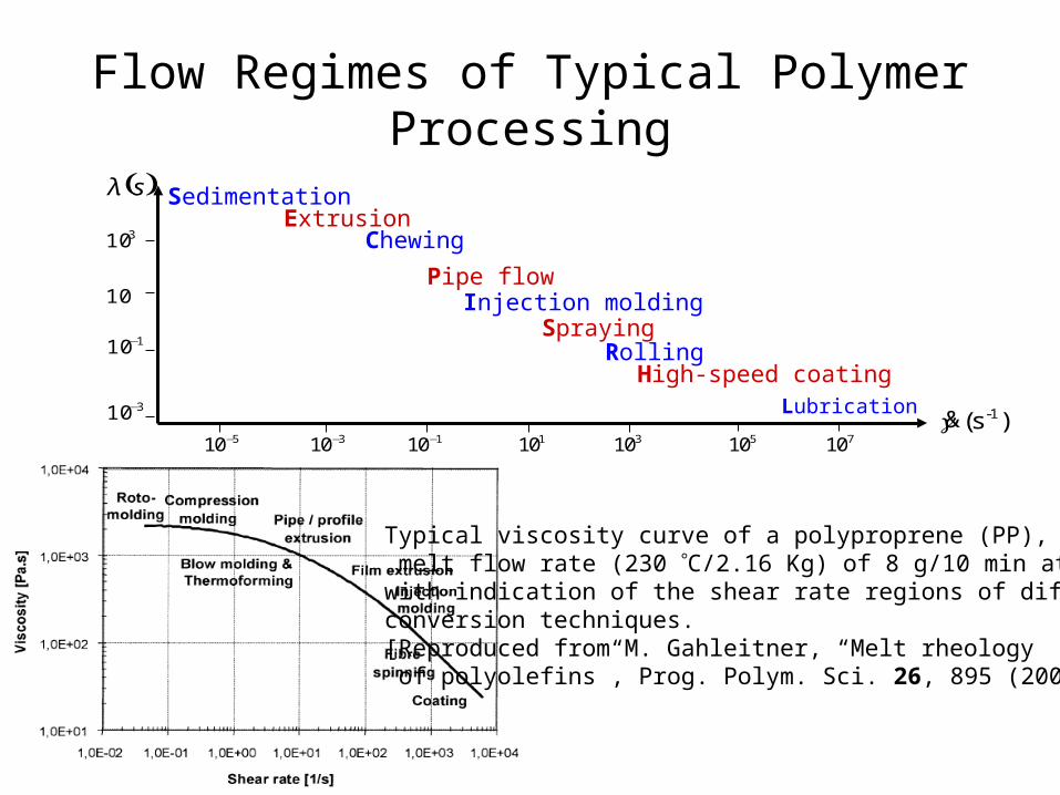
Flow Regimes of Typical Polymer Processing
310−
110−
10
-1 ( )γ& s
High-speed coating
Injection molding
Lubrication
Sedimentation
Rolling
Pipe flow
Extrusion
Spraying
Chewing
710510310110110−310−510−
( )sλ
310
Typical viscosity curve of a polyproprene (PP), melt flow rate (230 C/2.16 Kg) of 8 g/10 min at 230 C with indication of the shear rate regions of different conversion techniques. [Reproduced from M. Gahleitner, “Melt rheology of polyolefins”, Prog. Polym. Sci. 26, 895 (2001).]