Embed Size (px)
Citation preview

Technische Universität Berlin
Institut für Chemie
Polymerization Technology
Karl-Heinz Reichert Reinhard Schomäcker
Third Edition SS 2017

Preface
This teaching booklet has been written for students attending the Master
Program of Polymer Science, established as a joint program by four universities
in the cities of Berlin and Potsdam.
This text book focuses on fundamental aspects of polymerization reaction
engineering. In the development of a polymerization process the type of reactor
and its mode of operation are key factors, which not only affect reactor
performance and safety, but also to a large extend the quality of the polymeric
product. This is due to the fact that polymers are non uniform materials and the
degree of non uniformity is affected by chemistry and reaction engineering
conditions as well. I hope that the contents of this text book will be of help to
those students who will be envolved in large scale synthesis of polymers in
times to come.
I would like to thank my secretary Veronika Schott for writing the manuscript of
this booklet and especially for her patience with respect to numerous changes of
the text, which I have made all the time.
Thanks also go out to Monika Klein, who drew all the figures presented in this
book and Scott Kibride who improved the English language.
Finally we would like to thank all my former PhD students and many of our
colleagues for some of their scientific results, which we have used in this text
book.
Karl Heinz Reichert Berlin in October 2002
Reinhard Schomäcker Berlin in April 2017

TABLE OF CONTENTS
1. Introduction 1
1.1 Classification of Polymers 1
1.2 Types of Polymerization Reactions 2
1.3 Methods of Polymerization 3
1.4 Types of Polymerization Reactors 4
1.5 General References 4
1.6 Tables and Figures 6
2. Kinetics of Polymerization and Molecular Weight of Polymers 9
2.1 Free Radical Polymerization in Solution 9
2.1 Free Radical Polymerization in Emulsion 16
2.3 Free Radical Copolymerization in Solution 23
2.4 Coordination Polymerization in Gas Phase 24
2.5 Coordination Polymerization in Liquid Phase 32
2.6 List of Symbols 34
2.7 References 35
2.8 Tables and Figures 37
3. Viscosity of Reaction Mixture 55
3.1 Introduction 55
3.2 Viscosity of Homogeneous Systems 55
3.3 Viscosity of Heterogeneous Systems 58
3.4 List of Symbols 59
3.5 References 60
3.6 Figures 61
4. Data Acquisition of Polymerization Reactions 66
4.1 Introduction 66
4.2 Reaction Calorimetry/Kinetic and Caloric Data 66
4.3 Reaction Viscosimetry/Rheological Data 70
4.4 Solubility and Diffusivity of Monomer in Polymer 71
4.5 List of Symbols 73
4.6 References 74
4.7 Figures 75
5. Polymerization in Stirred Tank Reactors 83
5.1 Mode of Operation 83

5.2 Mixing of Reaction Mixture 84
5.3 Heat Removal and Safety Aspects 92
5.4 Residence Time Distribution 98
5.5 Reactor Performance 101
5.6 Reactor Selectivity 105
5.7 Reactor Scale-up 109
5.8 List of Symbols 111
5.9 References 113
5.10 Tables and Figures 114
6. Polymerization Processes 139
6.1 General Aspects 139
6.2 Processes for Chain-Growth Polymerization 140
Solution Polymerization/High Density Polyethylene
Suspension Polymerization/Poly(vinyl chloride)
Emulsion Polymerization/Styrene-Butadiene-Copolymer
Slurry Polymerization/High Density Polyethylene
Gas Phase Polymerization/High Density Polyethylene
6.3 Processes for Step-Growth Polymerization 146
Condensation Polymerization in Solution/Phenolic Resins
Condensation Polymerization in Melt and Solid State/Poly-
(ethylene terephthalate)
Addition Polymerization in Liquid Phase/Polyurethanes
6.4 References 149
6.5 Tables and Figures 150


1
1. INTRODUCTION
1.1 Classification of Synthetic Polymers
Synthetic polymers can be classified according to their specific properties into
thermoplastics, thermosets and elastomers. Examples of major polymers of each
kind are listed in Tab. 1.1.
Thermoplastic polymers are organic materials, which consist of linear or
branched macromolecules having molecular weights on the order of 100 000
gram per mole. On heating above melting point thermoplastic polymers melt and
form highly viscous liquids with a typical flow pattern. On cooling the melt
solidifies again. In this way thermoplastic polymers can easily be processed into
materials of different shapes. According to the physical structure and chemical
composition of the polymers they can be partially crystalline or amorphous
materials in the solid state. Amorphous polymers like polyvinyl chloride, poly-
styrene, and polyesters are transparent materials. Partially crystalline polymers
like high density polyethylene and polypropylene are not transparent in the solid
state due to their heterophasic structure.
Thermosets are organic materials, which are formed by higly crosslinked macro-
molecules with extremely high molecular weights. On heating they can not be
molten but they do decompose and lose their original properties. Therefore
thermosets have to be processed in such a way that synthesis and processing of
the polymer material is done at the same time in a given cavity corresponding to
the shape of the material which is to be produced. In general, thermosets are
filled with glass fibre to improve the mechanical strengh of the materials.
Elastomers are linear or branched macromolecules which are very flexible. The
molecules contain double bonds, which can easily react with added crosslinker
at elevated temperatures, forming a crosslinked material with rubber-like
properties.
Typical properties of organic polymers are low specific weight, low heat and
electrical conductivity, and good resistant to corrosion. Feedstocks for major
polymers are crude oil, natural gas, salt, air, and water. Organic polymers are
produced by a relatively small number of large chemical companies. Approxi-
mately seventy percent of all polymers produced are thermoplastics, twenty
percent are thermosets, and ten percent are elastomers.

2
1.2 Types of Polymerization Reactions
Polymerization reactions can be very complex chemical reactions with many
different side reactions. One way of classification of polymerization reactions is
to look at the polymer growth reaction, which is essential for polymer formation.
By looking at the polymer growth reaction, chainwise and stepwise poly-
merization reactions can be distinguished. See Tab. 1.2.
In chainwise polymerization reactions the propagation of a molecule happens by
the consecutive addition of bifunctional monomer molecules (M) to an active
site ( *nP ) of chain length n. Once the active sites are formed they start a chain of
monomer addition reactions until the chain is terminated by a termination
reaction. The active sites can be free radicals, organo metallic complexes or
anionic or cationic species of very different kinds. Depending on the nature of
active sites polymerization reactions can be classified into free radical
polymerization, coordination polymerization, and ionic polymerization. If these
polymerization reactions do not have any chain termination or chain transfer
reaction they are called living polymerization. In case of a living polymerization
the life time of active sites are long (at least on the order of total reaction time).
The life time of free radicals is in general on the order of seconds. Active sites
of organo metallic catalysts can have very different life times. In general they
are on the order of seconds or minutes. The concentration of active sites of
chainwise polymerization reactions is in general very low and it can be constant
or non-constant with conversion of monomer in batchwise reaction. As
mentioned before, chainwise polymerization reactions are complex reactions
consisting of initiation, propagation, termination and transfer reactions. All of
the reactions are running simultaneously. The molecular weight of polymers
formed during chainwise polymerization can remain constant or decrease or
increse with conversion of monomer. This depends on the contribution of each
single reaction. In case of a free radical polymerization run in a batch reactor at
constant temperature the molecular weight remains constant with conversion if
chain transfer reactions play a dominant role. If not, it will fall with conversion
due to decreasing concentration of monomer. The same is true for coordination
polymerization. In case of living polymerization the molecular weight of
polymer formed is increasing with conversion in any case since no termination
and transfer reactions are present in the reacting system. The molar
concentration of polymer molecules of chainwise polymerization reactions also
depends on the kind of polymerization. It remains constant with conversion for a
living polymerization and is increasing for free radical and coordination
polymerization since at any time new polymer molecules are formed.
The situation can be quite different in the case of stepwise polymerization
reactions. Here the polymer growth reaction takes place by stepwise reactions of
bifunctional molecules (Pn and Pm in Tab 1.2). The molecules can be monomers,

3
oligomers, or polymers depending on the degree of conversion. At the beginning
of reaction only monomer molecules are present in the reaction mixture. With
increasing conversion monomer concentration is rapidly falling and oligomers
are formed. High molecular weight polymers are only formed at very high
conversion of functional groups (above 99 %). The polymer growth reaction is a
typical condensation reaction like the reaction of carboxylic groups with
hydroxylic groups; forming ester groups and water. This kind of polycon-
densation reactions are in general reversible reactions, which have to be shifted
to the right side of the equilibrium for high conversions. The active sites are the
functional groups of the reacting molecules, with an infinite life time on its own.
The concentration of functional groups is decreasing with increasing conversion.
In an ideal case there are no other side reactions in stepwise polymerization
reactions beside growth reaction. The avarage molecular weight of the
condensation products increases with conversion of functional groups. First
there is a very slow increase, then at high conversion there is a very strong
increase in molecular weight. High molecular weight polycondensates can only
be achieved at very high conversions. The molar concentration of polymer
molecules decreases with conversion. At a conversion of 100% only one huge
macromolecule should be present in the reaction volume.
The most industrially important polymers listed in Tab. 1.1 are produced by free
radical polymerization (ethylene, vinylchloride, styrene, butadiene) by coordi-
nation polymerization (ethylene, propylene, butadiene) and by condensation or
addition polymerization (polyesters, polyurethanes, formaldehyde resins).
1.3 Methods of Polymerization
Polymerization reactions are highly exothermic reactions, producing a large
amount of heat that has to be removed from the reaction medium.
Polymerization reactions are further characterized by a very strong increase of
viscosity of the reaction mixture with conversion, which can cause problems
with mixing, heat removal, and transport of the reaction mixture. Another
characteristic feature of polymerization reactions is the sensitivity of the reaction
rate to very small amounts of impurities, such as free radical scavangers or
catalyst poisons. These impurities have to be removed by very intensive
cleaning of the reactants and solvents before starting the reaction.
Polymerization reactions can be performed in very different ways. In Tab. 1.3
different methods of performing polymerization reactions are listed. The
reaction medium can either be a homogeneous or a heterogeneous system.
Heterogeneous systems have the great advantage of having a much lower
viscosity than the corresponding homogeneous system at equivalent conditions.
Due to this advantage mixing, heat removal, and transport is not as much of a
problem as it is in the case of homogeneous systems. The decision of which

4
process is to be used for performing a polymerization reaction does not only
depend on the engineering aspects named, but also on the properties of the
polymer to be produced and the method of polymer processing for
manufacturing of the polymeric material. For example polyethylene can be
produced by free radical polymerization in bulk phase at super critical
conditions (low density polyethylene for films), but also by coordination
polymerization in a slurry or gas phase (high density polyethylene for pipes and
containers).
1.4. Types of Polymerization Reactors
Major polymerization reactors used in industry are represented schematically in
Fig. 1.1. The type of reactor used depends mainly on the method of polymeri-
zation. Most polymerization reactions are run in liquid phase, with some in gas
phase. The most widely used reactor for liquid phase polymerization is the
stirred tank reactor. It is used for batch, semibatch and continuous processes. In
case of continuous processes the stirred tank reactor is used as a single reactor or
as a cascade of stirred tank reactors. A single stirred tank reactor has a very
broad residence time distribution while a cascade of stirred tank reactors is
characterized by a more narrow residence time distribution. This may affect
performance and selectivity of the reactor. In the case of gas phase
polymerization reactions the fluidized bed reactor is used in general. It is run
continuously and has a very broad residence time distribution. Tubular reactors
are used for polymerization in liquid phase. In general they are characterized by
a rather narrow residence time distribution. The mode of operation of a reactor
or process is determined mainly by the amount of polymer which has to be
produced. Commodity polymers are produced in continuous processes. Speci-
ality polymers are mostly produced batch- or semibatch-wise.
1.5 General References
- "Comprehensive Polymer Science“, 7 Volumes, G. Allen, J. Bevington
(Eds.), Pergamon Press, 1989
- “Encyclopedia of Polymer Science and Engineering“, 19 Volumes, H.F.
Mark, N.M. Bikales, C.G. Overberger, G. Menges (Eds.), John Wiley and
Sons, 1990
- “Ullmann´s Encyclopedia of Industrial Chemistry“, Vol. A 20, A 21,
A 22, A 23, VCH, 1992
- A. Rudin: “The Elements of Polymer Science and Engineering“, Academic
Press, 1982
- J.A. Biesenberger, D.H. Sebastian: “Principles of Polymerization Enginee-
ring“, John Wiley and Sons, 1983

5
- G. Odian: “Principles of Polymerization“, John Wiley and Sons, 1991
- N.A. Dotson, R. Galván, R.L. Laurence, M. Tirrell: “Polymerization Process
Modelling“, VCH Publishers, 1996
- K.H. Reichert, H.-U. Moritz: “Polymer Reaction Engineering“, in Compre-
hensive Polymer Science, Vol. 3, p. 327, Pergamon Press, 1989
- H.G. Elias: “Plastics, General Survey“, in Ullmanns´s Encyclopedia of
Industrial Chemistry, Vol. A 20, p. 543, VCH, 1992
- A. Hamielec, H. Tobita: “Polymerization Processes“, in Ullmann´s Ency-
clopedia of Industrial Chemistry, Vol. A 21, p. 305, VCH, 1992

6
1.6 Tables and Figures
Thermoplastics Thermosets Elastomers
- Polyethylene
- Polypropylene
- Poly(vinyl chloride)
- Polystyrene and Styrenics
- Poly(ethylene terephthalate)
- Phenol-Formaldehyde-
Resins
- Polyurethanes
- Urea-Formaldehyde-
Resins
- Styrene-Butadiene-
Copolymers
- Polybutadiene
Tab. 1.1: Classification and examples of major synthetic polymers
Chainwise
Polymerization
Stepwise
Polymerization
Polymer growth reaction
1nn PMP XPPP mnmn
Active sites Free radicals
Organometallics
Ions
Functional groups
Specific name of
polymerization reaction
Free radical polymeri-
zation (FRP)
Coordination polymeri-
zation (CP)
Living polymerization
(LP)
Polycondensation or
Polyaddition
Life time of active sites Short for FRP and CP
Long for LP Long
Concentration of
active sites
Low and nearly constant
with conversion for FRP
and LP
Low and non-constant
with conversion for CP
According to monomer
concentration and decrea-
sing with conversion
Other reactions besides
growth reaction
Initiation (FRP, CP, LP)
Termination (FRP, CP)
Transfer reaction
(FRP,CP)
None (ideal case)
Molecular weight
with conversion
Nearly constant for FRP
and CP
Increasing for LP
Increasing
Polymer concentration
with conversion
Constant for LP, increa-
sing for FRP and CP Decreasing
Tab. 1.2: Types of polymerization reactions and characteristic features

7
Solution Polymerization
Polymerization of monomer in presence of a
solvent
Homogeneous system
Bulk Polymerization
Polymerization of monomer in absence of a
solvent (only monomer)
Homogeneous or heterogeneous system
Suspension Polymerization
Polymerization of liquid monomer droplets dis-
persed in a liquid phase (water) using oil soluble
initiators and water soluble surfactants
Emulsion Polymerization
Polymerization of monomer in latex particles
dispersed in a liquid phase (water) using water
soluble initiators and surfactants
Slurry Polymerization
Polymerization of gaseous monomer in catalyst/
polymer particles dispersed in a liquid phase
(gas/solid/liquid system)
Gas Phase Polymerization Polymerization of gaseous monomer in catalyst/
polymer particles dispersed in gas phase
Precipitation
Polymerization
Polymerization of monomer in solution and
precipitation of the polymer formed during
polymerization
Tab. 1.3: Methods of polymerization

8
Fig. 1.1: Schematic representation of major types of polymerization reactors
with broad and narrow residence time distribution

9
2. KINETICS OF POLYMERIZATION AND MOLECULAR
WEIGHT OF POLYMERS
2.1 Free Radical Polymerization in Solution
Rate and Conversion of Polymerization
Free radical polymerization is still the most widely used type of polymerization
for polymer production. It can be run in solution, bulk, suspension, and
emulsion. The reaction scheme of a typical free radical polymerization reaction
is shown in Tab.2.1. The main steps of the reaction are initiation of a chain,
propagation of the chain, termination of the chain, and different kinds of transfer
reactions. In the initiation reaction the initiator decomposes into two primary
radicals which can start a growing chain by addition of a monomer like ethylene,
vinyl chloride or styrene. The additon of the first monomer molecule to a
primary radical can in general not be distinguished from the addition of the
second or third monomer molecule, at least from a kinetic point of view. The
initiation reaction is followed by the chain propagation reaction. In this reaction
many monomer molecules are added to the growing chain. The number of added
monomer molecules is in the order of 1000. Molecules with free radical
character are very reactive species which also can react with each other. In this
case the chain propagation reaction is terminated. Two different kinds of chain
termination reactions have to be considered, with chain termination by
recombination being more common than termination by disproportionation.
Both ways of termination can happen simultaneously. The result of termination
by recombination is the formation of one macromolecule with a much larger
chain length than that of the two original molecules. Termination by dispro-
portionation leads to formation of two macromolecules of the same chain length
as the original active molecules. One of the two molecules formed has a double
bond at the end of the chain and is able to act as a comonomer forming branched
macro molecules. Atom abstraction reactions like abstraction of hydrogen or
halogen atoms in free radical polymerization reactions are called chain transfer
reactions. The atom donor molecule itself (monomer, polymer, solvent, transfer
agent) becomes a radical, and the kinetic chain is not terminated if the new
radical formed can add further monomer molecules. In this case chain transfer
reactions do not affect the kinetics, but only the chain length of the polymer
molecules. To control the molecular weight of polymers effective chain transfer
agents like mercaptanes are added to the reaction medium.
For a free radical polymerization reaction the following kinetic equations can be
derived by making some assumptions. One important assumtion is the quasi-
stationary state assumptions for concentration of free radicals.
10
)]sl/(mol[CCkdt
dCR M
1/2I
M
2
E
2
EEE;
T
EexpAk;
k
kfkk td
p
1/2
t
dp
R
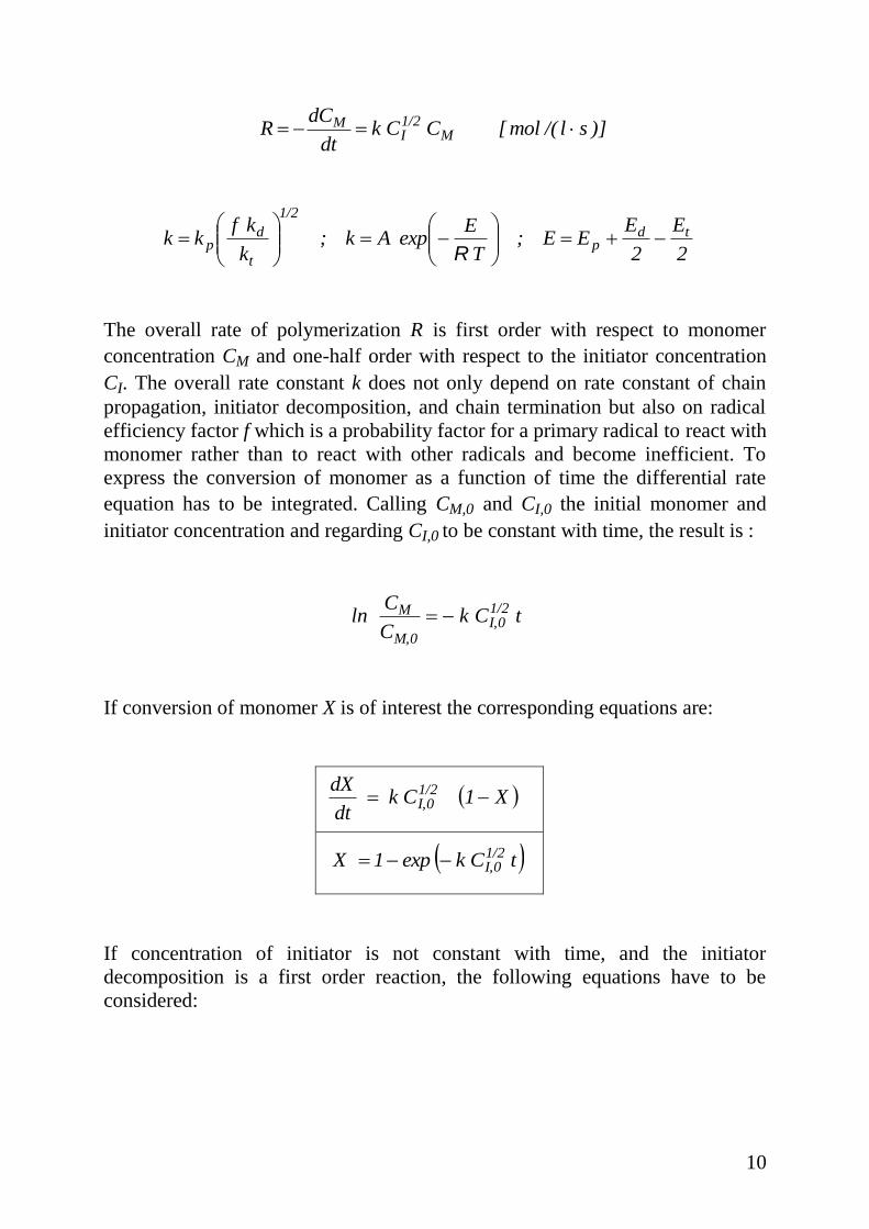
The overall rate of polymerization R is first order with respect to monomer
concentration CM and one-half order with respect to the initiator concentration
CI. The overall rate constant k does not only depend on rate constant of chain
propagation, initiator decomposition, and chain termination but also on radical
efficiency factor f which is a probability factor for a primary radical to react with
monomer rather than to react with other radicals and become inefficient. To
express the conversion of monomer as a function of time the differential rate
equation has to be integrated. Calling CM,0 and CI,0 the initial monomer and
initiator concentration and regarding CI,0 to be constant with time, the result is :
tCkC
Cln 1/2
I,0M,0
M
If conversion of monomer X is of interest the corresponding equations are:
X1Ckdt
dX 1/2I,0
tCkexp1X 1/2I,0
If concentration of initiator is not constant with time, and the initiator
decomposition is a first order reaction, the following equations have to be
considered:

11
X1t2
kexpCk
dt
dX d1/2I,0
1t
2
kexp
k
Ck2exp1X d
d
1/2I,0
The maximum conversion of monomer which can be achieved depends on the
type and concentration of initiator used. If the initiator is decomposing too fast
at reaction conditions than the polymerization reaction stops at a conversion
smaller than 1. This kind of polymerization is called dead-end polymerization.
The maximum conversion of monomer can be calculated by the following
equation:
d
1/2I,0
maxk
Ck2exp1X
For calculation of rate or conversion of free radical polymerization as a function
of time the rate constants are needed. In Tab. 2.2 some suggested values of rate
constants and corresponding activation energies are given. They can strongly
differ and depend on the kind of monomer, initiator, or solvent used. The
numerical value of the chain transfer constant cited in Tab. 2.2 refers to transfer
reactions of monomer, solvent, or polymer but not of transfer agents. Active
transfer agents have much larger rate constants.
In Fig. 2.1 the calculated conversion and rate of a typical free radical poly-
merization are shown.
Molecular Weight of Polymer
The average molecular weight Mn (number average) of polymers formed by free
radical polymerization is given by:
nMn PMM
The average degree of polymerization Pn (number average) does depend on the
kinetic chain length .

12
nP for chain termination by disproportionation
2Pn for chain termination by recombination
The kinetic chain length for polymerization without any chain transfer reaction
can be expresed as:
Pt
Mp
Pt
MPp
t
p
Ck2
Ck
Ck2
CCk
R
R
2
with
1/2
t
Id
P k
CkfC
at steady state the kinetic chain length is given by:
1/2Idt
Mp
Ckkf2
Ck
With this equation the instanteneous average degree of polymerization is:
Pn = 1/2
Idt
Mp
Ckkf2
Ck
for termination by disproportionation
Pn = 1/2
Idt
Mp
Ckkf
Ck
for termination by recombination
For free radical polymerization with chain transfer to a transfer agent the
instanteneous degree of polymerization (number average) is given by:
trt
pn
RR
RP
p
tr
0,np
tr
p
t
n R
R
P
1
R
R
R
R
P
1
Equation of Mayo with Pn,0 =
Pn,0 = 2 for termination by
disproportionation and combination

13
nP
1 =
Mp
Ttr
Mp
1/2Itd
Ck
Ck
Ck
Ckkf2 for termination by disproportionation
nP
1 =
Mp
Ttr
Mp
1/2Idt
Ck
Ck
Ck
Ckkf
)(
for termination by recombination
In Fig. 2.2 the cumulative molecular weights of polymers produced by a free
radical polymerization consisting of initiation, propagation, and termination by
disproportionation is given. The decay of molecular weight is caused by the
decay of monomer concentration with time of reaction.
Gel Effect, Glass Effect and Cage Effect
In free radical polymerization effects of autoacceleration can be observed
especially in systems with high monomer concentration. In Fig. 2.3 conversion-
time plots of methyl methacrylate polymerization in benzene with different
monomer concentrations are shown. The temperature was kept constant at 50 0C. The higher the monomer concentration the stronger the effect of auto-
acceleration. The same effect can be seen also in other chemical systems. In Fig.
2.4 the rate and instantaneous degree of polymerization (number average) is
shown for polymerization of styrene at 50 0C and different initiator concen-
trations. It can be seen that not only rate of polymerization but also degree of
polymerization increases strongly at the onset of the gel effect. The beginning
and the intensity of the autoacceleration effect is dependent on the type of
monomer, initiator and solvent, but also on temperature and concentration of
reactants. Since this kind of effect is observed mainly in systems, which are gel-
like the effect is called the gel effect.
The gel effect in free radical polymerization is caused by an increase in viscosity
of the reaction medium. The viscosity particularly affects the rate of chain
termination reaction. The higher the viscosity the lower the rate of termination
reaction. The lower the rate of termination reaction the higher the concentration
of free radicals, and subsequently the higher the rate of polymerization at steady
state. This is due to the fact that in highly viscous systems bimolecular reactions
of macromolecules become diffusion controlled. In this case the rate constant of
the termination reaction is inversely proportional to viscosity of reaction
medium. In literature many models have been published to describe the gel
effect of free radical polymerization. One very simple but useful model is that of
A.Hamielec. He developed empirical correlations that describe the decay of the
rate constant of the chain termination reaction with respect to conversion of

14
monomer. In Tab. 2.3 the correlations of three different monomers are listed.
They are valid for bulk polymerization in the temperature range cited. The
graphical presentation of the correlations is shown in Fig. 2.5. The decay of
termination rate constant with conversion is strongest in the case of methyl
methacrylate polymerization and takes place from the very beginning of the
polymerization. This strong decrease of the termination rate constant has two
effects: it increases the rate of polymerization and the degree of polymerization
according to:
MPpp CCkR with
1/2
t
Id
P k
CkfC
1/2Idt
Mpn
Ckkf
CkP for termination by recombination and no transfer
reaction.
With increasing viscosity of the reaction medium not only the rate of
termination reaction but also the rate of propagation reaction can be affected. In
this case the effect will be smaller since the reaction takes place between a
macromolecule and a micromolecule, which is not hindered in diffusion as
strongly as a macromolecule. If the reaction mixture becomes solid (glassy state)
at a certain conversion, the polymerization reaction stops because monomer
molecules can no longer diffuse to the macromolecular radicals and react with
them. This effect is called the glass effect. As can be seen in Fig. 2.6 in the case
of free radical polymerization of methyl methacrylate in bulk at 22.5 0C the
propagation rate constant is beginning to fall at a conversion of about 50% and
becomes zero at a conversion of 80%. At this conversion the polymerization
stops. It can be started again if the reaction temperature is increased. Thus the
temperature of reaction and glass transition temperature of reaction mixture play
an important part in the maximum conversion of a reaction. If a conversion of
one is to be reached the reaction temperature has to be larger than the glass
transition temperature of the polymer to be produced. According to Buche the
maximum volume fraction of polymer P,max at a given reaction temperature T
can be calculated by using the following equation :
1
M,gM
P,gPmax,P
TT
TT1Φ
for P,gM,g TTT
P and M are the thermal expansion coefficients of polymer and monomer. Tg,P
and Tg,M are the glass transition temperatures of polymer and monomer. The
equation is valid for polymerization in bulk, suspension or emulsion. The
corresponding maximum conversion of polymerization is:

15
PM,gM
MP,gPmax
)TT(
)TT(1
1X
with M and P being the density of monomer and polymer at temperature T.
The correlation of maximum conversion and reaction temperature is shown in
Fig. 2.7 in the case of polymerization of styrene in bulk phase.
Not only rate constants can depend on viscosity of reaction medium, but also the
radical efficiency factor can be influenced by viscosity. If an initiator molecule
is decomposing within a cage of solvent molecules, the primary radicals can
diffuse out of the cage and start a polymer chain or they can react with each
other and be lost for polymerization reactions. The diffusion of the primary
radicals out of the cage will depend on the viscosity of the medium. The higher
the viscosity the lower the diffusion coefficient, and subsequently the radical
efficiency factor. This effect is called the cage effect. Tefera Shibeshi developed
a correlation that describes the effect of conversion on radical efficiency factor
in the case of free radical polymerization in bulk phase:
Xgexp1
f2f 0
The correlation is shown in Fig. 2.8 for methyl methacrylate polymerization
with azo-bis-isobutyronitrile at different temperatures. The fitting factor g is in
the order of 0.4.
Effect of Volume Contraction
In general polymerization reactions in liquid phase run under volume
contraction conditions, because the polymer has a larger density than the
monomer. The volume contraction with conversion can be expressed by:
X1VV 0RR ,
with 1P
M

16
with this correlation the rate of polymerization is:
1/2
d1/2I,0
X1
X1t
2
kexpCk
td
Xd
The values of are on the order of – 0.1 to – 0.3. The effect of volume
contraction on rate of polymerization is small and can usually be neglected.
Effect of Inhibitors or Retarders
In general chain transfer reactions can be represented by the following reaction
steps:
TPTP ntrk
n
1pk
PMT
If the numerical value of pk is zero than the transfer agent T is called an
inhibitor. If pk is smaller than the propagation rate constant kp than the transfer
agent is called a retarder. The effect of inhibitors and retarders on the kinetics of
free radical polymerization is shown in Fig. 2.9. Hydroquinone and
diphenylamine are chemicals which are effective inhibitors even at
concentrations of 10 to 100 ppm. Before a polymerization reaction is started,
inhibitors have to be removed from the reaction mixture or an excess of initiator
must be used to start the reaction. Dissolved oxygen in a reaction mixture can
act as an effective inhibitor and has to be removed carefully by purging with
nitrogen or applying vacuum to the system. Variable induction periods can be
the result of different concentrations of inhibitor left within the reaction mixture.
Retarders are for example nitrobenzene compounds.
2.2 Free Radical Polymerization in Emulsion
Emulsion polymerization is one of the most versatile processes of
polymerization. For running an emulsion polymerization a suitable surfactant
has to be used. The concentration of the surfactant in water must be larger than
the critical micell concentration of the surfactant in order to form a large number
of micelles, in which the polymerization is takes place. In general the
concentration of surfactant is in the order of 0.5 to 5 w% of the amount of
monomer. At this concentration the number of micelles is about 1021 micelles
per liter of solution. Micelles are in general spherical particles with a diameter of
3 to 5 nm and are formed by 50 to 100 molecules of the surfactant. Next the

17
monomer is added to the solution of surfactant under vigorous stirring, thereby
forming spherical monomer droplets with a diameter of 1 to 10 m. The volume
ratio of monomer to water is varying from 0,5 to 1. A certain amount of
monomer is dissolves into the micells according to the swelling equilibrium of
the system. By addition of a water soluble initiator the polymerization is started.
For polymerization, at temperatures of 50 to 700C peroxides like K2S208 are used
as initiators. For polymerization at lower temperatures (~ 50C) redox initiators
like cumyl hydroperoxide and FeSO4 are added. The amount of initiator added is
about 0.1 to 0.5 w% of monomer. The initiator molecules in the water phase
decompose into primary radicals, which enter predominantly into micellar
particles, where they start the polymerization of the monomer, forming latex
particles. At the end of the polymerization reaction a latex is formed containing
spherical polymer particles of about 100 nm in diameter and the number of
particles per liter of emulsion is approximately 1017
. If the polymerization is run
batchwise at constant temperature, the rate of reaction is shown in Fig. 2.10. The
diagram shown is an idealistic representation. This kind of behaviour can be
observed when the monomer is completely insoluble in water phase. If the
monomer is slightly soluble bell-shaped curvatures are observed. In any case,
three different periods of polymerization can be seen. There is an increase and a
decrease in the rate of reaction and in between there is a period of nearly
constant rate.
Intensive work in modelling the kinetics of emulsion polymerization has been
going on since 1940. Pioneers in this field are Fikentscher and Harkins in
Europe and Smith and Ewart in USA. According to their fundamental studies the
following model has been established:
In period 1 (polymer particle formation) polymer particles are formed by
polymerization of monomer within the micellar particles. The formation of
polymer particles is going on as long as micellar particles are present in the
reaction medium. As soon as concentration of surfactant drops below the critical
micell concentration the particle formation period is ending. This period is in
general the case at conversions of about 10 %.
In period 2 (polymer particle growth) the number of polymer particles and the
concentration of monomer and radicals within these particles are constant. This
is due to the adjusted equilibria of monomer between the three phases of the
system and because of the quasi-steady-state of radical concentration in the
particles. Period 2 ends, when no more monomer droplets are present in the
reacting system. This happens at a conversion of 30 to 70 %.
In period 3 (monomer depletion) the concentration of monomer in the polymer
particles is decreasing because it is consumed by polymerization and
transportation of monomer into polymer particles does not take place any longer
since no monomer particles are present any more in the dispersion. Due to
decreasing monomer concentration the rate of reaction falls correspondingly.

18
The rate of emulsion polymerization is given by :
A
MppN
nNCkR
with N being the number of latex particles per liter of emulsion. The number of
radicals per latex particle is n. NA is the number of Avogadro.
Monomer concentration in polymer particles
The concentration of monomer in polymer particles is determined by the free
enthalpy of interfacial tension and by the free enthalpy of swelling of the
particles. At equilibrium the following equation (Morton-Kaizerman-Altier) is
applicable:
p
M
r
V 2 R T ]-1ln[ 2
PPP
with VM : Molar volume of monomer [m3 / mol]
: Interfacial tension [N / m]
rp : Radius of latex particle [m]
P : Volume fraction of polymer
(1-P) : Volume fraction of monomer
: Flory-Huggins interaction parameter
Swelling of polymer particles by monomer is increasing with decreasing
interfacial tension, increasing radius of particles and decreasing the interaction
parameter, which is equivalent to increasing solubility of polymer in its
monomer. In period 2 of emulsion polymerization the interfacial tension and
radius of particles are increasing simultaneously. Therefore monomer
concentration remains constant as long as monomer droplets are present in the
system. In Tab. 2.4 monomer concentration at equilibrium is given for different
monomers. The concentration in monomer droplets is on the order of 9 mol/l.
Number of radicals in polymer particles
A polymer particle may gain a free radical by absorbing it from the water phase.
A particle may lose a radical by desorbing it into the water phase, or radicals
inside the particle are lost by radical termination reactions. Taking these three
processes (entry, exit, termination) into account, Smith and Ewart developed a
in slmol /

19
radical balance equation of the polymerizing particles. Stockmeyer and O´Toole
have solved this balance equation. The result is shown in Fig. 2.11. The average
number of radicals per particle depends on the ratios of relative rates of radical
entry, radical exit, and radical termination. In general the rate of exit is small
compared to the rate of entry and the rate of entry is small compared to the rate
of termination. In this case the average number of free radicals per particle is
0.5. On average there is one or no radical inside a particle. But as can be seen
from Fig. 2.11 the number of radicals per latex particle can also be larger or
smaller than 0.5. Numbers much larger than 0,5 are to be expected if the gel
effect is present.
Number of polymer particles
Polymer particles can be formed in different ways.
1. By entry of a radical into a micell. The radical startsthe polymerization of the
monomer which is present in the micell according to the adjusted swelling
equilibrium.
2. A primary radical can start the polymerization of monomer in the water
phase since monomer is also present in water to some extent. When the
growing oligo-radical reaches a certain chain length it may precipitate from
the water phase and form the nucleus for a polymer particle.
3. Primary radicals may also enter into monomer droplets and start
polymerization there. Monomer droplets will be transformed into polymer
particles.
In the case of an ideal emulsion polymerization the most probable way of
forming polymer particles is the entry of primary radicals into micells and
polymerization of monomer within micells, which then become polymer
particles. For this case of particle formation Smith and Ewart have developed an
equation, which makes it possible to calculate the number of polymer particle at
the end of the particle formation period:
5/3SS
5/2
d CAR
0,53N
[1/m
3]
with AMIdd N1Ckf2R [1/m3 s]
APM
MMp
N1
nk
[m
3/s]
AS CS : Specific interfacial area of surfactant [m2/m
3]

20
The end of period 1 is reached when the interfacial area of all polymer particles
formed corresponds to the area that can be covered by a monolayer of surfactant
molecules. Beyond this point no further polymer particles can be stabilized by
surfactant because there is no more free surfactant available in the system. In the
case that all primary radicals formed do enter into micells and not into polymer
particles, then the rate of particle formation corresponds to rate of free radical
formation. This balance leads to the number of polymer particles according to
the equation of Smith and Ewart. The rate of radical formation is related to the
water phase with a volume fraction of (1-M). M is the volume fraction of
monomer. The factor 2f for rate of radical formation should be considered only
in the case of initiator decomposition into two radicals. If redox initiators are
used for emulsion polymerization then only one primary radical is formed per
step of reaction and the factor 2f is not applicable. The rate of volume growth of
polymer particles is considered to be constant since the number of radicals per
particle are assumed to be constant and equal to 0.5. M and P are the density
of monomer and polymer. The specific interfacial area of surfactant is given by
the concentration of surfactant and the specific surface area AS of surfactant.
In Fig. 2.12 a schematic of monomer concentration, of number of polymer
particles and of free radicals during the three periods of emulsion
polymerization can be seen. These parameters determine the rate of
polymerization, the molecular weight of polymer and the size of polymer
particles.
The rate of polymerization is:
AMpp
N
NnCk R
with 5/3~ S
2/5I CC N in period 2 of polymerization
then MS2/5Ip CCC R 5/3~
The degree of polymerization is:
dMpMpn
R
NCkCkP
with 5/3~ S
2/5I CC N and
5/5~ Id CR in period 2 of polymerization

21
then MSIn CCCP 5/35/3~
The diameter of polymer particle is:
3
3N
X1
1X6
N
6d P
p
with 5/35/2~ SI CCN in period 2 of polymerization
then 3 5/35/2~ SIp CCd
The rate of emulsion polymerization can be influenced by the concentration of
surfactant and initiator and by temperature. An increase in concentration and
temperature causes an increase in rate.
The molecular weight of the polymer does depend on concentration of initiator
and surfactant and on temperature. An increase of initiator concentration and
temperature will lower the molecular weight. An increase in surfactant
concentration will increase the molecular weight. These dependencies count
only for emulsion polymerizations, which are free of transfer reactions. In this
case the molecular weight is increasing in period 1, it is constant in period 2 and
it is falling in period 3. The degree of polymerization (number average) in the
case of an ideal emulsion polymerization corresponds to the kinetic chain length,
since termination reactions by recombination of macro radicals do not take
places. The predominat mode of termination are recombination reactions
between macro and primary radicals, which enter the polymer particles. The
average life time of a growing radical chain within a polymer particle is given
by the ratio of the number of polymer particles to the rate of radical formation in
the water phase. The rate of radical generation is proportional to rate of radical
entering into polymer particles. The average life time of a polymerizing radical
in a polymer particle is on the order of 10 seconds. If a primary radical is
entering a polymer particle it will start a chain. The chain will grow until the
next primary radical is entering the particle. The termination reaction happens
immediately after entry of the radical. Then a period of no polymerization will
follow, which is also in the order of 10 seconds. These successive periods of

22
activity and non-activity of a single polymer particle will take place during the
whole course of emulsion polymerization. Since the average life time of a
growing radical is much longer in emulsion polymerization than in solution or
bulk polymerization the resulting chain length of polymer molecules will also be
much larger at comparable conditions and if transfer reactions are not dominant.
The molecular weight distribution in period 1 and 2 of emulsion polymerization
is rather narrow since concentration of monomer is constant. In period 3
monomer concentration decreases and molecular weight distribution broadens.
Branching and crosslinking reactions increase with increasing polymer
concentration. In emulsion polymerization polymer concentration in polymer
particles is relatively high from the very beginning of polymerization due to the
adjusted swelling equilibrium. This is why in emulsion polymerization the
polymers formed are in general more branched or crosslinked than in solution or
bulk polymerization. This is also one of the reasons why emulsion
polymerization is often terminated at a conversion of about 70% if branched or
crosslinked products are not wanted.
The polymer particle size in emulsion polymerization increases in period 2 and 3
since the number of particles is constant and conversion increases. The size of
particles can be influenced by the initial concentration of initiator and surfactant.
The higher the concentration the smaller the size. The particle size distribution is
influenced by the ratio of conversion in period 1 to total conversion. The
smaller this ratio the more narrow is the particle size distribution.
Monodispersed polymer particles can be produced in emulsion polymerization
by avoiding particle formation during reaction. This can be realized by running
the polymerization in presence of a seed. The seed is a prepolymerized latex
with no micelles present. To avoid agglomeration of particles surfactant has to
be added, but its concentration should not exceed critical micell concentration.
In Tab. 2.5 the effect of concentration of initiator and surfactant as well as
temperature and volume ratio of monomer to water is shown. These effects can
only be seen in the case of an ideal emulsion polymerization. Deviations do
occur in the case of emulsion polymerization of monomers with a certain
solubility in water and in the case of emulsion polymerization with a gel or glass
effect.

23
2.3 Free Radical Copolymerization in Solution
Free radical copolymerization reactions are widely used in industry to produce
copolymers with specific properties. If a solution of monomer M1 and M2 is
polymerized by means of an initiator, the following reactions have to be
considered: Initiation, propagation, termination and transfer reactions. The
primary radicals formed may react with either of the two monomers forming
species 1P and
2P , which are radicals with monomer M1 and M2 at the end of
the chain. If the reactivity of the radicals does depend only on the type of
monomer at the end of the chain, then the following four different chain
propagation reactions have to be concidered:
1M2P21p21p112
2M2P22p22p222
2M1P12p12p221
1M1P11p11p111
CCkRPMP
CCkRPMP
CCkRPMP
CCkR PMP
**
**
**
**
The rate of polymerization of monomer M1 and M2 is:
12p22pdt
2MCd
21p11pdt
1MCdRR;RR
At steady state conditions the rate of initiation is equal to rate of termination:
2P1P12t
2
2P22t2
1P11ti CCkCkCk2R
Of special interest in copolymerization is the cross termination reaction
between two different radicals
1P and 2P . Taking Bodenstein´s rule
Rp12 = Rp21 into account the overall rate of monomer consumption can be
expressed by:
2M1Pp1222p11p2M1M CCk2RR
dt
CCd
Replacing radical concentration
1P and 2P by relevant equations, the so
called Melville equation of copolymerization reads:

24
dt
)2MC1MC(d
212
2MC22
22
r2MC1MC212r1r2
1MC21
21
r
21iR2
2MC2r2MC1MC21MC1r
2
2
with
21pk
22pk
212pk
11pk
122pk
2/1
22tk
211pk
2/1
11tk
1 r;r;;
Idi1/2
22tk11tk2
12tkCkf2R ,
The parameter characterizes the rate constant of cross-termination reaction
with respect to the geometric mean value of the rate constants of termination
reactions of homopolymerizations. Statistically, is expected to equal unity.
Measured values of however are frequently greater than one. These devations
are ascribed to polar effects, which favor cross-termination over
homotermination. The equation of Melville is based on the assumption that
termination reactions are not controlled by diffusion processes. This may be
correct at low conversion, but not for high conversions and high viscosity media.
Furthermore, it was found for some systems, that is a function of monomer
feed composition. This finding was handled by Atherton and North using a
single termination rate constant and assuming, that the value of it depends on
instantaneous composition of copolymer formed. In Fig. 2.13 the initial rate of
copolymerization of styrene and methyl methacrylate is shown as function of
mole fraction of styrene f1 in monomer feed. The experimental results (dots) are
best fitted with a value of 13 which in this case does not depend on
composition of monomer feed. The value is much larger than one, indicating a
strong tendancy towards alternation copolymerization.
2.4 Coordination Polymerization in Gas Phase
Models of Polymerization of Single Particles
For coordination polymerization appropriate catalysts are necessary. Suitable
catalysts are Ziegler-, Phillips-, or Metallocene-catalysts. In general, heteroge-

25
neous catalysts are used in industry. They are made by fixation of catalytic
active metal complexes onto the surface of certain supports. Coordination
polymerization in gas phase is run in fluidized bed reactors by using catalyst
particles of less than 100 m in diameter and gaseous monomers. During the
course of polymerization the catalyst particles are fragmented by the polymer
formed within the pores of the catalyst. The particles grow in size during the
course of polymerization and have in general the same shape as the originial
catalyst particles if particle agglomeration can be avoided. For modelling the
particle growth an appropriate model is necesarry. Many different particle
models have been published in literature. The most widely used models are the
so called “multigrain model“ and the “polymeric flow model“. Both models are
represented schematically in Fig. 2.14. In the case of the multigrain model it is
assumed that in the beginning of polymerization there is an extremely fast
fragmentation of the catalyst particles and polymerization takes place on the
surface of the fragments, forming micro particles with a core of catalyst and a
shell of polymer. The thickness of the shell grows during the course of
polymerization and thereby also the size of the reacting particle. The polymer
particles produced are assumed to be very porous.
In the case of the polymeric flow model it is assumed that fragmentation of
catalyst particles is also a very fast process, but in this case nonporous particles
are formed. It is assumed that the small catalyst fragments are well dispersed
within the compact polymer particles, having a concentration gradient from
particle center to particle surface. The concentration gradient is caused by the
outward oriented flow of polymer, which is continuously formed by
polymerization. Both models are frequently used for modelling of
polymerization of olefins with heterogeneous catalysts.
Kinetics and Molecular Weight without Effect of Mass Transport
In the case of chemical controlled rate of polymerization it is assumed,that mass
transport of monomer into reacting particles does not play a major role. In
Fig. 2.15 a typical rate-time diagram of coordination polymerization of
butadiene with a heterogeneous Ziegler catalyst at constant pressure and
temperature is shown. From this figure it can be seen that the kinetic feature of
polymerization is characterized by periods of activation and deactivation. For
modelling the kinetics of polymerization a simple but realistic scheme of
reaction is necessary. For that purpose major information on polymerization
reactions and polymer properties is needed. In the present case the following
scheme of reaction is postulated based on experimental data:

26
Activation reaction: 1ak
PMMe
Polymerization reaction:
1npk
n PMP
Deactivation reaction: eMP P ndk
n
According to this scheme it is postulated that only one type of active site P
is
formed by reaction of a transition metal complex Me with monomer M. Very
often more than one kind of active site has to be considered. This strongly
depends on the type of coordination catalyst used. Metallocene catalysts are said
to be single site catalysts. Activation reactions can be a very complex process.
Very often physical processes like catalyst fragmentation cause activation
periods of a reaction. In propagation reactions the active sites add a large
number of monomer molecules. It is assumed that rate constant kp does not
depend on the length of a growing chain. The life time of active sites can differ
strongly depending on type of catalyst used. Active sites of typical Ziegler
catalysts have average life times in the order of seconds or minutes. The
polymerization reaction as such is also a rather complex reaction and it consists
of the following characteristic steps:
1. Controlled coordination of monomer to the catalytic active site.
2. Activation of coordinated monomer by formation of a four-membered
ring.
3. Insertion of the activated monomer into the active metal-carbon bond.
As a consequence of these steps of reaction highly stereospecific polymer
molecules can be formed. In general active sites of catalyst are deactivated
either by typical poisons like water, acids, alcohols, and oxygen or by
deactivation reactions of the active sites by themself. In the present reaction
scheme a monomolecular self deactivation reaction of active sites is assumed.
Very often also bimolecular self deactivation reactions are postulated especially
in the case of homogeneous catalyst systems. Deactivation of catalyst can take
place also by physical processes like formation of a compact polymer shell
around active sites, which prevents the monomer from reaching the active sites.
This will be the case if the polymer shell is made by highly crystalline material
through which monomer can diffuse only very slowly. For modelling the
kinetics of polymerization shown in Fig. 2.15 the material balances of the
reactants have to be solved. It is assumed that the concentration of monomer in
the polymer particles is constant during the course of polymerization at constant
pressure and temperature. This is the case if mass transfer of monomer from the

27
gas phase into the polymer particles is fast compared to the polymerization
reaction inside the particles. Monomer concentration in the particles is given by
the concentration at equilibrium, which depends on monomer pressure and
temperature:
., constCC equiMM
In the case of butadiene/1,4-cis-polybutadiene the solubility diagram shown in
Fig. 2.16 was determined by experiments (dots) and calculated (fitted) by the
equation of Flory-Huggins (lines):
2MMMMS
M 11lnp
pln
,
with
T
E-exp0R
molJ4000E /
0,1050
The correlation between monomer concentration and volume fraction of
monomer is given by the following equation:
M
L,M
M
MM
M1C
The mass balance of transition metal and active sites should not be expressed in
terms of concentration but rather in terms of moles since the volume of reacting
particles is increasing with reaction time and causes a decrease of concentration
within the particles
Transition metal: MeMaMe nCk td
nd
tCk-expn n Ma,0MeMe

28
Acitve sites :
total
PdMeMatotal
PnknCk
td
nd
with these equations and the initial condition 00tntotal
P the moles of
active sites are given by:
tk-exptCk-expCkk
nCkn dMa
Mad
0,MeMa
totalP
The overall rate of polymerization can be defined as:
sbarmol
g
pn
MnCk
RM0,Me
Mtotal
PMp
respectively:
tk-exptck-exp
Ckkp
CkkM3,6R dMa
MadM
2MpaM
hbarmol
kg
This equation was fitted to the experimental results by using the parameters
listed in Tab. 2.6. The result can be seen in Fig. 2.15. It should be mentioned
that modelling should be done for a large range of reaction conditions
(temperature, pressure, catalyst concentration) in order to cheque the quality of
the model. For modelling molecular weight distribution of polymers formed
commerical simulation programs can be used. One very potential simulation
program is “Predici“ developed by M. Wulkow. With this program molecular
weight distribution can be simulated if the polymerization scheme and the
kinetic parameters are available. Using the postulated reaction scheme and the
parameters of gas phase polymerization of butadiene one can see that the
experimental molecular weight distribution can not be modeled accurately. The
experimental molecular weights are much smaler than the calculated ones.
Therefore transfer reactions have to be assumed in the present case of
polymerization. One major type of transfer reaction in Ziegler-Natta polymeri-

29
zation is a chain transfer reaction to aluminium organyle, which is present in
large excess compared to transition metal compound:
1n
trkn PAlPAlP
With this transfer reaction and a value of 610-4
s-1
for ktr cAl the experimental
molecular weights can be modeled as can be seen in Fig. 2.17. The other
parameters are the same as those used for modelling the kinetics of
polymerization (Tab. 2.6).
Kinetics and Molecular Weight Distribution with Effect of Mass Transport
If the rate of polymerization of reacting particles is faster than rate of mass
transport of monomer into the particles then concentration gradients of monomer
within the particle will occur. These concentration gradients will effect the
kinetics of polymerization and the molecular weight as well as molecular weight
distribution of polymer formed. In Fig. 2.18 a schematic diagram of
concentration gradients of monomer within and outside of the reacting particle is
shown. The concentration gradient in the boundary layer around the particle is in
the case of gases in general very small. The thickness of the boundary layer can
be influenced by the intensity of mixing of the disperse system. A quick way of
testing if concentration gradients are present in reacting particles or not is to
vary the particle size of the catalyst or the loading of catalyst particles with
active component. If the normalized rate of polymerization does depend on
particle size or catalyst loading, then mass transport is affecting the kinetics and
molecular weight and its distribution.
For modelling kinetics of polymerization or molecular weight distributions of
polymers in the case of reacting systems with mass transport effects appropriate
material balances of chemical reaction and mass transport have to be considered.
In the case of a polymerization scheme like that which was postulated before
and with the assumption that the polymerizing particles are non-porous and
spherical in shape, the following material balances are adequate:
Monomer :
Rr
c
r
2
r
cD
t
c M
2
M2
M
with total
PMpMeMa cckcck R
and equiMParticleM crrc ,

30
Polymer (convective flux):
RMr4
rd
Vd
P
M2
P
Transition metal:
MeMaP
MMeMe
2
PMe cckRMc
r
c
r4
V
t
c
Active sites:
totalPdMeMa
P
Mtotal
Ptotal
P
2
PtotalP
ckcck
RMc
r
c
r4
V
t
c
Of special importance for modelling mass transport is the numerical value of the
diffusion coefficient. Since the diffusion coefficient depends on many
parameters, it is best determined by experiment at relevant conditions. In case of
gas phase polymerization of butadiene the diffusion coefficient was determined
by sorption experiments of butadiene in polybutadiene particles at different
temperatures and pressures. The results are shown in Fig. 2.19. The
polybutadiene particles were made by gas phase polymerization of butadiene
and consists of 98% 1,4-cis-polybutadiene. The numerical values of diffusion
coefficients measured are an indication that monomer transport may happen by
molecular diffusion (D 10-11
m2/s) and by diffusion in micropores with
diameter in the order of nanometers (D 10-9
m2/s). Using the set of parameters
listed in Tab. 2.7 the experimental results of kinetics and molecular weight
distribution can also be modeled very well. This is an indication that mass
transport does not have a strong impact on kinetics and molecular weight
distributions in the case of gas phase polymerization of butadiene at conditions
studied. For reason of comparison of the two models (polymeric flow model
with and without consideration of mass transport) the molecular weight
distribution of polymer was calculated with the same set of kinetic parameters.
The result is shown in Fig. 2.20. The molecular weight distribution is expressed
by the polydispersion index, which is the ratio of weight average molecular
weight to number average molecular weight. The kinetic parameters used for
simulation are listed in Tab. 2.7. As can be seen from Fig. 2.20, the differences
in dispersion index are relatively small and will not be seen by experimental
studies. However, the effect of mass transport depends strongly on the numerical

31
values of kinetic parameters. In Fig. 2.21 the polydispersion index is shown in
the case of a polymeric flow model with and without consideration of mass
transport. The data used is listed in Tab. 2.8. In this case larger values of ka, kp
and ktr cAl were used. Large differences of polydispersion indices can be
observed. The effect of mass transport is evident. In Fig. 2.22 the kinetics of gas
phase polymerization of butadiene is simulated by using three different particle
models, but the same set of data. It is evident, that the model used has a very
strong effect on the kinetic course of polymerization. The effect of mass
transport is increasing from multi grain model to core shell model.
Effect of Heat Transport
Polymerizations of olefins are strongly exothermic reactions. Heat of poly-
merization has to be removed out of the reacting particles. This will happen by
heat conductivity through the reacting particles and by heat transfer from the
particles to the surrounding gas phase. It has to be checked, which of the two
processes is the rate determining step for heat removal. This can be done by
looking at the heat conductivitiy of the polymer particle and the gas phase as
well as at the characteristic length for heat transport. The conductivity of
polymers is in the order of 0.2 W/(mK). The distance for heat transport is the
radius of particle. Heat conductivity of monomer gases like olefines or butadiene
is in the order of 0.02 W/(mK) and distance is given by the thickness of the
boundary layer, which does depend on the relative velocity between particle and
gas phase. In the case of non-moving particles, the thickness of the boundary
layer will correspond to the radius of the particles. In this case heat transfer at
the solid/gas interface will be the rate determining step. The balance of heat
transport is then given by:
dtr
drT3
r c2
TTNu3
r c
drrRr3HH
dt
Td
P
PP
2PP,pP
GasPGas
3PPp,P
Pr
0
2RS
P

32
with Nu = 2 + 0,6 Re0,5
Pr0,33
Nu = Gas
Pdh
Re = Gas
GasPdu
Pr = Gas
Gas,pGas c
The equation of heat balance considers heat formation by polymerization and by
monomer absorption. Heat removal is considered by heat transfer from the
particle to the gas phase and by heat accumulation within the growing particle.
In case of gas phase polymerization of butadiene at 1.6 bar and 50 0C with
catalyst particles of 230 m in diameter, the increase of temperature of reacting
particles (expressed by the difference between average temperature of particle
and gas phase) is shown in Fig. 2.23 for two different Nusselt numbers. A
Nusselt number of 2 means that the reacting particle is non-moving while a
Nusselt number of 30 corresponds to heat transport within a stirred bed reactor.
These simulations show that temperature increase in reacting particles is
strongest at the beginning of polymerization and levels off at the end of
polymerization. The increase of temperature depends on the size of catalyst
particle. The larger the size of catalyst particles the larger the increase in
temperature.
2.5 Coordination Polymerization in Liquid Phase
Coordination polymerization in suspension is a widely used process for
polymerization of ethylene and propylene. The gaseous monomers are dispersed
into a liquid phase to form fine bubbles. Catalyst particles are also dispersed
within the liquid phase. Monomer has to be transferred from the gas phase into
the liquid phase and from liquid phase into solid phase. The solid phase in the
beginning of the reaction is the catalyst particles, which in general are porous.
The pores of the catalyst particles are filled with liquid phase. During the course
of polymerization porous or non-porous polymer particles are formed. They
contain the catalyst, which in general is fragmented into very fine particles.
These catalyst fragments are distributed within the polymer particles. During
polymerization concentration profiles of monomer within the three phase system
can be present. Fig. 2.24 shows a schematic concentration profile of monomer

33
within the three phase system gas/liquid/solid. The boundary layers at the
interphases are represented by dotted lines. In the present case it is assumed, that
mass transport of monomer through a boundary layer on the gas side is fast
compared to mass transport through the other two boundary layers of liquid
phase. This means that there is no concentration gradient within this boundary
layer. During the course of polymerization the solid phase is represented by the
polymer particles, which can be porous or non-porous. If the polymerization
reaction is faster than mass transport of monomer, concentration gradients of
monomer will occur inside the polymer particles as indicated in the present case.
Rate of mass transfer and polymerization of monomer can be expressed by the
following equations:
Monomer transfer gas/liquid : )cc(akR LMML ,
Monomer transfer liquid/solid : )cc(akR SMLMSS ,,
Polymerization in particles : SMMe ccfkR ,
Rates are related to volume of liquid phase (mol/ls).
At steady-state the rates of mass transfer and polymerization can be set equal.
By elimination of cM,L and cM,S the following equation results :
cfk
1
ak
1
ak
1
R
c
MeSSL
M
fk
1
kk
1
c
1
ak
1
R
c
SMeL
M
According to this equation the total resistance of the process is given by the sum
of the three single resistances. If this model can be applied to coordination
polymerization of olefin in suspension, then straight lines should result if
RcM / is plotted versus Mec1/ . This has been tested in case of polymerization
of ethylene with a heterogeneous Ziegler catalyst dispersed in a liquid phase.
The results are shown in Fig. 2.25. The polymerization was run in a bubble
column reactor with a gas flow rate of 4.5 cm/s at different pressures and
temperatures. Polymerization was started in presence of polyethylene powder.
The concentration was 16 wt%. The rate of absorption of ethylene was
measured continuously during reaction. The rate is falling with reaction time. In
MeS cka with

34
Fig. 2.25 initial rates are used. Mc is the saturation concentration of ethylene in
liquid phase at conditions given. From the intercept of the straight lines of Fig.
2.25 the values of kL a can be taken. They are affected little by temperature and
pressure, but strongly by flow rate of gas.
Mass transfer coefficient kS can be calculated by using Sherwood correlations
published in literature.
In case of ethylene polymerization in a bubble column reactor the following
resistances for mass transport and polymerization reaction were evaluated. The
values are listed in Tab. 2.9. They depend as expected on the stage of
polymerization. In the beginning of the reaction the resistances are almost the
same, but as polymerization goes on the chemical reaction becomes more and
more rate determining.
2.6 List of Symbols
A Preexponential factor in Arrhenius equation, unit depends on order of
reaction
AS Area covered by unit weight of surfactant, m2 / kmol
a Specific interface, m2 / m
3
C Concentration of chemicals, kmol / m3
cp Specific heat capacity, kJ / (kg K)
D Diffusion coefficient, m2 / s
dP Diameter of particle, m
E Activation energy, kJ / kmol
f Efficiency factor of initiator or catalyst
H Enthalpy, kJ / kmol
h Heat transfer coefficient, kJ / (s m2 K)
k Rate constant of chemical reaction or mass transport, unit depends on
order of reaction, for mass transport unit is m / s
Mn Molecular weight of polymer, number average, kg / kmol
Mw Molecular weight of polymer, weight average, kg / kmol
MM Molecular weight of monomer, kg / kmol
N Number of latex particles per unit volume, 1 / m3
NA Number of Avogadro, 1 / kmol
n Number of radicals per latex particle or number of moles, kmol
Pn Degree of polymerization of polymer, number average
Pw Degree of polymerization of polymer, weight average
p Pressure, bar

35
R Rate of reaction, kmol / (s m3)
r Local position, m
rP Radius of particle, m
r1,r2 Parameter of copolymerization
T Temperature, K
Tg Temperature of glass transition of polymer, K
PT Average temperature of particle, K
Tgas Temperature of gas phase, K
t Time, s
u Velocity, m / s
V Volume, m3
VM Molar volume of monomer, m3 / kmol
PV Volumetric flux of polymer, m3 / s
X Conversion of monomer
Thermal expansion coefficient, 1 /K
Parameter of copolymerization
Volume contraction coefficient or catalyst effectiveness factor
Viscosity, Pa s
Thermal heat conductivity, kJ / (s m K)
Kinetic chain length
Density, kg / m3
Interfacial tension, N / m
Life time, s
Volume fraction or parameter of copolymerization
2.7 References
- “Comprehensive Chemical Kinetics“, C.H. Bamford, C.F.H. Tipper (Eds.),
Vol. 14 A: Free-radical Polymerization and Vol. 15: Non-radical Poly-
merization, Elsevier, 1976
- D.H. Napper, R.G. Gilbert: “Polymerization in Emulsion“, in Comprehensive
Polymer Science, Vol. 4, Part II, p. 171, Pergamon Press, 1989
- A.E. Hamielec, I.F. Macgregor, A. Penlidis: “Copolymerization“ in Compre-
hensive Polymer Science, Vol. 3, Part I, p. 17, Pergamon Press, 1989

36
- T.F. McKenna, J.B.P. Soares: “Single particle modelling for olefin polymeri-
zation on supported catalysts: A review and proposals for future develop-
ment“, Chem. Eng. Sci., 57, 4131 – 4153 (2001)
- R.A. Hutchinson, C.M. Chen, W.H. Ray: “Polymerization of Olefins Through
Heterogeneous Catalysis. X. Modelling of Particle Growth and Morphology“,
Journal of Applied Polymer Science, 44, 1389-1414 (1992)
- S. Floyd, K.Y. Choi, T.W. Taylor, W.H. Ray: “Polymerization of Olefins
through Heterogeneous Catalysis. V. Gas-Liquid Mass Transfer Limitations
in Liquid Slurry Reactors“, Journal of Applied Polymer Science, 32, 5451-
5479 (1986)
- W.R. Schmeal, J.R. Street: “Polymerization in Expanding Catalyst Particles“,
Am. Inst. Chem.Eng.Journal, 17, 1188 (1971)
- D. Sing, R.P. Merill: “Molecular Weight Distribution of Polyethylene Pro-
duced by Ziegler-Natta-Catalyst“, Macromolecules, 4, 599 (1971)
- L.H. Peebels: “Molecular Weight Distributions in Polymers“, John Wiley and
Sons, 1971
- M. Wulkow: “The Simulation of Molecular Weight Distributions in Poly-
reaction Kinetics by Discrete Galerkin Methods“, Macromol. Theory Simul.,
5, 393-416 (1996)

37
2.8 Tables and Figures
Initiation
Initiator decomposition
Initiation dk
R2
MR ik
1P
Propagation
MP 1
pk
2P
MP 2
pk
3P
MP n pk
nP +1
Termination
Combination
Disproportionation
mn PP ctk ,
mnP
mn PP dtk ,
mn PP
Transfer Reactions
Monomer
Polymer
Solvent
Transfer agent
MPn mtrk ,
MPn
mn PP ptrk ,
mn PP
SPn strk ,
SPn
TPn
ttrk , TPn
Tab. 2.1: Reaction scheme of free radical polymerization
I
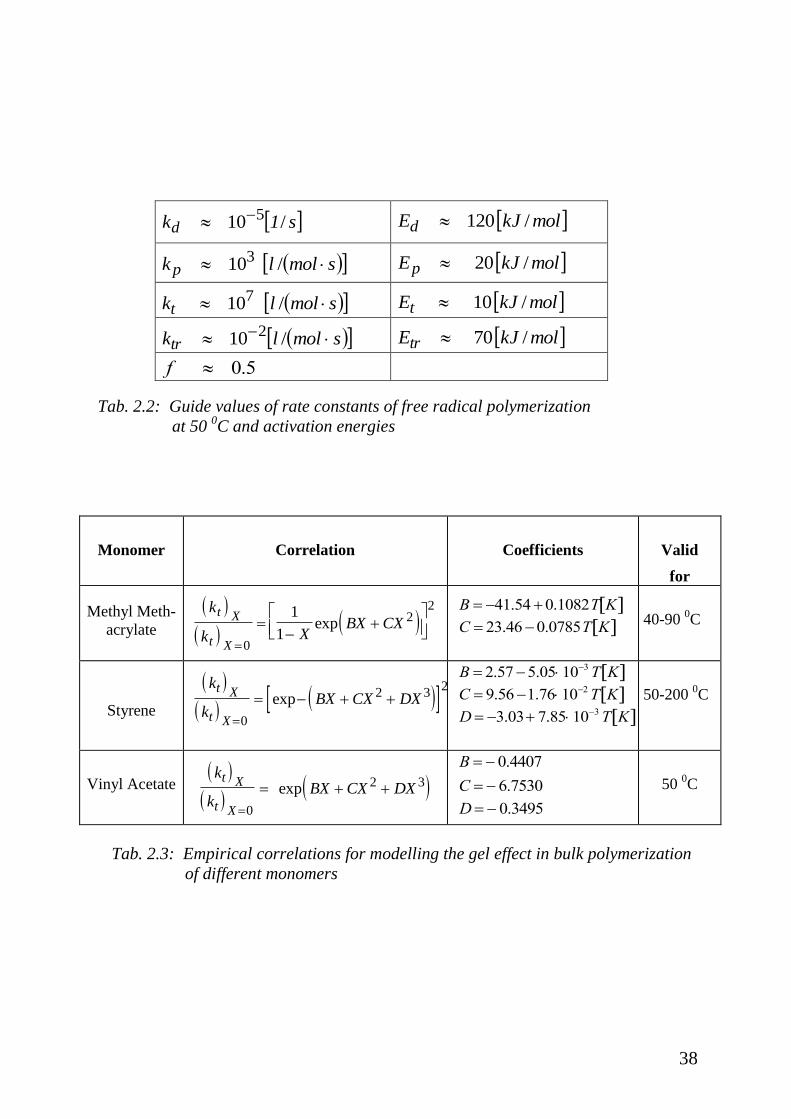
38
s1kd /10 5 molkJEd /120
smollkp /103 molkJEp /20
smollkt /107 molkJEt /10
smollktr /10 2 molkJEtr /70
f 0.5
Tab. 2.2: Guide values of rate constants of free radical polymerization
at 50 0C and activation energies
Monomer Correlation Coefficients Valid
for
Methyl Meth-
acrylate
k
k XBX CX
t X
t X
0
221
1exp
B 41.54 0.1082T K
C 23.46 0.0785T K 40-90 0C
Styrene
k
kBX CX DX
t X
t X
0
2 32
exp
B 2.57 5.05103T K
C 9.56 1.76102T K
D 3.03 7.85103T K
50-200 0C
Vinyl Acetate
k
kBX CX DX
t X
t X
0
2 3exp
B 0.4407
C 6.7530
D 0.3495
50 0C
Tab. 2.3: Empirical correlations for modelling the gel effect in bulk polymerization
of different monomers

39
Monomer Monomer concentration mol/l
polymer particle water
Styrene 5.4 0.005
Butadiene 6.5 0.015
Vinyl chloride 6.0 0.11
Methyl methacrylate 7.0 0.15
Vinyl acetate 7.6 0.3
Tab. 2.4: Monomer concentration in latex particles and water phase at
equilibrium and 500C
Effect on
Increase of
Number
of
particles
Rate
of
polymerization
Molecular
weight
Particle
size
Particle
size
distribution
Concentration
of surfactant increase increase increase decrease broadening
Concentration
of initiator increase increase decrease decrease narrowing
Temperature increase increase decrease decrease narrowing
Volume ratio
of monomer to
water
no effect no effect no effect increase narrowing
no transfer reactions present
Tab. 2.5: Effect of concentration, temperature and phase ratio on different parameters
of emulsion polymerization

40
50 0C E / J mol
-1
ka / lmol-1
·s-1
8.16 10-4 100 000
kp / lmol-1
·s-1
7.83 20 000
kd / s-1
6.46 10-5 25 000
Tab. 2.6 Rate constants for simulation of butadiene gas phase
polymerization without mass transport effect. See Fig. 2.15
50 °C E / J mol-1
0.46 -4000
D / ms-1
3.6 10 –10
17430
ka / lmol-1
·s-1
9 10 –4 100000
kp / lmol-1
·s-1
10 25000
kd / s-1
7 10 –5 20000
ktr cAl / s-1
610-4
Tab. 2.7: Data for simulation of butadiene gas phase polymerization
with mass transport effect. See Fig.2.15
50 °C
0.46
D / ms-1 3.6 10
-10
ka / lmol-1
·s-1 105.5
kp / lmol-1
·s-1
105.5
kd / s-1
7.3110-5
ktr cAl / s-1
610-3
Tab: 2.8: Data for simulation of polydispersion index of gas phase
polybutadiene. See Fig. 2.21

41
ak
1
L
sS ak
1
Mecfk
1
At beginning
of polymerization 20 s 31 s 33 s
After 1 h of
polymerization 20 s 0.1 s 33 s
Tab. 2.9: Different resistances of mass transfer and chemical reaction of
ethylene polymerization in slurry
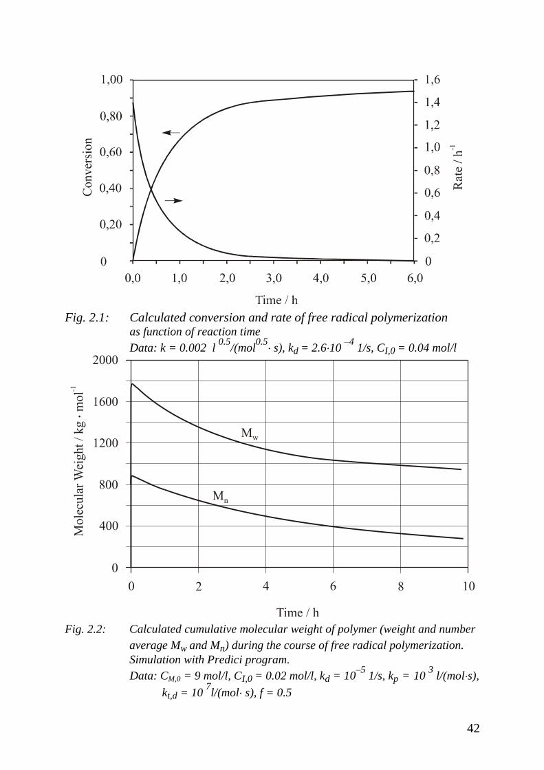
42
Fig. 2.1: Calculated conversion and rate of free radical polymerization as function of reaction time
Data: k = 0.002 l 0.5
/(mol0.5 s), kd = 2.610
–4 1/s, CI,0 = 0.04 mol/l
Fig. 2.2: Calculated cumulative molecular weight of polymer (weight and number
average Mw and Mn) during the course of free radical polymerization.
Simulation with Predici program.
Data: CM,0 = 9 mol/l, CI,0 = 0.02 mol/l, kd = 10–5
1/s, kp = 10 3 l/(mols),
kt,d = 10 7l/(mol s), f = 0.5

43
Fig. 2.3: Effect of monomer concentration (w %) on kinetics of free radical
polymerization of methyl methacrylate at 500C
Fig. 2.4: Rate of styrene polymerization and degree of polymerization at 500C and
different initiator concentrations: a: 0.02, b: 0. 06, c: 0.28 mol/l

44
Fig. 2.5: Decay of termination rate constant with conversion. Bulk polymerization of
a: Vinyl acetate, b: Styrene, c: Methyl methacrylate at 50oC.
Fig. 2.6: Effect of conversion on rate and propagation rate constant of bulk
polymerization of methyl methacrylate at 22.50C (unit of kp in l/(mol s))

45
Fig. 2.7: Correlation of maximum conversion of styrene bulk polymerization and
polymerization temperature
Fig. 2.8: Effect of conversion of methyl methacrylate polymerization in bulk on
radical efficiency factor of initiator

46
Fig. 2.9: Effect of retarder and inhibitor on temporal course of
free radical polymerization
a: no inhibitor or retarder present
b: only retarder present
c: only inhibitor present
Fig. 2.10: Kinetic profile of ideal emulsion polymerization

47
Fig. 2.11: Average number of radicals per particle as function of relative rates of
and m
Fig. 2.12: Monomer concentration CM, number of latex particles N and number of
radicals n during the three periods of emulsion polymerization

48
Fig. 2.13: Initial rate of copolymerization of styrene and methyl methacrylate as
function of mole fraction of styrene in feed.
Dots: experiment. Line: modelling with = 13

49
Fig. 2.14: Particle growth models
Fig.2.15: Rate of gas phase polymerization of butadiene at 500C and 1.6 bar
monomer pressure

50
Fig. 2.16: Equilibrium concentration of 1,3-butadiene in 1,4-cis-polybutadiene
as function of pressure of butadiene and temperature
Fig. 2.17: Molecular weight (number and weight average) of polybutadiene as
function of reaction time. Dots: experiment. Lines: simulation

51
Fig. 2.18: Schematic diagram of concentration profiles of monomer within particle
and gas phase
Fig. 2.19: Diffusion coefficients of butadiene in polybutadiene particles at different
pressure of butadiene and temperature

52
Fig. 2.20: Polydispersion index of molecular weight distribution of polybutadiene.
Simulation with and without effect of mass transport. Polymerization at
1.6 bar and 500C. Simulation data in Tab. 2.6 and 2.7
Fig. 2.21: Polydispersion index of molecular weight distribution of polybutadiene.
Simulation with and without effect of mass transport. Polymerization at
1.6 bar and 500C. Simulation data in Tab. 2.8

53
Fig. 2.22: Kinetic diagram of gas phase polymerization of butadiene simulated with
three different particle models with the same set of kinetic data
Fig. 2.23: Simulated temperature increase of polymerizing particles in gas phase
polymerization of butadiene for two different Nusselt numbers.

54
Fig. 2.24: Concentration profile of monomer in slurry polymerization of ethylene
Fig. 2.25: Effect of catalyst concentration on rate of polymerization. Experimental
results of ethylene polymerization in a bubble column reactor at different temperatures and pressures

55
3. VISCOSITY OF REACTION MIXTURE
3.1 Introduction
During polymerization of monomer the viscosity of the reaction mixture
increases very sharply. This sharp increase in viscosity can have an effect on:
- kinetics of polymerization (gel-, glass-, cage-effect)
- removal of heat from reaction mixture
- generation of heat by stirring of reaction mixture
- degree of mixing of reaction mixture (micro or macro mixing)
- flow pattern of reaction mixture in continuous reactors (residence time
distribution)
Viscosity therefore has a strong influence on reactor performance, reactor
selectivity, and reactor safety. In Fig. 3.1 a schematic of the increase in viscosity
of a reaction mixture of different methods of polymerization is shown. The
strongest increase in viscosity takes place in homogeneous bulk polymerization.
In suspension polymerization, on the other hand, there is almost no increase in
the viscosity of a reaction mixture so long as the volume fraction of the disperse
phase remains constant during the reaction.
3.2 Viscosity of Homogeneous Systems
The viscosity of homogeneous reaction mixtures, either polymer melts or
polymer solutions, is a complex function of many parameters. The following
parameters have an effect on viscosity:
- Molecular weight, molecular weight distribution, chemical and physical
structure of polymer
- Concentration of polymer
- Temperature and pressure
- Shear rate or shear stress
- Type of solvent
In Fig. 3.2 the effect of shear rate on the viscosity of a polymer solution is
shown. The viscosity of the solvent is not dependent on shear rate. The polymer
solution however shows the phenomenon of shear thinning at higher shear rates.
This phenomenon can be explained by disentanglement processes of polymer
molecules at higher shear rates. One very often used correlation to calculate
viscosity of pseudoplastic liquids is that of Ostwald-deWaele. Pseudoplastic
liquids can therefore have different effective viscosities in stirred tank reactors.
At the tip of stirrer the effictive viscosity of pseudoplastic liquids will be much

56
smaller than at the wall of reactor due to different local shear rates. This has to
be considered in the case of heat removal and mixing in stirred tank reactors.
Effect of Molecular Weight of Polymer
In Fig. 3.3 the effect of molecular weight on viscosity of polystyrene-toluene
solutions is shown. The concentration of polymer is 3 wt % and the temperature
is 250C. The region of Newtonian flow behaviour is decreases the higher the
molecular weight of the polymer. At very high molecular weights only non-
Newtonian flow behaviour is observed even at very low shear rates. All lines
end up in a single line with a slope of – 0.83. The slope is a measure for the
degree of pseudoplastic behaviour of the polymer solution. Fig. 3.3 shows that
polymer solutions of the same concentration but different molecular weights can
have the same effective viscosity at a given shear rate. The effect of molecular
weight of polymer on zero shear viscosity can be represented by the following
empirical correlations:
0 = K M
with 2.5 1 for M < Mcr
0 = K´ M3.4
for M > Mcr
K, and K´ depend on polymer/solvent system. The transition from one
correlation to the other occurs in a relative narrow range of molecular weight.
The critical value of molecular weight is obtained by the intersection of straight
lines representing the two regions of the same log-log plot. The transition
behaviour at certain critical molecular weights is attributed to the onset of chain
entanglement of polymer molecules. The critical molecular weight depends on
polymer/solvent systems and varies from 2,000 to 60,000 g/mol.
Effect of Polymer Concentration
The effect of polymer concentration on viscosity can be seen in Fig. 3.4. At
relatively high concentration of polymer no Newtonian regime is present. The
following correlations of zero shear rate viscosity with resprect to concentration
are reported in literature:
0 = PCK with 6.3 3.4 for M > Mcr
0 = PCK with 4.4 ´ 0.5 for M < Mcr
Also in this case there is a critical molecular weight beyond which entanglement
of the polymer molecules will occur and will cause change in flow behavior.
The effect of molecular weight and concentration of polymer on entanglement

57
respectively flow properties can be seen schematically from Fig. 3.5. In practice
the concentration of the reaction mixture is in general larger than 10 weight
percent and the molecular weight is larger than 100,000 g/mol. At these reaction
conditions entangled macromolecules will be present in the reacting system.
Knowledge on the increase of viscosity of a reaction mixture in polymerization
reactors is of interest for the design and control of reactors. One suitable
empirical correlation to calculate the viscosity increase of polymerizing systems
is that of Lyons and Tobolsky. It correlates the zero shear rate viscosity of a
reaction mixture with the viscosity of the solvent, polymer concentration, and
molecular weight of the polymer expressed by intrinsic viscosity []. kH is the
Huggins constant, which does depend on solvent quality. b is an adjustable
parameter.
P
PHPS0
Cb1
C][kexp][C1
η
with
]g/cm[)Xε1(10
MCXC 3
3
MM,0P
/g] [cm MK] [ 3MH
Fig. 3.6 shows an example of the application of Lyons and Tobolsky correlation.
The corresponding parameters of the equation of Lyons and Tobolsky are shown
in Fig. 3.7. Application of the equation of Lyons and Tobolsky on reacting
systems with changing polymer concentration, molecular weight, and average
shear rate should be done with caution.
Effect of Temperature
One widely used empirical correlation to consider the effect of temperature on
the viscosity of liquids is the WLF-equation by William, Landel, and Ferry:
)TT(c
)TT(c)T(ηlog)T(ηlog
ref2
ref1ref
with
c1 17.44 and c2 51.6 if Tref Tg
or
c1 8.86 and c2 101.6 if Tref Tg ~ 43 K

58
This equation holds for a range of temperature from Tg to about Tg +100 K for
many polymers.
3.3 Viscosity of Heterogeneous Systems
The increase in viscosity of a reaction mixture with conversion in suspension
polymerization can be neglected. In case of emulsion polymerization the
increase is moderate. In case of precipitation polymerization the increase can be
significant. This is due to different effects of different parameters on the
viscosity of heterogeneous systems. The viscosity of a dispersion in the liquid
phase depends on following parameters:
- Viscosity of continuous liquid phase
- Volume fraction of disperse phase
- Particle size, particle size distribution, particle shape and surface
properties of particles
- Temperature and pressure
- Shear rate or shear stress
In Fig. 3.8 the effect of shear stress on the viscosity of a polymer latex with an
average particle size of 200 nm is shown for different volume fractions of
disperse phase. From this figure the effect of shear thinning and shear thickening
can be seen, especially in the case of lattices with high solid content. The effect
of shear thinning is attributed to an orientation of latex particles in stream lines.
Shear thickening is attributed to agglomeration effects of latex particles. In Fig.
3.8 another phenomenon can be seen. Concentrated lattices start to flow only if a
certain shear stress is reached.
Effect of Volume Fraction of Particles
One very useful empirical correlation for modelling the viscosity of dispersions
with high solid content is that of Eilers, which is based on the equation of
Einstein.
rel 11.25 P
1 (P / P ,max)
2
This equation was originally derived for narrowly distributed spherical particles
with a maximum volume fraction close to the theoretical value of 0.74. It can be
used, however, also for non-spherical polymer particles like polyethylene
dispersions with much lower maximum volume fractions of solid. Fig. 3.9
shows a plot of relative viscosity of polyethylene suspensions versus volume
fraction of solid. The five polyethylene samples used have different maximum

59
volume fractions from 0.2 to 0.5. The maximum volume fraction of the
polyethylene samples can be determined from the density of the polymer bed
and the density of polyethylene (P,max=bed/PE). Large deviations between
experiment and calculation can be seen only for sample number 5 with the
smallest maximum volume fraction of 0.2. The other 4 samples with maximum
volume fractions of 0.3 to 0.5 can be modeled very well with the equation of
Eilers.
Effect of Particle Size
Experimental studies with dispersions of spherical particles with diameters
larger than 1 m indicate no or only slight effects of particle size on the
viscosity of a suspension. Below 1 m stronger effects are observed. This is
expected since for dispersions of equal solid content, since the distance between
particles will become smaller and the specific interface larger if particles are
getting smaller. The interactions between particles will increase with decreasing
particle size. For dispersions with rough, irregular particles this effect can be
seen even at larger particle diameter. Polydispersity of particle size may also
effect the viscosity of a dispersion. For small particles, effects of surface nature
and electric surface charge are become more pronounced. In this case the
volume fraction must be corrected for the thickness of adsorbed surface layers of
surfactant. If the surfactant is a polymer, the thickness of the surface layer
represents an appreciable fraction of the particle diameter and has to be
considered according to :
3
,
PPeffP
d
2δ1
With being the thickness of the layer of surfactant. In Fig. 3.10 the effect of
effective volume fraction on viscosity of dispersions with different particle size
is shown. In this case a strong effect of particle size on viscosity can be observed
at higher volume fractions. The large variety of dispersions and the large
number of parameters affecting the rheological behaviour of dispersions makes
it difficult to formulate a general correlation for viscosity of dispersions.
3.4 List of Symbols
dP Diameter of particle, m
M Molecular weight of polymer, kg / kmol
(cr: critical, M: monomer, : viscosity average, w: weight average)

60
T Temperature, K
(ref: reference, g: glass transition)
X Conversion of monomer
Shear rate, 1 / s
Thickness of surfactant layer, m
Viscosity, Pas
(o: zero shear rate, s: solvent, rel: relative, []: intrinsic viscosity)
P Volume fraction of polymer
3.5 References
- R.B. Bird, R.C. Armstrong, O.Hassager: “Dynamics of Polymeric
Liquids“, John Wiley and Sons, 1977
- C.W. Macosko: “Rheology, Principles, Measurements and Applications“,
VCH, Publishers, 1994
- H.-U. Moritz: “Increase in Viscosity and its Influence on Polymerization
Process“, Chem.Eng.Technol., 12, 71-87 (1989)

61
3.6 Figures
Fig. 3.1.: Schematic representation of viscosity increase of reaction mixture with
conversion for different methods of polymerization
Fig. 3.2.: Effect of shear rate on viscosity of polymer solution at constant temperature

62
Fig. 3.3: Effect of molecular weight (Mw in g/mol) on viscosity of polystyrene/
toluene solutions
Fig. 3.4: Effect of polymer concentration on viscosity of polystyrene/toluene solutions

63
Fig. 3.5: Molecular weight-concentration diagram of polybutadiene in a good solvent.
Domains of entanglement and no entanglement of polymer molecules
Fig. 3.6: Zero shear rate viscosity of polydimethyl siloxane of different molecular
weight (viscosity average in g/mol)in siloxane solvent at 30oC.
Dots: experiment, lines: simulation
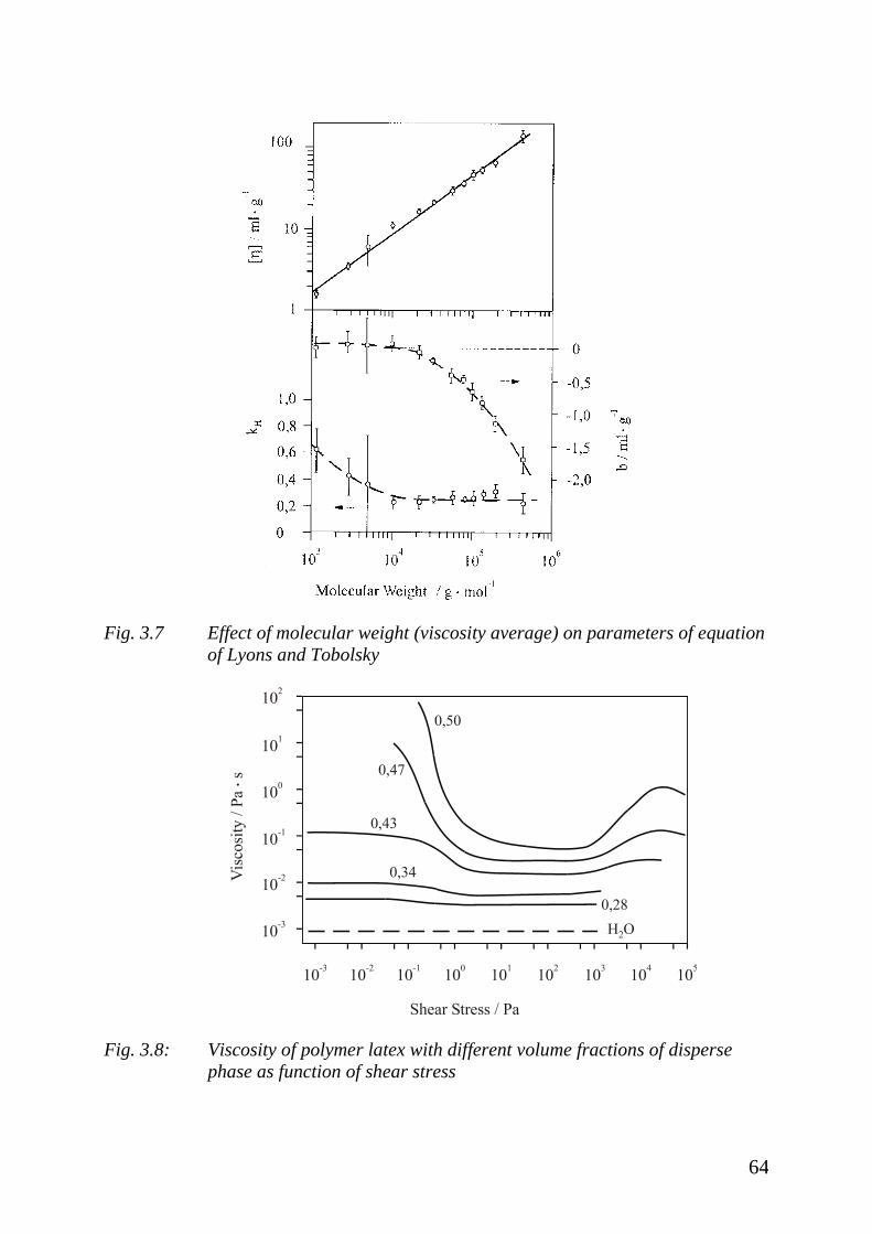
64
Fig. 3.7 Effect of molecular weight (viscosity average) on parameters of equation
of Lyons and Tobolsky
Fig. 3.8: Viscosity of polymer latex with different volume fractions of disperse
phase as function of shear stress

65
Fig. 3.9: Relative zero shear rate viscosity of polyethylene dispersions as function
of volume fraction of polyethylene. Maximum volume fraction of sample
1 to 5: 0.474 / 0.373 / 0.336 /0.339 / 0.195.
Fig. 3.10: Effect of volume fraction and size of particles on viscosity of dispersions
66
4. DATA ACQUISITION OF POLYMERIZATION REACTIONS
4.1 Introduction
For the design of a polymerization reactor, reliable data of polymerization
reactions and polymer properties are necessary. Most important is data on the
kinetics and thermodynamics of the polymerization reaction. But important also
is data on the rheology of the reaction mixture and polymer properties. Very
often this kind of data is not available in literature or is very difficult to find and
not consolidated to one source. In this case data has to be determined by
experimentation. The scale of experimentation depends on data needed. In
general first experiments are run in laboratory scale. The most widely used
technique of polymerization is polymerization in liquid phase. In this case the
most oft used type of reactor is the stirred tank reactor. In laboratory scale
stirred tank reactors with reaction volumes of 1 to 5 liters are used. In Fig. 4.1
the schematic configuration of a stirred tank reactor for data acquisition of
polymerization reactions in liquid phase is given. The unit consists of the reactor
itself, a dynamic thermostat for temperature control, sensors for acquisition of
data, and finally a computer for data mining, modelling and control of the
reactor. Sensors for measuring temperature, pressure, and stirring speed are
available at moderate costs but sensors for measuring viscosity of the reaction
mixture, concentration of reactants or particle size, and molecular weight
distributions of polymer are relatively expensive. A very versatile technique for
on line monitoring of kinetic and caloric data is the method of reaction
calorimetry which has been developed originally in chemical industry for safety
studies.
4.2 Reaction Calorimetry / Kinetic and Caloric Data
Reaction calorimetry is a useful method by which caloric data of chemical
reactions or physical processes can be determined. In the case of polymerization
reactions the rate and conversion can be measured directly if the heat balance of
the system can be solved. Reaction enthalpy and heat transfer coefficient of the
reactor can be determined as well if certain parameters are known. One has to
consider that by reaction calorimetry the total heat production within a reactor is
measured. For exact determination of caloric data one has to know how many
heat producing or heat consuming processes are running in parallel. The parallel
or consecutive processes can be of chemical or physical nature. Therefore the
precise evaluation of caloric experiments is in no way a simple procedure.
Reaction calorimeters can be classified into adiabatic, isoperibolic and
isothermal calorimeters.

67
Adiabatic reaction calorimeter
In this type of calorimeter there is no heat exchange between reaction mixture
and its surrounding. All the heat set free during reaction is accumulated within
the reaction mixture. The temperature of the reaction mixture is increasing with
time and is running into a constant value. In Fig. 4.2 a typical temperature-time
profile is shown. The heat balance is very simple if the temperature increase is
caused by a chemical reaction only. In this case the heat flux by chemistry is
equal to heat flux by accumulation:
accuchem QQ
If only one chemical reaction takes place the temperature of the reaction mixture
is directly proportional to the conversion of this reaction. Adiabatic calorimeters
are relatively simple in construction, they can be used for very fast reactions,
and they are suitable for safety studies. One has to consider that the course of the
reaction may be affected by temperature increase. Side reactions may take place
at elevated temperatures. Effects of temperature and concentration of reactants
on the kinetics of reaction can only be separated by simulation procedures.
Isoperibolic reaction calorimeter
In this case the jacket temperature of calorimeter is kept constant during the run
of reaction. See Fig. 4.3. Part of heat of reaction is transferred to the cooling
agent in the jacket, and the rest is absorbed by the reaction mixture itself. This
can be seen by the temperature increase of the reaction mixture in the beginning
of the reaction. At the end of the reaction temperature of the reaction mixture is
running again into a stationary state. The heat balance of an ideal isoperibolic
reaction calorimeter is given by:
accucondchem QQQ
The heat flux of chemical reaction is equal to the sum of heat flux by conduction
and heat flux by accumulation. Isoperibolic reaction calorimeters are also very
simple calorimeters. They can be run either in an adiabatic way or at sufficient
cooling capacity nearly isothermal. The kinetics of reaction is also affected by
temperature changes. These changes are however relatively small compared to
adiabatic operation procedures. Nevertheless, also in this case the effects of

68
temperature and concentration of reactants on kinetics can only be separated by
simulation procedures.
Isothermal reaction calorimeter
In Fig. 4.4 the temperature profiles of an ideal isothermal reaction calorimeter
are shown. Reaction temperature is constant with time. Jacket temperature is
changing with time depending on the kinetic characteristic of the chemical
reaction. The heat balance is given by:
accucondchem QQQ
One advantage of an isothermal reaction calorimeter is that chemical heat flux is
directly proportional to the rate of chemical reaction. Isothermal reaction
calorimetry is one of the very few methods by which rate of reaction can be
measured on-line during the run of reaction if heat is produced by chemistry
only. Another advantage is that this mode of operation is very often used in
industry. In special cases the heat transfer coefficient of the reactor can also be
determined. On the other hand isothermal reaction calorimeters are extensive
devices, which are rather expensive. Temperatures have to be measured with
high precision. The same is true for measurement of volumetric or gravimetric
fluxes of cooling agent. In practise one has to distinguish between two different
types of isothermal reaction calorimeters. In the case of a so-called heat flux
reaction calorimeter the conductive heat flux through the reactor wall is
determined by measuring the temperatures of reaction mixture T and cooling
agent Tj according to:
)TT(AUQ jcond
For calculation of conductive heat flux condQ the value of UA is necessary. This
value depends on many parameters. One parameter is the viscosity of the
reaction mixture at the wall of the reactor, but also fouling on the wall of the
reactor has a strong input on the heat transfer coefficient U. In the case of
polymerization reactions with a volume contraction of the reaction mixture the
effective cooling area A of reactor will decrease with increasing conversion of
reaction. If using a heat flux reaction calorimeter one has to know the exact
value of UA but also possible changes during the course of reaction. Values of
UA are in general determined by calibration before and after the chemical
reaction. In the case of changes of UA appropriate interpolation operations have
to be done. One way is to correlate UA with the viscosity of the reaction
mixture, which however must be measured during reaction.

69
The other type of isothermal reaction calorimeter is called a heat balance
calorimeter. In this case the convective heat flux of the cooling agent is
measured by measuring the temperatures of the cooling agent at the inlet and
outlet of the jacket of reactor. Furthermore, the gravimetric flux of the cooling
agent also has to be measured with high precision. The convective heat flux is
given by:
)TT(cmQ in,jex,jpconv
The advantage of a heat balance calorimeter is that viscosity, fouling of reactor
walls, and volume contraction will have no impact on caloric measurements.
Both types of reaction calorimeters need the complete heat balance in order to
determine the chemical heat flux necessary for calculation of rate or conversion
of reaction. As an example the heat balance of a heat flow calorimeter shown
schematically in Fig. 4.5 will be discussed. The heat balance reads:
acculoscondchem QQQPQ
chemQ = j
j,Rj )H(RV Heat flux by exothermic chemical reaction
P = Ne N3 d
5 = 2 N MT Heat flux by stirring
condQ = U A (T - Tj ) Heat flux by conduction through reactor wall
losQ = h A (T - Ts ) Heat flux from reactor to surroundings
accuQ = dt
dTCR Heat flux by accumulation
In order to determine chemQ the other four heat fluxes need to be known very
precisely. Problematic is the determination of condQ . It is done by using an
electric heater inside the reactor with a well known heating power elQ . Power
input by stirring and heat loss to surroundings is considered by correction of the
base line of the temperature profile. For the calibration of the calorimeter
determination of the heat transfer coefficient is done by used of the following
equation:

70
)TT()TT(
QUA
jelj
el
The term (T – Tj ) takes into consideration heat loss to surroundings and heat
input by stirring. Calibration is done by measuring first T and Tj without having
the electrical heater in operation, then the heater is turned on and T and Tj are
measured at thermal equilibrium of the reactor. This is done before and after the
chemical reaction. In the case of significant deviations of UA values average
values or interpolations have to be used for calculation of chemQ . With chemQ the
rate and conversion of a reaction can be calculated if only one reaction is taking
place:
Q
dtQ
X)H(V
QR
totalchem,
t
0
chem
R
chem
and
If reaction enthalpy is not known it can be determined by calorimetry according
to:
CX(t)V
dtQ
HM,0
t
0
chem
R
As an example of a polymerization reaction run in an isothermal heat flux
calorimeter, the measured temperature profiles are given in Fig. 4.6. For
calibration of the calorimeter an electrical heat flux of 58 W was introduced into
the reaction mixture for 10 minutes. It can be seen that the temperatures of
jacket are pulled down immediately after turning on the electrical heater and
they go back to original level again after heater is turned off. After 40 minutes
the polymerization reaction is started by injection of the initiator into the reactor.
Again the jacket temperatures are pulled down strongly due to heat production
by polymerization. With decreasing rate of polymerization the temperatures of
jacket are increasing simultaneously. After the end of the polymerization
another calibration was run by introducing again 58 W into reaction mixture.
The response of tempertures is almost the same as that of first calibration. This
is an indication that heat transfer coefficient has not changed during poly-
merization reaction. From this diagram and the heat balance of the calorimeter

71
the rate and conversion of the reaction can be calculated as a function of reaction
time.
4.3 Reaction Viscosimetry/Rheological Data
Viscosity of a reaction mixture is a very important parameter in polymerization
reaction engineering. It can affect reactor performance and safety, but also
product quality. A very useful procedure to measure viscosity of a reaction
mixture in a stirred tank reactor is illustrated in Fig. 4.7. If stirring speed N and
torque of stirrer MT are known the power input of stirrer P can be calculated.
With this parameter the Newton number can be determined. For further
procedure the power input characteristic of the stirred tank reactor must be
known. This characteristic diagram can be measured by mesuring the power
input of the stirrer at different stirring speeds or different viscosities of a
Newtonian liquid and plotting the Newton number versus Reynolds number in a
log-log-plot. A typical power input diagram of a given stirred tank reactor is
shown in Fig. 4.8. From this diagram the corresponding Reynolds number can
be taken if the Newton number is known. With this Reynolds number the
effective viscosity can be calculated. It is evident that this procedure will work
only if the flow pattern of the liquid is within the laminar region. In the turbulent
region the Newton number is constant and viscosity will have no effect on
power input. An important point of this procedure is the precise measurement of
power input. This can be done best by using stirrers with magnetic coupling to
the stirring motor. In this case the friction of the stirrer shaft is minimized.
Reaction viscosimetry was applied to the polymerization of a monomer in
solution using a stirred tank reactor with a helical type of stirrer without baffels.
The corresponding power input diagram is given in Fig.4.8. It was measured by
using sugar solutions of different sugar concentration. Stirring speed was also
changed in order to cover a broad region of Reynolds numbers. From this
diagram and with the data of torque and stirring speed the effective viscosity of
a reaction mixture was determined during the course of polymerization. In Fig.
4.9 the increase of viscosity is shown for three different initial concentrations of
monomer.
4.4 Solubility and Diffusivity of Monomer in Polymer
For modelling of kinetics or molecular weight distribution in multiphase systems
monomer concentration at the local position of active sites has to be known. It is
surprising to see that this kind of data is difficult to find in literature. Very often
experimental studies are the only way of getting information on solubility and
diffusivity of monomers in heterogeneous systems. Solubility and diffusivity of
gases in polymers can be determined by measuring the sorption of gas in
polymer at different pressures and temperatures. These measurements can be
done by using a suitable micro balance. The polymer sample can be used as a

72
film or as a pellet. For determination of correct values of solubility the buoyancy
force has to be taken into account. In Fig. 4.10 the sorption diagram of 1,3-
butadiene in 1,4-cis-polybutadiene is given. Polymer particles of 1.5 mm
diameter were used. Plotted is the solubility of monomer in weight fraction
versus time at 250C and different pressures of butadiene. Equilibrium is reached
between 20 and 40 minutes. Equilibrium concentration of butadiene in
polybutadiene is plotted versus pressure of butadiene at different temperatures in
Fig. 4.11. Dots are experimental results. Lines are calculated by using the
equation of Flory-Huggins:
2MMML,M
M 11lnp
pln
with
T
Eexp0
R
and M
L,M
M
MM
M1c
The equation of Flory-Huggins has to be solved by iteration. The temperature
dependence of Flory-Huggins coefficient can be seen in Fig. 4.12. It can be
described by an equation according to Arrhenius:
T
Eexp0
R
with 0 = 0.105 and E = - 4000 J/mol in case of butadiene/polybutadiene.
There are many ways to determine diffusion coefficient from sorption
measurement. In the present case with spherical polymer particles with narrow
particle size distribution, Fick’s diffusion equation was used as an analytical
solution:
1n2
2P
22
2eq,M
M
n
)r/Dnexp(61
m
)t(m
The result for one experiment is shown in Fig. 4.13. The diffusion coefficients
are, as expected, dependent on temperature, but it was found that they are also
slightly dependent on pressure. This can be seen in Fig. 4.14. The dependence
on temperature can be described according to Arrhenius:

73
T
EexpDD D
0R
with
D0 2.4107 m2 /s and mol/J40017ED in case of butadiene/poly-
butadiene.
Things get more complicated in three phase systems, like for example in the
case of polymerization of propylene in a slurry. Here propylene is first dissolved
in the liquid phase and then in the solid polymeric phase. Hutchinson and Ray
have shown a method for calculation of monomer concentration in the polymer
phase. They were using the theory of Krigbaum-Carpenter. According to this
theory the concentration of propylene in polypropylene is smaller than the
concentration of propylene in solution at partial pressures of propylene between
1 and 10 bars and temperatures between 40 and 70 0C. These results are shown
in Fig. 4.15.
4.5 List of Symbols
A Area, m2
CM Monomer concentration, kmol / m3
cp specific heat capacity, kJ / (kg K)
CR Heat capacity of reaction mixture, kJ / K
D Diffusion coefficient, m2 / s
d Diameter of stirrer, m
E Activation energy, kJ / kmol
HR Enthalpy of reaction, kJ / kmol
h Heat transfer coefficient, kJ / (m2 K s)
MM Molecular weight of monomer, kg / kmol
MT Torque of stirrer, N m
mM Mass of monomer, kg
m Mass flow, kg / s
N Stirring speed, 1 / s
Ne Newton number
P Power input of stirrer, kJ / s
Mp Partial pressure of monomer, bar
L,Mp Vapor pressure of liquid monomer, bar
Q Heat flux, kJ / s

74
R Rate of reaction, kmol / (m3 s)
Re Reynolds number
rP Radius of particle, m
T Temperature, K
U Overall heat transfer coefficient, kJ / (m2 K s)
V Volume of reaction mixture, m3
X Conversion of monomer
Viscosity, Pa s
Density, kg / m3
M Volume fraction of monomer
Flory-Huggins parameter
4.6 References
- J. Brandrup, E.H. Immergut: “Polymer Handbook“, John Wiley and Sons,
1989
- D.W. Van Krevelen: “Properties of Polymers“, Elsevier, 1997
- D.C.H. Chien, A. Penlidis: “On-Line Sensors for Polymerization Reactors“,
JMS-Rev. Macromol. Chem. Phys., C 30 (1), 1-42 (1990), Marcel Dekker
- W. Regenass: “The Development of Stirred Tank Heat Flow Calorimetry as a
Tool for Process Optimization and Process Safety“, Chimia 51 (1997) 189-
200
- F. Rieger, N. Novak: “Power Consumption Scale-up in Agitating Non-
Newtonian Fluids“, Chem. Eng. Sci., 1974, Vol. 29, pp. 2229-2234
- R.A. Hutchinson, W.H. Ray: “Polymerization of Olefins through
Heterogeneous Catalysis. VIII. Monomer Sorption Effects“, J. Appl. Polym.
Sci., 41 (1990), 51
- T.F. McKenna, J. Dupuy, R. Spitz: “Modelling of Transfer Phenomena on
Heterogeneous Ziegler Catalysts. Differences Between Theory and
Experiment in Olefin Polymerization (An Introduction), J. Appl. Polym. Sci.,
57 (1995) 371
- J. Crank, G.S. Park: “Diffusion in Polymers“, Academica Press, 1968

75
4.7 Figures
Fig. 4.1: Configuration of stirred tank reactor for data acqusition of isothermal
batch polymerization in liquid phase
Fig. 4.2: Ideal temperature-time profile of reaction mixture of an adiabatic
calorimeter

76
Fig. 4.3: Ideal temperature-time profile of reaction mixture (T) and jacket
temperature of reactor (Tj) of an isoperibolic calorimeter
Fig. 4.4: Ideal temperature-time profile of reaction mixture (T) and jacket
temperature of reactor (Tj) of an isothermal calorimeter

77
Fig. 4.5: Scheme of heat flow calorimeter for isothermal reaction
Fig. 4.6: Temperature profiles of isothermal reaction calorimeter during period of
calibration and polymerization

78
Fig. 4.7: Procedure for determination of effective viscosity in a stirred tank
reactor by measurement of stirring speed and torque of stirrer

79
Fig. 4.8: Power input diagram of stirred tank reactor with a helical type of stirrer
without baffels
Fig. 4.9: Increase in viscosity of reaction mixture during polymerization in
solution at three different monomer concentrations

80
Fig. 4.10: Absorption diagram of 1,3-butadiene in 1,4-cis-polybutadiene at 250C
and different pressures of butadiene
Fig. 4.11: Equilibrium concentration of 1,3-butadiene in 1,4-cis-polybutadiene as
function of butadiene pressure and temperature. Dots: experiment, lines:
Flory-Huggins equation

81
Fig. 4.12: Flory-Huggins coefficient of the system butadiene/polybutadiene as
function of temperature. Dots: experiment with range of error, line:
Arrhenius equation
Fig. 4.13: Butadiene absorbed in polybutadiene as function of time.
Line: experiment, dots: calculation

82
Fig. 4.14: Diffusion coefficient of butadiene in polybutadiene as function of
pressure and temperature. Dots: fitting to experiment, lines: regression
Fig. 4.15: Equilibrium concentration of propylene in polypropylene as function of
concentration of propylene in n-hexane

83
5. POLYMERIZATION IN STIRRED TANK REACTORS
5.1 Mode of Operation
The most widely used type of reactor in polymer production is the stirred tank
reactor. It is used as single reactor or as a cascade of stirred tank reactors. In the
case of a cascade, three to five rectors are in general connected in series. A
stirred tank reactor can be run batchwise, semi-batchwise, or in a continuous
way. Advantages and disadvantages are listed in Tab. 5.1. Batch reactors are
used in general for small scale production of polymers. It can be used for
production of different types of polymers in short periods of time. A major
disadvantage of a batch reactor is its relatively large cycle time necessary for
filling, heating, cooling, emptying, and cleaning of the reactor as well as for
running of the reaction. Since the reactor is filled at the beginning of reaction
with a large amount of monomer thermal run away phenomena may happen in
the case of failure of cooling. This may lead to thermal explosions of the reactor.
In order to reduce the risk of thermal run away phenomena the semi-batch
operation of a stirred tank reactor can be applied. In this case certain reactants
are not filled into the reactor at the beginning of reaction but they are introduced
into the reactor in a time controlled way. This procedure is applied especially in
the case of production of uniform copolymers when monomers of different
reactivity are used. In this case the less reactive monomer is filled into the
reactor first and the more reactive monomer is pumped into the reactor in such a
way that the ratio of concentration of both monomers is kept constant during the
entire course of copolymerization. Semi-batch operation is also applied in the
case of condensation polymerizations in order to achieve polymers with high
molecular weight. In this case the low molecular weight byproduct of the
condensation reaction is removed permanetly from the reactor in order to shift
the chemical equilibrium reaction to the side of high molecular weight products.
Continuous stirred tank reactors are used for production of large amounts of
polymers with constant quality. In general more than one stirred tank reactor is
used. In a train of stirred tank reactors higher conversions of monomer can be
achieved within a given period of time in comparison to the single continuous
stirred tank reactor. Continuous processes have in general a larger polymer
production performance than batch or semi-batch processes. This is due to the
absence of operation time for filling and emptying of the reactor in case of batch
and semi-batch processes. In general stirred tank reactors are run isothermal but
also non-isothermal operations are known. The volume of stirred tank reactors
can differ very strongly. Reactors with volumes of 100 m3 and more are used in
polymer industry.

84
5.2 Mixing of Reaction Mixture
Types of stirrers and power input characteristic
Mixing of reactants in stirred tank reactors is especially important if reactants
are fed separately into the reactor, or if the polymerization process is run
continuously. In the case of mixing, three characteristic times have to be
considered. Mixing time, time constant of polymerization reaction, and mean
residence time of reaction mixture in case of a continuous process. Mixing time
is the time which is necessary to achieve a certain degree of homogeneity in a
reaction mixture. Time constant of reaction is defined as the ratio of initial
monomer concentration to initial rate of reaction. The mean residence time of an
ideally mixed continuous stirred tank reactor is given by the ratio of reaction
volume to volumetric flow rate of the reaction mixture. For achieving high
reactor performance and selectivity it is logical that mixing time should be much
smaller than characteristic time constant of polymerization reaction and mean
residence time of reactor. In practise mixing time should be at most 10 % of
time constant of reaction or residence time. For good mixing an appropriate
stirrer must be used. Many different types of stirrers are available. They can be
classified according to the resulting flow pattern of the flowing liquid and
according to the viscosity range of liquids which have to be mixed. Some major
types of stirrers used in stirred tank reactors are given in Fig. 5.1. The
corresponding flow pattern indicated by arrows are shown in Fig. 5.2. The task
of mixing can be very different. We have to distinguish between
homogenization of miscible liquids, emulsification of one liquid into another
immsicible liquid, sparging of gas into a liquid phase, or dispersing solid
particles into liquids by stirring. These different mixing tasks will need different
types of stirrers. In Tab. 5.2 a few suitable stirrers for different methods of
polymerization are given. Turbine and propeller agitators are fast running
stirrers used for emulsification of liquids and dispersing of fine solids into
liquids. Blade stirrer is in general used for homogenization of liquids. The
intermig stirrer is a very efficient stirrer used for many tasks but especially for
mixing of disperse systems (gas/solid/liquid). Helical type of stirrers are used for
mixing of highly viscous systems as in case of bulk polymerization of liquid
monomers. For characterization of individual stirrers the power input diagram is
used. The power input characteristic of different stirrers is shown in Fig. 5.3.
The power input of a stirrer is given by:
53dNNeP
It can be measured by measuring the torque of the stirring shaft MT :
TMN2P

85
Knowing P, the Newton number Ne can be determined if stirring speed N,
diameter of stirrer d, and density of liquid phase is known. This dimensionless
Newton number is plotted in a logarithmic diagram versus dimensionless
Reynolds number of stirrer. From this power input diagram different flow
regions can be characterized.
Laminar region (Ne Re = constant):
32 dNCP
with 1ReatNeC
Turbulent region (Ne = constant) :
53 dNNeP
From the power input diagram the following information can be taken:
- Determination of power input in a given liquid for a given stirrer at given
stirring conditions. First the Reynolds number is calculated than the Newton
number is taken from the diagram. With this Newton number the power
input is calculated.
- Comparison of different stirrers with respect to power input at given
Reynolds number.
- The effect of baffles on power input at given Reynolds number.
In the case of non-Newtonian homogeneous liquids like polymer solutions the
power input characteristic is similar to Newtonian liquids if Reynolds number is
determined by using the effective viscosity of liquid phase (Reeff = N d2 / eff).
The effective viscosity of the non-Newtonian liquid at a given stirring speed can
be determined by measuring first the viscosity as a function of shear rate in a
rotational viscosimeter. Then the correlation between shear rate and rotation
frequency of the stirrer is necessary. For this purpose correlations of Metzner
and Otto can be taken which are only valid for laminar region. Correlations of
Metzner and Otto have the form NK with K = 10 for propeller, K = 12
for turbine and K = 30 for helical ribbon agitator.
For gas/liquid or gas/solid/liquid dispersions one has to take into account that
the Newton number is a function of gas throughput. It decreases with increasing
flow rate of gas.

86
Mixing of miscible liquids
Homogenization of miscible liquids is one of the most often used unit operations
in chemical engineering. The homogenization process of liquids in stirred tank
reactors can be regarded as a two step process. In the first step mixing will take
place by convection of the liquid phase. In the case of turbulent mixing small
volume elements of liquid will be formed. The smallest volume elements which
will be formed can be expressed by the theory of Kolmogorov. The micro scale
of turbulence [m] depends on the specific energy input of stirring [W/kg or
m2/s
3] and on the viscosity of the liquid [m
2/s] and is given by:
4/1
3
In the case of water with a viscosity of 10-6
m2/s and an energy input of 1 W/kg,
the diameter of segregated volume elements is 32 m. In the case of glycerine
with a viscosity of 10-3
m2/s and the same energy input the scale of volume
elements is already 5.6 mm. This shows that viscous liquids like polymerization
mixtures are always to some extent segregated systems. Power input of stirring
has only a small effect on micro scale of turbulence ( -0.25). In the second
step of turbulent mixing the interior of the micro scale volume elements is
mixed by diffusion. This kind of mixing is called micro mixing and takes place
on a molecular scale. The mixing time by diffusion is given by:
D
2
With the diffusion coefficient on the order of D = 10 –9
m2/s, which is typical
for liquids, the micro mixing time is 1 second for water and 30 seconds for
glycerine. This result shows, that micro mixing is fast compared to macro
mixing by convection. Macro mixing does depend on the scale of the reactor.
Micro mixing is scale independent.
Mixing times of liquids in reactors are in general determined by experiment
since many parameters may affect the numerical values. In practise, physical
and chemical methods are applied. A mixing time has to be connected with a
degree of mixing. In Fig. 5.4 the mixing characteristics of different types of
stirrers with and without baffles are given. Mixing time refers to perfect
mixing (micro mixing). For mixing of highly viscous liquids the helical ribbon
stirrer is an effective type of stirrer. It is used for mixing in the laminar flow
regime. Mixing time is affected by stirring speed. In case of blade stirrers one
can classify two regimes of mixing:

87
1. Re = 10 to 10 2 : N 1/Re : / (Nd)
2
2. Re 10 3
: N const : 1 / N
In the laminar regime time of mixing does depend on viscosity and strongly on
stirring speed and the diameter of the stirrer. In the turbulent regime time of
mixing is independent on viscosity and the scale of the stirrer. It is affected only
by stirring speed.
In polymerization reactors very often liquids with differences in density and
viscosity have to be mixed. Furthermore, a reaction mixture may have non-
Newtonian flow properties. In this case mixing characteristic becomes more
complex and mixing number N is not only dependent on the Reynolds number
but also on the Archimedes number, which is defined as:
2
3 gdAr
Mixing time will depend on average density and viscosity but also on gravity
and the density difference of the two liquids. Non-Newtonian mixtures are
homogenized much slower than Newtonian liquids at same mixing conditions in
the laminar and transient regimes of flow. This is due to the fact that there is a
shear rate gradient in the reactor which causes large viscosity differences. The
viscosity of reaction mixture is increasing from stirrer to reactor wall.
Opara studied the mixing behavior of non-Newtonian liquids in stirred tanks in
transient regimes of flow and noticed the formation of non-mixed zones in the
form of vortex rings which rotate around the stirrer. Mixing within these rings is
slow compared to mixing in the well mixed part of reactor. In this case two
different mixing times have to be considered. Mixing by convection is fast
whereas mixing by diffusion in the stagnant rings is a slow process. Total
mixing time of non-Newtonian liquids can be about 10 times larger than for
Newtonian liquids if mixing is done in the laminar regime. In turbulent regimes
the differences become less and less.
Mixing of non-miscible liquids
In emulsion and suspension polymerization liquid monomers are dispersed by
stirring into the surfactant-containing water phase. In suspension polymerization
water soluble polymers are used as surfactants. The average particle size of
monomer droplets in this case is determined by parameters like:
- Physical properties of the two liquids (viscosity, interfacial tension, density)

88
- Geometry of the stirred tank (type, number and position of stirrer and baffle,
ratio of hight to diameter of reactor, ratio of stirrer diameter to reactor
diameter
- Operation conditions (stirring speed, time of stirring and polymerization,
volume ratio of phases, degree of filling of reactor, temperature, batchwise
or continuous operation)
In the case of turbulent mixing the following type of equation is proposed in
literature for calculation of the mean diameter of monomer droplets:
M25/3
132 C1WeCd
d
with
i
2ii
i
3ii
32dn
dn
d
C23 Nd
We (Weber number)
The constants C1 and C2 depend on the chemical and physical system used. This
correlation must be used with caution since at larger Weber numbers deviations
are reported in literature.
If the factor M2C1 is neglected, the following correlation between droplet
diameter and power input by stirring is obtained:
4,0
332 Cd
with V
P
C
These kind of correlations have also been reported for average diameter of
polymer particles produced in suspension polymerization at high concentration
of surfactants. The constant C3 is determined mainly by the physical properties
of the two phase system and by the energy distribution of stirring within the
reactor volume.
(Sauter mean diameter of
monomer droplets)

89
In the case of vinyl chloride polymerization in suspension, the effect of Weber
number (i.e stirring speed) on the average diameter of polymer particles is
shown in Fig. 5.5. It can be seen that at Weber numbers larger than 3105 the
particle size is no longer decreasing with increasing Weber number, but
becomes independent of Weber number and at very large Weber numbers it is
even increasing. The three zones of Weber numbers are explained by different
interaction between processes of particle break-up, particle coalescence, and re-
agglomeration of particles.
Mixing of gas in liquid phase
In slurry polymerization of ethylene or propylene in stirred tank reactors the gas
phase is dispersed into an organic liquid (low boiling hydrocarbon). The rate of
mass transfer of monomer from gas to liquid phase is given by:
ML CakR
with V
Aa (specific interface)
L,MMM CCC (see Fig. 2.24)
k L = D/
The saturation concentration of monomer in liquid phase MC does depend on
the kind of monomer and liquid, partial pressure of the monomer and
temperature. The concentration of monomer in liquid phase CM,L depends on the
rate of mass transport and rate of polymerization.
The liquid-side mass transfer coefficient kL is defined according to “two film“-
theory as the ratio of diffusion coefficient of transfer component D to thickness
of liquid-side boundry layer . Effective sparging of liquid phase with gas can
be done with a turbine agitator. The gas phase is introduced into liquid phase
through a pipe placed below the stirrer. The kLa value is affected by gas flow
rate. Gas flow rate may affect also power input of stirring. With increasing gas
flow rate the relative gas hold up of liquid phase is increasing and density of
disperse system is decreasing. This will lead to a decay in power input by
stirring. In Fig. 5.6 the decay in Newton number with increasing gas flow rate is
shown in the case of a 6 blade turbine stirrer with gas inlet below the stirrer. The
gas flow rate is expressed by a dimensionless gas flow number Q. This
correlation is valid within certain limitations. At larger gas flow numbers the gas
dispersing efficiency of stirrer will be lost completely because beyond certain
flow rates the stirrer will be surrounded completely by gas phase. The numerical
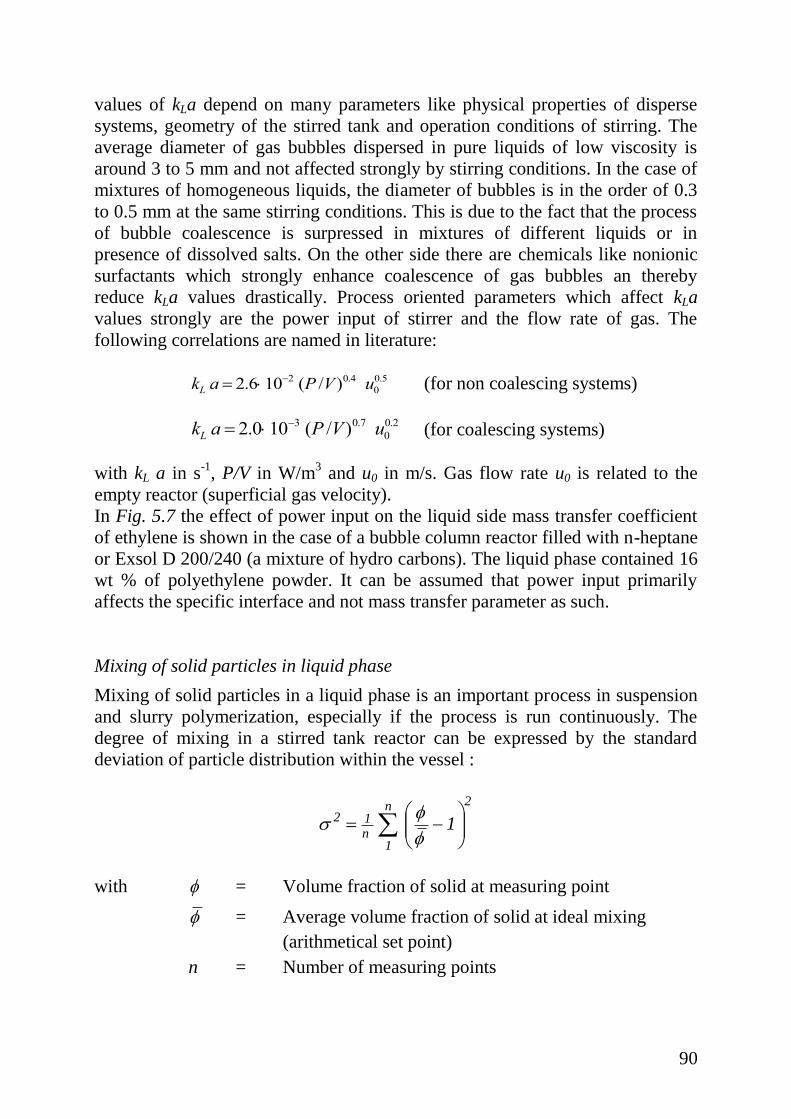
90
values of kLa depend on many parameters like physical properties of disperse
systems, geometry of the stirred tank and operation conditions of stirring. The
average diameter of gas bubbles dispersed in pure liquids of low viscosity is
around 3 to 5 mm and not affected strongly by stirring conditions. In the case of
mixtures of homogeneous liquids, the diameter of bubbles is in the order of 0.3
to 0.5 mm at the same stirring conditions. This is due to the fact that the process
of bubble coalescence is surpressed in mixtures of different liquids or in
presence of dissolved salts. On the other side there are chemicals like nonionic
surfactants which strongly enhance coalescence of gas bubbles an thereby
reduce kLa values drastically. Process oriented parameters which affect kLa
values strongly are the power input of stirrer and the flow rate of gas. The
following correlations are named in literature:
kL a 2.6102 (P /V )0.4 u0
0.5 (for non coalescing systems)
kL a 2.0103 (P /V )0.7 u0
0.2 (for coalescing systems)
with kL a in s-1
, P/V in W/m3 and u0 in m/s. Gas flow rate u0 is related to the
empty reactor (superficial gas velocity).
In Fig. 5.7 the effect of power input on the liquid side mass transfer coefficient
of ethylene is shown in the case of a bubble column reactor filled with n-heptane
or Exsol D 200/240 (a mixture of hydro carbons). The liquid phase contained 16
wt % of polyethylene powder. It can be assumed that power input primarily
affects the specific interface and not mass transfer parameter as such.
Mixing of solid particles in liquid phase
Mixing of solid particles in a liquid phase is an important process in suspension
and slurry polymerization, especially if the process is run continuously. The
degree of mixing in a stirred tank reactor can be expressed by the standard
deviation of particle distribution within the vessel :
2n
1n
12 1
with = Volume fraction of solid at measuring point
= Average volume fraction of solid at ideal mixing
(arithmetical set point)
n = Number of measuring points

91
In Fig. 5.8 the distribution of glass beads within a stirred tank reactor at different
stirring speeds is shown. The reactor has a diameter of 365 mm. The diameter
ratio of propeller stirrer to reactor is 0.315. The position of the stirrer within the
reactor is marked with hS. The glass beads have a diameter of 200 m. The
volume fraction of glass beads is 0.1. Water was used as liquid with a viscosity
of 10-3
kg/ (ms). The relative density difference of the dispersion is 1.87. As can
be seen from Fig. 5.8, the homogeneity of the suspension is improves with
increasing stirring speed. A perfectly mixed suspension would have a relative
solid content of 1 and a standard deviation of 0 at any position within the reactor
volume. At a standard deviation of 0.25 the glass particles are totally distributed
within the reactor volume, although not evenly. In practise this standard
deviation is the upper limit from an energetic and mechanical stand point. In the
case of slurry polymerization of olefins the relative density difference of the two
phases is smaller and a distribution of solid particles within the total reactor
volume may be reached at higher standard deviations ( 0.5).
The effectiveness of stirrers for mixing of solid particles into liquids can be
quite different. In Fig. 5.9 the standard deviation of mixing versus power input
of the stirrer is plotted for different stirrers at the same mixing conditions. As
can be seen, the so called intermig stirrer has the best mixing effectiveness at the
lowest power input.
The rate of mass transfer of monomer from liquid to solid phase is given by:
MS CakR
with V
Aa (specific interface)
S,ML,MM CCC (See Fig. 2.24)
The mass transfer coefficient kS for a single sphere of diameter dP at rest within a
large volume of stagnant fluid is given by kS = 2 D/dP. D is the diffusion
coefficient of monomer in the liquid phase. Any motion of the spherical particle
relative to the liquid phase will increase the numerical value of kS. The following
dimensionless correlation is proposed for mass transfer of flow past single
spherical particles covering the entire range of hydrodynamics with respect to
the Reynolds number.
3/12/1 ScRe76,00,2Sh
with D/dkSh PS

92
/duRe P
D/Sc
In slurries of small particles in a gently stirred liquid the relative velocity of the
two phases is low and roughly that of free fall of a particle due to gravity. The
terminal velocity of small spheres in a stagnant liquid is given by the law of
Stokes:
18
dgu
2P
Using the Sherwood equation and Stoke’s law, kS as a function of dp can be
calculated. The correlations are plotted in Fig. 5.10 for suspensions of different
density differences. Slurries of catalyst particles suspended in a liquid are
agitated vigorously to keep the particles well dispersed and to promote
absorption of the monomer gas. The resulting turbulence in the slurry phase
promotes mass transfer and the actual mass transfer coefficient will be larger
than that taken from Fig. 5.10. As a first approximation the actual mass transfer
coefficient may be twice the value taken from Fig. 5.10 based on Sherwood
numbers with termal velocity of particle in free fall.
One of the best ways of estimating kS is correlations for mass transfer in agitated
slurries based on power input of stirrer, provided that power input is wellknown.
Calderbank and Moo Young for example have published the following equation:
4/13/2
S )(13,0Sck
with V
dNNe 53
The exponent of the Schmidt number has to be taken with caution since other
lower values have also been published.
5.3 Heat Removal and Safety Aspects
Heat removal and heat formation
Heat can be removed from stirred tank reactor in different ways. See Fig. 5.11.
The following methods of heat removal are used:
- Indirect cooling by jacket of reactor, by internal cooling coils or by external
heat exchanger
- Direct cooling by feed of reaction mixture or by evaporation of monomer or
solvent

93
A common problem of heat removal from polymerization reactors is the
tendency of reaction mixtures to form polymer films on the wall of cooling
areas.
These films can reduce the heat exchange capacity of heat exchangers very
strongly. If external heat exchangers are applied then the reaction mixture has to
be pumped through the heat exchanger and this may cause strong pressure
drops, especially if the reaction mixture is highly viscous. In the case of heat
removal by evaporation of a liquid phase inside the reactor, the formation of
foam may happen. The foam may rise into an external heat exchanger and block
the piping. Remixing of a condensed liquid with viscous reactor content may
also be difficult. Indirect cooling takes place by conduction of heat through the
walls of heat exchangers whereas direct cooling happens by convection of heat
by flowing liquids or vapors.
Heat formation inside a polymerization reactor can happen by chemical reaction,
by stirring or by physical processes like in-situ crystallization. Polymerization
reactions are in general exothermic reactions with very different reaction
enthalpies. Heat formation by stirring has to be considered when highly viscous
liquids are stirred.
The heat balance of a continuous stirred tank reactor can be expressed by the
following equation:
evapconvcondchemaccu QQQPQQ
with dt
dTcmQ paccu (heat flow by accumulation)
VHRQ Rchem (heat flow by chemical reaction)
53dNNe P (heat flow by stirring)
Jcond TTAUQ (heat flow by conduction)
0pconv TTcmQ (heat flow by convection)
evapevap HnQ (heat flow by evaporation)
The previous heat balance does not consider heat losses of the reactor to
surroundings nor heat formation by physical processes like crystallization of
polymer formed.

94
In the case of heat flow by accumulation one has to keep in mind that heat is not
only absorbed or generated by the reaction mixture but also by the reactor itself.
Heat formation by polymerization reaction does depend on the rate of monomer
polymerization. This rate can be constant with time as in the case of continuous
processes at stationary state, or it can change with time as in the case of batch
processes. In general it will fall with increasing conversion of monomer. In auto-
catalytic polymerization reactions it will first increase with time and then
decrease during the course of reaction. Monomers like styrene, butadiene, vinyl
chloride, propylene, and ethylene have reaction enthalpies in the range of -70 to
-100 kJ/mol. Condensation polymerization reactions have much lower reaction
enthalpies. The reaction enthalpy of poly(ethylene terephtalate) synthesis is
about -10 kJ/mol. Addition polymerization reactions like polyurethane synthesis
are strongly exothermic reactions with enthalpies of about -200 kJ/mol. The
catalytic synthesis of resins like phenol/formaldehyde and urea/formaldehyde
are also very exothermic reactions.
Heat formation by stirring has to be considered, especially if highly viscous
reaction mixtures are to be mixed by stirring. Viscous liquids are mixed in
laminar regimes of flow. Here the Newton number is inversely proportional to
the Reynolds number and power input by stirring is proportional to viscosity of
liquid and proportional to the second order of stirring speed.
Most important in heat removal of polymerization reactors is heat transport by
conduction. The heat transfer coefficient U is affected by the geometry of the
reactor, by physical properties of reaction mixture (viscosity, thermal
conductivity, specific heat capacity), and by operation conditions of mixing
(stirring speed, temperature). The heat transfer coefficient of a stirred tank
reactor with clean walls can be expressed according to Peclet as:
jw
w
r h
1d
h
1
U
1
The total resistance of heat transfer is given by the addition of three single
resistances, namely the resistance of heat transfer from reaction mixture to
reactor wall, the resistance of heat transfer through the wall of reactor with
thickness dw and thermal heat conductivity w, and finally the resistance of heat
transfer from reactor wall to cooling agent within the jacket of the reactor. The
single heat transfer coefficients hr and hj are given by the ratio of thermal heat
conductivity of the corresponding liquid and the thickness of boundry layer of
liquid. The thermal heat conductivity of steel is in the range of 15 to
20, of polymer 0.2 to 0.3, of organic liquids 0.1 and of water 0.6 W/(mK). The

95
thickness of the boundary layer does depend on physical properties of the liquid
phase and stirring conditions. In general the main resistance of heat transfer is
the resistance of heat transfer from the reaction mixture to the reactor wall if the
wall is not covered by a thick film of polymer. In this case so called Nusselt
correlations can be used to determine the numerical values of hr and
subsequently U. For homogeneous Newtonian liquids the following Nusselt
equation can be used for turbulent region of mixing (Re>200) :
Nu const. Re2/3 Pr1/ 3 Vis0.14
with
rr DhNu ;
2dNRe
pcPr ;
)T(
)T(Vis
j
The constant of heat transfer characteristic has numerical values from 0.3 to 0.8
for fast rotating agitators and up to 10 for slowly rotating agitators. The
exponent of the viscosity number depends on heat flow direction. For cooling it
is smaller than 1 and for heating it is larger than 1.
In the laminar regime of flow the effect of Reynolds number on heat transfer
becomes less. For a helical ribbon agitator the following correlation is given:
Nu 4.2 (Re Pr)1/ 3 Vis0.2
This correlation should be valid for Newtonian and non Newtonian liquids as
well, if effective viscosities are used.
It has to be remembered, however, that the heat transfer coefficient of a
polymerization reactor can change strongly during the course of a
polymerization reaction. In Fig. 5.12 the change of heat transfer coefficient of a
2 liter steel reactor with helical ribbon agitator at 160 rotation per minute is
shown for solution polymerization of methyl methacrylate with an initial
concentration of 55 weight percent. The decrease of heat transfer coefficient
with increasing conversion of monomer is caused by the increase of viscosity of
reaction mixture.
The previous correlations of heat transfer are valid for homogeneous reaction
mixtures. In the case of heterogeneous reaction mixtures the same correlations
can be used if average values of physical properties of dispersions are taken into
account. If the reaction mixture is a sparged liquid than additional parameters
like superficial gas velocity and gravity have to be considered. The heat transfer
correlation has, in this case, a different form:

96
a2 )FrPr(ReconstSt
with 0p
r
uc
hSt
;
duRe 0 ;
pcPr ;
gd
uFr 0
Heat removal by convection can only be applied in the case of continuous or
semi-batch reactors. The heat flow by convection is mainly determined by mass
flow of feed and by the difference of temperatures between inlet and outlet. The
specific heat capacities of organic liquids are about 2 kJ/(kgK). Water has a
heat capacity of about 4 kJ/(kgK). One industrial example of direct cooling by
feed of reaction mixture is the process of free radical ethylene polymerization at
high pressure and temperature. Due to reactors with thick walls only a small
amount of heat can be removed by indirect cooling via the jacket. The rest of the
heat is removed by direct cooling via convection. Another example is the gas
phase polymerization in fluidized bed reactors with heat removal mainly by
convection.
Heat removal by evaporation is used if polymerization can be run at the boiling
temperature of the monomer or solvent at the conditions given. The heat flow by
evaporation is given by the molar flow of monomer or solvent and by the
enthalpy of evaporation. The molar flow is controlled by the area of evaporation.
The heat of evaporation depends on the type of monomer or solvent. The
numerical values are in the range of 15 to 40 kJ/mol. Cooling by evaporation is
used in production of resins of phenol and formaldehyde in water as solvent.
The reaction temperature is kept constant at 95oC by this method of cooling.
The cooling capacity of a stirred tank reactor is defined as the difference
between heat removal by conduction and heat production by stirring. The
difference should be as large as possible. The maximum value of cooling
capacity is connected to an optimum value of rotation of the agitator. This can
be seen in Fig. 5.13, which shows the effect of stirring speed on the cooling
capacity of the reactor. The dotted lines in Fig. 5.13 show the effect of stirring
speed on heat removal by conduction and on heat production by stirring. In the
laminar regime of flow heat generation by stirring is proportional to the second
power of stirring speed, whereas heat removal by cooling via jacket is only
proportional to the square root of stirring speed. That is why the cooling
capacity of a reactor runs through a flat maximum of about 30 kW in the case of
Fig. 5.13, and the optimum rotation number of the stirrer is about 20 rotations
per minute. Very often stirring speed will not be fixed by cooling capacity of
reactor but rather by the degree of mixing of the reaction mixture. The quality of
mixing is in general more important since it can affect polymer quality to a great
extent.

97
Thermal stability of the continuous stirred tank reactor
Safe operation of a reactor means that it should not burst or leak. Bursting of a
reactor can be caused by uncontrolled temperature increase beyond certain
limits. In order to understand how fast the temperature of a reactor will increase
and to what upper level it will rise in the case of a disturbance in cooling,
simulation studies of thermal stability of the reactor should be done. P. Wittner
and others have studied thermal runaway phenomena in the thermal
polymerization of styrene in bulk phase in a continuous stirred tank reactor. First
order reaction kinetics were used for modelling the polymerization reaction. The
following heat and mass balance was used:
T
0T
pjR0p
Tdc1
)TT(q)H()X1(knc
1
td
Td
with Tcc 0,pp ;
TR
Eexpkk 0
V
AUq ;
m
V
n0 : Feed concentration of monomer [mol/kg]
X)X1(k
td
Xd
At stationary state: )X1(k
X
st
st
Data used for simulation:
k0 = 1,4109
1/min cp,0 = 0,4 kJ/(kgK)
E = 89 kJ/mol = 4.310-3
kJ/(kgK)
(- HR) = 74 kJ/mol T0 = 288 K
q = 12.310-3
kJ/(kgKmin) jT = 358 K

98
Results of simulation:
In Fig. 5.14 the rate of heat generation and heat removal is plotted versus
temperature of reaction at a constant mean residence time of 388 minutes. Heat
generation is a complex exponential function and heat removal is a linear
equation. The two curves cross each other in three points which represent
potential operating points of reactor. The lowest crossing point represents
virtually no reaction. The polymerization reaction has not initiated. Whereas
crossing points P1 and P2 are realistic operating point with high conversion of
monomer at conditions given. Inspection of these two points P1 and P2 reveals
that P1 is a non stable operating point whereas P2 is a thermally stable point. At
point P1 a small rise in temperature would produce a greater generation of heat
than removal. Hence temperature would tend to increase further until operating
point P2 is reached. Similarly, a drop in temperature would induce a greater drop
in temperature and temperature will fall till the lowest operating point is
reached. This phenomena does not apply to operating point P2 which is
thermally stable. Fig. 5.14 does not reveal how fast these transitions from one
operating point to the other will take place. In this case the transition
characteristic of the process has to be simulated by simultaneous solution of
both differential equations. In Fig. 5.15 the transition of operating point P1 (at
130 0C and 60% conversion) to operating point P2 (at 170
0C and 95 %
conversion) is shown, when cooling temperature of the jacket increases by two
degrees. It takes about 600 minutes until the new operating point is reached. One
of the worst cases is the total break-down of cooling and feeding of the reactor.
This causes an adiabatic runaway of reactor temperature. The result of a
simulation is shown in Fig. 5.16. Temperature is rising within 50 minutes to a
maximum value of nearly 260 0C. The adiabatic temperature increase is given
by:
p
RO,Mad
c
)H(CT
5.4 Residence Time Distribution
If molecules or elements of a fluid are taking different routes through the volume of a continuous operated reactor, they will spend different times within such a reactor. The distribution of these holding times is called the residence time distribution (RTD) of the fluid. The RTD can affect the performance of a reactor and may also have a strong input on the selectivity of a chemical reaction. In the case of polymerization reactions the RTD can have an effect on the molecular weight distribution of the

99
polymer formed. This will mainly be the case when the mean life time of the active species of the polymerization reaction is in the same order of magnitude like the mean residence time of the reactor. In this case polymers with a narrow molecular weight distribution can only be produced in a reactor with narrow RTD. The RTD in the case of polymerization reactions can also play a major role if the reaction mixture is a segregated system. Segregation in the reaction mixture can easily occur if the reaction mixture is of high viscosity or a heterogeneous nature, with elements that act as individual micro reactors without an exchange of mass. The RTD of a polymerization reactor is therefore an important parameter which may affect the performance of the reactor and also the properties of the polymer formed.
Experimental methods for determination of RTD
Most important for determination of the RTD of a reactor is the application of a suitable tracer. A suitable tracer should be easy to detect and the total amount of injected tracer should be detectable at the exit of reactor. The most important methods for the determination of the RTD are the so called pulse and step experiments. They are easy to perform and interpret.
a) The pulse experiments
In this case a certain amount of a tracer is added pulse-wise to the fluid entering the reactor and the concentration-time relation of the tracer at the exit of reactor is recorded. This is shown schematically in Fig. 5.17. From the balance of material for the reactor the mean time of the concentration-time distribution can be found.
Mean time (holding time):
iii
iiii
0
0
tC
tCt
Cdt
tCdt
t
[s]
To find the RTD, which is also called the exit age distribution E, concentration-time distribution has to be normalized in such a way that the area under the distribution curve is unity. For doing this the concentration readings have to be divided by the area under the concentration curve. This is shown in Fig. 5.18. The relationship between C and E curves only holds exactly for reactors with so called closed boundary conditions. This means that the fluid only enters and only leaves the reactor one time. No adsorption of tracer at the walls of the reactor should happen. Very often it is convenient to use a dimensionless Eθ curve for reasons of comparison of reactors. In this case time is measured in terms of mean residence time t/t . Then EtE .

100
b) The step experiment
In this case the tracer is not introduced pulse wise into the fluid entering the
reactor but is introduced in a continuous way by injecting a constant side stream
of tracer to the fluid entering the reactor and measuring the outlet tracer
concentration C versus time as shown in Fig. 5.19. The mean residence time is
given by following equation:
max
max
max
C
0max
C
0
C
0 tdCC
1
dC
tdC
t
The dimensionless form of the concentration curve is called the F curve or
transition function. Here the tracer concentration is rising from zero to unity
with time (see Fig. 5.20).
RTD of mixed flow reactors with ideal flow pattern
Fig. 5.21 shows the residence time distribution of a cascade of N equal size well
mixed stirred tank reactors which are connected to each other in series. The most
narrow distribution is shown by the cascade of stirred tank reactors with an
infinite number of vessels. The broadest RTD results in case of a single stirred
tank reactor. The RTD of equal sized stirred tank reactors with mixed flow is
given by the following equations:
t
NtN1N
e!1N
N
t
t
t
1E
with itNt (N : number of reactors and ti : mean time of single reactor)
1N2
t
Nt
t
Nt
)!1N
1...
t
Nt
!2
1
t
Nt1e1F
RTD of mixed flow reactors with non-ideal flow pattern
In reality the flow pattern of reactors deviate from ideal mixed flow pattern. This
is especially the case for polymerization reactors in which a polymer solution or
dispersion with high viscosity is flowing through the volume of the reactor,
causing a non-ideal flow pattern. Non-ideal flow patterns can result for example

101
if the reactor volume contains so called dead or stagnant regions or if bypass or
recycle flow is present next to the active flow through reactor regions of mixed
flow. If these non-ideal flow patterns are present in a given reactor they can be
seen easily by looking at the corresponding experimental RTD. The following
models can be used to describe the measured RTD of real reactors with
deviation from ideal flow:
Compartment Model
Dispersion Model
Tanks-In-Series Model
Convection Model (for laminar flow in pipes)
In Fig. 5.22 compartment flow models are given for a stirred tank reactor which
is characterized by the presence of dead zones and bypass. The corresponding
RTD of the two compartment models are shown in Fig. 5.23. The dispersion and
tanks-in-series model is used in general when small deviations from plug flow
are expected. They are one parameter models. A dispersion number is used in
the case of the dispersion model whereas the number of stirred tanks is used in
case of the tanks-in-series model.
The convection model is used if a viscous liquid is pumped through a tubular
reactor. In general the flow is of a laminar characteristic with a parabolic
velocity profile. Thus the spread in residence times is caused only by velocity
variations. The velocity profile of a laminar flow is shown together with the
corresponding RTD in Fig. 5.24.
5.5 Reactor Performance
Conversion, reaction volume and reactor capacity
Reactor performance of a given stirred tank reactor depends on the mode of
operation. In Tab. 5.3 correlations of conversion and reaction volume are given
for different types of stirred tank reactors (batch reactor, homogeneous
continuous stirred tank reactor, cascade of equal sized stirred tank reactors). The
correlations are valid for polymerization reactions of first order at constant
temperature, volume of reaction and initiator concentration. The Damköhler
number is defined as: Da = k t or k in the case of a continuous process. In Fig.
5.25 conversion–Damköhler correlations are represented in a graphical way.
From this graph it can be seen that a batch reactor is the most effective reactor
with respect to conversion achieved within a certain period of reaction time. It is
followed by the cascade of reactors. The effectiveness is increasing with
increasing number of reactors. The single continuous stirred tank reactor needs
the longest time of reaction for a given conversion of monomer. The same result

102
can be seen in Fig. 5.26. Here reactor capacity, which is determined by rate of
reaction, is plotted versus time or conversion. Differences in reactor capacity are
largest at higher conversions. At very low and very high conversions there is
nearly no difference in capacity of different types of reactors. The reason for
different reactor performance is the different rate of reaction in different
reactors. This can best be seen in a qualitative way from Fig. 5.27. Here the
profiles of monomer concentration is given during the course of polymerization
for different types of reactor. In batch reactors there is an exponential decay of
monomer concentration with time in the case of first order reactions. In
continuous stirred tank reactors at steady state the monomer concentration is
constant. The level of concentration depends on the rate of reaction and mean
residence time of the reactor. So if we compare for a given conversion the
average monomer concentration in the three different reactors we see the highest
average monomer concentration in batch reactors and the lowest in single
continuous reactors. The cascade reactor is in between and the average monomer
concentration depends on the number of reactors. A cascade with an infinite
number of reactors corresponds in reactor performance to a batch reactor of the
same reaction volume. Things look different if the reactor performance of
different stirred tank reactors is compared in the case of zero order
polymerization reactions. In this case no differences will be seen since reaction
rate is not depending on monomer concentration.
Another point of interest is the reactor performance of a batch reactor related to
the total time of reactor operation. Batch reactors have to be filled, warmed up,
cooled down, emptied and cleaned. This so called dead time can be larger than
the time of reaction. Due to the effect of dead time the performance of a batch
reactor is in general lower than that of a continuous reactor of same size. The
performance of a reactor depends also on its size. The reaction volume can be
calculated from the mass balance of a reactor according to equations given in
Tab. 5.3. The volume of a reactor depends on the rate of polymer production,
conversion of reaction, and initial monomer concentration. In the case of a batch
reactor the dead time has to be considered. In the case of a cascade the number
of reactors is affects its volume.
Effect of segregation on conversion
In polymerization reactions mixing of reactants can have a large effect on
reactor performance as well as on polymer quality.
Think of a continuous polymerization in solution in a stirred tank reactor. In this
case a low viscous monomer solution must be mixed with a high viscous
polymer solution inside the reactor. Mixing of the two solutions down to a
molecular level will not be an easy task. On the contrary, the two miscible
solutions may easily form a segregated system consisting of monomer solution
distributed within the viscous polymer solution. Mixing to a molecular level will
take a certain amount of time and this time will depend primarily on energy

103
input of stirring and diffusivity of the monomer (and solvent), which is strongly
affected by the viscosity of the medium. Segregation effects can be even
stronger in heterogeneous systems. For example in the case of continuous slurry
polymerization of olefins in stirred tank reactors or fluidized bed reactors small
catalyst particles are injected into the reactor. These catalyst particles form
polymer particles which behave like micro reactors with an individual residence
time within the macro reactor.
These kinds of segregation phenomena can have an effect on reactor
performance in case of non first order polymerization reactions. In Fig. 5.28
conversion plots of completely segregated and non-segregated reacting systems
are shown for zero- and first-order reactions. For zero-order reactions the
perfectly mixed reactor (HCSTR) will have higher conversions than the
completely segregated reactor (SCSTR) at Damköhler numbers larger than 0.3.
The corresponding conversion equations are listed in Tab. 5.4. The performance
equation of a completely segregated system in a continuous stirred tank reactor
is given by the following equation:
t
0t
batch dtEXX
with Xbatch being the conversion-time correlation of a batch reactor and E dt the
exit age distribution of the mixed stirred tank reactor. The exit age distribution
of segregated and non-segregated systems in stirred tank reactors are the same.
Segregation can not be seen by the residence time distribution. The residence
time distribution of a continuous well mixed stirred tank reactor is given by:
dtt
exp1
dtE
With conversion-time correlations of batch reactors for zero- and first-order
reactions the performance equations of a segregated continuous stirred tank
reactor can be calculated. Segregation lowers conversion of continuous stirred
tank reactors if the order of reaction is smaller than 1, and segregation increases
conversion if the order of reaction is larger than 1. For first-order reactions there
is no difference in reactor performance of segregated or non-segregated systems,
because conversion does not depend on monomer concentration.
In practise reaction mixtures of polymerizing systems are in general partially
segregated and the question is how can the degree of segregation be determined.
Baumann, for example, has published a characteristic segregation number for
identification of the degree of segregation of a given system:
segN

104
with = D
2 (micro mixing time)
= V
V
(mean residence time)
= 4/1
4/3
(diameter of segregated department)If water with a
viscosity of 10-6
m2/s is mixed in a stirred tank reactor with a specific power
input of 1 W/kg, the size of segregated elements is about 30 m in diameter.
These elements of 30 m diameter lose their identity by action of molecular
diffusion. The diffusion coefficient in water is on the order of 10-9
m2/s. Thus
segregated elements of water 30 m in size lose their identity in approximately
0.9 seconds, which is a very short time. The segregation number of a continuous
process with a mean residence time of 1 hour is in this case 2.510-4
. This is a
very small segregation number, indicating that the system is to be regarded as
mixed on a molecular level (micro mixed). Things become different for
polymerizing systems. Assuming the viscosity of a reaction mixture is 10-3
m2/s,
then the micro scale of fluid elements is in the order of 5.6 mm if power input
remains constant. With a diffusion coefficient of about 10-10
m2/s the micro
mixing time becomes very large (87 hours) and the segregation number is also
very large (87). In practice the volume of continuous stirred tank reactor is in
some cases not totally well mixed, and so called dead or stagnant regions may
be present within the vessel. The remaining active volume of reactor may have
zones of mixed flow or plug flow. This depends on the geometry of the reactor
and stirrer and also on feed inlet and outlet. Further effects are those of the
operation conditions of the reactor (stirring speed, throughput, temperature) and
properties of the reaction mixture, like viscosity. For calculation of conversion
in such reactors with dead zones and regions of mixed and plug flow, so called
compartment models can be used. In Fig. 5.29 a compartment model of a
continuous stirred tank reactor with volume elements of dead water (Vd), and
mixed and plug flow (Vm and VP), is given. The corresponding residence time
distribution differs according from that of a homogeneous continuous stirred
tank reactor. The mean conversion of the reactor not well mixed is given by the
segregation model in the case of a first-order polymerization reaction as:
dV
V
V
Vexp
V
VDaexp1X
O
P
mm

105
m
P
m
V
VDa
V
VDaexp
V
V
1
The effect of volume fraction of dead water and plug flow on relative
conversion of the reactor is shown in Fig. 5.30 for two different reference
conversions of 0.2 and 0.8. The result is that volume elements of plug flow
increase conversion whereas volume elements of dead water lower conversion
of a first order reaction as expected.
In summary the following can be said: reactor performance is a complex
function of polymerization kinetics, type of reactor and its residence time
distribution, as well as of degree of segregation of reaction mixture and earliness
or lateness of mixing of reactants.
5.6 Reactor Selectivity
Molecular Weight Distribution of Polymers
One of the most important parameters for the characterization of polymers is the
molecular weight distribution and its mean values, like weight and number
average of molecular weight. Mechanical and rheological properties of polymers
are especially affected by molecular weight and its distribution. Molecular
weight and distribution are determined by:
- Chemical mechanism of polymerization reaction
- Method of polymerization
- Reactor used and operation conditions
Thus chemistry and engineering play a major role in determining the chain
length distribution of polymers. The complex interactions of different
parameters can best be demonstrated by looking first at a very simple kind of
free radical polymerization reaction consisting of initiation, propagation, and
termination by disproportionation. We further assume that the rate of initiation is
constant and the reaction is not affected by gel-, glass- or cage-effects. The
reaction is run in three different stirred tank reactors such as a batch reactor
(BR), homogeneous continuous stirred tank reactor (HCSTR), and segregated
continuous stirred tank reactor (SCSTR). The BR is equivalent to a cascade of
stirred tank reactors with an infinite number of vessels.
When the polymerization reaction is run in a BR at constant temperature the
concentration of monomer decreases with conversion andtime of reaction. In the
case of free radical polymerization the average life time of active sites is very
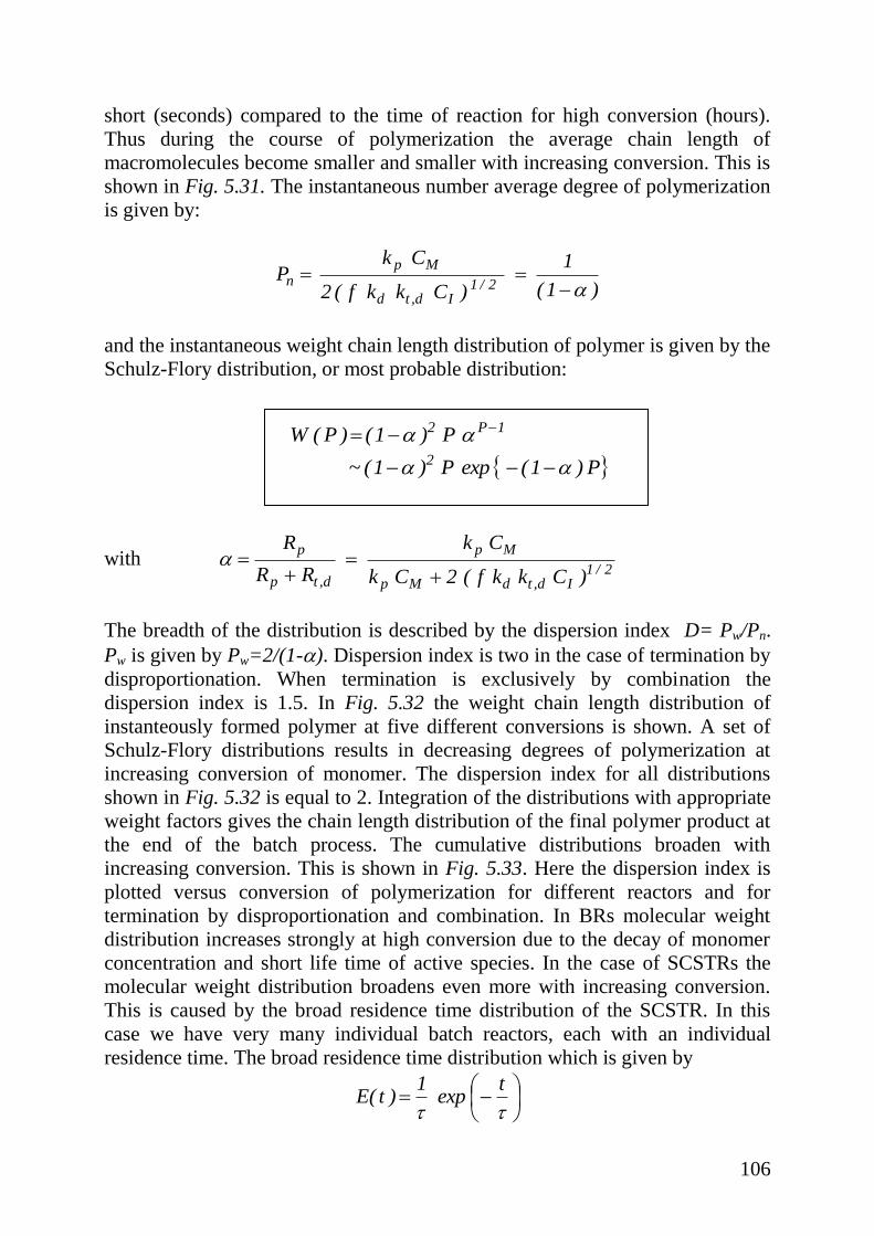
106
short (seconds) compared to the time of reaction for high conversion (hours).
Thus during the course of polymerization the average chain length of
macromolecules become smaller and smaller with increasing conversion. This is
shown in Fig. 5.31. The instantaneous number average degree of polymerization
is given by:
)1(
1
)Ckkf(2
CkP
2/1Id,td
Mpn
and the instantaneous weight chain length distribution of polymer is given by the
Schulz-Flory distribution, or most probable distribution:
1P2 P)1()P(W
P)1(expP)1(~ 2
with 2/1
Id,tdMp
Mp
d,tp
p
)Ckkf(2Ck
Ck
RR
R
The breadth of the distribution is described by the dispersion index D= Pw/Pn.
Pw is given by Pw=2/(1-). Dispersion index is two in the case of termination by
disproportionation. When termination is exclusively by combination the
dispersion index is 1.5. In Fig. 5.32 the weight chain length distribution of
instanteously formed polymer at five different conversions is shown. A set of
Schulz-Flory distributions results in decreasing degrees of polymerization at
increasing conversion of monomer. The dispersion index for all distributions
shown in Fig. 5.32 is equal to 2. Integration of the distributions with appropriate
weight factors gives the chain length distribution of the final polymer product at
the end of the batch process. The cumulative distributions broaden with
increasing conversion. This is shown in Fig. 5.33. Here the dispersion index is
plotted versus conversion of polymerization for different reactors and for
termination by disproportionation and combination. In BRs molecular weight
distribution increases strongly at high conversion due to the decay of monomer
concentration and short life time of active species. In the case of SCSTRs the
molecular weight distribution broadens even more with increasing conversion.
This is caused by the broad residence time distribution of the SCSTR. In this
case we have very many individual batch reactors, each with an individual
residence time. The broad residence time distribution which is given by
texp
1)t(E

107
leads to a very broad molecular weight distribution. The dispersion of the
distribution strongly increases with increasing conversion. In contrary to BR and
SCSTR, the HCSTR produces polymers with narrow molecular weight
distributions even at high conversion. The reason for this is the constant
monomer concentration at stationary state and the very short life time of active
sites. In this case residence time distribution does not affect the molecular
weight distribution of polymers. These simulations of a given polymerization
reaction run in different reactors have shown that the molecular weight
distribution of polymers formed can be very different from each other depending
on conversion of reaction.
However it must be mentioned that the effect of the reactor on the molecular
weight distribution of polymers is not always the same, but does depend on the
mechanism of the polymerization reaction. When chain transfer reactions play a
significant role completely different results may be seen with respect to the
molecular weight distribtution of polymers produced in a different reactor. This
has to be checked from case to case.
The next example is a condensation polymerization forming only linear chains.
If this type of polymerization reaction is run in a BR the conversion of
functional groups is defined as the fraction of functional groups that have
reacted at a given time:
0
0
N
NNp
and the degrees of polymerization are given by:
)p1(
1
N
NP 0
n
p1
p1Pw
The chain length distribution is given by:
1P2 pP)p1()P(W
and is again the Schulz-Flory distribution with a polydispersion index of two at
complete conversion of functional groups (D= Pw/Pn = 1+p). Fig. 5.34 shows
the increase of number average degree of polycondensation with conversion of
functional groups. Polymers of technical use with a degree of polymerization on

108
the order of 100 can only be produced at very high conversions. This can only
be done in an economical way in a BR or in continuous reactors with a plug
flow profile. In Fig. 5.35 the weight distribution of chain lengths is shown at
various conversions. Since in polycondensation reactions conversion can vary
from 0 to 1 the dispersion index varies from 1 to 2. This is different from free
radical polymerization. Here the dispersion index is always 2 because the
probability of propagation is always very close to unity. In single continuous
stirred tank reactors much broader molecular weight distributions do result as
shown in Fig. 5.36. This is due to the effect of the broad residence time
distribution. In polycondensation reactions the life time of growing chains is
extremely large and therefore the chain length distribution is affected by the
residence time distribution of the reactor. However these results are purely
theoretical results since HCSTR and SCSTR are not adequate reactors for
running polycondensation reactions at very high conversion, and on the other
hand many condensation and addition polyreactions are accompanied by side
reactions, which cause the formation of polymers with a Schulz-Flory
distribution.
Composition Distribution of Copolymers
Most of the polymers used are copolymers and not homopolymers. An exception
is poly(vinyl chloride), polystyrene and low density polyethylene. The
advantages of copolymers are the specific properties, which can be adjusted by
the monomers used and by the composition of copolymer and its distribution.
We have to distinguish between random, alternating, block, and graft copoly-
mers. Of special interest are random copolymers produced by free radical or
coordination polymerization. Since very often the reactivity of monomers can be
very different, special polymerization procedures have to be used in order to
produce copolymers with an equal distribution of monomers from chain to chain
and within a single chain.
Chemically uniform copolymers can be produced in batch or plug flow reactors
at high conversions only in the case of binary systems with copolymerization
parameters being equal and close to unity (r1=r2=1), or in the case of
copolymerization with an azeotropic point. This can be seen in Fig. 5.37. It
shows for three different binary systems the composition of copolymer formed
(expressed by the mole fraction F1 of monomer 1 in copolymer) in a batch
reactor as a function of monomer composition of charge f1 and of conversion.
The resulting distribution of copolymer composition can be seen in Fig. 5.38. In
general the copolymer composition distribution will be very broad in batch
reactors, since most of the industrially important copolymers are not systems
with r1 = r2=1, or with an azeotropic point at a certain composition of monomer.
The majority of comonomers have rather a very different reactivity of
copolymerization, and the result is a strong change of composition of monomer

109
mixture during the course of reaction in a batch or plug flow reactor, leading to
formation of very non-uniform copolymers with increasing conversion.
Copolymers of uniform composition can be produced in the case of monomers
with different reactivity by using the semi-batch technique, or running the
copolymerization in a mixed flow reactor. In the case of semi-batch copoly-
merization the less active monomer is introduced completely into the reactor and
the more reactive monomer is than added in such a way that the ratio of
monomer concentration is kept constant during polymerization. For this purpose
analytical sensors or reliable computer programs are necessary. More convenient
is the copolymerization in mixed flow reactors like the homogeneous continuous
stirred tank reactor. In a HCSTR operating at steady state monomer
concentration is constant in space and time. The result is therefore a chemically
uniform copolymer. The instantaneous copolymer equation
22221
211
212
111
frff2fr
fffrF
with 22,M1,M
1,M1 f1
cc
cf
and 22,M1,M
1,M1 F1
nn
nF
can be used for calculation of mole fraction of monomer 1 in the copolymer. cM,1
and cM,2 are the monomer concentrations in the exit stream of the reactor. In Fig.
5.39 the change in steady state copolymer composition is shown for the system
of styrene and acrylonitrile as a function of conversion. A copolymer with a
certain composition can be made either by varying the composition of feed at a
fixed conversion or by varying the extent of conversion at a given composition
of monomer feed.
However perfect mixing on a molecular scale cannot be realized in practise as
envisioned by the concept of a homogeneous continuous stirred tank reactor.
Most industrial reactors are not micro mixed, and the reaction mixture is
partially or fully segregated, especially at high viscosities. In the case of a
segregated continuous stirred tank reactor the copolymer composition
distribution will be much broader than in case of a HCSTR, and will broaden
with increasing conversion. It will be even broader than distributions of
copolymers produced in a BR. This again is the effect of the broad residence
time distribution of the SCSTR.

110
5.7 Reactor Scale-up
In general polymerization reactions are first run in lab scale reactors at certain
reaction conditions. If polymer properties fulfill the demand the same reaction is
then run in a larger scale reactor to produce more polymer for more intensive
testing. Scale-up of a reactor should be done by using reactors of the same
geometry. Geometric similarity means that all pertinent dimensions of reactors
should have a common constant ratio. For example the ratio of tank diameter to
stirrer diameter should be constant (see Fig. 5.40). Next step in scale-up of
polymerization reactors is the definition of parameters that must be kept
constant. Of special interest are parameters like :
- Mixing time for homogenization of miscible liquids
- Droplet diameter or specific interface of emulsions
- Distribution of polymer or catalyst particles within the reactor volume
- Mass transfer coefficient in heterogeneous systems
- Heat transfer coefficient of a reactor
These parameters may affect important polymer properties like particle size and
particle size distribution but also molecular weight and molecular weight
distribution. If the most important parameter is identified, then an appropriate
scale-up criterion has to be chosen. One of the oldest and most often applied
scale-up criterion is that of Büche, which says that the specific power input of
stirring should be kept constant during polymerization. Penney used different
scale-up criteria and plotted them in a diagram which is shown in Fig. 5.41 In
this logarithmic diagram the ratio of specific power input of stirring is plotted
versus the volumetric scale-up factor of a reactor. From this diagram it can be
seen that with the scale-up criterion of P/V = constant most of the named
process parameters can be kept constant. If for example the particle size of
monomer droplets (d32 ) should be the same in reactors of different size, then the
specific power input by stirring should be the same in each reactor. In the case
of mixing of liquids of low viscosity in the turbulent regime of flow, constant
mixing times can only be realized in the scale-up of reactors when stirring speed
is kept constant. This however means that specific power input by stirring must
be increased strongly with increasing volume of the reactor, and for economical
reasons this not the right thing to do. Thus, a somewhat larger time of mixing
has to be accepted in large scale reactors at constant specific power input.
The functional correlation of specific power input and volume of a reactor
shown in the Penney diagram shall be demonstrated in the case of mixing of
liquids.
If mixing in stirred tank reactors is performed in the laminar regime of flow,
then the following correlations are valid:

111
32 dN.constP and
.constN in the case of a helical ribbon.
If N is substituted by 1/ and 3d by V the following equation results when the
reaction mixture is the same in both reactors:
2
S
L
S
L
V/P
V/P
From this equation one can see that mixing time will be the same in both
reactors if the specific power input of stirring will be equal in both cases. If
mixing, however, is performed in the turbulent regime of flow a different
correlation results. In this case
53 dNNe P and
N constant for all types of stirrers
Again substitution of N by 1/ and with V~d3~D
3 in the case of reactors of
geometric similarity one gets the following correlation:
2
S
L
3
S
L
S
L
D
D
V/P
V/P
In this case the specific power input of stirring has to be increased according to
the second power of the ratio of reactor diameters if mixing time shall be equal
in both reactors.
5.8 List of Symbols
A Area, m2
Ar
Archimedes number, )r/(gdAr 23
C Concentration of chemicals, kmol/m3
D Diffusion coefficient, m2/s, or
Dispersion index of polymers
Da Damköhler number, 1n
0CkDa
Dr Diameter of reactor, m

112
d Diameter of agitator, m
dP Diameter of particle, m
d32 Sauter diameter of particle, m
dw Thickness of reactor wall, m
E Residence time distribution function, 1/s, or
Activation energy of reaction, J/mol
F Mol fraction of monomer in copolymer
f Mol fraction of monomer in monomer mixture, or
Efficiency factor of initiator
Fr Froude number, Fr = u0 /(dg)
g Standard gravity, m/s2
h Heat transfer coefficient, W/(m2K)
H Enthalpy, J/mol
k Rate constant of chemical reactions and mass transport processes
MM Molecular weight of monomer, kg/k mol
MT Torque acting on stirrer shaft, Nm
m Weight, kg
m Weight flux, kg/s
N Number of revolutions of stirrer, 1/s, or
Number of functional groups, or
Number of reactors in a cascade
Ne Newton number, )dN/(PNe 53
Nu Nusselt number, /DhNu r
Nseg Number of segregation,
n Molar flux, mol/s
P Power input of stirrer, W
Pn Degree of polymerization, number average
Pw Degree of polymerization, weight average
Pr Prandtl number, /cPr p
p Degree of conversion in condensation polymerization
Q Heat flux, W
Q Gas flow number, )dN/(gQ 3
g Gas flow rate, m3/s
R Rate of reaction, kmol/(m3s)
R Gas constant, J/(molK)
r Copolymerization parameter
Re Reynolds number, /dNRe 2
Sc Scmidt number, Sc=/D
Sh Sherwood number, D/dkSh Ps
T Temperature, K or 0C

113
t Time, s
U Overall heat transfer coefficient, W/(m2K)
u Linear velocity, m/s
u0 Superficial gas velocity, m/s
V Volume, m3
V Volumetric flux, m3/s
X Conversion
Probability factor
Shear rate, 1/s
Thickness of layer, m
Specific energy input, W/kg or m2/s
3
Dynamic viscosity, Pa s or kg/(ms)
Mixing time, s
Thermal heat conductivity parameter, W/(mK)
or micro scale of turbulence, m
Kinematic viscosity, m2/s
Density, kg/m3
Interfacial tension, N/m or J/m2
Average residence time, s
Volume fraction,
5.9 References
- S. Nagata: „Mixing, Principles and applications“, Halsted Press, John Wiley
and Sons, 1975
- J.Y. Oldshue: „Fluid Mixing Technology“, McGraw-Hill Publications, 1983
- F.A. Holland and F.S. Chapman: „Liquid Mixing and Processing in Stirred
Tanks“, Reinhold Publishing, 1966
- L.M. Rose: „Chemical Reactor Design in Practice“, Elsevier, 1981
- H.S. Fogler: „Elements of Chemical Reaction Engineering“, Prentice-Hall
International, 1999
- T. Grewer: „Thermal Hazards of Chemical Reactions“, Elsevier, 1994
- K.H. Reichert and H.U. Moritz: „Polymer Reaction Engineering, in
Comprehensive Polymer Science, Vol. 3, Part I, page 327, Pergamon Press,
1989
- M. Zlokarnik: „Dimensional Analysis and Scale-up in Chemical Engineering,
Springer, 1991

114
5.10 Tables and Figures
Batchwise
Advantage: ideal for small-scale production, very
flexible, multi purpose application, high conversion
obtainable.
Disadvantage: large cycle time, dangerous process,
concentration gradients may affect polymer quality,
temperature control can be difficult with fast exotermic
reactions.
Semi-batchwise
Advantage: good control of reaction rate and product
quality (copolymer composition), relative safe process,
high yield by shifting the chemical equilibrium
(polycondensation), stationary concentration of
reactants.
Disadvange: lower performance than batch reactor,
extra devices for pumping and controlling.
Continuous
Advantage: ideal for large quantities of polymers with
constant quality, high degree of automation, relative
safe process, high reactor performance.
Disadvantage: process is not flexible, expensive instru-
mentation (pumps, sensors, controllers), high costs for
maintenance.
Tab. 5.1: Mode of operation of stirred tank reactor

115
Agitator Diameter
Ratio
Baffles Tip Speed
(m/s)
Polymerization
Method
Turbine
Propeller
0.3
0.3
yes
yes
3 – 12
3 – 12
Emulsion
Suspension
Blade
Intermig
(Ekato)
0.5
0.7
yes/no
yes/no
1 – 10
1 – 10
Solution
Suspension,
Slurry,
Solution
Helical Ribbon
Helical Screw
0.9
0.9
no
no
0.5 – 2
0.5 – 2
Solution ( > )
Bulk (>> )
Tab. 5.2: Agitators used for different methods of polymerization.
Agitator/Reactor
Reactor Conversion Reaction Volume
BR Daexp1 X
XCM
ttmV
0,MM
deadP
HCSTR Da1
11X
X1CMk
mV
0,MM
P
Cascade
N
N
Da1
11X
XCMk
]1X1[NmV
0,MM
N/1
P
Tab. 5.3: Conversion and reaction volume of different stirred tank reactors.
Correlations refer to polymerization reaction of first order

116
Reaction HCSTR SCSTR
O. Order
(Da = k / CM,0)
DaX
Da
1expDaDaX
1. Order
(Da = k) Da1
11X
Da1
11X
Tab. 5.4: Conversion equations of segregated (SCSTR) and non-segregated (HCSTR)
reaction systems of zero- and first-order reactions

117
Fig. 5.1: Some major types of agitators and viscosity ranges of application
Fig. 5.2: Axial and radial flow patterns in stirred tank reactors equiped with baffles

118
Fig. 5.3: Power input characteristic of different stirrers with and without baffles for
homogeneous Newtonian liquids
Fig. 5.4: Mixing time characteristic of different types of agitators for Newtonian
liquids of similar density and viscosity
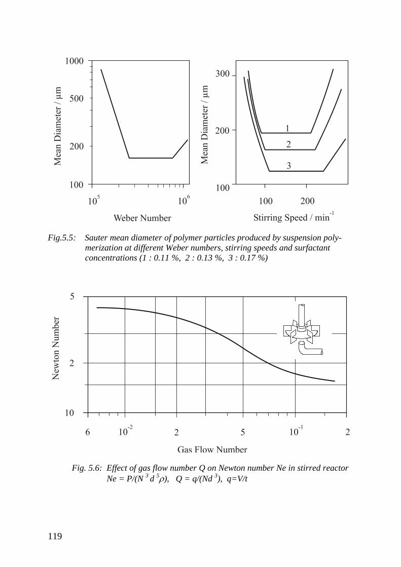
119
Fig.5.5: Sauter mean diameter of polymer particles produced by suspension poly-
merization at different Weber numbers, stirring speeds and surfactant
concentrations (1 : 0.11 %, 2 : 0.13 %, 3 : 0.17 %)
Fig. 5.6: Effect of gas flow number Q on Newton number Ne in stirred reactor
Ne = P/(N 3 d
5), Q = q/(Nd 3), q=V/t

120
Fig. 5.7: Effect of specific power input on liquid-side mass transfer coefficient in
bubble column reactor filled with different liquids containing polyethylene
particles
Fig. 5.8: Distribution of glass beads in stirred tank reactor at different stirring
speeds

121
Fig. 5.9: Comparison of mixing effectiveness of different agitators at different power
input
Fig. 5.10: Calculated mass transfer coefficient for spherical particles of different size
settling at terminal velocity in a liquid

122
Fig. 5.11: Different methods of heat removal from stirred tank reactor
Fig. 5.12: Decrease of heat transfer coefficient and increase of viscosity with
conversion of solution polymerization in a stirred tank reactor (helical
ribbon agitator, 160 rotations per minute)

123
Fig. 5.13: Effect of stirring speed on cooling capacity of stirred tank reactor

124
Fig. 5.14: Stability diagram of reactor at stationary state with = 388 min
Curve a: heat production
Curve b: heat removal
Fig. 5.15: Transition characteristic of operating point at an increase of jacket
temperature from 85 to 870C at time zero

125
Fig. 5.16: Temperature run away phenomena at different failures of operation
a : monomer feed and cooling fail completely
b : monomer feed stops but cooling by jacket works
Fig. 5.17 Tracer concentration-time correlation of a pulse experiment

126
Fig. 5.18: Transforming the experimental concentration curve into the exit age
curve E
Fig. 5.19: Tracer concentration-time correlation of a step experiment
Fig. 5.20: Transforming the experimental tracer concentration curve into the F
curve (transition function)
M
vCF

127
Fig. 5.21: RTD of a cascade of equal sized stirred tank reactors (with N=1, 5 and )
F
t
E
t
E

128
Fig. 5.22: Compartment models for stirred tank reactors with dead zone (left)
and bypass (right)
v Vm
Vd
v va
vb
V
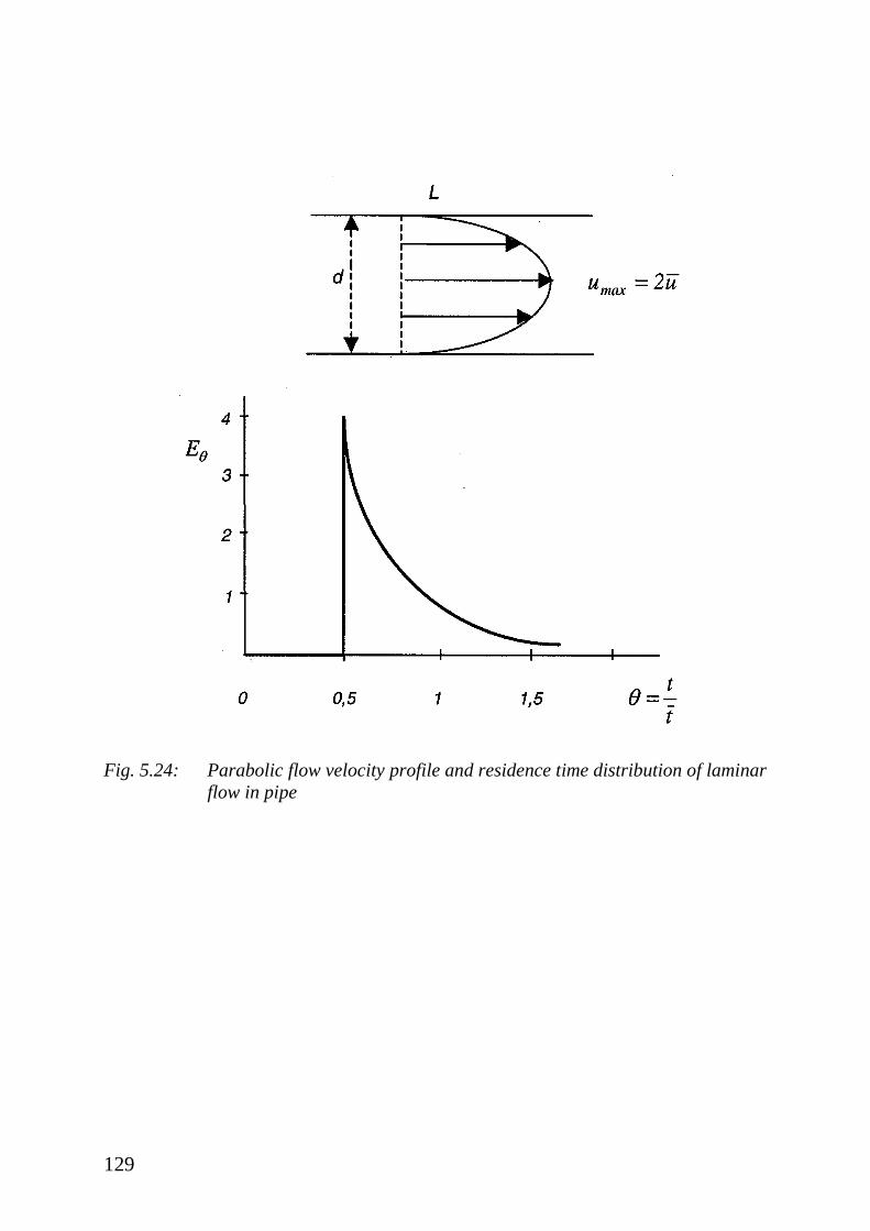
129
Fig. 5.24: Parabolic flow velocity profile and residence time distribution of laminar
flow in pipe

130
Fig. 5.25: Dimensionless conversion-time correlations of different stirred tank
reactors for 1. order polymerization reaction with k = 10-4
s-1
Fig. 5.26: Reactor capacity of different stirred tank reactors as function of time and
conversion. First order polymerization with CM,0 = 5 mol/l and k=10-4
s-1

131
Fig. 5.27: Concentration profiles and residence time distribution of different
stirred tank reactors
Fig. 5.28: Effect of segregation on conversion. Polymerization reaction of
0. and 1. order

132
Fig. 5.29: Compartment model of a continuous stirred tank reactor and the
correspondinng residence time distribution (CSTR)
Fig. 5.30: Effect of volume fraction of dead water and plug flow on relative
conversion of stirred tank reactor at two different reference con-
versions (0.2 and 0.8)

133
Fig. 5.31: Relative cumulative degree of polymerization (weight and number
average) as function of conversion of free radical polymerization
without chain transfer reactions
Fig. 5.32: Weight distribution of chain length of instantaneously formed polymer by free radical polymerization in batch reactor at small conversion increments

134
Fig.5.33: Dispersion index (D=Pw / Pn) of polymers produced by free radical
polymerization in different stirred tank reactors as function of conversion
(dotted line: termination by disproportionation, solid line: termination by
combination)
Fig.5.34: Cumulative degree of polymerization as function of conversion of conden-
sation polymerization

135
Fig.5.35: Molecular weight distribution of polymer formed by condensation
polymerization in a batch reactor
Fig. 5.36: Dispersion index D =PW/PN as a function of degree of condensation
polymerization in different reactors

136
Fig.5.37: Composition of the copolymer produced in a batch reactor as function of
monomer composition of charge as well as conversion
First column: instantaneous composition; second column: instantaneous
compositions, starting with cM,1:cM,2=1:3, 1:1 and 3:1; third column: cumu-
lative compositions based on the same starting ratios
Fig. 5.38: Copolymer composition distributions of different pairs of monomers.
Complete polymerization in a batch reactor for three different molar ratios
of monomer (CM,1 : CM,2 = 1 : 3 (first column) 1 : 1 (second column) and
3 : 1 (third column) F1 : mol fraction of monomer 1 in the copolymer)

137
Fig.5.39: Continuous copolymerization in a stirred tank reactor of styrene (f1=0.4)
and acrylonitrile(f2=0.6). Composition of accumulated copolymer F1 and F2
as a function of conversion
Fig. 5.40: Scale-up of stirred tank reactor

138
Fig. 5.41: Penney diagram with different scale-up criteria

139
6. POLYMERIZATION PROCESSES
6.1 General Aspects
Chainwise polymerization reactions are characterized by the following features:
- Strong increase in viscosity of a reaction mixture during the entire course of
polymerization
- Kinetics of reaction can be very sensitive with respect to small amounts of
impurities like free radical scavangers or catalyst poisons
- Non-uniform polymers are formed due to the mechanism of polymerization
- Polymerization reactions are strongly exothermic and in general non rever-
sible at reaction conditions
Stepwise polymerization reactions are in general reversible reactions. The
viscosity of the reaction mixture increases strongly only at very high conversion
of functional groups. Typical condensation reactions are relatively slow running
reactions with low reaction enthalpies. They have to be run at high conversion in
order to get polymers with high molecular weight. Another important parameter
which also affects molecular weight is the exact stoichiometry of functional
groups. The stoichiometry of reactants must be carefully controlled.
Industrial polymerization processes are in general continuous processes run at
constant temperature and pressure. The structure of a typical polymerization
process is characterized by physical and chemical treatment steps (see Fig. 6.1).
The materials entering the polymerization process undergo first a number of
physical treatments like purification, mixing, heating, or cooling. Then the
monomers are polymerized in a suitable reactor at certain reaction conditions.
After chemical reaction the reaction mixture is again treated in physical ways in
order to recover the polymer in such a form and quality as demanded by
customers.
Purification of monomers and solvents for chainwise polymerization focuses on
the removal of traces of free radical scavangers and catalyst poisons. In general
separation processes like distillation and adsorption are used for this purpose. In
the case of stepwise polymerization the complete removal of monofunctional
monomers is of interest, otherwise no polymers with high molecular weight can
be produced.
Purification of polymers at the end of a polymerization process deals with the
removal of unreacted monomer from the polymer. The effective removal of
monomer from the polymer is a demanding task. Heating, evaporation, and
effective mixing of polymer are the appropriate procedures of purification.
Effective compounding of polymers with property improving additives at the
end of a polymerization process is also an important polymer treatment step. In
general extruders are used for this purpose.

140
The development of a new polymerization process starts with the choice of the
chemical polymerization reaction for synthesis of a wanted polymer product.
Today especially coordination and condensation or addition polymerization
reactions are of special interest. These reactions allow the synthesis of polymers
with a special architecture or special chemical composition. The next step in
process development is the choice of a suitable polymerization procedure.
Polymerization in heterogeneous systems can have some advantages in
comparison to homogeneous systems, like better mixing of a reaction mixture or
better heat removal due to lower viscosities. From a commercial point of view
the bulk phase polymerization is a suitable process since no solvent or diluent
has to be used. Mixing and heat removal however can cause problems. The next
stage in process development is the choice of reactor type and its mode of
operation.
In the case of continuous polymerization process the residence time distribution
of reactor can have an effect on reactor performance and polymer quality. Very
often a cascade of reactors is used. The polymerization reactor is the heart of a
polymerization process, but the right choice of appropriate physical treatment
steps before and after chemical reaction can also have a large impact on
performance of a polymerization process. In Tab. 6.1 the different steps of
process development in polymer production are summarized. In general the type
and amount of polymer to be produced will be given. Decisions have to be made
on the type of polymerization reaction, method of polymerization, conditions of
polymerization, type of reactor, and on the type of unit operations.
6.2 Processes for Chain-Growth Polymerization
Solution Polymerization/High Density Polyethylene
For polymerization in solution good solvents have to be used to dissolve the
monomer and also the polymer formed. The solvent should be chemically inert
and easy to recover after polymerization. The advantage of polymerization in
solution is the lower viscosity of reaction mixture than in bulk polymerization in
the absence of a solvent. By this means good control of mixing and heat removal
is possible. Initiator or catalyst efficiency can also be better than in
homogeneous bulk polymerization due to better agitation of the reaction
mixture. Disadvantages of solution polymerization are the costs for removal and
recovery of solvents and the tendency of formation of polymer deposit on the
wall of the reactor. The scale of polymer on the walls of the reactor has to be
removed in order to maintain good heat transfer and avoid inclusion of gelled
polymer in the final product. Polymers are recovered from solution
polymerization by flushing off the solvent. The polymer formed is in general a
fluffy powder which must be compacted in separate melting and granulation
process. Major polymers produced by polymerization in solution are high

141
density polyethylene, 1,4-cis-polybutadiene and polystyrene. Hexane is used in
general in the case of ethylene and butadiene polymerization. But also bulk
polymerization of ethylene at high pressure and temperature must be regarded as
solution polymerization in a homogeneous medium since the polymer formed is
completely dissolved in its own monomer at the reaction conditions given.
In Fig. 6.2 the flow diagram of solution polymerization process of ethylene with
Ziegler-Catalysts is shown. Ethylene, a comonomer, and hexane are mixed in an
absorber at low temperature. Then the solution is cooled down to -40 0C and
pumped into the stirred tank reactor together with the catalyst solution. The
polymerization is run in the temperature range of 130 to 2500C to keep the
polymer formed in solution. The corresponding pressure is in the range of 30 to
200 bar. The mean residence time of the reaction mixture is on the order of 10
minutes. This corresponds to a conversion of monomer of about 95%. The
concentration of polymer in solution is about 5 to 10 wt % and affects strongly
the viscosity of the reaction mixture. The viscosity is also affected by the
molecular weight of polymer. The molecular weight of polymer is controlled by
the temperature of polymerization. The viscosity is controlled on-line during the
course of polymerization. After passing the reactor the reaction mixture is
pumped into a flash tank where solvent and monomer are removed partially
from the reaction mixture by evaporation and desorption. The concentrated
polymer solution is then pumped into a mixer and mixed with additives like
stabilizers, pigments, processing agents, and so on. Then the concentrated
polymer solution is pumped into a second flash tank where most of the solvent is
removed. Finally, the polymer melt is transfered into an extruder where it is
mixed with further additives and degassed. At the exit of the extruder the
polymer melt is cut by a rotating knife and simultaneously cooled down by
rinsing with water. After drying, the polymer granules are ready for packaging.
The production performance of a solution process is due to the high rate of
polymerization, with approximately 1 kg of polymer produced per liter of
reactor volume and hour at 1300C. The polymer produced is characterized by
relatively low molecular weight and narrow molecular weight distribution, and
therefore used as material for injection moulding processing.
Suspension Polymerization/Poly(vinyl chloride)
Suspension polymerization is a water-cooled bulk polymerization. Liquid
monomer with dissolved initiator is dispersed in water by vigorous stirring. The
droplets formed are transformed during polymerization into sticky, highly
viscous particles, which become rigid and have diameters in the range of 100 to
1000 m. To prevent coalescence of the sticky particles during the course of
polymerization proper stabilizing agents have to be used. In general water
soluble natural or synthetic polymers are used, like cellulose derivatives or
poly(vinyl alcohol). Proper agitation of the reaction mixture is important since
the monomer is less dense than water while polymer is in general more dense

142
than water. The viscosity of the heterogeneous system remains fairly constant
during a polymerization reaction and is determined mainly by the water phase,
but also by the volume fraction of polymer. The final reaction mixture typically
contains about 30 volume percent of polymer. Suspension polymerization is the
only procedure of polymerization which cannot be performed in a continuous
way. In industry up to now only batch processes are known. This is mainly due
to the tendency of the reaction mixture to form deposits of polymer on the wall
of reactor. This fact prevents any continuous processing since polymerization
must be stopped too often for cleaning of reactor.
Suspension polymerization is applied in industry for production of poly(vinyl
chloride), expandable polystyrene, and high impact polystyrene. The major
process for poly(vinyl chloride) production is suspension polymerization. In Fig.
6.3 the flow diagram of the poly(vinyl chloride) suspension polymerization
process is given. It is a batch process with cycle times of less than 8 hours.
Liquid vinyl chloride and water with dissolved surfactant and initiator are fed
into the stirred tank reactor which can have a volume up to 200 m3. Then the
reactor content is heated up to temperatures in the range of 50 to 700C, resulting
in pressures of 8 to 12 bar. Very often steam is used for direct heating of the
reaction mixture. The temperature of reaction determines the molecular weight
of polymer formed. The higher the temperature the higher the rate of initiator
decomposition and the lower the molecular weight of the polymer formed. The
effect of temperature of reactor and jacket as well as pressure are given in Fig.
6.4 for a typical batch polymerization of vinyl chloride in suspension. From the
differences of temperatures one can see that the rate of heat production, resulting
from rate of polymerization, is increasing with increasing conversion and
reaches a maximum value at a conversion of about 70%. Then the rate of
polymerization falls. Simutaneously the pressure of the reactor is falls. This is
the stage of polymerization where vinyl chloride is no longer present as a
separate liquid phase. The rest of vinyl chloride is completely absorbed by the
polymer produced. Heat of reaction is removed by the cooled jacket of the
reactor and also by an external heat exchanger via evaporation and condensation
of vinyl chloride. At about 90% conversion, which is measured by calorimetry,
the reaction is stopped. The hot suspension is filled into a storage tank and from
there pumped into a degasifier to remove the vinyl chloride left in the polymer
particles. This is done by heating and applying vacuum. After an intensive
demonomerization of the polymer the suspension is conveyed into a continuous
centrifuge. The wet product (20 to 30% water) is then dried first in a pneumatic
dryer and then in a fluidized-bed dryer by using hot air. To remove small
polymer particles from the air passing through the dryers, cyclones and gas
filters are used. One major parameter of the polymer produced is the porosity of
the particles, which is responsible for the absorbing capacity of the particles
with respect to liquid plasticizers. The absorbing capacity of the polymer
particles can be influenced by the kind of surfactants used for stabilizing the

143
monomer droplets. The size of the particles formed is affected by the physical
properties of the monomer/water emulsion (surface tension, viscosities,
densities), by the polymerization conditions (stirring speed, temperature,
concentration of chemicals), and by the geometries of the reactor and stirrer
used.
Emulsion Polymerization/Styrene-Butadiene-Copolymer
The most important process for production of synthetic rubber based on styrene
and butadiene copolymers is the emulsion polymerization. Emulsion poly-
merization is also used for production of poly(vinyl chloride) and acrylo nitrile-
butadiene-styrene copolymers. The advantages of emulsion polymerization are:
- Low viscosity of the reaction mixture during the entire course of
polymerization.
- Polymers with high molecular weight are formed at high rates of polymeri-
zation.
- Highly concentrated polymer latex is formed which can be used directly for
further applications.
These benefits make emulsion polymerization a frequently used process of
polymer production in free radical polymerization. The polymer particles of the
latex produced are normally in the range of 100 nm in diameter and the latex
contains in general 50% polymer. In Fig. 6.5 the flow diagram of an emulsion
polymerization process for production of styrene-butadiene copolymer is shown.
Since polymerization is run at 50C the rubber produced is called “cold“ rubber
and is characterized by a relatively high content of trans-1,4- butadiene units,
which has a positive effect on some technological properties of the rubber. The
process starts with the emulsification of monomers and molecular weight
modifiers in water with dissolved emulsifiers, which are in general natural
soaps. The emulsion is than cooled down to 50C and the redox initiator is added.
First the reducing agent (sodium formaldehyde sulfoxylate), then the
hydroperoxide is added. The polymerization is performed in a series of six to ten
well agitated reactors. Since the reaction temperature greatly influences polymer
properties, the heat removing system must be well designed. In general heat is
removed by evaporation cooling of ammonia, which is pumped through coils
placed within the reactors. After an average reaction time of 8 to 10 hours the
polymerization reaction is stopped at a conversion of 60 to 70%. At higher
conversions polymer properties would be affected in a negative way due to
formation of long chain branching and crosslinking. The latex is then flashed
into two drums. The first one being at atmospheric pressure and the second one
working under vacuum. In these drums butadiene is removed. The latex is then

144
pumped to the top of a stripping column operating in vacuum. The latex passes
downward over perforated plates counter-current to steam. The monomer-free
polymer dispersion is then mixed with additives like carbon black, oil,
antioxidant and then pumped into a coagulation tank where acid (H2SO4) and
brine (Al2(SO4)3) is added. Coagulation usually takes place in two well-agitated
vessels. During this operation the rubber is precipitated in the form of porous
crumbs, which are washed free of salt and acid and then dried and baled.
Slurry Polymerization Process/High Density Polyethylene
The polymerization of olefins in a suspension or slurry is a suitable process for
production of polyolefins like polyethylene and polypropylene. The
polymerization is catalysed by different types of heterogeneous catalysts
dispersed in an inert liquid, like hydrocarbons with low boiling points. The
polymer formed is insoluble in the liquid phase at the polymerization
temperature. It forms particles with morphologies which are more or less a
replication of the catalyst particles. The major advantage of a slurry
polymerization process is the relative low viscosity of the reaction mixture,
which favours good mixing and heat removal in the reactors used. Stirred tank
and loop reactors are used in general, with reactor volumes up to 100 m3. The
reactors are run at pressures of 10 to 20 bar and temperatures of 80 to 1000C.
The average residence time in stirred tank reactor is 2 to 3 hours and in loop
reactors 0.5 to 2 hours. The performance of reactors is in general controlled by
the process of heat removal. The slurry leaving the reactor has a solid content of
about 50 wt %. Unit operations for isolation of the polymer are centrifugation,
steam stripping, and drying of the powder. The powder is then mixed with
additives and granules are formed by using extruders. The molecular weight of
the polymer is controlled by hydrogen or by temperature. The distribution of the
molecular weight can be controlled by the nature of the catalyst used or by
means of process technology, like using a train of reactors run at different
reaction conditions. Small amount of comonomers are used to modify the
density of the polymer and to increase the toughness or resistance to stress
cracking.
In Fig. 6.6 the flow diagram of a slurry polymerization process for polyethylene
production is given. It is based on developments of former Hoechst company.
The ethylene used for polymerization is in general supplied by modern plants in
such a quality that it may be polymerized with little or no further purification. In
Tab. 6.2 the specification for such a polymerization grade ethylene is given.
Commercial catalysts for polymerization of olefins are in generel heterogeneous
catalysts. The catalytic active complexes are fixed on the surface of appropriate
supports, which are porous particles with diameters in the range of 50 to 100
m. These catalyst particles are first dispersed in a diluent and then pumped into
the reactor with such a rate that the performance of the reactor is kept at a

145
constant level. Pressure and temperature are also kept constant during
polymerization. In Fig. 6.6 only one reactor is shown but also two or more
reactors in series are used. The slurry is passed into a pressure release vessel
where most of the ethylene is removed and then pumped into a centrifuge to
remove most of the diluent from the polymer. The diluent is recycled directly to
the reactor. The polymer is transferred from the centrifuge into a stripper, where
the rest of the diluent is stripped off the polymer by using steam, which is blown
into the stirred product. After a second centrifugation step the wet product is
dried in a fluidized-bed drier using hot air. Additives are then added to the
polymer powder in a mixer, and this mixture is then pelletized in an extruder
and finally dried in a moving bed dryer.
Gas Phase Polymerization Process/High Density Polyethylene
Gas phase polymerization is applied only for production of polyolefins like
polyethylene and polypropylene or copolymers of ethylene and propylene by
using heterogeneous catalysts with particle diameters of about 50 m. Gas phase
polymerization processes are relatively simple processes, particularly if the
customers are able to use the directly produced polymer particles without any
pelletization process. A further advantage of the process is that no diluents are
used. Since the process operates close to the melting point of the polymer,
accurate temperature control is necessary, and is done by regulating the rate of
catalyst addition into the reactor. If a thermal run away polymerization is
detected, carbon dioxide can be injected into the reactor to poison the catalyst.
Problems may also arise if polymer films are formed on the surface of reactor
due to electrostatic charge of the fluidized particles. In Fig. 6.7 the flow diagram
of the gas phase polymerization process for high density polyethylene
production is shown. Ethylene, comonomer, hydrogen, and catalyst are injected
into a fluidized-bed reactor. The reaction zone is the lower part of the reactor. In
the upper expanded section of reactor the gas velocity is lowered, allowing the
particles to fall back into the reaction zone. The lower part of the reactor has a
diameter of about 4 m and a height of 10 m. The overall height of the reactor is
ca. 30 m. The gas phase enters the reactor through a distributor plate, which
manages an even distribution of the gas phase across the cross-sectional area of
reactor. The reactor operates at 80 to 1000C and a pressure of 20 bar. The
average residence time of the particles is 3 to 5 hours. The residence time
distribution corresponds more or less to a continuous stirred tank reactor with
back mixing of material and heat throughout the total reaction zone. The
conversion of monomer per pass of reactor is ca. 2%. Heat removal takes place
more or less by the circulating gas phase. The gas flow necessary for heat
removal is given by following equation:

146
Tc
HmV
p
R
with m being the production rate of polymer, HR is the reaction enthalpy of
polymerization, and cp are the density and specific heat capacity of the gas
phase, and T is the temperature difference of gas phase before entering the
reactor and the reaction temperature. The recycled gas flow is cooled down by
passing through a gas cooler before entering the reactor. Polymer particles are
taken out of reactor by a sluice working in short intervals via sequenced valves.
The polymer powder passes a cyclone, from which residual monomers are
recovered. Then it is recompressed and transferred back into the main pipeline
of monomer. The polymer powder flows from the cyclone into a purge tank
where final amounts of monomers are removed from the product.
6.3 Processes for Step-Growth Polymerization
In typical step-growth polymerization reactions like polyester or polyamide
synthesis the growth of macromolecules is a relatively slow process compared to
chain-growth polymerization reactions. The activation energies of these step
growth reactions are in the order of 85 kJ/mol. To accelerate the rate of reaction
catalysts and elevated temperatures are used. The enthalpy of polyester or
polyamide synthesis is relatively low at –10 to –20 kJ/mol. In this case heat
removal is not a problem. When these kinds of condensation reactions are
accelerated by application of heat and catalysts, depolymerization reactions
become important. This will affect the conditions under which the reactions are
carried out. Since step-growth polymerization reactions have unfavorable
equilibrium constants it is therefore customary to operate the process at high
temperatures and reduced pressure to remove condensation products like water
or alcohol from the reacting system. Very high conversions have to be achieved
in order to get polymers with high molecular weights suitable for technical
applications.
The rate of condensation polymerization is often limited by the rate of transfer
of condensation products like water or alcohol from the liquid, or the solid phase
into the vapor phase. A kinetic model must then include both the kinetics of the
chemical reaction and mass transfer. Mass transfer will strongly depend on
reactor design and operation conditions like stirring.
But step-growth polymerization reactions can also be very fast and very
exothermic reactions. The synthesis of polyurethanes or phenol-formaldehyde
resins are examples of such reactions. In this case lower reaction temperatures
are applied.
The following examples of step-growth polymerization processes will refer to
the synthesis of linear and crosslinked products. Linear polymers are

147
thermoplastic materials, crosslinked polymers are non-meltable materials at their
final stage of production.
Condensation Polymerization in Solution/Phenolic resins
An important type of polymers produced by step-growth polymerization are
nonlinear polymers formed by condensation polymerization of monomers with
more than two functional groups per molecule. One major type of network
polymers are the phenolic resins. Phenolic resins are polycondensation products
of phenol and formaldehyde. The ring hydrogens in para- and ortho-position of
the phenol molecule can react with formaldehyde to form hydroxymethyl-
substituted phenols which can then start condensation reactions with the
formation of methylene bridges or dimethylene ether bridges and elimination of
water. The production of phenolic resins is stopped at a stage where oligomers
are formed, which are thermoplastic materials and can be cured afterwards
during processing in molds. Phenolic resins are classified as novolacs and resols.
They have different curing properties and are used in different applications. The
production of phenolic resins takes place in general in batchwise processes
because a very great variety of types are produced in relatively small quantities.
The phenolic resin plant shown in Fig. 6.8 can be used for all steps in batchwise
production. Phenol in the molten state is fed into the reactor first and catalyst
and formaldehyde dissolved in water (30 w-%) are then added. The rate of
formaldehyde addition is controlled depending on the heat evolved. Substitution
and condensation reactions between phenol and formaldehyde are strongly
exothermic with about -99 kJ/mol and can proceed very vigorously. Therefore
appropriate cooling is important. Cooling is done by evaporation of volatile
liquids. The temperature of reaction is either 60 or 1000C, depending on
synthesis of resols or novolacs. At the end of the reaction the volatile parts of the
reaction mixture are distilled off under reduced pressure. The molten resin as
residue is then removed from the reactor. Rapid emptying of the reactor and
cooling of the resin is important to avoid further condensation of the product.
Cooling is done in a cooling conveyer filled with water. The product is then
milled, sieved, and mixed with different additives and fillers.
Condensation Polymerization in Melt and Solid State/Poly(ethylene terephtha-
late)
In Fig. 6.9 the flow diagram of continuous polymerization process for
production of poly(ethylene terephthalate) is shown. Dimethyl terephthalate,
ethylene glycol and catalysts are fed into a series of Robert-evaporators in which
the ester interchange reaction takes place at temperatures of 150 to 2100C and
atmospheric pressure. Bis (hydroxyethyl) terephthalate and methanol are formed
primarily. Methanol and ethylene glycol emerging from the reactors are passed
through a rectifying column and ethylene glycol is fed back into the reactors. At

148
a conversion of about 90 to 95%, which is achieved at a hold up time of 4 to 6
hours, the reaction mixture is transferred into the first stage of a condensation
polymerization unit. The reaction mixture consists of oligomers, mainly dimers
and trimers. In this series of stirred tank reactors the temperature is increased to
265-2850C and the pressure is lowered to about 50 mbar to keep the
condensation fast and the reaction mixture molten. After a hold-up time of 2 to 3
hours, which corresponds to a conversion of functional groups of about 0.95 to
0.97, the melt with a degree of polymerization of 20 to 30 is passed into a
rotating disc reactor. In this reactor the pressure is lowered even further to 1
mbar in order to remove ethylene glycol almost completely from the polymer
melt. The reaction temperature is kept at 265 to 2850C. The reaction rate is
controlled by mass transfer limitation. After a residence time of 2 to 3 hours the
polymer melt leaves the rotating disc reactor with a number average degree of
polymerization of about 120, which corresponds to a conversion of functional
groups of 0.99. To attain even higher molecular weights the products may be
subjected to solid-state post condensation within moving bed reactors at 2500C
for 20 hours. The reactor is then purged with nitrogen gas or put under vacuum.
The direct esterification of terephthalic acid with ethylene glycol is gaining
more importance because of some advantages like better polymer properties, no
usage of catalyst, and no handling of methanol.
Addition Polymerization in Liquid Medium Polyurethanes
Polyurethanes are produced either by the so called prepolymer process or by the
one-shot process. In case of the prepolymer process a diol is reacted with an
excess of a diisocyanate. The prepolymer formed contains an excess of
isocyanate groups which are reacted in a second step with low molecular weight
diols, diamines, or water to form the final end product. The polyurethanes
formed are two phase systems containing hard and soft domains. In general they
are used as elastomers.
The one-shot process is a much more simple process. In this case all reaction
components are well mixed simultaneously and react with each other in a rather
short time to a nearly complete conversion. If the reacting partners have the
same reactivity the polyurethanes formed have a statistical composition of the
two monomer units. The one-shot process is used in general for production of
polyurethane foams. The fundamental reaction in this case is the reaction of the
isocyanate group with water. The resulting carbon dioxide is used as the foam
formation agent.
In Fig. 6.10 the flow sheet of a foam forming plant is shown. The process
consists of two storage vessels, which can be heated. In one vessel polyol,
catalyst, surfactant, foaming agent and other additives are placed. The other
vessel contains the multifunctional isocyanate. Both reaction mixtures are in the
liquid state at reaction temperatures above 500C. Before injecting the liquids into
the mixing head the feed streams are first recycled by using accurate dosing

149
pumps. When the right feed ratio is adjusted the fluids are pumped into the
mixing chamber via nozzles, and are well mixed by the turbulence created in a
very short time. The further processing of the reaction mixture depends on the
product to be produced. In case of foam slabs or blocks the reaction mixture is
sprayed on a circulating band.
If the reacting components are very reactive the so called technique of reaction
injection molding (RIM-technique) can be used for production of moldings of
different shape. In this case the exit of the mixing chamber is pressed against the
entry of the mold and the reaction mixture is injected into the mold. The entire
polyurethane formation is completed within a few minutes. The mold is then
split open to discharge the final product. So called integral foams are obtained if
the foaming process is controlled so that moldings are produced that have a
closed surface and a cellular core. The mixing head of the reaction injection
molding plant is a very sophisticated part of the plant. The sketch of a pressure
controlled mixing chamber is shown in Fig. 6.11. The upper sketch shows the
mixing chamber at mixing conditions. The lower sketch refers to the state of
cleaning of the mixing head.
6.4 References
- „Ullmann´s Encyclopedia of Industrial Chemistry“, Vol A 21 and 23,VCH,
1992
- „Encyclopedia of Polymer Science and Engineering“, 19 Volumes, H.F.
Mark, N.M. Bikales, C.G. Overberger, G. Menges (Eds.), John Wiley and
Sons, 1990
- F. Rodriguez: „Principles of Polymer Systems“, Hemisphere Publishing
Corporation, 1989

150
6.5 Tables and Figures
Polymerization
Reaction
Chain or stepwise polymerization
reaction
Polymerization
Method
Solution, bulk, suspension,
emulsion, slurry, gas phase
Polymerization
Conditions
Temperature, pressure, conversion,
continuous, batch, semi-batch
Polymerization
Reactor
Stirred tank or loop, bubble
column, fluidized bed, tubular
reactor
Unit Operations Purification, Mixing, Conveying,
Separation, Molding
Tab. 6.1: Steps of decision in development of a polymerization process
C2H4 > 99.9 vol %
CH4, C2H6, N2 < 1000 vol ppm
Olefins + diolefins < 10 vol ppm
Acetylene < 2 vol ppm
H2 < 5 vol ppm
CO < 1 vol ppm
CO2 < 1 vol ppm
O2 < 5 vol ppm
Alcohols (as MeOH) < 1 vol ppm
H2O < 2.5 vol ppm
Sulfur < 1 vol ppm
Carbonyl sulfide < 1 vol ppm

151
Tab. 6.2: Specifications for polymerization-grade ethylene (Data from Repsol)
Fig. 6.1: Structure of a typical polymerization process
Fig. 6.2: Flow diagram of solution polymerization process for high
density polyethylene production

152
Fig. 6.3: Flow diagram of suspension polymerization process for
poly(vinyl chloride) production
Fig. 6.4: Course of temperature and pressure during suspension polymerization
of vinyl chloride

153
Fig. 6.5: Flow diagram of emulsion polymerization process for production of
styrene-butadiene copolymer

154
Fig. 6.6: Flow sheet of liquid slurry polymerization process for high density
polyethylene production (Hoechst)

155
Fig. 6.7: Flow diagram of gas phase polymerization process for production
of high density polyethylene (Union Carbide)
Fig. 6.8: Flow sheet of condensation polymerization process of phenol
and formaldehyde in solution

156
Fig. 6.9: Flow diagram of polycondensation process for production of poly(ethylene
terephthalate) (Vickers-Zimmer)
Fig. 6.10: Flow sheet of a polyurethane foam production process

157
Fig. 6.11: Sketch of the mixing chamber for polyurethane production