Embed Size (px)
Citation preview
EGR115 Introduction to Computing for Engineers
Chapter 2
MATLAB Basics
from: S.J. Chapman, MATLAB Programming for Engineers, 5th Ed.© 2016 Cengage Learning
Chapter 2 Topics
➢ 2.1 Variables & Arrays
➢ 2.2 Creating & Initializing Variables in MATLAB
➢ 2.3 Multidimensional Arrays
➢ 2.4 Subarrays
➢ 2.5 Special Values
➢ 2.6 Displaying Output Data
➢ 2.7 Data Files
➢ 2.8 Scalar & Array Operations
➢ 2.9 Hierarchy of Operations
➢ 2.10 Built-in MATLAB Functions
➢ 2.11 Introduction to Plotting
➢ 2.12 Examples
➢ 2.13 Debugging MATLAB Programs

Variables & Arrays The fundamental unit of data (variable) in MATLAB is the ARRAY: a collection of data values organized into rows (m) & columns (n) with a given single name. • Scalar: 1 × 1 array (single value). • Vector: 1-D array (either row vector or column vector). The MATLAB default is the row vector,
but typically the column vector is used in mathematics (calculus): a TRNSPOSE ( ’ ) of matrix (transforming row vector => column vector) is often necessary.
• Matrix: 2-D array with the size of m × n (rows × columns). The actual value stored within the matrix can be specified at the location of (row, column).
• Multidimensional array (3-D/4-D): you can define 3-D (even 4-D) arrays in MATLAB. User-Defined Variable Names MATLAB standard user-defined variables: use all lower case with underscores between words: (i.e., example_1_1_sin_x.m) • The first 63 characters of user-defined variable name is significant: make sure that your
variable names are unique in the first 63 characters (else, MATLAB will not be able to tell the difference between them).
Chapter 2Slide 1 of 27
2.1 Variables & Arrays
m
1
m
(m,
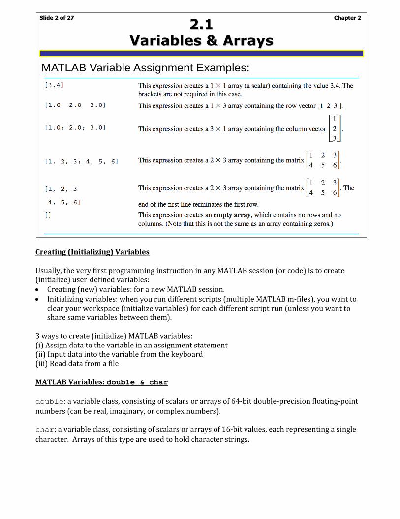
Creating (Initializing) Variables Usually, the very first programming instruction in any MATLAB session (or code) is to create (initialize) user-defined variables: • Creating (new) variables: for a new MATLAB session. • Initializing variables: when you run different scripts (multiple MATLAB m-files), you want to
clear your workspace (initialize variables) for each different script run (unless you want to share same variables between them).
3 ways to create (initialize) MATLAB variables: (i) Assign data to the variable in an assignment statement (ii) Input data into the variable from the keyboard (iii) Read data from a file MATLAB Variables: double & char double: a variable class, consisting of scalars or arrays of 64-bit double-precision floating-point numbers (can be real, imaginary, or complex numbers). char: a variable class, consisting of scalars or arrays of 16-bit values, each representing a single character. Arrays of this type are used to hold character strings.
Chapter 2Slide 2 of 27
2.1 Variables & Arrays
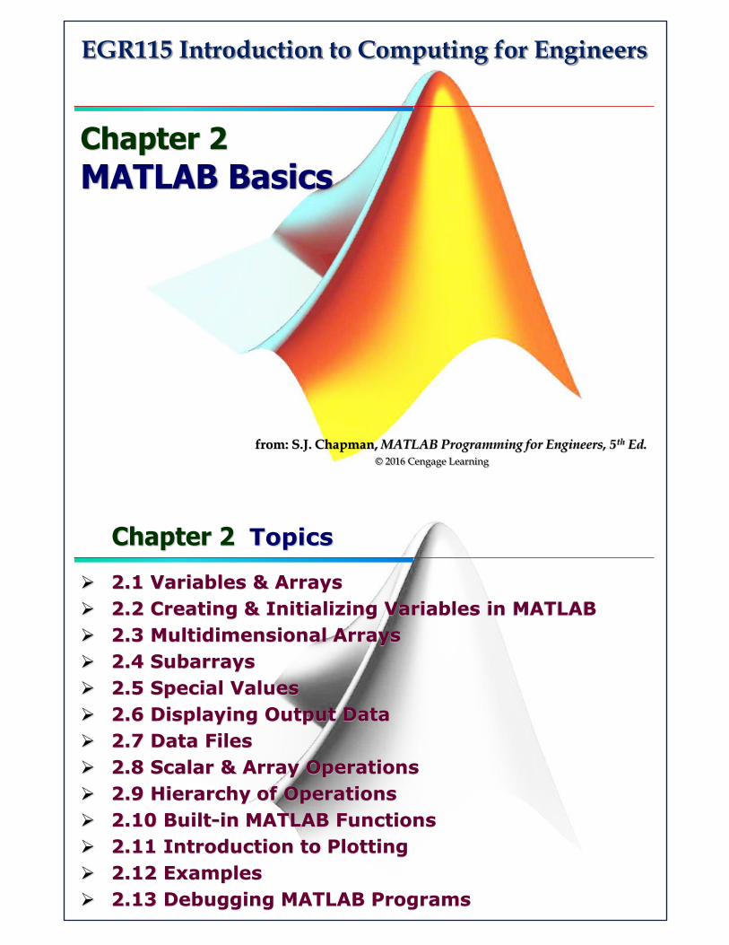
MATLAB Variable Assignment Examples:
(a) Assignment statement
(b) Keyboard inputs
(c) Shortcut expressions
Chapter 2Slide 3 of 27
2.2 Creating & Initializing Variables in MATLAB
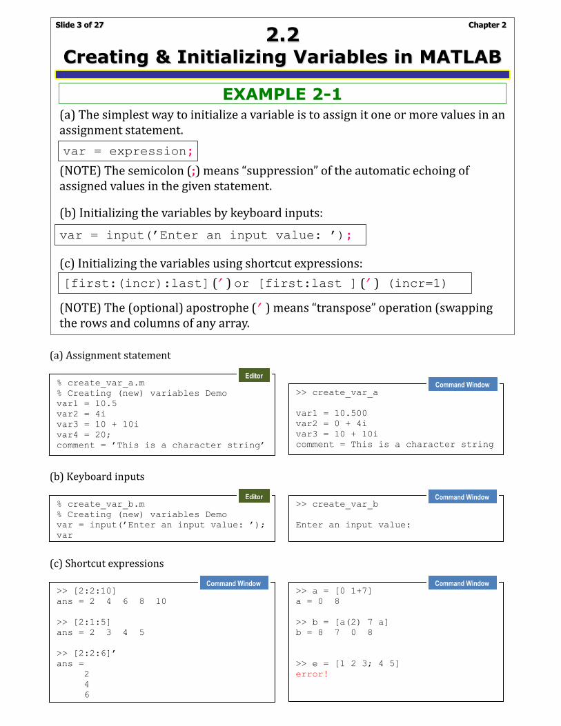
(a) The simplest way to initialize a variable is to assign it one or more values in an assignment statement.
var = expression ;
(NOTE) The semicolon (;) means “suppression” of the automatic echoing of assigned values in the given statement.
EXAMPLE 2-1
(c) Initializing the variables using shortcut expressions:
[first:(incr):last] ( ) or [first:last ] ( ) (incr=1)
(NOTE) The (optional) apostrophe ( ) means “transpose” operation (swapping the rows and columns of any array.
var = input(’Enter an input value: ’) ;
(b) Initializing the variables by keyboard inputs:
% create_var_a.m
% Creating (new) variables Demo
var1 = 10.5
var2 = 4i
var3 = 10 + 10i
var4 = 20;
comment = ’This is a character string’
>> create_var_a
var1 = 10.500
var2 = 0 + 4i
var3 = 10 + 10i
comment = This is a character string
% create_var_b.m
% Creating (new) variables Demo
var = input(’Enter an input value: ’);
var
>> create_var_b
Enter an input value:
>> [2:2:10]
ans = 2 4 6 8 10
>> [2:1:5]
ans = 2 3 4 5
>> [2:2:6]’
ans =
2
4
6
>> a = [0 1+7]
a = 0 8
>> b = [a(2) 7 a]
b = 8 7 0 8
>> e = [1 2 3; 4 5]
error!
Editor
Command Window
Editor Command Window
Command Window Command Window
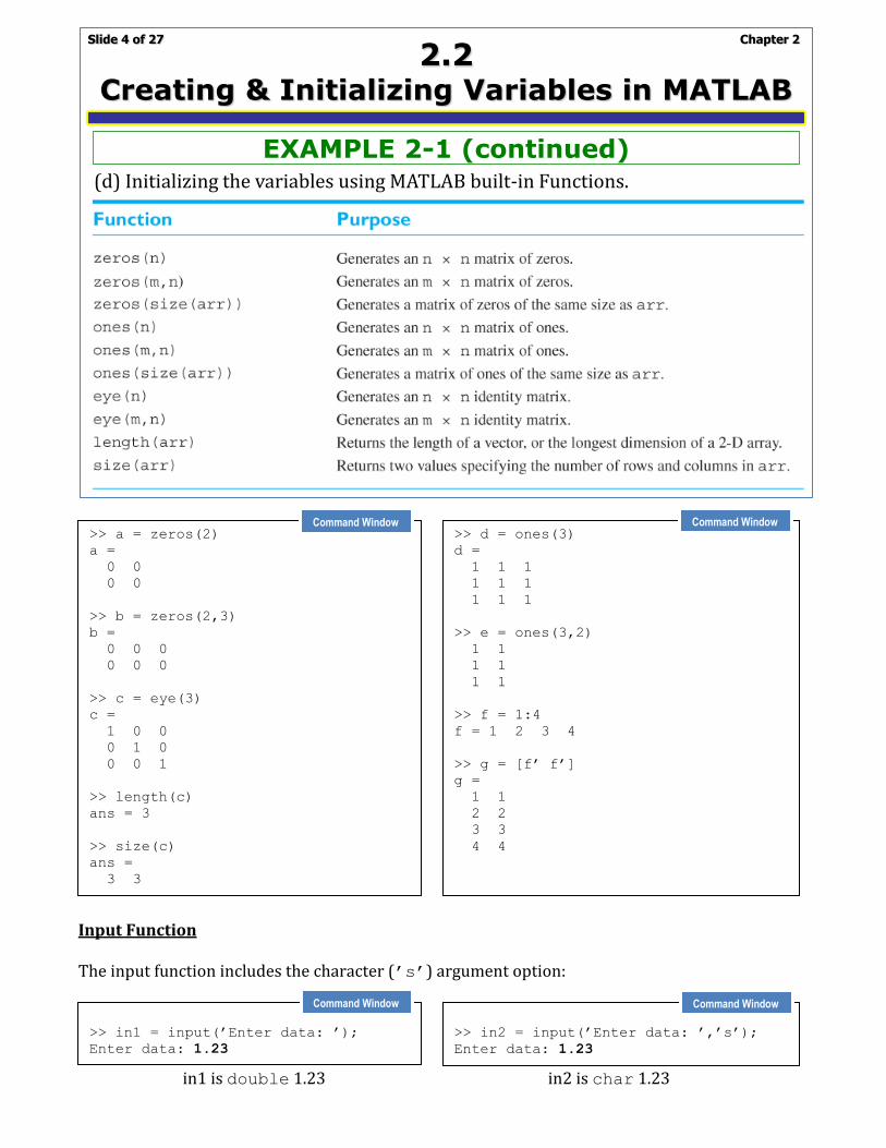
Input Function The input function includes the character (’s’) argument option:
in1 is double 1.23 in2 is char 1.23
Chapter 2Slide 4 of 27
2.2 Creating & Initializing Variables in MATLAB
(d) Initializing the variables using MATLAB built-in Functions.
EXAMPLE 2-1 (continued)
>> a = zeros(2)
a =
0 0
0 0
>> b = zeros(2,3)
b =
0 0 0
0 0 0
>> c = eye(3)
c =
1 0 0
0 1 0
0 0 1
>> length(c)
ans = 3
>> size(c)
ans =
3 3
>> d = ones(3)
d =
1 1 1
1 1 1
1 1 1
>> e = ones(3,2)
1 1
1 1
1 1
>> f = 1:4
f = 1 2 3 4
>> g = [f’ f’]
g =
1 1
2 2
3 3
4 4
>> in1 = input(’Enter data: ’);
Enter data: 1.23
>> in2 = input(’Enter data: ’,’s’);
Enter data: 1.23
Command Window Command Window
Command Window Command Window
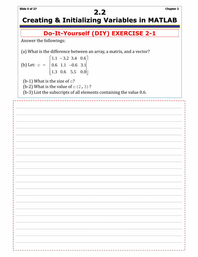
(a) • In MATLAB, an array is a collection of data values organized into rows (m) & columns (n) with
a given single name. The array is the fundamental unit of data in any MATLAB program. • A MATLAB array can be categorized into vector (1-D array) or matrix (2-D array). (b) exercise_2_1b.m
• c(1,4), c(2,1), and c(3,2) are the elements containing the value of 0.6
Chapter 2Slide 5 of 27
2.2 Creating & Initializing Variables in MATLAB
Do-It-Yourself (DIY) EXERCISE 2-1Answer the followings:
(a) What is the difference between an array, a matrix, and a vector?
(b) Let: c =
(b-1) What is the size of c?(b-2) What is the value of c(2,3)?
(b-3) List the subscripts of all elements containing the value 0.6.
1.1 3.2 3.4 0.6
0.6 1.1 0.6 3.1
1.3 0.6 5.5 0.0
− −
% exercise_2_1b.m
%
c = [1.1 -3.2 3.4 0.6;
0.6 1.1 -0.6 3.1;
1.3 0.6 5.5 0.0]
%
b_1 = size(c)
b_2 = c(2,3)
%
c_1_1 = c(1,1)
c_1_2 = c(1,2)
c_1_3 = c(1,3)
c_1_4 = c(1,4)
c_2_1 = c(2,1)
c_2_2 = c(2,2)
c_2_3 = c(2,3)
c_2_4 = c(2,4)
c_3_1 = c(3,1)
c_3_2 = c(3,2)
c_3_3 = c(3,3)
c_3_4 = c(3,4)
>> exercise_2_1b
c =
1.10000 -3.20000 3.40000 0.60000
b_1 =
3 4
b_2 = -0.60000
c_1_1 = 1.1000
c_1_2 = -3.2000
c_1_3 = 3.4000
c_1_4 = 0.60000
c_2_1 = 0.60000
c_2_2 = 1.1000
c_2_3 = -0.60000
c_2_4 = 3.1000)
c_3_1 = 1.3000
c_3_2 = 0.60000
c_3_3 = 5.5000
c_3_4 = 0
Editor Command Window
_________________________________________________________
_________________________________________________________
_________________________________________________________
_________________________________________________________
_________________________________________________________
_________________________________________________________
_________________________________________________________
_________________________________________________________
_________________________________________________________
_________________________________________________________
_________________________________________________________
_________________________________________________________
_________________________________________________________
_________________________________________________________
_________________________________________________________
_________________________________________________________
_________________________________________________________
_________________________________________________________
_________________________________________________________
_________________________________________________________
_________________________________________________________
_________________________________________________________
_________________________________________________________
_________________________________________________________

exercise_2_2_var.m
Chapter 2Slide 6 of 27
2.2 Creating & Initializing Variables in MATLAB
Do-It-Yourself (DIY) EXERCISE 2-2Determine the size of the following arrays, using MATLAB Command Window. Check your answers by entering the arrays into MATLAB and using whos
command (or checking the Workspace Browser).
Note that the later arrays may depend on the definitions of arrays defined earlier in this exercise.
(a) u = [10 20*i 10+20];
(b) v = [-1; 20; 3];
(c) w = [1 0 -9; 2 -2 0; 1 2 3];
(d) x = [u’ v];
(e) y(3,3) = -7;
(f) z = [zeros(4,1) ones(4,1) zeros(1,4)’];
(g) v(4) = x(2,1);
_________________________________________________________
_________________________________________________________
_________________________________________________________
_________________________________________________________
_________________________________________________________
_________________________________________________________
_________________________________________________________
_________________________________________________________
_________________________________________________________
_________________________________________________________
_________________________________________________________
_________________________________________________________
_________________________________________________________
_________________________________________________________
_________________________________________________________
_________________________________________________________
_________________________________________________________
_________________________________________________________
_________________________________________________________
exercise_2_2_var.m
Chapter 2Slide 7 of 27
2.2 Creating & Initializing Variables in MATLAB
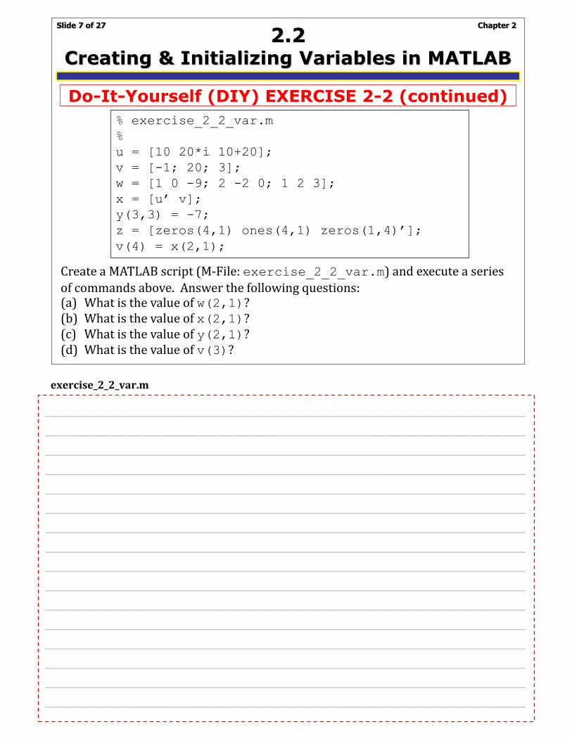
Do-It-Yourself (DIY) EXERCISE 2-2 (continued)
% exercise_2_2_var.m
%
u = [10 20*i 10+20];
v = [-1; 20; 3];
w = [1 0 -9; 2 -2 0; 1 2 3];
x = [u’ v];
y(3,3) = -7;
z = [zeros(4,1) ones(4,1) zeros(1,4)’];
v(4) = x(2,1);
Create a MATLAB script (M-File: exercise_2_2_var.m) and execute a series
of commands above. Answer the following questions:(a) What is the value of w(2,1)? (b) What is the value of x(2,1)? (c) What is the value of y(2,1)? (d) What is the value of v(3)?
% exercise_2_2_var.m
%
u = [10 20*i 10+20];
v = [-1; 20; 3];
w = [1 0 -9; 2 -2 0; 1 2 3];
x = [u’ v];
y(3,3) = -7;
z = [zeros(4,1) ones(4,1)
zeros(1,4)’];
v(4) = x(2,1);
%
w_2_1 = w(2,1)
x_2_1 = x(2,1)
y_2_1 = y(2,1)
v_3 = v(3)
>> exercise_2_2_var
w_2_1 = 2
x_2_1 = 0 – 20i
y_2_1 = 0
v_3 = 3
Editor Command Window _________________________________________________________
_________________________________________________________
_________________________________________________________
_________________________________________________________
_________________________________________________________
_________________________________________________________
_________________________________________________________
_________________________________________________________
_________________________________________________________
_________________________________________________________
_________________________________________________________
_________________________________________________________
_________________________________________________________
_________________________________________________________
_________________________________________________________
_________________________________________________________
_________________________________________________________
_________________________________________________________
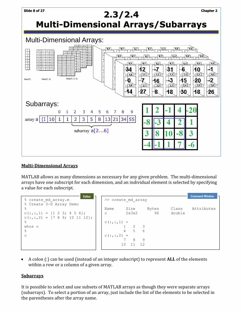
Multi-Dimensional Arrays MATLAB allows as many dimensions as necessary for any given problem. The multi-dimensional arrays have one subscript for each dimension, and an individual element is selected by specifying a value for each subscript.
• A colon (:) can be used (instead of an integer subscript) to represent ALL of the elements
within a row or a column of a given array. Subarrays It is possible to select and use subsets of MATLAB arrays as though they were separate arrays (subarrays). To select a portion of an array, just include the list of the elements to be selected in the parentheses after the array name.
Chapter 2Slide 8 of 27
2.3/2.4 Multi-Dimensional Arrays/Subarrays
Multi-Dimensional Arrays:
Subarrays:
% create_md_array.m
% Create 3-D Array Demo
%
c(:,:,1) = [1 2 3; 4 5 6];
c(:,:,2) = [7 8 9; 10 11 12];
%
whos c
%
c
>> create_md_array
Name Size Bytes Class Attributes
c 2x3x2 96 double
c(:,:,1) =
1 2 3
4 5 6
c(:,:,2) =
7 8 9
10 11 12
Editor Command Window

Subarrays (Example)
• The last command: the elements: arr4(1,1) arr4(1,4) arr4(2,1), and arr4(2,4)
were updated with new values. In order to make this command legal, the array “shape” (numbers of rows & columns) MUST be the same on both sides of the equal sign (else, MATLAB gives an error).
Chapter 2Slide 9 of 27
2.5 Special Values
MATLAB Special Values
% create_subarray.m
% Create Subarray Demo
%
arr1 = [1.1 -2.2 3.3 -4.4 5.5];
%
arr1a = arr1(3)
arr1b = arr1([1 4])
arr1c = arr1(1:2:5)
%
arr2 = [1 2 3; -2 -3 -4; 3 4 5];
%
arr2a = arr2(1,:)
arr2b = arr2(:,1:2:3)
%
arr3 = [1 2 3 4 5 6 7 8];
%
arr3a = arr3(5:end)
arr3b = arr3(end)
%
arr4 = [1 2 3 4; 5 6 7 8; 9 10 11 12];
%
arr4a = arr4(2:end, 2:end)
%
arr4
arr4(1:2,[1 4]) = [20 21; 22 23]
>> create_subarray
arr1a = 3.3000
arr1b =
1.1000 -4.4000
arr1c =
1.1000 3.3000 5.5000
arr2a =
1 2 3
arr2b =
1 3
-2 -4
3 5
arr3a =
5 6 7 8
arr3b = 8
arr4a =
6 7 8
10 11 12
arr4 =
1 2 3 4
5 6 7 8
9 10 11 12
arr4 =
20 2 3 21
22 6 7 23
9 10 11 12
Editor Command Window
Type “clock” & “date” in command window . . .
exercise_2_3_1.m
• (d): c(6) = c(3,2) WHY??? Since MATLAB (in fact) stores data in column major order, one
can (actually) treat a multidimensional array as though it were a 1-D array whose length is equal to the number of elements in the multidimensional array . . . (NOTE) under normal circumstance, you should never use this feature of MATLAB!
Chapter 2Slide 10 of 27
2.5 Special Values
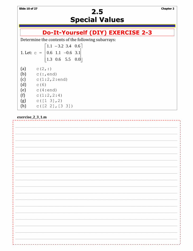
Do-It-Yourself (DIY) EXERCISE 2-3Determine the contents of the following subarrays:
1. Let: c =
(a) c(2,:)
(b) c(:,end)
(c) c(1:2,2:end)
(d) c(6)
(e) c(4:end)
(f) c(1:2,2:4)
(g) c([1 3],2)
(h) c([2 2],[3 3])
1.1 3.2 3.4 0.6
0.6 1.1 0.6 3.1
1.3 0.6 5.5 0.0
− −
% exercise_2_3_1.m
%
c = [1.1 -3.2 3.4 0.6;
0.6 1.1 -0.6 3.1;
1.3 0.6 5.5 0.0];
%
c_a = c(2,:)
%
c_b = c(:,end)
%
c_c = c(1:2,2:end)
%
c_d = c(6)
%
c_e = c(4:end)
%
c_f = c(1:2,2:4)
%
c_g = c([1 3],2)
%
c_h = c([2 2],[3 3])
>> exercise_2_3_1
c_a =
0.60000 1.10000 -0.60000 3.10000
c_b =
0.60000
3.10000
0.00000
c_c =
-3.20000 3.40000 0.60000
1.10000 -0.60000 3.10000
c_d = 0.60000
c_e =
-3.20000 1.10000 0.60000 3.40000 -0.60000
5.50000 0.60000 3.10000 0.00000
c_f =
-3.20000 3.40000 0.60000
1.10000 -0.60000 3.10000
c_g =
-3.20000
0.60000
c_h =
-0.60000 -0.60000
-0.60000 -0.60000
Editor Command Window _________________________________________________________
_________________________________________________________
_________________________________________________________
_________________________________________________________
_________________________________________________________
_________________________________________________________
_________________________________________________________
_________________________________________________________
_________________________________________________________
_________________________________________________________
_________________________________________________________
_________________________________________________________
_________________________________________________________
_________________________________________________________
_________________________________________________________
_________________________________________________________
_________________________________________________________
_________________________________________________________
_________________________________________________________
_________________________________________________________
exercise_2_3_2.m / exercise_2_3_3.m
Chapter 2Slide 11 of 27
2.5 Special Values
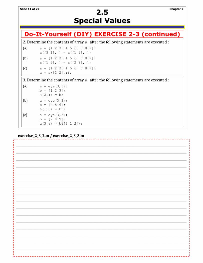
Do-It-Yourself (DIY) EXERCISE 2-3 (continued)
2. Determine the contents of array a after the following statements are executed :
(a) a = [1 2 3; 4 5 6; 7 8 9];
a([3 1],:) = a([1 3],:);
(b) a = [1 2 3; 4 5 6; 7 8 9];
a([1 3],:) = a([2 2],:);
(c) a = [1 2 3; 4 5 6; 7 8 9];
a = a([2 2],:);
3. Determine the contents of array a after the following statements are executed :
(a) a = eye(3,3);
b = [1 2 3];
a(2,:) = b;
(b) a = eye(3,3);
b = [4 5 6];
a(:,3) = b’;
(c) a = eye(3,3);
b = [7 8 9];
a(3,:) = b([3 1 2]);
% exercise_2_3_2.m
%
a = [1 2 3; 4 5 6; 7 8 9];
a([3 1],:) = a([1 3],:);
a_a = a
%
a = [1 2 3; 4 5 6; 7 8 9];
a([1 3],:) = a([2 2],:);
a_b = a
%
a = [1 2 3; 4 5 6; 7 8 9];
a_c = a([2 2],:)
>> exercise_2_3_2
a_a =
7 8 9
4 5 6
1 2 3
a_b =
4 5 6
4 5 6
4 5 6
a_b =
4 5 6
4 5 6
% exercise_2_3_3.m
%
a = eye(3,3);
b = [1 2 3];
a(2,:) = b;
a_a = a
%
a = eye(3,3);
b = [4 5 6];
a(:,3) = b';
a_b = a
%
a = eye(3,3);
b = [7 8 9];
a(3,:) = b([3 1 2]);
a_c = a
>> exercise_2_3_3
a_a =
1 0 0
1 2 3
0 0 1
a_b =
1 0 4
0 1 5
0 0 6
a_c =
1 0 0
0 1 0
9 7 8
Editor Command Window
Editor Command Window
_________________________________________________________
_________________________________________________________
_________________________________________________________
_________________________________________________________
_________________________________________________________
_________________________________________________________
_________________________________________________________
_________________________________________________________
_________________________________________________________
_________________________________________________________
_________________________________________________________
_________________________________________________________
_________________________________________________________
_________________________________________________________
_________________________________________________________
_________________________________________________________
_________________________________________________________
_________________________________________________________
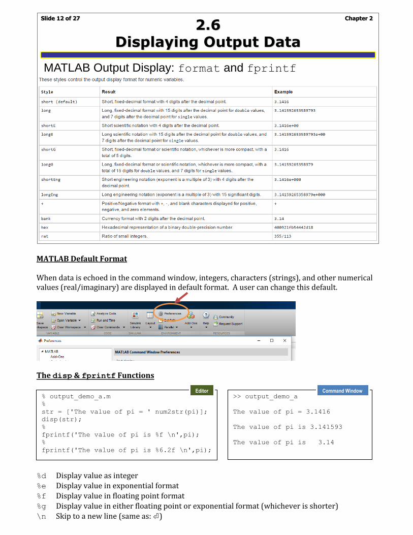
MATLAB Default Format When data is echoed in the command window, integers, characters (strings), and other numerical values (real/imaginary) are displayed in default format. A user can change this default.
The disp & fprintf Functions
%d Display value as integer %e Display value in exponential format %f Display value in floating point format
%g Display value in either floating point or exponential format (whichever is shorter) \n Skip to a new line (same as: ⏎)
Chapter 2Slide 12 of 27
2.6 Displaying Output Data
MATLAB Output Display: format and fprintf
% output_demo_a.m
%
str = ['The value of pi = ' num2str(pi)];
disp(str);
%
fprintf('The value of pi is %f \n',pi);
%
fprintf('The value of pi is %6.2f \n',pi);
>> output_demo_a
The value of pi = 3.1416
The value of pi is 3.141593
The value of pi is 3.14
Editor Command Window
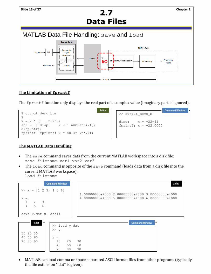
The Limitation of fprintf The fprintf function only displays the real part of a complex value (imaginary part is ignored).
The MATLAB Data Handling • The save command saves data from the current MATLAB workspace into a disk file:
save filename var1 var2 var3
• The load command is opposite of the save command (loads data from a disk file into the current MATLAB workspace): load filename
• MATLAB can load comma or space separated ASCII format files from other programs (typically
the file extension “.dat” is given).
Chapter 2Slide 13 of 27
2.7 Data Files
MATLAB Data File Handling: save and load
I/O
% output_demo_b.m
%
x = 2 * (1 - 2i)^3;
str = ['disp: x = ' num2str(x)];
disp(str);
fprintf('fprintf: x = %8.4f \n',x);
>> output_demo_b
disp: x = -22+4i
fprintf: x = -22.0000
>> x = [1 2 3; 4 5 6]
x =
1 2 3
4 5 6
save x.dat x -ascii
1.00000000e+000 2.00000000e+000 3.00000000e+000
4.00000000e+000 5.00000000e+000 6.00000000e+000
10 20 30
40 50 60
70 80 90
>> load y.dat
>> y
y =
10 20 30
40 50 60
70 80 90
Editor Command Window
Command Window x.dat
y.dat Command Window
exercise_2_4_2.m / exercise_2_4_3.m 1. “format long e” will display all real values in exponential format with 15 significant digits. 2. exercise_2_4_2.m
3. exercise_2_4_3.m
Chapter 2Slide 14 of 27
2.7 Data Files
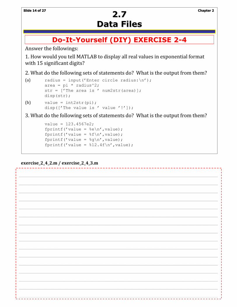
Do-It-Yourself (DIY) EXERCISE 2-4Answer the followings:
1. How would you tell MATLAB to display all real values in exponential format with 15 significant digits?
2. What do the following sets of statements do? What is the output from them?
(a) radius = input(’Enter circle radius:\n’);
area = pi * radius^2;
str = [’The area is ’ num2str(area)];
disp(str);
(b) value = int2str(pi);
disp([’The value is ’ value ’!’]);
3. What do the following sets of statements do? What is the output from them?
value = 123.4567e2;
fprintf(’value = %e\n’,value);
fprintf(’value = %f\n’,value);
fprintf(’value = %g\n’,value);
fprintf(’value = %12.4f\n’,value);
% exercise_2_4_2.m
% (a)
radius = input('Enter circle radius:\n');
area = pi*radius^2;
str = ['The area is ' num2str(area)];
disp(str);
disp(' ');
disp('Hit Enter to continue . . .');
disp(' ');
pause
% (b)
value = int2str(pi);
disp(['The value is ' value '!']);
>> exercise_2_4_2
Enter circle radius:
25
The area is 1963.4954
Hit Enter to continue . . .
The value is 3!
% exercise_2_4_3.m
value = 123.4567e2;
fprintf('value = %e\n',value);
fprintf('value = %f\n',value);
fprintf('value = %g\n',value);
fprintf('value = %12.4f\n',value);
>> exercise_2_4_3
value = 1.234567e+04
value = 12345.670000
value = 12345.7
value = 12345.6700
Editor Command Window
Editor Command Window
_________________________________________________________
_________________________________________________________
_________________________________________________________
_________________________________________________________
_________________________________________________________
_________________________________________________________
_________________________________________________________
_________________________________________________________
_________________________________________________________
_________________________________________________________
_________________________________________________________
_________________________________________________________
_________________________________________________________
_________________________________________________________
_________________________________________________________
_________________________________________________________
_________________________________________________________
_________________________________________________________

MATLAB Calculations (Operations) MATLAB performs calculations (like a calculator) with an assignment statement: variable_name = expression;
(this is NOT math: store the value of expression into the location variable_name) MATLAB Arithmetic Operators (for Scalars) Addition (a + b): a + b
Subtraction (a − b): a - b
Multiplication (a b): a * b
Division (a b): a / b
Exponentiation (ab): a ^ b
MATLAB Array & Matrix Operators (for Vectors & Matrices) • Array operations: operations performed between arrays on an element-by-element basis. • Matrix operations: follow the normal rules of linear algebra (if you don’t know what it means . . . see this: https://www.mathsisfun.com/algebra/matrix-multiplying.html)
(NOTE: these are fundamentally very different mathematical operations: be very careful) https://www.mathworks.com/help/matlab/matlab_prog/array-vs-matrix-operations.html
Chapter 2Slide 15 of 27
2.8 Scalar & Array Operations
MATLAB Array & Matrix Operations
>> example_2_2
ans_a =
0 2
2 2
ans_b =
-1 0
0 1
ans_c =
-1 2
-2 5
ans_d =
3
8
ans_f =
6 5
7 6
ans_g =
5 0
10 5
ans_h =
5 0
10 5
example_2_2.m
Chapter 2Slide 16 of 27
2.8 Scalar & Array Operations
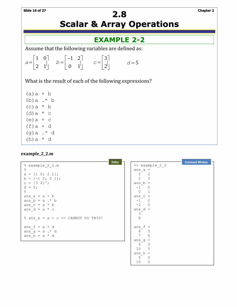
Assume that the following variables are defined as:
What is the result of each of the following expressions?
(a)a + b
(b)a .* b
(c)a * b
(d)a * c
(e)a + c
(f)a + d
(g)a .* d
(h)a * d
EXAMPLE 2-2
1 0
2 1
=
a
1 2
0 1
− =
b
3
2
=
c 5=d
% example_2_2.m
%
a = [1 0; 2 1];
b = [-1 2; 0 1];
c = [3 2]';
d = 5;
%
ans_a = a + b
ans_b = a .* b
ans_c = a * b
ans_d = a * c
% ans_e = a + c <= CANNOT DO THIS!
ans_f = a + d
ans_g = a .* d
ans_h = a * d
Editor Command Window
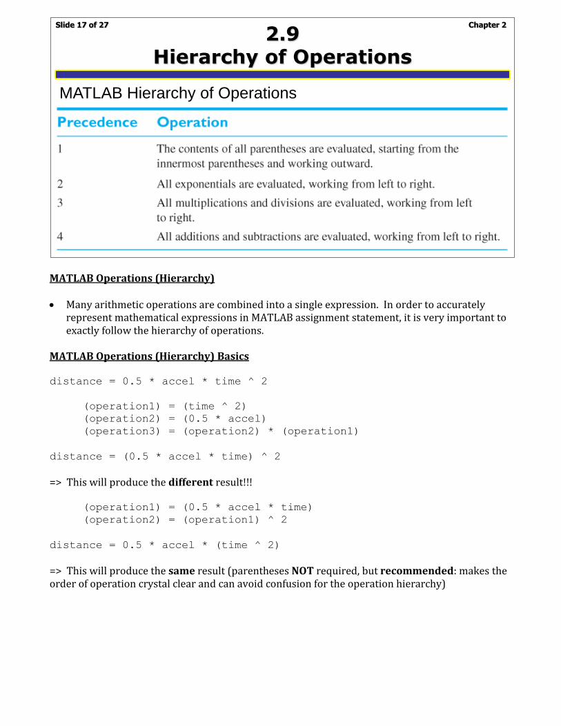
MATLAB Operations (Hierarchy) • Many arithmetic operations are combined into a single expression. In order to accurately
represent mathematical expressions in MATLAB assignment statement, it is very important to exactly follow the hierarchy of operations.
MATLAB Operations (Hierarchy) Basics distance = 0.5 * accel * time ^ 2
(operation1) = (time ^ 2)
(operation2) = (0.5 * accel)
(operation3) = (operation2) * (operation1) distance = (0.5 * accel * time) ^ 2
=> This will produce the different result!!! (operation1) = (0.5 * accel * time)
(operation2) = (operation1) ^ 2
distance = 0.5 * accel * (time ^ 2)
=> This will produce the same result (parentheses NOT required, but recommended: makes the order of operation crystal clear and can avoid confusion for the operation hierarchy)
Chapter 2Slide 17 of 27
2.9 Hierarchy of Operations
MATLAB Hierarchy of Operations

MATLAB Operations (Hierarchy): Some Important Professional Practices • It is extremely important that every expression in a program be made as clear as possible. • Ask yourself a series of questions: “Can I easily understand this expression if I come back to it
in 6 month?” “Can another programmer look at my code and instantly understand what my instructions are?”
• If you are not sure, use extra parentheses in the expression to make it sure. • Alternatively, separate your expression into a few parts (avoid using extremely long
mathematical expression in a single line). (a) output = a*b+c*d = 3*2+5*3
= (3 * 2) + (5 * 3) = 6 + (5 * 3) = 6 + 15 = 21
(b) output = a*(b+c)*d = 3*(2+5)*3
= 3 * (2 + 5) * 3 = 3 * 7 * 3 = 21 * 3 = 63
(c) output = (a*b)+(c*d) = (3*2)+(5*3)
= (3 * 2) + (5 * 3) = 6 + (5 * 3) = 6 + 15 = 21
(d) output = a^b^d = 3^2^3
= (3 ^ 2) ^ 3 = 9 ^ 3 = 729
(e) output = a^(b^d) = 3^(2^3)
= 3 ^ (2 ^ 3) = 3 ^ 8 = 6561
Chapter 2Slide 18 of 27
2.9 Hierarchy of Operations
Variables a, b, c, and d have been initialized to the following vales:a = 3; b = 2; c = 5; d = 3;
Evaluate the following MATLAB assignment statements, showing the details of hierarchy of operations.
(a)output = a*b+c*d;
(b)output = a*(b+c)*d;
(c)output = (a*b)+(c*d);
(d)output = a^b^d;
(e)output = a^(b^d);
EXAMPLE 2-3
exercise_2_5.m
Chapter 2Slide 19 of 27
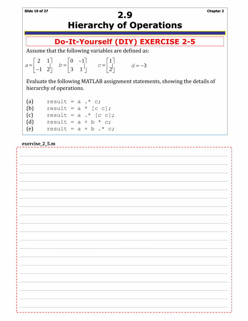
2.9 Hierarchy of Operations
Do-It-Yourself (DIY) EXERCISE 2-5Assume that the following variables are defined as:
Evaluate the following MATLAB assignment statements, showing the details of hierarchy of operations.
(a) result = a .* c;
(b) result = a * [c c];
(c) result = a .* [c c];
(d) result = a + b * c;
(e) result = a + b .* c;
2 1
1 2
= −
a0 1
3 1
− =
b
1
2
=
c 3= −d
% exercise_2_5.m
%
a = [2 1; -1 2];
b = [0 -1; 3 1];
c = [1 2]';
d = -3;
% result_a = a .* c <= CANNOT DO THIS!
result_b = a * [c c]
result_c = a .* [c c]
% result_d = a + b * c <= CANNOT DO THIS!
% result_e = a + b .* c <= CANNOT DO THIS!
>> exercise_2_5
result_b =
4 4
3 3
result_c =
2 1
-2 4
Editor Command Window _________________________________________________________
_________________________________________________________
_________________________________________________________
_________________________________________________________
_________________________________________________________
_________________________________________________________
_________________________________________________________
_________________________________________________________
_________________________________________________________
_________________________________________________________
_________________________________________________________
_________________________________________________________
_________________________________________________________
_________________________________________________________
_________________________________________________________
_________________________________________________________
_________________________________________________________
_________________________________________________________
_________________________________________________________
_________________________________________________________
_________________________________________________________

exercise_2_6.m
Chapter 2Slide 20 of 27
2.9 Hierarchy of Operations
Do-It-Yourself (DIY) EXERCISE 2-6Solve for x in the equation Ax = B, where:
1 2 1
2 3 2
1 0 1
= −
A
1
1
0
=
B
11 1 12 2 13 3 1
21 1 22 2 23 3 2
31 1 32 2 33 3 3
a x a x a x b
a x a x a x b
a x a x a x b
+ + =
+ + =
+ + =
Understand that you are solving a set of simultaneous linear equations:
This can be solved by a multiplication of Matrix Inverse of A and B, as:
Ax B= 11 12 13
21 22 23
31 32 33
a a a
a a a
a a a
=
A1
2
3
b
b
b
=
B1
2
3
x
x x
x
=
1x A B−=
In MATLAB, the Matrix Left Division will do the job . . .
A \ B <= which is defined as: inv(A) * B
% exercise_2_6.m
% Simultaneous Linear Equations Solver
%
A = [1 2 1; 2 3 2; -1 0 1];
B = [1 1 0]';
%
x = A \ B;
x
%
x = inv(A)*B
x
%
x1 = x(1)
x2 = x(2)
x3 = x(3)
>> exercise_2_6
x =
-0.5000
1.0000
-0.5000
x1 = -0.5000
x2 = 1.0000
x3 = -0.5000
Editor Command Window _________________________________________________________
_________________________________________________________
_________________________________________________________
_________________________________________________________
_________________________________________________________
_________________________________________________________
_________________________________________________________
_________________________________________________________
_________________________________________________________
_________________________________________________________
_________________________________________________________
_________________________________________________________
_________________________________________________________
_________________________________________________________
_________________________________________________________
_________________________________________________________
_________________________________________________________
_________________________________________________________
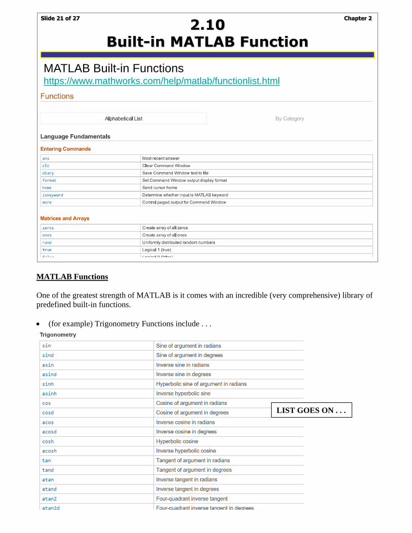
MATLAB Functions
One of the greatest strength of MATLAB is it comes with an incredible (very comprehensive) library of
predefined built-in functions.
• (for example) Trigonometry Functions include . . .
Chapter 2Slide 21 of 27
2.10 Built-in MATLAB Function
MATLAB Built-in Functionshttps://www.mathworks.com/help/matlab/functionlist.html
LIST GOES ON . . .
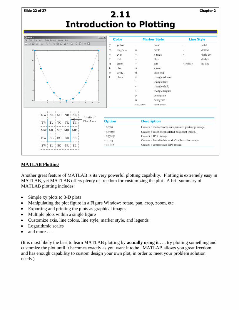
MATLAB Plotting
Another great feature of MATLAB is its very powerful plotting capability. Plotting is extremely easy in
MATLAB, yet MATLAB offers plenty of freedom for customizing the plot. A brif summary of
MATLAB plotting includes:
• Simple xy plots to 3-D plots
• Manipulating the plot figure in a Figure Window: rotate, pan, crop, zoom, etc.
• Exporting and printing the plots as graphical images
• Multiple plots within a single figure
• Customize axis, line colors, line style, marker style, and legends
• Logarithmic scales
• and more . . .
(It is most likely the best to learn MATLAB plotting by actually using it . . . try plotting something and
customize the plot until it becomes exactly as you want it to be. MATLAB allows you great freedom
and has enough capability to custom design your own plot, in order to meet your problem solution
needs.)
Chapter 2Slide 22 of 27
2.11 Introduction to Plotting
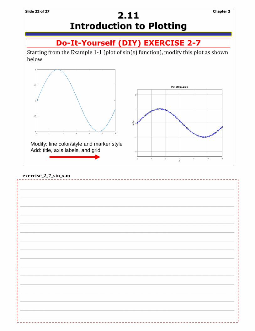
exercise_2_7_sin_x.m
Chapter 2Slide 23 of 27
2.11 Introduction to Plotting
Do-It-Yourself (DIY) EXERCISE 2-7Starting from the Example 1-1 (plot of sin(x) function), modify this plot as shown below:
Modify: line color/style and marker style
Add: title, axis labels, and grid
% exercise_2_7_sin_x.m
%
% Based on: example_1_1_sin_x.m
%
clc
close all
clear all
x = 0:0.1:6;
y = sin(x);
plot(x,y,'k-',x,y,'bo');
%
title('Plot of f(x)=sin(x)');
xlabel('x');
ylabel('sin(x)');
grid on
axis equal
Editor _________________________________________________________
_________________________________________________________
_________________________________________________________
_________________________________________________________
_________________________________________________________
_________________________________________________________
_________________________________________________________
_________________________________________________________
_________________________________________________________
_________________________________________________________
_________________________________________________________
_________________________________________________________
_________________________________________________________
_________________________________________________________
_________________________________________________________
_________________________________________________________
_________________________________________________________
_________________________________________________________
exercise_2_8_cos_x.m
Chapter 2Slide 24 of 27
2.11 Introduction to Plotting
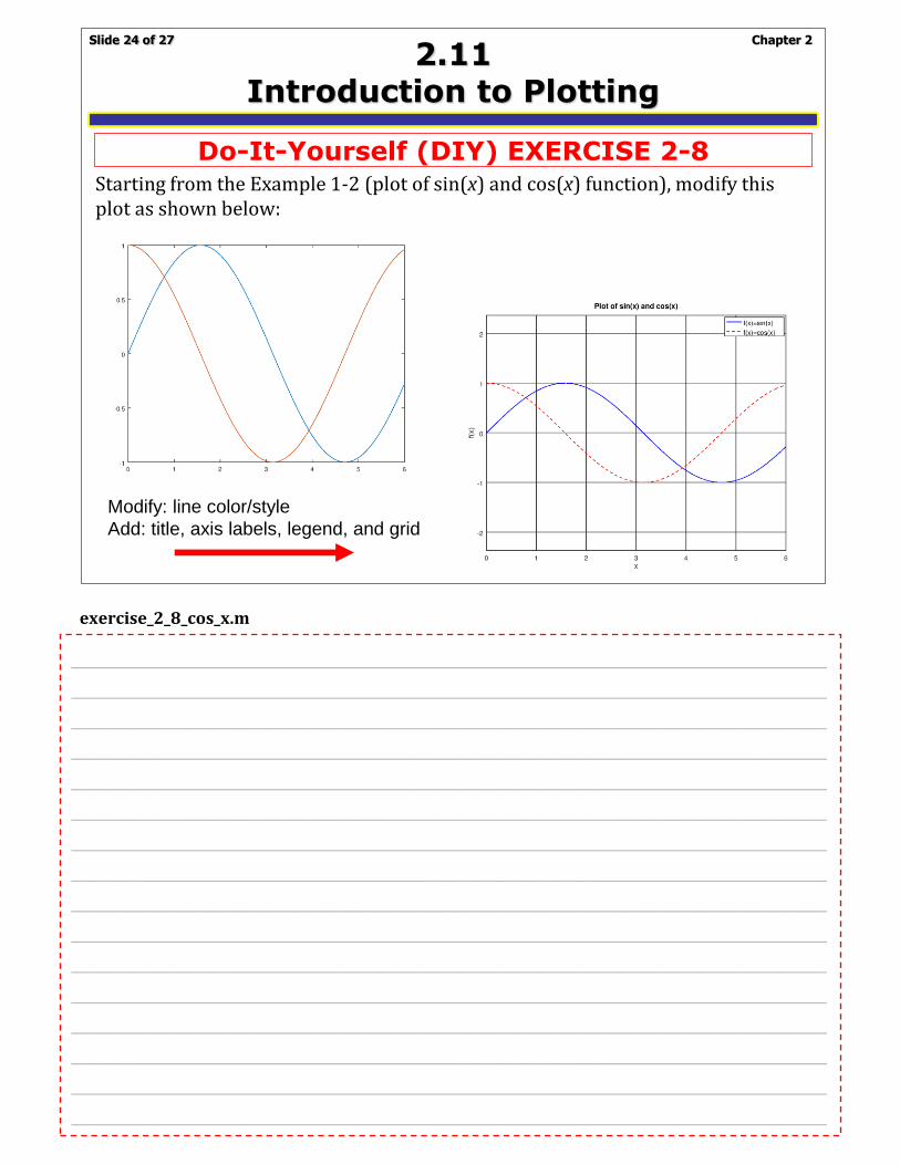
Do-It-Yourself (DIY) EXERCISE 2-8Starting from the Example 1-2 (plot of sin(x) and cos(x) function), modify this plot as shown below:
Modify: line color/style
Add: title, axis labels, legend, and grid
% exercise_2_8_cos_x.m
%
% Based on: example_1_2_cos_x.m
%
clc
clear all
close all
x = 0:0.1:6;
y1 = sin(x);
y2 = cos(x);
plot(x,y1,'b-',x,y2,'r--');
%
title('Plot of sin(x) and cos(x)');
xlabel('x');
ylabel('f(x)');
legend ('f(x)=sin(x)','f(x)=cos(x)')
grid on
axis equal
Editor _________________________________________________________
_________________________________________________________
_________________________________________________________
_________________________________________________________
_________________________________________________________
_________________________________________________________
_________________________________________________________
_________________________________________________________
_________________________________________________________
_________________________________________________________
_________________________________________________________
_________________________________________________________
_________________________________________________________
_________________________________________________________
_________________________________________________________
_________________________________________________________
_________________________________________________________
_________________________________________________________

example_2_4_temp_conversion.m
Chapter 2Slide 25 of 27
2.12 Examples
EXAMPLE 2-4Design a MATLAB program that reads an input temperature in degrees Fahrenheit, converts it to an absolute temperature in kelvin, and writes out the result. The relationship between temperature in degrees Fahrenheit (F) and temperature in kelvins (K) is:
1. Prompt the user to enter an input temperature in F.2. Read the input temperature.3. Calculate the temperature in kelvin.4. Write the result and stop.
( ) ( )5
K F 32.0 273.159
T T
= − +
% Script file: temp_conversion.m
%
% Purpose:
% To convert an input temperature from degrees Fahrenheit to
% an output temperature in kelvin.
%
% Record of revisions:
% Date Programmer Description of change
% ==== ========== =====================
% 01/03/14 S. J. Chapman Original code
%
% Define variables:
% temp_f -- Temperature in degrees Fahrenheit
% temp_k -- Temperature in kelvin
% Prompt the user for the input temperature.
temp_f = input('Enter the temperature in degrees Fahrenheit: ');
% Convert to kelvin.
temp_k = (5/9) * (temp_f - 32) + 273.15;
% Write out the result.
fprintf('%6.2f degrees Fahrenheit = %6.2f kelvin.\n', ...
temp_f,temp_k);
Editor

example_2_5_calc_power.m
Chapter 2Slide 26 of 27
2.12 Examples
EXAMPLE 2-5A voltage source V = 120 V with an internal resistance RS of 50 W is applied to a load of resistance RL. Find the value of load resistance RL that will result in the maximum possible power being supplied by the source to the load. How much power will be supplied in this case? Also, plot the power supplied to the load as a function of the load resistance RL. In this exercise, we need to vary the load resistance RL and compute the power supplied to the load at each value of RL. The power supplied to the load resistance is given by:where I is the current supplied to the load. The current supplied to the load can be calculated by Ohm’s Law:
1. Create an array of possible values for the load resistance.2. Calculate the current for each value of RL.3. Calculate the power supplied to the load.4. Plot the power supplied to the load.
2
L LP I R=
TOT S L
V VI
R R R= =
+
% Script file: calc_power.m
%
% Define variables:
% amps -- Current flow to load (amps)
% pl -- Power supplied to load (watts)
% rl -- Resistance of the load (ohms)
% rs -- Internal resistance of the power source (ohms)
% volts -- Voltage of the power source (volts)
% Set the values of source voltage and internal resistance
volts = 120;
rs = 50;
% Create an array of load resistances
rl = 1:1:100;
% Calculate the current flow for each resistance
amps = volts ./ ( rs + rl );
% Calculate the power supplied to the load
pl = (amps .^ 2) .* rl;
% Plot the power versus load resistance
plot(rl,pl);
title('Plot of power versus load resistance');
xlabel('Load resistance (ohms)');
ylabel('Power (watts)');
grid on;
Editor

Debug a MATLAB Program
MATLAB Errors
3 Types of erros in MATLAB:
(i) Syntax error: errors in the MATLAB statement itself (spelling, punctuation, format, etc.)
(ii) Run-time error: errors when an illegal mathematical operation is attempted during the program
execution (i.e., attempting to divide by zero, producing the infinity). The program returns inf or Nan,
which is then used for further calculations.
(iii) Logical error: errors when the program compiles and runs successfully but produces wrong answer
(the toughest one to discover . . . MATLAB cannot detect this type of error: the program appears to run
OK, but produces wrong results). You must spend some time, trying to debug your code.
The MATLAB Symbolic Debugger
MATLAB offers a powerful tool for debugging, embedded into the MATLAB editor. The MATLAB
symbolic editor allows you to:
• walk through the code execution one statement at a time and to examine the values of any variables
at each step along the way.
• see all of the intermediate results without having to insert a lot of output statements into your code.
Chapter 2Slide 27 of 27
2.13 Debugging MATLAB Programs
Debug a MATLAB Programhttps://www.mathworks.com/help/matlab/matlab_prog/debugging-process-and-features.html